Zero dynamics of SISO quasi-polynomial systems

ZERO DYNAMICS OF SISO

QUASI-POLYNOMIAL SYSTEMS

Tamas Schne, Katalin Hangos

Technical Report SCL-005/2004

Contents

1 Introduction 3

2 Basic notions 4

3 Zero dynamics of LILO QP systems 6

3.1 The r = 1 case . . . . . . . . . . . . . . . . . . . . . . . . . . . . . . . . . . . . . . . . 63.2 The r > 1 case . . . . . . . . . . . . . . . . . . . . . . . . . . . . . . . . . . . . . . . . 73.3 Stability analysis of LILO QP systems . . . . . . . . . . . . . . . . . . . . . . . . . . . 83.4 A simple example . . . . . . . . . . . . . . . . . . . . . . . . . . . . . . . . . . . . . . . 9

4 Case study: heat exchanger cells 11

4.1 The r = 1 case . . . . . . . . . . . . . . . . . . . . . . . . . . . . . . . . . . . . . . . . 134.2 The r > 1 case . . . . . . . . . . . . . . . . . . . . . . . . . . . . . . . . . . . . . . . . 14

5 Conclusions 16

2

Chapter 1

Introduction

Control of nonlinear systems presents a number of challenging nontrivial problems. Appropriate input-output controller structure design for multiple input-multiple output (MIMO) systems is one amongthem, that may be done using zero dynamics.

Most often, a complex nonlinear system description can cause difficulties in investigating basicsystem properties such as controllability, observability or stability. For the latter, a well-known andfrequently used method, the linearization of the system in a neighborhood of an equilibrium point isusually improper. In most cases, even if the system is locally stable the stability region is so narrowthat linear methods cannot be efficiently used for controller design.

Better results can be achieved using quadratic or other simple Lyapunov function candidates forstability region estimation. However, this method has a serious disadvantage: in spite of the existenceof the Lyapunov function, the calculation itself is not trivial.

During the decades different special nonlinear system description forms were published to makeeasier the solution of this problem, such as quasi-polynomial (QP) [6] or Hamiltonian [5] forms. Forthese system classes there are methods to compute Lyapunov function candidates, which are quadratic,by using linear matrix inequalities (LMIs) [7] or bilinear matrix inequalities (BMIs).

For efficient controller design not only the stability of a desired equilibrium should be investigatedbut the stability of the zero dynamics around this point itself. Analysis of the zero dynamics has a keyrole in controller structure selection. When the value of one state variable is selected as an output (aspecial partial state feedback), then the system can be forced to have constant valued output by usinga stable output feedback. If the system has stable zero dynamics then not only that state variablewill remain at its equilibrium value but all other state variables will converge asymptotically to theirequilibrium values in case of a disturbance. However, e.g. in process systems, unstable zero dynamicscan make the remaining state variables of the system go far from the desired values and reach an otherequilibrium point. Form this follows that an appropriate input-output pair which possesses stable zerodynamics can be used for efficient controller structure selection.

3

Chapter 2

Basic notions

Every process system and most nonlinear systems can be written in a so-called input-affine form:

x = f(x) +∑m

i=1 gi(x)ui (state equation)yj = hj(x) j = 1, . . . , p (output equation)

(2.1)

where ui, i = 1, . . . , m denotes the control input, and f , gi and h are smooth nonlinear functions.The m = p = 1 case is called single input-single output (SISO) system. An input-output pair ofinput-affine systems can be characterized by its relative degree. This value is defined at an equilibriumpoint x0, and shows the number of times that the output should be differentiated so that the inputappeared in its derivative.

The exact definition is the following: given a SISO nonlinear system in input-affine form

x = f(x) + g(x)uy = h(x)

(2.2)

with an x0 equilibrium point. Let U be a neighborhood of x0. The system above has relative degreer if

1. LgLkfh(x) = 0 ∀x ∈ U , k < r − 1, and

2. LgLr−1f h(x0) 6= 0

The latter condition is not necessarily fulfilled so the relative degree is not always defined. If r isless than the number of state variables n then the zero dynamics describes the dynamical behavior ofthe system when its output is forced to be identically zero (generally: constant) by a suitable staticnonlinear feedback [3]. The dimension of this dynamics equals to the difference between the numberof state variables and the value of the relative degree.

Every lumped process system can be written in quasi polynomial (QP) form [6]:

xi = xi(λi +m

∑

j=1

Aij

n∏

k=1

xBjk

k ) (2.3)

i = 1, . . . , n m ≥ n, xi > 0

where the constant vector λ ∈ Rn and the real valued constant matrices A ∈ R

n×m and B ∈ Rm×n

are the system parameters. The number m is related to the number of quasi monomials defined by

the terms z =∏n

k=1 xBjk

k . Choosing these monomials as state variables results in the Lotka–Volterraform [2]:

zi = zi(λLVi +

m∑

j=1

Mijzj) (2.4)

4

i = 1, . . . , m

where λLV = Bλ ∈ Rm and M = BA ∈ R

m×m. The importance of these representations is the easierstability analysis of nonlinear systems. However, its is important to note that if the number of quasimonomials is greater than the number of state variables then the matrix M is singular. Singularitycauses the appearance of zero eigenvalues with their number equal to m−n. These eigenvalues shouldnot be taken into account, but only the remaining ones can be used for local stability analysis.

A technical tool for stability analysis is the usage of linear matrix inequalities (LMIs):

F (z) = F0 +m

∑

i=1

ziFi ≥ 0 (2.5)

where z ∈ Rm is the variable and Fi ∈ R

n×n, i = 0, . . . , m are given symmetric matrices. Theinequality symbol represents the positive semi-definiteness of F (z).

5

Chapter 3

Zero dynamics of LILO QP systems

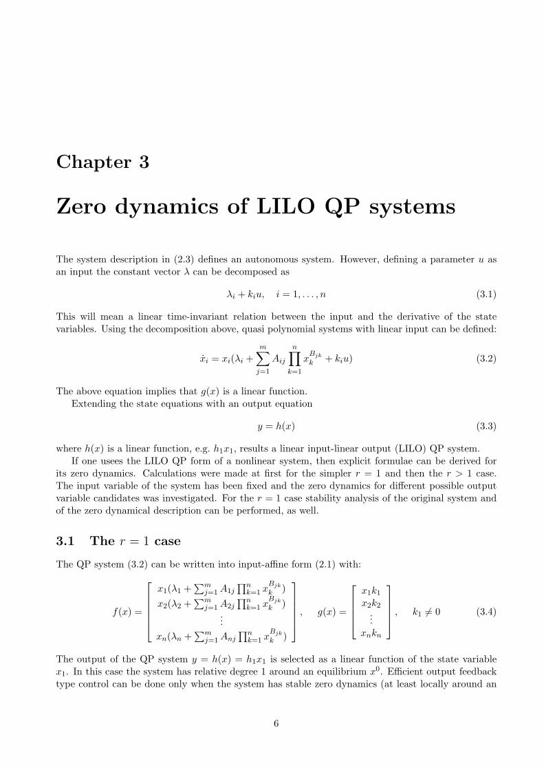
The system description in (2.3) defines an autonomous system. However, defining a parameter u asan input the constant vector λ can be decomposed as

λi + kiu, i = 1, . . . , n (3.1)

This will mean a linear time-invariant relation between the input and the derivative of the statevariables. Using the decomposition above, quasi polynomial systems with linear input can be defined:

xi = xi(λi +

m∑

j=1

Aij

n∏

k=1

xBjk

k + kiu) (3.2)

The above equation implies that g(x) is a linear function.Extending the state equations with an output equation

y = h(x) (3.3)

where h(x) is a linear function, e.g. h1x1, results a linear input-linear output (LILO) QP system.If one usees the LILO QP form of a nonlinear system, then explicit formulae can be derived for

its zero dynamics. Calculations were made at first for the simpler r = 1 and then the r > 1 case.The input variable of the system has been fixed and the zero dynamics for different possible outputvariable candidates was investigated. For the r = 1 case stability analysis of the original system andof the zero dynamical description can be performed, as well.

3.1 The r = 1 case

The QP system (3.2) can be written into input-affine form (2.1) with:

f(x) =

x1(λ1 +∑m

j=1 A1j

∏nk=1 x

Bjk

k )

x2(λ2 +∑m

j=1 A2j

∏nk=1 x

Bjk

k )...

xn(λn +∑m

j=1 Anj

∏nk=1 x

Bjk

k )

, g(x) =

x1k1

x2k2...

xnkn

, k1 6= 0 (3.4)

The output of the QP system y = h(x) = h1x1 is selected as a linear function of the state variablex1. In this case the system has relative degree 1 around an equilibrium x0. Efficient output feedbacktype control can be done only when the system has stable zero dynamics (at least locally around an

6

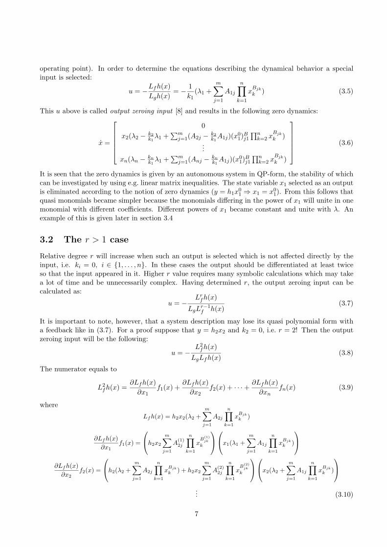
operating point). In order to determine the equations describing the dynamical behavior a specialinput is selected:

u = −Lfh(x)

Lgh(x)= −

1

k1(λ1 +

m∑

j=1

A1j

n∏

k=1

xBjk

k ) (3.5)

This u above is called output zeroing input [8] and results in the following zero dynamics:

x =

0

x2(λ2 −k2k1

λ1 +∑m

j=1(A2j −k2k1

A1j)(x01)

Bj1

∏nk=2 x

Bjk

k )...

xn(λn − kn

k1λ1 +

∑mj=1(Anj −

kn

k1A1j)(x

01)

Bj1

∏nk=2 x

Bjk

k )

(3.6)

It is seen that the zero dynamics is given by an autonomous system in QP-form, the stability of whichcan be investigated by using e.g. linear matrix inequalities. The state variable x1 selected as an outputis eliminated according to the notion of zero dynamics (y = h1x

01 ⇒ x1 = x0

1). From this follows thatquasi monomials became simpler because the monomials differing in the power of x1 will unite in onemonomial with different coefficients. Different powers of x1 became constant and unite with λ. Anexample of this is given later in section 3.4

3.2 The r > 1 case

Relative degree r will increase when such an output is selected which is not affected directly by theinput, i.e. ki = 0, i ∈ {1, . . . , n}. In these cases the output should be differentiated at least twiceso that the input appeared in it. Higher r value requires many symbolic calculations which may takea lot of time and be unnecessarily complex. Having determined r, the output zeroing input can becalculated as:

u = −Lr

fh(x)

LgLr−1f h(x)

(3.7)

It is important to note, however, that a system description may lose its quasi polynomial form witha feedback like in (3.7). For a proof suppose that y = h2x2 and k2 = 0, i.e. r = 2! Then the outputzeroing input will be the following:

u = −L2

fh(x)

LgLfh(x)(3.8)

The numerator equals to

L2fh(x) =

∂Lfh(x)

∂x1f1(x) +

∂Lfh(x)

∂x2f2(x) + · · · +

∂Lfh(x)

∂xnfn(x) (3.9)

where

Lfh(x) = h2x2(λ2 +

m∑

j=1

A2j

n∏

k=1

xBjk

k )

∂Lfh(x)

∂x1f1(x) =

h2x2

m∑

j=1

A(1)2j

n∏

k=1

xB

(1)jk

k

x1(λ1 +

m∑

j=1

A1j

n∏

k=1

xBjk

k )

∂Lfh(x)

∂x2f2(x) =

h2(λ2 +

m∑

j=1

A2j

n∏

k=1

xBjk

k ) + h2x2

m∑

j=1

A(2)2j

n∏

k=1

xB

(2)jk

k

x2(λ2 +

m∑

j=1

A1j

n∏

k=1

xBjk

k )

... (3.10)

7

∂Lfh(x)

∂xn=

h2x2

m∑

j=1

A(n)2j

n∏

k=1

xB

(n)jk

k

xn(λn +

m∑

j=1

A1j

n∏

k=1

xBjk

k )

The notations A(i)2j and B

(i)jk , i = 1, . . . , n are defined as follows:

A(i)2j =

{

0 , Bji = 0A2jBji , Bji 6= 0

, B(i)jk

{

Bjk , k 6= i

Bjk − 1 , k = i(3.11)

Because new coefficient and power matrices are defined, new quasi monomials appear and will remainin the equations after feedback.

Considering the denominator of u we obtain

LgLfh(x) =

h2x2

m∑

j=1

A(1)2j

n∏

k=1

xB

(1)jk

k

x1k1+ (3.12)

+

h2x2

m∑

j=1

A(3)2j

n∏

k=1

xB

(3)jk

k

x3k3 + . . . +

h2x2

m∑

j=1

A(n)2j

n∏

k=1

xB

(n)jk

k

xnkn

it can be seen that the system will remain in quasi polynomial form only when the denominatorcontains only one quasi monomial. Otherwise, it will lose this property.

3.3 Stability analysis of LILO QP systems

Stability is a well-known system property. As mentioned earlier, its analysis may suffer from com-putational difficulties in the case of nonlinear systems. However, there are system classes where theproblem of stability analysis can be solved, e.g. [2], [5] or [6]. For quasi polynomial systems a realiza-tion independent matrix is used in the analysis. Such a matrix is M = BA, see eq. (2.4), which hasdimension m × m, where m equals to the number of quasi monomials.

Local stability analysis can be performed the same way as in linear system theory. At first, anequilibrium point x0 is calculated, and from this, steady state values of the quasi monomials (z0).Then, the matrix

M0 = diag(z0)M =

z01 0 · · · 00 z0

2 · · · 0...

0 0 · · · z0m

M (3.13)

plays the role of the state matrix of a linear time invariant (LTI) system (the linear equivalent off(x)). Stability analysis can be done with the help of the eigenvalues of M0. If the real parts of alleigenvalues are less than 0, i.e. ℜ(si) < 0, i = 1, . . . , m, then the system is asymptotically stable in aneighborhood of x0.

The same can be performed for the zero dynamics (3.6). In this case the dimension of Azd andBzd is smaller than the original of A and B was. However, some quasi monomials become constant,and with their coefficient they unite with λ resulting λzd. From this follows that neither general formfor Azd and Bzd nor general conclusion for the stability of an equilibrium point in the zero dynamics,which was stable before feedback, can be drawn. This property depends on many parameters andfrom this follows that it will not necessarily remain.

8

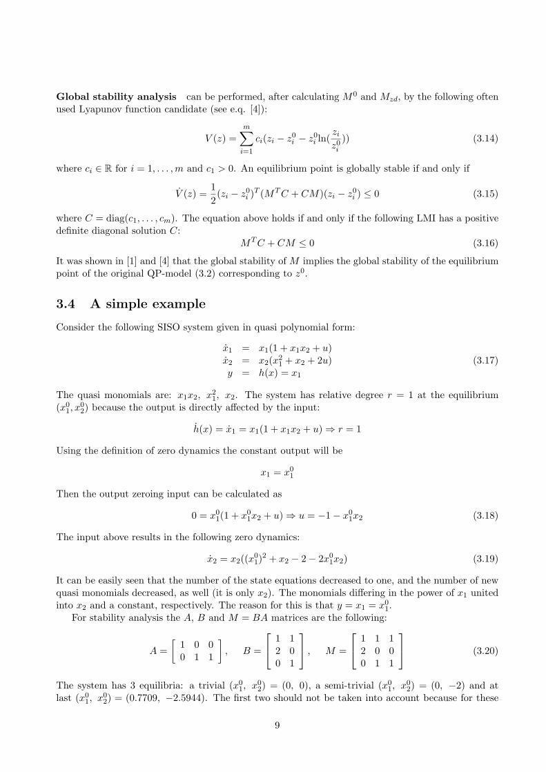
Global stability analysis can be performed, after calculating M0 and Mzd, by the following oftenused Lyapunov function candidate (see e.q. [4]):

V (z) =

m∑

i=1

ci(zi − z0i − z0

i ln(zi

z0i

)) (3.14)

where ci ∈ R for i = 1, . . . , m and c1 > 0. An equilibrium point is globally stable if and only if

V (z) =1

2(zi − z0

i )T (MT C + CM)(zi − z0i ) ≤ 0 (3.15)

where C = diag(c1, . . . , cm). The equation above holds if and only if the following LMI has a positivedefinite diagonal solution C:

MT C + CM ≤ 0 (3.16)

It was shown in [1] and [4] that the global stability of M implies the global stability of the equilibriumpoint of the original QP-model (3.2) corresponding to z0.

3.4 A simple example

Consider the following SISO system given in quasi polynomial form:

x1 = x1(1 + x1x2 + u)x2 = x2(x

21 + x2 + 2u)

y = h(x) = x1

(3.17)

The quasi monomials are: x1x2, x21, x2. The system has relative degree r = 1 at the equilibrium

(x01, x

02) because the output is directly affected by the input:

h(x) = x1 = x1(1 + x1x2 + u) ⇒ r = 1

Using the definition of zero dynamics the constant output will be

x1 = x01

Then the output zeroing input can be calculated as

0 = x01(1 + x0

1x2 + u) ⇒ u = −1 − x01x2 (3.18)

The input above results in the following zero dynamics:

x2 = x2((x01)

2 + x2 − 2 − 2x01x2) (3.19)

It can be easily seen that the number of the state equations decreased to one, and the number of newquasi monomials decreased, as well (it is only x2). The monomials differing in the power of x1 unitedinto x2 and a constant, respectively. The reason for this is that y = x1 = x0

1.For stability analysis the A, B and M = BA matrices are the following:

A =

[

1 0 00 1 1

]

, B =

1 12 00 1

, M =

1 1 12 0 00 1 1

(3.20)

The system has 3 equilibria: a trivial (x01, x0

2) = (0, 0), a semi-trivial (x01, x0

2) = (0, −2) and atlast (x0

1, x02) = (0.7709, −2.5944). The first two should not be taken into account because for these

9

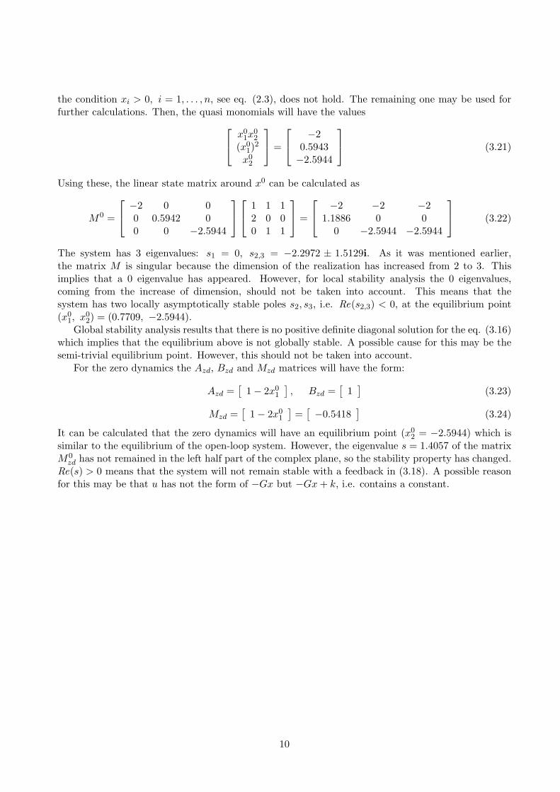
the condition xi > 0, i = 1, . . . , n, see eq. (2.3), does not hold. The remaining one may be used forfurther calculations. Then, the quasi monomials will have the values

x01x

02

(x01)

2

x02

=

−20.5943−2.5944

(3.21)

Using these, the linear state matrix around x0 can be calculated as

M0 =

−2 0 00 0.5942 00 0 −2.5944

1 1 12 0 00 1 1

=

−2 −2 −21.1886 0 0

0 −2.5944 −2.5944

(3.22)

The system has 3 eigenvalues: s1 = 0, s2,3 = −2.2972 ± 1.5129i. As it was mentioned earlier,the matrix M is singular because the dimension of the realization has increased from 2 to 3. Thisimplies that a 0 eigenvalue has appeared. However, for local stability analysis the 0 eigenvalues,coming from the increase of dimension, should not be taken into account. This means that thesystem has two locally asymptotically stable poles s2, s3, i.e. Re(s2,3) < 0, at the equilibrium point(x0

1, x02) = (0.7709, −2.5944).

Global stability analysis results that there is no positive definite diagonal solution for the eq. (3.16)which implies that the equilibrium above is not globally stable. A possible cause for this may be thesemi-trivial equilibrium point. However, this should not be taken into account.

For the zero dynamics the Azd, Bzd and Mzd matrices will have the form:

Azd =[

1 − 2x01

]

, Bzd =[

1]

(3.23)

Mzd =[

1 − 2x01

]

=[

−0.5418]

(3.24)

It can be calculated that the zero dynamics will have an equilibrium point (x02 = −2.5944) which is

similar to the equilibrium of the open-loop system. However, the eigenvalue s = 1.4057 of the matrixM0

zd has not remained in the left half part of the complex plane, so the stability property has changed.Re(s) > 0 means that the system will not remain stable with a feedback in (3.18). A possible reasonfor this may be that u has not the form of −Gx but −Gx + k, i.e. contains a constant.

10

Chapter 4

Case study: heat exchanger cells

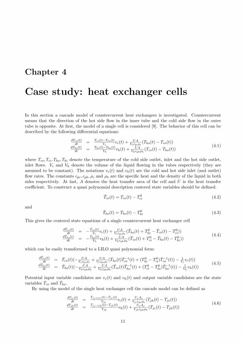
In this section a cascade model of countercurrent heat exchangers is investigated. Countercurrentmeans that the direction of the hot side flow in the inner tube and the cold side flow in the outertube is opposite. At first, the model of a single cell is considered [9]. The behavior of this cell can bedescribed by the following differential equations:

dTco(t)dt

= Tci(t)−Tco(t)Vc

vc(t) + UAVccpcρc

(Tho(t) − Tco(t))dTho(t)

dt= Thi(t)−Tho(t)

Vhvh(t) + UA

Vhcphρh(Tco(t) − Tho(t))

(4.1)

where Tco, Tci, Tho, Thi denote the temperature of the cold side outlet, inlet and the hot side outlet,inlet flows. Vc and Vh denote the volume of the liquid flowing in the tubes respectively (they areassumed to be constant). The notations vc(t) and vh(t) are the cold and hot side inlet (and outlet)flow rates. The constants cpc, cph, ρc and ρh are the specific heat and the density of the liquid in bothsides respectively. At last, A denotes the heat transfer area of the cell and U is the heat transfercoefficient. To construct a quasi polynomial description centered state variables should be defined:

Tco(t) = Tco(t) − T 0ci (4.2)

andTho(t) = Tho(t) − T 0

hi (4.3)

This gives the centered state equations of a single countercurrent heat exchanger cell

dTco(t)dt

= − Tco(t)Vc

vc(t) + UAVccpcρc

(Tho(t) + T 0hi − Tco(t) − T 0

ci))dTho(t)

dt= − Tho(t)

Vhvh(t) + UA

Vhcphρh(Tco(t) + T 0

ci − Tho(t) − T 0hi))

(4.4)

which can be easily transformed to a LILO quasi polynomial form:

dTco(t)dt

= Tco(t)(−UA

Vccpcρc+ UA

Vccpcρc(Tho(t)T

−1co (t) + (T 0

hi − T 0ci)T

−1co (t)) − 1

Vcvc(t))

dTho(t)dt

= Tho(t)(−UA

Vhcphρh+ UA

Vhcphρh(Tco(t)T

−1ho (t) + (T 0

ci − T 0hi)T

−1ho (t)) − 1

Vhvh(t))

(4.5)

Potential input variable candidates are vc(t) and vh(t) and output variable candidates are the statevariables Tco and Tho.

By using the model of the single heat exchanger cell the cascade model can be defined as

dTjc(t)dt

=T(j+1)c(t)−Tjc(t)

Vjcvc(t) +

UjAj

Vjccpcρc(Tjh(t) − Tjc(t))

dTjh(t)dt

=T(j−1)h(t)−Tjh(t)

Vjhvh(t) +

UjAj

Vjhcphρh(Tjc(t) − Tjh(t))

(4.6)

11

where j = 1, . . . , n and Tn+1c = Tci, T1c = Tco, T0h = Thi, Tnh = Tho.According to the centered model in eq. (4.4) the same can be drawn for eq. (4.6):

dTjc(t)dt

= Tjc(t)(−UjAj

Vjccpcρc+

UjAj

Vjccpcρc(Tjh(t)T−1

jc (t) + (T 0(j−1)h − T 0

(j+1)c)T−1jc (t)) − 1

Vjcvc(t))

dTjh(t)dt

= Tjh(t)(−UjAj

Vjhcphρh+

UjAj

Vjhcphρh(Tjc(t)T

−1jh (t) + (T 0

(j+1)c − T 0(j−1)h)T−1

jh (t)) − 1Vjh

vh(t))

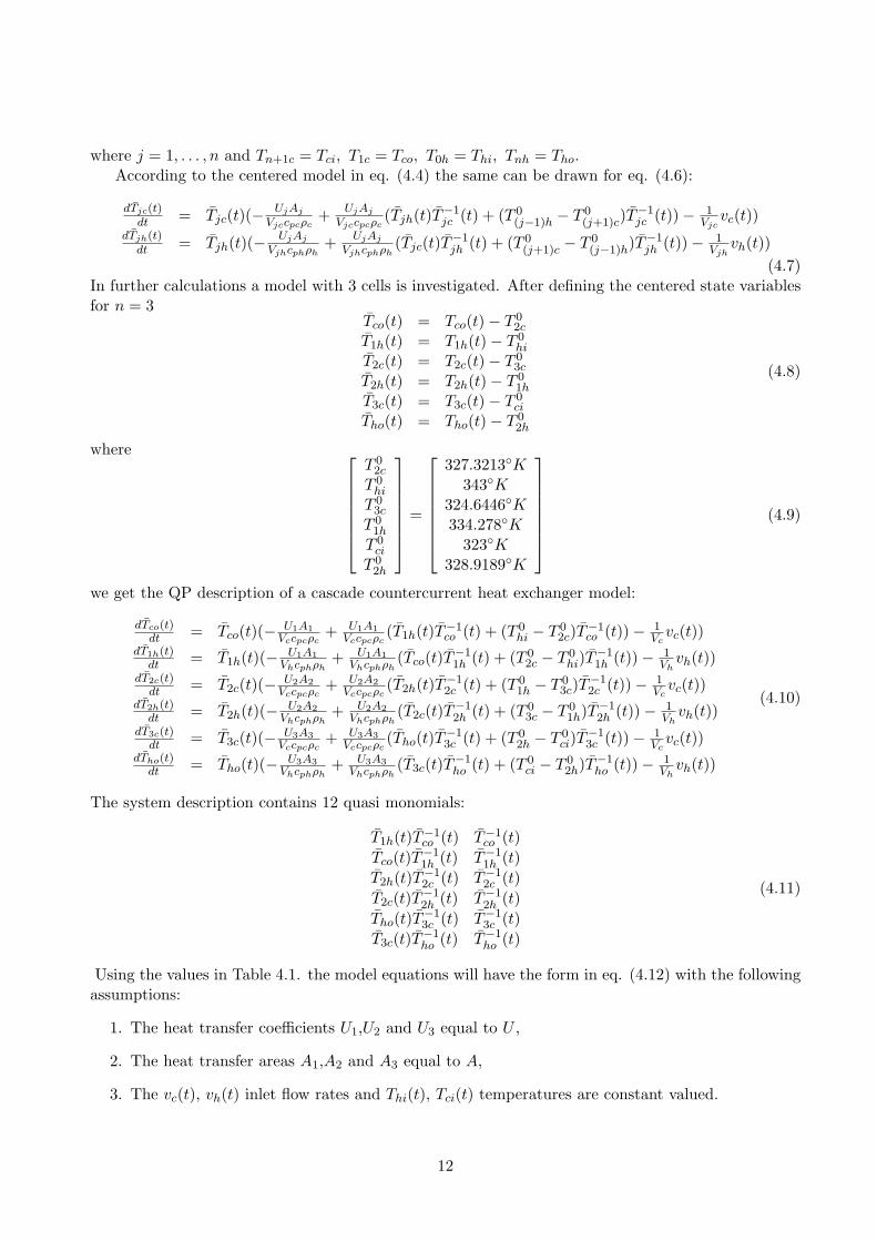
(4.7)In further calculations a model with 3 cells is investigated. After defining the centered state variablesfor n = 3

Tco(t) = Tco(t) − T 02c

T1h(t) = T1h(t) − T 0hi

T2c(t) = T2c(t) − T 03c

T2h(t) = T2h(t) − T 01h

T3c(t) = T3c(t) − T 0ci

Tho(t) = Tho(t) − T 02h

(4.8)

where

T 02c

T 0hi

T 03c

T 01h

T 0ci

T 02h

=

327.3213◦K343◦K

324.6446◦K334.278◦K

323◦K328.9189◦K

(4.9)

we get the QP description of a cascade countercurrent heat exchanger model:

dTco(t)dt

= Tco(t)(−U1A1

Vccpcρc+ U1A1

Vccpcρc(T1h(t)T−1

co (t) + (T 0hi − T 0

2c)T−1co (t)) − 1

Vcvc(t))

dT1h(t)dt

= T1h(t)(− U1A1Vhcphρh

+ U1A1Vhcphρh

(Tco(t)T−11h (t) + (T 0

2c − T 0hi)T

−11h (t)) − 1

Vhvh(t))

dT2c(t)dt

= T2c(t)(−U2A2

Vccpcρc+ U2A2

Vccpcρc(T2h(t)T−1

2c (t) + (T 01h − T 0

3c)T−12c (t)) − 1

Vcvc(t))

dT2h(t)dt

= T2h(t)(− U2A2Vhcphρh

+ U2A2Vhcphρh

(T2c(t)T−12h (t) + (T 0

3c − T 01h)T−1

2h (t)) − 1Vh

vh(t))dT3c(t)

dt= T3c(t)(−

U3A3Vccpcρc

+ U3A3Vccpcρc

(Tho(t)T−13c (t) + (T 0

2h − T 0ci)T

−13c (t)) − 1

Vcvc(t))

dTho(t)dt

= Tho(t)(−U3A3

Vhcphρh+ U3A3

Vhcphρh(T3c(t)T

−1ho (t) + (T 0

ci − T 02h)T−1

ho (t)) − 1Vh

vh(t))

(4.10)

The system description contains 12 quasi monomials:

T1h(t)T−1co (t) T−1

co (t)

Tco(t)T−11h (t) T−1

1h (t)

T2h(t)T−12c (t) T−1

2c (t)

T2c(t)T−12h (t) T−1

2h (t)

Tho(t)T−13c (t) T−1

3c (t)

T3c(t)T−1ho (t) T−1

ho (t)

(4.11)

Using the values in Table 4.1. the model equations will have the form in eq. (4.12) with the followingassumptions:

1. The heat transfer coefficients U1,U2 and U3 equal to U ,

2. The heat transfer areas A1,A2 and A3 equal to A,

3. The vc(t), vh(t) inlet flow rates and Thi(t), Tci(t) temperatures are constant valued.

12

U heat transfer coefficient 400 Wm2K

A heat transfer area 4 m2

Vc volume of the cold side liquid 1 m3

Vh volume of the hot side liquid 0.5 m3

cpc specific heat of the cold side liquid 1910 JkgK

cph specific heat of the hot side liquid 1590 JkgK

ρc density of the cold side liquid 1000 kgm3

ρh density of the hot side liquid 1000 kgm3

vc cold side flow rate 0.0005 m3

s

vh hot side flow rate 0.0003 m3

s

Tci temperature of the cold side inlet flow rate 323 K

Thi temperature of the hot side inlet flow rate 343 K

Table 4.1: Parameter values and dimensions in the cascade model

dTco(t)dt

= Tco(t)(−0.0013 + 0.0008T1h(t)T−1co (t) + 0.0131T−1

co (t))dT1h(t)

dt= T1h(t)(−0.0026 + 0.002Tco(t)T

−11h (t) − 0.0315T−1

1h (t))dT2c(t)

dt= T2c(t)(−0.0013 + 0.0008T2h(t)T−1

2c (t) + 0.008T−12c (t))

dT2h(t)dt

= T2h(t)(−0.0026 + 0.002T2c(t)T−12h (t) − 0.0193T−1

2h (t))dT3c(t)

dt= T3c(t)(−0.0013 + 0.0008Tho(t)T

−13c (t) + 0.0049T−1

3c (t))dTho(t)

dt= Tho(t)(−0.0026 + 0.002T3c(t)T

−1ho (t) − 0.0119T−1

ho (t))

(4.12)

The system above has only one equilibrium point, which can be calculated easily, and takes thefollowing values:

Tco

T1h

T2c

T2h

T3c

Tho

=

4.3564◦K−8.722◦K2.6767◦K−5.359◦K1.6446◦K−3.2926◦K

(4.13)

Local stability requires the determination of M which depends on A and B. The matrix diag(z0)Mhas 12 eigenvalues from which 6 equal to 0. According to the principles in Section 2. these shouldnot be taken into account. The remaining ones have negative real parts which means that the systemis locally asymptotically stable, moreover global, because there is only one equilibrium point in thesystem.

4.1 The r = 1 case

Choosing vc(t) as an input and Tco as an output, the system will have relative degree 1 in a neighbor-hood of Tco = T 0

co. The output zeroing input can be calculated as

vc(t) = −U1A1

cpcρc+

U1A1

cpcρc

(

1

T 0co

T1h(t) +T 0

hi − T 02c

T 0co

)

(4.14)

13

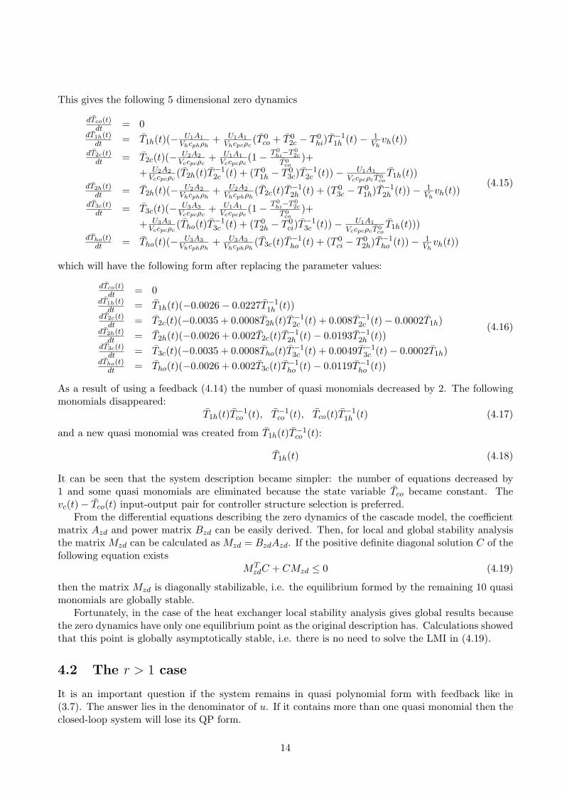
This gives the following 5 dimensional zero dynamics

dTco(t)dt

= 0dT1h(t)

dt= T1h(t)(− U1A1

Vhcphρh+ U1A1

Vhcpcρc(T 0

co + T 02c − T 0

hi)T−11h (t) − 1

Vhvh(t))

dT2c(t)dt

= T2c(t)(−U2A2

Vccpcρc+ U1A1

Vccpcρc(1 −

T 0hi−T 0

2c

T 0co

)+

+ U2A2Vccpcρc

(T2h(t)T−12c (t) + (T 0

1h − T 03c)T

−12c (t)) − U1A1

VccpcρcT 0co

T1h(t))dT2h(t)

dt= T2h(t)(− U2A2

Vhcphρh+ U2A2

Vhcphρh(T2c(t)T

−12h (t) + (T 0

3c − T 01h)T−1

2h (t)) − 1Vh

vh(t))

dT3c(t)dt

= T3c(t)(−U3A3

Vccpcρc+ U1A1

Vccpcρc(1 −

T 0hi−T 0

2c

T 0co

)+

+ U3A3Vccpcρc

(Tho(t)T−13c (t) + (T 0

2h − T 0ci)T

−13c (t)) − U1A1

VccpcρcT 0co

T1h(t)))dTho(t)

dt= Tho(t)(−

U3A3Vhcphρh

+ U3A3Vhcphρh

(T3c(t)T−1ho (t) + (T 0

ci − T 02h)T−1

ho (t)) − 1Vh

vh(t))

(4.15)

which will have the following form after replacing the parameter values:

dTco(t)dt

= 0dT1h(t)

dt= T1h(t)(−0.0026 − 0.0227T−1

1h (t))dT2c(t)

dt= T2c(t)(−0.0035 + 0.0008T2h(t)T−1

2c (t) + 0.008T−12c (t) − 0.0002T1h)

dT2h(t)dt

= T2h(t)(−0.0026 + 0.002T2c(t)T−12h (t) − 0.0193T−1

2h (t))dT3c(t)

dt= T3c(t)(−0.0035 + 0.0008Tho(t)T

−13c (t) + 0.0049T−1

3c (t) − 0.0002T1h)dTho(t)

dt= Tho(t)(−0.0026 + 0.002T3c(t)T

−1ho (t) − 0.0119T−1

ho (t))

(4.16)

As a result of using a feedback (4.14) the number of quasi monomials decreased by 2. The followingmonomials disappeared:

T1h(t)T−1co (t), T−1

co (t), Tco(t)T−11h (t) (4.17)

and a new quasi monomial was created from T1h(t)T−1co (t):

T1h(t) (4.18)

It can be seen that the system description became simpler: the number of equations decreased by1 and some quasi monomials are eliminated because the state variable Tco became constant. Thevc(t) − Tco(t) input-output pair for controller structure selection is preferred.

From the differential equations describing the zero dynamics of the cascade model, the coefficientmatrix Azd and power matrix Bzd can be easily derived. Then, for local and global stability analysisthe matrix Mzd can be calculated as Mzd = BzdAzd. If the positive definite diagonal solution C of thefollowing equation exists

MTzdC + CMzd ≤ 0 (4.19)

then the matrix Mzd is diagonally stabilizable, i.e. the equilibrium formed by the remaining 10 quasimonomials are globally stable.

Fortunately, in the case of the heat exchanger local stability analysis gives global results becausethe zero dynamics have only one equilibrium point as the original description has. Calculations showedthat this point is globally asymptotically stable, i.e. there is no need to solve the LMI in (4.19).

4.2 The r > 1 case

It is an important question if the system remains in quasi polynomial form with feedback like in(3.7). The answer lies in the denominator of u. If it contains more than one quasi monomial then theclosed-loop system will lose its QP form.

14

When vc(t) is the input of the system and Tho is selected as in output then the relative degree ofthe system will be 2. In this case it is easy to see that the condition above does not hold so the systemwill not remain in quasi polynomial form.

15

Chapter 5

Conclusions

Quasi polynomial (QP) form can help in investigating key dynamical properties, such as zero dynamicsof nonlinear systems.

For QP systems with relative degree r = 1 a simple closed formulae is proposed to calculate itszero dynamics. It is shown that the zero dynamics is in QP form and the description is simpler(with fewer quasi monomials). Thus the input-output pairs with r = 1 are always preferable forcontroller structure selections. However, in most cases when r > 1 the QP property may disappearwhen applying output zeroing feedback.

A countercurrent heat exchanger with three cells was investigated for a fixed input and differentoutput selections. In the r = 1 case the closed formulae was used to determine the zero dynamics ofthe system. The QP form became simpler and the number of quasi monomials decreased. For r > 1the condition of remaining in QP form did not hold.

Stability analysis showed for the r = 1 case that not even the original system was globally asymp-totically stable around the equilibrium but the zero dynamics.

16

Bibliography

[1] T.M. Rocha Filho A. Figueiredo, I.M. Gleria. Boundedness of solutions and lyapunov functions inquasi-polynomial systems. Physics Letters A, 286:335–341, 2000.

[2] V. Fairen B. Hernandez-Bermejo. Lotka–volterra representation of general nonlinear systems.Mathematical Biosciences, 140:1–32, 1997.

[3] C. I. Byrnes and A. Isidori. Asymptotic stabilization of minimum-phase nonlinear systems. IEEETransactions on Automatic Control, AC-36:1122–1137, 1991.

[4] B. Hernandez-Bermejo. Stability conditions and liapunov functions for quasi-polynomial systems.Applied Mathematics Letters, 15:25–28, 2002.

[5] A.I. van der Schaft H.Nijmeijer. Nonlinear Dynamical Control Systems. Springer-Verlag, Berlin,1991.

[6] T.M. Rocha Filho I.M. Gleria, A. Figueiredo. On the stability of a class of general non-linearsystems. Physics Letters A, 291:11–16, 2001.

[7] T.M. Rocha Filho I.M. Gleria, A. Figueiredo. A numerical method for the stability analysis ofquasi–polynomial vector fields. Nonlinear Analysis, 52:329–342, 2003.

[8] Alberto Isidori. Nonlinear Control Systems. Springer, Berlin, 1995.

[9] Gabor Szederkenyi. Grey-box approach for the diagnosis, analysis and control of nonlinear processsystems. PhD thesis, University of Veszprem, 2002.

17