Working Paper N 94 | 2021 - bcra.gov.ar

Working Paper N 94 | 2021Inter-provincial Trade in Argentina:Financial Flows and Centralism

Economic ResearchWorking Papers | 2021 | N 94

Inter-provincial Trade in Argentina: Financial Flowsand Centralism

Pedro EloseguiBanco Central de la República Argentina

Marcos Herrera-GómezCONICET-IELDEUniversidad Nacional de Salta

Jorge ColinaInstituto para el Desarrollo Social Argentino

July 2021

2 | BCRA | Working Papers 2017

Working Papers, N 94

Inter-provincial Trade in Argentina: Financial Flows and Centralism

Pedro EloseguiBanco Central de la República Argentina

Marcos Herrera-GómezCONICET-IELDEUniversidad Nacional de Salta

Jorge ColinaInstituto para el Desarrollo Social Argentino

July 2021ISSN 1850-3977Electronic Edition

Reconquista 266, C1003ABFCiudad Autónoma de Buenos Aires, ArgentinaPhone | 54 11 4348-3582Email | [email protected] | www.bcra.gob.ar

The opinions expressed in this paper are the sole responsibility of its authors and do not necessarily represent the position of the Central Bank of Argentina. The Working Papers series is comprised of preliminary material intended to stimulate academic debate and receive comments. This paper may not be referenced without authorization from the authors.

NON-TECHNICAL SUMMARY

Research Question

International evidence highlights the relevance of trade not only between countries but alsoat sub-national regions level, particularly in federal countries. Trade is a dynamic ingredientfostering innovation, productivity and economic growth, as well as a key factor (along withfinancial and migration flows) for the transmission of economic shocks. Despite its importance,sub-national trade is rarely included as a central aspect in the economic analysis and, in mostcases, this absence is related to the lack of information. In fact, in our country there is no publicinformation on the flow of trade in goods and services between the provinces. Our work, which ispart of a broader research agenda, analyzes the main determinants of trade between Argentineprovinces using a new database based on fiscal information for the year 2017. The relevanceof trade information between Argentine provinces is analyzed by investigating its importanceas a reflection of commercial and productive interaction. In line with the relevant literature,we evaluate the main potential determinants of trade including the different characteristicsof the markets both at origin and destination, the role of distance as well as unobservablefactors or potential barriers to trade. In this framework, we analyze the impact of the historicalcentrality of the Autonomous City of Buenos Aires and the province of Buenos Aires overbilateral trade between provinces. Likewise, we consider the redistributive financial flows, withinthe framework of the secondary distribution of the co-participation regime. Finally, consideringthat the database includes only registered trade, we analyze the impact of income distributionas well as the use of different means of payments, which show considerable variability betweenprovinces.

Contribution

The work underscore the important value of the unpublished information of inter-provincialtrade in Argentina and highlights the relevance of a systematic calculation of such information.On the other hand, by using novel spatial econometric tools we show the relevance of barriersto inter-provincial trade among the Argentine provinces. Our results allow us to quantify theimpact of the social and economic centralism in the city of Buenos Aires and Buenos AiresProvince, as well as the impact of federal co-participation, income distribution and the use ofalternative means of payments.

Results

The main results of the article are as follows:

i. The main positive determinants of trade between Argentine provinces include the socioeco-nomic activity in the markets of origin and destination, as well as the geographic contiguity.As expected, there is a negative effect of distance as well as border effects that negatively af-fect domestic bilateral trade. The results are similar to those found in the literature in othercountries, which highlights the usefulness of the database under analysis.

ii. The centralism derived from the economic, social and commercial concentration in the Cityof Buenos Aires and Buenos Aires Province discourages bilateral trade between the provincesin the interior of the country.

iii. The financial flows of the co-participation are negatively related to bilateral trade flows,significantly discouraging sales to other provinces from the most lagging provinces. This negative

impact is reinforced by the level of co-participation received by the provinces located in thevicinity of the province of origin.

iv. Inter-provincial trade is negatively influenced by the (poor) distribution of income, affec-ting the poorest provinces. Likewise, formal means of payment affect bilateral trade betweenprovinces, highlighting the positive impact of credit cards.

Inter-provincial trade in Argentina: financial flows and

centralism.∗

Pedro Elosegui†, Marcos Herrera-Gomez‡, and Jorge Colina§

Abstract

This paper is part of a broader agenda and constitutes a first step to empiricallyunderstand the main determinants of the inter-provincial trade in Argentina. We usea novel database of regional trade flows between the 24 Argentinean provinces for 2017.Using a structural gravity model and novel econometric techniques we analyze the mainvariables influencing trade between the provinces. In addition to the traditional variablesof the canonical gravity model we add some variables of interest that ca possible affecttrade between sub national jurisdictions. With an especial focus in financial flows weanalyze the impact of co-participation transfers, income distribution and household’spayment methods, among other variables that may be correlated with formal trade.Additionally, we analyze the potential impact of trade concentration in the AutonomousCity of Buenos Aires (CABA) and Buenos Aires. Trade flows are analyzed consideringboth, origin and destination. The results indicate that national transfers from theredistribution federal arrangement are an important determinant of inter provincial tradegenerating relevant (and negative in the origin) spillover effects between the provinces.Also, the concentration in CABA and Buenos Aires discourages inter-provincial trade.

JEL Classification: R10, F14, C21.

Keywords: Gravity Model, Spatial Interactions, Redistribution Federal Arrangement.

∗A previous version of this research was presented at the 13th World Congress of the Regional ScienceAssociation International (RSAI). We thank valuable comments and suggestions that improved the presentversion. We also thank the COMARB for the data and valuable suggestions from authorities and provincialrepresentatives and an anonymous reviewer for helpful comments.†BCRA, Subgerencia General de Investigaciones Económicas. E-mail: [email protected]. The views

expressed herein are those of the authors and are not necessarily those of the Central Bank of Argentina andits authorities.‡CONICET-IELDE, UNSa. E-mail: [email protected]§IDESA. Institute for the Argentine Social Development. E-mail:[email protected]

1

1 Introduction

The international evidence shows that trade between provinces and sub national regions areeconomically relevant (McCallum, 1995 and Wei, 1996). As emphasized by Álvarez et al.(2018) and as in the case of international trade, economic literature indicates that bilateraltrade is one important driver of productivity, catalysts of innovation and economic growth.Also, there is evidence that shocks originating in regions or provinces can spread at themacroeconomic level through trade flows of inputs, goods and services. Financial flowsand population migration may be relevant and interact with trade flows to spread economicshocks between sub national jurisdictions (Caliendo et al., 2018). 1 The interaction betweenshocks of local and national origin provides relevant information for the implementationof macroeconomic policies, which are usually uniform (“blind”) at the national level, anddesigned based on a set of information that should consider the mentioned transmissionchannels between regions.

Despite its relevance, in our country there are no official statistics on trade betweenprovincial jurisdictions. The countries that have this type of information use surveys orregistries. In some cases, the data are based on transportation surveys (or registries) 2, inother, taxation information is used. 3 In the case of our country, as analyzed by Elosegui &Pinto (2018), the information from the Multilateral Agreement on Gross Income Tax (IIBB),established in art. 9 of the Coparticipation Law, offers a unique opportunity to approximatethe flows of trade in goods and services between the provinces, since it establishes a uniformcriterion for the tax base allocation of provincial turnover tax (IIBB) between the provincialjurisdictions. Based on that methodology and with a more comprehensive national databasefrom the same source, Colina (2019) calculates trade flows for all the provinces in 2017.

In this paper we use that novel database and empirically apply a gravity model to analyzeinter-provincial trade for all provinces during year 2017. We analyze the main determinantsof trade flows between the provinces, adding to a canonical gravity model several variablesthat can possibly affect trade between sub national jurisdictions. We take into account theasymmetric economic structure of the economy, highly concentrated in the Autonomous Cityof Buenos Aires (CABA, from its Spanish initials) and the Buenos Aires province. As we willsee, a long lasting feature, which has not been analyzed yet, considering the role of tradebetween the provinces. In particular, we focus on the impact of financial flows between theprovinces, especially those related to transfers aimed to reduce such asymmetries.

The financial flows and the interaction of those flows with inter-provincial tradeapproximate the relevance of certain regional shocks that can have important consequences

1In fact, Caliendo et al. (2018) indicate that in U.S. the geography of economic activity is actually relevant andthe aggregate economic cost of their estimated domestic trade barriers is large both in GDP and productivityterms. See their Appendix Table A7.2 page 2088.

2Commodity Flow Survey (CFS) in U.S., https://www.census.gov/programs-surveys/cfs.html.3For example, the "Balanca Comercial interestadual" in Brazil, https://www.confaz.fazenda.gov.br/

balanca-comercial-interestadual.

2

at the aggregate level. To understand the scope of these shocks and their spread to therest of the economy, it is necessary not only to quantify the degree of economic and tradeinterrelation between the regions but also to control for the main determinants, includingstructural economic and financial aspects. The greatest limitation, until now, to develop thistask has been the lack of availability of information about inter-provincial trade. Precisely,the type of information that is introduced in this work for the first time for the entire country.It should be noted, that the dataset is based on tax information and it only reflects formaltrade of goods and services. In addition, most (but not all) of the formal trade is transactedtrough formal financial services, including credit transactions. 4

Although regional shocks may not be transferred to the rest of the economy, they mayhave a differential impact on the local economy depending on the economic structure of thedifferent regions or provinces (Blanco et al., 2019). In particular, the database reveals thehigh relative importance of the main jurisdictions of CABA and Buenos Aires, with respectto the rest of the provinces. This relative asymmetry in size and economic diversificationis relevant when considering the potential impact of shocks originating in the provinces,including financial shocks on the economy in general.

The rest of the paper is organized as follows. The second section introduces the mainliterature and the evidence analyzed with similar models in other economies. Resultsindicate the relevance of considering trade between provinces, including the interactionbetween internal trade and fiscal transfers. In the third section, we introduce the noveldata set and describe the concentration of economic and social variables and trade. Sectionfourth introduces the theoretical framework for our empirical application. In the fifth section,the empirical approach is introduced, with the main characteristics of the adaptation ofthe canonical model to the database and the characteristics of the economy under analysis.Section six includes the estimation results and their analysis. Finally, in section seven, weintroduce the main conclusions and the next steps of this research agenda.

2 Literature

Argentina is a federal country characterized by a strong asymmetry in the economicdevelopment of its provinces. This is a long-standing situation and it has been analyzedby prestigious scholars, like Bunge (1940). He described the regions as a “folding fan”, withthe head in Buenos Aires Port (the main center) from which the socioeconomic indicatorsdecreased with distance (see Asiain, 2014). Since the national organization, with theConstitution of 1853 and 1860, fiscal federalism went through several stages until reachingthe current co-participation scheme (Porto, 2018). The current system delimits the fiscalpowers of the provinces and the Nation, establishing a “primary” distribution between

4The extent of informal economy and the use of cash in transactions are correlated and show variationsbetween the provinces (Elosegui et al., 2021).

3

them and then a “secondary” distribution between the provinces. In this scheme, the nationmaintains powers to make certain transfers to the provinces. However, it is the secondarydistribution the one that establishes the main redistributive mechanism from the richest tothe less developed provinces. Also, the provinces keep to themselves the collection of localproperty taxes and the turnover tax, the IIBB (Elosegui & Pinto, 2018). Moreover, as hasbeen emphasized by Porto (2018) and Porto & Elizagaray (2011), the co-participation schemegenerated a relative convergence of different social indicators. However, after many yearsthe asymmetries remain, and the relative increase in co-participation transfers in favor oflagged regions is not reflected in their relative development. The center regions, CABA andBuenos Aires, still hold a dominant position in socio-economic indicators.

In general, economic asymmetries are measured by comparing synthetic indicators suchas per capita GDP or the value added by economic sectors or by using registry information,such formal wages or provincial exports to foreign markets. A complementary alternative tounderstand the profound differences between the provinces is to analyze the internal trade.In our work, we use this novel database to explore the main determinants of asymmetries intrade between provinces. In particular, we empirically analyze the impact derived fromthe financial flows of the co-participation scheme, as well as the effect of the markedcentralization in CABA and Buenos Aires.

Our initial work, within the framework of a more ambitious agenda, contributes anddraws on various related literature. It is the first application to Argentina of the gravityinterprovincial trade model, since it uses a novel database. The setting is related to abroad literature that evaluates the (negative) impact of regional borders on trade flowswithin countries. This literature, with different details on the gravity model approach,include mostly developed federal countries, such as the United States (Head & Mayer,2010; Yilmazkuday, 2012), European countries as Spain (Requena & Llano, 2010) and France(Combes et al., 2005), also Canada (Tombe & Winter, 2021), and China (Poncet, 2005), amongothers. In the region, the empirical applications are scarce, as domestic trade informationis not readily available. Only in the case of Brazil, we can cite the works by Fally et al.(2010) and Daumal & Zignago (2010), both using the same 1999 domestic trade information.This literature analyzes the extent of border effects and domestic bias in internal trade aswell as the internal costs derived from domestic trade barriers, distance and/or asymmetriesbetween provinces. It should be noted, that in federal countries the presence of trade barriersbetween provinces may be a consequence of the multilevel governance system and does notgenerally take the form of explicit tariffs or taxes. However, there may be tax competitionor discriminatory tax treatments of extraterritorial firms, provincial regulations and/orcertifications for local provision of professional services, provincial public procurementregulations that privilege local producers among other factors that potentially generatesome type of border effects between the provinces. Also, the provinces may have different

4

coverage of financial services that can affect bilateral trade between the provinces, such asdifferent access to credit and/or formal means of payments.

Finally, there is a closely related literature focused on the impact of federal transfers overthe provincial and national economic activity using internal bilateral trade. This type ofanalysis is not very extended, as Tombe & Winter (2021) emphasizes the large literatureon the topic, usually “abstracts from trade”. In fact, literature mainly focus on the impactof financial transfers on the incentives of workers to migrate. In their very interesting andcomplete quantitative analysis for Canada, the authors incorporate internal trade to quantifythe impact of fiscal financial transfers over provincial and national activity. In the particularcase of Canada, they find no evidence that fiscal transfers affect the estimated presence oftrade costs and border effects between provinces. However, they uncover an importantimpact of fiscal transfers on trade flows.

3 Dataset

The dataset on internal provincial trade is novel, unpublished and calculated from taxrecords. The original data comes from the Multilateral Agreement on Provincial GrossIncome Tax managed by the Arbitrational Commision (COMARB). 5 This information, basedon the provincial turnover sales tax, was processed, as reflected in Colina (2019) and Elosegui& Pinto (2018), to calculate exports and imports of goods and services (including thosereached by the aforementioned inter-provincial agreement) between the 24 provinces ofArgentina for year 2017. To this novel matrix of trade among provinces we added thewithin jurisdiction sales (also coming from provincial turnover tax collections) to have acomplete cross section of sales within and between provinces. It should be noted that thetax information is reflecting formal transactions. Most of these declared sales come from theautomatic retention schemes that operate through the formal financial channels. It shouldalso be noted that provinces have incentives to cross audit and control tax evasion, underreporting and potential fiscal base hoarding arising from non uniform fiscal treatments(Arias, 2011). In fact, there have been substantial progress lately to harmonize the scopeof the tax which is auspicious for future processing of this database. As we will show, resultsremark the relevance of this internal trade information for both national and provincialeconomic decision making process.

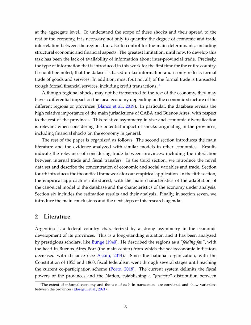
Figure 1 summarizes the geographical distribution of provincial population andeconomic activity in Argentina. It should be noted that Ciudad Autonoma of Buenos Aires(CABA) (zoomed in a the box) and Buenos Aires province both located at the middle eastarea of the country are the main economic and social centers. As mentioned before these

5The Comisión Arbitral del Convenio Multilateral de Impuesto a los Ingresos Brutos (COMARB) is a federalentity managed by the provinces with the "spirit of ordering the exercise of concurrent tax powers" betweenthe jurisdictions, and to prevent multiple taxation through the distribution of taxable base of the Gross IncomeProvincial Tax.

5

social indicators tend to decrease in value for the peripheral provinces, as the distance fromthe center increases.

Figure 1: Geographical distribution of GDP and population (in percentage).

As can be seen in Figure 2, internal trade among provinces is also highly concentratedin CABA and Buenos Aires, practically a mirror of economic and social concentration. Ineffect, approximately 60% of total internal trade, including both trade within and betweenprovinces is concentrated in these two provinces. Also, the other two largest provincialeconomies of the interior of the country Cordoba and Santa Fe show an important level oftrade with the rest of the provinces. Indeed, concentration is not too far from the figure usedby Bunge (1940), to the extent that the center and the nearby provinces, richer and morepopulated, are the ones concentrating most of the domestic trade. 6

As we will show in the econometric model, inter-provincial trade shows correlation withmarket dynamics. Therefore, it is interesting to consider a relative measure of bilateral tradebetween the provinces, such as the localization coefficient. Figure 3 shows internal tradeamong provinces as measured by the coefficient of localization LQi for province i, given by:

LQi = (Ti/GDPi)(GDPi/GDP ) , (1)

where Ti and GDPi capture the total interprovincial trade and the gross domestic productfor the province i, respectively; with GDP as the total sum provincial products.

6In the Appendix, Table A summarizes the provincial comparison in terms of GDP and Population (%) andTable C indicates the average trade between provinces, including internal transactions (%).

6

Figure 2: Internal trade among provinces

The internal trade is important for Neuquén and Tierra del Fuego, the two provinces withLQ > 1. In the first case, the coefficient is reflecting the important trade of energy resources.In the second case, it is related to the industrial promotion regime of the province, and alsothe fact that Tierra del Fuego is actually an island. The coefficient is lower than one for allthe other provinces indicating that internal bilateral trade seems not to be actually importantfor the provinces.

Figure 3: Coefficient of localization of provinces

7

In addition to the internal trade information, we use data from the National HouseholdSurvey (ENGHO) of 2017/2018 to measure the extent of the informal economy and the useof formal and informal payments methods by province. In the first case, we calculate themean income by the two lowest decile to approximate for the informality level at provinciallevel. In the second case, as proxy for the use of financial services we consider the share ofhousehold cash and credit expenditure in each province. Finally, information on provincialGDP and population is from INDEC whereas the co-participation data comes from theNational Ministry of Finance.

4 Theoretical framework

Our theoretical framework is based on the gravity equation, one of the main econometrictechnique used by the literature to analyze the bilateral trade and economic factors(Anderson & Van Wincoop, 2003). The model captures the notion that the bilateral tradeflow (Tij) is determined by important factors related to market dynamics such as the sizeof the region i and j, typically measured by the gross domestic product (GDP ), or regionalincome, and the geographical distance between regions (Tinbergen, 1962):

Tij =GDP β1

i ×GDP β2j

Distγij. (2)

In the literature of regional science, the gravity model has been labelled a spatialinteraction model (Sen & Smith, 1995) and it tries to explain the variation in the n2 interactionflows between n regions in a closed regional network. Additionally, the conventional gravitymodel relies on an n × k matrix of explanatory variables that we label X , containing k

characteristics for each of the n regions. The matrix X is repeated n times to produce anN(= n2)×k matrix representing exporting (origin) characteristics that we label Xi. A second

matrix can be formed in similar way to represent importing (destination) characteristicsresulting in an N × k matrix, Xj . Also, different alternatives of distance are used to capturethe resistance or deterrence to flow between regions. Using these extensions and applying alog transformation, the equation (1) can be written in general terms as:

ln T = β0ιN + Xiβi + Xjβj + Dγ + ε, (3)

8

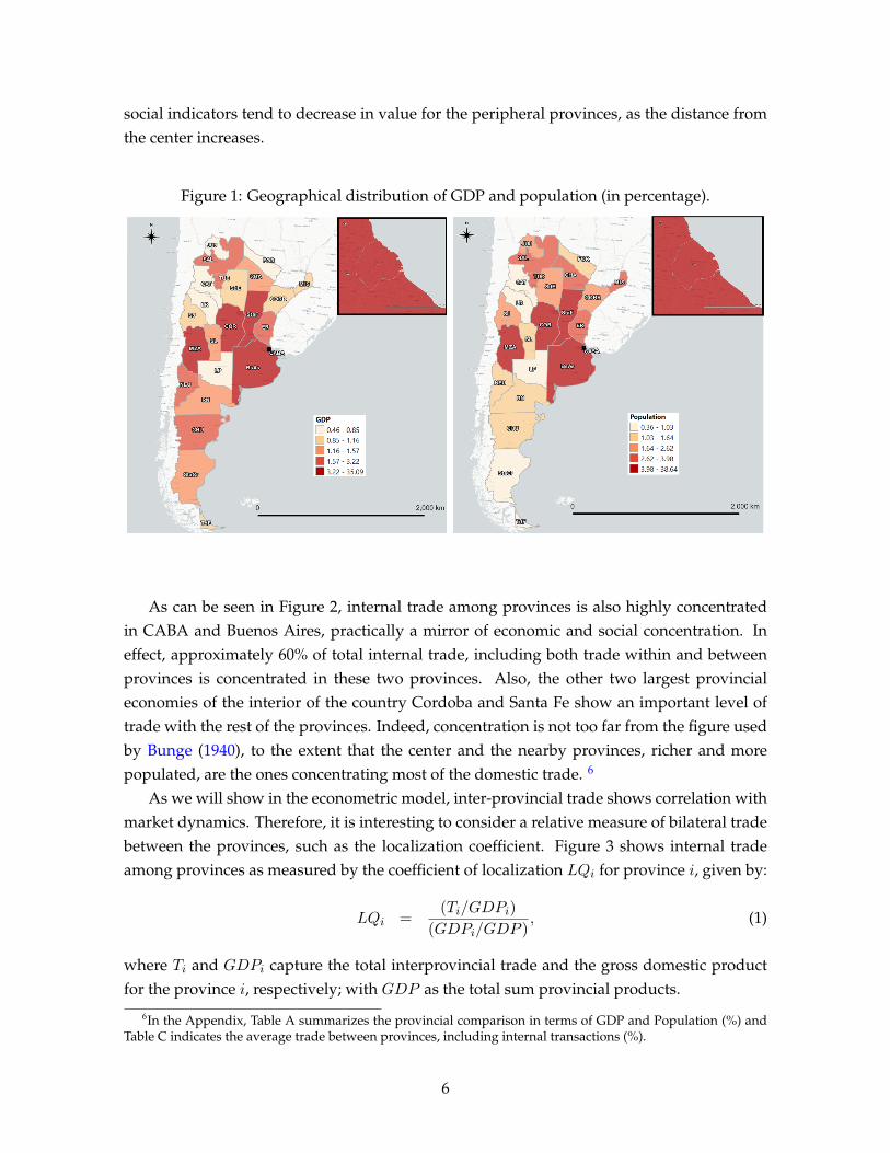
where ln T is an N × 1 vector of logged flows constructed by stacking the columns of then × n flow7; Xi includes lnGDPi, Xj includes lnGDPj , and D includes a function of thegeographical distance and other measures of proximity between regions; ε is anN×1 vectorof error terms with each element independent and identically distributed, i.i.d.

(0, σ2).

The gravity models assume that the use of geographical distance and/or other similarproxies, as explanatory variables can eradicate the spatial dependence of the trade flowsbetween pairs of regions. However, this assumption has long been criticized from theperspective of spatial econometrics. (Fischer & Griffith, 2008; LeSage & Pace, 2008). Indeed,the usual spatial econometric approach captures the spatial dependence in the error termby using spatial weighting structures between the N exporting-importing pairs in a mannerconsistent with the conventional model given by equation (2). Under this perspective, themodel can be transformed in the following spatial econometric exporting-importing flowmodel:

ln T = β0ιN + Xiβi + Xjβj + Dγ + u, (4)

u = λWu + ε,

where W is a spatial weighting matrix that represents anN×N array; λ is a scalar parametercapturing the degree of spatial dependence known as the spatial autoregressive parameterin the literature; u is a N × 1 error vector term and ε is a N × 1 innovation vector withuncorrelated and homoscedastic innovation terms

(0N , σ2IN

).

It should be noted that spatial econometrics introduces the spatial dependence by using aspatial weighting matrix W . The construction of this matrix is something actually importantin the field. By convention, this spatial structure is a positive square matrix of order n. It isusually pre-specified by the researcher, and describes a hypothesis of a particular interactionof the spatial units in the sample (Anselin, 1988). The elements of W , wij , are non-zerowhen the region i and region j are hypothesized to be neighbors, and zero otherwise. Byconvention, the diagonal elements, wii, are equal to zero, that is, the self-neighbor relation isexcluded:

W =

0 w12 · · · w1n

w21 0 · · · w2n...

.... . .

...wn1 w2n · · · 0

. (5)

There are many alternatives to create the spatial matrix W , In fact, it should be observedthat the dimensions of W and W are different. To obtain the W, in this research we followthis sequence of steps:

7Specifically, we apply vec operator such as the model of equation (2) is exporting-centric ordering, know asorigin-centric ordering in the literature of interaction models. See chapter 8 of LeSage & Pace (2009) for moredetails.

9

• First, we create two different matrices using geographical information. The first matrixuses the contiguity criterion (common boundaries) to define the neighbors for eachpolygon (province), Wcont. The second matrix is calculated by using the inverse of thesquared distances, in kilometers, between provincial capital cities, Winv−dist2.

• Second, we combine the two previous matrices into a Wmix, where every weight isthe product of wij, cont × wij, inv−dist2, such as the nearest neighbor (with a commonboundary) is more influential than the other neighbors. Therefore, each weight ofWmix

is defined as:

wij, mix ={

0 if i, j are not contiguous.

d−2ij if i, j are contiguous neighbors

, (6)

where distij is the distance in kilometers between provincial capital cities i and j.

• Finally, we generate two N ×N (n2 × n2) matrices that capture two points of view:

– Wi = Wmix ⊗ In that captures exporting neighborhood dependence.

– Wj = In ⊗Wmix that captures importing neighborhood dependence.

Figure 4 explains the idea of exporting and importing neighborhood and the spatialdependence. For two particular regions, the traditional model uses the information fromregion i (in this case Tucuman) and region j (in this case San Luis), Xi and Xj , to explainthe trade flow (black line). Our spatial econometric extension includes the information fromthe neighborhood region (white regions): Wi is created using the neighborhood of the i− th

region (graph on the left) and Wj is created using the neighborhood of the j − th region(graph on the right).

The weighting matrix for the regression models is row-standardized: the sum ofweights for each row is equal to one. Also, we perform a robustness check by using analternative spatial matrix replacing the contiguity matrix by a 4-nearest neighbors matrix(more information about these alternative results are presented in the appendix).

10

Figure 4: Example of provincial trade and the neighborhood.

Exporting regions (i′s) Importing regions (j′s)

Other important issue related to the possible presence of spatial dependence is thedistinction between origin and destination factors. Under equation (2), we use Moran’s Itest (Moran, 1950) to test the null hypothesis that the error term ε is spatially uncorrelated.When Moran I test is rejected, we explore two specific channels of spatial dependence: (i) alocal spatial dependence through the explanatory variables (WX); and (ii) a global spatialdependence through the error term (Wu). Finally, the model that includes both spatial effectsis known as Spatial Durbin Error Model, SDEM (Elhorst, 2014):

ln T = β0ιN + Xiβi + Xjβj + Dγ + WiXiθi + WjXjθj + u, (7)

u = λWu + ε,

where θi, θj and λ capture the spatial dependence in the explanatory variables (exportingand importing centre) and the error term, respectively; ε is an idiosyncratic innovation termwith each element independent and identically distributed, i.i.d.

(0, σ2). The inclusion of

a spatial error term can help to evaluate the extent of spatial clustering of trade flows thatis not explained by the explanatory variables. In this sense, the coefficient λ captures thespatial effect of unmeasured explanatory variables and the spatial mismatch scale betweenthe different sources of available information (Anselin, 2002). Also, depending on which Wis defined in the error term, we obtain two alternatives SDEM : SDEMexp if the spatial

11

weighting matrix corresponds to the exporting regions (Wi) or SDEMimp if the spatialweighting matrix corresponds to the importing regions (Wj).

Finally, depending on the linear restriction imposed in equation (7), we can obtain aSpatial Lag in X’s model (SLX), with λ = 0:

ln T = β0ιN + Xiβi + Xjβj + Dγ + WiXiθi + WjXjθj + u, (8)

or a Spatial Error Model (SEM ), with θi = θj = 0:

ln T = β0ιN + Xiβi + Xjβj + Dγ + u, (9)

u = λWu + ε,

These nested models are tested in the empirical section using LR tests.

5 Empirical Approach

In the empirical literature, the basic model of equation (2) is commonly augmented to includeadditional control variables of interest for both the exporter and the importer regions. Also,the concept of distance is usually extended to a broader group of trade costs that constitutespotential barriers to trade. Our basic gravity model, in logarithm form, is expressed asfollows:

lnTij = β0 + β1 lnGDPi + β2 lnGDPj + β3CONTIGij + β4 lnDISTij+β5 lnPOPi + β6 lnPOPj + β7 lnCOPAi + β8 lnCOPAj+β9Quantile12i + β10Quantile12j + β11GtoTotCashi + β12GtoTotCashj

+β13GtoTotCredi + β14GtoTotCredj

+β15CABSASij + β16PROV CABSASij + εij , (10)

where the i and j subscripts denote the exporting and importing provinces; Tij (exports plusimports) are the annual average flows between province i and j, including internal tradefor i = j; GDPi and GDPj are the gross domestic product of the exporter and importer,respectively; CONTIGij is a binary variable that indicates whether i and j share a border ornot; DISTij represents the two different bilateral physical distance between provinces i andj.

A summary of the descriptive statistics for the main variables is presented in Table 1. Itshould be noted that, our dependent variable only contains two pairs of flow with zero trade:provinces of Formosa and Chubut, and Formosa and Santa Cruz; then, the potential bias due

12

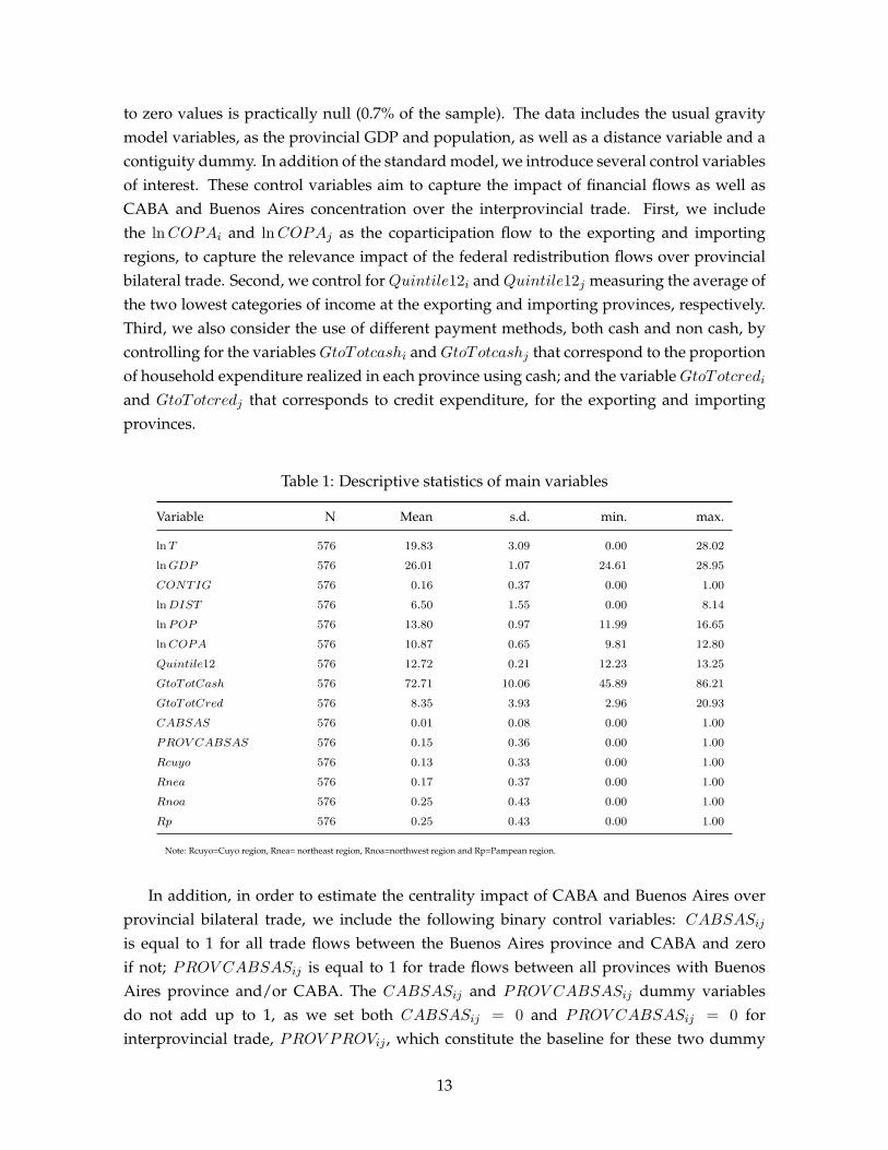
to zero values is practically null (0.7% of the sample). The data includes the usual gravitymodel variables, as the provincial GDP and population, as well as a distance variable and acontiguity dummy. In addition of the standard model, we introduce several control variablesof interest. These control variables aim to capture the impact of financial flows as well asCABA and Buenos Aires concentration over the interprovincial trade. First, we includethe lnCOPAi and lnCOPAj as the coparticipation flow to the exporting and importingregions, to capture the relevance impact of the federal redistribution flows over provincialbilateral trade. Second, we control forQuintile12i andQuintile12j measuring the average ofthe two lowest categories of income at the exporting and importing provinces, respectively.Third, we also consider the use of different payment methods, both cash and non cash, bycontrolling for the variablesGtoTotcashi andGtoTotcashj that correspond to the proportionof household expenditure realized in each province using cash; and the variableGtoTotcrediand GtoTotcredj that corresponds to credit expenditure, for the exporting and importingprovinces.

Table 1: Descriptive statistics of main variables

Variable N Mean s.d. min. max.

lnT 576 19.83 3.09 0.00 28.02lnGDP 576 26.01 1.07 24.61 28.95CONTIG 576 0.16 0.37 0.00 1.00lnDIST 576 6.50 1.55 0.00 8.14lnPOP 576 13.80 0.97 11.99 16.65lnCOPA 576 10.87 0.65 9.81 12.80Quintile12 576 12.72 0.21 12.23 13.25GtoTotCash 576 72.71 10.06 45.89 86.21GtoTotCred 576 8.35 3.93 2.96 20.93CABSAS 576 0.01 0.08 0.00 1.00PROV CABSAS 576 0.15 0.36 0.00 1.00Rcuyo 576 0.13 0.33 0.00 1.00Rnea 576 0.17 0.37 0.00 1.00Rnoa 576 0.25 0.43 0.00 1.00Rp 576 0.25 0.43 0.00 1.00

Note: Rcuyo=Cuyo region, Rnea= northeast region, Rnoa=northwest region and Rp=Pampean region.

In addition, in order to estimate the centrality impact of CABA and Buenos Aires overprovincial bilateral trade, we include the following binary control variables: CABSASijis equal to 1 for all trade flows between the Buenos Aires province and CABA and zeroif not; PROV CABSASij is equal to 1 for trade flows between all provinces with BuenosAires province and/or CABA. The CABSASij and PROV CABSASij dummy variablesdo not add up to 1, as we set both CABSASij = 0 and PROV CABSASij = 0 forinterprovincial trade, PROV PROVij , which constitute the baseline for these two dummy

13

variables. Therefore, a negative coefficient for both dummies would be a sensible test forthe hypothesis that the centrality of CABA and Buenos Aires discourage the interprovincialtrade. Furthermore, as in Daumal & Zignago (2010) the exponential of this estimatedcoefficients reflect the degree of internal fragmentation of Argentina’s internal market.Finally, the εij is the error term with the usual assumption, i.i.d

(0, σ2).

Also, we extend the initial model to include spatial lags in some main variables likelnGDP and lnCOPA. This new model is the SLX version:

lnTij = β0 + β1 lnGDPi + β2 lnGDPj + β3CONTIGij + β4 lnDISTij+β5 lnPOPi + β6 lnPOPj + β7 lnCOPAi + β8 lnCOPAj+β9Quintile12i + β10Quintile12j + β11GtoTotCashi + β12GtoTotCashj

+β13GtoTotCredi + β14GtoTotCredj

+β15CABSASij + β16PROV CABSASij

+β17∑

wiij lnGDPi + β18∑

wjij lnGDPj+β19

∑wiij lnCOPAi + β20

∑wjij lnCOPAj + εij , (11)

Additionally, we explore the SDEMs including a spatial correction in the error term:

lnTij = β0 + β1 lnGDPi + β2 lnGDPj + β3CONTIGij + β4 lnDISTij+β5 lnPOPi + β6 lnPOPj + β7 lnCOPAi + β8 lnCOPAj+β9Quintile12i + β10Quintile12j + β11GtoTotCashi + β12GtoTotCashj

+β13GtoTotCredi + β14GtoTotCredj

+β15CABSASij + β16PROV CABSASij

+β17∑

wiij lnGDPi + β18∑

wjij lnGDPj+β19

∑wiij lnCOPAi + β20

∑wjij lnCOPAj + λ

∑wijuij + εij . (12)

These models are called SDEMexp(Wi

)when the model includes a spatial correction

from exporter’s neighborhood, wiij , and SDEMimp(Wj

)when the model includes a spatial

correction from importer’s neighborhood, wjij .The literature criticizes the gravity models arguing that they do not necessarily capture

the bilateral resistance or border effect terms leading to biased estimates. As a possibleanswer, Feenstra (2002) proposes the inclusion of exporter and importer fixed effects as themost appropriate method. In our models, the inclusion of such fixed effects leads to theexclusion of other variables such as lnGDP and lnCOPA of exporter and importer regions.However, the spatial lags of both variables can be maintained and evaluated in this fixedeffects strategy framework. Therefore, the models for exporter and importers become:

14

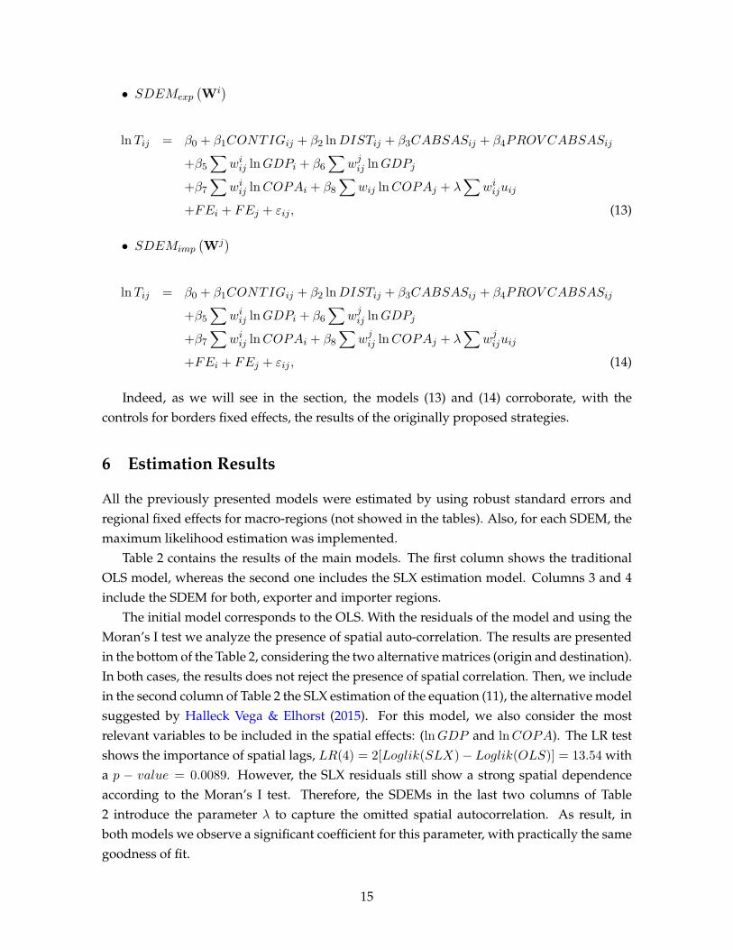
• SDEMexp(Wi

)

lnTij = β0 + β1CONTIGij + β2 lnDISTij + β3CABSASij + β4PROV CABSASij

+β5∑

wiij lnGDPi + β6∑

wjij lnGDPj+β7

∑wiij lnCOPAi + β8

∑wij lnCOPAj + λ

∑wiijuij

+FEi + FEj + εij , (13)

• SDEMimp(Wj

)

lnTij = β0 + β1CONTIGij + β2 lnDISTij + β3CABSASij + β4PROV CABSASij

+β5∑

wiij lnGDPi + β6∑

wjij lnGDPj+β7

∑wiij lnCOPAi + β8

∑wjij lnCOPAj + λ

∑wjijuij

+FEi + FEj + εij , (14)

Indeed, as we will see in the section, the models (13) and (14) corroborate, with thecontrols for borders fixed effects, the results of the originally proposed strategies.

6 Estimation Results

All the previously presented models were estimated by using robust standard errors andregional fixed effects for macro-regions (not showed in the tables). Also, for each SDEM, themaximum likelihood estimation was implemented.

Table 2 contains the results of the main models. The first column shows the traditionalOLS model, whereas the second one includes the SLX estimation model. Columns 3 and 4include the SDEM for both, exporter and importer regions.

The initial model corresponds to the OLS. With the residuals of the model and using theMoran’s I test we analyze the presence of spatial auto-correlation. The results are presentedin the bottom of the Table 2, considering the two alternative matrices (origin and destination).In both cases, the results does not reject the presence of spatial correlation. Then, we includein the second column of Table 2 the SLX estimation of the equation (11), the alternative modelsuggested by Halleck Vega & Elhorst (2015). For this model, we also consider the mostrelevant variables to be included in the spatial effects: (lnGDP and lnCOPA). The LR testshows the importance of spatial lags, LR(4) = 2[Loglik(SLX) − Loglik(OLS)] = 13.54 witha p − value = 0.0089. However, the SLX residuals still show a strong spatial dependenceaccording to the Moran’s I test. Therefore, the SDEMs in the last two columns of Table2 introduce the parameter λ to capture the omitted spatial autocorrelation. As result, inboth models we observe a significant coefficient for this parameter, with practically the samegoodness of fit.

15

It is interesting to note that, the variables corresponding to the baseline gravityspecification (lnGDPi, lnGDPj , CONTIGij , lnDISTij) are highly significant in all modelsand display coefficients with the expected signs. The income elasticity of bilateral trade is notsignificantly different to unity in origin and destination provinces, but it seems to be higherin the latter case, showing a higher relative effect from the attracting market. In the case ofthe population, a proxy variable of local market dynamic, the results are similar, but for thespatially adjusted models, the origin population elasticity is higher than the destination one.

The distance coefficient is −0.82 for the OLS model, and this value is very close tothe number obtained for the spatial models, which means that the inclusion of spatialinformation does not generate any important correction for the geographical distance. Thedistance coefficient is also in line with the international results, McCallum (1995) founds adistance coefficient ranging from −1.12 to −1.42, Anderson & Van Wincoop (2003) showvalues from −0.79 to −1.25, and Millimet & Osang (2007) found that in their basic modelthe elasticity with respect to distance is approximately one in absolute value. In the case ofBrazil, Daumal & Zignago (2010) found a larger distance coefficient of −1.82, in a model thatalso includes foreign trade by Brazilian states.

It should be noted that the contiguity effect is always positive and with an elasticity closeto one. Again, the effect is robust not only for the OLS but also in the case of the spatialmodels, where the coefficient is slightly reduced. As we shall see, in Table 3, the contiguityresult is supported by the borders effects model.

In general, the results of the canonical gravity model extended to consider origin anddestination hold and are coincidental with those observed in applications to the bilateraldomestic trade of other countries. This result is an interesting indication of the benefits ofthe database, which, as we indicated, is novel in Argentina.

After controlling the consistency of the basic model, we analyzed the impact on trade ofthe financial flows from the federal coparticipation arrangement, informality level, the useof different payments methods and the centrality effect of CABA and Buenos Aires.

First, as can be seen in Table 2, in the case of federal financial transfers, the coefficientsare significant and negative, both for origin lnCOPAi and destination lnCOPAj . Infact, the negative effect is significant for the origin rather than for the destination.8

Furthermore, when we introduce the neighborhood effects, we see that the origin, givenby

∑wiij lnCOPAi is significant with a negative effect closed to one. This means that an

increment of 1% of coparticipation for the neighboring provinces of origin region reducestrade flow in more than 1% in all models, all other things being equal (the impact is greaterfor spatial models).

Second, the lowest income at the provincial level, a proxy for the informality level, resultsin a negative effect over bilateral trade. The coefficient seems to be larger in the originprovince, but are significant and negative in both cases.

8For the destination province the effect is significant only for some specifications.

16

Table 2: Estimation of Alternative Models.

Models OLS SLX SDEM exp SDEM imp

lnGDPi 1.04∗∗∗ 0.93∗∗∗ 0.89∗∗∗ 0.99∗∗∗

(0.24)∗∗ (0.24)∗∗ (0.29)∗∗ (0.23)∗∗

lnGDPj 1.13∗∗∗ 1.20∗∗∗ 1.25∗∗∗ 1.19∗∗∗

(0.34)∗∗ (0.36)∗∗ (0.39)∗∗ (0.47)∗∗

CONTIGij 1.03∗∗∗ 1.00∗∗∗ 0.95∗∗∗ 0.97∗∗∗

(0.14)∗∗ (0.14)∗∗ (0.20)∗∗ (0.20)∗∗

lnDISTij −0.82∗∗∗ −0.83∗∗∗ −0.81∗∗∗ −0.81∗∗∗

(0.06)∗∗ (0.06)∗∗ (0.05)∗∗ (0.05)∗∗

lnPOPi 1.01∗∗∗ 1.51∗∗∗ 1.57∗∗∗ 1.33∗∗∗

(0.35)∗∗ (0.46)∗∗ (0.52)∗∗ (0.43)∗∗

lnPOPj 1.02∗∗∗ 1.20∗∗∗ 1.02∗∗∗ 1.20∗∗∗

(0.52)∗∗ (0.48)∗∗ (0.51)∗∗ (0.63)∗∗

lnCOPAi −1.19∗∗∗ −1.73∗∗∗ −1.71∗∗∗ −1.49∗∗∗

(0.49)∗∗ (0.60)∗∗ (0.65)∗∗ (0.52)∗∗

lnCOPAj −0.82∗∗∗ −1.38∗∗∗ −1.09∗∗∗ −1.27∗∗∗

(0.55)∗∗ (0.68)∗∗ (0.63)∗∗ (0.81)∗∗

Quintile12i −1.52∗∗∗ −2.04∗∗∗ −2.08∗∗∗ −1.84∗∗∗

(0.39)∗∗ (0.47)∗∗ (0.55)∗∗ (0.40)∗∗

Quintile12j −1.85∗∗∗ −1.85∗∗∗ −1.73∗∗∗ −1.89∗∗∗

(0.62)∗∗ (0.59)∗∗ (0.44)∗∗ (0.61)∗∗

GtoTotCashi 0.04∗∗∗ 0.06∗∗∗ 0.07∗∗∗ 0.06∗∗∗

(0.02)∗∗ (0.02)∗∗ (0.02)∗∗ (0.02)∗∗

GtoTotCashj 0.08∗∗∗ 0.08∗∗∗ 0.08∗∗∗ 0.09∗∗∗

(0.03)∗∗ (0.03)∗∗ (0.02)∗∗ (0.02)∗∗

GtoTotCredi 0.15∗∗∗ 0.17∗∗∗ 0.18∗∗∗ 0.18∗∗∗

(0.05)∗∗ (0.05)∗∗ (0.04)∗∗ (0.03)∗∗

GtoTotCredj 0.20∗∗∗ 0.20∗∗∗ 0.21∗∗∗ 0.21∗∗∗

(0.07)∗∗ (0.07)∗∗ (0.04)∗∗ (0.05)∗∗

CABSASij −4.46∗∗∗ −4.83∗∗∗ −5.05∗∗∗ −4.96∗∗∗

(0.65)∗∗ (1.31)∗∗ (1.52)∗∗ (1.49)∗∗

PROV CABSASij −0.27∗∗∗ −0.41∗∗∗ −0.61∗∗∗ −0.55∗∗∗

(0.18)∗∗ (0.50)∗∗ (0.60)∗∗ (0.58)∗∗

Wi × lnGDPi 0.47∗∗∗ 0.50∗∗∗ 0.46∗∗∗

(0.23)∗∗ (0.26)∗∗ (0.20)∗∗

Wj × lnGDPj 0.46∗∗∗ 0.48∗∗∗ 0.47∗∗∗

(0.35)∗∗ (0.33)∗∗ (0.38)∗∗

Wi × lnCOPAi −0.91∗∗∗ −0.90∗∗∗ −0.90∗∗∗

(0.29)∗∗ (0.34)∗∗ (0.25)∗∗

Wj × lnCOPAj −0.77∗∗∗ −0.72∗∗∗ −0.70∗∗∗

(0.55)∗∗ (0.46)∗∗ (0.56)∗∗

λ̂ 0.20∗∗∗ 0.20∗∗∗

(0.04)∗∗ (0.04)∗∗

Moran’s I (Wi) 0.19∗∗∗ 0.20∗∗∗

Moran’s I (Wj ) 0.22∗∗∗ 0.20∗∗∗

AIC 2325.97∗∗∗ 2320.43∗∗∗ 2301.16∗∗∗ 2300.81∗∗∗

Loglik −1141.99∗∗∗ −1135.22∗∗∗ −1123.58∗∗∗ −1123.41∗∗∗

Note: Constant term omitted. Robust SE in brackets. Regional Fixed effects included. ∗ p < 0.10, ∗∗ p < 0.05, ∗∗∗ p < 0.01.

Third, in the case of payments methods, the results indicate a positive correlation withbilateral trade, that is more important and significant in the case of credit payments methods.Traditionally, the sales achieved by the turnover tax (both final and intermediate) involvetransactions along the production chain that are, in many cases, financed by using creditboth formal and informal. This effect is captured in the empirical model where the creditvariable shows a positive and significant effect.

Fourth, the border effect of CABA and Buenos Aires (CABSASij) discourages theinterprovincial trade. In all models the coefficient is negative and significant, indicating thatthe centralism of CABA and Buenos Aires has, overall, a negative and significant impacton bilateral provincial trade. These results indicate a relative trade bias associated with thestrong relative importance of CABA and Buenos Aires both in production and market size.It is interesting to note that this centralism, already observed in historical times, continues tohave an influence on bilateral trade between the provinces.

As proposed by Feenstra (2002) we include the estimations with exporter and importerfixed effects. The inclusion of these fixed effects allows capturing unobserved characteristicsof the regions. However, these inclusion excludes province-specific variables, such aslnGDP and lnCOPA of the exporter and importer regions. Hence, only bilateral and spatiallags can be included in the model. Table 3 indicates the results of the alternative models withborder effects. As mentioned before, the contiguity coefficient maintains its significance withan elasticity close to one. Whereas the distance parameter shows a negative and significantelasticity, coinciding with the parameters found in the previous specifications.

Figures 5 and 6 allow comparing the results of the two spatial specifications. In thefigures, the value of the coefficients is given by the central point and the length of thesegment indicates the significance (with a significance level of 5%). If the segment cut thezero line, indicates that the parameter is not significant for the econometric specificationunder analysis.

18

Table 3: Estimation of Alternative Models with Border Effects.

Models OLS SLX SDEM exp SDEM imp

CONTIGij 1.01∗∗∗ 0.90∗∗∗ 0.82∗∗∗ 0.84∗∗∗

(0.16)∗∗ (0.16)∗∗ (0.19)∗∗ (0.20)∗∗

lnDISTij −0.80∗∗∗ −0.77∗∗∗ −0.75∗∗∗ −0.75∗∗∗

(0.06)∗∗ (0.06)∗∗ (0.05)∗∗ (0.05)∗∗

Wi × lnGDPi 2.36∗∗∗ 2.40∗∗∗ 2.38∗∗∗

(0.32)∗∗ (0.52)∗∗ (0.37)∗∗

Wj × lnGDPj 1.09∗∗∗ −0.05∗∗∗ −0.03∗∗∗

(0.20)∗∗ (0.37)∗∗ (0.35)∗∗

Wi × lnCOPAi −2.07∗∗∗ −2.10∗∗∗ −2.09∗∗∗

(0.39)∗∗ (0.64)∗∗ (0.42)∗∗

Wj × lnCOPAj −1.45∗∗∗ −0.90∗∗∗ −0.91∗∗∗

(0.33)∗∗ (0.38)∗∗ (0.54)∗∗

λ̂ 0.22∗∗∗ 0.22∗∗∗

(0.04)∗∗ (0.04)∗∗

Moran’s I (Wi) 0.22∗∗∗ 0.22∗∗∗

Moran’s I (Wj ) 0.26∗∗∗ 0.22∗∗∗

AIC 2382.78∗∗∗ 2338.11∗∗∗ 2313.41∗∗∗ 2313.19∗∗∗

Loglik −1145.39∗∗∗ −1120.05∗∗∗ −1105.71∗∗∗ −1105.59∗∗∗

Note: Constant term omitted. Robust SE in brackets. Regional Fixed effects included. ∗ p < 0.10, ∗∗ p < 0.05, ∗∗∗ p < 0.01.

Figure 5 shows the direct effect of coparticipation, both for origin and destination. Inthe case of origin, all the coefficients are significant for all the econometric specifications.However, the direct effect for the destination is only significant for the SLX model. Theindirect effects are significant for the origin, but not significant for the destination province.This result indicates that the indirect effect derived from the co-participation received bythe neighboring provinces of origin has a negative impact on bilateral trade. However, theindirect effect derived from the neighborhood of the destination province is not significant.

Figure 6 includes the coefficients corresponding to the indirect coparticipation effects forthe model with border effects (Table 3), when the fixed effects of origin and destination areconsidered. The graphs show that the indirect impact of the origin neighborhood remainssignificant. On the other hand, the indirect impact of the destination neighborhood is onlysignificant for SLX be model and SDEM be (imp).

19

Figure 5: Regression coefficients from alternative models (at 95% CI).

Figure 6: Comparison regression coefficients: basic and with border effects (at 95% CI).

20

7 Conclusions and Next Steps

This paper explores the standard gravity model for Argentina with a novel database oftrade finding similar results to the literature. This a factor that emphasizes the relevance ofsystematizing the processing of this database to generate a proxy for bilateral trade betweenthe provinces.

It should be noted that income distribution, measured as the two lowest quintiles in theprovince reduces bilateral trade. Also, formal payments have effect in bilateral trade. Cashand especially credit card payments have a positive effect, reflecting differences related tothe type of expenditures and/or the fiscal implications of using different formal paymentsmethods as well as the relevance of credit in commercial transactions.

We control for several socioeconomic variables and the results are consistent and robust.Our spatial models are robust using different spatial weighing matrices, W’s, and the spatiallocal effects of GDP are positive on trade in origin, but these spatial effects are negative forcoparticipation.

These last results indicate that national transfers from the redistribution federalarrangement are an important determinant of the inter-provincial trade generating negativespillover effects between the provinces. Indeed, the coparticipation as a redistributionmechanism of income towards lagging provinces discourages the inter-provincial tradeflows (significant in the origin but not in the destination). This negative impact is reinforcedby the coparticipation received by the provinces located in the vicinity of the origin province.

This home bias effect may be related to several factors, including the presence oftax surcharges on extraterritorial goods and services as well as provincial professionalenrollment regulations and local public procurement incentives. These factors may end upenhancing the consumption of locally produced goods and services and discouraging theirexport to other provinces.

Next steps in our agenda include different extensions. On one hand, we pretend toexplore competitive models in spatial econometrics, including new advances in estimationtechniques. On the other hand, we will explore the border and interaction effectsof CABA/Buenos Aires and the rest of the provinces, including the economic sectorsdesegregation and the effect of provincial foreign trade.

References

Álvarez, I. C., Barbero, J., Rodríguez-Pose, A., & Zofío, J. L. (2018). Does institutionalquality matter for trade? institutional conditions in a sectoral trade framework. WorldDevelopment, 103, 72–87.

Anderson, J. E. & Van Wincoop, E. (2003). Gravity with gravitas: A solution to the borderpuzzle. American economic review, 93(1), 170–192.

21

Anselin, L. (1988). Spatial econometrics: Methods and models, volume 4. Springer Netherlands.

Anselin, L. (2002). Under the hood issues in the specification and interpretation of spatialregression models. Agricultural Economics, 27(3), 247–267.

Arias, R. (2011). Ensayos sobre la teoría de la evasión y la elusión de impuestos indirectos. PhDthesis, Universidad Nacional de la Plata.

Asiain, A. (2014). Alejandro bunge (1880-1943: Un conservador defensor de la independenciaeconómica y la soberanía nacional. Ciclos en la historia, la economía y la sociedad, 22(43), 6.

Blanco, E., Elosegui, P., Izaguirre, A., & Montes-Rojas, G. (2019). Regional and stateheterogeneity of monetary shocks in argentina. The Journal of Economic Asymmetries, 20,e00129.

Bunge, A. E. (1940). Una nueva argentina. G. Kraft ltda.

Caliendo, L., Parro, F., Rossi-Hansberg, E., & Sarte, P.-D. (2018). The impact of regional andsectoral productivity changes on the us economy. The Review of economic studies, 85(4),2042–2096.

Colina, J. (2019). Estimación de la competitividad de las provincias argentinas en base a sus balancesde comercio intra-nacional. Technical report, Informe 1, IDESA.

Combes, P.-P., Lafourcade, M., & Mayer, T. (2005). The trade-creating effects of business andsocial networks: evidence from france. Journal of international Economics, 66(1), 1–29.

Daumal, M. & Zignago, S. (2010). Measure and determinants of border effects of brazilianstates. Papers in Regional Science, 89(4), 735–758.

Elhorst, J. P. (2014). Spatial Econometrics. From Cross-sectional data to Spatial Panels.SpringerBriefs in Regional Science, Springer.

Elosegui, P. & Pinto, S. (2018). Comercio interprovincial en argentina: Una aproximaciónbasada en la información del convenio multilateral del impuesto a los ingresos brutos.Blog BCRA, Central Bank of Argentina.

Elosegui, P., Sangiacomo, M., & Pinto, S. (2021). Towards a cash less economy: the case ofargentina. Working Paper BCRA.

Fally, T., Paillacar, R., & Terra, C. (2010). Economic geography and wages in brazil: Evidencefrom micro-data. Journal of Development Economics, 91(1), 155–168.

Feenstra, R. (2002). Border effects and the gravity equation: Consistent methods forestimation. Scottish Journal of Political Economy, 49(5), 491–506.

22

Fischer, M. & Griffith, D. (2008). Modeling spatial autocorrelation in spatial interaction data:an application to patent citation data in the european union. Journal of Regional Science,48(5), 969–989.

Halleck Vega, S. & Elhorst, J. P. (2015). The slx model. Journal of Regional Science, 55(3),339–363.

Head, K. & Mayer, T. (2010). Illusory border effects: Distance mismeasurement inflatesestimates of home bias in trade. In P. van Bergeijk & S. Brakman (Eds.), The gravitymodel in international trade: Advances and applications chapter 6, (pp. 165 – 192). CambridgeUniversity Press.

LeSage, J. & Pace, R. (2009). Introduction to spatial econometrics. CRC press.

LeSage, J. & Pace, R. K. (2008). Spatial econometric modeling of origin-destination flows.Journal of Regional Science, 48(5), 941–967.

McCallum, J. (1995). National borders matter: Canada-us regional trade patterns. TheAmerican Economic Review, 85(3), 615–623.

Millimet, D. & Osang, T. (2007). Do state borders matter for u.s. intranational trade? therole of history and internal migration. Canadian Journal of Economics/Revue canadienned’économique, 40(1), 93–126.

Moran, P. A. (1950). Notes on continuous stochastic phenomena. Biometrika, (pp. 17–23).

Poncet, S. (2005). A fragmented china: Measure and determinants of chinese domesticmarket disintegration. Review of international Economics, 13(3), 409–430.

Porto, A. (2018). Transferencias intergubernamentales y disparidades fiscales a nivel subnacional enArgentina. Technical report, Documento para discusión No IDB-DP-494, BID.

Porto, A. & Elizagaray, A. (2011). Regional development, regional disparities and publicpolicies in argentina: a long-run view. In The Economies of Argentina and Brazil. EdwardElgar Publishing.

Requena, F. & Llano, C. (2010). The border effects in spain: an industry-level analysis.Empirica, 37(4), 455–476.

Sen, A. & Smith, T. (1995). Gravity models of spatial interaction behavior. Springer, Heidelberg.

Tinbergen, J. (1962). Shaping the world economy; suggestions for an international economic policy.Twentieth Century Fund.

Tombe, T. & Winter, J. (2021). Fiscal integration with internal trade: Quantifying the effectsof federal transfers in canada. Canadian Journal of Economics/Revue canadienne d’économique.

23

Wei, S.-J. (1996). Intra-national versus international trade: how stubborn are nations in globalintegration? Technical report, National Bureau of Economic Research.

Yilmazkuday, H. (2012). Understanding interstate trade patterns. Journal of InternationalEconomics, 86(1), 158–166.

24

Appendix

Table A: Provinces, size of GDP and population (%).

Name Acronym Region G.D.P. % POP. %

Buenos Aires BsAs Pampean 35.09 38.64Autonomous City of Buenos Aires CABA Pampean 18.57 6.96Santa Fe StaFe Pampean 9.78 7.84Córdoba CBA Pampean 8.32 8.28Mendoza MZA Cuyo 4.00 4.38Neuquén NEU Patagonic 2.70 1.45Entre Ríos ER Pampean 2.49 3.06Chubut CHU Patagonic 2.13 1.33Tucumán TUC Northwest 1.66 3.71Salta SAL Northwest 1.61 3.11San Luis SL Cuyo 1.41 1.11Santa Cruz StaCr Patagonic 1.40 0.77Río Negro RN Patagonic 1.23 1.63Chaco CHA Northeast 1.18 2.65Misiones MIS Northeast 1.16 2.77Santiago del Estero SdE Northwest 1.00 2.15San Juan SJ Cuyo 0.99 1.72Corrientes CORR Northeast 0.96 2.48Tierra del Fuego TdF Patagonic 0.85 0.36La Pampa LP Patagonic 0.84 0.79Jujuy JUJ Northwest 0.78 1.69Catamarca CAT Northwest 0.74 0.92La Rioja LR Northwest 0.67 0.86Formosa FOR Northeast 0.46 1.34

Table B shows the information of the matrix used in the paper, Wmix = Wcontd2, and thealternative weighting matrix used in Tables D and E.

Table B: Information of spatial weighting matrices.Elements Wcont W4nn Wcontd2 W4nnd2

Minimum weight > 0 0.167 0.250 0.0004319 0.0008657Mean weight 0.428 0.250 0.0017361 0.0017361

Non zero weights (%) 0.667 0.696 0.667 0.696Mean neighbors 3.83 4

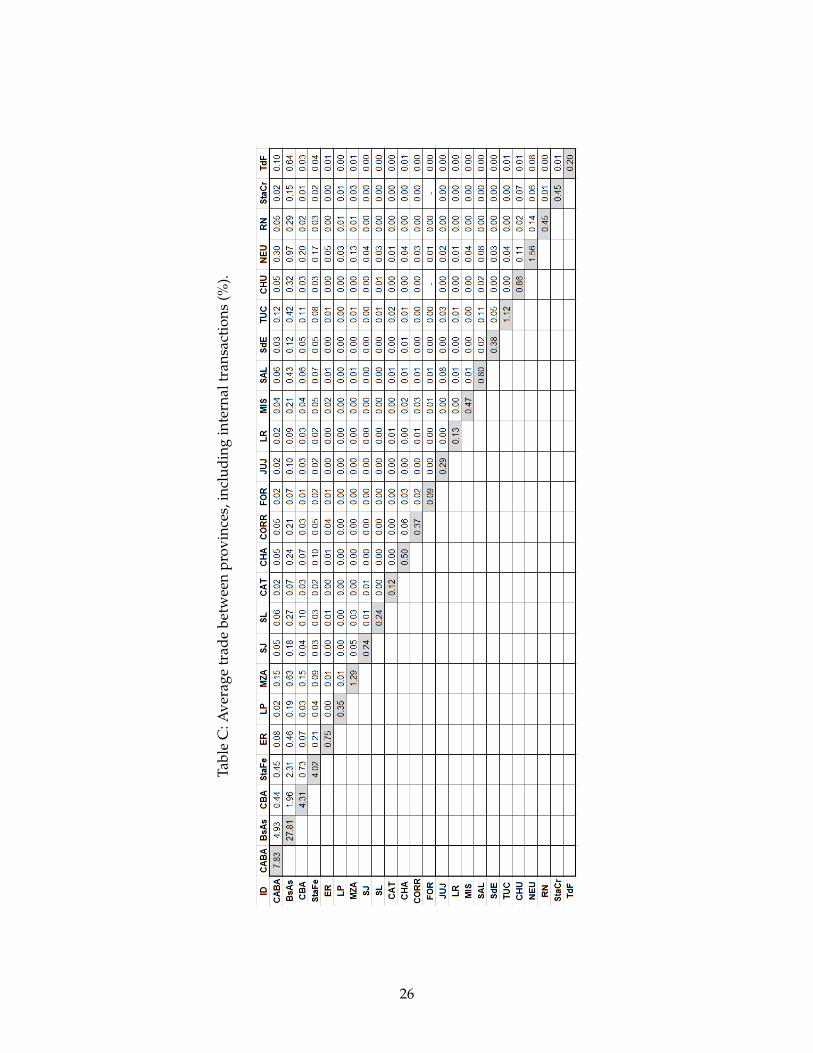
Tabl

eC

:Ave

rage

trad

ebe

twee

npr

ovin

ces,

incl

udin

gin

tern

altr

ansa

ctio

ns(%

).

26

Table D: Estimation of Alternative Models under Wmix = W4nnd2.

Models OLS SLX SDEM exp SDEM imp

lnGDPi 1.04∗∗∗ 0.95∗∗∗ 0.94∗∗∗ 0.96∗∗∗

(0.24)∗∗ (0.26)∗∗ (0.29)∗∗ (0.24)∗∗

lnGDPj 1.13∗∗∗ 1.14∗∗∗ 1.12∗∗∗ 1.13∗∗∗

(0.34)∗∗ (0.34)∗∗ (0.38)∗∗ (0.45)∗∗

CONTIGij 1.03∗∗∗ 0.99∗∗∗ 0.94∗∗∗ 0.95∗∗∗

(0.14)∗∗ (0.14)∗∗ (0.20)∗∗ (0.20)∗∗

lnDISTij −0.82∗∗∗ −0.83∗∗∗ −0.80∗∗∗ −0.80∗∗∗

(0.06)∗∗ (0.06)∗∗ (0.05)∗∗ (0.05)∗∗

lnPOPi 1.01∗∗∗ 1.47∗∗∗ 1.49∗∗∗ 1.42∗∗∗

(0.35)∗∗ (0.44)∗∗ (0.51)∗∗ (0.43)∗∗

lnPOPj 1.02∗∗∗ 1.21∗∗∗ 1.20∗∗∗ 1.20∗∗∗

(0.52)∗∗ (0.49)∗∗ (0.50)∗∗ (0.62)∗∗

lnCOPAi −1.19∗∗∗ −1.71∗∗∗ −1.69∗∗∗ −1.62∗∗∗

(0.49)∗∗ (0.57)∗∗ (0.65)∗∗ (0.52)∗∗

lnCOPAj −0.82∗∗∗ −1.35∗∗∗ −1.27∗∗∗ −1.24∗∗∗

(0.55)∗∗ (0.70)∗∗ (0.68)∗∗ (0.87)∗∗

Quintile12i −1.52∗∗∗ −2.04∗∗∗ −2.06∗∗∗ −1.92∗∗∗

(0.39)∗∗ (0.44)∗∗ (0.55)∗∗ (0.42)∗∗

Quintile12j −1.85∗∗∗ −1.89∗∗∗ −1.84∗∗∗ −1.91∗∗∗

(0.62)∗∗ (0.60)∗∗ (0.46)∗∗ (0.60)∗∗

GtoTotCashi 0.04∗∗∗ 0.07∗∗∗ 0.07∗∗∗ 0.07∗∗∗

(0.02)∗∗ (0.02)∗∗ (0.02)∗∗ (0.02)∗∗

GtoTotCashj 0.08∗∗∗ 0.08∗∗∗ 0.08∗∗∗ 0.08∗∗∗

(0.03)∗∗ (0.03)∗∗ (0.02)∗∗ (0.03)∗∗

GtoTotCredi 0.15∗∗∗ 0.17∗∗∗ 0.17∗∗∗ 0.18∗∗∗

(0.05)∗∗ (0.05)∗∗ (0.04)∗∗ (0.04)∗∗

GtoTotCredj 0.20∗∗∗ 0.20∗∗∗ 0.20∗∗∗ 0.20∗∗∗

(0.07)∗∗ (0.07)∗∗ (0.04)∗∗ (0.05)∗∗

CABSASij −4.46∗∗∗ −4.49∗∗∗ −4.52∗∗∗ −4.48∗∗∗

(0.65)∗∗ (1.10)∗∗ (1.45)∗∗ (1.44)∗∗

PROV CABSASij −0.27∗∗∗ −0.25∗∗∗ −0.35∗∗∗ −0.32∗∗∗

(0.18)∗∗ (0.39)∗∗ (0.56)∗∗ (0.55)∗∗

Wi × lnGDPi 0.40∗∗∗ 0.41∗∗∗ 0.39∗∗∗

(0.17)∗∗ (0.26)∗∗ (0.20)∗∗

Wj × lnGDPj 0.34∗∗∗ 0.35∗∗∗ 0.32∗∗∗

(0.27)∗∗ (0.35)∗∗ (0.42)∗∗

Wi × lnCOPAi −0.86∗∗∗ −0.85∗∗∗ −0.85∗∗∗

(0.21)∗∗ (0.33)∗∗ (0.25)∗∗

Wj × lnCOPAj −0.65∗∗∗ −0.63∗∗∗ −0.55∗∗∗

(0.51)∗∗ (0.56)∗∗ (0.69)∗∗

λ̂ 0.17∗∗∗ 0.18∗∗∗

(0.04)∗∗ (0.04)∗∗

Moran’s I (Wi) 0.17∗∗∗ 0.18∗∗∗

Moran’s I (Wj ) 0.19∗∗∗ 0.17∗∗∗

AIC 2325.97∗∗∗ 2322.80∗∗∗ 2309.08∗∗∗ 2308.54∗∗∗

BIC 2417.45∗∗∗ 2431.70∗∗∗ 2426.69∗∗∗ 2426.16∗∗∗

Note: Constant terms are omitted. Std. errors in parentheses. Fixed effects included. ∗ p < 0.10, ∗∗ p < 0.05, ∗∗∗ p < 0.01.

27

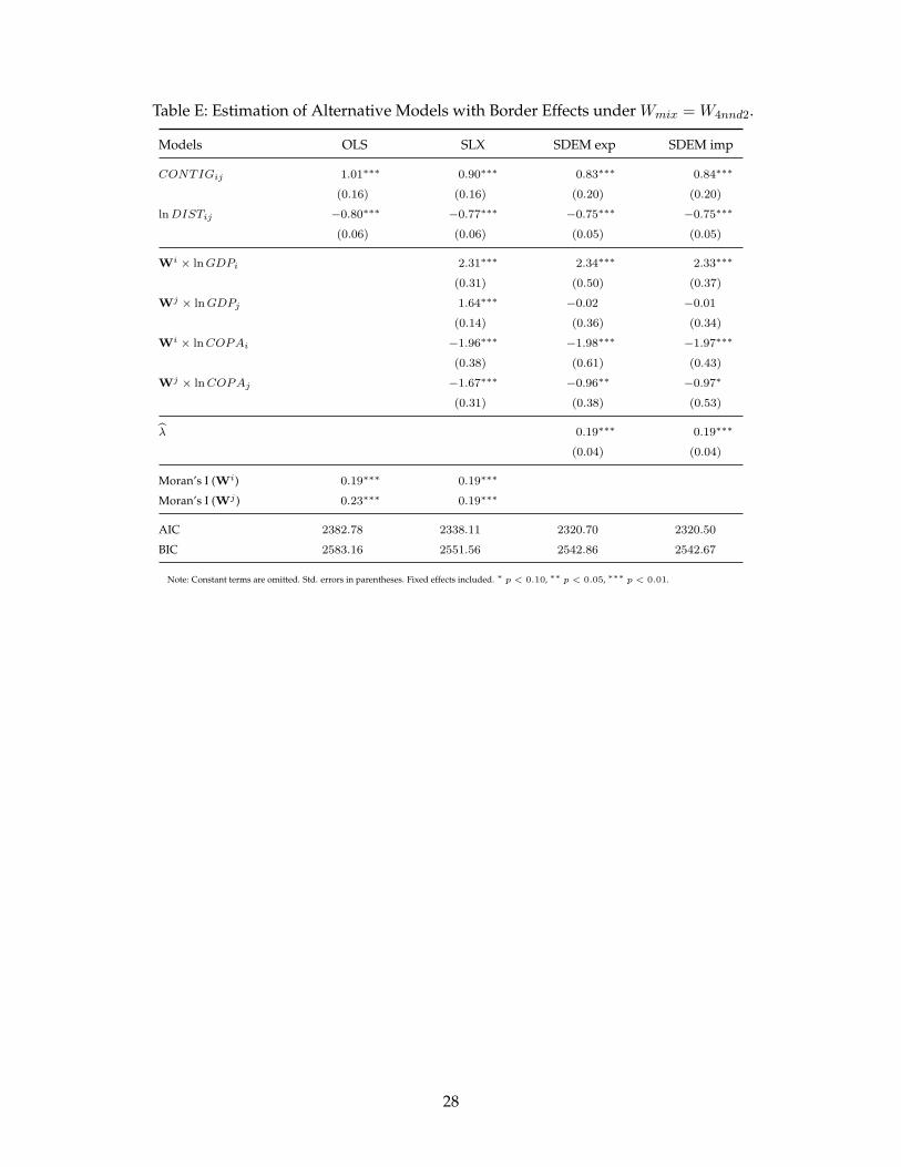
Table E: Estimation of Alternative Models with Border Effects under Wmix = W4nnd2.

Models OLS SLX SDEM exp SDEM imp

CONTIGij 1.01∗∗∗ 0.90∗∗∗ 0.83∗∗∗ 0.84∗∗∗

(0.16)∗∗ (0.16)∗∗ (0.20)∗∗ (0.20)∗∗

lnDISTij −0.80∗∗∗ −0.77∗∗∗ −0.75∗∗∗ −0.75∗∗∗

(0.06)∗∗ (0.06)∗∗ (0.05)∗∗ (0.05)∗∗

Wi × lnGDPi 2.31∗∗∗ 2.34∗∗∗ 2.33∗∗∗

(0.31)∗∗ (0.50)∗∗ (0.37)∗∗

Wj × lnGDPj 1.64∗∗∗ −0.02∗∗∗ −0.01∗∗∗

(0.14)∗∗ (0.36)∗∗ (0.34)∗∗

Wi × lnCOPAi −1.96∗∗∗ −1.98∗∗∗ −1.97∗∗∗

(0.38)∗∗ (0.61)∗∗ (0.43)∗∗

Wj × lnCOPAj −1.67∗∗∗ −0.96∗∗∗ −0.97∗∗∗

(0.31)∗∗ (0.38)∗∗ (0.53)∗∗

λ̂ 0.19∗∗∗ 0.19∗∗∗

(0.04)∗∗ (0.04)∗∗

Moran’s I (Wi) 0.19∗∗∗ 0.19∗∗∗

Moran’s I (Wj ) 0.23∗∗∗ 0.19∗∗∗

AIC 2382.78∗∗∗ 2338.11∗∗∗ 2320.70∗∗∗ 2320.50∗∗∗

BIC 2583.16∗∗∗ 2551.56∗∗∗ 2542.86∗∗∗ 2542.67∗∗∗

Note: Constant terms are omitted. Std. errors in parentheses. Fixed effects included. ∗ p < 0.10, ∗∗ p < 0.05, ∗∗∗ p < 0.01.

28