Working Paper 94-12 / Document de travail 94-12 · Working Paper 94-12 / Document de travail 94-12 ... ISSN 1192-5434 ISBN 0-662-22804-9 ... (NBR) are used in their analysis.5

Bank of Canada Banque du Canada

Working Paper 94-12 / Document de travail 94-12

Searching for the Liquidity Effectin Canada

byBen Fung and Rohit Gupta

December 1994

Searching for the Liquidity Effectin Canada

by

Ben S. C. Fung and Rohit Gupta

Department of Monetary and Financial Analysis

Bank of Canada

Ottawa, Ontario

Canada

K1A 0G9

Tel.: (613) 782-7582

Fax: (613) 782-7508

The views expressed here are those of the authors.

No responsibility for them should be attributed to the Bank of Canada.

Acknowledgments

An earlier version of this paper was presented at the Canadian Economics Association meetingsin Calgary, 10-13 June 1994. We would like to thank Kevin Clinton, Walter Engert andJack Selody for very helpful discussions and suggestions. The paper has also benefited fromcomments by Pierre Duguay, Chuck Freedman, Donna Howard, Dave Longworth and seminarparticipants at the Bank of Canada. We also thank the Securities Department of the Bank andespecially Glen Snow for compiling the data on excess cash reserves. Jamie Armour providedadditional research assistance for the current version of this paper. Of course, all errors are ourown.

ISSN 1192-5434

ISBN 0-662-22804-9

Printed in Canada on recycled paper

Contents

Abstract/ Résumé......................................................................................................................... v

1 Introduction .......................................................................................................................... 1

2 A review of the empirical work on liquidity effects............................................................. 4

3 Methodology: structural vector autoregression and identification ....................................... 7

4 Empirical results .................................................................................................................. 104.1 The data...................................................................................................................... 10

4.1.1 Liquidity measures............................................................................................ 104.1.2 Rates and macro-variables ................................................................................ 11

4.2 The dynamic responses.............................................................................................. 124.2.1 Impulse response functions............................................................................... 124.2.2 Variance decompositions .................................................................................. 15

4.3 Sensitivity analysis .................................................................................................... 164.3.1 Sample period sensitivity tests.......................................................................... 164.3.2 Sensitivity with respect to different measures of interest rates......................... 174.3.3 Summary........................................................................................................... 17

5 Concluding remarks.............................................................................................................. 19

Appendix 1: Description of the data ............................................................................................ 21

Appendix 2: Identification of the structural VAR ....................................................................... 23

Tables .......................................................................................................................................... 27

Graphs and figures ....................................................................................................................... 31

Bibliography................................................................................................................................. 49

iii

Abstract

This paper examines the empirical evidence of the liquidity effect in Canada. In the presence of the

liquidity effect, the initial impact of an unanticipated expansionary monetary policy is to lower

nominal and real interest rates for a short period of time. Eventually, however, the anticipated

inflation effect will come into force and dominate the liquidity effect as people adjust their inflation

expectations to the new money growth rate. As a result, interest rates will then increase. In this

paper, we use vector autoregression (VAR) methods to study how interest rates, output and

exchange rates respond to shocks to monetary policy. We use the excess cash reserves of the

chartered banks and the surprise component of excess cash reserves as measures of monetary

policy shocks. Shocks to monetary policy are measured by the orthogonalized innovations to these

liquidity variables. We find that expansionary shocks to monetary policy are followed by declines

in the interest rate, increases in output, and depreciations of the Canadian dollar. The results are

robust to different orderings of the variables used in the VAR estimation. The response of the

interest rate to monetary policy shocks is robust to different measures of liquidity, but the responses

of other variables vary slightly.

Résumé

Les auteurs examinent empiriquement la pertinence des effets de liquidité au Canada. Sous

l’hypothèse d’effet de liquidité, l’incidence initiale d’un choc expansionniste non anticipé de la

politique monétaire consiste en une diminution momentanée des taux d’intérêt nominaux et réels.

Cependant, comme les anticipations d’inflation s’ajustent au nouveau taux d’expansion monétaire,

leur effet finit par se manifester et dominer l’effet de liquidité. Les taux d’intérêt se mettent alors à

augmenter. Dans leur étude, les auteurs font appel à la méthode d’estimation des vecteurs

autorégressifs pour étudier comment les taux d’intérêt, la production et les taux de change

réagissent aux chocs de politique monétaire. Ils se servent des réserves excédentaires des banques

à charte et de leur composante non anticipée comme mesures des chocs de la politique monétaire.

Plus précisément, ceux-ci sont mesurés par les innovations orthogonalisées de ces variables de

liquidité. Les auteurs ont observé que les chocs expansionnistes de politique monétaire sont suivis

par des baisses de taux d’intérêt, des hausses de la production et des dépréciations du dollar

canadien. Les résultats obtenus résistent bien aux changements d’agencement des variables

utilisées dans l’estimation des vecteurs autorégressifs. La réaction des taux d’intérêt aux chocs de

politique monétaire est peu sensible aux diverses mesures de liquidité utilisées, mais la réaction des

autres variables a tendance à varier légèrement.

v

1

1 Introduction

The purpose of this paper is to examine the empirical evidence of the liquidity effect in Canada. In

particular, we investigate how strong and persistent the liquidity effect is. In the presence of such

an effect, the initial impact of an unanticipated expansionary monetary policy is to lower nominal

and real interest rates for a short period of time. Eventually, however, the anticipated inflation effect

will come into force and dominate the liquidity effect as people adjust their inflation expectations

to the new money growth rate. As a result, interest rates will then increase. The strength of the

liquidity effect can be measured by the size of the negative response of interest rates to

expansionary policy, and its persistence can be measured by the length of time before interest rates

start to rise.

According to the prevailing view, the Bank of Canada influences very short-term interest

rates, such as the call loan rate, by varying the supply of settlement balances. The level of the call

loan rate is targeted with a view towards achieving a particular level of monetary conditions,

expressed as a linear combination of the 90-day interest rate and the trade-weighted exchange

rate. The movements in interest rates and the exchange rate then affect consumer spending,

investment and net exports, resulting in a change in aggregate demand and output (an open-

economy IS curve relationship). The level of aggregate demand relative to aggregate supply puts

pressure on the inflation rate through a Phillips curve relationship.1 Our paper will focus on the

empirical evidence of the effect of policy-induced shocks to the supply of settlement balances on

the call loan rate.

Recently, there has been a surge of interest and significant progress in the study of the

liquidity effect. Empirical studies by Christiano and Eichenbaum (1992a) and Strongin (1992)

find strong evidence supporting the presence of liquidity effects in the United States. General

equilibrium models by Lucas (1990), Furest (1992), and Christiano and Eichenbaum (1992b),

developed along the lines of Grossman and Weiss (1983) and Rotemberg (1984), have been

successful in generating a strong and persistent liquidity effect. These models consist of four

different agents: the household, the firm, the monetary authority and the financial intermediary,

and they rely on the heterogeneous impacts of monetary policy to generate the liquidity effect.

One attractive feature of these models is that money and financial intermediaries play very

important roles: money is required by firms to finance production and by consumers to purchase

consumption goods, and any monetary injections are transmitted to the economy through

1. This is a highly simplified description of the current Bank of Canada view. For a detailed review, see Crow (1988)and Duguay (1994).

2

financial intermediaries. The key assumption is that households cannot continuously revise their

consumption and savings decisions.2 Thus, after a money shock, for example a monetary

expansion, households cannot immediately adjust the quantity of cash spent on consumption to

the changed financial market circumstances. The intermediaries, which have become more liquid

because of the newly injected cash, have to lower the interest rate to encourage firms to borrow

more. As a result, investment and business activities are stimulated and production is increased.

As incomes rise, households will also adjust their consumption and savings decisions, and the

price level will eventually adjust to the new money growth rate.

Liquidity-effect models are interesting because they provide a view of the transmission

mechanism in which money and financial intermediaries play important roles. As the Bank of

Canada injects settlement balances into the payments system, the direct-clearing financial

institutions – in particular, the major chartered banks – become more liquid because of the cash

injection. Since deposits at the Bank of Canada pay no interest, the banks attempt to dispose of the

extra cash by lending it to investment dealers in the special call loan market, thus increasing their

holdings of earning liquid assets and putting downward pressure on the call loan rate. Moreover,

the banks may desire to increase their holdings of less liquid assets by making loans more

available and at a lower rate, especially when they perceive the cash injections as an easy

monetary policy. The additional liquidity stimulates borrowing, thus increasing investment and

economic activity. As employment and wages increase, households revise their consumption-

savings decisions. Eventually, the price level will adjust to the increase in liquidity and the system

will move back to an equilibrium.

In this paper, we use vector autoregression (VAR) methods to study how interest rates,

output and exchange rates respond to shocks to monetary policy. Several studies in the liquidity-

effect literature argue that inference about the effects of monetary policy on interest rates depends

critically on the identification assumptions adopted to measure the exogenous component of

changes in monetary policy and on the measure of liquidity used. The most widely used measures

of monetary policy shocks, such as innovations to conventional monetary aggregates, are

inconsistent with the actual operating procedures of the Bank of Canada or the Federal Reserve.

Moreover, Christiano and Eichenbaum (1992a) and Strongin (1992) report that in the United

States the use of these types of measures, for example, M1, leads to misleading inferences.

2. Christiano, Eichenbaum and Evans (1994) study the flows-of-funds data in the United States and find that net fundsraised by the household sector remain unchanged for several quarters after a monetary shock. This finding isconsistent with the assumption that households do not adjust their consumption-savings decisions immediately after amonetary shock.

3

Therefore, in this paper, we use the excess cash reserves of the chartered banks and the surprise

component of excess cash as measures of monetary policy shocks.3 Shocks to monetary policy

are measured by the orthogonalized innovations to these liquidity variables.

The major findings of the paper can be summarized as follows. We find that when excess

cash is used as a measure of liquidity, expansionary shocks to monetary policy are followed by

declines in the interest rate, increases in output, and depreciations of the Canadian dollar. The

results are robust to different orderings of the variables used in the VAR estimation. The response

of the interest rate to monetary policy shocks is robust to different measures of liquidity, but the

responses of other variables vary slightly. The evidence on the liquidity effect is strongest when

excess cash is employed as the measure of liquidity. This result is consistent with the view that the

Bank of Canada implements its policy by controlling the supply of excess cash to the financial

system. Our findings are in line with similar studies in the United States. However, liquidity

effects in Canada are relatively short-lived compared to the empirical results reported in

Christiano and Eichenbaum (1992a) and Strongin (1992), lasting for about three to six months.

When the non-borrowed reserve mix (NBRX) is used as the liquidity measure over the period

1959:1 to 1992:2, Strongin finds that a one-standard deviation shock inNBRX causes the federal

funds rate to decline for almost seven months.4 Christiano and Eichenbaum find that the liquidity

effect lasts for almost four years when non-borrowed reserves (NBR) are used in their analysis.5

The relatively short-lived liquidity effect in Canada may be due to the fact that, over the sample

period 1977 to 1991, people had built up highly sensitive inflationary expectations so that the

liquidity effect was quickly dominated by the anticipated inflation effect a few months after the

money supply shock. Moreover, the sample period that we use in this study is short compared to

the studies by Strongin and Christiano and Eichenbaum.

The remainder of the paper is organized as follows. Section 2 briefly reviews the empirical

work on liquidity effects. Section 3 describes the methodology and discusses the identification of

the structural VAR. Section 4 presents the empirical results. The final section offers some

concluding remarks.

3. Detailed descriptions of these cash reserve measures can be found in Section 4 and Appendix 1.

4. NBRX is the ratio of non-borrowed reserves to the lag of total reserves.

5. NBR is total reserves less total borrowings from the Federal Reserve by depository institutions.

4

2 A review of the empirical work on liquidity effects

There has been much debate about the empirical evidence of the liquidity effect. However, recent

empirical studies, most notably Christiano and Eichenbaum (1992a) and Strongin (1992), argue

that there is strong evidence of the presence of liquidity effects in the United States. These studies

suggest that NBR is the best measure of money in the United States and that the liquidity effect is

a significant and persistent feature of the U.S. economy. In this section, we briefly review some of

the empirical studies on liquidity effects in the United States. These studies also motivate our

present work to study the empirical evidence of the liquidity effect in Canada.

Many of the early empirical studies do not find evidence of the liquidity effect. Most of the

earlier econometric studies identify positive innovations in monetary aggregates or negative

innovations in the short-term interest rates as expansionary money supply shocks. The traditional

approach to measuring the liquidity effect, used in Cagan and Gandolfi (1969), Melvin (1983) and

Cochrane (1989), is to regress the interest rate on current and past money growth.

Cagan and Gandolfi (1969) study the relationship between the commercial paper rate and

M2 for the period 1910-65. They find that the paper rate reaches a trough six months after an

increase in money growth. The positive impact of money on interest rates occurs only after a

considerable lag. Melvin (1983) extends the analysis to include M2 data drawn from the 1970s.

He finds that the liquidity effect is much shorter-lived over the 1973-79 period. The initial

liquidity effect of faster money growth is likely to be offset within the month following the

monetary policy change. Melvin dubs the finding “the vanishing liquidity effect” and attributes it

to enhanced inflation sensitivity that causes the anticipated inflation effect of a monetary

expansion to dominate the liquidity effect. High inflation rates in the 1970s may account for the

reduction in the duration of the liquidity effect from that experienced in earlier decades. Cochrane

(1989) subsequently finds that the liquidity effect reemerges during the 1979-82 period when the

Federal Reserve targeted non-borrowed reserves, lasting at least a few months.6

The empirical evidence presented in these earlier studies, which are based on the

traditional approach, suggests that the relationship between innovations in money aggregates and

interest rates varies over time and is not as persistent in some periods as the liquidity hypothesis

would suggest.

6. The data used are the Monday auction average 3-month treasury bill rate and non-seasonally adjustedM1.

5

Leeper and Gordon (1992) point out that the distributed lag regressions implicitly assume

that no other variables induce interest rates and money growth to move together to generate the

correlations estimated in the traditional approach. To explore this possibility, they estimate a four-

variable VAR that includes money growth, interest rates, consumer prices and industrial

production. They study the relationship between monthly series of the monetary base and the

federal funds rate over the 1954-90 period. They identify innovations in the monetary base

(instead of M2, for example) as exogenous policy disturbances by arguing that the monetary base

is the Federal Reserve’s control variable and is more closely associated with the open market

operations that underlie the liquidity effect. Two versions of the VAR are estimated, one in which

money growth is exogenous and one that is completely unrestricted. The correlation between

unanticipated monetary growth and the funds rate is never negative and is strongly positive in

some subperiods.

Recent empirical studies of the liquidity effect by Christiano and Eichenbaum (1992a) and

Strongin (1992) argue that the use of broad money aggregates such as M1 or M2 is inappropriate.

These aggregates are largely influenced by the shocks in the demand for money and are not

directly related to the Federal Reserve’s policy action.

Christiano and Eichenbaum argue that NBR is the appropriate measure of money in

studying the liquidity effect. The level of NBR is directly controlled by the Federal Open Market

Committee through open market operations. Therefore, it is a suitable measure of money to use in

identifying and estimating the effects of monetary policy shocks. Christiano and Eichenbaum

perform VARs on monthly and quarterly data that include a measure of money, the federal funds

rate, a measure of aggregate real output and the price level.

The dynamic response of the federal funds rate to a shock in monetary policy is studied

using different measures of money, namely M0, M1 and NBR. When NBR is used in the analysis,

the federal funds rate displays a sharp, large, persistent decline in response to expansionary

policy, regardless of which identifying assumptions are used, regardless of which postwar sample

period is used and regardless of whether monthly or quarterly data are used. Unanticipated

expansionary policy shocks always drive down short-term interest rates and increase real output.

Strongin argues that in actual practice the Federal Reserve accommodates innovations in

the demand for reserves, and he suggests that policy innovations can be identified as those

changes in the mix of borrowed reserves and NBR that are not the result of the Federal Reserve’s

accommodation of demand innovations. Strongin’s study considers monthly data from 1959:1 to

1992:2 and subsamples similar to those in Leeper and Gordon. Two sets of VARs are presented

6

for each subsample. The first set is a three-variable VAR containing total reserves (TR), the non-

borrowed reserve mix (NBRX) and the federal funds rate (FF). The second set includes two more

variables: the log of industrial production and the log of the consumer price index. He finds that

for the entire period and for each subsample, there is a clear liquidity effect. It is always negative

and highly significant.

The empirical studies for the United States show that it is important to choose an

appropriate measure of money – likely NBR – for studying the liquidity effect. These studies also

show that it is necessary to properly identify monetary policy shocks. In Canada, the framework

for implementing monetary policy is very different from that in the United States, and there is no

direct empirical counterpart to the NBR used for the measure of money in the United States.

Therefore we focus our study on using excess cash as a measure of liquidity. The level of excess

cash is directly influenced by the Bank of Canada through the cash setting, which in turn,

influences the call loan rate. We believe that excess cash is a suitable measure of liquidity to

identify and estimate the effects of monetary policy shocks. We will discuss our liquidity

measures in more detail in Section 4.

7

3 Methodology: structural vector autoregression and identification

The approach used in the present study is the structural vector autoregression (SVAR) approach

employed by Bernanke (1986), Sims (1986, 1992), and Christiano and Eichenbaum (1992a). This

technique allows us to use economic theory to transform the reduced-form VAR model into a

system of structural equations. The SVAR yields impulse responses and variance decompositions

that can be given structural interpretations. We begin this section with a brief description of the

SVAR approach.

Suppose the economy evolves according to

. (1)

HereXt is a vector of variables summarizing the state of the economic system. In this study, we

consider a six-variable VAR consisting of a measure of liquidity (M), interest rate (R), output (Y),

the price level (P), exchange rate (PFX) and the U.S. federal funds rate (FF). The matrixA is a

square matrix of structural parameters on the contemporaneous endogenous variables that

indicates the contemporaneous relationships in the model.C(L) is a matrix polynomial in positive

powers of the lag operatorL. The structural disturbances in this economy are summarized by the

identically, independently distributed random variableεt, which is a vector of white noise.

Equation (1) can be transformed into the following reduced form:

, (2)

whereβ(L) = A-1C(L) andet = A-1εt. This is a VAR representation of the structural model in (1).

The SVAR approach that we employ here imposes restrictions onA and the covariance

matrix of the structural shocks(Σε), which are both 6 by 6 matrices, to identify these structural

parameters from the covariance matrix of the residuals (Σe).7 Specifically,Σε is specified as a

diagonal matrix, because the primitive structural disturbances are assumed to originate from

independent sources andΣε is further normalized to be the identity matrix.8 However, additional

restrictions are still required to identify the matrixA. The type of restriction most relevant for the

7. This is commonly called the contemporaneous approach. For more details about SVAR and different identificationapproaches, see Keating (1992) and Watson (1993).

8. This is similar to the normalization restrictions used in Chamie, DeSerres and Lalonde (1994). As shown inAppendix 2, an alternative way of normalization is to set the main diagonal elements ofA to unity because eachstructural equation is normalized on a particular endogenous variable. Both ways impose additionaln restrictions(n=6 here).

AXt C L( ) Xt 1− εt+=

Xt β L( ) Xt 1− et+=

8

existing liquidity literature is to put restrictions on the contemporaneous nature of feedback

between the elements ofXt. One common way is to adopt a particular Wold causal interpretation

of the data. The idea is to assume that the matrixA is lower triangular when the variables inXt are

ordered according to their causal priority.

When the variables inXt are ordered as {M, R, Y, P, PFX, FF}, they indicate that

unanticipated changes in monetary policy are measured by the innovations inM. This view

corresponds to the assumption that the contemporaneous portion of the Bank of Canada’s

feedback rule for settingMt does not involveRt, Yt or other contemporaneous variables. The Wold

ordering of {FF, M, R, Y, P, PFX} implies that the unanticipated change in monetary policy is

measured by the portion of the innovation inMt that is orthogonal to the innovation inFFt. This

outlook corresponds to the assumption that the contemporaneous portion of the central bank’s

feedback rule for settingMt involvesFFt, but notRt, Yt or other contemporaneous variables.

The different identification schemes that we consider in this study are summarized in

Table 1 (p. 27). The orderings that we use are very similar to those used by Christiano and

Eichenbaum (1992), Eichenbaum and Evans (1993), Sims (1992) and Strongin (1992). This

similarity facilitates comparison of our findings with U.S. studies.

There are basically two sets of orderings: one withFF appearing first and one withFF

appearing last in the Wold causal chain. We consider the ordering in which the federal funds rate

is first in the causal chain to be more reasonable, since the Canadian variables have little influence

on the federal funds rate. However, this ordering also assumes that the Bank of Canada may take

the federal funds rate into consideration when settingMt. Alternatively, we consider ordering the

federal funds rate last in the causal chain. In this case, we assume that the Bank’s feedback rule

for settingMt does not involve the federal funds rate.

Among all the orderings, we consider those in whichFF and PFXappear first and Yand P

appear last to be the most appropriate. The assumption that the contemporaneous portion of the

Bank of Canada’s feedback rule for setting monetary policy involvesFFt and PFXt (or Rt, if Rt

appears beforeMt in the ordering) is consistent with the view that the Bank of Canada reacts to

current financial conditions. Besides, current month values on economic variables such asY andP

would not be available until at least one month later. The results to be reported in Section 4,

however, show that the empirical findings are robust to the different orderings used in the study.

The estimation of the SVAR proceeds as follows. First, the reduced form VAR represented

in equation (2), with adequate lags of each variable, is estimated by ordinary least squares (OLS).

Second, the structural parameters inA and the structural disturbances are identified. Standard

9

errors of the impulse response and variance decomposition functions are then calculated using a

Monte Carlo simulation in order to construct their confidence bands.9

9. The Monte Carlo procedure employed here is the normal approximation procedure outlined in Doan (1990).

10

4 Empirical results

4.1 The data

This section examines the dynamic responses of the variables of interest to monetary policy

shocks. In deciding which variables to include in our study, we have to face the following trade-

off. In order to minimize omitted-variable bias, we would like to include as many relevant variables

in our VAR system as possible. However, the set of variables must be limited, as each equation has

many lags of each variable. Should the variable set become too large, the model would exhaust the

available data. Therefore, the variable set chosen includes the following domestic variables: a

measure of liquidity, the interest rate, output and the price level. Given the openness of the

Canadian economy, we also include the Canada-U.S. nominal exchange rate and the U.S. federal

funds rate. Appendix 1 provides a detailed description of the data used. The data are monthly. A

six-variable VAR for each ordering is estimated in levels (except output and the consumer price

index, which are in log-levels).10 Six lags of each variable are included in the VARs along with a

constant term.11

4.1.1 Liquidity measures

We consider both excess cash and cash surprise as measures of liquidity. Excess cash reserves are

chartered bank deposits at the Bank of Canada in excess of the statutory minimum. Essentially,

excess cash is a measure of the supply of liquidity to the banking system. We also take excess cash

to be the target policy setting of the Bank of Canada. Data on excess cash is available on a daily

basis from 1977:8. In order to get the monthly observations on excess cash, that is, the total

cumulative net cash positions of the chartered banks over a month, we consider two alternative

10. Unit-root tests indicate that all variables are integrated of order one or two, except for the liquidity measurevariables, which are stationary. However, Sims, Stock and Watson (1990) argue that the common practice oftransforming models to stationary form is unnecessary in many cases. Specifically, in “large enough” samples, theOLS estimator is consistent whether or not the VAR (in levels) contains integrated components (p. 113). Impulseresponse analysis relies on consistent parameter estimates. This requirement is satisfied when a VAR is estimated inlevels. Similar estimations on levels were used in Christiano and Eichenbaum (1992a), Sims (1992), and Strongin(1992).

11. The Akaike Information Criterion for VAR optimal lag selection as outlined in Judge et al. (1988) gives anoptimal lag length of 2 for the VAR systems. We chose to use a lag of 6 in order to capture more dynamics in thesystem, as monetary policy is presumed to affect the economy with a lag, as well as to be consistent with otherstudies. The results for the impulse response and variance decomposition functions when using a lag of 2 arequalitatively the same as those presented. However, the fluctuations are smoother and the magnitude of changes is, insome cases, different. Eichenbaum and Evans (1993) and Strongin (1992) also chose 6 lags for their analysis. Giventhat our sample runs from 1977:8 to 1991:10, which is slightly more than 14 years of monthly observations, there areless than two complete business cycles in this period. Therefore, in order to capture the monetary policy content ofthis period, a half-year lag seems appropriate.

11

methods of cumulating the data: first, by calculating the average of the two end-of-period

cumulative excess cash positions (EC1), and second, by taking the average of the two mid-period

cumulative excess cash positions (EC2).12 Cash surprise (CS) is the cumulative total of the

differences between thetarget policy setting of excess cash supplied by the Bank of Canada and

the amount of excess cashexpected by the chartered banks.13 It indicates the extent to which the

Bank intends to surprise the banking system in its reserve provision, and hence measures the

Bank’s desire to put pressure in one direction or the other on the short-term interest rate. Graph 1a

(p. 31) depictsEC1 andEC2 together, while Graph 1b (p. 31) plotsCS.

WhenEC1 or EC2 is used as a measure of liquidity, the regressions are run over 1977:8–

1991:10. We begin our estimation from 1977, as the mid-period cumulative excess cash

position (EC2) is available only from 1977:8. Starting in November 1991, the Bank of Canada

changed its system of implementing monetary policy in anticipation of the phasing-out of reserve

requirements that began in mid-1992. The calculation period became a month. In addition, the

Bank of Canada started to target the settlement balances of all direct clearers in the Canadian

Payments Association (CPA) rather than those of the chartered banks alone.14 Therefore, we

chose to end the estimation in 1991:10 in order to maintain the consistency of the cash

management system over the sample period. We consider only monthly data because of the

relatively short sample period. When cash surprise is used as the liquidity measure, the

regressions are run over 1987:1–1991:10, because data on the chartered banks’ expectations of

cash setting begin in 1987. In this system, only three lags are included due to the small sample

size.

4.1.2 Rates and macro-variables

The relevant short-term interest rates are the call loan rate (Rcall), the 90-day commercial paper

rate (R90), and the 90-day treasury bill rate (RTB90). Graphs 2a and 2b (p. 32) plotRcall and the

Rcall - R90 spread respectively. The other relevant variables that are considered in this study are

12. Donna Howard of the Bank of Canada has pointed out that the monetary policy content may be netted out if wecumulate excess cash through each calculation period. For instance, there have been averaging periods when thebanks have had large negative excess reserves in the first half of an averaging period, but by the close of theaveraging period they have had a large positive excess reserve as the Bank provided more cash to the system in thelatter half. Therefore, we also cumulate the excess reserves to the middle of each averaging period.

13. The Bank of Canada obtains the cash targets of the direct clearers each day by direct communication; see Clintonand Howard (1994).

14. Direct clearing members of the CPA include the Bank of Canada, the six major banks and seven other large banksand non-bank deposit-taking institutions. All other institutions have clearing and settlement accounts with the directclearers.

12

output measured by industrial production (Y), the consumer price index (P), the nominal Canada-

U.S. exchange rate (PFX), and the U.S. federal funds rate (FF). The interest rates and the exchange

rate used are the averages of the daily observations over a month, exceptfor RTB90, which is the

end-of-month observation.

4.2 The dynamic responses

4.2.1 Impulse response functions

The impulse response function (IRF) results are reported in Figures 1 through 12 (pp. 33-44). The

Wold orderings used in the estimations are given in the title of the figures. These results display the

response of each variable in the system to a one-standard deviation shock in the liquidity variable.

The columns correspond to each of the three liquidity measures employed in the study:EC1, EC2,

andCS respectively. For example, the third row of the first column in Figure 1 (p. 33) shows the

dynamic response ofRcall to a one-standard deviation shock inEC1. We are most interested in the

effects of an unanticipated monetary policy shock onRcall, Y andPFX. The solid lines in the

figures represent the impulse response functions, while the dashed lines correspond to the 95 per

cent upper and lower confidence bands about the point estimate of the IRF.15 A response can be

thought to be significant if both bands, as well as the point estimate, lie on the same side of the zero

line. (The units for the call loan rate and the federal funds rate are in percentages, so that 0.5 on the

scale indicates 50 basis points, for example, and the units for the liquidity measures are in millions

of dollars.)

We begin by considering the results of the VAR under a Wold causal ordering of {FF, M,

R, Y, P, PFX}. This ordering corresponds to the assumption that thecontemporaneous portion of

the Bank of Canada’s feedback rule for setting monetary policy involvesFFt but notRt, Yt, Pt or

PFXt.16Thus, a monetary policy shock is measured by the component of the innovation inMt that

is orthogonal to the innovation inFFt. These results are presented in Figure 1. Responses are

shown over a horizon of 48 months.

Consider first the findings whenEC1 is employed as the monetary policy variable.

Following positive innovations to monetary policy,Rcall declines significantly and stays below

its preshock level for about three months. The effects of the monetary policy shock on Rcall

15. The two standard deviation bands were computed using Monte Carlo simulations employing 1 000 randomdraws. The reported impulse response function is the average of the 1 000 Monte Carlo draws.

16. Note that no restrictions are imposed on the lagged components of the Bank of Canada’s feedback rule.

13

become insignificant after two months. The maximum impact of a one-standard deviation shock

(approximately $450 million) inEC1 onRcall equals 15 basis points and occurs within two

months of the monetary policy shock. Industrial production rises in the period after the shock and

stays above its preshock level for over a year. The effects on industrial production are significant

in the third month following the liquidity shocks. Another variable of interest is the exchange rate.

The response ofPFX to the liquidity shock is presented in the last row. Following the monetary

policy shock, the Canadian dollar depreciates slightly for about three months. However, the

effects on the exchange rate are not significant. Eichenbaum and Evans (1993) also find a

depreciation of the U.S. dollar after a positive liquidity shock. Their findings, though, are more

significant and stable. The response of the price level to a positive liquidity shock is initially

negative – but the negative response is weak and eventually becomes positive. This initial

counterintuitive response of the price level can also be found in Sims (1992) and Strongin (1992).

This “price puzzle” raises some difficulties for interpreting innovations in excess cash reserves as

monetary policy shocks. These are considered further below.

The results forEC2 are reported in the second column of Figure 1 and are quite similar to

those ofEC1 except that the effects are now more persistent. Following the monetary policy

shock,Rcall is below its preshock level for about six months, industrial production increases for

almost four years, and the Canadian dollar depreciates against the U.S. dollar for close to two

years. The maximum impact onRcall equals 20 basis points and occurs immediately after the

monetary policy shock. The effects of the monetary policy shocks onRcall andY are significant

for only about three months, however, while the effects onPFX are not significant. The response

of the price level is again counterintuitive. Prices drop significantly for about three months and

remain below the preshock level for over 48 months.

The results forCS, reported in column 3 in Figure 1, are mixed. Following the monetary

policy shock,Rcall is below its preshock level for about nine months with a significant effect for

one month. The maximum impact of a one-standard deviation shock (roughly $900 million) toCS

onRcall equals 8 basis points and occurs immediately after the monetary policy shock. Following

the monetary policy shock, there is a temporary increase in industrial production, immediately

followed by a decline. However, industrial production remains above its preshock level for over

four years, although the effect is not significant. The response of the exchange rate is rather

unstable but insignificant. This may be due to the relatively short sample period. Immediately

after impact, prices drop significantly for two months and remain below the preshock level for

over 48 months.

14

To sum up the results in Figure 1: regardless of which liquidity measure is used in the

analysis, a positive liquidity shock leads to a decline inRcall and an increase in output. The

statistical significance of the movements inRcall and output depends on the liquidity measures

used. In all cases, however, the declines inRcall are significant for at least the first two months

after impact. The increase in output is significant in the third month after impact when eitherEC1

or EC2 is used.

For all three measures of liquidity, the response of the price level poses some problems.

The price level drops after the positive liquidity shock and only eventually rises above the

preshock level whenEC1 is used. This price puzzle is also reported in Sims (1992) and Strongin

(1992). Sims studies the effects of monetary policies in five countries, including France,

Germany, Japan, the United States and the United Kingdom. When innovations in the interest rate

are used as a measure of monetary policy innovations, all five countries display some perverse

price effects initially. The positive responses of prices to positive innovations in the interest rate

are strong and persistent only in France and Japan. In the other countries, the responses are

weaker and eventually become negative. Strongin also reports the perverse price effect: following

a positive innovation inNBRX, the price level drops significantly for about eight months and only

rises above the preshock level after about 30 months.

Sims suggests that the perverse price effect may reflect the fact that the monetary authority

has some indicator of inflation in its reaction function that is missing from the VAR underlying

the monetary policy shock measures. Therefore, he includes a measure of commodity prices in the

VAR as a proxy for inflationary pressure and finds that the price responses are somewhat

improved. Christiano, Eichenbaum and Evans (1994) find that by including commodity prices in

the VAR, the responses of prices are no longer anomalous when either innovations in the federal

funds rate or NBR is used as a measure of monetary policy shocks.

In results not reported here, we find no perverse price effect when innovations inRcall are

used to measure monetary policy shocks. Following a positive shock inRcall, the price level

drops and always remains below the preshock level, although the response is not statistically

significant. However, as shown above, the price response is counterintuitive when excess cash

reserves are used. Unlike Christiano, Eichenbaum and Evans (1994), we have been unable to

resolve the price puzzle in our study by including either the commodity price index or the terms-

of-trade index.17

17. The commodity price index used is the Bank of Canada commodity price index. The terms-of-trade index used isthe ratio of the price of Canadian commodities to the price of U.S. manufactured goods.

15

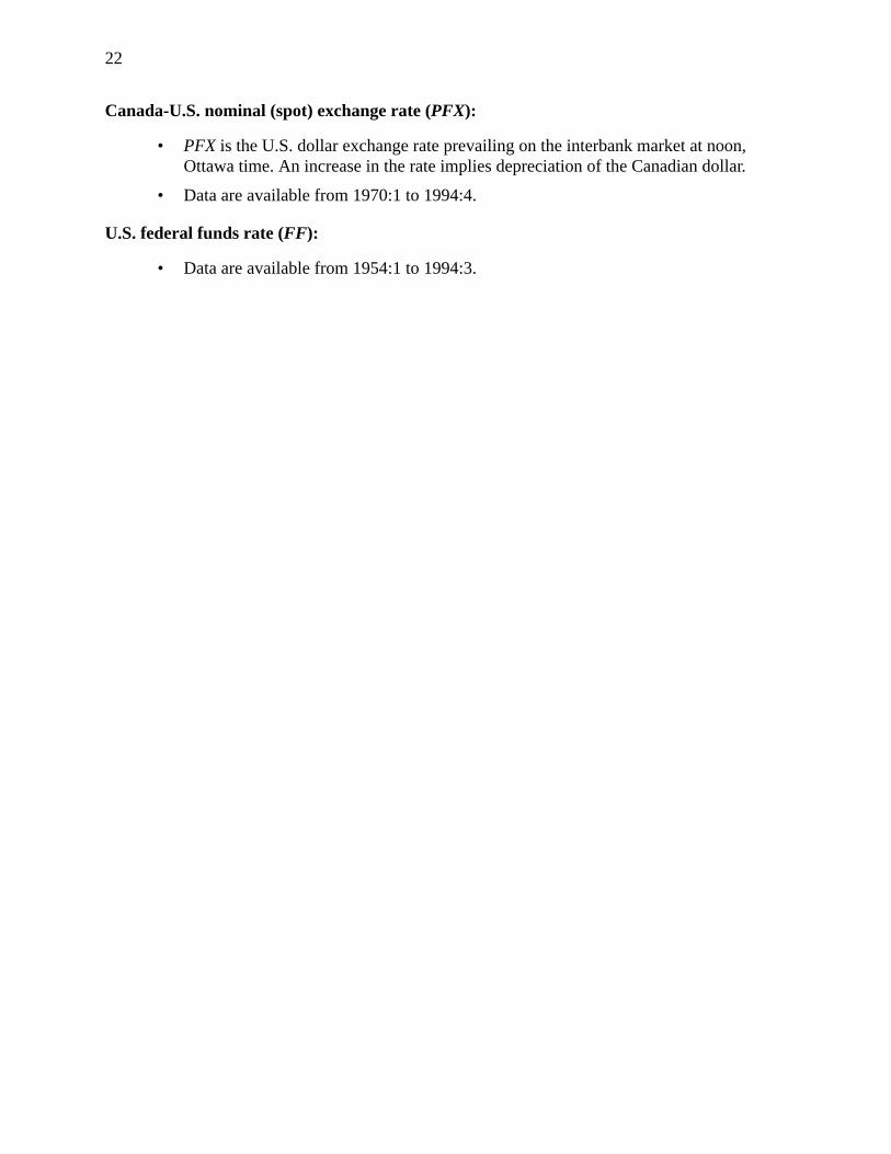
The results of the VAR reported above are robust to different Wold orderings. The results

for the remaining 11 orderings are shown in Figures 2 to 12 (pp. 34-44). For all measures of

liquidity used in this study, unanticipated expansionary monetary shocks lead to significant

declines in the call loan rates and significant increases in output, regardless of the ordering used in

the VAR. However, the persistence of such effects varies among different measures of liquidity.

The declines in the call loan rate range from three months whenEC1 is used as the measure of

liquidity to about one year whenCS is used. Output increases for about 15 months whenEC1 is

used as the measure of liquidity and increases over the 48-month horizon whenEC2 is used.

WhenCS is used, the response of output is rather unstable and sensitive to the orderings. The

statistical significance of these responses depends on the ordering of the VAR estimation. For all

orderings, the declines inRcall are rarely significant after three months whenEC1 or EC2 is used

and are not significant after six months whenCS is used. For all orderings, the increases in output

are not significant after three months whenEC1 or EC2 is used, and the responses of output are

never significant whenCS is used.

These findings are consistent with similar studies in the United States and support the

presence of liquidity effects in Canada. An unanticipated expansionary monetary policy lowers

the interest rate, stimulates output and leads to a depreciation of the Canadian dollar. These results

are consistent with the operation of monetary policy by the Bank of Canada and support the view

that the Bank of Canada can influence the call loan rate by affecting the level of excess cash

reserves of the chartered banks.

4.2.2 Variance decompositions

Finally, we briefly turn to the overall contribution of monetary policy shocks to the variability of

other variables. We compute the percentage of the variance of the j-step ahead forecast error of

each variable that is attributable to monetary policy shocks. Tables 3 through 5 (pp. 28-29) report

the variance decomposition functions (VDF) of each measure of liquidity over different horizons

for the ordering of {FF, M, R, Y, P, PFX} with the 95 per cent confidence bands about the VDF

point estimates.18 A significant effect is judged by a non-zero lower 95 per cent confidence band.

The estimated percentages forEC1 orEC2 are not very high and are not significant. About 1.9 per

cent (after 1 month) to 6.6 per cent (after 48 months) of variance inRcall can be explained by

innovations inEC1. The percentages of explained variance by innovations inEC2 are slightly

higher. For example, about 4.5 per cent to 8.4 per cent of the forecast error ofRcall can be

18. The confidence bands were computed using Monte Carlo simulations employing 1 000 random draws. Thereported variance decomposition function is the average of the 1 000 Monte Carlo draws.

16

explained by innovations inEC2. The VDFs forCS are reported in Table 5 (p. 29) and the

estimated percentages are higher than those forEC1 or EC2. About 11.4 per cent of the forecast

error variance ofYcan be accounted for significantly by innovations inCS, whereas 11.7 per cent

of the forecast error variance inPFXcan be explained by the innovations inCS, with the results

also being significant for over a year. The VDFs for each measure of liquidity are similar for

different orderings of the VAR estimation, except forCS. Therefore, we report only the VDFs for

one additional ordering of {FF, Y, P, M, R,PFX} in Tables 6 through 8 (pp. 29-30). As can be seen

in Table 8, about 19 to 24 per cent of the forecast error variance ofRcallcan be explained by the

innovations inCS,and the results are significant for over two years. Similar results can be found

in orderings (4), (10) and (12) from Table 1 (p. 27) (results are not reported in the paper). Despite

the insignificant variance decomposition functions, the impulse response functions forRcall andY

are significant from three to six months for all measures of liquidity.

4.3 Sensitivity analysis

In this subsection, we reexamine the VAR results in the previous subsection using different sample

periods and different measures of interest rates.

4.3.1 Sample period sensitivity tests

Here we examine the dynamic responses of the variables of interest to a liquidity shock over

different sample periods. SinceEC1 is available from 1971:6, we reestimate the VAR model with

the ordering {FF, M, R, Y, P, PFX} over the period 1971:6 to 1991:10. The dynamic responses of

Rcall, Y andPFX to a one-standard deviation shock inEC1 are graphed in Figure 13 (p. 45) and

are very similar to those reported in Figure 1. The output effect, however, has become marginally

insignificant.

We also examine this VAR system over the period 1971:6 to 1994:1, and the impulse

response functions are graphed in Figure 13 (p. 45). A liquidity shock causesRcall to decline for

about three months but the effect is now insignificant. Industrial production rises after the

liquidity shock and stays above its preshock level for over two years. The effects, however, are

not significant. The results are different from the estimations that include data only up to 1991:10.

We also extend the sample period forCS to 1994:1 and reexamine the model’s dynamic

responses. Following a liquidity shock,Rcall declines for about nine months but the effect is not

significant, and output increases for almost a year but the effect is only significant for about two

months. As explained in subsection 4.1.1 (p. 10), there was a change in the system of

implementation of monetary policy in November 1991. The results reported here suggest that the

17

change in procedure has lessened the ability of the VAR to detect liquidity effects over the full

sample period 1971 to 1994.

4.3.2 Sensitivity with respect to different measures of interest rates

The VAR estimations are also repeated using different measures of interest rates, namely, the

3-month treasury bill rate (RTB90) and the 3-month commercial paper rate (R90), instead ofRcall.

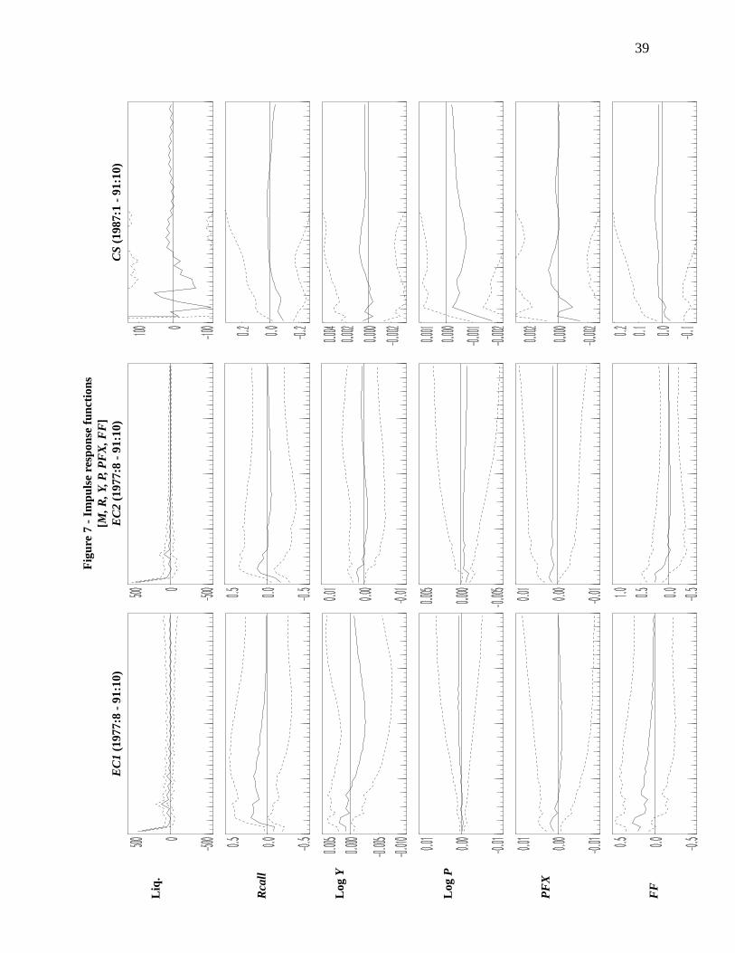
The impulse response functions for the ordering of {FF, M, R, Y, P, PFX} with RTB90 andR90 are

reported in Figures 14 and 15 (pp. 46-47) respectively.

WhenRTB90 is used, the dynamic responses of the variables in the VAR become more

sensitive to the Wold causal ordering for all three liquidity measures. We can still find some

significant negative interest rate responses to a liquidity shock. However, for some orderings, the

responses ofRTB90 are positive in the period after a positive liquidity shock.RTB90 stays above

the preshock level for a few months but the effects are insignificant. For all three liquidity

measures, the output effect of a positive liquidity shock is positive but is not significant.

Following a positive innovation inEC1 or EC2, output rises for about four months to a year. The

output effects of a positive shock inCS are very similar to the case whereRcall is used as the

interest rate; that is, the effects are positive for almost four years. The dynamic responses ofPFX

andP are not too sensitive to the use ofRTB90 as the interest rate, except that for most Wold

orderings the immediate response ofPFX to a liquidity shock is an appreciation in the Canadian

dollar. Again, this effect is not significant.

The IRFs for the VAR withR90 are very similar to those withRTB90. However, when

EC1 orEC2 is used as the liquidity measure,R90 rises immediately after the shock and the effects

are significant for some orderings. The positive interest rate effects are hardly significant beyond

two months after impact. The output effect of a shock inEC2 is positive and significant within

about three months of impact.

4.3.3 Summary

The main results in our study seem to be robust to different sample periods, although the change in

the monetary policy implementation procedures in 1991 and 1992 seem to have lessened the ability

of the VAR to detect liquidity effects over 1971 to 1994. The results, however, are more sensitive

to the uses of different interest rates. WhenRcall is used, the findings support the presence of

liquidity effects in Canada. In comparison withRTB90 or R90, the evidence of liquidity effects

becomes less obvious and depends on the ordering of the VAR estimation. This is consistent with

the view that the Bank of Canada has a large influence onRcall through the cash setting but has

18

only an indirect influence onRTB90 andR90; bothRTB90 andR90 are mainly determined by

money market conditions.

19

5 Concluding remarks

In this paper, we have studied the effects of a liquidity shock on the interest rate, output and the

exchange rate. The measures of liquidity that we have used in the study are the excess cash reserves

of the chartered banks. Since the Bank of Canada has direct control of excess cash through its daily

cash setting, it is a suitable measure of the Bank’s monetary policy actions. The major findings of

our study can be summarized as follows: we find that expansionary shocks to monetary policy are

followed by declines in the interest rates, an increase in output, and a depreciation of the Canadian

dollar. The results are robust to different orderings of the variables used in the VAR estimation. The

responses of interest rates to monetary policy shocks are robust to different measures of liquidity,

but the responses of other variables vary slightly.

The present study provides empirical evidence of liquidity effects in Canada. Looking

ahead, we believe it would be worthwhile to extend the present analysis by employing different

identification restrictions. Instead of restricting the contemporaneous matrix (A) to be lower

triangular, one could impose more realistic restrictions onA. For example, one can restrictA by

using the fact that monetary policy reacts to the monetary conditions index, thus specifying the

contemporaneous response ofM to a linear combination ofR andPFX. This kind of modification

may provide better identification of monetary policy shocks. Finally, it would be of interest and of

importance to construct a liquidity-effect model that reflects the Canadian institutional context

and in which both money and credit play important roles in the transmission of monetary policy.

Ultimately, such a model might be able to provide a useful theoretical framework for thinking

about monetary policy in Canada.

21

Appendix 1: Description of the data

Here the data used in the study are outlined. All the data are of a monthly frequency, except where

noted (for example, excess cash). The interest rates and the exchange rate are the averages of daily

observations over a month, except forRTB90, which is the end-of-month observation.

Money (M):

• Excess cash (EC) – Excess cash reserves are chartered bank deposits at the Bank ofCanada in excess of the statutory minimum. The monthly series is constructed fromdaily excess cash by cumulating the daily data over each averaging period. Twoalternative methods of cumulating the data are considered: first, by calculating theaverage of the two end-of-period cumulative excess cash positions (EC1), and second,by taking theaverage of the two mid-period cumulative excess cash positions (EC2).The end-of-period cumulation data is available from 1970:1 to 1994:3, while the mid-period data are available from 1977:8 to 1994:3.

• Cash surprise (CS) – Cash surprise is the difference between the target policy settingof excess cash reserves in the chartered banks and the setting that the chartered banksexpect to have attained as a result of their money market operations. The monthlyseries is constructed by cumulating the daily cash surprise over the averaging period.This series is available from 1987:1 to 1993:12.

Interest rates (R):

• Call loan rate (Rcall) – Special call loans are loans made to money market dealers fora short period of time to finance their inventory of money market securities. They werefirst introduced by the chartered banks in 1967 and subsequently became the mostimportant source of dealer financing from the chartered banks. Both reduced systemliquidity (a tight policy) and the building of inventory by dealers will put upwardpressure on the call loan rate. The series is available in the CANSIM data base from1975. However, daily high and lowRcall is available in the data base at the Bank ofCanada from June 1971. An average of the daily high and low call loan rates fromJune 1971 to December 1974 can be added toRcall to extend the series backwards.ThusRcall is available from 1971:6 to 1994:4.

• 90-day treasury bill rate (RTB90) – available from 1935.

• 90-day commercial paper rate (R90) – available from 1956.

Output (Y):

• Industrial production – Data in constant 1986 dollars are available on a monthly basisfrom 1961:1 to 1994:1.

Prices (P):

• CPI – available from 1914:1 to 1994:3.

22

Canada-U.S. nominal (spot) exchange rate (PFX):

• PFX is the U.S. dollar exchange rate prevailing on the interbank market at noon,Ottawa time. An increase in the rate implies depreciation of the Canadian dollar.

• Data are available from 1970:1 to 1994:4.

U.S. federal funds rate (FF ):

• Data are available from 1954:1 to 1994:3.

23

Appendix 2: Identification of the structural VAR

This appendix describes the identification of the structural VAR under the contemporaneous

approach similar to the one used in Christiano and Eichenbaum (1992a). The notation used is the

same as that used in Section 3.

Suppose the economy evolves according to

. (A2.1)

It can be transformed into the following reduced form:

, (A2.2)

whereβ(L) = A-1C(L) andet = A-1εt. Thus the covariance matrix for the reduced-form residualset

is related to that of the structural shocksεt in the following relation:

. (A2.3)

By estimating the reduced-form VAR in (A2.2) by OLS, we can obtain estimates for the

β’s andΣe, which hasn(n+1)/2 unique elements. However, we need to knowA first in order to

identify the structural shocksε from the reduced-form residualse. It can easily be seen from

(A2.3) that we need additional restrictions to recover bothA andΣε. This can be achieved by

imposingtheoretical restrictions to reduce the number of unknown structural parameters inA to

be less than or equal to the number of estimated parameters of the covariance matrix of the VAR

residuals.

Thecontemporaneous approach imposes restrictions on these two matrices: the

coefficient matrixA with n2 elements and the symmetric structural covariance matrixΣε with

n(n+1)/2 unique elements.1 At leastn2 restrictions have to be imposed onA andΣε to get the

structural models identified. First,Σε is specified as a diagonal matrix, because the primitive

structural disturbances are assumed to originate from independent sources, thus imposing

n(n-1)/2 restrictions. Second,n restrictions are imposed by normalization. This can be done in

two different ways. One way is to set the main diagonal elements ofA to unity as each structural

equation is normalized on a particular endogenous variable. As one endogenous variable in each

structural equation is usually regarded as the dependent variable, its coefficient can be arbitrarily

1. An alternative structural VAR method, developed by Shapiro and Watson (1988) and Blanchard and Quah (1989),uses long-run restrictions to identify the economic structure from the reduced form. For our purposes, however, thecontemporaneous approach seems more relevant.

AXt C L( ) Xt 1− εt+=

Xt β L( ) Xt 1− et+=

Σe E ete′t[ ] A 1− E εtε′t[ ] A′ 1− A 1− ΣεA′ 1−= = =

24

set at unity. Alternatively, we can normalize each diagonal element of the covariance matrixΣε to

unity. This is the method we use in this study. In other words,Σε is now ann by n identity matrix.

Only n(n-1)/2 additional restrictions are required. One simple way to impose these restrictions is

to makeA a lower triangular matrix; this impliesn(n-1)/2 exclusion restrictions onA. In sum,

there aren(n+1)/2 elements inΣe to be used in identifying then(n+1)/2 elements inA. ThusA can

be identified and used to calculateC(L) and the structural disturbanceε. In this case, we have an

exactly identifiable system.

By normalizingΣε to be the identity matrix, (A2.3) can be written as

. (A2.4)

Given thatA is a triangular matrix, we can use the Choleski decomposition to solve for the

elements ofA from Σe.

After the structural parameters are identified, impulse responses and variance

decompositions are used to summarize the dynamic responses of the variables to the structural

shocks,εt, which are known as the moving-average representation. The impulse response

functions can be represented by the following equation:

.

Thus

, (A2.5)

where eachθi is ann x n matrix of parameters from the structural model and measures the

response ofXt+i to εt. The sequence ofθi from i = 0, 1, 2, … illustrates the dynamic response of

the variables to the shocksεt, that is, a unit change inεt causesXt to change byθo andXt+1 to

change byθ1.

Variance decompositions measure the fraction of each variable’s forecast error variance

that is attributed to the individual shocks. These statistics measure the quantitative effect that the

shocks have on the variables. If Et-j Xt is the expected value of Xt based on all information

available at timet-j, the forecast error is

Σe A 1− A′ 1−=

Xt I β L( ) L−[ ] 1− A 1− εt=

Xt θ L( ) εt θiLiεt

i 0=

∞

∑= =

25

.

Since the information at timet – j includes allε occurring at or before timet – j, the

forecast error forXt, att – j is thus zero. The conditional expectation of futureε is zero because all

shocks are serially uncorrelated.The forecast error variances for the individual series are the

diagonal elements in the following matrix:

.

If θivs is the (v, s) element inθi andσs is the standard deviation for disturbance

s (s= 1, …, n), then the j-steps-ahead forecast variance of thevth variable is:

,

wherev = 1, 2, …, n.

The variance decomposition function writes the j-steps-ahead percentage of forecast error

variance for variablev attributable to thekth shock:

.

X Et j− Xt− θiεt i−i 0=

j 1−

∑=

E X Et j− Xt−( ) X Et j− Xt−( ) θiΣεθ' ii 0=

j 1−

∑=

E Xvt Et j− Xvt−( ) 2 θivs2 σs

2

s 1=

n

∑i 0=

j 1−

∑=

VDF v k j, ,( )

θivk2 σk

2

i 0=

j 1−

∑

θivs2 σs

2

s 1=

n

∑i 0=

j 1−

∑100×=

27

Table 1. Ordering of the VAR estimation

Ordering FF first Ordering FF last

(1) {FF, M, R, Y, P, PFX} (7) {M, R, Y, P, PFX, FF}

(2) {FF, R, M, Y, P, PFX} (8) {R, M, Y, P, PFX, FF}

(3) {FF, Y, M, R, P, PFX} (9) {Y, M, R, P, PFX, FF}

(4) {FF, P, M, R, Y, PFX} (10) {P, M, R, Y, PFX, FF}

(5) {FF, PFX, M, R, Y, P} (11) {PFX, M, R, Y, P, FF}

(6) {FF, Y, P, M, R, PFX} (12) {Y, P, M, R, PFX, FF}

Table 2. Variance-covariance matrices for VAR innovations

FF M Rcall Y P PFX

EC1

0.76e-4

0.73 127 798.30

0.25e-5 -0.24 0.46e-4

0.95e-5 0.22 -0.11e-4 0.77e-4

0.89e-6 -0.76e-1 0.18e-5 -0.14e-5 0.88e-5

0.17e-4 0.37 -0.28e-5 -0.76e-5 -0.11e-5 0.11e-3

EC2

0.77e-4

1.00 167 022.90

0.22e-5 -0.62 0.46e-4

0.12e-4 0.51 -0.11e-4 0.81e-4

-0.22e-6 -0.23 -0.33e-5 -0.43e-5 0.92e-5

0.16e-4 0.59 -0.33e-5 -0.40e-5 -0.21e-5 0.11e-3

CS

0.35e-5

-0.29 760 816.90

0.81e-6 -0.75 0.59e-5

0.18e-5 0.43 0.22e-5 0.38e-4

0.21e-6 -1.50 0.61e-6 -0.56e-5 0.11e-4

-0.12e-6 -1.19 0.24e-5 -0.92e-5 0.54e-5 0.55e-4

Note: The variables are ordered according to their causal orderings.

28

.

.

Table 3: Variance decomposition function – EC1{FF, M, R, Y, P, PFX}

Horizon(months)

Percentage of explained variance by innovations inEC1

Rcall Y P PFX

1 1.89(0.00, 5.46)

0.81(0.00, 2.96)

1.46(0.00, 4.75)

0.84(0.00, 2.96)

6 2.52(0.00, 5.63)

4.01(0.00, 10.87)

3.04(0.00, 8.47)

1.65(0.00, 4.85)

12 3.46(0.00, 8.92)

4.65(0.00, 13.17)

3.60(0.00, 11.23)

2.91(0.00, 8.88)

24 5.13(0.00, 15.12)

5.07(0.00, 13.48)

3.80(0.00, 12.57)

5.24(0.00, 17.19)

36 6.23(0.00, 18.45)

5.90(0.00, 15.94)

4.84(0.00, 16.19)

6.55(0.00, 21.76)

48 6.56(0.00, 19.48)

6.94(0.00, 19.24)

5.85(0.00, 19.78)

7.19(0.00, 24.00)

Table 4: Variance decomposition function – EC2{FF, M, R, Y, P, PFX}

Horizon(months)

Percentage of explained variance by innovations inEC2

Rcall Y P PFX

1 8.37(0.06, 16.69)

1.68(0.00, 5.41)

4.36(0.00, 10.24)

1.38(0.00, 4.28)

6 4.53(0.00, 9.26)

4.46(0.00, 12.07)

6.98(0.00, 16.68)

2.08(0.00, 6.31)

12 5.04(0.00, 11.52)

4.83(0.00, 14.28)

6.45(0.00, 18.00)

3.32(0.00, 10.62)

24 6.17(0.00, 16.61)

5.48(0.00, 15.14)

6.23(0.00, 19.54)

4.42(0.00, 14.82)

36 6.48(0.00, 17.54)

6.17(0.00, 16.66)

6.54(0.00, 21.13)

4.95(0.00, 16.65)

48 6.52(0.00, 17.53)

6.49(0.00, 17.67)

6.70(0.00, 21.73)

5.25(0.00, 17.59)

Note: 95% confidence band in parentheses.

Note: 95% confidence band in parentheses.

29

.

.

Table 5: Variance decomposition function – CS{FF, M, R, Y, P, PFX}

Horizon(months)

Percentage of explained variance by innovations inCS

Rcall Y P PFX

1 4.30(0.00, 13.61)

2.05(0.00, 7.53)

10.50(0.00, 25.39)

16.49(0.07, 32.91)

6 14.35(0.00, 33.53)

7.83(0.00, 18.33)

6.91(0.00, 15.14)

11.90(1.89, 21.92)

12 11.25(0.00, 28.59)

11.39(0.04, 22.73)

7.38(0.00, 16.34)

11.70(1.14, 22.27)

24 11.10(0.00, 26.85)

12.37(0.00, 25.02)

11.39(0.00, 24.25)

12.34(0.05, 24.62)

36 10.90(0.00, 26.59)

12.88(0.00, 28.22)

11.06(0.00, 24.70)

12.71(0.00, 27.69)

48 10.92(0.00, 27.32)

12.99(0.00, 30.43)

11.51(0.00, 27.61)

13.24(0.00, 30.80)

Table 6: Variance decomposition function – EC1 {FF, Y, P, M, R, PFX}

Horizon(months)

Percentage of explained variance by innovations inEC1

Rcall Y P PFX

1 1.54(0.00, 4.74)

0.00(0.00, 0.00)

0.00(0.00, 0.00)

0.80(0.00, 2.77)

6 2.29(0.00, 5.30)

2.50(0.00, 7.00)

1.50(0.00, 3.76)

1.78(0.00, 5.38)

12 3.23(0.00, 8.37)

3.48(0.00, 10.91)

2.31(0.00, 7.21)

3.14(0.00, 9.77)

24 5.08(0.00, 15.40)

4.66(0.00, 13.52)

3.48(0.00, 11.87)

5.58(0.00, 18.66)

36 6.39(0.00, 19.81)

5.70(0.00, 16.31)

4.86(0.00, 16.67)

6.91(0.00, 23.39)

48 6.78(0.00, 21.08)

6.79(0.00, 19.67)

6.00(0.00, 20.39)

7.5(0.00, 25.68)

Note: 95% confidence band in parentheses.

Note: 95% confidence band in parentheses.

30

.

. .

Table 7: Variance decomposition function – EC2{FF, Y, P, M, R, PFX}

Horizon(months)

Percentage of explained variance by innovations inEC1

Rcall Y P PFX

1 5.15(0.00, 11.11)

0.00(0.00, 0.00)

0.00(0.00, 0.00)

1.27(0.00, 4.17)

6 4.06(0.00, 8.85)

2.01(0.00, 5.84)

2.18(0.00, 5.62)

2.14(0.00, 6.62)

12 4.62(0.00, 10.74)

3.10(0.00, 9.81)

2.87(0.00, 9.00)

3.32(0.00, 10.74)

24 5.71(0.00, 15.31)

4.49(0.00, 13.27)

3.90(0.00, 13.21)

4.37(0.00, 15.00)

36 6.06(0.00, 16.49)

5.50(0.00, 15.28)

4.77(0.00, 16.41)

4.84(0.00, 16.72)

48 6.07(0.00, 16.42)

5.92(0.00, 16.49)

5.25(0.00, 18.12)

5.12(0.00, 17.6)

Table 8: Variance decomposition function – CS{FF, Y, P, M, R, PFX}

Horizon(months)

Percentage of explained variance by innovations inCS

Rcall Y P PFX

1 3.06(0.00, 9.82)

0.00(0.00, 0.00)

0.00(0.00, 0.00)

14.22(0.00, 28.73)

6 23.89(3.97, 43.80)

9.09(0.00, 19.12)

8.32(0.00, 18.39)

12.26(1.38, 23.14)

12 19.74(0.02, 39.46)

13.02(2.14, 23.91)

8.91(0.00, 19.27)

14.36(2.78, 25.94)

24 19.07(0.22, 37.92)

14.71(1.59, 27.82)

13.55(0.00, 28.08)

15.85(2.71, 29.00)

36 18.43(0.00, 37.08)

15.72(0.42, 31.02)

13.96(0.00, 29.47)

16.39(0.61, 32.17)

48 18.12(0.00, 37.08)

16.14(0.00, 33.53)

14.99(0.00, 32.13)

16.94(0.00, 34.69)

Note: 95% confidence band in parentheses.

Note: 95% confidence band in parentheses.

31

Graph 1a: End-of-period (EC1) and mid-period cumulative (EC2)excess cash reserves, 1977:8–1991:1

Graph 1b: Cash surprise (CS), 1977:8–1991:10

EC1EC2

EC

1an

dE

C2

(mill

ions

of d

olla

rs)

CS

(mill

ions

of d

olla

rs)

32

Graph 2a: Call loan rate (Rcall), 1977:8–1991:10

Graph 2b: Call loan rate – 90-day commercial paper rate1977:8–1991:10

Rca

ll(p

er c

ent)

Rca

ll-

R90

(per

cen

t)

33

FF

Liq.

Rca

ll

Log

Y

Log

P

PF

X

Fig

ure

1 -

Impu

lse

resp

onse

func

tions

[FF,

M, R

, Y, P

, PF

X]E

C2

(197

7:8

- 91

:10)

EC

1 (1

977:

8 -

91:1

0)C

S (1

987:

1 -

91:1

0)

34

FF

Rca

ll

Liq.

Log

Y

Log

P

PF

X

CS

(198

7:1

- 91

:10)

EC

1 (1

977:

8 -

91:1

0)

Fig

ure

2 -

Impu

lse

resp

onse

func

tions

[FF,

R, M

, Y, P

, PF

X]E

C2

(197

7:8

- 91

:10)

35

FF

Log

Y

Liq.

Rca

ll

Log

P

PF

X

EC

1 (1

977:

8 -

91:1

0)

Fig

ure

3 -

Impu

lse

resp

onse

func

tions

[FF,

Y, M

, R, P

, PF

X]E

C2

(197

7:8

- 91

:10)

CS

(198

7:1

- 91

:10)

36

FF

Log

P

Liq.

Rca

ll

Log

Y

PF

X

Fig

ure

4 -

Impu

lse

resp

onse

func

tions

[FF,

P, M

, R, Y

, PF

X]E

C2

(197

7:8

- 91

:10)

CS

(198

7:1

- 91

:10)

EC

1 (1

977:

8 -

91:1

0)

37

FF

PF

X

Liq.

Rca

ll

Log

Y

Log

P

EC

1(1

977:

8 -

91:1

0)

Fig

ure

5 -

Impu

lse

resp

onse

func

tions

[FF,

PF

X, M

, R, Y

, P]

EC

2 (1

977:

8 -

91:1

0)C

S (1

987:

1 -

91:1

0)

38

FF

Log

Y

Log

P

Liq.

Rca

ll

PF

X

EC

1 (1

977:

8 -

91:1

0)C

S (1

987:

1 -

91:1

0)

Fig

ure

6 -

Impu

lse

resp

onse

func

tions

[FF,

Y, P

, M, R

, PF

X]E

C2

(197

7:8

- 91

:10)

39

Liq.

Rca

ll

Log

Y

Log

P

PF

X

FF

EC

1 (1

977:

8 -

91:1

0)

Fig

ure

7 -

Impu

lse

resp

onse

func

tions

[M, R

, Y, P

, PF

X, F

F]E

C2

(197

7:8

- 91

:10)

CS

(198

7:1

- 91

:10)

40

Rca

ll

Liq.

Log

Y

Log

P

PF

X

FF

Fig

ure

8 -

Impu

lse

resp

onse

func

tions

[R, M

, Y, P

, PF

X, F

F]E

C2

(197

7:8

- 91

:10)

CS

(198

7:1

- 91

:10)

EC

1 (1

977:

8 -

91:1

0)

41

Log

Y

Liq.

Rca

ll

Log

P

PF

X

FF

EC

1 (1

977:

8 -

91:1

0)C

S (1

987:

1 -

91:1

0)

Fig

ure

9 -

Impu

lse

resp

onse

func

tions

[Y, M

, R, P

, PF

X, F

F]E

C2

(197

7:8

- 91

:10)

42

Log

P

Liq.

Rca

ll

Log

Y

PF

X

FF

EC

1 (1

977:

8 -

91:1

0)

Fig

ure

10 -

Impu

lse

resp

onse

func

tions

[P, M

, R, Y

, PF

X, F

F]E

C2

(197

7:8

- 91

:10)

CS

(198

7:1

- 91

:10)

43

PF

X

Liq.

Rca

ll

Log

Y

Log

P

FF

EC

1 (1

977:

8 -

91:1

0)

Fig

ure

11 -

Impu

lse

resp

onse

func

tions

[PF

X, M

, R, Y

, P, F

F]E

C2

(197

7:8

- 91

:10)

CS

(198

7:1

- 91

:10)

44

Log

Y

Log

P

Liq.

Rca

ll

PF

X

FF

EC

1 (1

977:

8 -

91:1

0)

Fig

ure

12 -

Impu

lse

resp

onse

func

tions

[Y, P

, M, R

, PF

X, F

F]E

C2

(197

7:8

- 91

:10)

CS

(198

7:1

- 91

:10)

45

FF

Liq.

Rca

ll

Log

Y

Log

P

PF

X

EC

1(1

971:

6 -

91:1

0)

Fig

ure

13 -

Impu

lse

resp

onse

func

tions

[FF,

M, R

, Y, P

, PF

X]E

C2

(197

1:6

- 94

:1)

CS

(198

7:1

- 94

:1)

46

FF

Liq.

RT

B90

Log

Y

Log

P

PF

X

CS

(198

7:1

- 91

:10)

Fig

ure

14 -

Impu

lse

resp

onse

func

tions

-RT

B90

[FF,

M, R

, Y, P

, PF

X]E

C2

(197

7:8

- 91

:10)

EC

1 (1

977:

8 -

91:1

0)

47

FF

Liq.

R90

Log

Y

Log

P

PF

X

EC

1 (1

977:

8 -

91:1

0)

Fig

ure

15 -

Impu

lse

resp

onse

func

tions

-R90

[FF,

M, R

, Y, P

, PF

X]E

C2

(197

7:8

- 91

:10)

CS

(198

7:1

- 91

:10)

49

Bibliography

Bernanke, B. S. 1986. “An Alternative Explanation of the Money-Income Correlation.”Carnegie-Rochester Conference Series on Public Policy (Autumn): 49-100.

Blanchard, O. J. and D. Quah. 1989. “The Dynamic Effects of Aggregate Demand and SupplyDisturbances.”American Economic Review 79:655-73.

Cagan, P. and A. Gandolfi. 1969. “The Lag in Monetary Policy as Implied by the Time Pattern ofMonetary Effects on Interest Rates.”American Economic Review (May): 277-84.

Chamie, N., A. DeSerres, and R. Lalonde. 1994. “Optimal Currency Areas and Shock Asymmetry:A Comparison of Europe and the United States.” Working Paper 94-1. Bank of Canada,Ottawa.

Christiano, L. and M. Eichenbaum. 1992a. “Identification and the Liquidity Effect of a MonetaryPolicy Shock.” InBusiness Cycles, Growth and Political Economy, edited by L. Hercowitzand L. Leiderman, Cambridge (MA): MIT Press.

––––––––––––. 1992b. “Liquidity Effects, Monetary Policy, and the Business Cycle.” DiscussionPaper 70. Federal Reserve Bank of Minneapolis, Institute for Empirical Macroeconomics

––––––––––––. 1992c. “Liquidity Effects and the Monetary Transmission Mechanism.”AmericanEconomic Review(May): 346-53.

Christiano, L., M. Eichenbaum and C. Evans. 1994. “The Effects of Monetary Policy Shocks:Evidence from the Flow of Funds.” Working Paper WP-94-2. Federal Reserve Bank ofChicago.

Clinton, K. 1991. “Bank of Canada Cash Management: The Main Technique for ImplementingMonetary Policy.”Bank of Canada Review (January): 3-25.

Clinton, K. and D. Howard. 1994. From Monetary Policy Instruments to Administered InterestRates: The Transmission Mechanism in Canada. Technical Report No. 69. Ottawa: Bankof Canada.

Cochrane, J. H. 1989. “The Return of the Liquidity Effect: A Study of the Short-Run RelationBetween Money and Growth and Interest Rates.”Journal of Business and EconomicStatistics 7 (January): 75-83.

Crow, J. W. 1988. “The Work of Canadian Monetary Policy.” Eric J. Hanson Memorial Lecture,Edmonton: University of Alberta. Reprinted inBank of Canada Review (February): 3-17.

Dingle, J. F., G. R. Sparks and M. A. Walker. 1972. “Monetary Policy and the Adjustment ofChartered Bank Assets.”Canadian Journal of Economics 5:494-514.

Doan, T. 1990.Users Manual, RATS Version 3.11. Evanston (IL): VAR Econometrics.

Duguay, P. 1994. “Empirical Evidence on the Strength of the Monetary Transmission Mechanismin Canada: An Aggregate Approach.”Journal of Monetary Economics (February): 39-61.

50

Duguay, P. and S. Poloz. 1994. “The Role of Economic Projections in Canadian Monetary PolicyFormulation.”Canadian Public Policy (June): 189-99.

Eichenbaum, M. and C. Evans. 1993. “Some Empirical Evidence on the Effects of Monetary PolicyShocks on Exchange Rates.” Working Paper no. 4271. National Bureau of EconomicResearch, Cambridge (MA).

Engle, R. F. and C. W. J. Granger. 1987. “Co-integration and Error Correction: Representation,Estimation, and Testing.”Econometrica 55:251-76.

Evans, C. L. and F. Santos. 1993. “Monetary Policy Shocks and Productivity Measures in the G-7Countries.” Working Paper WP-93-12. Federal Reserve Bank of Minneapolis.

Furest, T. 1992. “Liquidity, Loanable Funds and Real Activity.”Journal of Monetary Economics29:3-24.

Gali, J. 1992. “How Well Does the IS-LM Model Fit Postwar U.S. Data?”Quarterly Journal ofEconomics (May): 709-38.

Gordon, D. B. and E. M. Leeper. 1992. “The Dynamic Impacts of Monetary Policy: An Exercisein Tentative Identification.” Federal Reserve Bank of Atlanta. Mimeo.

Grossman, S. and L. Weiss. 1983. “A Transaction-based Model of the Monetary TransmissionMechanism.”American Economic Review 73:871-80.

Judge, G. C., R. C. Hill, W. E. Griffiths, H. Lutkepohl and T. Lee. 1988.Introduction to the Theoryand Practice of Econometrics. 2nd edition. New York: John Wiley & Sons.

Keating, J. W. 1992. “Structural Approaches to Vector Autoregressions.” Federal Reserve Bank ofSt. LouisReview (Sept./Oct.): 37-57.

King, R. G., C. Plosser, J. Stock and M. Watson. 1991. “Stochastic Trends and EconomicFluctuations.”American Economic Review (Sept.): 819-40.

Leeper, E. M. and D. Gordon. 1992. “In Search of the Liquidity Effect.”Journal of MonetaryEconomics (June): 341-69.

Lucas, R. E. Jr. 1990. “Liquidity and Interest Rates.”Journal of Economic Theory 50 (April):237-64.

Melvin, M. 1983. “The Vanishing Liquidity Effect of Money on Interest: Analysis and Implicationsfor Policy.” Economic Inquiry 21 (April): 188-202.

Rotemberg, J. 1984. “A Monetary Equilibrium Model with Transactions Costs.”Journal ofPolitical Economy 92:40-58.

Shapiro, M. D. and M. W. Watson. 1988. “Sources of Business Cycle Fluctuations.” InNBERMacroeconomics Annual, edited by S. Fischer. Cambridge (MA): MIT Press.

Sims, C. 1986. “Are Forecasting Models Usable for Policy Analysis?” Federal Reserve Bank ofMinneapolis Quarterly Review (Winter): 2-16.

51

Sims, C. 1992. “Interpreting the Macroeconomic Time Series Facts: The Effects of MonetaryPolicy.” European Economic Review 36 (June): 975-1000.

Sims, C., J. Stock and M. Watson. 1990. “Inference in Linear Time Series Models with Some UnitRoots.”Econometrica 58:113-44.

Strongin, S. 1992. “The Identification of Monetary Policy Disturbances: Explaining the LiquidityPuzzle.” Working Paper (wp-92-27). Federal Reserve Bank of Chicago.

Watson, M. W. 1993. “Vector Autoregressions and Cointegration.” Working Paper wp-93-14,Federal Reserve Bank of Chicago.

White, W. R. and S. S. Poloz. 1980. “Monetary Policy and Chartered Bank Demand Functions forExcess Cash Reserves.”Canadian Journal of Economics(May): 189-205.

Bank of Canada Working Papers

1994

94-1 Optimum Currency Areas and Shock Asymmetry: N. Chamie, A. DeSerresA Comparison of Europe and the United States and R. Lalonde

94-2 A Further Analysis of Exchange Rate Targeting in Canada R. A. Amano and T. S. Wirjanto

94-3 The Term Structure and Real Activity in Canada B. Cozier and G. Tkacz

94-4 An Up-to-Date and Improved BVAR Model D. Racette, J. Raynauldof the Canadian Economy and C. Sigouin

94-5 Exchange Rate Volatility and Trade: A Survey A. Côté

94-6 The Dynamic Behaviour of Canadian Imports and the Linear- R. A. AmanoQuadratic Model: Evidence Based on the Euler Equation and T. S. Wirjanto

94-7 L’endettement du secteur privé au Canada : un examen macroéconomique J.-F. Fillion

94-8 An Empirical Investigation into Government Spending R. A. Amanoand Private Sector Behaviour and T. S. Wirjanto

94-9 Symétrie des chocs touchant les régions canadiennes A. DeSerreset choix d’un régime de change and R. Lalonde

94-10 Les provinces canadiennes et la convergence : une évaluation empirique M. Lefebvre

94-11 The Causes of Unemployment in Canada: A Review of the Evidence S. S. Poloz

94-12 Searching for the Liquidity Effect in Canada B. Fung and R. Gupta

1993(Earlier 1993 papers, not listed here, are also available.)

93-12 Zones monétaires optimales : cas du Mexique et des États-Unis R. Lalonde and P. St-Amant

93-13 Is Productivity Exogenous over the Cycle?: Some Canadian B. Cozier andEvidence on the Solow Residual R. Gupta

93-14 Certainty of Settlement and Loss Allocation with a Minimum W. Engertof Collateral

93-15 Oil Prices and the Rise and Fall of the U.S. Real Exchange Rate R. A. Amano and S. van Norden

Single copies of Bank of Canada papers may be obtained from Publications DistributionBank of Canada234 Wellington StreetOttawa, Ontario K1A 0G9