HAL Id: tel-02274361 https://pastel.archives-ouvertes.fr/tel-02274361 Submitted on 29 Aug 2019 HAL is a multi-disciplinary open access archive for the deposit and dissemination of sci- entific research documents, whether they are pub- lished or not. The documents may come from teaching and research institutions in France or abroad, or from public or private research centers. L’archive ouverte pluridisciplinaire HAL, est destinée au dépôt et à la diffusion de documents scientifiques de niveau recherche, publiés ou non, émanant des établissements d’enseignement et de recherche français ou étrangers, des laboratoires publics ou privés. Wireless sensor networks for indoor mapping and accurate localization for low speed navigation in smart cities Dinh-Van Nguyen To cite this version: Dinh-Van Nguyen. Wireless sensor networks for indoor mapping and accurate localization for low speed navigation in smart cities. Robotics [cs.RO]. Université Paris sciences et lettres, 2018. English. NNT : 2018PSLEM029. tel-02274361

Welcome message from author
This document is posted to help you gain knowledge. Please leave a comment to let me know what you think about it! Share it to your friends and learn new things together.
Transcript
HAL Id: tel-02274361https://pastel.archives-ouvertes.fr/tel-02274361
Submitted on 29 Aug 2019
HAL is a multi-disciplinary open accessarchive for the deposit and dissemination of sci-entific research documents, whether they are pub-lished or not. The documents may come fromteaching and research institutions in France orabroad, or from public or private research centers.
L’archive ouverte pluridisciplinaire HAL, estdestinée au dépôt et à la diffusion de documentsscientifiques de niveau recherche, publiés ou non,émanant des établissements d’enseignement et derecherche français ou étrangers, des laboratoirespublics ou privés.
Wireless sensor networks for indoor mapping andaccurate localization for low speed navigation in smart
citiesDinh-Van Nguyen
To cite this version:Dinh-Van Nguyen. Wireless sensor networks for indoor mapping and accurate localization for lowspeed navigation in smart cities. Robotics [cs.RO]. Université Paris sciences et lettres, 2018. English.NNT : 2018PSLEM029. tel-02274361

Préparée à MINES ParisTech
Wireless Sensors Networks for Indoor Mapping and
Accurate Localization for Low Speed Navigation in
Smart Cities
Réseaux de capteurs sans-fil pour la cartographie à
l’intérieur et la localisation précise servant la navigation
à basse vitesse dans les villes intelligentes
Soutenue par
Dinh-Van NGUYEN Le 05 Dec 2018
Ecole doctorale n° 432
Sciences des Métiers de
l’Ingénieur
Spécialité
Informatique temps réel,
robotique et automatique
Composition du jury :
Paul, MUHLETHALER
Directeur de recherche, INRIA
Président
Vincent, FREMONT
Professeur, Ecole Central Nantes
Rapporteur
Samia, AINOUZ
Maître de conférences, INSA de Rouen
Rapporteur
Trung-kien, DAO
Lecturer-Researcher, MICA Institute
Co-Directeur de
these
Eric, CASTELLI
Chargé de recherche, CNRS
Co-Directeur de
thèse
Fawzi, NASHASHIBI
Directeur de recherche, INRIA
Directeur de thèse
MINES ParisTech
Unité Mathématiques et Systèmes
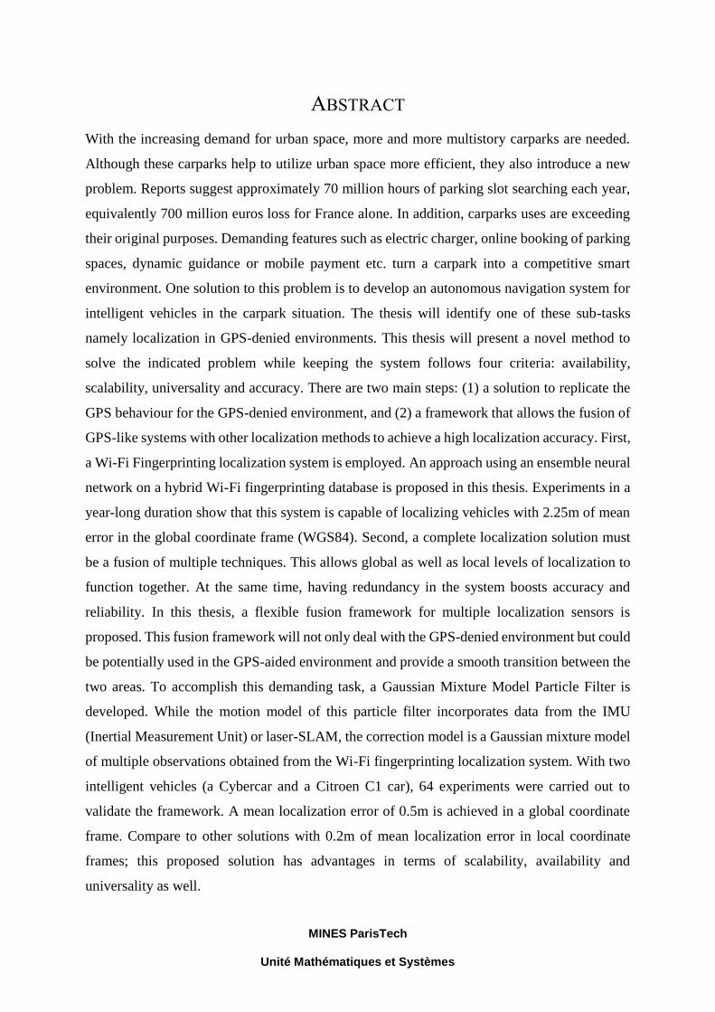
ABSTRACT
With the increasing demand for urban space, more and more multistory carparks are needed.
Although these carparks help to utilize urban space more efficient, they also introduce a new
problem. Reports suggest approximately 70 million hours of parking slot searching each year,
equivalently 700 million euros loss for France alone. In addition, carparks uses are exceeding
their original purposes. Demanding features such as electric charger, online booking of parking
spaces, dynamic guidance or mobile payment etc. turn a carpark into a competitive smart
environment. One solution to this problem is to develop an autonomous navigation system for
intelligent vehicles in the carpark situation. The thesis will identify one of these sub-tasks
namely localization in GPS-denied environments. This thesis will present a novel method to
solve the indicated problem while keeping the system follows four criteria: availability,
scalability, universality and accuracy. There are two main steps: (1) a solution to replicate the
GPS behaviour for the GPS-denied environment, and (2) a framework that allows the fusion of
GPS-like systems with other localization methods to achieve a high localization accuracy. First,
a Wi-Fi Fingerprinting localization system is employed. An approach using an ensemble neural
network on a hybrid Wi-Fi fingerprinting database is proposed in this thesis. Experiments in a
year-long duration show that this system is capable of localizing vehicles with 2.25m of mean
error in the global coordinate frame (WGS84). Second, a complete localization solution must
be a fusion of multiple techniques. This allows global as well as local levels of localization to
function together. At the same time, having redundancy in the system boosts accuracy and
reliability. In this thesis, a flexible fusion framework for multiple localization sensors is
proposed. This fusion framework will not only deal with the GPS-denied environment but could
be potentially used in the GPS-aided environment and provide a smooth transition between the
two areas. To accomplish this demanding task, a Gaussian Mixture Model Particle Filter is
developed. While the motion model of this particle filter incorporates data from the IMU
(Inertial Measurement Unit) or laser-SLAM, the correction model is a Gaussian mixture model
of multiple observations obtained from the Wi-Fi fingerprinting localization system. With two
intelligent vehicles (a Cybercar and a Citroen C1 car), 64 experiments were carried out to
validate the framework. A mean localization error of 0.5m is achieved in a global coordinate
frame. Compare to other solutions with 0.2m of mean localization error in local coordinate
frames; this proposed solution has advantages in terms of scalability, availability and
universality as well.
MINES ParisTech
Unité Mathématiques et Systèmes
ACKNOWLEDGEMENTS
I would like to thank my family, my wife Linh, my parents, my sister and our little cat for all
the support. No word can describe how much they mean to me.
To my supervisors, thank you! You all have been so patient and thoughtful with me. You gave
me this extraordinary opportunity at the beginning and accomplishing this thesis would not be
possible without your advices.
To my colleagues, Raoul, Anne, Jean-Marc, and the PhD gang, thank you! You all have been
fantastic. I could not ask for a better team.
And finally, to my future baby boy, this is for you!

MINES ParisTech
Unité Mathématiques et Systèmes
CONTENTS
1. INTRODUCTION ................................................................................................... 1
1.1 CONTEXT .................................................................................................................. 2
1.2 SCOPE ....................................................................................................................... 4
1.3 MAIN CONTRIBUTIONS ............................................................................................. 6
1.4 THESIS OVERVIEW .................................................................................................... 7
2. INTELLIGENT VEHICLES LOCALIZATION ............................................... 10
2.1 OVERVIEW OF INTELLIGENT VEHICLES LOCALIZATION .......................................... 14
2.2 GPS-BASED LOCALIZATION ................................................................................... 15
2.3 LASER-BASED LOCALIZATION ................................................................................ 20
2.3.1 Filter-based Laser SLAM ............................................................................... 21
2.3.2 Optimization-based Laser SLAM ................................................................... 23
2.4 VISION-BASED LOCALIZATION ............................................................................... 24
2.5 DEAD-RECKONING ................................................................................................. 25
2.6 INTELLIGENT VEHICLES LOCALIZATION IN GPS-DENIED ENVIRONMENTS ............. 27
2.6.1 Absolute Localization ..................................................................................... 27
2.6.2 Relative Localization ...................................................................................... 31
2.7 DISCUSSION ............................................................................................................ 32
3. WIRELESS SENSOR NETWORKS LOCALIZATION .................................. 36
3.1 INTRODUCTION ....................................................................................................... 37
3.2 LOCALIZATION STRATEGIES OVERVIEW ................................................................. 38
3.3 RANGE-BASED APPROACH ...................................................................................... 38
3.3.1 Time of Arrival ............................................................................................... 38
3.3.2 Angle of Arrival .............................................................................................. 40
3.3.3 Received Signal Strength Indicator ................................................................ 42
3.4 RANGE-FREE APPROACH ......................................................................................... 43
3.4.1 Distance Vector Hop ...................................................................................... 43
3.4.2 Approximate Point-in-Triangulation Test ...................................................... 45
3.4.3 Fingerprinting Localization ........................................................................... 45
3.4.4 Centroid Localization ..................................................................................... 47
3.5 DISCUSSION ............................................................................................................ 47
4. WI-FI FINGERPRINTING LOCALIZATION ................................................. 50
4.1 INTRODUCTION ....................................................................................................... 52
MINES ParisTech
Unité Mathématiques et Systèmes
4.2 RELATED WORKS ................................................................................................... 56
4.3 ENSEMBLE APPROACH FOR WI-FI FINGERPRINTING LOCALIZATION OF INTELLIGENT
VEHICLES ..................................................................................................................... 61
4.3.1 Hybrid Database Offline Phase ..................................................................... 62
4.3.2 Wi-Fi Ensemble Neural Network ................................................................... 65
4.4 EXPERIMENTS AND RESULTS .................................................................................. 70
4.4.1 Survey of the Wi-Fi Characteristics in the Experiment Area ......................... 72
4.4.2 Wi-Fi localization Experiments ...................................................................... 75
4.5 DISCUSSION ............................................................................................................ 78
5. FUSION STRATEGY FOR LOCALIZATION ENHANCEMENT ................ 81
5.1 INTRODUCTION ....................................................................................................... 83
5.2 THE PARTICLE FILTER ............................................................................................ 86
5.2.1 Initialization Step ........................................................................................... 87
5.2.2 Prediction Step ............................................................................................... 87
5.2.3 Correction Step .............................................................................................. 88
5.2.4 Selection & Resampling Step ......................................................................... 89
5.3 GAUSSIAN MIXTURE MODEL PARTICLE FILTER ..................................................... 90
5.3.1 Initialization Step ........................................................................................... 91
5.3.2 Correction Step .............................................................................................. 92
5.4 FUSION OF WI-FI FINGERPRINTING AND IMU ........................................................ 95
5.4.1 Inputs Synchronization ................................................................................... 96
5.4.2 Particles Propagation .................................................................................... 97
5.4.3 Motion model.................................................................................................. 97
5.4.4 Selection & Resampling ................................................................................. 98
5.5 FUSION OF WI-FI FINGERPRINTING, IMU AND LASER-SLAM ................................ 99
5.5.1 Evidential SLAM .......................................................................................... 100
5.5.2 PML-SLAM................................................................................................... 102
5.5.3 SLAM in Global Coordinate Frame ............................................................. 104
5.5.4 SLAM as Odometry Measurements .............................................................. 106
5.6 EXPERIMENTS AND RESULTS ................................................................................ 108
5.6.1 Wi-Fi Fingerprinting Localization and IMU Fusion ................................... 108
5.6.2 Wi-Fi Fingerprinting Localization, IMU and Laser-SLAM fusion .............. 118
5.7 DISCUSSION .......................................................................................................... 122

MINES ParisTech
Unité Mathématiques et Systèmes
6. CONCLUSION .................................................................................................... 126
6.1 THESIS MOTIVATION ............................................................................................. 127
6.2 THESIS CONTRIBUTIONS ........................................................................................ 128
6.3 FUTURE WORK ...................................................................................................... 130
6.4 CONCLUSION ........................................................................................................ 131
7. REFERENCES .................................................................................................... 133
8. APPENDIX 1: RÉSUMÉ .................................................................................... 149
9. APPENDIX 2: ABSTRACT ............................................................................... 162
MINES ParisTech
Unité Mathématiques et Systèmes
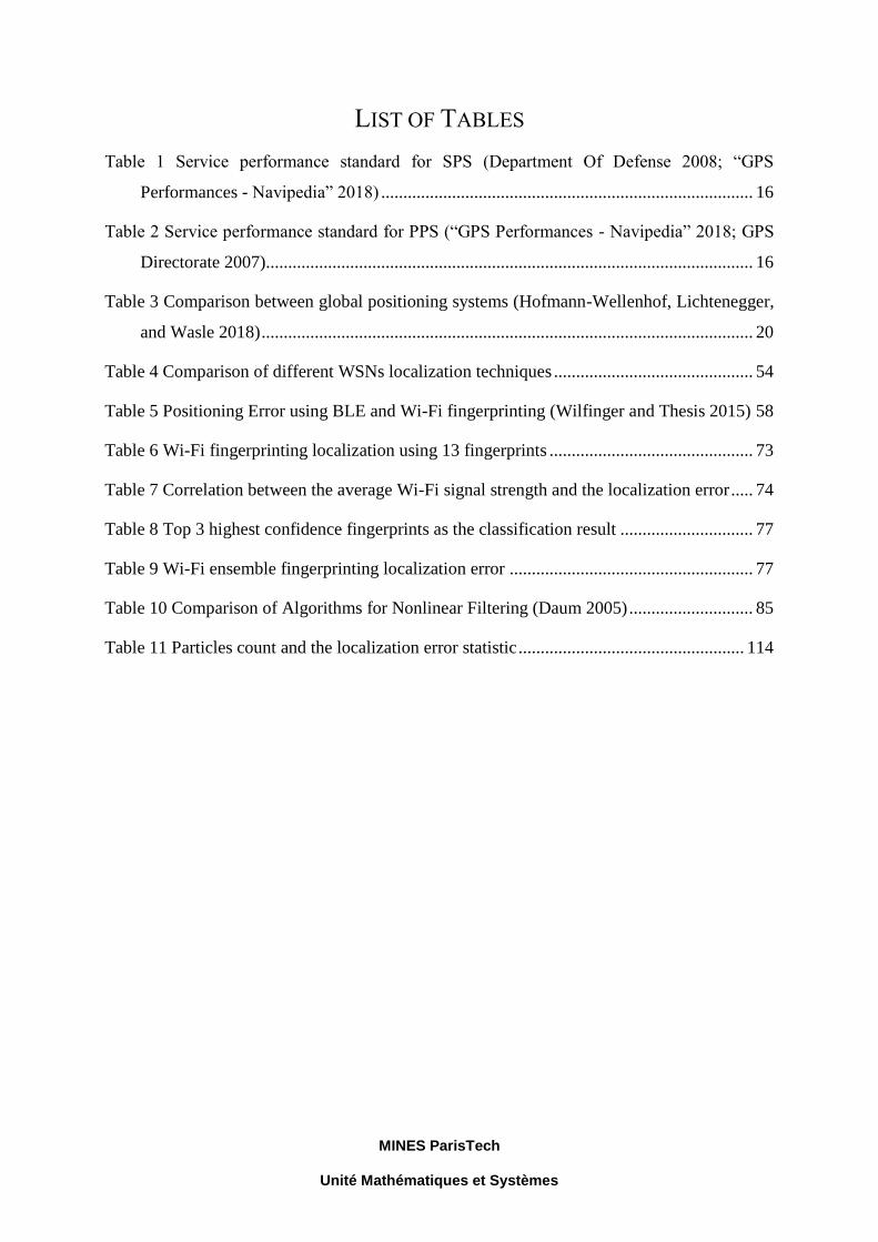
LIST OF TABLES
Table 1 Service performance standard for SPS (Department Of Defense 2008; “GPS
Performances - Navipedia” 2018) .................................................................................... 16
Table 2 Service performance standard for PPS (“GPS Performances - Navipedia” 2018; GPS
Directorate 2007).............................................................................................................. 16
Table 3 Comparison between global positioning systems (Hofmann-Wellenhof, Lichtenegger,
and Wasle 2018) ............................................................................................................... 20
Table 4 Comparison of different WSNs localization techniques ............................................. 54
Table 5 Positioning Error using BLE and Wi-Fi fingerprinting (Wilfinger and Thesis 2015) 58
Table 6 Wi-Fi fingerprinting localization using 13 fingerprints .............................................. 73
Table 7 Correlation between the average Wi-Fi signal strength and the localization error ..... 74
Table 8 Top 3 highest confidence fingerprints as the classification result .............................. 77
Table 9 Wi-Fi ensemble fingerprinting localization error ....................................................... 77
Table 10 Comparison of Algorithms for Nonlinear Filtering (Daum 2005) ............................ 85
Table 11 Particles count and the localization error statistic ................................................... 114
MINES ParisTech
Unité Mathématiques et Systèmes
LIST OF FIGURES
Figure 1.1 Parkmatic – Automated Parking System (“Parkmatic - Multi Parking” 2018) ........ 3
Figure 1.2 OneSITU – Parking Management System (“Parking Solutions - Solutions -
OneSITU” 2018) ................................................................................................................ 4
Figure 1.3 World Geodetic Coordinate System WGS84 (Malys et al. 2015) ............................ 5
Figure 2.1 Fusion of localization systems ................................................................................ 15
Figure 2.2 GPS principle .......................................................................................................... 16
Figure 2.3 The Galileo satellites navigation system commercial service architecture
(Fernández-Hernández et al. 2018) .................................................................................. 18
Figure 2.4 The kinematic high precision positioning results of Galileo (Ignacio, Irma, and
Guillermo 2015) ............................................................................................................... 19
Figure 2.5 The GLONASS accuracy evolution (“GLONASS Performances - Navipedia” 2018)
.......................................................................................................................................... 19
Figure 2.6 Graphical representation of (a) Full SLAM problem; (b) Online SLAM problem
(Bresson et al. 2017)......................................................................................................... 20
Figure 2.7 Particle Filter based Evidential SLAM (Trehard et al. 2014) ................................. 22
Figure 2.8 GraphSLAM visualization of large scale forest mapping (Pierzchała, Giguère, and
Astrup 2018) ..................................................................................................................... 23
Figure 2.9 GPS-aided SLAM for large scale uban mapping (Carlson, Thorpe, and Browning
2010)................................................................................................................................. 24
Figure 2.10 Edge-filtered map of the environment (Borges et al. 2010) ................................. 25
Figure 2.11 Camera image to edge image transformation (Borges et al. 2010) ...................... 25
Figure 2.12 Dead-reckoning and static map (Fouque et al. 2008) ........................................... 27
Figure 2.13 Graphical representation of SLAM with a static map (Wahl et al. 2015) ............ 28
Figure 2.14 2D map and LiDAR reading of the obstacle-free environment (Ibisch et al. 2013)
.......................................................................................................................................... 29
Figure 2.15 Sensor setup for camera-based carpark localization (Schwesinger et al. 2016) ... 30
MINES ParisTech
Unité Mathématiques et Systèmes
Figure 2.16 Flow chart of 3D map-matching based on particle filter (Bojja et al. 2013) ........ 31
Figure 2.17 Fisheye-based parking lot searching (Houben et al. 2013) ................................... 32
Figure 2.18 Two levels of localization system ......................................................................... 33
Figure 3.1 Two-way scheme of TOA ....................................................................................... 39
Figure 3.2 Angle of Arrival (AOA) localization method (Yin et al. 2016) ............................. 41
Figure 3.3 Angel of Arrival confidence zone ........................................................................... 41
Figure 3.4 Array Track localization error ................................................................................ 42
Figure 3.5 Signal propagation through obstacles (Dao et al. 2014) ......................................... 43
Figure 3.6 DV-Hop distance .................................................................................................... 44
Figure 3.7 Approximate point-in-triangulation test (F. Liu and Tan 2012) ............................. 45
Figure 3.8 Fingerprinting localization concept ........................................................................ 46
Figure 3.9 Centroid algorithm concept (Hongyang Chen et al. 2008) ..................................... 47
Figure 4.1 Fingerprints illustration........................................................................................... 54
Figure 4.2 iParking system architecture (J. Liu et al. 2012) .................................................... 56
Figure 4.3 Thondorf carpark (Wilfinger and Thesis 2015) ...................................................... 57
Figure 4.4 Time series for a test run (Wilfinger and Thesis 2015) .......................................... 57
Figure 4.5 Sensors setup and testing environment (Gikas et al. 2016) .................................... 59
Figure 4.6 The Universidad Carlos II de Madrid campus (Hernandez et al. 2017) ................. 59
Figure 4.7 General architecture of the system (Hernandez et al. 2017) ................................... 60
Figure 4.8 Cumulative Distribution of Error (Hernandez et al. 2017) ..................................... 60
Figure 4.9 Wi-Fi localization in urban area (Ang 2018) .......................................................... 61
Figure 4.10 Cumulative distribution of error in urban area (Ang 2018) .................................. 61
Figure 4.11 Online scan range for different speeds ................................................................. 62
Figure 4.12 Distance between two adjacent fingerprints ......................................................... 64
Figure 4.13 Ensemble of estimators motivation (Dietterich 2000) .......................................... 67
Figure 4.14 Fully connected neural network with 1 hidden layer ............................................ 68
MINES ParisTech
Unité Mathématiques et Systèmes
Figure 4.15 Boostrap hybrid database ...................................................................................... 69
Figure 4.16 Testing area in INRIA Rocquencourt campus ...................................................... 71
Figure 4.17 Blue Cybercar and Red Citroen C1 ...................................................................... 71
Figure 4.18 The Wi-Fi heat map of the testing area ................................................................. 72
Figure 4.19 13 Reference points in the environment ............................................................... 73
Figure 4.20Number of detected access points for each reference point ................................... 73
Figure 4.21 Distribution of localization error for each fingerprint .......................................... 74
Figure 4.22 Cumulative distribution of the localization error for fingerprints 1-9 .................. 75
Figure 4.23 The experiment area with 25 fingerprints ............................................................. 75
Figure 4.24 Localization result for 1 run .................................................................................. 77
Figure 5.1 Particle Filter Flowchart ......................................................................................... 88
Figure 5.2 Particle filter and Wi-Fi fingerprinting flowchart ................................................... 91
Figure 5.3 Gaussian Mixture Model Estimation ...................................................................... 93
Figure 5.4 Single Gaussian Model Estimation ......................................................................... 93
Figure 5.5 Gaussian Mixture Model in Practice 1 ................................................................... 94
Figure 5.6 Gaussian Mixture Model in Practice 2 ................................................................... 95
Figure 5.7 Gaussian Mixture Model Particle Filter with IMU and Wi-Fi fingerprinting ........ 96
Figure 5.8 Input Synchronization Timestamp .......................................................................... 96
Figure 5.9 General architecture for Evidential SLAM (Trehard et al. 2014) ......................... 101
Figure 5.10 Evidential SLAM test drive in KITTI database (Trehard et al. 2014) ................ 102
Figure 5.11 General flowchart of the PML-SLAM algorithm (Alsayed et al. 2015) ............ 103
Figure 5.12 Test drive on KITTI database with PML-SLAM (Alsayed et al. 2015) ............. 103
Figure 5.13 Deviation of distance and heading for PML SLAM (Alsayed et al. 2015) ........ 104
Figure 5.14 Fusion of laser-SLAM, Wi-Fi fingerprinting and IMU ...................................... 106
Figure 5.15 Laser-SLAM and IMU particles clouds .............................................................. 107

MINES ParisTech
Unité Mathématiques et Systèmes
Figure 5.16 True position during the initialization step: within fingerprint area (red) and outside
fingerprint area (blue)..................................................................................................... 109
Figure 5.17 Initial position within the defined fingerprint area case ..................................... 111
Figure 5.18 Experiment test run ............................................................................................. 111
Figure 5.19 Localization error with corresponding ground truth quality ............................... 112
Figure 5.20 Travel path with RTK GPS quality ..................................................................... 112
Figure 5.21 Initial position outside the defined fingerprint area case .................................... 113
Figure 5.22 Experiment test run ............................................................................................. 114
Figure 5.23 Initial position within a fingerprint area ............................................................. 115
Figure 5.24 Initial position outside a fingerprint area ............................................................ 115
Figure 5.25 Localization error histogram of all experiments ................................................. 116
Figure 5.26 Cumulative sum of errors for all experiments .................................................... 116
Figure 5.27 Localization error histogram (good initial position) ........................................... 117
Figure 5.28 Cumulative sum of localization error (good initial position) ............................. 117
Figure 5.29 laser-SLAM in Global Coordinate ...................................................................... 118
Figure 5.30 Fusion System (Wi-Fi and laser-SLAM) in the Global Coordinate Frame ........ 119
Figure 5.31 Localization error of fusion solution .................................................................. 120
Figure 5.32 Experiment test run ............................................................................................. 120
Figure 5.33 PML-SLAM online map ..................................................................................... 121
Figure 5.34 Evidential SLAM online map ............................................................................. 122

MINES ParisTech
Unité Mathématiques et Systèmes
LIST OF ABBREVIATIONS AND ACRONYMS
Abbreviation Full Name
AOA Angle of Arrival
APIT Approximate Point In Triangulation Test
CV Coefficient of Variation
DGPS Differential Global Positioning System
DV-hop Distance Vector Hop
EKF Extended Kalman Filter
EPS Effective Particle Size
FP Fingerprint
GMM Gaussian Mixture Model
GNSS Global Navigation Satellite System
GPS Global Positioning Systems
ICP Iterative Closest Points
IMU Inertial Measurement Unit
IoT Internet of Things
ITS Intelligent Transportation Systems
KNN K-Nearest Neighbours
OOI Object of Interest
PML Probabilistic Maximum Likelihood
PPS Precise Positioning Service
RIOs Road Infrastructure Objects
RMSE Root Mean Square Error
RSSI Received Signal Strength Indicator
MINES ParisTech
Unité Mathématiques et Systèmes
RTK Real-time Kinematic
SLAM Simultaneous Localization and Mapping
SPS Standard Positioning Service
SVM Support Vector Machine
TDOA Time Difference of Arrival
TOA Time of Arrival
V2I Vehicle to Infrastructure
WEFLS Wi-Fi Ensemble Fingerprinting Localization System
WLAN Wireless Local Area Network
WSNs Wireless Sensors Networks

1
1. INTRODUCTION
Résumé
Le chapitre présente la motivation, la portée et le but de la thèse. Cette thèse débute avec la
collaboration de deux unités de recherche, l’équipe RITS, l’INRIA France et l’institut MICA,
et est financée par le programme de bourses d’études 911 du gouvernement vietnamien. comme
autoroute, rues urbaines, etc. L’environnement sans GPS, qui est également un scénario
important pour les applications de véhicules intelligents, n’a pas encore été totalement traité.
Un environnement notable pour un tel scénario est un parking couvert. Cette thèse a pour
objectif de trouver une nouvelle solution au problème de localisation dans un environnement
sans GPS. Les solutions existantes pour ce scénario sont coûteuses à déployer ou ne permettent
pas de résoudre complètement le problème. Par conséquent, la solution doit être une méthode
de localisation globale qui permette une transition transparente entre la localisation
d’environnement assistée par GPS et celle qui est refusée par le GPS et satisfasse à quatre
critères: disponibilité, évolutivité, universalité et précision. Deux contributions principales sont
proposées: un système de localisation d'empreintes digitales d'ensemble Wi-Fi capable de
reproduire le comportement du GPS pour l'environnement sans GPS et un cadre de fusion de
filtres à particules mélangées gaussien permettant la fusion de techniques de localisation
multiples.
Chapter 1: Introduction -------------------------------------------------------------------------------------------------------------------
Nguyen Dinh Van - January 2019 2
1.1 Context
The thesis is conducted in collaboration of two research units: RITS team, INRIA France and
MICA Institute, Vietnam and funded by Vietnamese government scholarship program 911.
RITS (Robotics for Intelligent Transportation Systems) team is a multidisciplinary project team
at INRIA, working on Robotics for Intelligent Transportation Systems. The team focuses on
enabling advanced intelligent robotics systems for autonomous and sustainable mobility. One
notable application is Intelligent Vehicles (IVs) which can navigate autonomously in different
environments.
MICA (Multimedia, Information Communication and Application) International Research
Institute is established in Vietnam by CNRS, Grenoble INP and Hanoi University of Science
and Technology. One of its research interests is indoor localization in smart environments using
wireless sensors networks. The main objective of this research is to enable indoor navigation
for targets such as humans or robots.
With the increasing demand for urban space, more and more multistory carparks are needed.
Although these carparks help to utilize urban space more efficient, they also introduce a new
problem. Reports in (Belloche 2015; Gantelet and Lefauconnier 2006) suggest the average
searching time for a free slot in a carpark in Paris or Lyon is 20 minutes and can be as high as
40 minutes for some districts. This leads to approximately 70 million hours of searching each
year, equivalently 700 million euros loss for France alone. In addition, carparks uses are
exceeding their original purposes. Demanding features such as electric charger, online booking
of parking spaces, dynamic guidance or mobile payment etc. turn a carpark into a competitive
smart environment. Furthermore, 20 most populous cities in France must engage an open data
approach from October 1st, 2018 in accordance with the law for a digital Republic (“Loi Du 7
Octobre 2016 Pour Une République Numérique” 2016). This introduces a great chance to invent
a new way to calculate traffic flow, develop intelligent services such as intelligent car parks
(“Parking at the Service of Connected Urban Mobility and a Sustainable City - The Urban
Mobility Blog” 2018).
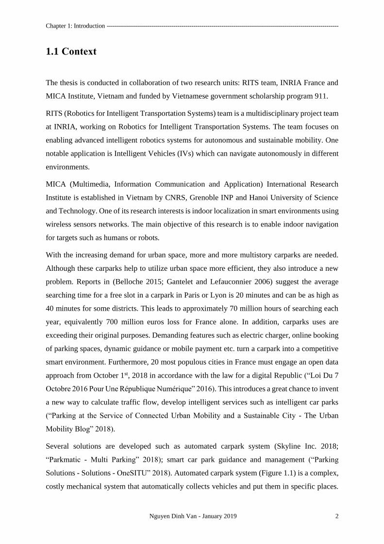
Several solutions are developed such as automated carpark system (Skyline Inc. 2018;
“Parkmatic - Multi Parking” 2018); smart car park guidance and management (“Parking
Solutions - Solutions - OneSITU” 2018). Automated carpark system (Figure 1.1) is a complex,
costly mechanical system that automatically collects vehicles and put them in specific places.
Chapter 1: Introduction -------------------------------------------------------------------------------------------------------------------
Nguyen Dinh Van - January 2019 3
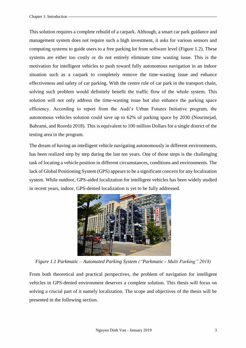
This solution requires a complete rebuild of a carpark. Although, a smart car park guidance and
management system does not require such a high investment, it asks for various sensors and
computing systems to guide users to a free parking lot from software level (Figure 1.2). These
systems are either too costly or do not entirely eliminate time wasting issue. This is the
motivation for intelligent vehicles to push toward fully autonomous navigation in an indoor
situation such as a carpark to completely remove the time-wasting issue and enhance
effectiveness and safety of car parking. With the centre role of car park in the transport chain,
solving such problem would definitely benefit the traffic flow of the whole system. This
solution will not only address the time-wasting issue but also enhance the parking space
efficiency. According to report from the Audi’s Urban Futures Initiative program, the
autonomous vehicles solution could save up to 62% of parking space by 2030 (Nourinejad,
Bahrami, and Roorda 2018). This is equivalent to 100 million Dollars for a single district of the
testing area in the program.
The dream of having an intelligent vehicle navigating autonomously in different environments,
has been realized step by step during the last ten years. One of those steps is the challenging
task of locating a vehicle position in different circumstances, conditions and environments. The
lack of Global Positioning System (GPS) appears to be a significant concern for any localization
system. While outdoor, GPS-aided localization for intelligent vehicles has been widely studied
in recent years, indoor, GPS-denied localization is yet to be fully addressed.
Figure 1.1 Parkmatic – Automated Parking System (“Parkmatic - Multi Parking” 2018)
From both theoretical and practical perspectives, the problem of navigation for intelligent
vehicles in GPS-denied environment deserves a complete solution. This thesis will focus on
solving a crucial part of it namely localization. The scope and objectives of the thesis will be
presented in the following section.
Chapter 1: Introduction -------------------------------------------------------------------------------------------------------------------
Nguyen Dinh Van - January 2019 4
Figure 1.2 OneSITU – Parking Management System (“Parking Solutions - Solutions -
OneSITU” 2018)
1.2 Scope
Autonomous navigation for an intelligent vehicle is a considerable task consisting of multiples
sub-tasks. Rather than trying to find a complete solution at once, it is essential to identify each
of these sub-tasks and deal with them separately. The thesis will identify one of these sub-tasks
as follows.
In this thesis, the targeted environments are the one without GPS signal such as: indoor carpark.
The targeted environment can also be extended to places with poor GPS signal and low
movement speed such as industrial factory, university campus or outdoor carpark. Throughout
this thesis, the term GPS-denied environment will be defined as an environment with poor or
no GPS signal and GPS-aided environment refers to the one with good reception of GPS signal.
At the same time, by targeting environment such as carpark, university campus, the average
movement speed of vehicles is expected to be around 3m/s (Belloche 2015). This is due to the
nature of these environments conditions as well as speed regulation applied. In fact, in recent
demonstrations of companies like Audi, BMW, etc. for autonomous carpark navigation
systems, vehicles are operated at around 10km/h. Understanding the vehicle's dynamics in the
localization problem will help to accurately identify advantages/ disadvantages of different
positioning methods.
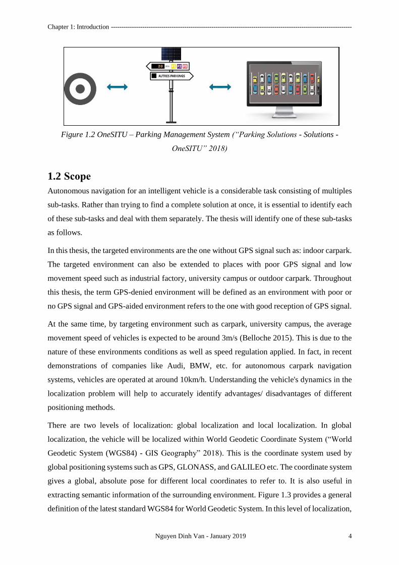
There are two levels of localization: global localization and local localization. In global
localization, the vehicle will be localized within World Geodetic Coordinate System (“World
Geodetic System (WGS84) - GIS Geography” 2018). This is the coordinate system used by
global positioning systems such as GPS, GLONASS, and GALILEO etc. The coordinate system
gives a global, absolute pose for different local coordinates to refer to. It is also useful in
extracting semantic information of the surrounding environment. Figure 1.3 provides a general
definition of the latest standard WGS84 for World Geodetic System. In this level of localization,
Chapter 1: Introduction -------------------------------------------------------------------------------------------------------------------
Nguyen Dinh Van - January 2019 5
the main objectives are to offer semantic data as well as a global reference frame thus
localization accuracy is not necessary to be in centimetres. On the other hand, local localization
refers to a local coordinate localization where accuracy level is supposed to be high. This level
of localization is responsible for accurate navigation and real-time obstacle avoidance. In
intelligent vehicles navigation, both levels of localization are required to accomplish the task
of navigation in different environment setups.
Figure 1.3 World Geodetic Coordinate System WGS84 (Malys et al. 2015)
With multiple sensors running on different local coordinates, it is critical to have a global frame
to express those sensors outputs together. In the GPS-denied environment, the lack of GPS
signal not only omits the essential global coordinate reference but also introduces a significant
gap in the transition phase between GPS-aided and GPS-denied environments. This thesis aims
to provide a global localization level method for GPS-denied environment. The proposed
solution should be able to replicate GPS signal behaviour for the indoor environment.
Also, a fusion framework is proposed so that other local localization techniques can be fused
into the global frame. This allows the system to achieve both local and global levels of
localization. In addition, this framework should be generic that it could be potentially applied
for both GPS-aided and GPS-denied environments thus allows seamless navigation transition
between these two environments.
With respect to the primary target of carpark environment, the system must comply with the
following requirements:
- Availability: The system should be easily deployable on existing infrastructure of a
carpark with limited requirements of changes in structures, hardware or software.
- Scalability: The system should be extensible and scalable in large scale.
Chapter 1: Introduction -------------------------------------------------------------------------------------------------------------------
Nguyen Dinh Van - January 2019 6
- Universality: there should be no specific hardware/ firmware changes other than off-
shelf devices. This removes the need for dedicated sensors to be mounted in different
carparks in order for the system to work.
- Accuracy: While ideally the system should be accurate in order of centimetres, in terms
of global localization for carpark situation, it is not necessary to be so. Methods such as
Laser-SLAM (Simultaneous Localization and Mapping) or vision based localization can
deal well with local accuracy. Still, the system accuracy should be able to identify
vehicle positioning within a parking plot. According to French standard “Norme NF P
91-100” (“Norme Francaise, Parcs de Stationnement a Usage Privatif” 1996), the
minimum width for a parking spot is 1.80m. This should be the upper bound of the
system accuracy. The final fusion localization system in this thesis is expected to be
within 0.5m of mean localization error. Ideally, the localization error of a fully
autonomous vehicle is under 0.2m (Ziegler et al. 2014).
1.3 Main Contributions
The thesis has two main contributions. First, a novel Wi-Fi Ensemble Fingerprinting
Localization System (WEFLS) for GPS-denied environment to replace the need of GPS signal.
Second, a framework for the fusion of multiple localization methods such as: GPS based, IMU
based, WEFLS based, laser-SLAM based.
There are currently no de facto standards for GPS-denied environment positioning systems
design as a global solution similar to the one used in the GPS-aided environment (e.g. GPS,
GLONASS, etc.). Regarding intelligent vehicle navigation in the carpark, several solutions are
proposed including: laser-SLAM with static map matching (Wahl et al. 2015), Embedded
LIDAR sensors in the environment (Ibisch et al. 2013), 3D map matching using vision sensors
(Bojja et al. 2013) or detection of parking lot using vision sensors (Houben et al. 2013) etc.
While these studies may allow up to 10cm of localization precision, they also come with high
cost or requirements such as: costly setup of sensors, complex environment map required, and
no global coordinate transformation addressed. An in-depth review of these studies will be
presented in chapter 2.
First, this thesis will present a novel method for GPS-denied environment localization using
wireless sensors networks, more specifically a Wi-Fi fingerprinting localization system. The
method makes use of existing Wi-Fi infrastructure (Wi-Fi Access Points – APs, Wi-Fi receiver)
to determine the target position based on an offline mapping phase. The main argument of this
Chapter 1: Introduction -------------------------------------------------------------------------------------------------------------------
Nguyen Dinh Van - January 2019 7
method is that the combination of Wi-Fi signal strengths from multiple static APs in the
environment for one position is unique. By learning these unique features for several key
positions in the environment, one can estimate its location just by scanning Wi-Fi signals
strengths.
Although Wi-Fi fingerprinting localization system is already a popular approach for indoor
localization, so far it only targets pedestrian walking speed. The advantages of this method are
its availability, scalability and universal characteristics where off the shelf hardware like Wi-Fi
receivers and Wi-Fi access points are used without any modification. These sensors are also
expected to be widely available nowadays in urban area. One main concern of this method is
the low sampling frequency of Wi-Fi scan. In general, the time to complete a scan of Wi-Fi
signals in a particular environment is around 1 second (1Hz). At 1.0 to 1.6m/s of human walking
speed (Harkema, Behrman, and Barbeau 2012), this sampling frequency is adequate to deliver
real-time localization results. However, as the thesis aims to target intelligent vehicles in the
carpark at 3m/s, the classic approach of the Wi-Fi fingerprinting method is insufficient. Thus,
an original approach using ensemble neural network on Wi-Fi fingerprinting method is
proposed in this thesis.
Secondly, a complete localization solution must be a fusion of multiple techniques. This allows
global as well as local levels of localization to function together. At the same time, having
redundancy in the system boosts accuracy and reliability. In this thesis, a flexible fusion
framework for multiple localization sensors is proposed. This fusion framework will not only
deal with the GPS-denied environment but could be potentially used in the GPS-aided
environment and provide a smooth transition between the two areas.
1.4 Thesis Overview
Following this introduction, the thesis has 5 more chapters presented as follows:
- Chapter 2: A brief overview of intelligent vehicles localization, particularly, localization in
the GPS-denied environment. The two categories of localization methods: absolute
localization and relative localization are reviewed and discussed.
- Chapter 3: A summary of Wireless Sensors Networks and its strategies for localization. Two
main strategies of this approach are range-based and range-free localization. This chapter
will provide discussion to highlight the motivation of using WSNs in intelligent localization
for GPS-denied environment.
Chapter 1: Introduction -------------------------------------------------------------------------------------------------------------------
Nguyen Dinh Van - January 2019 8
- Chapter 4: The core algorithm of the preferred WSNs localization strategy is presented. The
Wi-Fi fingerprinting localization method is introduced with critical improvement to adapt to
intelligent vehicle dynamics.
- Chapter 5: To enhance localization accuracy as well as frequency, a data fusion model is
proposed using Gaussian Mixture Model and Particle Filter. This strategy is also capable of
providing a smooth transition from the GPS-aided environment to GPS-denied environment.
The model is then verified by fusing Wi-Fi Fingerprinting localization with IMU and PML-
SLAM.
- Chapter 6: A conclusion of the thesis. It also highlights possible future work for this thesis
and discusses multiple perspectives regarding the results obtained.

Chapter 1: Introduction -------------------------------------------------------------------------------------------------------------------
Nguyen Dinh Van - January 2019 9
10
2. INTELLIGENT VEHICLES LOCALIZATION
Résumé
Dans ce chapitre, quelques techniques générales pour la localisation de véhicules intelligents
sont examinées. En outre, une étude des solutions existantes pour la localisation de véhicules
intelligents dans des environnements sans GPS est présentée.
En général, les techniques de localisation IV peuvent être divisées en deux catégories: la
localisation globale et la localisation locale. Souvent, la catégorie de localisation globale est
une méthode de localisation basée sur GNSS. Ces méthodes utilisent les signaux satellites pour
déterminer les informations de position 3D du récepteur dans une référence globale (telle que
WGS84). Le terme GPS fait référence au système de positionnement global qui est régi par les
États-Unis d'Amérique. Il existe d'autres systèmes mondiaux de navigation par satellite (GNSS)
tels que GLONASS (Russie), Galileo (Europe) et Beidou (Chine). Pour simplifier le problème,
la thèse se concentrera sur les performances du GPS en tant que représentant d'autres GNSS.
Le principe de calcul de la position du récepteur est basé sur la connaissance des positions des
satellites, puis sur la déduction des «pseudo-distances» respectives entre ces satellites et le
récepteur, comme illustré à la figure 2.2. Ici, le terme "pseudo-distance" se réfère à la distance
calculée entre les satellites et le récepteur mobile. Étant donné que les satellites se déplacent
constamment, cette distance n’est pas une valeur fixe. Pour calculer la position 3D d'un
récepteur, il faut au moins quatre satellites. Vous trouverez un aperçu du système GPS dans
(Hofmann-Wellenhof, Lichtenegger et Wasle 2018).
Il existe deux niveaux de services GPS, à savoir le service de positionnement standard (SPS) et
le service de positionnement précis (PPS). Alors que SPS est accessible aux utilisateurs publics,
les PPS de haute précision ne sont accessibles qu'aux utilisateurs autorisés (personnel militaire,

Chapter 2: Intelligent Vehicles Localization ------------------------------------------------------------------------------------------
Nguyen Dinh Van - January 2019 11
agents de l'État). Le tableau 1 et le tableau 2 récapitulent les performances SPS et PPS. En
général, SPS fournit une erreur de localisation maximale de 7,8 m dans 95% des cas, et le
système PPS offre une meilleure précision avec une erreur de localisation maximale de 5,9 m
dans 95% des heures. temps. En outre, la précision verticale devrait être inférieure à la précision
horizontale dans toutes les mesures GPS. Dans le meilleur des cas, une solution DGPS de haute
précision appelée GPS cinématique en temps réel (RTK GPS) peut offrir une précision de
quelques centimètres. Cependant, le procédé nécessite des stations de base dédiées, des
capteurs, des signaux GPS continus et un prix excessif pour le déploiement et la maintenance.
Cela rend le RTK non adapté à la plupart des applications urbaines («Real Time Kinematics -
Navipedia» 2018).
À l'instar des États-Unis, l'Union européenne a également mis au point un système de
positionnement global appelé Galileo, destiné à fournir un système de positionnement global
indépendant de haute précision aux pays européens. Le système est censé aider les pays de l’UE
à ne pas compter sur le chinois BeiDou, le russe GLONASS ou, plus important encore, sur le
GPS américain. Dans de bonnes conditions, telles que des satellites pleinement fonctionnels
(jusqu'à 30 unités), une vision claire du récepteur aux satellites, etc., le libre accès libre pour la
navigation du système Galileo à la frontière de l'UE devrait être d'environ 4 mètres de précision
(«Galileo Introduction générale - Navipedia ”2018). Le GLONASS développé par la Russie
dans les années 1980 est un autre système qui mérite d'être mentionné. En 2010, le GLONASS
couvrait l'ensemble du territoire russe, puis après octobre 2011, la couverture mondiale est
atteinte. L'évolution de la précision de positionnement du GLONASS est illustrée à la figure
2.5. Jusqu'à présent, sous un ciel statique, la précision du GLONASS pour l'accès public était
de 2,8 mètres. Vous trouverez une comparaison rapide des différents systèmes de localisation
globale dans le tableau 3.
Une méthode de localisation locale notable est la localisation au laser. En utilisant une
technique de télémètre basée sur les rayons laser, le capteur estime avec précision la distance
aux autres objets de l'environnement. Le LiDAR (James Eddy 2017) (détection de la lumière et
télémétrie) est une forme importante de capteur laser qui déclenche des faisceaux laser en
continu dans l'environnement. Cela aide à estimer la distance aux obstacles environnants et
permet de cartographier l'environnement à haute résolution. Lorsqu'il s'agit de capteur laser, la
majorité de ses algorithmes de localisation impliquent la résolution totale ou partielle d'un
problème de localisation et de cartographie simultanées (Smith et Cheeseman 2018), (Durrant-
Whyte et Bailey 2006), (Dellaert et al. 2018) . L’objectif du SLAM est d’estimer la trajectoire
Chapter 2: Intelligent Vehicles Localization ------------------------------------------------------------------------------------------
Nguyen Dinh Van - January 2019 12
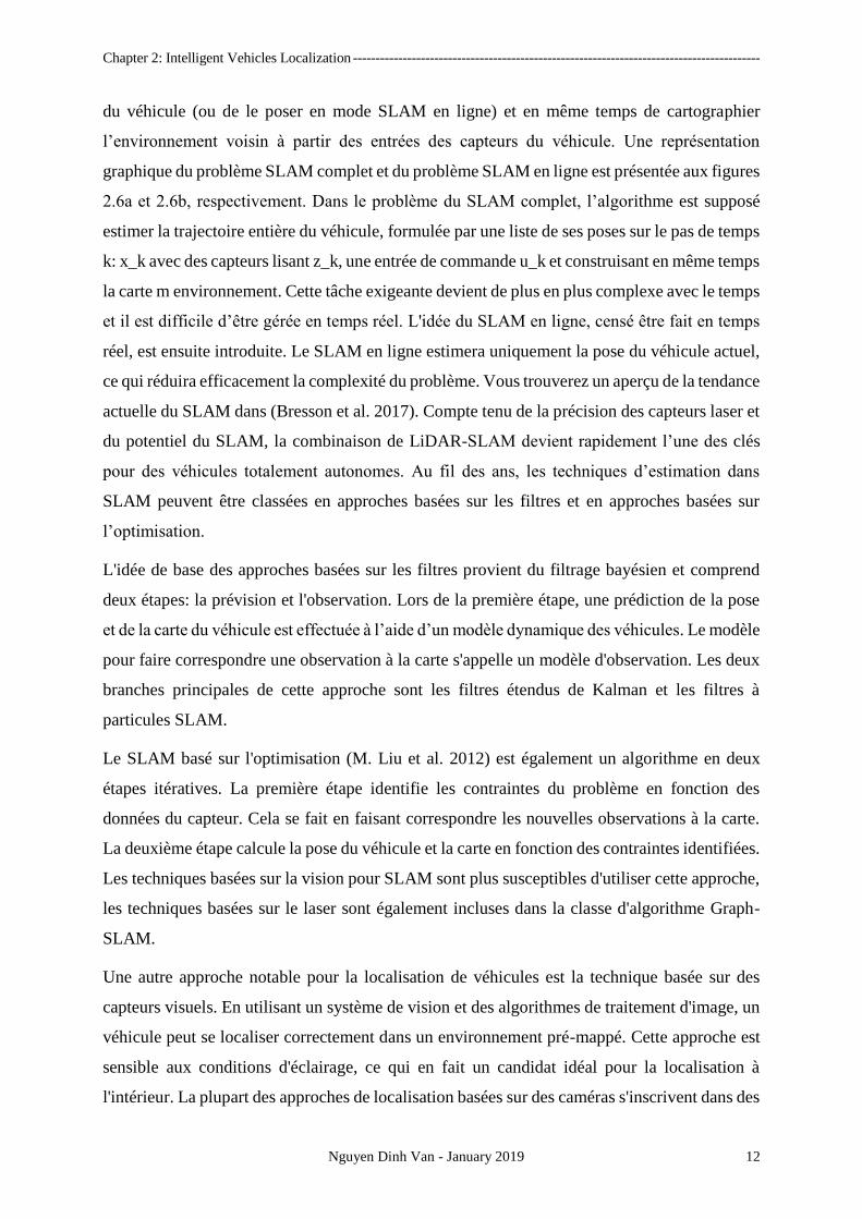
du véhicule (ou de le poser en mode SLAM en ligne) et en même temps de cartographier
l’environnement voisin à partir des entrées des capteurs du véhicule. Une représentation
graphique du problème SLAM complet et du problème SLAM en ligne est présentée aux figures
2.6a et 2.6b, respectivement. Dans le problème du SLAM complet, l’algorithme est supposé
estimer la trajectoire entière du véhicule, formulée par une liste de ses poses sur le pas de temps
k: x_k avec des capteurs lisant z_k, une entrée de commande u_k et construisant en même temps
la carte m environnement. Cette tâche exigeante devient de plus en plus complexe avec le temps
et il est difficile d’être gérée en temps réel. L'idée du SLAM en ligne, censé être fait en temps
réel, est ensuite introduite. Le SLAM en ligne estimera uniquement la pose du véhicule actuel,
ce qui réduira efficacement la complexité du problème. Vous trouverez un aperçu de la tendance
actuelle du SLAM dans (Bresson et al. 2017). Compte tenu de la précision des capteurs laser et
du potentiel du SLAM, la combinaison de LiDAR-SLAM devient rapidement l’une des clés
pour des véhicules totalement autonomes. Au fil des ans, les techniques d’estimation dans
SLAM peuvent être classées en approches basées sur les filtres et en approches basées sur
l’optimisation.
L'idée de base des approches basées sur les filtres provient du filtrage bayésien et comprend
deux étapes: la prévision et l'observation. Lors de la première étape, une prédiction de la pose
et de la carte du véhicule est effectuée à l’aide d’un modèle dynamique des véhicules. Le modèle
pour faire correspondre une observation à la carte s'appelle un modèle d'observation. Les deux
branches principales de cette approche sont les filtres étendus de Kalman et les filtres à
particules SLAM.
Le SLAM basé sur l'optimisation (M. Liu et al. 2012) est également un algorithme en deux
étapes itératives. La première étape identifie les contraintes du problème en fonction des
données du capteur. Cela se fait en faisant correspondre les nouvelles observations à la carte.
La deuxième étape calcule la pose du véhicule et la carte en fonction des contraintes identifiées.
Les techniques basées sur la vision pour SLAM sont plus susceptibles d'utiliser cette approche,
les techniques basées sur le laser sont également incluses dans la classe d'algorithme Graph-
SLAM.
Une autre approche notable pour la localisation de véhicules est la technique basée sur des
capteurs visuels. En utilisant un système de vision et des algorithmes de traitement d'image, un
véhicule peut se localiser correctement dans un environnement pré-mappé. Cette approche est
sensible aux conditions d'éclairage, ce qui en fait un candidat idéal pour la localisation à
l'intérieur. La plupart des approches de localisation basées sur des caméras s'inscrivent dans des

Chapter 2: Intelligent Vehicles Localization ------------------------------------------------------------------------------------------
Nguyen Dinh Van - January 2019 13
types de méthodes basées sur l'appariement de cartes. Dans ces approches, une carte détaillée
de l'environnement est construite dans une phase hors ligne. Sur la base de l'entrée de caméra
de phase en ligne et de la carte hors ligne, l'emplacement du véhicule est calculé. Semblable au
laser SLAM, le SLAM visuel est une approche populaire pour la localisation de véhicules
intelligents. Le concept SLAM reste le même que dans le SLAM laser, mais dans ce cas, un
ensemble de caméras est monté sur le véhicule pour capturer non seulement des images mais
également pour mesurer la profondeur de la scène.
Le calcul à mort est un processus d’estimation de la pose actuelle d’un véhicule à l’aide d’une
pose préalablement déterminée et du modèle dynamique du véhicule. À l’origine, il s’agissait
d’une approche développée pour les applications marines et qui est maintenant utilisée dans
divers domaines tels que la navigation aérienne, le suivi des piétons ou la navigation autonome
par robot. L'algorithme de calcul à rebours utilise différentes configurations de capteurs. Le
calcul à mort avec unités de mesure inertielle (IMU) est largement utilisé dans la navigation de
véhicules spatiaux, de navires de mer ou de véhicules terrestres. IMU a généralement des
gyroscopes à trois axes et des accélérateurs pour mesurer la vitesse angulaire et la vitesse de
déplacement de l'objet attaché.
L'un des inconvénients du GPS est sa disponibilité dans les scénarios urbains. Le plus souvent,
les signaux GPS sont perdus ou mal reçus dans un tunnel, un parking ou lorsque le récepteur
est entouré de bâtiments, obstruant ainsi la visibilité directe des satellites. Les signaux GPS
standard souffrent également de l'effet de trajets multiples qui pourrait entraîner une erreur de
localisation supplémentaire de 8 m (Kos, Markezic et Pokrajcic 2010). Néanmoins, le GPS (et
les autres GNSS) joue un rôle essentiel dans la localisation, en particulier à l’échelle mondiale,
car il s’agit du seul système de positionnement qui affiche directement dans le repère global.
Sans ces coordonnées de référence globales, chaque véhicule intelligent fonctionnera selon ses
propres coordonnées locales. Aucune communication ni coopération n'est possible.
Au cours des dernières années, la communauté de recherche sur les véhicules intelligents a
développé plusieurs systèmes dédiés à la localisation dans les zones interdites de GPS en
général et les parkings en particulier. En raison du manque de signaux GPS, la plupart des
solutions de localisation dans ce domaine se situent au niveau de la localisation locale. En
fonction du choix du système de coordonnées de référence, ces travaux peuvent être classés en
deux classes: méthodes de localisation absolue (ou basées sur une carte) et méthodes de
localisation relative (autocentrées, sans carte). Les travaux récents des deux classes seront
étudiés dans les sections suivantes.
Chapter 2: Intelligent Vehicles Localization ------------------------------------------------------------------------------------------
Nguyen Dinh Van - January 2019 14
Dans l'approche du positionnement absolu, il est nécessaire qu'une carte de l'environnement
soit connue au préalable par le véhicule. Cette carte comprend deux composants principaux: les
objets statiques qui contribuent à la structure de la carte (route, murs, portes, etc.) et les objets
dynamiques qui constituent des obstacles dans l'environnement (autres véhicules, piétons, etc.
.) Selon la solution, la carte peut contenir les deux ou uniquement des objets statiques.
Contrairement à la localisation absolue, la localisation relative ne nécessite pas une carte
détaillée de l'environnement. L’approche vise à estimer la position du véhicule par rapport aux
objets locaux environnants tels que les autres véhicules, le marquage des voies, etc.
Parmi ces deux approches, la méthode cartographique semble beaucoup plus précise. Un
système bien défini peut localiser des véhicules avec une précision allant jusqu'à 0,1 m.
Toutefois, pour ceux qui disposent d’une carte détaillée de l’environnement, la résolution et la
précision des informations cartographiques ont une influence considérable sur l’erreur de
localisation. Malheureusement, plus la résolution est élevée, plus la solution est complexe et
moins évolutive. Ainsi, une nouvelle solution pour ce scénario est requise.
2.1 Overview of Intelligent Vehicles Localization
Localization is a task of determining an object’s pose (e.g. coordinate, heading angle) or the
spatial relationship among objects. This is an essential task for an autonomous navigation a
vehicle has to achieve (Eskandarian 2012). Only by knowing precisely the location of itself in
either a local or a global map, then action such as path planning or obstacles avoidance can be
carried out. Often, this task is accomplished through a set of dedicated sensors (on vehicle
sensors or environment sensors). The process of combining these sensors inputs to infer the
vehicle’s position is called sensor fusion.
There are two levels of localization for intelligent vehicles: global level and local level. The
global level localization often results in the vehicle’s pose in the global coordinates frame (e.g.
WGS84, NAVD88, ETRS89, etc.) and offers a broad view of vehicle’s location and context.
The accuracy of this localization level is not required to be in the order of centimetres. Instead,
a raw but stable estimation of the vehicle’s absolute location is sufficient. One example of this
level of localization is GNSS-based localization methods. The local level of localization is
usually expressed in an arbitrary local reference coordinate frame. This level of localization is
responsible for accurately determining the spatial relationship of the vehicle with other objects
in the environment. Some notable methods for this level of localization are laser-SLAM,
camera-based map matching, dead-reckoning, etc.
Chapter 2: Intelligent Vehicles Localization ------------------------------------------------------------------------------------------
Nguyen Dinh Van - January 2019 15
Data Fusion
Global Level LocalizationGPS-aided methods
Local Level Localization
𝑿 𝑮𝒍𝒐𝒃𝒂𝒍
𝑿 𝑳𝒐𝒄𝒂𝒍
𝑿
Figure 2.1 Fusion of localization systems
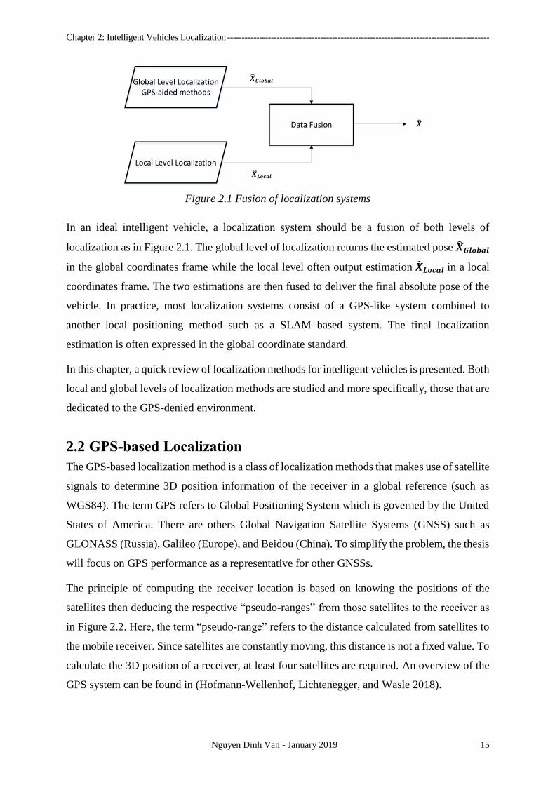
In an ideal intelligent vehicle, a localization system should be a fusion of both levels of
localization as in Figure 2.1. The global level of localization returns the estimated pose 𝑿 𝑮𝒍𝒐𝒃𝒂𝒍
in the global coordinates frame while the local level often output estimation 𝑿 𝑳𝒐𝒄𝒂𝒍 in a local
coordinates frame. The two estimations are then fused to deliver the final absolute pose of the
vehicle. In practice, most localization systems consist of a GPS-like system combined to
another local positioning method such as a SLAM based system. The final localization
estimation is often expressed in the global coordinate standard.
In this chapter, a quick review of localization methods for intelligent vehicles is presented. Both
local and global levels of localization methods are studied and more specifically, those that are
dedicated to the GPS-denied environment.
2.2 GPS-based Localization
The GPS-based localization method is a class of localization methods that makes use of satellite
signals to determine 3D position information of the receiver in a global reference (such as
WGS84). The term GPS refers to Global Positioning System which is governed by the United
States of America. There are others Global Navigation Satellite Systems (GNSS) such as
GLONASS (Russia), Galileo (Europe), and Beidou (China). To simplify the problem, the thesis
will focus on GPS performance as a representative for other GNSSs.
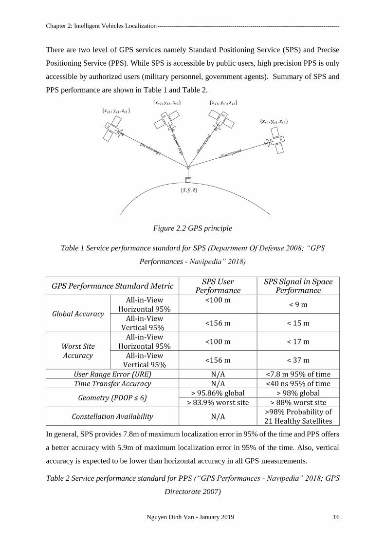
The principle of computing the receiver location is based on knowing the positions of the
satellites then deducing the respective “pseudo-ranges” from those satellites to the receiver as
in Figure 2.2. Here, the term “pseudo-range” refers to the distance calculated from satellites to
the mobile receiver. Since satellites are constantly moving, this distance is not a fixed value. To
calculate the 3D position of a receiver, at least four satellites are required. An overview of the
GPS system can be found in (Hofmann-Wellenhof, Lichtenegger, and Wasle 2018).
Chapter 2: Intelligent Vehicles Localization ------------------------------------------------------------------------------------------
Nguyen Dinh Van - January 2019 16
There are two level of GPS services namely Standard Positioning Service (SPS) and Precise
Positioning Service (PPS). While SPS is accessible by public users, high precision PPS is only
accessible by authorized users (military personnel, government agents). Summary of SPS and
PPS performance are shown in Table 1 and Table 2.
𝑥𝑠1,𝑦𝑠1 , 𝑧𝑠1
𝑥𝑠2,𝑦𝑠2 , 𝑧𝑠2 𝑥𝑠3,𝑦𝑠3 , 𝑧𝑠3
𝑥𝑠4,𝑦𝑠4 , 𝑧𝑠4
𝑥 ,𝑦 , 𝑧
Figure 2.2 GPS principle
Table 1 Service performance standard for SPS (Department Of Defense 2008; “GPS
Performances - Navipedia” 2018)
GPS Performance Standard Metric SPS User
Performance SPS Signal in Space
Performance
Global Accuracy
All-in-View Horizontal 95%
<100 m
< 9 m
All-in-View Vertical 95%
<156 m < 15 m
Worst Site Accuracy
All-in-View Horizontal 95%
<100 m < 17 m
All-in-View Vertical 95%
<156 m < 37 m
User Range Error (URE) N/A <7.8 m 95% of time Time Transfer Accuracy N/A <40 ns 95% of time
Geometry (PDOP ≤ 6) > 95.86% global > 98% global
> 83.9% worst site > 88% worst site
Constellation Availability N/A >98% Probability of 21 Healthy Satellites
In general, SPS provides 7.8m of maximum localization error in 95% of the time and PPS offers
a better accuracy with 5.9m of maximum localization error in 95% of the time. Also, vertical
accuracy is expected to be lower than horizontal accuracy in all GPS measurements.
Table 2 Service performance standard for PPS (“GPS Performances - Navipedia” 2018; GPS
Directorate 2007)
Chapter 2: Intelligent Vehicles Localization ------------------------------------------------------------------------------------------
Nguyen Dinh Van - January 2019 17
GPS Performance Standard Metric SPS User
Performance SPS Signal in Space
Performance
Global Accuracy
All-in-View Horizontal 95%
<36 m < 13 m
All-in-View Vertical 95%
<77 m < 22m
User Range Error (URE) N/A <5.9 m 95% of time Time Transfer Accuracy N/A <40 ns 95% of time
Geometry (PDOP ≤ 6) > 95.7% global > 98% global
Constellation Availability N/A >98% Probability of 21 Healthy Satellites
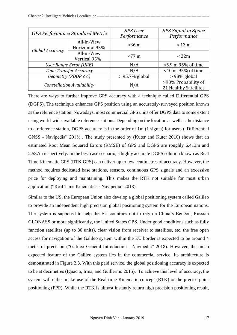
There are ways to further improve GPS accuracy with a technique called Differential GPS
(DGPS). The technique enhances GPS position using an accurately-surveyed position known
as the reference station. Nowadays, most commercial GPS units offer DGPS data to some extent
using world-wide available reference stations. Depending on the location as well as the distance
to a reference station, DGPS accuracy is in the order of 1m (1 sigma) for users (“Differential
GNSS - Navipedia” 2018) . The study presented by (Kuter and Kuter 2010) shows that an
estimated Root Mean Squared Errors (RMSE) of GPS and DGPS are roughly 6.413m and
2.587m respectively. In the best case scenario, a highly accurate DGPS solution known as Real
Time Kinematic GPS (RTK GPS) can deliver up to few centimetres of accuracy. However, the
method requires dedicated base stations, sensors, continuous GPS signals and an excessive
price for deploying and maintaining. This makes the RTK not suitable for most urban
application (“Real Time Kinematics - Navipedia” 2018).
Similar to the US, the European Union also develop a global positioning system called Galileo
to provide an independent high precision global positioning system for the European nations.
The system is supposed to help the EU countries not to rely on China’s BeiDou, Russian
GLONASS or more significantly, the United States GPS. Under good conditions such as fully
function satellites (up to 30 units), clear vision from receiver to satellites, etc. the free open
access for navigation of the Galileo system within the EU border is expected to be around 4
meter of precision (“Galileo General Introduction - Navipedia” 2018). However, the much
expected feature of the Galileo system lies in the commercial service. Its architecture is
demonstrated in Figure 2.3. With this paid service, the global positioning accuracy is expected
to be at decimetres (Ignacio, Irma, and Guillermo 2015). To achieve this level of accuracy, the
system will either make use of the Real-time Kinematic concept (RTK) or the precise point
positioning (PPP). While the RTK is almost instantly return high precision positioning result,

Chapter 2: Intelligent Vehicles Localization ------------------------------------------------------------------------------------------
Nguyen Dinh Van - January 2019 18
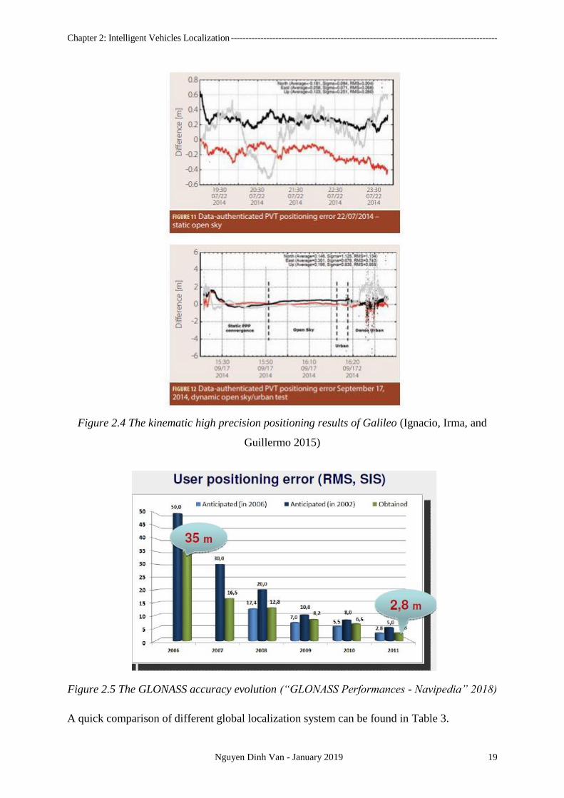
PPP requires 15-30 minutes of the initialization. Experiments results with the high precision
commercial positioning service are shown in Figure 2.4.
Figure 2.3 The Galileo satellites navigation system commercial service architecture
(Fernández-Hernández et al. 2018)
Another worth to mention global positioning system is the GLONASS developed by Russia in
1980s. By 2010, the GLONASS has covered the entire Russia territory then after October 2011,
the global coverage is achieved. The evolution of the GLONASS positioning accuracy is shown
in Figure 2.5. Up to now, under static sky, the GLONASS accuracy for public access is as good
as 2.8 meters.
Chapter 2: Intelligent Vehicles Localization ------------------------------------------------------------------------------------------
Nguyen Dinh Van - January 2019 19
Figure 2.4 The kinematic high precision positioning results of Galileo (Ignacio, Irma, and
Guillermo 2015)
Figure 2.5 The GLONASS accuracy evolution (“GLONASS Performances - Navipedia” 2018)
A quick comparison of different global localization system can be found in Table 3.
Chapter 2: Intelligent Vehicles Localization ------------------------------------------------------------------------------------------
Nguyen Dinh Van - January 2019 20
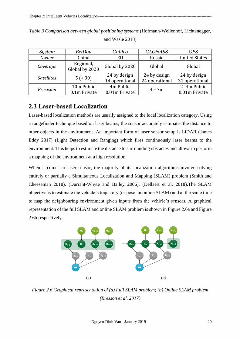
Table 3 Comparison between global positioning systems (Hofmann-Wellenhof, Lichtenegger,
and Wasle 2018)
System BeiDou Galileo GLONASS GPS
Owner China EU Russia United States
Coverage Regional,
Global by 2020 Global by 2020 Global Global
Satellites 5 (+ 30) 24 by design
14 operational 24 by design
24 operational 24 by design
31 operational
Precision 10m Public
0.1m Private 4m Public
0.01m Private 4 – 7m
2- 4m Public 0.01m Private
2.3 Laser-based Localization
Laser-based localization methods are usually assigned to the local localization category. Using
a rangefinder technique based on laser beams, the sensor accurately estimates the distance to
other objects in the environment. An important form of laser sensor setup is LiDAR (James
Eddy 2017) (Light Detection and Ranging) which fires continuously laser beams to the
environment. This helps to estimate the distance to surrounding obstacles and allows to perform
a mapping of the environment at a high resolution.
When it comes to laser sensor, the majority of its localization algorithms involve solving
entirely or partially a Simultaneous Localization and Mapping (SLAM) problem (Smith and
Cheeseman 2018), (Durrant-Whyte and Bailey 2006), (Dellaert et al. 2018).The SLAM
objective is to estimate the vehicle’s trajectory (or pose in online SLAM) and at the same time
to map the neighbouring environment given inputs from the vehicle’s sensors. A graphical
representation of the full SLAM and online SLAM problem is shown in Figure 2.6a and Figure
2.6b respectively.
Figure 2.6 Graphical representation of (a) Full SLAM problem; (b) Online SLAM problem
(Bresson et al. 2017)
Chapter 2: Intelligent Vehicles Localization ------------------------------------------------------------------------------------------
Nguyen Dinh Van - January 2019 21
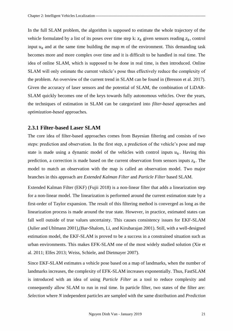
In the full SLAM problem, the algorithm is supposed to estimate the whole trajectory of the
vehicle formulated by a list of its poses over time step k: 𝑥𝑘 given sensors reading 𝑧𝑘, control
input 𝑢𝑘 and at the same time building the map 𝑚 of the environment. This demanding task
becomes more and more complex over time and it is difficult to be handled in real time. The
idea of online SLAM, which is supposed to be done in real time, is then introduced. Online
SLAM will only estimate the current vehicle’s pose thus effectively reduce the complexity of
the problem. An overview of the current trend in SLAM can be found in (Bresson et al. 2017).
Given the accuracy of laser sensors and the potential of SLAM, the combination of LiDAR-
SLAM quickly becomes one of the keys towards fully autonomous vehicles. Over the years,
the techniques of estimation in SLAM can be categorized into filter-based approaches and
optimization-based approaches.
2.3.1 Filter-based Laser SLAM
The core idea of filter-based approaches comes from Bayesian filtering and consists of two
steps: prediction and observation. In the first step, a prediction of the vehicle’s pose and map
state is made using a dynamic model of the vehicles with control inputs 𝑢𝑘 . Having this
prediction, a correction is made based on the current observation from sensors inputs 𝑧𝑘. The
model to match an observation with the map is called an observation model. Two major
branches in this approach are Extended Kalman Filter and Particle Filter based SLAM.
Extended Kalman Filter (EKF) (Fujii 2018) is a non-linear filter that adds a linearization step
for a non-linear model. The linearization is performed around the current estimation state by a
first-order of Taylor expansion. The result of this filtering method is converged as long as the
linearization process is made around the true state. However, in practice, estimated states can
fall well outside of true values uncertainty. This causes consistency issues for EKF-SLAM
(Julier and Uhlmann 2001),(Bar-Shalom, Li, and Kirubarajan 2001). Still, with a well-designed
estimation model, the EKF-SLAM is proved to be a success in a constrained situation such as
urban environments. This makes EFK-SLAM one of the most widely studied solution (Xie et
al. 2011; Elfes 2013; Weiss, Schiele, and Dietmayer 2007).
Since EKF-SLAM estimates a vehicle pose based on a map of landmarks, when the number of
landmarks increases, the complexity of EFK-SLAM increases exponentially. Thus, FastSLAM
is introduced with an idea of using Particle Filter as a tool to reduce complexity and
consequently allow SLAM to run in real time. In particle filter, two states of the filter are:
Selection where N independent particles are sampled with the same distribution and Prediction
Chapter 2: Intelligent Vehicles Localization ------------------------------------------------------------------------------------------
Nguyen Dinh Van - January 2019 22
where with each particle, a likelihood function is calculated as the score of how likely this
particle is the true state. Thus, by limiting the solution space within N particles, the complexity
of Particle Filter (PF) SLAM is then Ο(Nlog 𝐿) where L is number of landmarks in the map. In
contrast, the complexity of EKF-SLAM is Ο(𝐿2). When the number of landmarks increases,
the advantage of PF-SLAM becomes more and more significant. Works in (Hahnel et al. 2018;
Mohan and MadhavaKrishna 2010; Montemerlo et al. 2018) demonstrates FastSLAM approach
which can work in a large scale environment and (Reineking and Clemens 2013; Trehard et al.
2014) implements FastSLAM using evidential theory instead of a classical probabilistic model.
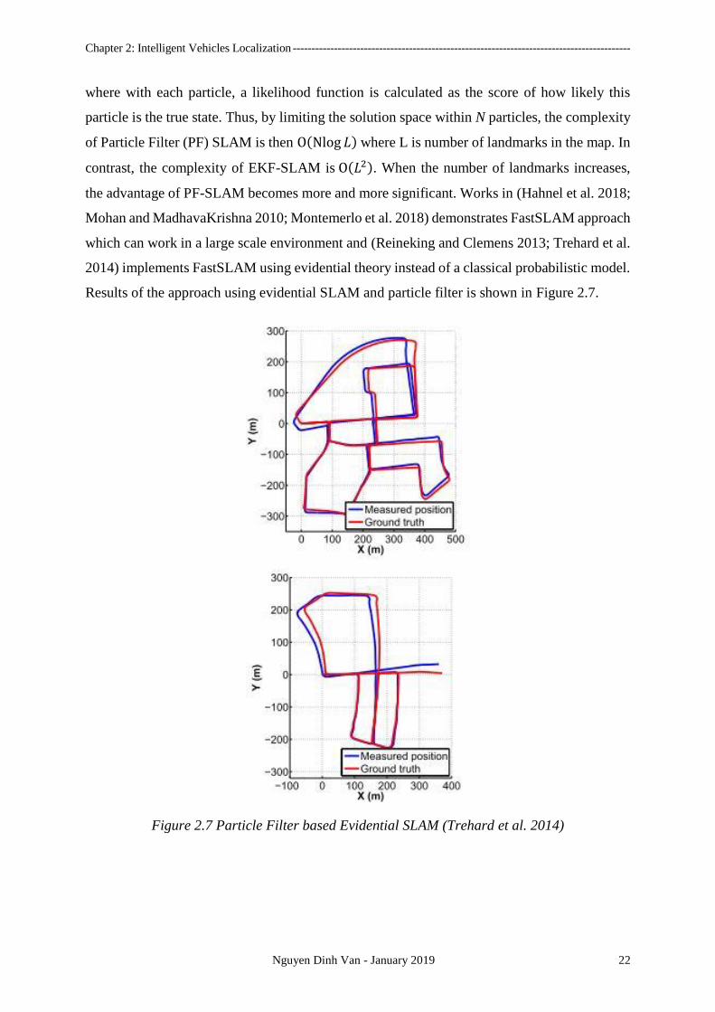
Results of the approach using evidential SLAM and particle filter is shown in Figure 2.7.
Figure 2.7 Particle Filter based Evidential SLAM (Trehard et al. 2014)
Chapter 2: Intelligent Vehicles Localization ------------------------------------------------------------------------------------------
Nguyen Dinh Van - January 2019 23
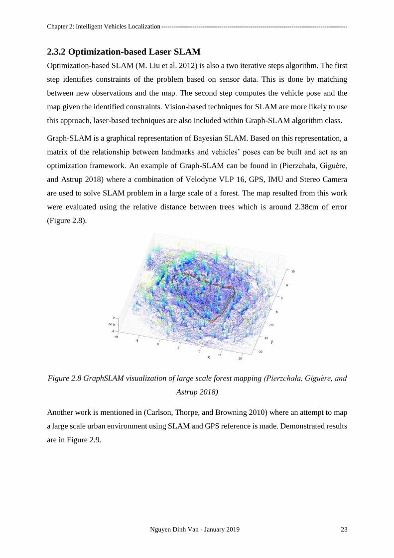
2.3.2 Optimization-based Laser SLAM
Optimization-based SLAM (M. Liu et al. 2012) is also a two iterative steps algorithm. The first
step identifies constraints of the problem based on sensor data. This is done by matching
between new observations and the map. The second step computes the vehicle pose and the
map given the identified constraints. Vision-based techniques for SLAM are more likely to use
this approach, laser-based techniques are also included within Graph-SLAM algorithm class.
Graph-SLAM is a graphical representation of Bayesian SLAM. Based on this representation, a
matrix of the relationship between landmarks and vehicles’ poses can be built and act as an
optimization framework. An example of Graph-SLAM can be found in (Pierzchała, Giguère,
and Astrup 2018) where a combination of Velodyne VLP 16, GPS, IMU and Stereo Camera
are used to solve SLAM problem in a large scale of a forest. The map resulted from this work
were evaluated using the relative distance between trees which is around 2.38cm of error
(Figure 2.8).
Figure 2.8 GraphSLAM visualization of large scale forest mapping (Pierzchała, Giguère, and
Astrup 2018)
Another work is mentioned in (Carlson, Thorpe, and Browning 2010) where an attempt to map
a large scale urban environment using SLAM and GPS reference is made. Demonstrated results
are in Figure 2.9.
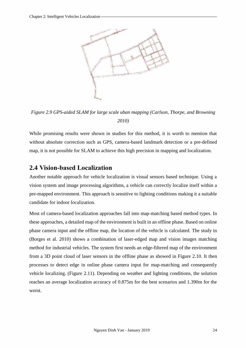
Chapter 2: Intelligent Vehicles Localization ------------------------------------------------------------------------------------------
Nguyen Dinh Van - January 2019 24
Figure 2.9 GPS-aided SLAM for large scale uban mapping (Carlson, Thorpe, and Browning
2010)
While promising results were shown in studies for this method, it is worth to mention that
without absolute correction such as GPS, camera-based landmark detection or a pre-defined
map, it is not possible for SLAM to achieve this high precision in mapping and localization.
2.4 Vision-based Localization
Another notable approach for vehicle localization is visual sensors based technique. Using a
vision system and image processing algorithms, a vehicle can correctly localize itself within a
pre-mapped environment. This approach is sensitive to lighting conditions making it a suitable
candidate for indoor localization.
Most of camera-based localization approaches fall into map-matching based method types. In
these approaches, a detailed map of the environment is built in an offline phase. Based on online
phase camera input and the offline map, the location of the vehicle is calculated. The study in
(Borges et al. 2010) shows a combination of laser-edged map and vision images matching
method for industrial vehicles. The system first needs an edge-filtered map of the environment
from a 3D point cloud of laser sensors in the offline phase as showed in Figure 2.10. It then
processes to detect edge in online phase camera input for map-matching and consequently
vehicle localizing. (Figure 2.11). Depending on weather and lighting conditions, the solution
reaches an average localization accuracy of 0.875m for the best scenarios and 1.390m for the
worst.

Chapter 2: Intelligent Vehicles Localization ------------------------------------------------------------------------------------------
Nguyen Dinh Van - January 2019 25
Figure 2.10 Edge-filtered map of the environment (Borges et al. 2010)
Figure 2.11 Camera image to edge image transformation (Borges et al. 2010)
Similar to Laser SLAM, visual SLAM is a popular approach for intelligent vehicles
localization. The SLAM concept remains the same as in the laser SLAM but in this case a set
of cameras is mounted on the vehicle to capture not only images but also to measure the depth
of the scene. An interesting research work proposed by (Shi et al. 2012) consists of a fusion of
GPS and aided visual SLAM methods, which does not use any additional sensor. The system
however consists of six calibrated fish eyes cameras with a dual-frequency GPS receiver. In an
offline mapping phase, the GPS observation is supported by CORS RTK technology which has
an accuracy within 0.02m. Based on this map, the online localization method yields an accurate
position with an average error under 0.067m. Note that this paper uses only 8 checkpoints as
an evaluation ground truth and no lighting condition is mentioned.
2.5 Dead-Reckoning
Dead-reckoning is a process of estimating the current pose of a vehicle using a previously
determined pose and the vehicle’s dynamic model. Initially, it was an approach developed for

Chapter 2: Intelligent Vehicles Localization ------------------------------------------------------------------------------------------
Nguyen Dinh Van - January 2019 26
marine applications and has now been used in a variety of fields such as air navigation,
pedestrian tracking or autonomous robot navigation.
The dead-reckoning algorithm makes use of different sensor configurations. Dead-reckoning
with Inertial Measurement Units (IMU) is widely used in the navigation of spacecraft, marine
ships or landline vehicles. IMU typically has three-axis gyroscopes and accelerators to measure
angular and displacement velocity of the attached object.
Depending on the precision of sensors inside the IMU (gyroscopes and accelerators), the dead-
reckoning can incrementally estimate the local pose of the vehicle using a pre-defined dynamic
model. This, however, results in the accumulated error over time as inaccuracy in each
measurement adds up. It is almost impossible to correct this error by the system itself as there
is no absolute reference source. An attempt to fix this problem using dual drive system and
modelling of expected accumulated error is found in (Borenstein 1995), yet the result is limited.
Consequently, almost all dead-reckoning solutions are now used in fusion with other
localization techniques such as GPS (Fouque et al. 2008), laser-SLAM (Akai et al. 2017) or
vision-based (Vivacqua et al. 2018). The idea is to incorporate an absolute reference to regularly
correct the accumulated error results from the dead-reckoning process. An example of a solution
to correct dead-reckoning using static map can be found in (Fouque et al. 2008). The result of
this solution is shown in Figure 2.12. It can be seen in the figure that even with correction from
static map and some GPS injection, the dead-reckoning still has a large accumulated error over
time (around 22m).
In conclusion, the general accuracy estimation of this method is large. It heavily depends on the
precision of IMU components, the dynamic model of the vehicle as well as any possible
correction applied. A carefully designed dead-reckoning process using high precision sensors
could be extremely accurate in a close range. This makes dead-reckoning a preferable solution
for indoor localization (Z. Liu et al. 2017; Huijie Chen, Li, and Wang 2018).

Chapter 2: Intelligent Vehicles Localization ------------------------------------------------------------------------------------------
Nguyen Dinh Van - January 2019 27
Figure 2.12 Dead-reckoning and static map (Fouque et al. 2008)
2.6 Intelligent Vehicles Localization in GPS-denied Environments
One of the drawbacks of GPS is its availability in urban scenarios. More often, GPS signals are
lost or poorly received in a tunnel, a carpark or when the receiver is surrounded by buildings
thus obstructs line-of-sight to satellites. The standard GPS signals also suffer from the multi-
path effect which could result in additional 8m of error in localization (Kos, Markezic, and
Pokrajcic 2010). Still, GPS (and other GNSSs) plays a vital role in localization especially at the
global scale as it is the only positioning system that directly outputs in the global coordinate
frame. Without this global reference coordinates, each intelligent vehicle will work on its own
local coordinates hence no communication or cooperation is possible.
In the last few years, the research community in Intelligent Vehicles has been developing
several dedicated systems for localization in GPS-denied areas in general and carparks in
particular. Due to the lack of GPS signals, most of the solutions for localization in this domain
fall into the local localization level. Depending on the choice of the reference coordinate system,
these works can be categorized into two classes: absolute localization (or map-based) methods
and relative localization (self-centric, without a map) methods. The two classes’ recent works
will be studied in the following sections.
2.6.1 Absolute Localization
In the absolute positioning approach, it is required that a map of the environment is known
beforehand by the vehicle. In this map, there are two main components: static objects which
contribute to the structure of the map (e.g. road, walls, doors, etc.), and dynamic objects which
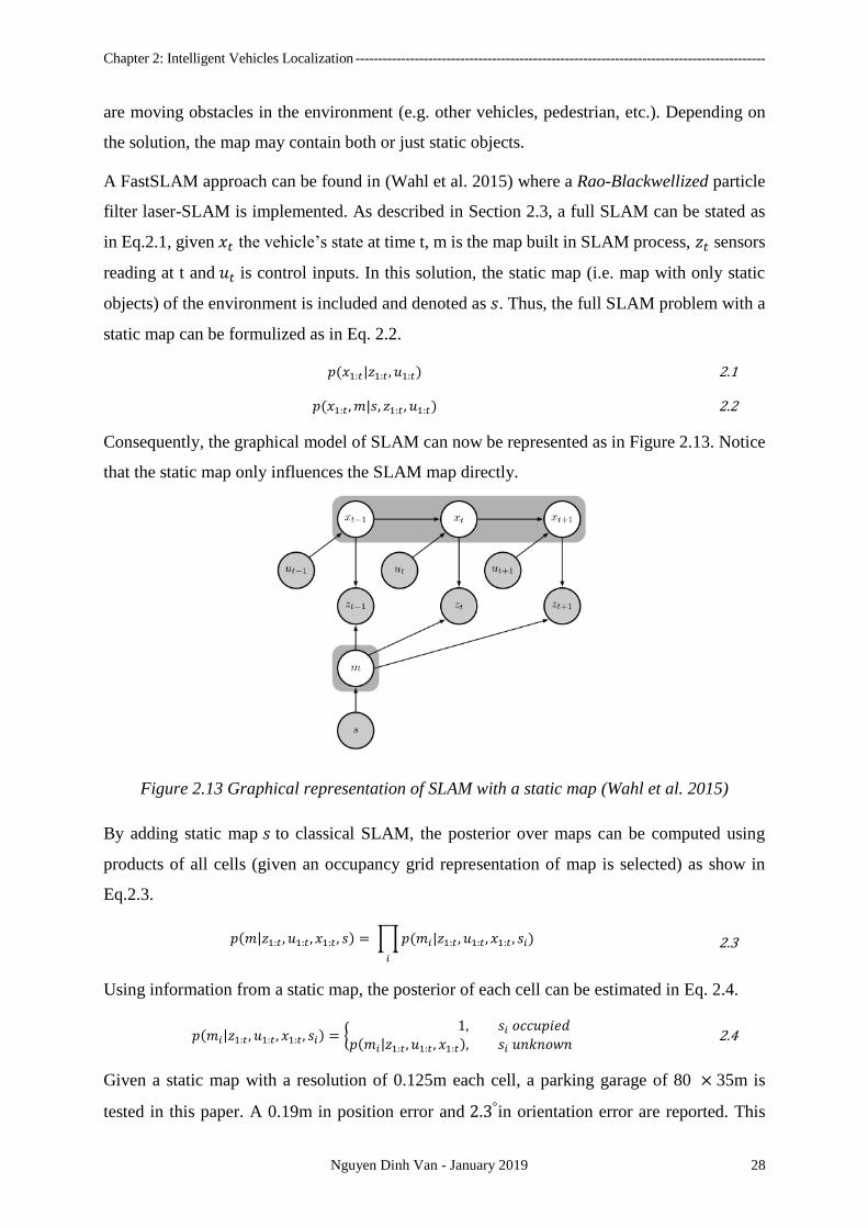
Chapter 2: Intelligent Vehicles Localization ------------------------------------------------------------------------------------------
Nguyen Dinh Van - January 2019 28
are moving obstacles in the environment (e.g. other vehicles, pedestrian, etc.). Depending on
the solution, the map may contain both or just static objects.
A FastSLAM approach can be found in (Wahl et al. 2015) where a Rao-Blackwellized particle
filter laser-SLAM is implemented. As described in Section 2.3, a full SLAM can be stated as
in Eq.2.1, given 𝑥𝑡 the vehicle’s state at time t, m is the map built in SLAM process, 𝑧𝑡 sensors
reading at t and 𝑢𝑡 is control inputs. In this solution, the static map (i.e. map with only static
objects) of the environment is included and denoted as 𝑠. Thus, the full SLAM problem with a
static map can be formulized as in Eq. 2.2.
𝑝(𝑥1:𝑡|𝑧1:𝑡 , 𝑢1:𝑡) 2.1
𝑝(𝑥1:𝑡 , 𝑚|𝑠, 𝑧1:𝑡 , 𝑢1:𝑡) 2.2
Consequently, the graphical model of SLAM can now be represented as in Figure 2.13. Notice
that the static map only influences the SLAM map directly.
Figure 2.13 Graphical representation of SLAM with a static map (Wahl et al. 2015)
By adding static map 𝑠 to classical SLAM, the posterior over maps can be computed using
products of all cells (given an occupancy grid representation of map is selected) as show in
Eq.2.3.
𝑝(𝑚|𝑧1:𝑡 , 𝑢1:𝑡 , 𝑥1:𝑡 , 𝑠) = ∏𝑝(𝑚𝑖|𝑧1:𝑡 , 𝑢1:𝑡 , 𝑥1:𝑡 , 𝑠𝑖)
𝑖
2.3
Using information from a static map, the posterior of each cell can be estimated in Eq. 2.4.
𝑝(𝑚𝑖|𝑧1:𝑡 , 𝑢1:𝑡 , 𝑥1:𝑡 , 𝑠𝑖) = 1, 𝑠𝑖 𝑜𝑐𝑐𝑢𝑝𝑖𝑒𝑑
𝑝(𝑚𝑖|𝑧1:𝑡 , 𝑢1:𝑡 , 𝑥1:𝑡), 𝑠𝑖 𝑢𝑛𝑘𝑛𝑜𝑤𝑛 2.4
Given a static map with a resolution of 0.125m each cell, a parking garage of 80 × 35m is
tested in this paper. A 0.19m in position error and 2.3°in orientation error are reported. This
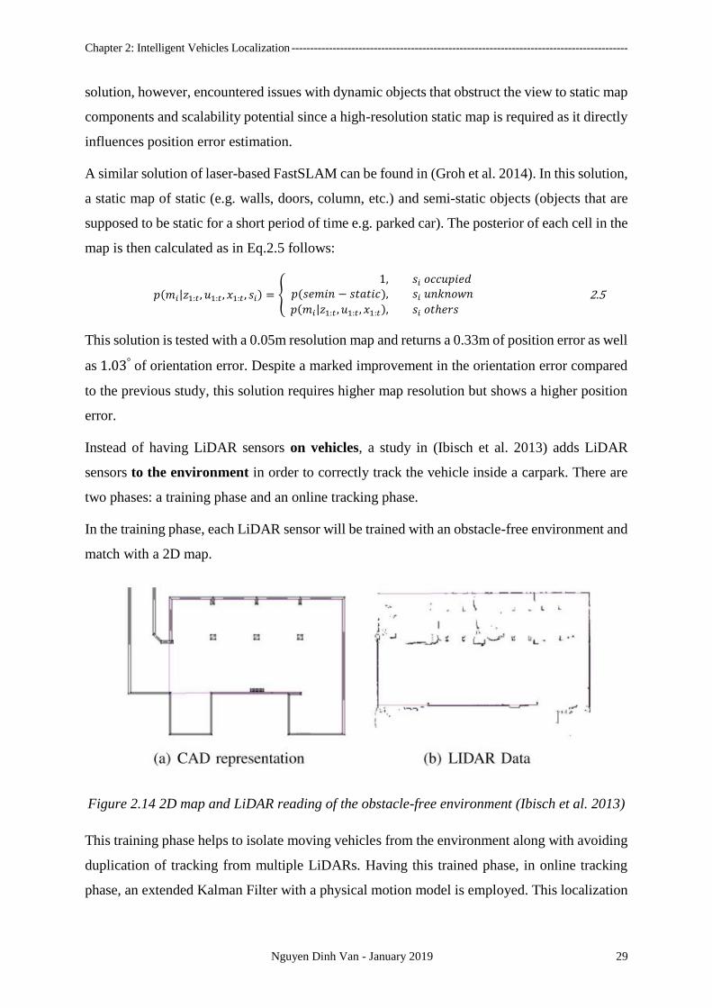
Chapter 2: Intelligent Vehicles Localization ------------------------------------------------------------------------------------------
Nguyen Dinh Van - January 2019 29
solution, however, encountered issues with dynamic objects that obstruct the view to static map
components and scalability potential since a high-resolution static map is required as it directly
influences position error estimation.
A similar solution of laser-based FastSLAM can be found in (Groh et al. 2014). In this solution,
a static map of static (e.g. walls, doors, column, etc.) and semi-static objects (objects that are
supposed to be static for a short period of time e.g. parked car). The posterior of each cell in the
map is then calculated as in Eq.2.5 follows:
𝑝(𝑚𝑖|𝑧1:𝑡 , 𝑢1:𝑡 , 𝑥1:𝑡 , 𝑠𝑖) =
1, 𝑠𝑖 𝑜𝑐𝑐𝑢𝑝𝑖𝑒𝑑𝑝(𝑠𝑒𝑚𝑖𝑛 − 𝑠𝑡𝑎𝑡𝑖𝑐), 𝑠𝑖 𝑢𝑛𝑘𝑛𝑜𝑤𝑛
𝑝(𝑚𝑖|𝑧1:𝑡 , 𝑢1:𝑡 , 𝑥1:𝑡), 𝑠𝑖 𝑜𝑡ℎ𝑒𝑟𝑠 2.5
This solution is tested with a 0.05m resolution map and returns a 0.33m of position error as well
as 1.03° of orientation error. Despite a marked improvement in the orientation error compared
to the previous study, this solution requires higher map resolution but shows a higher position
error.
Instead of having LiDAR sensors on vehicles, a study in (Ibisch et al. 2013) adds LiDAR
sensors to the environment in order to correctly track the vehicle inside a carpark. There are
two phases: a training phase and an online tracking phase.
In the training phase, each LiDAR sensor will be trained with an obstacle-free environment and
match with a 2D map.
Figure 2.14 2D map and LiDAR reading of the obstacle-free environment (Ibisch et al. 2013)
This training phase helps to isolate moving vehicles from the environment along with avoiding
duplication of tracking from multiple LiDARs. Having this trained phase, in online tracking
phase, an extended Kalman Filter with a physical motion model is employed. This localization
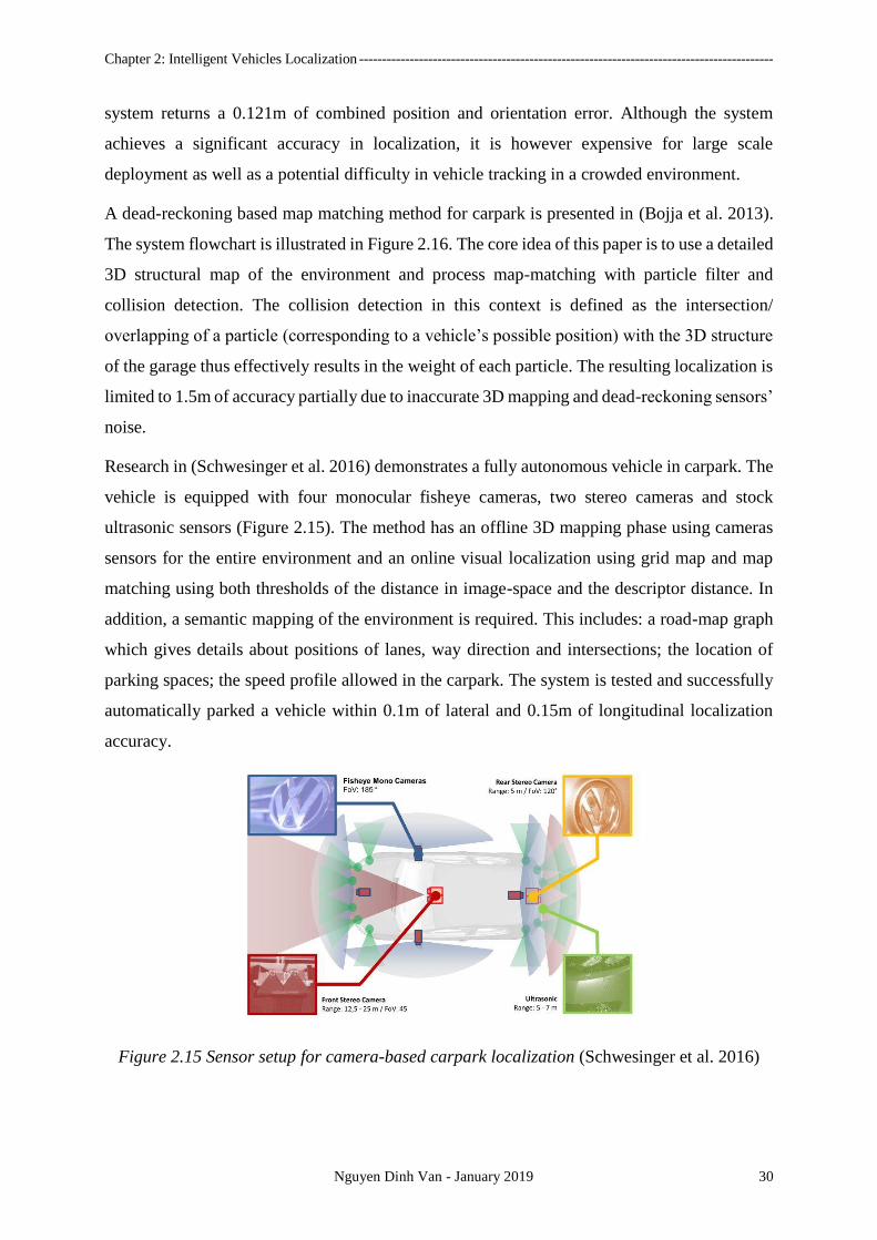
Chapter 2: Intelligent Vehicles Localization ------------------------------------------------------------------------------------------
Nguyen Dinh Van - January 2019 30
system returns a 0.121m of combined position and orientation error. Although the system
achieves a significant accuracy in localization, it is however expensive for large scale
deployment as well as a potential difficulty in vehicle tracking in a crowded environment.
A dead-reckoning based map matching method for carpark is presented in (Bojja et al. 2013).
The system flowchart is illustrated in Figure 2.16. The core idea of this paper is to use a detailed
3D structural map of the environment and process map-matching with particle filter and
collision detection. The collision detection in this context is defined as the intersection/
overlapping of a particle (corresponding to a vehicle’s possible position) with the 3D structure
of the garage thus effectively results in the weight of each particle. The resulting localization is
limited to 1.5m of accuracy partially due to inaccurate 3D mapping and dead-reckoning sensors’
noise.
Research in (Schwesinger et al. 2016) demonstrates a fully autonomous vehicle in carpark. The
vehicle is equipped with four monocular fisheye cameras, two stereo cameras and stock
ultrasonic sensors (Figure 2.15). The method has an offline 3D mapping phase using cameras
sensors for the entire environment and an online visual localization using grid map and map
matching using both thresholds of the distance in image-space and the descriptor distance. In
addition, a semantic mapping of the environment is required. This includes: a road-map graph
which gives details about positions of lanes, way direction and intersections; the location of
parking spaces; the speed profile allowed in the carpark. The system is tested and successfully
automatically parked a vehicle within 0.1m of lateral and 0.15m of longitudinal localization
accuracy.
Figure 2.15 Sensor setup for camera-based carpark localization (Schwesinger et al. 2016)
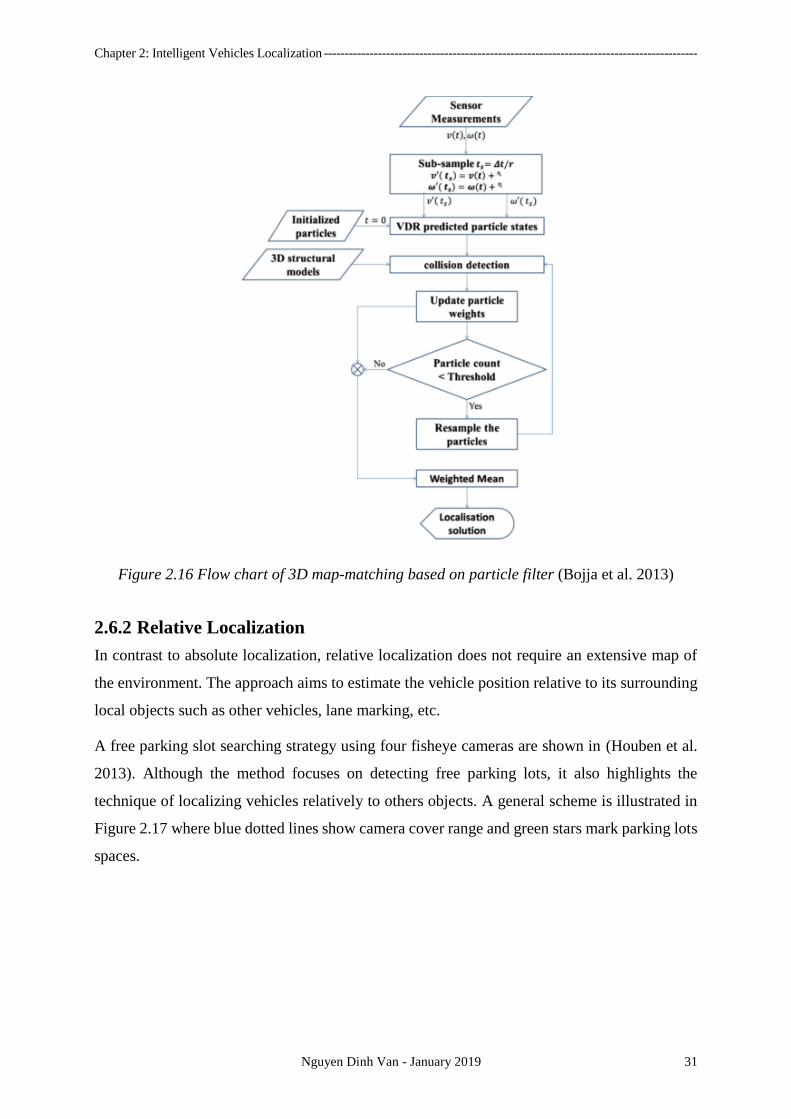
Chapter 2: Intelligent Vehicles Localization ------------------------------------------------------------------------------------------
Nguyen Dinh Van - January 2019 31
Figure 2.16 Flow chart of 3D map-matching based on particle filter (Bojja et al. 2013)
2.6.2 Relative Localization
In contrast to absolute localization, relative localization does not require an extensive map of
the environment. The approach aims to estimate the vehicle position relative to its surrounding
local objects such as other vehicles, lane marking, etc.
A free parking slot searching strategy using four fisheye cameras are shown in (Houben et al.
2013). Although the method focuses on detecting free parking lots, it also highlights the
technique of localizing vehicles relatively to others objects. A general scheme is illustrated in
Figure 2.17 where blue dotted lines show camera cover range and green stars mark parking lots
spaces.
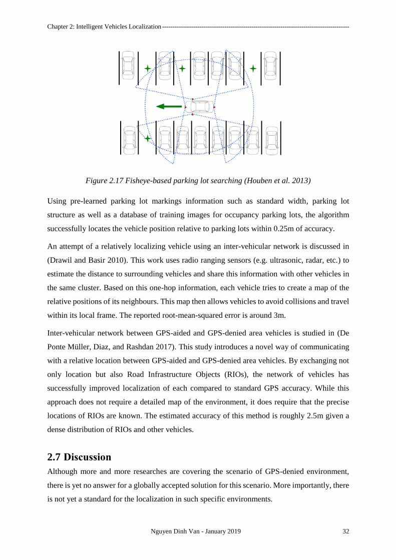
Chapter 2: Intelligent Vehicles Localization ------------------------------------------------------------------------------------------
Nguyen Dinh Van - January 2019 32
Figure 2.17 Fisheye-based parking lot searching (Houben et al. 2013)
Using pre-learned parking lot markings information such as standard width, parking lot
structure as well as a database of training images for occupancy parking lots, the algorithm
successfully locates the vehicle position relative to parking lots within 0.25m of accuracy.
An attempt of a relatively localizing vehicle using an inter-vehicular network is discussed in
(Drawil and Basir 2010). This work uses radio ranging sensors (e.g. ultrasonic, radar, etc.) to
estimate the distance to surrounding vehicles and share this information with other vehicles in
the same cluster. Based on this one-hop information, each vehicle tries to create a map of the
relative positions of its neighbours. This map then allows vehicles to avoid collisions and travel
within its local frame. The reported root-mean-squared error is around 3m.
Inter-vehicular network between GPS-aided and GPS-denied area vehicles is studied in (De
Ponte Müller, Diaz, and Rashdan 2017). This study introduces a novel way of communicating
with a relative location between GPS-aided and GPS-denied area vehicles. By exchanging not
only location but also Road Infrastructure Objects (RIOs), the network of vehicles has
successfully improved localization of each compared to standard GPS accuracy. While this
approach does not require a detailed map of the environment, it does require that the precise
locations of RIOs are known. The estimated accuracy of this method is roughly 2.5m given a
dense distribution of RIOs and other vehicles.
2.7 Discussion
Although more and more researches are covering the scenario of GPS-denied environment,
there is yet no answer for a globally accepted solution for this scenario. More importantly, there
is not yet a standard for the localization in such specific environments.
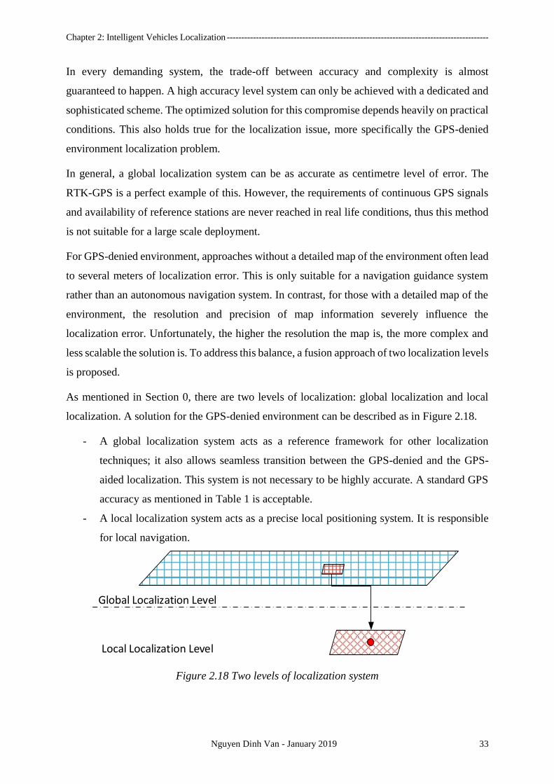
Chapter 2: Intelligent Vehicles Localization ------------------------------------------------------------------------------------------
Nguyen Dinh Van - January 2019 33
In every demanding system, the trade-off between accuracy and complexity is almost
guaranteed to happen. A high accuracy level system can only be achieved with a dedicated and
sophisticated scheme. The optimized solution for this compromise depends heavily on practical
conditions. This also holds true for the localization issue, more specifically the GPS-denied
environment localization problem.
In general, a global localization system can be as accurate as centimetre level of error. The
RTK-GPS is a perfect example of this. However, the requirements of continuous GPS signals
and availability of reference stations are never reached in real life conditions, thus this method
is not suitable for a large scale deployment.
For GPS-denied environment, approaches without a detailed map of the environment often lead
to several meters of localization error. This is only suitable for a navigation guidance system
rather than an autonomous navigation system. In contrast, for those with a detailed map of the
environment, the resolution and precision of map information severely influence the
localization error. Unfortunately, the higher the resolution the map is, the more complex and
less scalable the solution is. To address this balance, a fusion approach of two localization levels
is proposed.
As mentioned in Section 0, there are two levels of localization: global localization and local
localization. A solution for the GPS-denied environment can be described as in Figure 2.18.
- A global localization system acts as a reference framework for other localization
techniques; it also allows seamless transition between the GPS-denied and the GPS-
aided localization. This system is not necessary to be highly accurate. A standard GPS
accuracy as mentioned in Table 1 is acceptable.
- A local localization system acts as a precise local positioning system. It is responsible
for local navigation.
Global Localization Level
Local Localization Level
Figure 2.18 Two levels of localization system

Chapter 2: Intelligent Vehicles Localization ------------------------------------------------------------------------------------------
Nguyen Dinh Van - January 2019 34
The advantages of this approach are its scalability and accuracy characteristics. Each level of
localization has a reasonable expectation of accuracy (low accuracy in broad view and high
accuracy in local view). Also the existence of both level allows the system to scale and work
seamlessly with other existed localization systems. Even though the complexity level of this
fusion approach is not entirely reduced, the two levels fusion system is relatively straight
forward and provides an opportunity of reducing global map resolution.

Chapter 2: Intelligent Vehicles Localization ------------------------------------------------------------------------------------------
Nguyen Dinh Van - January 2019 35

36
3. WIRELESS SENSOR NETWORKS LOCALIZATION
Résumé
Les réseaux de capteurs sans fil (WSN) font référence à un groupe de capteurs dispersés et
dédiés dans l’espace pour surveiller et enregistrer les conditions physiques de l’environnement
et organiser les données collectées à un emplacement central. Le GNSS, qui est une partie
cruciale de ITS, est un exemple parfait de WSN pour des applications ITS. Le GNSS en général
ou le GPS en particulier ont établi une norme pour le système de navigation global des véhicules
intelligents. Malgré ses faiblesses dans les zones obstruées, l'impact du GPS est toujours
important. En outre, le concept de localisation dans le GPS suggère une application possible
des réseaux à grande vitesse (WSN) pour couvrir également ces zones obstruées. Ce chapitre
examinera la stratégie de localisation des véhicules intelligents en particulier des réseaux
intelligents WSN.
Il existe différents types de capteurs sans fil ainsi que des formes de réseaux pour les tâches de
localisation à l'aide de WSN. Les capteurs sont infrarouges, ultrasoniques, unités de mesure
inertielle (IMU), antenne Wi-Fi, etc. Les exemples de réseaux peuvent être le réseau satellite
de GPS, le réseau cellulaire GSM, les réseaux Wi-Fi ou des réseaux plus spécifiques tels que
Zigbee ou Bluetooth. Malgré les différences de types de capteurs et de formes de réseaux, les
stratégies de localisation à l'aide de WSN peuvent être classées en deux classes: approches
basées sur les gammes et approches sans plages.
Les approches basées sur la distance pour la localisation des WSN sont un groupe de méthodes
qui estiment l'emplacement de l'objet d'intérêt en fonction de mesures de distance déduites des
sorties de capteurs sans fil. Ces approches comportent deux étapes: les mesures de distance et
l’estimation de la position. Souvent, des capteurs dotés de fonctions de mesure de distance telles
Chapter 3: Wireless Sensor Networks Localization ---------------------------------------------------------------------------------
Nguyen Dinh Van - January 2019 37
que les ultrasons, les UMI, les lasers, etc. peuvent directement être utilisés pour déduire la
distance entre des objets d’intérêt et d’autres objets de l’environnement et permettre ainsi une
estimation de la localisation possible. Cependant, il existe d’autres capteurs qui peuvent déduire
indirectement la distance aux IO, tels que les signaux satellites, les signaux cellulaires, les
signaux Wi-Fi, etc. ), Algorithme Heure d'arrivée (TOA), décalage horaire (TDOA), ou angle
d'arrivée (AOA), etc.
En revanche, les approches par fourchette de frais n’estiment pas la distance entre les OI et les
OOI pour calculer la position. Ces méthodes utilisent des fonctionnalités de réseau et de
capteurs telles que le graphe de connectivité réseau, la consommation d'énergie des capteurs et
leur transmission ou la relation géométrique d'un réseau, etc. La plupart du temps, ces approches
comportent deux étapes: l'extraction de caractéristiques et la reconnaissance de caractéristiques.
Les algorithmes remarquables pour cette classe sont le saut de vecteur de distance (DV hop), le
test de point approximatif de triangulation (APIT), l’empreinte digitale et l’algorithme de
centroïde.
Le tableau 4 présente une comparaison rapide de ces approches.
3.1 Introduction
Wireless Sensors Networks (WSNs) refer to a group of spatially dispersed and dedicated
sensors for monitoring and recording the physical conditions of the environment and organizing
the collected data at a central location (“Wireless Sensors Networks” 2018). Before the era of
the Internet of Things (IoT) wireless sensors networks have already been used in a variety of
scenarios such as: weather monitoring system, disaster prevention, localization and tracking,
etc. As devices become cheaper and smaller, the application domain of WSNs spreads wider.
One of which concerns Intelligent Transportation System (ITS).
The GNSS, which is a crucial part of ITS, is a perfect example of WSNs for ITS applications.
The GNSS in general or GPS in particular has set a standard for the global navigation system
of intelligent vehicles. Despite its weaknesses in obstructed areas, the impact of GPS is still
large. In addition, the concept of localization in GPS suggests a possible application of WSNs
to cover those obstructed areas as well. This chapter will take a look at WSNs strategy for
localization in general and intelligent vehicles localization in particular.
Chapter 3: Wireless Sensor Networks Localization ---------------------------------------------------------------------------------
Nguyen Dinh Van - January 2019 38
3.2 Localization Strategies Overview
There are various types of wireless sensors as well as forms of networks for localization task
using WSNs. The sensors are infrared, ultrasonic, Inertial Measurement Units (IMU), Wi-Fi
antenna, etc. and Networks examples could be the Satellites network of GPS, the GSM cellular
network, Wi-Fi networks or more specific networks such as Zigbee, or Bluetooth. Despite
differences in sensors types and networks forms, the strategies of localization using WSNs can
be categorized into two classes: Range-based and Range-free approaches.
Range-based approaches for WSNs localization are a group of methods that estimate the
location of the object of interest based on distance measurements inferred from wireless sensors
outputs. These approaches have two stages: distance measurements and position estimation.
Often, sensors with distance measuring feature such as ultrasonic, IMU, lasers, etc. which can
directly be used to infer the distance from/to objects of interest (OOIs) to other objects in the
environment and thus possible location estimation can be calculated. However, there are other
sensors that can indirectly infer the distance to OOIs such as Satellites signals, cellular signals,
Wi-Fi signals, etc. The distance computation from these sensors outputs is based on a signal
propagation model using Received Signal Strength Indicator (RSSI), Time of Arrival (TOA),
Time Difference of Arrival (TDOA), or Angle of Arrival (AOA) algorithm, etc.
Range-fee approaches, in contrary, do not estimate the distance to/from OOIs in order to
calculate position. Those methods use network and sensors features such as network
connectivity graph, sensors power consumption and transmission or geometric relationship of
network etc. Most of the time, these approaches have two steps: feature extractions and feature
recognition. Notable algorithms for this class are distance vector hop (DV hop), approximate
point-in-triangulation test (APIT), fingerprinting and centroid algorithm.
3.3 Range-based Approach
3.3.1 Time of Arrival
Time of arrival (TOA) refers to the time for radio signal travel from the transmitter to a receiver.
It is sometimes called Time of Flight. One of the first studies of this method is mentioned in
(Caffery 2000). Due to the known constant speed of radio signal in the air, the distance between
two nodes (transmitter and receiver) can be calculated if the time for radio signal to travel is
also known. There are two schemes for measuring this elapsed time: one-way scheme and two-
way scheme.
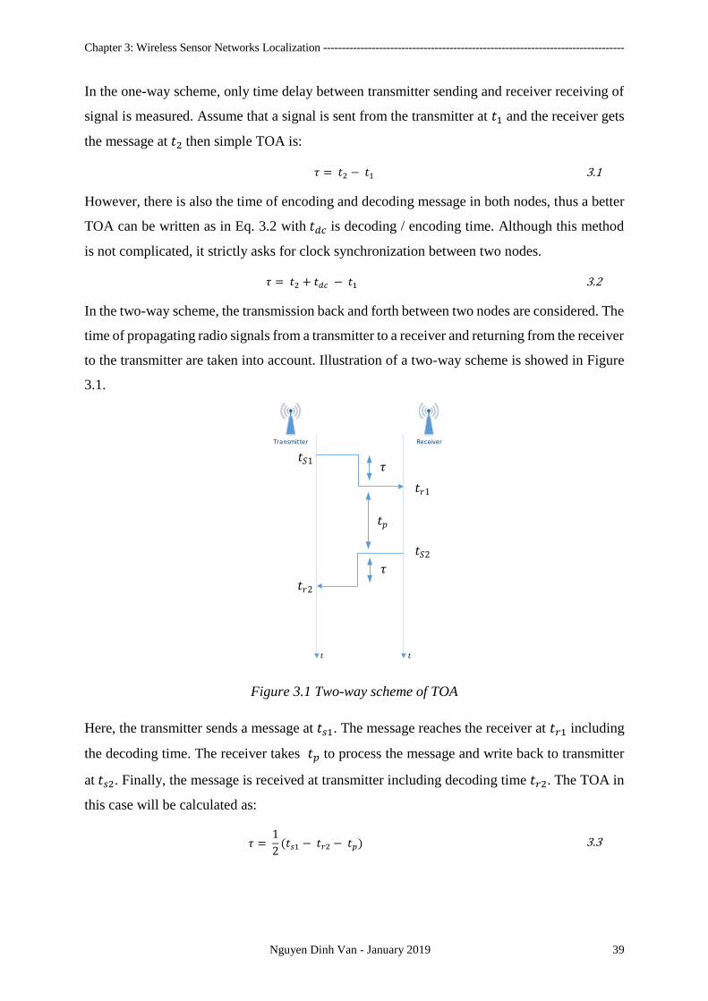
Chapter 3: Wireless Sensor Networks Localization ---------------------------------------------------------------------------------
Nguyen Dinh Van - January 2019 39
In the one-way scheme, only time delay between transmitter sending and receiver receiving of
signal is measured. Assume that a signal is sent from the transmitter at 𝑡1 and the receiver gets
the message at 𝑡2 then simple TOA is:
𝜏 = 𝑡2 − 𝑡1 3.1
However, there is also the time of encoding and decoding message in both nodes, thus a better
TOA can be written as in Eq. 3.2 with 𝑡𝑑𝑐 is decoding / encoding time. Although this method
is not complicated, it strictly asks for clock synchronization between two nodes.
𝜏 = 𝑡2 + 𝑡𝑑𝑐 − 𝑡1 3.2
In the two-way scheme, the transmission back and forth between two nodes are considered. The
time of propagating radio signals from a transmitter to a receiver and returning from the receiver
to the transmitter are taken into account. Illustration of a two-way scheme is showed in Figure
3.1.
Transmitter Receiver
𝑡𝑆1
𝑡𝑟1
𝑡𝑆2
𝑡𝑟2
𝑡𝑝
𝑡 𝑡
𝜏
𝜏
Figure 3.1 Two-way scheme of TOA
Here, the transmitter sends a message at 𝑡𝑠1. The message reaches the receiver at 𝑡𝑟1 including
the decoding time. The receiver takes 𝑡𝑝 to process the message and write back to transmitter
at 𝑡𝑠2. Finally, the message is received at transmitter including decoding time 𝑡𝑟2. The TOA in
this case will be calculated as:
𝜏 = 1
2(𝑡𝑠1 − 𝑡𝑟2 − 𝑡𝑝) 3.3
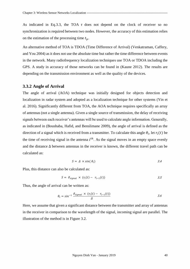
Chapter 3: Wireless Sensor Networks Localization ---------------------------------------------------------------------------------
Nguyen Dinh Van - January 2019 40
As indicated in Eq.3.3, the TOA 𝜏 does not depend on the clock of receiver so no
synchronization is required between two nodes. However, the accuracy of this estimation relies
on the estimation of the processing time 𝑡𝑝.
An alternative method of TOA is TDOA (Time Difference of Arrival) (Venkatraman, Caffery,
and You 2004) as it does not use the absolute time but rather the time difference between events
in the network. Many radiofrequency localization techniques use TOA or TDOA including the
GPS. A study in accuracy of those networks can be found in (Kaune 2012). The results are
depending on the transmission environment as well as the quality of the devices.
3.3.2 Angle of Arrival
The angle of arrival (AOA) technique was initially designed for objects detection and
localization in radar system and adopted as a localization technique for other systems (Yin et
al. 2016). Significantly different from TOA, the AOA technique requires specifically an array
of antennas (not a single antenna). Given a single source of transmission, the delay of receiving
signals between each receiver’s antennas will be used to calculate angle information. Generally,
as indicated in (Boushaba, Hafid, and Benslimane 2009), the angle of arrival is defined as the
direction of a signal which is received from a transmitter. To calculate this angle 𝜃𝑙, let 𝑟𝑖(𝑡) be
the time of receiving signal in the antenna 𝑖𝑡ℎ. As the signal moves in an empty space evenly
and the distance Δ between antennas in the receiver is known, the different travel path can be
calculated as:
𝑆 = 𝛥 × 𝑠𝑖𝑛( 𝜃𝑙) 3.4
Plus, this distance can also be calculated as:
𝑆 = 𝜗𝑠𝑖𝑔𝑛𝑎𝑙 × (𝑟𝑖(𝑡) − 𝑟𝑖−1(𝑡)) 3.5
Thus, the angle of arrival can be written as:
𝜃𝑙 = 𝑠𝑖𝑛−1 𝜗𝑠𝑖𝑔𝑛𝑎𝑙 × (𝑟𝑖(𝑡) − 𝑟𝑖−1(𝑡))
𝛥 3.6
Here, we assume that given a significant distance between the transmitter and array of antennas
in the receiver in comparison to the wavelength of the signal, incoming signal are parallel. The
illustration of the method is in Figure 3.2.

Chapter 3: Wireless Sensor Networks Localization ---------------------------------------------------------------------------------
Nguyen Dinh Van - January 2019 41
Figure 3.2 Angle of Arrival (AOA) localization method (Yin et al. 2016)
By calculating multiples AOA of different transmitters, the position of the receiver can be
calculated from three or more transmitters using triangulation concept or estimated confidence
zone as in Figure 3.3.
Figure 3.3 Angel of Arrival confidence zone
Using the estimated angle of arrival, the direct line-of-sight between known transmitters to the
receiver can be computed. The length of this line represents a radius of the circle which takes
the receiver as the centre point. Having three or more areas like this allows us to compute the
confidence score for each grid cell. Apparently, area with most overlapping cells from all circles
will get higher score and thus is likely the position of the receiver.
A notable localization system which employs this technique is called ArrayTrack (Xiong and
Jamieson 2013). Using only 6 access points in a large office floor, the localization accuracy can
be as good as 0.5m for 90% of confidence. The summary of localization error for Array Track
can be found in Figure 3.4
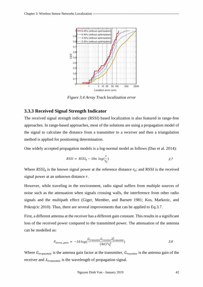
Chapter 3: Wireless Sensor Networks Localization ---------------------------------------------------------------------------------
Nguyen Dinh Van - January 2019 42
Figure 3.4 Array Track localization error
3.3.3 Received Signal Strength Indicator
The received signal strength indicator (RSSI) based localization is also featured in range-free
approaches. In range-based approaches, most of the solutions are using a propagation model of
the signal to calculate the distance from a transmitter to a receiver and then a triangulation
method is applied for positioning determination.
One widely accepted propagation models is a log-normal model as follows (Dao et al. 2014):
𝑅𝑆𝑆𝐼 = 𝑅𝑆𝑆𝐼0 − 10𝑛 𝑙𝑜𝑔(𝑟
𝑟0) 3.7
Where 𝑅𝑆𝑆𝐼0 is the known signal power at the reference distance 𝑟0; and RSSI is the received
signal power at an unknown distance 𝑟.
However, while traveling in the environment, radio signal suffers from multiple sources of
noise such as the attenuation when signals crossing walls, the interference from other radio
signals and the multipath effect (Giger, Member, and Barnett 1981; Kos, Markezic, and
Pokrajcic 2010). Thus, there are several improvements that can be applied to Eq.3.7.
First, a different antenna at the receiver has a different gain constant. This results in a significant
loss of the received power compared to the transmitted power. The attenuation of the antenna
can be modelled as:
𝑃𝑎𝑡𝑒𝑛𝑎_𝑔𝑎𝑖𝑛 = −10 𝑙𝑜𝑔(𝐺𝑡𝑟𝑎𝑛𝑠𝑚𝑖𝑡𝐺𝑟𝑒𝑐𝑒𝑖𝑣𝑒𝜆𝑡𝑟𝑎𝑛𝑠𝑚𝑖𝑡
2
(4𝜋)2𝑟02 ) 3.8
Where 𝐺𝑡𝑟𝑎𝑛𝑠𝑚𝑖𝑡 is the antenna gain factor at the transmitter, 𝐺𝑟𝑒𝑐𝑒𝑖𝑣𝑒 is the antenna gain of the
receiver and 𝜆𝑡𝑟𝑎𝑛𝑠𝑚𝑖𝑡 is the wavelength of propagation signal.

Chapter 3: Wireless Sensor Networks Localization ---------------------------------------------------------------------------------
Nguyen Dinh Van - January 2019 43
Second, during the propagation of signals, there are obstacles such as walls, doors, etc.
Depending on the size, material and position of the obstacles, power loss occurs. Figure 3.5
illustrates one case of obstacles interrupting a signal propagation. In this case, the power loss
can be computed as:
𝑃𝑜𝑏𝑠𝑡𝑎𝑐𝑙𝑒𝑠 = 𝑘𝑑∑𝑑𝑖
𝑐𝑜𝑠 𝛽𝑖
𝑛
𝑖=1
3.9
Where 𝑘𝑑 is the attenuation factor of obstacles’ materials, 𝑑𝑖 is the thickness of obstacles and
𝛽𝑖 is the angle between line-of-sight of transmitter-receiver and the obstacle’s surface.
Figure 3.5 Signal propagation through obstacles (Dao et al. 2014)
Finally, the environment noise is considered as a random variable 𝜒 and the final equation of
signal propagation becomes:
𝑅𝑆𝑆𝐼 = 𝑅𝑆𝑆𝐼0 + 10 𝑙𝑜𝑔(𝐺𝑡𝑟𝑎𝑛𝑠𝑚𝑖𝑡𝐺𝑟𝑒𝑐𝑒𝑖𝑣𝑒𝜆𝑡𝑟𝑎𝑛𝑠𝑚𝑖𝑡
2
(4𝜋)2𝑟02 ) − 10𝑛 𝑙𝑜𝑔 (
𝑟
𝑟0)
− 𝑘𝑑∑𝑑𝑖
𝑐𝑜𝑠 𝛽𝑖
𝑛
𝑖=1
+ 𝜒
3.10
With this method, given a sufficient data of the environment factors (i.e. attenuations of
antennas, obstacles’ materials, a map of the structures and position of each sensors), could be
as accurate as 2.6m (Nguyen et al. 2014; Guan and Ploetz 2017). It is also prone to multiple
sources of noises such as multipath, interference from other radio sources that cannot be
modelled mathematically.
3.4 Range-free approach
3.4.1 Distance Vector Hop
The distance vector hop (DV hop) (Niculescu and Badri Nath 2001) is a three steps localization
process as described below:
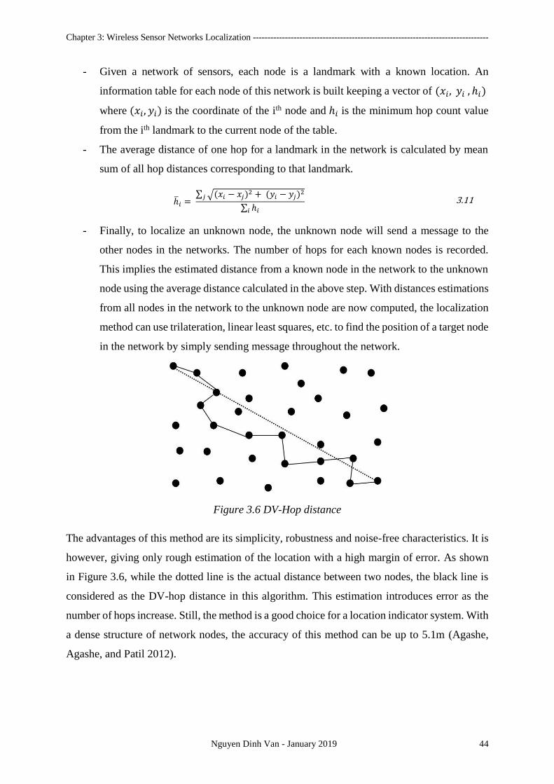
Chapter 3: Wireless Sensor Networks Localization ---------------------------------------------------------------------------------
Nguyen Dinh Van - January 2019 44
- Given a network of sensors, each node is a landmark with a known location. An
information table for each node of this network is built keeping a vector of (𝑥𝑖, 𝑦𝑖 , ℎ𝑖)
where (𝑥𝑖, 𝑦𝑖) is the coordinate of the ith node and ℎ𝑖 is the minimum hop count value
from the ith landmark to the current node of the table.
- The average distance of one hop for a landmark in the network is calculated by mean
sum of all hop distances corresponding to that landmark.
ℎ𝑖 = ∑ √(𝑥𝑖 − 𝑥𝑗)
2 + (𝑦𝑖 − 𝑦𝑗)2
𝑗
∑ ℎ𝑖𝑖
3.11
- Finally, to localize an unknown node, the unknown node will send a message to the
other nodes in the networks. The number of hops for each known nodes is recorded.
This implies the estimated distance from a known node in the network to the unknown
node using the average distance calculated in the above step. With distances estimations
from all nodes in the network to the unknown node are now computed, the localization
method can use trilateration, linear least squares, etc. to find the position of a target node
in the network by simply sending message throughout the network.
Figure 3.6 DV-Hop distance
The advantages of this method are its simplicity, robustness and noise-free characteristics. It is
however, giving only rough estimation of the location with a high margin of error. As shown
in Figure 3.6, while the dotted line is the actual distance between two nodes, the black line is
considered as the DV-hop distance in this algorithm. This estimation introduces error as the
number of hops increase. Still, the method is a good choice for a location indicator system. With
a dense structure of network nodes, the accuracy of this method can be up to 5.1m (Agashe,
Agashe, and Patil 2012).
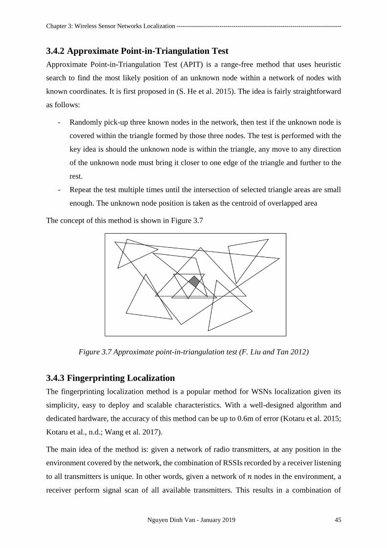
Chapter 3: Wireless Sensor Networks Localization ---------------------------------------------------------------------------------
Nguyen Dinh Van - January 2019 45
3.4.2 Approximate Point-in-Triangulation Test
Approximate Point-in-Triangulation Test (APIT) is a range-free method that uses heuristic
search to find the most likely position of an unknown node within a network of nodes with
known coordinates. It is first proposed in (S. He et al. 2015). The idea is fairly straightforward
as follows:
- Randomly pick-up three known nodes in the network, then test if the unknown node is
covered within the triangle formed by those three nodes. The test is performed with the
key idea is should the unknown node is within the triangle, any move to any direction
of the unknown node must bring it closer to one edge of the triangle and further to the
rest.
- Repeat the test multiple times until the intersection of selected triangle areas are small
enough. The unknown node position is taken as the centroid of overlapped area
The concept of this method is shown in Figure 3.7
Figure 3.7 Approximate point-in-triangulation test (F. Liu and Tan 2012)
3.4.3 Fingerprinting Localization
The fingerprinting localization method is a popular method for WSNs localization given its
simplicity, easy to deploy and scalable characteristics. With a well-designed algorithm and
dedicated hardware, the accuracy of this method can be up to 0.6m of error (Kotaru et al. 2015;
Kotaru et al., n.d.; Wang et al. 2017).
The main idea of the method is: given a network of radio transmitters, at any position in the
environment covered by the network, the combination of RSSIs recorded by a receiver listening
to all transmitters is unique. In other words, given a network of 𝑛 nodes in the environment, a
receiver perform signal scan of all available transmitters. This results in a combination of

Chapter 3: Wireless Sensor Networks Localization ---------------------------------------------------------------------------------
Nguyen Dinh Van - January 2019 46
signals strengths and transmitters ID (most commonly transmitter’s MAC address) which is
unique for any location in the environment. In Figure 3.8, the receiver is scanning for RSSI
from a total of 5 transmitters in the environment, each with a different MAC address.
Consequently, the unique feature vector of this location 𝑥, 𝑦 will be written as:
(𝑀𝐴𝐶1, 𝑅𝑆𝑆𝐼1), (𝑀𝐴𝐶2, 𝑅𝑆𝑆𝐼2), . . , (𝑀𝐴𝐶5, 𝑅𝑆𝑆𝐼5) → 𝑥, 𝑦 3.12
By building a database of multiple locations’ feature vectors in the environment, a localization
process later can simply be carried out with a classification algorithm of real-time RSSIs scan.
Each location with feature vectors registered in the database will be called a fingerprint.
TransmitterMAC address 1
TransmitterMAC address 2
TransmitterMAC address 3
TransmitterMAC address 4
TransmitterMAC address 5
Receiver
Figure 3.8 Fingerprinting localization concept
There are several advantages of this method. Database building of feature vectors is a relatively
simple process. It does not require the receiver to actually connect to the transmitter and
exchange messages. There is also no need of transmitters’ positions information to be known.
One can simply perform standard scanning action from the receiver and store the information
received. Any commercial off-the-shelf device should be able to perform such task which
makes deploying this solution feasible and scalable.
On the other hand, this method suffers from noise and changes in the environment setup. Any
major change of the environment is likely to decrease localization accuracy. At the same time,
depending on radio frequency of the transmitters and receivers, the initial assumption of unique
feature for a unique position is likely to vary. Ultra-wideband radio frequency devices tend to
perform much better than other signals such as Wi-Fi, cellular (Alarifi et al. 2016; “Infsoft
Ultra-Wideband Technology for Indoor Positioning” 2018). However, unlike other classical
radio devices, the ultra-wideband devices are not commonly available in the environment and
has much shorter range of coverage.
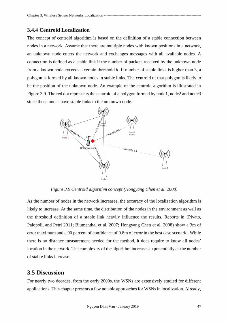
Chapter 3: Wireless Sensor Networks Localization ---------------------------------------------------------------------------------
Nguyen Dinh Van - January 2019 47
3.4.4 Centroid Localization
The concept of centroid algorithm is based on the definition of a stable connection between
nodes in a network. Assume that there are multiple nodes with known positions in a network,
an unknown node enters the network and exchanges messages with all available nodes. A
connection is defined as a stable link if the number of packets received by the unknown node
from a known node exceeds a certain threshold ℎ. If number of stable links is higher than 3, a
polygon is formed by all known nodes in stable links. The centroid of that polygon is likely to
be the position of the unknown node. An example of the centroid algorithm is illustrated in
Figure 3.9. The red dot represents the centroid of a polygon formed by node1, node2 and node3
since those nodes have stable links to the unknown node.
Node 1
Node 1
Node 1
Node 1
Node 1
Unknown node
Figure 3.9 Centroid algorithm concept (Hongyang Chen et al. 2008)
As the number of nodes in the network increases, the accuracy of the localization algorithm is
likely to increase. At the same time, the distribution of the nodes in the environment as well as
the threshold definition of a stable link heavily influence the results. Reports in (Pivato,
Palopoli, and Petri 2011; Blumenthal et al. 2007; Hongyang Chen et al. 2008) show a 3m of
error maximum and a 90 percent of confidence of 0.8m of error in the best case scenario. While
there is no distance measurement needed for the method, it does require to know all nodes’
location in the network. The complexity of the algorithm increases exponentially as the number
of stable links increase.
3.5 Discussion
For nearly two decades, from the early 2000s, the WSNs are extensively studied for different
applications. This chapter presents a few notable approaches for WSNs in localization. Already,
Chapter 3: Wireless Sensor Networks Localization ---------------------------------------------------------------------------------
Nguyen Dinh Van - January 2019 48
it is clear that the potential of WSNs in localization is high. With a wide range of coverage, the
availability of sensors and their increasing accuracy, WSNs become a preferred solution for
both GPS-denied and GPS-aided environment.
However, in context of intelligent vehicles localization, there are very few studies in recent
years. A study in (Moussawi 2012) presents a cooperative localization strategy of vehicles using
WSNs. Using methods such as TOA, RSSI with Ultra-Wideband technology, the study achieves
a RMSE localization accuracy of 2m. Another cooperative strategy is mentioned in (Garip et
al. 2017) where vehicles are nodes within a WSNs. This system is able to identify a vehicle
within 10m range. A WLAN-based localization system for the parking area is introduced in
(Mauro et al. 2009) where a fingerprinting localization method is used. The accuracy of the
method is around 7.3m. A university campus localization method of vehicles using wireless
network is implemented in (Hernandez et al. 2017) results in 9.34m of localization accuracy.
As mentioned in Section 2.6, the balance between complexity and accuracy is essential for a
true autonomy. Thus a two levels localization system is proposed. Studies in this chapter
suggest that a WSN localization solution is suitable for a global localization layer for the
following reasons:
- WSN solutions tend to have a wide coverage range due to radio signals characteristics.
Depending on the sensors, it may or may not require Line-of-Sights (LoS). Unlike other
sensors such as ultrasonic, cameras, lasers where LoS is extremely important. This
makes WSNs a suitable candidate for obstructed areas global localization.
- WSN solutions often do not require much investment but still offer a relatively high
accuracy of localization. The availability, performance of wireless sensors is increasing
and so to theirs qualities. However, the accuracy of those solutions is still in order of a
meter. Hence, it is not yet fit for local localization level.
- Due to signals transmission and messages exchange happening in a complex network,
the localization rate for a WSN solution is more often low (around 1Hz). This is one of
the main reasons why WSNs are not yet applied for intelligent vehicle navigation at
high speed. Still, at a relatively low speed of navigation, it is feasible for a WSNs to
keep track of an intelligent vehicle.
Given the arguments listed above, this thesis will propose and develop a WSN solution for a
low-speed vehicle localization in GPS-denied area. This solution will be a global level
localization system. Furthermore, with a fusion strategy with other sensors information such as

Chapter 3: Wireless Sensor Networks Localization ---------------------------------------------------------------------------------
Nguyen Dinh Van - January 2019 49
IMU or laser-based SLAM, the system is expected to achieve a significant localization
accuracy.
50
4. WI-FI FINGERPRINTING LOCALIZATION
Résumé
En comparant différentes approches de localisation des WSN, une méthode de prise d'empreinte
est choisie car elle satisfait aux quatre critères énoncés dans la section 1.2, à savoir la
disponibilité, l'évolutivité, l'universalité et la précision.
Le concept général de la localisation d'empreintes digitales Wi-Fi est présenté à la section 3.4.3.
Il existe deux phases pour cette méthode: une phase hors ligne et une phase en ligne.
Dans la phase hors ligne, une base de données d'empreintes digitales (FP) est construite.
Comme défini dans la section 3.4.3, une empreinte digitale peut être n'importe quel
emplacement de l'environnement ciblé avec des coordonnées connues. Chaque enregistrement
dans la base de données d'empreintes digitales est un mappage des coordonnées d'une empreinte
digitale et de tous les RSSI numérisés à cette position. Dans la Figure 4.1, chaque point bleu
est une empreinte digitale (FP) avec des coordonnées connues. À un certain FP, les RSSI des
cinq points d'accès (AP0, AP1, .., AP4) sont enregistrés et mis en correspondance avec ses
coordonnées. Répétez cette procédure pour tous les PF de l'environnement pour établir la base
de données d'empreintes digitales. Un enregistrement dans cette base de données est écrit
comme dans Eq.4.1.
Dans la phase en ligne où l’estimation de la localisation est effectuée, le véhicule se déplacera
dans l’environnement tout en recherchant les RSSI des points d’accès environnants. Une
fonction de vraisemblance basée sur les données de la phase hors ligne est définie par Eq.4.3.
En général, l'empreinte digitale avec le score de vraisemblance le plus élevé sera choisie comme
emplacement estimé.
Chapter 4: Wi-Fi fingerprinting localization ------------------------------------------------------------------------------------------
Nguyen Dinh Van - January 2019 51
Récemment, plusieurs tentatives d'utilisation du concept d'empreinte digitale Wi-Fi ont été
utilisées pour déterminer la position d'un véhicule. Certaines approches utilisent les
smartphones des utilisateurs pour aider et guider le conducteur vers un parking. D'autres
approches visent directement des véhicules intelligents avec des capteurs montés sur des
véhicules. Selon le choix des capteurs (smartphone ou capteurs montés), la précision du système
de localisation risque d'être affectée. Le chapitre présente quatre études notables. Ces études
permettent d’atteindre environ 3-4 m d’erreur de localisation moyenne.
Après avoir examiné ces études, nous avons identifié deux problèmes majeurs concernant la
méthode de localisation d'empreintes digitales Wi-Fi pour les véhicules: une fréquence
d'échantillonnage faible du balayage Wi-Fi et une forte variance des forces du signal reçu. Pour
résoudre ces problèmes, des modifications sont proposées aux phases hors ligne et en ligne.
Dans la phase hors ligne, une base de données d'apprentissage hybride est mise en œuvre pour
résoudre le problème de la vitesse de déplacement. De plus, un réseau de neurones d'ensemble
(Dietterich 2000) pour la fonction de vraisemblance de phase en ligne est déployé pour résoudre
le problème des signaux à forte variance.
La base de données hybride hors ligne est proposée avec une nouvelle définition d'empreinte
digitale et un mélange d'analyses dynamiques et statiques. La distance entre deux lieux
d'initiation et de fin de l'analyse est appelée une plage d'analyse. En fonction de la vitesse de
déplacement de la cible, la plage de balayage peut également varier. Ainsi, une nouvelle
définition d'empreinte digitale en tant que cercle est modélisée dans Eq.4.4. De plus, pour
modéliser correctement les signaux reçus de la phase en ligne, en plus de la collecte classique
de données statiques, des signaux sont également enregistrés pendant le déplacement des
véhicules dans l'emplacement de l'empreinte digitale.
Dans la phase en ligne, une fonction de vraisemblance h est requise pour évaluer le vecteur
RSSI d'entrée en temps réel. L'idée d'utiliser plusieurs modèles d'apprentissage pour améliorer
les performances d'un seul est proposée dans (Krogh, Anders Jesper, 1995; Breiman, 1996;
Hansen et Salamon, 1990). Dans certaines conditions, la combinaison d'estimateurs divers, non
corrélés mais précis, devrait donner de meilleures performances qu'un seul. Cette section
présente la stratégie d'ensemble visant à améliorer les résultats prévus (Eq.4.9 à Eq.4.13).
Les expériences relatives à la méthode proposée sont effectuées dans une place de parking
ouverte du campus de l’INRIA Rocquencourt. En raison de la difficulté d’avoir un parking
couvert pour les expériences, l’espace extérieur est utilisé. En même temps, ce parking extérieur

Chapter 4: Wi-Fi fingerprinting localization ------------------------------------------------------------------------------------------
Nguyen Dinh Van - January 2019 52
bénéficie d’un RTK-GPS précis pour la vérité du terrain. Cela permet une meilleure évaluation
du système. La zone d’essai est illustrée à la figure 4.16. Il existe deux véhicules dans les
expériences: un Cybercar bleu conçu comme un prototype pour les véhicules intelligents et une
Citroën C1 rouge modifiée à des fins expérimentales.
Tout d'abord, une étude de la zone de test est réalisée pour comprendre les caractéristiques de
la méthode. Les résultats de cette enquête suggèrent qu'il existe une forte corrélation entre la
force moyenne du signal Wi-Fi et la précision du résultat de la localisation. Ainsi, avec une
attente réaliste d’une bonne force de signal moyenne dans le scénario réel, la zone d’essai est
alors définie. Dans la figure 4.23, les empreintes digitales sont marquées d'un cercle rouge. La
distance moyenne entre deux empreintes digitales adjacentes est de 6,1 m, ce qui correspond à
la limite supérieure de l'inter-distance entre les empreintes digitales décrite à la section 4.1.
Avec cette distance, il ne faut que 25 empreintes digitales pour couvrir la zone de test. Pour
chaque empreinte digitale, 60 analyses statiques et 20 analyses dynamiques sont enregistrées
pour la base de données hors connexion. Un total de 156 points d'accès avec différentes adresses
MAC est détecté sur 25 empreintes digitales. nous définissons ensuite un bon résultat de
classification du réseau de neurones comme étant les empreintes digitales les plus proches de
la vérité au sol en distance euclidienne. Comme mentionné dans l'équation 4.18, le résultat de
Ensemble Neural Network est une liste des indices d’empreintes digitales et de leur confiance.
Supposons que l'empreinte digitale de confiance la plus élevée est choisie comme résultat final
de la classification. Un bon résultat de la classification doit satisfaire à l'Eq. 4.22. Pendant un
an, avec plus de 60 expériences menées, la méthode proposée a surperformé toutes les solutions
existantes et a une précision moyenne de 2,25 m.
4.1 Introduction
As discussed in Chapter 2, there is a need for a global positioning system of intelligent vehicles
in the GPS-denied area. Given the characteristics of the WSN, Section 3.5 pointed out that it is
a feasible solution for the quest. However, choosing an approach for such a system needs to be
considered carefully. In the scope of the thesis, four criteria have been identified: availability,
scalability, universality and accuracy. A quick comparison of WSNs localization approaches
highlighted in Chapter 3 is shown in Table 4. Note that this comparison takes into account only
approaches without any hardware modification.
Although such comparison may change depending on sensors type as well as the targeted
environment, it gives an overview of these approaches under the four selected criteria. In the
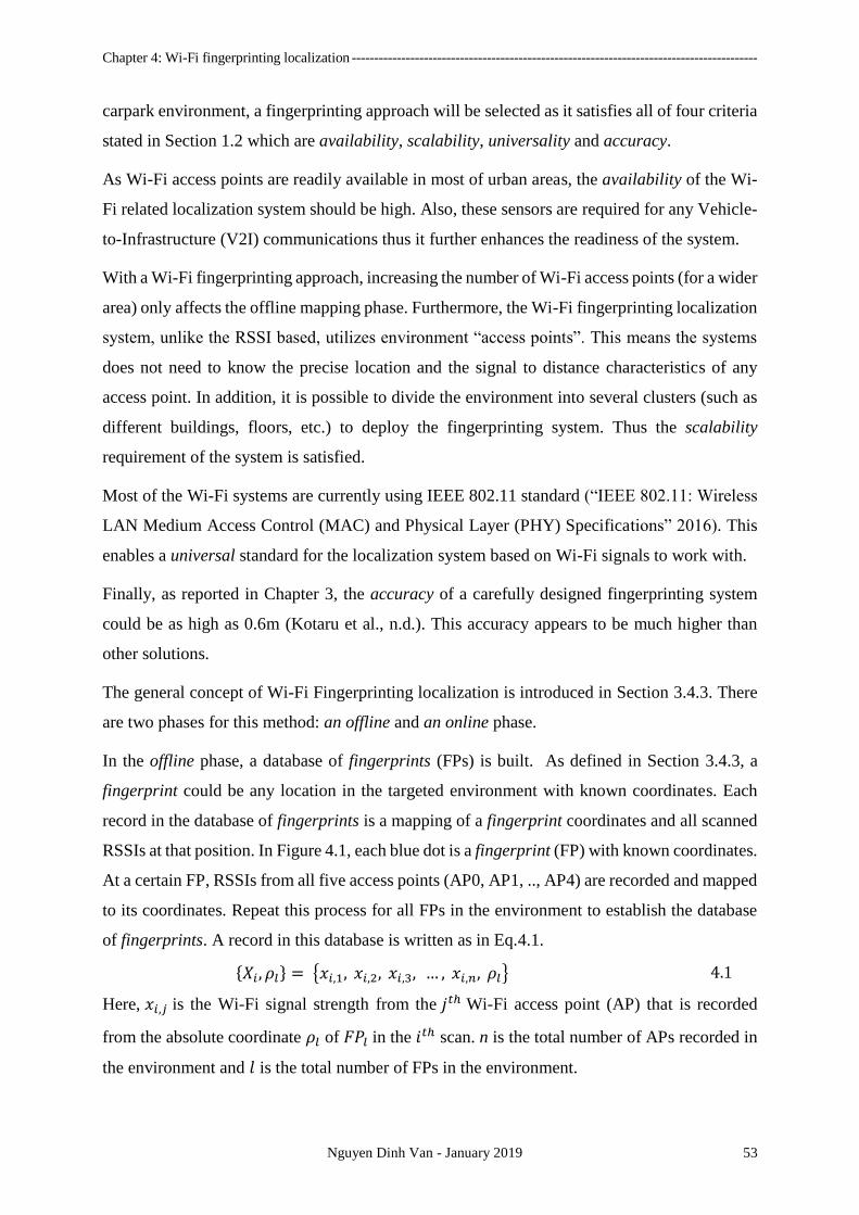
Chapter 4: Wi-Fi fingerprinting localization ------------------------------------------------------------------------------------------
Nguyen Dinh Van - January 2019 53
carpark environment, a fingerprinting approach will be selected as it satisfies all of four criteria
stated in Section 1.2 which are availability, scalability, universality and accuracy.
As Wi-Fi access points are readily available in most of urban areas, the availability of the Wi-
Fi related localization system should be high. Also, these sensors are required for any Vehicle-
to-Infrastructure (V2I) communications thus it further enhances the readiness of the system.
With a Wi-Fi fingerprinting approach, increasing the number of Wi-Fi access points (for a wider
area) only affects the offline mapping phase. Furthermore, the Wi-Fi fingerprinting localization
system, unlike the RSSI based, utilizes environment “access points”. This means the systems
does not need to know the precise location and the signal to distance characteristics of any
access point. In addition, it is possible to divide the environment into several clusters (such as
different buildings, floors, etc.) to deploy the fingerprinting system. Thus the scalability
requirement of the system is satisfied.
Most of the Wi-Fi systems are currently using IEEE 802.11 standard (“IEEE 802.11: Wireless
LAN Medium Access Control (MAC) and Physical Layer (PHY) Specifications” 2016). This
enables a universal standard for the localization system based on Wi-Fi signals to work with.
Finally, as reported in Chapter 3, the accuracy of a carefully designed fingerprinting system
could be as high as 0.6m (Kotaru et al., n.d.). This accuracy appears to be much higher than
other solutions.
The general concept of Wi-Fi Fingerprinting localization is introduced in Section 3.4.3. There
are two phases for this method: an offline and an online phase.
In the offline phase, a database of fingerprints (FPs) is built. As defined in Section 3.4.3, a
fingerprint could be any location in the targeted environment with known coordinates. Each
record in the database of fingerprints is a mapping of a fingerprint coordinates and all scanned
RSSIs at that position. In Figure 4.1, each blue dot is a fingerprint (FP) with known coordinates.
At a certain FP, RSSIs from all five access points (AP0, AP1, .., AP4) are recorded and mapped
to its coordinates. Repeat this process for all FPs in the environment to establish the database
of fingerprints. A record in this database is written as in Eq.4.1.
𝑋𝑖, 𝜌𝑙 = 𝑥𝑖,1, 𝑥𝑖,2, 𝑥𝑖,3, … , 𝑥𝑖,𝑛, 𝜌𝑙 4.1
Here, 𝑥𝑖,𝑗 is the Wi-Fi signal strength from the 𝑗𝑡ℎ Wi-Fi access point (AP) that is recorded
from the absolute coordinate 𝜌𝑙 of 𝐹𝑃𝑙 in the 𝑖𝑡ℎ scan. n is the total number of APs recorded in
the environment and 𝑙 is the total number of FPs in the environment.
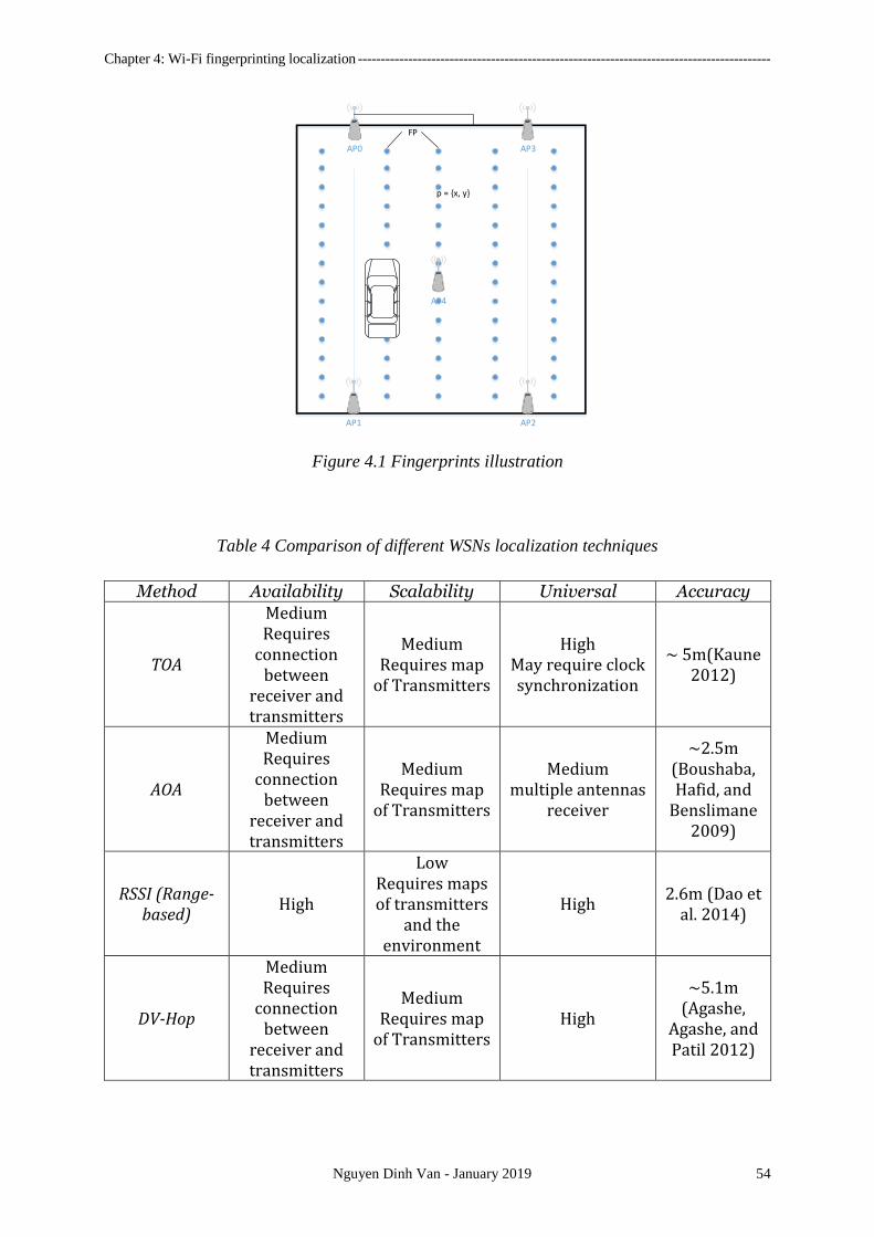
Chapter 4: Wi-Fi fingerprinting localization ------------------------------------------------------------------------------------------
Nguyen Dinh Van - January 2019 54
AP0 AP3
AP1 AP2
AP4
FP
p = x, y
Figure 4.1 Fingerprints illustration
Table 4 Comparison of different WSNs localization techniques
Method Availability Scalability Universal Accuracy
TOA
Medium Requires
connection between
receiver and transmitters
Medium Requires map
of Transmitters
High May require clock synchronization
~ 5m(Kaune 2012)
AOA
Medium Requires
connection between
receiver and transmitters
Medium Requires map
of Transmitters
Medium multiple antennas
receiver
~2.5m (Boushaba, Hafid, and
Benslimane 2009)
RSSI (Range-based)
High
Low Requires maps of transmitters
and the environment
High 2.6m (Dao et
al. 2014)
DV-Hop
Medium Requires
connection between
receiver and transmitters
Medium Requires map
of Transmitters High
~5.1m (Agashe,
Agashe, and Patil 2012)
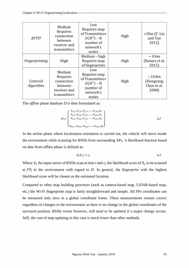
Chapter 4: Wi-Fi fingerprinting localization ------------------------------------------------------------------------------------------
Nguyen Dinh Van - January 2019 55
APTIT
Medium Requires
connection between
receiver and transmitters
Low Requires map
of Transmitters 𝑂(𝑁2) – N number of network’s
nodes
High
>20m (F. Liu and Tan 2012)
Fingerprinting High Medium – high Requires map of fingerprints
High ~ 0.6m
(Kotaru et al. 2015)
Centroid Algorithm
Medium Requires
connection between
receiver and transmitters
Low Requires map
of Transmitters 𝑂(𝑁2) – N number of network’s
nodes
High
~10.8m (Hongyang Chen et al.
2008)
The offline phase database D is then formulated as:
D =
𝑥1,1, 𝑥1,2, 𝑥1,3, … , 𝑥1,𝑛, 𝜌1𝑥2,1, 𝑥2,2, 𝑥2,3, … , 𝑥2,𝑛 , 𝜌1𝑥3,1, 𝑥3,2, 𝑥3,3, … , 𝑥3,𝑛 , 𝜌2
⋮𝑥𝑚,1, 𝑥𝑚,2, 𝑥𝑚,3, … , 𝑥𝑚,𝑛, 𝜌𝑙
4.2
In the online phase where localization estimation is carried out, the vehicle will move inside
the environment while scanning for RSSIs from surrounding APs. A likelihood function based
on data from offline phase is defined as:
ℎ(𝑋𝑡) = 𝑐𝑙 4.3
Where Xt the input vector of RSSIs scan at time t and 𝑐𝑙 the likelihood score of Xt to be scanned
at 𝐹𝑃𝑙 in the environment with regard to D. In general, the fingerprint with the highest
likelihood score will be chosen as the estimated location.
Compared to other map building processes (such as camera-based map, LiDAR-based map,
etc.) the Wi-Fi fingerprints map is fairly straightforward and simple. All FPs coordinates can
be measured only once in a global coordinate frame. These measurements remain correct
regardless of changes in the environment as there is no change in the global coordinates of the
surveyed position. RSSIs vector however, will need to be updated if a major change occurs.
Still, the cost of map updating in this case is much lower than other methods.
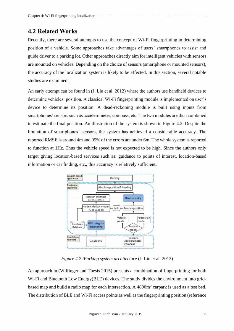
Chapter 4: Wi-Fi fingerprinting localization ------------------------------------------------------------------------------------------
Nguyen Dinh Van - January 2019 56
4.2 Related Works
Recently, there are several attempts to use the concept of Wi-Fi fingerprinting in determining
position of a vehicle. Some approaches take advantages of users’ smartphones to assist and
guide driver to a parking lot. Other approaches directly aim for intelligent vehicles with sensors
are mounted on vehicles. Depending on the choice of sensors (smartphone or mounted sensors),
the accuracy of the localization system is likely to be affected. In this section, several notable
studies are examined.
An early attempt can be found in (J. Liu et al. 2012) where the authors use handheld devices to
determine vehicles’ position. A classical Wi-Fi fingerprinting module is implemented on user’s
device to determine its position. A dead-reckoning module is built using inputs from
smartphones’ sensors such as accelerometer, compass, etc. The two modules are then combined
to estimate the final position. An illustration of the system is shown in Figure 4.2. Despite the
limitation of smartphones’ sensors, the system has achieved a considerable accuracy. The
reported RMSE is around 4m and 95% of the errors are under 6m. The whole system is reported
to function at 1Hz. Thus the vehicle speed is not expected to be high. Since the authors only
target giving location-based services such as: guidance to points of interest, location-based
information or car finding, etc., this accuracy is relatively sufficient.
Figure 4.2 iParking system architecture (J. Liu et al. 2012)
An approach in (Wilfinger and Thesis 2015) presents a combination of fingerprinting for both
Wi-Fi and Bluetooth Low Energy(BLE) devices. The study divides the environment into grid-
based map and build a radio map for each intersection. A 4800m2 carpark is used as a test bed.
The distribution of BLE and Wi-Fi access points as well as the fingerprinting position (reference

Chapter 4: Wi-Fi fingerprinting localization ------------------------------------------------------------------------------------------
Nguyen Dinh Van - January 2019 57
points) are shown in Figure 4.3. A total of 60 BLE access points and 10 Wi-Fi access points are
used. The BLE sensors are operated at 10Hz while the Wi-Fi scan is performed at a rate of 1Hz.
Three databases of fingerprint for Wi-Fi, BLE and a combination both Wi-Fi and BLE are built
to evaluate the accuracy of each method. The final result for localization is shown in Table 5.
The vehicle speed in this research is around 10km/h (or 2.8m/s). The fingerprinting algorithm
in this work is referred as a simple standard fingerprinting localization algorithm.
Figure 4.3 Thondorf carpark (Wilfinger and Thesis 2015)
The position error for a test run is shown in Figure 4.4. In this figure, the WLAN fingerprinting
localization appears to be highly inaccurate. The BLE shows a much better result as the
functioning rate and number of BLE units in the environment is significantly higher than those
in WLAN. The combination result of both solutions shows a slightly improvement compared
to the BLE method.
Figure 4.4 Time series for a test run (Wilfinger and Thesis 2015)
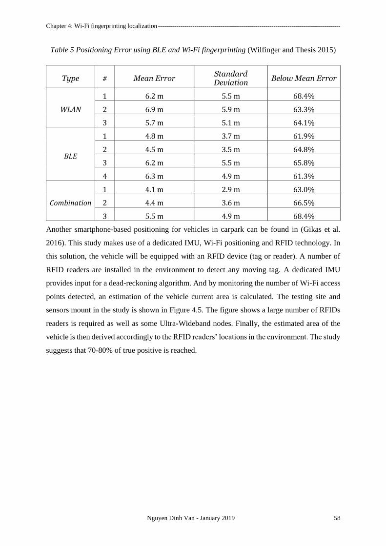
Chapter 4: Wi-Fi fingerprinting localization ------------------------------------------------------------------------------------------
Nguyen Dinh Van - January 2019 58
Table 5 Positioning Error using BLE and Wi-Fi fingerprinting (Wilfinger and Thesis 2015)
Type # Mean Error Standard Deviation
Below Mean Error
WLAN
1 6.2 m 5.5 m 68.4%
2 6.9 m 5.9 m 63.3%
3 5.7 m 5.1 m 64.1%
BLE
1 4.8 m 3.7 m 61.9%
2 4.5 m 3.5 m 64.8%
3 6.2 m 5.5 m 65.8%
4 6.3 m 4.9 m 61.3%
Combination
1 4.1 m 2.9 m 63.0%
2 4.4 m 3.6 m 66.5%
3 5.5 m 4.9 m 68.4%
Another smartphone-based positioning for vehicles in carpark can be found in (Gikas et al.
2016). This study makes use of a dedicated IMU, Wi-Fi positioning and RFID technology. In
this solution, the vehicle will be equipped with an RFID device (tag or reader). A number of
RFID readers are installed in the environment to detect any moving tag. A dedicated IMU
provides input for a dead-reckoning algorithm. And by monitoring the number of Wi-Fi access
points detected, an estimation of the vehicle current area is calculated. The testing site and
sensors mount in the study is shown in Figure 4.5. The figure shows a large number of RFIDs
readers is required as well as some Ultra-Wideband nodes. Finally, the estimated area of the
vehicle is then derived accordingly to the RFID readers’ locations in the environment. The study
suggests that 70-80% of true positive is reached.
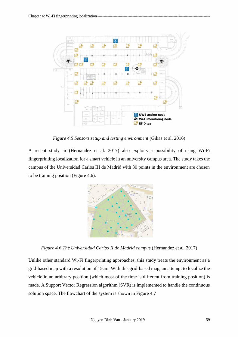
Chapter 4: Wi-Fi fingerprinting localization ------------------------------------------------------------------------------------------
Nguyen Dinh Van - January 2019 59
Figure 4.5 Sensors setup and testing environment (Gikas et al. 2016)
A recent study in (Hernandez et al. 2017) also exploits a possibility of using Wi-Fi
fingerprinting localization for a smart vehicle in an university campus area. The study takes the
campus of the Universidad Carlos III de Madrid with 30 points in the environment are chosen
to be training position (Figure 4.6).
Figure 4.6 The Universidad Carlos II de Madrid campus (Hernandez et al. 2017)
Unlike other standard Wi-Fi fingerprinting approaches, this study treats the environment as a
grid-based map with a resolution of 15cm. With this grid-based map, an attempt to localize the
vehicle in an arbitrary position (which most of the time is different from training position) is
made. A Support Vector Regression algorithm (SVR) is implemented to handle the continuous
solution space. The flowchart of the system is shown in Figure 4.7

Chapter 4: Wi-Fi fingerprinting localization ------------------------------------------------------------------------------------------
Nguyen Dinh Van - January 2019 60
Figure 4.7 General architecture of the system (Hernandez et al. 2017)
The experiments are carried out with 175 Wi-Fi access points recorded, an intelligent vehicle
operated at 4.86km/h speed moving through a path of 145m. Final results show an average
localization error at best case is 6.18m.
Figure 4.8 Cumulative Distribution of Error (Hernandez et al. 2017)
The latest research on the Wi-Fi fingerprinting for intelligent vehicle is presented in (Ang
2018). This research is particular interesting for their ambitious goal of replacing the GPS signal
in urban area with the existing Wi-Fi infrastructure. Due to the obstruction in urban area, the
GPS signal is expected to be poor. Thus, a Wi-Fi fingerprinting localization system is deployed
in the crowded streets of Singapore in this research to improve the absolute localization. The
research, however, uses a Nexus 5 android device to capture Wi-Fi signal instead of mounting
sensors on the vehicle. The test run and area of experiment is shown in Figure 4.9. An early
result is obtained with 80% of errors are under 15m.The cumulative distribution of error is
shown in Figure 4.10. Although such result is still large, it shows promising sign of using the
method in a complex environment such as urban area. Given that the authors use a phone instead
of a dedicated Wi-Fi receiver for the experiments, there is still room for improvement.
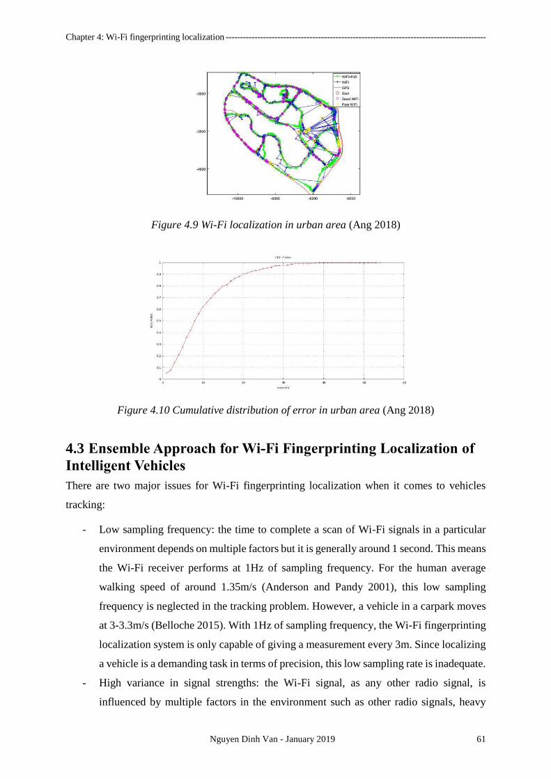
Chapter 4: Wi-Fi fingerprinting localization ------------------------------------------------------------------------------------------
Nguyen Dinh Van - January 2019 61
Figure 4.9 Wi-Fi localization in urban area (Ang 2018)
Figure 4.10 Cumulative distribution of error in urban area (Ang 2018)
4.3 Ensemble Approach for Wi-Fi Fingerprinting Localization of
Intelligent Vehicles
There are two major issues for Wi-Fi fingerprinting localization when it comes to vehicles
tracking:
- Low sampling frequency: the time to complete a scan of Wi-Fi signals in a particular
environment depends on multiple factors but it is generally around 1 second. This means
the Wi-Fi receiver performs at 1Hz of sampling frequency. For the human average
walking speed of around 1.35m/s (Anderson and Pandy 2001), this low sampling
frequency is neglected in the tracking problem. However, a vehicle in a carpark moves
at 3-3.3m/s (Belloche 2015). With 1Hz of sampling frequency, the Wi-Fi fingerprinting
localization system is only capable of giving a measurement every 3m. Since localizing
a vehicle is a demanding task in terms of precision, this low sampling rate is inadequate.
- High variance in signal strengths: the Wi-Fi signal, as any other radio signal, is
influenced by multiple factors in the environment such as other radio signals, heavy

Chapter 4: Wi-Fi fingerprinting localization ------------------------------------------------------------------------------------------
Nguyen Dinh Van - January 2019 62
metal obstacles, etc. this results in a high variance of RSSIs which in turn lowers the
precision of the likelihood function. Also, in case of vehicles’ movement, due to the
higher speed of movement, this issue becomes much more significant in comparison to
the pedestrians’ movement.
To address these issues, changes in both offline and online phases are proposed. In the offline
phase, a hybrid learning database is implemented to overcome the movement speed issue.
Furthermore, an ensemble neural network(Dietterich 2000) for the online phase likelihood
function is deployed to solve the high variance signals problem.
4.3.1 Hybrid Database Offline Phase
In the classical approach of Wi-Fi fingerprinting localization, the mapping Xi, ρl in the offline
phase is perceived as a representative feature vector Xi of the fingerprint ρl. The underlying
assumption for this mapping is at a fixed location, its feature vector is unique. However, as this
database is used for evaluating the online phase likelihood function, there is an issue with the
online input data.
Human speed scan range
Scan
Initia
tion
Scan
com
ple
te
Vehicle speed scan range
Fingerprint
Figure 4.11 Online scan range for different speeds
Consider a scenario as in Figure 4.11, the fixed location fingerprint is defined in the offline
phase and illustrated as the circle in the figure. With 1Hz of sampling frequency, a Wi-Fi scan
is initiated at a certain position and terminated at a different one. The distance between two
locations of scan initiation and termination is called a scan range. Depending on the movement
speed of the target, the scan range can also vary. With an average of 1.35m/s for human walking
speed, the scan range for a human walking case is also around 1.35m. Thus, a signal vector Xt
in the online phase is the feature vector of a path but not a fixed position. By reducing this path
to a fingerprint location in the likelihood function, an error of localization is introduced. When
it comes to the targeted scenario in this thesis, a vehicle in a carpark has 3.3m/s average speed
which results in an approximately 3.3m of scan range. This is a significant distance for the
vehicle navigation task. Hence, a new hybrid database of offline phase database is proposed.
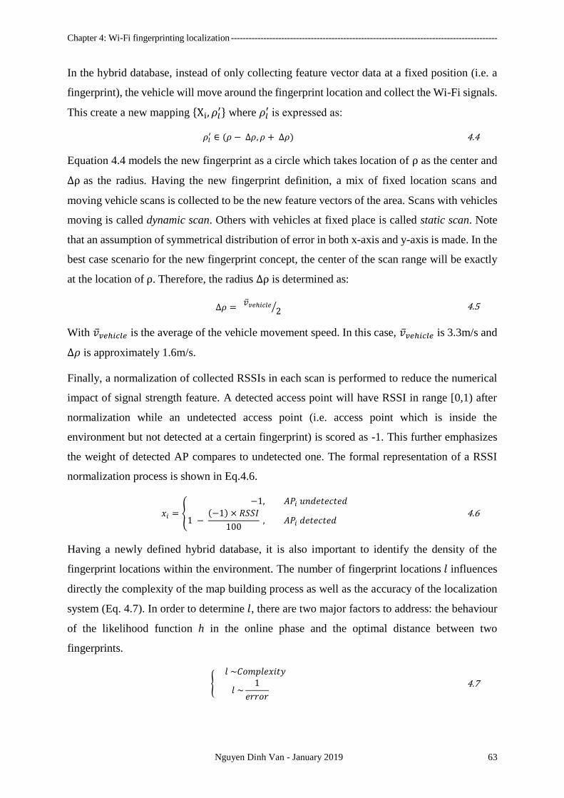
Chapter 4: Wi-Fi fingerprinting localization ------------------------------------------------------------------------------------------
Nguyen Dinh Van - January 2019 63
In the hybrid database, instead of only collecting feature vector data at a fixed position (i.e. a
fingerprint), the vehicle will move around the fingerprint location and collect the Wi-Fi signals.
This create a new mapping Xi, 𝜌𝑙′ where 𝜌𝑙
′ is expressed as:
𝜌𝑙′ ∈ (𝜌 − ∆𝜌, 𝜌 + ∆𝜌) 4.4
Equation 4.4 models the new fingerprint as a circle which takes location of ρ as the center and
∆ρ as the radius. Having the new fingerprint definition, a mix of fixed location scans and
moving vehicle scans is collected to be the new feature vectors of the area. Scans with vehicles
moving is called dynamic scan. Others with vehicles at fixed place is called static scan. Note
that an assumption of symmetrical distribution of error in both x-axis and y-axis is made. In the
best case scenario for the new fingerprint concept, the center of the scan range will be exactly
at the location of ρ. Therefore, the radius ∆ρ is determined as:
∆𝜌 = 𝑣𝑒ℎ𝑖𝑐𝑙𝑒
2⁄ 4.5
With 𝑣𝑒ℎ𝑖𝑐𝑙𝑒 is the average of the vehicle movement speed. In this case, 𝑣𝑒ℎ𝑖𝑐𝑙𝑒 is 3.3m/s and
∆𝜌 is approximately 1.6m/s.
Finally, a normalization of collected RSSIs in each scan is performed to reduce the numerical
impact of signal strength feature. A detected access point will have RSSI in range [0,1) after
normalization while an undetected access point (i.e. access point which is inside the
environment but not detected at a certain fingerprint) is scored as -1. This further emphasizes
the weight of detected AP compares to undetected one. The formal representation of a RSSI
normalization process is shown in Eq.4.6.
𝑥𝑖 =
−1, 𝐴𝑃𝑖 𝑢𝑛𝑑𝑒𝑡𝑒𝑐𝑡𝑒𝑑
1 − (−1) × 𝑅𝑆𝑆𝐼
100 , 𝐴𝑃𝑖 𝑑𝑒𝑡𝑒𝑐𝑡𝑒𝑑
4.6
Having a newly defined hybrid database, it is also important to identify the density of the
fingerprint locations within the environment. The number of fingerprint locations 𝑙 influences
directly the complexity of the map building process as well as the accuracy of the localization
system (Eq. 4.7). In order to determine 𝑙, there are two major factors to address: the behaviour
of the likelihood function h in the online phase and the optimal distance between two
fingerprints.
𝑙 ~𝐶𝑜𝑚𝑝𝑙𝑒𝑥𝑖𝑡𝑦
𝑙 ~1
𝑒𝑟𝑟𝑜𝑟
4.7
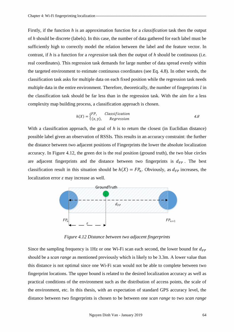
Chapter 4: Wi-Fi fingerprinting localization ------------------------------------------------------------------------------------------
Nguyen Dinh Van - January 2019 64
Firstly, if the function h is an approximation function for a classification task then the output
of h should be discrete (labels). In this case, the number of data gathered for each label must be
sufficiently high to correctly model the relation between the label and the feature vector. In
contrast, if h is a function for a regression task then the output of h should be continuous (i.e.
real coordinates). This regression task demands for large number of data spread evenly within
the targeted environment to estimate continuous coordinates (see Eq. 4.8). In other words, the
classification task asks for multiple data on each fixed position while the regression task needs
multiple data in the entire environment. Therefore, theoretically, the number of fingerprints 𝑙 in
the classification task should be far less than in the regression task. With the aim for a less
complexity map building process, a classification approach is chosen.
ℎ(𝑋) = 𝐹𝑃, 𝐶𝑙𝑎𝑠𝑠𝑖𝑓𝑖𝑐𝑎𝑡𝑖𝑜𝑛
(𝑥, 𝑦), 𝑅𝑒𝑔𝑟𝑒𝑠𝑠𝑖𝑜𝑛 4.8
With a classification approach, the goal of h is to return the closest (in Euclidian distance)
possible label given an observation of RSSIs. This results in an accuracy constraint: the further
the distance between two adjacent positions of Fingerprints the lower the absolute localization
accuracy. In Figure 4.12, the green dot is the real position (ground truth), the two blue circles
are adjacent fingerprints and the distance between two fingerprints is 𝑑𝐹𝑃 . The best
classification result in this situation should be ℎ(𝑋) = 𝐹𝑃𝑛. Obviously, as 𝑑𝐹𝑃 increases, the
localization error 𝜀 may increase as well.
𝐹𝑃𝑛 𝐹𝑃𝑛+1
GroundTruth
𝑑𝐹𝑃
𝜀
Figure 4.12 Distance between two adjacent fingerprints
Since the sampling frequency is 1Hz or one Wi-Fi scan each second, the lower bound for 𝑑𝐹𝑃
should be a scan range as mentioned previously which is likely to be 3.3m. A lower value than
this distance is not optimal since one Wi-Fi scan would not be able to complete between two
fingerprint locations. The upper bound is related to the desired localization accuracy as well as
practical conditions of the environment such as the distribution of access points, the scale of
the environment, etc. In this thesis, with an expectation of standard GPS accuracy level, the
distance between two fingerprints is chosen to be between one scan range to two scan range
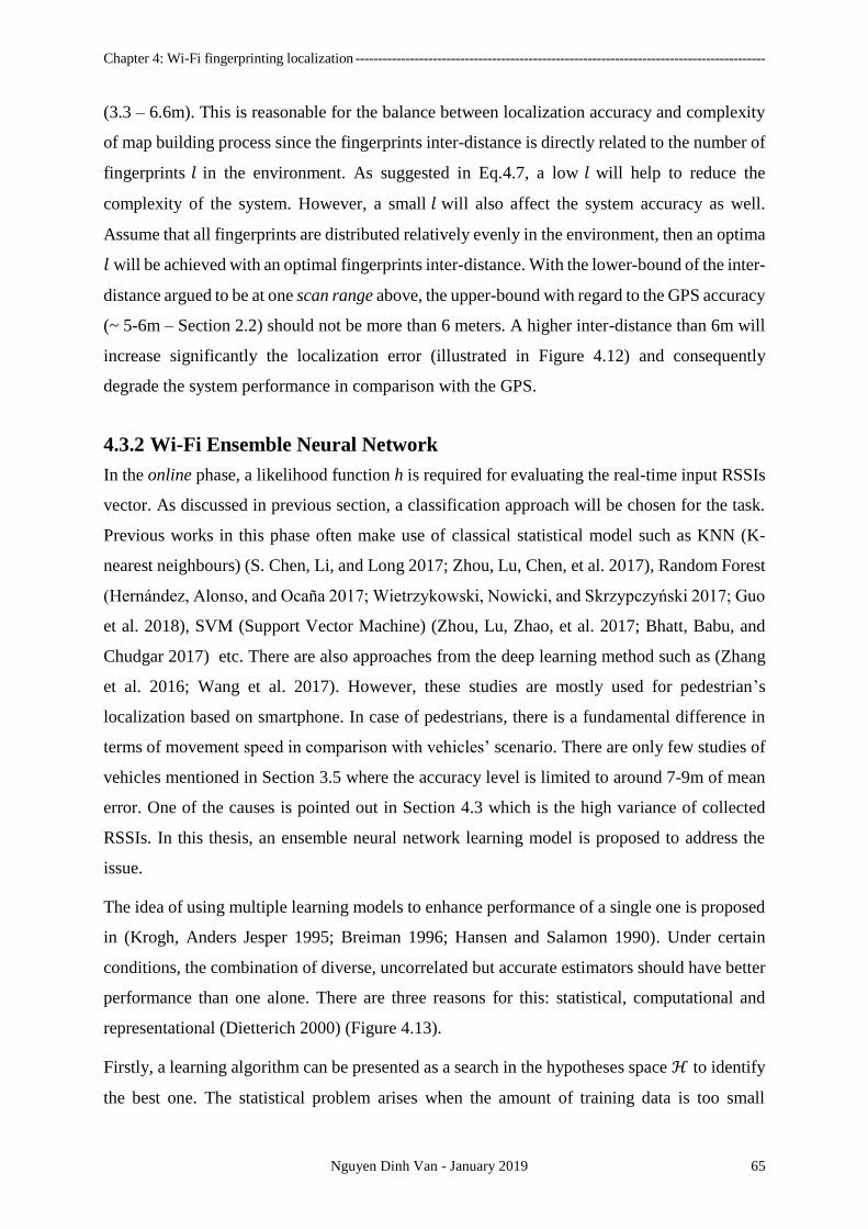
Chapter 4: Wi-Fi fingerprinting localization ------------------------------------------------------------------------------------------
Nguyen Dinh Van - January 2019 65
(3.3 – 6.6m). This is reasonable for the balance between localization accuracy and complexity
of map building process since the fingerprints inter-distance is directly related to the number of
fingerprints 𝑙 in the environment. As suggested in Eq.4.7, a low 𝑙 will help to reduce the
complexity of the system. However, a small 𝑙 will also affect the system accuracy as well.
Assume that all fingerprints are distributed relatively evenly in the environment, then an optima
𝑙 will be achieved with an optimal fingerprints inter-distance. With the lower-bound of the inter-
distance argued to be at one scan range above, the upper-bound with regard to the GPS accuracy
(~ 5-6m – Section 2.2) should not be more than 6 meters. A higher inter-distance than 6m will
increase significantly the localization error (illustrated in Figure 4.12) and consequently
degrade the system performance in comparison with the GPS.
4.3.2 Wi-Fi Ensemble Neural Network
In the online phase, a likelihood function h is required for evaluating the real-time input RSSIs
vector. As discussed in previous section, a classification approach will be chosen for the task.
Previous works in this phase often make use of classical statistical model such as KNN (K-
nearest neighbours) (S. Chen, Li, and Long 2017; Zhou, Lu, Chen, et al. 2017), Random Forest
(Hernández, Alonso, and Ocaña 2017; Wietrzykowski, Nowicki, and Skrzypczyński 2017; Guo
et al. 2018), SVM (Support Vector Machine) (Zhou, Lu, Zhao, et al. 2017; Bhatt, Babu, and
Chudgar 2017) etc. There are also approaches from the deep learning method such as (Zhang
et al. 2016; Wang et al. 2017). However, these studies are mostly used for pedestrian’s
localization based on smartphone. In case of pedestrians, there is a fundamental difference in
terms of movement speed in comparison with vehicles’ scenario. There are only few studies of
vehicles mentioned in Section 3.5 where the accuracy level is limited to around 7-9m of mean
error. One of the causes is pointed out in Section 4.3 which is the high variance of collected
RSSIs. In this thesis, an ensemble neural network learning model is proposed to address the
issue.
The idea of using multiple learning models to enhance performance of a single one is proposed
in (Krogh, Anders Jesper 1995; Breiman 1996; Hansen and Salamon 1990). Under certain
conditions, the combination of diverse, uncorrelated but accurate estimators should have better
performance than one alone. There are three reasons for this: statistical, computational and
representational (Dietterich 2000) (Figure 4.13).
Firstly, a learning algorithm can be presented as a search in the hypotheses space ℋ to identify
the best one. The statistical problem arises when the amount of training data is too small

Chapter 4: Wi-Fi fingerprinting localization ------------------------------------------------------------------------------------------
Nguyen Dinh Van - January 2019 66
compared to the size of ℋ. This is usually true in real life as it is impossible to cover all
hypotheses of a Wi-Fi fingerprinting problem. Without sufficient data, the learning algorithm
can find many different hypotheses with the same level of accuracy. By aggregating different,
uncorrelated good estimators, it reduces the risk of choosing a “wrong” one. Assume f in Figure
4.13 is the true hypothesis and in statistical case, h1, h2, h3 and h4 are equally good estimators.
An aggregation of those four may deliver a closer result to f than any of them.
Secondly, many learning algorithms suffer from local optimal which means that instead of
finding a global optimal solution, it may get stuck in a local one. Assume that there are sufficient
training data to cover most of ℋ , it is still very difficult to find a global optimal point
computationally. Building multiple estimators from different starting locations in hypotheses
space ℋ may provide a better approximation of the true optimal solution. In Figure 4.13 of
computational case, suppose h1, h2 and h3 are three estimators with different starting points in
the hypotheses space. Having a random start, each of those estimators will converge at a
different accuracy level. With a finite large number of estimators, there is a high possibility that
some of them overcome the local optimal point. Thus an ensemble of those estimators should
be more accurate than picking just one of them.
Finally, in many applications of machine learning, the true approximation function h cannot be
represented by any of the hypothesis in ℋ. This is also true in case of Wi-Fi fingerprinting as
the mapping h(X) = 𝐹𝑃 is impossible to model with a finite training samples. Thus, by taking
weighted sum of all estimators, it is possible that the outcome of the ensemble is closer to the
true answer. In Figure 4.13, the hypotheses space does not cover the true answer f. More often,
this is because of only a finite number of training data is collected. By aggregating h1, h2 and
h3, it is possible that the output accuracy is enhanced.
A necessary and sufficient condition for an ensemble estimator to be more accurate than any of
its individual is each individual estimator should be accurate and diverse (Hansen and Salamon
1990). An accurate estimator is the one that has an accuracy rate better than a random guessing
on new input value. Two estimators are diverse if they make different errors on new data. Thus,
in order to construct an ensemble of neural network, the thesis proposes to employ a bagging
technique (Bootstrap Aggregating) (Breiman 1996). The formal explanation of applying this
technique for ensemble neural network is following.
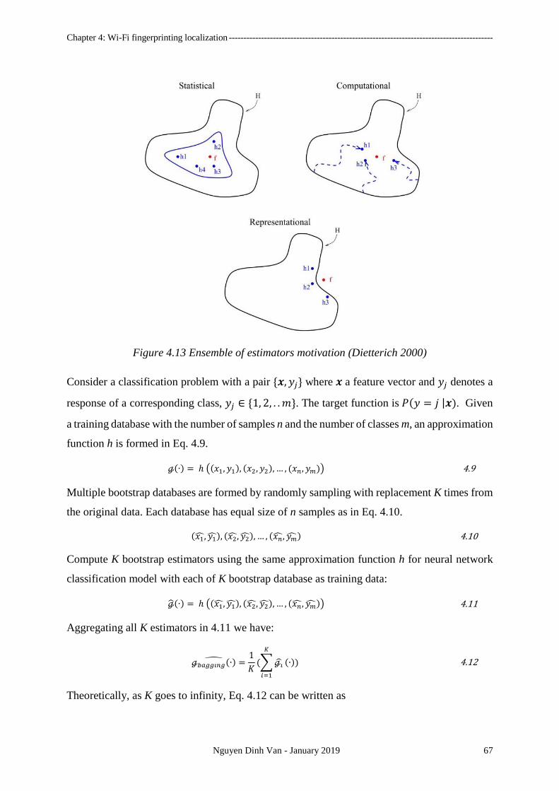
Chapter 4: Wi-Fi fingerprinting localization ------------------------------------------------------------------------------------------
Nguyen Dinh Van - January 2019 67
Figure 4.13 Ensemble of estimators motivation (Dietterich 2000)
Consider a classification problem with a pair 𝒙, 𝑦𝑗 where 𝒙 a feature vector and 𝑦𝑗 denotes a
response of a corresponding class, 𝑦𝑗 ∈ 1, 2, . . 𝑚. The target function is 𝑃(𝑦 = 𝑗 |𝒙). Given
a training database with the number of samples n and the number of classes m, an approximation
function h is formed in Eq. 4.9.
ℊ(∙) = ℎ ((𝑥1, 𝑦1), (𝑥2, 𝑦2), … , (𝑥𝑛 , 𝑦𝑚)) 4.9
Multiple bootstrap databases are formed by randomly sampling with replacement K times from
the original data. Each database has equal size of n samples as in Eq. 4.10.
(𝑥1, 𝑦1), (𝑥2, 𝑦2), … , (𝑥 , 𝑦) 4.10
Compute K bootstrap estimators using the same approximation function h for neural network
classification model with each of K bootstrap database as training data:
ℊ(∙) = ℎ ((𝑥1, 𝑦1), (𝑥2, 𝑦2), … , (𝑥 , 𝑦)) 4.11
Aggregating all K estimators in 4.11 we have:
ℊ𝑏𝑎𝑔𝑔𝑖𝑛𝑔(∙) =1
𝐾(∑ℊ
𝐾
𝑖=1
(∙)) 4.12
Theoretically, as K goes to infinity, Eq. 4.12 can be written as

Chapter 4: Wi-Fi fingerprinting localization ------------------------------------------------------------------------------------------
Nguyen Dinh Van - January 2019 68
ℊ𝑏𝑎𝑔𝑔𝑖𝑛𝑔(∙) = 𝑬[ℊ(∙)] 4.13
In practice, with a finite large K, the bagging estimator should come close to the expected global
optimal.
With the strategy for ensemble, it is now important to discuss the structure of an individual
neural network. A general fully connected architecture of a neural network with one hidden
layer is shown in Figure 4.14. The number of inputs nIn is determined by the size of the feature
vector 𝒙. Here, the feature vector should have the size of total learned MAC address in the
offline phase. Each neuron in the output layer is corresponding to a fingerprint. Thus, the
number of outputs nOut is the number of chosen fingerprints in the environment. The number
of neurons in the hidden layer, however, has no indicator. A two-third rule mentioned in
(Heaton 2008) is applied as in Eq, 4.14. The network weight is randomly initialized within
range of [0,1).
𝑛𝐻𝑖𝑑𝑑𝑒𝑛 =2
3(𝑛𝐼𝑛 + 𝑛𝑂𝑢𝑡) 4.14
A soft-max activation function is employed for the classification task of the network. The
general form of a soft-max activation function is:
𝑃(𝑦 = 𝑗 | 𝒙) = 𝑒𝑥
𝑇𝑤𝑗
∑ 𝑒𝑥𝑇𝑤𝑖𝑛
𝑖=1
4.15
Where wj is the weight of corresponding input in 𝐱.
Input Layer Hidden Layer Output Layer
nOut = 𝑙
nHidden
nIn = v
Figure 4.14 Fully connected neural network with 1 hidden layer
In case of Wi-Fi fingerprinting localization for intelligent vehicles, given the hybrid database
proposed above, a bootstrap database is explained as in Figure 4.15. By randomly select with
replacement each row of the original hybrid database, a new bootstrap database is constructed.
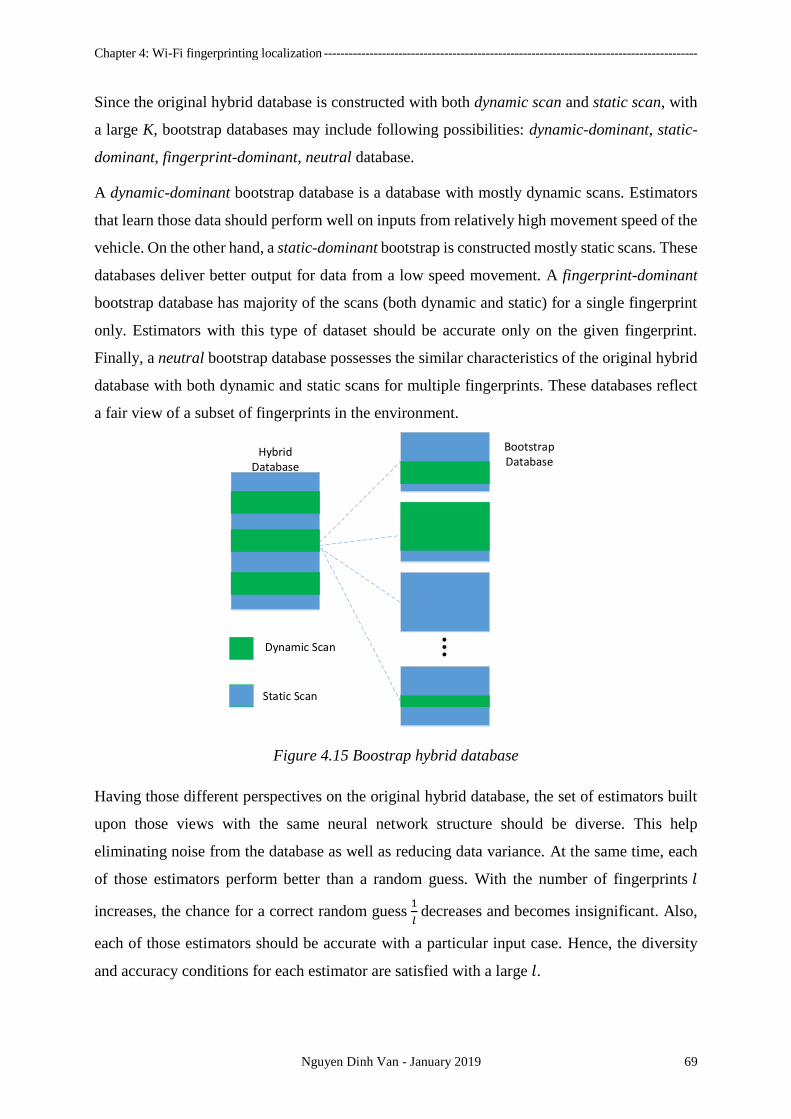
Chapter 4: Wi-Fi fingerprinting localization ------------------------------------------------------------------------------------------
Nguyen Dinh Van - January 2019 69
Since the original hybrid database is constructed with both dynamic scan and static scan, with
a large K, bootstrap databases may include following possibilities: dynamic-dominant, static-
dominant, fingerprint-dominant, neutral database.
A dynamic-dominant bootstrap database is a database with mostly dynamic scans. Estimators
that learn those data should perform well on inputs from relatively high movement speed of the
vehicle. On the other hand, a static-dominant bootstrap is constructed mostly static scans. These
databases deliver better output for data from a low speed movement. A fingerprint-dominant
bootstrap database has majority of the scans (both dynamic and static) for a single fingerprint
only. Estimators with this type of dataset should be accurate only on the given fingerprint.
Finally, a neutral bootstrap database possesses the similar characteristics of the original hybrid
database with both dynamic and static scans for multiple fingerprints. These databases reflect
a fair view of a subset of fingerprints in the environment.
Dynamic Scan
Static Scan
Hybrid Database
Bootstrap Database
Figure 4.15 Boostrap hybrid database
Having those different perspectives on the original hybrid database, the set of estimators built
upon those views with the same neural network structure should be diverse. This help
eliminating noise from the database as well as reducing data variance. At the same time, each
of those estimators perform better than a random guess. With the number of fingerprints 𝑙
increases, the chance for a correct random guess 1
𝑙 decreases and becomes insignificant. Also,
each of those estimators should be accurate with a particular input case. Hence, the diversity
and accuracy conditions for each estimator are satisfied with a large 𝑙.
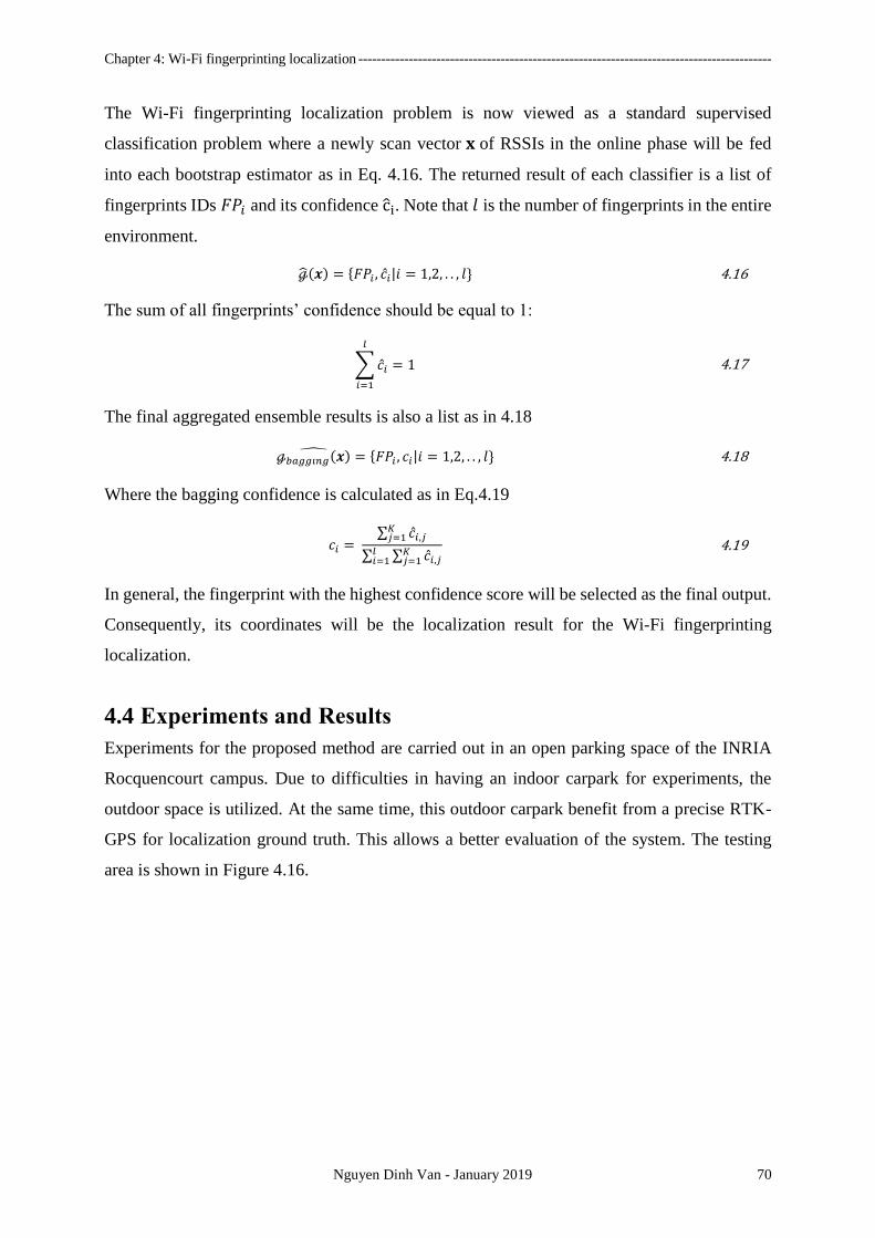
Chapter 4: Wi-Fi fingerprinting localization ------------------------------------------------------------------------------------------
Nguyen Dinh Van - January 2019 70
The Wi-Fi fingerprinting localization problem is now viewed as a standard supervised
classification problem where a newly scan vector 𝐱 of RSSIs in the online phase will be fed
into each bootstrap estimator as in Eq. 4.16. The returned result of each classifier is a list of
fingerprints IDs 𝐹𝑃𝑖 and its confidence c i. Note that 𝑙 is the number of fingerprints in the entire
environment.
ℊ(𝒙) = 𝐹𝑃𝑖 , 𝑐 𝑖|𝑖 = 1,2, . . , 𝑙 4.16
The sum of all fingerprints’ confidence should be equal to 1:
∑𝑐 𝑖
𝑙
𝑖=1
= 1 4.17
The final aggregated ensemble results is also a list as in 4.18
ℊ𝑏𝑎𝑔𝑔𝑖𝑛𝑔(𝒙) = 𝐹𝑃𝑖 , 𝑐𝑖|𝑖 = 1,2, . . , 𝑙 4.18
Where the bagging confidence is calculated as in Eq.4.19
𝑐𝑖 = ∑ 𝑐 𝑖,𝑗𝐾𝑗=1
∑ ∑ 𝑐 𝑖,𝑗𝐾𝑗=1
𝑙𝑖=1
4.19
In general, the fingerprint with the highest confidence score will be selected as the final output.
Consequently, its coordinates will be the localization result for the Wi-Fi fingerprinting
localization.
4.4 Experiments and Results
Experiments for the proposed method are carried out in an open parking space of the INRIA
Rocquencourt campus. Due to difficulties in having an indoor carpark for experiments, the
outdoor space is utilized. At the same time, this outdoor carpark benefit from a precise RTK-
GPS for localization ground truth. This allows a better evaluation of the system. The testing
area is shown in Figure 4.16.

Chapter 4: Wi-Fi fingerprinting localization ------------------------------------------------------------------------------------------
Nguyen Dinh Van - January 2019 71
Figure 4.16 Testing area in INRIA Rocquencourt campus
There are two vehicles in the experiments: a blue Cybercar designed as a prototype for
intelligent vehicles and a red Citroen C1 with modification for experimental purposes. The two
vehicles are shown in Figure 4.17.
Figure 4.17 Blue Cybercar and Red Citroen C1
Both vehicles are equipped with a Wi-Fi receiver, a RTK-GPS receiver, an IMU system and
two LiDAR sensors (front and back). The average movement speed across all experiments is
around 2.5m/s to 3.0m/s.
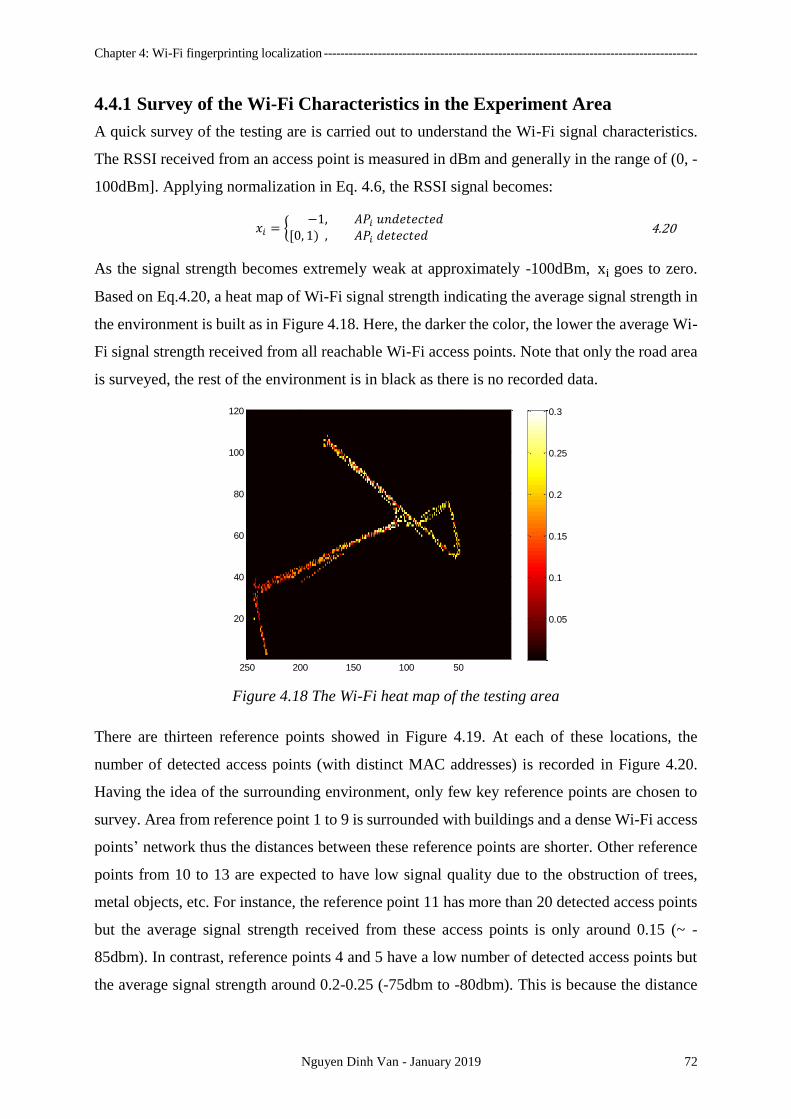
Chapter 4: Wi-Fi fingerprinting localization ------------------------------------------------------------------------------------------
Nguyen Dinh Van - January 2019 72
4.4.1 Survey of the Wi-Fi Characteristics in the Experiment Area
A quick survey of the testing are is carried out to understand the Wi-Fi signal characteristics.
The RSSI received from an access point is measured in dBm and generally in the range of (0, -
100dBm]. Applying normalization in Eq. 4.6, the RSSI signal becomes:
𝑥𝑖 = −1, 𝐴𝑃𝑖 𝑢𝑛𝑑𝑒𝑡𝑒𝑐𝑡𝑒𝑑
[0, 1) , 𝐴𝑃𝑖 𝑑𝑒𝑡𝑒𝑐𝑡𝑒𝑑 4.20
As the signal strength becomes extremely weak at approximately -100dBm, xi goes to zero.
Based on Eq.4.20, a heat map of Wi-Fi signal strength indicating the average signal strength in
the environment is built as in Figure 4.18. Here, the darker the color, the lower the average Wi-
Fi signal strength received from all reachable Wi-Fi access points. Note that only the road area
is surveyed, the rest of the environment is in black as there is no recorded data.
Figure 4.18 The Wi-Fi heat map of the testing area
There are thirteen reference points showed in Figure 4.19. At each of these locations, the
number of detected access points (with distinct MAC addresses) is recorded in Figure 4.20.
Having the idea of the surrounding environment, only few key reference points are chosen to
survey. Area from reference point 1 to 9 is surrounded with buildings and a dense Wi-Fi access
points’ network thus the distances between these reference points are shorter. Other reference
points from 10 to 13 are expected to have low signal quality due to the obstruction of trees,
metal objects, etc. For instance, the reference point 11 has more than 20 detected access points
but the average signal strength received from these access points is only around 0.15 (~ -
85dbm). In contrast, reference points 4 and 5 have a low number of detected access points but
the average signal strength around 0.2-0.25 (-75dbm to -80dbm). This is because the distance
50100150200250
20
40
60
80
100
120
0.05
0.1
0.15
0.2
0.25
0.3
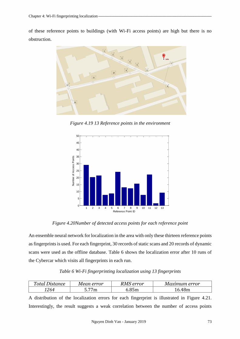
Chapter 4: Wi-Fi fingerprinting localization ------------------------------------------------------------------------------------------
Nguyen Dinh Van - January 2019 73
of these reference points to buildings (with Wi-Fi access points) are high but there is no
obstruction.
Figure 4.19 13 Reference points in the environment
Figure 4.20Number of detected access points for each reference point
An ensemble neural network for localization in the area with only these thirteen reference points
as fingerprints is used. For each fingerprint, 30 records of static scans and 20 records of dynamic
scans were used as the offline database. Table 6 shows the localization error after 10 runs of
the Cybercar which visits all fingerprints in each run.
Table 6 Wi-Fi fingerprinting localization using 13 fingerprints
Total Distance Mean error RMS error Maximum error
1264 5.77m 6.85m 16.48m
A distribution of the localization errors for each fingerprint is illustrated in Figure 4.21.
Interestingly, the result suggests a weak correlation between the number of access points
1
2
3
4
5
6
7
8
9
10
11
12
13
1 2 3 4 5 6 7 8 9 10 11 12 130
5
10
15
20
25
30
35
40
45
50
Reference Point ID
Num
ber
of
Access P
oin
ts
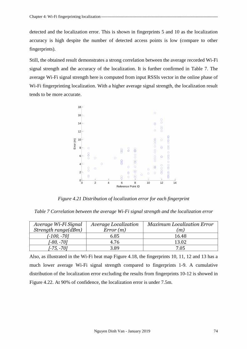
Chapter 4: Wi-Fi fingerprinting localization ------------------------------------------------------------------------------------------
Nguyen Dinh Van - January 2019 74
detected and the localization error. This is shown in fingerprints 5 and 10 as the localization
accuracy is high despite the number of detected access points is low (compare to other
fingerprints).
Still, the obtained result demonstrates a strong correlation between the average recorded Wi-Fi
signal strength and the accuracy of the localization. It is further confirmed in Table 7. The
average Wi-Fi signal strength here is computed from input RSSIs vector in the online phase of
Wi-Fi fingerprinting localization. With a higher average signal strength, the localization result
tends to be more accurate.
Figure 4.21 Distribution of localization error for each fingerprint
Table 7 Correlation between the average Wi-Fi signal strength and the localization error
Average Wi-Fi Signal Strength range(dBm)
Average Localization Error (m)
Maximum Localization Error (m)
(-100, -70] 6.85 16.48 [-80, -70] 4.76 13.02 [-75, -70] 3.89 7.05
Also, as illustrated in the Wi-Fi heat map Figure 4.18, the fingerprints 10, 11, 12 and 13 has a
much lower average Wi-Fi signal strength compared to fingerprints 1-9. A cumulative
distribution of the localization error excluding the results from fingerprints 10-12 is showed in
Figure 4.22. At 90% of confidence, the localization error is under 7.5m.
0 2 4 6 8 10 12 140
2
4
6
8
10
12
14
16
18
Reference Point ID
Err
or
(m)
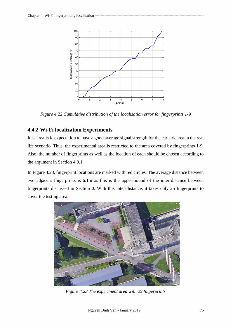
Chapter 4: Wi-Fi fingerprinting localization ------------------------------------------------------------------------------------------
Nguyen Dinh Van - January 2019 75
Figure 4.22 Cumulative distribution of the localization error for fingerprints 1-9
4.4.2 Wi-Fi localization Experiments
It is a realistic expectation to have a good average signal strength for the carpark area in the real
life scenario. Thus, the experimental area is restricted to the area covered by fingerprints 1-9.
Also, the number of fingerprints as well as the location of each should be chosen according to
the argument in Section 4.3.1.
In Figure 4.23, fingerprint locations are marked with red circles. The average distance between
two adjacent fingerprints is 6.1m as this is the upper-bound of the inter-distance between
fingerprints discussed in Section 0. With this inter-distance, it takes only 25 fingerprints to
cover the testing area.
Figure 4.23 The experiment area with 25 fingerprints
0 1 2 3 4 5 6 7 80
10
20
30
40
50
60
70
80
90
100
Eror (m)
Cum
ula
tive P
erc
enta
ge %

Chapter 4: Wi-Fi fingerprinting localization ------------------------------------------------------------------------------------------
Nguyen Dinh Van - January 2019 76
For each fingerprint, 60 static scans and 20 dynamic scans are recorded for the offline database.
A total 156 access points with different MAC addresses are detected across 25 fingerprints. By
apply the rule in Eq.4.14, an individual neural network in the ensemble has the architecture as
following:
nIn = 156; nOut = 25; nHidden = 120 4.21
The number of individual neural networks is K = 50. For each network, a 10 random early-
restarts in the training phase (Magdon-Ismail and Atiya 2000; Prechelt 2012) is applied in order
to avoid local optimum.
A 10-fold cross-validation test with 80% data for the training set, 10% data for the validation
set and 10% data for the test set is performed on the neural network structure with the hybrid
training database. The average cross-entropy error is low at 0.428 which indicates a good
generalization error of the network architecture.
One of the major issues with this classification approach is that in real life, there are inputs
which do not match with any specific class (i.e a RSSIs vector collected in between two adjacent
fingerprints). Theoretically, these inputs should not be classified into any class. However, as
the Wi-Fi fingerprinting localization acts as a global level of localization system, it should give
a good indication of absolute positioning of the vehicle. Thus, we then define a good
classification result of the neural network as the closest fingerprints to the ground truth in
Euclidean distance. As mentioned in Eq. 4.18, result from the Ensemble Neural Network is a
list of fingerprints’ indices and their corresponding confidence. Assume that the highest
confidence fingerprint is chosen as the final classification result, it is a good classification result
if:
𝑑𝑖𝑠𝑡(𝐹𝑃𝑐_𝑚𝑎𝑥 , 𝐺𝑟𝑜𝑢𝑛𝑑 𝑇𝑟𝑢𝑡ℎ) = 𝑚𝑖𝑛 𝑑𝑖𝑠𝑡(𝐹𝑃𝑖 , 𝐺𝑟𝑜𝑢𝑛𝑑 𝑇𝑟𝑢𝑡ℎ) 4.22
Here dist is the Euclidean distance function. Similarly, all other fingerprints can be examined.
Table 8 shows the statistical of good classification rate if classification result is chosen from
top 3 highest confidence fingerprints. Those results are obtained from 64 test runs in one year
period with 9058 classification estimation.
In the classification approach for Wi-Fi fingerprinting localization, the fingerprint with the
highest confidence score will be selected as the localization result. However, based on the
statistic above, a threshold 𝜃 for the confidence score is set. The fingerprint with the highest
confidence score is selected as the final result if only Eq.4.23 is satisfied.
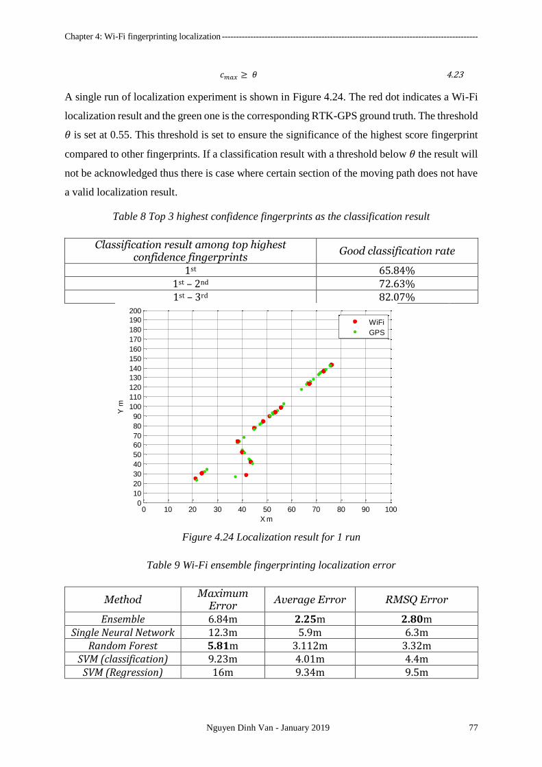
Chapter 4: Wi-Fi fingerprinting localization ------------------------------------------------------------------------------------------
Nguyen Dinh Van - January 2019 77
𝑐𝑚𝑎𝑥 ≥ 𝜃 4.23
A single run of localization experiment is shown in Figure 4.24. The red dot indicates a Wi-Fi
localization result and the green one is the corresponding RTK-GPS ground truth. The threshold
𝜃 is set at 0.55. This threshold is set to ensure the significance of the highest score fingerprint
compared to other fingerprints. If a classification result with a threshold below 𝜃 the result will
not be acknowledged thus there is case where certain section of the moving path does not have
a valid localization result.
Table 8 Top 3 highest confidence fingerprints as the classification result
Classification result among top highest confidence fingerprints
Good classification rate
1st 65.84% 1st – 2nd 72.63% 1st – 3rd 82.07%
Figure 4.24 Localization result for 1 run
Table 9 Wi-Fi ensemble fingerprinting localization error
Method Maximum
Error Average Error RMSQ Error
Ensemble 6.84m 2.25m 2.80m Single Neural Network 12.3m 5.9m 6.3m
Random Forest 5.81m 3.112m 3.32m SVM (classification) 9.23m 4.01m 4.4m
SVM (Regression) 16m 9.34m 9.5m
0 10 20 30 40 50 60 70 80 90 1000
10
20
30
40
50
60
70
80
90
100
110
120
130
140
150
160
170
180
190
200
X m
Y m
WiFi
GPS

Chapter 4: Wi-Fi fingerprinting localization ------------------------------------------------------------------------------------------
Nguyen Dinh Van - January 2019 78
A quick comparison of the Wi-Fi ensemble fingerprinting localization with other methods such
as random forest, SVM, and Single Neural Network can be seen in Table 9. An improvement
is observed compared to the survey results presented in previous section. With maximum error
at 6.84m and average error of 2.25m, the performance of the Wi-Fi ensemble fingerprinting
localization is equivalence to the performance of standard GPS mentioned in Table 1. Although
a better maximum error is found in the random forest approach, ensemble method delivers a
much better average localization error. Note that the random forest used in the experiment has
50 sub-trees which is equal to the number of individual neural networks in the ensemble
method.
4.5 Discussion
This chapter presents a novel method of Wi-Fi fingerprinting localization using Ensemble
Neural network for intelligent vehicles. To the best of the author knowledge, this is the first
solution for localizing an intelligent vehicle using Wi-Fi signals. Other approaches are either
for human walking or industrial robots. The only recent solution which applies for intelligent
vehicle is mentioned in (Hernandez et al. 2017) has a much lower accuracy at 9.34m of average
localization error.
Having defined the original Wi-Fi fingerprinting localization method, two significant changes
are proposed in this thesis: an offline hybrid database and an online ensemble neural network
for classification.
As discussed in Section 4.3.1, while the target of localization is moving, it is not always possible
to characterize a fingerprint as one single position in the environment. In fact, depending on the
target’s movement speed, the distance that it moves to complete a Wi-Fi scan varies. This
distance, defined as a scan range, has a critical impact on the offline phase map building
complexity as well as the accuracy of the online phase localization. Based on the average
movement speed of a car in a car park, this thesis defines a hybrid database with both dynamic
and static fingerprints. Compared to the traditional static databases of fingerprints, this hybrid
database is supposed to represent better the characteristics of the moving vehicle in a real life
situation. This is justified in the improved localization accuracy from experiments with average
error at only 2.25m. In addition, the author also discusses the optimal range for the inter-
distance between two consecutive fingerprints in the environment. For a balance between
complexity and accuracy of the problem, an inter-distance range from one scan range to two
scan ranges is believed to be optimal.

Chapter 4: Wi-Fi fingerprinting localization ------------------------------------------------------------------------------------------
Nguyen Dinh Van - January 2019 79
Together with the hybrid database, an ensemble neural network is proposed to solve the
problem of high variance and high noise in the Wi-Fi signal strength collecting process. At the
start of this thesis, a thorough search of the relevant literature did not yield any significant study
that uses the method for the Wi-Fi fingerprinting localization. Only recently studies from
(Torres-Sospedra et al. 2016; Ta et al. 2016) which embrace the ensemble strategy for the Wi-
Fi fingerprinting are found. These studies achieve a significant boost in accuracy of 3.39m for
localization. However, these are studies for human localization using smartphone which has
two fundamental differences with the vehicle localization problem: movement speed and
hardware consistency. If the movement speed of a human is expected to be much lower than a
vehicle, then the hardware (more specifically the Wi-Fi antenna) of a smartphone has a much
lower consistency than a dedicated Wi-Fi antenna for a vehicle. Hence, it is difficult to make a
direct comparison between the Wi-Fi fingerprinting localization performance for human using
a smartphone and intelligent vehicles using a dedicated antenna. Therefore, in Section 4.3.2,
the ensemble method is presented only for intelligent vehicles localization case using the hybrid
database which is mentioned previously. A quick comparison with other solutions such as
Random Forest, single neural network, SVM classification or SVM regression (Hernandez et
al. 2017) shows that the ensemble neural network with hybrid database provides a higher
accuracy than the other approaches.
With the fingerprints’ coordinates measured in global coordinate framework (WGS84
standard), this solution can be directly compared to the outdoor performance of the Global
Positioning System (GPS). With only 2.25m of average error, in an environment with high
density and quality of Wi-Fi signals, this solution out-performs the GPS. Naturally, this is also
true for the GPS-denied area. Hence, the Wi-Fi fingerprinting localization can provide a smooth
transition for global localization from GPS-aided area to GPS-denied area.
Finally, with the Wi-Fi system is often readily available, this solution can be deployed quickly
in urban area such as car park. Also, the mapping phase of the Wi-Fi fingerprinting localization
is much simpler at low cost compared to other methods such as camera-based or Lidar-based.
This is achieved because instead of building a continuous detailed map of the environment, the
Wi-Fi fingerprinting localization system creates a discrete map of fingerprints to represent the
environment. The characteristic benefits both the initial deployment process and the map
correction later on.

Chapter 4: Wi-Fi fingerprinting localization ------------------------------------------------------------------------------------------
Nguyen Dinh Van - January 2019 80
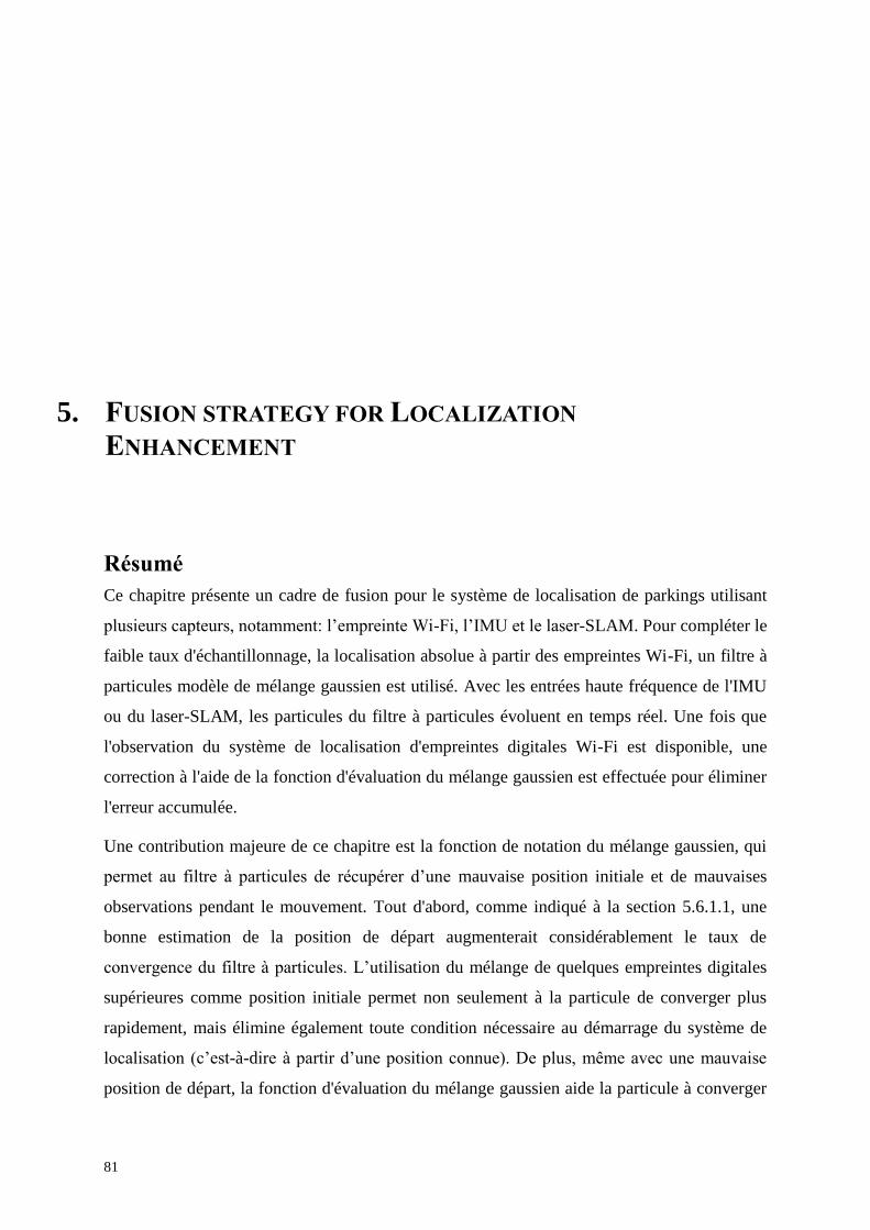
81
5. FUSION STRATEGY FOR LOCALIZATION
ENHANCEMENT
Résumé
Ce chapitre présente un cadre de fusion pour le système de localisation de parkings utilisant
plusieurs capteurs, notamment: l’empreinte Wi-Fi, l’IMU et le laser-SLAM. Pour compléter le
faible taux d'échantillonnage, la localisation absolue à partir des empreintes Wi-Fi, un filtre à
particules modèle de mélange gaussien est utilisé. Avec les entrées haute fréquence de l'IMU
ou du laser-SLAM, les particules du filtre à particules évoluent en temps réel. Une fois que
l'observation du système de localisation d'empreintes digitales Wi-Fi est disponible, une
correction à l'aide de la fonction d'évaluation du mélange gaussien est effectuée pour éliminer
l'erreur accumulée.
Une contribution majeure de ce chapitre est la fonction de notation du mélange gaussien, qui
permet au filtre à particules de récupérer d’une mauvaise position initiale et de mauvaises
observations pendant le mouvement. Tout d'abord, comme indiqué à la section 5.6.1.1, une
bonne estimation de la position de départ augmenterait considérablement le taux de
convergence du filtre à particules. L’utilisation du mélange de quelques empreintes digitales
supérieures comme position initiale permet non seulement à la particule de converger plus
rapidement, mais élimine également toute condition nécessaire au démarrage du système de
localisation (c’est-à-dire à partir d’une position connue). De plus, même avec une mauvaise
position de départ, la fonction d'évaluation du mélange gaussien aide la particule à converger

Chapter 5: Fusion strategy for Localization Enhancement -------------------------------------------------------------------------
Nguyen Dinh Van - January 2019 82
rapidement. Ceci est montré dans les résultats d'expériences de cas de test où la position initiale
est en dehors de la zone d'empreinte digitale. L'erreur de localisation est rapidement réduite
lorsque le véhicule se rapproche d'une empreinte digitale. Deuxièmement, les observations du
système de localisation d'empreintes digitales Wi-Fi ne donnent pas toujours une bonne
estimation de la position réelle. Au lieu de cela, il s'agit d'un cas de test réel présenté dans la
section 5.3.2, dans lequel le résultat de classification de confiance le plus élevé de la localisation
d'empreintes digitales Wi-Fi n'est pas un bon résultat de classification. Cependant, la fonction
de notation du modèle de mélange gaussien donne au filtre à particules une chance de surmonter
une telle situation en prenant en compte les autres résultats de classification supérieurs qui
devraient théoriquement rapprocher l'estimation de la position réelle.
Une autre proposition intéressante de ce chapitre concerne la stratégie visant à fusionner le
SLAM laser en un système de coordonnées global sans recourir à un processus d'initialisation
ou à une carte laser prédéfinie. Contrairement aux autres solutions mentionnées au chapitre 2,
ce framework de fusion ne nécessite pas de position initiale soigneusement calibrée pour le
SLAM laser ni de carte prédéfinie pour la formulation d'une matrice de transformation entre la
coordonnée SLAM et la coordonnée globale. Au lieu de cela, tirant parti de la haute précision
du SLAM dans l’estimation par pas local, le cadre de fusion incorpore le laser-SLAM en tant
qu’IMU, ce qui réduit le besoin d’une matrice de transformation.
Au cours d'une année d'expériences, la fusion de la localisation des empreintes digitales IMU
et Wi-Fi est testée avec différents critères tels que: la stabilité du filtre à particules, le nombre
de particules et le comportement du système avec différentes positions de départ.
Pour comprendre la stabilité du filtre à particules conçu, le système de fusion est testé sous deux
perspectives: plusieurs exécutions sur le même jeu de données et différents jeux de données.
Dans la première perspective, un seul jeu de données est introduit indépendamment dans
l'algorithme pour 100 itérations. L'erreur de localisation moyenne et son écart type sont calculés
au-dessus des 100 itérations. Une erreur moyenne faible (environ 0,8 m dans tous les cas et 0,5
m pour une bonne position de départ), ainsi qu'un faible écart type (~ 0,22) indiquent que le
filtre à particules est stable. Pour la deuxième perspective, un total de 84 expériences
indépendantes ont été menées. Les résultats finaux donnent un résultat similaire avec une erreur
moyenne et un écart type de 0,859 m et 0,232 pour tous les cas et de 0,588 m et 0,127 pour une
bonne position initiale. Ainsi, il a été prouvé que le filtre à particules conçu est stable.
Chapter 5: Fusion strategy for Localization Enhancement -------------------------------------------------------------------------
Nguyen Dinh Van - January 2019 83
Le nombre de particules dans un filtre à particules (ou sa dimension) est également un paramètre
important. Cela détermine les ressources nécessaires pour que l'algorithme s'exécute en temps
réel. Pour apprendre ce paramètre, différents nombres de particules sont testés dans le même
jeu de données. Enfin, avec seulement 2000 particules, la solution de fusion est capable
d’obtenir un résultat optimal.
Différentes positions initiales pour les tests sont également étudiées pour comprendre la
généralisation de l’algorithme. Il existe deux possibilités de lieu pour la position initiale: à
l'intérieur ou à l'extérieur d'une zone d'empreinte digitale. Si la position initiale est dans une
zone d'empreinte digitale, une bonne estimation initiale peut être attendue. Cela se traduit par
une faible erreur de localisation moyenne de 0,588 m. Sinon, comme le filtre à particules a
besoin de temps pour converger vers la position vraie, l'erreur de localisation moyenne dans ce
cas est d'environ 0,859 m. Cette erreur moyenne élevée est principalement due à la grande erreur
de positionnement initiale. En outre, il est raisonnable de s’attendre à ce que la position initiale
d’un véhicule entrant dans un parc de stationnement soit relativement connue. Par conséquent,
une bonne précision peut être attendue du système de fusion en général.
Bien que la vitesse de déplacement moyenne dans toutes les expériences soit d'environ 3,3 m /
s, il est possible d'étendre le résultat de la thèse à une vitesse de déplacement supérieure. Pour
ce faire, il faut trouver une solution permettant d’améliorer la fréquence d’échantillonnage de
localisation des empreintes digitales Wi-Fi. Une solution potentielle consiste à utiliser plusieurs
antennes Wi-Fi avec différents processeurs, chacun ayant un léger retard par rapport à l'autre.
De cette manière, la fréquence d'échantillonnage du balayage Wi-Fi peut être augmentée
proportionnellement au nombre d'antennes. Malheureusement, avec un temps limité, la thèse
n'a pas pu être étendue pour couvrir l'idée.
Enfin, le cadre de fusion proposé permet non seulement de fusionner les empreintes Wi-Fi avec
d’autres capteurs, mais il est également possible de combiner différentes stratégies telles que le
GPS avec SLAM laser, le GPS avec système de localisation par caméra, etc. Cela étant dit, ce
cadre peut être appliqué à plusieurs scénarios, mais pas uniquement à un sans GPS
environnement ou à un parking privé.
5.1 Introduction
Up to this section, a global localization strategy for intelligent vehicles using Wi-Fi is presented.
Chapter 4 proves that the Wi-Fi fingerprinting localization is capable of matching the standard
GPS performance. However, at around 1Hz of sampling rate, both the Wi-Fi fingerprinting
Chapter 5: Fusion strategy for Localization Enhancement -------------------------------------------------------------------------
Nguyen Dinh Van - January 2019 84
system and the standard GPS are failing to track a moving vehicle at a relatively high speed.
This problem is commonly solved by integrating other sources of location estimation into the
system to smoothly increase the sampling rate as well as the positioning accuracy (N. E. El
Faouzi, Leung, and Kurian 2011).
In fact, almost all localization systems are fusion systems of different sensors. For instance,
approaches in (Carlson, Thorpe, and Browning 2010; Kim 2004; Amini et al. 2014; Schleicher
et al. 2009) integrate the GPS absolute localization measurements into camera, laser or dead-
reckoning localization system. These methods use the same tactics discussed in Chapter 2, with
the GPS giving a raw global estimation while other sensors such as laser, camera, IMU, etc.
offer local positioning. Results from the GPS and other sensors must be expressed in the same
coordinate system to infer the final localization result. These methods often require an
initialization process to find the transformation matrix between the sensors local coordinates
system and the global one of the GPS.
Compare to a single sensor approach, a multiple sensors fusion localization system has
advantages in terms of coverage range, adaptation and redundancy. Each sensor has a different
coverage range. A laser sensor has the maximum measurement range from 20m up to 200m
while most of cameras should have around 20-30m of effective range. In addition, under
different environment conditions, sensors may not function properly. While the lighting
conditions of the environment rarely influence the laser measurement accuracy, it has a major
impact on the camera system performance. However, the camera system is superior when it
comes to landmarks or objects detection and identification. Similarly, the GPS is globally
accepted for the outdoor localization but is failed to perform in the indoor environment. Thus,
a well-designed fusion system should theoretically adapt well to changes of the environment
conditions (Kunz et al. 2015). Lastly, by having inputs from different sensor types, the system
offers redundancy. Since each sensor has its own advantages and disadvantages, the
combination of more than one sensor type’s information may help to overcome each one’s
limitation.
In localization problem, there are several algorithms dedicated to sensors fusion such as Kalman
filtering, grid-based Markov localization, Particle filtering or Neural Network etc. Those
approaches can be split into three categories: Statistic based, Probabilistic based and Machine
Learning based.

Chapter 5: Fusion strategy for Localization Enhancement -------------------------------------------------------------------------
Nguyen Dinh Van - January 2019 85
Statistical approaches often make use of weighted combination of sources. The weighting is
based on statistical analysis of a recorded dataset (Han, Kamber, and Pei 2012). However, these
approaches are not suitable when information from sensors are not exchangeable or when the
performance of sensors are vastly different (N.-E. El Faouzi 1997).
Probability approaches use a distribution model to estimate weight of data. Methods such as
Kalman filtering (Dongliang Huang and Leung 2004; Kalman 1960), Evidential theory
(Trehard et al. 2014; Shafer 1976) or Particle filtering (Daum, Huang, and Noushin 2011;
F.~Gustafsson 2010; Calvet, Czellar, and Ronchetti 2015) are some significant representatives
of the category. They are widely used in recent solutions for localization.
Machine Learning approaches are quickly becoming a new popular solution as well. With
algorithms such as neural networks, genetic algorithms and especially deep learning, these
approaches deliver promising results (Moreira et al. 2019; Abdallah, Saab, and Kassas 2018).
Those approaches rely on a huge database of training data to predict the true fusion parameters.
They are commonly found in cameras system or WSNs (Zhang et al. 2016; Belagiannis et al.
2015; Iter, Kuck, and Zhuang 2016).
Table 10 Comparison of Algorithms for Nonlinear Filtering (Daum 2005)
Extended Kalman
Filter
Unscented Kalman Filter
Particle Filter
Numerical Solution of
Fokker-Planck
Equation
Exact Nonlinear Recursive
Filter
Batch or Non-
recursive Filter
Statistics propagated
by the algorithm
Mean vector and
covariance matrix
Mean vector and covariance
matrix
Complete probability
density conditioned
on the measurement
Complete probability
density conditioned
on the measurement
Sufficient statistics
Mean vector and
covariance matrix
Prediction of statistics from one
measurement time to the
next
Linear approximatio
n of the measurement
equations
Approximation of the
multidimensional integrals using the
“unscented transformation”
Monte Carlo Integration
using importance
sampling
Finite difference or
other numerical solution of the Fokker-Planck PDE
Numerical integration of ODEs for
the sufficient statistic in
the exponential
family of probability
densities
Numerical integration
Correction of statistics at
measurement time
Linear approximatio
n of the measurement
equations
Approximation of the
multidimensional integrals using the
“unscented transformation”
Monte Carlo sampling of
the conditional
density using both
importance sampling & resampling
Bayes’ rule
Bayes’ rule for
exponential family of
probability densities
Numerical minimizatio
n of cost criterion
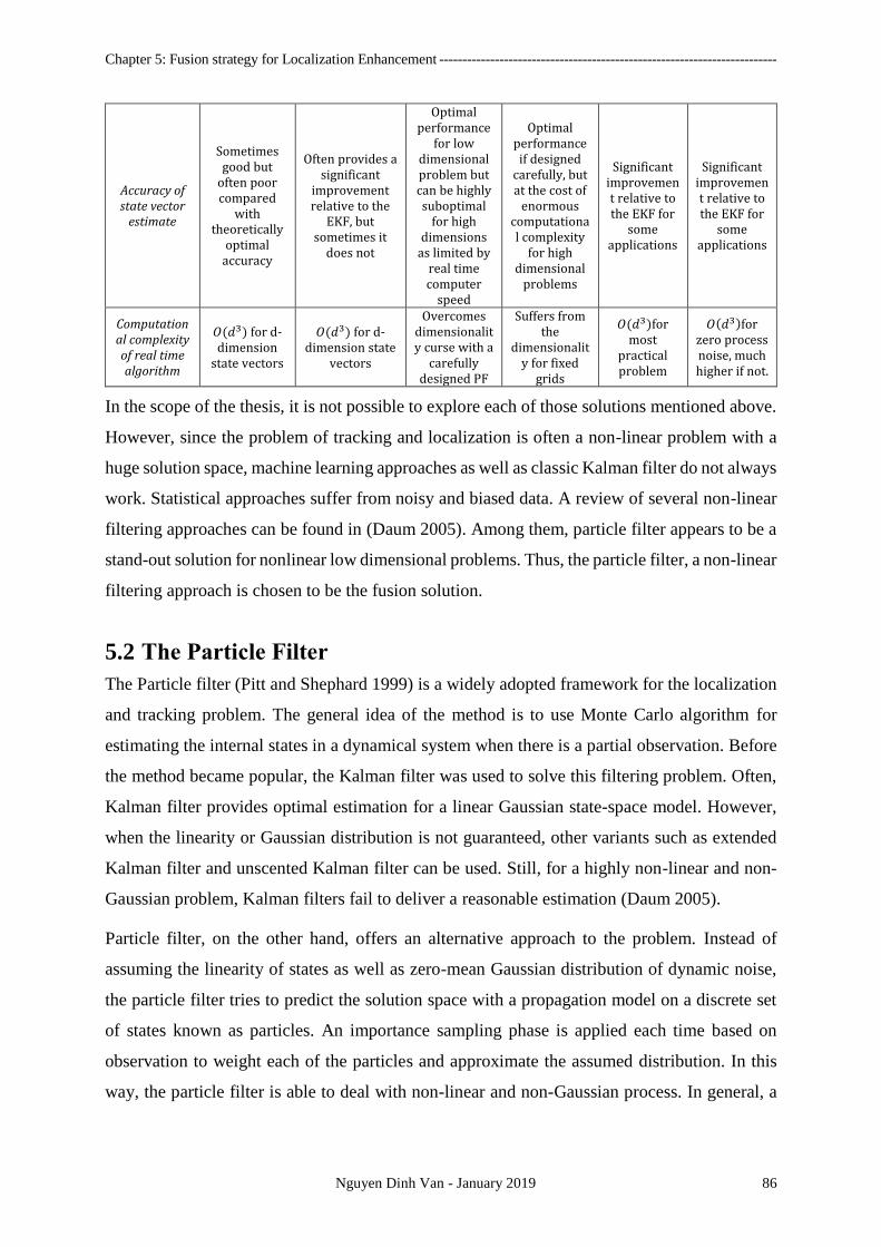
Chapter 5: Fusion strategy for Localization Enhancement -------------------------------------------------------------------------
Nguyen Dinh Van - January 2019 86
Accuracy of state vector
estimate
Sometimes good but
often poor compared
with theoretically
optimal accuracy
Often provides a significant
improvement relative to the
EKF, but sometimes it
does not
Optimal performance
for low dimensional problem but can be highly suboptimal
for high dimensions
as limited by real time computer
speed
Optimal performance if designed
carefully, but at the cost of
enormous computational complexity
for high dimensional
problems
Significant improvement relative to the EKF for
some applications
Significant improvement relative to the EKF for
some applications
Computational complexity of real time algorithm
𝑂(𝑑3) for d-dimension
state vectors
𝑂(𝑑3) for d-dimension state
vectors
Overcomes dimensionality curse with a
carefully designed PF
Suffers from the
dimensionality for fixed
grids
𝑂(𝑑3)for most
practical problem
𝑂(𝑑3)for zero process noise, much higher if not.
In the scope of the thesis, it is not possible to explore each of those solutions mentioned above.
However, since the problem of tracking and localization is often a non-linear problem with a
huge solution space, machine learning approaches as well as classic Kalman filter do not always
work. Statistical approaches suffer from noisy and biased data. A review of several non-linear
filtering approaches can be found in (Daum 2005). Among them, particle filter appears to be a
stand-out solution for nonlinear low dimensional problems. Thus, the particle filter, a non-linear
filtering approach is chosen to be the fusion solution.
5.2 The Particle Filter
The Particle filter (Pitt and Shephard 1999) is a widely adopted framework for the localization
and tracking problem. The general idea of the method is to use Monte Carlo algorithm for
estimating the internal states in a dynamical system when there is a partial observation. Before
the method became popular, the Kalman filter was used to solve this filtering problem. Often,
Kalman filter provides optimal estimation for a linear Gaussian state-space model. However,
when the linearity or Gaussian distribution is not guaranteed, other variants such as extended
Kalman filter and unscented Kalman filter can be used. Still, for a highly non-linear and non-
Gaussian problem, Kalman filters fail to deliver a reasonable estimation (Daum 2005).
Particle filter, on the other hand, offers an alternative approach to the problem. Instead of
assuming the linearity of states as well as zero-mean Gaussian distribution of dynamic noise,
the particle filter tries to predict the solution space with a propagation model on a discrete set
of states known as particles. An importance sampling phase is applied each time based on
observation to weight each of the particles and approximate the assumed distribution. In this
way, the particle filter is able to deal with non-linear and non-Gaussian process. In general, a
Chapter 5: Fusion strategy for Localization Enhancement -------------------------------------------------------------------------
Nguyen Dinh Van - January 2019 87
particle filter has four main stages: Initialization, Prediction, Correction and Selection &
Resampling as in Figure 5.1.
5.2.1 Initialization Step
In the initialization step, particles are generated randomly in the solution space. Consider 𝑁
particles are generated in the solution space. N is also called the dimension of the particle filter.
Without any prior knowledge about the environment, particles will be generated randomly (or
rather uniformly) in the entire solution space. Consequently, every particle should have an equal
weight 𝑤𝑖 = 1
𝑁. However, if there is a partial observation available, particles can be spawned
accordingly to reduce diversity.
5.2.2 Prediction Step
For a localization problem, the prediction step of particle filter usually embraces a motion
model to move the particle cloud. Subject to the problem requirement, different motion models
M are chosen to propagate particle 𝒙𝑖𝑡 to 𝒙𝑖
𝑡+1.
𝒙𝑖𝑡+1 = 𝑀(𝒙𝑖
𝑡 , 𝑣, 𝜃) 5.1
At this stage, there is no change in weight of each particle. More often, the vehicle’s velocity 𝑣
and heading angle 𝜃 are required for this step as in Eq.5.1.
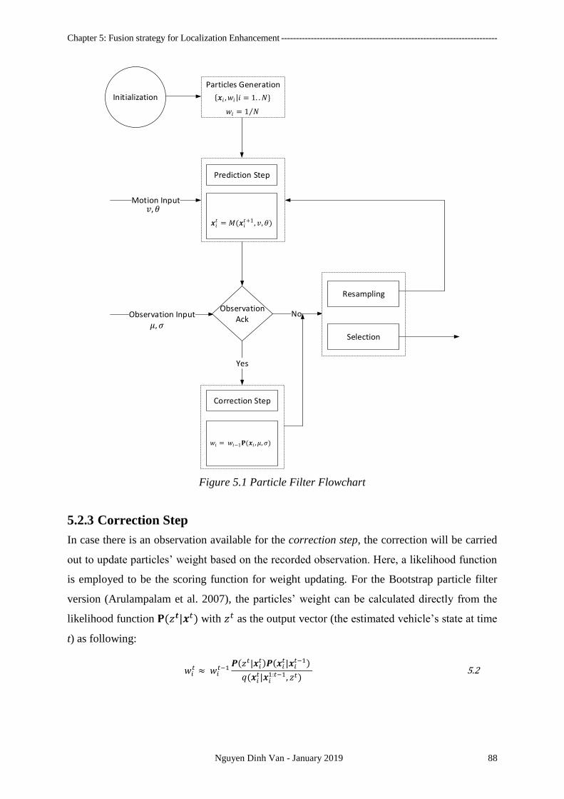
Chapter 5: Fusion strategy for Localization Enhancement -------------------------------------------------------------------------
Nguyen Dinh Van - January 2019 88
Initialization
Particles Generation
Motion Input
Observation Input
Yes
No
Resampling
Selection
Prediction Step
Observation Ack
Correction Step
𝑣, 𝜃
𝜇,𝜎
𝒙𝑖𝑡 = 𝑀(𝒙𝑖
𝑡+1 ,𝑣,𝜃)
𝒙𝑖 ,𝑤𝑖|𝑖 = 1. .𝑁
𝑤𝑖 = 1 𝑁
𝑤𝑖 = 𝑤𝑖−1𝚸(𝒙𝑖 ,𝜇,𝜎)
Figure 5.1 Particle Filter Flowchart
5.2.3 Correction Step
In case there is an observation available for the correction step, the correction will be carried
out to update particles’ weight based on the recorded observation. Here, a likelihood function
is employed to be the scoring function for weight updating. For the Bootstrap particle filter
version (Arulampalam et al. 2007), the particles’ weight can be calculated directly from the
likelihood function 𝚸(𝑧𝒕|𝒙𝑡) with 𝑧𝑡 as the output vector (the estimated vehicle’s state at time
t) as following:
𝑤𝑖𝑡 ≈ 𝑤𝑖
𝑡−1𝜬(𝑧𝑡|𝒙𝑖
𝑡)𝜬(𝒙𝑖𝑡|𝒙𝑖
𝑡−1)
𝑞(𝒙𝑖𝑡|𝒙𝑖
1:𝑡−1, 𝑧𝑡) 5.2
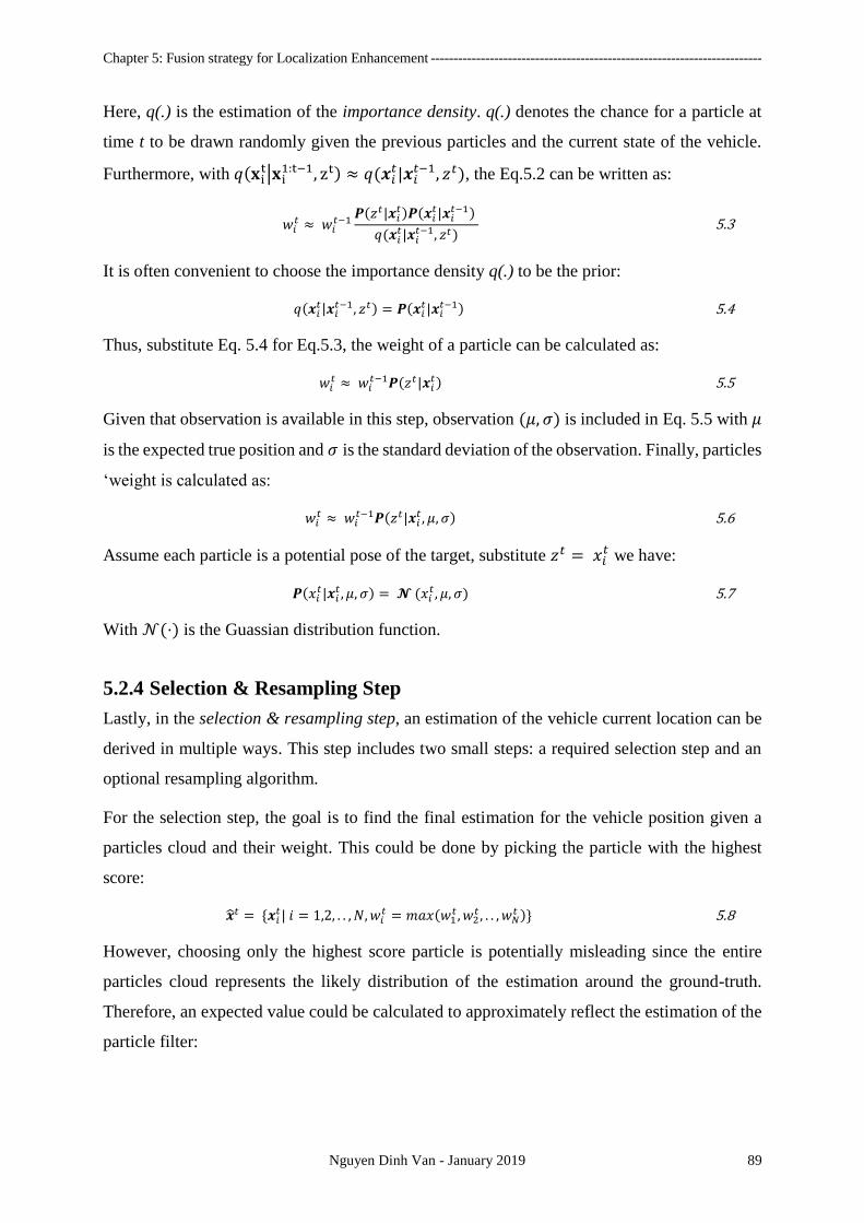
Chapter 5: Fusion strategy for Localization Enhancement -------------------------------------------------------------------------
Nguyen Dinh Van - January 2019 89
Here, q(.) is the estimation of the importance density. q(.) denotes the chance for a particle at
time t to be drawn randomly given the previous particles and the current state of the vehicle.
Furthermore, with 𝑞(𝐱it|𝐱i
1:t−1, zt) ≈ 𝑞(𝒙𝑖𝑡|𝒙𝑖
𝑡−1, 𝑧𝑡), the Eq.5.2 can be written as:
𝑤𝑖𝑡 ≈ 𝑤𝑖
𝑡−1𝜬(𝑧𝑡|𝒙𝑖
𝑡)𝜬(𝒙𝑖𝑡|𝒙𝑖
𝑡−1)
𝑞(𝒙𝑖𝑡|𝒙𝑖
𝑡−1, 𝑧𝑡) 5.3
It is often convenient to choose the importance density q(.) to be the prior:
𝑞(𝒙𝑖𝑡|𝒙𝑖
𝑡−1, 𝑧𝑡) = 𝜬(𝒙𝑖𝑡|𝒙𝑖
𝑡−1) 5.4
Thus, substitute Eq. 5.4 for Eq.5.3, the weight of a particle can be calculated as:
𝑤𝑖𝑡 ≈ 𝑤𝑖
𝑡−1𝜬(𝑧𝑡|𝒙𝑖𝑡) 5.5
Given that observation is available in this step, observation (𝜇, 𝜎) is included in Eq. 5.5 with 𝜇
is the expected true position and 𝜎 is the standard deviation of the observation. Finally, particles
‘weight is calculated as:
𝑤𝑖𝑡 ≈ 𝑤𝑖
𝑡−1𝜬(𝑧𝑡|𝒙𝑖𝑡 , 𝜇, 𝜎) 5.6
Assume each particle is a potential pose of the target, substitute 𝑧𝑡 = 𝑥𝑖𝑡 we have:
𝜬(𝑥𝑖𝑡|𝒙𝑖
𝑡 , 𝜇, 𝜎) = 𝓝 (𝑥𝑖𝑡 , 𝜇, 𝜎) 5.7
With 𝒩(⋅) is the Guassian distribution function.
5.2.4 Selection & Resampling Step
Lastly, in the selection & resampling step, an estimation of the vehicle current location can be
derived in multiple ways. This step includes two small steps: a required selection step and an
optional resampling algorithm.
For the selection step, the goal is to find the final estimation for the vehicle position given a
particles cloud and their weight. This could be done by picking the particle with the highest
score:
𝒙𝑡 = 𝒙𝑖𝑡| 𝑖 = 1,2, . . , 𝑁, 𝑤𝑖
𝑡 = 𝑚𝑎𝑥(𝑤1𝑡 , 𝑤2
𝑡 , . . , 𝑤𝑁𝑡 ) 5.8
However, choosing only the highest score particle is potentially misleading since the entire
particles cloud represents the likely distribution of the estimation around the ground-truth.
Therefore, an expected value could be calculated to approximately reflect the estimation of the
particle filter:
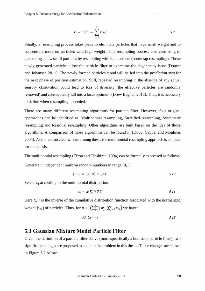
Chapter 5: Fusion strategy for Localization Enhancement -------------------------------------------------------------------------
Nguyen Dinh Van - January 2019 90
𝒙𝑡 = 𝐸[𝒙𝑡] = ∑𝒙𝑖𝑡𝑤𝑖
𝑡
𝑁
𝑖=1
5.9
Finally, a resampling process takes place to eliminate particles that have small weight and to
concentrate more on particles with high weight. This resampling process also consisting of
generating a new set of particles by resampling with replacement (bootstrap resampling). Those
newly generated particles allow the particle filter to overcome the degeneracy issue (Doucet
and Johansen 2011). The newly formed particles cloud will be fed into the prediction step for
the next phase of position estimation. Still, repeated resampling in the absence of any actual
sensory observation could lead to loss of diversity (the effective particles are randomly
removed) and consequently fall into a local optimum (Drew Bagnell 2018). Thus, it is necessary
to define when resampling is needed.
There are many different resampling algorithms for particle filter. However, four original
approaches can be identified as: Multinomial resampling, Stratified resampling, Systematic
resampling and Residual resampling. Other algorithms are built based on the idea of those
algorithms. A comparison of those algorithms can be found in (Douc, Cappé, and Moulines
2005). As there is no clear winner among these, the multinomial resampling approach is adopted
for this thesis.
The multinomial resampling (Efron and Tibshirani 1994) can be formally expressed as follows:
Generate n independent uniform random numbers in range (0,1]:
𝑈𝑖 |𝑖 = 1,2. . 𝑛 ∈ (0,1] 5.10
Select 𝒙𝑖 according to the multinomial distribution:
𝒙𝑖 = 𝒙(𝐹𝑤−1(𝑈𝑖)) 5.11
Here 𝐹𝑤−1 is the inverse of the cumulative distribution function associated with the normalized
weight 𝑤𝑖 of particles. Thus, for 𝑢 ∈ (∑ 𝑤𝑗𝑖−1𝑗=1 , ∑ 𝑤𝑗
𝑖𝑗=1 ) we have:
𝐹𝑤−1(𝑢) = 𝑖 5.12
5.3 Gaussian Mixture Model Particle Filter
Given the definition of a particle filter above (more specifically a bootstrap particle filter), two
significant changes are proposed to adapt to the problem in this thesis. Those changes are shown
in Figure 5.2 below.
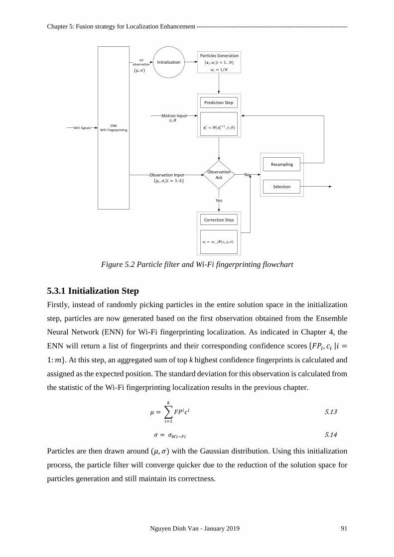
Chapter 5: Fusion strategy for Localization Enhancement -------------------------------------------------------------------------
Nguyen Dinh Van - January 2019 91
Initialization
Particles Generation
Motion Input
Yes
No
Resampling
Selection
Prediction Step
Observation Ack
Correction Step
𝑣, 𝜃
𝜇𝑖 ,𝜎𝑖|𝑖 = 1: 𝑘
𝒙𝑖𝑡 = 𝑀(𝒙𝑖
𝑡+1 ,𝑣,𝜃)
𝒙𝑖 ,𝑤𝑖|𝑖 = 1. .𝑁
𝑤𝑖 = 1 𝑁
𝑤𝑖 = 𝑤𝑖−1𝚸(𝑥𝑖 ,𝜇,𝜎)
ENNWiFi Fingerprinting
1st observation
WiFi Signals
(𝜇,𝜎)
Figure 5.2 Particle filter and Wi-Fi fingerprinting flowchart
5.3.1 Initialization Step
Firstly, instead of randomly picking particles in the entire solution space in the initialization
step, particles are now generated based on the first observation obtained from the Ensemble
Neural Network (ENN) for Wi-Fi fingerprinting localization. As indicated in Chapter 4, the
ENN will return a list of fingerprints and their corresponding confidence scores 𝐹𝑃𝑖, 𝑐𝑖 |𝑖 =
1:𝑚. At this step, an aggregated sum of top k highest confidence fingerprints is calculated and
assigned as the expected position. The standard deviation for this observation is calculated from
the statistic of the Wi-Fi fingerprinting localization results in the previous chapter.
𝜇 = ∑𝐹𝑃𝑖𝑐𝑖𝑘
𝑖=1
5.13
𝜎 = 𝜎𝑊𝑖−𝐹𝑖 5.14
Particles are then drawn around (𝜇, 𝜎) with the Gaussian distribution. Using this initialization
process, the particle filter will converge quicker due to the reduction of the solution space for
particles generation and still maintain its correctness.
Chapter 5: Fusion strategy for Localization Enhancement -------------------------------------------------------------------------
Nguyen Dinh Van - January 2019 92
5.3.2 Correction Step
Secondly, a Gaussian mixture model is applied for the observation in the correction step.
Similar to the initialization step, a top k highest confidence fingerprints will be taken into
account for the correction. Eq.5.6 is then written as follows:
𝑤𝑡𝑖 = 𝑤𝑡−1
𝑖 ∑𝑐𝑗
∑ 𝑐𝑗𝑘𝑗=1
𝜬(𝒙𝑡𝑖 |𝜎𝑡
𝑗, 𝜇𝑡
𝑗)
𝑘
𝑗=1
5.15
Here, 𝜇𝑡𝑗 is the 𝑗𝑡ℎ highest confidence fingerprint 𝐹𝑃𝑗 and 𝜎𝑡
𝑗 is related to the measured
standard deviation of the Wi-Fi fingerprint as follows:
𝜎𝑡𝑗= 1 −
𝑐𝑗
∑ 𝑐𝑗𝑘𝑗=1
𝜎𝑊𝑖−𝐹𝑖 5.16
The underlying assumption in Eq.5.16 is as the confidence of the fingerprint becomes lower,
its standard deviation should increase.
Assume that the mixture distribution follows a Gaussian distribution then Eq. 5.15 is:
𝑤𝑡𝑖 = 𝑤𝑡−1
𝑖 ∑𝑐𝑗
∑ 𝑐𝑗𝑘𝑗=1
𝑘
𝑗=1
1
√2𝜋(𝜎𝑡𝑗)2
𝑒−(𝒙𝑡
𝑖−𝜇𝑡𝑗)2
⁄(𝜎𝑡
𝑗)2 5.17
The Gaussian mixture model is utilized to enhance the weighting function. Consider a case
where three top fingerprints are chosen (k = 3). The normalized confidence scores for these
fingerprints are 0.58, 0.277 and 0.143 respectively. An illustration of particle weight is shown
in Figure 5.3. In this example, a 20m by 20m area is taken into account with each particle drawn
in every 10cm cell with the same weight. Using the Gaussian mixture model scoring function
in Eq.5.17, each particle’s weight is calculated regarding the confidence score of each
fingerprint. The final estimation is an aggregated sum of all particles with their weight as in
Eq.5.18.
𝒙𝑡 = ∑𝒙𝑖𝑡𝑤𝑖
𝑡
𝑁
𝑖=1
5.18
Unlike a single Gaussian model estimation approach where only the highest confidence
fingerprint is chosen (k =1), the approach with Gaussian mixture model estimation allows the
final estimation to be closer to the true position. This happens due to in single Gaussian
estimation, if particles are generated uniformly over the entire solution space, then the final
estimation should be at exactly the highest confidence fingerprint as in Figure 5.4. Thus, the
Gaussian mixture model should deliver better estimation for particles’ weight.

Chapter 5: Fusion strategy for Localization Enhancement -------------------------------------------------------------------------
Nguyen Dinh Van - January 2019 93
Figure 5.3 Gaussian Mixture Model Estimation
Figure 5.4 Single Gaussian Model Estimation
A real case scenario of the Gaussian Mixture Model in practice can be seen in Figure 5.5 and
Figure 5.6. In the two figures, the fingerprints of the environment are shown in blues. The
ground-truth and the estimated position are shown in green and yellow respectively. With three
top highest confidence fingerprints are chosen for the Gaussian mixture model (k = 3), each of
these fingerprints’ confidence score is proportional to the red circle’s size.
In Figure 5.5, the highest confidence fingerprint is also a good classification from the Ensemble
Neural Networks (the closest to the ground-truth in terms of Euclidian distance – Section 4.4.2).
The final estimation is carried out based on two factors: The propagated particles cloud from
the previous step using the motion model and re-evaluation of the particles ‘weights with new
observations. With a good classification from the Ensemble Neural Networks, particles that are
closer to the highest confidence fingerprint should also have higher weights. Suppose that the
propagated particles cloud correctly covers the vehicle’s true position (in the ideal case, the true
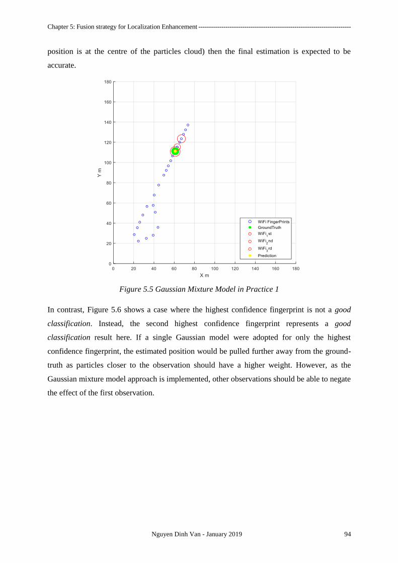
Chapter 5: Fusion strategy for Localization Enhancement -------------------------------------------------------------------------
Nguyen Dinh Van - January 2019 94
position is at the centre of the particles cloud) then the final estimation is expected to be
accurate.
Figure 5.5 Gaussian Mixture Model in Practice 1
In contrast, Figure 5.6 shows a case where the highest confidence fingerprint is not a good
classification. Instead, the second highest confidence fingerprint represents a good
classification result here. If a single Gaussian model were adopted for only the highest
confidence fingerprint, the estimated position would be pulled further away from the ground-
truth as particles closer to the observation should have a higher weight. However, as the
Gaussian mixture model approach is implemented, other observations should be able to negate
the effect of the first observation.
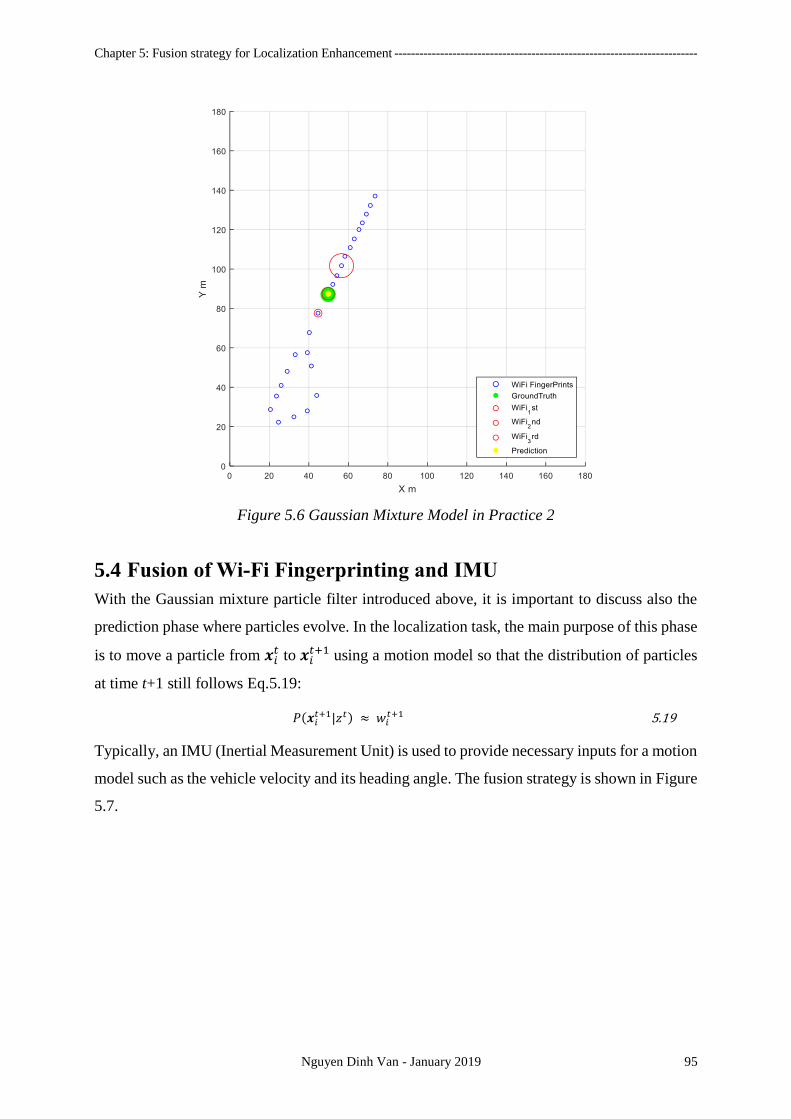
Chapter 5: Fusion strategy for Localization Enhancement -------------------------------------------------------------------------
Nguyen Dinh Van - January 2019 95
Figure 5.6 Gaussian Mixture Model in Practice 2
5.4 Fusion of Wi-Fi Fingerprinting and IMU
With the Gaussian mixture particle filter introduced above, it is important to discuss also the
prediction phase where particles evolve. In the localization task, the main purpose of this phase
is to move a particle from 𝒙𝑖𝑡 to 𝒙𝑖
𝑡+1 using a motion model so that the distribution of particles
at time t+1 still follows Eq.5.19:
𝛲(𝒙𝑖𝑡+1|𝑧𝑡) ≈ 𝑤𝑖
𝑡+1 5.19
Typically, an IMU (Inertial Measurement Unit) is used to provide necessary inputs for a motion
model such as the vehicle velocity and its heading angle. The fusion strategy is shown in Figure
5.7.
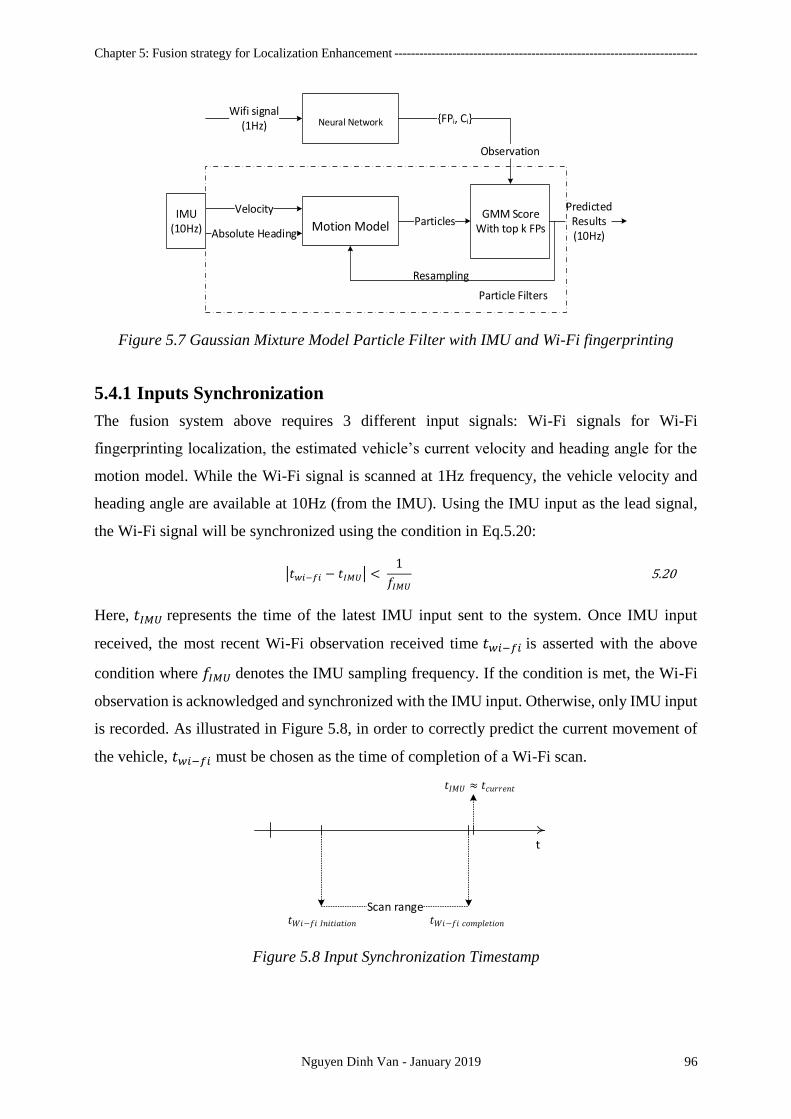
Chapter 5: Fusion strategy for Localization Enhancement -------------------------------------------------------------------------
Nguyen Dinh Van - January 2019 96
Neural NetworkWifi signal
(1Hz)FPi, Ci
Motion Model
Velocity
Absolute HeadingParticles
GMM ScoreWith top k FPs
Predicted Results(10Hz)
Observation
Particle Filters
Resampling
IMU(10Hz)
Figure 5.7 Gaussian Mixture Model Particle Filter with IMU and Wi-Fi fingerprinting
5.4.1 Inputs Synchronization
The fusion system above requires 3 different input signals: Wi-Fi signals for Wi-Fi
fingerprinting localization, the estimated vehicle’s current velocity and heading angle for the
motion model. While the Wi-Fi signal is scanned at 1Hz frequency, the vehicle velocity and
heading angle are available at 10Hz (from the IMU). Using the IMU input as the lead signal,
the Wi-Fi signal will be synchronized using the condition in Eq.5.20:
|𝑡𝑤𝑖−𝑓𝑖 − 𝑡𝐼𝑀𝑈| < 1
𝑓𝐼𝑀𝑈
5.20
Here, 𝑡𝐼𝑀𝑈 represents the time of the latest IMU input sent to the system. Once IMU input
received, the most recent Wi-Fi observation received time 𝑡𝑤𝑖−𝑓𝑖 is asserted with the above
condition where 𝑓𝐼𝑀𝑈 denotes the IMU sampling frequency. If the condition is met, the Wi-Fi
observation is acknowledged and synchronized with the IMU input. Otherwise, only IMU input
is recorded. As illustrated in Figure 5.8, in order to correctly predict the current movement of
the vehicle, 𝑡𝑤𝑖−𝑓𝑖 must be chosen as the time of completion of a Wi-Fi scan.
t
Scan range𝑡𝑊𝑖−𝑓𝑖 𝐼𝑛𝑖𝑡𝑖𝑎𝑡𝑖𝑜𝑛 𝑡𝑊𝑖−𝑓𝑖 𝑐𝑜𝑚𝑝𝑙𝑒𝑡𝑖𝑜𝑛
𝑡𝐼𝑀𝑈 ≈ 𝑡𝑐𝑢𝑟𝑟𝑒𝑛𝑡
Figure 5.8 Input Synchronization Timestamp
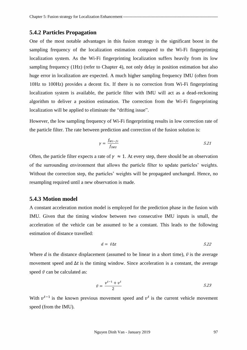
Chapter 5: Fusion strategy for Localization Enhancement -------------------------------------------------------------------------
Nguyen Dinh Van - January 2019 97
5.4.2 Particles Propagation
One of the most notable advantages in this fusion strategy is the significant boost in the
sampling frequency of the localization estimation compared to the Wi-Fi fingerprinting
localization system. As the Wi-Fi fingerprinting localization suffers heavily from its low
sampling frequency (1Hz) (refer to Chapter 4), not only delay in position estimation but also
huge error in localization are expected. A much higher sampling frequency IMU (often from
10Hz to 100Hz) provides a decent fix. If there is no correction from Wi-Fi fingerprinting
localization system is available, the particle filter with IMU will act as a dead-reckoning
algorithm to deliver a position estimation. The correction from the Wi-Fi fingerprinting
localization will be applied to eliminate the “drifting issue”.
However, the low sampling frequency of Wi-Fi fingerprinting results in low correction rate of
the particle filter. The rate between prediction and correction of the fusion solution is:
𝛾 = 𝑓𝑊𝑖−𝑓𝑖
𝑓𝐼𝑀𝑈
5.21
Often, the particle filter expects a rate of 𝛾 ≈ 1. At every step, there should be an observation
of the surrounding environment that allows the particle filter to update particles’ weights.
Without the correction step, the particles’ weights will be propagated unchanged. Hence, no
resampling required until a new observation is made.
5.4.3 Motion model
A constant acceleration motion model is employed for the prediction phase in the fusion with
IMU. Given that the timing window between two consecutive IMU inputs is small, the
acceleration of the vehicle can be assumed to be a constant. This leads to the following
estimation of distance travelled:
𝑑 = ∆𝑡 5.22
Where 𝑑 is the distance displacement (assumed to be linear in a short time), is the average
movement speed and ∆𝑡 is the timing window. Since acceleration is a constant, the average
speed can be calculated as:
= 𝑣𝑡−1 + 𝑣𝑡
2 5.23
With 𝑣𝑡−1 is the known previous movement speed and 𝑣𝑡 is the current vehicle movement
speed (from the IMU).
Chapter 5: Fusion strategy for Localization Enhancement -------------------------------------------------------------------------
Nguyen Dinh Van - January 2019 98
For each particle 𝒙𝑖𝑡(𝑥𝑖
𝑡, 𝑦𝑖𝑡), with the absolute heading angle 𝜃 and the displacement distance d
the coordinate is calculated as:
𝑥𝑖𝑡 = 𝑥𝑖
𝑡−1 + ∆𝑡𝑐𝑜𝑠(𝜃) 5.24
And:
𝑦𝑖𝑡 = 𝑦𝑖
𝑡−1 + ∆𝑡𝑠𝑖𝑛(𝜃) 5.25
However, the unbiased Gaussian noise of IMU measurement should be included as in:
(
) ~ 𝒩((
𝑣
𝜃) , (
𝜎𝑣 0
0 𝜎𝜃)) 5.26
Thus, Eq.5.24 and Eq.5.25 can be rewritten as:
(𝑥 𝑖𝑡
𝑦 𝑖𝑡) = (
𝑥𝑖𝑡−1 +
𝑡−1 + 𝑡
2∆𝑡 𝑐𝑜𝑠 ()
𝑦𝑖𝑡−1 +
𝑡−1 + 𝑡
2∆𝑡 𝑠𝑖𝑛 ()
) 5.27
This demonstrates that for each particle 𝒙𝑖𝑡−1, a newly predicted particle 𝒙𝑖
𝑡 is drawn using the
IMU inputs , with their respective Gaussian distribution 𝒩(𝑣, 𝜎𝑣), 𝒩(𝜃, 𝜎𝜃). The resulting
particle cloud therefore closely follow the prior density 𝑝(𝑧𝑡|𝑧𝑡−1, , ).
5.4.4 Selection & Resampling
Regarding the IMU fusion solution, the resampling step is skipped when there is no new
observation recorded. Without new observation, resampling the particles will likely to introduce
diversity loss problem. Moreover, when there is a new observation, the resampling step is only
required when the number of ineffective particles (particles with their weight approaching zero)
is large. A large number of approximately zero weight particles would contribute to a significant
part to the approximation of the assumed distribution and therefore distorts the result. In order
to determine when the resampling is needed, we define a Coefficient of Variation (CV) as
follows:
𝐶𝑉 = 𝑉𝐴𝑅(𝑤𝑖)
𝐸2[𝑤𝑖] 5.28
With
𝑉𝐴𝑅(𝑤𝑖) = 1
𝑁∑(𝑤𝑖 −
1
𝑁∑𝑤𝑖
𝑁
𝑖=1
)
2𝑁
𝑖=1
5.29
And

Chapter 5: Fusion strategy for Localization Enhancement -------------------------------------------------------------------------
Nguyen Dinh Van - January 2019 99
𝐸2[𝑤𝑖] = (1
𝑁∑𝑤𝑖
𝑁
𝑖=1
)2 5.30
Hence, the CV can be written as:
𝐶𝑉 = 1
𝑁∑(𝑁 ∙ 𝑤𝑖 − 1)2𝑁
𝑖=1
5.31
Using this coefficient, the Effective Particle Size (EPS) can then be calculated as
𝐸𝑃𝑆 = 𝑁
1 + 𝐶𝑉 5.32
This number describes how many particles that have an effective weight (not approximately
zero). If more than half of the particles are effective, the resampling process is not required.
𝐸𝑃𝑆 <1
2𝑁 5.33
5.5 Fusion of Wi-Fi Fingerprinting, IMU and Laser-SLAM
For intelligent vehicles, one of the most commonly elaborated localization fusion systems is a
fusion of GPS and laser-based SLAM. The concept of localization using laser-based SLAM,
which is discussed in Section 2.3, has two key steps: building the map of the environment using
laser scans while simultaneously determining the relative position of the vehicle to the newly
built map. Coupling this method with GPS signals brings not only the possibility of translating
local localization results to global ones but also allows to provide an absolute correction for the
drifting issue of SLAM (Bresson et al. 2016; Boucher, Ababsa, and Mallem 2013). Fusion
solutions for SLAM and GPS can be found in (Kim 2004; Carlson, Thorpe, and Browning 2010;
Pierzchała, Giguère, and Astrup 2018; Levinson, Montemerlo, and Thrun 2008; Trehard et al.
2014). Thus it is interesting to discuss a potential integration of the IMU, the Wi-Fi
fingerprinting system with a laser-SLAM which: (1) Enables the GPS-denied environment
global localization and mapping (2) Allows smooth transition between GPS-denied
environment to GPS-aided one and (3) Enhances localization results. In general, there are two
ways to fuse the laser-SLAM with an absolute localization system: (1) translate SLAM into
global coordinate frame approach and (2) SLAM as a highly accurate pseudo-IMU.
In the first approach, the SLAM local coordinate system needs to be translated into a global
coordinate frame. To do so, there is a need for a proper translation and rotation matrix between
the local coordinate system of SLAM and the global coordinate system. This could be done by
Chapter 5: Fusion strategy for Localization Enhancement -------------------------------------------------------------------------
Nguyen Dinh Van - January 2019 100
using an algorithm such as Iterative Closest Points (ICP) (Besl and McKay 1992).
Unfortunately, the ICP algorithm requires a proper initial value and the approximate registration
of two laser point clouds to prevent the algorithm from failing into local optima (Y. He et al.
2017; Agamennoni et al. 2016). These conditions are difficult to achieve in the real life
situation. Another way to establish the transformation matrix is to use the absolute static map
of the environment as a reference. However, any bias in the static map will also be included in
the transformation matrix as well. Furthermore, obtaining a highly accurate static map of the
environment such as a carpark is a costly task as well.
An alternative approach for fusing laser-SLAM with an absolute localization system is to use
laser-SLAM as a highly accurate IMU. Since laser-SLAM returns local estimation of distance
displacement as well as heading changes with the accuracy up to centimetres, it is possible to
calculate the temporal velocity and yaw rate. This approach, however, cannot fully exploit the
benefit of the detailed environment map created by laser sensors in the SLAM algorithm.
In this thesis, both approaches for fusing laser-SLAM with the Wi-Fi fingerprinting localization
system are examined. Since we want to eliminate the complex initialization as well as map
building process of the environment using SLAM, the thesis will only deal with first time
SLAM case. This means the vehicle is assumed to have no prior laser map of the environment
nor a complex ICP calibration for the starting point. Thus, it is expected that most SLAM
solutions will suffer from the drifting issue.
One part of this thesis work is to investigate the possible fusion of Wi-Fi localization and laser-
based SLAM. To the best of the author’s knowledge, there is no current attempt to fusion those
two interesting methods together. Two representative approaches for laser-based SLAM are
chosen for further analysis: the evidential-based C-SLAM (Trehard et al. 2014) and the
probabilistic-based PML-SLAM (Alsayed et al. 2015). A quick review of the two SLAM
algorithms will be presented in this section.
5.5.1 Evidential SLAM
From the beginning, a probabilistic background is chosen for the Simultaneous Localization
and Mapping (SLAM) problem. However, a new approach using the evidential theory is studied
in an attempt to overcome the limitation of the classical one. The main argument is for the
online-SLAM (or other Maximum-Likelihood SLAMs), only the maximum position is searched
and propagated to the next time step. In addition, the constructed map is built with respect to
the maxima. Hence, all uncertainties related to the vehicle pose and map states are simply
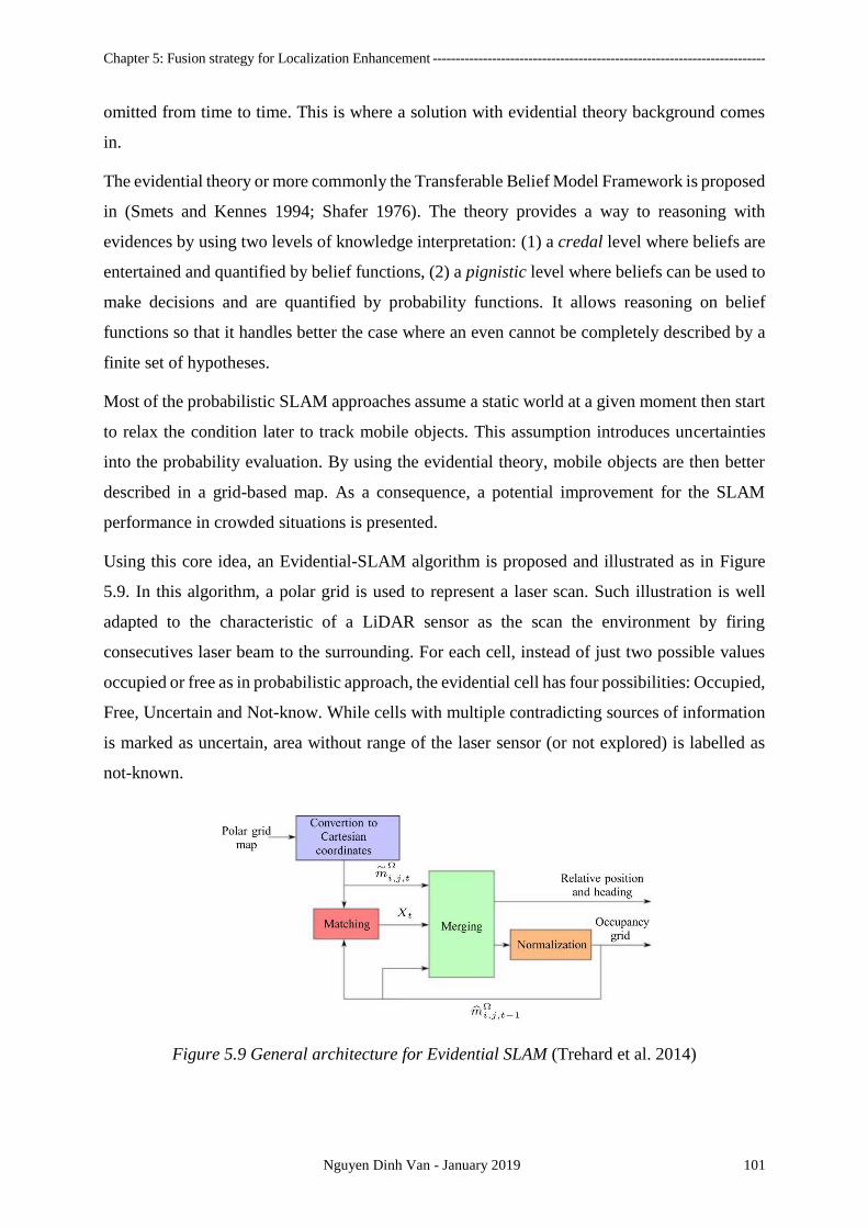
Chapter 5: Fusion strategy for Localization Enhancement -------------------------------------------------------------------------
Nguyen Dinh Van - January 2019 101
omitted from time to time. This is where a solution with evidential theory background comes
in.
The evidential theory or more commonly the Transferable Belief Model Framework is proposed
in (Smets and Kennes 1994; Shafer 1976). The theory provides a way to reasoning with
evidences by using two levels of knowledge interpretation: (1) a credal level where beliefs are
entertained and quantified by belief functions, (2) a pignistic level where beliefs can be used to
make decisions and are quantified by probability functions. It allows reasoning on belief
functions so that it handles better the case where an even cannot be completely described by a
finite set of hypotheses.
Most of the probabilistic SLAM approaches assume a static world at a given moment then start
to relax the condition later to track mobile objects. This assumption introduces uncertainties
into the probability evaluation. By using the evidential theory, mobile objects are then better
described in a grid-based map. As a consequence, a potential improvement for the SLAM
performance in crowded situations is presented.
Using this core idea, an Evidential-SLAM algorithm is proposed and illustrated as in Figure
5.9. In this algorithm, a polar grid is used to represent a laser scan. Such illustration is well
adapted to the characteristic of a LiDAR sensor as the scan the environment by firing
consecutives laser beam to the surrounding. For each cell, instead of just two possible values
occupied or free as in probabilistic approach, the evidential cell has four possibilities: Occupied,
Free, Uncertain and Not-know. While cells with multiple contradicting sources of information
is marked as uncertain, area without range of the laser sensor (or not explored) is labelled as
not-known.
Figure 5.9 General architecture for Evidential SLAM (Trehard et al. 2014)

Chapter 5: Fusion strategy for Localization Enhancement -------------------------------------------------------------------------
Nguyen Dinh Van - January 2019 102
Each cell in the map is evaluated using Evidence Theory will have a basic belief assignment of
following set:
2𝛺 = 𝐹𝑟𝑒𝑒, 𝑂𝑐𝑐𝑢𝑝𝑖𝑒𝑑, 𝛺, ∅ 5.34
Where
∑ 𝑚Ω (𝑥) = 1
𝑥 ∈ 2Ω
5.35
With m is defined as a mass (or a weight) of a hypothesis and x is all four possible cases.
A map is then estimated by comparing the information with the previous known map through
the map matching process. Information will be merged (newly obtained map and old map) and
the relative position of the vehicle is calculated.
Evaluation on the KITTI database shows a 1.3% of translation error and 6.2 degree of rotational
error after a 2.2km test drive. Test drive and the localization result is shown in Figure 5.10.
Figure 5.10 Evidential SLAM test drive in KITTI database (Trehard et al. 2014)
5.5.2 PML-SLAM
The PML-SLAM (stands for Probabilistic Maximum Likelihood SLAM) is a version of SLAM
that belongs to the classical probabilistic background category. In contrast to the Evidential
SLAM presented in section 5.5.1, the study in (Alsayed et al. 2015) proposes a complete
solution with large scale map management, maximum likelihood scoring function and an
adaptive parameter matching algorithm. The general architecture is presented in Figure 5.11.

Chapter 5: Fusion strategy for Localization Enhancement -------------------------------------------------------------------------
Nguyen Dinh Van - January 2019 103
Figure 5.11 General flowchart of the PML-SLAM algorithm (Alsayed et al. 2015)
Although the maximum likelihood matching and grid map of this solution are generally similar
to other probabilistic based SLAM approaches, the solution does propose a large scale
environment map management which is crucial for a real life application. The solution is then
validated on the KITTI database (Figure 5.12) with promising results of 5cm of displacement
error and 0.3 degree of heading error. After more than 2.2km of traveling, the accumulated error
in localization is about 6m with 0.1 degree of heading error. The deviation in distance and
heading are shown in Figure 5.13.
Figure 5.12 Test drive on KITTI database with PML-SLAM (Alsayed et al. 2015)
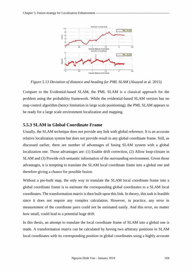
Chapter 5: Fusion strategy for Localization Enhancement -------------------------------------------------------------------------
Nguyen Dinh Van - January 2019 104
Figure 5.13 Deviation of distance and heading for PML SLAM (Alsayed et al. 2015)
Compare to the Evidential-based SLAM, the PML SLAM is a classical approach for the
problem using the probability framework. While the evidential-based SLAM version has no
map control algorithm (hence limitation in large scale positioning), the PML SLAM appears to
be ready for a large scale environment localization and mapping.
5.5.3 SLAM in Global Coordinate Frame
Usually, the SLAM technique does not provide any link with global reference. It is an accurate
relative localization system but does not provide result in any global coordinate frame. Still, as
discussed earlier, there are number of advantages of fusing SLAM system with a global
localization one. Those advantages are: (1) Enable drift correction, (2) Allow loop-closure in
SLAM and (3) Provide rich semantic information of the surrounding environment. Given those
advantages, it is tempting to translate the SLAM local coordinate frame into a global one and
therefore giving a chance for possible fusion.
Without a pre-built map, the only way to translate the SLAM local coordinate frame into a
global coordinate frame is to estimate the corresponding global coordinates to a SLAM local
coordinates. The transformation matrix is then built upon this link. In theory, this task is feasible
since it does not require any complex calculation. However, in practice, any error in
measurement of the coordinate pairs could not be estimated easily. And this error, no matter
how small, could lead to a potential huge drift.
In this thesis, an attempt to translate the local coordinate frame of SLAM into a global one is
made. A transformation matrix can be calculated by having two arbitrary positions in SLAM
local coordinates with its corresponding position in global coordinates using a highly accurate
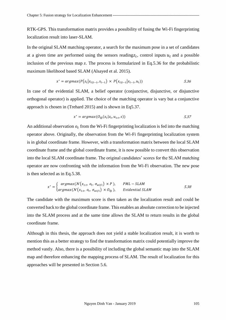
Chapter 5: Fusion strategy for Localization Enhancement -------------------------------------------------------------------------
Nguyen Dinh Van - January 2019 105
RTK-GPS. This transformation matrix provides a possibility of fusing the Wi-Fi fingerprinting
localization result into laser-SLAM.
In the original SLAM matching operator, a search for the maximum pose in a set of candidates
at a given time are performed using the sensors reading𝑧𝑡 , control inputs 𝑢𝑡 and a possible
inclusion of the previous map 𝑠. The process is formularized in Eq.5.36 for the probabilistic
maximum likelihood based SLAM (Alsayed et al. 2015).
𝑥∗ = 𝑎𝑟𝑔𝑚𝑎𝑥(𝑃(𝑧𝑡|𝑥𝑡|𝑡−1, 𝑠𝑡−1) × 𝑃(𝑥𝑡|𝑡−1|𝑥𝑡−1, 𝑢𝑡)) 5.36
In case of the evidential SLAM, a belief operator (conjunctive, disjunctive, or disjunctive
orthogonal operator) is applied. The choice of the matching operator is vary but a conjunctive
approach is chosen in (Trehard 2015) and is shown in Eq5.37.
𝑥∗ = 𝑎𝑟𝑔𝑚𝑎𝑥(𝒪⊕(𝑥𝑡|𝑧𝑡 , 𝑢1:𝑡 , 𝑠)) 5.37
An additional observation 𝑜𝑡 from the Wi-Fi fingerprinting localization is fed into the matching
operator above. Originally, the observation from the Wi-Fi fingerprinting localization system
is in global coordinate frame. However, with a transformation matrix between the local SLAM
coordinate frame and the global coordinate frame, it is now possible to convert this observation
into the local SLAM coordinate frame. The original candidates’ scores for the SLAM matching
operator are now confronting with the information from the Wi-Fi observation. The new pose
is then selected as in Eq.5.38.
𝑥∗ = 𝑎𝑟𝑔𝑚𝑎𝑥(𝒩(𝑥1:𝑡 , 𝑜𝑡 , 𝜎𝑤𝑖𝑓𝑖) × 𝑃 ), 𝑃𝑀𝐿 − 𝑆𝐿𝐴𝑀
𝑎𝑟𝑔𝑚𝑎𝑥(𝒩(𝑥1:𝑡 , 𝑜𝑡 , 𝜎𝑤𝑖𝑓𝑖) × 𝒪⊕ ), 𝐸𝑣𝑖𝑑𝑒𝑛𝑡𝑖𝑎𝑙 𝑆𝐿𝐴𝑀 5.38
The candidate with the maximum score is then taken as the localization result and could be
converted back to the global coordinate frame. This enables an absolute correction to be injected
into the SLAM process and at the same time allows the SLAM to return results in the global
coordinate frame.
Although in this thesis, the approach does not yield a stable localization result, it is worth to
mention this as a better strategy to find the transformation matrix could potentially improve the
method vastly. Also, there is a possibility of including the global semantic map into the SLAM
map and therefore enhancing the mapping process of SLAM. The result of localization for this
approaches will be presented in Section 5.6.
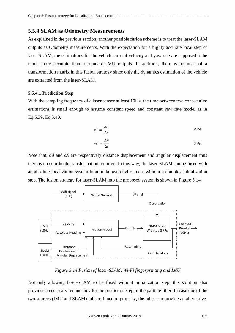
Chapter 5: Fusion strategy for Localization Enhancement -------------------------------------------------------------------------
Nguyen Dinh Van - January 2019 106
5.5.4 SLAM as Odometry Measurements
As explained in the previous section, another possible fusion scheme is to treat the laser-SLAM
outputs as Odometry measurements. With the expectation for a highly accurate local step of
laser-SLAM, the estimations for the vehicle current velocity and yaw rate are supposed to be
much more accurate than a standard IMU outputs. In addition, there is no need of a
transformation matrix in this fusion strategy since only the dynamics estimation of the vehicle
are extracted from the laser-SLAM.
5.5.4.1 Prediction Step
With the sampling frequency of a laser sensor at least 10Hz, the time between two consecutive
estimations is small enough to assume constant speed and constant yaw rate model as in
Eq.5.39, Eq.5.40.
𝑣𝑡 = ∆𝑑
∆𝑡 5.39
𝜔𝑡 = ∆𝜃
∆𝑡 5.40
Note that, ∆𝑑 and ∆𝜃 are respectively distance displacement and angular displacement thus
there is no coordinate transformation required. In this way, the laser-SLAM can be fused with
an absolute localization system in an unknown environment without a complex initialization
step. The fusion strategy for laser-SLAM into the proposed system is shown in Figure 5.14.
Neural NetworkWifi signal
(1Hz)FPi, Ci
Motion Model
Velocity
Absolute HeadingParticles
GMM ScoreWith top 3 FPs
Predicted Results(10Hz)
Particle Filters
Resampling
Observation
IMU(10Hz)
SLAM(10Hz) Angular Displacement
Distance Displacement
Figure 5.14 Fusion of laser-SLAM, Wi-Fi fingerprinting and IMU
Not only allowing laser-SLAM to be fused without initialization step, this solution also
provides a necessary redundancy for the prediction step of the particle filter. In case one of the
two sources (IMU and SLAM) fails to function properly, the other can provide an alternative.
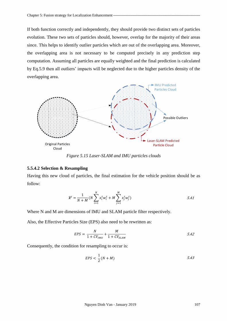
Chapter 5: Fusion strategy for Localization Enhancement -------------------------------------------------------------------------
Nguyen Dinh Van - January 2019 107
If both function correctly and independently, they should provide two distinct sets of particles
evolution. These two sets of particles should, however, overlap for the majority of their areas
since. This helps to identify outlier particles which are out of the overlapping area. Moreover,
the overlapping area is not necessary to be computed precisely in any prediction step
computation. Assuming all particles are equally weighted and the final prediction is calculated
by Eq.5.9 then all outliers’ impacts will be neglected due to the higher particles density of the
overlapping area.
Original Poi 0
Original Particles Cloud
Laser-SLAM Predicted Particle Cloud
IMU Predicted Particles Cloud
Possible Outliers
Figure 5.15 Laser-SLAM and IMU particles clouds
5.5.4.2 Selection & Resampling
Having this new cloud of particles, the final estimation for the vehicle position should be as
follow:
𝒙𝑡 =1
𝑁 +𝑀(𝑁∑𝑥𝑖
𝑡𝑤𝑖𝑡
𝑁
𝑖=1
+𝑀∑𝑥𝑗𝑡𝑤𝑗
𝑡
𝑀
𝑗=1
) 5.41
Where N and M are dimensions of IMU and SLAM particle filter respectively.
Also, the Effective Particles Size (EPS) also need to be rewritten as:
𝐸𝑃𝑆 = 𝑁
1 + 𝐶𝑉𝐼𝑀𝑈
+𝑀
1 + 𝐶𝑉𝑆𝐿𝐴𝑀 5.42
Consequently, the condition for resampling to occur is:
𝐸𝑃𝑆 < 1
2(𝑁 +𝑀) 5.43

Chapter 5: Fusion strategy for Localization Enhancement -------------------------------------------------------------------------
Nguyen Dinh Van - January 2019 108
5.6 Experiments and Results
5.6.1 Wi-Fi Fingerprinting Localization and IMU Fusion
In this section, experiments for the fusion system with IMU are presented. The experiments
setup are similar to the Wi-Fi fingerprinting localization experiments explained in Section 4.4.
Test runs will be conducted in INRIA campus, at Rocquencourt using two vehicles: a cybercar
and a Citroen C1 car.
Since the particle filter is a non-deterministic algorithm, several factors are examined such as:
number of particles required, the stability of the particle filter outcomes, particle filter
convergence given different starting conditions and results of the fusion solution under different
datasets.
Experiments of the Wi-Fi Fingerprinting and IMU fusion system will be explained with the
four steps of a particle filter: Initialization, Prediction, Correction and Selection & Resampling.
In each step, studies for some significant parameters and their impact to the particle filter will
be conducted and analysed in detail.
5.6.1.1 Initialization Step
The initialization phase has a significantly contribution to the convergence rate of the particle
filter. As there is no other prior knowledge assumed, the particle filter in this thesis will be
initialized with the first observation available from the Wi-Fi fingerprinting localization system.
In other word, at the first moment of entering the car park, the car will briefly wait for at most
one second for a positioning result from the Wi-Fi fingerprinting localization (since the
sampling frequency of the Wi-Fi system is 1Hz). Having the first classification results, the top
three fingerprints with highest confidence score will be selected. The weighted sum of these
fingerprints and their normalized scores will be calculated and taken as the assumed true
position as in Eq.5.44.
𝒙𝑡=0 = ∑𝐹𝑃𝑗𝑐𝑗
3
𝑗=1
5.44
With this first position, particles will be generated around it with 𝒙𝑡=0 as the expected mean
and the Wi-Fi standard deviation taken from statistic in experiments of Chapter 4 𝜎𝑤𝑖𝑓𝑖. Assume
the distribution of these particles follows Gaussian distribution, the 𝑖𝑡ℎ generated particle is
calculated as:
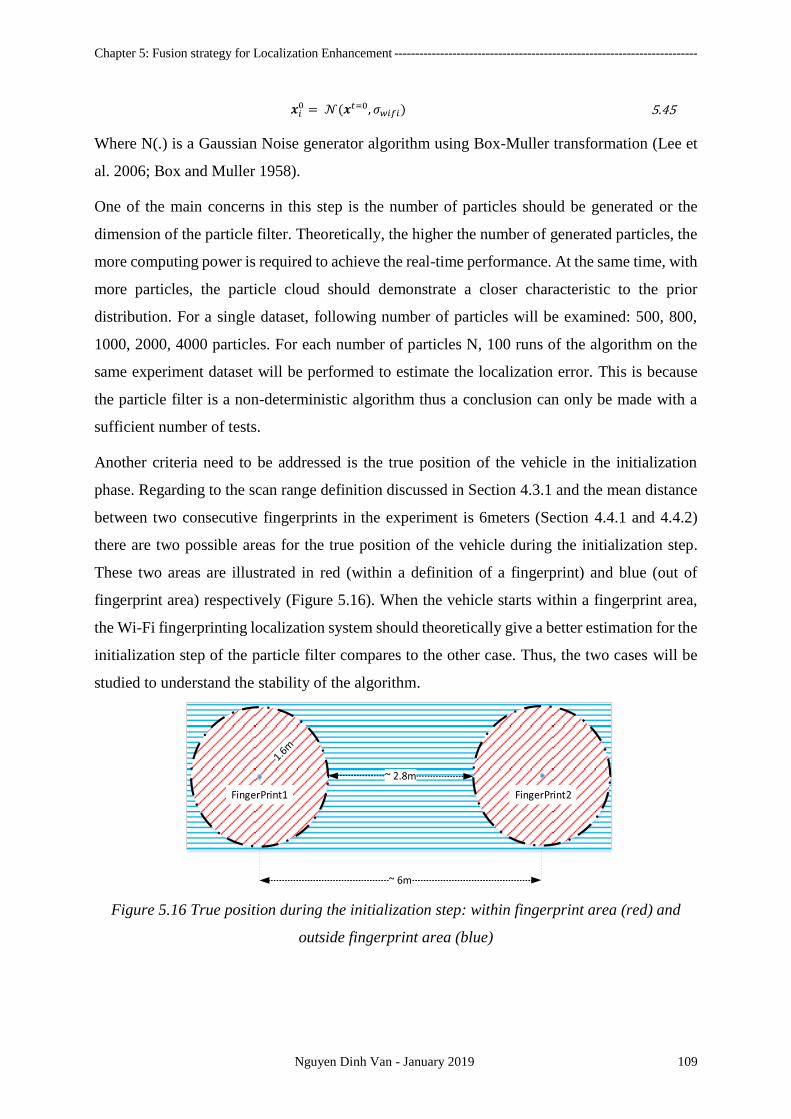
Chapter 5: Fusion strategy for Localization Enhancement -------------------------------------------------------------------------
Nguyen Dinh Van - January 2019 109
𝒙𝑖0 = 𝒩(𝒙𝑡=0, 𝜎𝑤𝑖𝑓𝑖) 5.45
Where N(.) is a Gaussian Noise generator algorithm using Box-Muller transformation (Lee et
al. 2006; Box and Muller 1958).
One of the main concerns in this step is the number of particles should be generated or the
dimension of the particle filter. Theoretically, the higher the number of generated particles, the
more computing power is required to achieve the real-time performance. At the same time, with
more particles, the particle cloud should demonstrate a closer characteristic to the prior
distribution. For a single dataset, following number of particles will be examined: 500, 800,
1000, 2000, 4000 particles. For each number of particles N, 100 runs of the algorithm on the
same experiment dataset will be performed to estimate the localization error. This is because
the particle filter is a non-deterministic algorithm thus a conclusion can only be made with a
sufficient number of tests.
Another criteria need to be addressed is the true position of the vehicle in the initialization
phase. Regarding to the scan range definition discussed in Section 4.3.1 and the mean distance
between two consecutive fingerprints in the experiment is 6meters (Section 4.4.1 and 4.4.2)
there are two possible areas for the true position of the vehicle during the initialization step.
These two areas are illustrated in red (within a definition of a fingerprint) and blue (out of
fingerprint area) respectively (Figure 5.16). When the vehicle starts within a fingerprint area,
the Wi-Fi fingerprinting localization system should theoretically give a better estimation for the
initialization step of the particle filter compares to the other case. Thus, the two cases will be
studied to understand the stability of the algorithm.
FingerPrint1 FingerPrint2
Figure 5.16 True position during the initialization step: within fingerprint area (red) and
outside fingerprint area (blue)

Chapter 5: Fusion strategy for Localization Enhancement -------------------------------------------------------------------------
Nguyen Dinh Van - January 2019 110
5.6.1.2 Prediction Step
The constant acceleration motion model will be applied on IMU-based prediction to evolve
particles in this step. From the IMU inputs, the vehicle velocity and absolute heading angle is
directly fed into the particle filter with a given standard deviation for measurement error. Both
the cybercar and Citroen C1 are equipped with the same IMU sensor thus the performance of
the fusion on these two vehicles is expected to be identical. Experiments are carried out on both
vehicles with average speed from 2.5-3.5 m/s.
5.6.1.3 Correction Step
The number of considered fingerprints for the Gaussian mixture model is chosen to be k = 3.
This number is justified from the statistic in Section 4.4.2 where top 3 highest score fingerprints
will cover the optimal selection for over 82% of the cases. The higher k is not only affecting
the real-time performance of the algorithm but also is not expected to improve the result. In
addition, the Wi-Fi fingerprinting localization result standard deviation is estimated
around 𝜎𝑤𝑖𝑓𝑖 = 1.5 from Wi-Fi localization experiments.
5.6.1.4 Selection and Resampling Step
Having a particles cloud together with their weight, the final estimation for localization result
is calculated using weighted sum of all particles as in Eq.5.9. The estimated result will be
compared directly to the corresponding RTK-GPS positioning result (with expected error under
10 centimetre with level 3 or above of the signal quality). The error of localization is defined
as Euclidian distance between the estimated position and the RTK-GPS position.
For resampling step of particle filter, there are several algorithms for particle filter resampling
strategy including: Multinomial Resampling, Residual Resampling, Stratified Resampling,
Systematic Resampling (Douc, Cappé, and Moulines 2005). Each of these strategies has its
advantages and disadvantages but there is no clear winner. In this thesis, the Multinomial
resampling algorithm is applied for introducing new particles into the particle cloud.
5.6.1.5 Results and Discussion
Firstly, two types of the vehicle true initial position are tested: one within fingerprint defined
area and one outside of any fingerprint defined area. One single test result of the first case is
illustrated in Figure 5.17. The y-axis is the Euclidian distance localization error while each time
step in the x-axis is equal to 1/10 of a second. With a good initialization position, the Gaussian
mixture model particle filter shows a good performance in term of convergence and localization
accuracy.
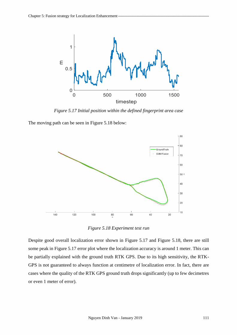
Chapter 5: Fusion strategy for Localization Enhancement -------------------------------------------------------------------------
Nguyen Dinh Van - January 2019 111
Figure 5.17 Initial position within the defined fingerprint area case
The moving path can be seen in Figure 5.18 below:
Figure 5.18 Experiment test run
Despite good overall localization error shown in Figure 5.17 and Figure 5.18, there are still
some peak in Figure 5.17 error plot where the localization accuracy is around 1 meter. This can
be partially explained with the ground truth RTK GPS. Due to its high sensitivity, the RTK-
GPS is not guaranteed to always function at centimetre of localization error. In fact, there are
cases where the quality of the RTK GPS ground truth drops significantly (up to few decimetres
or even 1 meter of error).
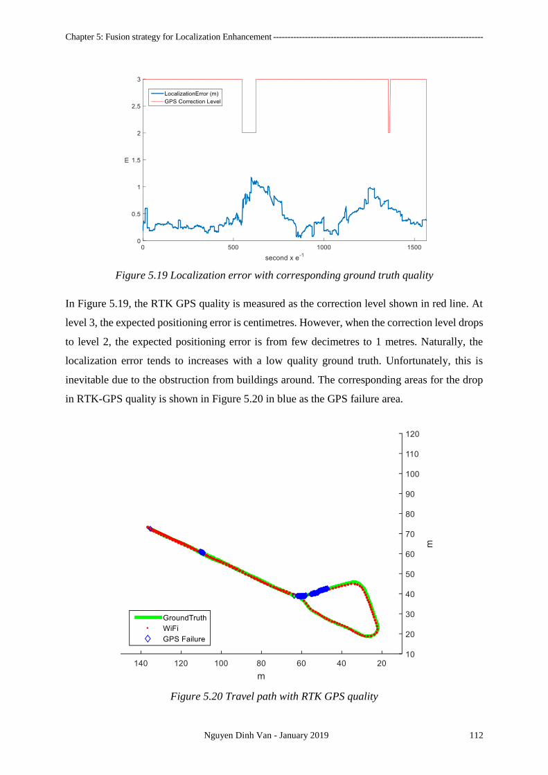
Chapter 5: Fusion strategy for Localization Enhancement -------------------------------------------------------------------------
Nguyen Dinh Van - January 2019 112
Figure 5.19 Localization error with corresponding ground truth quality
In Figure 5.19, the RTK GPS quality is measured as the correction level shown in red line. At
level 3, the expected positioning error is centimetres. However, when the correction level drops
to level 2, the expected positioning error is from few decimetres to 1 metres. Naturally, the
localization error tends to increases with a low quality ground truth. Unfortunately, this is
inevitable due to the obstruction from buildings around. The corresponding areas for the drop
in RTK-GPS quality is shown in Figure 5.20 in blue as the GPS failure area.
Figure 5.20 Travel path with RTK GPS quality
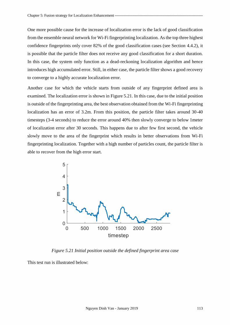
Chapter 5: Fusion strategy for Localization Enhancement -------------------------------------------------------------------------
Nguyen Dinh Van - January 2019 113
One more possible cause for the increase of localization error is the lack of good classification
from the ensemble neural network for Wi-Fi fingerprinting localization. As the top three highest
confidence fingerprints only cover 82% of the good classification cases (see Section 4.4.2), it
is possible that the particle filter does not receive any good classification for a short duration.
In this case, the system only function as a dead-reckoning localization algorithm and hence
introduces high accumulated error. Still, in either case, the particle filter shows a good recovery
to converge to a highly accurate localization error.
Another case for which the vehicle starts from outside of any fingerprint defined area is
examined. The localization error is shown in Figure 5.21. In this case, due to the initial position
is outside of the fingerprinting area, the best observation obtained from the Wi-Fi fingerprinting
localization has an error of 3.2m. From this position, the particle filter takes around 30-40
timesteps (3-4 seconds) to reduce the error around 40% then slowly converge to below 1meter
of localization error after 30 seconds. This happens due to after few first second, the vehicle
slowly move to the area of the fingerprint which results in better observations from Wi-Fi
fingerprinting localization. Together with a high number of particles count, the particle filter is
able to recover from the high error start.
Figure 5.21 Initial position outside the defined fingerprint area case
This test run is illustrated below:
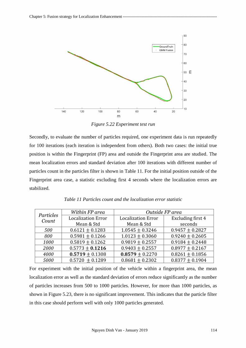
Chapter 5: Fusion strategy for Localization Enhancement -------------------------------------------------------------------------
Nguyen Dinh Van - January 2019 114
Figure 5.22 Experiment test run
Secondly, to evaluate the number of particles required, one experiment data is run repeatedly
for 100 iterations (each iteration is independent from others). Both two cases: the initial true
position is within the Fingerprint (FP) area and outside the Fingerprint area are studied. The
mean localization errors and standard deviation after 100 iterations with different number of
particles count in the particles filter is shown in Table 11. For the initial position outside of the
Fingerprint area case, a statistic excluding first 4 seconds where the localization errors are
stabilized.
Table 11 Particles count and the localization error statistic
Particles Count
Within FP area Outside FP area Localization Error
Mean & Std Localization Error
Mean & Std Excluding first 4
seconds 500 0.6121 ± 0.1283 1.0545 ± 0.3246 0.9457 ± 0.2827 800 0.5981 ± 0.1266 1.0123 ± 0.3060 0.9240 ± 0.2605
1000 0.5819 ± 0.1262 0.9819 ± 0.2557 0.9184 ± 0.2448 2000 0.5773 ± 0.1216 0.9403 ± 0.2557 0.8977 ± 0.2167 4000 0.5719 ± 0.1308 0.8579 ± 0.2270 0.8261 ± 0.1856 5000 0.5720 ± 0.1289 0.8681 ± 0.2302 0.8377 ± 0.1904
For experiment with the initial position of the vehicle within a fingerprint area, the mean
localization error as well as the standard deviation of errors reduce significantly as the number
of particles increases from 500 to 1000 particles. However, for more than 1000 particles, as
shown in Figure 5.23, there is no significant improvement. This indicates that the particle filter
in this case should perform well with only 1000 particles generated.
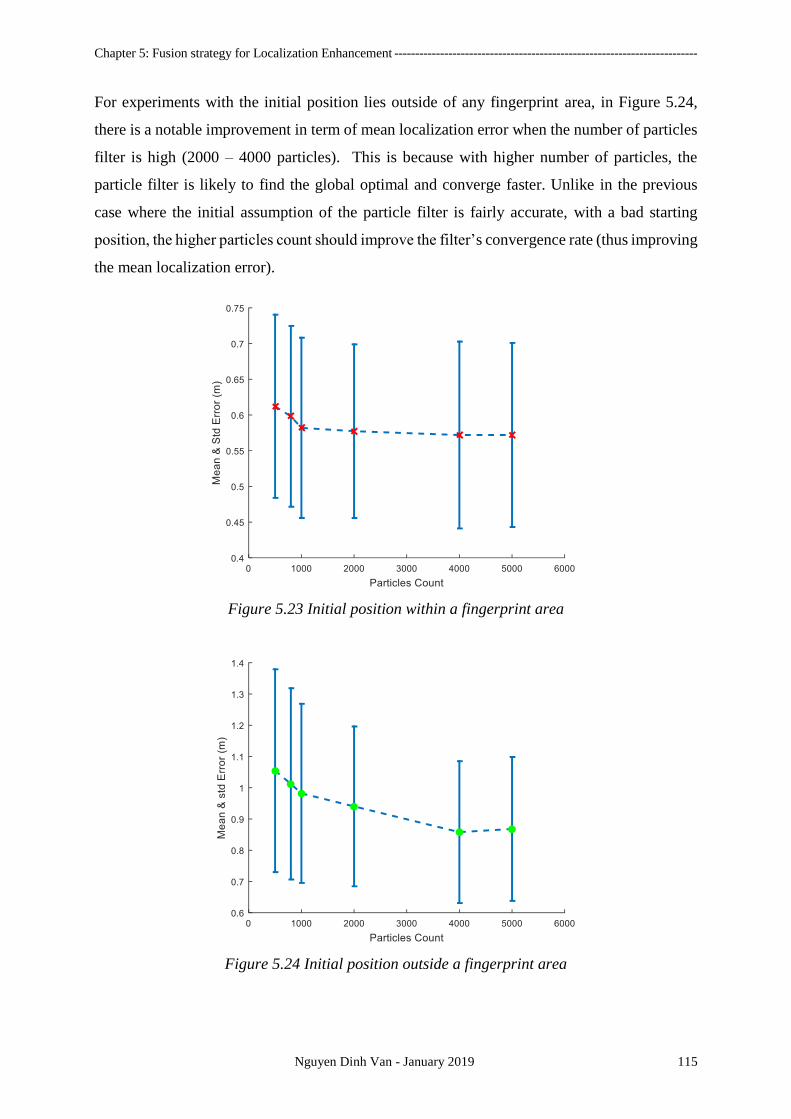
Chapter 5: Fusion strategy for Localization Enhancement -------------------------------------------------------------------------
Nguyen Dinh Van - January 2019 115
For experiments with the initial position lies outside of any fingerprint area, in Figure 5.24,
there is a notable improvement in term of mean localization error when the number of particles
filter is high (2000 – 4000 particles). This is because with higher number of particles, the
particle filter is likely to find the global optimal and converge faster. Unlike in the previous
case where the initial assumption of the particle filter is fairly accurate, with a bad starting
position, the higher particles count should improve the filter’s convergence rate (thus improving
the mean localization error).
Figure 5.23 Initial position within a fingerprint area
Figure 5.24 Initial position outside a fingerprint area
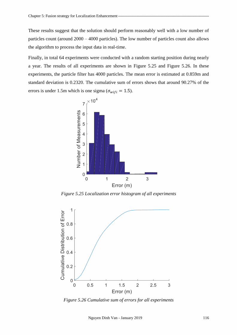
Chapter 5: Fusion strategy for Localization Enhancement -------------------------------------------------------------------------
Nguyen Dinh Van - January 2019 116
These results suggest that the solution should perform reasonably well with a low number of
particles count (around 2000 – 4000 particles). The low number of particles count also allows
the algorithm to process the input data in real-time.
Finally, in total 64 experiments were conducted with a random starting position during nearly
a year. The results of all experiments are shown in Figure 5.25 and Figure 5.26. In these
experiments, the particle filter has 4000 particles. The mean error is estimated at 0.859m and
standard deviation is 0.2320. The cumulative sum of errors shows that around 90.27% of the
errors is under 1.5m which is one sigma (𝜎𝑤𝑖𝑓𝑖 = 1.5).
Figure 5.25 Localization error histogram of all experiments
Figure 5.26 Cumulative sum of errors for all experiments
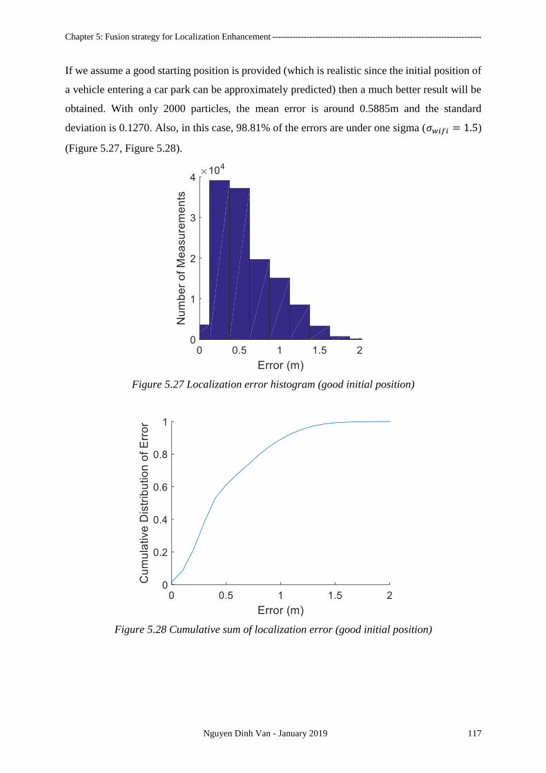
Chapter 5: Fusion strategy for Localization Enhancement -------------------------------------------------------------------------
Nguyen Dinh Van - January 2019 117
If we assume a good starting position is provided (which is realistic since the initial position of
a vehicle entering a car park can be approximately predicted) then a much better result will be
obtained. With only 2000 particles, the mean error is around 0.5885m and the standard
deviation is 0.1270. Also, in this case, 98.81% of the errors are under one sigma (𝜎𝑤𝑖𝑓𝑖 = 1.5)
(Figure 5.27, Figure 5.28).
Figure 5.27 Localization error histogram (good initial position)
Figure 5.28 Cumulative sum of localization error (good initial position)

Chapter 5: Fusion strategy for Localization Enhancement -------------------------------------------------------------------------
Nguyen Dinh Van - January 2019 118
5.6.2 Wi-Fi Fingerprinting Localization, IMU and Laser-SLAM fusion
5.6.2.1 Laser-SLAM in Global Coordinate Frame
In this solution, the transformation matrix needs first to be found using the RTK-GPS. However,
any small error in the estimation for the transformation matrix will be accumulated as the
vehicle moves further. In practice, even with the RTK-GPS, the resulted transformation matrix
would still suffer from noise. Figure 5.29 illustrates a test case for the conversion of the SLAM
local coordinate frame into the global coordinate frame. Even though the first 10 meters of the
moving path, the laser-SLAM result in global coordinates seem to be accurate, a rapid growth
in localization error could be seen afterward. There are two possible causes for this problem:
(1) an incorrect transformation matrix and (2) the accumulated error of the laser-SLAM itself
(or the drifting issue).
Figure 5.29 laser-SLAM in Global Coordinate
While it is possible that both sources of error above are true the accumulated error issue could
be fix with the injection of the Wi-Fi observation. Still, it is extremely difficult to deal with the
calculation of a transformation matrix issue in practice.
An attempt to fuse the Wi-Fi fingerprinting system into the SLAM (both Evidential SLAM and
PML SLAM) is made. The result of localization can be seen in Figure 5.30. Clearly, with the
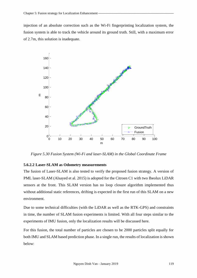
Chapter 5: Fusion strategy for Localization Enhancement -------------------------------------------------------------------------
Nguyen Dinh Van - January 2019 119
injection of an absolute correction such as the Wi-Fi fingerprinting localization system, the
fusion system is able to track the vehicle around its ground truth. Still, with a maximum error
of 2.7m, this solution is inadequate.
Figure 5.30 Fusion System (Wi-Fi and laser-SLAM) in the Global Coordinate Frame
5.6.2.2 Laser-SLAM as Odometry measurements
The fusion of Laser-SLAM is also tested to verify the proposed fusion strategy. A version of
PML laser-SLAM (Alsayed et al. 2015) is adopted for the Citroen C1 with two Ibeolux LiDAR
sensors at the front. This SLAM version has no loop closure algorithm implemented thus
without additional static references, drifting is expected in the first run of this SLAM on a new
environment.
Due to some technical difficulties (with the LiDAR as well as the RTK-GPS) and constraints
in time, the number of SLAM fusion experiments is limited. With all four steps similar to the
experiments of IMU fusion, only the localization results will be discussed here.
For this fusion, the total number of particles are chosen to be 2000 particles split equally for
both IMU and SLAM based prediction phase. In a single run, the results of localization is shown
below:
0 10 20 30 40 50 60 70 80 90 1000
20
40
60
80
100
120
140
160
m
m
GroundTruth
Fusion
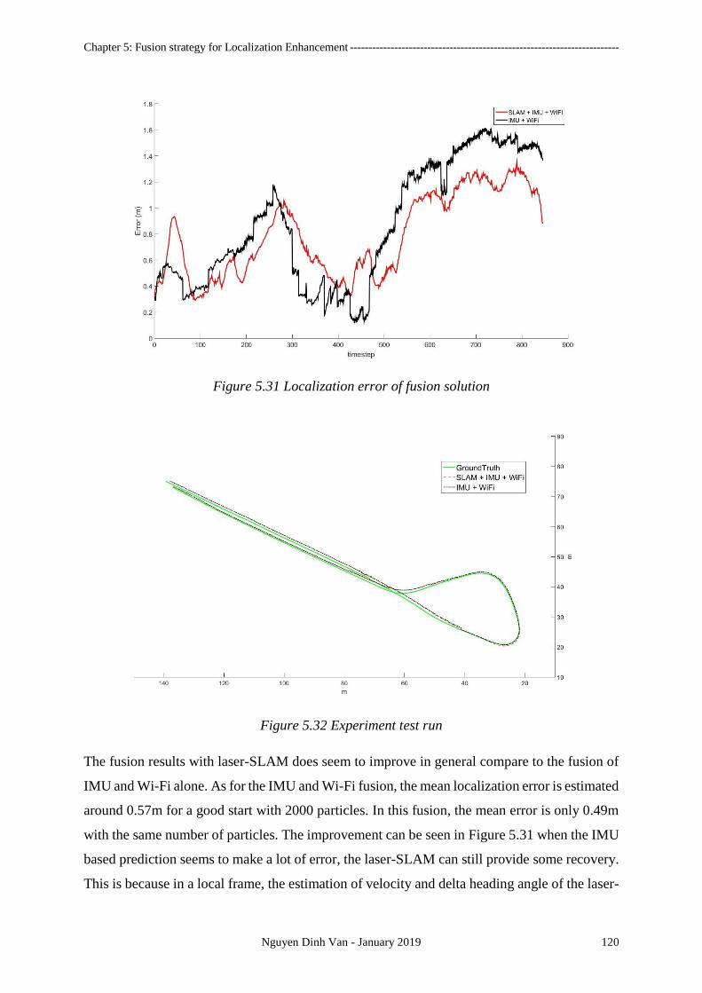
Chapter 5: Fusion strategy for Localization Enhancement -------------------------------------------------------------------------
Nguyen Dinh Van - January 2019 120
Figure 5.31 Localization error of fusion solution
Figure 5.32 Experiment test run
The fusion results with laser-SLAM does seem to improve in general compare to the fusion of
IMU and Wi-Fi alone. As for the IMU and Wi-Fi fusion, the mean localization error is estimated
around 0.57m for a good start with 2000 particles. In this fusion, the mean error is only 0.49m
with the same number of particles. The improvement can be seen in Figure 5.31 when the IMU
based prediction seems to make a lot of error, the laser-SLAM can still provide some recovery.
This is because in a local frame, the estimation of velocity and delta heading angle of the laser-
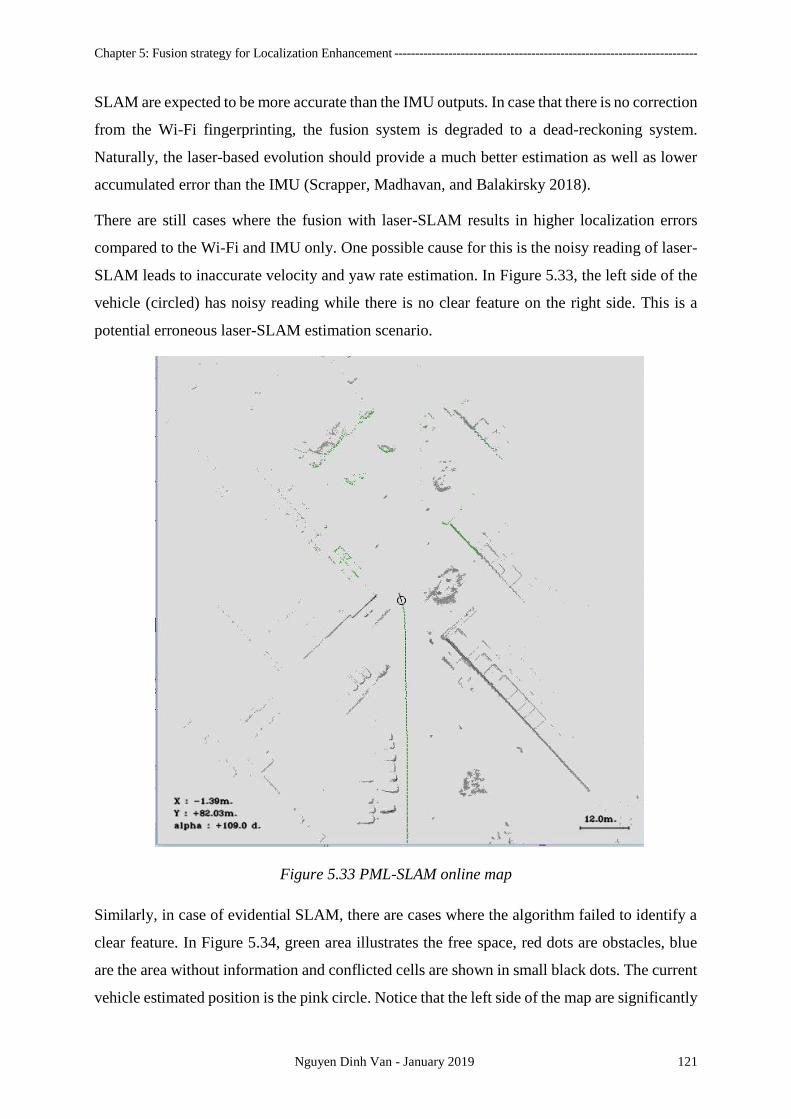
Chapter 5: Fusion strategy for Localization Enhancement -------------------------------------------------------------------------
Nguyen Dinh Van - January 2019 121
SLAM are expected to be more accurate than the IMU outputs. In case that there is no correction
from the Wi-Fi fingerprinting, the fusion system is degraded to a dead-reckoning system.
Naturally, the laser-based evolution should provide a much better estimation as well as lower
accumulated error than the IMU (Scrapper, Madhavan, and Balakirsky 2018).
There are still cases where the fusion with laser-SLAM results in higher localization errors
compared to the Wi-Fi and IMU only. One possible cause for this is the noisy reading of laser-
SLAM leads to inaccurate velocity and yaw rate estimation. In Figure 5.33, the left side of the
vehicle (circled) has noisy reading while there is no clear feature on the right side. This is a
potential erroneous laser-SLAM estimation scenario.
Figure 5.33 PML-SLAM online map
Similarly, in case of evidential SLAM, there are cases where the algorithm failed to identify a
clear feature. In Figure 5.34, green area illustrates the free space, red dots are obstacles, blue
are the area without information and conflicted cells are shown in small black dots. The current
vehicle estimated position is the pink circle. Notice that the left side of the map are significantly
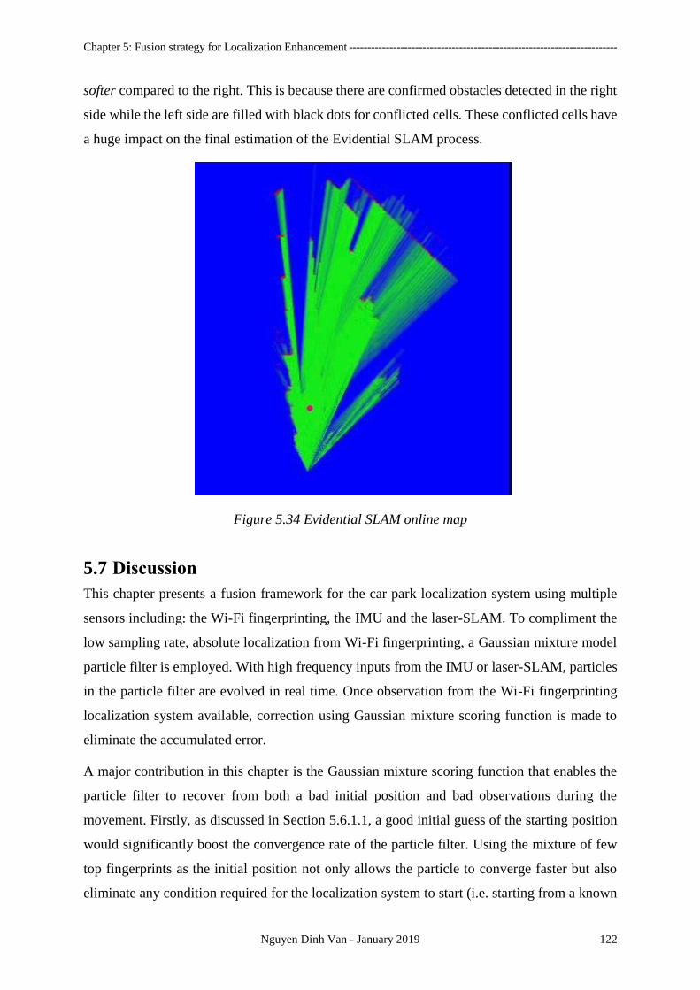
Chapter 5: Fusion strategy for Localization Enhancement -------------------------------------------------------------------------
Nguyen Dinh Van - January 2019 122
softer compared to the right. This is because there are confirmed obstacles detected in the right
side while the left side are filled with black dots for conflicted cells. These conflicted cells have
a huge impact on the final estimation of the Evidential SLAM process.
Figure 5.34 Evidential SLAM online map
5.7 Discussion
This chapter presents a fusion framework for the car park localization system using multiple
sensors including: the Wi-Fi fingerprinting, the IMU and the laser-SLAM. To compliment the
low sampling rate, absolute localization from Wi-Fi fingerprinting, a Gaussian mixture model
particle filter is employed. With high frequency inputs from the IMU or laser-SLAM, particles
in the particle filter are evolved in real time. Once observation from the Wi-Fi fingerprinting
localization system available, correction using Gaussian mixture scoring function is made to
eliminate the accumulated error.
A major contribution in this chapter is the Gaussian mixture scoring function that enables the
particle filter to recover from both a bad initial position and bad observations during the
movement. Firstly, as discussed in Section 5.6.1.1, a good initial guess of the starting position
would significantly boost the convergence rate of the particle filter. Using the mixture of few
top fingerprints as the initial position not only allows the particle to converge faster but also
eliminate any condition required for the localization system to start (i.e. starting from a known
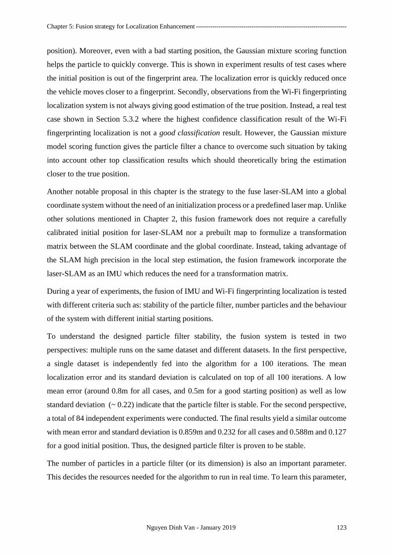
Chapter 5: Fusion strategy for Localization Enhancement -------------------------------------------------------------------------
Nguyen Dinh Van - January 2019 123
position). Moreover, even with a bad starting position, the Gaussian mixture scoring function
helps the particle to quickly converge. This is shown in experiment results of test cases where
the initial position is out of the fingerprint area. The localization error is quickly reduced once
the vehicle moves closer to a fingerprint. Secondly, observations from the Wi-Fi fingerprinting
localization system is not always giving good estimation of the true position. Instead, a real test
case shown in Section 5.3.2 where the highest confidence classification result of the Wi-Fi
fingerprinting localization is not a good classification result. However, the Gaussian mixture
model scoring function gives the particle filter a chance to overcome such situation by taking
into account other top classification results which should theoretically bring the estimation
closer to the true position.
Another notable proposal in this chapter is the strategy to the fuse laser-SLAM into a global
coordinate system without the need of an initialization process or a predefined laser map. Unlike
other solutions mentioned in Chapter 2, this fusion framework does not require a carefully
calibrated initial position for laser-SLAM nor a prebuilt map to formulize a transformation
matrix between the SLAM coordinate and the global coordinate. Instead, taking advantage of
the SLAM high precision in the local step estimation, the fusion framework incorporate the
laser-SLAM as an IMU which reduces the need for a transformation matrix.
During a year of experiments, the fusion of IMU and Wi-Fi fingerprinting localization is tested
with different criteria such as: stability of the particle filter, number particles and the behaviour
of the system with different initial starting positions.
To understand the designed particle filter stability, the fusion system is tested in two
perspectives: multiple runs on the same dataset and different datasets. In the first perspective,
a single dataset is independently fed into the algorithm for a 100 iterations. The mean
localization error and its standard deviation is calculated on top of all 100 iterations. A low
mean error (around 0.8m for all cases, and 0.5m for a good starting position) as well as low
standard deviation (~ 0.22) indicate that the particle filter is stable. For the second perspective,
a total of 84 independent experiments were conducted. The final results yield a similar outcome
with mean error and standard deviation is 0.859m and 0.232 for all cases and 0.588m and 0.127
for a good initial position. Thus, the designed particle filter is proven to be stable.
The number of particles in a particle filter (or its dimension) is also an important parameter.
This decides the resources needed for the algorithm to run in real time. To learn this parameter,
Chapter 5: Fusion strategy for Localization Enhancement -------------------------------------------------------------------------
Nguyen Dinh Van - January 2019 124
different number of particles are tested in the same dataset. Finally, with only 2000 particles,
the fusion solution is able to achieve the optimal result.
Different initial positions for test runs are also studied to understand the generalization of the
algorithm. There are two possibilities for place for the initial position: either within or outside
a fingerprint area. If the initial position is within a fingerprint area, a good initial guess can be
expected. This results in a low mean localization error of 0.588m. Otherwise, since the particle
filter needs time to converge to the true position, the mean localization error in this case is
around 0.859m. This high mean error is mostly due to the initial large positioning error. In
addition, it is reasonable to expect the initial position of a vehicle entering a car park is relatively
known. Hence, a good accuracy can be expected from the fusion system in general.
Although, the average movement speed in all experiments is around 3.3m/s, there is a
possibility of extending the thesis result to a higher movement speed. In order to accomplish
this, a solution to enhance Wi-Fi fingerprinting localization sampling frequency must be found.
One potential way is to use multiple Wi-Fi antenna with different processors, each has a small
delay to the other. In this way, the sampling frequency of Wi-Fi scan can be increased
proportional to the number of antennas. Unfortunately, with limited time, the thesis could not
be extended to cover the idea.
Finally, the proposed fusion framework allows not only the fusion of Wi-Fi fingerprinting with
other sensors but it has the potential to combine different strategies such as the GPS with laser-
SLAM, GPS with camera-based localization system, etc.. With that being said, this framework
can be applied to multiple scenarios but not just GPS-denied environment or car park.

Chapter 5: Fusion strategy for Localization Enhancement -------------------------------------------------------------------------
Nguyen Dinh Van - January 2019 125
126
6. CONCLUSION
Résumé
Le chapitre conclut la thèse avec deux contributions majeures et une perspective pour les
travaux futurs. Après avoir défini le problème au début, une solution basée sur le réseau de
capteurs sans fil est proposée. Le chapitre 4 explique pourquoi un système de localisation
d'empreintes digitales Wi-Fi peut répondre aux quatre critères. À condition que, un réseau de
neurones d'ensemble pour l'empreinte Wi-Fi est proposé. La base de données hybride
d'empreintes digitales et un réseau de neurones d'ensemble destinés à aider la localisation
d'empreintes digitales Wi-Fi à s'adapter à la circulation d'un véhicule dans un parking sont deux
contributions majeures. Des expériences sur des véhicules réels ont été menées pendant une
année pour valider le système proposé. Avec deux véhicules différents, 64 expériences, le
système fournit une erreur de localisation moyenne de 2,25 m. Cela prouve que le système de
localisation d'empreintes digitales Wi-Fi proposé est capable de remplacer le GPS dans un
environnement sans GPS.
Toutefois, comme indiqué dans le champ d’application, l’erreur de localisation souhaitée pour
un véhicule intelligent est d’environ 0,2 m. De plus, le système devrait pouvoir localiser le
véhicule à haute fréquence pour faire face aux mouvements à grande vitesse. Par conséquent,
un cadre de fusion pour la localisation d'empreintes digitales Wi-Fi et un autre système tel que
l'IMU ou le laser-SLAM est proposé. L’objectif de ces systèmes est d’améliorer
progressivement la fréquence de localisation, la précision et la transition de l’environnement
assisté par GPS à un environnement refusé par GPS. Afin d'accomplir cette tâche, le filtre de
Chapter 6: Conclusion ---------------------------------------------------------------------------------------------------------------------
Nguyen Dinh Van - January 2019 127
particules d'amorçage, une méthode de filtrage non linéaire est choisie. Comparé à un autre
algorithme de filtrage, le filtre à particules semble offrir de meilleures performances en matière
d’estimation non linéaire. En général, l'étape de correction du filtre à particules prendra en
compte les observations disponibles pour peser sur l'ensemble candidat de positionnement (ou
les particules). Compte tenu des observations absolues de méthodes telles que la localisation
GPS, par caméra ou Wi-Fi, la meilleure estimation est souvent prise en compte pour évaluer
l'ensemble de positionnement candidat. Dans cette thèse, la correction est prise à partir du
système de localisation d'empreintes digitales Wi-Fi. Avec une étude statistique du chapitre 4,
il est justifié que les 3 premiers résultats de la classification donnent une bien meilleure
estimation de la position réelle que seulement le score le plus élevé. Par conséquent, au lieu de
considérer uniquement le score de confiance le plus élevé du résultat de la localisation Wi-Fi,
le filtre prend en compte plusieurs scores possibles (3 en haut dans cette thèse) sous forme
d'observations. Une fonction de notation utilisant un modèle de mélange gaussien de ces
observations est définie. Les avantages de cette approche sont décrits à la section 5.3.
Parmi les différents capteurs, deux des capteurs les plus courants pour véhicules autonomes
sont choisis pour la fusion dans cette thèse, à savoir l'unité de mesure inertielle (IMU) et le
LiDAR. Bien qu'il s'agisse d'un couplage standard du GPS et du LiDAR (ou Velodyme) dans
l'environnement assisté par GPS pour la localisation précise de véhicules intelligents, ce n'est
pas le cas pour l'environnement assisté par GPS. Ainsi, une combinaison de la localisation Wi-
Fi et du SLAM laser est proposée. À ce jour, le travail de thèse est également la première
tentative de fusion de la localisation Wi-Fi et du laser-SLAM pour le positionnement de
véhicules autonomes. Les détails de la stratégie de fusion sont expliqués au chapitre 5.
Enfin, avec de plus en plus d'études sur le même sujet chaque année, l'auteur estime que la
solution de localisation de réseaux de capteurs sans fil deviendrait éventuellement une solution
mature pour le positionnement de véhicules intelligents dans des environnements intérieurs.
6.1 Thesis motivation
In this thesis, the author has introduced the motivation to solve the localization problem of
intelligent vehicles in the GPS-denied environment, especially a car park. The thesis pointed
out that by having an autonomous navigation system for vehicles, an approximately 700 million
euros loss can be avoided for France alone. Reports show that approximately 62% of carpark
space will be saved if all vehicles are autonomously parked. In addition, car parks uses are

Chapter 6: Conclusion ---------------------------------------------------------------------------------------------------------------------
Nguyen Dinh Van - January 2019 128
increasingly exceeding their original purpose. Features such as electric chargers for electric
cars, online booking of parking spaces, dynamic guidance, etc. are growing demands. As France
is committed to a digital Republic by October 2018, this thesis is expected to be a timely
solution for environments such as car park.
However, a throughout study of literature for car park localization of intelligent vehicles does
not seems to agree on a single architecture. It does, however, emphasize the need for an absolute
correction system to couple with another dead-reckoning algorithm for the GPS-denied
environment. Workarounds including laser or camera based SLAM, vision map matching or
geo-referencing of environment landmarks are proposed with promising results. Still, these
solutions do not comply with four criteria of a universal solution: availability, scalability,
universal and accuracy. More specifically, most of the solutions violate the scalability and
universal criteria as a costly mapping (and maintaining) process is required, or dedicated
sensors calibration needed. On a large-scale, dynamic environments where changes happen
every day, these costly procedures are soon to be a huge burden on the entire system.
In addition, with the growth of the wireless sensors networks infrastructure, it is interesting to
investigate a possible solution using these readily available sensors to locate intelligent
vehicles. Furthermore, from the beginning of 2017, the research community for indoor
localization system using wireless sensors networks starts to address the autonomous driving
problem for indoor environments. Notable conferences such as IPIN (Indoor Positioning and
Indoor Navigation), the Microsoft indoor localization competition IPSN are embracing the idea
of preparing and developing a navigation system for vehicles in indoor environments. Still,
works on this topic are far from reaching the system requirements as pointed out in Section 4.2.
6.2 Thesis contributions
Having defined the problem and its requirements, a solution based on Wireless Sensors
Network is proposed. Chapter 4 gives a discussion on why a Wi-Fi fingerprinting localization
system could satisfy all four criteria. Provided that, an ensemble neural network for Wi-Fi
fingerprinting is proposed. Two major contributions are the hybrid database of fingerprints as
well as an ensemble neural network to help the Wi-Fi fingerprinting localization adapt to a
vehicle movement inside a car park. Experiments on real vehicles were conducted for a duration
of one year to validate the proposed system. With two different vehicles, 64 experiments, the
system provides a 2.25m of average localization error. This proves that the proposed Wi-Fi
Chapter 6: Conclusion ---------------------------------------------------------------------------------------------------------------------
Nguyen Dinh Van - January 2019 129
fingerprinting localization system is capable of replacing the GPS in a GPS-denied
environment.
Still, as stated in the scope, the desired localization error for an intelligent vehicle is around
0.2m. In addition, the system should be able to locate the vehicle in high frequency to cope with
high-speed movement. Therefore, a fusion framework for the Wi-Fi fingerprinting localization
and another system such as the IMU or laser-SLAM is proposed. The goal of such systems is
to smoothly improve localization frequency, accuracy as well as the transition from the GPS-
aided environment to GPS-denied environment. In order to accomplish the task, the bootstrap
particle filter, a non-linear filtering method is chosen. Compare to other filtering algorithm, the
particle filter appears to have better performance when it comes to non-linear estimation. In
general, the correction step of the particle filter will take into account available observations to
put weight on the positioning candidate set (or the particles). Given absolute observations from
methods such as GPS, camera or Wi-Fi localization, often, the best estimation is taken into
account evaluate the positioning candidate set. In this thesis, the correction is taken from the
Wi-Fi fingerprinting localization system. Having a statistic study from Chapter 4, it is justified
that the top 3 classification results give a much better estimation of the true position than only
the highest score one. Hence, instead of considering just the highest confidence score from the
Wi-Fi localization result, the filter takes into account multiple possible ones (3-top in this thesis)
as observations. A scoring function using Gaussian mixture model of those observations is
defined. The benefit of this approach is described in Section 5.3.
Among different sensors, two of the most common ones for autonomous vehicles are chosen
for fusion in this thesis namely the Inertial Measurement Unit (IMU) and LiDAR. While it is a
standard coupling of the GPS and LiDAR (or Velodyme) in the GPS-aided environment for the
precise localization of intelligent vehicles, it is not the case for the GPS-aided environment.
Thus, a combination of the Wi-Fi localization and the laser-based SLAM is proposed. To this
date, the thesis work is also the first attempt to fuse the Wi-Fi localization and the laser-SLAM
for autonomous vehicles positioning. Details of the fusion strategy is explained in Chapter 5.
Since the particle filter is non-deterministic process, it is important to study the stability as well
as the accuracy of the framework. There are two ways to analyze: to iterate the algorithm on
the same dataset multiple times and to test the algorithm on different datasets. The first way is
to understand the behaviour of the particle filter on the same dataset in different run. If the
results of multiple runs agree on the same accuracy, it is likely that the particle filter is stable.
The second way is to explore the particle filter reaction to different datasets. Given different

Chapter 6: Conclusion ---------------------------------------------------------------------------------------------------------------------
Nguyen Dinh Van - January 2019 130
conditions and testing data, the particle filter should also deliver a stable result. In total, there
are 64 different datasets for the fusion of Wi-Fi, IMU and laser-SLAM. Each of these datasets
is repeatedly fed into the fusion framework for 100 times. Finally, given a good starting
condition (which is expected for a vehicle when entering a car park, its first initial position is
predicted), the system accuracy is around 0.58m with a low standard deviation of 0.12.
Although such accuracy is still far from the desired one, it is important to note that this accuracy
is calculated on the global coordinate system. Hence, further fine-tuning can be expected within
local localization level (such as laser, camera, etc.).
6.3 Future work
Until now, most of commercial systems for carpark navigation from companies like BMW,
Volvo, etc. are demonstrating at a low speed (around 3m/s). The survey from (Belloche 2015)
also confirmed that the average speed for vehicles inside carparks is around 3-4m/s. However,
the demand for a higher speed of navigation is expected in the future when the infrastructure
and the transportation agents (vehicles, drivers, etc.) are ready. The benefit of such high speed
navigation is obvious as it will increase the transportation flows vastly. Even though the study
in the thesis focuses on a car park with an average speed of 3.3m/s, a potential solution for
higher speed movement is also discussed in Section 5.7. With multiple Wi-Fi antennas to
enhance the Wi-Fi sampling rate, it is possible that the fusion solution can localize vehicles at
a higher speed. The future work of this thesis will study the possibility of pushing the navigation
speed to a new limit.
Also, it is highly likely that an HD (high definition) map of the environment captured by sensors
such as LIDAR or camera is eventually needed for centimetre level of positioning accuracy.
Should the map is ready, the work in this thesis is believed to maintain a major impact. There
are three reasons for this. First, with only an IMU and the Wi-Fi system, this thesis can provide
an excellent loop-closure detection mechanism for the SLAM process in its initial map
recording. More often, the SLAM tends to drift in its first run. This drift leads to a potential
failure to close the loop on the map when the vehicle returns to the starting point. In this case,
an absolute correction is required to help to reduce the accumulated error and to detect the
previously visited area. Second, the fusion framework in this thesis can be extended to multiple
sensors and localization systems such as camera, magnetic, ultra-wideband, etc. The concept of
Gaussian mixture model allows the framework to incorporate information from different
sources for a better estimation. Finally, having redundancy for a critical system such as
Chapter 6: Conclusion ---------------------------------------------------------------------------------------------------------------------
Nguyen Dinh Van - January 2019 131
positioning for intelligent vehicles is extremely important. In unexpected situations, even the
pre-recorded HD map approach could fail to locate the vehicle (or worse, return a huge
positioning error). The IMU and Wi-Fi fusion could then be used as an anomaly detection in
those situations and provide relatively accurate positioning information for the vehicle.
In the near future, a more comprehensive study of the proposed system is expected. Ideas such
as multiple antennas, anomaly detection for map-based methods or the fusion with laser/camera
based SLAM are among possible research directions. Special techniques such as Channel State
Information (CSI) for reading the Wi-Fi information to replace the unstable RSSIs could also
be exploited as hardware becomes more and more available. The combination of those ideas
could lead to a considerable improvement in the Wi-Fi, IMU and SLAM fusion system
accuracy.
Regarding the carpark situation, the absolute localization approach in this thesis brings an
opportunity for location-based context aware services such as mobile payment, parking slot
reservation, car-finding and charging station for electric vehicles. Moreover, the author also
hopes to apply the proposed framework for other scenarios such as indoor robots navigation,
vehicle navigation in industrial warehouses, or university campus buses. Each of these
scenarios, however, will have different requirements (i.e. average movement speed, localization
accuracy requirement, power consumption level or deployment cost, etc.). The author believes
that the proposed system could be deployed effortlessly for those scenarios given the flexibility
of the fusion framework.
Not only that more Wi-Fi access points are naturally added to the environment, the quality of
these off the shelf, but consumer-grade hardware are also becoming better and better. While
technologies such as Bluetooth Low Energy (BLE), ultra-wideband or 5G were not even
mentioned ten years ago, they now can all be integrated in the indoor localization system. This
shows that a potential of replacing the GPS with wireless sensor networks for indoor or even
urban area is high. Besides, with more and more studies are being found in the same topic each
year, the author believes that the wireless sensor networks localization solution would
eventually be a mature solution for intelligent vehicles positioning in the indoor environments.
6.4 Conclusion
In conclusion, the thesis proposes a fusion system for localizing intelligent vehicles in the GPS-
denied environment, more specifically the carpark situation. The practical necessity of the
problem is explained in Chapter 1. It is reported that by accomplishing the task of autonomous
Chapter 6: Conclusion ---------------------------------------------------------------------------------------------------------------------
Nguyen Dinh Van - January 2019 132
navigation for vehicles in carpark, there will be a huge benefit economically. While the existing
solutions are not fully address the problem (or not cost-effective), the literature review in
Chapter 2 does not yield a complete solution as well. By identifying four major criteria for the
system, a fusion framework of Wi-Fi fingerprinting localization, IMU and laser-SLAM are
designed. Experiments show promising results with room for improvement in the future.
Chapter 7: References ---------------------------------------------------------------------------------------------------------------------
Nguyen Dinh Van - January 2019 133
7. REFERENCES
Abdallah, Ali A., Samer S. Saab, and Zaher M. Kassas. 2018. “A Machine Learning Approach
for Localization in Cellular Environments.” In 2018 IEEE/ION Position, Location and
Navigation Symposium (PLANS), 1223–27. IEEE. doi:10.1109/PLANS.2018.8373508.
Agamennoni, Gabriel, Simone Fontana, Roland Y Siegwart, and Domenico G Sorrenti. 2016.
“Point Clouds Registration with Probabilistic Data Association.” Proceedings of the
IEEE/RSJ International Conference on Intelligent Robots and Systems (IROS), 4092–98.
doi:10.1109/IROS.2016.7759602.
Agashe, Anil a., Amrita a. Agashe, and R.S. Patil. 2012. “Evaluation of DV Hop Localization
Algorithm in Wireless Sensor Networks.” 2012 International Conference on Advances in
Mobile Network, Communication and Its Applications, 79–82.
doi:10.1109/MNCApps.2012.21.
Akai, Naoki, Luis Yoichi Morales, Takuma Yamaguchi, Eijiro Takeuchi, Yuki Yoshihara,
Hiroyuki Okuda, Tatsuya Suzuki, and Yoshiki Ninomiya. 2017. “Autonomous Driving
Based on Accurate Localization Using Multilayer LiDAR and Dead Reckoning.” In 2017
IEEE 20th International Conference on Intelligent Transportation Systems (ITSC), 1–6.
IEEE. doi:10.1109/ITSC.2017.8317797.
Alarifi, Abdulrahman, AbdulMalik Al-Salman, Mansour Alsaleh, Ahmad Alnafessah, Suheer
Al-Hadhrami, Mai A Al-Ammar, and Hend S Al-Khalifa. 2016. “Ultra Wideband Indoor
Positioning Technologies: Analysis and Recent Advances.” Sensors (Basel, Switzerland)
16 (5). Multidisciplinary Digital Publishing Institute (MDPI). doi:10.3390/s16050707.
Alsayed, Zayed, Guillaume Bresson, Fawzi Nashashibi, and Anne Verroust-blondet. 2015.
“PML-SLAM : A Solution for Localization in Large-Scale Urban Environments.” IROS
PPNIV the 7th Workshop on Planning, Perception and Navigation for Intelligent Vehicles.
Amini, Arghavan, Reza Monir Vaghefi, Jesus M De Garza, and R Michael Buehrer. 2014.
“Improving GPS-Based Vehicle Positioning for Intelligent Transportation Systems,” no.
Iv: 1023–29.
Anderson, Frank C., and Marcus G. Pandy. 2001. “Dynamic Optimization of Human Walking.”
Journal of Biomechanical Engineering 123 (5): 381. doi:10.1115/1.1392310.
Chapter 7: References ---------------------------------------------------------------------------------------------------------------------
Nguyen Dinh Van - January 2019 134
Ang, Chee-wei. 2018. “Vehicle Positioning Using WIFI Fingerprinting in Urban
Environment.” In 2018 IEEE 4th World Forum on Internet of Things (WF-IoT), 4th:652–
57. doi:10.1109/WF-IoT.2018.8355136.
Arulampalam, M. Sanjeev, Simon Maskell, Neil Gordon, and Tim Clapp. 2007. “A Tutorial on
Particle Filters for Online Nonlinear/Nongaussian Bayesian Tracking.” Bayesian Bounds
for Parameter Estimation and Nonlinear Filtering/Tracking 50 (2): 723–37.
doi:10.1109/9780470544198.ch73.
Bar-Shalom, Yaakov, X.-Rong Li, and Thiagalingam Kirubarajan. 2001. Estimation with
Applications to Tracking and Navigation. New York, USA: John Wiley & Sons, Inc.
doi:10.1002/0471221279.
Belagiannis, Vasileios, Christian Rupprecht, Gustavo Carneiro, and Nassir Navab. 2015.
“Robust Optimization for Deep Regression.” Proceedings of the IEEE International
Conference on Computer Vision 2015 Inter: 2830–38. doi:10.1109/ICCV.2015.324.
Belloche, Sylvain. 2015. “On-Street Parking Search Time Modelling and Validation with
Survey-Based Data.” Transportation Research Procedia 6 (June 2014). Elsevier B.V.:
313–24. doi:10.1016/j.trpro.2015.03.024.
Besl, P.J., and Neil D. McKay. 1992. “A Method for Registration of 3-D Shapes.” IEEE
Transactions on Pattern Analysis and Machine Intelligence 14 (2): 239–56.
doi:10.1109/34.121791.
Bhatt, Deepak, Swarna Ravindra Babu, and Haresh S. Chudgar. 2017. “A Novel Approach
towards Utilizing Dempster Shafer Fusion Theory to Enhance WiFi Positioning System
Accuracy.” Pervasive and Mobile Computing 37. Elsevier B.V.: 115–23.
doi:10.1016/j.pmcj.2016.06.014.
Blumenthal, Jan, Ralf Grossmann, Frank Golatowski, and Dirk Timmermann. 2007. “Weighted
Centroid Localization in Zigbee-Based Sensor Networks.” In 2007 IEEE International
Symposium on Intelligent Signal Processing, 1–6. IEEE.
doi:10.1109/WISP.2007.4447528.
Bojja, J., M. Kirkko-Jaakkola, J. Collin, and J. Takala. 2013. “Indoor Localization Methods
Using Dead Reckoning and 3D Map Matching.” Journal of Signal Processing Systems, 1–
12. doi:10.1007/s11265-013-0865-9.
Borenstein, Johann. 1995. “Internal Correction of Dead-Reckoning Errors With a Dual-Drive
Chapter 7: References ---------------------------------------------------------------------------------------------------------------------
Nguyen Dinh Van - January 2019 135
Compliant Linkage Mobile Robot.” Reprint from Journal of Robotic Systems 12 (4): 257–
73. http://www-personal.umich.edu/~johannb/Papers/paper48.pdf.
Borges, Paulo, Robert Zlot, Michael Bosse, Stephen Nuske, and Ashley Tews. 2010. “Vision-
Based Localization Using an Edge Map Extracted from 3D Laser Range Data.” 2010 IEEE
International Conference on Robotics and Automation, 4902–9.
doi:10.1109/ROBOT.2010.5509517.
Boucher, Maxime, Fakhr-Eddine Ababsa, and Malik Mallem. 2013. “Reducing the SLAM Drift
Error Propagation Using Sparse but Accurate 3D Models for Augmented Reality
Applications.” In Proceedings of the Virtual Reality International Conference on Laval
Virtual - VRIC ’13, 1. New York, New York, USA: ACM Press.
doi:10.1145/2466816.2466828.
Boushaba, Mustapha, Abdelhakim Hafid, and Abderrahim Benslimane. 2009. “High Accuracy
Localization Method Using AoA in Sensor Networks.” Computer Networks 53 (18).
Elsevier B.V.: 3076–88. doi:10.1016/j.comnet.2009.07.015.
Box, G. E. P., and Mervin E. Muller. 1958. “A Note on the Generation of Random Normal
Deviates.” The Annals of Mathematical Statistics 29 (2). Institute of Mathematical
Statistics: 610–11. doi:10.1214/aoms/1177706645.
Breiman, Leo. 1996. “Bagging Predictors.” Machine Learning 24: 123–40.
doi:10.1007/BF00058655.
Bresson, Guillaume, Zayed Alsayed, Li Yu, and Sebastien Glaser. 2017. “Simultaneous
Localization And Mapping: A Survey of Current Trends in Autonomous Driving.” IEEE
Transactions on Intelligent Vehicles, 1–1. doi:10.1109/TIV.2017.2749181.
Bresson, Guillaume, Romuald Aufr, Roland Chapuis, Guillaume Bresson, Romuald Aufr,
Guillaume Bresson, and Romuald Aufr. 2016. “Improving SLAM with Drift Integration
To Cite This Version :”
Caffery, J.J. 2000. “A New Approach to the Geometry of TOA Location.” Vehicular
Technology Conference Fall 2000. IEEE VTS Fall VTC2000. 52nd Vehicular Technology
Conference (Cat. No.00CH37152) 4: 1943–49. doi:10.1109/VETECF.2000.886153.
Calvet, Laurent E., Veronika Czellar, and Elvezio Ronchetti. 2015. “Robust Filtering.” Journal
of the American Statistical Association 110 (512): 1591–1606.
doi:10.1080/01621459.2014.983520.

Chapter 7: References ---------------------------------------------------------------------------------------------------------------------
Nguyen Dinh Van - January 2019 136
Carlson, Justin, Charles Thorpe, and Brett Browning. 2010. “Mapping Large , Urban
Environments with GPS-Aided SLAM.”
Chen, Hongyang, Pei Huang, Marcelo Martins, Hing Cheung So, and Kaoru Sezaki. 2008.
“Novel Centroid Localization Algorithm for Three-Dimensional Wireless Sensor
Networks.” In 2008 4th International Conference on Wireless Communications,
Networking and Mobile Computing, 1–4. IEEE. doi:10.1109/WiCom.2008.841.
Chen, Huijie, Fan Li, and Yu Wang. 2018. “SoundMark: Accurate Indoor Localization via Peer-
Assisted Dead Reckoning.” IEEE Internet of Things Journal, 1–1.
doi:10.1109/JIOT.2018.2821364.
Chen, Shaojian, Zihao Li, and Yunliang Long. 2017. “An Adaptive Hybrid Indoor WiFi
Fingerprinting and Propagation Parameter Estimation Using RANSAC LASSO
Regression.” In 2017 IEEE 5th International Symposium on Electromagnetic
Compatibility (EMC-Beijing), 1–6. IEEE. doi:10.1109/EMC-B.2017.8260398.
Dao, Trung Kien, Hung Long Nguyen, Thanh Thuy Pham, Eric Castelli, Viet Tung Nguyen,
and Dinh Van Nguyen. 2014. “User Localization in Complex Environments by
Multimodal Combination of GPS, WiFi, RFID, and Pedometer Technologies.” The
Scientific World Journal 2014. ScientificWorld Ltd. doi:10.1155/2014/814538.
Daum, Fred. 2005. “Nonlinear Filters: Beyond the Kalman Filter.” IEEE Aerospace and
Electronic Systems Magazine 20 (8 II): 57–68. doi:10.1109/MAES.2005.1499276.
Daum, Fred, Jim Huang, and A Noushin. 2011. “Particle Flow for Nonlinear Filters.”
Proceedings of SPIE, 5920–23.
http://link.aip.org/link/?PSISDG/7697/769704/1%5Cnhttp://ieeexplore.ieee.org/xpls/abs
_all.jsp?arnumber=5947709.
De Ponte Müller, Fabian, Estefanía Munoz Diaz, and Ibrahim Rashdan. 2017. “Cooperative
Infrastructure-Based Vehicle Positioning.” IEEE Vehicular Technology Conference.
doi:10.1109/VTCFall.2016.7880941.
Dellaert, F., D. Fox, W. Burgard, and S. Thrun. 2018. “Monte Carlo Localization for Mobile
Robots.” In Proceedings 1999 IEEE International Conference on Robotics and
Automation (Cat. No.99CH36288C), 2:1322–28. IEEE. Accessed May 29.
doi:10.1109/ROBOT.1999.772544.
Department Of Defense, U.S.a. 2008. “Global Positioning System Standard Positioning

Chapter 7: References ---------------------------------------------------------------------------------------------------------------------
Nguyen Dinh Van - January 2019 137
Service.” Www.Gps.Gov, no. September: 1–160. http://www.gps.gov/technical/ps/2008-
SPS-performance-standard.pdf.
Dietterich, Thomas G. 2000. “Ensemble Methods in Machine Learning.” Multiple Classifier
Systems 1857: 1–15. doi:10.1007/3-540-45014-9.
“Differential GNSS - Navipedia.” 2018. Accessed May 27.
http://www.navipedia.net/index.php/Differential_GNSS.
Dongliang Huang, and H. Leung. 2004. “EM-IMM Based Land-Vehicle Navigation with
GPS/INS.” Proceedings. The 7th International IEEE Conference on Intelligent
Transportation Systems (IEEE Cat. No.04TH8749), no. Cv: 624–29.
doi:10.1109/ITSC.2004.1398973.
Douc, Randal, Olivier Cappé, and Eric Moulines. 2005. “Comparison of Resampling Schemes
for Particle Filtering,” 1–10. doi:10.1109/ISPA.2005.195385.
Doucet, Arnaud, and Adam M. Johansen. 2011. “A Tutorial on Particle Filtering and
Smoothing: Fiteen Years Later.” The Oxford Handbook of Nonlinear Filtering, no.
December 2008: 656–705. doi:10.1.1.157.772.
Drawil, Nabil Mohamed, and Otman Basir. 2010. “Intervehicle-Communication-Assisted
Localization” 11 (3): 678–91.
Drew Bagnell. 2018. “Particle Filter: The Good, The Bad, The Ugly.” Accessed August 5.
http://en.wikipedia.org/w/index.php?title=Stochastic_universal_sampling&oldid=356360
569.
Durrant-Whyte, H, and T Bailey. 2006. “Simultaneous Localization and Mapping (SLAM).”
IEEE Robotics & Automation Magazine 13 (2): 99–116.
doi:10.1109/MRA.2006.1638022.
Efron, Bradley., and Robert. Tibshirani. 1994. An Introduction to the Bootstrap. New York
N.Y. ;;London: Chapman & Hall. http://www.worldcat.org/title/introduction-to-the-
bootstrap/oclc/797437299.
El Faouzi, N.-E. 1997. “Heterogeneous Data Source Fusion for Impedance Indicators.” IFAC
Proceedings Volumes 30 (8). Elsevier: 1307–12. doi:10.1016/S1474-6670(17)44002-X.
Elfes, A. 2013. “Occupancy Grids: A Stochastic Spatial Representation for Active Robot
Perception,” March. http://arxiv.org/abs/1304.1098.
Chapter 7: References ---------------------------------------------------------------------------------------------------------------------
Nguyen Dinh Van - January 2019 138
Eskandarian, Azim. 2012. Handbook of Intelligent Vehicles. Springer.
F.~Gustafsson. 2010. “Particle Filter Theory and Practice with Positioning Applications.” IEEE
Transactions on Aerospace and Electronics Systems Magazine Part II: Tutorials 25 (7):
53–82.
Faouzi, Nour Eddin El, Henry Leung, and Ajeesh Kurian. 2011. “Data Fusion in Intelligent
Transportation Systems: Progress and Challenges - A Survey.” Information Fusion 12 (1).
Elsevier B.V.: 4–10. doi:10.1016/j.inffus.2010.06.001.
Fernández-Hernández, I, J Simón, R Blasi, C Payne, T Miquel, and J P Boyero. 2018. “The
Galileo Commercial Service: Current Status and Prospects.” Accessed August 16.
https://www.researchgate.net/profile/Ignacio_Fernandez-
Hernandez/publication/264762639_The_Galileo_Commercial_Service_Current_Status_a
nd_Prospects/links/53ee3a1b0cf2981ada175ca3/The-Galileo-Commercial-Service-
Current-Status-and-Prospects.pdf.
Fouque, Clément, Philippe Bonnifait, David Bétaille, and A Working. 2008. “Enhancement of
Global Vehicle Localization Using Navigable Road Maps and Dead-Reckoning,” 1286–
91.
Fujii, Keisuke. 2018. “Extended Kalman Filter.” Accessed June 10. http://www-
jlc.kek.jp/2003oct/subg/offl/kaltest/doc/ReferenceManual.pdf.
“Galileo General Introduction - Navipedia.” 2018. Accessed August 16.
https://gssc.esa.int/navipedia/index.php/Galileo.
Gantelet, Eric, and Amélie Lefauconnier. 2006. “The Time Looking for a Parking Space:
Strategies, Associated Nuisances and Stakes of Parking Management in France,” 1–7.
Garip, Mevlut Turker, Paul Hyungmin Kim, Peter Reiher, and Mario Gerla. 2017.
“INTERLOC: An Interference-Aware RSSI-Based Localization and Sybil Attack
Detection Mechanism for Vehicular Ad Hoc Networks.” 2017 14th IEEE Annual
Consumer Communications & Networking Conference (CCNC), 1–6.
doi:10.1109/CCNC.2017.8013424.
Giger, Adolf J, Senior Member, and William T Barnett. 1981. “Effects of Multipath
Propagation on Digital Radio” C (9): 1345–52.
Gikas, Vassilis, Constantinos Antoniou, Guenther Retscher, Athanasios Panagopoulos, Allison
Kealy, Harris Perakis, and Thanassis Mpimis. 2016. “A Low-Cost Wireless Sensors

Chapter 7: References ---------------------------------------------------------------------------------------------------------------------
Nguyen Dinh Van - January 2019 139
Positioning Solution for Indoor Parking Facilities Management.” Journal of Location
Based Services 10 (4). Taylor & Francis: 241–61. doi:10.1080/17489725.2016.1231351.
“GLONASS Performances - Navipedia.” 2018. Accessed August 16.
https://gssc.esa.int/navipedia/index.php/GLONASS_Performances.
GPS Directorate. 2007. “Global Positioning System Precise Positioning Service (PPS)
Performace Standard,” no. February: 35. http://www.gps.gov/technical/ps/#spsps.
“GPS Performances - Navipedia.” 2018. Accessed May 27.
http://www.navipedia.net/index.php/GPS_Performances#cite_note-SPS-Standard-1.
Groh, Benjamin H, Martin Friedl, Andre G Linarth, and Elli Angelopoulou. 2014. “Advanced
Real-Time Indoor Parking Localization Based on Semi-Static Objects.” Information
Fusion (FUSION), 2014, 1–7.
Guan, Yu, and Thomas Ploetz. 2017. “Ensembles of Deep LSTM Learners for Activity
Recognition Using Wearables” 1 (2). doi:10.1145/3090076.
Guo, Xiansheng, Nirwan Ansari, Lin Li, and Huiyong Li. 2018. “Indoor Localization by Fusing
a Group of Fingerprints Based on Random Forests.” IEEE Internet of Things Journal XX
(XX): 1–13. doi:10.1109/JIOT.2018.2810601.
Hahnel, D., W. Burgard, D. Fox, and S. Thrun. 2018. “An Efficient Fastslam Algorithm for
Generating Maps of Large-Scale Cyclic Environments from Raw Laser Range
Measurements.” In Proceedings 2003 IEEE/RSJ International Conference on Intelligent
Robots and Systems (IROS 2003) (Cat. No.03CH37453), 1:206–11. IEEE. Accessed May
29. doi:10.1109/IROS.2003.1250629.
Han, Jiawei, Micheline Kamber, and Jian Pei. 2012. Data Mining: Concepts and Techniques.
San Francisco, CA, Itd: Morgan Kaufmann. doi:10.1016/B978-0-12-381479-1.00001-0.
Hansen, Lars Kai, and Peter Salamon. 1990. “Neural Network Ensembles.” IEEE Transactions
on Pattern Analysis and Machine Intelligence 12 (10): 993–1001. doi:10.1109/34.58871.
Harkema, Susan, Andrea Behrman, and Hugues Barbeau. 2012. “Evidence-Based Therapy for
Recovery of Function after Spinal Cord Injury.” Handbook of Clinical Neurology 109
(January). Elsevier: 259–74. doi:10.1016/B978-0-444-52137-8.00016-4.
He, Suining, S.-H.G. Chan, Lei Yu, and Ning Liu. 2015. “Fusing Noisy Fingerprints with
Distance Bounds for Indoor Localization.” Proc. IEEE INFOCOM, no. 610713: 2506–14.
Chapter 7: References ---------------------------------------------------------------------------------------------------------------------
Nguyen Dinh Van - January 2019 140
doi:10.1109/INFOCOM.2015.7218640.
He, Ying, Bin Liang, Jun Yang, Shunzhi Li, and Jin He. 2017. “An Iterative Closest Points
Algorithm for Registration of 3D Laser Scanner Point Clouds with Geometric Features.”
Sensors 17 (8): 1862. doi:10.3390/s17081862.
Heaton, Jeff. 2008. Introduction to Neural Networks with Java. Heaton Research.
https://books.google.it/books?id=Swlcw7M4uD8C&pg=PA158&lpg=PA158&dq=Introd
uction to Neural Networks for Java, Second Edition The Number of Hidden
Layers&source=bl&ots=TJx9QaeWw6&sig=gZqg9e73K1oCqWBxmcBWAf2pbrE&hl=
it&sa=X&ved=0CCUQ6AEwAGoVChMIudnOsJr1yAIVwjkaCh3AAgnU#v=onepage&
q=Introduction to Neural Networks for Java%2C Second Edition The Number of Hidden
Layers&f=false.
Hernández, Noelia, Jose M. Alonso, and Manuel Ocaña. 2017. “Fuzzy Classifier Ensembles for
Hierarchical WiFi-Based Semantic Indoor Localization.” Expert Systems with
Applications 90: 394–404. doi:10.1016/j.eswa.2017.08.007.
Hernandez, Noelia, Ahmed Hussein, Daniel Cruzado, Ignacio Parra, and Jose Maria Armingol.
2017. “Applying Low Cost WiFi-Based Localization to in-Campus Autonomous
Vehicles.” In 2017 IEEE 20th International Conference on Intelligent Transportation
Systems (ITSC), 1–6. IEEE. doi:10.1109/ITSC.2017.8317780.
Hofmann-Wellenhof, B., Herbert Lichtenegger, and Elmar. Wasle. 2018. GNSS--Global
Navigation Satellite Systems : GPS, GLONASS, Galileo, and More. Accessed May 25.
https://books.google.fr/books?hl=vi&lr=&id=Np7y43HU_m8C&oi=fnd&pg=PR20&dq
=GNSS&ots=FfpF91OM94&sig=o89SQ2Fx3QR-Q-
S_8POdu0L0EFY&redir_esc=y#v=onepage&q=GNSS&f=false.
Houben, S, M Komar, A Hohm, S Luke, M Neuhausen, and M Schlipsing. 2013. “On-Vehicle
Video-Based Parking Lot Recognition with Fisheye Optics.” 2013 16th International Ieee
Conference on Intelligent Transportation Systems - (Itsc), no. Itsc: 7–12.
Ibisch, Andre, Stefan Stumper, Harald Altinger, Marcel Neuhausen, Marc Tschentscher, Marc
Schlipsing, Jan Salinen, and Alois Knoll. 2013. “Towards Autonomous Driving in a
Parking Garage: Vehicle Localization and Tracking Using Environment-Embedded
LIDAR Sensors.” IEEE Intelligent Vehicles Symposium, Proceedings, no. Iv: 829–34.
doi:10.1109/IVS.2013.6629569.
Chapter 7: References ---------------------------------------------------------------------------------------------------------------------
Nguyen Dinh Van - January 2019 141
“IEEE 802.11: Wireless LAN Medium Access Control (MAC) and Physical Layer (PHY)
Specifications.” 2016, December. doi:10.1109/IEEESTD.2016.7786995.
Ignacio, Fernandez Hernandez, Rodriguez Irma, and Tobias Guillermo. 2015. “Galileo’s
Commercial Service Testing GNSS High Accuracy and Authentication.”
http://spcomnav.uab.es/docs/journals/janfeb15-FERNANDEZ.pdf.
“Infsoft Ultra-Wideband Technology for Indoor Positioning.” 2018. Accessed June 2.
https://www.infsoft.com/technology/sensors/ultra-wideband.
Iter, Dan, Jonathan Kuck, and Philip Zhuang. 2016. “Target Tracking with Kalman Filtering,
KNN and LSTMs.”
James Eddy. 2017. “Introduction to LiDAR and Its Applications | Col-East | Aerial Photo,
LiDAR, Topo Mapping and GIS Data.” https://www.col-east.net/single-
post/2017/11/17/Introduction-to-LiDAR-and-its-Applications.
Julier, S. J., and J. K. Uhlmann. 2001. “A Counter Example to the Theory of Simultaneous
Localization and Map Building.” Proceedings - IEEE International Conference on
Robotics and Automation 4 (Ic): 4238–43. doi:10.1109/ROBOT.2001.933280.
Kalman, R. E. 1960. “A New Approach to Linear Filtering and Prediction Problems.” Journal
of Basic Engineering. doi:10.1115/1.3662552.
Kaune, R. 2012. “Accuracy Studies for TDOA and TOA Localization.” 2012 15th International
Conference on Information Fusion (FUSION), 408–15.
Kim, Jonghyuk. 2004. “SLAM Aided GPS / INS Navigation in GPS Denied and Unknown
Environments,” no. December.
Kos, T., I. Markezic, and J. Pokrajcic. 2010. “Effects of Multipath Reception on GPS
Positioning Performance.” Elmar, 2010 Proceedings, no. September: 15–17.
Kotaru, Manikanta, Kiran Joshi, Dinesh Bharadia, and Sachin Katti. n.d. “SpotOn: Indoor
Localization Using Commercial off-the-Shelf WiFi NICs.”
———. 2015. “SpotFi : Decimeter Level Localization Using WiFi.” Sigcomm 2015, 269–82.
doi:10.1145/2785956.2787487.
Krogh, Anders Jesper, Vedelsby. 1995. “Neural Network Ensembles , Cross Validation , and
Active Learning.” Advances in Neural Information Processing Systems 7, 231–38.
Kunz, Felix, Dominik Nuss, Jurgen Wiest, Hendrik Deusch, Stephan Reuter, Franz

Chapter 7: References ---------------------------------------------------------------------------------------------------------------------
Nguyen Dinh Van - January 2019 142
Gritschneder, Alexander Scheel, et al. 2015. “Autonomous Driving at Ulm University: A
Modular, Robust, and Sensor-Independent Fusion Approach.” IEEE Intelligent Vehicles
Symposium, Proceedings 2015–Augus (Iv): 666–73. doi:10.1109/IVS.2015.7225761.
Kuter, Nazan, and Semih Kuter. 2010. “Accuracy Comparison between GPS and DGPS: A
Field Study at METU Campus.” Italian Journal of Remote Sensing, October, 3–14.
doi:10.5721/ItJRS20104231.
Lee, Dong-u, John D Villasenor, Senior Member, Wayne Luk, and Philip H W Leong. 2006.
“The Box-Muller Method and Its Error Analysis.” October 55 (6): 659–71.
Levinson, Jesse, Michael Montemerlo, and Sebastian Thrun. 2008. “Map-Based Precision
Vehicle Localization in Urban Environments.” Robotics: Science and Systems III, 121–
28.
http://citeseerx.ist.psu.edu/viewdoc/download?doi=10.1.1.117.222&rep=rep1&type=pdf.
Liu, Feng, and Hongbin Tan. 2012. “Research and Implementation of APIT Positioning
Algorithm in WSN.” Proceedings - 2012 9th International Conference on Fuzzy Systems
and Knowledge Discovery, FSKD 2012, no. Fskd: 2212–15.
doi:10.1109/FSKD.2012.6234209.
Liu, Jingbin, Ruizhi Chen, Yuwei Chen, Ling Pei, and Liang Chen. 2012. “IParking: An
Intelligent Indoor Location-Based Smartphone Parking Service,” 14612–29.
doi:10.3390/s121114612.
Liu, Minjie, Shoudong Huang, Gamini Dissanayake, and Heng Wang. 2012. “A Convex
Optimization Based Approach for Pose SLAM Problems.” In 2012 IEEE/RSJ
International Conference on Intelligent Robots and Systems, 1898–1903. IEEE.
doi:10.1109/IROS.2012.6385742.
Liu, Zhenguang, Luming Zhang, Qi Liu, Yifang Yin, Li Cheng, and Roger Zimmermann. 2017.
“Fusion of Magnetic and Visual Sensors for Indoor Localization: Infrastructure-Free and
More Effective.” IEEE Transactions on Multimedia 19 (4): 874–88.
doi:10.1109/TMM.2016.2636750.
“Loi Du 7 Octobre 2016 Pour Une République Numérique.” 2016. vie-publique.fr - Direction
de l’information légale et administrative. http://www.vie-
publique.fr/actualite/panorama/texte-discussion/projet-loi-pour-republique-
numerique.html.
Chapter 7: References ---------------------------------------------------------------------------------------------------------------------
Nguyen Dinh Van - January 2019 143
Magdon-Ismail, Malik, and Amir F. Atiya. 2000. “The Early Restart Algorithm.” Neural
Computation 12 (6): 1303–12. doi:10.1162/089976600300015376.
Malys, Stephen, John H. Seago, Nikolaos K. Pavlis, P. Kenneth Seidelmann, and George H.
Kaplan. 2015. “Why the Greenwich Meridian Moved.” Journal of Geodesy 89 (12): 1263–
72. doi:10.1007/s00190-015-0844-y.
Mauro, M Di, G Della Corte, A L Robustelli, P Addesso, M Longo, and G.D.a Robustelli A.L.a
Addesso P.b Longo M.b Mauro M.D.a Corte. 2009. “A WLAN-Based Location System
for Indoor Parking Areas.” SoftCOM 2009 - 17th International Conference on Software,
Telecommunications and Computer Networks, 186–90.
http://www.scopus.com/inward/record.url?eid=2-s2.0-
70649096311&partnerID=40&md5=4d0434d2434c1d242d8b91b438292a11.
Mohan, Mahesh, and K MadhavaKrishna. 2010. “Mapping Large Scale Environments by
Combining Particle Filter and Information Filter.” In 2010 11th International Conference
on Control Automation Robotics & Vision, 1000–1005. IEEE.
doi:10.1109/ICARCV.2010.5707412.
Montemerlo, Michael, Sebastian Thrun, Daphne Koller, and Ben Wegbreit. 2018. “FastSLAM:
A Factored Solution to the Simultaneous Localization and Mapping Problem.” Accessed
May 29. http://robots.stanford.edu/papers/montemerlo.fastslam-tr.pdf.
Moreira, Daniel, Sandra Avila, Mauricio Perez, Daniel Moraes, Vanessa Testoni, Eduardo
Valle, Siome Goldenstein, and Anderson Rocha. 2019. “Multimodal Data Fusion for
Sensitive Scene Localization.” Information Fusion 45 (January). Elsevier: 307–23.
doi:10.1016/J.INFFUS.2018.03.001.
Moussawi, HN Al. 2012. “Some Signal Processing Techniques for Wireless Cooperative
Localization and Tracking.” http://tel.archives-ouvertes.fr/tel-00787543/.
Nguyen, Dinh-Van, Eric Castelli, Trung-Kien Dao, Duc-Tho Le, Lan-Huong Nguyen, and
Salim Attig. 2014. “Application of Environment Constraints in Improving Localization
Accuracy.” In , 441–47. Springer, Berlin, Heidelberg. doi:10.1007/978-3-642-41671-
2_56.
Niculescu, D., and Badri Nath. 2001. “Ad Hoc Positioning System (APS) Using AOA.” IEEE
INFOCOM 2003. Twenty-Second Annual Joint Conference of the IEEE Computer and
Communications Societies (IEEE Cat. No.03CH37428) 3: 1734–43.

Chapter 7: References ---------------------------------------------------------------------------------------------------------------------
Nguyen Dinh Van - January 2019 144
doi:10.1109/INFCOM.2003.1209196.
“Norme Francaise, Parcs de Stationnement a Usage Privatif.” 1996.
https://www.leperreux94.fr/ckfinder/userfiles/files/6_17 Nome NF P 91-120 parcs de
stationnement privatif.pdf.
Nourinejad, Mehdi, Sina Bahrami, and Matthew J Roorda. 2018. “Designing Parking Facilities
for Autonomous Vehicles.” Accessed September 19.
http://uttri.utoronto.ca/files/2017/09/Designing-Parking-geometricDesign.pdf.
“Parking at the Service of Connected Urban Mobility and a Sustainable City - The Urban
Mobility Blog.” 2018. Accessed August 17. https://urbanmobilitydaily.com/le-parking-
au-service-de-la-mobilite-urbaine-connectee-et-dune-ville-durable-
2/?utm_source=AUTONOMY+-+whole+audience+list&utm_campaign=20569f61b6-
EMAIL_CAMPAIGN_2018_07_17_02_44&utm_medium=email&utm_term=0_83c64b
c903-20569f6.
“Parking Solutions - Solutions - OneSITU.” 2018. Accessed May 20.
https://www.onesitu.com/solutions/onesitu-parking/?lang=en.
“Parkmatic - Multi Parking.” 2018. Accessed May 20. http://www.parkmatic.com/multi-
parking.
Pierzchała, Marek, Philippe Giguère, and Rasmus Astrup. 2018. “Mapping Forests Using an
Unmanned Ground Vehicle with 3D LiDAR and Graph-SLAM.” Computers and
Electronics in Agriculture 145 (February). Elsevier: 217–25.
doi:10.1016/J.COMPAG.2017.12.034.
Pitt, Michael K., and Neil Shephard. 1999. “Filtering via Simulation: Auxiliary Particle Filters.”
Journal of the American Statistical Association 94 (446): 590–99.
doi:10.1080/01621459.1999.10474153.
Pivato, Paolo, Luigi Palopoli, and Dario Petri. 2011. “Accuracy of RSS-Based Centroid
Localization Algorithms in an Indoor Environment.” IEEE Transactions on
Instrumentation and Measurement 60 (10): 3451–60. doi:10.1109/TIM.2011.2134890.
Prechelt, Lutz. 2012. “Early Stopping - But When?” Lecture Notes in Computer Science
(Including Subseries Lecture Notes in Artificial Intelligence and Lecture Notes in
Bioinformatics) 7700 LECTU: 53–67. doi:10.1007/978-3-642-35289-8-5.
“Real Time Kinematics - Navipedia.” 2018. Accessed May 27.
Chapter 7: References ---------------------------------------------------------------------------------------------------------------------
Nguyen Dinh Van - January 2019 145
http://www.navipedia.net/index.php/Real_Time_Kinematics.
Reineking, T, and J Clemens. 2013. “Evidential FastSLAM for Grid Mapping.” International
Conference on Information Fusion (FUSION), no. i: 789–96.
Schleicher, David, Luis M. Bergasa, Manuel Ocaña, Rafael Barea, and María Elena López.
2009. “Real-Time Hierarchical Outdoor Slam Based on Stereovision and GPS Fusion.”
IEEE Transactions on Intelligent Transportation Systems 10 (3): 440–52.
doi:10.1109/TITS.2009.2026317.
Schwesinger, Ulrich, Mathias Burki, Julian Timpner, Stephan Rottmann, Lars Wolf, Lina Maria
Paz, Hugo Grimmett, et al. 2016. “Automated Valet Parking and Charging for E-
Mobility.” IEEE Intelligent Vehicles Symposium, Proceedings 2016–Augus (Iv): 157–64.
doi:10.1109/IVS.2016.7535380.
Scrapper, C, R Madhavan, and S Balakirsky. 2018. “Stable Navigation Solutions for Robots in
Complex Environments †.” Accessed August 16.
https://ws680.nist.gov/publication/get_pdf.cfm?pub_id=824591.
Shafer, Glenn. 1976. A Mathematical Theory of Evidence. Princeton University Press.
https://press.princeton.edu/titles/2439.html.
Shi, Yun, Shunping Ji, Zhongchao Shi, Yulin Duan, and Ryosuke Shibasaki. 2012. “GPS-
Supported Visual SLAM with a Rigorous Sensor Model for a Panoramic Camera in
Outdoor Environments.” Sensors (Basel, Switzerland) 13 (1): 119–36.
doi:10.3390/s130100119.
Skyline Inc. 2018. “Innovative Automated Parking Solution | Skyline Parking | Skyline
Parking.” Accessed May 20. https://skyline-parking.com/automated-parking-systems/.
Smets, Philippe, and Robert Kennes. 1994. “The Transferable Belief Model.” Artificial
Intelligence 66 (2). Elsevier: 191–234. doi:10.1016/0004-3702(94)90026-4.
Smith, Randall C, and Peter Cheeseman. 2018. “On the Representation and Estimation Of.”
Accessed May 29.
https://www.frc.ri.cmu.edu/~hpm/project.archive/reference.file/Smith&Cheeseman.pdf.
Ta, Viet Cuong, Dominique Vaufreydaz, Trung-kien Dao, Eric Castelli, Viet Cuong Ta,
Dominique Vaufreydaz, Trung-kien Dao, et al. 2016. “Smartphone-Based User Location
Tracking in Indoor Environment To Cite This Version : HAL Id : Hal-01370252
Smartphone-Based User Location Tracking in Indoor Environment.”

Chapter 7: References ---------------------------------------------------------------------------------------------------------------------
Nguyen Dinh Van - January 2019 146
Torres-Sospedra, Joaquin, German M. Mendoza-Silva, Raul Montoliu, Oscar Belmonte,
Fernando Benitez, and Joaquin Huerta. 2016. “Ensembles of Indoor Positioning Systems
Based on Fingerprinting: Simplifying Parameter Selection and Obtaining Robust
Systems.” In 2016 International Conference on Indoor Positioning and Indoor Navigation
(IPIN), 1–8. IEEE. doi:10.1109/IPIN.2016.7743679.
Trehard, Guillaume. 2015. “Evidence Theory Applications for Localization and Mapping in an
Urban Context.” l’École nationale supérieure des mines de Paris.
Trehard, Guillaume, Zayed Alsayed, Evangeline Pollard, Benazouz Bradai, and Fawzi
Nashashibi. 2014. “Credibilist Simultaneous Localization and Mapping with a LIDAR.”
IEEE International Conference on Intelligent Robots and Systems, 2699–2706.
doi:10.1109/IROS.2014.6942931.
Venkatraman, Saipradeep, James Caffery, and Heung Ryeol You. 2004. “A Novel ToA
Location Algorithm Using LoS Range Estimation for NLoS Environments.” IEEE
Transactions on Vehicular Technology 53 (5): 1515–24. doi:10.1109/TVT.2004.832384.
Vivacqua, Rafael Peixoto Derenzi, Massimo Bertozzi, Pietro Cerri, Felipe Nascimento Martins,
and Raquel Frizera Vassallo. 2018. “Self-Localization Based on Visual Lane Marking
Maps: An Accurate Low-Cost Approach for Autonomous Driving.” IEEE Transactions
on Intelligent Transportation Systems 19 (2): 582–97. doi:10.1109/TITS.2017.2752461.
Wahl, Steffen, Peter Schlumberger, Raul Rojas, and Martin Stampfle. 2015. “Localization
inside a Populated Parking Garage by Using Particle Filters with a Map of the Static
Environment.” IEEE Intelligent Vehicles Symposium, Proceedings 2015–Augus (Iv): 95–
100. doi:10.1109/IVS.2015.7225669.
Wang, Xuyu, Lingjun Gao, Shiwen Mao, and Santosh Pandey. 2017. “CSI-Based
Fingerprinting for Indoor Localization: A Deep Learning Approach.” IEEE Transactions
on Vehicular Technology 66 (1): 763–76. doi:10.1109/TVT.2016.2545523.
Weiss, Thorsten, Bruno Schiele, and Klaus Dietmayer. 2007. “Robust Driving Path Detection
in Urban and Highway Scenarios Using a Laser Scanner and Online Occupancy Grids.”
In 2007 IEEE Intelligent Vehicles Symposium, 184–89. IEEE.
doi:10.1109/IVS.2007.4290112.
Wietrzykowski, Jan, Michał Nowicki, and Piotr Skrzypczyński. 2017. “Adopting the FAB-
MAP Algorithm for Indoor Localization with WiFi Fingerprints.” In , 585–94. Springer,

Chapter 7: References ---------------------------------------------------------------------------------------------------------------------
Nguyen Dinh Van - January 2019 147
Cham. doi:10.1007/978-3-319-54042-9_58.
Wilfinger, Roman, and Master S Thesis. 2015. “Absolute Positioning of Vehicles in Indoor
Environments Using Wireless LAN and Bluetooth LE,” no. April.
“Wireless Sensors Networks.” 2018. Wikipedia. Accessed May 31.
https://en.wikipedia.org/wiki/Wireless_sensor_network.
“World Geodetic System (WGS84) - GIS Geography.” 2018. Accessed May 22.
https://gisgeography.com/wgs84-world-geodetic-system/.
Xie, Jianping, Fawzi Nashashibi, Michel Parent, Olivier Garcia-favrot, Jianping Xie, Fawzi
Nashashibi, Michel Parent, et al. 2011. “A Real-Time Robust Global Localization for
Autonomous Mobile Robots in Large Environments To Cite This Version : A Real-Time
Robust Global Localization for Autonomous Mobile Robots in Large Environments.”
Xiong, J, and K Jamieson. 2013. “ArrayTrack: A Fine-Grained Indoor Location System.”
USENIX Symposium on Networked Systems Design and Implementation, no. 279976: 71–
84. http://discovery.ucl.ac.uk/1329002/.
Yin, Jihao, Qun Wan, Shiwen Yang, and K. C. Ho. 2016. “A Simple and Accurate TDOA-
AOA Localization Method Using Two Stations.” IEEE Signal Processing Letters 23 (1):
144–48. doi:10.1109/LSP.2015.2505138.
Zhang, Wei, Kan Liu, Weidong Zhang, Youmei Zhang, and Jason Gu. 2016. “Deep Neural
Networks for Wireless Localization in Indoor and Outdoor Environments.”
Neurocomputing 194. Elsevier: 279–87. doi:10.1016/j.neucom.2016.02.055.
Zhou, Rui, Shuai Lu, Jiesong Chen, and Zhiqiang Li. 2017. “An Optimized Space Partitioning
Technique to Support Two-Layer WiFi Fingerprinting.” In 2017 IEEE Wireless
Communications and Networking Conference (WCNC), 1–6. IEEE.
doi:10.1109/WCNC.2017.7925445.
Zhou, Rui, Xiang Lu, Pengbiao Zhao, and Jiesong Chen. 2017. “Device-Free Presence
Detection and Localization with SVM and CSI Fingerprinting.” IEEE Sensors Journal 17
(23): 7990–99. doi:10.1109/JSEN.2017.2762428.
Ziegler, Julius, Philipp Bender, Markus Schreiber, Henning Lategahn, Tobias Strauss,
Christoph Stiller, Thao Dang, et al. 2014. “Making Bertha Drive—An Autonomous
Journey on a Historic Route.” IEEE Intelligent Transportation Systems Magazine 6 (2):
8–20. doi:10.1109/MITS.2014.2306552.

Chapter 7: References ---------------------------------------------------------------------------------------------------------------------
Nguyen Dinh Van - January 2019 148

Chapter 8: Appendix 1: Résumé --------------------------------------------------------------------------------------------------------
Nguyen Dinh Van - January 2019 149
8. APPENDIX 1: RÉSUMÉ
Chapter 1
Le chapitre présente la motivation, la portée et le but de la thèse. Cette thèse débute avec la
collaboration de deux unités de recherche, l’équipe RITS, l’INRIA France et l’institut MICA,
et est financée par le programme de bourses d’études 911 du gouvernement vietnamien. comme
autoroute, rues urbaines, etc. L’environnement sans GPS, qui est également un scénario
important pour les applications de véhicules intelligents, n’a pas encore été totalement traité.
Un environnement notable pour un tel scénario est un parking couvert. Cette thèse a pour
objectif de trouver une nouvelle solution au problème de localisation dans un environnement
sans GPS. Les solutions existantes pour ce scénario sont coûteuses à déployer ou ne permettent
pas de résoudre complètement le problème. Par conséquent, la solution doit être une méthode
de localisation globale qui permette une transition transparente entre la localisation
d’environnement assistée par GPS et celle qui est refusée par le GPS et satisfasse à quatre
critères: disponibilité, évolutivité, universalité et précision. Deux contributions principales sont
proposées: un système de localisation d'empreintes digitales d'ensemble Wi-Fi capable de
reproduire le comportement du GPS pour l'environnement sans GPS et un cadre de fusion de
filtres à particules mélangées gaussien permettant la fusion de techniques de localisation
multiples.
Chapter 2
Dans ce chapitre, quelques techniques générales pour la localisation de véhicules intelligents
sont examinées. En outre, une étude des solutions existantes pour la localisation de véhicules
intelligents dans des environnements sans GPS est présentée.
En général, les techniques de localisation IV peuvent être divisées en deux catégories: la
localisation globale et la localisation locale. Souvent, la catégorie de localisation globale est
une méthode de localisation basée sur GNSS. Ces méthodes utilisent les signaux satellites pour
déterminer les informations de position 3D du récepteur dans une référence globale (telle que
WGS84). Le terme GPS fait référence au système de positionnement global qui est régi par les
États-Unis d'Amérique. Il existe d'autres systèmes mondiaux de navigation par satellite (GNSS)
tels que GLONASS (Russie), Galileo (Europe) et Beidou (Chine). Pour simplifier le problème,
Chapter 8: Appendix 1: Résumé --------------------------------------------------------------------------------------------------------
Nguyen Dinh Van - January 2019 150
la thèse se concentrera sur les performances du GPS en tant que représentant d'autres GNSS.
Le principe de calcul de la position du récepteur est basé sur la connaissance des positions des
satellites, puis sur la déduction des «pseudo-distances» respectives entre ces satellites et le
récepteur, comme illustré à la figure 2.2. Ici, le terme "pseudo-distance" se réfère à la distance
calculée entre les satellites et le récepteur mobile. Étant donné que les satellites se déplacent
constamment, cette distance n’est pas une valeur fixe. Pour calculer la position 3D d'un
récepteur, il faut au moins quatre satellites. Vous trouverez un aperçu du système GPS dans
(Hofmann-Wellenhof, Lichtenegger et Wasle 2018).
Il existe deux niveaux de services GPS, à savoir le service de positionnement standard (SPS) et
le service de positionnement précis (PPS). Alors que SPS est accessible aux utilisateurs publics,
les PPS de haute précision ne sont accessibles qu'aux utilisateurs autorisés (personnel militaire,
agents de l'État). Le tableau 1 et le tableau 2 récapitulent les performances SPS et PPS. En
général, SPS fournit une erreur de localisation maximale de 7,8 m dans 95% des cas, et le
système PPS offre une meilleure précision avec une erreur de localisation maximale de 5,9 m
dans 95% des heures. temps. En outre, la précision verticale devrait être inférieure à la précision
horizontale dans toutes les mesures GPS. Dans le meilleur des cas, une solution DGPS de haute
précision appelée GPS cinématique en temps réel (RTK GPS) peut offrir une précision de
quelques centimètres. Cependant, le procédé nécessite des stations de base dédiées, des
capteurs, des signaux GPS continus et un prix excessif pour le déploiement et la maintenance.
Cela rend le RTK non adapté à la plupart des applications urbaines («Real Time Kinematics -
Navipedia» 2018).
À l'instar des États-Unis, l'Union européenne a également mis au point un système de
positionnement global appelé Galileo, destiné à fournir un système de positionnement global
indépendant de haute précision aux pays européens. Le système est censé aider les pays de l’UE
à ne pas compter sur le chinois BeiDou, le russe GLONASS ou, plus important encore, sur le
GPS américain. Dans de bonnes conditions, telles que des satellites pleinement fonctionnels
(jusqu'à 30 unités), une vision claire du récepteur aux satellites, etc., le libre accès libre pour la
navigation du système Galileo à la frontière de l'UE devrait être d'environ 4 mètres de précision
(«Galileo Introduction générale - Navipedia ”2018). Le GLONASS développé par la Russie
dans les années 1980 est un autre système qui mérite d'être mentionné. En 2010, le GLONASS
couvrait l'ensemble du territoire russe, puis après octobre 2011, la couverture mondiale est
atteinte. L'évolution de la précision de positionnement du GLONASS est illustrée à la figure
2.5. Jusqu'à présent, sous un ciel statique, la précision du GLONASS pour l'accès public était
Chapter 8: Appendix 1: Résumé --------------------------------------------------------------------------------------------------------
Nguyen Dinh Van - January 2019 151
de 2,8 mètres. Vous trouverez une comparaison rapide des différents systèmes de localisation
globale dans le tableau 3.
Une méthode de localisation locale notable est la localisation au laser. En utilisant une
technique de télémètre basée sur les rayons laser, le capteur estime avec précision la distance
aux autres objets de l'environnement. Le LiDAR (James Eddy 2017) (détection de la lumière et
télémétrie) est une forme importante de capteur laser qui déclenche des faisceaux laser en
continu dans l'environnement. Cela aide à estimer la distance aux obstacles environnants et
permet de cartographier l'environnement à haute résolution. Lorsqu'il s'agit de capteur laser, la
majorité de ses algorithmes de localisation impliquent la résolution totale ou partielle d'un
problème de localisation et de cartographie simultanées (Smith et Cheeseman 2018), (Durrant-
Whyte et Bailey 2006), (Dellaert et al. 2018) . L’objectif du SLAM est d’estimer la trajectoire
du véhicule (ou de le poser en mode SLAM en ligne) et en même temps de cartographier
l’environnement voisin à partir des entrées des capteurs du véhicule. Une représentation
graphique du problème SLAM complet et du problème SLAM en ligne est présentée aux figures
2.6a et 2.6b, respectivement. Dans le problème du SLAM complet, l’algorithme est supposé
estimer la trajectoire entière du véhicule, formulée par une liste de ses poses sur le pas de temps
k: x_k avec des capteurs lisant z_k, une entrée de commande u_k et construisant en même temps
la carte m environnement. Cette tâche exigeante devient de plus en plus complexe avec le temps
et il est difficile d’être gérée en temps réel. L'idée du SLAM en ligne, censé être fait en temps
réel, est ensuite introduite. Le SLAM en ligne estimera uniquement la pose du véhicule actuel,
ce qui réduira efficacement la complexité du problème. Vous trouverez un aperçu de la tendance
actuelle du SLAM dans (Bresson et al. 2017). Compte tenu de la précision des capteurs laser et
du potentiel du SLAM, la combinaison de LiDAR-SLAM devient rapidement l’une des clés
pour des véhicules totalement autonomes. Au fil des ans, les techniques d’estimation dans
SLAM peuvent être classées en approches basées sur les filtres et en approches basées sur
l’optimisation.
L'idée de base des approches basées sur les filtres provient du filtrage bayésien et comprend
deux étapes: la prévision et l'observation. Lors de la première étape, une prédiction de la pose
et de la carte du véhicule est effectuée à l’aide d’un modèle dynamique des véhicules. Le modèle
pour faire correspondre une observation à la carte s'appelle un modèle d'observation. Les deux
branches principales de cette approche sont les filtres étendus de Kalman et les filtres à
particules SLAM.
Chapter 8: Appendix 1: Résumé --------------------------------------------------------------------------------------------------------
Nguyen Dinh Van - January 2019 152
Le SLAM basé sur l'optimisation (M. Liu et al. 2012) est également un algorithme en deux
étapes itératives. La première étape identifie les contraintes du problème en fonction des
données du capteur. Cela se fait en faisant correspondre les nouvelles observations à la carte.
La deuxième étape calcule la pose du véhicule et la carte en fonction des contraintes identifiées.
Les techniques basées sur la vision pour SLAM sont plus susceptibles d'utiliser cette approche,
les techniques basées sur le laser sont également incluses dans la classe d'algorithme Graph-
SLAM.
Une autre approche notable pour la localisation de véhicules est la technique basée sur des
capteurs visuels. En utilisant un système de vision et des algorithmes de traitement d'image, un
véhicule peut se localiser correctement dans un environnement pré-mappé. Cette approche est
sensible aux conditions d'éclairage, ce qui en fait un candidat idéal pour la localisation à
l'intérieur. La plupart des approches de localisation basées sur des caméras s'inscrivent dans des
types de méthodes basées sur l'appariement de cartes. Dans ces approches, une carte détaillée
de l'environnement est construite dans une phase hors ligne. Sur la base de l'entrée de caméra
de phase en ligne et de la carte hors ligne, l'emplacement du véhicule est calculé. Semblable au
laser SLAM, le SLAM visuel est une approche populaire pour la localisation de véhicules
intelligents. Le concept SLAM reste le même que dans le SLAM laser, mais dans ce cas, un
ensemble de caméras est monté sur le véhicule pour capturer non seulement des images mais
également pour mesurer la profondeur de la scène.
Le calcul à mort est un processus d’estimation de la pose actuelle d’un véhicule à l’aide d’une
pose préalablement déterminée et du modèle dynamique du véhicule. À l’origine, il s’agissait
d’une approche développée pour les applications marines et qui est maintenant utilisée dans
divers domaines tels que la navigation aérienne, le suivi des piétons ou la navigation autonome
par robot. L'algorithme de calcul à rebours utilise différentes configurations de capteurs. Le
calcul à mort avec unités de mesure inertielle (IMU) est largement utilisé dans la navigation de
véhicules spatiaux, de navires de mer ou de véhicules terrestres. IMU a généralement des
gyroscopes à trois axes et des accélérateurs pour mesurer la vitesse angulaire et la vitesse de
déplacement de l'objet attaché.
L'un des inconvénients du GPS est sa disponibilité dans les scénarios urbains. Le plus souvent,
les signaux GPS sont perdus ou mal reçus dans un tunnel, un parking ou lorsque le récepteur
est entouré de bâtiments, obstruant ainsi la visibilité directe des satellites. Les signaux GPS
standard souffrent également de l'effet de trajets multiples qui pourrait entraîner une erreur de
localisation supplémentaire de 8 m (Kos, Markezic et Pokrajcic 2010). Néanmoins, le GPS (et

Chapter 8: Appendix 1: Résumé --------------------------------------------------------------------------------------------------------
Nguyen Dinh Van - January 2019 153
les autres GNSS) joue un rôle essentiel dans la localisation, en particulier à l’échelle mondiale,
car il s’agit du seul système de positionnement qui affiche directement dans le repère global.
Sans ces coordonnées de référence globales, chaque véhicule intelligent fonctionnera selon ses
propres coordonnées locales. Aucune communication ni coopération n'est possible.
Au cours des dernières années, la communauté de recherche sur les véhicules intelligents a
développé plusieurs systèmes dédiés à la localisation dans les zones interdites de GPS en
général et les parkings en particulier. En raison du manque de signaux GPS, la plupart des
solutions de localisation dans ce domaine se situent au niveau de la localisation locale. En
fonction du choix du système de coordonnées de référence, ces travaux peuvent être classés en
deux classes: méthodes de localisation absolue (ou basées sur une carte) et méthodes de
localisation relative (autocentrées, sans carte). Les travaux récents des deux classes seront
étudiés dans les sections suivantes.
Dans l'approche du positionnement absolu, il est nécessaire qu'une carte de l'environnement
soit connue au préalable par le véhicule. Cette carte comprend deux composants principaux: les
objets statiques qui contribuent à la structure de la carte (route, murs, portes, etc.) et les objets
dynamiques qui constituent des obstacles dans l'environnement (autres véhicules, piétons, etc.
.) Selon la solution, la carte peut contenir les deux ou uniquement des objets statiques.
Contrairement à la localisation absolue, la localisation relative ne nécessite pas une carte
détaillée de l'environnement. L’approche vise à estimer la position du véhicule par rapport aux
objets locaux environnants tels que les autres véhicules, le marquage des voies, etc.
Parmi ces deux approches, la méthode cartographique semble beaucoup plus précise. Un
système bien défini peut localiser des véhicules avec une précision allant jusqu'à 0,1 m.
Toutefois, pour ceux qui disposent d’une carte détaillée de l’environnement, la résolution et la
précision des informations cartographiques ont une influence considérable sur l’erreur de
localisation. Malheureusement, plus la résolution est élevée, plus la solution est complexe et
moins évolutive. Ainsi, une nouvelle solution pour ce scénario est requise.
Chapter 3
Les réseaux de capteurs sans fil (WSN) font référence à un groupe de capteurs dispersés et
dédiés dans l’espace pour surveiller et enregistrer les conditions physiques de l’environnement
et organiser les données collectées à un emplacement central. Le GNSS, qui est une partie
cruciale de ITS, est un exemple parfait de WSN pour des applications ITS. Le GNSS en général
Chapter 8: Appendix 1: Résumé --------------------------------------------------------------------------------------------------------
Nguyen Dinh Van - January 2019 154
ou le GPS en particulier ont établi une norme pour le système de navigation global des véhicules
intelligents. Malgré ses faiblesses dans les zones obstruées, l'impact du GPS est toujours
important. En outre, le concept de localisation dans le GPS suggère une application possible
des réseaux à grande vitesse (WSN) pour couvrir également ces zones obstruées. Ce chapitre
examinera la stratégie de localisation des véhicules intelligents en particulier des réseaux
intelligents WSN.
Il existe différents types de capteurs sans fil ainsi que des formes de réseaux pour les tâches de
localisation à l'aide de WSN. Les capteurs sont infrarouges, ultrasoniques, unités de mesure
inertielle (IMU), antenne Wi-Fi, etc. Les exemples de réseaux peuvent être le réseau satellite
de GPS, le réseau cellulaire GSM, les réseaux Wi-Fi ou des réseaux plus spécifiques tels que
Zigbee ou Bluetooth. Malgré les différences de types de capteurs et de formes de réseaux, les
stratégies de localisation à l'aide de WSN peuvent être classées en deux classes: approches
basées sur les gammes et approches sans plages.
Les approches basées sur la distance pour la localisation des WSN sont un groupe de méthodes
qui estiment l'emplacement de l'objet d'intérêt en fonction de mesures de distance déduites des
sorties de capteurs sans fil. Ces approches comportent deux étapes: les mesures de distance et
l’estimation de la position. Souvent, des capteurs dotés de fonctions de mesure de distance telles
que les ultrasons, les UMI, les lasers, etc. peuvent directement être utilisés pour déduire la
distance entre des objets d’intérêt et d’autres objets de l’environnement et permettre ainsi une
estimation de la localisation possible. Cependant, il existe d’autres capteurs qui peuvent déduire
indirectement la distance aux IO, tels que les signaux satellites, les signaux cellulaires, les
signaux Wi-Fi, etc. ), Algorithme Heure d'arrivée (TOA), décalage horaire (TDOA), ou angle
d'arrivée (AOA), etc.
En revanche, les approches par fourchette de frais n’estiment pas la distance entre les OI et les
OOI pour calculer la position. Ces méthodes utilisent des fonctionnalités de réseau et de
capteurs telles que le graphe de connectivité réseau, la consommation d'énergie des capteurs et
leur transmission ou la relation géométrique d'un réseau, etc. La plupart du temps, ces approches
comportent deux étapes: l'extraction de caractéristiques et la reconnaissance de caractéristiques.
Les algorithmes remarquables pour cette classe sont le saut de vecteur de distance (DV hop), le
test de point approximatif de triangulation (APIT), l’empreinte digitale et l’algorithme de
centroïde.
Le tableau 4 présente une comparaison rapide de ces approches.

Chapter 8: Appendix 1: Résumé --------------------------------------------------------------------------------------------------------
Nguyen Dinh Van - January 2019 155
Chapter 4
En comparant différentes approches de localisation des WSN, une méthode de prise d'empreinte
est choisie car elle satisfait aux quatre critères énoncés dans la section 1.2, à savoir la
disponibilité, l'évolutivité, l'universalité et la précision.
Le concept général de la localisation d'empreintes digitales Wi-Fi est présenté à la section 3.4.3.
Il existe deux phases pour cette méthode: une phase hors ligne et une phase en ligne.
Dans la phase hors ligne, une base de données d'empreintes digitales (FP) est construite.
Comme défini dans la section 3.4.3, une empreinte digitale peut être n'importe quel
emplacement de l'environnement ciblé avec des coordonnées connues. Chaque enregistrement
dans la base de données d'empreintes digitales est un mappage des coordonnées d'une empreinte
digitale et de tous les RSSI numérisés à cette position. Dans la Figure 4.1, chaque point bleu
est une empreinte digitale (FP) avec des coordonnées connues. À un certain FP, les RSSI des
cinq points d'accès (AP0, AP1, .., AP4) sont enregistrés et mis en correspondance avec ses
coordonnées. Répétez cette procédure pour tous les PF de l'environnement pour établir la base
de données d'empreintes digitales. Un enregistrement dans cette base de données est écrit
comme dans Eq.4.1.
Dans la phase en ligne où l’estimation de la localisation est effectuée, le véhicule se déplacera
dans l’environnement tout en recherchant les RSSI des points d’accès environnants. Une
fonction de vraisemblance basée sur les données de la phase hors ligne est définie par Eq.4.3.
En général, l'empreinte digitale avec le score de vraisemblance le plus élevé sera choisie comme
emplacement estimé.
Récemment, plusieurs tentatives d'utilisation du concept d'empreinte digitale Wi-Fi ont été
utilisées pour déterminer la position d'un véhicule. Certaines approches utilisent les
smartphones des utilisateurs pour aider et guider le conducteur vers un parking. D'autres
approches visent directement des véhicules intelligents avec des capteurs montés sur des
véhicules. Selon le choix des capteurs (smartphone ou capteurs montés), la précision du système
de localisation risque d'être affectée. Le chapitre présente quatre études notables. Ces études
permettent d’atteindre environ 3-4 m d’erreur de localisation moyenne.
Après avoir examiné ces études, nous avons identifié deux problèmes majeurs concernant la
méthode de localisation d'empreintes digitales Wi-Fi pour les véhicules: une fréquence
d'échantillonnage faible du balayage Wi-Fi et une forte variance des forces du signal reçu. Pour
résoudre ces problèmes, des modifications sont proposées aux phases hors ligne et en ligne.
Chapter 8: Appendix 1: Résumé --------------------------------------------------------------------------------------------------------
Nguyen Dinh Van - January 2019 156
Dans la phase hors ligne, une base de données d'apprentissage hybride est mise en œuvre pour
résoudre le problème de la vitesse de déplacement. De plus, un réseau de neurones d'ensemble
(Dietterich 2000) pour la fonction de vraisemblance de phase en ligne est déployé pour résoudre
le problème des signaux à forte variance.
La base de données hybride hors ligne est proposée avec une nouvelle définition d'empreinte
digitale et un mélange d'analyses dynamiques et statiques. La distance entre deux lieux
d'initiation et de fin de l'analyse est appelée une plage d'analyse. En fonction de la vitesse de
déplacement de la cible, la plage de balayage peut également varier. Ainsi, une nouvelle
définition d'empreinte digitale en tant que cercle est modélisée dans Eq.4.4. De plus, pour
modéliser correctement les signaux reçus de la phase en ligne, en plus de la collecte classique
de données statiques, des signaux sont également enregistrés pendant le déplacement des
véhicules dans l'emplacement de l'empreinte digitale.
Dans la phase en ligne, une fonction de vraisemblance h est requise pour évaluer le vecteur
RSSI d'entrée en temps réel. L'idée d'utiliser plusieurs modèles d'apprentissage pour améliorer
les performances d'un seul est proposée dans (Krogh, Anders Jesper, 1995; Breiman, 1996;
Hansen et Salamon, 1990). Dans certaines conditions, la combinaison d'estimateurs divers, non
corrélés mais précis, devrait donner de meilleures performances qu'un seul. Cette section
présente la stratégie d'ensemble visant à améliorer les résultats prévus (Eq.4.9 à Eq.4.13).
Les expériences relatives à la méthode proposée sont effectuées dans une place de parking
ouverte du campus de l’INRIA Rocquencourt. En raison de la difficulté d’avoir un parking
couvert pour les expériences, l’espace extérieur est utilisé. En même temps, ce parking extérieur
bénéficie d’un RTK-GPS précis pour la vérité du terrain. Cela permet une meilleure évaluation
du système. La zone d’essai est illustrée à la figure 4.16. Il existe deux véhicules dans les
expériences: un Cybercar bleu conçu comme un prototype pour les véhicules intelligents et une
Citroën C1 rouge modifiée à des fins expérimentales.
Tout d'abord, une étude de la zone de test est réalisée pour comprendre les caractéristiques de
la méthode. Les résultats de cette enquête suggèrent qu'il existe une forte corrélation entre la
force moyenne du signal Wi-Fi et la précision du résultat de la localisation. Ainsi, avec une
attente réaliste d’une bonne force de signal moyenne dans le scénario réel, la zone d’essai est
alors définie. Dans la figure 4.23, les empreintes digitales sont marquées d'un cercle rouge. La
distance moyenne entre deux empreintes digitales adjacentes est de 6,1 m, ce qui correspond à
la limite supérieure de l'inter-distance entre les empreintes digitales décrite à la section 4.1.
Chapter 8: Appendix 1: Résumé --------------------------------------------------------------------------------------------------------
Nguyen Dinh Van - January 2019 157
Avec cette distance, il ne faut que 25 empreintes digitales pour couvrir la zone de test. Pour
chaque empreinte digitale, 60 analyses statiques et 20 analyses dynamiques sont enregistrées
pour la base de données hors connexion. Un total de 156 points d'accès avec différentes adresses
MAC est détecté sur 25 empreintes digitales. nous définissons ensuite un bon résultat de
classification du réseau de neurones comme étant les empreintes digitales les plus proches de
la vérité au sol en distance euclidienne. Comme mentionné dans l'équation 4.18, le résultat de
Ensemble Neural Network est une liste des indices d’empreintes digitales et de leur confiance.
Supposons que l'empreinte digitale de confiance la plus élevée est choisie comme résultat final
de la classification. Un bon résultat de la classification doit satisfaire à l'Eq. 4.22. Pendant un
an, avec plus de 60 expériences menées, la méthode proposée a surperformé toutes les solutions
existantes et a une précision moyenne de 2,25 m.
Chapter 5
Ce chapitre présente un cadre de fusion pour le système de localisation de parkings utilisant
plusieurs capteurs, notamment: l’empreinte Wi-Fi, l’IMU et le laser-SLAM. Pour compléter le
faible taux d'échantillonnage, la localisation absolue à partir des empreintes Wi-Fi, un filtre à
particules modèle de mélange gaussien est utilisé. Avec les entrées haute fréquence de l'IMU
ou du laser-SLAM, les particules du filtre à particules évoluent en temps réel. Une fois que
l'observation du système de localisation d'empreintes digitales Wi-Fi est disponible, une
correction à l'aide de la fonction d'évaluation du mélange gaussien est effectuée pour éliminer
l'erreur accumulée.
Une contribution majeure de ce chapitre est la fonction de notation du mélange gaussien, qui
permet au filtre à particules de récupérer d’une mauvaise position initiale et de mauvaises
observations pendant le mouvement. Tout d'abord, comme indiqué à la section 5.6.1.1, une
bonne estimation de la position de départ augmenterait considérablement le taux de
convergence du filtre à particules. L’utilisation du mélange de quelques empreintes digitales
supérieures comme position initiale permet non seulement à la particule de converger plus
rapidement, mais élimine également toute condition nécessaire au démarrage du système de
localisation (c’est-à-dire à partir d’une position connue). De plus, même avec une mauvaise
position de départ, la fonction d'évaluation du mélange gaussien aide la particule à converger
rapidement. Ceci est montré dans les résultats d'expériences de cas de test où la position initiale
est en dehors de la zone d'empreinte digitale. L'erreur de localisation est rapidement réduite
lorsque le véhicule se rapproche d'une empreinte digitale. Deuxièmement, les observations du
Chapter 8: Appendix 1: Résumé --------------------------------------------------------------------------------------------------------
Nguyen Dinh Van - January 2019 158
système de localisation d'empreintes digitales Wi-Fi ne donnent pas toujours une bonne
estimation de la position réelle. Au lieu de cela, il s'agit d'un cas de test réel présenté dans la
section 5.3.2, dans lequel le résultat de classification de confiance le plus élevé de la localisation
d'empreintes digitales Wi-Fi n'est pas un bon résultat de classification. Cependant, la fonction
de notation du modèle de mélange gaussien donne au filtre à particules une chance de surmonter
une telle situation en prenant en compte les autres résultats de classification supérieurs qui
devraient théoriquement rapprocher l'estimation de la position réelle.
Une autre proposition intéressante de ce chapitre concerne la stratégie visant à fusionner le
SLAM laser en un système de coordonnées global sans recourir à un processus d'initialisation
ou à une carte laser prédéfinie. Contrairement aux autres solutions mentionnées au chapitre 2,
ce framework de fusion ne nécessite pas de position initiale soigneusement calibrée pour le
SLAM laser ni de carte prédéfinie pour la formulation d'une matrice de transformation entre la
coordonnée SLAM et la coordonnée globale. Au lieu de cela, tirant parti de la haute précision
du SLAM dans l’estimation par pas local, le cadre de fusion incorpore le laser-SLAM en tant
qu’IMU, ce qui réduit le besoin d’une matrice de transformation.
Au cours d'une année d'expériences, la fusion de la localisation des empreintes digitales IMU
et Wi-Fi est testée avec différents critères tels que: la stabilité du filtre à particules, le nombre
de particules et le comportement du système avec différentes positions de départ.
Pour comprendre la stabilité du filtre à particules conçu, le système de fusion est testé sous deux
perspectives: plusieurs exécutions sur le même jeu de données et différents jeux de données.
Dans la première perspective, un seul jeu de données est introduit indépendamment dans
l'algorithme pour 100 itérations. L'erreur de localisation moyenne et son écart type sont calculés
au-dessus des 100 itérations. Une erreur moyenne faible (environ 0,8 m dans tous les cas et 0,5
m pour une bonne position de départ), ainsi qu'un faible écart type (~ 0,22) indiquent que le
filtre à particules est stable. Pour la deuxième perspective, un total de 84 expériences
indépendantes ont été menées. Les résultats finaux donnent un résultat similaire avec une erreur
moyenne et un écart type de 0,859 m et 0,232 pour tous les cas et de 0,588 m et 0,127 pour une
bonne position initiale. Ainsi, il a été prouvé que le filtre à particules conçu est stable.
Le nombre de particules dans un filtre à particules (ou sa dimension) est également un paramètre
important. Cela détermine les ressources nécessaires pour que l'algorithme s'exécute en temps
réel. Pour apprendre ce paramètre, différents nombres de particules sont testés dans le même
Chapter 8: Appendix 1: Résumé --------------------------------------------------------------------------------------------------------
Nguyen Dinh Van - January 2019 159
jeu de données. Enfin, avec seulement 2000 particules, la solution de fusion est capable
d’obtenir un résultat optimal.
Différentes positions initiales pour les tests sont également étudiées pour comprendre la
généralisation de l’algorithme. Il existe deux possibilités de lieu pour la position initiale: à
l'intérieur ou à l'extérieur d'une zone d'empreinte digitale. Si la position initiale est dans une
zone d'empreinte digitale, une bonne estimation initiale peut être attendue. Cela se traduit par
une faible erreur de localisation moyenne de 0,588 m. Sinon, comme le filtre à particules a
besoin de temps pour converger vers la position vraie, l'erreur de localisation moyenne dans ce
cas est d'environ 0,859 m. Cette erreur moyenne élevée est principalement due à la grande erreur
de positionnement initiale. En outre, il est raisonnable de s’attendre à ce que la position initiale
d’un véhicule entrant dans un parc de stationnement soit relativement connue. Par conséquent,
une bonne précision peut être attendue du système de fusion en général.
Bien que la vitesse de déplacement moyenne dans toutes les expériences soit d'environ 3,3 m /
s, il est possible d'étendre le résultat de la thèse à une vitesse de déplacement supérieure. Pour
ce faire, il faut trouver une solution permettant d’améliorer la fréquence d’échantillonnage de
localisation des empreintes digitales Wi-Fi. Une solution potentielle consiste à utiliser plusieurs
antennes Wi-Fi avec différents processeurs, chacun ayant un léger retard par rapport à l'autre.
De cette manière, la fréquence d'échantillonnage du balayage Wi-Fi peut être augmentée
proportionnellement au nombre d'antennes. Malheureusement, avec un temps limité, la thèse
n'a pas pu être étendue pour couvrir l'idée.
Enfin, le cadre de fusion proposé permet non seulement de fusionner les empreintes Wi-Fi avec
d’autres capteurs, mais il est également possible de combiner différentes stratégies telles que le
GPS avec SLAM laser, le GPS avec système de localisation par caméra, etc. Cela étant dit, ce
cadre peut être appliqué à plusieurs scénarios, mais pas uniquement à un sans GPS
environnement ou à un parking privé.
Chapter 6
Le chapitre conclut la thèse avec deux contributions majeures et une perspective pour les
travaux futurs. Après avoir défini le problème au début, une solution basée sur le réseau de
capteurs sans fil est proposée. Le chapitre 4 explique pourquoi un système de localisation
d'empreintes digitales Wi-Fi peut répondre aux quatre critères. À condition que, un réseau de
neurones d'ensemble pour l'empreinte Wi-Fi est proposé. La base de données hybride
d'empreintes digitales et un réseau de neurones d'ensemble destinés à aider la localisation

Chapter 8: Appendix 1: Résumé --------------------------------------------------------------------------------------------------------
Nguyen Dinh Van - January 2019 160
d'empreintes digitales Wi-Fi à s'adapter à la circulation d'un véhicule dans un parking sont deux
contributions majeures. Des expériences sur des véhicules réels ont été menées pendant une
année pour valider le système proposé. Avec deux véhicules différents, 64 expériences, le
système fournit une erreur de localisation moyenne de 2,25 m. Cela prouve que le système de
localisation d'empreintes digitales Wi-Fi proposé est capable de remplacer le GPS dans un
environnement sans GPS.
Toutefois, comme indiqué dans le champ d’application, l’erreur de localisation souhaitée pour
un véhicule intelligent est d’environ 0,2 m. De plus, le système devrait pouvoir localiser le
véhicule à haute fréquence pour faire face aux mouvements à grande vitesse. Par conséquent,
un cadre de fusion pour la localisation d'empreintes digitales Wi-Fi et un autre système tel que
l'IMU ou le laser-SLAM est proposé. L’objectif de ces systèmes est d’améliorer
progressivement la fréquence de localisation, la précision et la transition de l’environnement
assisté par GPS à un environnement refusé par GPS. Afin d'accomplir cette tâche, le filtre de
particules d'amorçage, une méthode de filtrage non linéaire est choisie. Comparé à un autre
algorithme de filtrage, le filtre à particules semble offrir de meilleures performances en matière
d’estimation non linéaire. En général, l'étape de correction du filtre à particules prendra en
compte les observations disponibles pour peser sur l'ensemble candidat de positionnement (ou
les particules). Compte tenu des observations absolues de méthodes telles que la localisation
GPS, par caméra ou Wi-Fi, la meilleure estimation est souvent prise en compte pour évaluer
l'ensemble de positionnement candidat. Dans cette thèse, la correction est prise à partir du
système de localisation d'empreintes digitales Wi-Fi. Avec une étude statistique du chapitre 4,
il est justifié que les 3 premiers résultats de la classification donnent une bien meilleure
estimation de la position réelle que seulement le score le plus élevé. Par conséquent, au lieu de
considérer uniquement le score de confiance le plus élevé du résultat de la localisation Wi-Fi,
le filtre prend en compte plusieurs scores possibles (3 en haut dans cette thèse) sous forme
d'observations. Une fonction de notation utilisant un modèle de mélange gaussien de ces
observations est définie. Les avantages de cette approche sont décrits à la section 5.3.
Parmi les différents capteurs, deux des capteurs les plus courants pour véhicules autonomes
sont choisis pour la fusion dans cette thèse, à savoir l'unité de mesure inertielle (IMU) et le
LiDAR. Bien qu'il s'agisse d'un couplage standard du GPS et du LiDAR (ou Velodyme) dans
l'environnement assisté par GPS pour la localisation précise de véhicules intelligents, ce n'est
pas le cas pour l'environnement assisté par GPS. Ainsi, une combinaison de la localisation Wi-
Fi et du SLAM laser est proposée. À ce jour, le travail de thèse est également la première

Chapter 8: Appendix 1: Résumé --------------------------------------------------------------------------------------------------------
Nguyen Dinh Van - January 2019 161
tentative de fusion de la localisation Wi-Fi et du laser-SLAM pour le positionnement de
véhicules autonomes. Les détails de la stratégie de fusion sont expliqués au chapitre 5.
Enfin, avec de plus en plus d'études sur le même sujet chaque année, l'auteur estime que la
solution de localisation de réseaux de capteurs sans fil deviendrait éventuellement une solution
mature pour le positionnement de véhicules intelligents dans des environnements intérieurs.

Chapter 9: APPENDIX 2: Abstract -----------------------------------------------------------------------------------------------------
Nguyen Dinh Van - January 2019 162
9. APPENDIX 2: ABSTRACT
Chapter 1
The chapter presents the motivation, scope and goal of the thesis. This thesis begins with the
collaboration of two research units RITS team, INRIA France and MICA Institute and funded
by the Vietnamese government scholarship program 911. While benefits of intelligent vehicles
are clear, much of the research attention is on GPS-aided, outdoor environment such as
highway, urban streets etc. The GPS-denied environment, which is also an important scenario
for intelligent vehicles applications, is not yet fully addressed. A notable environment for such
scenario is an indoor carpark. This thesis aims to find a new solution for the localization
problem for the GPS-denied environment. Existing solutions for this scenario are either costly
to deploy or unable to fully resolve the problem. Hence, the solution must be a global
localization method which allows seamless transition between GPS-aided and GPS-denied
environment localization and satisfy four criteria: Availability, scalability, universality and
accuracy. Two main contributions are proposed: a Wi-Fi Ensemble Fingerprinting Localization
system which can replicate the GPS behaviour for the GPS-denied environment and a Gaussian
Mixture Particle Filter fusion framework that enables fusion of multiple localization techniques
together.
Chapter 2
In this chapter, some general techniques for intelligent vehicles localization are examined. Also,
a survey of existing solutions for intelligent vehicles localization in GPS-denied environments
are presented.
In general, IV localization techniques can be divided into two categories: global localization
and local localization. Often, the global localization category is GNSS-based localization
methods. These methods make use of satellite signals to determine 3D position information of
the receiver in a global reference (such as WGS84). The term GPS refers to Global Positioning
System which is governed by the United States of America. There are others Global Navigation
Satellite Systems (GNSS) such as GLONASS (Russia), Galileo (Europe), and Beidou (China).
To simplify the problem, the thesis will focus on GPS performance as a representative for other
GNSSs. The principle of computing the receiver location is based on knowing the positions of
Chapter 9: APPENDIX 2: Abstract -----------------------------------------------------------------------------------------------------
Nguyen Dinh Van - January 2019 163
the satellites then deducing the respective “pseudo-ranges” from those satellites to the receiver
as in Figure 2.2. Here, the term “pseudo-range” refers to the distance calculated from satellites
to the mobile receiver. Since satellites are constantly moving, this distance is not a fixed value.
To calculate the 3D position of a receiver, at least four satellites are required. An overview of
the GPS system can be found in (Hofmann-Wellenhof, Lichtenegger, and Wasle 2018).
There are two level of GPS services namely Standard Positioning Service (SPS) and Precise
Positioning Service (PPS). While SPS is accessible by public users, high precision PPS is only
accessible by authorized users (military personnel, government agents). Summary of SPS and
PPS performance are shown in Table 1 and Table 2. In general, SPS provides 7.8m of maximum
localization error in 95% of the time and PPS offers a better accuracy with 5.9m of maximum
localization error in 95% of the time. Also, vertical accuracy is expected to be lower than
horizontal accuracy in all GPS measurements. In the best case scenario, a highly accurate DGPS
solution known as Real Time Kinematic GPS (RTK GPS) can deliver up to few centimetres of
accuracy. However, the method requires dedicated base stations, sensors, continuous GPS
signals and an excessive price for deploying and maintaining. This makes the RTK not suitable
for most urban application (“Real Time Kinematics - Navipedia” 2018).
Similar to the US, the European Union also develop a global positioning system called Galileo
to provide an independent high precision global positioning system for the European nations.
The system is supposed to help the EU countries not to rely on China’s BeiDou, Russian
GLONASS or more significantly, the United States GPS. Under good conditions such as fully
function satellites (up to 30 units), clear vision from receiver to satellites, etc. the free open
access for navigation of the Galileo system within the EU border is expected to be around 4
meter of precision (“Galileo General Introduction - Navipedia” 2018). Another worth to
mention global positioning system is the GLONASS developed by Russia in 1980s. By 2010,
the GLONASS has covered the entire Russia territory then after October 2011, the global
coverage is achieved. The evolution of the GLONASS positioning accuracy is shown in Figure
2.5. Up to now, under static sky, the GLONASS accuracy for public access is as good as 2.8
meters. A quick comparison of different global localization system can be found in Table 3.
One notable local localization method is laser-based localization. Using a rangefinder technique
based on laser beams, the sensor accurately estimates the distance to other objects in the
environment. An important form of laser sensor setup is LiDAR (James Eddy 2017) (Light
Detection and Ranging) which fires continuously laser beams to the environment. This helps to
estimate the distance to surrounding obstacles and allows to perform a mapping of the

Chapter 9: APPENDIX 2: Abstract -----------------------------------------------------------------------------------------------------
Nguyen Dinh Van - January 2019 164
environment at a high resolution. When it comes to laser sensor, the majority of its localization
algorithms involve solving entirely or partially a Simultaneous Localization and Mapping
(SLAM) problem (Smith and Cheeseman 2018), (Durrant-Whyte and Bailey 2006), (Dellaert
et al. 2018).The SLAM objective is to estimate the vehicle’s trajectory (or pose in online
SLAM) and at the same time to map the neighbouring environment given inputs from the
vehicle’s sensors. A graphical representation of the full SLAM and online SLAM problem is
shown in Figure 2.6a and Figure 2.6b respectively. In the full SLAM problem, the algorithm is
supposed to estimate the whole trajectory of the vehicle formulated by a list of its poses over
time step k: 𝑥𝑘 given sensors reading 𝑧𝑘, control input 𝑢𝑘 and at the same time building the
map 𝑚 of the environment. This demanding task becomes more and more complex over time
and it is difficult to be handled in real time. The idea of online SLAM, which is supposed to be
done in real time, is then introduced. Online SLAM will only estimate the current vehicle’s
pose thus effectively reduce the complexity of the problem. An overview of the current trend
in SLAM can be found in (Bresson et al. 2017). Given the accuracy of laser sensors and the
potential of SLAM, the combination of LiDAR-SLAM quickly becomes one of the keys
towards fully autonomous vehicles. Over the years, the techniques of estimation in SLAM can
be categorized into filter-based approaches and optimization-based approaches.
The core idea of filter-based approaches comes from Bayesian filtering and consists of two
steps: prediction and observation. In the first step, a prediction of the vehicle’s pose and map
state is made using a dynamic model of the vehicles with control inputs 𝑢𝑘 . Having this
prediction, a correction is made based on the current observation from sensors inputs 𝑧𝑘. The
model to match an observation with the map is called an observation model. Two major
branches in this approach are Extended Kalman Filter and Particle Filter based SLAM.
Optimization-based SLAM (M. Liu et al. 2012) is also a two iterative steps algorithm. The first
step identifies constraints of the problem based on sensor data. This is done by matching
between new observations and the map. The second step computes the vehicle pose and the
map given the identified constraints. Vision-based techniques for SLAM are more likely to use
this approach, laser-based techniques are also included within Graph-SLAM algorithm class.
Another notable approach for vehicle localization is visual sensors based technique. Using a
vision system and image processing algorithms, a vehicle can correctly localize itself within a
pre-mapped environment. This approach is sensitive to lighting conditions making it a suitable
candidate for indoor localization. Most of camera-based localization approaches fall into map-
matching based method types. In these approaches, a detailed map of the environment is built

Chapter 9: APPENDIX 2: Abstract -----------------------------------------------------------------------------------------------------
Nguyen Dinh Van - January 2019 165
in an offline phase. Based on online phase camera input and the offline map, the location of the
vehicle is calculated. Similar to Laser SLAM, visual SLAM is a popular approach for intelligent
vehicles localization. The SLAM concept remains the same as in the laser SLAM but in this
case a set of cameras is mounted on the vehicle to capture not only images but also to measure
the depth of the scene.
Dead-reckoning is a process of estimating the current pose of a vehicle using a previously
determined pose and the vehicle’s dynamic model. Initially, it was an approach developed for
marine applications and has now been used in a variety of fields such as air navigation,
pedestrian tracking or autonomous robot navigation. The dead-reckoning algorithm makes use
of different sensor configurations. Dead-reckoning with Inertial Measurement Units (IMU) is
widely used in the navigation of spacecraft, marine ships or landline vehicles. IMU typically
has three-axis gyroscopes and accelerators to measure angular and displacement velocity of the
attached object.
One of the drawbacks of GPS is its availability in urban scenarios. More often, GPS signals are
lost or poorly received in a tunnel, a carpark or when the receiver is surrounded by buildings
thus obstructs line-of-sight to satellites. The standard GPS signals also suffer from the multi-
path effect which could result in additional 8m of error in localization (Kos, Markezic, and
Pokrajcic 2010). Still, GPS (and other GNSSs) plays a vital role in localization especially at the
global scale as it is the only positioning system that directly outputs in the global coordinate
frame. Without this global reference coordinates, each intelligent vehicle will work on its own
local coordinates hence no communication or cooperation is possible.
In the last few years, the research community in Intelligent Vehicles has been developing
several dedicated systems for localization in GPS-denied areas in general and carparks in
particular. Due to the lack of GPS signals, most of the solutions for localization in this domain
fall into the local localization level. Depending on the choice of the reference coordinate system,
these works can be categorized into two classes: absolute localization (or map-based) methods
and relative localization (self-centric, without a map) methods. The two classes’ recent works
will be studied in the following sections.
In the absolute positioning approach, it is required that a map of the environment is known
beforehand by the vehicle. In this map, there are two main components: static objects which
contribute to the structure of the map (e.g. road, walls, doors, etc.), and dynamic objects which

Chapter 9: APPENDIX 2: Abstract -----------------------------------------------------------------------------------------------------
Nguyen Dinh Van - January 2019 166
are moving obstacles in the environment (e.g. other vehicles, pedestrian, etc.). Depending on
the solution, the map may contain both or just static objects.
In contrast to absolute localization, relative localization does not require an extensive map of
the environment. The approach aims to estimate the vehicle position relative to its surrounding
local objects such as other vehicles, lane marking, etc.
Among these two approaches, the map-based method appears to be much more accurate. A
well-defined system can localize vehicles up to 0.1m of accuracy. However, for those with a
detailed map of the environment, the resolution and precision of map information severely
influence the localization error. Unfortunately, the higher the resolution the map is, the more
complex and less scalable the solution is. Thus, a new solution for this scenario is required.
Chapter 3
Wireless Sensors Networks (WSNs) refer to a group of spatially dispersed and dedicated
sensors for monitoring and recording the physical conditions of the environment and organizing
the collected data at a central location. The GNSS, which is a crucial part of ITS, is a perfect
example of WSNs for ITS applications. The GNSS in general or GPS in particular has set a
standard for the global navigation system of intelligent vehicles. Despite its weaknesses in
obstructed areas, the impact of GPS is still large. In addition, the concept of localization in GPS
suggests a possible application of WSNs to cover those obstructed areas as well. This chapter
will take a look at WSNs strategy for localization in general and intelligent vehicles localization
in particular.
There are various types of wireless sensors as well as forms of networks for localization task
using WSNs. The sensors are infrared, ultrasonic, Inertial Measurement Units (IMU), Wi-Fi
antenna, etc. and Networks examples could be the Satellites network of GPS, the GSM cellular
network, Wi-Fi networks or more specific networks such as Zigbee, or Bluetooth. Despite
differences in sensors types and networks forms, the strategies of localization using WSNs can
be categorized into two classes: Range-based and Range-free approaches.
Range-based approaches for WSNs localization are a group of methods that estimate the
location of the object of interest based on distance measurements inferred from wireless sensors
outputs. These approaches have two stages: distance measurements and position estimation.
Often, sensors with distance measuring feature such as ultrasonic, IMU, lasers, etc. which can
directly be used to infer the distance from/to objects of interest (OOIs) to other objects in the
Chapter 9: APPENDIX 2: Abstract -----------------------------------------------------------------------------------------------------
Nguyen Dinh Van - January 2019 167
environment and thus possible location estimation can be calculated. However, there are other
sensors that can indirectly infer the distance to OOIs such as Satellites signals, cellular signals,
Wi-Fi signals, etc. The distance computation from these sensors outputs is based on a signal
propagation model using Received Signal Strength Indicator (RSSI), Time of Arrival (TOA),
Time Difference of Arrival (TDOA), or Angle of Arrival (AOA) algorithm, etc.
Range-fee approaches, in contrary, do not estimate the distance to/from OOIs in order to
calculate position. Those methods use network and sensors features such as network
connectivity graph, sensors power consumption and transmission or geometric relationship of
network etc. Most of the time, these approaches have two steps: feature extractions and feature
recognition. Notable algorithms for this class are distance vector hop (DV hop), approximate
point-in-triangulation test (APIT), fingerprinting and centroid algorithm.
A quick comparison of these approaches can be found in Table 4.
Chapter 4
By comparing different WSNs localization approaches, a fingerprinting method is chosen as it
satisfies all of four criteria stated in Section 1.2 which are availability, scalability, universality
and accuracy.
The general concept of Wi-Fi Fingerprinting localization is introduced in Section 3.4.3. There
are two phases for this method: an offline and an online phase.
In the offline phase, a database of fingerprints (FPs) is built. As defined in Section 3.4.3, a
fingerprint could be any location in the targeted environment with known coordinates. Each
record in the database of fingerprints is a mapping of a fingerprint coordinates and all scanned
RSSIs at that position. In Figure 4.1, each blue dot is a fingerprint (FP) with known coordinates.
At a certain FP, RSSIs from all five access points (AP0, AP1, .., AP4) are recorded and mapped
to its coordinates. Repeat this process for all FPs in the environment to establish the database
of fingerprints. A record in this database is written as in Eq.4.1.
In the online phase where localization estimation is carried out, the vehicle will move inside
the environment while scanning for RSSIs from surrounding APs. A likelihood function based
on data from offline phase is defined as Eq.4.3. In general, the fingerprint with the highest
likelihood score will be chosen as the estimated location.
Recently, there are several attempts to use the concept of Wi-Fi fingerprinting in determining
position of a vehicle. Some approaches take advantages of users’ smartphones to assist and

Chapter 9: APPENDIX 2: Abstract -----------------------------------------------------------------------------------------------------
Nguyen Dinh Van - January 2019 168
guide driver to a parking lot. Other approaches directly aim for intelligent vehicles with sensors
are mounted on vehicles. Depending on the choice of sensors (smartphone or mounted sensors),
the accuracy of the localization system is likely to be affected. The chapter presents four notable
studies. These studies achieve around 3-4m of mean localization error.
Having these studies reviewed, two major issues of the Wi-Fi Fingerprinting localization
method for vehicles are identified: Low sampling frequency of Wi-Fi scan and high variance
in received signal strengths. To address these issues, changes in both offline and online phases
are proposed. In the offline phase, a hybrid learning database is implemented to overcome the
movement speed issue. Furthermore, an ensemble neural network(Dietterich 2000) for the
online phase likelihood function is deployed to solve the high variance signals problem.
The hybrid offline database is proposed with a new definition for fingerprint and a mix of
dynamic as well as static scan. The distance between two locations of scan initiation and
termination is called a scan range. Depending on the movement speed of the target, the scan
range can also vary. Thus, a new fingerprint definition as a circle is modelled in Eq.4.4. Also,
to correctly model the received signals of the online phase, in addition to classical static data
collection, signals are also recorded while vehicles moving through the fingerprint location.
In the online phase, a likelihood function h is required for evaluating the real-time input RSSIs
vector. The idea of using multiple learning models to enhance performance of a single one is
proposed in (Krogh, Anders Jesper 1995; Breiman 1996; Hansen and Salamon 1990). Under
certain conditions, the combination of diverse, uncorrelated but accurate estimators should have
better performance than one alone. This section presents the ensemble strategy to enhance the
predicted results (Eq.4.9 to Eq.4.13).
Experiments for the proposed method are carried out in an open parking space of the INRIA
Rocquencourt campus. Due to difficulties in having an indoor carpark for experiments, the
outdoor space is utilized. At the same time, this outdoor carpark benefit from a precise RTK-
GPS for localization ground truth. This allows a better evaluation of the system. The testing
area is shown in Figure 4.16. There are two vehicles in the experiments: a blue Cybercar
designed as a prototype for intelligent vehicles and a red Citroen C1 with modification for
experimental purposes.
First, a survey of the testing area is conducted to understand the characteristic of the method.
Results from this survey suggest that there is a strong correlation between the average Wi-Fi
signal strength and the accuracy of localization result. Thus, with a realistic expectation of a
Chapter 9: APPENDIX 2: Abstract -----------------------------------------------------------------------------------------------------
Nguyen Dinh Van - January 2019 169
good average signal strength in the real life scenario, the testing area is then defined. In Figure
4.23, fingerprint locations are marked with red circles. The average distance between two
adjacent fingerprints is 6.1m as this is the upper-bound of the inter-distance between
fingerprints discussed in Section 0. With this inter-distance, it takes only 25 fingerprints to
cover the testing area. For each fingerprint, 60 static scans and 20 dynamic scans are recorded
for the offline database. A total 156 access points with different MAC addresses are detected
across 25 fingerprints. we then define a good classification result of the neural network as the
closest fingerprints to the ground truth in Euclidean distance. As mentioned in Eq. 4.18, result
from the Ensemble Neural Network is a list of fingerprints’ indices and their corresponding
confidence. Assume that the highest confidence fingerprint is chosen as the final classification
result, a good classification result must satisfy the Eq. 4.22. For one year period, with more than
60 conducted experiments, the proposed method outperformed all existing solutions and has
2.25m of mean accuracy.
Chapter 5
This chapter presents a fusion framework for the car park localization system using multiple
sensors including: the Wi-Fi fingerprinting, the IMU and the laser-SLAM. To compliment the
low sampling rate, absolute localization from Wi-Fi fingerprinting, a Gaussian mixture model
particle filter is employed. With high frequency inputs from the IMU or laser-SLAM, particles
in the particle filter are evolved in real time. Once observation from the Wi-Fi fingerprinting
localization system available, correction using Gaussian mixture scoring function is made to
eliminate the accumulated error.
A major contribution in this chapter is the Gaussian mixture scoring function that enables the
particle filter to recover from both a bad initial position and bad observations during the
movement. Firstly, as discussed in Section 5.6.1.1, a good initial guess of the starting position
would significantly boost the convergence rate of the particle filter. Using the mixture of few
top fingerprints as the initial position not only allows the particle to converge faster but also
eliminate any condition required for the localization system to start (i.e. starting from a known
position). Moreover, even with a bad starting position, the Gaussian mixture scoring function
helps the particle to quickly converge. This is shown in experiment results of test cases where
the initial position is out of the fingerprint area. The localization error is quickly reduced once
the vehicle moves closer to a fingerprint. Secondly, observations from the Wi-Fi fingerprinting
localization system is not always giving good estimation of the true position. Instead, a real test

Chapter 9: APPENDIX 2: Abstract -----------------------------------------------------------------------------------------------------
Nguyen Dinh Van - January 2019 170
case shown in Section 5.3.2 where the highest confidence classification result of the Wi-Fi
fingerprinting localization is not a good classification result. However, the Gaussian mixture
model scoring function gives the particle filter a chance to overcome such situation by taking
into account other top classification results which should theoretically bring the estimation
closer to the true position.
Another notable proposal in this chapter is the strategy to the fuse laser-SLAM into a global
coordinate system without the need of an initialization process or a predefined laser map. Unlike
other solutions mentioned in Chapter 2, this fusion framework does not require a carefully
calibrated initial position for laser-SLAM nor a prebuilt map to formulize a transformation
matrix between the SLAM coordinate and the global coordinate. Instead, taking advantage of
the SLAM high precision in the local step estimation, the fusion framework incorporate the
laser-SLAM as an IMU which reduces the need for a transformation matrix.
During a year of experiments, the fusion of IMU and Wi-Fi fingerprinting localization is tested
with different criteria such as: stability of the particle filter, number particles and the behaviour
of the system with different initial starting positions.
To understand the designed particle filter stability, the fusion system is tested in two
perspectives: multiple runs on the same dataset and different datasets. In the first perspective,
a single dataset is independently fed into the algorithm for a 100 iterations. The mean
localization error and its standard deviation is calculated on top of all 100 iterations. A low
mean error (around 0.8m for all cases, and 0.5m for a good starting position) as well as low
standard deviation (~ 0.22) indicate that the particle filter is stable. For the second perspective,
a total of 84 independent experiments were conducted. The final results yield a similar outcome
with mean error and standard deviation is 0.859m and 0.232 for all cases and 0.588m and 0.127
for a good initial position. Thus, the designed particle filter is proven to be stable.
The number of particles in a particle filter (or its dimension) is also an important parameter.
This decides the resources needed for the algorithm to run in real time. To learn this parameter,
different number of particles are tested in the same dataset. Finally, with only 2000 particles,
the fusion solution is able to achieve the optimal result.
Different initial positions for test runs are also studied to understand the generalization of the
algorithm. There are two possibilities for place for the initial position: either within or outside
a fingerprint area. If the initial position is within a fingerprint area, a good initial guess can be
expected. This results in a low mean localization error of 0.588m. Otherwise, since the particle
Chapter 9: APPENDIX 2: Abstract -----------------------------------------------------------------------------------------------------
Nguyen Dinh Van - January 2019 171
filter needs time to converge to the true position, the mean localization error in this case is
around 0.859m. This high mean error is mostly due to the initial large positioning error. In
addition, it is reasonable to expect the initial position of a vehicle entering a car park is relatively
known. Hence, a good accuracy can be expected from the fusion system in general.
Although, the average movement speed in all experiments is around 3.3m/s, there is a
possibility of extending the thesis result to a higher movement speed. In order to accomplish
this, a solution to enhance Wi-Fi fingerprinting localization sampling frequency must be found.
One potential way is to use multiple Wi-Fi antenna with different processors, each has a small
delay to the other. In this way, the sampling frequency of Wi-Fi scan can be increased
proportional to the number of antennas. Unfortunately, with limited time, the thesis could not
be extended to cover the idea.
Finally, the proposed fusion framework allows not only the fusion of Wi-Fi fingerprinting with
other sensors but it has the potential to combine different strategies such as the GPS with laser-
SLAM, GPS with camera-based localization system, etc.. With that being said, this framework
can be applied to multiple scenarios but not just GPS-denied environment or car park.
Chapter 6
The chapter concludes the thesis with two major contributions and perspective for the future
work. Having defined the problem at the beginning, a solution based on Wireless Sensors
Network is proposed. Chapter 4 gives a discussion on why a Wi-Fi fingerprinting localization
system could satisfy all four criteria. Provided that, an ensemble neural network for Wi-Fi
fingerprinting is proposed. Two major contributions are the hybrid database of fingerprints as
well as an ensemble neural network to help the Wi-Fi fingerprinting localization adapt to a
vehicle movement inside a car park. Experiments on real vehicles were conducted for a duration
of one year to validate the proposed system. With two different vehicles, 64 experiments, the
system provides a 2.25m of average localization error. This proves that the proposed Wi-Fi
fingerprinting localization system is capable of replacing the GPS in a GPS-denied
environment.
Still, as stated in the scope, the desired localization error for an intelligent vehicle is around
0.2m. In addition, the system should be able to locate the vehicle in high frequency to cope with
high-speed movement. Therefore, a fusion framework for the Wi-Fi fingerprinting localization
and another system such as the IMU or laser-SLAM is proposed. The goal of such systems is
to smoothly improve localization frequency, accuracy as well as the transition from the GPS-
Chapter 9: APPENDIX 2: Abstract -----------------------------------------------------------------------------------------------------
Nguyen Dinh Van - January 2019 172
aided environment to GPS-denied environment. In order to accomplish the task, the bootstrap
particle filter, a non-linear filtering method is chosen. Compare to other filtering algorithm, the
particle filter appears to have better performance when it comes to non-linear estimation. In
general, the correction step of the particle filter will take into account available observations to
put weight on the positioning candidate set (or the particles). Given absolute observations from
methods such as GPS, camera or Wi-Fi localization, often, the best estimation is taken into
account evaluate the positioning candidate set. In this thesis, the correction is taken from the
Wi-Fi fingerprinting localization system. Having a statistic study from Chapter 4, it is justified
that the top 3 classification results give a much better estimation of the true position than only
the highest score one. Hence, instead of considering just the highest confidence score from the
Wi-Fi localization result, the filter takes into account multiple possible ones (3-top in this thesis)
as observations. A scoring function using Gaussian mixture model of those observations is
defined. The benefit of this approach is described in Section 5.3.
Among different sensors, two of the most common ones for autonomous vehicles are chosen
for fusion in this thesis namely the Inertial Measurement Unit (IMU) and LiDAR. While it is a
standard coupling of the GPS and LiDAR (or Velodyme) in the GPS-aided environment for the
precise localization of intelligent vehicles, it is not the case for the GPS-aided environment.
Thus, a combination of the Wi-Fi localization and the laser-based SLAM is proposed. To this
date, the thesis work is also the first attempt to fuse the Wi-Fi localization and the laser-SLAM
for autonomous vehicles positioning. Details of the fusion strategy is explained in Chapter 5.
Finally, with more and more studies are being found in the same topic each year, the author
believes that the wireless sensor networks localization solution would eventually be a mature
solution for intelligent vehicles positioning in the indoor environments.
Related Documents