CHARACTERIZATION OF FLEXIBLE ANTENNAS FOR WIRELESSLY POWERING MEDICAL IMPLANTS by SAFWAN AHMED MUNEER Presented to the Faculty of the Graduate School of The University of Texas at Arlington in Partial Fulfillment of the Requirements for the Degree of MASTER OF SCIENCE IN ELECTRICAL ENGINEERING THE UNIVERSITY OF TEXAS AT ARLINGTON August 2012

Wireless Power for Implasnts
Dec 01, 2015
wireless power
Welcome message from author
This document is posted to help you gain knowledge. Please leave a comment to let me know what you think about it! Share it to your friends and learn new things together.
Transcript

CHARACTERIZATION OF FLEXIBLE ANTENNAS
FOR WIRELESSLY POWERING
MEDICAL IMPLANTS
by
SAFWAN AHMED MUNEER
Presented to the Faculty of the Graduate School of
The University of Texas at Arlington in Partial Fulfillment
of the Requirements
for the Degree of
MASTER OF SCIENCE IN ELECTRICAL ENGINEERING
THE UNIVERSITY OF TEXAS AT ARLINGTON
August 2012

Copyright © by Safwan Ahmed Muneer 2012
All Rights Reserved

iii
ACKNOWLEDGEMENTS
It is with great pleasure that I am writing this thesis work, because it marks the end
of my curriculum requirements for getting my Master’s degree in Electrical Engineering. I am
grateful to Allah for his blessings and my family for their infinite support in pursuing my dream.
Especially the sacrifice made by my mother cannot be forgotten. I am thankful to my late father
whose dream was to get his children the highest quality of education; sadly he is not there to
see his dream achieve fruition.
Without the help and support of Dr. JC Chiao, this work would have been incomplete.
I am grateful to him for financially supporting me and for assisting me in every part of my thesis
work. Dr. Hung Cao played an instrumental role in my thesis work; I would like to take this
opportunity in thanking him. I am grateful to Dr. Sanchali Deb, Uday Shankar Tata, and Mathew
Lee Oseng for helping me be a better individual and for giving me suggestions time and again. I
would like to thank Dr. Mingyu Lu for providing me the technical platform I needed to start my
thesis work. Lastly I would like to thank iMems group whose help and support made my life
easy.
I would like to end my thank you list by extending a special thanks to my thesis
committee members – Dr. W. Alan Davis and Dr. William E. Dillon for reading my thesis and
being in the defense committee.
July 12, 2012

iv
ABSTRACT
CHARACTERIZATION OF FLEXIBLE ANTENNAS
FOR WIRELESSLY POWERING
MEDICAL IMPLANTS
Safwan Ahmed Muneer, M.S.
The University of Texas at Arlington, 2012
Supervising Professor: JC Chiao
To minimize the trouble experienced by the patient in undergoing invasive surgeries to
replace non rechargeable batteries that are used to power body implants inside, medical
experts and engineers are emphasizing on making use of wireless power. Since body implant
powering from external wireless power requires a source that can be easily worn outside the
body, a special type of integrated antenna was implemented on a flexible substrate that
conforms to the shape of the stomach curvature, thus adding increased patient comfort. The
antenna bend is concave which adds to increased focus and power transfer efficiency to power
the body implant. Since the dielectric constant of body cells increases with the increase in the
frequency of operation of the system, the frequency used is 1.3 MHz which is in the ISM band.
Since research is underway to develop a whole new kind of body implants such as retinal
implants, intracranial brain computer interfaces (BCI) etc., the demand for efficient powering of

v
body implants from the outside using a compact source has increased to a great extent.
In this research work, a square planar spiral antenna was fabricated using copper tape and
mask on a flexible substrate – kapton (polyimide) to power the tag antenna (body implant). A
Class – E power amplifier was used to amplify the signal before transmitting it through the
reader antenna to the tag antenna which in practical implementation would be attached to the
body implant. A non - planar antenna made using 24 AWG magnet wire on a Styrofoam
substrate was used to receive the power. Both the reader antenna and tag antenna were
resonated using appropriate capacitors to achieve maximum power transfer. In order to
understand the power transfer pattern in a human body through the stomach, a stable setup
and curvatures of different size were used. Since the reader antenna will be worn in the form of
a belt, it was bent at different radii of curvature. The tag antenna or the reader antenna can
move sideways or radially, experiments were executed to incorporate all these effects and the
results for the power transfer efficiency were recorded. Accidently, it was found that the power
transfer efficiency increased when the reader antenna was bent rather than straight. The
feasibility of the efficiency pattern that is obtained by displacing the reader and tag antennas is
confirmed by fabricating antennas with different designs and obtaining the repeatable pattern.
This pattern can be used as a reference pattern to optimize the parameters of the reader
antenna for optimum power transfer efficiency. Ansoft HFSS, simulation software that makes
use of finite element method (FEM) to perform 3D electromagnetic simulations was used to
simulate the inductance of the reader antenna. The reader antenna 3D model made using the
software was bent to emulate the reader antenna bend along the stomach curvature, using
AutoCAD software and Bonzai 3d software and the model was imported into HFSS and the
simulations were verified with the experiment. HFSS simulations were also verified using
equations given by T.H Lee in [17]. Thus, the experimental results, simulation results, and
results obtained from equations were in good agreement with each other. The simulation work
was thus used as a proof of concept for antenna design.

vi
TABLE OF CONTENTS
ACKNOWLEDGEMENT ...................................................................................................................iii ABSTRACT ..................................................................................................................................... iv LIST OF ILLUSTRATIONS............................................................................................................... x LIST OF TABLES ........................................................................................................................... xv Chapter Page 1. INTRODUCTION……………………………………..………..……………………… .................... 1
1.1 Importance of wireless Power…………………………………………………… . 3
1.2 Antenna characterization……………………………………………………… ..... 3
1.2.1 Antenna efficiency………………………………………… .................. 4
1.3 Contemporary antennas used for medical implants……..….......... ................. 5
1.4 Present work………………………………………………………………… .......... 6
1.5 Thesis indexing………………………………………… ...................................... 8
2. PLANAR SPIRAL ANTENNAS……………………………………….……………………. ......... 9
2.1 Introduction……………………………………………………… .......................... 9
2.2 Different types of spiral antennas………………………………… ................... 10
2.2.1 Equiangular spiral antenna……………………………… ............... 10
2.2.2 Archimedean spiral antenna………..................................... ........ 11
2.2.3 Cavity-backed slot antenna………………………… ..................... 12
2.3 Formulas used for planar spiral antennas…………………………… .............. 13
2.3.1 Modified wheeler formula……………………………… ................. 14
2.3.2 Expression based on current sheet approximation… .................. 14

vii
2.3.3 Data fitted monomial expression………………… ........................ 15
2.4 Planar spiral antenna fabrication techniques…………………………….. ....... 16
2.4.1 Photolithography process………………………… ........................ 16
2.4.1.1 Advantages of photolithography process ............... 18
2.4.1.2 Disadvantages of photolithography process ........... 18
2.4.2 Copper tape method…………………………… .......................... 19
3. ANSOFT HFSS SIMULATION……………………………...……… ............................... 21
3.1 Finite element analysis……………………………………………… .............. 21
3.2 Ansoft HFSS simulation………………………………………… .................... 22
3.3 Sample planar spiral antenna simulation setup………………… ................. 23
3.4 Matching simulations with equations …………………………….................. 24
3.5 Matching simulations with publications …………………… ......................... 27
3.6 Matching simulations with experiments…………………… ......................... 28
3.7 Matching simulations with bent antenna………………………… ................. 32
4. FLEXIBLE ANTENNA EXPERIMENTS……………………..……………… .................. 34
4.1 Class – E power amplifier circuit…………………………………… .............. 34
4.2 Introduction to experiments……………………………………… .................. 36
4.3 Antenna characterization setup requirements………………....................... 37
4.4 Experimental setup design…………………………………… ....................... 38
4.5 Experiment parameters……………………………………… ........................ 41
4.6 Antenna characterization results…………………………… ......................... 42
4.7 Explanation of the results……………………………………… ..................... 64
5. CONCLUSION………………………………………………………… ............................. 67
6. FUTURE WORK……………………………………………………………… ................... 69
6.1 Agilent module………………………………………… .................................. 69
6.2 Stacked spiral antennas………………… .................................................... 70

viii
APPENDIX
A. MATERIAL DATASHEETS AND SPECIFICATIONS……………… ............................. 71
A1. KAPTON DATASHEET………………………………… ............................... 72
A2. JVCC CFL-5CA COPPER FOIL TAPE SPECIFICATIONS… .................... 74
B. MATLAB PROGRAMS……………………………………………… ............................... 75
B1. CURRENTSHEET AND WHEELER FORMULAE ..................................... 76
B2. 3D PATTERN MATLAB PROGRAM .......................................................... 77
REFERENCES……………………………………………………………………… ........................ 78
BIOGRAPHICAL INFORMATION………………………………………………………………. ..... 81

ix
LIST OF ILLUSTRATIONS
Figure Page 1.1 mHealth platform……………………………………………………………………………… ..... 2 1.2 Fabricated planar spiral antenna………………………………………….………………… ..... 7 2.1 Equiangular spiral antenna……………………………………………….………………… ..... 10 2.2 Archimedean spiral antenna……………………………………………………………….. ..... 11 2.3 Cavity backed slot antenna………………………………………………………………… ..... 12 2.4 (a) Square, (b) Octagonal, (c) Hexagonal and (d) Circular planar spiral antennas [17]………………………………………... ............. 13 2.5 Mask for photolithography process………………………………………………………... ..... 17 2.6 Fabricated antenna using photolithography process………………………………………………………….……………………………. ..... 17 2.7 Comparison between photolithography fabricated and simulation model ………………………………………………………. ........... 18 2.8 Kapton taped on wooden platform …………………………...…………………………… ..... 19 2.9 Copper strips stuck on kapton substrate ………………………………………………… ..... 19 2.10 Mask taped on copper layer ……………………………………………………………… ..... 20 3.1 Simulation illustration …………………………………...………………………………….. ..... 22 3.2 (a) Top view and (b) Side view of simulation model.. ........................................................ 24 3.3 HFSS spiral antenna model……………………………………………………………...… ..... 25 3.4 Simulation result for 500 kHz frequency …………………………………………………. ..... 25

x
3.5 Simulation result for 5 MHz frequency ……………………………………………………. ..... 26
3.6 Simulation result for 500 kHz frequency………………………………………………….. ..... 26 3.7 Simulation result for 5 MHz frequency…………………………………………………… ...... 27 3.8 Publication [24] Vs. Simulation result …………………………………...………………... ..... 27 3.9 Publication [16] Vs. Simulation result …………………………………..………………... ...... 28 3.10 Spiral antenna fabricated on a wooden substrate …………………………..………… ...... 29 3.11 Comparison result between simulation and coil fabricated on wooden substrate …………………………………..…………………….. ...... 29 3.12 Spiral antenna fabricated on kapton substrate ………………………………..………. ...... 30 3.13 Comparison result between simulation and coil fabricated on kapton substrate ………………………………………………………..… ...... 30 3.14 Spiral antenna on wooden substrate with n=14, Lmw = 2.2388 µH, Lgmd = 2.5285 µH …………………………………….………. ...... 31
3.15 Comparison result between 14 turn coil and corresponding simulation model…………………………………..……………….. ...... 31 3.16 Comparison result for n=12, Lmw = 15.5567 µH,
Lgmd = 16.2004 µH …………………………………………………………………..…... ....... 31
3.17 Top view of bent antenna model………………………………………………….…….. ....... 32
3.18 Side view of bent antenna model………………………………….……………………. ....... 32
3.19 Comparison result at 1.3 MHz between simulation and experiment………………………………………………………………. ....... 33
4.1 Class – E amplifier circuit………………………………………………………...………. ....... 34
4.2 Top view of entire setup with a schematic of rotation angle of reader antenna ………………………………...……………………… ....... 38 4.3 Reconfigurable setup schematic ……………………………………………………...… ....... 39 4.4 Antenna misalignment, Antenna pattern, Cross section pattern using steps – 1, 2, 3…………………………………………….. ....... 39 4.5 3D pattern setup design……………………………………………………………..…… ....... 40 4.6 (a) Top view, (b) Side view of setup, (c) Back view of pvc where reader antenna is attached, (d) Top view of 3D setup, (e) Top view of 3D setup, (f) Front

xi
view of tag antenna plate…………………………………………………………………... ..... 40 4.7 Antenna pattern distance comparison for A1 with flat bend…………………………………………………….…………………. ....... 43 4.8 Cross-section pattern distance comparison for A1 with flat bend …………………………………………………………..…………………… ...... 43 4.9 Antenna misalignment distance comparison for A1 with C3 bend…………………………………………………………... ...... 44 4.10 Antenna pattern distance comparison for A1 with C3 bend……………………………………………………………………………..………. ...... 44 4.11 Cross-section pattern distance comparison for A1 with C3 bend……………………………………………………………………………. ...... 45 4.12 Antenna misalignment distance comparison for A1 with C2 bend………………………………………………………………………….… ...... 45 4.13 Antenna pattern distance comparison for A1 with C2 bend……………………………………………………………………..…. ...... 46 4.14 Cross-section pattern distance comparison for A1 with C2 bend………………………………………………………………………..………. ...... 46 4.15 Antenna misalignment distance comparison for A1 with C1 bend…………………………………………………….………………………….. ...... 47 4.16 Antenna pattern distance comparison for A1 with C1 bend……………………………………………………………………………….…….. ...... 47 4.17 Cross-section pattern distance comparison for A1 with C1 bend…………………………………………………………..…………………… ...... 48 4.18 Antenna misalignment curvature comparison for A1 at 4cm distance……………………………………………………………………………... ..... 48 4.19 Antenna misalignment curvature comparison for A1 at 6 cm distance…………………………………………………………………………….. ..... 49 4.20 Antenna misalignment curvature comparison for A1 at 8 cm distance…………………………………………………………………………….. ..... 49 4.21 Antenna pattern curvature comparison for A1 at 4 cm distance……………………………………………………………………….…….… ... 49 4.22 Antenna pattern curvature comparison for A1 at 6 cm distance………………………………………………………………………………....…… ... 50 4.23 Antenna pattern curvature comparison for A1 at 8 cm distance………………………………………………………………………………… ............ 50

xii
4.24 Cross-section pattern curvature comparison for A1 at 4 cm distance……………………………………………………………………………… . 50 4.25 Cross-section pattern curvature comparison for A1 at 6 cm distance…………………………………………………………………………… ..... 51 4.26 Cross-section pattern curvature comparison for A1 at 8 cm distance .................................................................................................................. 51 4.27 3D pattern for A1 at 4 cm distance.................................................................................. 52 4.28 3D pattern for A1 at 6 cm distance.................................................................................. 52
4.29 3D pattern for A1 at 8 cm distance.................................................................................. 53
4.30 Antenna pattern distance comparison for A2 with flat bend……………………………. ... 54
4.31 Cross-section pattern distance comparison for A2 with flat bend……………………………………………………………………………………..... ...... 54 4.32 Antenna misalignment distance comparison for A2 with C3 bend……………………………………………………….……………… ...... 55 4.33 Antenna pattern distance comparison for A2 with C3 bend……………………….… ...... 55 4.34 Cross-section pattern distance comparison for A2 with C3 Bend……………………………………………………………………………………….. ..... 56 4.35 Antenna misalignment distance comparison for A2 with C2 bend………………………………………………………………………………………... ...... 56 4.36 Antenna pattern distance comparison for A2 with C2 bend………………………………………………………………………………………... ...... 57 4.37 Cross-section pattern distance comparison for A2 with C2 bend………………………………………………………………………………………... ...... 57 4.38 Antenna misalignment distance comparison for A2 with C1 bend………………………………………………………………………………………. ........ 58 4.39 Antenna pattern distance comparison for A2 with C1 bend………………………………………………………………………………………... ...... 58 4.40 Cross-section pattern distance comparison for A2 with C1 Bend……………………………………………………………………………………….. ...... 58 4.41 Antenna misalignment curvature comparison for A2 at 4 cm distance…………………………………………………………………………….... .... 59 4.42 Antenna misalignment curvature comparison for A2 at 6 cm distance…………………………………………………………………………….... .... 59

xiii
4.43 Antenna misalignment curvature comparison for A2 at 8 cm distance…………………………………………………………………………….... .... 60 4.44 Antenna pattern curvature comparison for A2 at 4 cm distance…………………………………………………………………………….... .... 60 4.45 Antenna pattern curvature comparison for A2 at 6 cm distance…………………………………………................................................ ....... 60 4.46 Antenna pattern curvature comparison for A2 at 8 cm distance………………………………………………… ............................................ 61 4.47 Cross-section pattern curvature comparison for A2 at 4 cm distance…………………………………………………………………………….... .... 61 4.48 Cross-section pattern curvature comparison for A2 at 6 cm distance…………………………………………………………………………….... .... 61 4.49 Cross-section pattern curvature comparison for A2 at 8 cm distance…………………………………………………………………….............. ..... 62 4.50 3D pattern for A2 at 4 cm distance……………………………………………………… .... 62 4.51 3D pattern for A2 at 6 cm distance……………………………………………………… .... 63 4.52 3D pattern for A2 at 8 cm distance…………………………. ........................................... 63 6.1 Agilent module[12] ………………………………………................................................... . 69 6.2 Stacked spiral antenna [10]…………………………………………................................. .. 70

xiv
LIST OF TABLES Table Page 2.1 Modified wheeler formula constants…………………………………………………………. ..... 14
2.2 Current sheet approximation formula constants…………………...………………………. ..... 15
2.3 Data fitted monomial expression constants …………………………….………………….. ..... 16
4.1 Experiment parameters………………………………..……………………………………….. ... 42

1
CHAPTER 1
INTRODUCTION
Healthcare to anyone, anytime and anywhere by removing locational, time and
other restraints is the vision of “Pervasive Healthcare” [1]. The introduction of wireless
technologies in healthcare environment has led to an increased accessibility to healthcare
providers, more efficient tasks and processes, and a higher overall quality of healthcare
services. Health monitoring can be used to monitor physical health, emotional health, and
behavioral health. Health monitoring involves measuring several medical parameters
simultaneously over a long term without interrupting the patient in performing his daily chores.
Measurements can include recording and digitization of vital signs like acid, non – acid reflux in
the esophagus, blood pressure, electrocardiogram (ECG), respiration rate, pulse, oxygen
saturation, gastro paresis etc. The monitoring system should transmit both routine vital signs
and alerting signals, when the obtained vital signs cross a particular threshold value.
Comprehensive health monitoring systems include monitoring using network systems such as
those networks which are implemented by using Adhoc wireless technology, personal area
networks implemented by Zigbee Technology, RFID technology, large area networks
implemented by Wi-Fi Technology, cellular networks etc. With the coverage and scalability
provided by wireless networks used in wireless health monitoring systems, a large coverage
which includes coverage through rural and urban areas covering both indoor and outdoor
environments can be provided. A new feature has been added to the ongoing revolution in
wireless health monitoring technologies and the term coined for this new feature is – mHealth.

2
mHealth or mobile health is a term used for usage of mobile communication devices such as
mobile phones, tablet computers, PDA for providing health services and information.
Figure 1.1 mHealth platform [31]
On the contrary, many challenges are being faced in providing better health services, such as a
significant number of medical errors, considerable stress on health care providers, an increased
cost of healthcare services and an exponential increase in the number of seniors and retirees in
developing countries. Worldwide, there has been an increase in the number of people suffering
from physical and cognitive diseases, and with the aging of world population, this number will
grow even more significantly in the future. About 37 million people (which is about 14% of the
world population) in the United States alone are suffering from some or the other form of
disability. About 40% of seniors in the United States are suffering from disabilities. It has been
shown that health monitoring can reduce the number of readmissions for patients suffering from
chronic health problems. To support the long – term health care needs of the patients,
comprehensive wireless health care monitoring solutions must be developed for homes, nursing
homes and hospitals. As a result of the comprehensiveness of such systems, many challenges
need to be taken care of in designing and developing such systems, including diverse

3
requirements of health monitoring, wireless and efficient powering of the body implants that are
used to monitor the patients, medical decision making on the health care needs of the patients,
patient comfort in wearing the powering device to power the body implant. In this thesis work
problems related to wireless efficient powering of body implant and patient comfort in wearing
the powering device – planar spiral antenna along with transmitter circuit are addressed by
characterizing a flexible antenna.
1.1 Importance of wireless power
Electronic devices can be worn around the body or implanted inside the body and
they can be used to perform a variety of prosthetic, therapeutic and diagnostic functions [2].
However efficiently powering the body implants is a problem, and researchers are laying a lot of
emphasis on studying and solving these problems. For a long time medical practitioners have
implanted body electronics inside the body which were powered by non – rechargeable
batteries. This involved repetitive surgeries to replace the batteries. In order to solve this
problem, wireless power transfer technology was used. There are several ways to transfer
wireless power to power the body implants - magnetic resonance coupling and capacitive
coupling.
In this thesis work, the body implant is powered using resonant magnetic coupling
phenomenon. An advantage of making use of the coupling phenomenon is that more than one
body implant can be powered using a single source.
1.2 Antenna characterization
The effectiveness with which body implants can be powered can be learned by
studying the radiation pattern of the device that is used to power the implant. In order to study
the radiation pattern of a device, one of the methods adopted is studying the efficiency pattern.
The efficiency pattern of the radiating device is studied by making use of a stable setup, so that
experiments performed are repeatable. Also the stability of the setup matters when the power
transferred is low in order to minimize voltage fluctuations at the receiver end. In this thesis

4
work, the setup was made by using thick acrylic boards and pvc pipes to ensure that antenna
bend is perfect, and results obtained are accurate.
1.2.1 Antenna efficiency
The definition of antenna efficiency inside a lossy media is not obvious, since the far – field
is attenuated [6]. The standard definition of antenna gain is G(θ,φ) = ῃD(θ,φ) where ῃ is the
efficiency factor, D(θ,φ) is the directivity of the antenna and is defined from the normalized
power pattern Pn as
2
2
( , )( , )( , )
( , ) ( , )
n
n average
average
FPD
P F
(1.1)
where ( , )F is the far-field amplitude. The normalized power pattern Pn as defined from the
Poynting vector, S = .S r , is
2
2max
max
( , )( , )( , )
( , ) ( , )n
FSP
S F
(1.2)
where the far-field amplitude is defined as
( , ) lim ( , , ) jkr
k rF E r kre
(1.3)
The far-field amplitude can also be expressed as
'( , ) ( ). ( )
s
jk r
sV
F j k I rr e J r dv (1.4)
where ( ')sJ r is the source current density in a volume Vs.
This definition also applies to antennas inside lossy media. The radiating power of an
antenna gets attenuated by matter as it travels inside a lossy medium. This has the
consequence that the position of the origin is important as it influences the shape of the pattern.

5
This is the reason why Antenna characterization experiments in this thesis have been
performed by using different orientations of the origins of both the antennas.
The definition of antenna efficiency inside a lossy medium has to be adopted rather than the
one used in air. The usual way of defining antenna efficiency is
radiatedlossless
accepted
P
P (1.5)
HereacceptedP is the power that is accepted by the transmitting antenna, i.e., the input power to
the antenna subtracted from the reflected power from the transmitting antenna. In the case of
an antenna in matter this definition has to be modified, as the quantity radiatedP will vary with the
radius r. The radiated power is dependent on distance between the transmitting and receiving
antenna.
P(r) = Poe-2Im[k]r
where r is the radius at which the power is calculated and k is the dispersion
constant. Antenna efficiency in a lossy matter is defined as
olossy
accepted
P
P (1.6)
where PO is the radiated power. The above definition is also valid for a lossless medium.
1.3 Contemporary antennas used for medical implants
The antennas used for powering medical implants are – dipole antenna, wire Antenna,
circumferential quarter wave, circumferential PIFA (planar inverted F antennas), patch and
magnetic coil antennas.
Wire antennas such as dipole antennas [4] cannot be used at operating frequencies of
1.3 MHz, because for them to operate efficiently and resonate at the frequency of interest, they
have to be half wavelength long. This is around 233 meters. Antennas of such size cannot be
used to power medical implants and hence are not feasible.
Circumferential quarter wave antennas are compact plates of circular shape. They have
high bandwidths, but their physical size is frequency dependent.

6
Circumferential PIFA and patch antennas are frequency dependent antennas. Their physical
size will change with change in frequency of interest. Moreover more time and effort is needed
to fabricate these antennas, and it is difficult to make them work properly at wide bandwidths.
Also the physical size of these antennas will be very large if they are designed for 1.3 MHz,
which is the frequency of interest in this thesis.
Magnetic coil antennas have the advantage that the resonant radiation frequency can
be controlled by using a resonant circuit instead of the physical size of the structure. One such
example of magnetic coil antennas is a spiral antenna.
1.4 Present work
In the present work, a special type of spiral antenna called flexible spiral antenna has
been used. There are many advantages of making use of flexible spiral antennas –
They are flexible; so they can bend to the shape of an object on which they are placed.
In the present work they are placed on the stomach, where they take the shape of the
stomach.
Spiral antenna coil turns are distributed across the radii [3], rather than concentrated on
the outer radius of the antenna. Zeirhofer and Hochmair (1996) studied the
enhancement of magnetic coupling between coils and found that the magnetic coupling
increases when the turns are distributes across the radii.
Spiral antennas are frequency independent. The physical antenna size need not have
to be altered if the frequency of interest changes. Changes have to only be made on the
resonating circuit to achieve high efficiency at the frequency of interest.
Spiral antennas used are planar and compact, and they can be mounted easily on the
surface of interest. They do not obstruct movement of the user and are called low
profile antennas.
They are economically cheap to fabricate and the failure rate of the fabrication process
is less than that of patch antennas. Also fabrication time is short.
7
The polarization, radiation pattern, and impedance of such antennas remain unchanged
for large bandwidths.
When the antenna shape is made to conform to the shape of the human stomach, the
antenna bends in a concave manner, this results in increase in efficiency, since all the
magnetic field is focused on the medical implant.
The bandwidth of operation of such antennas can be as high as 30:1; hence they can
be used for wideband applications.
Although the inductors used in the design have small Q values, their inductances are
defined over a broad range of process variations.
The spiral antennas that were fabricated in this work are square in shape, because it is easier to
fabricate antennas of this shape using the copper tape method instead of circular or trapezoidal
shaped antennas. Also these antennas can be easily modeled using the three dimensional
electromagnetic finite element based software called Ansoft HFSS. Using this software the
antenna inductance can be verified with experiments and equations written by T.H Lee in [17].
Figure 1.2 Fabricated planar spiral antenna

8
1.5 Thesis indexing
Chapter 1 deals with the issues faced in health monitoring, importance of wirelessly powering
medical implants, the different types of antennas used in wireless powering of implants and the
advantages of making use of flexible planar spiral antennas.
Chapter 2 deals with an introduction to spiral antennas, the different types of spiral antennas
used and the design formulas associated with planar spiral antennas. It describes the different
fabrication techniques used and the steps involved in fabrication, advantages and
disadvantages of techniques used.
Chapter 3 gives an introduction to finite element method (FEM) simulations, used by the 3D
electromagnetic simulation software – Ansoft HFSS. It describes the method involved in setting
up the simulation parameters and simulation model. It describes the different steps used to
verify the simulations i.e. using theoretical equations, publication results, flat antenna and bend
antenna experimental results.
Chapter 4 gives an introduction to the Class – E power amplifier circuit. It describes the typical
parameters that are to be considered for carrying out antenna characterization experiments, an
introduction to the design and fabrication of the stable setup, an introduction to the experimental
parameters, graphical results obtained by carrying out different types of experiments for
antenna characterization, and the explanation of the results obtained.
Chapter 5 gives the conclusion of the Antenna characterization experiments.
Chapter 6 describes the method used to carry out future antenna characterization experiments.
It also describes the method used to increase the range of power transfer.

9
CHAPTER 2
PLANAR SPIRAL ANTENNAS
2.1 Introduction
The numerous applications of electromagnetics to the advances of technology
have necessitated the exploration and utilization of most of the electromagnetic spectrum [22].
In addition, the advent of broadband systems, have demanded the design of broadband
radiators. The use of simple, small, lightweight, and economical antennas designed to operate
over the entire frequency band of a system, would be most desirable. Although in practice all
the desired features and benefits cannot easily be derived from a single radiator, most can
effectively be accommodated. Previous to the 1950’s, antennas with broadband pattern and
impedance characteristics had bandwidths not greater than 2:1. In the 1950’s, a breakthrough in
the antenna revolution was made which extended the bandwidth to as great as 40:1 or more.
The antennas introduced by the breakthrough were referred to as frequency independent, and
they had geometries that were specified by angles between spiral arms. One such example of
frequency independent antennas is planar spiral antennas.
Planar spiral antennas are viable candidates for near field wireless power transmission
to the next generation of high performance medical implants with extreme size constraints. So
far, antenna coils for powering medical implants have been fabricated with thin wires using
sophisticated winding machinery [16]. However, the need for much smaller footprints in the next
generation of high performance implantable devices calls for higher geometrical precision and
potential for integration on chip or on package. This would require different fabrication
techniques that would result in well-defined planar structures. Also these antennas offer more
flexibility in defining their characteristics. A simple change in their shape could change the

10
polarization pattern. Planar antennas of different shapes are being studied to investigate which
shapes are best for powering medical implants.
2.2 Different types of spiral antennas
There are different types of spiral antennas such as equiangular spiral antennas or log periodic
spiral antennas, archimedean spiral antennas and cavity backed slot antennas [21]. These will
be discussed in the following sections.
2.2.1 Equiangular spiral antenna
The log - periodic spiral antenna or the equiangular spiral antenna has each arm defined
by the polar function a
or R e where oR is a constant that controls the initial radius r of the
spiral antenna. The parameter a controls the rate at which the spiral antenna flares or grows as
it turns. The above equation states that the spiral antenna radius grows exponentially as it turns.
A plot of log – periodic spiral antenna is shown below
Figure 2.1 Equiangular spiral antenna [31]
The planar spiral antenna of Figure 2.1 will have peak radiation directions into and out of the
screen (broadside to the plane of the spiral, in both the front and the back). The antenna will
radiate right hand circularly polarized fields out of the screen, and left hand circularly polarized
fields into the screen. The parameters that affect the radiation of the spiral antenna include:
1. The outer radius (Rspiral) – This parameter determines the lowest frequency of operation
of the spiral antenna.

11
2
low
low spiral
c cf
R (2.1)
2. The flare rate (a) – The rate at which the spiral grows with angle is the flare rate. If it is
too small, the spiral is tightly wrapped around itself.
3. Feed structure – The feed must be controlled with a balun so that the spiral has
balanced currents on either arm. Also, the highest frequency in the spiral antenna’s
operating band depends on the innermost radius of the spiral Ro.
4
Upper
Upper o
c cf
R (2.2)
4. Number of turns (N) – This is also a design parameter for the spiral antenna.
Radiation occurs from the spiral antenna when the current in the spiral arms are in phase.
2.2.2 Archimedean spiral antenna
Each arm of the Archimedean spiral is defined by the equation r a . This equation
states that the radius r of the antenna increases linearly with the angle . The parameter a, is
simply a constant that controls the rate at which the spiral flares out. The second arm of the
archimedean spiral is the same as the first, but rotated 180 degrees. A plot of the Archimedean
spiral is shown below
Figure 2.2 Archimedean spiral antenna [31]
12
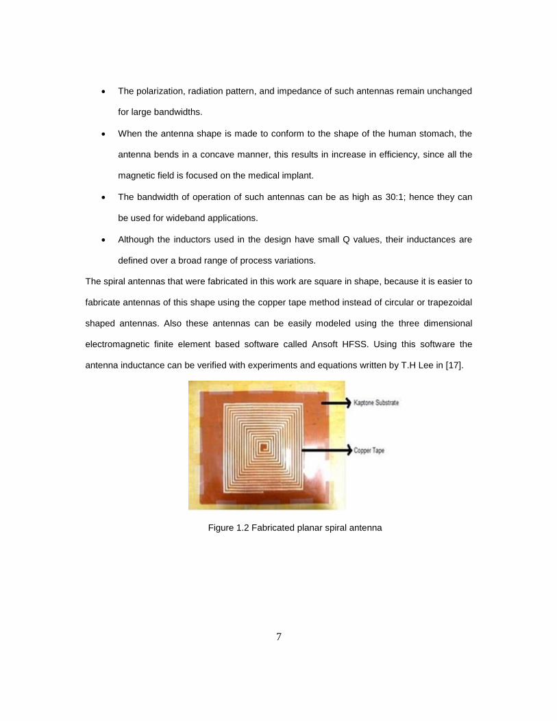
2.2.3 Cavity-backed slot antenna
The antennas discussed till now are those that are planar slot antennas. They can be
used in metallic backed objects such as aircraft body etc. It is desirable for the slot antenna to
be cavity backed, because this isolates the antenna from what is behind it, so that it can be
mounted on objects without worrying about retuning the antenna. These antennas come in two
types.
The first is a simple metallic backing separated from the antenna by some distance d.
This metallic backing will cause reflections of the radiated fields that enter the cavity, and these
often cancel the radiated fields that travel broadside to the plane of the antenna. If the depth d is
an integer multiple of half wavelength, the reflected field will tend to cancel the forward travelling
field of the spiral antenna, thus leading to poor radiation. Hence the wideband characteristics of
a metallic cavity backed slot antenna are less. An alternate method is to make use of absorbing
material to cavity back the spiral antenna. In this case, the reflected fields from the cavity will be
attenuated, so that there is no destructive interference, so the antenna will maintain its
wideband characteristics. This however tends to decrease the efficiency of the spiral antenna,
since roughly half the radiated power is radiated. However, this loss of efficiency is 3 dB, which
is often tolerable. An example of the cavity backed slot antenna is the cavity backed
Archimedean spiral antenna is shown below.
Figure 2.3 Cavity backed slot antenna [31]
13
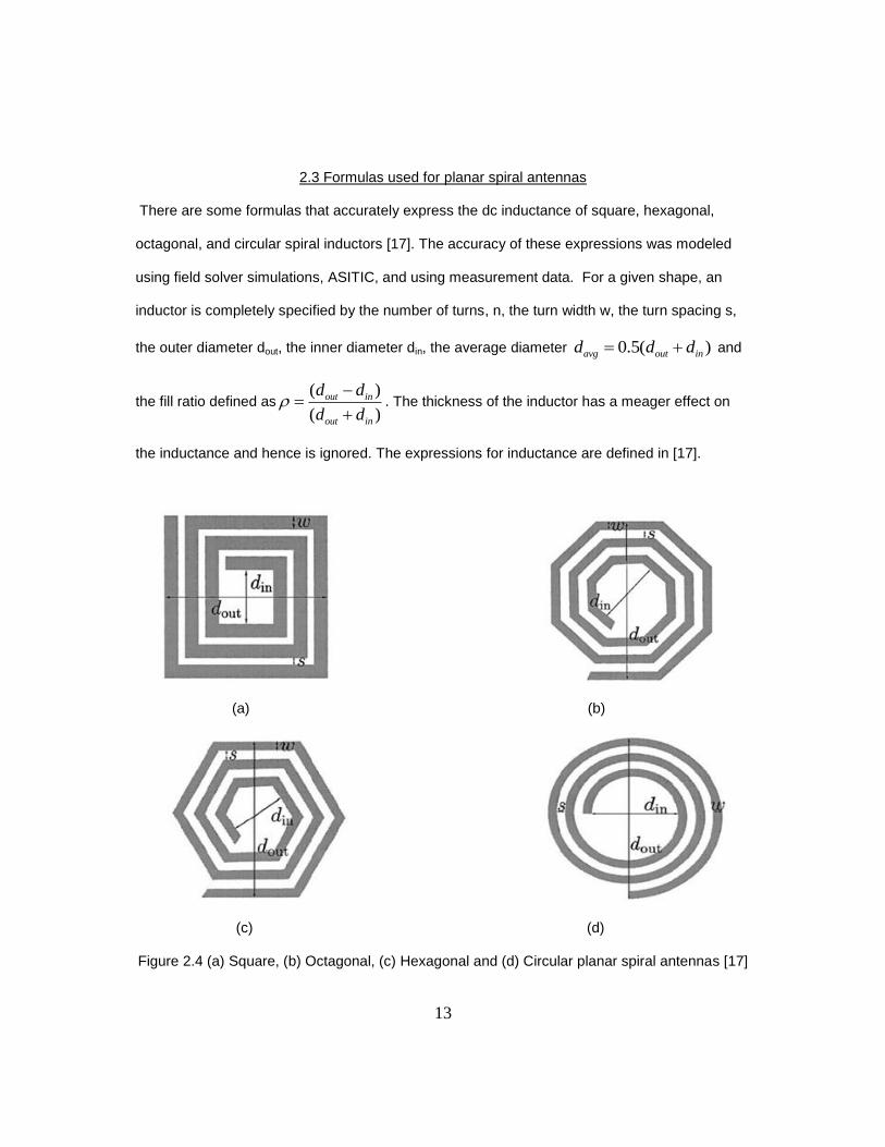
2.3 Formulas used for planar spiral antennas
There are some formulas that accurately express the dc inductance of square, hexagonal,
octagonal, and circular spiral inductors [17]. The accuracy of these expressions was modeled
using field solver simulations, ASITIC, and using measurement data. For a given shape, an
inductor is completely specified by the number of turns, n, the turn width w, the turn spacing s,
the outer diameter dout, the inner diameter din, the average diameter 0.5( )avg out ind d d and
the fill ratio defined as( )
( )
out in
out in
d d
d d
. The thickness of the inductor has a meager effect on
the inductance and hence is ignored. The expressions for inductance are defined in [17].
(a) (b)
(c) (d) Figure 2.4 (a) Square, (b) Octagonal, (c) Hexagonal and (d) Circular planar spiral antennas [17]

14
2.3.1 Modified wheeler formula
Wheeler presented several formulas for planar spiral inductors, which were intended for
discrete inductors. A simple modification of the wheeler formula can be used to obtain an
expression that is valid for planar spiral integrated inductors.
2
1
21
avg
mw o
n dL K
k
(2.3)
where is the fill ratio defined, previously. The coefficients 1K and 2K are layout dependent
and are shown in Table 2.1. The ratio, ,
is the fill ratio and represents how hollow the inductor
is. For a smaller ratio the inductor is hollow, and for a larger ratio the inductor is full. Two
inductors with the same average diameter but with different fill ratios will have different
inductances. The full inductor has a smaller inductance because its inner turns are closer to the
center of the spiral and hence would contribute less positive mutual inductance and more
negative mutual inductance
Table 2.1 Modified wheeler formula constants
2.3.2 Expression based on current sheet approximation
Another simple and accurate expression for planar spiral inductances can be obtained by
approximating the sides of the spirals by symmetrical current sheets of equivalent current
densities. For example, in case of a square, 4 identical current sheets are obtained. The current
sheets on opposite sides are parallel to each other, whereas the adjacent ones are orthogonal
to each other. Using symmetry and the fact that orthogonal current sheets have zero mutual
inductance, the computation of the inductance is now reduced to evaluating the self-inductance
of one sheet and the mutual inductance between the opposite current sheets. The self and

15
mutual inductances are evaluated using the concepts of geometric mean distance, arithmetic
mean distance, and the arithmetic mean square distance. The resulting expression [17] is
2
1 223 4(ln( ) )
2
avg
gmd
n d c cL c c
(2.4)
where ci are layout dependent given by the values in Table 2.2, s and w are the spacing
between the inductor turns and width of the inductor turns. Although the accuracy of the
expression reduces as the ratio, s/w, becomes large, it exhibits a maximum error of 8 % for s ≤
3w.
Table 2.2 Current sheet approximation formula constants
2.3.3 Data fitted monomial expression
This expression for inductance is obtained using a data fitting technique. The expression
is given by (2.5).
3 51 2 4
outmon avgL d d n s
(2.5)
where the coefficients β and αi are layout dependent and given in Table 2.3. The above
expression is monomial in the variables , , ,out avgd d n and s. The coefficients in (2.5) were
obtained using the following expressions 1x = log outd , 2 logx ,3 log avgx d , 4 logx n ,
5 logx s . Using logarithms, the expression (2.5) can be expressed as (2.6).
1 1 2 2 3 3 4 4 5 5log oy L x x x x x (2.6)
16
where logo . This is a linear plus constant model of y as a function of x, and is easily fit
by various data fitting and regression techniques. To develop the models, a simple least
squares fit is used. Also i is chosen to minimize (2.7).
( ) ( ) ( ) ( ) ( ) ( ) 2
1 1 2 2 3 3 4 4 5 5
1
( )N
k k k k k k
o
k
y x x x x x
(2.7)
where the sum is over a family of 19000 inductors.
Table 2.3 Data fitted monomial expression constants
The monomial expression (2.5) is useful since, like the other expressions (2.3), (2.4), it is
accurate and simple. It is used in optimal design of inductors
2.4 Planar spiral antenna fabrication techniques
There are different methods adopted in this research to fabricate the planar spiral
antennas. However, after making use of many methods, copper tape method was found to be
the easiest. The methods used are listed below.
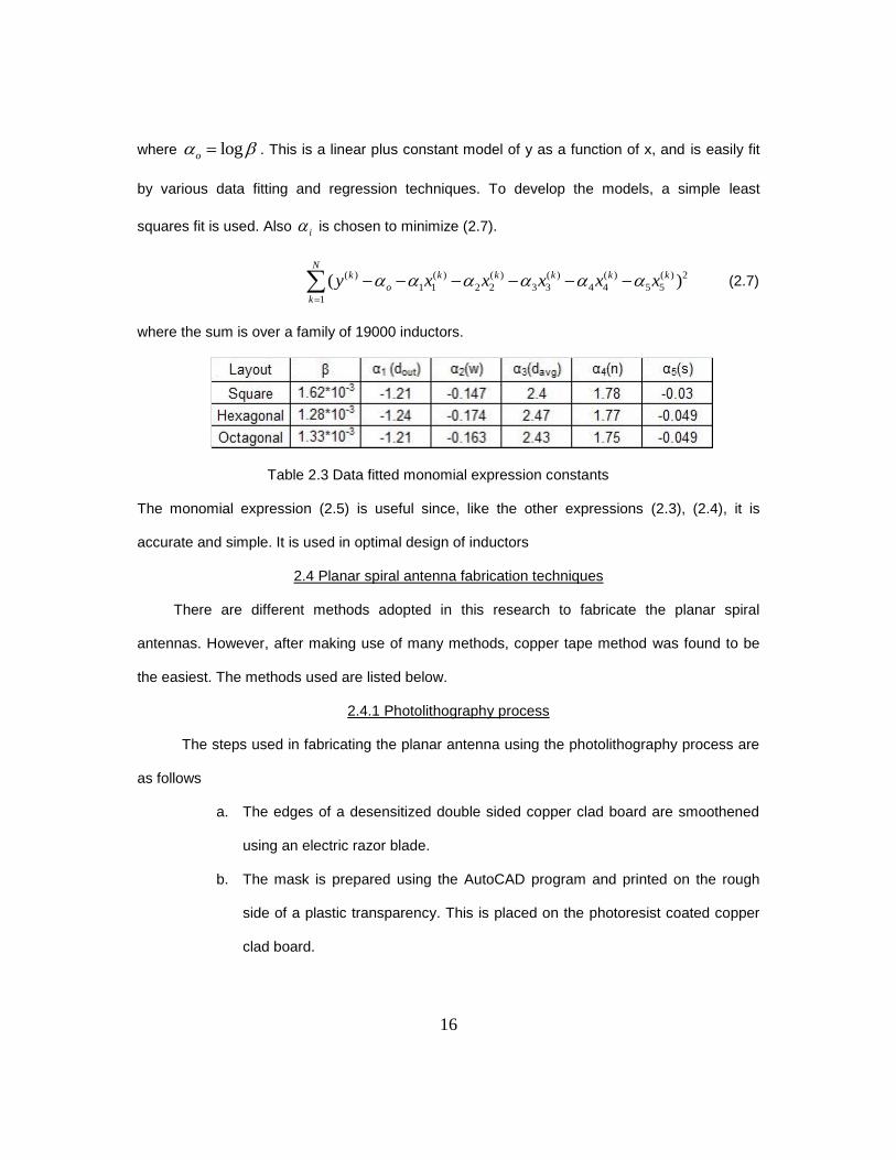
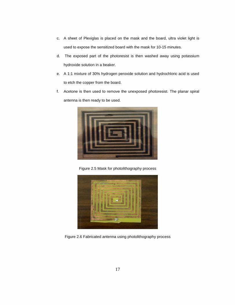
2.4.1 Photolithography process
The steps used in fabricating the planar antenna using the photolithography process are
as follows
a. The edges of a desensitized double sided copper clad board are smoothened
using an electric razor blade.
b. The mask is prepared using the AutoCAD program and printed on the rough
side of a plastic transparency. This is placed on the photoresist coated copper
clad board.
17
c. A sheet of Plexiglas is placed on the mask and the board, ultra violet light is
used to expose the sensitized board with the mask for 10-15 minutes.
d. The exposed part of the photoresist is then washed away using potassium
hydroxide solution in a beaker.
e. A 1:1 mixture of 30% hydrogen peroxide solution and hydrochloric acid is used
to etch the copper from the board.
f. Acetone is then used to remove the unexposed photoresist. The planar spiral
antenna is then ready to be used.
Figure 2.5 Mask for photolithography process
Figure 2.6 Fabricated antenna using photolithography process
18
2.4.1.1 Advantages of photolithography process
The process is less time consuming. It takes about half an hour to complete the antenna
fabrication process. The precision achieved is high as compared to other fabrication techniques
2.4.1.2 Disadvantages of photolithography process
The process is relatively expensive, because we are making use of different chemicals,
FR4 substrate. The process is very smelly, because of the release of hydrochloric acid vapors
during the etching process, which are corrosive in nature.
Since FR4 substrate can be used only once for antenna fabrication, different antenna
designs can only be executed using different substrates. This technique was discarded for cost
reasons.
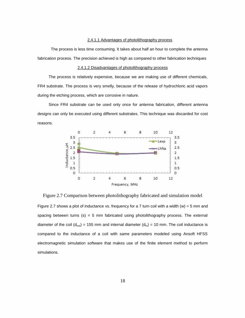
Figure 2.7 Comparison between photolithography fabricated and simulation model
Figure 2.7 shows a plot of inductance vs. frequency for a 7 turn coil with a width (w) = 5 mm and
spacing between turns (s) = 5 mm fabricated using photolithography process. The external
diameter of the coil (dout) = 155 mm and internal diameter (din) = 10 mm. The coil inductance is
compared to the inductance of a coil with same parameters modeled using Ansoft HFSS
electromagnetic simulation software that makes use of the finite element method to perform
simulations.

19
2.4.2 Copper tape method
Using this method, we can make use of a single substrate and easily change the design
of the antenna by peeling the copper tape and using another tape with a different design. The
steps followed to fabricate planar spiral antennas using this method are:
The substrate is first made stable by fixing it in a table using tape. The substrate used in
this research is kapton. Before making use of kapton substrate, wood was used for
preliminary experimental work.
Figure 2.8 Kapton taped on wooden platform
Copper tape is then taped on top of the substrate. Since the tape is of a particular
width, many strips of it are taped to cover the entire substrate. The tapes are attached
such that they partially overlap. This overlapping can cause discontinuities which can
later be prevented by using solder.
Figure 2.9 Copper strips stuck on kapton substrate

20
The mask of the planar spiral antenna made using AutoCAD software [18, 19] is then stuck on the copper tape.
Figure 2.10 Mask taped on copper layer
An impression is made on the mask along the spiral boundary using a pen knife and
then the mask is removed.
The copper tape is peeled from the substrate to obtain the planar spiral antenna.
The discontinuities in the coil are then soldered using tin-lead wire.
The antenna is then tested using an impedance analyzer. If the analyzer shows a
negative inductance, the antenna is checked for discontinuities and appropriate
connections are made until the analyzer reads positive inductance.

21
CHAPTER 3
ANSOFT HFSS SIMULATION
3.1 Finite element analysis
The finite element method (FEM) is a powerful numerical analysis technique which is
well-suited to and appropriate for solving a wide variety of electromagnetic applications
problems computationally [29]. Amongst the many methods used in computational
electromagnetics, its ability to manage problems with complex geometries, as well as its broad
applicability to static, quasi-static, wave and transient systems, and to problems containing
material regions that are nonlinear, inhomogeneous and anisotropic, all make the FEM one of
the most versatile and powerful computational analysis and simulation schemes available today.
Moreover, the solid theoretical foundations on which the FEM is based, as well as the rigorous
mathematical analysis concerning the existence, convergence, and the uniqueness of finite
element solutions that have been established, further justify its use in electromagnetics
research and design.
While FEM methods are presently used extensively for electromagnetics analysis and
design, the use of adaptive FEM methods has gained considerable attention in recent years
from numerical analysts for solving problems more efficiently than standard FEM methods
permit. The accuracy of a finite element solution is directly dependent on the number of free
parameters used to mathematically represent the problem, and how effectively those
parameters, or mathematical DOF(degrees of freedom), are distributed over the problem space.
Consequently, the most efficient distribution of DOF for a problem is that which provides a
sufficiently accurate solution for the lowest number of free parameters.
Currently, the only practical way to achieve this objective is by using adaptive solution
strategies which are capable of intelligently evolving and improving an efficient distribution of
22
DOF over the problem domain by establishing solution error distributions, and then adjusting or
adding DOF to the discretization to correct them. By increasing the number of DOF in the
vicinities of higher solution error only, it is possible to make the most significant improvement in
the global accuracy of the finite element solution, for the minimum additional computational
cost.
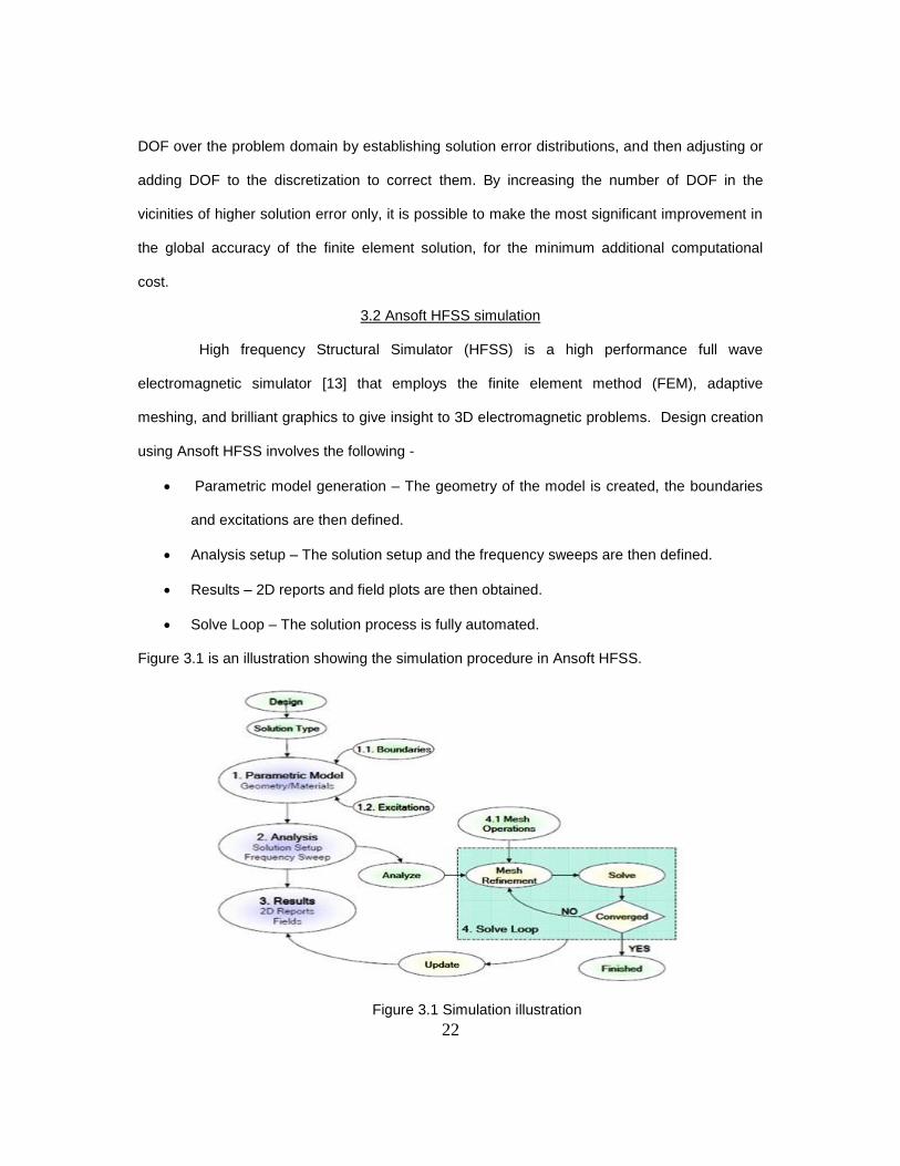
3.2 Ansoft HFSS simulation
High frequency Structural Simulator (HFSS) is a high performance full wave
electromagnetic simulator [13] that employs the finite element method (FEM), adaptive
meshing, and brilliant graphics to give insight to 3D electromagnetic problems. Design creation
using Ansoft HFSS involves the following -
Parametric model generation – The geometry of the model is created, the boundaries
and excitations are then defined.
Analysis setup – The solution setup and the frequency sweeps are then defined.
Results – 2D reports and field plots are then obtained.
Solve Loop – The solution process is fully automated.
Figure 3.1 is an illustration showing the simulation procedure in Ansoft HFSS.
Figure 3.1 Simulation illustration

23
3.3 Sample planar spiral antenna simulation setup
The following steps are involved in creating and simulating a planar spiral antenna -
To create a new project, we go to File and click on new project. From the project menu,
insert HFSS design option is selected.
Then solution type option from the HFSS menu item is selected and driven terminal
solution type is clicked.
From the 3D modeler menu item, unit’s option is selected and the appropriate units are
selected.
The 3D model of planar spiral antenna is then created using the HFSS graphical user
interface. Boundary conditions are applied and internal ports (lumped ports) are
assigned to the model. Care is taken that appropriate material properties are assigned
to different parts of the model.
From the HFSS menu option, analysis setup is selected and Add solution setup sub
option is then selected. The solution frequency, the maximum number of passes, and
the maximum error between each pass is then defined.
From the HFSS menu option, Analysis Setup is selected and Add sweep sub option is
then selected. The start frequency, stop frequency and the sweep type which is usually
interpolating is then selected.
The file is then saved and the validation check option from the HFSS menu option is
then selected to ensure whether there are any errors or not in the simulation setup.
The Analyze All option from the HFSS menu option is then selected. The simulation
then begins and ends when the solution converges.
From the HFSS menu option, the results option is selected and the create report sub
option is then selected.

24
The formulas for inductance and quality factor for the antenna are then inputted.
11
1Im( )
(2* * )
YL
pi freq & 11
11
1Im( )
1Re( )
YQ
Y
. These formulas [15, 28] are in the y axis of the
curve that is plotted with the x axis as frequency. The results are then exported in an
excel format and the values are obtained for frequency of interest.
A sample planar spiral inductor modeled using Ansoft HFSS is shown below –
(a) (b)
Figure 3.2 (a) Top view and (b) Side view of simulation model
3.4 Matching simulations with equations
Different designs of planar antennas were implemented in order to confirm the validity of
the equations in [17] with the simulation results. Since, it is clearly mentioned in [17] that the

25
inductance equations are only valid for dc frequencies; antennas with different designs were
simulated for different number of turns and for different dc (less than 800 kHz) frequencies.
Shown in Figure 3.5 is an antenna with a turn spacing and width of 8 mm, thickness of 0.1 mm
and an external diameter of 15 mm. An FR4 substrate of size 30 mm x 30 mm was used in
simulation.
Figure 3.3 HFSS spiral antenna model
Simulations were carried out for 500 KHz, 1 MHz, 1.3 MHz, 5 MHz and 10 MHz frequencies.
The values Lmw and Lgmd are inductance values obtained from formulas in [17]. The value Lhfss is
obtained from simulations performed in this research. As the frequency increases, it is observed
that the deviation of the three inductances increases from each other. This validates the fact,
that the inductance values Lmw and Lgmd are only valid for dc frequencies.
Figure 3.4 Simulation result for 500 kHz frequency

26
Figure 3.5 Simulation result for 5 MHz frequency
Shown in Figure 3.6 is another design of an antenna where the turn spacing and width are
equal to 0.2 mm and the thickness is equal to 0.1 mm. The external diameter of the antenna is
50 mm. The substrate size is 100 mm x 100 mm and thickness is 1.5 mm. The graphs shown in
Figure 3.8 and Figure 3.9 also show the deviation of the three inductances with the increase in
frequency.
Figure 3.6 Simulation result for 500 kHz frequency

27
Figure 3.7 Simulation result for 5 MHz frequency
3.5 Matching simulations with publications
In order to ensure that the simulations performed using Ansoft HFSS are correct,
Several IEEE papers [25, 26, 27] were implemented and the HFSS results obtained from
simulations carried out in research work were matched with the HFSS results obtained from the
IEEE papers. Figure 3.10 shows the results obtained from [24].
Figure 3.8 Publication [24] Vs. Simulation result
Here the values Lmy Simulation and Lpaper are the inductances of the model implemented in this
research and the author. There is a small variation in the results between the simulation by
28
these authors and this research simulation, this can be explained by the different software
versions used and the size of the radiation boundaries.
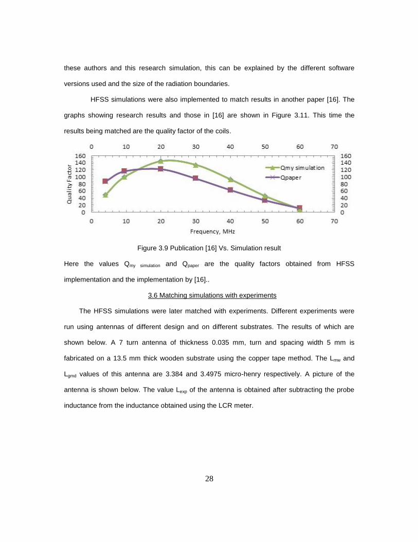
HFSS simulations were also implemented to match results in another paper [16]. The
graphs showing research results and those in [16] are shown in Figure 3.11. This time the
results being matched are the quality factor of the coils.
Figure 3.9 Publication [16] Vs. Simulation result
Here the values Qmy simulation and Qpaper are the quality factors obtained from HFSS
implementation and the implementation by [16]..
3.6 Matching simulations with experiments
The HFSS simulations were later matched with experiments. Different experiments were
run using antennas of different design and on different substrates. The results of which are
shown below. A 7 turn antenna of thickness 0.035 mm, turn and spacing width 5 mm is
fabricated on a 13.5 mm thick wooden substrate using the copper tape method. The Lmw and
Lgmd values of this antenna are 3.384 and 3.4975 micro-henry respectively. A picture of the
antenna is shown below. The value Lexp of the antenna is obtained after subtracting the probe
inductance from the inductance obtained using the LCR meter.
29
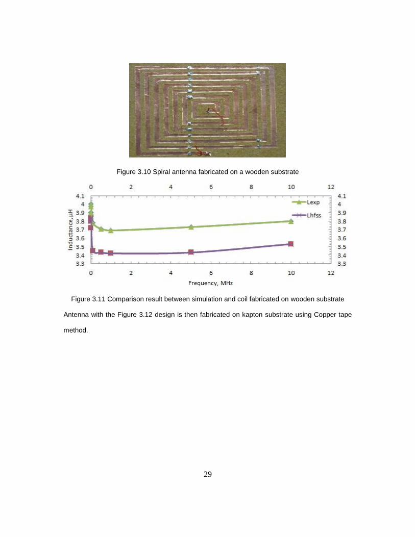
Figure 3.10 Spiral antenna fabricated on a wooden substrate
Figure 3.11 Comparison result between simulation and coil fabricated on wooden substrate
Antenna with the Figure 3.12 design is then fabricated on kapton substrate using Copper tape
method.

30
Figure 3.12 Spiral antenna fabricated on kapton substrate
Figure 3.13 Comparison result between simulation and coil fabricated on kapton substrate
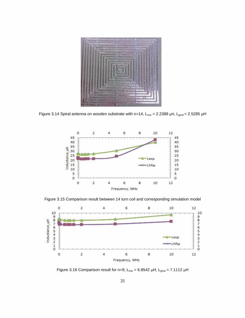
A 14 turn planar spiral antenna is then fabricated on a wooden substrate of thickness
13.5 mm. The turn and spacing width of the antenna is 5 mm and the thickness of the copper
coil is 0.035 mm. The fabrication is performed using copper tape method. HFSS simulations
and measurements are then performed for different turns and the results are compared.
31
Figure 3.14 Spiral antenna on wooden substrate with n=14, Lmw = 2.2388 µH, Lgmd = 2.5285 µH
Figure 3.15 Comparison result between 14 turn coil and corresponding simulation model
Figure 3.16 Comparison result for n=9, Lmw = 6.8542 µH, Lgmd = 7.1112 µH

32
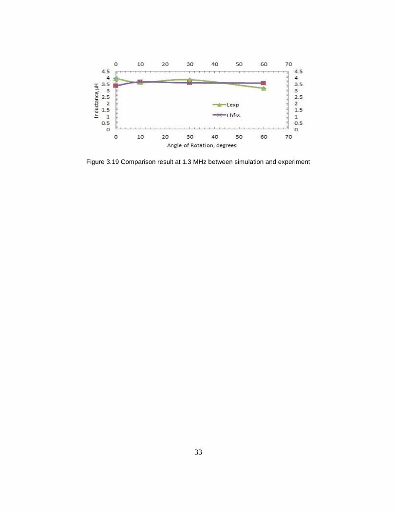
3.7 Matching simulations with bent antenna
The coil antenna is fabricated on a flexible substrate in order to provide comfort to the patient
who is wearing it. Since a bent coil is used, simulation has to be also performed in HFSS for
bent coils. Since HFSS does not provide a method to bend the coil, the coil model has to be
exported to a format that can be used by a different program that allows for a bent substrate to
bend it. AutoDesSys Inc. provides software called Bonzai 3d that can be used to bend the coil
along any plane and to any degree. After bending the coil, the bent coil model can be exported
to a format that can be imported into HFSS for performing simulations.
After modeling the coil in HFSS, the model can be exported in .sat format. The (.sat)
file can later be imported into Bonzai 3d software [20].The software has a bend function that can
be used to bend the coil antenna to any degree and along XY, YZ or XZ axis. In this case the
model was bent along XZ axis. The bent coil model is then exported in .sat (standard ACIS text)
format. The file is then imported into HFSS and after applying boundary conditions, excitations,
the simulation is then started. A sample 7 turn coil model is simulated after being bent and the
results are compared to experimental results.
Figure 3.17 Top view of bent antenna model Figure 3.18 Side view of bent antenna model
33
Figure 3.19 Comparison result at 1.3 MHz between simulation and experiment
34
CHAPTER 4
FLEXIBLE ANTENNA EXPERIMENTS
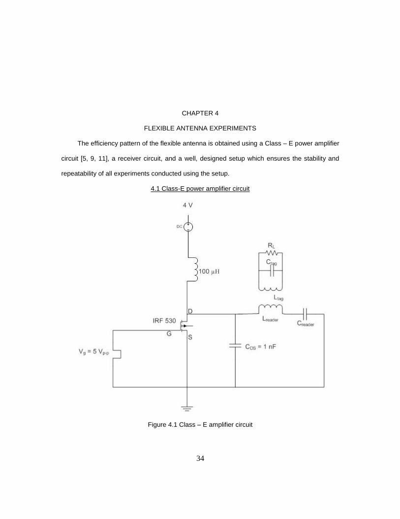
The efficiency pattern of the flexible antenna is obtained using a Class – E power amplifier
circuit [5, 9, 11], a receiver circuit, and a well, designed setup which ensures the stability and
repeatability of all experiments conducted using the setup.
4.1 Class-E power amplifier circuit
Figure 4.1 Class – E amplifier circuit

35
Class – E amplifiers can operate with power losses smaller by a factor of 2.3 [11] compared
with conventional Class – B or Class - C amplifiers making use of the same transistor at the
same frequency and output power. Class – E power amplifiers also have a very high efficiency
compared to other conventional amplifiers. Hence, it is used in this experimental work described
in this thesis. Also the MOSFET used is IRF 530 (enhancement type N channel MOSFET),
because it has a low threshold voltage and has a higher efficiency as compared to IRF 510
transistor.
The amplifier operates as follows. The 100 µH inductor connected at the drain acts as a
constant current source. When the switch closes, LReader supplies current through the switch and
no current flows through CDS. When the switch opens, the inductor supplies current through CDS
and no current flows through the switch thereby building a voltage across the switch. The
amplifier operation is such that the voltage and current at the switch have a phase difference of
90 degrees at all times. This results in very low power losses and high efficiency of the
amplifier. There is a particular value of CReader and CTag at which the amplifier resonates at 1.3
MHz frequency and the efficiency of power transfer between the LReader and LTag through the
resonant magnetic coupling phenomenon, is maximum. Care is always taken that resonance is
achieved before obtaining the efficiency patterns for any of the antenna characterization
configurations so that stability and hence repeatability of the experiments is ensured.
The efficiency of power transfer between the two coils is calculated based on equations (4.1) –
(4.3).
i DD DDP V I (4.1)
where iP is the input power and the dc voltage DDV is fixed at 4 V.
2 2
500o
Load
V VP
R (4.2)

36
where V is the voltage across the load resistor and oP is the output power delivered to the
load.
The efficiency of power transfer is then calculated using (4.3).
In % = 100%O
i
P
P . (4.3)
4.2 Introduction to experiments
Four different experiments are performed to characterize the flexible antenna.
Antenna misalignment – The tag antenna is fixed and the reader antenna is rotated
along a particular curvature. The angle at which both the reader antenna and tag
antenna are center aligned is considered 0 degrees. The clockwise rotation of the
reader antenna is considered positive rotation and the anticlockwise rotation of the
reader antenna is considered negative rotation. A graph is obtained with the reader
antenna angular rotation plotted along the x axis and the efficiency values at the
corresponding reader antenna positions plotted along the y axis. The experiment is
repeated for all 3 different curvatures of the reader antenna and at tag antenna
distances of 4 cm, 6 cm and 8 cm from the reader antenna.
Antenna pattern - The reader antenna is fixed and the tag antenna is rotated along its
axis. The angle at which both the reader antenna and tag antenna are center aligned is
considered 0 degrees. The clockwise rotation of the tag antenna is considered positive
rotation and the anticlockwise rotation of the tag antenna is considered negative
rotation. A graph is obtained with the tag antenna angular rotation plotted along the x
axis and the efficiency values at the corresponding tag antenna positions plotted along
the y axis. The experiment is repeated for all 3 different curvatures of the reader
antenna and at tag antenna distances of 4 cm, 6 cm and 8 cm from the reader antenna.
Cross section pattern – The reader antenna is fixed and the tag antenna is moved
upwards and downwards with the distance between the two antennas fixed. The

37
position at which both the reader antenna and tag antenna are center aligned is
considered the origin. The upward movement of the tag antenna is considered negative
movement from the origin and the downward movement of it is considered positive
movement from the origin. A graph is plotted with tag antenna movement from the
origin, along the x axis and the efficiency values at the corresponding tag antenna
positions along the y axis. The experiment is repeated for all 3 different curvatures of
the reader antenna and at tag antenna distances of 4 cm, 6 cm and 8 cm from the
reader antenna.
3D pattern – To perform the experiment two acrylic plates are used. The reader
antenna is fixed in the reader plate using tape. A tag antenna plate is made by making
a 26 cm x 26 cm square pattern of holes spaced 1 cm apart. The tag antenna is moved
along these holes at distances of 2 cm apart and the efficiency of power transfer is
measured. At the end the efficiency pattern is obtained for 13 cm x 13 cm square
matrix. The reader antenna is fixed and the tag antenna plate is moved at distances of
4 cm, 6 cm and 8 cm from the reader antenna plate and the efficiency pattern is
obtained. For references and efficiency pattern plotting, two axis – the x axis and y axis
are used. The vertical upward and downward movement of the tag antenna in the tag
antenna plate is considered negative and positive movement of the tag antenna along
the x axis. The horizontal east and west movement of the tag antenna is considered
positive and negative movement of the tag antenna along the y axis.
4.3 Antenna characterization setup requirements
In order to obtain an accurate characterization [12] of an antenna, the following steps need
to be taken.
The system needs to be very stable. This can be realized by building a system that requires
the least human intervention. The setup should be such that, the reliability of the measurements
should be maintained. Hence the experiments performed should be repeatable. The setup

38
should be small and easy to handle to promote ease of experiments with minimum errors. This
would require the setup to be reconfigurable. The setup should be such that, a large number of
readings from the setup can be taken in a short interval of time. Unnecessary hardware
components should be removed to reduce hardware costs. A better measurement sensitivity
capability should be maintained in order to obtain experimental accuracy.
4.4 Experimental setup design
In order to realize such a system, where the above conditions are met, a design was made
and was accurately fabricated using a CNC machine. The design of the setup for one groove is
shown in Figure 4.2.
Figure 4.2 Top view of entire setup with a schematic of rotation angle of reader antenna
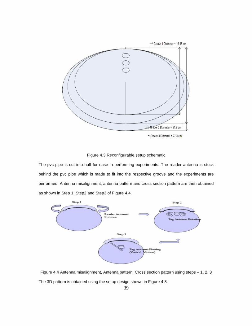
In order to make the setup reconfigurable and, as per the dimensions mentioned in Figure 4.3,
three grooves were made of diameters equal to the diameters of 3 pvc pipes. Three holes were
made at distances 4 cm, 6 cm and 8 cm from the 0 degree position (origin) mentioned in Figure
4.2. These holes were made to fit the acrylic stick into which tag antenna would be fixed using
tooth pick and tape. A schematic of the three grooves and holes is shown in Figure 4.3.
39
Figure 4.3 Reconfigurable setup schematic
The pvc pipe is cut into half for ease in performing experiments. The reader antenna is stuck
behind the pvc pipe which is made to fit into the respective groove and the experiments are
performed. Antenna misalignment, antenna pattern and cross section pattern are then obtained
as shown in Step 1, Step2 and Step3 of Figure 4.4.
Figure 4.4 Antenna misalignment, Antenna pattern, Cross section pattern using steps – 1, 2, 3
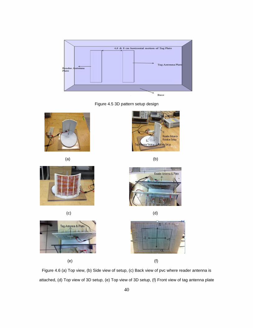
The 3D pattern is obtained using the setup design shown in Figure 4.8.
40
Figure 4.5 3D pattern setup design
(a) (b)
(c) (d)
(e) (f)
Figure 4.6 (a) Top view, (b) Side view of setup, (c) Back view of pvc where reader antenna is
attached, (d) Top view of 3D setup, (e) Top view of 3D setup, (f) Front view of tag antenna plate

41
4.5 Experiment parameters
After achieving a good experimental set up, experiments were conducted and the
parameters used are discussed. Experiments were conducted using three curvatures C1 of radii
= 8.4 cm, C2 of radii = 11 cm and C3 of radii = 14 cm. As discussed before, three half sections
of pvc pipes were used to emulate the bend. Based on the radii C1 had the highest bend, C2
had the second highest bend, and C3 had the least bend. Antennas with two different designs
were used in the experiments. Since with bending of the coil, antenna inductance reduces and
the transmitter circuit had to be retuned for each bend [7, 8]. The receiver circuit is changed
only once when tuning the antenna for the first time when it is straight. There after only the
transmitter circuit is retuned. Also the two antennas are abbreviated as A1 and A2. The
component parameters are mentioned in Table 4.1.

42
Table 4.1 Experiment parameters
4.6 Antenna characterization results
Legends shown in the graphs of Figure 4.7 – Figure 4.26 and Figure 4.30 – Figure 4.49,
consists of 4 parts separated by commas. The first part is the antenna used – A1 or A2. The
second part is the curvature used – C1, C2, C3 or St (straight). The third part is the distance
between the reader coil and tag coil. The fourth part is the experiment conducted – A.M
(Antenna Misalignment), A.P (Antenna Pattern), C.P (Cross-section Pattern) and 3D.P (3D
Pattern).
43
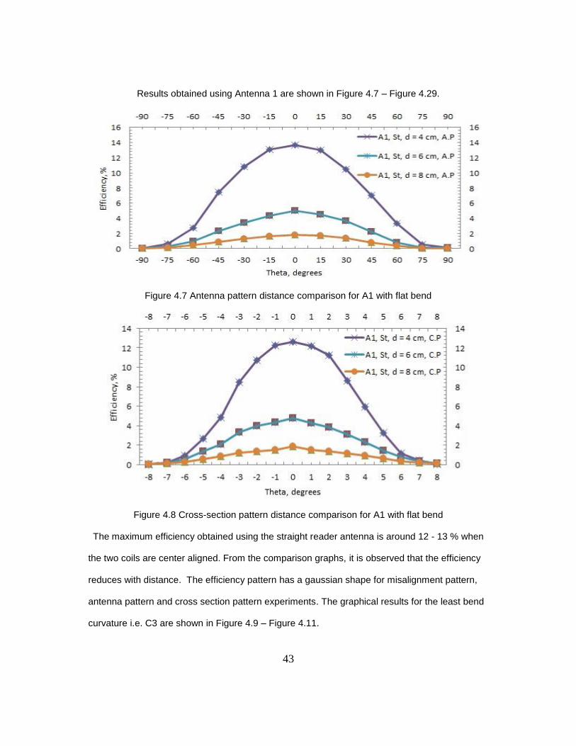
Results obtained using Antenna 1 are shown in Figure 4.7 – Figure 4.29.
Figure 4.7 Antenna pattern distance comparison for A1 with flat bend
Figure 4.8 Cross-section pattern distance comparison for A1 with flat bend
The maximum efficiency obtained using the straight reader antenna is around 12 - 13 % when
the two coils are center aligned. From the comparison graphs, it is observed that the efficiency
reduces with distance. The efficiency pattern has a gaussian shape for misalignment pattern,
antenna pattern and cross section pattern experiments. The graphical results for the least bend
curvature i.e. C3 are shown in Figure 4.9 – Figure 4.11.

44
Figure 4.9 Antenna misalignment distance comparison for A1 with C3 bend
Figure 4.10 Antenna pattern distance comparison for A1 with C3 bend
45
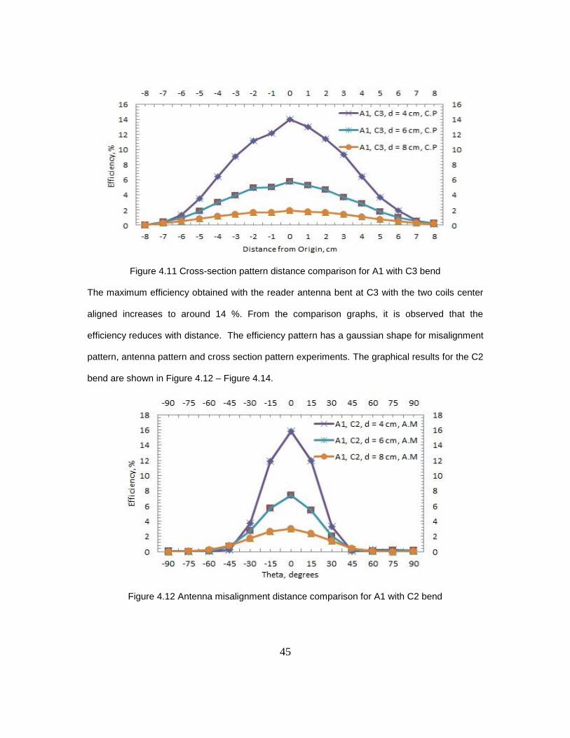
Figure 4.11 Cross-section pattern distance comparison for A1 with C3 bend
The maximum efficiency obtained with the reader antenna bent at C3 with the two coils center
aligned increases to around 14 %. From the comparison graphs, it is observed that the
efficiency reduces with distance. The efficiency pattern has a gaussian shape for misalignment
pattern, antenna pattern and cross section pattern experiments. The graphical results for the C2
bend are shown in Figure 4.12 – Figure 4.14.
Figure 4.12 Antenna misalignment distance comparison for A1 with C2 bend

46
Figure 4.13 Antenna pattern distance comparison for A1 with C2 bend
Figure 4.14 Cross-section pattern distance comparison for A1 with C2 bend
The maximum efficiency obtained with the reader antenna bent at C2 with the two coils center
aligned increases to around 16 % - 17 %. From the comparison graphs, it is observed that the
efficiency reduces with distance which can be explained from inverse square law. The
efficiency pattern has a gaussian shape for misalignment pattern, antenna pattern and cross
47
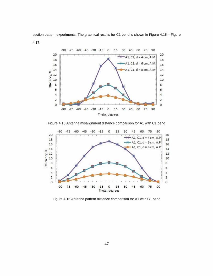
section pattern experiments. The graphical results for C1 bend is shown in Figure 4.15 – Figure
4.17.
Figure 4.15 Antenna misalignment distance comparison for A1 with C1 bend
Figure 4.16 Antenna pattern distance comparison for A1 with C1 bend
48
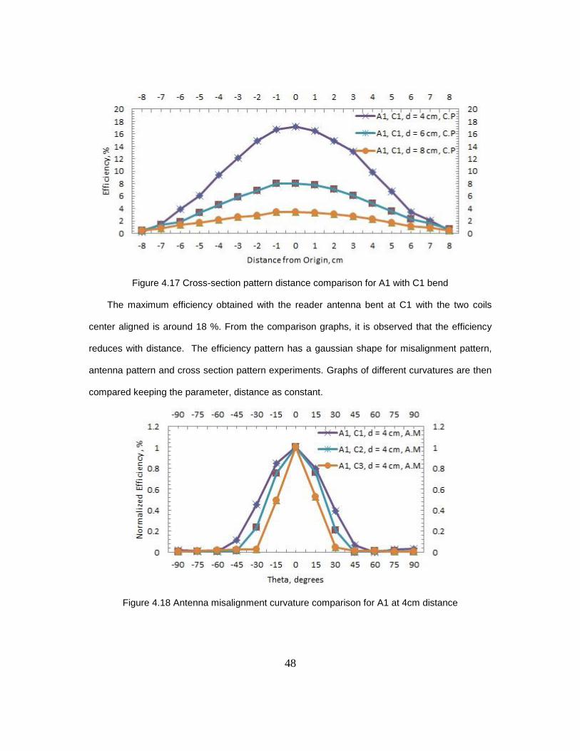
Figure 4.17 Cross-section pattern distance comparison for A1 with C1 bend
The maximum efficiency obtained with the reader antenna bent at C1 with the two coils
center aligned is around 18 %. From the comparison graphs, it is observed that the efficiency
reduces with distance. The efficiency pattern has a gaussian shape for misalignment pattern,
antenna pattern and cross section pattern experiments. Graphs of different curvatures are then
compared keeping the parameter, distance as constant.
Figure 4.18 Antenna misalignment curvature comparison for A1 at 4cm distance
49
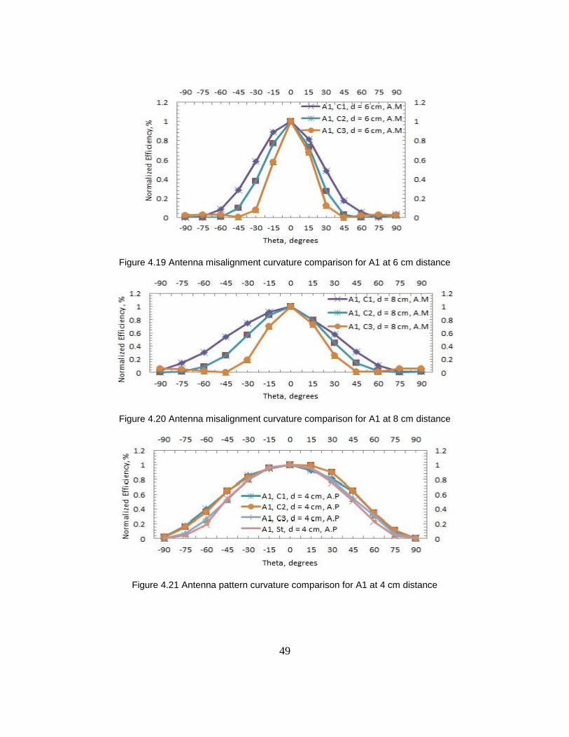
Figure 4.19 Antenna misalignment curvature comparison for A1 at 6 cm distance
Figure 4.20 Antenna misalignment curvature comparison for A1 at 8 cm distance
Figure 4.21 Antenna pattern curvature comparison for A1 at 4 cm distance
50
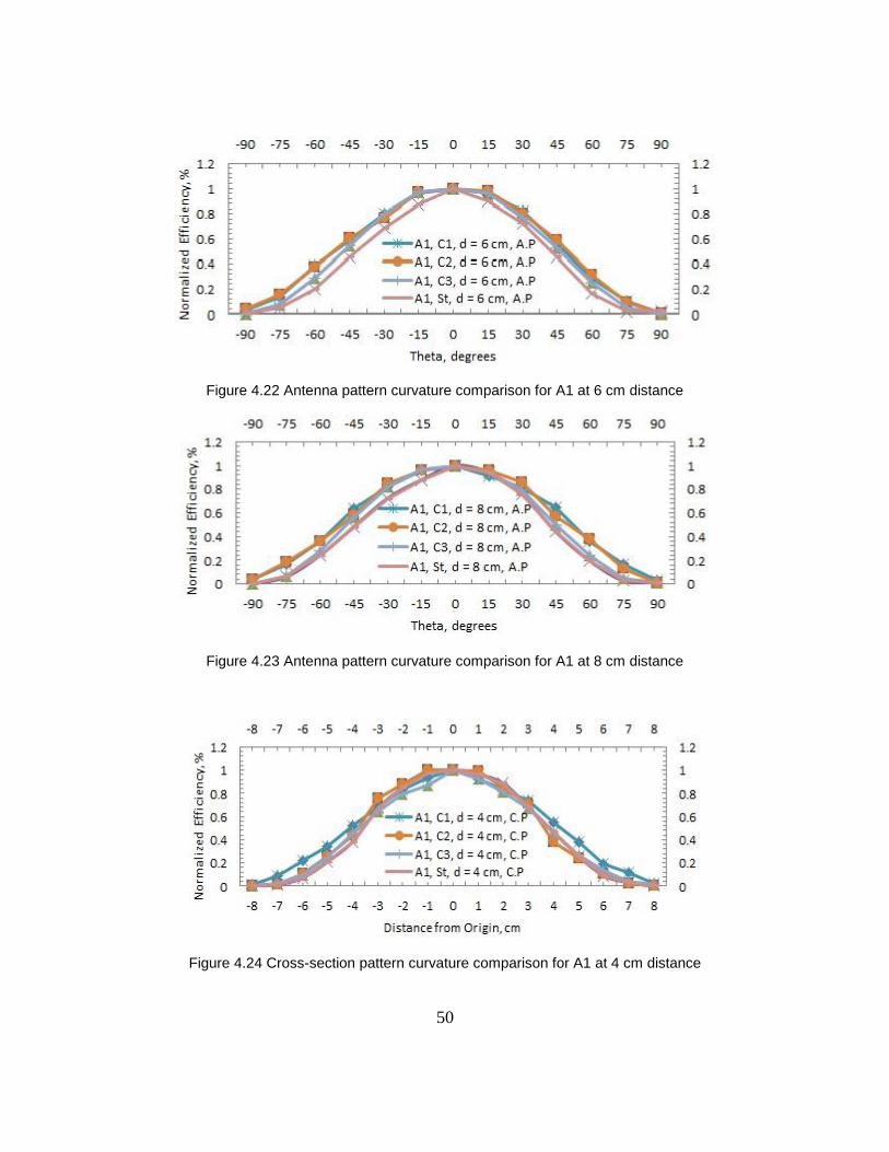
Figure 4.22 Antenna pattern curvature comparison for A1 at 6 cm distance
Figure 4.23 Antenna pattern curvature comparison for A1 at 8 cm distance
Figure 4.24 Cross-section pattern curvature comparison for A1 at 4 cm distance

51
Figure 4.25 Cross-section pattern curvature comparison for A1 at 6 cm distance
Figure 4.26 Cross-section pattern curvature comparison for A1 at 8 cm distance
From the curvature comparison results shown in Figure 4.18 – Figure 4.26, it is observed that
the bandwidth increases with increase in bend and increase in distance. 3D plotting
experiments were conducted later to obtain a plot at distances of 4 cm, 6 cm and 8 cm. 169
data points were collected at each distance.
52
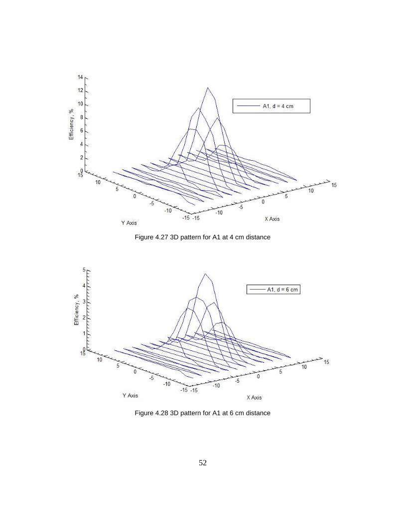
Figure 4.27 3D pattern for A1 at 4 cm distance
Figure 4.28 3D pattern for A1 at 6 cm distance
53
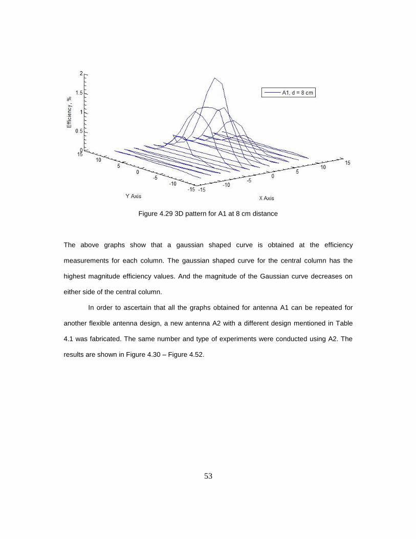
Figure 4.29 3D pattern for A1 at 8 cm distance
The above graphs show that a gaussian shaped curve is obtained at the efficiency
measurements for each column. The gaussian shaped curve for the central column has the
highest magnitude efficiency values. And the magnitude of the Gaussian curve decreases on
either side of the central column.
In order to ascertain that all the graphs obtained for antenna A1 can be repeated for
another flexible antenna design, a new antenna A2 with a different design mentioned in Table
4.1 was fabricated. The same number and type of experiments were conducted using A2. The
results are shown in Figure 4.30 – Figure 4.52.
54
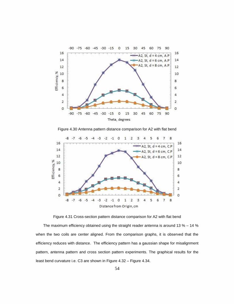
Figure 4.30 Antenna pattern distance comparison for A2 with flat bend
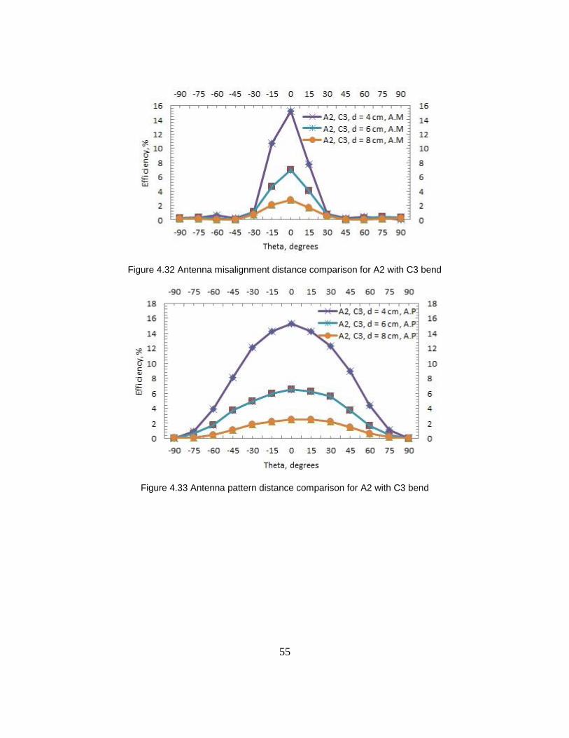
Figure 4.31 Cross-section pattern distance comparison for A2 with flat bend
The maximum efficiency obtained using the straight reader antenna is around 13 % – 14 %
when the two coils are center aligned. From the comparison graphs, it is observed that the
efficiency reduces with distance. The efficiency pattern has a gaussian shape for misalignment
pattern, antenna pattern and cross section pattern experiments. The graphical results for the
least bend curvature i.e. C3 are shown in Figure 4.32 – Figure 4.34.
55
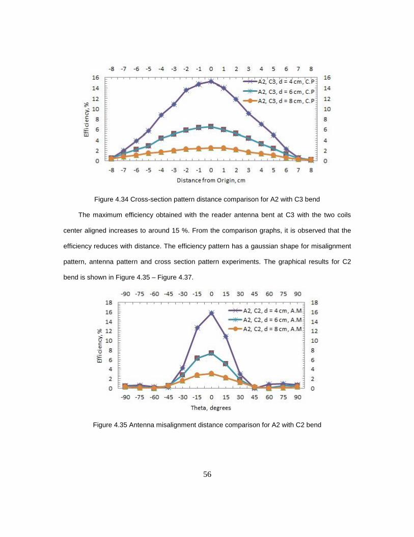
Figure 4.32 Antenna misalignment distance comparison for A2 with C3 bend
Figure 4.33 Antenna pattern distance comparison for A2 with C3 bend
56
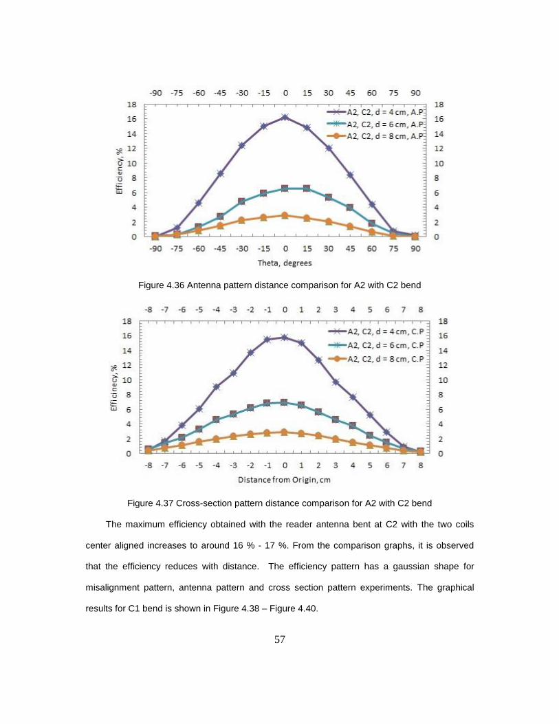
Figure 4.34 Cross-section pattern distance comparison for A2 with C3 bend
The maximum efficiency obtained with the reader antenna bent at C3 with the two coils
center aligned increases to around 15 %. From the comparison graphs, it is observed that the
efficiency reduces with distance. The efficiency pattern has a gaussian shape for misalignment
pattern, antenna pattern and cross section pattern experiments. The graphical results for C2
bend is shown in Figure 4.35 – Figure 4.37.
Figure 4.35 Antenna misalignment distance comparison for A2 with C2 bend
57
Figure 4.36 Antenna pattern distance comparison for A2 with C2 bend
Figure 4.37 Cross-section pattern distance comparison for A2 with C2 bend
The maximum efficiency obtained with the reader antenna bent at C2 with the two coils
center aligned increases to around 16 % - 17 %. From the comparison graphs, it is observed
that the efficiency reduces with distance. The efficiency pattern has a gaussian shape for
misalignment pattern, antenna pattern and cross section pattern experiments. The graphical
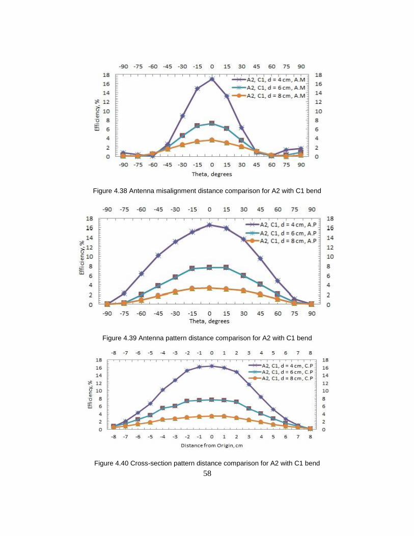
results for C1 bend is shown in Figure 4.38 – Figure 4.40.
58
Figure 4.38 Antenna misalignment distance comparison for A2 with C1 bend
Figure 4.39 Antenna pattern distance comparison for A2 with C1 bend
Figure 4.40 Cross-section pattern distance comparison for A2 with C1 bend

59
The maximum efficiency obtained with the reader antenna bent at C1 with the two coils
center aligned increases to around 18%. From the comparison graphs, it is observed that the
efficiency reduces with distance which can be explained from inverse square law. The
efficiency pattern has a gaussian shape for misalignment pattern, antenna pattern and cross
section pattern experiments. Graphs of different curvatures are then compared keeping the
parameter, distance as constant.
Figure 4.41 Antenna misalignment curvature comparison for A2 at 4 cm distance
Figure 4.42 Antenna misalignment curvature comparison for A2 at 6 cm distance
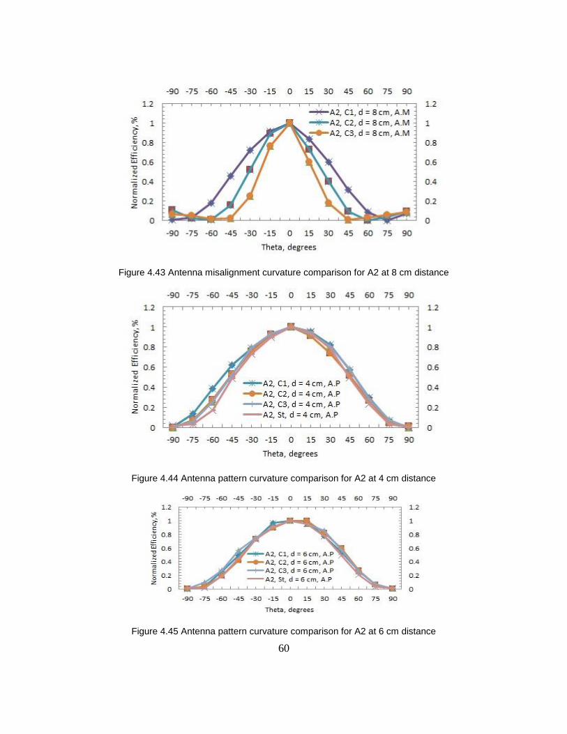
60
Figure 4.43 Antenna misalignment curvature comparison for A2 at 8 cm distance
Figure 4.44 Antenna pattern curvature comparison for A2 at 4 cm distance
Figure 4.45 Antenna pattern curvature comparison for A2 at 6 cm distance

61
Figure 4.46 Antenna pattern curvature comparison for A2 at 8 cm distance
Figure 4.47 Cross-section pattern curvature comparison for A2 at 4 cm distance
Figure 4.48 Cross-section pattern curvature comparison for A2 at 6 cm distance

62
Figure 4.49 Cross-section pattern curvature comparison for A2 at 8 cm distance
From the curvature comparison results shown in Figure 4.41 – Figure 4.49, it is observed
that the bandwidth increases with increase in bend and increase in distance. 3D plotting
experiments were conducted later to obtain a plot at distances of 4 cm, 6 cm and 8 cm. 169
data points were collected at each distance.
Figure 4.50 3D pattern for A2 at 4 cm distance

63
Figure 4.51 3D pattern for A2 at 6 cm distance
Figure 4.52 3D pattern for A2 at 8 cm distance

64
The above graphs show that a Gaussian curve is obtained at the efficiency measurements for
each column. The Gaussian curve for the central column has the highest magnitude efficiency
values. And the magnitude of the Gaussian curve decreases on either side of the central
column.
4.7 Explanation of the results
Faraday, showed that the magnitude of electromagnetic force generated in the coil is
proportional to the rate of change of magnetic flux passing through all the turns of the coil. With
the displacement of either antenna that causes misalignment between the centers of the two
coils, the passage of magnetic flux through all the turns of the Tag antenna reduces, thus
causing the reduction in emf generated at the tag coil, hence the reduction in efficiency. This
phenomenon is verified by the graphs obtained.
It was found from experiments that by using a straight coil, the efficiency obtained is
around 12% which is less than other curvatures used. By increasing the distance between
reader antenna and the tag antenna the efficiency decreases, because of the inverse square
law. From the graphs, it is observed that the efficiency of power transfer decreases on either
side of the zero position of the reader antenna. The curve is Gaussian shaped, and since the
power transferred between the two antennas is due to change in magnetic flux linking the two
coils, the intensity of magnetic field distribution on either side of the zero position is gaussian.
Gaussian distribution of magnetic field intensity is observed, when both the reader and tag coils
are rotated, keeping either antenna static when the other is rotated. Also the cross section
pattern follows a gaussian distribution, indicating that the magnetic flux density is strongest at
the center of the antenna and reduces in a gaussian manner, as the tag antenna is moved away
from the center. From, the comparison graphs shown above, a summarized picture of the
magnetic field distribution is obtained. The 3D pattern gives a better picture of the magnetic field
distribution between the reader and tag antennas. From the gaussian shaped curves obtained
by moving the tag across each row of the tag plate, it is understood how the magnetic field

65
varies in the three dimensional region between the reader antenna and tag antenna. The
gaussian shape of the curves can be explained by the below formulas [31].
2
( , )( , )
4t
GW P
r
(4.4)
where W is the power density of the incident radiation from the reader antenna. and
indicate the direction dependence of the parameters. G is the gain of the reader antenna which
is dependent on the radiation efficiency, antenna gain and mismatch losses between reader
antenna and transmitter circuit. tP is the power the reader antenna would deliver to a matched
load. r is the distance between the reader and tag antennas.
( , )rP A W (4.5)
where rP is the power delivered to the tag antenna, A is the effective aperture of the tag
antenna which is the effective area of the tag antenna that directly intercepts the power
transmitted by the reader antenna.
24
r
t
P GA
P r (4.6)
(4.6) is obtained from (4.4) and (4.5) and is the efficiency of power received at the tag antenna.
The efficiency depends on the effective aperture of tag antenna, gain of the reader antenna and
the distance between the tag and reader antennas. The gain of the reader antenna is constant
since the source is constant. Hence the curves obtained in Figure 4.7 – Figure 4.52 are
dependent on the effective aperture of the tag antenna and the distance between the tag and
reader antennas.
By increasing the bend of the coil by using pvc pipes, an efficiency of around 14%, 16%
and 18% is obtained between center-aligned reader and tag antennas. Thus there is
approximately, an increase of 2% in the power transfer efficiency with the increase in the
bending radius of the coil by 4 cm. This hints that the magnetic flux at the center of the two coils

66
increases due to contribution from the sides of the reader antenna. And with the increase in
bend, the contribution made from either side of the reader antenna center, increases.

67
CHAPTER 5
CONCLUSION
Simulation model was established using Ansoft HFSS program. To ensure simulation
results obtained from Ansoft HFSS software are accurate a spiral antenna simulation model had
to be established. Planar spiral antenna formulae referred from [17] were used. Since the
results obtained from these formulae are only valid at dc frequencies, different spiral antenna
designs were used and simulated to match the results obtained from the formulae. The results
matched. Two IEEE papers [16, 24] were used to ascertain whether the model is correct.
Inductance and quality factor results obtained from these two papers also matched with the
appropriate models made in HFSS.
The experimental results validated simulation model. The next step was to ascertain
whether the experimentally fabricated inductor results matched the HFSS simulation results.
Two different substrates, wood and kapton, were used and 35 experiments were conducted
using inductors of different design. The simulation results matched the HFSS model in all the
experiments.
Power transfer efficiency and radiation pattern were experimentally tested. A total of
125 experiments were conducted using a stable well designed setup. Experiments were
conducted using two different reader antennae, three different bending angles of reader
antenna at three different distances. All results obtained were compared with results obtained
from a straight reader antenna. 3D radiation pattern experiments were conducted and the
results obtained, establish the radiation pattern in the space between the reader and tag
antenna. Using four different experiments the power transfer efficiency was obtained and the
radiation pattern was thus established.

68
Flat and curve antenna with three different curvatures were tested. Three different
curvatures C1 of 8.4 cm bend, C2 of 11.4 cm bend and C3 of 14 cm bend were used in the
characterization experiments and the reader antenna was bent along these curvatures and
tested. The antenna pattern comparison results show that the pattern does not change with
bending. Also the efficiency increases with increase in bend.
The antenna misalignment experiment suggests that when the patient wears the reader
antenna in the wrong position the radiation pattern changes for different degree of reader
antenna bend. The antenna pattern experiment suggests that when the tag antenna inside the
body moves along its axis the radiation pattern does not change for different degree of reader
antenna bend. The cross-section pattern experiment suggests that when the doctor commits a
mistake in aligning the tag antenna with the reader antenna while inserting the implant inside
the patient using endoscopy, the radiation pattern does not change for different degree of
reader antenna bend. The 3D radiation pattern experiment indicates the working zone of the tag
antenna when it is attached to a sensor. From these experiments, it can be concluded that the
radiation pattern will change if the reader antenna moves but the pattern will not change if the
tag antenna moves for different degree of reader antenna bend. These results prove that
flexible antennas can be used for wireless powering of medical implants since bending the
antenna only improves the efficiency and does not change the antenna pattern.
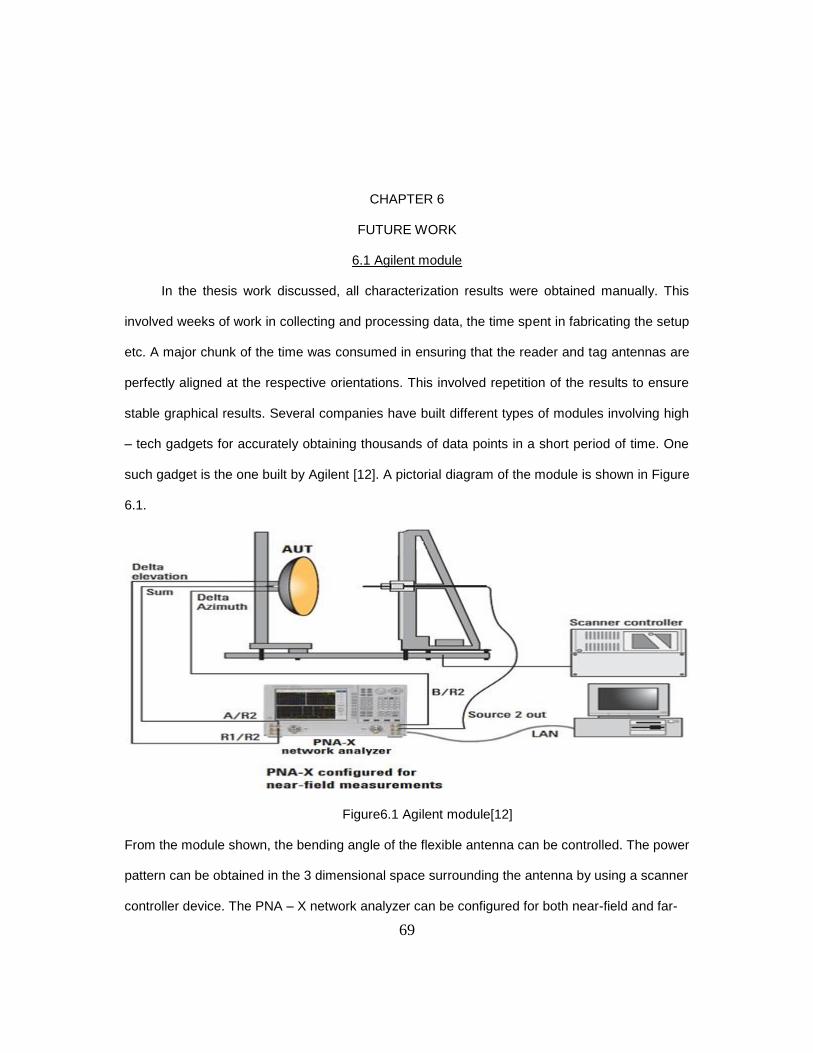
69
CHAPTER 6
FUTURE WORK
6.1 Agilent module
In the thesis work discussed, all characterization results were obtained manually. This
involved weeks of work in collecting and processing data, the time spent in fabricating the setup
etc. A major chunk of the time was consumed in ensuring that the reader and tag antennas are
perfectly aligned at the respective orientations. This involved repetition of the results to ensure
stable graphical results. Several companies have built different types of modules involving high
– tech gadgets for accurately obtaining thousands of data points in a short period of time. One
such gadget is the one built by Agilent [12]. A pictorial diagram of the module is shown in Figure
6.1.
Figure6.1 Agilent module[12]
From the module shown, the bending angle of the flexible antenna can be controlled. The power
pattern can be obtained in the 3 dimensional space surrounding the antenna by using a scanner
controller device. The PNA – X network analyzer can be configured for both near-field and far-

70
field measurements. The data collected by the network analyzer can then be stored in a
computer.
More than forty thousand data points can be obtained in a time interval of 10 to 20 minutes,
thus reducing the experimental time by one tenths. Also there is no human intervention, since
the experiments conducted are controlled automatically, thus improving the reliability of the
results obtained. Optimum Measurement sensitivity is a critical aspect for antenna
measurements, which is provided by the device.
In the future, reliable characterization experiments can be conducted using this module
for any kind of antenna in a short interval of time.
6.2 Stacked spiral antennas
By making use of flexible stacked antennas, the inductive power transfer can be
increased and the resonant magnetic coupling frequency can be reduced [10, 30], thereby
reducing the power absorbed by the body tissues and increasing the range of operation.
Characterization of these antennas is therefore important.
Figure 6.2 Stacked spiral antenna [10]

71
APPENDIX A
MATERIAL DATA SHEETS AND SPECIFICATIONS

72
A.1 KAPTON DATA SHEET
Kapton is a biocompatible material used as a substrate for fabrication of flexible antennas. Their
characteristics are discussed in Table 1, Table 2 and Table 3.
TABLE 1 Typical Electrical Properties of DuPont™ Kapton
® HN Film at 23°C (73°F), 50% RH
TABLE 2
Thermal Properties of DuPont™ Kapton® HN Film

73
TABLE 3
Physical Properties of DuPont™ Kapton® HN at 23°C (73°F)

74
A2. JVCC CFL-5CA COPPER FOIL TAPE (CONDUCTIVE ADHESIVE) SPECIFICATIONS
Adhesive: The bottom side of copper foil has conductive acrylic with the help of which it can
stick on any material
Carrier/Backing: copper foil
Release Liner: 60# paper
Thickness of tape: 3 mils (without liner) 1.6 mils (adhesive) 1.4 mils (carrier/backing)
Adhesion: 70 ounces per inch (to stainless steel)
Tensile Strength: 36 pounds per inch (longitudinal)
Service/Operating Temperature: up to 311°F
Elongation: 6%
Electrical Resistance: 0.003 Ohms/sq. in.
Certifications: File #130121, UL510, Section 4, MIL-T-47012
Core: 3" diameter neutral

75
APPENDIX B
MATLAB PROGRAMS

76
B1. CURRENTSHEET AND WHEELER FORMULAE
Matlab [14] codes were written for speedy calculation of inductances using formulas mentioned
in [17].
Currentsheet Function
function [Lgmd]=currentsheet(n,din,dout)
mu = 4*3.141592654*(10^-7);
c1 = 1.27;
c2 = 2.07;
c3 = 0.18;
c4 = 0.13;
davg = (dout+din)*0.5*(10^-3);
p = (dout - din)/(dout + din);
Lgmd = ((0.5*mu*(n^2)*davg*c1)*(loge(c2/p)+(c3*p)+(c4*(p^2))))*(10^6);
End
Wheeler Function
function [Lmw]=wheeler(n,din,dout)
k1 = 2.34;
k2 = 2.75;
davg = 0.5*(10^-3)*(dout+din);
p = (dout - din)/(dout + din);
Lmw = (k1*4*3.141592654*(10^-7)*(((n^2)*davg)/(1+(k2*p))))*(10^6);
End

77
B2. 3D PATTERN MATLAB PROGRAM
Also a matlab code was written to plot the 3D pattern graphs. The value of X axis and Y axis
was given as input. The value of Z axis which is the efficiency values at corresponding value of
X and Y are also given as input. The 3D pattern graph was then obtained using the in-built
matlab function -
plot3 (X,Y,Z)
legend (‘Ax, d = x cm’).

78
REFERENCES
[1] Upkar Varshney “Pervasive Healthcare and Wireless Health Monitoring”, Journal of Mobile
Networks and Applications, Volume 12, Issue 2-3, March 2007, Pages 113 – 127.
[2] Xiaoyu Liu, Fei Zhang, Steven A. Hackworth, Robert J. Sclabassi and Mingui Sun “Wireless
Power Transfer System Design for Implanted and Wom Devices”, Bioengineering Conference,
2009 IEEE 35th Annual North East.
[3] Anthony N. Laskovski, Tharaka Dissanayake and Mehmet R. Yuce “Wireless Power
Technology for Biomedical Implants”, Biomedical Engineering, pp 119 – 132.
[4] James W. (“Rus”) Healy “Antenna Here is a Dipole”, NJ2L.
[5] Thermpon Ativanichayaphong “Wireless Devices for Medical Applications”, ProQuest, The
University of Texas at Arlington, Electrical Engineering, December 2007.
[6] Anders J Johansson “Wireless Communication with Medical Implants : Antennas and
Propagation”, Department of Electroscience, Lund University, June 2004.
[7] Jaime Garnica, Joaquin Casanova, and Jenshan Lin “High Efficiency Midrange Wireless
Power Transfer System”, IMWS-IWPT2011 Proceedings.
[8] Teck Chuan Beh, Takehiro Imura, Masaki Kato, Yoichi Hori, “Wireless Power Transfer
System via Magnetic Resonant Coupling at Restricted Frequency Range – Fixing Resonace
Frequency With Impedance Matching”, University of Tokyo, 2010.
[9] Nathan O. Sokal “Class – E RF Power Amplifiers”, WA1HQC of Design Automation, Inc,
Jan/Feb 2001.
[10] Anthony Nikola Laskovski, Mehmet Rasit Yuce, and Tharaka Dissanayake, “Stacked
Spirals for Biosensor Telemetry”, IEEE Sensors Journal, VOL. 11, No. 6, June 2011.

79
[11] P. R. Troyk and G. A. DeMichele, “Inductively-coupled power and data link for neural
prostheses using a class-E oscillator and FSK modulation,” IEEE International Conference
Engineering in Medicine and Biology Society, Vol.4, pp.3376-3379, 2003.
[12] Agilent Technologies “Solutions for Antenna Characterization”
[13] Ansoft Corporation “Ansoft High Frequency Structure Simulator v10 User’s Guide”, 2005.
[14] Christos Xenophontos “A Beginner’s Guide to MATLAB”, Department of Mathematical
Sciences, Loyola College.
[15] Oleksiy Klymenko “UWB Receiver Frontend Design with ADS”, ADS User Group Meeting,
IHP, Frankfurt, Germany, pp 13 – 15, May 14 & 15, 2009.
[16] Uei – Ming Jow, Maysam Ghovanloo “Modeling and Optimization of Printed Spiral Coils in
Air, Saline, and Muscle Tissue Environments”, IEEE Transactions on Biomedical Circuits and
Systems, Vol . 3, No. 5, October 2009.
[17] Sunderajan S.Mohan, Maria del Mar Hershenson, Stephen P. Boyd, and Thomas H.Lee
"Simple Accurate Expressions for Planar Spiral Inductances", IEEE Journal of Solid-State
Circuits, Vol. 34, No. 10, October 1999.
[18] AutoDesk Official Training Guide “Autocad 2010 Volume 1”, April 2009.
[19] AutoDesk Official Training Guide “Autocad 2010 Volume 2”, April 2009.
[20] AutoDesSys “Bonzai 3d Online Manual”.
[21] http: www.antenna-theory.com.
[22] Constantine A. Balanis "Antenna Theory: Analysis and Design", 3rd Edition, 1999.
[23] Enver G. Kilinc, Catherine Dehollain, "Design and Optimization of Inductive Power
Transmission for Implantable Sensor System", Symbolic and Numerical Methods, Modeling and
Applications to Circuit Design (SM2ACD), 2010 XIth International Workshop on 4-6 Oct, 2010.
[24] Eui-Jung Yun, Jae-Wook Kim, Won-Gook Lee, Young-Jin Kim, Hyeong-Sik Park "Analytical
estimation of high-frequency properties of RF micro-inductors prepared by direct-write
techniques", Springer Science + Business Media, LLC 2007.

80
[25] M. Bartek, S.M. Sinaga, J.N. Burghartz "Influence of via-connections on electrical
performance of vertically-spaced RF passives", Electronic Components and Technology
Conference, 2005.
[26] Amal Zaki "Design and Fabrication of High-Q Spiral Inductors Using MEMS Technology",
Proceedings of the 4th WSEAS Int. Conference on Electromagnetics, Wireless and Optical
Communications, Venice, Italy, November 20-22, 2006.
[27] Jr-Wei Lin, C. C. Chen, and Yu-Ting Cheng, Member, IEEE "A Robust High-Q
Micromachined RF Inductor for RFIC Applications", IEEE Transactions on Electron Devices,
Vol. 52, No. 7, July 2005.
[28] Kenichi Okada and Kazuya Masu "Modeling of Spiral Inductors", Tokyo Institute of
Technology, Japan.
[29] Steve McFee and Dennis Giannacopoulos, "Introduction to Adaptive Finite Element
Analysis for Electromagnetic Simulations", Technical Article, Department of Electrical &
Computer Engineering, McGill University, Canada.
[30] Anthony Nikola Laskovski, Mehmet Rasit Yuce, Tharaka Dissanayake "Stacked Spirals for
Biosensor Telemetry", IEEE Sensors Journal, Vol. 11, NO. 6, June 2011.
[31] http:www.google.com

81
BIOGRAPHICAL INFORMATION
Safwan Ahmed Muneer was born in Bangalore, Karnataka, India. He obtained his
Bachelor’s degree in Electronics and Communication Engineering in 2009, from Visweswaraiah
Technological University, Belgaum, Karnataka, India. He has worked towards his Master of
Science in Electrical Engineering in The University of Texas at Arlington since August 2010. His
Research areas include Antenna Design and Wireless radio frequency Communication.
Related Documents