2018-01-17 1 Wireless Communication Channels Lecture 3: Fading EITN85, FREDRIK TUFVESSON ELECTRICAL AND INFORMATION TECHNOLOGY Wireless Communication Channels 2 Fading – Statistical description of the wireless channel • Why statistical description • Large scale fading • Fading margin • Small scale fading – without dominant component – with dominant component • Statistical models • Measurement example 2016-01-22 VT 2018

Welcome message from author
This document is posted to help you gain knowledge. Please leave a comment to let me know what you think about it! Share it to your friends and learn new things together.
Transcript

2018-01-17
1
Wireless Communication ChannelsLecture 3: Fading
EITN85, FREDRIK TUFVESSON
ELECTRICAL AND INFORMATION TECHNOLOGY
Wireless Communication Channels 2
Fading – Statistical description of thewireless channel
• Why statistical description• Large scale fading• Fading margin• Small scale fading
– without dominant component– with dominant component
• Statistical models• Measurement example
2016-01-22VT 2018
2018-01-17
2
VT 2018 Wireless Communication Channels 3
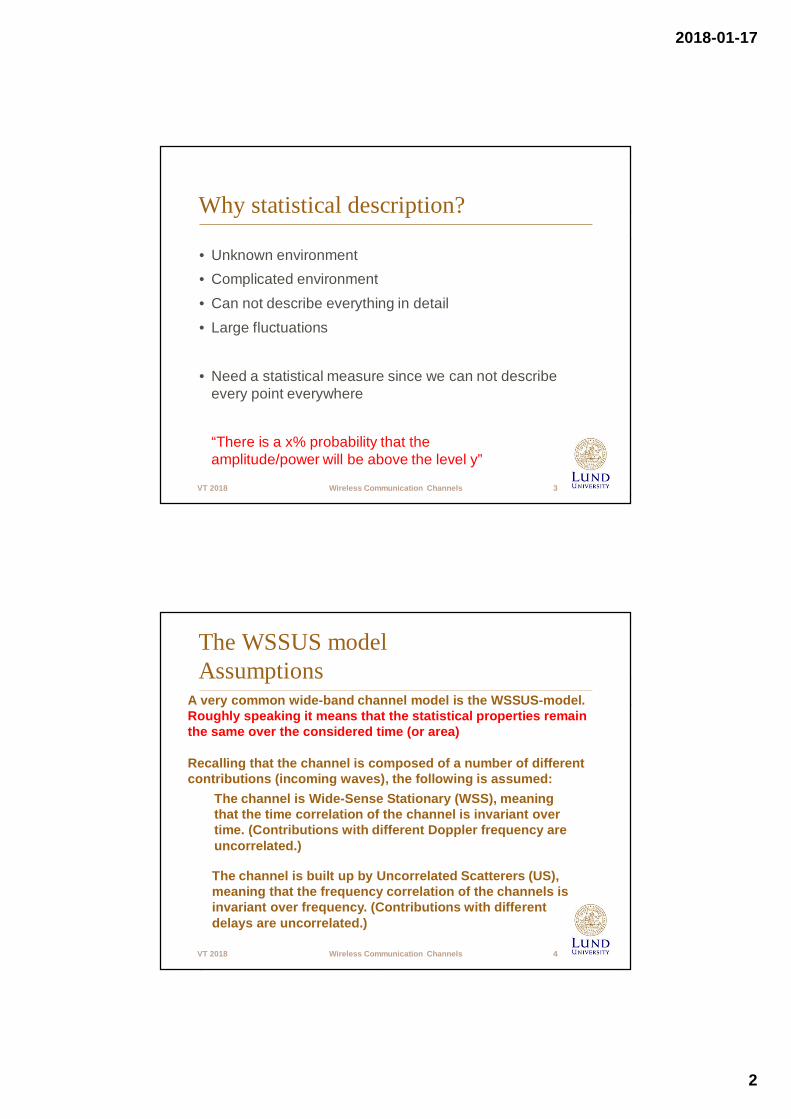
Why statistical description?
• Unknown environment• Complicated environment• Can not describe everything in detail• Large fluctuations
• Need a statistical measure since we can not describeevery point everywhere
“There is a x% probability that theamplitude/power will be above the level y”
VT 2018 Wireless Communication Channels 4
The WSSUS modelAssumptions
A very common wide-band channel model is the WSSUS-model.Roughly speaking it means that the statistical properties remainthe same over the considered time (or area)
Recalling that the channel is composed of a number of differentcontributions (incoming waves), the following is assumed:
The channel is Wide-Sense Stationary (WSS), meaningthat the time correlation of the channel is invariant overtime. (Contributions with different Doppler frequency areuncorrelated.)
The channel is built up by Uncorrelated Scatterers (US),meaning that the frequency correlation of the channels isinvariant over frequency. (Contributions with differentdelays are uncorrelated.)
2018-01-17
3
VT 2018 Wireless Communication Channels 5
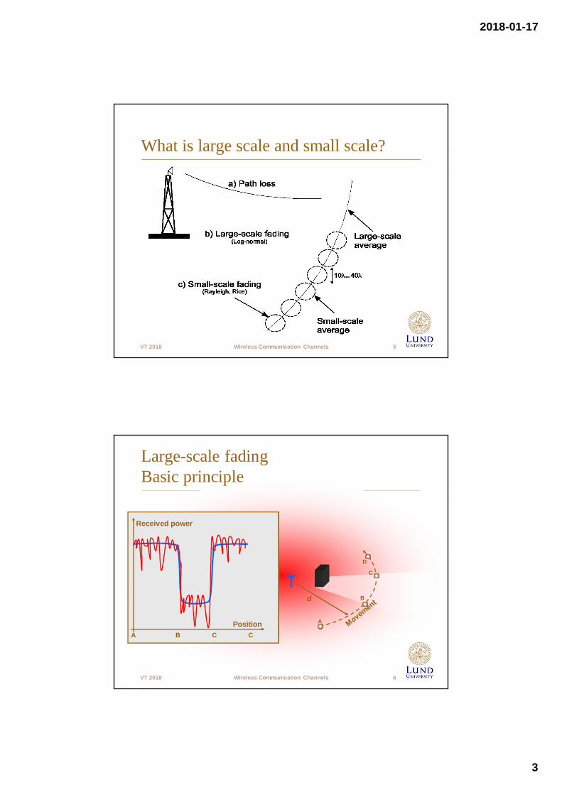
What is large scale and small scale?
VT 2018 Wireless Communication Channels 6
Large-scale fadingBasic principle
d
Received power
PositionA B C C
A
B
C
D
2018-01-17
4
VT 2018 Wireless Communication Channels 7
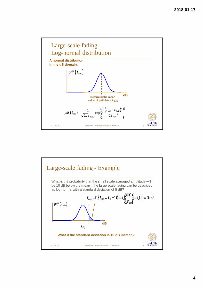
Large-scale fadingLog-normal distribution
A normal distributionin the dB domain.
( ) ( )2| 0|
| 2||
1 exp22
dB dBdB
F dBF dB
L Lpdf L
sps
æ ö-ç ÷= -ç ÷è ø
dBDeterministic meanvalue of path loss, L0|dB
( )|dBpdf L
VT 2018 Wireless Communication Channels 8
Large-scale fading - Example
What is the probability that the small scale averaged amplitude willbe 10 dB below the mean if the large scale fading can be describedas log-normal with a standard deviation of 5 dB?
dB
( )|dBpdf L
What if the standard deviation is 10 dB instead?
{ } ( ) 02.021010Pr 0 »=÷÷ø
öççè
æ=+³= QQLLP
dBdBout s
0L
2018-01-17
5
VT 2018 Wireless Communication Channels 9
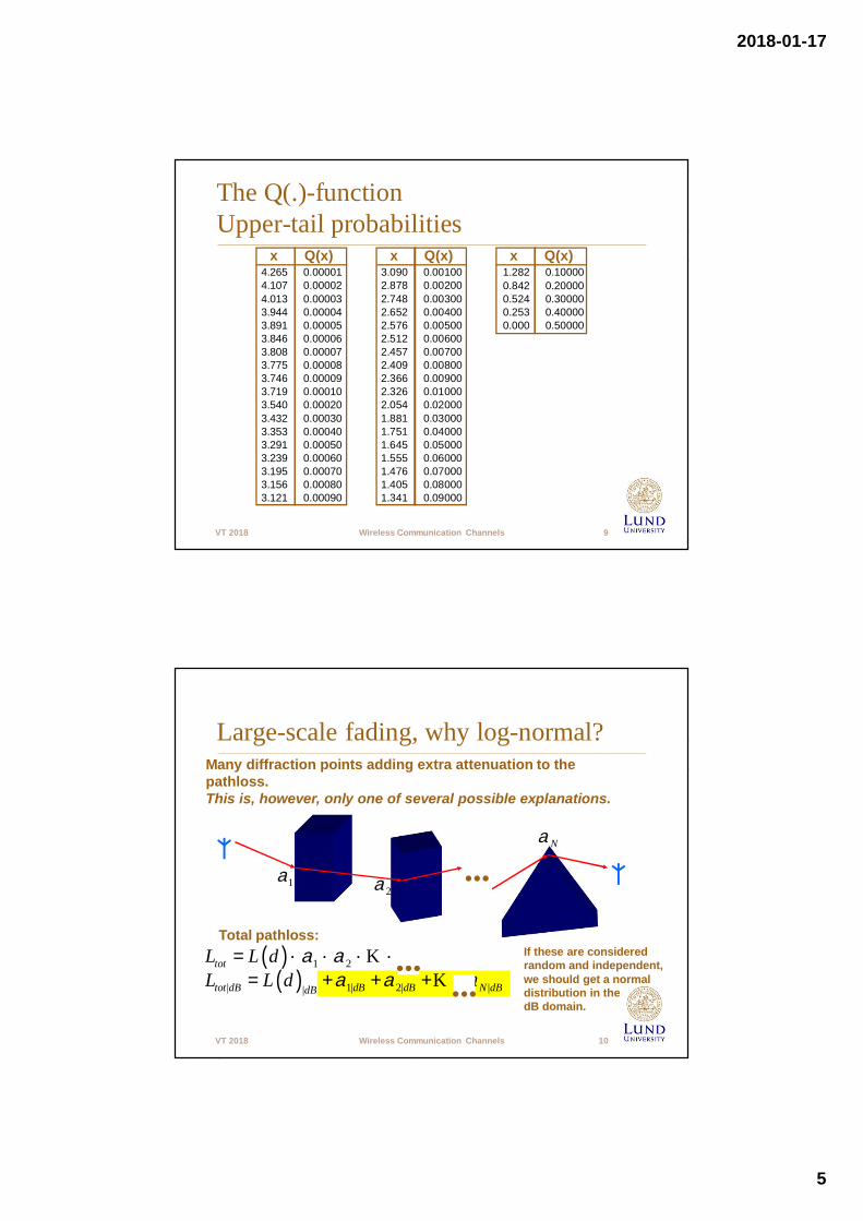
The Q(.)-functionUpper-tail probabilities
4.265 0.000014.107 0.000024.013 0.000033.944 0.000043.891 0.000053.846 0.000063.808 0.000073.775 0.000083.746 0.000093.719 0.000103.540 0.000203.432 0.000303.353 0.000403.291 0.000503.239 0.000603.195 0.000703.156 0.000803.121 0.00090
3.090 0.001002.878 0.002002.748 0.003002.652 0.004002.576 0.005002.512 0.006002.457 0.007002.409 0.008002.366 0.009002.326 0.010002.054 0.020001.881 0.030001.751 0.040001.645 0.050001.555 0.060001.476 0.070001.405 0.080001.341 0.09000
1.282 0.100000.842 0.200000.524 0.300000.253 0.400000.000 0.50000
x Q(x) x Q(x) x Q(x)
VT 2018 Wireless Communication Channels 10
If these are consideredrandom and independent,we should get a normaldistribution in thedB domain.
Large-scale fading, why log-normal?
1a2a
Na
Many diffraction points adding extra attenuation to thepathloss.This is, however, only one of several possible explanations.
Total pathloss:( ) 1 2tot NL L d a a a= ´ ´ ´ ´K
( )| 1| 2| ||tot dB dB dB N dBdBL L d a a a= + + + +K
2018-01-17
6
VT 2018 Wireless Communication Channels 11
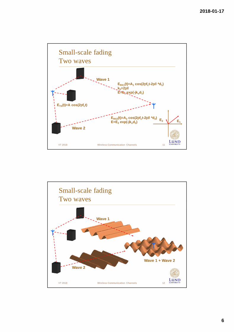
Small-scale fadingTwo waves
Wave 2
Wave 1
ETX(t)=A cos(2pfct)
ERX1(t)=A1 cos(2pfct-2p/l*d1)k0=2p/lE=E1 exp(-jkod1)
ERX2(t)=A2 cos(2pfct-2p/l*d2)E=E2 exp(-jkod2) E1
E2
VT 2018 Wireless Communication Channels 12
Small-scale fadingTwo waves
Wave 1 + Wave 2
Wave 2
Wave 1
2018-01-17
7
VT 2018 Wireless Communication Channels 13
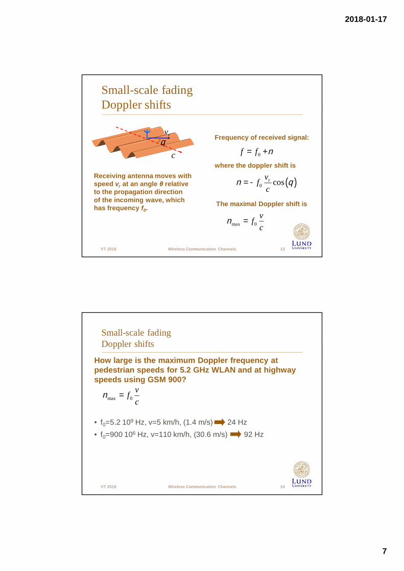
Small-scale fadingDoppler shifts
c
rvq
0f f n= +
Frequency of received signal:
( )0 cosrvfc
n q= -
where the doppler shift isReceiving antenna moves withspeed vr at an angle θ relativeto the propagation directionof the incoming wave, whichhas frequency f0.
The maximal Doppler shift is
max 0vfc
n =
VT 2018 Wireless Communication Channels 14
Small-scale fadingDoppler shifts
• f0=5.2 109 Hz, v=5 km/h, (1.4 m/s) 24 Hz• f0=900 106 Hz, v=110 km/h, (30.6 m/s) 92 Hz
max 0vfc
n =
How large is the maximum Doppler frequency atpedestrian speeds for 5.2 GHz WLAN and at highwayspeeds using GSM 900?
2018-01-17
8
VT 2018 Wireless Communication Channels 15
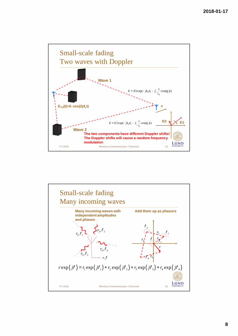
Small-scale fadingTwo waves with Doppler
0 2 20
2exp( cos( ) )cvE E jk d f tc
q= - -
Wave 2
Wave 1
ETX(t)=A cos(2pfct)
0 1 10
1exp( cos( ) )cvE E jk d f tc
q= - -
v
E1E2
The two components have different Doppler shifts!The Doppler shifts will cause a random frequencymodulation
VT 2018 Wireless Communication Channels 16
Small-scale fadingMany incoming waves
1 1,r f 2 2,r f
3 3,r f4 4,r f
,r f
( ) ( ) ( ) ( ) ( )1 1 2 2 3 3 4 4exp exp exp exp expr j r j r j r j r jf f f f f= + + +
1r1f
2r 2f
3r
3f
4r4f
r
f
Many incoming waves withindependent amplitudesand phases
Add them up as phasors
2018-01-17
9
VT 2018 Wireless Communication Channels 17
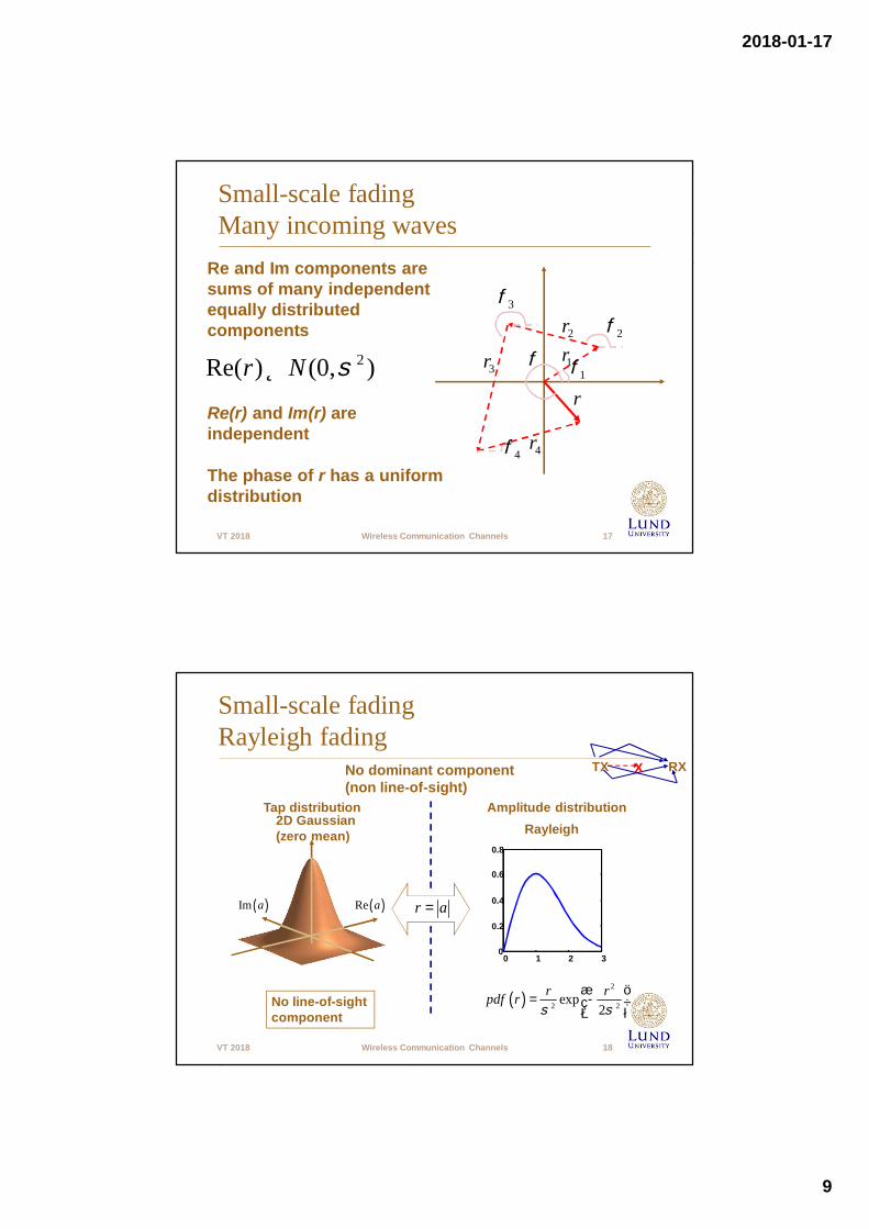
Small-scale fadingMany incoming waves
1r1f
2r 2f
3r
3f
4r4f
r
f
Re and Im components aresums of many independentequally distributedcomponents
Re(r) and Im(r) areindependent
The phase of r has a uniformdistribution
2Re( ) (0, )r N sÎ
VT 2018 Wireless Communication Channels 18
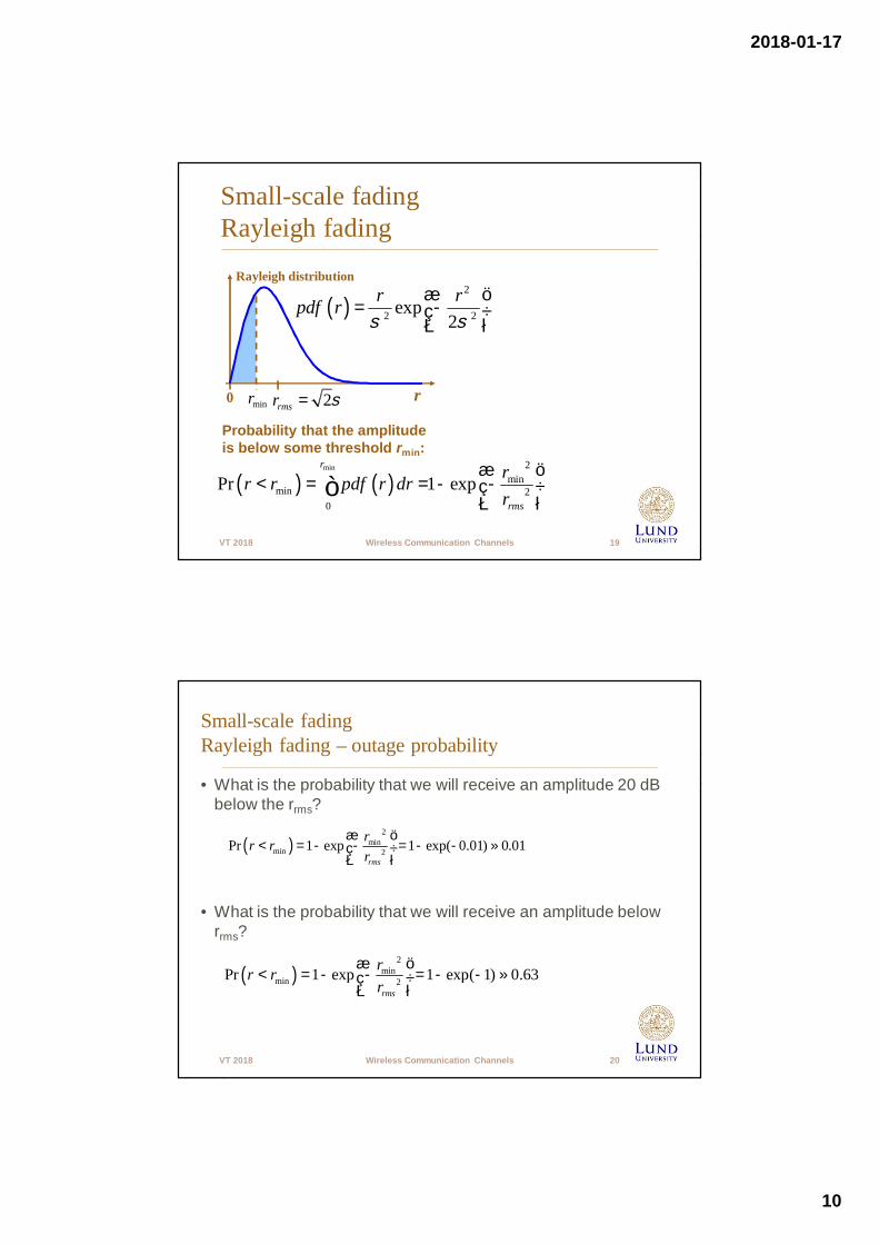
Small-scale fadingRayleigh fading
No dominant component(non line-of-sight)
2D Gaussian(zero mean)
Tap distribution
( )2
2 2exp2
r rpdf rs s
æ ö= -ç ÷
è ø
Amplitude distributionRayleigh
0 1 2 30
0.2
0.4
0.6
0.8
r a=
No line-of-sightcomponent
TX RXX
( )Im a ( )Re a
2018-01-17
10
VT 2018 Wireless Communication Channels 19
Small-scale fadingRayleigh fading
minr
( ) ( )min 2
minmin 2
0
Pr 1 expr
rms
rr r pdf r drr
æ ö< = = - -ç ÷
è øò
Probability that the amplitudeis below some threshold rmin:
0 r
Rayleigh distribution
2rmsr s=
( )2
2 2exp2
r rpdf rs s
æ ö= -ç ÷
è ø
VT 2018 Wireless Communication Channels 20
Small-scale fadingRayleigh fading – outage probability
• What is the probability that we will receive an amplitude 20 dBbelow the rrms?
• What is the probability that we will receive an amplitude belowrrms?
( )2
minmin 2Pr 1 exp 1 exp( 0.01) 0.01
rms
rr rr
æ ö< = - - = - - »ç ÷
è ø
( )2
minmin 2Pr 1 exp 1 exp( 1) 0.63
rms
rr rr
æ ö< = - - = - - »ç ÷
è ø
2018-01-17
11
VT 2018 Wireless Communication Channels 21
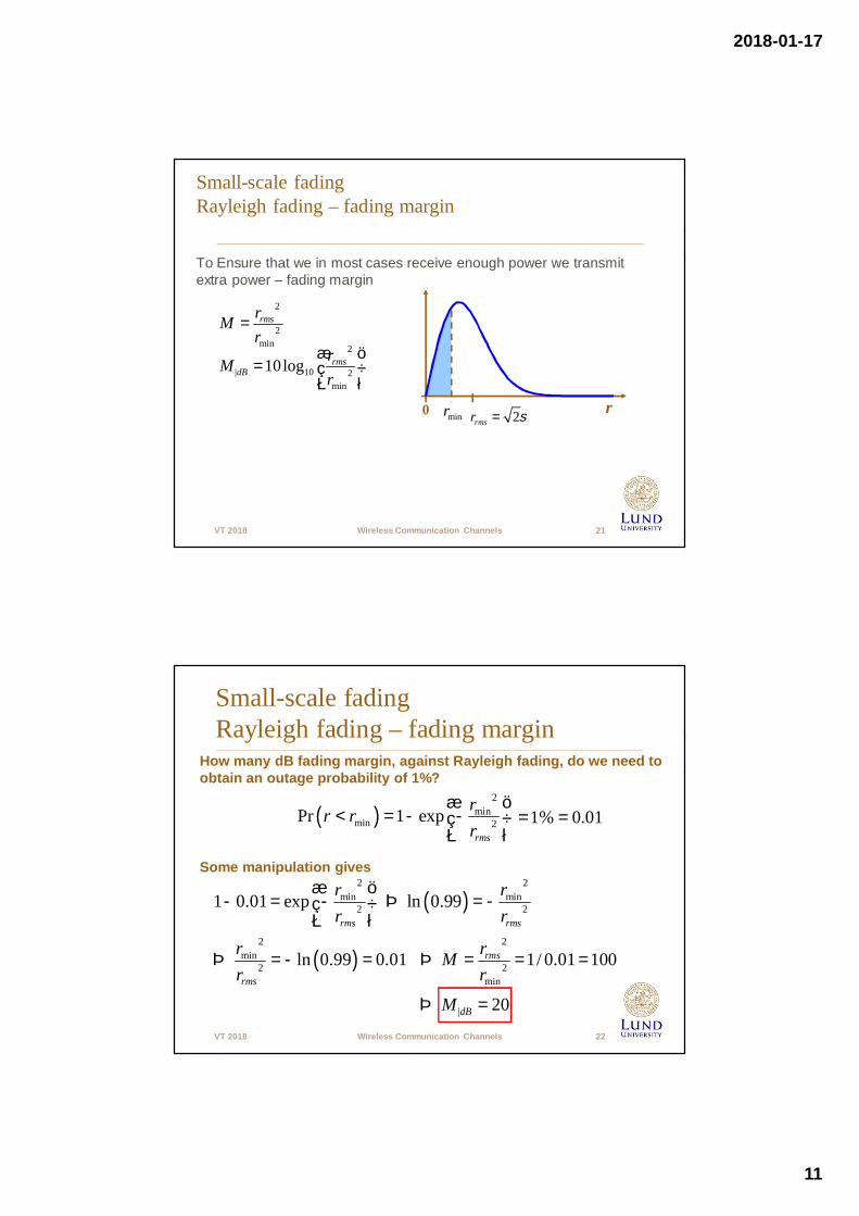
Small-scale fadingRayleigh fading – fading margin
To Ensure that we in most cases receive enough power we transmitextra power – fading margin
2
2min
rmsrMr
=2
| 10 2min
10log rmsdB
rMr
æ ö= ç ÷
è ø
minr0 r2rmsr s=
VT 2018 Wireless Communication Channels 22
Small-scale fadingRayleigh fading – fading margin
How many dB fading margin, against Rayleigh fading, do we need toobtain an outage probability of 1%?
( )2
minmin 2Pr 1 exp
rms
rr rr
æ ö< = - -ç ÷
è ø1% 0.01= =
Some manipulation gives2
min21 0.01 exp
rms
rr
æ ö- = -ç ÷
è ø( )
2min
2ln 0.99rms
rr
Þ = -
( )2
min2 ln 0.99 0.01
rms
rr
Þ = - =2
2min
1/ 0.01 100rmsrMr
Þ = = =
| 20dBMÞ =
2018-01-17
12
VT 2018 Wireless Communication Channels 23
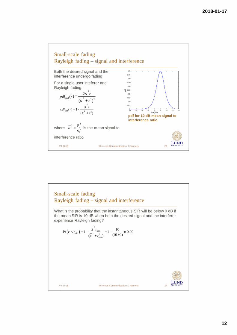
Small-scale fadingRayleigh fading – signal and interference
Both the desired signal and theinterference undergo fading
For a single user inteferer andRayleigh fading:
where is the mean signal to
interference ratio
2
2 2 2
2( )( )
SIRrpdf rr
s
s=
+2
2 2( ) 1
( )SIR
rcdf rr
s
s= -
+
22 22
1
ss
s=
-20 -15 -10 -5 0 5 10 15 200
0.05
0.1
0.15
0.2
0.25
0.3
0.35
0.4
0.45
0.5
SIR(dB)
pdf for 10 dB mean signal tointerference ratio
VT 2018 Wireless Communication Channels 24
Small-scale fadingRayleigh fading – signal and interference
What is the probability that the instantaneous SIR will be below 0 dB ifthe mean SIR is 10 dB when both the desired signal and the interfererexperience Rayleigh fading?
( )2
minmin 2 2
min
10Pr 1 1 0.09(10 1)( )
rr rr
s
s< = - = - »
++
2018-01-17
13
VT 2018 Wireless Communication Channels 25
Small-scale fadingone dominating componentIn case of Line-of-Sight (LOS) one component dominates.
• Assume it is aligned with the real axis
• The recieved amplitude has now a Ricean distributioninstead of a Rayleigh
– The fluctuations are smaller
– The phase is dominated by the LOS component
– In real cases the mean propagation loss is often smaller dueto the LOS
• The ratio between the power of the LOS component and thediffuse components is called Ricean K-factor
2Re( ) ( , )r N A sÎ 2Im( ) (0, )r N sÎ
2
2Power in LOS component
Power in random components 2Aks
= =
VT 2018 Wireless Communication Channels 26
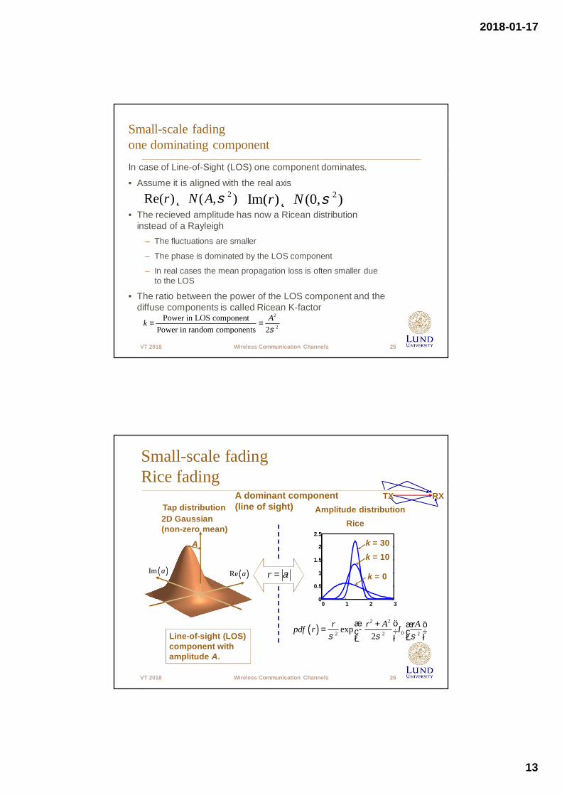
Small-scale fadingRice fading
A dominant component(line of sight)
2D Gaussian(non-zero mean)
Tap distribution
A
Line-of-sight (LOS)component withamplitude A.
( )2 2
02 2 2exp2
r r A rApdf r Is s s
æ ö+ æ ö= -ç ÷ ç ÷è øè ø
Amplitude distributionRice
r a=
0 1 2 30
0.5
1
1.5
2
2.5k = 30k = 10
k = 0
TX RX
( )Im a ( )Re a
2018-01-17
14
VT 2018 Wireless Communication Channels 27
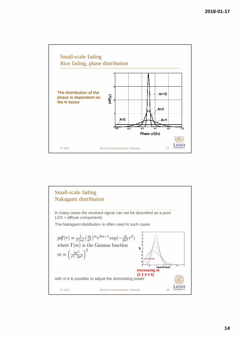
Small-scale fadingRice fading, phase distribution
The distribution of thephase is dependent onthe K-factor
VT 2018 Wireless Communication Channels 28
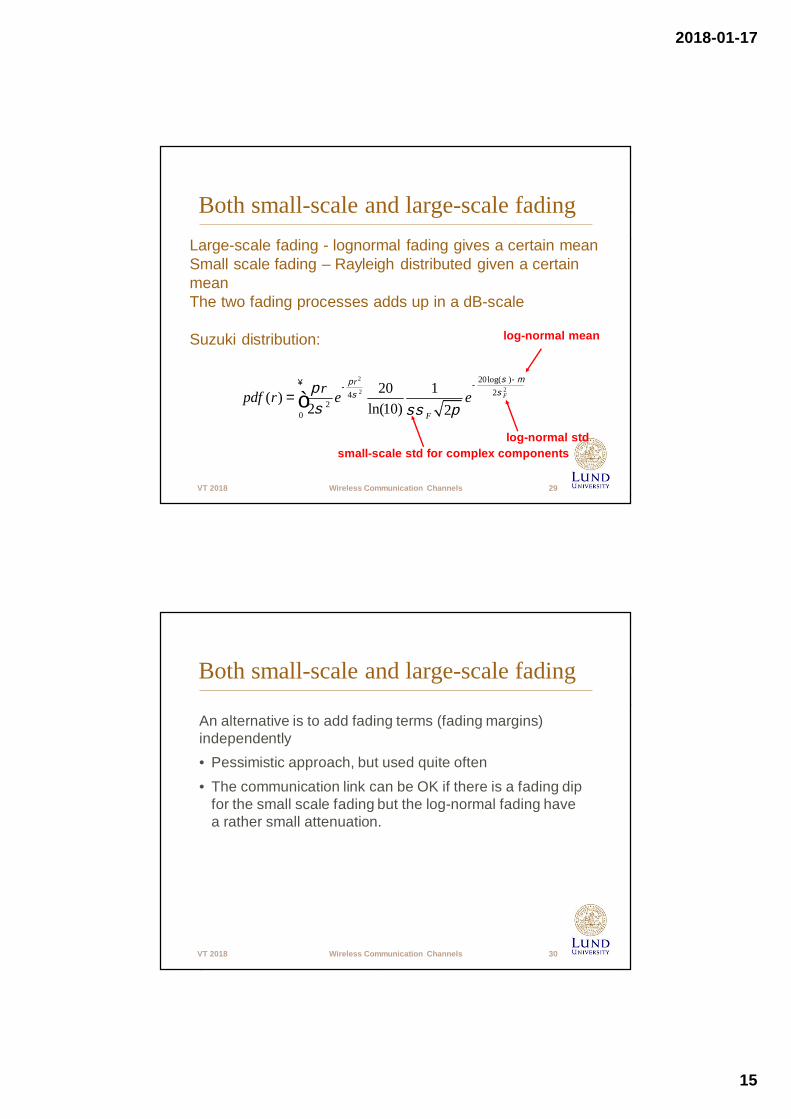
Small-scale fadingNakagami distribution
In many cases the received signal can not be described as a pureLOS + diffuse components
The Nakagami distribution is often used in such cases
with m it is possible to adjust the dominating power
increasing m{1 2 3 4 5}
2018-01-17
15
VT 2018 Wireless Communication Channels 29
Both small-scale and large-scale fadingLarge-scale fading - lognormal fading gives a certain meanSmall scale fading – Rayleigh distributed given a certainmeanThe two fading processes adds up in a dB-scale
Suzuki distribution:
2
22
20log( )24
20
20 1( )2 ln(10) 2
F
r
F
rpdf r e es mp
ssps ss p
-¥ --= ò
log-normal std
log-normal mean
small-scale std for complex components
VT 2018 Wireless Communication Channels 30
Both small-scale and large-scale fading
An alternative is to add fading terms (fading margins)independently• Pessimistic approach, but used quite often• The communication link can be OK if there is a fading dip
for the small scale fading but the log-normal fading havea rather small attenuation.
2018-01-17
16
VT 2018 Wireless Communication Channels 31
Some special casesRayleigh fading
Rice fading, K=0
Rice fading with K=0 becomes Rayleigh
Nakagami, m=1
Nakagami with m=1 becomes Rayleigh
( )2
2 2exp2
r rpdf rs s
æ ö= -ç ÷
è ø
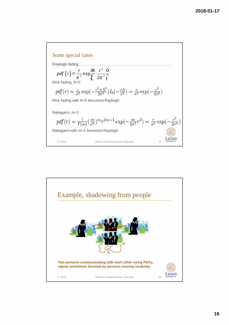
Example, shadowing from people
VT 2018 Wireless Communication Channels 32
Two persons communicating with each other using PDAs,signal sometimes blocked by persons moving randomly
2018-01-17
17
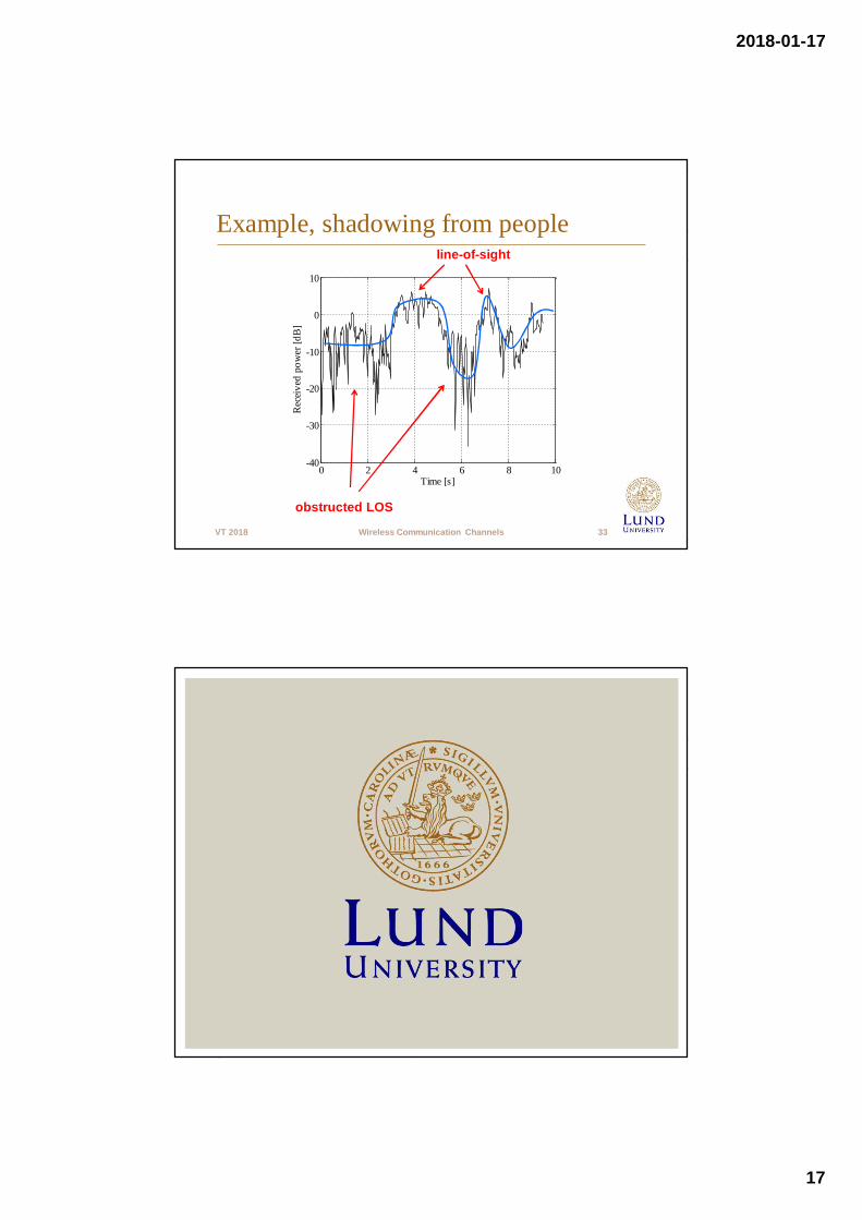
Example, shadowing from people
0 2 4 6 8 10-40
-30
-20
-10
0
10
Time [s]
Rec
eive
dpo
wer
[dB
]
VT 2018 Wireless Communication Channels 33
line-of-sight
obstructed LOS
Related Documents

![[PPT]Wireless Channels: Small Scale Fading (Multipath …web2.uwindsor.ca/.../uwireless/channels_smallscalefading.ppt · Web viewWireless Channels: Small Scale Fading (Multipath and](https://static.cupdf.com/doc/110x72/5b3cfdd57f8b9a0e628df536/pptwireless-channels-small-scale-fading-multipath-web2-web-viewwireless.jpg)


