Window double barrier options - HAL archive ouverte · Pelsser (2000) studies binary double barrier options including a rebate paid when either one of the barriers is hit. Based on

HAL Id: hal-00924247https://hal.archives-ouvertes.fr/hal-00924247

Submitted on 6 Jan 2014

HAL is a multi-disciplinary open accessarchive for the deposit and dissemination of sci-entific research documents, whether they are pub-lished or not. The documents may come fromteaching and research institutions in France orabroad, or from public or private research centers.

L’archive ouverte pluridisciplinaire HAL, estdestinée au dépôt et à la diffusion de documentsscientifiques de niveau recherche, publiés ou non,émanant des établissements d’enseignement et derecherche français ou étrangers, des laboratoirespublics ou privés.

Window double barrier optionsTristan Guillaume

To cite this version:Tristan Guillaume. Window double barrier options. Review of Derivatives Research, Springer Verlag,2003, 6, pp.47-75. �hal-00924247�

1

WINDOW DOUBLE BARRIER OPTIONS

Revised version, 2005

Originally published in Review of Derivatives Research, 2003, (6), 47-75

TRISTAN GUILLAUME

Université de Cergy-Pontoise, Laboratoire Thema, 33 boulevard du port, F-95011 Cergy-Pontoise

Cedex, France

Abstract. This paper examines a path-dependent contingent claim called the window double barrier

option, including standard but also more exotic features such as combinations of single and double

barriers. Price properties and hedging issues are discussed, as well as financial applications. Explicit

formulae are provided, along with simple techniques for their implementation. Numerical results show

that they compare very favourably with alternative pricing approaches in terms of accuracy and

efficiency.

Keywords : option, barrier, double barrier, window, pricing, hedging, numerical integration,

dimension.

JEL classification : G13

2

Introduction

In conjunction with their growing popularity in the OTC markets, double barrier options have

gradually moved to the forefront of derivatives research. The main developments in the literature

pertaining to their analytical valuation can be briefly outlined. Based on a generalisation of the Levy

formula, Kunitomo and Ikeda (1992) provide a valuation formula for double barrier options with

payoff restricted by two curved absorbing boundaries assumed to be exponential functions of time.

Geman and Yor (1996) make use of the Cameron-Martin theorem to derive the Laplace transform of

the double barrier option price with respect to its expiry date. Inversion of this transform can be done

numerically using the Fast Fourier transform (Geman and Eydeland, 1995), or analytically using the

Cauchy Residue theorem (Schröder, 2000). Expressing double barrier option values as a linear

combination of sine functions, Bhagavatula and Carr (1995) handle time-dependent parameters.

Analytically solving the Black-Scholes partial differential equation with the appropriate boundary

conditions, Hui (1997) prices front-end and rear-end double barrier options, featuring early-ending

and forward-start monitoring respectively. Combining Laplace transform and contour integration,

Pelsser (2000) studies binary double barrier options including a rebate paid when either one of the

barriers is hit. Based on the first passage densities of Brownian motion derived by Sidenius (1998),

Luo (2001) considers ordered double barrier options in which the payoff is contingent on whether the

lower or the upper barrier is hit first.

Even though research on double barrier options has been growing steadily, there is still an

important type of contract that admits no explicit solution : window double barrier options. In their

standard form, they feature a double barrier whose monitoring starts after the contract initiation and

terminates before the contract expiry. In this respect, they can be regarded as an extension of the

forward-start and early-ending double barrier options studied by Hui (1997). A more exotic variation

is the partial window double barrier option, featuring combinations of single barriers before and after

the double barrier. The benefits of these contracts are manifold. Window double knock-out options are

cheaper than vanilla options and less risky than standard double knock-out options. Window double

knock-in options have greater leverage than standard double knock-in options. Whether they are

knock-in or knock-out, window double barrier options are more flexible than standard double barrier

options, allowing to match more closely the hedging needs or the speculative views of market

participants.

3

However, the expansion of these contracts in the marketplace is contingent on the ability to obtain

exact prices and hedging parameters in trading time. In this respect, closed form formulae would be

most welcome, at least as benchmarks to test more general numerical schemes allowing to relax

restrictive modeling assumptions. An analytical solution to such a valuation problem involves the

calculation of several distributions of joint extrema of geometric Brownian motion that are currently

unknown. It also implies to cope with a dimension issue, as the values of standard and partial window

double barrier options can only be formulated in terms of multiple integrals.

This paper provides two exact formulae that suffice to span all kinds of standard and partial window

double barrier options. It also shows how to implement them with high accuracy and efficiency. The

valuation framework is the classical equivalent martingale measure one (Harrison and Pliska, 1981),

unlike the partial differential equation approach used by Bhagavatula and Carr (1995) and Hui (1997),

or the Laplace transform approach followed by Geman and Yor (1996) and Pelsser (2000). It is shown

that by repeatedly conditioning and using the Markov property of Brownian motion, the appropriate

discounted expectations can be rewritten in terms of tractable multiple integrals. The dimension issue

is dealt with by using convolutions of the multivariate standard normal distribution that allow to

dispose of most correlation coefficients.

Section 1 presents details on window double barrier options and their applications, along with the

formula for standard-type contracts. Section 2 studies price behavior for various parameters, based on

a comparison with other existing contracts. Section 3 discusses hedging issues. Appendix A gives

detailed proof of the valuation formula for standard window double barrier options as well as a

numerical implementation rule. Appendix B provides the valuation formula for partial window double

barrier options, along with an appropriate numerical implementation technique.

1. The case for window double barrier options

Option users basically break down into hedgers and speculators. The former seek to reduce

the uncertainty caused by the fluctuations in financial prices. It is well-known that, compared to

alternative derivatives such as forward and futures contracts or swaps, options are very flexible and

have the remarkable property to insure investors against adverse price changes while allowing them to

benefit from favorable movements. The downside is that vanilla options are expensive. One way to

cut the cost of hedging is to eliminate unlikely scenarios. This can be achieved by purchasing barrier

options, especially those featuring a double barrier because only they allow not to pay for part of the

4

upward potential and part of the downward potential of the underlying. These contracts are now

heavily traded, particularly in the foreign exchange markets. They are also embedded in a lot of

popular structured derivatives in equity and interest rate markets, such as convertible/callable bonds

and stock warrants. However, holders of knock-out options face the possibility of losing their

insurance before expiry. Investors may even never become insured if their contract is contingent to a

knock-in provision. These risks sometimes motivate the introduction of a rebate as a form of

compensation. The danger of knocking-out could be reduced by setting the upper and the lower

barrier far away from the underlying spot price. Conversely, the risk of never knocking-in could be

diminished by locating the double barrier very near the spot price. But, in both cases, the premium

then quickly rises to that of a vanilla option at a speed proportional to the volatility of the underlying.

Given that hedgers do not often have precise views on the market direction over the entire option life

(otherwise, they would not hedge !), an alternative way of limiting the risk of sudden death inherent in

knock-out contracts consists in activating the double barrier during only a fraction of the option life,

while avoiding exposure when there is greater uncertainty as to the volatility of the underlying. Partial

double barrier options are supposed to meet this requirement, but they do so too rigidly, since the

activation period must either start at the contract’s inception or end at expiry. These conditions

imposed on investors may not suit their needs. Window double barrier options, on the contrary,

provide investors with all the flexibility they can expect from a customized exotic structure. In their

standard form, these contracts are call or put options with a knock-out or a knock-in double barrier

whose monitoring begins after the contract initiation and terminates before expiry. In other words, the

location of the double barrier can be chosen anywhere during the option life.

Window double barrier options include partial and standard double barrier options as special cases.

They enable investors to benefit from substantial premium discounts compared to vanilla or single

barrier contracts, while allowing them to reduce and customize their risk exposure compared to

standard or partial double barrier contracts. Suppose that an investor wants to hedge her or his

portfolio of stocks at the lowest possible cost using options. If, for example, quarterly earnings are

expected soon, she or he might prefer not to bet on the portfolio’s worth in the short term.

Furthermore, this cautious investor presumably does not want to risk losing her or his insurance at the

end of the option life because of a short price spike through the barrier near expiry. Then, it is easily

argued that only a window double barrier option can precisely match this investor’s preferences.

Window-type contracts are attractive not only to investors concerned with hedging but also to

those willing to speculate on market movements. Indeed, they provide outstanding leverage. Suppose,

for example, that an investor is bullish on the currency of a country A in the medium/long term. She

or he is willing to take a long position in a call option but finds it much too expensive in the current

5

market conditions. If there is a known event, during this period of time, that will almost certainly

increase volatility in the currency, she or he can turn to a knock-in option. It could be, for instance,

elections in country A scheduled in several months, especially if the contenders have opposite stances

on monetary and fiscal policy. Purchasing a single barrier knock-in option is a very risky strategy

because neither the results of the elections nor the reaction of the markets to them can be known ahead

of time. The choice of a standard or partial double barrier knock-in option solves this problem, but not

in an optimal manner, since the investor has to pay for activating rights during periods of time when

she or he does not want them.

Window double barrier options also have a number of desirable properties for option writers.

Some of them are shared by all double barrier contracts, such as the capacity to limit both downside

and upside risk, in contrast to the unlimited liability typical of vanilla options or the semi-unlimited

liability typical of single barrier options. Others are specific to window double barrier options. First,

option writers receive a higher premium than that of a standard double knock-out contract. Second,

hedging difficulties are mitigated since the possibility of breaching the barrier is monitored during

only a fraction of the option life. Section 3 discusses this point in more detail. Third, linear

combinations of window and forward-start/early-ending double barrier options could be used to

replicate exotic structures that are popular but difficult to value and to hedge, such as the so-called

“corridor” or “hot-dog” contracts, which involve sequences of double barriers in time.

As mentioned in the introduction of this paper, increased trading in window double barrier

options in the marketplace crucially depends on the ability to obtain exact prices and hedge

parameters in real time. Assuming that the underlying asset follows a geometric Brownian motion

with riskless rate r , volatility s and dividend rate d , the following closed form formula then solves

the valuation problem :

Proposition 1 :

The no-arbitrage value V of a standard window double knock-out option is given by:

dd s q m m 3 3

0 01 2 1 2 3, , , , , , , , , rt tV S K H H r t t t e K e S (1)

where :

1H is the lower part of the double barrier, 2H is the upper part of the double barrier, 0S is the

underlying asset spot value, K is the strike price, 0 0t is the contract’s inception, 1t is the time at

which monitoring of the double barrier starts with 01t t , 2t is the time at which monitoring of the

double barrier ends with 2 1t t , 3t is the option expiry with 3 2t t ,

6

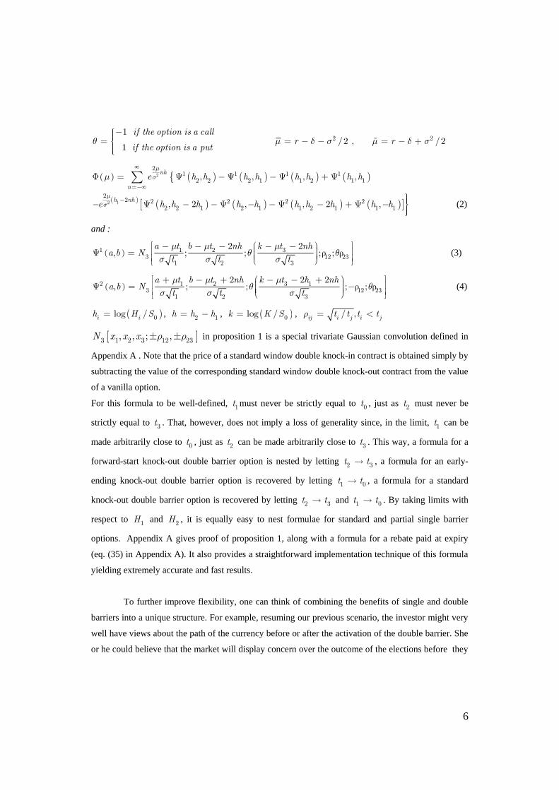
1

1 if the option is a call

if the option is a putq

2 2/2 , /2r rm d s m d s

2

21 1 1 1

2 2 2 1 1 2 1 1, , , ,nh

n

e h h h h h h h hm

sm

12

22 2 2 2 2

2 2 1 2 1 1 2 1 1 1, 2 , , 2 ,h nh

e h h h h h h h h h hm

s

(2)

and :

1 1 2 33 12 23

1 2 3

2 2,

a t b t nh k t nha b N

t t t

m m mq q

s s s

(3)

2 1 2 3 13 12 23

1 2 3

2 2 2,

a t b t nh k t h nha b N

t t t

m m mq q

s s s

(4)

0log /i ih H S , 2 1h h h , 0log /k K S , / ,ij i j i jt t t tr

3 1 2 3 12 23, , ; ,N x x x r r in proposition 1 is a special trivariate Gaussian convolution defined in

Appendix A . Note that the price of a standard window double knock-in contract is obtained simply by

subtracting the value of the corresponding standard window double knock-out contract from the value

of a vanilla option.

For this formula to be well-defined, 1t must never be strictly equal to 0t , just as 2t must never be

strictly equal to 3t . That, however, does not imply a loss of generality since, in the limit, 1t can be

made arbitrarily close to 0t , just as 2t can be made arbitrarily close to 3t . This way, a formula for a

forward-start knock-out double barrier option is nested by letting 2 3t t , a formula for an early-

ending knock-out double barrier option is recovered by letting 01t t , a formula for a standard

knock-out double barrier option is recovered by letting 2 3t t and 01t t . By taking limits with

respect to 1H and 2H , it is equally easy to nest formulae for standard and partial single barrier

options. Appendix A gives proof of proposition 1, along with a formula for a rebate paid at expiry

(eq. (35) in Appendix A). It also provides a straightforward implementation technique of this formula

yielding extremely accurate and fast results.

To further improve flexibility, one can think of combining the benefits of single and double

barriers into a unique structure. For example, resuming our previous scenario, the investor might very

well have views about the path of the currency before or after the activation of the double barrier. She

or he could believe that the market will display concern over the outcome of the elections before they

7

actually take place, putting the currency under strain. It would then be profitable to add a down-and-in

provision at that moment. She or he could also anticipate that the newly elected party will be the one

whose political and economic platform is the most likely to reassure market participants, which could

trigger a rally immediately after the vote. It would then be profitable to add an up-and-in provision at

that time. These additional features increase the chances of the option being activated. Besides, they

do not necessarily result in a more expensive premium since the investor could offset the cost of these

new opportunities by setting her or his double barrier further away from the underlying spot price.

In line with the usual terminology, these contracts could be called partial window double barrier

options since only part of the time interval during which barrier crossing is monitored contains a

double barrier, the rest of it containing single barriers. More specifically, let us divide the option life

as follows : 50 1 2 3 4 6 7t t t t t t t t , where 0t is the contract inception and 7t is the

contract expiry. If a single upper barrier is monitored within 1 2,t t , followed by a double barrier

within 3 4,t t and a single lower barrier within 5 6,t t , then one could speak of an up-and-down

partial window double barrier option. Similarly, when monitoring starts with a single upper barrier

within 1 2,t t , continues with a double barrier within 3 4,t t , and finishes with a single upper barrier

within 5 6,t t , then one could speak of an up-and-up type of contract. A third configuration is when

monitoring starts with a single lower barrier within 1 2,t t , continues with a double barrier within

3 4,t t , and finishes with a single upper barrier within 5 6,t t , which defines a down-and-up type of

contract. Finally, if a single lower barrier is monitored within 1 2,t t , followed by a double barrier

within 3 4,t t and a single lower barrier within 5 6,t t , then one could speak of a down-and-down

type of contract.

Note that monitoring of the double barrier may start immediately after monitoring the first single

barrier, i.e. one may have : 2 3t t . Likewise, there may be continuity in time between the

monitoring of the double barrier and that of the second single barrier ( 54t t ). Besides, there may of

course be only one single barrier, either before or after the double barrier. Given all these possible

specifications, as well as the choice between a knock-in and a knock-out provision and the choice

between a call and a put, there is a very large number of possible partial window double barrier

contracts. It is analytically feasible to obtain a unique closed form formula that can on its own provide

the exact value of all of them. This formula, including a possible rebate paid at expiry, is given in

appendix B, along with a simple numerical technique to implement it.

8

2. Numerical results

Let us now examine the behavior of prices for various contract specifications. Table 1

presents the values of standard window double knockout put options (SWDKOP) for several volatility

and barrier levels, and compares them with the values of standard double knockout puts (SDKOP) and

vanilla puts (VP). Three different SWDKOP prices are given : one applying the formula, one obtained

from a binomial tree, and one performing Monte Carlo simulation. Details on how these values were

obtained and how the different methods compare in terms of accuracy and efficiency can be found in

Appendix A.

In Table 1, the premium of a SWDKOP is, on average, 55.6% lower than that of a VP; for a SDKOP,

the premium discount amounts to 73.5%. Those figures point at the considerable savings investors can

expect from acquiring long positions in window-type options instead of vanilla options. They are also

in line with the fact that, by definition, the less valuable SDKOP contracts must be cheaper than the

SWDKOP ones. There are, however, three situations in which the premium of a SWDKOP and that of

a SDKOP tend to converge. The first one, quite obvious, is when double barrier monitoring extends

over the whole option life; but then, the SWDKOP contract loses its specificity and, in the limit,

cannot be distinguished from a SDKOP. The second one is when the distance between the upper and

the lower barrier is short, or when either the upper or the lower barrier is located very near the

underlying spot price, while volatility is high. Then, both the value of a SWDKOP and that of a

SDKOP rapidly drop and,in the limit, tend to zero, reflecting the overwhelming impact of the

likelihood of knocking-out, no matter how long the double barrier is monitored. When the double

barrier range is (80,120) and volatility is 44%, the value of a SWDKOP is thus only 1.6% of that of a

VP, the double barrier being active during one-third of the option life. The third configuration in

which the premium of a SWDKOP and that of a SDKOP tend to converge is when the distance

between the upper and the lower barrier is large and volatility is low. Then, the value of both a

SWDKOP and a SDKOP tends to that of a VP, reflecting the rapidly decreasing likelihood of

knocking-out.

Interestingly enough, there is a rather wide range of volatility, for each double barrier, in which

SWDKOP values do not differ significantly from one another. For instance, we see in Table 1 that,

with a double barrier set at (70,130), the SWDKOP value is quite the same whether volatility is 18%

or 25%. Likewise, when the double barrier is set at (60,140), the SWDKOP value is quite the same

whether volatility is 25% or 32%. The levels of volatility for which SWDKOP values do not differ

significantly among each other become lower as the upper barrier and the lower barrier get closer to

each other. Additional computations show that : the standard deviation of (80,120) SWDKOP prices is

9

0.046 when volatility ranges between 12% and 18% (for an average option value equal to 2.97), the

standard deviation of (70,130) SWDKOP prices is 0.038 when volatility ranges between 18% and

25% (for an average option value equal to 5.34), and the standard deviation of (60,140) SWDKOP

prices is 0.044 when volatility ranges between 25% and 32% (for an average option value equal to

8.07). This is because, in these volatility ranges, the chances of ending the option life in-the-money

and the risks of knocking-out before expiry offset each other in a balanced manner. This non-

monotonicity of the option value with respect to volatility can actually be observed, to a lesser or

greater extent, in all kinds of knock-out barrier options. This is one of their main differences with

vanilla options, which display non-linearity but monotonicity with respect to the volatility of the

underlying asset.

Let us now move on to partial window double knockout puts (PWDKOP). Tables 2 and 3

present the prices of up-and-down (UDP), down-and-up (DUP), up-and-up (UUP) and down-and-

down (DDP) partial window double knockout puts. They are an extension to the SWDKOP prices

presented in Table 1 in the sense that the same contract specifications have been kept except for a time

interval before and after the double barrier during which only the lower or the upper part of that

double barrier is monitored. This allows to compare PWDKOP and SWDKOP prices. The difference

between Table 2 and Table 3 lies in the extent of that time interval (long in Table 2, short in Table 3).

With these specifications, the UDP, DUP, UUP and DDP values in Tables 2 and 3 necessarily lie

between those of SDKOP (lower bound) and SWDKOP (upper bound) in Table 1. Again, Monte

Carlo simulation and binomial estimators are provided along with analytical values. Details on how

prices were obtained can be found in Appendix B.

By definition, since additional conditions are to be met, one would expect PWDKOP prices to be

lower than SWDKOP ones, especially in Table 2 where those additional conditions are imposed for a

longer period of time. Such an expectation is verified with UDP and DDP prices, but it is, to a

suprisingly large extent, hardly validated in the case of DUP and UUP prices. In Table 2, UDP prices

for instance are, on average, 51% lower than their SWDKOP counterparts, but DUP prices are only

4.2% lower than their SWDKOP counterparts. The closer the upper and the lower barrier to the spot

value, the more difference between PWDKOP and SWDKOP prices : in Table 2, the (80,120) UDP

premium is 78.9% lower than the corresponding (80,120) SWDKOP premium in Table 1, but the

(60,140) UDP premium is only 24.9% lower than that of the corresponding (60,140) SWDKOP; for

DUP options, the difference with SWDKOP prices is even almost negligible when the double barrier

is (70,130) or (60,140).

Another surprising feature of DUP and UUP prices is that they are almost the same when the single

barriers before and after the double barrier are monitored during a large (Table 2) or a short (Table 3)

10

time interval. The same phenomenon can be observed with up-and-down and down-and-down double

window call options. This is not true of UDP and DDP prices; UDP prices, for instance, exhibit a

substantial average difference of 32.1% between Table 2 and Table 3. Likewise, down-and-up and up-

and-up double window call option values differ significantly from one another according to the

amount of time during which single barriers are monitored, as one would expect intuitively. Actually,

this is simply because the likelihood of knocking-out as a function of time exposure to barrier

monitoring is more sensitive to the level of volatility in the case of UDP and DDP contracts : if

volatility is raised to 44%, then DUP and UUP prices also begin to exhibit large differences between

Table 2 and Table 3.

Finally, one last noticeable feature of both Tables 2 and 3 is the fact that UDP and DDP prices are

very similar, such as DUP and UUP prices, whatever the barrier levels.

3. Hedging issues

To eliminate risk, option dealers need to hedge their positions. Delta hedging, exploiting the

correlation between the option and its underlying, is the building block of dynamic hedging. The

gamma parameter measures by how much or how often a position must be rehedged in order to

maintain a delta-neutral position. Vega measures volatility risk exposure. The following discussion

briefly examines the delta, gamma and vega parameters of a number of window double knock-out

options. Analytical formulae for these hedge parameters can be derived by differentiation. However,

the derived formulae are cumbersome and it is easier and more efficient to look at finite-difference

approximations by measuring the sensitivity of the option value to a slight change in the appropriate

variable.

Let us compare the variations, with respect to the underlying asset price, of the hedge parameters of

two different standard window double knock-out call options, SWC1 and SWC2, and those of a

vanilla call, VC, as well as the variations, with respect to the underlying asset price too, of the hedge

parameters of two down-and-up partial window double knock-out call options, DUC1 and DUC2. For

all these options, the strike price is 100, volatility is 25%, the riskless rate is 5%, the dividend rate is

2%. The lower barrier and the upper barrier of both SWC1 and SWC2 are 70 and 130, respectively.

The SWC1 expiry is 1.5 years, with barrier monitoring within the time interval [0.5-1]. The SWC2

expiry is 0.3 years, with barrier monitoring within the time interval [0.1-0.2]. Such contract

specifications make it possible to gauge the effect of time to maturity on hedging. For DUC1 and

DUC2 options, the single lower and upper barriers are 70 and 130, respectively, and the (70,130)

double barrier is monitored within the time interval [0.5-1]. In the DUC1 case, the single lower barrier

11

is monitored within [0.2-0.3] and the single upper barrier is monitored within [1.2-1.3]. In the DUC2

case, the single lower barrier is monitored within [0-0.5] and the single upper barrier is monitored

within [1-1.5]. These contract specifications allow to compare partial window double knock-out and

standard window double knock-out hedge parameters, as well as to assess the impact of single barrier

monitoring before and after the double barrier.

First, SWC1 and SWC2 deltas are always smaller than or equal to VC deltas, whatever the underlying

spot value. This is because SWC1 and SWC2 options are cheaper than VC options, so that they stand

to gain or lose less value. Both SWC1 and SWC2 deltas are positive for out-of-the-money contract

specifications, even when the option is far out-of-the-money. But their value is small then, not only

because the probability of expiring in-the-money is low, but also because of the significant risk of

hitting the nearby lower barrier before expiry. Thus, the SWC1 delta is 9.5% at 71, which is less than

half of the corresponding VC delta.

In the region between 71 and 100, the SWC2 delta curve is remarkably close to the VC delta one,

increasing quite steeply from around zero to above 40% . In contrast, the SWC1 delta curve slowly

decreases, from 9.5% to around zero, as if the higher risk of hitting the upper barrier prevailed over

the higher chances of not hitting the lower barrier and expiring in-the-money. The region around 100

is interesting, since this is the area where the option is at-the-money and where the spot price is

equally distant from the lower and the upper barrier. Around this point, the SWC2 delta reaches its

peak (above 40%), and thus starts decreasing, while the SWC1 delta becomes negative. Beyond 100,

the SWC1 delta curve continues to decrease smoothly, while the SWC2 delta one rapidly falls down

to large negative values (around –50% near the upper barrier). This stands in complete opposition with

the behavior of a VC delta, which increases regularly as the option becomes more and more in-the-

money (because ending the option life in-the-money becomes more and more certain). This

divergence is caused by the upper barrier, which raises the risk of knocking-out when the option is in-

the-money. This effect is more pronounced when expiry is close (SWC2 case), leaving short time for

the underlying asset to drift away from the upper barrier.

Overall, delta variations are steeper and more unstable for SWC2 than for SWC1, reflecting the

significant impact of shorter time to maturity. As a result, SWC2 gamma values are larger than SWC1

gamma values : while the latter lie within a [0.6%, -0.8%] range, the former lie within a [3%, -5%]

range. This makes SWC2 options less easy to hedge than SWC1 options using a delta-neutral dynamic

strategy, since the hedging portfolio needs to be more frequently rebalanced. But when the barrier

period is sufficiently distant from the beginning and the end of the option life (SWC1 case), gamma

fluctuations are substantially smoother than with regular double knock-out barrier options, which is an

advantage for an option dealer.

12

If we now examine the vegas, computations reveal that most SWC1 and SWC2 vega values are

negative, unlike VC vega values, which are always positive whatever the underlying asset spot value.

This divergence is caused by the ambivalent effect of volatility on knock-out option values : higher

volatility increases the chances of expiring in-the-money, but also the risks of knocking-out. The

former effect prevails over the latter when the SWC2 option is out-of-the-money, with vega topping a

modest 2% when the underlying spot price is 90, but it goes reverse when the option is in-the-money.

Thus, SWC2 vega values become more and more negative as the underlying spot price gets closer to

the upper barrier ( -1% at 110,- 4.4% at 120, –10% at 128). When time to maturity is long (SWC1

case), however, vega values are at their highest levels when the option is far out-of-the-money (1.9%

at 71) or, to a lesser extent, when it is far in-the-money. This is because our contract specifications in

this example locate the double barrier right in the middle of the option life. Had monitoring of the

same barrier period (half a year) started soon after the beginning of the option life, vega values would

have reached a peak for out-of-the-money contracts; had it ended soon before the option expiry (one

year and a half), vega values would have been higher for far out-of-the-money contracts (with a peak

only slightly greater than zero, though). This complex vega behavior is a reminder of the significance

of time to maturity when it comes to measuring the impact of volatility on the risk of knocking-out.

Overall, vega parameters are all the more difficult to interpret as both SWC1 and SWC2 do not have

single-signed gamma everywhere. This leaves the option dealer quite exposed to volatility risk.

Next, one can turn to DUC1 and DUC2 hedge parameters. DUC2 prices are cheaper than

DUC1 ones, because more stringent conditions are imposed on DUC2 payoffs. Consequently, DUC2

deltas are smaller than their DUC1 counterparts, although this gap shrinks as the underlying asset spot

value approaches the upper knock-out barrier. Also, all DUC1 and DUC2 deltas remain positive,

which is a noticeable difference with SWC1 and SWC2 deltas. They attain a peak when the option is

slightly out-of-the-money (22% for DUC1 and 16% for DUC2 when the underlying spot price is 98).

Quite typically, they reach bottom in the regions near the knock-out barriers, especially the lower

barrier, which makes sense intuitively since it is the lower barrier that is first monitored (8.2% for

DUC1 and 1.4% for DUC2 when the underlying spot price is 71). Had we valued down-and-down or

up-and-up partial window double knock-out call options, however, we would have obtained a number

of negative deltas.

DUC1 and DUC2 gamma fluctuations are quite moderate, lying within [1.2%,-0.3%] and [1%,-0.6%]

ranges respectively. This is quite remarkable, especially in the DUC2 case where the whole option life

is subject to barrier monitoring. However, gamma fluctuations could obviously be larger for other

contract specifications, such as a shorter time to maturity or a narrower barrier range.

13

DUC1 and DUC2 vega values are quite similar. They are almost all negative, which is not surprising,

given the number of knock-out conditions. Less evident is the fact that DUC1 and DUC2 vegas hit

their lowest level when the option is slightly out-of-the-money (-5.2% at 99 for DUC1 and –3.5% at

98 for DUC2). Actually, this is simply because these are the regions where those options take their

highest value; likewise, the largest delta parameters can be obtained in these regions.

Overall, it should be kept in mind that there is potentially a number of contract specifications

for which dynamic hedging is either uneasy or relatively unreliable, due to gamma fluctuations and

because vegas do not always provide a clear measure of volatility risk. Theoretically, gamma risk

could be overcome by continuous rebalancing of the hedging portfolio, but, in practice, trading is

discrete and transaction costs can accumulate to substantial amounts. More seriously, like all kinds of

knock-out contracts, window double knock-out options are faced with a discontinuity of their delta at

the barrier (with gamma possibly reaching infinite values in finite time). The problem of hedging

close to the barrier is well described in Taleb (1997). As it is magnified near the option expiry, the

option dealer would be better off with a contract in which monitoring of the double barrier ends

sufficiently long before expiry. This is achievable with a window double knock-out contract, whereas

it is by definition impossible with a regular double (or single) knock-out contract. Hedging will be

made even easier if barrier monitoring starts sufficiently long after the beginning of the option life.

Compared with partial double knock-out contracts (whether forward-start or early-ending), window

double knock-out contracts allow to locate the double barrier away from both the beginning and the

end of the option life. Thus, window double knock-out options do not eliminate hedging problems, but

they can alleviate them, compared with other forms of double knock-out contracts.

The potential difficulties associated with dynamic hedging seem to call for a static hedging strategy

(Carr, Ellis and Gupta, 1998) although this often merely shifts the problem to the vanilla options

market, as static hedges need to be rebalanced too when the underlying spot value nears the knock-out

barrier (Toft and Xuan, 1998). An interesting alternative is the superhedging strategy (Schmock,

Shreve and Wystup, 1999; Wystup, 1999), which achieves continuity at the barrier by numerically

solving a stochastic control problem under a constraint on the possible values of the gearing ratio of

the option. This approach works well with regular double knock-out contracts. It could be extended to

window double knock-out contracts.

4. Concluding remarks

This paper has studied standard and partial window double barrier options. These contracts

are more flexible than regular double barrier ones, thus allowing to match more closely the hedging

14

needs or the speculative views of investors. As few as two formulae suffice to cover a very large

number of complex payoffs. They are the basis for simple numerical integration schemes which

compare favourably with alternative pricing approaches in terms of accuracy and efficiency. They also

provide an easy and reliable way to obtain finite-difference approximations to hedge parameters.

Barriers have been assumed constant in this paper, but it would be an easy extension to make them

deterministic exponential functions of time. Stochastic volatility and interest rates, however, would

not be an easy extension, and there is no evidence that such a valuation problem would be analytically

tractable.

Appendix A : proof and numerical implementation of the valuation formula for

a standard window double barrier option

In this appendix, the following notations will be used :

- tW is Brownian motion defined on a probability space , ,tF P where ,stF W s ts is the

natural filtration of tW

- tS is the value of the underlying asset at time t

- K is the strike price, 1H is the lower barrier, 2H is the upper barrier, r is the instantaneous riskless

rate, s is the constant volatility of the underlying asset, d is the constant continuous dividend rate

- 0ln /t tX S S , 0ln /k K S , 0ln /i ih H S ,

,

infa b

ba t

t t tm X

,

,sup

a b

ba t

t t tM X

-Q is the risk-neutral measure, .QE is the expectation operator under the Q measure

- .1 is the indicator function taking value 1 if the conditions inside the brackets are met and value

zero otherwise

- .N refers to the univariate standard normal cumulative distribution function, ;2 .,.N r refers to

the bivariate standard normal cumulative distribution function with correlation coefficient r

A.1 The multivariate normal distribution

In general, if 1,..., nX X X is a vector of n joint standardized normal random variables with a

symmetric, positive-definite n n matrix of variances and covariances , then the density of X is

given by :

15

1

2

1 /2,...,

2

TX X

n n

ef x x

Detp

(5)

where TX is the transpose of X , Det is the determinant of and 1 is the inverse of (for a

proof, see e.g., Tong, 1990).

For example, if we denote by 12 23, and 13r the correlation coefficients between three standardized

normal random variables 1 2,X X and 3X , it is easily shown, by applying formula (5), that the joint

density f of 1 2,X X and 3X is given by :

2 2 251 2 3 4 6

12 2 2

2

12 23 13 3/2( , , ; , , )

2

a b c ab bc ace

f a b cDet

l l l l l l

rp

(6)

with : Det 2 2 212 23 13 12 23 131 2r r r

2 2 223 13 12 13 23 12

1 2 3 4

1 1 1;

Det Det Det Det

r r r rl l l l

13 12 23 12 23 13

5 6Det Det

r rl l

However, using these general multinormal expressions becomes analytically cumbersome and

computationally inefficient as the dimension of the integral rises. Actually, simplified expressions can

be used when dealing with the finite-dimensional distributions of geometric Brownian motion GBM.

Let 1t , 2t , 3t be three different dates during the option life 0 3,t t , such that : 0 1 2 3t t t t . By

conditioning with respect to2t

X and applying the Markov property of Brownian motion, we have :

1 2 3

, ,t t tQ X a X b X c

1 21 2 3

,,

t t t

Q Qt tX a X b X c

E E X a X b

1 1 (7)

21 2 3

,t t t

Q QtX a X b X c

E E X b

1 1 (8)

21 2

1 2

3

21 2

1 2

1 2

2 /

2 1 /

2 1 / t

a t b t

t t

Q

X c

t t

t t

x xy y

eE y dydx

t t

m m

s s

p

1 (9)

21 2

1 2

21 2

1 2 3 2

3 21 2

2 /

2 1 /

2 1 /

a t b t

t t

t t

t t

x xy y

c y t teN dydx

t tt t

m m

s sm

sp

(10)

16

1 2 3 1 2 2 3

1 2 31 2 2 3

2 22 / /

3/21 2 2 3

2 1 / 2 1 /2

2 1 / 1 /

a t b t c t t t t

t t t

t

t t t t

y x z yx

edzdydx

t t t t

m m m

s s s

p

(11)

where 2 /2rm d s

This can be written in a more compact form as :

1 2 33 12 23

1 2 3

, , ,a t b t c t

Nt t t

m m m

s s s

(12)

where 12 1 2/t tr and 23 2 3/t t

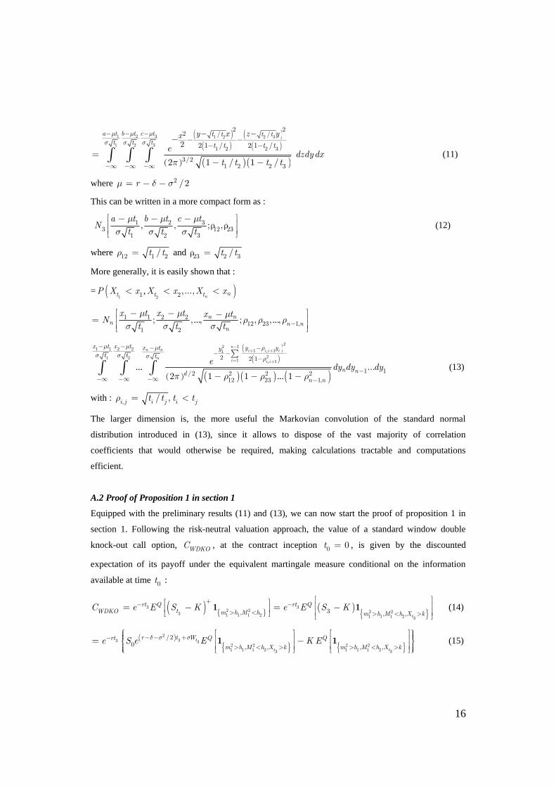
More generally, it is easily shown that :

= ,1 21 2,..., n

nt t tP X x X x X x

... ...1 1 2 212 23 1,

1 2

, , , , ,n nn n n

n

x t x t x tN

t t t

m m mr r r

s s s

212

1 2 1 , 112, 1

......

1 2

1 212 2 1

1 1/2 2 2 212 23 1,

...2 1 1 1

nn n ii i i

ni i i

x t x t x t y yyt t t

n ndn n

edy dy dy

m m m rs s s r

p r r r

(13)

with : , / ,i j i j i jt t t tr

The larger dimension is, the more useful the Markovian convolution of the standard normal

distribution introduced in (13), since it allows to dispose of the vast majority of correlation

coefficients that would otherwise be required, making calculations tractable and computations

efficient.

A.2 Proof of Proposition 1 in section 1

Equipped with the preliminary results (11) and (13), we can now start the proof of proposition 1 in

section 1. Following the risk-neutral valuation approach, the value of a standard window double

knock-out call option,WDKOC , at the contract inception 0 0t , is given by the discounted

expectation of its payoff under the equivalent martingale measure conditional on the information

available at time 0t :

3 3

2 2 2 23 1 1 1 2 1 1 1 2 3

3, , , t

rt Q rt QtWDKO m h M h m h M h X k

C e E S K e E S K

1 1 (14)

2

33 32 2 2 21 1 1 2 1 1 1 23 3

/20 , , , ,

t

t t

r t Wrt Q Q

m h M h X k m h M h X ke S e E K Ed s s

1 1 (15)

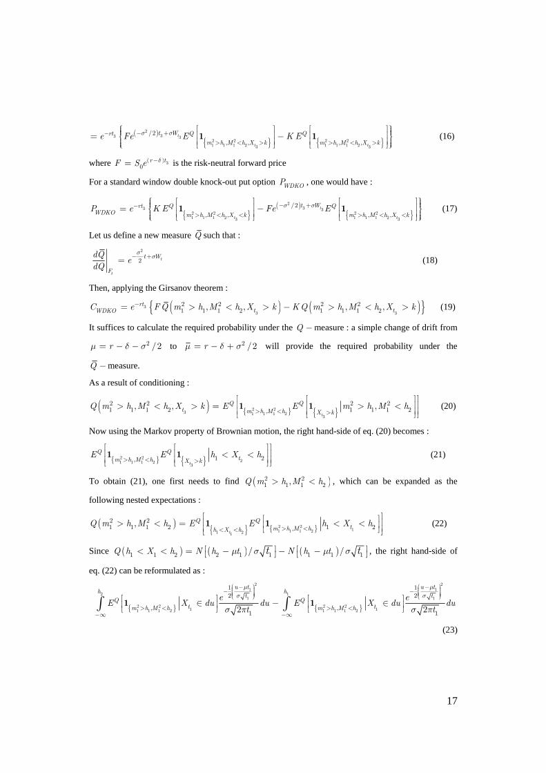
17

2

33 32 2 2 21 1 1 2 1 1 1 23 3

/2

, , , ,t

t t

t Wrt Q Q

m h M h X k m h M h X ke Fe E K Es s

1 1 (16)

where 3

0r tF S e d is the risk-neutral forward price

For a standard window double knock-out put option WDKOP , one would have :

2

33 32 2 2 21 1 1 2 1 1 1 23 3

/2

, , , ,t

t t

t Wrt Q QWDKO m h M h X k m h M h X k

P e K E Fe Es s

1 1 (17)

Let us define a new measure Q such that :

2

2 t

t

t W

F

dQe

dQ

ss

(18)

Then, applying the Girsanov theorem :

3

3 3

2 2 2 21 1 1 2 1 1 1 2, , , ,rt

t tWDKOC e FQ m h M h X k KQ m h M h X k (19)

It suffices to calculate the required probability under the Q measure : a simple change of drift from

2 /2rm d s to 2 /2rm d s will provide the required probability under the

Q measure.

As a result of conditioning :

2 23 1 1 1 2

3

2 2 2 21 1 1 2 1 1 1 2,

, , ,t

Q Qt m h M h X k

Q m h M h X k E E m h M h1 1 (20)

Now using the Markov property of Brownian motion, the right hand-side of eq. (20) becomes :

2 221 1 1 2

3

1 2,t

Q Qtm h M h X k

E E h X h

1 1 (21)

To obtain (21), one first needs to find 2 21 1 1 2,Q m h M h , which can be expanded as the

following nested expectations :

2 2

11 1 1 21 21

2 21 1 1 2 1 2,

,t

Q Qtm h M hh X h

Q m h M h E E h X h

1 1 (22)

Since 1 1 2 2 1 1 1 1 1/ /Q h X h N h t N h tt tm s m s , the right hand-side of

eq. (22) can be reformulated as :

2 21 1

2 11 1

2 2 2 21 11 1 1 2 1 1 1 2

1 1

2 2

, ,1 12 2

u t u th h

t tQ Q

t tm h M h m h M h

e eE X du du E X du du

t t

m m

s s

s p s p

1 1

(23)

18

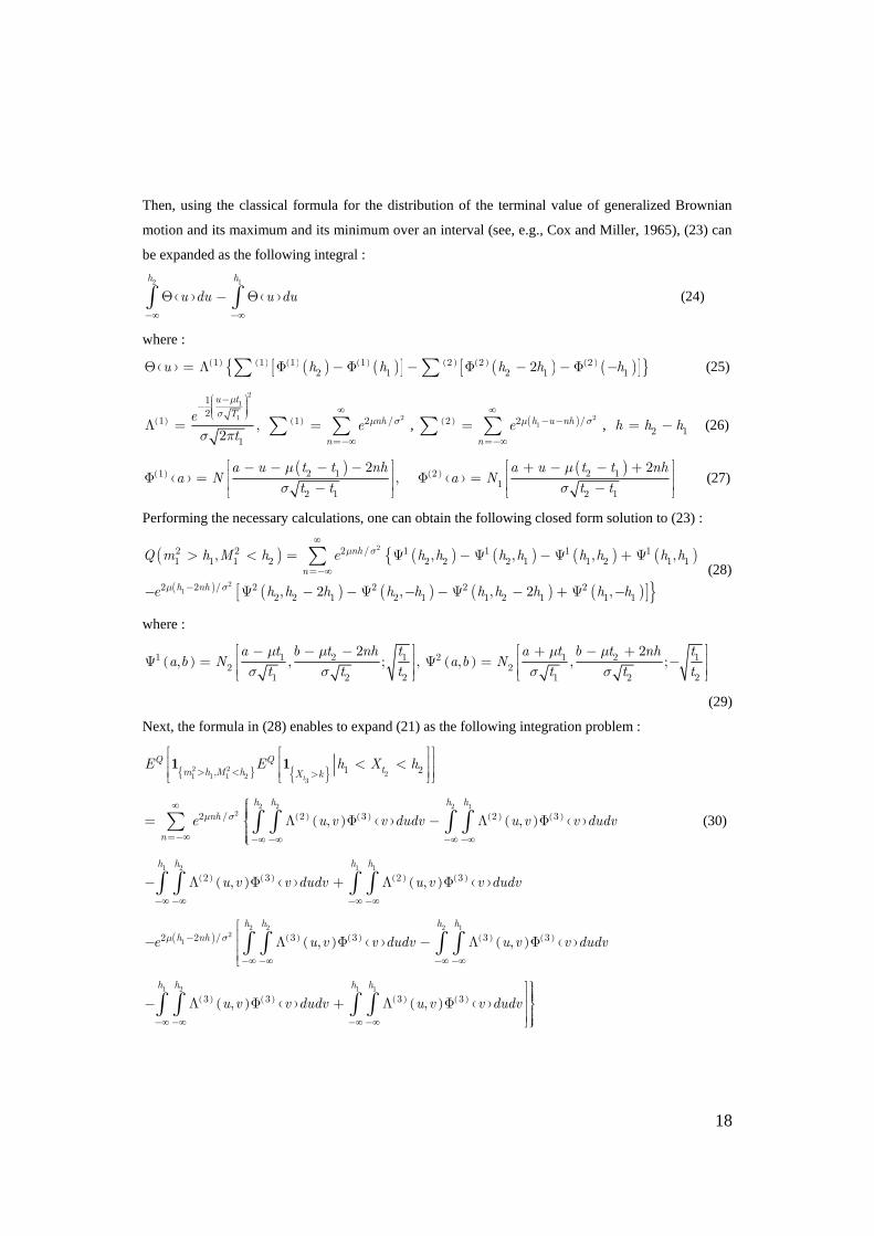
Then, using the classical formula for the distribution of the terminal value of generalized Brownian

motion and its maximum and its minimum over an interval (see, e.g., Cox and Miller, 1965), (23) can

be expanded as the following integral :

2 1h h

u du u du

(24)

where :

1 1 1 1 2 2 2

2 1 2 1 12u h h h h h (25)

21

1

1

21

1

,2

u t

Te

t

m

s

s p

21 2 /nh

n

e m s

,

212 2 /h u nh

n

e m s

, 2 1h h h (26)

2 1 2 11 21

2 1 2 1

2 2,

a u t t nh a u t t nha N a N

t t t t

m m

s s

(27)

Performing the necessary calculations, one can obtain the following closed form solution to (23) :

2

21

2 2 2 / 1 1 1 11 1 1 2 2 2 2 1 1 2 1 1

2 2 / 2 2 2 22 2 1 2 1 1 2 1 1 1

, , , , ,

, 2 , , 2 ,

nh

n

h nh

Q m h M h e h h h h h h h h

e h h h h h h h h h h

m s

m s

(28)

where :

1 1 2 1 2 1 2 12 2

2 21 2 1 2

2 2, , , , ,

a t b t nh t a t b t nh ta b N a b N

t tt t t t

m m m m

s s s s

(29)

Next, the formula in (28) enables to expand (21) as the following integration problem :

2 221 1 1 2

3

1 2,t

Q Qtm h M h X k

E E h X h

1 1

2 2 2 122 / 2 3 2 3, ,

h h h h

nh

n

e u v v dudv u v v dudvm s

(30)

1 2 1 1

2 3 2 3, ,

h h h h

u v v dudv u v v dudv

2 2 2 12

12 2 / 3 3 3 3, ,

h h h h

h nhe u v v dudv u v v dudvm s

1 2 1 1

3 3 3 3, ,

h h h h

u v v dudv u v v dudv

19

where :

22

2 11

1 2 1

21

22

21 2 1

,2 ( )

v u t t nhu t

t t teu v

t t t

mm

s s

ps

(31)

22

1 2 11

1 2 1

2 21

23

21 2 1

,2 ( )

v u h t t nhu t

t t teu v

t t t

mm

s s

ps

(32)

3 23

3 2

k v t tv N

t t

m

s

(33)

For a standard window double knock-out put option, the function

3 v would be :

3 23

3 2

k v t tv N

t t

m

s

(34)

A closed form solution can be found to the integration problem (30), which is precisely the formula

for a standard window double knock-out option given in Proposition 1, section 1.

As mentioned in section 1, a rebate provision may be included in the contract, giving the option holder

the right to receive an amount R at expiry if the option has been knocked-out. The value, RV , of the

standard window double knock-out option then becomes :

3 2 21 1 1 21 ,R rtV V e R Q m h M h (35)

where V is the option value without rebate as given by Proposition 1 in section 1, and

2 21 1 1 2,Q m h M h is explicitly given by eq. (14) in this Appendix.

A.3 Numerical implementation of Proposition 1 in section 1

The trivariate normal integrals appearing in Proposition 1 of section 1, defined by eq. (11) in this

appendix, must be numerically integrated. Several algorithms have already been designed to compute

trivariate normal cumulative distribution functions (Genz, 2001). However, they do not fit the specific

convolution used in (11). The following simple rule can be used instead :

2 /2 12 23

3 12 23 2 212 23

1, , ,

2 1 1

b

x a x c xN a b c e N N dx

r r

p r r

(36)

This numerical integration is very easy to perform. A level of at least 610 accuracy, which is more

than enough for option pricing, can be achieved with a mere 16-point Gauss-Legendre rule (and a

lower bound of – 8.5 in the integral). Moreover, the integration rule in (36) is extremely efficient : the

analytical values reported in Table 1 take a computational time of 0.4 second for the eight out of

20

twelve prices requiring the computation of three terms in the infinite series, and and average 0.6

second for the others (on a modest 2.4 Ghz-clock PC). Note that, at most, nine terms in the infinite

series were required. In general, more and more terms are needed as the lower barrier and the upper

barrier are closer to one another and as volatility increases. But, in the vast majority of cases, very few

leading terms are required. Only for unrealistic contract specifications may significant errors arise

from the truncation of the infinite series. This is in line with the findings of Kunitomo and Ikeda

(1992) regarding standard double barrier options.

Along with analytical values, Table 1 reports numerical results obtained by binomial and Monte Carlo

simulation methods. The binomial estimates are computed with 500 timesteps. The jump and

probability parameters are set according to the Trigeorgis approach (1992), which has been proved to

be slightly more accurate than that of Cox, Ross and Rubinstein (1979) or that of Jarrow and Rudd

(1983). In addition, the lattice is constructed in such a way that there are horizontal layers of nodes as

close as possible to the upper barrier and to the lower barrier, following the recommendations of

Boyle and Lau (1994). Prices are obtained in less than one second. The binomial estimates diverge

from the exact prices by 0.58% on average.

The Monte Carlo simulation estimates were obtained after running 1,000,000 simulations per option

value and implementing a computationally demanding discretization of 16 monitoring times per

business day for the time segment in which the double barrier is active. The efficiency of such a

procedure is obviously very poor and definitely not suited to real time trading environments.

Appendix B : Valuation of partial window double barrier options

B.1 Analytical formula

Proposition 2 :

The value V of a partial window double knock-out option is given by :

dd s q m m 7 7

50 01 2 3 4 1 2 3 4 6 7, , , , , , , , , , , , , , , rt tPWDKOV S K H H H H r t t t t t t t e K e S

(37)

where :

0S is the underlying asset spot value, K is the strike price, r is the constant instantaneous riskless

rate, s is the underlying asset’s constant volatility, d is its constant continuous dividend rate;

2H is the lower part of the double barrier, 3H is the upper part of the double barrier;

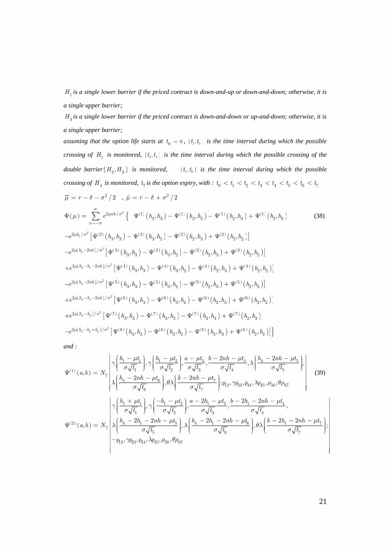
21

1H is a single lower barrier if the priced contract is down-and-up or down-and-down; otherwise, it is

a single upper barrier;

4H is a single lower barrier if the priced contract is down-and-down or up-and-down; otherwise, it is

a single upper barrier;

assuming that the option life starts at 0 0t , 1 2,t t is the time interval during which the possible

crossing of 1H is monitored, 3 4,t t is the time interval during which the possible crossing of the

double barrier 2 3,H H is monitored, 5 6,t t is the time interval during which the possible

crossing of 4H is monitored, 7t is the option expiry, with : 50 1 2 3 4 6 7t t t t t t t t

2 /2rm d s , 2 /2rm d s

m sm

22 /nh

n

e 1 1 1 13 3 3 2 2 3 2 2, , , ,h h h h h h h h (38)

m s 2

12 / 2 2 2 23 3 3 2 2 3 2 2, , , ,he h h h h h h h h

m s 2

22 2 / 3 3 3 33 3 3 2 2 3 2 2, , , ,h nhe h h h h h h h h

m s 2

2 12 2 / 4 4 4 43 3 3 2 2 3 2 2, , , ,h h nhe h h h h h h h h

m s 2

42 2 / 5 5 5 53 3 3 2 2 3 2 2, , , ,h nhe h h h h h h h h

m s 2

4 12 2 / 6 6 6 63 3 3 2 2 3 2 2, , , ,h h nhe h h h h h h h h

m s 2

4 22 / 7 7 7 73 3 3 2 2 3 2 2, , , ,h he h h h h h h h h

m s 2

4 2 12 / 8 8 8 83 3 3 2 2 3 2 2, , , ,h h he h h h h h h h h

and :

m m m m mg g l

s s s s s

mml ql g l r qr

s s

51 1 1 2 3 4 4

51 2 3 417

74 612 23 34 45 56 67

6 7

2 2, , , , ,

,22

, , , , , ,

h t h t a t b nh t h nh t

t t t t ta b N

k nh th nh t

t t

(39)

m m m mg g

s s s s

mm ml l ql

s s s

g l r

1 1 1 2 1 3 1 4

1 2 3 4

5 1 72 4 1 4 1 67

5 6 7

12 23 34 45 56

2 2 2, , , ,

2 22 2 2 2, , ,

, , , , ,

h t h t a h t b h nh t

t t t t

k h nh th h nh t h h nh ta b N

t t t

qr

67

22

m m m m mg g l

s s s s s

mml ql g l r qr

s s

51 1 1 2 3 2 4 4 2

51 2 3 437

2 74 2 612 23 34 45 56 67

6 7

2 2 2 2, , , , ,

,2 22 2

, , , , , ,

h t h t a t b h nh t h h nh t

t t t t ta b N

k h nh th h nh t

t t

m m m mg g

s s s s

m ml l

s s

mql g

s

1 1 1 2 1 3 2 1 4

1 2 3 4

54 4 2 1 4 2 1 67

5 6

2 1 712

7

2 2 2 2, , , ,

2 2 2 2 2 2, , ,

2 2 2,

h t h t a h t b h h nh t

t t t t

h h h nh t h h h nh ta b N

t t

k h h nh t

tl r qr

23 34 45 56 67, , , ,

m m m m mg g l

s s s s s

mml ql g l r qr

s s

51 1 1 2 3 4 4

51 2 3 457

4 74 612 23 34 45 56 67

6 7

2 2, , , , ,

,2 22

, , , , , ,

h t h t a t b nh t h nh t

t t t t ta b N

k h nh th nh t

t t

m m m mg g

s s s s

m ml l

s s

mql g l

s

1 1 1 2 1 3 1 4

1 2 3 4

56 4 1 4 1 67

5 6

4 1 712 23 34 45

7

2 2 2, , , ,

2 2 2 2, , ,

2 2 2, , ,

h t h t a h t b h nh t

t t t t

h h nh t h h nh ta b N

t t

k h h nh t

tr qr

56 67, ,

m m m m mg g l

s s s s s

mml ql

s s

g l r

51 1 1 2 3 2 4 4 2

51 2 3 4

4 2 77 4 2 67

6 7

12 23 34 45 56

2 2 2 2, , , , ,

2 2 22 2, ,

, , , ,

h t h t a t b h nh t h h nh t

t t t t t

k h h nh th h nh ta b N

t t

qr

67,

m m m mg g

s s s s

m ml l

s s

mql

s

1 1 1 2 1 3 2 1 4

1 2 3 4

58 4 2 1 4 2 1 67

5 6

4 2 1 7

7

2 2 2 2, , , ,

2 2 2 2 2 2, , ,

2 2 2 2

h t h t a h t b h h nh t

t t t t

h h h nh t h h h nh ta b N

t t

k h h h nh t

tg l r qr

12 23 34 45 56 67, , , , ,

r 0 03 2log / , , log / , /i i ij i jh H S h h h k K S t t , i jt t

1

1g

if the option is a down - and - up call or put or a down - and - down call or put

otherwise

23

1

1

if the option is an up - and - down call or put or a down - and - down call or put

otherwisel

1

1

if the option is an up - and - down put or an up - and - up call

or a down - and - up call or a down - and - down put

otherwise

q

This formula may appear cumbersome at first glance. Yet, it can rightfully be regarded as

particularly concise in view of the very large variety of complex contracts it enables to value.

57 1 2 3 4 6 7 12 23 34 45 56 67, , , , , , , , , , ,N x x x x x x x is a special form of the normal

cumulative distribution function, defined by eq. (13) in Appendix A. Note that the price of a partial

window double knock-in option is obtained simply by subtracting the value of the corresponding

partial window double knock-out option from the price of a vanilla option.

For proposition 2 to be well-defined, any it must never be strictly equal to jt , where i j .

This, however, does not imply a loss of generality since, in the limit, it can be made arbitrarily close

to jt . This is how we use proposition 2 to obtain the analytical values reported in Table 2, section 2 :

we let 01 ,t t 3 2,t t 5 4t t and 7 6t t . More specifically, we take the following

approximations of continuity: 1 0.0001t , 2 0.4999t , 5 1.0001t and 6 1.4999t , recalling

that 0 0t , 3 0.5t , 4 1t and 7 1.5t . Further refinement of these approximations is

numerically insignificant.

As mentioned in section 1, a rebate provision may be included in the contract, giving the option holder

the right to receive an amount R at expiry if the option has been knocked-out. The value, RV , of the

partial window double knock-out option then becomes :

7 2 4 4 651 1 3 2 3 3 41 , , ,R rtV V e R Q M h m h M h m h (40)

if the option is up-and-down

7 2 4 4 651 1 3 2 3 3 41 , , ,R rtV V e R Q m h m h M h M h (41)

if the option is down-and-up

7 2 4 4 651 1 3 2 3 3 41 , , ,R rtV V e R Q M h m h M h M h (42)

if the option is up-and-up

7 2 4 4 651 1 3 2 3 3 41 , , ,R rtV V e R Q m h m h M h m h (43)

if the option is down-and-down

24

where V is the option value without rebate, and where we recall that .Q is the probability operator

under the equivalent martingale measure, under which : 2 /2rm d s . The probabilities

involved in (40)-(43), which correspond to digital partial window double barrier options, are deduced

from Proposition 2 above by taking the first six dimensions of each , 1,..., 8i i in m , all

other things being equal .

B.2 Sketch of proof

Using the same notations and following the same first steps as with standard window double

knock-out options (Appendix A), the no-arbitrage value of an up-and-down partial window double

knock-out call can be expressed as :

7

7

7

2 4 4 651 1 3 2 3 3 4

2 4 4 651 1 3 2 3 3 4

, , , ,

, , , ,

trtPWUD

t

FQ M h m h M h m h X kC e

KQ M h m h M h m h X k

(44)

Similarly, the no-arbitrage value of a down-and-up partial window double knock-out call can be

expressed as :

7

7

7

2 4 4 651 1 3 2 3 3 4

2 4 4 651 1 3 2 3 3 4

, , , ,

, , , ,

trtPWDU

t

FQ m h m h M h M h X kC e

KQ m h m h M h M h X k

(45)

The no-arbitrage value of an up-and-up partial window double knock-out call can be expressed as :

7

7

7

2 4 4 651 1 3 2 3 3 4

2 4 4 651 1 3 2 3 3 4

, , , ,

, , , ,

trtPWUU

t

FQ M h m h M h M h X kC e

KQ M h m h M h M h X k

(46)

Finally, the value of a down-and-down partial window double knock-out call can be expressed as :

7

7

7

2 4 4 651 1 3 2 3 3 4

2 4 4 651 1 3 2 3 3 4

, , , ,

, , , ,

trtPWDD

t

FQ m h m h M h m h X kC e

KQ m h m h M h m h X k

(47)

where Q is a measure such that :2

2 t

t

t W

F

dQe

dQ

ss

. Multiplying by 1 and substituting

“ 7t

X k ” with “ 7t

X k ” in (44)-(47) provides the corresponding put option expressions.

Obtaining these probabilities involves long calculations that cannot be reproduced here. We simply

outline how it works in the case of an up-and-down partial window double knock-out call option,

knowing that the method is the same as with standard window double knock-out options (for which a

25

detailed proof is given in Appendix A). Basically, it boils down to repeatedly conditioning and

making use of the Markov property of Brownian motion. Thus, the first stage is to calculate :

2

11 111

21 1

t

Q QtM hX h

Q M h E E X1 1 (48)

This result is then used to find :

23 21 1 1 2 32 3

21 1 2 3 1,

,t t

Q Qt tM h X h h X h

Q M h h X h E E X h1 1 (49)

The next probability to calculate is :

4 42 33 2 3 31 1 2 33

2 4 41 1 3 2 3 3 2 3,,

, ,t

Q Qtm h M hM h h X h

Q M h m h M h E E h X h

1 1

(50)

Conditioning goes on until the last stage where the final probability to work out is :

7

2 4 4 651 1 3 2 3 3 4, , , , tQ M h m h M h m h X k

2 6 651 1 2 3 3 4 46 7

4, , , t t

Q QtM h h X h m h X h X k

E E X h

1 1 (51)

At each stage, each new conditional expectation can be written as a sum of multiple integrals of

increasing dimension. Appropriate changes of variables and simplifications allow to reduce those

multiple integrals to the convolutions of the standard normal distribution functions provided in

Appendix A.

B.3 Numerical implementation

Proposition 2 in this Appendix consists of a sum of seven-dimensional integrals. In this case, there is

no simple dimension reduction trick to get down to a one-dimensional integral similar to the one we

used in Appendix A. However, the special convolution of the multivariate standard normal

distribution introduced in eq. (4) of Appendix A allows to apply the following straightforward Monte

Carlo integration algorithm :

(i) To compute 7 1 2 7 12 23 67, ,..., , ,...,N x x x r r r , first draw n samples of seven uniform

numbers 0,1 , 1,..., 7 , 1,...,jiu i j n and turn them into n samples of seven

independent normal deviates , 1,..., 7 , 1,...,jiy i j n with zero mean and unit variance

1 20,1 , 0,1 ,...,j jy N y N 7 0,1jy N , using, e.g., the polar rejection algorithm (Press et

al., 1992)

26

(ii) Next, turn these n samples of seven independent normal deviates into n samples of seven

correlated normal deviates :

2 2 21 12 1 12 2 23 2 23 3 67 6 67 7, 1 , 1 ,..., 1j j j j j j jy y y y y y yr r r r r r , 1,...,j n

(iii) Then, test the relevant conditions for each deviate in each sample :

2 21 1 12 1 12 2 2 67 6 67 7 7, 1 , ..., 1j j j j jy x y y x y y xr r r r , 1,...,j n

If we denote by M the number of samples having passed the previous test, then the cumulative

distribution function 7 1 2 7 12 23 67, ,..., , ,...,N x x x r r r can be approximated by /M n . By the strong

law of large numbers, this sampling rule tends to the exact value of 7 1 2 7 12 23 67, ,..., , ,...,N x x x r r r

as n goes to infinity. Note that this algorithm is readily extended to higher-dimensional cumulative

distribution functions, as its convergence rate is independent of dimension.

In practice, the speed of convergence largely relies on the way the uniform deviates

, 1,..., 7 , 1,...,jiu i j n are drawn at stage (i) of the algorithm. Pseudo-random numbers can be

used, along with classical variance reduction techniques such as antithetic variates, stratified or Latin

hypercube sampling. However, convergence is achieved much faster by using quasi random numbers

instead of pseudo random numbers, thanks to the greater uniformity of low discrepancy sequences

(Niederreiter, 1992). To obtain the analytical values reported in Tables 2 and 3 in section 2, seven

different sequences of 20,000 Sobol points (Sobol, 1967) have been used, applying the code provided

by Press et al. (1992). This leads to computational times of 2.4 seconds for the 20 out of 24 option

prices that require the computation of three terms in the infinite series, and 3.2 seconds for the others

(that require five terms in the infinite series). The binomial and Monte Carlo simulation estimates

provided in Tables 2 and 3 in section 2 are obtained in the same way as in Appendix A. Again,

binomial results are excellent in terms of efficiency, with computational time as low as 0.8 second to

obtain an option price (recalling that 500 timesteps are used). However, one should not jump to the

conclusion that the binomial method is more efficient than the analytical one combined with Monte

Carlo quasi-random sampling. First, for options written with a longer time-to-maturity than that used

in Tables 2 and 3 (1.5 year), more timesteps would be required. More importantly, to assess the

overall efficiency of a numerical technique, it is necessary to take into consideration the time needed

to implement it in the first place, as well as the time that may be required to adapt it to future valuation

problems. In that respect, once you have typed the formula given by Proposition 2, your job is done,

with no need for subsequent trimming of your code, whatever the contract specifications or the model

inputs. The same is not true with trees, which can lead to significant errors when applied to complex

27

path-dependent payoffs such as those of partial window double barrier options. Consequently, trees

will have to be modified as new valuation problems arise.

Tables

Table 1. Comparison between standard window double knockout put prices (SWDKOP), standard

double knockout put prices (SDKOP) and vanilla put prices (VP) a

Lower /

Upper

barrier

Volatility SWDKOP

(analytical)

SWDKOP

(binomial)

SWDKOP

(simulation)

SDKOP

(analytical)

VP

(analytical)

80/120 18 % 2.83 2.84 2.85 1.15 6.37

25 % 1.94 1.93 1.96 0.32 9.54

32 % 1.12 1.13 1.15 0.05 12.71

44 % 0.30 0.30 0.31 0 18.09

70/130 18 % 5.26 5.26 5.28 3.88 6.37

25 % 5.19 5.20 5.23 2.56 9.54

32 % 4.22 4.21 4.22 1.24 12.71

44 % 2.40 2.40 2.44 0.21 18.09

60/140 18 % 6.23 6.23 6.25 5.76 6.37

25 % 7.97 7.98 7.98 5.91 9.54

32 % 7.97 7.97 7.99 4.45 12.71

44 % 6.16 6.14 6.19 1.83 18.09

a This table presents the prices of standard window double knockout put options (SWDKOP), standard

double knockout put options (SDKOP) and vanilla put options (VP) for four different levels of

volatility. All contracts are at-the-money with strike price 100. The option life, measured in years, is

[0-1.5]. The window double barrier is monitored within [0.5-1]. The standard double barrier, by

definition, is monitored within [0-1.5].The riskless rate is 5%, the dividend rate is 2%. There are no

rebate provisions. SWDKOP analytical values were obtained applying the formula given in

Proposition 1, section 1, by means of the implementation rule given in Appendix A, § 3. Binomial and

Monte Carlo simulation estimates were obtained using the techniques described in Appendix A, § 3.

SDKOP and VP analytical values were obtained using standard formulae (see, e.g., Zhang, 1998).

28

Table 2 . Comparison between up-and-down partial (UDP), down-and-up (DUP), up-and-up (UUP)

and down-and-down (DDP) window double knockout put prices a

Lower /

Upper barrier

analytical binomial simulation

80/120 UDP 0.42 0.41 0.43

70/130 UDP 2.63 2.62 2.66

60/140 UDP 5.95 5.96 5.97

80/120 DUP 1.70 1.72 1.71

70/130 DUP 5.11 5.12 5.15

60/140 DUP 7.94 7.96 7.96

80/120 UUP 1.62 1.63 1.61

70/130 UUP 5.03 5.04 5.08

60/140 UUP 7.92 7.92 7.88

80/120 DDP 0.44 0.44 0.46

70/130 DDP 2.68 2.70 2.70

60/140 DDP 5.27 5.29 5.27

a This table presents the prices of up-and-down (UDP), down-and-up (DUP), up-and-up (UUP) and

down-and-down (DDP) partial window double knockout put options for three different levels of the

lower and upper barriers. All contracts are at-the-money with strike price 100. The option life,

measured in years, is [0-1.5]. The window double barrier is monitored within [0.5-1]. The first single

barrier is monitored within [0-0.5] and the second single barrier is monitored within [1-1.5]. Volatility

is equal to 25%. The riskless rate is 5%, the dividend rate is 2%. There are no rebate provisions.

Analytical prices were obtained applying the formula given by Proposition 2 in Appendix B, § 1, by

means of the implementation rule given in Appendix B, § 3. Binomial and Monte Carlo simulation

estimates were obtained using the techniques described in Appendix A, § 3.

29

Table 3 . Comparison between up-and-down partial (UDP), down-and-up (DUP), up-and-up (UUP)

and down-and-down (DDP) window double knockout put prices a

Lower /

Upper barrier

analytical binomial simulation

80/120 UDP 0.91 0.93 0.95

70/130 UDP 3.72 3.73 3.75

60/140 UDP 6.97 6.97 6.95

80/120 DUP 1.81 1.82 1.84

70/130 DUP 5.16 5.17 5.17

60/140 DUP 8.01 8 7.99

80/120 UUP 1.77 1.75 1.78

70/130 UUP 5.12 5.13 5.15

60/140 UUP 7.95 7.94 7.97

80/120 DDP 0.96 0.97 0.97

70/130 DDP 3.79 3.79 3.77

60/140 DDP 6.98 6.97 7.02

a This table presents the prices of up-and-down (UDP), down-and-up (DUP), up-and-up (UUP) and

down-and-down (DDP) partial window double knockout put options for three different levels of the

lower and upper barriers. All contracts are at-the-money with strike price 100. The option life,

measured in years, is [0-1.5]. The window double barrier is monitored within [0.5-1]. The first single

barrier is monitored within [0.2-0.3] and the second single barrier is monitored within [1.2-1.3].

Volatility is equal to 25%. The riskless rate is 5%, the dividend rate is 2%. There are no rebate

provisions. Analytical prices were obtained applying the formula given by Proposition 2 in Appendix

B, § 1, by means of the implementation rule given in Appendix B, § 3. Binomial and Monte Carlo

simulation estimates were obtained using the techniques described in Appendix A, § 3.

30

References

Bhagavatula, R. S., and P. Carr, (1995), “Valuing Double Barrier Options with Time-Dependent

Parameters”, Working Paper, http://www.math.columbia.edu/~pcarr/

Boyle, P.P., and S.H. Lau, (1994), “Bumping Up Against the Barrier with the Binomial Method”,

Journal of Derivatives, 1, 6-14

Carr, P., (1995), “Two Extensions to Barrier Option Valuation”, Applied Mathematical Finance, 173-

209

Carr, P., Ellis, K., and V. Gupta, (1998), “Static Hedging of Exotic Options”, Journal of Finance, 53,

1165-90

Cox, D.R., and Miller, H.D., (1965), The Theory of Stochastic Processes, Methuen, London

Cox, J.C., Ross S.A., and M. Rubinstein, (1979), “Option Pricing : a Simplified Approach”, Journal

of Financial Economics, 7, 229-263

Drezner, Z., and G.O. Wesolowsky, (1989), “On the Computation of the Bivariate Normal Integral”,

Journal of Statistics and Computer Simulation, 35, 101-107

Eydeland, A., and H. Geman, (1995), “Domino Effect : Inverting the Laplace Transform”, RISK,

April, 65-7

Geman, H., and M. Yor, (1996), “Pricing and Hedging Double-Barrier Options : a Probabilistic

Approach”, Mathematical Finance, 6 (4), 365-378

Genz, A., (2001), “Numerical Computation of Bivariate and Trivariate Normal Probabilities”,

preprint, http://www.sci.wsu.edu/math/faculty/genz/homepage

Harrison, J.M., and S.Pliska, “Martingales and Stochastic Integrals in the Theory of Continuous

Trading”, Stochastic Processes and their Applications, 11, 1981, 312-316

Heynen, R.C., and H. Kat, (1995), “Partial Barrier Options”, Journal of Financial Engineering, 3, 253-

274

Hui, C. H., (1997), “Time-Dependent Barrier Option Values”, The Journal of Futures Markets, 17, 6,

667-688

Jarrow, R., and A. Rudd, (1983), Option Pricing, Dow Jones-Irwin, Homewood, Illinois

Kunitomo, N., and M. Ikeda, (1992), “Pricing Options with Curved Boundaries”, Mathematical

Finance, 2 (4), 275-298

Luo, L. S.J., (2001), “Various Types of Double-Barrier Options”, Journal of Computational Finance,

4 (3), 125-137

Niederreiter, H., (1992), Random Number Generation and Quasi Monte Carlo Methods, SIAM,

31

Philadelphia

Owen, D.B., (1956), “Tables for Computing Bivariate Normal Probability”, Annals of Mathematical

Statistics 27, 1075-1090

Pelsser, A., (2000), “Pricing Double Barrier Options Using Laplace Transforms”, Finance and

Stochastics, 4, 95-104

Press W., Teukolsky, W., Wetterling, W. and B. Flannery, (1992), Numerical Recipes in C : The Art

of Scientific Computing, Cambridge University Press, Cambridge

Schmock, U., Shreve, S., and U. Wystup, (1999), “Valuation of Exotic Options Under Short-Selling

Constraints”, Working Paper, Carnegie Mellon University

Sobol, I.M., (1967), “On the Distribution of Points in a Cube and the Approximate Evaluation of

Integrals”, USSR Computational Mathematics and Mathematical Physics, 7, 86-112

Schröder, M., (2000), “On the Valuation of Double-Barrier Options : computational aspects”, Journal

of Computational Finance, 3 (4), 5-33

Sidenius, J., (1998), “Double Barrier Options : Valuation by Path Counting”, Journal of

Computational Finance, 1 (3), 63-79

Taleb, N., (1997), Dynamic Hedging, J.Wiley & Sons, New York

Toft, K., and C. Xuan, (1998), “How Well Can Barrier Options be Hedged by a Static Portfolio of

Standard Options ?”, Journal of Financial Engineering, 7, 147-75

Tong, Y.L., (1990), The Multivariate Normal Distribution, Springer-Verlag, New York

Trigeorgis, L., (1991), “A Log-transformed Binomial Numerical Analysis Method for Valuing

Complex Multi-option Investments”, Journal of Financial and Quantitative Analysis, 26 (3), 309-326

Wystup, U., (1999), “Dealing with Dangerous Digitals”, Working Paper, http://www.mathfinance.de

Zhang, P.G., (1998), Exotic Options, World Scientific