Whole-household Migration, Inequality and Poverty in · PDF fileWhole-household Migration, Inequality and Poverty in ... Whole-household Migration, Inequality and Poverty in ... whether

Whole-household Migration, Inequality and Poverty in Rural Mexico

Aslıhan Arslan and J. Edward Taylor

No. 1742 | November 2011

Kiel Institute for the World Economy, Hindenburgufer 66, 24105 Kiel, Germany

Kiel Working Paper No. 1742 | 15. November 2011

Whole-household Migration, Inequality and Poverty in Rural Mexico

Aslıhan Arslan and J. Edward Taylor

Abstract: Whole-household migration potentially can alter the results of studies on income inequality based on panel data if it selects on household income. We model whole-household migration and its impacts on income inequality and poverty using a unique, nationally representative household panel data set from rural Mexico. Households that participate in whole-household migration and those who do not differ significantly in terms of observable characteristics; however, analyses of income and poverty based on the remaining sample are not necessarily biased. This finding is similar to those in previous research on the effects of attrition on panel data studies. We also analyze the changes in inequality and poverty due to whole-household migration and over time correcting for the effects of attrition. Our results support the migration diffusion hypothesis and underline the importance of paying attention to selective attrition in panel data studies on income distribution and poverty – especially in countries and regions with high migration rates. Keywords: Attrition, panel data, income inequality, poverty, joint migration, Mexico

JEL classification: C23, O 15

Aslıhan Arslan Agricultural Development Economics Division, FAO of the UN, Rome Telephone: (06)57052196 E-mail: [email protected]

J. Edward Taylor Department of Agricultural and Resource Economics, University of California, Davis Telephone: (530)752 0213 E-mail: [email protected]

*Part of the research for this paper was funded by the German Science Foundation (DFG). We thank for the support. We also thank Marcus Boehme at the Kiel Institute for the World Economy and Justin Kagin at the University of California, Davis for excellent research assistance in preparing the data-set used in this study. ____________________________________

The responsibility for the contents of the working papers rests with the author, not the Institute. Since working papers are of a preliminary nature, it may be useful to contact the author of a particular working paper about results or caveats before referring to, or quoting, a paper. Any comments on working papers should be sent directly to the author.

Coverphoto: uni_com on photocase.com

1

Introduction

The availability of panel data on individuals and households in developed countries has increased

over the last forty years, contributing significantly to the quality of empirical research. Although panel

data make it possible to study a range of socio-economic questions in a dynamic context, they also pose

new challenges to empirical analysis due to attrition. Initial studies on attrition in longitudinal surveys

focused on developed countries because of data availability (Fitzgerald et al. 1998). As more and more

panel data become available for developing countries, it is critical to address attrition and attrition bias in

development economics research, as well (Alderman et al., 2001; Thomas et al., 2001; Falaris, 2003;

Maluccio, 2004; Baird et al., 2008).

A common form of attrition in developing countries is internal or international migration.

Migration is a highly selective process, and its determinants and impacts on the income distribution in

migrant sending communities have been rigorously studied in the economics literature, both theoretically

and empirically (Adams, 1989; Taylor, 1992; Barham and Boucher, 1998; Adams et al., 2008; Acosta et

al., 2008). Conflicting findings about the impacts of migration on income inequality and poverty may be

explained by the way in which migration selects on individuals and households at different stages of the

migration diffusion process (Stark et al. 1986). When migration is costly or risky, only better-off

households can afford the costs and risks of sending members off as migrants. Nevertheless, poorer

households can gain access to migrant labor markets as expanding networks of contacts with migrants

decrease the costs and risks of migrating. Consistent with this view, a number of studies document that

migrant remittances have an initially unequalizing income effect that becomes more equalizing as the

incidence of migration increases (Stark et al., 1986; McKenzie and Rapoport, 2007). There has been little

effort to study the impacts of migration and remittances on poverty.

Empirical research on migration and inequality mainly uses cross-sectional data and is concerned

with split migration, that is, migration by individuals whose households remain in the migrant-sending

area (Adams, 1989; Taylor, 1992; Barham and Boucher, 1998; Adams et al., 2008; Acosta et al., 2008;

Taylor et al., 2008). Taylor (1992) and McKenzie and Rapoport (2007) are exceptions in that they use

panel data, but they too study only split migration and do not investigate the effects of whole-household

(i.e., joint) migration on income inequality.

Migration may alter inequality simply by removing some households from the income

distribution. For example, if migration selects on whole households disproportionately from the extremes

2

(middle) of the village income distribution, it will tend to decrease (increase) the village Gini coefficient

over time, other things being equal. Moreover, if whole-household migration occurs in stages,

remittances may be observed before the last household members emigrate, creating a spurious correlation

between remittances and inequality. For example, it might appear that remittances increase (decrease)

inequality if entire households that once received remittances disappear from the extremes (middle) of the

income distribution.

We use panel data from the nationally representative Mexican National Rural Household Surveys

(ENHRUM I and II)1 to investigate how whole households are selected into migration and what this

selection process implies for panel studies of income equality and poverty in migrant sending

communities. While panel data make it possible to deal with most of the problems of empirical research

based on cross-sectional data (McKenzie and Sasin, 2007), they also open up the possibility of biased

results if attrition is ignored. No study, to our knowledge, has considered how whole-household

migration may influence inequality and poverty in migrant-sending areas.

1. Attrition in panel data

The main problem with attrition in panel data stems form non-random attrition, which distorts the

survey design, hence the representativeness of the data. If attrition were purely random, the results based

on the remaining observations would still be unbiased and consistent. However, attrition may be

selectively related to the outcome variables of interest; thus, special attention should be given to ensuring

that the results of studies based on the remaining sample are unbiased and consistent (Fitzgerald et al.,

1998).

Fitzgerald et al. (1998) classify attrition problems into two categories: selection on unobservables

and selection on observables. Selection on unobservables occurs when there are unobserved variables

that are correlated with both attrition and the outcome variable. The most widely used method to deal

with this type of selection is the Heckman (1979) selection model, which relies on the existence of at least

one variable correlated with attrition but not the outcome, except through attrition. Finding such a

variable for models of attrition may be more difficult than in other applications, because most variables

that affect attrition are also likely to enter the outcome equation (Fitzgeral et al., 1998). Data on the

quality of the interview or interviewer characteristics may be candidates for exclusion restrictions as

employed by Maluccio (2004) and Baird et al. (2008); however, such data are not always available.

1 ENHRUM is the Spanish acronym for Encuesta Nacional a Hogares Rurales de México.

3

Selection on observables occurs when selection depends on an observed variable that is also

correlated with the outcome variable of interest, y. A common example of such a variable is a lagged

outcome variable ( 1ty ),as when starting income levels affect both attrition and later income levels.

Selection on observables can be addressed with inverse probability weighting, which unlike a Heckman

selection model does not require exclusion restrictions (Wooldridge, 2002).

Empirical panel data studies have mostly been based on data from developed countries that can

meet the cost and infrastructure requirements of collecting large scale panel data. One of the longest

running panel data sets used in empirical economics research is the Michigan Panel Study of Income

Dynamics (PSID), which followed 4,800 families from 1968 to 1989 with annual surveys and covered

26,800 individuals in 1989. PSID provided information for a wide range of socio-economic

characteristics but had an attrition rate of 50% by 1989. The high attrition rate motivated significant

contributions to the literature on the study of panel data with attrition (Fitzgerald et al., 1998; Lillard and

Panis, 1998).2 Most research in this literature concludes that, though prevalent, attrition does not cause

significant bias in statistical models estimated using panel data in rich countries.

The availability of panel data in developing countries started in the late 1980s with the World

Bank LSMS project. Nowadays more and more countries and international organizations are involved in

medium- to large-scale panel data projects, and the literature on attrition on panel data is expanding to

developing countries (Alderman et al., 2001; Thomas et al., 2001; Falaris, 2003; Maluccio, 2004; Baird et

al., 2008; Fuwa, 2011). Most of this literature agrees with the finding of panel data studies from

developed countries that, while attriters and non-attriters may significantly differ from each other,

empirical analyses based on the non-attriting sample are not necessarily biased due to non-random

attrition.

Alderman et al. (2001) describe attrition in the Indonesia Family Life Survey (IFLS), which

tracks households that move. They conclude that attrition is correlated with household size, expenditure,

and migration behavior. Thomas et al. (2001) analyze attrition in panel surveys from three developing

countries (Bolivia, Kenya and South Africa) and conclude that attrition is related to some household

characteristics. It does not, however, significantly affect the estimated coefficients of these variables in

2 For more research on the topic see The Journal of Human Resources Special Issue on Attrition in Longitudinal Surveys, Vol. 33, No. 2, Spring, 1998.

4

analyzing various outcomes of interest (e.g. child development, family planning, and reproductive

behavior).

Falaris (2003) conducts a detailed study of attrition in three different LSMS data sets from three

countries (Peru, Cote d’Ivoire and Vietnam). He estimates a number of outcome equations (i.e.

schooling, labor force participation, fertility and wages) and concludes that using data reduced by attrition

would not result in biased coefficients in most of the cases. Maluccio (2004) analyzes attrition in the

Kwazulu Natal Income Dynamics Study and concludes that only a few parameters in the household

expenditure function based on the reduced sample are estimated with bias. Baird et al. (2008) analyze

attrition (among other data quality issues) using the Kenya Life Panel Survey, Round 1, and conclude that

attrition did not select individuals in any way related to their main outcome of interest, i.e., randomized

de-worming intervention. This result, however, is primarily due to the great effort the survey organizers

invested in tracking the individuals who moved, internally and internationally. A comparison between

movers and stayers shows that these two groups differ significantly from each other along some

observable characteristics.

Fuwa (2011) provides the most recent study on attrition in panel data in developing countries

focusing on household relocation in the rural Philippines. While the main conclusion in this study agrees

with the previous findings in the literature, it presents evidence of selective migration. This paper

emphasizes the importance of paying special attention to different types of migrants in studies of well-

being that employ panel data.

These studies underline the importance of understanding the effects of attrition on outcome

variables of interest and controlling for its effects in statistical analyses based on data from less developed

countries, especially in migration prone areas. Although most find that attrition is correlated with

migration behavior and incomes, none explicitly analyze the effects of whole-household migration on

income inequality and poverty. These studies’ focus is on whether or not attrition biases parameter

estimates related to micro behavior in the non-attriting population. Income inequality and poverty,

however, are aggregate outcomes that may be affected more directly by the selective removal of

individuals or households.

The question of how migration affects income distribution over time is inherently subject to the

problem of selection on observables if some households leave the sample and migrate between the

different rounds of data collection. The migration diffusion hypothesis suggests that household income is

5

closely related to migration decisions. Pioneer migrant households are likely to be from the upper part of

the income distribution; however, as migration spreads and the costs and risks of migration decrease,

poorer households may also be able to afford migration (Stark et al., 1986). At the extreme, whole

households may migrate for reasons related to their income, a case of selection on observables. We

present a stylized model of whole-household migration in the next section, before analyzing whole-

household migration as a case of selection on observables in the ENHRUM data and demonstrating its

effects on the study of inequality and poverty.

2. Modeling whole-household migration

Most contemporary research on migration in low and medium income countries assumes that,

rather than being entirely the domain of individuals, migration decisions take place within a larger

context—typically the household, which potentially consists of individuals with diverse preferences and

differential access to income. Continuing interactions between migrants and rural households, including

migrant remittances, underpin this assumption. A wealth of econometric studies find that household as

well as individual characteristics significantly explain migration by individual family members, and

migration has important feedbacks on the economies of the households and communities migrants leave

behind (Massey, et al., 2005; Taylor and Martin, 2001).

Viewed from this perspective, the migration of whole households can be modeled as an extreme

outcome in which it is optimal for all household members to migrate. In the simplest household

migration model, a household allocates its family members’ time to migration (m) and non-migration (0)

activities in order to maximize household welfare or utility, subject to a household budget constraint

represented by the sum of individual family members’ net contributions to household income, iy :

max ( , )

ii

U C L

subject to C y

Under the usual assumptions of household models (Singh, Squire and Strauss, 1986; Taylor and

Adelman, 2003), the logic of maximizing utility implies maximizing income. This is always the case in a

separable or recursive model, which implies well functioning markets. In the imperfect market

environment characterizing most migrant-sending areas, utility maximization does not necessarily imply

full income maximization; for example, there may be tradeoffs between production and leisure or

between income activities and subsistence production (see Taylor and Adelman, 2003). If households

are risk averse and lack access to income insurance, there also may be a tradeoff between expected

6

income and risk (Rosenzweig and Binswanger, 1994, provide a textbook example of risk-expected return

tradeoffs and their welfare implications). Timing and liquidity constraints may create tradeoffs between

consumption and production (e.g., feeding family members at planting time, versus spending scarce

liquidity on fertilizer that would improve crop yields). All of these considerations add complexity to the

model, usually causing the separability of production and consumption to break down. Moreover, all

potentially may be affected by migration. A considerable amount of theoretical and empirical research

over the past three decades explores potential positive effects of migration on production, as remittances

(or the promise to remit in the event of adverse income shocks) loosen investment and risk constraints, or

the negative effects, if substitutes for the migrants’ lost labor are not available (e.g., see Taylor and

Martin, 2001 and reprinted articles in Stark, 1991).

Family member i’s contribution to household utility depends on her migration status. If family

members are sorted between migration and non-migration activities so as to maximize household welfare,

then household utility, U , is the higher of 0iu , the utility if person i does not migrate, and miu , utility if

the person migrates. Then:

0

0

mi mi i

i

u if u uU

u otherwise

(1)

The switching migration regime depicted in (1) is not trivial, because the departure of any

individual family member may influence the net income contributions and other determinants of the

utility of other family members, both as migrants and non-migrants. Thus, even in the simplest separable

household model, (1) represents a complex simultaneous equation system in which the explanatory

variables include the migration and income outcomes of all other family members. One can simplify the

model considerably by considering its reduced form, in which utility with and without migration depends

on a vector of variables, x, that explain household utility in each migration regime, including household

demographics, assets, and the human capital of each family member. In the simplest case, household

utility is a linear function of these explanatory variables; that is,

0 0 0 0 1,...,mi m m mi i iu x and u x for i I members

where mi and 0i are stochastic errors. Migration by person i is observed, then, if

0mi iu u

implying

0 0 0m m mi ix x

7

The probability of whole-household migration, then, is given by:

0 0 0

0 0

( ( ) )

( ( ) )i mi m m

m m

P x for all i in the household

F x

(2)

This probability can be modeled empirically using a probit regression under the assumption that the errors

are approximately normally distributed as 2(0, )m and 20(0, ) , respectively. The mirror image of this

probit regression, i.e., predicting the probability of non-attrition, corresponds to the first step in correcting

further analyses (e.g., on income inequality or poverty) using inverse probability weights as in

Wooldridge (2002). Before analyzing the changes in income inequality and poverty in rural Mexico

between 2002 and 2007, we discuss the extent of attrition (whole-household migration) in the ENHRUM

panel and test whether it appears to be non-randomly correlated with these outcomes.

3. Whole-household migration in ENHRUM data

3.1. Data

ENHRUM I and ENHRUM II surveys were conducted at the beginning of 2003 and 2008,

respectively, and the original sample covers 1,765 households in 5 regions, 14 states and 80 communities.

INEGI, Mexico’s national information and census office, designed the survey frame to provide a

nationally and regionally representative sample of Mexico’s rural population.3 The original sample is

representative of more than 80 percent of the population in rural Mexico.4

Although the ENHRUM sample was designed to be representative of rural Mexico’s population,

this representativeness may not be guaranteed in the panel if attrition is significant and non-random.

During the second round of data collection, the surveyors were instructed to locate and re-interview the

households in the first panel as best as they could; however, this was not possible when all members of a

household migrated and could not be tracked. If whole-household migration is correlated with income,

analyzing changes in the income distribution and poverty without paying attention to attrition may result

in inconsistent estimates.

3 INEGI is the Spanish acronym for Instituto Nacional de Estadística, Geografía e Informática. 4 The survey covers communities that have between 500 and 2,500 inhabitants. For reasons of cost and tractability, communities with fewer than 500 inhabitants were not included in the survey.

8

There were 212 cases of whole-household migration between the two survey years, representing

12% of the base-year sample. This is at the lower end of attrition rates in panel data from developing

countries, which range from 6% to 50% (Alderman et al., 2001). Table 1 shows the distribution of the

households that left the sample after 2003 across five census regions defined by INEGI. The two highest

attrition regions are those bordering the United States: almost 45 percent of attrition cases are in the

Northeast and 17 percent in the Northwest. The West Central region is the highest international migrant-

sending region in Mexico; 41% of households in this region had at least one migrant in the U.S. in 2002;

however, the incidence of whole-household migration from this region is less than that of the South-

Southeast, which has the lowest migration incidence of all regions (9.8% of households there had at least

one U.S. migrant in 2002).

Table 1. Number of households that attrited and percentages across regions

Region Observations Percentage

South-Southeast 33 15.57

Central 14 6.60

West Central 32 15.09

Northwest 37 17.45

Northeast 96 45.28

Total 212 100.00

Table 2 compares the averages of total per capita income, income sources, household and village

characteristics of the households that migrated wholly between 2002 and 2007 (attriters) and those that

did not (non-attriters). Although total per capita income is not significantly different between these

groups, there are some significant differences in income sources. Attriters have significantly higher per

capita livestock and transfer income, as well as lower average per capita income from farm wages. The

differences between the two groups in terms of other income sources are not statistically significant.

Attriter households have significantly smaller household sizes and their heads are significantly

more likely to be younger than 30 years and older than 60 years old. It is interesting to note that attriters

have significantly smaller proportions of their total land under irrigation and are less likely to have ejido

plots. It appears that tenure security may still be an important variable in households’ migration decisions

in spite of the wide-ranging land certification program (PROCEDE), which reformed the ejido system in

1992. Other household characteristics, i.e., average age of the household head, average schooling, and

average land owned do not differ significantly between the two groups.

9

Attriters also differ significantly from non-attriters with regard to their village characteristics.

They come from villages where a larger share of households had US migrants and smaller share had

internal migrants, suggesting that most of the attriters may have moved to the US if migrant networks

decrease the costs and risks of migration as suggested by theory. The average attriter is more likely to

come from a village with a secondary school and clinic.

Table 2. Income household and village characteristics by attrition status

Variable Non-attriters Attriters Signif. Income Variables

Total income 11,785.94 13,870.47

US remittances 1,025.42 1,517.78 MX remittances 217.47 325.19 Crop income 1,719.19 1,683.09 Livestock income 392.24 1,449.56 ** Farm wages 1,472.09 966.40 ** Non-farm wages 4,236.47 4,804.05 Off-farm income 1,651.59 1,405.75 Transfer income 1,071.48 1,718.65 ** Household Characteristics

Household size 4.66 3.35 ***

Number of adults 3.04 2.23 *** Number of children 1.63 1.13 *** Age of head 49.49 48.92 Young head (<30 yrs.) 0.09 0.18 *** Old head (>60 yrs.) 0.24 0.31 ** Avg. household education 5.42 5.20 Area owned 3.68 2.94 Irrigated area as % of total 0.11 0.08 * Ejido Dummy 0.37 0.23 *** Village Characteristics

Village US migrant netw. 23.18 28.00 ***

Village MX migrant netw. 39.07 31.19 *** Secondary school 0.68 0.74 * Clinic 0.61 0.69 ** Observations 1508 212

Note: *, ** and *** indicate that the difference between groups is significant at the 10%, 5% and 1% levels respectively.

How attrition affects income inequality depends critically on where the attriters stood in the base-

year income distribution. The average per capita income rank of attriters in the whole sample is

significantly higher than that of non-attriters (920 vs. 853); however this difference is significant only at

the 10 per cent level. Figure 1 shows the per capita total income ranks for both groups in 2002. Attriters

10

are not concentrated at the top nor bottom of the total-income distribution but are distributed all along the

income spectrum. This makes it difficult to assess ex ante how their disappearance in the second panel

might affect income inequality, poverty, and the changes in both over time. For this, a theoretical and

empirical model of attrition is needed.

Figure 1. Rank of per capita total income (in 000’s) by attrition group

-50

050

100

150

Tot

al in

com

e pe

r ca

pita

(th

ousa

nd p

esos

)

0 500 1000 1500 2000Rank of per capita total income

Non-attriters (n=1508) Attriters (n=212)

The distribution of the incomes of attriters and non-attriters may be different in regions at

different stages of their migration diffusion curves. The West Central region has had the highest

international migration incidence, followed by the Northeast, Central and Northwest regions (Taylor et al.

2008). Although the South-Southeast region has the lowest international migration incidence, it has the

highest internal migration incidence and has also been recording the highest increase rates of international

migration (Arslan and Taylor, 2010).

Table 3 shows the average incomes and income ranks for attriters and non-attriters by region.

Attriters have higher per capita income than non-attriters in all regions except the Northwest and

Northeast, though this difference is not statistically significant. Attriters also have a higher ranking on the

regional income scale as compared to non-attriters except in the Northeast. These observations provide

some understanding for the differences between attriters and non-attriters, however, they are only based

11

on unconditional means. We model the attrition behavior using a multivariate probit model in the next

section.

Table 3. Average income and income ranks by attrition group

Average income Income rank

Region Non- attriters Attriters

Non-attriters Attriters

South-Southeast 5,963.8 7,632.7 182.1 198.0 Central 8,203.2 11,065.9 175.5 188.5 West Central 11,780.5 13,703.4 172.3 169.1 Northwest 18,730.5 17,171.5 162.5 175.5 Northeast 16,570.3 15,207.1 169.4 161.2 Total 11,785.9 13,870.5 172.8 172.4

3.2. Empirical model of attrition in ENHRUM

We use the ENHRUM panel data to estimate a probit regression corresponding to equation (2).

The vector of explanatory variables includes physical, human and migration capital, as well as community

variables from the ENHRUM community surveys. All explanatory variables are created using data from

ENHRUM I, prior to the attrition period. Physical capital variables include the assets measured by a

composite index of household assets (except land) and dwelling characteristics, the amount of land owned

by the household, the percentage of irrigated land, a dummy variable indicating households that have

ejido land, and a dummy variable indicating households that have wage income.5 Human capital

variables include the number of adults and children, indicators of whether the household head is younger

than 30 or older than 60 years old, and the average years of education in the household. Migration capital

is measures at two levels: household and village. The household variable is the number of migrants in the

US and in other parts of Mexico. The village variable is defined as the percentage of households in the

village with at least one migrant in the US or in other parts of Mexico, respectively. Finally, the

community variables include indicators of the existence of a secondary school and a clinic in the

community.

5 The asset index is created using Principal Components Analysis based on information on household’s

ownership of a house, their dwelling’s characteristics (e.g. number of rooms, availability of running water, electricity and phone line) and the values of business assets, farm and home machinery, and livestock.

12

Table 4 reports the results of the probit regressions for attrition. The aforementioned differences

between regions in terms of their migration experiences may result in differences in the way explanatory

variables affect attrition. Some of the regional dummies in the regression for the whole sample (first

column) are significant. We also run a separate regression for each of the 5 regions to test whether their

attrition processes differ beyond a simple shift. The standard errors are clustered at the village level to

control for potential error correlation across households within a village.

Per capita total income is not significantly correlated with the probability that a household

migrates. More asset holdings are negatively correlated with attrition only in the Northwest region, and

land holdings are negatively correlated with attrition only in the South-Southeast region. The share of the

land area that is irrigated, however, affects attrition positively in this region. Most of the human capital

variables are consistently significant both nationwide and regionally. The number of adults and children

significantly reduce the probability of whole-household migration, and having a household head that is

younger than 30 years old increases it significantly. The average education of all household members

does not significantly affect attrition in the whole sample. In the Northwest region, however, households

with higher average education are more likely to attrit.

Only international migrant networks affect attrition significantly. Larger US migrant networks

increase the probability of whole-household migration slightly in the whole sample. This effect mainly

reflects the linkages between whole-household migration and US migrant networks in the West Central

and Northwest regions. Although we do not have data on where the attriters have migrated to in

ENHRUM surveys, these results suggest that the attriters are more likely to have migrated to the US than

to other parts of Mexico at least in these regions. The effect of US migrant networks is not significant in

other regions. Community variables do not affect attrition significantly in the whole sample; however,

attriters are more likely to come from villages that have a clinic in the South-Southeast region.

13

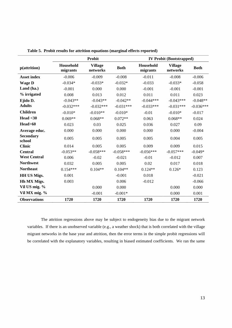
Table 5. Probit results for attrition equations (marginal effects reported)

Probit IV Probit (Bootstrapped)

p(attrition) Household migrants

Village networks

Both Household migrants

Village networks

Both

Asset index -0.006 -0.009 -0.008 -0.011 -0.008 -0.006

Wage D -0.034* -0.033* -0.032* -0.033 -0.033* -0.058 Land (ha.) -0.001 0.000 0.000 -0.001 -0.001 -0.001 % irrigated 0.008 0.013 0.012 0.011 0.011 0.023 Ejido D. -0.043** -0.043** -0.042** -0.044*** -0.043*** -0.048**Adults -0.032*** -0.032*** -0.031*** -0.033*** -0.031*** -0.036***Children -0.010* -0.010** -0.010* -0.01 -0.010* -0.017 Head <30 0.069** 0.068** 0.072** 0.063 0.068** 0.024 Head>60 0.023 0.03 0.025 0.036 0.027 0.09

Average educ. 0.000 0.000 0.000 0.000 0.000 -0.004 Secondary school

0.005 0.005 0.005 0.005 0.004 0.005

Clinic 0.014 0.005 0.005 0.009 0.009 0.015 Central -0.053** -0.058*** -0.058*** -0.056*** -0.057*** -0.049* West Central 0.006 -0.02 -0.021 -0.01 -0.012 0.007 Northwest 0.032 0.005 0.005 0.02 0.017 0.018 Northeast 0.154*** 0.104** 0.104** 0.124** 0.126* 0.123

HH US Migs. 0.001 -0.001 0.018 -0.021

Hh MX Migs. 0.003 0.006 -0.012 -0.066 Vil US mig. % 0.000 0.000 0.000 0.000 Vil MX mig. % -0.001 -0.001* 0.000 0.001

Observations 1720 1720 1720 1720 1720 1720

The attrition regressions above may be subject to endogeneity bias due to the migrant network

variables. If there is an unobserved variable (e.g., a weather shock) that is both correlated with the village

migrant networks in the base year and attrition, then the error terms in the simple probit regressions will

be correlated with the explanatory variables, resulting in biased estimated coefficients. We ran the same

14

probit regressions using instruments for the potentially endogenous village network variables.6 We use

data on GDP per capita in the destination states (both in the US and Mexico) to construct instruments for

village networks similar to those in Orrenius et al. (2009). Our IVs are weighted averages of GDP growth

in migrant destination states over the 5 years following the first round of the survey. We use the share of

migrants from each village (v) in each state (j and k) in 2002 as weights, where j and k are indices for all

states in the US and Mexico, respectively, to create the IVs as follows:7

5102 06

,1

3202 06

,1

v US vj jj

v MX vk kk

IV Share Migs GDPgrowth

IV Share Migs GDPgrowth

(3)

We argue that the changes in the GDP of the states where migrants of a village started out in 2002

affect whole-household migration only through their influence on migration networks. We report the

results of the attrition regressions using these instruments in Table 6. These regressions are carried out

using the divprob command in Stata 10. This program does not provide detailed diagnostics for

instrumental validity; therefore we also run the regressions with a linear probability model (LPM) using

two-step GMM estimation with robust standard errors (ivreg2 with gmm2s option in Stata 10, as

explained in Baum et al., 2007) in order to test for instrumental validity. The results of these tests are

reported in appendix Tables A1 and A2.8 Table A1 reports the coefficients of the IVs in the first step

regressions, indicating that the IVs are rightly correlated with the endogenous variables. We reject under-

and weak identification and fail to reject the hypothesis that the orthogonality conditions are valid (Table

A2). Moreover, the Wald test results reported at the bottom of Table 6 show that the error terms of the

first step regressions do not contain extra variation that is correlated with attrition; hence, the IVs are

6 The income variable can also be potentially endogenous for similar reasons. We ran both sets of regressions (without and with IVs) excluding the per capita income variable that treats the remaining physical capital variables as a reduced form indicator of wealth. The coefficients of the non-IV regressions showed some difference from the results in Table 5, however, all coefficients were virtually the same after instrumenting for the network variables. Therefore, we present the results that include the income variable following the the literature on attrition in panel data (Thomas et al., 2001; Maluccio, 2004).

7 We thank Pia Orrenius for providing us with historical data on GDP, unemployment and other economic indicators for all US states. State level Mexican GDP data is obtained from INEGI: http://dgcnesyp.inegi.org.mx/cgi-win/bdieintsi.exe/NIVR150070#ARBOL

8 We also tried using historical village level migration networks (in 1990) based on the migration histories of households as IVs. This experiment did not change the main results significantly; therefore we only report the results using the weighted GDP growth IVs, because we think that their exogeneity is more intuitive, besides being valid based on the diagnostic tests presented in the appendix Table A2.

15

exogenous to the attrition equation. Based on these test results, we conclude that our instrumental

variables are reasonably valid.

After instrumenting, the coefficient on the US migrant network becomes insignificant in all

instances where it was significant before (i.e., the whole sample, West Central and Northwest regions),

indicating that there was an omitted variable in the error term that was positively correlated with the US

network. The US migration network in the South-Southeast region, however, becomes significant after

instrumenting, making this the only region where whole-household migration is significantly affected by

US migrant networks. All other results in Table 6 are very similar to the un-instrumented results in Table

5. We find that attrition is significantly correlated mainly with the human capital variables and with land

and asset ownership in some regions. Inasmuch as these variables are significantly correlated with

income, analyses of outcome variables based on household income (e.g. inequality and poverty) without

correcting for attrition may be biased.

Fitzgerald et al. (1998) suggest a formal test to identify whether attrition would introduce a

significant bias in the analyses based on the remaining sample. This procedure includes estimating the

outcome regression of interest (income and poverty in our case) using covariates from the first round, a

dummy variable identifying whether the household attrited in the second round and the interactions of this

dummy variable with all covariates. The test for attrition bias then is the joint significance test for all

attrition interactions. If they are significant, this would mean that attriters had different behavioral

patterns from non-attriters before leaving the sample, and hence, analyses of outcome variables based on

non-attriting sample should be corrected for attrition.

We test for attrition bias as suggested by Fitzgerald et al. (1998) using both income and poverty

regressions. We estimate the income regressions using Least Absolute Deviation (LAD) method because

the total income is negative for 33 households and its distribution is right-skewed. After inspecting the

data thoroughly, we decided that these are legitimate negative incomes rather than measurement or

typographical errors. A common procedure to estimate skewed income regressions is to do a logarithmic

transformation, which excludes negative incomes. LAD is another method to decrease the effect of

outliers on the estimated coefficients. We chose the LAD specification in order to not to loose

observations with negative incomes.

16

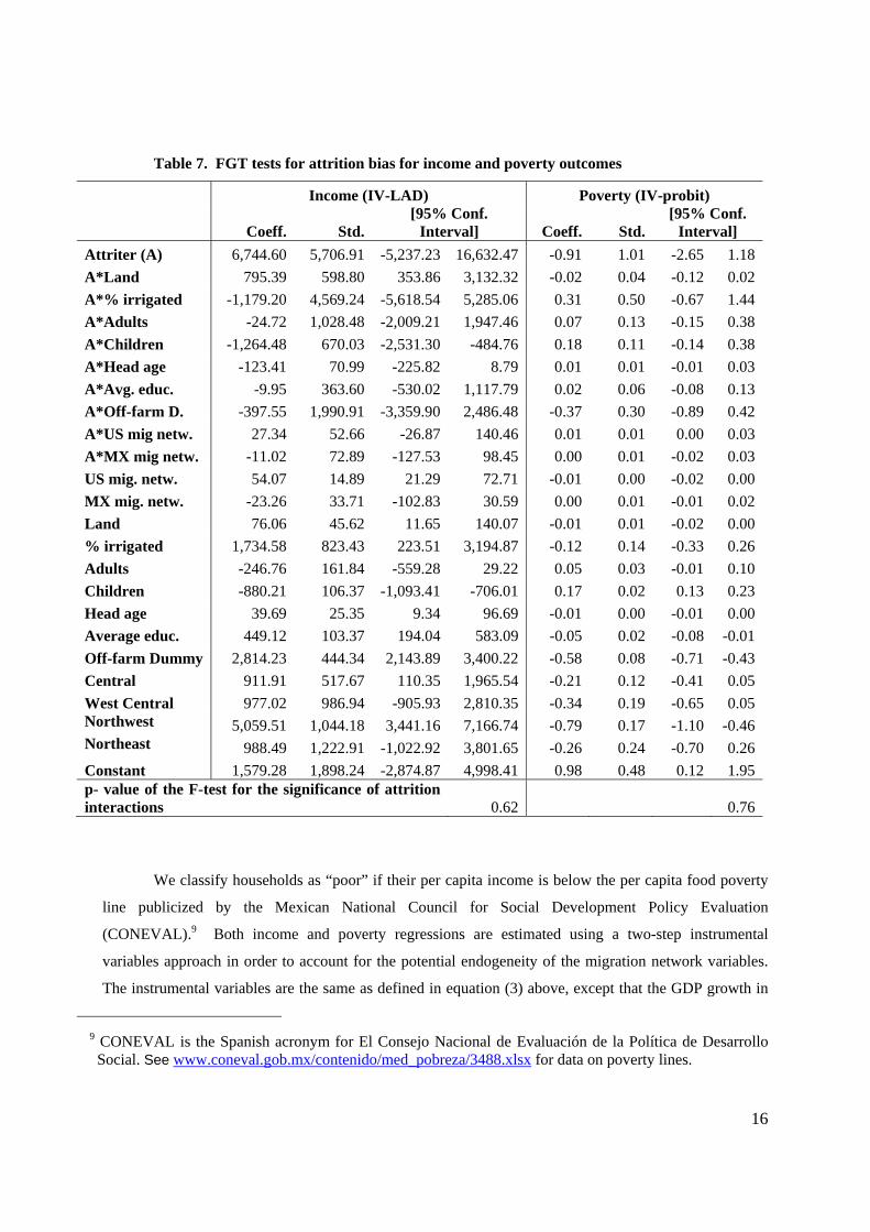
Table 7. FGT tests for attrition bias for income and poverty outcomes

Income (IV-LAD) Poverty (IV-probit)

Coeff. Std.[95% Conf.

Interval] Coeff. Std. [95% Conf.

Interval]

Attriter (A) 6,744.60 5,706.91 -5,237.23 16,632.47 -0.91 1.01 -2.65 1.18

A*Land 795.39 598.80 353.86 3,132.32 -0.02 0.04 -0.12 0.02

A*% irrigated -1,179.20 4,569.24 -5,618.54 5,285.06 0.31 0.50 -0.67 1.44

A*Adults -24.72 1,028.48 -2,009.21 1,947.46 0.07 0.13 -0.15 0.38

A*Children -1,264.48 670.03 -2,531.30 -484.76 0.18 0.11 -0.14 0.38

A*Head age -123.41 70.99 -225.82 8.79 0.01 0.01 -0.01 0.03

A*Avg. educ. -9.95 363.60 -530.02 1,117.79 0.02 0.06 -0.08 0.13

A*Off-farm D. -397.55 1,990.91 -3,359.90 2,486.48 -0.37 0.30 -0.89 0.42

A*US mig netw. 27.34 52.66 -26.87 140.46 0.01 0.01 0.00 0.03

A*MX mig netw. -11.02 72.89 -127.53 98.45 0.00 0.01 -0.02 0.03

US mig. netw. 54.07 14.89 21.29 72.71 -0.01 0.00 -0.02 0.00

MX mig. netw. -23.26 33.71 -102.83 30.59 0.00 0.01 -0.01 0.02

Land 76.06 45.62 11.65 140.07 -0.01 0.01 -0.02 0.00

% irrigated 1,734.58 823.43 223.51 3,194.87 -0.12 0.14 -0.33 0.26

Adults -246.76 161.84 -559.28 29.22 0.05 0.03 -0.01 0.10

Children -880.21 106.37 -1,093.41 -706.01 0.17 0.02 0.13 0.23

Head age 39.69 25.35 9.34 96.69 -0.01 0.00 -0.01 0.00

Average educ. 449.12 103.37 194.04 583.09 -0.05 0.02 -0.08 -0.01

Off-farm Dummy 2,814.23 444.34 2,143.89 3,400.22 -0.58 0.08 -0.71 -0.43

Central 911.91 517.67 110.35 1,965.54 -0.21 0.12 -0.41 0.05

West Central 977.02 986.94 -905.93 2,810.35 -0.34 0.19 -0.65 0.05Northwest 5,059.51 1,044.18 3,441.16 7,166.74 -0.79 0.17 -1.10 -0.46Northeast 988.49 1,222.91 -1,022.92 3,801.65 -0.26 0.24 -0.70 0.26

Constant 1,579.28 1,898.24 -2,874.87 4,998.41 0.98 0.48 0.12 1.95p- value of the F-test for the significance of attrition interactions 0.62 0.76

We classify households as “poor” if their per capita income is below the per capita food poverty

line publicized by the Mexican National Council for Social Development Policy Evaluation

(CONEVAL).9 Both income and poverty regressions are estimated using a two-step instrumental

variables approach in order to account for the potential endogeneity of the migration network variables.

The instrumental variables are the same as defined in equation (3) above, except that the GDP growth in

9 CONEVAL is the Spanish acronym for El Consejo Nacional de Evaluación de la Política de Desarrollo Social. See www.coneval.gob.mx/contenido/med_pobreza/3488.xlsx for data on poverty lines.

17

destination states is for the 5 years preceding the first round of the survey rather than following it. This is

because of the fact that the outcome variables in income and poverty regressions are expected to depend

on historical networks, rather than networks after the first round as in the case of attrition. The results of

these regressions for the whole sample are presented in Table 7. The standard errors are bootstrapped

and the confidence intervals presented are bias corrected.

We fail to reject the hypothesis that the coefficients of attrition interactions jointly equal to zero

in both income and poverty regressions. We conclude that attriters are not significantly different from

non-attriters in terms of their income generating functions and their probabilities of being poor. We also

conducted the same tests for each region separately, and similarly fail to reject the null hypothesis that

attriters and non-attriters are not significantly differ from each other. This result is similar to most

research in the attrition literature that concludes that although attriters and non-attriters may be

significantly different from each other based on some observables, the analyses relying on the remaining

sample in panel studies need not be biased (Alderman et al., 2001; Thomas et al., 2001; Falaris, 2003;

Maluccio, 2004; Baird et al., 2008). Nonetheless, we pay special attention to attrition in our analyses of

the changes in income distribution and poverty in the next section, in order to see the effects of whole-

household migration on these outcomes in rural Mexico between 2002 and 2007.

4. Attrition and changes in inequality and poverty

The central question of this section is how the Gini coefficients, poverty indices and their change

over time are affected by whole-household migration. Following Wooldridge (2002), we use inverse

probability weighting to correct both inequality and poverty indices for attrition.

4.1. Attrition and inequality: We first calculate the Gini coefficients for both years using the

whole sample available in each round. We then calculate the Gini coefficients in 2002 only for those

households that remained in the sample to analyze how attrition affected the change over time in the

income distribution (Table 8).

18

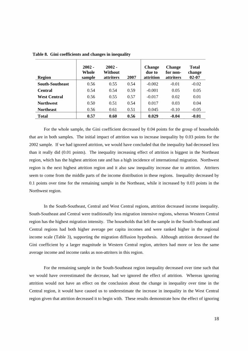
Table 8. Gini coefficients and changes in inequality

Region

2002 - Whole sample

2002 - Without attriters 2007

Change due to

attrition

Change for non-attriters

Total change 02-07

South-Southeast 0.56 0.55 0.54 -0.002 -0.01 -0.02

Central 0.54 0.54 0.59 -0.001 0.05 0.05

West Central 0.56 0.55 0.57 -0.017 0.02 0.01

Northwest 0.50 0.51 0.54 0.017 0.03 0.04

Northeast 0.56 0.61 0.51 0.045 -0.10 -0.05

Total 0.57 0.60 0.56 0.029 -0.04 -0.01

For the whole sample, the Gini coefficient decreased by 0.04 points for the group of households

that are in both samples. The initial impact of attrition was to increase inequality by 0.03 points for the

2002 sample. If we had ignored attrition, we would have concluded that the inequality had decreased less

than it really did (0.01 points). The inequality increasing effect of attrition is biggest in the Northeast

region, which has the highest attrition rate and has a high incidence of international migration. Northwest

region is the next highest attrition region and it also saw inequality increase due to attrition. Attriters

seem to come from the middle parts of the income distribution in these regions. Inequality decreased by

0.1 points over time for the remaining sample in the Northeast, while it increased by 0.03 points in the

Northwest region.

In the South-Southeast, Central and West Central regions, attrition decreased income inequality.

South-Southeast and Central were traditionally less migration intensive regions, whereas Western Central

region has the highest migration intensity. The households that left the sample in the South-Southeast and

Central regions had both higher average per capita incomes and were ranked higher in the regional

income scale (Table 3), supporting the migration diffusion hypothesis. Although attrition decreased the

Gini coefficient by a larger magnitude in Western Central region, attriters had more or less the same

average income and income ranks as non-attriters in this region.

For the remaining sample in the South-Southeast region inequality decreased over time such that

we would have overestimated the decrease, had we ignored the effect of attrition. Whereas ignoring

attrition would not have an effect on the conclusion about the change in inequality over time in the

Central region, it would have caused us to underestimate the increase in inequality in the West Central

region given that attrition decreased it to begin with. These results demonstrate how the effect of ignoring

19

attrition on the analyses of the changes in the income distribution depends on where households that left

the sample stood in the first year of the survey.

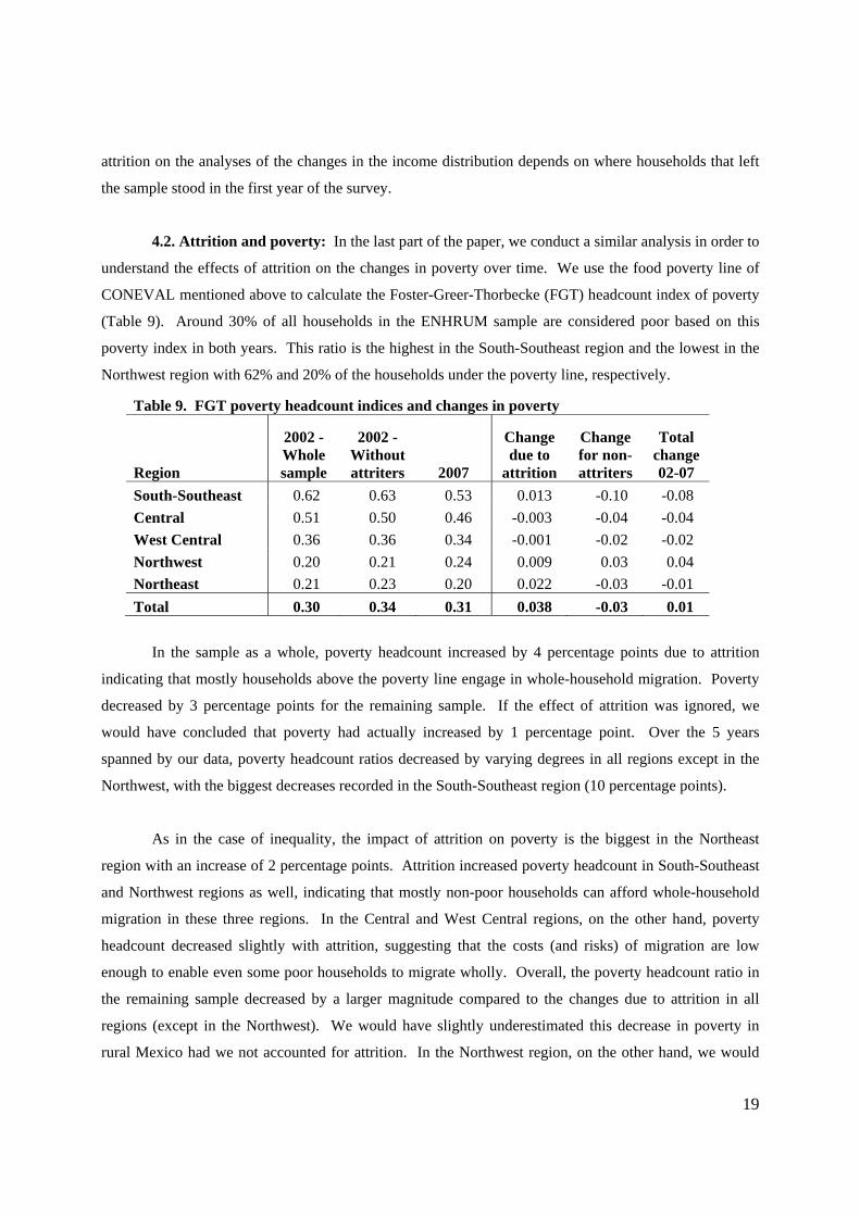
4.2. Attrition and poverty: In the last part of the paper, we conduct a similar analysis in order to

understand the effects of attrition on the changes in poverty over time. We use the food poverty line of

CONEVAL mentioned above to calculate the Foster-Greer-Thorbecke (FGT) headcount index of poverty

(Table 9). Around 30% of all households in the ENHRUM sample are considered poor based on this

poverty index in both years. This ratio is the highest in the South-Southeast region and the lowest in the

Northwest region with 62% and 20% of the households under the poverty line, respectively.

Table 9. FGT poverty headcount indices and changes in poverty

Region

2002 - Whole sample

2002 - Without attriters 2007

Change due to

attrition

Change for non-attriters

Total change 02-07

South-Southeast 0.62 0.63 0.53 0.013 -0.10 -0.08

Central 0.51 0.50 0.46 -0.003 -0.04 -0.04

West Central 0.36 0.36 0.34 -0.001 -0.02 -0.02

Northwest 0.20 0.21 0.24 0.009 0.03 0.04

Northeast 0.21 0.23 0.20 0.022 -0.03 -0.01

Total 0.30 0.34 0.31 0.038 -0.03 0.01

In the sample as a whole, poverty headcount increased by 4 percentage points due to attrition

indicating that mostly households above the poverty line engage in whole-household migration. Poverty

decreased by 3 percentage points for the remaining sample. If the effect of attrition was ignored, we

would have concluded that poverty had actually increased by 1 percentage point. Over the 5 years

spanned by our data, poverty headcount ratios decreased by varying degrees in all regions except in the

Northwest, with the biggest decreases recorded in the South-Southeast region (10 percentage points).

As in the case of inequality, the impact of attrition on poverty is the biggest in the Northeast

region with an increase of 2 percentage points. Attrition increased poverty headcount in South-Southeast

and Northwest regions as well, indicating that mostly non-poor households can afford whole-household

migration in these three regions. In the Central and West Central regions, on the other hand, poverty

headcount decreased slightly with attrition, suggesting that the costs (and risks) of migration are low

enough to enable even some poor households to migrate wholly. Overall, the poverty headcount ratio in

the remaining sample decreased by a larger magnitude compared to the changes due to attrition in all

regions (except in the Northwest). We would have slightly underestimated this decrease in poverty in

rural Mexico had we not accounted for attrition. In the Northwest region, on the other hand, we would

20

have overestimated the increase in poverty given that attrition had increased the poverty headcount ratio

to begin with.

5. Conclusions

Attrition in panel data may introduce bias in the analyses based on the remaining sample if

attrition probabilities depend on the outcome variables of interest. We formally model whole-household

migration and test whether households that participate in whole-household migration and those that do

not differ significantly in terms of their income generating functions and poverty probabilities using panel

data from rural Mexico. Using a novel set of instruments for migrant networks, we show that although

these two groups differ from each other significantly along some human capital variables, their behavioral

income generation coefficients do not differ significantly. These results are robust to different functional

form specifications and instruments, and hold both nationally and regionally. We conclude that analyses

of income and poverty based on panel data reduced by attrition need not be biased in the ENHRUM

sample.

We also analyze the effects of attrition on the changes in income distribution and poverty in rural

Mexico between 2002 and 2007. We find that attrition increased both inequality and poverty in the whole

sample, with heterogeneous effects across regions. Attriters in the South-Southeast region come from the

top of the income distribution, hence inequality decreases and poverty increases in the remaining sample

due to attrition. The opposite happens in the northern regions that are also the most attrition prone areas,

where attriters come from the lower and middle parts of the income distribution with an inequality

increasing effect. Poverty also increases due to attrition in these regions, suggesting that households in

the middle of the income distribution (above the poverty line) are more likely to engage in whole-

household migration.

These results provide supporting evidence for the migration diffusion hypothesis from the point

of whole-household migration. To our knowledge, there are no other studies in the literature that test this

hypothesis for the case of whole-household migration, or that analyze the effects of attrition on income

distribution and poverty. Our results also underline the importance of paying due attention to attrition in

studies based on panel data from developing countries, especially in migration prone areas.

21

REFERENCES

Acosta, P.; Calderon, C.; Fajnzylber, P., and Lopez, H. 2008. “What is the impact of international remittances on poverty and inequality in Latin America?” World Development, 36: 89-114. Adams, Jr. R.H. 1989. “Worker Remittances and Inequality in Rural Egypt.” Economic Development and Cultural Change, 38: 45-71. Adams, Jr. R.H., Cuecuecha, A.J., and Page, J. 2008. “The impact of remittances on poverty and inequality in Ghana.” Policy Research Working Paper No. WPS4732, World Bank, January. Alderman, H., Behrman, J., Kohler, H. P., Maluccio, J.A., and Watkins, S.C. 2001. “Attrition in Longitudinal Household Survey Data: Some Tests for Three Developing Country Samples,” Demographic Research, 5(4): 77–124. Arslan, A. and Taylor, J. E. 2010. “Village level inequality, migration and remittances in rural Mexico: How do they change over time?.” Kiel Working Papers, No: 1622, Kiel Institute for the World Economy.

Baird, S., Hamory, J., and Miguel, T. (2008) “Tracking, Attrition and Data Quality in the Kenyan Life Panel Survey Round 1 (KLPS-1).” Working Paper, UC Berkeley, Department of Economics.

Barham, B., and Boucher, S. 1998. “Migration, remittances, and inequality: estimating the net effects of migration on income distribution.” Journal of Development Economics, 55: 307-331. Baum, C.F; Schaffer, M.F. and Stillman, S. 2007. “Enhanced routines for instrumental variables/GMM estimation and testing.” Boston College, Economics Working Paper, No. 667. Falaris, E. M. 2003. “The Effect of Survey Attrition in Longitudinal Surveys: Evidence From Peru, Cote d’Ivoire and Vietnam.” Journal of Development Economics, 70, 133-157. Fitzgerald, J.; Gottschalk, P., and Moffitt, R. 1998. “An Analysis of Sample Attrition in Panel Data: The Michigan Panel Study of Income Dynamics.” The Journal of Human Resources, Special Issue: Attrition in Longitudinal Surveys, 33(2): 251-299. Lillard, L.A., Panis, C.W.A. 1998. “Panel Attrition from the Panel Study of Income Dynamics: Household Income, Marital Status, and Mortality.” The Journal of Human Resources, Special Issue: Attrition in Longitudinal Surveys, 33(2): 437-457. Maluccio, J.A. 2004. “Using Quality of Interview Information to Assess Nonrandom Attrition Bias in Developing-Country Panel Data.” Review of Development Economics, 8(1): 91-109. McKenzie, D., and Rapoport, H. 2007. “Network effects and the dynamics of migration and inequality: Theory and evidence from Mexico.” Journal of Development Economics, 84: 1-4. McKenzie, D., and Sasin, M. 2007. “Migration, remittances, poverty, and human capital: conceptual and empirical challenges.” Policy Research Working Paper Series, No. 4272, The World Bank.

22

Orrenius, P. M., Zavodny, M., Cañas, J. and Coronado, R. 2010. “Do remittances boost economic development? Evidence from Mexican states.” Working Papers 1007, Federal Reserve Bank of Dallas.

Rosenzweig, M., and Binswanger, H. 1994. “Wealth, Weather Risk, and the Consumption and Profitability of Agricultural Investments.” Economic Journal, 103: 56-78. Singh, I., L. Squire, and J. Strauss. 1986. Agricultural Household Models : Extensions, Applications, and Policy. World Bank Research Publication. Baltimore: Johns Hopkins University Press. Stark, O., and S. Yitzhaki. 1982. “Migration, growth, distribution and welfare,” Economics Letters, 10: 243-249. Stark, O., Taylor, J. E., and S. Yitzhaki. 1986. “Remittances and Inequality.” The Economic Journal, 96:722-740. Stark, O. 1991. “The migration of labor.” B.Blackwell, Cambridge, Mass., USA; Oxford, UK, 406 p. Taylor, J. E. 1992. “Remittances and Inequality Reconsidered: Direct, Indirect and Intertemporal Effects.” Journal of Policy Modeling, 14:187-208. Taylor, J.E., and P.L. Martin. 2001. “Human Capital: Migration and Rural Population Change.” In B. L. Gardner and G. C. Rausser, eds. Handbook of Agricultural Economics. Elsevier Science. Taylor, J.E., and I. Adelman. 2003. “Agricultural Household Models: Genesis, Evolution and Extensions.” Review of Economics of the Household,1:33–58. Taylor, J. E. 2006. “International Migration and Economic Development.” In International Symposium on International Migration and Development. Taylor, J. E.; Mora, J.; Adams, R., and Lopez-Feldman, A. 2008. “Remittances, Inequality and Poverty: Evidence from Rural Mexico.” Migration and Development Within and Across Borders : Research and Policy Perspectives on Internal and International Migration. Josh DeWind and Jennifer Holdaway, eds. Geneva, Switzerland: International Organization for Migration; New York: Social Science Research Council, 191-128. Thomas, D., Frankenberg, E., and Smith, J. P. 2001. “Lost But Not Forgotten: Attrition in the Indonesian Family Life Survey,” Journal of Human Resources, 36(3): 556–92.

Wooldridge, J. M. 2002. “Inverse probability weighted M-estimators for sample selection, attrition, and stratification.” Portuguese Economic Journal, 1(2): 117-139.

23

APPENDIX:

Table A1. Coefficients of the excluded IVs and the R-squared of the first steps of the ivprobit All South-SE Central West Central Northwest Northeast

Coef. p-val Coef. p-val Coef. p-val Coef. p-val Coef. p-val Coef. p-val Dep var: US migrant network Weighted MX state growth rate 39.69 0.33 672.18 0.00 -82.53 0.47 -868.09 0.00 -192.83 0.00 971.80 0.00 Weighted US state growth rate 864.14 0.00 1259.83 0.00 1108.65 0.00 -36.40 0.84 1339.97 0.00 -56.11 0.57 Adj. R-squared 0.72 0.76 0.88 0.78 0.82 0.89 Dep var: MX migrant network Weighted MX state growth rate 477.33 0.00 371.36 0.00 2281.02 0.00 485.21 0.00 18.78 0.71 712.02 0.00 Weighted US state growth rate 20.43 0.62 -36.48 0.58 605.54 0.00 -585.31 0.00 -43.61 0.67 -27.20 0.67 Adj. R-squared 0.86 0.92 0.93 0.97 0.87 0.86

Note: Coefficients of other right hand side variables are not reported. All control variables in table 6 are included in the first stage regressions as well.

24

Table A2. Instrumental Validity tests from 2-step GMM Linear Probability Models for attrition with robust SEs

(Summary results for first-stage regressions of ivreg2 routine in Stata)

All South-SE

Central West Central

North-west*

North-east*

First stage regressions P-val. P-val. P-val. P-val. P-val. P-val.

US mig. network: F-test of joint significance for IVs 0.000 0.000 0.000 0.000 0.000 0.000

MX mig. network: F-test of joint significance for IVs 0.000 0.001 0.000 0.000 0.000 0.000

Underidentification test

Ho: matrix of reduced form coefficients has rank=K1-1 (underidentified)

Ha: matrix has rank=K1 (identified) P-val. P-val. P-val. P-val. P-val. P-val.

Kleibergen-Paap rk LM statistic. Chi-sq(1)=142.63 0.000 0.003 0.000 0.000 0.000 0.000

Kleibergen-Paap rk Wald statistic. Chi-sq(1)=196.84 0.000 0.000 0.000 0.000 0.000 0.000

Weak identification test

Ho: equation is weakly identified

Kleibergen-Paap Wald rk F statistic** 86.87 5.97 31.17 9.23 18.61 36.07

Weak-instrument-robust inference

Tests of joint significance of endogenous regressors B1 in main equation

Ho: B1=0 and overidentifying restrictions are valid P-val P-val P-val P-val P-val P-val

Anderson-Rubin Wald test. F(2,1697)=0.69 0.795 0.095 0.773 0.915 0.744 0.998

Anderson-Rubin Wald test. Chi-sq(2)=1.39 0.793 0.084 0.764 0.911 0.728 0.998

Stock-Wright LM S statistic. Chi-sq(2)=1.38 0.794 0.091 0.767 0.912 0.730 0.998Notes: * The regressions for Northeast and Northwest regions include village local migrant networks in 1990 as an additional IV to avoid underidentification otherwise. ** The critical values of the Kleibergen-Paap rk F Statistic are 4.58 and 7.03 for 15% and 10% maximal IV sizes, respectively.