Which Methods Do We Need for Intensive Longitudinal Data?€¦ · Which Methods Do We Need for Intensive Longitudinal Data? ... mentioned early in the story and will return in a ...

Which Methods Do We Needfor Intensive Longitudinal Data?

Bengt Muthen

Tihomir Asparouhov & Ellen Hamaker

[email protected]

www.statmodel.com

Keynote address at the Modern Modeling Methods ConferenceUConn, May 24, 2016

Expert assistance from Noah Hastings is acknowledged

Bengt Muthen Methods for Intensive Longitudinal Data 1/ 67

The Transitional Aspect of Snow (Foreshadowing)

“Foreshadowing or guessing ahead is a literary device by which an author hints what

is to come. Foreshadowing is a dramatic device in which an important plot-point is

mentioned early in the story and will return in a more significant way. It is used to

avoid disappointment. It is also sometimes used to arouse the reader”.


Non-Intensive versus Intensive Longitudinal Data

Non-intensive longitudinal data:T small (2 - 10) and N largeModeling: Auto-regression and growth

Intensive longitudinal data:T large (30-200) and N smallish (even N = 1) but can be 1,000.Often T > NModeling: We shall see


Intensive Longitudinal Data Collection

Ecological momentary assessment (EMA): a research participantrepeatedly reports on symptoms, affect, behavior, and cognitionsclose in time to experience and in the participants’ naturalenvironment using smartphone, handheld computer, or GPS

Experience sampling method (ESM): a research procedure forstudying what people do, feel, and think during their daily lives

Daily diary measurements

Burst of measurement

Ambulatory assessment (Trull & Ebner-Priemer, 2014. CurrentDirections in Psychological Science)


Examples of Intensive Longitudinal Data Sets

Data Sets N T

Trull data in Jahng et al. (2008)Mood: 84 76-186

Bergeman data in Wang et al. (2012)Positive and negative affect: 230 56

Shiffman data in Hedeker et al. (2013)Smoking urge: 515 34

Laurenceau data in Jongerling et al. (2015)Positive affect: 96 42


Publications on Analysis of Intensive Longitudinal Data

Walls & Schafer (2006). Model for Intensive Longitudinal Data.New York: Oxford University Press.Bolger & Laurenceau (2013). Intensive Longitudinal Methods:An Introduction to Diary and Experience Sampling Research.New York: Guilford.Jahng, Wood & Trull (2008). Analysis of affective instability inecological momentary assessment. Indices using successivedifferences and group comparison via multilevel modeling.Psychological MethodsWang, Hamaker & Bergeman (2012). Investigatinginter-individual differences in short-term intra-individualvariability. Psychological MethodsJongerling, Laurenceau & Hamaker (2015). A multilevel AR(1)model: Allowing for inter-individual differences in trait-scores,inertia, and innovation variance. Multivariate BehavioralResearch


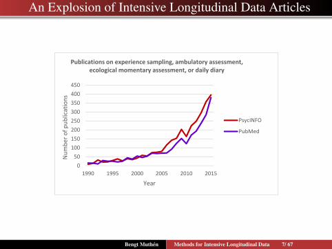
An Explosion of Intensive Longitudinal Data Articles

0

50

100

150

200

250

300

350

400

450

1990 1995 2000 2005 2010 2015

Number of publications

Year

Publications on experience sampling, ambulatory assessment, ecological momentary assessment, or daily diary

PsycINFO

PubMed


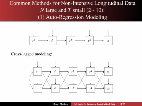
Common Methods for Non-Intensive Longitudinal DataN large and T small (2 - 10):

(1) Auto-Regression Modeling

y1 y2 y3 y4 y5

Cross-lagged modeling:

y1 y2 y3 y4 y5

z1 z2 z3 z4 z5


Common Methods for Non-Intensive Longitudinal Data:(2) Growth Modeling

y1 y2 y3 y4 y5

i

s

0.0 0.5 1.0 1.5 2.0 2.5 3.0

05

1015

Individual Curves

Time

y ou

tcom

e


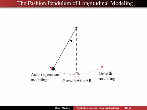
The Fashion Pendulum of Longitudinal Modeling

Auto-regressionmodeling

GrowthmodelingGrowth with AR


Growth Modeling using Single-level Wide Format

y1 y2 y3 y4 y5

i

s

w


Growth Modeling Adding Correlated Residuals

y1 y2 y3 y4 y5

i

s

w


Growth Modeling Adding Auto-Regression (ALT Model)

y1 y2 y3 y4 y5

i

s

w


Growth Modeling Adding Auto-Regressive Residuals

y1 y2 y3 y4 y5

i

s

w


Relating Auto-Regressive and Growth Modeling

Hamaker (2005). Conditions for the equivalence of theautoregressive latent trajectory model and a latent growth curvemodel with autoregressive disturbances. Sociological Methods& Research, 33, 404-416

Jongerling & Hamaker (2011). On the trajectories of thepredetermined ALT model: What are we really modeling?Structural Equation Modeling, 18, 370-382.


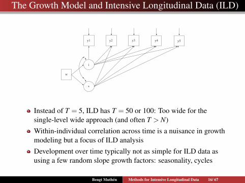
The Growth Model and Intensive Longitudinal Data (ILD)

y1 y2 y3 y4 y5

i

s

w

Instead of T = 5, ILD has T = 50 or 100: Too wide for thesingle-level wide approach (and often T > N)

Within-individual correlation across time is a nuisance in growthmodeling but a focus of ILD analysis

Development over time typically not as simple for ILD data asusing a few random slope growth factors: seasonality, cycles


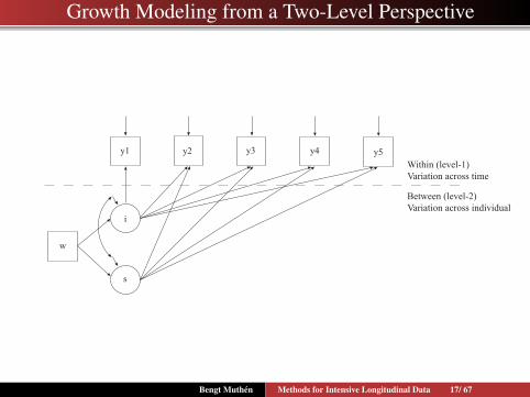
Growth Modeling from a Two-Level Perspective

y1 y2 y3 y4 y5

i

s

w

Within (level-1)Variation across time

Between (level-2)Variation across individual


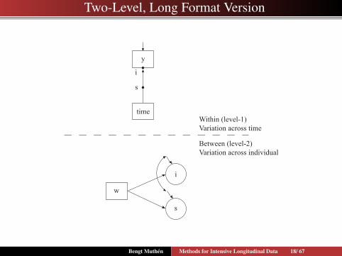
Two-Level, Long Format Version



time

y

w

i

i

s

s


Two-Level, Time-Series Version

t-1

w

y

z

y yty t+1



φ φ

φ

3 key features: Random mean (y), random autoregression (φ ),random variance (not shown)


3 Key Features of Two-Level Time-Series Model:Inter-Individual Differences in Intra-Individual Characteristics

1 Random mean: Individual differences in level2 Random autoregression: Inertia (resistance to change). Related

to:Neuroticism and agreeableness (Suls et al., 1998)Depression (Kuppens et al., 2010)Rumination, self-esteem, life satisfaction, pos. and neg. affect(gender)

3 Random variance: Innovation varianceIndividual differences in reactivity (stress sensitivity) andexposure


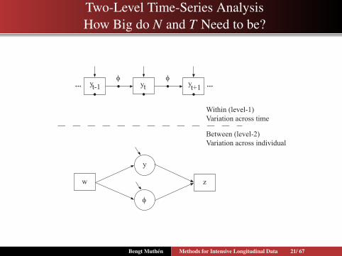
Two-Level Time-Series AnalysisHow Big do N and T Need to be?

t-1

w

y

z

y yty t+1



φ φ

φ


Two-Level Time-Series Analysis:Monte Carlo Simulation Input for Mplus V8

MONTECARLO: NAMES = y w z;NOBSERVATIONS = 5000;NREP = 1000;NCSIZES = 1;CSIZES = 100(50); ! N=100, T= 50LAGVARIABLES = y(1);BETWEEN = w z;

ANALYSIS: TYPE = TWOLEVEL RANDOM;ESTIMATOR = BAYES;BITERATIONS = (1000);PROCESSORS = 2;! MODEL MONTECARLO omitted

MODEL: %WITHIN%phi | y ON y&1*0.5;y*1;%BETWEEN%! w*1;y ON w*.3;y*0.09;phi ON w*.1;phi*.01; [phi*.3];z ON y*.5 phi*.7;z*0.0548;


Two-Level Time-Series Analysis:Monte Carlo Simulations in Mplus V8

t-1

w

y

z

y yty t+1



φ φ

φ

E(φ ) = 0.3, V(φ ) = 0.02, 1000 replications. Ignorable bias, goodcoverage in all cases. Power results:

N = 25, T = 50: φ on w = 0.73, z on φ = 0.15N = 50, T = 50: φ on w = 0.96, z on φ = 0.32N = 100, T = 50: φ on w = 1.00, z on φ = 0.58N = 200, T = 50: φ on w = 1.00, z on φ = 0.87


What About Other Methods for Intensive Longitudinal Data:Part 1. Multilevel Analysis

Papers/talks:Hedeker (2015): Keynote address at the 2015 M3 meetingHedeker, Mermelstein & Demirtas (2012). Modelingbetween-subject and within-subject variances in ecologicalmomentary assessment data using mixed-effects location scalemodels. Statistics in MedicineHedeker & Nordgren (2013). MIXREGLS: A program formixed-effect location scale analysis. Journal of StatisticalSoftware

Data from MIXREGLS:Positive mood related to alone (tvc) and gender (tic), N = 515,T = 34 (3−58)


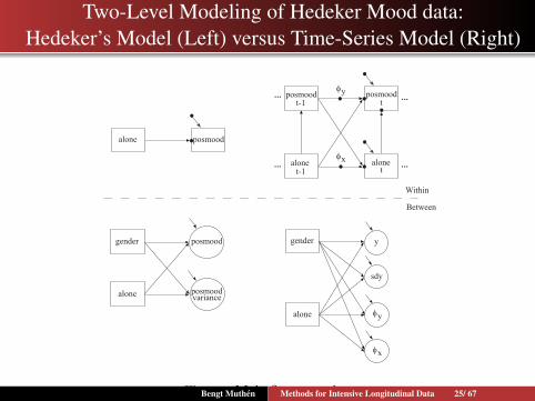
Two-Level Modeling of Hedeker Mood data:Hedeker’s Model (Left) versus Time-Series Model (Right)

Within

Between

alone posmood

posmood posmood

alone alone

t-1 t

tt-1

φx

φy

gender posmood

alone posmoodvariance

gender

alone

y

sdy

φx

φy

Figure : Main figure captionBengt Muthen Methods for Intensive Longitudinal Data 25/ 67


The Transitional Aspect of Snow:Temperature and Snow Depth

Bivariate Time-Series Data with a Lagged Effect- Implications for Sledding


This Page Intentionally Left Blank


Sweden Early 70’s:Department of Statistics, Uppsala University

Bengt’s grad school term project related to time-series analysis:Repeated measurements on respiratory problems of 7 dogsFortran program for ML estimation with autoregressive andheteroscedastic residuals


Mediation Analysis: When in Rome...

m

yx

a b

c


Swedish Harvest Data from 1750 - 1850

Page 1 of 1

4/22/2016file:///C:/Users/Gryphon/Desktop/meadow.gif

Sources:

Thomas (1940). Social and Economic Aspects of SwedishPopulation Movements, 1790 - 1933

McCleary & Hay (1980). Applied Time Series Analysis for theSocial Sciences


Swedish Harvest Data from 1750 - 1850

3 yearly measurements:

Harvest index: Swedish grain harvest rated on a nine-point scale.Total crop failure scored 0; superabundant crop scored 9

Fertility: Births per 1,000 female populationPopulation rate: Birth rate - death rate

Birth rate: the total number of live births per 1,000 of apopulation in a yearDeath rate: the number of deaths per 1,000 of the population in ayear


Time-Series Plots of Harvest, Fertility, and Population Rate

17

40

17

45

17

50

17

55

17

60

17

65

17

70

17

75

17

80

17

85

17

90

17

95

18

00

18

05

18

10

18

15

18

20

18

25

18

30

18

35

18

40

18

45

18

50

18

55

18

60

Year

20

21

22

23

24

25

26

27

28

29

30

31

32

33

34

35

36

Fe

rtil

17

40

17

45

17

50

17

55

17

60

17

65

17

70

17

75

17

80

17

85

17

90

17

95

18

00

18

05

18

10

18

15

18

20

18

25

18

30

18

35

18

40

18

45

18

50

18

55

18

60

Year

0

1

2

3

4

5

6

7

8

9

10

Ha

rve

st

Figure : Harvest (bottom) andFertility (top)

17

40

17

45

17

50

17

55

17

60

17

65

17

70

17

75

17

80

17

85

17

90

17

95

18

00

18

05

18

10

18

15

18

20

18

25

18

30

18

35

18

40

18

45

18

50

18

55

18

60

Year

-35

-30

-25

-20

-15

-10

-5

0

5

10

15

20

Po

pra

te

17

40

17

45

17

50

17

55

17

60

17

65

17

70

17

75

17

80

17

85

17

90

17

95

18

00

18

05

18

10

18

15

18

20

18

25

18

30

18

35

18

40

18

45

18

50

18

55

18

60

Year

20

21

22

23

24

25

26

27

28

29

30

31

32

33

34

35

36

Fe

rtil

Figure : Fertility (bottom) andPopulation Rate (top)


Demographer Sundbarg’s Hypothesis:Harvest, Fertility, and Population Rate, 1750-1850

Irrespective of which party had gained control, or whetherthe King himself was on the throne, if the harvest was good,marriage and birth rates were high and death ratescomparatively low, that is, the bulk of the of the populationflourished.On the contrary, when the harvest failed, marriage andbirth rates declined and death devastated the land, bearingwitness to need and privation and at times even tostarvation. Whether the factories fared well or badly orwhether the bank-rate rose or fell - all the things at thistime, were scarcely more than ripples on the surface(Thomas, 1940: 82).


Theory for how Harvest Influences Fertility

Thomas (1940) cites a number of plausible mechanisms forthis relationship.First, in years following crop failure, marriage rates (andhence, fertility rates) drop.Second, and more importantly, in years following a cropfailure, young women who might otherwise bear children inSweden are likely to emigrate (primarily to Finland and theUnited States during this period).As a result of emigration, the average age of the femalepopulation rises dramatically in years following a cropfailure and fertility drops accordingly.


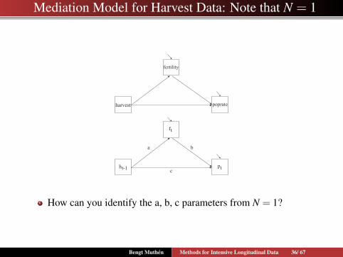
Mediation Model for Harvest Data: Note that N = 1

fertility

poprateharvest

f

ph

t

tt-1

a b

c

How can you identify the a, b, c parameters from N = 1?


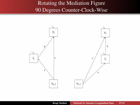
Rotating the Mediation Figure90 Degrees Counter-Clock-Wise

f

p

h

t

t

t-1

c

b

a

p

h

t

t-1

ft

a

b

c


Time-Series Mediation Model (N = 1):Harvest, Fertility, and Population Rate, 1750 - 1850

f

p

h

t

t-1

ft-1

pt-1 pt+1

ht

ft t+1

ht-2

a

b

c


Mplus Version 8 Time-Series Inputfor Swedish Harvest Data: N = 1, T = 102

DATA: FILE = swedish harvest data.txt;VARIABLE: NAME = year harvest fertil poprate;

USEVARIABLES = harvest-poprate;MISSING = all (999);LAGVARIABLES = harvest(1) fertil(1) poprate(1);

DEFINE: fertil = fertil/10;ANALYSIS: ESTIMATOR = BAYES;

PROCESSORS = 2;BITERATIONS = (10000);

MODEL: poprate ON fertil (b)harvest&1;fertil ON harvest&1 (a);! auto-regressive part:poprate ON poprate&1;fertil ON fertil&1;harvest ON harvest&1;

MODEL CONSTRAINT:NEW(indirect);indirect = a*b;


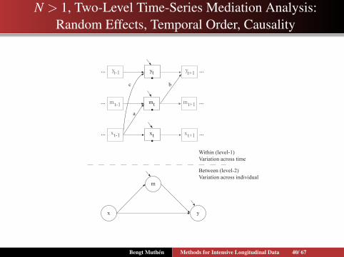
N > 1, Two-Level Time-Series Mediation Analysis:Random Effects, Temporal Order, Causality

t-1

m

x xtx t+1



t-1m mtm t+1

t-1y yty t+1

yx

a

bc


Longitudinal Mediation

Maxwell et al. (2007; 2011): Cross-sectional mediation analysisdoes not capture indirect/direct effects of longitudinal mediationprocesses

822 MAXWELL, COLE, MITCHELL

FIGURE 1 Longitudinal mediation model with one unit lag for direct effect of X on Y

(Model 1).

The path diagram in Figure 1 can be written more formally in terms of the

following equations:

Mi tC1 D mMi t C aXi t C ©MitC1 (1)

Yi tC1 D yYi t C bMi t C cXi t C ©Y itC1 (2)

FIGURE 2 Longitudinal mediation model with two unit lag for direct effect of X on Y

(Model 2).

Dow

nloa

ded

by [

Uni

vers

ity o

f C

alif

orni

a, L

os A

ngel

es (

UC

LA

)], [

Noa

h H

astin

gs]

at 1

1:24

17

May

201

6

Special 2011 issue of Multivariate Behavioral Research (editorS. West; comments by Reichardt, Shrout, Imai et al.)What is missing? - Random effects: Variation across subjects inmean, variance, and auto-regression


Interventions and Time-Series Analysis

N = 1: Implications for ABAB designsBulte & Onghena (2008). An R package for single-caserandomization tests. Behavior Research Methods

Susan Murphy: Just-In-Time Adaptive Interventions (JITAIs) inwhich real-time, passively or actively collected, information on thepatient (e.g., Ecological Momentary Assessments: EMA) is used toinform the real-time delivery of intervention options (e.g.,recommendations, information and prompts)

ARIMA impact assessment: transfer functions


Causal Inference for Time-Series Models:Counterfactually-Defined Causal Effects

(Robins, Pearl, VanderWeele, Imai, Vansteelandt)

N = 1 case versus N > 1 case

Time-varying treatments (exposure), time-varying confoundingMarginal structural models and inverse probability weighting:

Robins et al. (2000). Marginal structural models and causalinference in epidemiology. EpidemiologyVanderWeele et al. (2011). A marginal structural model analysisfor loneliness: Implications for intervention trials and clinicalpractice. Journal of Consulting and Clinical PsychologyVandecandeleare et al. (2016). Time-varying treatments inobservational studies: Marginal structural models of the effects ofearly grade retention on math achievement. MultivariateBehavioral Research

Granger causality (cross-lagged modeling)



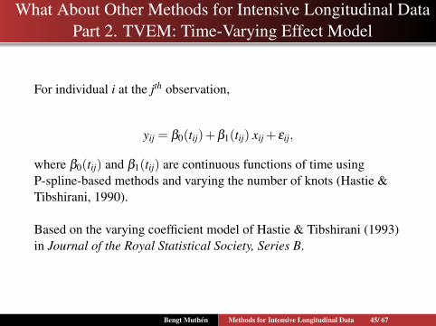
What About Other Methods for Intensive Longitudinal DataPart 2. TVEM: Time-Varying Effect Model

For individual i at the jth observation,

yij = β0(tij)+β1(tij) xij + εij,

where β0(tij) and β1(tij) are continuous functions of time usingP-spline-based methods and varying the number of knots (Hastie &Tibshirani, 1990).

Based on the varying coefficient model of Hastie & Tibshirani (1993)in Journal of the Royal Statistical Society, Series B.


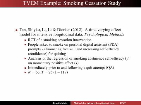
TVEM Example: Smoking Cessation Study

Tan, Shiyko, Li, Li & Dierker (2012). A time varying effectmodel for intensive longitudinal data. Psychological Methods

RCT of a smoking cessation interventionPeople asked to smoke on personal digital assistant (PDA)prompts - eliminating free will and increasing self-efficacy(confidence) for quittingAnalysis of the regression of smoking abstinence self-efficacy (y)on momentary positive affect (x)Immediately prior to and following a quit attempt (QA)N = 66, T = 25 (1−117)


Tan et al. (2012), Continued

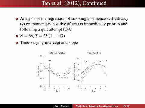
Analysis of the regression of smoking abstinence self-efficacy(y) on momentary positive affect (x) immediately prior to andfollowing a quit attempt (QA)

N = 66, T = 25 (1−117)

Time-varying intercept and slope

of a covariate should be interpreted with reference to a specifictime interval.

The P-spline-based method was employed to progressively fitthe specified model. The number of knots for intercept and slopefunctions was varied, and changes in BIC and AIC fit indices werecompared to determine the best fitting model.

Results. Table 3 presents values of BIC and AIC indices formodels with zero through five knots. Based on the smallest BICand AIC criteria, the model with a single knot for the intercept andslope function parameters was identified as the best fitting model.More complicated models (knots � 5) were not considered due toprogressive worsening of the fit indices (i.e., increasing AIC andBIC). Since both intercept and slope functions were estimated witha single-knot TVEM, Equations 7 and 8, which define the shapesof the functions, would simplify to contain only one additionalterm a3�t � �4�

2, where a single knot K � 1 is placed at 4 days,a point that splits the study time into two equal intervals (a defaultoption in the TVEM macro).

Parameter estimates of the final model are summarizedgraphically in Figure 5. Because of the fluctuating magnitudeand direction of intercept and slope parameters, it appears thattime serves an important role in defining the model. In thegraphical summary of the intercept function, we can see thatindividuals who reported zero positive affect experienced adecrease in self-efficacy following their QA. Initially, theywere more than moderately (self-efficacy � 2) confident intheir ability to refrain from smoking in the postsurgical period,but they gradually transitioned to being less than moderately(self-efficacy � 2) confident. There was a slight increase inintercept function toward the study end with a widening confi-dence interval, which is attributable to more sparse observa-tions. Thus, interpretation of this change should be cautious.Likely, self-efficacy is leveling off toward the end.

The slope function shows that the effect of positive affect onquitting self-efficacy increased with time. Prior to the QA, the effectof positive affect ranged somewhere from .14 to .26; following theQA, it ranged from .26 to .39, signifying an increased associationbetween positive affect and one’s self-efficacy to abstain from smok-ing. Similarly to the intercept function, temporal changes toward theend of study are likely to be an artifact of data sparseness.

Implications From Empirical Data

Self-efficacy toward smoking cessation has been long con-sidered one of the defining factors of success in quitting smok-

ing (e.g., Dornelas, Sampson, Gray, Waters, & Thompson,2000; Gritz et al., 1999; Houston & Miller, 1997; Ockene et al.,2000; Smith, Kraemer, Miller, DeBusk, & Taylor, 1999; Taylor,Houston-Miller, Killen, & DeBusk, 1990; Taylor et al., 1996).Some cross-sectional studies explored correlates of self-efficacy, with positive affect being one of them (e.g., Martinezet al., 2010). Negative affect has been previously linked with anincrease in smoking urges postquit (e.g., Li et al., 2006; Shiff-man, Paty, Gnys, Kassel, & Hickcox, 1996), but no studies haveexplored possible time-varying associations between negativeaffect and self-efficacy.

Based on the results of TVEM, time was shown to play an impor-tant role in defining the strength of the association between positiveaffect and self-efficacy. Overall, individuals with higher levels ofpositive affect reported higher self-efficacy. This relationship wasmagnified, however, following the QA. This finding may suggest thatfuture smoking-cessation intervention strategies could target a pa-tient’s positive affect around the QA. Traditional approaches likemultilevel modeling would estimate the average effect of positiveaffect on self-efficacy. However, the flexibility of TVEM allowed fora full exploration of the relationship without setting a priori con-straints on the shape of intercept and association functions.

In this example, a model with one knot was sufficient to de-scribe the relationship. In other words, these estimated coefficientfunctions were piecewise (two pieces to be exact) quadratic func-tions, which can be represented as

�0�t� � a0 � a1t � a2t2 � a3�t � 4��

2 , �1�t� � b0 � b1t � b2t2

� b3�t � 4��2 ;

since the single knot was placed at � � 4 in this example whenK � 1. It might be reasonable to hypothesize that these coefficientfunctions can be represented by cubic or quartic functions. Thisimplies that TVEM can be used as an exploratory tool to hint atwhether the course of changes follows a certain familiar paramet-ric form. In this study, however, we are reluctant to try higherorder polynomials due to the Runge phenomenon.

Discussion

In this article, we introduced TVEM as a novel approach foranalyzing ILD to study the course of change. With technological

Intercept Function

−3 0 3 6 9 12

1.0

1.5

2.0

2.5

3.0

Sel

f−E

ffica

cy

Days

QA

Slope Function

−3 0 3 6 9 12

0.0

0.1

0.2

0.3

0.4

0.5

Cha

nge

in S

elf−

Effi

cacy

Days

QA

Figure 5. Intercept (left plot) and slope (right plot) function estimates forthe empirical data. In each plot, the solid line represents the estimatedintercept or slope function, and the dotted lines represent the 95% confi-dence interval of the estimated function. QA � quit attempt.

Table 3Fit Statistics for the TVEM Fitted to Self-Efficacy and PositiveAffect Empirical Data

K BIC AIC

0 3,996.3 3,963.81 3,994.6 3,957.22 4,000.9 3,960.83 4,002.6 3,960.34 4,002.1 3,960.45 4,002.2 3,960.5

Note. K is the number of knots for the truncated power splines. Numbers in boldare the minimal Akaike information criterion (AIC) and Bayesian informationcriterion (BIC) values in each column. TVEM � time-varying effect model.

73TIME-VARYING EFFECT MODEL

This

doc

umen

t is c

opyr

ight

ed b

y th

e A

mer

ican

Psy

chol

ogic

al A

ssoc

iatio

n or

one

of i

ts a

llied

pub

lishe

rs.

This

arti

cle

is in

tend

ed so

lely

for t

he p

erso

nal u

se o

f the

indi

vidu

al u

ser a

nd is

not

to b

e di

ssem

inat

ed b

road

ly.


What’s Missing in Regular TVEM?

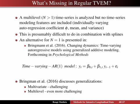
A multilevel (N > 1) time-series is analyzed but no time-seriesmodeling features are included (individually-varyingauto-regression coefficient φ , mean, and variance)

This is presumably difficult to do in combination with splinesAn alternative for N = 1 is presented in:

Bringmann et al. (2016). Changing dynamics: Time-varyingautoregressive models using generalized additive modeling.Forthcoming in Psychological Methods

Time− varying−AR(1) model : yt = β0,t +β1,t yt−1 + εt

Bringman et al. (2016) discusses generalizations:Multivariate - challengingMultilevel - even more challenging


What’s Missing in Regular TVEM?Dynamic Mediation Analysis

Huang & Yuan (2016; online). Bayesian dynamic mediationanalysis. Psychological Methods

Multilevel (N > 1) and multivariateTime-varying coefficients in a mediation modelNonparametric penalized spline approachAutoregressive modeling

What is missing here?

- Continuous-time modeling


Continuous-Time Modeling (CTM):Differential Equations Applied to Mediation Analysis

CTMs applied in a mediation context would allowresearchers to gain insight into how key effects vary as afunction of lag.

Boker & Nesselroade (2002). A method for modeling the intrinsicdynamics of intraindividual variability. Multivariate BehavioralResearch

Voelkle & Oud (2013). Continuous-time modeling withindividually-varying time intervals. British Journal of Mathematicaland Statistical Psychology

Voelkle & Oud (2015). Relating latent change score and continuoustime models. Structural Equation Modeling

Deboeck & Preacher (2015). No need to be discrete: A method forcontinuous time mediation analysis. Structural Equation Modeling



Time-Series Analysis with Latent Variables:Three Final Model Types

Continuous latent variables:Multilevel (N > 1) cross-lagged analysis with factors measuredby multiple indicatorsCross-classified factor model (time crossed with subject)

Categorical latent variables:Transition modeling (Hidden Markov, regime switching,time-series LTA) with latent class variables


Multilevel Time-Series/Dynamic Factor Analysis

f ft-1 t

fb

Within

Between

φ

φ


Time-Series Factor Analysis

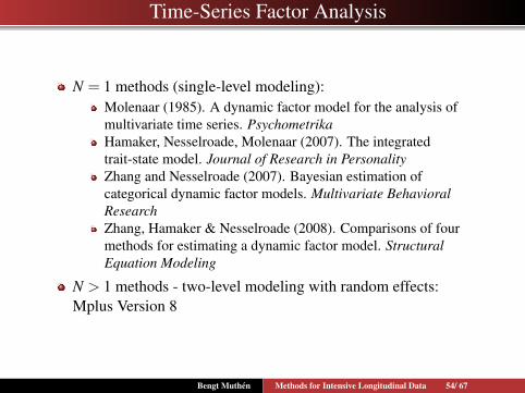
N = 1 methods (single-level modeling):Molenaar (1985). A dynamic factor model for the analysis ofmultivariate time series. PsychometrikaHamaker, Nesselroade, Molenaar (2007). The integratedtrait-state model. Journal of Research in PersonalityZhang and Nesselroade (2007). Bayesian estimation ofcategorical dynamic factor models. Multivariate BehavioralResearchZhang, Hamaker & Nesselroade (2008). Comparisons of fourmethods for estimating a dynamic factor model. StructuralEquation Modeling

N > 1 methods - two-level modeling with random effects:Mplus Version 8


Example: Affective InstabilityIn Ecological Momentary Assessment

Jahng S., Wood, P. K.,& Trull, T. J., (2008). Analysis ofAffective Instability in Ecological Momentary Assessment:Indices Using Successive Difference and Group Comparison viaMultilevel Modeling. Psychological Methods, 13, 354-375

An example of the growing amount of EMA data

84 outpatient subjects: 46 meeting borderline personalitydisorder (BPD) and 38 meeting MDD or DYS

Each individual is measured several times a day for 4 weeks fortotal of about 100 assessments

A mood factor for each individual is measured with 21 self-ratedcontinuous items

The research question is if the BPD group demonstrates moretemporal negative mood instability than the MDD/DYS group


3-Factor EFA/CFA DAFS

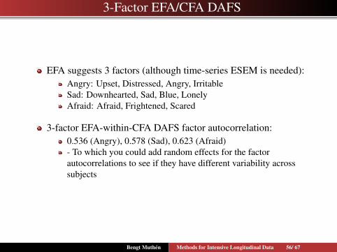
EFA suggests 3 factors (although time-series ESEM is needed):Angry: Upset, Distressed, Angry, IrritableSad: Downhearted, Sad, Blue, LonelyAfraid: Afraid, Frightened, Scared

3-factor EFA-within-CFA DAFS factor autocorrelation:0.536 (Angry), 0.578 (Sad), 0.623 (Afraid)- To which you could add random effects for the factorautocorrelations to see if they have different variability acrosssubjects


Multilevel Cross-Lagged Time-Series Modeling with Factors

WithinBetween

Inter-individual differences

sadt-1

angryt-1

afraidt-1

sadt

angryt

afraidt

t-1

yt-1

yty

+

+

+

yt

ytyt-1

+

How to standardize thecoefficients?

Schuurman et al. (2106).How to comparecross-lagged associations ina multilevel autoregressivemodel. Forthcoming inPsychological Methods


Mplus Version 8 Input for Cross-Lagged Factor Model

ANALYSIS: TYPE = TWOLEVEL RANDOM;ESTIMATOR = BAYES; PROCESSORS = 2; THIN = 5;BITERATIONS = (10000);

MODEL: %WITHIN%f1 BY jittery-scornful*0 (&1);f2 BY jittery-scornful*0 (&1);f3 BY jittery-scornful*0 (&1);f1 BY downhearted*1 sad*1 blue*1 lonely*1;f1 BY angry@0 afraid@0;f2 BY angry*1 irritable*1 hostile*1 scornful*1;f2 BY downhearted@0 afraid@0;f3 BY afraid*1 frightened*1 scared*1;f3 BY downhearted@0 angry@0;f1-f3@1;s1 | f1 ON f1&1;s2 | f2 ON f2&1;s3 | f3 ON f3&1;f1 ON f2&1 f3&1;f2 ON f1&1 f3&1;f3 ON f1&1 f2&1;%BETWEEN%fb BY jittery-scornful*;fb s1-s3 ON group; fb@1;


Cross-Classified Time-Series Factor Analysis

Cross-classification of time and subject gives flexible modeling withrandom intercepts and factor loadings:

Mplus Version 7: Asparouhov & Muthen (2015). General randomeffect latent variable modeling: Random subjects, items, contexts, andparameters. In Harring, Stapleton & Beretvas (Eds.) Advances inmultilevel modeling for educational research: Addressing practicalissues found in real-world applications. Charlotte, NC: InformationAge Publishing, Inc.Mplus Version 8: Expanded to time-series version

Auto-regression for factor and factor indicatorsRandom factor loadings varying across subjects and randomintercepts for measurement and factor intercepts varying acrosstimeCan variation across time in random slopes be used to studytrends?


Cross-Classified Analysis with Factor Variation Across Time:Finding a Trend by Estimating Time-Series Random Slope of

Y on X Using Mplus Version 8 - TVEM-Like Feature

Figure : Intercept Figure : Slope


Time-Series Modeling with Latent Class Variables: N = 1

Latent Transition Analysis (LTA; Hidden Markov model; HMM):

ct-1

t-1na t-1pa tpatna

ct

LTA with autoregression (Markov switching autoreg. model; MSAR):

cct-1

t-1na

t-1pa tpa

tna

t

Hamaker et al. (2016). Modeling BAS dysregulation in bipolardisorder: Illustrating the potential of time series analysis. Assessment


Epilogue: Which Methods Do We Needfor Intensive Longitudinal Data?

What’s the answer?All the above and more

For this we need the input from many researchers


To Learn More About Time-Series Analysis

Classic but only N = 1:Hard: Hamilton (1994), Chatfield (2003)Less hard: Shumway & Stoffer (2011)Quite accessible: Hamaker & Dolan (2009). Idiographic dataanalysis. Book chapter

Accessible, applied writings with N > 1:Chow et al. (2010). Equivalence and differences between SEMand state-space modeling. Structural Equation ModelingJongerling, Laurenceau & Hamaker (2015). A multilevel AR(1)model: Allowing for inter-individual differences in trait-scores,inertia, and innovation variance. Multivariate BehavioralResearchWang, Hamaker & Bergeman (2012). Investigatinginter-individual differences in short-term intra-individualvariability. Psychological MethodsMore in the pipeline


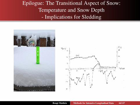
Epilogue: The Transitional Aspect of Snow:Temperature and Snow Depth

- Implications for Sledding






The Transitional Aspect of Snow (Foreshadowing)

“Foreshadowing or guessing ahead is a literary device by which an author hints what

is to come. Foreshadowing is a dramatic device in which an important plot-point is

mentioned early in the story and will return in a more significant way. It is used to

avoid disappointment. It is also sometimes used to arouse the reader”.


Which Methods Do We Need for Intensive Longitudinal Data?€¦ · Which Methods Do We Need for Intensive Longitudinal Data? ... mentioned early in the story and will return in a ...

Documents