A dynamic trajectory class model for intensive longitudinal categorical outcome

Research Article

Received 3 February 2012, Accepted 16 January 2014 Published online 11 February 2014 in Wiley Online Library

(wileyonlinelibrary.com) DOI: 10.1002/sim.6109

A dynamic trajectory class modelfor intensive longitudinalcategorical outcomeHaiqun Lin,a*† Ling Han,b Peter N. Peduzzi,aTerrence E. Murphy,b Thomas M. Gillb and Heather G. Alloreb

This paper presents a novel dynamic latent class model for a longitudinal response that is frequently measuredas in our prospective study of older adults with monthly data on activities of daily living for more than 10 years.The proposed method is especially useful when the longitudinal response is measured much more frequentlythan other relevant covariates. The trajectory classes are latent classes that represent distinct temporal pat-terns of the longitudinal response wherein an individual may remain in a trajectory class or switch to anotheras the class membership predictors are updated periodically over time. The identification of a common set oftrajectory classes allows changes among the temporal patterns to be distinguished from local fluctuations in theresponse. Within a trajectory class, the longitudinal response is modeled by a class-specific generalized linearmixed model. An informative event such as death is jointly modeled by class-specific probability of the eventthrough shared random effects with that for the longitudinal response. We do not impose the conditional inde-pendence assumption given the classes. We illustrate the method by analyzing the change over time in activities ofdaily living trajectory class among 754 older adults with 70,500 person-months of follow-up in the PrecipitatingEvents Project. We also investigate the impact of jointly modeling the class-specific probability of the event onthe parameter estimates in a simulation study. The primary contribution of our paper is the periodic updating oftrajectory classes for a longitudinal categorical response without assuming conditional independence. Copyright© 2014 John Wiley & Sons, Ltd.

Keywords: joint model; intensive longitudinal data; longitudinal categorical data; shared random effects;dynamic latent class; trajectory class

1. Introduction

Many health studies involve conditions whereby individuals make transitions over time among differ-ent health states. In this paper, we use trajectory classes to represent the states describing patterns of acategorical disability measure over time. As an individual survives through successive periods of time,the trajectory classes may change as well and therefore afford the potential updating of the trajectoryclasses, which is a novel feature in this paper.

A longitudinal study of activities of daily living (ADL) among older persons motivated the method-ological development in this article [1–3]. Many authors ascertained ADL status on a monthly basis bytelephone interview and thus an intensively measured longitudinal response. They considered a personto be disabled in ADL if he or she needed help from another person or was unable to complete anyof the basic ADL tasks of walking, bathing, dressing, and transferring. They labeled a person’s ADLresponse as independent if he or she had no disability in any of the four tasks, as mild disability ifone or two ADL tasks were disabled, and as severe disability if three or four ADL tasks were disabled.They obtained more comprehensive health measures such as physical frailty, cognitive status, depressivesymptoms, and chronic diseases through in-home assessments that were conducted at baseline and every18 months there after for more than 10 years.

aDepartment of Biostatistics, Yale School of Public Health, New Haven, CT, U.S.A.bSection of Geriatrics, Department of Internal Medicine, Yale School of Medicine, New Haven, CT, U.S.A.*Correspondence to: Haiqun Lin, 208 LEPH, 60 College Street, New Haven, CT 06520, U.S.A.†E-mail: [email protected]

Copyright © 2014 John Wiley & Sons, Ltd. Statist. Med. 2014, 33 2645–2664

2645

H. LIN ET AL.

Individual ADL trajectories may segregate into distinct patterns within an 18-month interval, andthese patterns may change in the next 18-month time interval. We can capture the evolution of thesedistinct patterns over time by our proposed dynamic latent class model that allows periodic updatingof trajectory class membership within an individual. Studies describe a trajectory pattern within a timeinterval by a class-specific generalized linear mixed model within a general growth mixture modelingframework [4–6]. Within-individual correlation is accounted for by random effects. We model mem-bership in a trajectory class as a polytomous response by using covariates that include baseline andtime-dependent predictors. We update class membership each subsequent time interval as the time-dependent predictors for class are updated. Changes in trajectory class memberships over time signifycorresponding changes in the state of the longitudinal response pattern across time intervals rather thanlocalized fluctuation in the response itself within an time interval. We smooth out the fluctuation by usingthe class-specific regression model within a time interval. Because an event of interest such as deathoccurs during the follow-up and is informatively related to the longitudinal response [7], we account forthe occurrence of the event through modeling trajectory class-specific probability of the event withineach class. So the model for the event occurrence shares random effects with the longitudinal responsethrough factor loadings, in addition to the shared latent classes. Conditioning on the person’s trajectoryclass memberships, we do not assume independence between the longitudinal responses and the eventoccurrence, nor between the longitudinal responses in different time intervals, because of the shared ran-dom effects. Although not explored in this paper, we can alternatively model the event as time to eventfrom baseline (instead of from the end of previous interval). However, it is not straightforward to modelthe class-specific time-to-event outcome because an individual changes his or her class membershipover time.

We do not provide a comprehensive review of the literature on latent class models where class mem-bership for an individual does not change over time. Instead we compare our dynamic latent class modelwith latent transition models (LTMs) [8–14] where class membership is dynamic and changes over time.Our proposed model estimates class membership for trajectory classes repeatedly over time based onupdated predictors, whereas LTMs estimate the transition probabilities among latent classes over time.

The LTMs are sometimes termed as hidden Markov models in which a transition probability isdependent only on the latent class (hidden state) in the preceding time point. Reboussin, Liang, andReboussin [8] studied multiple health indicators with LTMs using estimating equations, and Rijmenet al. [13] and Reboussin and IaLongo [14] estimated the model parameters using maximum likelihood(ML). Miglioretti [9] presented an LTM for multivariate longitudinal responses using a fully Bayesianapproach. Chung, Park and Lanza [10] studied multiple indicators with two latent class variables, andChung, Lanza, and Loken [12] compared estimates in LTMs on the basis of ML [11] and Bayesianinference. Altman [15] used Monte Carlo expectation–maximization algorithm [16] in estimating mixedhidden Markov models with random effects in generalized linear mixed models. LTMs estimate thebaseline probability of class membership and transition probabilities at follow-up time points and typi-cally assign class membership only at baseline. As a result, uncertainty in class membership increaseswith each subsequent time point. In contrast, our dynamic latent trajectory class model estimates trajec-tory class membership over all time intervals simultaneously and directly assigns class membership foreach subsequent interval by incorporating information from time-dependent predictors that are updatedin each time interval. The use of multiple indicators in LTMs does not accommodate missing data ofone or more indicators at a given time point, whereas our proposed model incorporates all availableresponse data.

Our model is similar to the latent class marginal model presented by Reboussin and Anthony [17],which also assigns class membership at all time points without modeling transition probabilities. How-ever, our model differs from theirs in that we estimate the parameters through the method of ML thatallows the number of classes to be chosen through an information criterion while they used estimatingequations to reduce computational burden. In addition, we additionally incorporate random effects andjointly model the probability of informative event—death.

Finally, our approach does not rely on the assumption of local independence, serial independence,or conditional independence given latent classes. The local independence assumption implies that theresponses (e.g., multiple indicators) at a given time point are independent given the latent classes. Theseries independence assumes that longitudinal responses at different time points are independent giventhe latent classes. Conditional independence assumes that responses of different types (e.g., amongmultiple indicators, among multivariate longitudinal responses, or between longitudinal response andthe event of interest in case of joint modeling of longitudinal and event process) are independent given

2646


H. LIN ET AL.

the latent classes. LTMs typically assume local independence. The latent class models for multiple indi-cators ([8,10], growth mixture models [6], and joint models of longitudinal response and risk of an event[18, 19] assume neither local independence nor serial independence by using the random effects withineach latent class; however,these latent class models do assume conditional independence. The joint latentclass models for simultaneous longitudinal response and risk of an event described by Beuckens et al.,Garre et al. and Proust-Lima et al. [20–22] do not assume conditional independence. Uebersax [23]discussed relaxing the conditional independence assumption by including shared random effects acrossdifferent indicators in mixed latent trait model that is adopted in this paper. Jacqmin-Gadda et al. [24]have developed a post hoc score test for assessing the conditional independence assumption in a jointlatent class model.

We organized our paper as follows. In Section 2, we describe our data structure and present ourdynamic latent class model. In Section 3, we specify the ML method of estimation and the assignmentof trajectory class membership. In Section 4, we present the results from the analysis of the ADL dataset. We conduct a simulation study in Section 5, and we conclude with a discussion in Section 6.

2. Methods

2.1. Data structure

The data for our proposed dynamic latent class model typically consist of a frequently measured lon-gitudinal response of interest and less frequent and more comprehensive measures of time-dependentcovariates. Here we use the ADL example of the Precipitating Event Project (PEP) to describe thedata structure.

We indicated the severity of ADL disability by the number of ADL tasks in walking, bathing, dressing,and transferring that the person was unable to carry out independently (from none to four). We consid-ered a person with no disability in any of the four tasks independent, disability in one or two ADL taskswas considered mild, and disability in three or four ADL tasks was considered severe. The PEP data setthat we consider in this article consists of 70,500 person-month follow-up interviews for 126 monthson 754 individuals through June 2010 on the severity of ADL disability. We completed comprehen-sive home-based assessments of functional health measures (e.g., frailty, cognitive status, depression,and chronic diseases) completed at baseline and subsequently at 18-month intervals. We ascertaineddeaths by review of the local obituaries, from the next of kin or another knowledgeable person during asubsequent telephone interview or by both methods [1–3].

We hypothesize a total of C trajectory classes summarizing distinct patterns of the longitudinalresponse of ADL disability over all time intervals. We allow a person’s trajectory class to change overdifferent person intervals, which are defined by the 18-month period between two consecutive compre-hensive in-home interviews when functional health measures were updated. Therefore, the proportionof each trajectory class can change over time, which reflects the evolution of the longitudinal responsepattern rather than local fluctuation that is smoothed out by using model (2).

2.2. Specification for dynamic trajectory class model

We first introduce notation for the responses and covariates. Suppose there are n independent individualsindexed by i D 1; : : : n. We let Yij.m/k denote the indicator of the discrete longitudinal response fallinginto kth category (k D 1; : : : ; K) for person i at time point j nested within interval m (mD 1; : : : ;M )with j D 1; : : : ; Jim, and the time elapsed since the beginning of the interval is denoted by tij.m/. LetDim denote the indicator of the event of interest for person i in interval m. For the example of ADLresponse, we have k D 1, 2, and 3 for no, mild, and severe disabilities, respectively. An older personmight die in an interval, so the minimum and the maximum values of Jim in our data set are 0 and 18,respectively. The minimum and the maximum values of M in our data set are 1 and 7, respectively.

We first specify the membership probability for trajectory class c (c D 1; : : : ; C ) through a polyto-mous logistic regression model. The membership for a trajectory class can be influenced by covariatesand time elapsed since baseline.

log.�imc=�im1/D XTim˛c ; (1)

where �imc denotes the probability of class c for individual i in interval m, Xim is the vector of pre-dictors for trajectory class c for person i in interval m that can include baseline and interval-specific


2647

H. LIN ET AL.

covariates along with their interactions terms, as well as the terms of time as represented by the linearand quadratic terms of the interval index .m � 1/ (see Table III for a listing of covariates). ˛c is thecorresponding vector of regression coefficients specific for class c where c D 1 is the reference class sothat ˛1 D 0. Xim is expressed as .xim1; xim2; : : :/T and ˛c as .˛1c ; ˛2c ; : : :/T.

We then model the class-specific trajectory for a longitudinal categorical response within an intervalm through a generalized linear mixed model for a polytomous response:

log.�ij.m/kc=�ij.m/1c/D ˇTkctij.m/C �

Tkcdiag.bi /tij.m/: (2)

In model (2), �ij.m/kc is the corresponding mean of Yij.m/k at time j if individual i is in class c inintervalm. ˇkc D .ˇ0kc ; ˇ1kc ; ˇ2kc ; : : :/T is a vector of class c-specific fixed regression coefficients for

the vector tij.m/ D�1; tij.m/; t

2ij.m/

; : : :�T

, which contains the intercept and polynomial terms of time

for the kth category of the polytomous response of Y . We can replace the polynomial terms of time canbe replaced with splines. bi D .b0i ; b1i ; b2i ; : : :/

T is a vector of random effects for individual i thatis assumed to be independent normal with mean zero and variance vector � 2 D

��20 ; �

21 ; �

22 ; : : :

�, and

diag.bi / denotes the diagonal matrix with the diagonal elements being bi . �kc D .�0kc ; �1kc ; �2kc ; : : :/T

is a vector of response category k-specific and class c-specific factor loadings for the corresponding ran-dom effects. Because the elements in the vectors ˇ1c and �1c are set to zero for the reference categoryk D 1 (no ADL disability) of the polytomous response, there are a total of C � .K � 1/ vectors forsubmodels in (2) with non-zero ˇ’s and �’s. We set the factor loadings in �21 for the second responsecategory k D 2 in the reference class c D 1 to one to ensure model identifiability.

For an ordinal response, Liu et al. (2010) [25] used Mplus software [26] to fit the growth mixturemodel with two random effects (intercept and slope). Our use of a model for nominal response allowsthe parameters of time trends and those of the predictors to vary across different ADL categories (i.e.,mild or severe) and thereby avoid a strong and often unrealistic proportional odds assumption that wouldrestrict the parameters (excepting the intercept) to be the same across different categories.

Given the trajectory classes for a given interval, the aforementioned specification is similar to that ofthe mixed effect logit model for a longitudinal nominal response described by Hedeker and Gibbon [5] inwhich the variance components of the random effects vary across the different response categories. Wecan handle measurements that are missing at random [27] by the mixed model through ML estimation.However, because the occurrence of an event of interest is regarded as informative, we explicitly modelthe class-specific probability of the event in (3). We do not consider the issue of intermittent missinglongitudinal responses that are missing not at random as it is not a focus of this paper.

Finally, each class has its own probability for the occurrence of an event such as death. We jointlymodel the event with a class-specific logistic model with shared random effects and factor loadings:

logit.pimc/D ı0c C �Tc bSi ; (3)

where pimc is the probability of individual i in class c having the event in interval m and ı0c and�c D .�0c ; �1c ; �2c ; : : :/

T are the class c-specific intercept and the vector of class c-specific factor load-ings for the random effects bSi shared with the longitudinal model (2), respectively. Please note that theelements in bSi are either the same as or a subset of bi . For example, the event submodel may sharethe random intercepts but not the random slopes of time from the longitudinal submodel. Because anindividual changes his or her class memberships over time, it is highly complex if indeed possible, tospecify a class-specific time-to-death model from baseline. So we do not pursue this route in this paper.We do not assume conditional independence given the classes because the random effects are sharedamong different intervals and with the model for death.

A random effect represents a source of variability. It can have different variances by pairing it withdifferent factor loadings. Together, the terms �T

kcbi in (2) and �Tc bSi in (3) can yield a total of K � C

different sets of variabilities associated with the vector of random effects because there are .K � 1/longitudinal response categories within each class and one event that are associated with specific fac-tor loadings. Further imposing a more complex serial correlation structure beyond compound symmetryas implied by the person-specific random effect would add further computational complexity in ourdynamic latent class model.

2648


H. LIN ET AL.

3. Estimation

We use ML methods to simultaneously estimate the parameters in our model. We can write the likelihoodof the observed data (all the longtiudinal ADL responses and the death) under our model as follows:

nYiD1

Zbi

MYmD1

24 CXcD1

8<:�imc

JimYj.m/D1

KYkD1

�Yij.m/kij.m/kc

!9=;pDimimc .1� pimc/

.1�Dim/

35f .bi /dbi ; (4)

where f .bi / is the density function of the random effects vector. The termsQJimj.m/D1

�QKkD1 �

Yij.m/kij.m/kc

�and pDimimc .1 � pimc/

.1�Dim/ are the person i’s likelihood of the longitudinal response and of death,respectively, within interval m conditional on class c and the random effects bi . Because the longitudi-nal response and death also depend on the random effects, they are not conditionally independent giventhe trajectory classes.

3.1. Estimating procedure and determining the number of trajectory classes

The likelihood function given in (4) does not have a closed form solution even though computationof the integral and the summation can be reduced using the expectation–maximization algorithm [16].We numerically maximized the logarithm of the likelihood given in (4). We tried a combination ofdifferent optimization techniques and integration methods using SAS proc nlmixed [28] in orderto obtain stable parameter estimates. ML estimates using the non–adaptive Gauss-Hermite quadraturewith 40 fixed points for integration and the Newton–Raphson ridging optimization almost always con-verged for our models using the criteria for the quadratic form in the gradient and the inverse Hessianat gconv D 10�6. We obtained standard errors of the parameter estimates by numerically inverting thenegative Hessian matrix. SAS IML Studio can be used to invoke proc nlmixed as well. The SASproc nlmixed code for estimating our models is given in the Appendix.

We started our estimation with one trajectory class model of C D 1, which can be regarded as atypical joint model of a longitudinal nominal response and a binary event. We used the estimates fromone trajectory class model plus additional parameter values of ˛’s, ˇ’s, �’s, ı’s, and �’s for a secondclass as the initial values for fitting two-class models; the additional set of parameters were set to severaldifferent combinations of zeros and ones to give different sets of initial values. Similarly, the estimatesfrom the best of two trajectory-class models plus additional parameter values of ˛’s, ˇ’s, �’s, ı’s and� for a third class were then used as the initial values for three-class models, and so on. The purposeof multiple sets of initial values was to avoid local maxima. For a given C , we set the model with thelargest log-likelihood value as the best and final model for that C .

To determine the optimal number of trajectory classes, C , we fit models with increasing C , and wedeclare C as our final number of trajectory classes when the BIC of the C -class model was smaller thanthe BIC for both the models with class number of C �1 and C C1, respectively. WE calculated the BICon the basis of the number of person intervals, not the number of persons.

3.2. Determining membership for trajectory class

We assigned trajectory class membership for person i in interval m to the trajectory class that has themaximum of Q�imc for c D 1; : : : ; C , where Q�imc is the posterior probability of being in trajectory classc given the observed data of the longitudinal responses and the event outcome of death:

Q�imc D P.Classim D cjYim;Dim/;

D�imcf .Yim;DimjClassim D c/PCcD1 �imcf .Yim;DimjClassim D c/

; (5)

where Classim is the class membership of person i in interval m and Yim represents the longitudinalresponse for person i within interval m, that is, Yim D .Yij.m/k; j D 1; : : : ; JimI k D 1; : : : ; K/. Theterm f .Yim;DimjClassim D c/ is the likelihood of person i’s data within interval m conditional onclass c only:


2649

H. LIN ET AL.

f .Yim;DimjClassim D c/;DZ

bi

JimYj.m/D1

KYkD1

�Yij.m/kij.m/kc

!pDimimc .1� pimc/

.1�Dim/f .bi /dbi : (6)

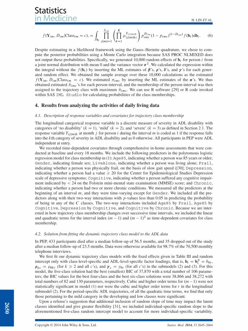
Despite estimating in a likelihood framework using the Gauss–Hermite quadrature, we chose to com-pute the posterior probabilities using a Monte Carlo integration because SAS PROC NLMIXED doesnot output these probabilities. Specifically, we generated 10,000 random effects of bi for person i froma joint normal distribution with mean 0 and the variance vector � 2. We calculated the expression withinthe integral without the f .bi / by inserting the ML estimates of ˇ’s, �’s, ı’s, and �’s for each gener-ated random effect. We obtained the sample average over these 10,000 calculations as the estimatedf .Yim;DimjClassim D c/. We estimated �imc by inserting the ML estimates of the ˛’s. We thusobtained estimated Q�imc’s for each person-interval, and the membership of the person-interval was thenassigned to the trajectory class with maximum Q�imc . We can use R software [29] or R code invokedwithin SAS IML Studio for calculating probabilities of the class memberships.

4. Results from analyzing the activities of daily living data

4.1. Description of response variables and covariates for trajectory class membership

The longitudinal categorical response variable is a discrete measure of severity in ADL disability withcategories of ‘no disability’ (k D 1), ‘mild’ (k D 2), and ‘severe’ (k D 3) as defined in Section 2.1. Theresponse variable Yij.m/k at month j for person i during the intervalm is coded as 1 if the response fallsinto the kth category of severity in ADL disability and as 0 otherwise. All participants in PEP were ADLindependent at entry.

We recorded time-dependent covariates through comprehensive in-home assessments that were con-ducted at baseline and every 18 months. We include the following predictors in the polytomous logisticregression model for class membership in (1): Age85, indicating whether a person was 85 years or older;Gender, indicating female sex; LiveAlone, indicating whether a person was living alone; Frail,indicating whether a person was physically frail, on the basis of slow gait speed ([30]; Depression,indicating whether a person had a value > 20 for the Center for Epidemiological Studies Depressionscale of depressive symptoms; Cognitive, indicating whether a person suffered any cognitive impair-ment indicated by < 24 on the Folstein mini-mental state examination (MMSE) score; and Chronic,indicating whether a person had two or more chronic conditions. We measured all the predictors at thebeginning of an interval m, and they were time-varying except for Gender. We included all the pre-dictors along with their two-way interactions with p-values less than 0.05 in predicting the probabilityof being in any of the C classes. The two-way interactions included Age85 by Frail, Age85 byCognitive, Depression by Cognitive, and Cognitive by Chronic. Because we are inter-ested in how trajectory class membership changes over successive time intervals, we included the linearand quadratic terms for the interval index (m � 1/ and .m � 1/2 as time-dependent covariates for classmembership.

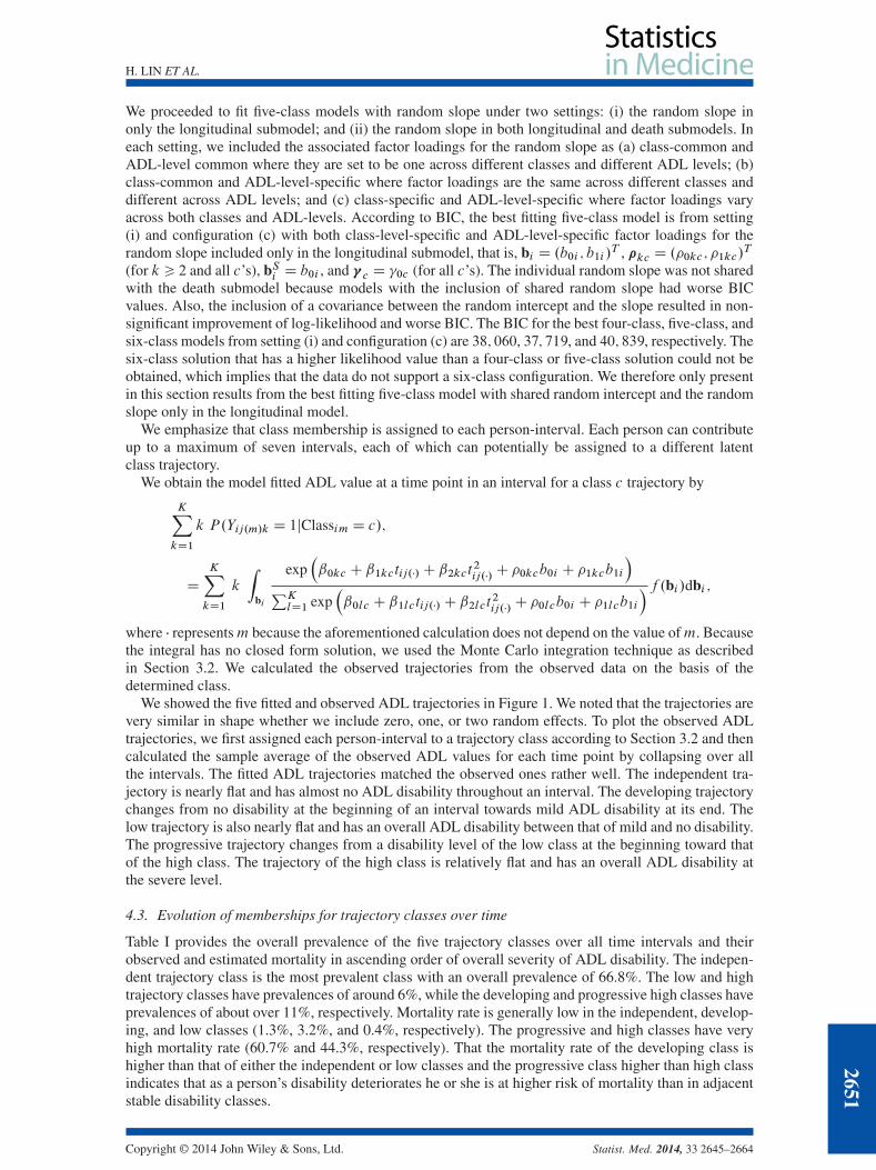
4.2. Solution from fitting the dynamic trajectory class model to the ADL data

In PEP, 433 participants died after a median follow-up of 56.5 months, and 35 dropped out of the studyafter a median follow-up of 23.5 months. Data were otherwise available for 98.7% of the 70,500 monthlytelephone interviews.

We first fit our dynamic trajectory class models with the fixed effects given in Table III and randomintercept only with class-level-specific and ADL-level-specific factor loadings, that is, bi D bSi D b0i ,�kc D �0kc (for k > 2 and all c’s), and �c D �0c (for all c’s) in the submodels (2) and (3). For thismodel, the five-class solution had the best (smallest) BIC of 37,870 with a total number of 106 parame-ters; the BIC values for the best four-class and the best six-class solutions were 38,866 and 38,272 withtotal numbers of 82 and 130 parameters, respectively. Cubic and higher order terms for .m�1/ were notstatistically significant in model (1) nor were the cubic and higher order terms for t in the longitudinalsubmodel (2). For the period-specific ADL trajectories, of all the quadratic time terms, we find that onlythose pertaining to the mild category in the developing and low classes were significant.

Upon a referee’s suggestion that additional inclusion of random slope of time may impact the latentclasses identified and give greater flexibility [31], we included individual-specific random slope to theaforementioned five-class random intercept model to account for more individual-specific variability.

2650


H. LIN ET AL.

We proceeded to fit five-class models with random slope under two settings: (i) the random slope inonly the longitudinal submodel; and (ii) the random slope in both longitudinal and death submodels. Ineach setting, we included the associated factor loadings for the random slope as (a) class-common andADL-level common where they are set to be one across different classes and different ADL levels; (b)class-common and ADL-level-specific where factor loadings are the same across different classes anddifferent across ADL levels; and (c) class-specific and ADL-level-specific where factor loadings varyacross both classes and ADL-levels. According to BIC, the best fitting five-class model is from setting(i) and configuration (c) with both class-level-specific and ADL-level-specific factor loadings for therandom slope included only in the longitudinal submodel, that is, bi D .b0i ; b1i /T , �kc D .�0kc ; �1kc/

T

(for k > 2 and all c’s), bSi D b0i , and �c D �0c (for all c’s). The individual random slope was not sharedwith the death submodel because models with the inclusion of shared random slope had worse BICvalues. Also, the inclusion of a covariance between the random intercept and the slope resulted in non-significant improvement of log-likelihood and worse BIC. The BIC for the best four-class, five-class, andsix-class models from setting (i) and configuration (c) are 38; 060, 37; 719, and 40; 839, respectively. Thesix-class solution that has a higher likelihood value than a four-class or five-class solution could not beobtained, which implies that the data do not support a six-class configuration. We therefore only presentin this section results from the best fitting five-class model with shared random intercept and the randomslope only in the longitudinal model.

We emphasize that class membership is assigned to each person-interval. Each person can contributeup to a maximum of seven intervals, each of which can potentially be assigned to a different latentclass trajectory.

We obtain the model fitted ADL value at a time point in an interval for a class c trajectory by

KXkD1

k P.Yij.m/k D 1jClassim D c/;

D

KXkD1

k

Zbi

exp�ˇ0kc C ˇ1kctij.�/C ˇ2kct

2ij.�/C �0kcb0i C �1kcb1i

�PKlD1 exp

�ˇ0lc C ˇ1lctij.�/C ˇ2lct

2ij.�/C �0lcb0i C �1lcb1i

�f .bi /dbi ;

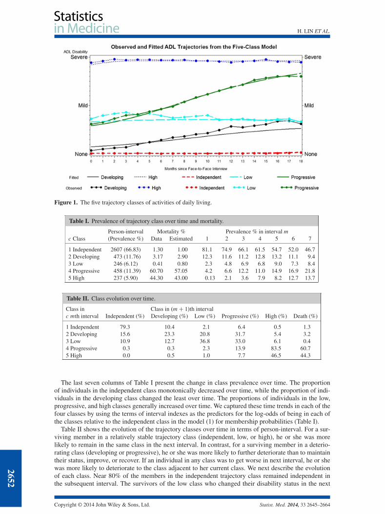
where � representsm because the aforementioned calculation does not depend on the value ofm. Becausethe integral has no closed form solution, we used the Monte Carlo integration technique as describedin Section 3.2. We calculated the observed trajectories from the observed data on the basis of thedetermined class.

We showed the five fitted and observed ADL trajectories in Figure 1. We noted that the trajectories arevery similar in shape whether we include zero, one, or two random effects. To plot the observed ADLtrajectories, we first assigned each person-interval to a trajectory class according to Section 3.2 and thencalculated the sample average of the observed ADL values for each time point by collapsing over allthe intervals. The fitted ADL trajectories matched the observed ones rather well. The independent tra-jectory is nearly flat and has almost no ADL disability throughout an interval. The developing trajectorychanges from no disability at the beginning of an interval towards mild ADL disability at its end. Thelow trajectory is also nearly flat and has an overall ADL disability between that of mild and no disability.The progressive trajectory changes from a disability level of the low class at the beginning toward thatof the high class. The trajectory of the high class is relatively flat and has an overall ADL disability atthe severe level.

4.3. Evolution of memberships for trajectory classes over time

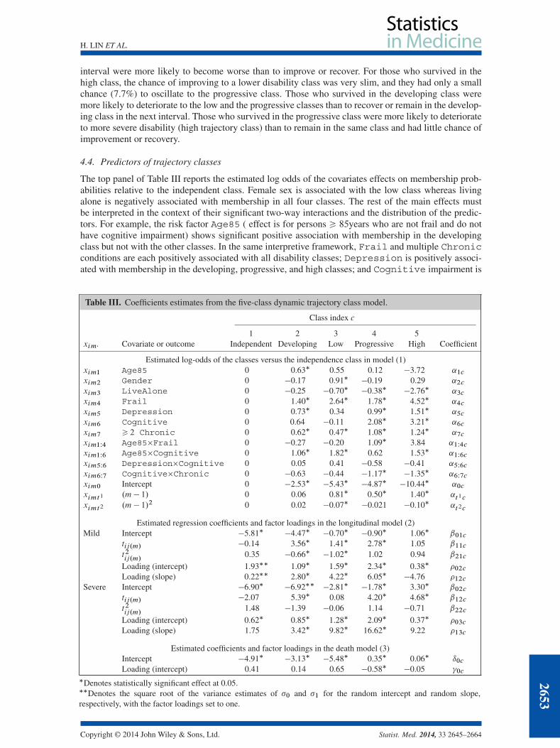
Table I provides the overall prevalence of the five trajectory classes over all time intervals and theirobserved and estimated mortality in ascending order of overall severity of ADL disability. The indepen-dent trajectory class is the most prevalent class with an overall prevalence of 66.8%. The low and hightrajectory classes have prevalences of around 6%, while the developing and progressive high classes haveprevalences of about over 11%, respectively. Mortality rate is generally low in the independent, develop-ing, and low classes (1.3%, 3.2%, and 0.4%, respectively). The progressive and high classes have veryhigh mortality rate (60.7% and 44.3%, respectively). That the mortality rate of the developing class ishigher than that of either the independent or low classes and the progressive class higher than high classindicates that as a person’s disability deteriorates he or she is at higher risk of mortality than in adjacentstable disability classes.


2651

H. LIN ET AL.

Figure 1. The five trajectory classes of activities of daily living.

Table I. Prevalence of trajectory class over time and mortality.

Person-interval Mortality % Prevalence % in interval mc Class (Prevalence %) Data Estimated 1 2 3 4 5 6 7

1 Independent 2607 (66.83) 1.30 1.00 81.1 74.9 66.1 61.5 54.7 52.0 46.72 Developing 473 (11.76) 3.17 2.90 12.3 11.6 11.2 12.8 13.2 11.1 9.43 Low 246 (6.12) 0.41 0.80 2.3 4.8 6.9 6.8 9.0 7.3 8.44 Progressive 458 (11.39) 60.70 57.05 4.2 6.6 12.2 11.0 14.9 16.9 21.85 High 237 (5.90) 44.30 43.00 0.13 2.1 3.6 7.9 8.2 12.7 13.7

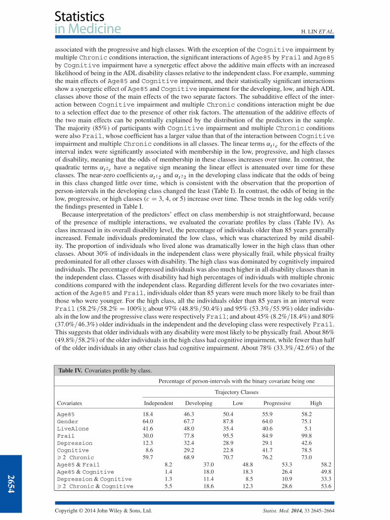
Table II. Class evolution over time.

Class in Class in .mC 1/th intervalc mth interval Independent (%) Developing (%) Low (%) Progressive (%) High (%) Death (%)

1 Independent 79.3 10.4 2.1 6.4 0.5 1.32 Developing 15.6 23.3 20.8 31.7 5.4 3.23 Low 10.9 12.7 36.8 33.0 6.1 0.44 Progressive 0.3 0.3 2.3 13.9 83.5 60.75 High 0.0 0.5 1.0 7.7 46.5 44.3

The last seven columns of Table I present the change in class prevalence over time. The proportionof individuals in the independent class monotonically decreased over time, while the proportion of indi-viduals in the developing class changed the least over time. The proportions of individuals in the low,progressive, and high classes generally increased over time. We captured these time trends in each of thefour classes by using the terms of interval indexes as the predictors for the log-odds of being in each ofthe classes relative to the independent class in the model (1) for membership probabilities (Table I).

Table II shows the evolution of the trajectory classes over time in terms of person-interval. For a sur-viving member in a relatively stable trajectory class (independent, low, or high), he or she was morelikely to remain in the same class in the next interval. In contrast, for a surviving member in a deterio-rating class (developing or progressive), he or she was more likely to further deteriorate than to maintaintheir status, improve, or recover. If an individual in any class was to get worse in next interval, he or shewas more likely to deteriorate to the class adjacent to her current class. We next describe the evolutionof each class. Near 80% of the members in the independent trajectory class remained independent inthe subsequent interval. The survivors of the low class who changed their disability status in the next

2652


H. LIN ET AL.

interval were more likely to become worse than to improve or recover. For those who survived in thehigh class, the chance of improving to a lower disability class was very slim, and they had only a smallchance (7.7%) to oscillate to the progressive class. Those who survived in the developing class weremore likely to deteriorate to the low and the progressive classes than to recover or remain in the develop-ing class in the next interval. Those who survived in the progressive class were more likely to deteriorateto more severe disability (high trajectory class) than to remain in the same class and had little chance ofimprovement or recovery.

4.4. Predictors of trajectory classes

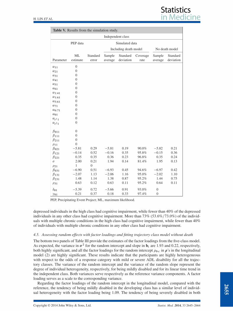
The top panel of Table III reports the estimated log odds of the covariates effects on membership prob-abilities relative to the independent class. Female sex is associated with the low class whereas livingalone is negatively associated with membership in all four classes. The rest of the main effects mustbe interpreted in the context of their significant two-way interactions and the distribution of the predic-tors. For example, the risk factor Age85 ( effect is for persons > 85years who are not frail and do nothave cognitive impairment) shows significant positive association with membership in the developingclass but not with the other classes. In the same interpretive framework, Frail and multiple Chronicconditions are each positively associated with all disability classes; Depression is positively associ-ated with membership in the developing, progressive, and high classes; and Cognitive impairment is

Table III. Coefficients estimates from the five-class dynamic trajectory class model.

Class index c

1 2 3 4 5xim� Covariate or outcome Independent Developing Low Progressive High Coefficient

Estimated log-odds of the classes versus the independence class in model (1)xim1 Age85 0 0.63� 0.55 0.12 �3.72 ˛1cxim2 Gender 0 �0.17 0.91� �0.19 0.29 ˛2cxim3 LiveAlone 0 �0.25 �0.70� �0.38� �2.76� ˛3cxim4 Frail 0 1.40� 2.64� 1.78� 4.52� ˛4cxim5 Depression 0 0.73� 0.34 0.99� 1.51� ˛5cxim6 Cognitive 0 0.64 �0.11 2.08� 3.21� ˛6cxim7 > 2 Chronic 0 0.62� 0.47� 1.08� 1.24� ˛7cxim1W4 Age85�Frail 0 �0.27 �0.20 1.09� 3.84 ˛1W4cxim1W6 Age85�Cognitive 0 1.06� 1.82� 0.62 1.53� ˛1W6cxim5W6 Depression�Cognitive 0 0.05 0.41 �0.58 �0.41 ˛5W6cxim6W7 Cognitive�Chronic 0 �0.63 �0.44 �1.17� �1.35� ˛6W7cxim0 Intercept 0 �2.53� �5.43� �4.87� �10.44� ˛0cximt1 .m� 1/ 0 0.06 0.81� 0.50� 1.40� ˛t1cximt2 .m� 1/2 0 0.02 �0.07� �0.021 �0.10� ˛t2c

Estimated regression coefficients and factor loadings in the longitudinal model (2)Mild Intercept �5.81� �4.47� �0.70� �0.90� 1.06� ˇ01c

tij.m/ �0.14 3.56� 1.41� 2.78� 1.05 ˇ11ct2ij.m/

0.35 �0.66� �1.02� 1.02 0.94 ˇ21c

Loading (intercept) 1.93�� 1.09� 1.59� 2.34� 0.38� �02cLoading (slope) 0.22�� 2.80� 4.22� 6.05� �4.76 �12c

Severe Intercept �6.90� �6.92�� 2.81� �1.78� 3.30� ˇ02ctij.m/ �2.07 5.39� 0.08 4.20� 4.68� ˇ12ct2ij.m/

1.48 �1.39 �0.06 1.14 �0.71 ˇ22c

Loading (intercept) 0.62� 0.85� 1.28� 2.09� 0.37� �03cLoading (slope) 1.75 3.42� 9.82� 16.62� 9.22 �13c

Estimated coefficients and factor loadings in the death model (3)Intercept �4.91� �3.13� �5.48� 0.35� 0.06� ı0cLoading (intercept) 0.41 0.14 0.65 �0.58� �0.05 �0c

�Denotes statistically significant effect at 0.05.��Denotes the square root of the variance estimates of �0 and �1 for the random intercept and random slope,respectively, with the factor loadings set to one.


2653

H. LIN ET AL.

associated with the progressive and high classes. With the exception of the Cognitive impairment bymultiple Chronic conditions interaction, the significant interactions of Age85 by Frail and Age85by Cognitive impairment have a synergetic effect above the additive main effects with an increasedlikelihood of being in the ADL disability classes relative to the independent class. For example, summingthe main effects of Age85 and Cognitive impairment, and their statistically significant interactionsshow a synergetic effect of Age85 and Cognitive impairment for the developing, low, and high ADLclasses above those of the main effects of the two separate factors. The subadditive effect of the inter-action between Cognitive impairment and multiple Chronic conditions interaction might be dueto a selection effect due to the presence of other risk factors. The attenuation of the additive effects ofthe two main effects can be potentially explained by the distribution of the predictors in the sample.The majority (85%) of participants with Cognitive impairment and multiple Chronic conditionswere also Frail, whose coefficient has a larger value than that of the interaction between Cognitiveimpairment and multiple Chronic conditions in all classes. The linear terms ˛t1c for the effects of theinterval index were significantly associated with membership in the low, progressive, and high classesof disability, meaning that the odds of membership in these classes increases over time. In contrast, thequadratic terms ˛t2c have a negative sign meaning the linear effect is attenuated over time for theseclasses. The near-zero coefficients ˛t12 and ˛t22 in the developing class indicate that the odds of beingin this class changed little over time, which is consistent with the observation that the proportion ofperson-intervals in the developing class changed the least (Table I). In contrast, the odds of being in thelow, progressive, or high classes (c D 3, 4, or 5) increase over time. These trends in the log odds verifythe findings presented in Table I.

Because interpretation of the predictors’ effect on class membership is not straightforward, becauseof the presence of multiple interactions, we evaluated the covariate profiles by class (Table IV). Asclass increased in its overall disability level, the percentage of individuals older than 85 years generallyincreased. Female individuals predominated the low class, which was characterized by mild disabil-ity. The proportion of individuals who lived alone was dramatically lower in the high class than otherclasses. About 30% of individuals in the independent class were physically frail, while physical frailtypredominated for all other classes with disability. The high class was dominated by cognitively impairedindividuals. The percentage of depressed individuals was also much higher in all disability classes than inthe independent class. Classes with disability had high percentages of individuals with multiple chronicconditions compared with the independent class. Regarding different levels for the two covariates inter-action of the Age85 and Frail, individuals older than 85 years were much more likely to be frail thanthose who were younger. For the high class, all the individuals older than 85 years in an interval wereFrail (58:2%=58:2%D 100%); about 97% (48:8%=50:4%) and 95% (53:3%=55:9%) older individu-als in the low and the progressive class were respectively Frail; and about 45% (8:2%=18:4%) and 80%(37:0%=46:3%) older individuals in the independent and the developing class were respectively Frail.This suggests that older individuals with any disability were most likely to be physically frail. About 86%(49:8%=58:2%) of the older individuals in the high class had cognitive impairment, while fewer than halfof the older individuals in any other class had cognitive impairment. About 78% (33:3%=42:6%) of the

Table IV. Covariates profile by class.

Percentage of person-intervals with the binary covariate being one

Trajectory Classes

Covariates Independent Developing Low Progressive High

Age85 18.4 46.3 50.4 55.9 58.2Gender 64.0 67.7 87.8 64.0 75.1LiveAlone 41.6 48.0 35.4 40.6 5.1Frail 30.0 77.8 95.5 84.9 99.8Depression 12.3 32.4 28.9 29.1 42.6Cognitive 8.6 29.2 22.8 41.7 78.5> 2 Chronic 59.7 68.9 70.7 76.2 73.0Age85 & Frail 8.2 37.0 48.8 53.3 58.2Age85 & Cognitive 1.4 18.0 18.3 26.4 49.8Depression & Cognitive 1.3 11.4 8.5 10.9 33.3> 2 Chronic & Cognitive 5.5 18.6 12.3 28.6 53.6

2654


H. LIN ET AL.

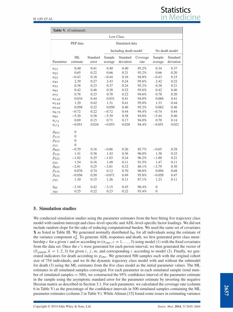
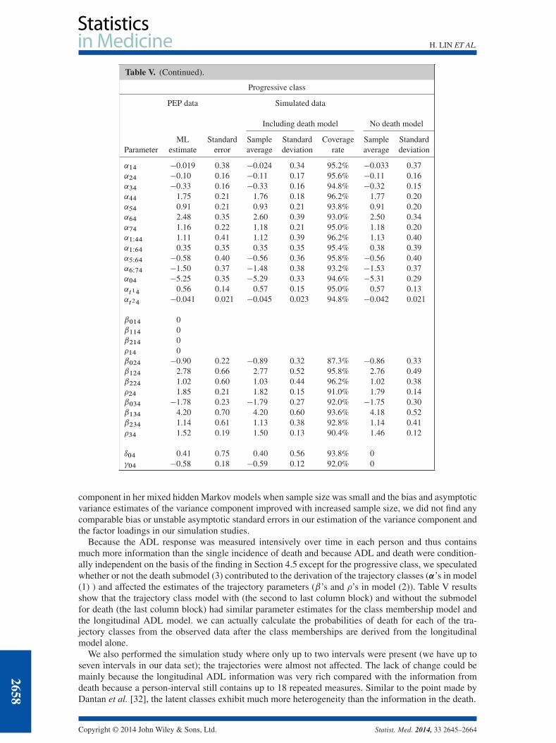
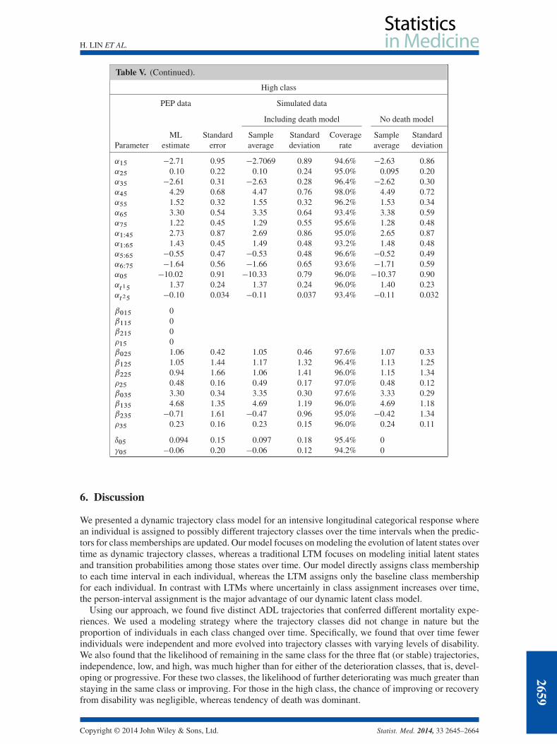
Table V. Results from the simulation study.

Independent class

PEP data Simulated data

Including death model No death model

ML Standard Sample Standard Coverage Sample StandardParameter estimate error average deviation rate average deviation

˛11 0˛21 0˛31 0˛41 0˛51 0˛61 0˛1W41 0˛1W61 0˛5W61 0˛71 0˛6W71 0˛01 0˛t11 0˛t21 0

ˇ011 0ˇ111 0ˇ211 0�11 0ˇ021 �5.81 0.29 �5.81 0.19 90.0% �5.82 0.21ˇ121 �0.14 0.52 �0.16 0.35 95.8% �0.15 0.36ˇ221 0.35 0.35 0.36 0.23 96.8% 0.35 0.24� 2.00 0.21 1.94 0.14 81.4% 1.95 0.13�21 1 0ˇ031 �6.90 0.51 �6.93 0.45 94.6% �6.97 0.42ˇ131 �2.07 1.13 �2.06 1.16 95.0% �2.02 1.10ˇ231 1.48 1.14 1.38 0.87 95.2% 1.44 0.75�31 0.63 0.12 0.63 0.11 95.2% 0.64 0.11

ı01 �5.39 0.72 �5.66 0.91 93.0% 0�01 0.21 0.37 0.18 0.33 97.4% 0

PEP, Precipitating Event Project; ML, maximum likelihood.

depressed individuals in the high class had cognitive impairment, while fewer than 40% of the depressedindividuals in any other class had cognitive impairment. More than 73% (53:6%=73:0%) of the individ-uals with multiple chronic conditions in the high class had cognitive impairment, while fewer than 40%of individuals with multiple chronic conditions in any other class had cognitive impairment.

4.5. Assessing random effects with factor loadings and fitting trajectory class model without death

The bottom two panels of Table III provide the estimates of the factor loadings from the five-class model.As expected, the variance in � 2 for the random intercept and slope in bi are 1.93 and 0.22, respectively,both highly significant, and all the factor loadings for the random intercept �0�c in �’s in the longitudinalmodel (2) are highly significant. These results indicate that the participants are highly heterogeneouswith respect to the odds of a response category with mild or severe ADL disability for all the trajec-tory classes. The variance of the random intercept and the variance of the random slope represent thedegree of individual heterogeneity, respectively, for being mildly disabled and for its linear time trend inthe independent class. Both variances serve respectively as the reference variance components. A factorloading serves as a scale to the corresponding variance.

Regarding the factor loadings of the random intercept in the longitudinal model, compared with thereference, the tendency of being mildly disabled in the developing class has a similar level of individ-ual heterogeneity with the factor loading being 1.09. The tendency of being severely disabled in both


2655

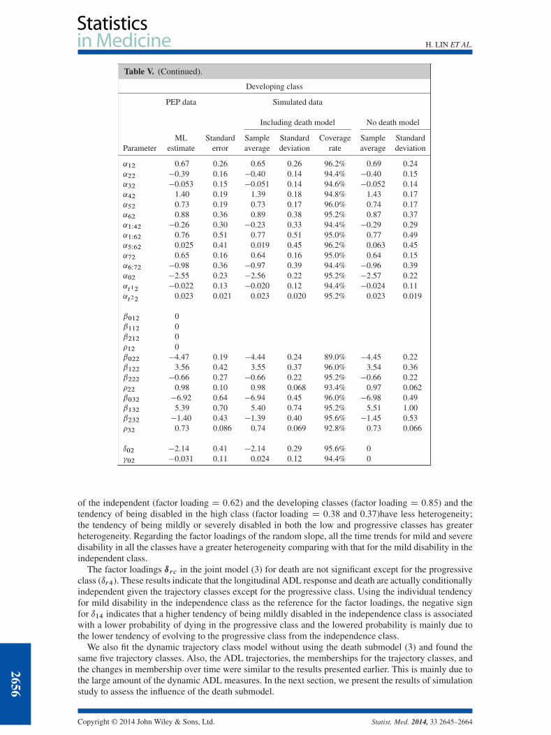
H. LIN ET AL.

Table V. (Continued).

Developing class




˛12 0.67 0.26 0.65 0.26 96.2% 0.69 0.24˛22 �0.39 0.16 �0.40 0.14 94.4% �0.40 0.15˛32 �0.053 0.15 �0.051 0.14 94.6% �0.052 0.14˛42 1.40 0.19 1.39 0.18 94.8% 1.43 0.17˛52 0.73 0.19 0.73 0.17 96.0% 0.74 0.17˛62 0.88 0.36 0.89 0.38 95.2% 0.87 0.37˛1W42 �0.26 0.30 �0.23 0.33 94.4% �0.29 0.29˛1W62 0.76 0.51 0.77 0.51 95.0% 0.77 0.49˛5W62 0.025 0.41 0.019 0.45 96.2% 0.063 0.45˛72 0.65 0.16 0.64 0.16 95.0% 0.64 0.15˛6W72 �0.98 0.36 �0.97 0.39 94.4% �0.96 0.39˛02 �2.55 0.23 �2.56 0.22 95.2% �2.57 0.22˛t12 �0.022 0.13 �0.020 0.12 94.4% �0.024 0.11˛t22 0.023 0.021 0.023 0.020 95.2% 0.023 0.019

ˇ012 0ˇ112 0ˇ212 0�12 0ˇ022 �4.47 0.19 �4.44 0.24 89.0% �4.45 0.22ˇ122 3.56 0.42 3.55 0.37 96.0% 3.54 0.36ˇ222 �0.66 0.27 �0.66 0.22 95.2% �0.66 0.22�22 0.98 0.10 0.98 0.068 93.4% 0.97 0.062ˇ032 �6.92 0.64 �6.94 0.45 96.0% �6.98 0.49ˇ132 5.39 0.70 5.40 0.74 95.2% 5.51 1.00ˇ232 �1.40 0.43 �1.39 0.40 95.6% �1.45 0.53�32 0.73 0.086 0.74 0.069 92.8% 0.73 0.066

ı02 �2.14 0.41 �2.14 0.29 95.6% 0�02 �0.031 0.11 0.024 0.12 94.4% 0

of the independent (factor loading D 0:62) and the developing classes (factor loading D 0:85) and thetendency of being disabled in the high class (factor loading D 0:38 and 0.37)have less heterogeneity;the tendency of being mildly or severely disabled in both the low and progressive classes has greaterheterogeneity. Regarding the factor loadings of the random slope, all the time trends for mild and severedisability in all the classes have a greater heterogeneity comparing with that for the mild disability in theindependent class.

The factor loadings ırc in the joint model (3) for death are not significant except for the progressiveclass (ır4). These results indicate that the longitudinal ADL response and death are actually conditionallyindependent given the trajectory classes except for the progressive class. Using the individual tendencyfor mild disability in the independence class as the reference for the factor loadings, the negative signfor ı14 indicates that a higher tendency of being mildly disabled in the independence class is associatedwith a lower probability of dying in the progressive class and the lowered probability is mainly due tothe lower tendency of evolving to the progressive class from the independence class.

We also fit the dynamic trajectory class model without using the death submodel (3) and found thesame five trajectory classes. Also, the ADL trajectories, the memberships for the trajectory classes, andthe changes in membership over time were similar to the results presented earlier. This is mainly due tothe large amount of the dynamic ADL measures. In the next section, we present the results of simulationstudy to assess the influence of the death submodel.

2656


H. LIN ET AL.


Low Class




˛13 0.40 0.41 0.40 0.40 95.2% 0.34 0.37˛23 0.65 0.22 0.66 0.21 93.2% 0.66 0.20˛33 �0.43 0.18 �0.44 0.16 94.8% �0.43 0.15˛43 2.39 0.27 2.43 0.24 95.6% 2.42 0.22˛53 0.38 0.23 0.37 0.24 95.2% 0.38 0.21˛63 0.42 0.46 0.38 0.52 95.6% 0.42 0.46˛73 0.76 0.23 0.78 0.22 94.6% 0.78 0.20˛1W43 0.034 0.44 0.031 0.41 94.0% 0.068 0.41˛1W63 1.29 0.42 1.31 0.41 95.0% 1.33 0.44˛5W63 0.058 0.22 0.050 0.46 95.2% 0.062 0.46˛6W73 �0.72 0.22 �0.72 0.44 94.4% �0.74 0.44˛03 �5.30 0.38 �5.39 0.38 94.8% �5.44 0.40˛t13 0.69 0.15 0.71 0.17 94.0% 0.70 0.14˛t23 �0.051 0.024 �0.053 0.028 94.4% �0.051 0.021

ˇ013 0ˇ113 0ˇ213 0�13 0ˇ023 �0.70 0.16 �0.66 0.26 85.7% �0.65 0.28ˇ123 1.41 0.38 1.42 0.36 96.0% 1.38 0.32ˇ223 �1.02 0.25 �1.03 0.24 96.2% �1.00 0.21�23 1.54 0.16 1.49 0.11 91.5% 1.47 0.11ˇ033 �2.81 0.25 �2.81 0.32 86.1% �2.79 0.30ˇ133 0.076 0.74 0.12 0.70 96.8% 0.094 0.68ˇ233 �0.056 0.50 �0.071 0.49 95.8% �0.058 0.47�33 1.30 0.15 1.26 0.11 87.1% 1.23 0.11

ı03 �3.10 0.42 �3.15 0.45 96.4% 0�03 0.25 0.22 0.23 0.22 93.4% 0

5. Simulation studies

We conducted simulation studies using the parameter estimates from the best fitting five trajectory classmodel with random intercept and class–level-specific and ADL-level-specific factor loadings. We did notinclude random slope for the sake of reducing computational burden. We used the same set of covariatesX as listed in Table III. We generated normally distributed b0i for all individuals using the estimate ofthe variance component �20 . To generate ADL responses and death, we first generated prior class mem-bership c for a given i andm according to .�imc ; c D 1; : : : ; 5/ using model (1) with the fixed covariatesfrom the data set. Once the c’s were generated for each person interval, we then generated the vector of.Yij.m/k; k D 1; 2; 3/ for given i , j , m, and corresponding c according to model (2). Finally, we gen-erated indicators for death according to pimc . We generated 500 samples each with the original cohortsize of 754 individuals, and we fit the dynamic trajectory class model with and without the submodelfor death (3) using the ML estimates from the five class model as the initial parameter values. The MLestimates in all simulated samples converged. For each parameter in each simulated sample (total num-ber of simulated samplesD 500), we constructed the 95% confidence interval of the parameter estimatein the sample using the asymptotic standard error for the parameter estimate by inverting the negativeHessian matrix as described in Section 3.1. For each parameter, we calculated the coverage rate (column6 in Table V) as the percentage of the confidence intervals in 500 simulated samples containing the MLparameter estimates (column 2 in Table V). While Altman [15] found some issues in estimating variance


2657

H. LIN ET AL.


Progressive class




˛14 �0.019 0.38 �0.024 0.34 95.2% �0.033 0.37˛24 �0.10 0.16 �0.11 0.17 95.6% �0.11 0.16˛34 �0.33 0.16 �0.33 0.16 94.8% �0.32 0.15˛44 1.75 0.21 1.76 0.18 96.2% 1.77 0.20˛54 0.91 0.21 0.93 0.21 93.8% 0.91 0.20˛64 2.48 0.35 2.60 0.39 93.0% 2.50 0.34˛74 1.16 0.22 1.18 0.21 95.0% 1.18 0.20˛1W44 1.11 0.41 1.12 0.39 96.2% 1.13 0.40˛1W64 0.35 0.35 0.35 0.35 95.4% 0.38 0.39˛5W64 �0.58 0.40 �0.56 0.36 95.8% �0.56 0.40˛6W74 �1.50 0.37 �1.48 0.38 93.2% �1.53 0.37˛04 �5.25 0.35 �5.29 0.33 94.6% �5.31 0.29˛t14 0.56 0.14 0.57 0.15 95.0% 0.57 0.13˛t24 �0.041 0.021 �0.045 0.023 94.8% �0.042 0.021

ˇ014 0ˇ114 0ˇ214 0�14 0ˇ024 �0.90 0.22 �0.89 0.32 87.3% �0.86 0.33ˇ124 2.78 0.66 2.77 0.52 95.8% 2.76 0.49ˇ224 1.02 0.60 1.03 0.44 96.2% 1.02 0.38�24 1.85 0.21 1.82 0.15 91.0% 1.79 0.14ˇ034 �1.78 0.23 �1.79 0.27 92.0% �1.75 0.30ˇ134 4.20 0.70 4.20 0.60 93.6% 4.18 0.52ˇ234 1.14 0.61 1.13 0.38 92.8% 1.14 0.41�34 1.52 0.19 1.50 0.13 90.4% 1.46 0.12

ı04 0.41 0.75 0.40 0.56 93.8% 0�04 �0.58 0.18 �0.59 0.12 92.0% 0

component in her mixed hidden Markov models when sample size was small and the bias and asymptoticvariance estimates of the variance component improved with increased sample size, we did not find anycomparable bias or unstable asymptotic standard errors in our estimation of the variance component andthe factor loadings in our simulation studies.

Because the ADL response was measured intensively over time in each person and thus containsmuch more information than the single incidence of death and because ADL and death were condition-ally independent on the basis of the finding in Section 4.5 except for the progressive class, we speculatedwhether or not the death submodel (3) contributed to the derivation of the trajectory classes (˛’s in model(1) ) and affected the estimates of the trajectory parameters (ˇ’s and �’s in model (2)). Table V resultsshow that the trajectory class model with (the second to last column block) and without the submodelfor death (the last column block) had similar parameter estimates for the class membership model andthe longitudinal ADL model. we can actually calculate the probabilities of death for each of the tra-jectory classes from the observed data after the class memberships are derived from the longitudinalmodel alone.

We also performed the simulation study where only up to two intervals were present (we have up toseven intervals in our data set); the trajectories were almost not affected. The lack of change could bemainly because the longitudinal ADL information was very rich compared with the information fromdeath because a person-interval still contains up to 18 repeated measures. Similar to the point made byDantan et al. [32], the latent classes exhibit much more heterogeneity than the information in the death.

2658


H. LIN ET AL.


High class




˛15 �2.71 0.95 �2.7069 0.89 94.6% �2.63 0.86˛25 0.10 0.22 0.10 0.24 95.0% 0.095 0.20˛35 �2.61 0.31 �2.63 0.28 96.4% �2.62 0.30˛45 4.29 0.68 4.47 0.76 98.0% 4.49 0.72˛55 1.52 0.32 1.55 0.32 96.2% 1.53 0.34˛65 3.30 0.54 3.35 0.64 93.4% 3.38 0.59˛75 1.22 0.45 1.29 0.55 95.6% 1.28 0.48˛1W45 2.73 0.87 2.69 0.86 95.0% 2.65 0.87˛1W65 1.43 0.45 1.49 0.48 93.2% 1.48 0.48˛5W65 �0.55 0.47 �0.53 0.48 96.6% �0.52 0.49˛6W75 �1.64 0.56 �1.66 0.65 93.6% �1.71 0.59˛05 �10.02 0.91 �10.33 0.79 96.0% �10.37 0.90˛t15 1.37 0.24 1.37 0.24 96.0% 1.40 0.23˛t25 �0.10 0.034 �0.11 0.037 93.4% �0.11 0.032

ˇ015 0ˇ115 0ˇ215 0�15 0ˇ025 1.06 0.42 1.05 0.46 97.6% 1.07 0.33ˇ125 1.05 1.44 1.17 1.32 96.4% 1.13 1.25ˇ225 0.94 1.66 1.06 1.41 96.0% 1.15 1.34�25 0.48 0.16 0.49 0.17 97.0% 0.48 0.12ˇ035 3.30 0.34 3.35 0.30 97.6% 3.33 0.29ˇ135 4.68 1.35 4.69 1.19 96.0% 4.69 1.18ˇ235 �0.71 1.61 �0.47 0.96 95.0% �0.42 1.34�35 0.23 0.16 0.23 0.15 96.0% 0.24 0.11

ı05 0.094 0.15 0.097 0.18 95.4% 0�05 �0.06 0.20 �0.06 0.12 94.2% 0

6. Discussion

We presented a dynamic trajectory class model for an intensive longitudinal categorical response wherean individual is assigned to possibly different trajectory classes over the time intervals when the predic-tors for class memberships are updated. Our model focuses on modeling the evolution of latent states overtime as dynamic trajectory classes, whereas a traditional LTM focuses on modeling initial latent statesand transition probabilities among those states over time. Our model directly assigns class membershipto each time interval in each individual, whereas the LTM assigns only the baseline class membershipfor each individual. In contrast with LTMs where uncertainly in class assignment increases over time,the person-interval assignment is the major advantage of our dynamic latent class model.

Using our approach, we found five distinct ADL trajectories that conferred different mortality expe-riences. We used a modeling strategy where the trajectory classes did not change in nature but theproportion of individuals in each class changed over time. Specifically, we found that over time fewerindividuals were independent and more evolved into trajectory classes with varying levels of disability.We also found that the likelihood of remaining in the same class for the three flat (or stable) trajectories,independence, low, and high, was much higher than for either of the deterioration classes, that is, devel-oping or progressive. For these two classes, the likelihood of further deteriorating was much greater thanstaying in the same class or improving. For those in the high class, the chance of improving or recoveryfrom disability was negligible, whereas tendency of death was dominant.


2659

H. LIN ET AL.

Because the longitudinal response was measured intensively over time and was an extremely richsource of information, simultaneously modeling probabilities of death pertaining to respective classeshad little impact on the trajectory classes as shown in the simulation studies. To further examine theinfluence of death on the trajectories, we increased the values of the factor loadings by two folds for thedeath model in an additional simulation study, and still found the influence of death was negligible. Thiscan be explained mathematically because the model for death using the latent classes and random effectswith factor loadings is not identifiable by itself. It can only be identified through the joint model withthe longitudinal response. In the absence of modeling the class-specific probability of death using model(3), trajectory-specific mortality rates could be obtained post hoc. As the referee pointed out, differentialchanges in the factor loadings among classes can be investigated in future work in order to increasethe differences among classes. Furthermore, death can be modeled as time to event from the baseline.However because class membership changes over time, it is quite challenging to incorporate the classinformation into the time-to-event model. This is one of the topics for our future research.

There is an important limitation in the inclusion of additional random effects in our model that war-rants mention. Our model fit required both linear and quadratic terms of time in the PEP data set (noneof the cubic terms of time was statistically significant). The ideal solution would have been to includecorresponding random effects for intercept, linear, and quadratic terms of time. Although our model con-verged with subject-specific random intercept and random linear terms of time, it would not convergewith the addition of the random quadratic term of time at the current computational capacity in nonlineargrowth mixture model for categorical response with latent classes and random effects. We acknowledgethat future computational work, which will allow the simultaneous inclusion of the full complement ofrandom terms to reflect the fixed temporal terms, will increase the capacity of our approach to improvemodel fit.

We also found that in our model the estimation convergence was better achieved using non-adaptivequadrature with 40 points or more rather than using adaptive quadrature where the placement of quadra-ture points changes from iteration to iteration. As computing power increases over time, future work mayinclude fitting models with serial correlation (using bespoke program instead of implementation throughSAS PROC NLMIXED), multiple random effects (we were able to fit two random effects at the cur-rent computational capacity for our dynamic latent class model but having difficulty to fit a model withthree or more random effects), and nested random effects where person interval-specific random effectscan be decomposed into the additive random effects of interval-specific random effects and person-specific random effects. The nested random effects model is analogous to the correlated frailty model insurvival analysis.

Appendix

options ls=128 ps=56 ;libname ord ’C:\Col\Aging\Codes’;data fcdh_rh; set ord.r01pep;

proc sort; by studyid fup_18m;run;

data fcdh; set fcdh_rh; by studyid fup_18m;if last.studyid ne 1 then died_bth = 0;array fu[7] fu1-fu7;do i = 1 to 7;

fu[i] = (fup_18m =i);end;keep studyid fup_18m iid fu1-fu7 AGE_FU85 FEMALE LIVALNFUfc3_walk scesd_20 MMSE_24r

CCSIFU_GE2 YM1-YM19 died_bth;run;

data ini5; set ord.initialvalue5;run;

2660


H. LIN ET AL.

proc nlmixed data=fcdh qpoints=40 noad maxiter=1000 tech=nrridggconv=1e-6 itdetails;

parms / data = ini5;

ARRAY X[19] YM1-YM19;ARRAY PIA[19] PIA1-PIA19;ARRAY PIB[19] PIB1-PIB19;ARRAY PIC[19] PIC1-PIC19;ARRAY PID[19] PID1-PID19;ARRAY PIE[19] PIE1-PIE19;

* logistic regression for death;Apdeath = 1 / (1 + EXP(- (deltaA0 + letaA*u) ));Bpdeath = 1 / (1 + EXP(-(deltaB0 + letaB*u )));Cpdeath = 1 / (1 + EXP(-(deltaC0 + letaC*u)));Dpdeath = 1 / (1 + EXP(-(deltaD0 + letaD*u)));Epdeath = 1 / (1 + EXP(-(deltaE0 + letaE*u)));

* added for joint model with death;

DO I=1 TO 19;time = (I-1)/12;time2 = time**2;time3 = time**3;

beta01 = beta01C + beta01A*time + beta01B*time2 + rho4*u + gamma4*u1

*time;beta02 = beta02C + beta02A*time + beta02B*time2 + rho5*u + gamma5*u1

*time;betadeno3 = 1 + EXP(beta01) + EXP(beta02);

beta11 = beta11C + beta11A*time + beta11B*time2 + rho2*u + gamma2*u1

*time;beta12 = beta12C + beta12A*time + beta12B*time2 + rho3*u + gamma3*u1


beta21 = beta21C + beta21A*time + beta21B*time2 + u + u1*time;beta22 = beta22C + beta22A*time + beta22B*time2 + rho*u + gamma*u1


beta41 = beta41C + beta41A*time + beta41B*time2 +rho6*u + gamma6*u1

*time;beta42 = beta42C + beta42A*time + beta42B*time2 +rho7*u + gamma7*u1


beta51 = beta51C + beta51A*time + beta51B*time2 +rho8*u + gamma8*u1

*time;beta52 = beta52C + beta52A*time + beta52B*time2 +rho9*u + gamma9*u1


IF X[I] =0 THEN DO;


2661

H. LIN ET AL.

PIA[I] = 1/betadeno3;PIB[I] = 1/betadeno1;PIC[I] = 1/betadeno2;PID[I] = 1/betadeno4;PIE[I] = 1/betadeno5;

END;

ELSE IF X[I] =1 THEN DO;PIA[I] = EXP(beta01)/betadeno3;PIB[I] = exp(beta11)/betadeno1;PIC[I] = exp(beta21)/betadeno2;PID[I] = exp(beta41)/betadeno4;PIE[I] = exp(beta51)/betadeno5;

END;ELSE IF X[I] =2 THEN DO;

PIA[I] = EXP(beta02)/betadeno3;PIB[I] = exp(beta12)/betadeno1;PIC[I] = exp(beta22)/betadeno2;PID[I] = exp(beta42)/betadeno4;PIE[I] = exp(beta52)/betadeno5;

END;Else IF X[I] = . THEN DO;

PIA[I] = 1; PIB[I] = 1; PIC[I] = 1; PID[I] = 1; PIE[I] = 1; END;

END;

PRODA=PIA1*PIA2*PIA3*PIA4*PIA5*PIA6*PIA7*PIA8*PIA9*PIA10*PIA11*PIA12

*PIA13*PIA14*PIA15*PIA16*PIA17*PIA18*PIA19;PRODB=PIB1*PIB2*PIB3*PIB4*PIB5*PIB6*PIB7*PIB8*PIB9*PIB10*PIB11*PIB12

*PIB13*PIB14*PIB15*PIB16*PIB17*PIB18*PIB19;PRODC=PIC1*PIC2*PIC3*PIC4*PIC5*PIC6*PIC7*PIC8*PIC9*PIC10*PIC11*PIC12

*PIC13*PIC14*PIC15*PIC16*PIC17*PIC18*PIC19;

prodd=PID1*PID2*PID3*PID4*PID5*PID6*PID7*PID8*PID9*PID10*PID11*PID12

*PID13*PID14*PID15*PID16*PID17*PID18*PID19;prode=PIE1*PIE2*PIE3*PIE4*PIE5*PIE6*PIE7*PIE8*PIE9*PIE10*PIE11*PIE12

*PIE13*PIE14*PIE15* PIE16*PIE17*PIE18*PIE19;

pinumerA = exp(alphaA0 + alphaA1*AGE_FU85 + alphaA2*FEMALE +alphaA3*LIVALNFU + alphaA4*fc3_walk + alphaA5*scesd_20 +alphaA6*MMSE_24r + alphaA7*CCSIFU_GE2 +alphaA14*age_fu85*fc3_walk+ ALPHAA16*AGE_FU85*MMSE_24r

+alphaA56*MMSE_24r*scesd_20 +alphaA67*CCSIFU_GE2*MMSE_24r+ alphaafu1*fup_18m + alphaafu2*fup_18m*fup_18m );

pinumerB = exp(alphaB0 + alphaB1*AGE_FU85 + alphaB2*FEMALE+alphaB3*LIVALNFU + alphaB4*fc3_walk + alphaB5*scesd_20 +alphaB6*MMSE_24r + alphaB7*CCSIFU_GE2+alphaB14*age_fu85*fc3_walk+ ALPHAB16*AGE_FU85*MMSE_24r

+alphaB56*MMSE_24r*scesd_20 +alphaB67*CCSIFU_GE2*MMSE_24r+ alphabfu1*fup_18m + alphabfu2*fup_18m*fup_18m );

pinumerD = exp(alphaD0 + alphaD1*AGE_FU85 + alphaD2*FEMALE+alphaD3*LIVALNFU + alphaD4*fc3_walk + alphaD5*scesd_20 +alphaD6*MMSE_24r + alphaD7*CCSIFU_GE2 +alphaD14*age_fu85*fc3_walk+ ALPHAD16*AGE_FU85*MMSE_24r

+alphaD56*MMSE_24r*scesd_20+alphaD67*CCSIFU_GE2*MMSE_24r

2662


H. LIN ET AL.

+ alphadfu1*fup_18m + alphadfu2*fup_18m*fup_18m);

pinumerE = exp(alphaE0 + alphaE1*AGE_FU85 + alphaE2*FEMALE+ alphaE3*LIVALNFU + alphaE4*fc3_walk + alphaE5*scesd_20+ alphaE6*MMSE_24r + alphaE7*CCSIFU_GE2+ alphaE14*age_fu85*fc3_walk+ ALPHAE16*AGE_FU85*MMSE_24r

+alphaE56*MMSE_24r*scesd_20 +alphaE67*CCSIFU_GE2

*MMSE_24r+ alphaefu1*fup_18m + alphaefu2*fup_18m*fup_18m );

pideno = 1+ pinumerA + pinumerB + pinumerD+ pinumerE ;

pieA = pinumerA/pideno; pieB = pinumerB/pideno;pieD = pinumerD/pideno; pieC = 1/pideno; pieE = pinumerE/pideno;

l_latclass = pieA*prodA*(Apdeath*died_bth+(1-Apdeath)*(1-died_bth))+ pieB*prodB*(Bpdeath*died_bth+(1-Bpdeath)*(1-died_bth))

+ pieC*prodC*(Cpdeath*died_bth + (1-Cpdeath)

*(1-died_bth)) +pieD*prodD*(Dpdeath*died_bth+(1-Dpdeath)*(1-died_bth))

+ pieE*prodE*(Epdeath*died_bth + (1-Epdeath)

*(1-died_bth)) ;

ll_latclass = log(l_latclass);

model ll_latclass ~ general(ll_latclass);random u u1 ~ normal([0,0], [su*su, 0, su1*su1])subject=studyid ;ods output ParameterEstimates = pe5nobetafualphafu222;

run;

Acknowledgements

We thank Mr. Ben Godlove for providing programming assistance in calculating the class memberships.The study was conducted at the Yale Claude D. Pepper Older Americans Independence Center (P30AG21342),

supported by grants from the National Institute on Aging ( Lin R01 AG031850 and Gill R37AG17560). Dr. Gill isthe recipient of a Midcareer Investigator Award in Patient-Oriented Research (K24AG021507) from the NationalInstitute on Aging. This publication was made possible in part by CTSA Grant Number UL1 RR024139 from theNational Center for Research Resources (NCRR), a component of the National Institutes of Health (NIH), andNIH roadmap for Medical Research. Its contents are solely the responsibility of the authors and do not necessarilyrepresent the official view of NCRR or NIH.

References1. Gill TM, Hardy SE, Williams CS. Underestimation of disability in community-living older persons. Journal of the

American Geriatrics 2002; 50:1492–1497.2. Hardy SE, Gill TM. Recovery from disability among community dwelling older persons. Journal of the American Medical

Association 2004; 291:1596–1602.3. Gill TM, Gahbauer EA, Han L, Allore HG. Trajectories of disability in the last year of life. New England Journal of

Medicine 2010; 362(13):1173–1180.4. McCulloch CE, Searle SR. Generalized, Linear, and Mixed Models. Wiley-Interscience: New York, 2001.5. Hedeker D, Gibbons RD. Longitudinal Data Analysis. John Wiley & Sons: New York, 2006.6. Muthén B. Latent variable analysis: growth mixture modeling and related techniques for longitudinal data. In Handbook

of Quantitative Methodology for the Social Sciences, Kaplan D (ed.). SAGE: Newbury Park, CA, 2004; 345–368.7. Murphy TE, Han L, Allore HG, Peduzzi PN, Gill TM, Lin H. Treatment of death in the analysis of longitudinal studies of

gerontological outcomes. Journal of Gerontology Series A 2011; 66(1):109–114.8. Reboussin BA, Liang KY, Reboussin DM. Estimating equations for a latent transition model with multiple discrete

indicators. Biomstrics 1999; 55:839–845.9. Miglioretti DL. Latent transition regression for mixed outcomes. Biomstrics 2003; 59:710–720.


2663

H. LIN ET AL.

10. Chung H, Park Y, Lanza ST. Latent transition analysis with covariates: pubertal timing and substance use behaviours inadolescent females. Statistics in Medicine 2005; 24:2895–2910.

11. Chung H, Walls TA, Park Y. A latent transition model with logistic regression. Psychometrika 2007; 72(3):413–435.12. Chung H, Lanza ST, Loken E. Latent transition analysis: inference and estimation. Statistics in Medicine 2008;

27:1834–1854.13. Rijmen F, Ip EH, Rapp S, Shaw EG. Qualitative longitudinal analysis of symptoms in patients with primary and metastatic

brain tumors. Journal of the Royal Statistical Society, Series A 2008; 171:739–753.14. Reboussin BA, Ialongo NS. Latent transition models with latent clss predictors: attention deficit hyperactivity disorder

subtypes and high school marijuana use. Journal of the Royal Statistical Society, Series A 2010; 173:145–164.15. Altman RM. Mixed hidden Markov models: an extension of the hidden Markov model to the longitudinal data setting.

Journal of the American Statistical Association 2007; 102(477):201–210.16. McLachlan GJ, Krishnan T. The EM Algorithm and Extensions. John Wiley & Sons: New York, 1997.17. Reboussin BA, Anthony JC. Latent class marginal regression models for modelling youthful drug involvement and its

suspected influences. Statistics in Medicine 2001; 20:623–639.18. Lin HQ, Turnbull BW, McCulloch CE, Slate EH. Latent class models for joint analysis of longitudinal biomarker and

event process data. Journal of the American Statistical Association 2002; 97(457):53–65.19. Han J, Slate EH, Peña EA. Parametric latent class joint model for a longitudinal biomarker and recurrent events. Statistics

in Medicine 2007; 26:5285–5302.20. Beunckens C, G Molenberghs G, Verbeke G, Mallinckrodt C. A latent-class mixture model for incomplete longitudinal

Gaussian data. Journal of the American Statistical Association 2008; 92:1375–1386.21. Garre FG, Zwinderman AH, Geskus RB, Sijpkens YWJ. A joint latent class changepoint model to improve the prediction

of time to graft failure. Journal of the Royal Statistical Society, Series A 2008; 171:299–308.22. Proust-Lima C, Joly P, Dartigues JF, Jacqmin-Gadda H. Joint modelling of multivariate longitudinal outcomes and a

time-to-event: a nonlinear latent class approach. Computational Statistics and Data Analysis 2009; 53(4):1142–1154.23. Uebersax JS. Probit latent class analysis with dichotomous or ordered category measures: conditional indepen-

dence/dependence models. Applied Psychological Measurement 1999; 23(4):283–297.24. Jacqmin-Gadda H, Proust-Lima C, Taylor JMG, Commenges D. Score test for conditional independence between

longitudinal outcome and time to event given the classes in the joint latent class model. Biometrics 2009; 66(1):11–19.25. Liu LC, Hedeker D, Segawa E, Flay BR. Evaluation of longitudinal intervention effects: an example of latent growth

mixture models for ordinal drug-use outcomes. Journal of Drug Issues 2010; 40(1):27–44.26. Muthén LKB, Muthén BO. Mplus User’s Guide, Seventh Edition. Muthén & Muthén: Los Angeles, CA, 1998-2012.27. Little RJA, Rubin DB. Statistical Analysis with Missing Data, second edn. John Wiley & Sons: New York, 2002.28. SAS. Version 9.3. SAS Help and Documentation. SAS Institute Inc.: Cary, N, 2011.29. R Core Team. R: A Language and Environment for Statistical Computing. R Foundation for Statistical Computing: Vienna,

Austria, 2013. http://www.R-project.org/, ISBN 3-900051-07-0.30. Gill TM, Gahbauer EA, Allore HG, Han L. Transitions between frailty states among community-living older persons.

Archives of Internal Medicine 2006; 166:418–423.31. Muthén B, Asparouhov T. Growth mixture modeling: analysis with non-Gaussian random effects. In Longitudinal Data

Analysis, Fitzmaurice G, Davidian M, Verbeke G, Molenbreghs G (eds). Chapman and Hall/CRC Press: Boca Raton,2009; 143–165.

32. Dantan E, Proust-Lima C, Letenneur L, Jacqmin-Gadda H. Pattern mixture models and latent class models for the analysisof multivariate longitudinal data with informative dropouts. International Journal of Biostatistics 2008; 4(1). Article 14.

2664


A dynamic trajectory class model for intensive longitudinal categorical outcome

Documents