When can we assume Lagrangian stationarity?

IntroductionErgodicity

Lagrangian stationarity

When can we assume Lagrangian stationarity?

Nicolae Suciu1,2, Calin Vamos2, Harry Vereecken3,Karl Sabelfeld4, and Peter Knabner1

1Friedrich-Alexander University Erlangen-Nuremberg, Department of Mathematics,Chair for Applied Mathematics I, Erlangen, Germany

2Romanian Academy, “Tiberiu Popoviciu” Institute of Numerical Analysis,Cluj-Napoca, Romania

3Research Center Julich, ICG-IV: Agrosphere Institute, Julich, Germany4 Siberian Branch of Russian Academy of Sciences, Institute of Computational

Mathematics and Mathematical Geophysics, Novosibirsk, Russia

EGU General Assembly, Vienna, 19-24 April 2009

N. Suciu, C. Vamos, H. Vereecken, K. Sabelfeld, and P. Knabner When can we assume Lagrangian stationarity? 1



Two questionable statements

In stochastic modeling transport through heterogeneous media it is often claimed:

A. “A well established result of stochastic theories is that for plumes withtransverse dimension much larger than the corresponding integral scale,transport develops under ergodic conditions”,i.e. the single realization dispersion slm can be approximated by the sumbetween the second moment of the initial plume Slm(0) and the one-particledispersion Xlm, l,m = 1, 2, 3,

slm ≈ Slm(0) + Xlm. (1)

B. “It seems to be well established that the average Green function istranslation invariant for homogeneous and stationary random fields” and,consequently, “Lagrangian stationarity needs not be assumed.”

A and B are interconnected since

without B there is no reference term Xlm in A,both A and B suppose independence on initial conditions.




Two questionable statements

Strictly speaking, both A and B are not true.

If the velocity field is statistically homogeneous, then

A can be expected to hold asymptotically in time;B holds as a first-order approximation in velocity fluctuations.

If the displacement (X(t) − x0 ), the Lagrangian velocity V(X(t)), and theGreen’s function depend on the initial positions x0 and on the realizations ωof the Eulerian velocity field only trough measure-preserving shiftsV(x + x0 , ω), then

they are statistically homogeneous (B), andA holds for the ensemble averaged dispersion Slm = 〈slm〉V ,

Slm ≈ Slm(0) + Xlm, (1’)

at all times and asymptotically for the actual dispersion slm.




Consider a transport process Xl(t ; x0 ) : t ∈ [0.∞], x0 ∈ D ⊂ R3, l = 1, 2, 3

governed by a local dispersion process (D), initial positions of solute molecules(X0), and a velocity field (V ) modeled as a space random function.

For given realization of the velocity field, the diagonal components of thedispersion are given by

sll = 〈[Xl − 〈Xl〉DX0]2〉DX0

. (2)

The use of relative displacement Xl = Xl − X0l emphasizes the dependenceon initial conditions:

sll = Sll(0) + 〈[Xl − 〈Xl〉DX0]2〉DX0

+mll , (3)

where Sll(0) = 〈[X0l − 〈X0l〉X0]2〉X0

is the deterministic initial second momentand

mll = 2〈[X0l − 〈X0l〉X0]〈Xl〉D 〉X0

, (4)

is a “memory term” consisting of spatial correlations between relativedisplacements on trajectories and initial positions, first studied by Spositoand Dagan [1994] in case of deterministic advective transport.




Ergodicity of the actual dispersionErgodicity of the center of mass

Assuming that for large plumes 〈〈Xl〉αD〉X0≈ 〈〈Xl〉

αD〉V , α = 1, 2,

〈[Xl − 〈Xl〉DX0]2〉DX0

≈ 〈[Xl − 〈Xl〉DV ]2〉DV = Xll ,

and the dispersion (3) becomes

sll ≈ Sll(0) + Xll +mll , (5)

which differs from relation (1), based on A, by the memory terms mll .

Hence, the statement A is true if and only if 〈Xl〉DV is not correlated with X0,when according to (4) mll vanishes.

Simulations of advection-dispersion processes in groundwater for typicalnumerical settings (isotropic local dispersion with Pe=100, isotropiclog-hydraulic conductivity with variance of 0.1 and exponentially decayingcorrelation) [Suciu et al., 2006, 2008] show that at early times A is not true:

å Large transverse dimensions of the initial plumes do not ensure ergodicity.





Single-realization dispersion [sll − Sll(0)]/(2Dt) (thin lines), one-particle

dispersion Xll/(2Dt) (dot lines), ensemble averages [Sll − Sll(0)]/(2Dt) (thick full

line), and [Sll − Sll(0) ± SD(sll)]/(2Dt) (line-points) [Suciu and Knabner, 2009].





The average of the variance (2) over the ensemble of velocity realizations is

Sll = 〈sll〉V = 〈〈[Xl − 〈Xl〉DX0]2〉DX0

〉V = Σll − Rll , (6)

where

Σll = 〈[Xl − 〈Xl〉DX0V ]2〉V = dispersion of the ensemble of realizations

Rll = 〈[〈Xl〉DX0− 〈Xl〉DX0V ]2〉V = variance of the actual center of mass 〈Xl〉DX0

Kitanidis[1988] expressed the terms of the identity (6) as functions of thestatistics of the random coefficients of the transport equation.

Rll → 0⇔ mean-square convergence 〈〈Xl〉D 〉X0→ 〈Xl〉DX0V of the spatial

mean of the center of mass 〈Xl〉D for a point source.

å Ergodicity of the center of mass⇔ Sll ≈ Σll

Remark: The one-particle center of mass 〈〈Xl〉D 〉V is not necessarilyindependent of initial conditions and in general Σll , Sll(0) + Xll .





The variance of the center of mass Rll/(2Dt), l = 1, 2, decreases uniformly with

increasing source dimension, in all cases, and goes to zero for large times.




Ensemble average dispersionEquivalent homogeneity propertiesConditions for Lagrangian stationarity

Assuming all necessary joint measurability conditions which allowpermutations of averages [Zirbel, 2001], the ensemble average dispersionSll = 〈sll〉V can be expressed as [Suciu and Vamos, 2007]

Sll = Sll(0) + 〈Xll〉X0+Mll + Qll − Rll , (7)

Xll = 〈[Xl − 〈Xl〉DV ]2〉DV = 〈[Xl − 〈Xl〉DV ]2〉DV = one-particle dispersion

Qll = 〈[〈Xl〉DV − 〈Xl〉DX0V ]2〉X0= spatial variance of the one-particle center of mass

Mll = 2〈〈[X0l − 〈X0l〉X0]〈Xl〉D 〉X0

〉V = ensemble average memory term

Rll = 〈[〈Xl〉DX0− 〈Xl〉DX0V ]2〉V = variance of the actual center of mass

Σll = Sll(0) + 〈Xll〉X0+Mll + Qll

If the one-particle center of mass 〈Xl〉DV and the one-particle dispersion Xll

are independent of X0,Sll = Sll(0) + Xll − Rll . (8)

Relation (8), which assumes Lagrangian stationarity [Dagan, 1990, Eq.(11)], is a particular case of the identity (6) [e.g. Kitatidis, 1988, Eq. (29)].





The usual set-up for homogeneity

The random field V : D 7→ F, with samples indexed by ω, is homogeneous ifthe collection V(ω, x + x0 ), ω ∈ Ω, x ∈ D has the same probabilitydistribution for all x0 ∈ D.

The canonical probability space (Ω,A,P):

Ω consists of all mappings V : D 7→ F,A is the smallest σ−algebra for which all V are measurable,P is a probability measure on A.

A realization is an element of Ω: V(ω, x) = ω(x).

σx0: Ω 7−→ Ω, (σx0

ω)(x) = ω(x + x0 ) defines a shift map on Ω.

The random field is homogeneous if and only if σx0preserves the

probability measure P, i.e. P σ−1x0= P [Zirbel, 2001, Section 2.1].





Let Xl(t ; t0 , x0 ), l = 1, 2, 3, be the trajectory of a particle moving in a sample of therandom velocity field V, with local dispersive behavior modeled by a Wienerprocess W of mean zero and variance 2Dt .The relative displacement Xl(t ; t0 , x0 ) = Xl(t ; t0 , x0 ) − x0l solves the Ito equation

Xl(t ; t0 , x0 ) =∫ t

t0

Vl(X(t ′; t0 , x0 ) + x0 )dt ′ +∫ t

t0

dWl(t ′). (9)

If (9) has pathwise unique solutions, then for every fixed realization of theWiener process the trajectory Xl(t ; t0 , x0 ) has the flow (group) property.⇒

the displacement random field X(t ; t0 , x0 , ω) = X(t − t0 ; 0, σx0ω)

the Lagrangian velocity field VL (t ; t0 , x0 , ω) = V(X(t − t0 ; 0, σx0ω))

depend on initial position and velocity statistics only through shifts σx0ω

which preserve the measure P [Zirbel, 2001, P 6.1 and R 6.7; for advectivetransport see also Kramer and Majda, 2007; Sposito and Dagan, 1994].

å X and VL are statistically homogeneous.





If the samples of V satisfy the Lipschitz and linear growth bound conditions, theIto equation (9) has pathwise unique solutions and the density of the transitionprobability p of the Ito process (often referred to as the Green’s function) satisfiesthe Fokker-Planck equation [Kloeden and Platen, 1995, T 4.6.1]

∂t p(x, t |0, t0 ; x0 ) + ∇[V(x + x0 )p(x, t |0, t0 ; x0 )] = D∇2p(x, t |0, t0 ; x0 ). (10)

If X is homogeneous⇒ its probability density 〈δ[x − X(t ; t0 , x0 )]〉V and themean Green’s function 〈p〉V = 〈δ[x − X(t ; t0 , x0 )]〉DV = 〈〈δ[x − X(t ; x0 )]〉V 〉Dare translation invariant (i.e. independent of x0 ). Since V and W areindependent, translation invariant 〈p〉V ⇒ homogeneous X.

homogeneous X⇒ homogeneous VL = V(X)

homogeneous VL ⇒ homogeneous X =∫ t

t0VL (t ′)dt ′ +

∫ t

t0dW(t ′)

å homogeneous X⇔ homogeneous VL ⇔ translation invariant 〈p〉V

Remark: M = 0⇔ 〈X〉DV =∫ t

t0〈VL 〉DV (t ′)dt ′ =

∫x〈p〉V dx independent of x0 .





Remarks

Averages of p w.r.t. P(V(x)) = P(V(x + x0 )) [Dentz and Berkowitz, 2005]are also done in the usual homogeneity set-up [Conlon and Naddaf, 2000].

To complete the proof of the translation-invariance of the meanGreen’s function it is sufficient to show that p depends on x0 andvelocity statistics only through measure-preserving shifts σx0

ω.Assuming Lipschitz continuity and linear growth bound of V samples,also required for the equivalence of Ito and Fokker-Planck pictures,this result simply follows from the representation of the characteristicfunction φ as a series of moments µk = 〈X(t)k 〉D :φ(s) =

∫ ∞−∞

e isxp(x)dx =∑∞

k=0(is)k

k ! µk .

Two-point quantities such as space-time correlations are not homogeneous[Lumley, 1962; Zirbel, 2001]. However, the full space-time Lagrangianstationarity [Dagan, 1990] holds in a consistent first-order approximation,when the Lagrangian velocity correlation equals the Eulerian correlationsampled on the mean flow trajectory x0 + Ut :

CVL (t1, t2, x01 , x02 ) = CVE (x01 − x02 + U(t1 − t2)).





The first part of B, “the average Green function is translation invariant forhomogeneous and stationary random fields” has to be completed withconditions for existence of unique solutions of transport equations.

The second part of B, “Lagrangian stationarity needs not be assumed”,contradicts the first part, because the two statements are equivalent.

Sufficiently smooth velocity samples that guarantee unique solutions areensured by the existence of the derivatives of the correlation functions atthe origin [Yaglom, 1987].

These sufficient conditions can hardly be relaxed and are very closeto the necessary conditions [Cramer and Leadbetter, 1967].Random velocity fields with Gaussian correlations ∼ e−x2/λ havesmooth, analytical, samples.Exponential correlations ∼ e−|x|/λ are not differentiable at x = 0 and donot fulfill the sufficient smoothness conditions.





When Lagrangian stationarity fails

For sources with large dimensions on the l-direction, when the memory terms (4)

are large, the ensemble dispersion Σll depends in a nonlinear way on the initial

conditions, Σll , Sll(0) + Xll .





When Lagrangian stationarity fails

Since the variance Qll of the one-particle center of mass is negligible [Suciuand Vamos, 2007], Σll − Sll(0) − Xll is the mean memory term Mll .

Standard deviations SD(mll)/√

(nr. of realizations)estimate errors of the mean Mll and indicate its statistical relevance;show the mean-square convergence of mll to zero and indicate theasymptotic ergodicity of the actual dispersion sll .





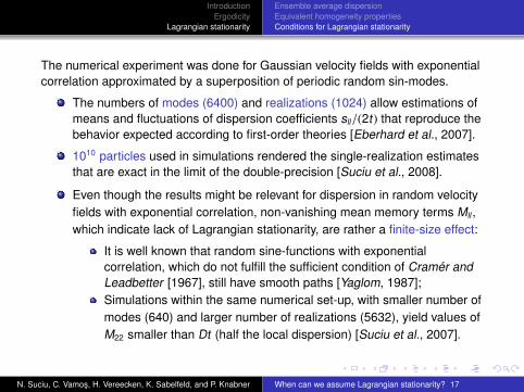
The numerical experiment was done for Gaussian velocity fields with exponentialcorrelation approximated by a superposition of periodic random sin-modes.

The numbers of modes (6400) and realizations (1024) allow estimations ofmeans and fluctuations of dispersion coefficients sll/(2t) that reproduce thebehavior expected according to first-order theories [Eberhard et al., 2007].

1010 particles used in simulations rendered the single-realization estimatesthat are exact in the limit of the double-precision [Suciu et al., 2008].

Even though the results might be relevant for dispersion in random velocityfields with exponential correlation, non-vanishing mean memory terms Mll ,which indicate lack of Lagrangian stationarity, are rather a finite-size effect:

It is well known that random sine-functions with exponentialcorrelation, which do not fulfill the sufficient condition of Cramer andLeadbetter [1967], still have smooth paths [Yaglom, 1987];Simulations within the same numerical set-up, with smaller number ofmodes (640) and larger number of realizations (5632), yield values ofM22 smaller than Dt (half the local dispersion) [Suciu et al., 2007].





Numerical estimations of the Lipschitz constant for single sin-mode with

exponential correlation (left) and for a superposition of 6400 sin-modes with

Gaussian correlation (right) indicate Lipschitz continuity, which is a necessary

condition in the proof of Lagrangian stationarity.





For a superposition of 6400 modes with exponential correlation, which generates

the samples of the velocity fields used in the numerical experiment, (left) the

Lipschitz constant behaves similarly with that of a sample of an almost

everywhere non-differentiable Wiener process (right).





Because the Lipschitz constant increases with the number of modes, it seemsthat the samples of the random velocity field with exponential correlation are notLipschitz continuous and the Lagrangian stationarity cannot be assumed.

Can the Lagrangian stationarity be proved under milder conditions?

For homogeneous velocity fields with small variance Σll − Sll(0) ≈ Xll andthe Lagrangian stationarity holds as a first-order approximation.





References

Conlon, J. G., and A. Naddaf (2000), Green’s functions for eliptic andparabolic equations with random coefficients, New York J. Math. 6, 153-225.

Cramer, H., and M. R. Leadbetter (1967), Stationary and Related StochasticProcesses, John Wiley & Sons, New York.

Dagan, G. (1990), Transport in heterogeneous porous formations: Spatialmoments, ergodicity and effective dispersion, Water Resour. Res., 26,1281–1290.

Dentz, M., and B. Berkowitz (2005), Exact effective transport inone-dimensional random environment, Phys. rev. E 72, 031110,doi:10.1103/PhysRevE.72.031110.

Eberhard J., N. Suciu, and C. Vamos (2007), On the self-averaging ofdispersion for transport in quasi-periodic random media, J. Phys. A: Math.Theor., 40, 597-610, doi: 10.1088/1751-8113/40/4/002.

Kitanidis, P. K. (1988), Prediction by the method of moments of transport ina heterogeneous formation, J. Hydrol., 102, 453–473.





References

Kloeden, P. E. and E, Platen (1995), Numerical Solutions of StochasticDifferential Equations, Springer, Berlin.

Kramer, P. R., and A. J. Majda (2007), Lectures on Turbulent Diffusion,Springer (in preparation).

Lumley, J. L. (1962), The mathematical nature of the problem of relatingLagrangian and Eulerian statistical functions in turbulence, pp , 17-26 inMecanique de la Turbulence, Ed. CNRS, Paris.

Sposito, G. and G. Dagan (1994), Predicting solute plume evolution inheterogeneous porous formations, Water Resour. Res., 30(2), 585–589.

Suciu N., C. Vamos, J. Vanderborght, H. Hardelauf, and H. Vereecken(2006), Numerical investigations on ergodicity of solute transport inheterogeneous aquifers, Water Resour. Res., 42, W04409,doi:10.1029/2005WR004546.

Suciu N., and C. Vamos (2007), Comment on “Nonstationary flow andnonergodic transport in random porous media” by G. Darvini and P.Salandin, Water Resour. Res., 43, W12601, doi:10.1029/2007WR005946.





References

Suciu, N., C. Vamos, K. Sabelfeld, and. C. Andronache (2007), Memoryeffects and ergodicity for diffusion in spatially correlated velocity fields, Proc.Appl. Math. Mech., 7, 2010015-2010016, doi:10.1002/pamm.20070057

Suciu N., C. Vamos, H. Vereecken, K. Sabelfeld, and P. Knabner (2008),Memory effects induced by dependence on initial conditions and ergodicityof transport in heterogeneous media, Water Resour. Res., 44, W08501,doi:10.1029/2007WR006740.

Suciu N., and P. Knabner (2009), Comment on “Spatial moments analysis ofkinetically sorbing solutes in aquifer with bimodal permeability distribution”by M. Massabo, A. Bellin, and A. J. Valocchi, Water Resour. Res., 45,doi:10.1029/2008WR007498, 2009 (in press).

Yaglom, A. M. (1987) Correlation Theory of Stationary and Related RandomFunctions, Volume I: Basic Results, Springer-Verlag, New York.

Zirbel, C., L. (2001), Lagrangian observations of homogeneous randomenvironments, Adv. Appl. Prob., 33, 810-835.





Acknowledgments

This study was supported by Deutsche Forschungsgemeinschaft grant SU415/1-2, Project JICG41 at Julich Supercomputing Centre, Romanian Ministry ofEducation and Research grant 2-CEx06-11-96, NATO Collaborative LinkageGrant ESP.NR.CLG 981426, and RFBR Grant 06-01-00498.

The authors gratefully acknowledge helpful private communications provided byJoseph Conlon, Peter Kramer, Orazgeldi Kurbanmuradov, Florin Radu, and

Craig Zirbel.





Thank you for your attention!


When can we assume Lagrangian stationarity?

Documents