Lecture 3: Lagrangian duality and algorithms for the ... · Lecture 3: Lagrangian duality and algorithms for the Lagrangian dual ... That the Lagrangian dual problem always is ...

Lecture 3: Lagrangian duality and

algorithms for the Lagrangian dual

problem

Michael Patriksson

0-0

1'

&

$

%

The Relaxation Theorem� Problem: find

f ∗ := infimumx

f(x), (1a)

subject to x ∈ S, (1b)

where f : Rn 7→ R given function, S ⊆ R

n

� A relaxation to (1) has the following form: find

f ∗R := infimum

x

fR(x), (2a)

subject to x ∈ SR, (2b)

where fR : Rn 7→ R is a function with fR ≤ f on S, and

SR ⊇ S

2'

&

$

%

� Relaxation Theorem: (a) [relaxation] f ∗R ≤ f ∗

(b) [infeasibility] If (2) is infeasible, then so is (1)

(c) [optimal relaxation] If the problem (2) has an

optimal solution, x∗R, for which it holds that

x∗R ∈ S and fR(x∗

R) = f(x∗R), (3)

then x∗R is an optimal solution to (1) as well

� Proof portion. For (c), note that

f(x∗R) = fR(x∗

R) ≤ fR(x) ≤ f(x), x ∈ S

� Applications: exterior penalty methods yield lower

bounds on f ∗; Lagrangian relaxation yields lower

bound on f ∗

3'

&

$

%

Lagrangian relaxation� Consider the optimization problem to find

f ∗ := infimumx

f(x), (4a)

subject to x ∈ X, (4b)

gi(x) ≤ 0, i = 1, . . . ,m, (4c)

where f : Rn 7→ R and gi : R

n 7→ R (i = 1, 2, . . . ,m) are

given functions, and X ⊆ Rn

� For this problem, we assume that

−∞ < f ∗ < ∞, (5)

that is, that f is bounded from below and that the

problem has at least one feasible solution

4'

&

$

%

� For a vector µ ∈ Rm, we define the Lagrange function

L(x,µ) := f(x) +m

∑

i=1

µigi(x) = f(x) + µTg(x) (6)

� We call the vector µ∗ ∈ Rm a Lagrange multiplier if it

is non-negative and if f ∗ = infx∈X L(x,µ∗) holds

5'

&

$

%

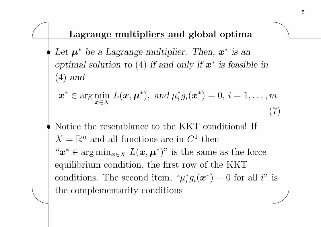
Lagrange multipliers and global optima� Let µ∗ be a Lagrange multiplier. Then, x∗ is an

optimal solution to (4) if and only if x∗ is feasible in

(4) and

x∗ ∈ arg minx∈X

L(x,µ∗), and µ∗i gi(x

∗) = 0, i = 1, . . . ,m

(7)

� Notice the resemblance to the KKT conditions! If

X = Rn and all functions are in C1 then

“x∗ ∈ arg minx∈X L(x,µ∗)” is the same as the force

equilibrium condition, the first row of the KKT

conditions. The second item, “µ∗i gi(x

∗) = 0 for all i” is

the complementarity conditions

6'

&

$

%

� Seems to imply that there is a hidden convexity

assumption here. Yes, there is. We show a Strong

Duality Theorem later

7'

&

$

%

The Lagrangian dual problem associated with the

Lagrangian relaxation

q(µ) := infimumx∈X

L(x,µ) (8)

is the Lagrangian dual function. The Lagrangian dual

problem is to

maximize

�

q(µ), (9a)

subject to µ ≥ 0m (9b)

For some µ, q(µ) = −∞ is possible; if this is true for all

µ ≥ 0m,

q∗ := supremum

� ≥0m

q(µ) = −∞

8'

&

$

%

� The effective domain of q is

Dq := { µ ∈ Rm | q(µ) > −∞}

� The effective domain Dq of q is convex, and q is

concave on Dq

� That the Lagrangian dual problem always is convex

(we indeed maximize a concave function!) is very good

news!

� But we need still to show how a Lagrangian dual

optimal solution can be used to generate a primal

optimal solution

9'

&

$

%

Weak Duality Theorem� Let x and µ be feasible in (4) and (9), respectively.

Then,

q(µ) ≤ f(x)

In particular,

q∗ ≤ f ∗

If q(µ) = f(x), then the pair (x,µ) is optimal in its

respective problem

10'

&

$

%

� Weak duality is also a consequence of the Relaxation

Theorem: For any µ ≥ 0m, let

S := X ∩ {x ∈ Rn | g(x) ≤ 0m }, (10a)

SR := X, (10b)

fR := L(µ, ·) (10c)

Apply the Relaxation Theorem

� If q∗ = f ∗, there is no duality gap. If there exists a

Lagrange multiplier vector, then by the weak duality

theorem, there is no duality gap. There may be cases

where no Lagrange multiplier exists even when there is

no duality gap; in that case, the Lagrangian dual

problem cannot have an optimal solution

11'

&

$

%

Global optimality conditions� The vector (x∗,µ∗) is a pair of optimal primal solution

and Lagrange multiplier if and only if

µ∗ ≥ 0m, (Dual feasibility) (11a)

x∗ ∈ arg minx∈X

L(x,µ∗), (Lagrangian optimality)

(11b)

x∗ ∈ X, g(x∗) ≤ 0m, (Primal feasibility) (11c)

µ∗i gi(x

∗) = 0, i = 1, . . . ,m (Complementary slackness)

(11d)

� If ∃(x∗,µ∗), equivalent to zero duality gap and

existence of Lagrange multipliers

12'

&

$

%

Saddle points� The vector (x∗,µ∗) is a pair of optimal primal solution

and Lagrange multiplier if and only if x∗ ∈ X,

µ∗ ≥ 0m, and (x∗,µ∗) is a saddle point of the

Lagrangian function on X × Rm+ , that is,

L(x∗,µ) ≤ L(x∗,µ∗) ≤ L(x,µ∗), (x,µ) ∈ X × Rm+ ,

(12)

holds

� If ∃(x∗,µ∗), equivalent to the global optimality

conditions, the existence of Lagrange multipliers, and a

zero duality gap

13'

&

$

%

Strong duality for convex programs, introduction� Results so far have been rather non-technical to

achieve: convexity of the dual problem comes with very

few assumptions on the original, primal problem, and

the characterization of the primal–dual set of optimal

solutions is simple and also quite easily established

� In order to establish strong duality, that is, to establish

sufficient conditions under which there is no duality

gap, however takes much more

� In particular, as is the case with the KKT conditions

we need regularity conditions (that is, constraint

qualifications), and we also need to utilize separation

theorems

14'

&

$

%

Strong duality Theorem� Consider problem (4), where f : R

n 7→ R and gi

(i = 1, . . . ,m) are convex and X ⊆ Rn is a convex set

� Introduce the following Slater condition:

∃x ∈ X with g(x) < 0m (13)

� Suppose that (5) and Slater’s CQ (13) hold for the

(convex) problem (4)

� (a) There is no duality gap and there exists at least one

Lagrange multiplier µ∗. Moreover, the set of Lagrange

multipliers is bounded and convex

15'

&

$

%

� (b) If the infimum in (4) is attained at some x∗, then

the pair (x∗,µ∗) satisfies the global optimality

conditions (11)

� (c) If the functions f and gi are in C1 then the

condition (11b) can be written as a variational

inequality. If further X is open (for example, X = Rn)

then the conditions (11) are the same as the KKT

conditions

� Similar statements for the case of also having linear

equality constraints.

� If all constraints are linear we can remove the Slater

condition

16'

&

$

%

Examples, I: An explicit, differentiable dual

problem� Consider the problem to

minimizex

f(x) := x21 + x2

2,

subject to x1 + x2 ≥ 4,

xj ≥ 0, j = 1, 2

� Let g(x) := −x1 − x2 + 4 and

X := { (x1, x2) | xj ≥ 0, j = 1, 2 }

17'

&

$

%

� The Lagrangian dual function is

q(µ) = minx∈X

L(x, µ) := f(x) − µ(x1 + x2 − 4)

= 4µ + minx∈X

{x21 + x2

2 − µx1 − µx2}

= 4µ + minx1≥0

{x21 − µx1} + min

x2≥0{x2

2 − µx2}, µ ≥ 0

� For a fixed µ ≥ 0, the minimum is attained at

x1(µ) = µ

2, x2(µ) = µ

2

� Substituting this expression into q(µ), we obtain that

q(µ) = f(x(µ)) − µ(x1(µ) + x2(µ) − 4) = 4µ − µ2

2

� Note that q is strictly concave, and it is differentiable

everywhere (due to the fact that f, g are differentiable

and x(µ) is unique)

18'

&

$

%

� We then have that q′(µ) = 4 − µ = 0 ⇐⇒ µ = 4. As

µ = 4 ≥ 0, it is the optimum in the dual problem!

µ∗ = 4;x∗ = (x1(µ∗), x2(µ

∗))T = (2, 2)T

� Also: f(x∗) = q(µ∗) = 8

� This is an example where the dual function is

differentiable. In this particular case, the optimum x∗

is also unique, and is automatically given by x∗ = x(µ)

19'

&

$

%

Examples, II: An implicit, non-differentiable dual

problem� Consider the linear programming problem to

minimizex

f(x) := −x1 − x2,

subject to 2x1 + 4x2 ≤ 3,

0 ≤ x1 ≤ 2,

0 ≤ x2 ≤ 1

� The optimal solution is x∗ = (3/2, 0)T, f(x∗) = −3/2

� Consider Lagrangian relaxing the first constraint,

20'

&

$

%

obtaining

L(x, µ) = −x1 − x2 + µ(2x1 + 4x2 − 3);

q(µ) = −3µ+ min0≤x1≤2

{(−1 + 2µ)x1}+ min0≤x2≤1

{(−1 + 4µ)x2}

=

−3 + 5µ, 0 ≤ µ ≤ 1/4,

−2 + µ, 1/4 ≤ µ ≤ 1/2,

− 3µ, 1/2 ≤ µ

� We have that µ∗ = 1/2, and hence q(µ∗) = −3/2. For

linear programs, we have strong duality, but how do we

obtain the optimal primal solution from µ∗? q is

non-differentiable at µ∗. We utilize the characterization

given in (11)

21'

&

$

%

� First, at µ∗, it is clear that X(µ∗) is the set

{(

2α

0

)

| 0 ≤ α ≤ 1 }. Among the subproblem solutions,

we next have to find one that is primal feasible as well

as complementary

� Primal feasibility means that

2 · 2α + 4 · 0 ≤ 3 ⇐⇒ α ≤ 3/4

� Further, complementarity means that

µ∗ · (2x∗1 + 4x∗

2 − 3) = 0 ⇐⇒ α = 3/4, since µ∗ 6= 0. We

conclude that the only primal vector x that satisfies

the system (11) together with the dual optimal solution

µ∗ = 1/2 is x∗ = (3/2, 0)T

� Observe finally that f ∗ = q∗

22'

&

$

%

� Why must µ∗ = 1/2? According to the global

optimality conditions, the optimal solution must in this

convex case be among the subproblem solutions. Since

x∗1 is not in one of the “corners” (it is between 0 and 2),

the value of µ∗ has to be such that the cost term for x1

in L(x, µ∗) is identically zero! That is, −1 + µ∗ · 2 = 0

implies that µ∗ = 1/2!

23'

&

$

%

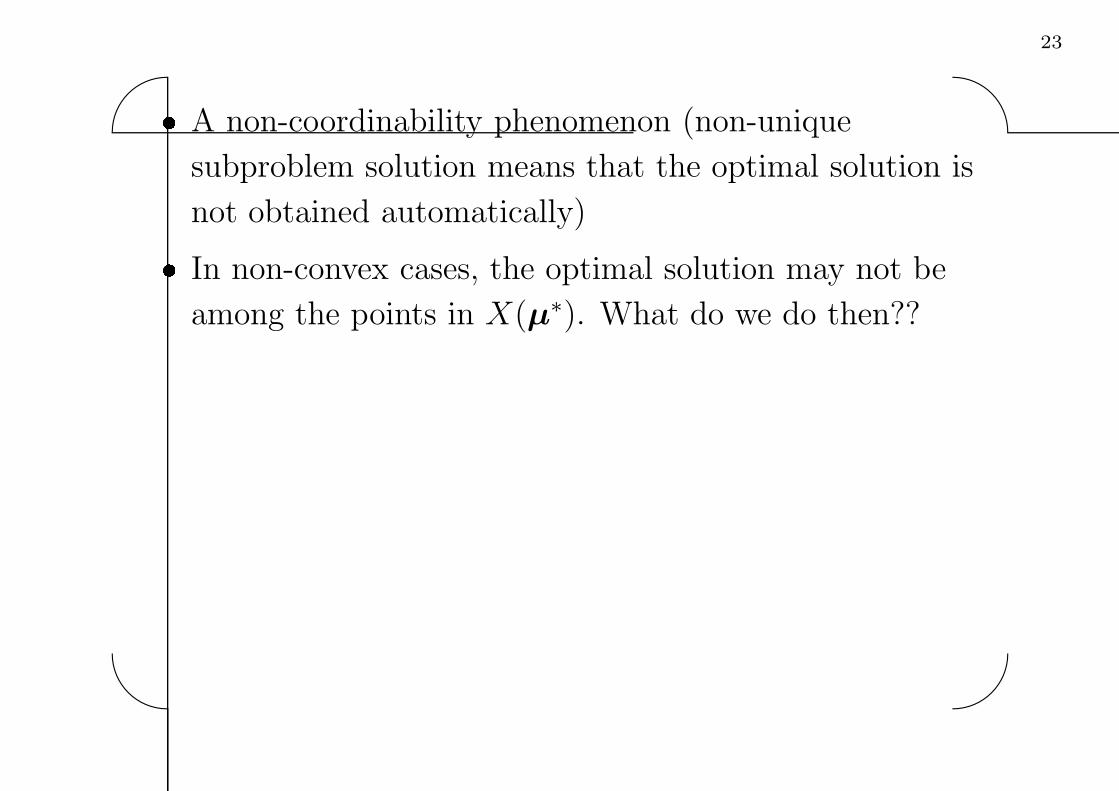
� A non-coordinability phenomenon (non-unique

subproblem solution means that the optimal solution is

not obtained automatically)

� In non-convex cases, the optimal solution may not be

among the points in X(µ∗). What do we do then??

24'

&

$

%

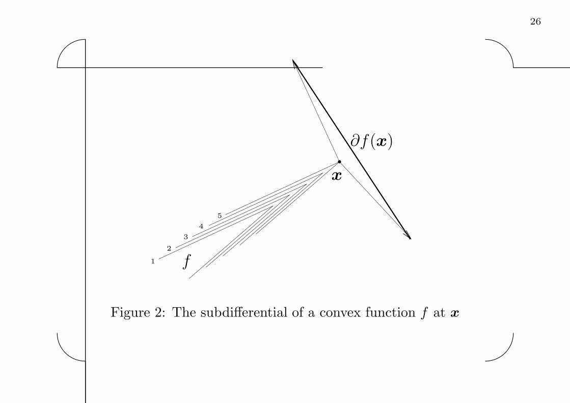
Subgradients of convex functions� Let f : R

n 7→ R be a convex function We say that a

vector p ∈ Rn is a subgradient of f at x ∈ R

n if

f(y) ≥ f(x) + pT(y − x), y ∈ Rn (14)

� The set of such vectors p defines the subdifferential of

f at x, and is denoted ∂f(x)

� This set is the collection of “slopes” of the function f

at x

� For every x ∈ Rn, ∂f(x) is a non-empty, convex, and

compact set

25'

&

$

%

PSfrag replacements

f

x

Figure 1: Four possible slopes of the convex function f at x

26'

&

$

%

PSfrag replacements

1

2

3

4

5

f

x

∂f(x)

Figure 2: The subdifferential of a convex function f at x

27'

&

$

%

� The convex function f is differentiable at x exactly

when there exists one and only one subgradient of f at

x, which then is the gradient of f at x, ∇f(x)

28'

&

$

%

Differentiability of the Lagrangian dual function:

Introduction� Consider the problem (4), under the assumption that

f, gi (i = 1, . . . ,m) continuous; X nonempty and compact

(15)

� Then, the set of solutions to the Lagrangian

subproblem,

X(µ) := arg minimumx∈X

L(x,µ), µ ∈ Rm, (16)

is non-empty and compact for every µ

� We develop the sub-differentiability properties of the

function q

29'

&

$

%

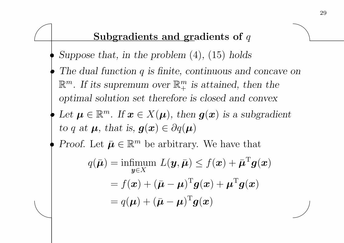
Subgradients and gradients of q� Suppose that, in the problem (4), (15) holds

� The dual function q is finite, continuous and concave on

Rm. If its supremum over R

m+ is attained, then the

optimal solution set therefore is closed and convex

� Let µ ∈ Rm. If x ∈ X(µ), then g(x) is a subgradient

to q at µ, that is, g(x) ∈ ∂q(µ)

� Proof. Let µ̄ ∈ Rm be arbitrary. We have that

q(µ̄) = infimumy∈X

L(y, µ̄) ≤ f(x) + µ̄Tg(x)

= f(x) + (µ̄ − µ)Tg(x) + µTg(x)

= q(µ) + (µ̄ − µ)Tg(x)

30'

&

$

%

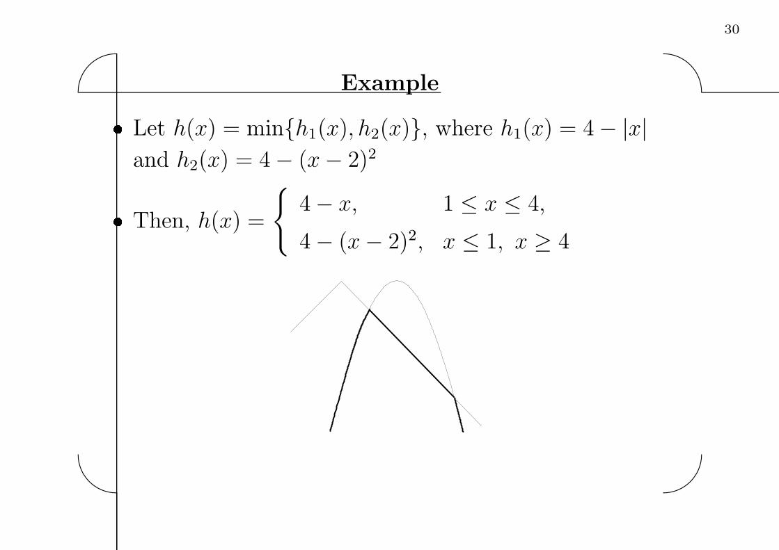
Example� Let h(x) = min{h1(x), h2(x)}, where h1(x) = 4 − |x|

and h2(x) = 4 − (x − 2)2

� Then, h(x) =

{

4 − x, 1 ≤ x ≤ 4,

4 − (x − 2)2, x ≤ 1, x ≥ 4

31'

&

$

%

� The function h is non-differentiable at x = 1 and x = 4,

since its graph has non-unique supporting hyperplanes

there

∂h(x) =

{−1}, 1 < x < 4

{4 − 2x}, x < 1, x > 4

[−1, 2] , x = 1

[−4,−1] , x = 4

� The subdifferential is here either a singleton (at

differentiable points) or an interval (at

non-differentiable points)

32'

&

$

%

The Lagrangian dual problem� Let µ ∈ R

m. Then, ∂q(µ) = conv { g(x) | x ∈ X(µ) }� Let µ ∈ R

m. The dual function q is differentiable at µ

if and only if { g(x) | x ∈ X(µ) } is a singleton set [the

vector of constraint functions is invariant over X(µ)].

Then,

∇q(µ) = g(x),

for every x ∈ X(µ)

� Holds in particular if the Lagrangian subproblem has a

unique solution [X(µ) is a singleton set]. In particular,

satisfied if X is convex, f is strictly convex on X, and

gi (i = 1, . . . ,m) are convex; q then even in C1

33'

&

$

%

� How do we write the subdifferential of h?� Theorem: If h(x) = mini=1,...,m hi(x), where each

function hi is concave and differentiable on Rn, then h

is a concave function on Rn

� Let I(x̄) ⊆ {1, . . . ,m} be defined by h(x̄) = hi(x̄) for

i ∈ I(x̄) and h(x̄) < hi(x̄) for i 6∈ I(x̄) (the active

segments at x̄)

� Then, the subdifferential ∂h(x̄) is the convex hull of

{∇hi(x̄) | i ∈ I(x̄)}, that is,

∂h(x̄)=

ξ=∑

i∈I(x̄)

λi∇hi(x̄)

∣

∣

∣

∣

∣

∣

∑

i∈I(x̄)

λi =1; λi ≥ 0, i ∈ I(x̄)

34'

&

$

%

Optimality conditions for the dual problem� For a differentiable, concave function h it holds that

x∗ ∈ arg maximumx∈ � n

h(x) ⇐⇒ ∇h(x∗) = 0n

� Theorem: Assume that h is concave on Rn. Then,

x∗ ∈ arg maximumx∈ � n

h(x) ⇐⇒ 0n ∈ ∂h(x∗)

� Proof. Suppose that 0n ∈ ∂h(x∗) =⇒

h(x) ≤ h(x∗) + (0n)T(x − x∗) for all x ∈ Rn, that is,

h(x) ≤ h(x∗) for all x ∈ Rn

Suppose that x∗ ∈ arg maximumx∈ � n h(x) =⇒

h(x) ≤ h(x∗) = h(x∗) + (0n)T(x − x∗) for all x ∈ Rn,

that is, 0n ∈ ∂h(x∗)

35'

&

$

%

� The example: 0 ∈ ∂h(1) =⇒ x∗ = 1� For optimization with constraints the KKT conditions

are generalized thus:

x∗ ∈ arg maximumx∈X

h(x) ⇐⇒ ∂h(x∗)∩NX(x∗) 6= ∅,

where NX(x∗) is the normal cone to X at x∗, that is,

the conical hull of the active constraints’ normals at x∗

36'

&

$

%

� In the case of the dual problem we have only sign

conditions� Consider the dual problem (9), and let µ∗ ≥ 0m. It is

then optimal in (9) if and only if there exists a

subgradient g ∈ ∂q(µ∗) for which the following holds:

g ≤ 0m; µ∗i gi = 0, i = 1, . . . ,m

� Compare with a one-dimensional max-problem (h

concave): x∗ is optimal if and only if

h′(x∗) ≤ 0; x∗ · h′(x∗) = 0; x∗ ≥ 0

37'

&

$

%

A subgradient method for the dual problem� Subgradient methods extend gradient projection

methods from the C1 to general convex (or, concave)

functions, generating a sequence of dual vectors in Rm+

using a single subgradient in each iteration

� The simplest type of iteration has the form

µk+1 = Proj�

m

+[µk + αkgk] (17a)

= [µk + αkgk]+ (17b)

= (maximum {0, (µk)i + αk(gk)i})mi=1, (17c)

where gk ∈ ∂q(µk) is arbitrarily chosen

38'

&

$

%

� We often use gk = g(xk), where

xk ∈ arg minimumx∈X L(x,µk)� Main difference to C1 case: an arbitrary subgradient gk

may not be an ascent direction!

� Cannot do line searches; must use predetermined step

lengths αk

� Suppose that µ ∈ Rm+ is not optimal in (9). Then, for

every optimal solution µ∗ ∈ U ∗ in (9),

‖µk+1 − µ∗‖ < ‖µk − µ∗‖

holds for every step length αk in the interval

αk ∈ (0, 2[q∗ − q(µk)]/‖gk‖2) (18)

39'

&

$

%

� Why? Let g ∈ ∂q(µ̄), and let U ∗ be the set of optimal

solutions to (9). Then,

U ∗ ⊆ {µ ∈ Rm | gT(µ − µ̄) ≥ 0 }

In other words, g defines a half-space that contains the

set of optimal solutions

� Good news: If the step length is small enough we get

closer to the set of optimal solutions!

40'

&

$

%

PSfrag replacements

1

2

3

4

5

q

g

µ

∂q(µ)

Figure 3: The half-space defined by the subgradient g of q at µ. Note

that the subgradient is not an ascent direction

41'

&

$

%

� Polyak step length rule:

σ ≤ αk ≤ 2[q∗ − q(µk)]/‖gk‖2 − σ, k = 1, 2, . . . (19)

� σ > 0 makes sure that we do not allow the step lengths

to converge to zero or a too large value

� Bad news: Utilizes knowledge of the optimal value q∗!

(Can be replaced by an upper bound on q∗ which is

updated)

� The divergent series step length rule:

αk > 0, k = 1, 2, . . . ; limk→∞

αk = 0;∞

∑

s=1

αs = +∞ (20)

42'

&

$

%

� Additional condition often added:∞

∑

s=1

α2s < +∞ (21)

43'

&

$

%

� Suppose that the problem (4) is feasible, and that (15)

and (13) hold� (a) Let {µk} be generated by the method (17), under

the Polyak step length rule (19), where σ is a small

positive number. Then, {µk} converges to an optimal

solution to (9)

� (b) Let {µk} be generated by the method (17), under

the divergent step length rule (20). Then,

{q(µk)} → q∗, and {distU∗(µk)} → 0

� (c) Let {µk} be generated by the method (17), under

the divergent step length rule (20), (21). Then, {µk}

converges to an optimal solution to (9)

44'

&

$

%

Application to the Lagrangian dual problem� Given µk ≥ 0m

� Solve the Lagrangian subproblem to minimize L(x,µk)

over x ∈ X

� Let an optimal solution to this problem be xk

� Calculate g(xk) ∈ ∂q(µk)

� Take a (positive) step in the direction of g(xk) from

µk, according to a step length rule

� Set any negative components of this vector to zero

� We have obtained µk+1

45'

&

$

%

Additional algorithms� We can choose the subgradient more carefully, such

that we will obtain ascent directions. This amounts to

gathering several subgradients at nearby points and

solving quadratic programming problems to find the

best convex combination of them (Bundle methods)

� Pre-multiply the subgradient obtained by some positive

definite matrix. We get methods similar to Newton

methods (Space dilation methods)

� Pre-project the subgradient vector (onto the tangent

cone of Rm+ ) so that the direction taken is a feasible

direction (Subgradient-projection methods)

46'

&

$

%

More to come� Discrete optimization: The size of the duality gap, and

the relation to the continuous relaxation.

Convexification

� Primal feasibility heuristics

� Global optimality conditions for discrete optimization

(and general problems)