Weibull Modulus Estimated by the Non-linear Least Squares ... · Weibull Modulus Estimated by the Non-linear Least Squares Method: A Solution to Deviation Occurring in Traditional

Weibull Modulus Estimated by the Non-linear LeastSquares Method: A Solution to Deviation Occurringin Traditional Weibull Estimation

T. LI, W.D. GRIFFITHS, and J. CHEN

The Maximum Likelihood method and the Linear Least Squares (LLS) method have beenwidely used to estimate Weibull parameters for reliability of brittle and metal materials. In thelast 30 years, many researchers focused on the bias of Weibull modulus estimation, and someimprovements have been achieved, especially in the case of the LLS method. However, there is ashortcoming in these methods for a specific type of data, where the lower tail deviatesdramatically from the well-known linear fit in a classic LLS Weibull analysis. This deviation canbe commonly found from the measured properties of materials, and previous applications of theLLS method on this kind of dataset present an unreliable linear regression. This deviation waspreviously thought to be due to physical flaws (i.e., defects) contained in materials. However,this paper demonstrates that this deviation can also be caused by the linear transformation ofthe Weibull function, occurring in the traditional LLS method. Accordingly, it may not beappropriate to carry out a Weibull analysis according to the linearized Weibull function, and theNon-linear Least Squares method (Non-LS) is instead recommended for the Weibull modulusestimation of casting properties.

DOI: 10.1007/s11661-017-4294-4� The Author(s) 2017. This article is an open access publication

I. INTRODUCTION

THE Weibull distribution has been widely used toanalyze the variability of the fracture properties ofbrittle materials for over 30 years. Fitting a Weibulldistribution also later became a popular method in theprediction of the quality and reproducibility of cast-ings.[1–3] The cumulative distribution function (CDF) ofthe Weibull distribution is given by[4]

P ¼ 1� exp � x� xux0

� �m� �; ½1�

where P is the probability of failure at a value of x, xu isthe minimum possible value of x, x0 is the probabilityscale parameter characterizing the value of x at which62.8 pct of the population of specimens have failed, andm is the shape parameter describing the variability in themeasured properties, which is also widely known as theWeibull moduli.

In a practical application, x could be substituted bythe symbol r for the properties of materials (e.g.,

Ultimate Tensile Strength (UTS)), and the lowestpossible value of property could be assumed to be 0,making xu = 0, so that Eq. [1] can be re-written as a2-parameter Weibull function:

P ¼ 1� exp � rr0

� �m� �: ½2�

There are several approaches to the estimation of theWeibull modulus in Eq. [2], with the most commonmethods being the Linear Least Squares method (LLS)and the Maximum Likelihood method (ML).Many researches focused on the bias of the estimated

Weibull modulus obtained by the estimation methods.Khalili and Kromp[5] recommended the ML and theLLS methods after a comparison of the ML, LLSmethods, and methods of momentum. Butikofer et al.[6]

found that the LLS method was less biased than the MLmethod for a small sample size. Tiryakioglu andHudak[7] and Wu et al.[8] studied the best estimatorsfor the LLS method.However, there is still a shortcoming in the LLS

method. In practice, some data points of the measuredproperties seriously deviate from the linear behavior inthe traditional LLS method for Weibull estimation,resulting in a bad fit in the linear regression model. Agood example was that of Griffiths and Lai’s[2] mea-surement of UTS of a commercial purity ‘‘top-filled’’

T. LI, W.D. GRIFFITHS, and J. CHEN are with the Universityof Birmingham, Birmingham B15 2TT, UK. Contact e-mail:[email protected]

Manuscript submitted December 22, 2016.Article published online August 24, 2017

5516—VOLUME 48A, NOVEMBER 2017 METALLURGICAL AND MATERIALS TRANSACTIONS A

Mg casting, as shown in Figure 1. It is clear that thedata points were not randomly scattered along the fittedstraight line in this linear regression, and the corre-sponding R2 value was only 79.1 pct, both of whichsuggested that it was a bad linear fit. These outlierswould exert much influence on the regression line,making the Weibull modulus deviate from its true value.This type of behavior (i.e., data deviation in the lowertail) in the plots of the linearized Weibull function(Figure 1) has occurred widely and resulted in estima-tion bias to various degrees, of which examples can befound in References 2 and 9 through 14. Keles et al.[14]

made a summary of this deviation occurring in themeasurement of brittle materials.

When this deviation occurs, a traditional solution isto firstly eliminate a few data points before the next stepof the Weibull moduli analysis,[1] because the datapoints in the lower tail were considered to be caused bygross pores. Nevertheless, the Weibull modulus obtainedafter such elimination would also neglect the effect ofporosity on the quality of the castings, and could notreflect the reproducibility of the whole castings.

Currently, a popular explanation for this deviation,based on a plot of linearized Weibull CDF (Figure 1), isthat the dataset may follow a 3-p/mixed Weibulldistribution.[15–17] The goodness-of-fit of linear regres-sion line (i.e., R2) was accordingly used to determine theWeibull behavior of the datasets.[18,19] Tiryakioglu[19]

developed the following equation for the critical R2

value to determine the Weibull behavior of a dataset:

R20:05 ¼ 1:0637� 0:4174

N0:3; ½3�

where R20:05 is the critical R

2 and N is the sample size. IfR2 of a linear regression was smaller than this criticalvalue, the corresponding dataset was thought to follow a3-p/mixed Weibull distribution.

This paper was aimed at investigating the reason forthis widely reported deviation, and finding an appropri-ate method to estimate the Weibull modulus when suchdeviations occur. Preliminary work demonstrated thatthe widely reported deviation can be also caused by the

linear transformation of the Weibull function, and aNon-LS method may be more appropriate to evaluatethe Weibull modulus. Comprehensive Monte Carlosimulations and a real casting experiment were subse-quently carried out to explore the reliability of theparameter estimation by Non-LS, LLS, and ML meth-ods. It has been shown that the Non-LS method, whichavoids the linear transformation, outperforms all theother methods.

II. BACKGROUND

A. Linear Least Squares (LLS) Methods

The Linear Least Squares method is also known asthe linear regression method. Taking the natural loga-rithm of Eq. [2] twice gives the linearized form of the 2-pWeibull CDF:

Ln �Ln 1� Pð Þ½ � ¼ mLn rð Þ �mLn r0ð Þ: ½4�

The Weibull modulus can then be determined accord-ing to the slope of a simple linear regression, (i.e.,ordinary least squares) of Ln [�Ln (1 � P)] againstLn(r), where the P value is assigned by a probabilityestimator. The probability estimators reported in theliterature were generally written in the form of

P ¼ i� a

Nþ b; ½5�

where i is the rank of the data sorted in an ascendingorder, N is the total sample size, a and b are constants,whose values depend on the estimators used. Thecommon estimators were summarized by Tiryakiogluand Hudak,[7] and are shown in Table I.

B. Maximum Likelihood (ML) Method

In statistics, the likelihood is a function of theparameters of a given observed dataset and the under-lying statistical model. ‘‘Likelihood’’ is related to, but isnot equivalent to ‘‘probability’’; the former is used afterthe outcome data are available to describe that some-thing that is likely to have happened, while the latterdescribes possible future outcomes before the data areavailable.

Fig. 1—Weibull estimation using the LLS method, which was pub-lished in Ref. [2] (the ‘‘Top-filled’’ results).

Table I. Probability Estimators Summarized by Ref. [6]

a b

0.5 0 Eq. [6]0 1 Eq. [7]0.3 0.4 Eq. [8]0.375 0.250 Eq. [9]0.44 0.12 Eq. [10]0.25 0.50 Eq. [11]0.4 0.2 Eq. [12]0.333 0.333 Eq. [13]0.50 0.25 Eq. [14]0.31 0.38 Eq. [15]

METALLURGICAL AND MATERIALS TRANSACTIONS A VOLUME 48A, NOVEMBER 2017—5517

The basic principles can be described as follows.[20–22]

If there is a dataset of N independent and identicallydistributed observations, namely x1, x2,…, xN, comingfrom a underlying probability density function f(h). Thetrue value of h is unknown and it is desirable to find an

estimator h which would be as close to htrue as possible.First the joint density function for all observations canbe calculated as

f x1x2 . . . xnjhð Þ ¼ f x1jhð Þf x2jhð Þ � � � � f xnjhð Þ ¼Yni¼1

f xijhð Þ:

½16�

From a different perspective, Eq. [16] can be consid-ered to have the observed data x1, x2,…, xN, as the fixedparameters and h as the function’s variable. This will becalled the likelihood function as follows

L hjx1x2 . . . xnð Þ ¼ f x1x2 . . . xnjhð Þ ¼Yni¼1

f xijhð Þ: ½17�

The maximum likelihood estimate (MLE) of h can beobtained by maximizing the likelihood function giventhe observed data as

hMLE ¼ argmaxh

L hjx1x2 . . . xnð Þ: ½18�

For a Weibull estimation of castings, the likelihoodfunction of the observed dataset, x1, x2,…, xN, can bewritten as

L m; rjx1; x2; . . . ; xNð Þ ¼YNi¼1

fðxijm; rÞ

¼YNi¼1

m

rx

r

� �m�1

exp � xir

� �m� �� �:

½19�

Here f(xiŒm, r) is the probability density function ofWeibull distribution. MLE of a Weibull parameter canbe then obtained by maximizing Eq. [19], usingNelder–Mead method.

The estimated Weibull modulus obtained by theMaximum Likelihood method was also biased fromthe value of mtrue. Khalili[5] reported that the bias levelof the ML Method was higher than Eq. [6] of the linearleast square method. This suggestion was also supportedby the following study of References 6 and 8.

C. Non-linear Least Squares (Non-LS) Method

The Non-LS method has many similarities to the LLSmethod. The observed data are also sorted in anascending fashion, and subsequently paired with thefailure probabilities, obtained by the estimators shownin Table I. It differs from the LLS method as anon-linear regression, using a Gauss–Newton algorithm,is directly carried out to achieve the best fitted curve of aWeibull function. This method was used to estimate

Weibull parameters in some other fields,[23,24] but hasnot been applied in the Weibull estimation of castingsand brittle materials.

III. METHODS

A. Re-analysis of Griffiths and Lai’s Data

As shown in Figure 2, the Griffiths’ data shown inFigure 1 (i.e., UTS of a commercial purity Mg castingproduced using a top-filled running system) were re-an-alyzed using the Non-LS method. To compare the fittingperformance, the Weibull function with the parametersobtained by the LLS method (i.e., the method originallyused in Griffiths and Lai’s paper[2]) is also plotted inFigure 2. Residual Sum of Squares (SSR) was used toevaluate the goodness-of-fit instead of R2 in this non-lin-ear model (the adjusted R2 values were also given).According to Figure 2(a), it can be seen that the data

points showed a good fit to the Non-linear regressioncurve (SSR = 0.0238), which is much better than thecurve plotted according to the LLS estimation results(the Weibull parameters shown in Figure 1, SSR =0.4096). There was a significant difference between theWeibull modulus estimated by the two methods (11.147and 4.427). Therefore, although the Tiryakioglu’s equa-tion (i.e., Eq. [3], (R0.05)

2 = 0.9047) rejected the Weibullbehavior of this dataset, it is still not clear whether thedata points follow a 2-p Weibull distribution.According to Figure 2(b), when the Non-LS estima-

tion result was plotted in the linearized Weibull plot(i.e., solid line in Figure 2(b)), the data points showed avery bad fit to the line (R2<0), which was much worsethan the LLS estimation results (R2 = 79.1 pct). Thecontradictory conclusions of Figures 2(a) and (b) sug-gest the following question: ‘‘Is it appropriate todetermine the Weibull behavior of datasets accordingto the traditional linearized Weibull plot (Figure 2(b)),or the non-linear Weibull plot (Figure 2(a))?’’

B. A Shortcoming of the Linearized Form of the WeibullFunction

It should be noted that according to the estimatordefined as Eq. [5], the cumulative probability in theWeibull estimation using the least square method is set toa specific value (denoted by Pest,i for the ith datum point)with the same weight for each datum point. However, ina practical process, the true cumulative probability,referred to as Ptrue,i, is of course not necessarily equal tothe estimated cumulative probability (Pest,i). Bergman[25]

also pointed out that it was erroneous to assume thesame weight for each datum point in Eq. [5]. Thus, thereis usually a difference between Ptrue,i and Pest,i, makingthe estimated Weibull moduli biased.Let DYnon-linear,i indicate the difference between the

true and estimated values on the Y axis for the ith datumpoint in the plot of the original Weibull CDF, as shownin the following equation:

DYnon�linear;i ¼ Ptrue;i � Pest;i

�� ��: ½20�

5518—VOLUME 48A, NOVEMBER 2017 METALLURGICAL AND MATERIALS TRANSACTIONS A

Similarly, let DYlinear,i indicate this difference on theY axis in the plot of the linearized Weibull function(Eq. [3]), which can be calculated by the followingequation:

DYlinear;i ¼ Ln½�Lnð1� Ptrue;iÞ� � Ln½�Lnð1� Pest;iÞ��� ��:

½21�

As shown in Figure 3, no matter how much Ptrue,i andPest,i are, linear transformation can always numericallyenlarge the difference between the true and estimatedvalues on the Y axis. In other words, DYlinear,i is alwayslarger than DYnon-linear,i, especially when Pest,i signifi-cantly deviates from Ptrue,i. Such an increase, in the

deviation from the estimated value to the true value onthe Y axis, causes a larger distance between theestimated and true positions of the data points in thelinearized Weibull function plot, compared with that inthe original Weibull CDF plot. Furthermore, it shouldbe noted that the enlargement due to the lineartransformation also exists in the linearized form of the3-p Weibull function.This enlargement level can be further described by the

following enlargement factor (EF):

Enlargement factor: EF ¼ DYnon�linear;i

DYlinear;i: ½22�

A 3D plot of this equation is shown in Figure 4. It canbe seen that the EF value would be significantly small,

Fig. 2—(a) Weibull estimation of Griffiths’ data shown in Fig. 1, using the Non-LS method and the LLS method. The used estimator is P =(i � 0.5)/N (Eq. [6] shown in Table I). (b) The results of the two methods plotted in the plot of the linearized Weibull function.

Fig. 3—(a) A 3D plot based on the functions of DYlinear,i and DYnon-linear,i. (b) View from another direction of (a), indicating that DYlinear,i isalways larger than DYnon-linear,i.

METALLURGICAL AND MATERIALS TRANSACTIONS A VOLUME 48A, NOVEMBER 2017—5519

even close to 0, when Ptrue,i approaches to 0 or 1, whichmeans that the DYnon-linear,i would be dramaticallyenlarged at these positions. This non-uniform enlarge-ment is the underlying reason why it was normal toreport a deviation in the lower and upper tails of adataset in a traditional linearized Weibull plot(Figure 1).

Since the regression algorithms of the least squaremethod (no matter linear or non-linear regression)produce the result according to the residuals (i.e., thesmallest Sum of Residual Squares), which is only relatedto the Y-coordinate, the non-uniform enlargement ofDYlinear,i accordingly may result in more bias of theregression results (such as the estimated Weibull mod-uli). Therefore, the bad fit of the Non-LS estimationresult shown in Figure 4(b) may be due to the enlarge-ment of the difference between the true and estimatedprobabilities. The least square method has been accord-ingly used in this paper in the plot of the non-linearWeibull CDF, rather than its linearized form. Thisapproach is the non-linear least square method(Non-LS).

C. Examples of the Negative Effect of the Enlargementof DYnon-linear,i on Weibull Estimation

For a further illustration of the negative effect of theenlargement of DYnon-linear,i, an example has been givenin Table II. This dataset was generated from a 2-pWeibull distribution with shape = 11 and scale= 60,which was close to the Non-LS estimation result ofGriffiths (Figure 1). The raw data were sorted inascending order, shown in the second column ofTable II. The true cumulative probabilities (Ptrue,i) weredirectly calculated from the Weibull function as listed inthe third column. The estimated cumulative probabilitywas computed according to Pest,i = (i � 0.5)/N (Eq. [6]),

and has been shown in the 4th column. DYlinear,i andDYnon-linear,i were listed in the 5th and 6th columns,respectively.Figures 5(a) and (b) show the corresponding Weibull

estimation results using the Non-LS and LLS methods.The solid square points indicate Ptrue,i, while the hollowtriangle points denote Pest,i. It can be seen that thedeviation from the estimated value to the true value onthe Y axis was obviously larger in the plot of thelinearized Weibull function (DYlinear,i in Figure 5(b)),than in the plot of the original non-linear Weibull CDF(DYnon-linear,i in Figure 5(a)), especially when Ptrue,i issmall. A deviation similar to that shown in Figure 1 (i.e.,Griffiths’ data) consequently occurred in the lower tailas shown in Figure 5(b).In addition, the Weibull behavior of this dataset was

also rejected by Tiryakioglu’s equation (Eq. [3]). Theline plotted based on the Non-LS estimation (i.e., thesolid black line in Figure 5(b)) showed an extreme badfit to the triangle points (i.e., R2< 0), similar to thatshown in Figure 2(b). However, this line was more closeto the true function than the linear regression line.Figure 5(c) shows the change in the enlargement

factor (EF) along with Ptrue,i, revealing that the enlarge-ment of DYnon-linear,i was more dramatic when Ptrue,i isclose to 0 and 1, which is consistent with Figure 4.Accordingly, the performance of the Weibull moduliestimation is poorer in the LLS method than in theNon-LS method, which can explain the different level ofthe goodness-of-fit in different Weibull plots as shown inFigure 2.

IV. SIMULATION PROCEDURES

To further illustrate the discussion in Section III,Monte Carlo simulations were performed in R Version

Fig. 4—(a) The function of the enlargement factor (EF). (b) View from another direction of (a), indicating the DYnon-linear,i would be dramati-cally enlarged when Pture,i is close to 0 or 1.

5520—VOLUME 48A, NOVEMBER 2017 METALLURGICAL AND MATERIALS TRANSACTIONS A

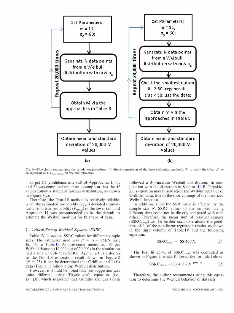
3.3.0 (https://www.r-project.org). As shown in Figure 6,different procedures were used to investigate the bias ofthe estimated Weibull modulus.

For direct comparison of the different estimationmethods (Figure 6(a)), random data points of samplesize N were firstly generated from a 2-p Weibull function(Eq. [2]) with shape parameter =11 (referred to as mtrue)and scale parameter = 60 (referred to as r0,true). Thedifferent approaches, listed in Table III, were used toevaluate the Weibull modulus (written as mest) of thegenerated data.

The bias of the estimated Weibull modulus (mest) wasdefined by the following equation,[5,7,26]

M ¼ mest=mtrue: ½23�

M = 1 means the approach used was unbiased. Inaddition, since the estimated parameters are normalizedby the true parameters, the setting of the scale and shapeparameters are inconsequential.[5,19] This process wasrepeated for 20,000 times to obtain 20,000 M values.The bias level of the different approaches was evaluatedby the mean of the 20,000 M values, written as Mmean.

To study the effect of the dramatic enlargement ofDYnon-linear,i on Weibull moduli estimation(Figure 6(b)), the program checked whether the smallestdatum of the randomly generated dataset was<30, thusmaking the data used for the simulation contain at leastone datum point smaller than 30. This setting ensured asmall value of the true probability of the first datumpoint (Pture,1), and thus the corresponding differencebetween the true and estimated values on the Y axis(DYnon-linear,1) would be dramatically enlarged in the

linearized Weibull function plot, according to Figure 4(when Ptrue,1 is close to 0).Based on the linearized Weibull plot, Tiryakioglu

et al.[19] developed an equation for critical R2 (seeEq. [3]), to determine the Weibull behavior of datasets.Similarly, based on the non-linear Weibull plot, thecritical SSR (referred to as SSRC) could also becalculated using a Monte Carlo simulation and theprocedures shown in Figure 6(c). The SSRC obtainedwould be larger than the SSR value of 95 pct datasets(i.e., 19,000 out of 20,000).

V. RESULTS

A. Direct Comparison of the Estimation Approaches

Figure 7 illustrates the results of the simulationsshown in Figure 6(a). In general, the estimated Weibullmodulus became closer to mtrue with increase in samplesize N. Figure 7(a) summarizes the Mmean obtained bythe LLS and the ML methods (i.e., Approaches 1 to 10and 21 in Table III). It can be seen that Approaches 1and 9 were relatively less biased for N ‡ 25, andApproach 5 was the least biased approach when thesample size N was<25. This observation was consistentwith the results of References 5 and 7. Figure 7(b) showsa summary of Mmean achieved via the Non-LS method(i.e., Approaches 11 to 20 in Table III). It was obviousthat Approach 12, which was the worst estimator for theLLS method (i.e., Approach 2), was less biased than theother estimators using the Non-LS method, especiallywhen the sample size was smaller than 30.

Table II. Data (Referred to as x) Generated from a Weibull Function with Shape = 11, Scale = 60

i x Ptrue,i Pest,i = (i � 0.5)/N DYlinear,i DYnon-linear,i

1 34.0085 0.001938 0.02 0.018062 2.343142 34.6850 0.002406 0.06 0.057594 3.245763 37.1551 0.005122 0.10 0.094878 3.021304 42.4875 0.022199 0.14 0.117801 1.904845 51.1540 0.158850 0.18 0.021150 0.137346 51.8391 0.181473 0.22 0.038527 0.215737 54.0502 0.271693 0.26 0.011693 0.051558 54.5408 0.295427 0.30 0.004573 0.018439 55.1336 0.325901 0.34 0.014099 0.0522110 55.2120 0.330076 0.38 0.049924 0.1767411 55.3406 0.336997 0.42 0.083003 0.2817512 55.7049 0.357082 0.46 0.102918 0.3328313 56.6743 0.413777 0.50 0.086223 0.2607414 57.0168 0.434843 0.54 0.105157 0.3080515 57.8910 0.490647 0.58 0.089353 0.2514816 58.0565 0.501496 0.62 0.118504 0.3292517 58.2651 0.515268 0.66 0.144732 0.3986018 58.6562 0.541344 0.70 0.158656 0.4347919 59.7578 0.615759 0.74 0.124241 0.3424220 60.5805 0.671011 0.78 0.108989 0.3089221 60.8124 0.686338 0.82 0.133662 0.3913622 61.0008 0.698679 0.86 0.161321 0.4940923 62.7504 0.805486 0.90 0.094514 0.3410124 63.0698 0.822946 0.94 0.117054 0.4855225 64.0881 0.873164 0.98 0.106836 0.63899

METALLURGICAL AND MATERIALS TRANSACTIONS A VOLUME 48A, NOVEMBER 2017—5521

For a further comparison, Approaches 1, 5, 9, and 12were put together as shown in Figure 7(c). For 15 £ N<35 and 90 £ N, it was clear that Approach 12 resulted inthe least bias for all the sample sizes. For 35 £ N< 90,Approaches 1 and 12 were better than the otherapproaches. Figure 7(d) shows the Standard Error(SE) of M, revealing a negligible difference betweenthe SE values of different approaches.

B. Effect of a Dramatic Enlargement of DYnon-linear,i

Figure 8 shows the Mmean of the datasets containingat least one datum point <30. As can be seen fromFigure 8(a), the LLS method (i.e., Approaches 1 to 10 inTable III) was seriously biased when dealing with thistype of data. For 15 £ N £ 40, which was the commonsample size for obtaining the Weibull modulus ofcastings in previous publications,[2,27–29] the Mmean

values were no more than 0.7, presenting a significantbias of the estimated Weibull modulus. In addition, evenwith a large sample size, such as N = 115, the Mmean

values of Approaches 1 to 10 still did not exceed 0.85.Thus, it can be suggested that the LLS method is notsuitable for estimating the Weibull modulus, when Pest.i

dramatically deviates from Ptrue,i in the lower tail. Thismay explain why the data points shown in Figure 1deviated from the linear fit.By contrast, according to Figure 8(b), the Non-LS

method (i.e., Approaches 11 to 20) was significantly lessbiased. Even the worst approach (Approach 12) of theNon-LS method could cause a smaller bias (Mmean >0.85, at N =15) than any approaches using the LLSmethod (Mmean < 0.8, at N = 115). In addition,Approach 11 obtained the least biased estimates amongall the approaches using the Non-LS methods (Ap-proaches 11 to 20), especially when the sample size wassmaller than 30.Moreover, it should be noted that Approach 12,

which was unbiased in Figure 7(b), became the mostseriously biased estimator among the approaches of theNon-LS method, indicating that the bias of theapproaches could be different depending on the levelof the enlargement of DYnon-linear,i.Mmean obtained by the ML method (Approach 21 in

Table III) was also shown in Figure 8(b), but it wasclear that Approach 21 was more biased for all thesample sizes examined, in contrast to the Non-LSmethod.

Fig. 5—(a) and (b) Weibull estimation using (a) the Non-LS and (b) LLS methods, corresponding to the data listed in Table II. The black pointsindicate Ptrue,i, while the red points denote Pest,i. (c) The change of EF along with Pture,i.

5522—VOLUME 48A, NOVEMBER 2017 METALLURGICAL AND MATERIALS TRANSACTIONS A

95 pct CI (confidence interval) of Approaches 1, 11,and 21 was computed under an assumption that the Mvalues follow a standard normal distribution, as shownin Figure 8(c).

Therefore, the Non-LS method is relatively reliable,when the estimated probability (Pest.i) deviated dramat-ically from true probability (Pture,i) in the lower tail, andApproach 11 was recommended to be the default toestimate the Weibull modulus for this type of data.

C. Critical Sum of Residual Squares (SSRC)

Table IV shows the SSRC values for different samplesizes. The estimator used was P = (i � 0.5)/N (i.e.,Eq. [6] in Table I). As previously mentioned, 95 pctWeibull datasets (19,000 out of 20,000) in the simulationhad a smaller SSR than SSRC. Applying this criterionto the Non-LS estimation result shown in Figure 2(N = 25), it can be determined that Griffiths and Lar’sdata (Figure 1) follow a 2-p Weibull distribution.

However, it should be noted that this suggestion wasquite different using Tiryakioglu’s equation (i.e.,Eq. [3]), which suggested that Griffiths and Lar’s data

followed a 3-p/mixture Weibull distribution. In con-junction with the discussion in Section III–B, Tiryakio-glu’s equation may falsely reject the Weibull behavior ofGriffiths’ data, due to the shortcomings of the linearizedWeibull function.In addition, since the SSR value is affected by the

sample size N, SSRC values of the samples havingdifferent sizes could not be directly compared with eachother. Therefore, the mean sum of residual squares(SSRCmean) can be further used to evaluate the good-ness-of-fit of the non-linear regression results, as shownin the third column of Table IV and the followingequation:

SSRCmean ¼ SSRC=N: ½24�

The best fit curve of SSRCmean was computed asshown in Figure 9, which followed the formula below:

SSRCmean ¼ 0:06463 �N�0:93778: ½25�

Therefore, the author recommends using this equa-tion to determine the Weibull behavior of datasets.

Fig. 6—Flowcharts summarizing the simulation procedures: (a) direct comparison of the three estimation methods; (b) to study the effect of theenlargement of DYnon-linear,i on Weibull estimation.

METALLURGICAL AND MATERIALS TRANSACTIONS A VOLUME 48A, NOVEMBER 2017—5523

D. Practical Data from Mg-Alloy Castings

Figure 10 shows an example of a commercial purityMg-alloy casting. Similar to the casting shown inFigure 1, this Mg casting was also produced using aresin-bonded sand mold with a top-filled system, and thecasting procedures were the same as Griffiths and Lai’swork.[2] The material used was from the same batch as

the Mg alloy used by Griffiths and Lai,[2] so it can bereadily compared. Thus, the reproducibility of thiscasting was expected to be close to the results from thecasting shown in Figure 1. After solidification, thecasting was machined into 40 test bars and tensilestrength was tested. The UTS data were used forWeibull analysis.

Table III. Approaches Using the Estimators Shown in Table I Together with LLS, Non-LS, and ML Methods

Estimators

Methods

LLS Non-LS ML

Eq. [6] Approach 1 Approach 11 Approach 21Eq. [7] Approach 2 Approach 12Eq. [8] Approach 3 Approach 13Eq. [9] Approach 4 Approach 14Eq. [10] Approach 5 Approach 15Eq. [11] Approach 6 Approach 16Eq. [12] Approach 7 Approach 17Eq. [13] Approach 8 Approach 18Eq. [14] Approach 9 Approach 19Eq. [15] Approach 10 Approach 20

Fig. 7—Mmean values obtained via the approaches in Table III, (a) Approaches 1 to 10 and 21, (b) Approaches 11 to 20, for a direct comparisonof the three estimation methods; (c) a further comparison of Approaches 1, 5, 9, and 12 shown in (a) and (b); (d) Standard Error (SE) of the ap-proaches shown in (a) and (b).

5524—VOLUME 48A, NOVEMBER 2017 METALLURGICAL AND MATERIALS TRANSACTIONS A

Figure 10 shows the Weibull parameters evaluatedusing Approaches 1 and 11. It can be seen that the datapoints showed a good fit to the linear regression line(Figure 10(a)). In addition, in Figure 10(b), the datapoints showed a good fit to both the curves obtainedusing the Non-LS method (Approach 11, SSR =0.0222) and the LLS method (Approach 1, SSR =0.0265). In conjunction with Figure 7, the enlargementof DYnon-linear,i in the dataset may not be dramatic. Theestimated Weibull moduli (11.7 and 11.4) were close tothe Non-LS estimation results shown in Figure 1, ratherthan the LLS estimation results.

As previously mentioned, this casting process (i.e., thecasting shown in Figure 10) is the same as the Griffithsand Lai’s casting process (i.e., the casting shown inFigure 2), and thus the estimated Weibull modulusshown in Figure 10 should be close to the true Weibullmodulus of Griffiths and Lai’s casting. Therefore, theWeibull modulus shown in Figure 10 could be used asthe reference value to determine which Weibull modulus(i.e., the LLS and Non-LS estimation results) inFigure 2 was closer to the true value. Based on thecomparison between Figures 2 and 10, it can be

suggested that the Non-LS estimation result shown inFigure 2 (i.e., m = 11.14) is closer to the true Weibullmodulus than the LLS estimation result (i.e., m = 4.4).The Non-LS method is accordingly more appropriate toestimate the Weibull modulus of Griffiths and Lai’sdata.In addition, this comparison (Figures 10 and 2)

further revealed that the SSRC method (Figure 9) maybe more appropriate to interpret Griffiths and Lai’sdata, while Tiryakioglu’s equation (Eq. [3]) will falselyinterpret this dataset to be a 3-p Weibull distribution.Figure 11 shows an example of results from an AZ91

casting, produced in the same way as the cast test barresults shown in Figure 10. As shown in Figure 11(a),the data points deviated from the linear regression line,and the corresponding R2 was smaller than the criticalR2 suggested by Eq. [3] [(R0.05)

2 = 0.9256), rejecting theWeibull behavior of this dataset. However, according tothe non-linear Weibull plot (Figure 11(b)], there was aclear difference between curves obtained by Approaches1 (the LLS method) and 11 (the Non-LS method). Thecurves obtained by Approach 11 have an SSR valuesmaller than the critical SSR (SSRC = 0.0816979,

Fig. 8—Mmean of Approaches (a) 1 to 10 and (b) 11 to 21 applied on the dataset containing at least one datum<30. (c) 95 pct CI of Approaches1, 11, 21 applied on dataset containing at least one datum<30. (d) Standard error of M.

METALLURGICAL AND MATERIALS TRANSACTIONS A VOLUME 48A, NOVEMBER 2017—5525

Table IV), suggesting the data followed a 2-p Weibulldistribution. This different judgment of Weibull behav-ior is similar to that found in the estimation of Griffithsand Lai’s data (Figure 2), and the dataset may be falselyinterpreted in the linearized Weibull plot.

VI. DISCUSSION

A. Determination of Weibull Behavior of Datasets

Figure 3 indicates that the difference between theestimated and true cumulative probabilities of datapoints (DYnon-linear,i) would be significantly enlarged dueto the linear transformation of the Weibull function.Figure 4 further reveals that this enlargement level wasnot uniform: the enlargement could be more dramatic inthe lower and upper tails (i.e., when Ptrue,i is close to 0or 1).

According to the Weibull analysis of example data(Figures 2 and 5), the non-uniform enlargement ofDYnon-linear,i can affect the judgement of the Weibullbehavior of datasets. The re-analysis of Griffiths’ data(Figure 2) and the corresponding SSRC value(Table IV) indicated that it may not be necessarilycorrect to reject the Weibull behavior of datasets,according to the goodness-of-fit of the linear regressionline (Eq. [3]). It should be noted that if a significantenlargement of DYnon-linear,i occurred in the lower tail(i.e., the first few data points), even a dataset generatedfrom a Weibull distribution would probably present abad fit to the linear regression line, as shown inFigure 5(b).

The experimental result (Figure 10) further showedthe dataset of a top-filled commercial purity Mg castingfollowed a 2-p Weibull distribution, according to bothR2 and SSR. In addition, both of the LLS and Non-LSresults in Figure 10 were close to the Non-LS estimationresult of Griffiths and Lai (Figure 2), which furthersupported the reliability of the Non-LS estimation.Figure 11 shows a further example that the dataset maybe falsely interpreted.Therefore, the non-uniform enlargement of

DYnon-linear,i is an underlying reason for the deviationof the data points widely found in previous publica-tions.[2,9–13] Previous researchers suggested that thisdeviation could be due to the nature of the physicalflaws (i.e., defects, such as porosity, low melting pointintermetallic compounds, and segregation) in the mate-rial,[14,30] and the corresponding data points wereinterpreted to follow an underlying 3-p or mixedWeibull distribution.[15–17] However, more analysis(Eq. [25]) is still required to distinguish what is theactual reason of the deviation. The simulation results(Figure 5) and experimental results (Figures 2 and 10)indicated that a deviation caused by the non-uniformenlargement of DYnon-linear,i could be falsely interpretedto be due to physical flaws (i.e., 3-p/mixed Weibulldistribution). This misunderstanding may exist in pre-vious researches.

B. Effect of Weibull Modulus Estimation

The results of the Monte Carlo simulations demon-strated that the non-uniform enlargement ofDYnon-linear,i resulted in a greater bias in the Weibullmodulus estimation. When the difference betweenDYlinear,i and DYnon-linear,i was not necessarily large(Figure 7), the Non-LS method was slightly less biasedthan the LLS method. However, when high enlargementof DYnon-linear,i occurs in the lower tail (Figure 5), theNon-LS method has a considerable merit over the LLSmethod.It is therefore recommended that the plot of the

original non-linear Weibull CDF and the Non-LS

Table IV. SSRC Values; the Estimator Used is P =

(i 2 0.5)/N

N SSRC SSRCmean

15 0.0756771 5.0451E�0320 0.0784904 3.9245E�0325 0.0797666 3.1907E�0330 0.0802094 2.6736E�0335 0.0818855 2.3396E�0340 0.0816979 2.0424E�0345 0.0832347 1.8497E�0350 0.0826510 1.6530E�0355 0.0837245 1.5223E�0360 0.0829798 1.3830E�0365 0.0834890 1.2844E�0370 0.0831899 1.1884E�0375 0.0844495 1.1260E�0380 0.0846093 1.0576E�0385 0.0842047 9.9064E�0490 0.0849502 9.4389E�0495 0.0840484 8.8472E�04100 0.0846551 8.4655E�04105 0.0833319 7.9364E�04110 0.0842549 7.6595E�04115 0.0845723 7.3541E�04120 0.0838167 6.9847E�04

Fig. 9—SSRCmean for different sample sizes.

5526—VOLUME 48A, NOVEMBER 2017 METALLURGICAL AND MATERIALS TRANSACTIONS A

method, which avoids the linear transformation, shouldbe used for the Weibull analysis of material properties.

VII. CONCLUSION

1. It has been demonstrated that the differencebetween the estimated and true cumulative proba-bilities of data points can be dramatically enlargedin the lower and upper tails, due to the lineartransformation in the traditional Weibull modulusestimation using the LLS method.

2. Such an enlargement is an underlying reason of thedeviation from the linear regression line, which waspreviously widely reported and interpreted to bedue to physical flaws contained in the brittle andmetal materials.

3. It is therefore not necessarily correct to reject theWeibull behavior of a dataset, according to thegoodness-of-fit of the linear regression line, such as R2.

4. The Non-LS method, which is demonstrated to beless biased compared with both the LLS and ML

methods, is recommended for the Weibull modulusestimation.

ACKNOWLEDGMENTS

The authors acknowledge funding from the EPSRCLiME Grant EP/H026177/1, and thank ProfessorMurat Tiryakioglu for his comments on an earlierdraft of this paper.

OPEN ACCESS

This article is distributed under the terms of theCreative Commons Attribution 4.0 International Li-cense (http://creativecommons.org/licenses/by/4.0/),which permits unrestricted use, distribution, and re-production in any medium, provided you give appro-priate credit to the original author(s) and the source,

Fig. 11—Weibull estimation of UTS of the AZ91 casting produced by the author. (a) LLS estimation, (b) Non-LS estimation.

Fig. 10—Weibull estimation of UTS of the commercial pure Mg casting produced by the author. (a) LLS estimation, (b) Non-LS estimation.

METALLURGICAL AND MATERIALS TRANSACTIONS A VOLUME 48A, NOVEMBER 2017—5527

provide a link to the Creative Commons license, andindicate if changes were made.

REFERENCES

1. N.R. Green and J. Campbell: Mater. Sci. Eng. A, 1993, vol. 173,pp. 261–66.

2. W.D. Griffiths and N.W. Lai: Metall. Mater. Trans. A, 2007,vol. 38A, pp. 190–96.

3. M. Emamy, A. Razaghian, S. Kaboli, and J. Campbell: Mater.Sci. Technol., 2010, vol. 26, pp. 149–56.

4. W. Weibull: J. Appl. Mech. Trans. ASME 1951, vol. 18, pp.293–97.

5. A. Khalili and K. Kromp: J. Mater. Sci., 1991, vol. 26,pp. 6741–52.

6. L. Butikofer, B. Stawarczyk, and M. Roos: Dent. Mater., 2015,vol. 31, pp. E33–50.

7. M. Tiryakioglu and D. Hudak: J. Mater. Sci., 2007, vol. 42,pp. 10173–79.

8. D.F. Wu, J.C. Zhou, and Y.D. Li: J. Mater. Sci., 2006, vol. 41,pp. 5630–38.

9. J.A. Meganck, M.J. Baumann, E.D. Case, L.R. McCabe, andJ.N. Allar: J. Biomed. Mater. Res. Part A, 2005, vol. 72A,pp. 115–26.

10. A. Kishimoto, K. Koumoto, H. Yanagida, and M. Nameki: Eng.Fract. Mech., 1991, vol. 40, pp. 927–30.

11. J. Espinoza-Cuadra, G. Garcia-Garcia, and H. Mancha-Molinar:Mater. Des., 2007, vol. 28, pp. 1038–44.

12. B.G. Eisaabadi, P. Davami, S.K. Kim, N. Varahram, Y.O. Yoon,and G.Y. Yeom: Mater. Sci. Eng. A, 2012, vol. 558, pp. 134–43.

13. H. Zahedi, M. Emamy, A. Razaghian, M. Mahta, J. Campbell,and M. Tiryakioglu: Metall. Mater. Trans. A, 2007, vol. 38A,pp. 659–70.

14. O. Keles, R.E. Garcia, and K.J. Bowman: Acta Mater., 2013,vol. 61, pp. 7207–15.

15. M. Tiryakioglu and J. Campbell: Metall. Mater. Trans. A, 2010,vol. 41A, pp. 3121–29.

16. H. Rinne: The Weibull Distributin: A Handbook, CRC Press, BocaRaton, 2009.

17. M. Tiryakioglu: Metall. Mater. Trans. A, 2015, vol. 46A,pp. 270–80.

18. R.H. Doremus: J. Appl. Phys., 1983, vol. 54, pp. 193–98.19. M. Tiryakioglu, D. Hudak, and G. Oekten: Mater. Sci. Eng. A,

2009, vol. 527, pp. 397–99.20. R.A. Fisher: Philos. Trans. R. Soc. A, 1922, vol. 222, pp. 309–68.21. F.Y. Edgeworth: J. R. Stat. Soc., 1908, vol. 71, pp. 651–78.22. G.N. Murshudov, A.A. Vagin, and E.J. Dodson: Acta Crystallogr.

Sect. D, 1997, vol. 53, pp. 240–55.23. N. Nakamura, K. Horie, and Y. Iijima: Mokuzai Gakkaishi, 2000,

vol. 46, pp. 32–36.24. M. Bantle, K. Kolsaker, and T.M. Eikevik: Dry. Technol., 2011,

vol. 29, pp. 1161–69.25. B. Bergman: J. Mater. Sci. Lett., 1986, vol. 5, pp. 611–14.26. D.F. Wu, J.C. Zhou, and Y.D. Li: J. Eur. Ceram. Soc., 2006,

vol. 26, pp. 1099–1105.27. C. Nyahumwa, N.R. Green, and J. Campbell: Metall. Mater.

Trans. A, 2001, vol. 32A, pp. 349–58.28. X. Dai, X. Yang, J. Campbell, and J. Wood: Mater. Sci. Technol.,

2004, vol. 20, pp. 505–13.29. G.E. Bozchaloei, N. Varahram, P. Davami, and S.K. Kim: Mater.

Sci. Eng. A, 2012, vol. 548, pp. 99–105.30. X. Teng, H. Mae, and Y. Bai: Mater. Sci. Eng. A, 2010, vol. 527,

pp. 4169–76.

5528—VOLUME 48A, NOVEMBER 2017 METALLURGICAL AND MATERIALS TRANSACTIONS A