WEEKDAY/WEEKEND OZONE OBSERVATIONS IN … · several government agencies and industry experts were ... Examples of daily traffic variation by type of ... CALMET-derived winds and

1360 Redwood Way, Suite CPetaluma, CA 94954

707/665-9900FAX 707/665-9800

www.sonomatech.com

WEEKDAY/WEEKEND OZONEOBSERVATIONS IN THE SOUTH COAST AIR

BASIN: RETROSPECTIVE ANALYSIS OFAMBIENT AND EMISSIONS DATA AND

REFINEMENT OF STUDY HYPOTHESES

FINAL REPORTSTI-999670-1961-FR

Paul T. RobertsTami H. Funk

Clinton P. MacDonaldHilary H. MainLyle R. Chinkin

Sonoma Technology, Inc.1360 Redwood Way, Suite C

Petaluma, CA 94954-1169

Prepared for:National Renewable Energy Laboratory

1617 Cole Blvd., MS 1633Golden, CO 80401-3393

January 24, 2001

This page is intentionally blank.

iii

ABSTRACT

Since the mid-1970s, ozone concentrations in California’s South Coast Air Basin(SoCAB) have been higher on weekends than on weekdays despite assumed lower emissions onweekends than on weekdays. The objective of the National Renewable Energy Laboratory(NREL) weekend effect project, performed by co-contractors Sonoma Technology, Inc. (STI)and the Desert Research Institute (DRI), is to conduct a study of the possible cause(s) of higherweekend ozone compared to weekday ozone in the SoCAB. In Phase I of this three-phaseproject, STI acquired emissions activity and meteorological data in order to establish data needsand priorities for Phase II field study data acquisition/measurements and worked with DRI torefine hypotheses for further testing in Phases II and III.

In this report, STI summarizes available emissions data. In order to identify existingsources of emissions activity data, literature reviews were conducted and discussions withseveral government agencies and industry experts were held. Significant effort was expended foron-road mobile sources since these are the single largest source of emissions in the SoCAB.During Phase II of the project, STI will compile data that can be used in Phase III to assesspossible weekend effects. Data to be collected include traffic data on surface streets andfreeways and patterns of emissions-related activities at commercial and residential locations nearambient monitors.

Also in this report, STI summarizes analysis of SCOS97-NARSTO meteorological and3-D ozone data. Complex meteorology and air quality processes in the SoCAB result in largeday-to-day variations in ozone concentrations. A large portion of the variations in ozoneconcentrations is attributable to day-to-day variations in meteorology and not to the day-to-day(or weekday to weekend) variations in emissions. Therefore, in the absence of a large data set ofweekend and weekday ozone episodes, the effects of meteorology must be considered inanalyses that compare weekend and weekday episodes. Winds and mixing heights are twometeorological parameters that exhibit a strong day-to-day influence on ozone concentrations.These preliminary analyses indicate that meteorology should be included in the effort tounderstand the weekend effect.


v

PROJECT PERSONNEL ROLES

Principal Investigator: Paul T. Roberts

Project Manager: Hilary H. Main

Task Co-Leaders,Emissions-Related Data Issues (Section 2): Tami H. Funk and Lyle R. Chinkin

Task Leader,Upper-Air Meteorological and Air QualityAnalysis (Section 3): Clinton P. MacDonald

Task Leaders,Synthesis of Phase I Analyses (Section 4): Paul T. Roberts (STI) and Eric Fujita (DRI)


vii

ACKNOWLEDGMENTS

This project is sponsored by the National Renewable Energy Laboratory (NREL) inGolden, Colorado; Dr. Doug Lawson is the NREL technical contact.

The authors would also like to acknowledge the following people and their organizationsfor their contributions to this project.

• Bob Effa, John Nguyen, Cheryl Taylor, Dale Shimp, Larry Larsen, John Taylor, MenaShah, and Mark Carlock of the California Air Resources Board.

• Vahid Nowshiravan of Caltrans.

• Paula McHargue of Los Angeles World Airports.

• Dick McKenna of the Marine Exchange.

• Deb Niemeier of the University of California at Davis.

• The South Coast Air Quality Management District.


ix

TABLE OF CONTENTS

Section Page

ABSTRACT................................................................................................................................... iiiPROJECT PERSONNEL ROLES .................................................................................................. vACKNOWLEDGMENTS.............................................................................................................viiLIST OF FIGURES........................................................................................................................ xiLIST OF TABLES ........................................................................................................................ xvLIST OF ABBREVIATIONS .....................................................................................................xvii

1. INTRODUCTION ................................................................................................................1-11.1 BACKGROUND AND OBJECTIVES.......................................................................1-11.2 IMPORTANT PHENOMEMA THAT MAY INFLUENCE THE WEEKEND

EFFECT.......................................................................................................................1-11.3 PRELIMINARY HYPOTHESES AND APPROACH ...............................................1-21.4 STI’S PHASE I TASK OBJECTIVES AND APPROACH........................................1-3

1.4.1 Review of Available Emissions Data (Section 2 of this report) ......................1-31.4.2 Analysis of SCOS97 Upper-Air Meteorological and

Three-Dimensional Ozone Data (Section 3 of this report) ..............................1-31.4.3 Synthesis of Phase 1 Analyses.........................................................................1-4

2. EMISSIONS-RELATED DATA ISSUES ...........................................................................2-12.1 BACKGROUND AND OBJECTIVES.......................................................................2-12.2 SPATIAL AND TEMPORAL EMISSIONS ISSUES ................................................2-22.3 DEVELOPMENT AND PRIORITIZATION OF EMISSIONS-RELATED

HYPOTHESES............................................................................................................2-22.4 IDENTIFICATION OF EXISTING DATA................................................................2-32.5 CHARACTERIZATION OF EMISSIONS ACTIVITY SURROUNDING

SELECTED AMBIENT MONITORING SITES IN THE SOCAB ...........................2-42.6 DISCUSSION OF PHASE II DATA COMPILATION..............................................2-5

3. UPPER-AIR METEOROLOGICAL AND AIR QUALITY ANALYSES..........................3-13.1 OVERVIEW ................................................................................................................3-13.2 REPRESENTATIVENESS OF MIXING HEIGHTS .................................................3-2

3.2.1 Surface-Based Mixing Heights...........................................................................3-33.2.2 Mixing Height Characteristics ............................................................................3-43.2.3 Method for Evaluating Mixing Representativeness............................................3-53.2.4 Mixing Results and Conclusions ........................................................................3-6

3.3 REPRESENTATIVENESS OF WINDS.....................................................................3-93.4 EVALUATION OF THE METEOROLOGY DURING THE SCOS97

OZONE EPISODES ..................................................................................................3-103.5 MIXING HEIGHTS, WINDS, AND ALOFT OZONE ............................................3-123.6 CONCLUSIONS AND RECOMMENDATIONS ....................................................3-14

x

TABLE OF CONTENTS (Concluded)

Section Page

4. REFERENCES .....................................................................................................................4-1

APPENDIX A: DESCRIPTION OF EMISSIONS ACTIVITY DATA....................................A-1

xi

LIST OF FIGURES

Figure Page

2-1. Emissions source category contributions to total ROG and NOx in Los AngelesCounty................................................................................................................................2-9

2-2. Locations of selected PAMS and PAMS-like ambient monitoring sites in theSouth Coast Air Basin .....................................................................................................2-10

2-3. Depiction of the Hawthorne PAMS site including land features withina 5-km radius of the site...................................................................................................2-11

2-4. Depiction of the Burbank PAMS site including land features withina 5-km radius of the site...................................................................................................2-12

2-5. Depiction of the Pico Rivera PAMS site including land features withina 5-km radius of the site...................................................................................................2-13

2-6. Depiction of the Banning PAMS site including land features withina 5-km radius of the site...................................................................................................2-14

2-7. Depiction of the Azusa PAMS site including land features within a 5-km radiusof the site..........................................................................................................................2-15

2-8. Depiction of the Upland PAMS site including land features within a 5-km radiusof the site..........................................................................................................................2-16

2-9. Depiction of the Los Angeles North Main long-term monitoring site includingland features within a 5-km radius of the site..................................................................2-17

2-10. Examples of daily traffic variation by type of route........................................................2-18

2-11. Frequency of cold engine starts observed from 1993-1995 during a study ofinstrumented vehicles in Los Angeles .............................................................................2-19

2-12. Average weekend and weekday trip frequencies.............................................................2-19

2-13. Diurnal weekend and weekday distributions of trip frequencies, expressed as apercent of total weekend or weekday trips ......................................................................2-20

2-14 Diurnal weekend and weekday distributions of vehicle miles traveled expressedas a percent of total weekend or weekday VMT .............................................................2-20

xii

LIST OF FIGURES (Continued)

Figure Page

2-15. Daily variation in traffic by vehicle type .........................................................................2-21

2-16. Estimated daily variation in recreational boating activity (based on fuel sales)for California ...................................................................................................................2-22

3-1. RWP/RASS sites operated during the SCOS97 field study ............................................3-16

3-2. Mixing height time-series plot for coastal and mid-basin sites in the SoCABon September 3-4, 1997...................................................................................................3-17

3-3. Daily average peak mixing heights for coastal sites, mid-basin sites, andeast-basin sites during four SCOS97 episodes ................................................................3-18

3-4. Daily average peak mixing heights for coastal sites, mid-basin sites, andLAX during three SCOS97 episodes...............................................................................3-19

3-5. Daily average peak mixing heights for mid-basin sites, east-basin sites, andONT during three SCOS97 episodes...............................................................................3-20

3-6. Daily average peak mixing heights for mid-basin sites and EMT duringthree SCOS97 episodes....................................................................................................3-21

3-7. Daily average peak mixing heights for east-basin sites and RSD duringthree SCOS97 episodes....................................................................................................3-22

3-8. Cluster analysis of daily peak mixing heights .................................................................3-23

3-9. Scatter plot of hourly mixing heights from ONT and RSD during threeSCOS97 episodes.............................................................................................................3-24

3-10. CALMET-derived winds and profiler-observed winds at 500 m agl onSeptember 4, 1997, at 1500 PST .....................................................................................3-25

3-11. CALMET-derived winds and profiler-observed winds at 500 m agl onSeptember 26, 1997, at 0300 PST ...................................................................................3-26



xiii

LIST OF FIGURES (Concluded)

Figure Page

3-14. National Weather Service daily weather map of 500-mb heights on August 5, 1997,at 0400 PST......................................................................................................................3-29

3-15. Daily average peak mixing heights for LAX, EMT, ONT, and RSD duringfour SCOS97 episodes.....................................................................................................3-30

3-16. Time-height cross section of ozone concentrations by Lidar, profiler winds, andmixing heights at EMT on August 4, 1997......................................................................3-31

3-17. Time-height cross section of ozone concentrations, profiler winds, and mixingheights at EMT on August 5, 1997..................................................................................3-32

3-18. Time-height cross section of ozone concentrations, profiler winds, and mixingheights at EMT on August 22, 1997................................................................................3-33

3-19. Time height cross-section of ozone concentrations, profiler winds, and mixingheights at EMT on August 23, 1997................................................................................3-34

3-20. Time-series plot of mixing heights at Riverside and surface ozone concentrations atRubidoux on August 4-7, 1997........................................................................................3-35


xv

LIST OF TABLES

Table Page

2-1. 1996 average daily emissions in the SoCAB...................................................................2-23

2-2. Summary of emission changes hypothesized for weekdays versus weekenddays and relevant source categories.................................................................................2-23

2-3. Emissions source categories hypothesized to exhibit changes in emissions betweenweekdays and weekends in Los Angeles County and their contributions tototal NOx and ROG emissions .........................................................................................2-24

2-4. Summary of emissions-related activity data identified in Phase I, Task 1 ......................2-25

2-5. PAMS sites in the South Coast Air Basin .......................................................................2-26

3-1. Radar wind profiler/RASS sites operated during the SCOS97 field study......................3-36

3-2. Correlation coefficients (r) and percent of time within the same bin betweenthe hourly mixing heights at ONT and the hourly mixing heights at each of theother 15 sites ....................................................................................................................3-37

3-3. Correlation coefficients (r) and percent of time within the same bin betweenthe hourly mixing heights at LAX and the hourly mixing heights at each of theother 15 sites ....................................................................................................................3-38

3-4. SCOS97 intensive operation days used in this project ....................................................3-38


xvii

LIST OF ABBREVIATIONS

agl ..................................................................... above ground level

Caltrans............................................................. California Department of Transportation

CARB............................................................... California Air Resources Board

CBD.................................................................. Carlsbad site

CBL .................................................................. convective boundary layer

CO .................................................................... carbon monoxide

DOT-BTS......................................................... U.S. Department of Transportation Bureau ofTransportation Statistics

DRI................................................................... Desert Research Institute

EDAS ............................................................... Eta Data Assimilation System

EMT ................................................................. El Monte site

EPA AIRS ........................................................ Environmental Protection Agency’s AerometricInformation Retrieval System

IOP ................................................................... intensive operating period

LAS .................................................................. Los Alamitos site

LAX.................................................................. Los Angeles International Airport site

LT..................................................................... local time

MGR................................................................. mixing growth rate

MR.................................................................... rural

MSA ................................................................. Metropolitan Statistical Area

NOx................................................................... nitrogen oxides

NREL ............................................................... National Renewable Energy Laboratory

NTN.................................................................. Norton site

ONT.................................................................. Ontario site

PAMS............................................................... Photochemical Assessment Monitoring Station

PBL................................................................... planetary boundary layer

xviii

LIST OF ABBREVIATIONS (Concluded)

PHE .................................................................. Port Hueneme site

RA .................................................................... recreational

RASS................................................................ radio acoustic sounding system

ROG ................................................................. reactive organic compounds

RSD .................................................................. Riverside site

RWP ................................................................. radar wind profiler

SCAQMD......................................................... South Coast Air Quality Management District

SCAQS............................................................. Southern California Air Quality Study

SCE .................................................................. San Clemente Island site

SCL................................................................... Santa Catalina Island site

SCOS97............................................................ 1997 Southern California Ozone Study

SMI................................................................... Simi Valley site

SoCAB ............................................................. South Coast Air Basin

STI.................................................................... Sonoma Technology, Inc.

SUV.................................................................. sports utility vehicle

TCL .................................................................. Temecula site

TTI ................................................................... Texas Transportation Institute

TTN .................................................................. Tustin site

UF..................................................................... urban freeway

USC .................................................................. Central Los Angeles site

VLC.................................................................. Valley Center site

VMT................................................................. Vehicle miles traveled

VNS.................................................................. Van Nuys site

VOC ................................................................. volatile organic compounds

1-1

1. INTRODUCTION

1.1 BACKGROUND AND OBJECTIVES

Since the mid-1970s and possibly earlier, ozone concentrations in California’s SouthCoast Air Basin (SoCAB) have been higher on weekends than on weekdays, and this tendencyhas been more pronounced in the western SoCAB. This occurs despite assumed lower emissionson weekends than on weekdays. The objective of the National Renewable Energy Laboratory(NREL) weekend effect project is to conduct a study of the possible cause(s) of higher weekendozone compared to weekday ozone in the SoCAB. Co-contractors Sonoma Technology, Inc.(STI) and the Desert Research Institute (DRI) were selected by NREL to perform this work. Theproject consists of three phases (each including several tasks) conducted over a period of30 months. Specific objectives of Phase I are (1) to acquire emissions activity, meteorological,and air quality data in order to establish data needs and priorities for Phase II field study dataacquisition and measurements and (2) to refine hypotheses for further testing in Phases II and III.A field measurement program is proposed in Phase II to collect and assemble air quality,emissions, and meteorological data required to help verify or disprove our weekend effecthypotheses. Phase III will consist of analysis of all data collected under Phases I and II.

The weekend effect has generated strong interest because of its potential implications onozone control strategies. Much of the difficulty in addressing the ozone problem is related toozone’s complex photochemistry in which the rate of ozone production is a non-linear functionof the mixture of volatile organic compounds (VOC) and nitrogen oxides (NOx) in theatmosphere. Depending upon the relative concentrations of VOC and NOx and the specific mixof VOC present, the rate of ozone formation can be most sensitive to changes in VOC alone, tochanges in NOx alone, or to simultaneous changes in both VOC and NOx. Understanding theresponse of ozone concentrations to specific changes in VOC or NOx emissions is a fundamentalprerequisite to developing less costly and more effective ozone abatement strategies.

Results of previous studies in the SoCAB indicate that, in general, air quality onweekends is significantly different from weekdays, and this difference is not due to weatherphenomena. Therefore, it has been postulated that the observed weekend effect in the SoCABarises from day-of-week variations in the temporal and spatial patterns of VOC and NOxemissions, coupled with the complex interactions of physical and chemical processes.

1.2 IMPORTANT PHENOMEMA THAT MAY INFLUENCE THE WEEKENDEFFECT

In assessing the weekend effect, three general topics need to be addressed: atmosphericchemistry, meteorology, and emissions. It is the interaction of these phenomena that influencelocal ozone concentrations. The increase in intensity of the weekend effect has occurred duringthe same years in which changes in emissions have generally decreased ambient VOC and NOxconcentrations and ambient 0600-0900 local time (LT) VOC/NOx ratios. The result has beengenerally lower ozone concentrations. Although VOC and NOx concentrations are both lower onweekends compared to weekdays, data show that the decrease is relatively greater for NOx,which results in higher VOC/NOx ratios on weekend mornings relative to weekday mornings.

1-2

Greater VOC/NOx ratios increase the rate of ozone formation; whereas, lower VOC and NOxconcentrations decrease the rate of ozone formation. The combination of these two factors mayenhance or retard the weekend effect. The lower NOx concentrations observed on the weekendsalso decrease the removal of ozone via titration. This lower titration rate on the weekend maycontribute to increased ozone concentrations on weekends compared to weekdays. Finally, thetime of day and location of the emissions in the SoCAB on weekdays also differ from weekends,adding to the complexity of this issue.

Understanding the meteorology is also important in assessing the weekend effect. It iswell known that vertical mixing and horizontal advection have a large impact on local ozoneconcentrations. Although, on a time scale of several years, the average meteorology may be thesame on weekends and weekdays, the daily evolution of meteorology and air quality stillinfluences the weekend effect in individual episodes. Therefore, meteorology must be includedin the effort to understand the weekend effect.

1.3 PRELIMINARY HYPOTHESES AND APPROACH

The following hypotheses have been formed regarding weekend ozone concentrations:

1. VOC/NOx ratios are higher on weekends than on weekdays due to changes in emissions,resulting in greater weekend ozone forming potential despite lower VOC and NOxconcentrations on weekends.

2. The weekend effect is more pronounced in the western and central areas of the SoCABwhere the largest decrease in NOx is assumed to occur on weekends, compared toweekdays.

3. Higher VOC/NOx ratios are observed in aged air as emissions are transported toward theeastern side of the SoCAB, due to more rapid removal of NOx than VOC.

4. The magnitude of the weekend effect is a function of the ozone formation rate, precursorconcentrations, and the time available for ozone formation before dilution by wind orvertical mixing.

5. Overnight carryover of ozone, VOC, and NOx from Friday and Saturday nights is greaterthan on other days of the week. Carryover is greater for VOC than for NOx. This affectsthe ozone forming potential of the ambient air.

The testing of these hypotheses involves an evaluation of emissions activity data inconjunction with ambient air quality data and meteorology. Specific weekend emissions activitychanges to be investigated include:

• Increased refueling of gasoline-fueled vehicles (including Friday).• Decreased number of trips of gasoline-fueled vehicles.• Increased home-related activity (e.g., lawn and garden equipment, surface coatings,

paints, backyard barbecues, etc.).

1-3

• Decreased commercial-related activity (e.g., lawn and garden equipment, surfacecoatings, paints, etc.).

• Increased recreational activities (boating and other off-road mobile sources).• Decreased industrial activity.• Decreased diesel (truck, bus, and train) activity.• Decreased commuter activity (shifts time and location of on-road mobile source

emissions).• Increased use of utility vehicles for personal use.• Decreased trip chaining (combining several stops into one trip).

Because each of the activities listed above potentially emits different hydrocarbons, itshould be possible to trace these expected changes with ambient data as well as to estimate thechanges. Possible ambient parameters that might change include VOC/NOx ratios, NOx andVOC concentrations, VOC speciation, and VOC reactivity (ozone formation potential). Whenevaluating the ambient data on weekends compared to weekdays, the influence of meteorologyon the observed concentrations must be considered.

1.4 STI’S PHASE I TASK OBJECTIVES AND APPROACH

1.4.1 Review of Available Emissions Data (Section 2 of this report)

Everyday observations and common sense suggest that aggregate variations in humanactivities, which follow a weekend-weekday pattern, are the most likely cause of the observeddifferences in weekend-weekday air quality. These human behavioral patterns directly governweekend-weekday patterns of anthropogenic pollutant emissions. Logically, we thenhypothesize that the observed differences in air quality directly result from anthropogenicemissions patterns. The objectives of this task are twofold: 1) develop a comprehensive list ofemissions-related hypotheses and prioritize the list for further study, and 2) identify existingsources of emissions data and assess the feasibility of gathering adequate data to refute orsupport each hypothesis. In order to formulate and prioritize a list of hypotheses, literaturereviews were conducted, discussions with various government agencies were held, and potentialsources of data were identified. Further study efforts were prioritized by examining eachhypothesis, assessing the potential impact of each hypothesis on air quality, and determining theavailability of existing data or the feasibility of collecting data to refute or support eachhypothesis.

1.4.2 Analysis of SCOS97 Upper-Air Meteorological and Three-Dimensional Ozone Data(Section 3 of this report)

The SoCAB has complex meteorology and air quality processes that result in large day-to-day variations in ozone concentrations. A large portion of the variations in ozoneconcentrations is attributable to day-to-day variations in meteorology and not to the day-to-day(or weekday-to-weekend) variations in emissions. In the absence of a large data set of weekendand weekday ozone episodes to compare, one must account for meteorology in any analyses

1-4

comparing weekend and weekday episodes. Even with a modest size data set from which toperform a statistical comparison, it is not likely that the weekend or weekday episodes aremeteorologically similar enough to ignore the influence of meteorology. Furthermore, it isimportant to perform case study analyses along with any statistical analysis, and meteorologymust be taken into account in case study analyses.

Of all the different parameters that represent meteorology, winds and mixing heightshave the strongest day-to-day influence on ozone concentrations. There are two ways that thesemeteorological characteristics might help us understand the variations in ozone concentrationsbetween weekend and weekdays. First, if we find selected weekend and weekday episode dayswith very similar meteorology, then we can compare them and attribute differences in the ozoneconcentrations to air quality processes and emissions, and not to meteorological processes.Second, because it is not likely that there are many days to compare with very similarmeteorology, we will need to directionally quantify how mixing heights and winds mightinfluence ozone concentrations. Then, using this directional influence information, we can use amodest size data set to perform a statistical comparison that takes meteorology into account.

To complete the described analyses, we must first be sure that we accurately represent themeteorology and second we must understand how the meteorology influences ozoneconcentrations. Furthermore, in addition to meteorology and emissions, aloft ozone also hassome influence on surface ozone concentrations. Therefore, we need to understand theimportance of its influence and decide if it needs to be taken into account in the comparisoneffort. With these issues in mind, we set out to answer the following questions:

• Are there both weekend and weekday intensive operating period (IOP) days from the1997 Southern California Ozone Study (SCOS97) that we can compare?

• Is the meteorology on these IOP days similar enough to do a fair comparison of the airquality and emissions?

• How similar are the SCOS97 episode days to Southern California Air Quality Study(SCAQS) 1987 episode days, based on the characteristics of the aloft ozone layers?

• What is the influence of mixing heights and wind patterns on ozone concentrations?

• What is the regional representativeness of the temporal and spatial variations in wind andmixing heights that can be obtained from the Photochemical Assessment MonitoringStation (PAMS) profilers at Los Angeles International Airport (LAX) and Ontario (ONT)alone, since only these two continue to operate?

These questions were assessed and this report contains recommendations for additionalmeteorological measurements needed to enhance the upcoming Phase II field study and toimprove our overall understanding of the hypotheses listed above.

1.4.3 Synthesis of Phase 1 Analyses

During the same time frame in which STI was performing the emissions activity andmeteorological representativeness tasks, DRI was performing a retrospective analysis of ozoneconcentrations, ozone precursor concentrations, and ozone episodes as well as a review of source

1-5

apportionment analyses (Fujita et al., 2000a). The results from each contractor were used toguide the selection of the types and locations of measurements for the field campaign in Phase II.

STI and DRI collaborated on an executive summary of the Phase I analyses performed byboth contractors (Fujita et al., 2000b). Originally, we intended to include the Phase I summary inthis Phase I report; however, due to its size, the summary was prepared as a stand-alonedocument. In the document, a preliminary conceptual explanation of the weekend effect isderived from an integration of the retrospective analysis of air quality, emission inventory, andmeteorological data. Alternative hypotheses for the weekend effect are considered with respectto this preliminary conceptual explanation, and experimental approaches are proposed for thePhase II field study in Fall 2000 and subsequent Phase III data analyses to evaluate thesehypotheses.

2-1

2. EMISSIONS-RELATED DATA ISSUES

2.1 BACKGROUND AND OBJECTIVES

Everyday observations and common sense suggest that aggregate variations in humanactivities, which follow a weekend-weekday pattern, are the most likely cause of the observeddifferences in weekend-weekday air quality. These human behavioral patterns directly governweekend-weekday patterns of anthropogenic pollutant emissions. From this, we hypothesize thatthe observed differences in air quality directly result from anthropogenic emissions patterns. Theoverall objectives of the emissions tasks are (1) to identify the weekend-weekday variations inanthropogenic emissions patterns that are most likely to impact air quality, (2) to quantify theseemissions variations, and (3) to combine these results with air quality and meteorological data inan analysis that tests our hypotheses. This section presents the findings of Phase I, Task 1:Review of Available Emissions Data.

The objectives of Phase I, Task 1 were twofold: 1) develop a comprehensive list ofemissions-related hypotheses and prioritize the list for further study and 2) identify existingsources of emissions data and assess the feasibility of gathering adequate data to refute orsupport each hypothesis. In order to formulate and prioritize a list of hypotheses, literaturereviews were conducted, discussions with various government agencies were held, and potentialsources of data were identified. Further study efforts were prioritized by examining eachhypothesis, assessing the potential impact of each hypothesis on air quality, and determining theavailability of existing data or the feasibility of collecting data to refute or support eachhypothesis.

The SoCAB covers an area of approximately 6,500 square miles and has a population ofmore than 14 million. The California Air Resources Board (CARB) and the South Coast AirQuality Management District (SCAQMD) routinely publish emission inventories for the SoCAB.Daily average 1996 emissions of important ozone precursors, reactive organic compounds(ROG), NOx, and carbon monoxide (CO) are shown in Table 2-1 (California Air ResourcesBoard, 1998). Table 2-1 lists total emissions by pollutant and broken down by major sourcecategories (stationary, area, on-road mobile, and other mobile), and subcategories (e.g., gasolinevehicles). Examples of stationary source emissions include industrial fuel combustion, cleaningand surface coating operations, petroleum production, and petroleum marketing. Area sourceemissions include, for example, consumer and other solvent evaporation, residential fuelcombustion, waste burning, and utility equipment.

The emissions in Table 2-1 show that the on-road mobile source category is the singlelargest source category for ozone precursor pollutants, accounting for about 45, 64, and69 percent of average daily ROG, NOx, and CO, respectively. Most of the on-road emissions aredue to gasoline vehicles, but diesel vehicles contribute substantially to NOx emissions. Secondto on-road mobile sources, stationary and area-wide sources are significant sources of ROG,while other mobile sources are currently a less important source of ROG. In contrast, othermobile sources generate relatively large emissions of NOx, while stationary and area-widesources are less important NOx contributors. The vast majority of CO emissions are associatedwith on-road and other mobile sources. While CO emissions are not a major contributor to

2-2

ozone formation they may serve as a tracer for mobile source emissions since they are primarilyassociated with mobile source fuel combustion.

2.2 SPATIAL AND TEMPORAL EMISSIONS ISSUES

The magnitude and spatial extent of the weekend effect is a function of the amount oftime available for ozone formation to proceed before ventilation occurs and the rate at whichVOC/NOx ratios increase (due to more rapid removal of NOx than VOC) as the emissions aretransported to the eastern side of the SoCAB. Spatially, the weekend effect is less pronouncedfar downwind and more pronounced in regions where the ozone formation is more VOC-limitedon weekdays and more NOx-limited on weekends. Temporally, the 0600-0900 LT VOC/NOxratios are higher on weekends in the central portion of the SoCAB and more constant in theeastern SoCAB where the weekend effect is less pronounced.

Because the weekend effect appears to be partly a function of spatial and temporalcharacteristics of ozone precursor emissions, it is important to examine emissions in the SoCABin the context of their spatial and temporal characteristics. In order to assess emissions on aday-of-week basis, emissions activity data must be obtained for both weekdays and weekends.Because ozone formation is dependent on precursor emissions emitted during the early part ofthe day, emissions activities occurring in the morning should be considered. Also, the diurnaldifferences in emissions activities between weekdays and weekends should be examined. Forexample, traffic patterns are likely to vary by both day-of-week and time-of-day. Because theextent of the weekend effect varies in different regions of the SoCAB, it is of interest to assessemissions activities on both a basin-wide level and a site-specific level.

As part of the field study to be conducted during the summer of 2000, DRI willinvestigate detailed, time-resolved chemistry to test hypothesized relationships betweenemissions sources, VOC/NOx ratios, and ozone. Ambient measurements of hydrocarbons, NOx,and CO will be collected at Photochemical Assessment Monitoring Stations (PAMS) and otherambient monitoring sites in the SoCAB. In addition to routine ambient data, several sites will beequipped with supplemental monitors in order to obtain the required chemical speciation andmeasurement sensitivity. In order to test hypothesized relationships between emissions sources,VOC/NOx ratios, and ozone measurements, the emissions sources surrounding each ambientmonitoring site were assessed as part of Phase I, Task 1. In order to collect emissions activitydata that are relevant to each ambient monitoring site, emissions sources surrounding each sitewere identified, including unique sources (i.e., stadiums, parks, recreation areas) that may havedifferent impacts on the ambient monitors on weekdays and weekends.

2.3 DEVELOPMENT AND PRIORITIZATION OF EMISSIONS-RELATEDHYPOTHESES

In order to support the general hypothesis that the differences between weekday andweekend air quality are related to differences between weekday and weekend anthropogenicemissions patterns, anthropogenic emissions sources that are likely to show significant variationsbetween weekdays and weekends were identified. A number of changes in emissions byday-of-week, time-of-day, and location in the SoCAB can be postulated. Table 2-2 summarizes

2-3

these emissions-related hypotheses and relevant emissions source categories. Each of thehypotheses has been assigned one of the following confidence levels based on the judgment ofthe principal investigators regarding the probability that the experimental approach proposed willachieve a definitive conclusion. The confidence levels are defined as follows:

• High confidence: There is low uncertainty in the data or data analysis approach or theconclusion can be supported by more than one independent analysis approach, each ofwhich has moderate uncertainty.

• Medium confidence: There is moderate uncertainty in the data or data analysis approachand an independent analysis approach will not be available.

• Low confidence: There is large uncertainty in the data or data analysis approach andindependent analysis approaches will not be applied.

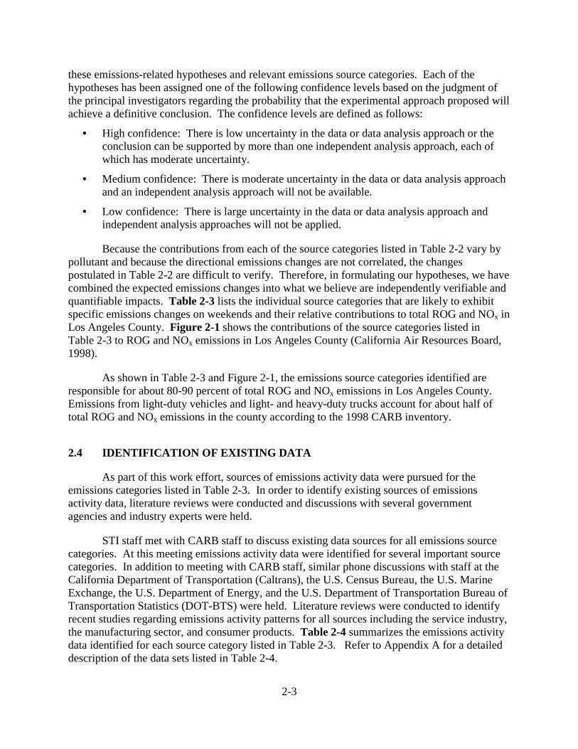
Because the contributions from each of the source categories listed in Table 2-2 vary bypollutant and because the directional emissions changes are not correlated, the changespostulated in Table 2-2 are difficult to verify. Therefore, in formulating our hypotheses, we havecombined the expected emissions changes into what we believe are independently verifiable andquantifiable impacts. Table 2-3 lists the individual source categories that are likely to exhibitspecific emissions changes on weekends and their relative contributions to total ROG and NOx inLos Angeles County. Figure 2-1 shows the contributions of the source categories listed inTable 2-3 to ROG and NOx emissions in Los Angeles County (California Air Resources Board,1998).

As shown in Table 2-3 and Figure 2-1, the emissions source categories identified areresponsible for about 80-90 percent of total ROG and NOx emissions in Los Angeles County.Emissions from light-duty vehicles and light- and heavy-duty trucks account for about half oftotal ROG and NOx emissions in the county according to the 1998 CARB inventory.

2.4 IDENTIFICATION OF EXISTING DATA

As part of this work effort, sources of emissions activity data were pursued for theemissions categories listed in Table 2-3. In order to identify existing sources of emissionsactivity data, literature reviews were conducted and discussions with several governmentagencies and industry experts were held.

STI staff met with CARB staff to discuss existing data sources for all emissions sourcecategories. At this meeting emissions activity data were identified for several important sourcecategories. In addition to meeting with CARB staff, similar phone discussions with staff at theCalifornia Department of Transportation (Caltrans), the U.S. Census Bureau, the U.S. MarineExchange, the U.S. Department of Energy, and the U.S. Department of Transportation Bureau ofTransportation Statistics (DOT-BTS) were held. Literature reviews were conducted to identifyrecent studies regarding emissions activity patterns for all sources including the service industry,the manufacturing sector, and consumer products. Table 2-4 summarizes the emissions activitydata identified for each source category listed in Table 2-3. Refer to Appendix A for a detaileddescription of the data sets listed in Table 2-4.

2-4

As shown in Table 2-4, there are multiple sources of activity data for most mobile sourcecategories. However, weekend activity data for industry and consumer product use is scarce.Discussions with CARB staff revealed that although temporal activity profiles are assigned to allindustrial, manufacturing, and consumer product emissions categories, these profiles do notreflect differences between weekday and weekend activity patterns. Furthermore, there has beenlittle, if any, work done to assess day-of-week activity patterns.

As part of Phase II, we will continue to gather and compile existing information and datathat will support weekend-weekday comparisons of emissions. Our efforts will be focused onidentifying and obtaining additional activity data for industrial, manufacturing, residential, andconsumer sources, since considerable data for on-road mobile sources have already beenidentified for analysis.

2.5 CHARACTERIZATION OF EMISSIONS ACTIVITY SURROUNDINGSELECTED AMBIENT MONITORING SITES IN THE SOCAB

As part of the field study to be conducted during the summer of 2000, DRI will collectambient measurements for use in Phase III to test hypothesized relationships between emissionssources and VOC/NOx ratios and ozone. In order to identify these relationships, emissionssources surrounding each ambient monitoring site were characterized in order to identify sourcesthat may impact ambient measurements. Unique sources of emissions within 5 km of each sitewere identified, including stadiums, parks, and recreation areas that may have different impactson ambient measurements on weekdays and weekends.

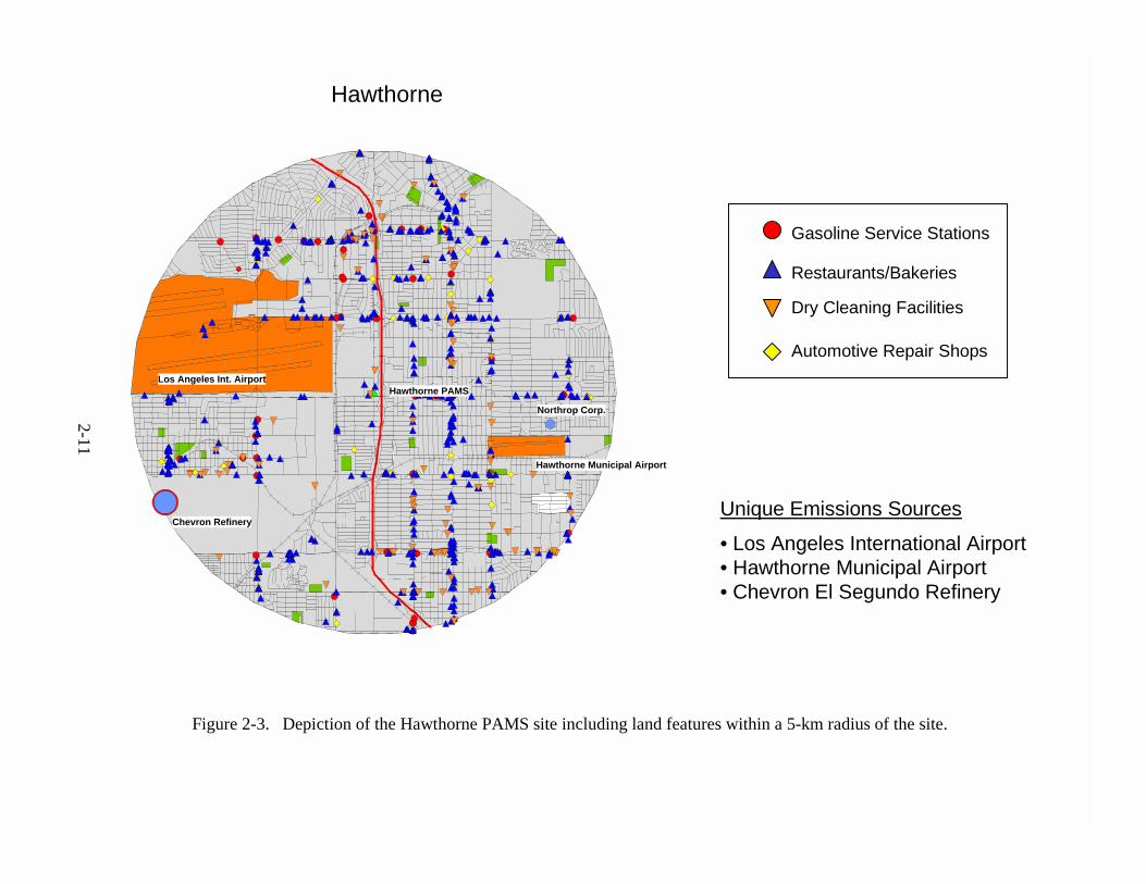
There are six ambient PAMS sites located throughout the SoCAB. These sites are listedin Table 2-5. In addition to the PAMS sites in the SoCAB, there is a monitoring site located inLos Angeles (Los Angeles North Main) that would be considered a Type 2 site under the PAMSclassification scheme. Figure 2-2 shows the locations of the six PAMS sites and the LosAngeles North Main long-term trend site. Figures 2-3 through 2-9 depict each of the ambientmonitoring sites and land features located within a 5-km radius of each site.

Because the SoCAB is dense with freeways and road networks, all of the sites are heavilyinfluenced by motor vehicle emissions. Emissions sources within 5 km of all of the monitoringsites (with the exception of Banning) consist of many service facilities (i.e., gas stations,restaurants, dry cleaners, and auto body shops). The following provides a summary of theunique emissions sources surrounding each of the ambient monitoring sites for which data maybe pursued further in Phase II. As part of the PAMS Data Analysis for Southern CaliforniaProject (Main et al., 1999) conducted in 1999, all of the ambient monitoring sites in the SoCABwere assessed in terms of how well the PAMS measurement systems represent the ambientSoCAB air. In addition to normal on-road vehicular traffic on surface streets and highwaysunique characteristics of the selected monitoring sites are discussed below.

• Hawthorne. Unique emissions sources near the Hawthorne site include Los AngelesInternational Airport, Hawthorne Municipal Airport, and the Chevron El SegundoRefinery. Based on historical analyses of ambient hydrocarbon data collected atHawthorne, VOC concentrations, composition, and ratios are consistent withHawthorne’s PAMS Type 1 designation (Main et al., 1999).

2-5

• Burbank. Unique emissions sources near the Burbank site include the Burbank-Glendale-Pasadena Airport and three major parks and recreation areas. Based on historicalanalyses of ambient hydrocarbon data collected at Burbank, it was determined thatnearby hydrocarbon sources may dominate many of the samples collected at Burbank(Main et al., 1999).

• Pico Rivera. Unique emissions sources near the Pico Rivera site include the WhittierNarrows Recreation Area and a bag printing company. Based on historical analyses ofambient hydrocarbon data collected at Pico Rivera, it was discovered that a nearby sourceof toluene appears in the daytime data (Main et al., 1999).

• Banning. Banning is located in the eastern region of the SoCAB in Riverside County.There appear to be no unique emissions sources near the monitoring site. Banning isdesignated as a PAMS Type 2 site (as listed in the Environmental Protection Agency’sAerometric Information Retrieval System [EPA AIRS]), however, the concentration,composition, and ratio data are more characteristic of a Type 4/1 site for the greater LosAngeles area (Main et al., 1999).

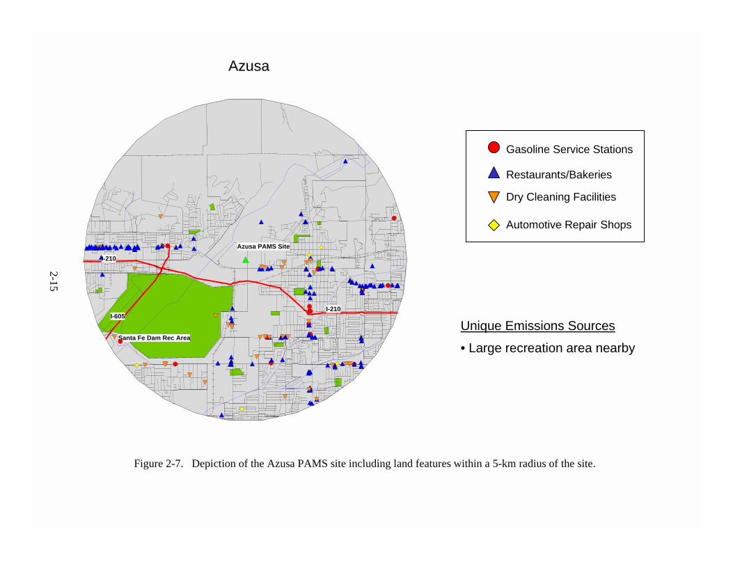
• Azusa. The Azusa monitoring site is located near the Santa Fe Dam Recreation Area andappears to be more suburban than the other sites. The VOC data show characteristics ofboth fresh emissions and aged, transported emissions (Main et al., 1999).

• Upland. There are three colleges and a small airport located within the 5-km radius ofthe Upland site. It appears to be a fairly urban site with many service facilities nearby.Based on historical analyses of ambient hydrocarbon data collected at Upland, VOCconcentrations, composition, and ratios are consistent with Upland’s PAMS Type 3designation (Main et al., 1999).

• Los Angeles North Main. The Los Angeles North Main long-term trend site is locatednear the intersection of two major freeways: the Pasadena and the Hollywood freeways.Dodger Stadium and Elysian Park are located slightly north of the site. VOC data areconsistent with CBD emissions.

2.6 DISCUSSION OF PHASE II DATA COMPILATION

The objectives of the Phase III data analyses will be (1) to quantify the weekend-weekdayvariations in anthropogenic emissions patterns that are most likely to impact air quality, and(2) to combine these results with air quality and meteorological data to test our hypotheses.Mobile sources, estimated to be the most important contributor of ozone precursor emissions inthe SoCAB, are known to follow pronounced weekday-weekend patterns of activity; thus, theywill receive a more in-depth focus in Phase II.

There are many measures of on-road travel activity and several ways to compare thembetween weekdays and weekends. A few examples are listed below.

• Vehicle miles traveled (VMT) • Vehicle Speeds • Fleet mix (trucks vs. cars)

2-6

• Cold/warm engine starts • Trips (frequency, length, and geographic pattern) • Trip chaining • Cars [sports utility vehicles (SUVs) versus commuter cars] • Diurnal patterns

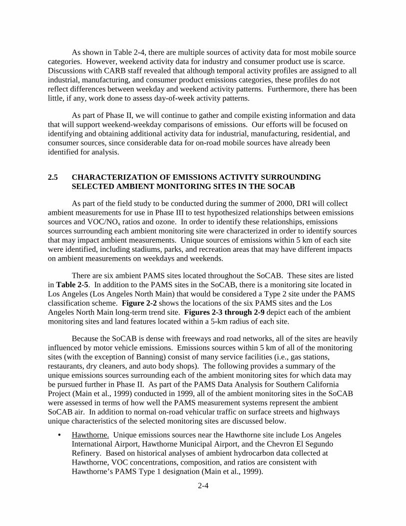
Figure 2-10, reproduced here from the Highway Capacity Manual, illustrates thetraditional view of weekend vs. weekday travel activity patterns. Urban freeway (UF) trafficbuilds gradually from Monday through Friday, drops off on Saturday, and drops even further onSunday. Rural (MR) and recreational (RA) routes have minimum traffic volumes mid-week,with pronounced peaks on Friday and Sunday. This result has been repeated for numerous urbancenters, especially for Los Angeles. In a 1993-1995 study of Los Angeles vehicles equippedwith data loggers, Magbuhat and Long (1996) showed that the frequency of cold starts followsthe same general pattern as the urban traffic volumes illustrated in Figure 2-10 (see Figure 2-11).Additionally, several EPA reports document weekend-weekday activity information. Two recentEPA publications (Glover and Brzezinski, 1998a,b), reflect the results of instrumented vehiclestudies in Spokane and Baltimore. Figures 2-12 through 2-14 illustrate Glover and Brzezinski’sconclusions that weekend urban travel levels are lower than weekday travel levels. Additionally,the data illustrate that most weekend travel tends to begin at a later hour of day than weekdaytravel and that it continues to be relatively uniform throughout the day (Glover and Brzezinski,1998a,b).

Traditionally, travel diaries have not collected weekend travel data so there are relativelyfew comparisons illustrating the differences between weekday and weekend travel activity.Several efforts are currently underway to better evaluate the relative importance of weekendversus weekday activity. For example, the Georgia Institute of Technology has gatheredcommercial vehicle data for Atlanta and plans to gather personal vehicle activity data during anupcoming survey (Guensler, 1999). In another example, the Texas Transportation Institute (TTI)has collected data for several counties in the Houston Metropolitan Statistical Area (MSA),where TTI counted and classified vehicles for Sunday, Monday-through-Thursday, Friday, andSaturday during the non-school year. TTI has used these data to distribute VMT by hour and byday-of-week into these four-day groups (Dresser, 1999). In addition, work is ongoing insouthern California to evaluate the relative importance of weekend vs. weekday travel in thisarea. Dr. Debbie Niemeier with the University of California at Davis recently completedanalyses for the CARB that will help further the knowledge base of weekend vs. weekday travelin southern California (Niemeier et al., 1999). The SCAQMD is also studying these sameweekend vs. weekday issues (Hsiao, 1999).

One illustration of the growing importance of weekend vs. weekday activity involvesdata from southern California. Several years ago, staff from the SCAQMD in Los Angeles usedCaltrans traffic count data to contrast average weekday vs. average weekend traffic counts for allvehicle types. They found that weekend travel counts were approximately 96 percent ofweekday travel counts and that weekend travel occurred more uniformly throughout the day, asopposed to the pronounced peak periods which are characteristic of weekday travel. Morerecently, SCAQMD staff have attempted to use truck traffic counts to better understand weekendvs. weekday heavy-duty vehicle activity. They have roughly estimated weekend truck trafficcounts to be approximately 40 percent of the truck traffic observed during an average weekday

2-7

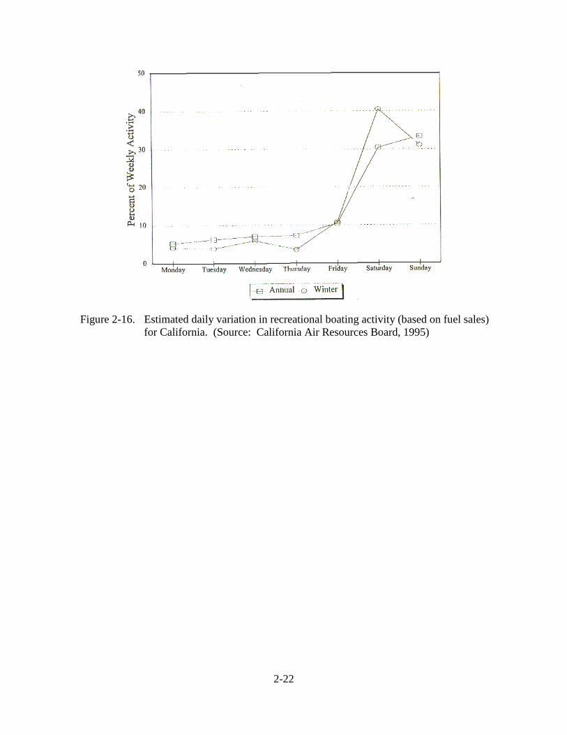
(Hsiao, 1999). Similar observations have been documented by the Transportation ResearchBoard (Figure 2-15). The opposite phenomenon is observed for recreational boating patterns inCalifornia. Weekend recreational boating activity levels are six to eight times higher thanweekday activity levels (Figure 2-16).

Historically, most detailed ozone photochemical modeling has focused on weekdayozone exceedance events. Furthermore, most emission control programs have focused onstationary sources and on reducing emissions associated with commuting. Thus, it should notcome as a surprise that very little attention has been paid to the development of accurateweekend emissions. Some adjustment factors to scale weekday emissions for use in modelingweekend days have been developed by CARB and the EPA. However, these scaling factors arebased on limited data and result in weekend emissions that are slightly lower than weekdayemission totals and very slightly alter the diurnal emissions pattern.

As uncertain as weekend emissions appear, weekday emission estimates are also underconsiderable doubt. A number of researchers have shown that published average daily weekdayemissions may underestimate real-world hydrocarbon emissions by as much as a factor of two ormore (see, for example, Fujita et al., 1992, 1994; Korc et al., 1993, 1995; Gertler and Pierson,1996; and Haste et al., 1998a,b). These results are fairly consistent throughout the country andthroughout California. A top-down approach, wherein ambient measurements of air quality,either from existing air quality monitoring sites or from special monitors placed in roadwaytunnels, has been used in many studies. Comparisons between the measured concentrations andpredicted emissions show that the inventory for weekdays consistently underpredictshydrocarbons, mostly, but not exclusively, from on-road mobile sources.

Because of the underestimates in the published weekday emission inventories, one cannotreliably use published estimates of differences in weekday and weekend emissions. Systematicdiscrepancies between observed and predicted emissions on weekdays may not apply to weekendemissions. Thus, in this study, independent and verifiable differences in emissions must beidentified.

Detailed analyses of the differences between predicted emissions and observedhydrocarbon data show that the standard speciated emission inventories are not representative ofambient air quality data. This discrepancy can in part be attributed to outdated orunrepresentative profiles used to speciate total hydrocarbon emissions into individual chemicalcompounds measured in the ambient air. Particularly noteworthy is the lack of speciationprofiles for recently introduced reformulated gasoline and reformulated solvents, inks, andsurface coatings. The use of unrepresentative speciation profiles complicates the identificationof differences between weekday and weekend day emissions from source types contributingsignificant hydrocarbon emissions. In Phase III, we plan to use the most recent source speciationprofiles available to improve the success of this study.

Specific emissions changes on weekends may include the following:

• Increased refueling of gasoline-fueled vehicles (including Friday) • Decreased number of trips of gasoline-fueled vehicles

2-8

• Increased home-related activity (e.g., lawn and garden equipment, surface coatings,paints, backyard barbecues, etc.)

• Decreased commercial-related activity (e.g., lawn and garden equipment, surfacecoatings, paints, etc.)

• Increased recreational activities (boating and other off-road mobile sources) • Decreased industrial activity • Decreased diesel (truck, bus, and train) activity • Decreased commuter activity (shifts time and location of on-road mobile source

emissions) • Increased use of utility vehicles for personal use • Decreased trip chaining

Because each of the activities listed emits different hydrocarbons, it should be possible totrace these types of changes with ambient data as well as estimate the changes throughinformation gathered using limited telephone surveys.

During Phase II of this study, we will compile data that can be used to assess possibleweekend effects. We will compile data for the year 2000 as well as historical data for 1997. Tothe extent that data can be obtained, we will produce graphics and statistics such as those shownin the examples above for emissions-related activity differences between weekdays andweekends. Our priorities in compiling emissions-related activity data are collecting(1) monitoring site-specific data, (2) SoCAB-specific data, (3) California-specific data, and(4) typical data from locations throughout the country where available.

Light Duty P as s enger Vehic les

31%

Co mmerc ia l/Indus tria l Mo bile Equipment

4%

Light Duty Trucks11%

Ships , Co mmercia l Bo a ts , Aircraft, Tra ins

2%

Mfg./Indus t.9%

Co atings and So lvents (Inc luding Architec tura l

Co atings )13%

Co ns umer P ro duc ts9%

P etro leum Marketing4%

Recreatio nal Vehic les3%

All Othe r Catego rie s14%

Ligh t Du ty P a sse nge r Ve h ic le s

15 %

Comme rc ia l/Ind us tria l Mob ile E qu ipme n t

13%

Ligh t Du ty Truc ks9%

He a vy Du ty Die se l Truc ks

6%

S h ips , Comme rc ia l Boa ts , Airc ra ft , Tra in s

11%

Mfg ./In dus t .3%

Re side n tia l Fue l Co mbustion

3%

P e tro le um Re fin ing (Combustion )

3%

Ligh t He a vy Du ty G a so line Truc ks

21%

All O th e r Ca te go rie s16%

Figure 2-1. Emissions source category contributions to total (a) ROG and (b) NOx inLos Angeles County. Mobile source emissions estimates are based onMVEI7G model. (California Air Resources Board, 1998)

Total ROG = 689 tons/day

Total NOx = 687 tons/day

2-9

a.

b.

Figure 2-2. Locations of selected PAMS and PAMS-like ambient monitoring sites in the South Coast Air Basin. Grey regions represent urban boundaries.

Hawthorne

LA N. Main

Burbank

AzusaUpland

Pico Rivera

Banning

Los Angeles Co.

Orange Co.

San Bernardino Co.

Riverside Co.

2-10

Gasoline Service Stations

Restaurants/Bakeries

Dry Cleaning Facilities

Automotive Repair Shops

Unique Emissions Sources

• Los Angeles International Airport• Hawthorne Municipal Airport• Chevron El Segundo Refinery

Figure 2-3. Depiction of the Hawthorne PAMS site including land features within a 5-km radius of the site.

Hawthorne

2-11

Los Angeles Int. Airport

Hawthorne Municipal Airport

Chevron Refinery

Northrop Corp.

Hawthorne PAMS






• Airport• Several Parks and Recreation Areas

Figure 2-4. Depiction of the Burbank PAMS site including land features within a 5-km radius of the site.

Burbank

Burbank-Glendale-Pasadena Airport

Burbank PAMS

Griffith Park

Stough Park

Wildwood Canyon Park

Brand Park

2-12






• Whittier Rec. Area• Printing company

Figure 2-5. Depiction of the Pico Rivera PAMS site including land features within a 5-km radius of the site.

Pico Rivera

Pico Rivera PAMS

Retail Center

Cmc Printed Bag Inc.

Whittier Narrows Rec. Area

So. Cal Gas Co.

2-13





Figure 2-6. Depiction of the Banning PAMS site including land features within a 5-km radius of the site.

Banning

Banning PAMS

I-10

I-10

2-14





Figure 2-7. Depiction of the Azusa PAMS site including land features within a 5-km radius of the site.

Azusa

I-605

I-210

Santa Fe Dam Rec Area

Azusa PAMS Site

I-210


• Large recreation area nearby

2-15





Figure 2-8. Depiction of the Upland PAMS site including land features within a 5-km radius of the site.

Upland


• Airport• Nearby colleges

Upland PAMS

Cable Land Co. Airport

Pomona College

Rancho Santa Ana Garden

I-10

I-10

Red Hill CC

Avery Fasson-Mpd

Upland Hills GC

2-16

Figure 2-9. Depiction of the Los Angeles North Main long-term monitoring site including land features within a 5-km radius of the site.

Los Angeles North Main


• Dodger Stadium• Elysian Park

Harbo

r Fwy.

Pasa

dena

Fwy.

Hollywood Fwy.

Echo Park

Elysian Park

Dodger Stadium

L.A. North Main Site




Traffic Count Data Collection


2-17

2-18

Figure 2-10. Examples of daily traffic variation by type of route. Legend: MR curverepresents main rural route I-35, Southern Minnesota, AADT 10,823,four lanes, 1980; RA curve represents recreational access route MN 169,North-Central Lake Region, AADT 3,863, two lanes, 1981; UF curverepresents urban freeway, four freeways in Minneapolis-St. Paul,AADTs 75,000-130,000, six to eight lanes, 1982. (Source: TransportationResearch Board, 1994)

2-19

Figure 2-11. Frequency of cold engine starts observed from 1993-1995 during a study ofinstrumented vehicles in Los Angeles (Magbuhat and Long, 1996).

0123456789

Weekday Weekend

Num

ber o

f trip

s pe

r day

CarsTrucks

Figure 2-12. Average weekend and weekday trip frequencies (Glover and Brzezinski, 1998a).

2-20

0

2

4

6

8

10

12

5 7 9 11 13 15 17 19

Hour (local time)

Perc

ent o

f Trip

s by

Hou

r

Weekday Weekend

Figure 2-13. Diurnal weekend and weekday distributions of trip frequencies, expressed as apercent of total weekend or weekday trips (Glover and Brzezinski, 1998a).

0

2

4

6

8

10

12

5 7 9 11 13 15 17 19

Hour (local time)

Perc

ent o

f VM

T by

Hou

r

Weekday Weekend

Figure 2-14. Diurnal weekend and weekday distributions of vehicle miles traveled expressed asa percent of total weekend or weekday VMT (Glover and Brzezinski, 1998a).

2-21

Figure 2-15. Daily variation in traffic by vehicle type. (Source: TransportationResearch Board, 1994)

2-22

Figure 2-16. Estimated daily variation in recreational boating activity (based on fuel sales)for California. (Source: California Air Resources Board, 1995)

2-23

Table 2-1. 1996 average daily emissions in the SoCAB (California Air Resources Board, 1998).

Emissions SourceROG

(tons/day)NOx

(tons/day)CO

(tons/day)Total – All Sources 1,100 1,100 6,100Stationary Sources 300 130 60Area-wide Sources 210 34 430On-Road Mobile Sources

Gasoline VehiclesDiesel Vehicles

50047822

700503197

4,2004,077

123Other Mobile Sources

Industrial VehiclesRecreational VehiclesNon-road (Trains & planes etc.)

99393822

250160

486

1,200870223107

Table 2-2. Summary of emissions changes hypothesized for weekdays versus weekend daysand relevant source categories.

Emissions Source Spatial Pattern Diurnal PatternDaily TotalEmissions

ConfidenceLevel

All Sources Spread out Spread out Lower MediumStationary Sources Lower in CBDa Spread out Mixed HighArea-wide Sources Higher in suburbs Higher in afternoon Higher MediumOn-Road Mobile Gasoline Vehicles Diesel Vehicles

Spread outHigher in suburbsLower in CBD

Spread outLower in a.m.Spread out

LowerLowerLower

High

Other Mobile Industrial Recreational Non-road (trains, airplanes, etc.)

Spread outLower in CBDHigher in suburbsLower in CBD

Spread outSpread outHigher in afternoonSpread out

MixedLowerHigherLower

Medium

a CBD is the central business district, i.e., downtown Los Angeles and the surrounding area of highest weekday emissionsand commerce.

2-24

Table 2-3. Emissions source categories hypothesized to exhibit changes in emissions betweenweekdays and weekends in Los Angeles County and their contributions to totalNOx and ROG emissions.

Emissions SourceCategory

Percent ofTotal ROGEmissions

Percent ofTotal NOxEmissions Emissions Change on Weekend

Light Heavy-DutyGasoline Trucks

<1% 20% • Decreased truck activity (delivery trucksetc.)

• Shifts in time and location of on-roadmobile source emissions

• Decreased number of trips of gasoline-fueled vehicles

Light-DutyPassenger Vehicles

30% 15% • Decreased commuter activity (shifts intime and location of on-road mobile sourceemissions)

• Increased refueling of gasoline vehicles(including Friday evening)


CommercialIndustrial MobileEquipment

4% 13% • Decreased industrial activity

Light-Duty Trucks 11% 9% • Decreased truck activity (delivery trucksetc.)


Heavy-Duty DieselTrucks

<1% 6% • Decreased diesel truck activity

Ships, CommercialBoats, Aircraft,Trains

2% 11% • Differences in diurnal activity patterns

ManufacturingCombustionDegreasingIndustrial

9% 3% • Decreased industrial activity

Coatings andSolvents (IncludingArchitecturalCoatings)

13% N/A • Decreased industrial activity• Increased consumer/residential activity

Consumer Products 9% N/A • Increased residential activityPetroleum Marketing 4% <1% • Differences in diurnal activity patternsRecreationalVehicles

3% <1% • Increased recreational activity

Source of Data: California Air Resources Board Emission Inventory for Los Angeles County, 1998.

2-25

Table 2-4. Summary of emissions-related activity data identified in Phase I, Task 1.

Emissions SourceCategory Type(s) of Activity Data Identified

Reference (seeAppendix A)

Light-, Medium-, andHeavy-Duty Trucks

• Caltrans WIM data for freeways• Vehicle counts on surface streets• Truck population, activity and usage

patterns report• Heavy-duty diesel truck activity data

collected by Battelle• A&WMA paper – fuel based emission

inventory for heavy-duty trucks• Off-road heavy-duty diesel vehicle activity

ABK

C

D

ELight Duty PassengerVehicles

• Caltrans WIM data for freeways• Vehicle counts on surface streets• Driving behavior characteristics• Traffic counts collected during SCOS97 on

freeways

ABF

L

Commercial/IndustrialMobile Equipment

• Nothing identified

Ships, CommercialBoats, Aircraft, Trains

• Marine activity data for Los Angeles andLong Beach harbors

• Report - California locomotive activity data• Airport activity data for LAX

J

IH

Manufacturing/Industrial • Nothing identifiedCoatings and Solvents(Including ArchitecturalCoatings)

• Activity profiles for auto-body refinishing,industrial/commercial adhesives andsealants, and metal products coating

• Nothing identified for architectural coating

E

Consumer Products • Nothing identifiedPetroleum Marketing • Internal CARB DocumentRecreational Vehicles • Activity profiles for recreational boating G

2-26

Table 2-5. PAMS sites in the South Coast Air Basin.

Site Type of SiteHawthorne Type 1Burbank Type 1/2Pico Rivera Type 2Banning Type 2Azusa Type 3Upland Type 4/1

Type 1 – Upwind background.Type 2 – Maximum precursor emissions, typically

located immediately downwind of CBD.Type 3 – Maximum ozone concentration.Type 4 – Extreme downwind transported ozone area.

3-1

3. UPPER-AIR METEOROLOGICAL AND AIR QUALITY ANALYSES

This section discusses meteorological and air quality analyses designed to improve thesummer of 2000 field study and future analyses.

3.1 OVERVIEW

The SoCAB has complex meteorology and air quality processes that result in largeday-to-day variations in ozone concentrations. A large portion of the variations in ozoneconcentrations are attributable to day-to-day variations in meteorology and not to the day-to-day(or weekday to weekend) variations in emissions. Therefore, in the absence of a large data set ofweekend and weekday ozone episodes, one must account for the effects of meteorology inanalyses that compare weekend and weekday episodes. Even with a modest size data set fromwhich to perform a statistical comparison, it is not likely that the weekend or weekday episodesare, on average, meteorologically similar enough to ignore the effects of meteorology.Furthermore, it is important to perform case study analyses along with any statistical analysisand meteorology must be taken into account in case study analyses.

Of the different parameters that represent meteorology, two that have a strong day-to-dayinfluence on ozone concentrations are winds and mixing heights. There are two ways that thesemeteorological characteristics might help us understand the variations in ozone concentrationsbetween weekend and weekdays. First, if we find selected weekend and weekday episode dayswith very similar meteorology and initial conditions, then we can compare and attributedifferences in the ozone concentrations to air quality processes and emissions and not tometeorological processes. Second, because it is not likely that there are many days to comparewith very similar meteorology, we will need to directionally quantify how mixing heights andwinds might influence ozone concentrations. Then, using directional influence information, wecan use a modest size data set from which to perform a statistical comparison that takes intoaccount meteorology.

To complete the described analyses, we must first be sure that we accurately represent themeteorology and, second, we must understand how the meteorology influences ozoneconcentrations. Furthermore, besides meteorology and emissions, aloft ozone also has someinfluence on surface ozone concentrations. Therefore, we need to understand the importance ofthe influence of aloft ozone and decide if it needs to be taken into account in the comparisoneffort. With these issues in mind, we set out to answer the following questions:

• What is the regional representativeness of the temporal and spatial variations in wind andmixing heights that can be obtained from the two Photochemical Assessment MonitoringStations (PAMS) radar wind profilers (RWPs) at Los Angeles International Airport(LAX) and Ontario (ONT) alone? (Sections 3.2 and 3.3)

• Does the 1997 Southern California Ozone Study (SCOS97) field study have bothweekend and weekday Intensive Operating Period (IOP) days that can be compared withone another? (Section 3.4)

3-2

• Is the meteorology on these IOP days similar enough to do a fair comparison of the airquality and emissions? (Section 3.4)

• How similar are the SCOS-97 episode days to Southern California Air Quality Study(SCAQS) 1987 episode days, based on the characteristics of the aloft ozone layers?(Section 3.5)

• What is the influence of the mixing heights and wind patterns on ozone concentration?(Section 3.5)

The results of analyses performed to address these questions are discussed in thefollowing sections.

3.2 REPRESENTATIVENESS OF MIXING HEIGHTS

This section evaluates the regional representativeness of the temporal and spatialvariations in mixing heights that can be obtained from the two PAMS profilers at LAX and ONTalone. Evaluation of the representativeness helps us determine whether the 2000 field study forPhase II of this project will require any additional radar profilers to accurately represent themixing heights at selected monitoring sites in order to understand the differences betweenweekend and weekday ozone concentrations.

Conceptually, we believe that information about winds and mixing heights areparticularly important in the middle and eastern part of the SoCAB (i.e., El Monte, Ontario, andRiverside) for understanding the weekend effect. It is in these areas where mixing heights andwinds can be either marine layer dominated or convective boundary layer dominated; and thetiming, evolution, and interaction of these phenomena can have a large impact on ozoneconcentrations.

In summary, we found that LAX and ONT do not spatially represent the temporal andspatial variations in mixing heights at two important areas in the SoCAB. On most episode days,neither LAX nor ONT represent the mixing heights in the middle of the basin (i.e., EMT) or inthe east basin (i.e., Riverside and Norton). Based on these results, we recommend that a radarwind profiler and radio acoustic sounding system (RASS) be operated in the vicinity of EMT andin the vicinity of Riverside (RSD) or Norton (NTN) during the 2000 field study. These twoprofilers, in addition to the LAX and ONT profilers, should produce the necessary mixing heightdata to represent areas throughout the basin, and, thus, allow us more complete data for anevaluation of the weekend effect.

To derive the representativeness conclusions, we performed a variety of data analysesusing products from radar wind profiler and RASS data collected at 16 sites that operatedthroughout Southern California during the SCOS97 field study (see Figure 3-1). In particular,we used CALMET wind fields, site observation of winds, and hourly mixing heights. TheCALMET wind fields and hourly mixing heights were produced as part of a work effort that weperformed for the South Coast Air Quality Management District (SCAQMD) (MacDonald et al.,2000 a,b) and were available for three high-ozone episodes (August 3-7, 1997; September 3-6,1997; and September 26-29, 1997).

3-3

3.2.1 Surface-Based Mixing Heights

In studies in several locations across the country (such as the northeastern United Statesand Houston and El Paso, Texas), the hourly diurnal profile of rising mixing heights in themorning and the peak mixing heights had a significant influence on maximum ozoneconcentrations (Dye et al., 1994, 1998; Lindsey et al., 1994; Roberts et al., 1997, MacDonald etal., 1998). Only since the installation of the two PAMS RWPs with RASS at LAX and ONT andduring SCOS97 have hourly mixing heights been available for the SoCAB.

In this work, the mixing height defines the top of the surface-based mixed layer. Thesurface-based mixed layer is the portion of the planetary boundary layer (PBL) above the surfacethrough which vigorous vertical mixing of heat, moisture, momentum, and pollutants occurs(Holtzworth, 1972). During the daytime at inland sites, the mixing height is defined as thealtitude of a stable layer, or an inversion capping a well-mixed convective boundary layer (CBL).At night, identification of the top of the mixed layer is more complicated because often severalstratified layers exist below the base of a well-defined inversion and vertical mixing is confinedto the lowest tens or hundreds of meters. At coastal sites, the surfaced-based mixing height isdefined as the top of the marine boundary layer.

The RWP measures, as a function of height, wind speed and direction and the radarsignal-to-noise ratio, which can be used to estimate mixing height. The RASS portion of thesystem measures temperature as a function of altitude; the temperature data can also be used toestimate mixing heights. The mixing height data can be used to help understand the processesthat might influence weekend/weekday differences in ozone concentrations and evaluate themeteorological similarity of weekend and weekday days.

As discussed in MacDonald et al. (2000b), RASS virtual temperature data coupled withsurface temperature data were used to estimate hourly surface-based mixing heights when themixing height was below the maximum height of the RASS profile [at about 1000 m aboveground level (agl)]. This typically meant that RASS data were used to estimate the mixingheights at night and during the early morning hours at all sites. Furthermore, RASS data wereoften used to estimate the mixing heights all day at coastal sites where mixing heights arestrongly influenced by the marine boundary layer and where the marine boundary layer rarelyexceeded the maximum height of the RASS virtual temperature profile. At inland sites, whenthe convective boundary layer exceeded about 1000 m agl, the refractive index structureparameter (Cn

2) and vertical velocity data were used to estimate the mixing heights. Cn2 indicates

the fluctuations of the index of refraction, which are primarily due to fluctuations in the watercontent of air. Fluctuations in water content are strongest near boundaries, such as at the top of theCBL. Both theoretical and empirical studies have shown that Cn

2 peaks at the inversion located atthe top of the CBL due to warm, dry, aloft air entraining into cooler, moister air below theinversion (for example, Wyngaard and LeMone, 1980). Generally, Cn

2 estimated from RWPs willnot resolve low-level inversions below 200 to 300 m agl.

3-4

3.2.2 Mixing Height Characteristics

There are several characteristics of mixing heights that have been shown to be importantto peak ozone concentrations and may be important in understanding differences betweenweekend and weekday air quality, and there are others that we hypothesize may be important.The following mixing height characteristics were considered in our evaluation ofrepresentativeness.

Peak daytime mixing height

Perhaps the most important and the most commonly assessed characteristic of mixingheight is the peak daytime mixing height. The peak mixing height often occurs in the earlyafternoon around the time of the daily peak ozone concentration. The peak mixing heightcontrols the maximum vertical dilution of ozone and its precursors. If the peak mixing height ishigh, then the vertical dilution of surface ozone at this time is large and ozone concentrationswill probably be lower compared to when the peak mixing height is low and the vertical dilutionof ozone is small. Obviously, as the mixing height grows during the day, it entrains aloft air.The chemical composition of this aloft air can affect the surface ozone concentration. If the aloftair is clean, then rising mixing heights will dilute surface ozone and precursor concentrations. Ifaloft air is polluted, surface concentrations may not show a significant change.

Mixing growth rate

Another characteristic of the mixing height that has received recent attention is themixing growth rate (MGR) (Dye et al., 1994, 1998; Lindsey et al., 1994; Roberts et al., 1997;MacDonald et al., 1998). The MGR often characterizes the morning transition of the mixedlayer from the nocturnal boundary layer to the convective boundary layer prior to the peakmixing height. In coastal areas, the MGR may represent the evolution of the marine boundarylayer. For this project the MGR has been chosen to be the rate of growth from 0700 to1200 PST. During this time, important ozone forming chemistry takes place, and the verticaldilution of ozone and ozone precursors may result in peak ozone concentrations that aredifferent, even if the peak mixing heights are similar. The mixing growth rate may be animportant key to understanding how weekend and weekday emission differences can result indifferent ozone concentrations. If the weekend emissions are more reactive compared toweekday emissions, then a day with a fast mixing growth rate may result in different ozoneconcentrations on a weekend compared to a weekday.

Mid-morning average mixing height

A mixing height characteristic similar to the MGR is the mid-morning average mixingheight. For this project, the mid-morning average mixing height was chosen to be the averagemixing height from 0900 to 1100 PST. This parameter may be an important characterization ofmixing height for evaluating the weekend effect because during the mid-morning importantozone forming chemistry occurs. Differences in the vertical dilution of ozone and ozoneprecursors in the mid-morning may result in peak ozone concentrations that are different, even ifthe peak mixing heights are similar.

3-5

Time of peak mixing

The time of peak mixing height may also be another important characterization of mixingheight for evaluating the weekend effect. If the convective boundary layer grows quickly andpeaks early in the day, then the maximum vertical dilution of ozone precursors and ozone alsooccurs early. Again, if weekend emissions have a different ozone production rate, then aweekend day with an early peak in mixing height may produce different ozone concentrationscompared to a weekday with similar meteorology.

Early morning mixing height

The early morning mixing height gives information on the state of the system at the startof the day, when ozone-producing chemistry begins. If the early morning mixing height (0200 to0600 PST average mixing height for this project) is high, then the overnight emissions werediluted into a larger volume than if the mixing height is low. The resulting differences inchemical concentrations within the mixed layer at the start of the day could have an influence onthe peak ozone concentration. Therefore, early morning mixing heights may need to beaccurately represented to understand the weekend effect.

3.2.3 Method for Evaluating Mixing Representativeness

Using the hourly mixing heights from the 16 RWP/RASS stations (see Table 3-1) withinthe SoCAB, we performed a variety of objective and subjective data analyses to evaluate therepresentativeness of the LAX and ONT hourly mixing heights. The coastal sites include PortHueneme (PHE), Los Alamitos (LAS), LAX, Carlsbad (CBD), San Clemente Island (SCE),Santa Catalina Island (SCL), and Tustin (TTN); mid-basin sites include Central Los Angeles(USC), El Monte (EMT), Van Nuys (VNS), Simi Valley (SMI), and Valley Center (VLC); andeast-basin sites include ONT, NTN, RSD, and Temecula (TCL). Figure 3-1 shows the locationsof all sites, and Table 3-1 lists the site names, three-letter identifier, position, and elevationinformation. We performed the following:

• For each site for each of the 13 episode days, we calculated the peak daytime mixingheight, the 0700 to 1200 PST mixing growth rate, the 0900 to 1200 PST mid-morningaverage mixing height, the time of peak mixing, and the 0200 to 0600 PST early morningmixing height. Using these data, we performed cluster analyses to determine how thesites group by each of these variables. We also performed cluster analyses on threesubsets of days including a westerly sea breeze (day type 1), a southerly sea breeze (daytype 2), and an offshore flow (day type 3).

• We calculated how often the hourly mixing heights from each site are within the greaterof 200 m or 25 percent of the hourly mixing heights at LAX or ONT. These criteria werechosen because past studies comparing profiler- and RASS-derived mixing heights torawinsonde-, aircraft pollutant-, and turbulence-derived mixing heights had root meansquare differences of 200 m. Because mixing heights have different nighttime anddaytime characteristics, we divided the data by daytime only, nighttime only, and all timeand performed the calculations.

3-6

• We calculated the correlation coefficients for the hourly mixing height data betweenLAX and all other sites and between ONT and all other sites. We also created a datasetof “binned” mixing heights to remove the noise associated with uncertainties in themixing height estimates. These binned mixing heights were created by setting the hourlymixing heights at a candidate site equal to the mixing heights at LAX or ONT if thehourly mixing heights at the candidate site were within the greater of 200 m or 25 percentof the hourly mixing heights at LAX or ONT. Again, we divided the frequency ofoccurrence by daytime only, nighttime only, and all time.

• We created scatter plots of hourly mixing heights at LAX and other coastal sites andONT and mid- and east-basin sites.

• We plotted and subjectively analyzed time-series plots of mixing heights at the16 RWP/RASS stations.

• We plotted and subjectively analyzed hourly spatial contour plots of mixing heights usingdata from stations throughout the SoCAB and surrounding areas.

• We plotted the east-basin, mid-basin, and coastal sites’ daily average peak afternoonmixing heights. We then compared the daily average peak mixing height of each regionto the daily peak mixing height at LAX, EMT, ONT, and RSD.

3.2.4 Mixing Results and Conclusions

Neither LAX nor ONT spatially represent the temporal and spatial variations of mixingheights at two important areas in the SoCAB. On most episode days, neither LAX nor ONTrepresent the mixing heights in the middle of the basin, including the mixing heights at USC,EMT, VNS, SMI, and VLC or in the far east basin including NTN, RSD, and TCL.Furthermore, the analyses suggest that EMT and RSD are representative of the mid-basin andeast basin, respectively. Examples of the analyses from which these conclusion were derived arepresented below.

Subjective review

Time-series plots and spatial contour plots of hourly mixing heights indicate that themixing heights derived from the radar profiler and RASS data are conceptually reasonable.Mixing heights at coastal sites show little diurnal variability indicating a marine layer-dominatedboundary layer. Whereas, the far inland sites show a strong diurnal cycle from the nocturnalboundary layer to the convective boundary layer, with little apparent marine influence. Finally,the mid-basin sites have more diurnal variability than the coastal sites, but the height of theconvective boundary layer growth is only half as much as the inland sites. The limited CBLgrowth at these sites is likely due to cool marine air suppressing the convective mixing.

In terms of representativeness, the time-series plots indicate that mixing heights at LAXare representative of the mixing heights at coastal sites and not the mid-basin sites, as expected.For example, the time-series plots of hourly mixing heights on September 3-4, 1997, show thatmixing heights at LAX ranged from 250 m agl to only 600 m agl (Figure 3-2). Despite thehourly variability in mixing heights, the relatively steady mixing heights at LAX are similar and

3-7

representative of other coastal sites such as CBD, SCE, SCL, and PHE but are not representativeof mid-basin sites such as USC, EMT, VNS, and SMI.

ONT, which has a diurnal cycle from the nocturnal to convective boundary layer, withsome indications of a marine influence, has a diurnal pattern similar to those of the mid-basinand east-basin sites; however, the maximum mixing heights do not represent any site oftenenough to be representative. For example, on some days, such as September 26, 1997, ONT issomewhat representative of a mid-basin site such as EMT; whereas, on other days, such asAugust 4, 1997, ONT is not similar to EMT, but is similar to an inland site such as RSD.

The average coastal, mid-basin, and east-basin regions each have distinct daily peakmixing heights (Figure 3-3). Comparing the three regions daily average peak mixing heights toother sites further illustrates that LAX represents coastal sites, and ONT waivers betweenrepresenting a mid-basin site and east-basin sites. As shown in Figure 3-3, the peak mixingheights at coastal sites are about 500 m and show little day-to-day variability. The peak mixingheights at mid-basin sites are about 800 m during the August episode and about 1400 m duringthe September episodes. The peak mixing heights at east-basin sites have the greatest variability,ranging from about 900 m on August 7 to about 2900 m on September 3 and 4. Comparison ofthe daily peak mixing heights at LAX to the coastal and mid-basin average peak mixing heightsindicates that peak mixing heights at LAX are representative of the coastal average, but are notrepresentative of the mid-basin average (Figure 3-4). Comparison of the daily peak mixingheights at ONT to the mid-basin and east-basin averages indicates that peak mixing heights atONT are sometimes representative of the mid-basin average and sometimes representative of theeast-basin average (Figure 3-5). Comparison of the daily peak mixing heights at EMT to thedaily peak mixing heights in the mid-basin indicates that the peak mixing heights at EMT arerepresentative of the mid-basin average (Figure 3-6). Finally, comparison of the daily peakmixing heights at RSD to the daily peak mixing heights in the east basin indicates that the peakmixing heights at RSD are generally representative of the east-basin average (Figure 3-7).

Cluster analyses

Cluster analysis is a multivariate procedure for detecting natural groupings in data. Thisanalysis provides a graphical depiction of the relationships among data groupings, such as dailypeak mixing heights collected at different sites. To produce clusters, one must be able tocompute some measure of dissimilarity between objects and two methods are commonly used todo this: correlation measures and Euclidean measures. Correlation measures are not influencedby differences in scale between objects. This method measures the similarity in patterns acrossdata regardless of overall magnitude. Euclidean or City Block Distance measures aresignificantly affected by differences in scale but are useful for variables that share a commonscale such as in this project.

Depending upon the complexity of the data at a site, one to several clusters may beneeded to account for a majority of the variability in the data. One variable in a cluster could beconsidered a surrogate for the other variables in the cluster. In general, the larger the distancebetween variables, the less similar their variability.

3-8

Cluster analyses were performed using the peak daytime mixing height, the mixinggrowth rate, the mid-morning average mixing height, the time of peak mixing, and the earlymorning mixing height. To interpret Figure 3-8, consider a vertical line drawn at an arbitrarydistance of about 200. Dissecting the figure at 200 appears to be a logical break in the number ofclusters. We could just as easily select 300 in this example to reduce the number of clusters toconsider. In the figure, LAX daily peak mixing heights cluster with San Clemente Is., SantaCatalina Is., Port Hueneme, and Carlsbad, all coastal sites. In contrast, the peak daily mixingheights observed at the inland sites of Riverside, Norton, and Temecula do not cluster with therest of the data, indicating that the peak mixing height did not behave similarly. Other resultsshow that LAX grouped well with all coastal sites for all parameters except for the average earlymorning mixing height and the time of peak mixing. Whereas, ONT grouped poorly with allsites for all parameters. For example, as shown in Figure 3-8, for the peak mixing height cluster,LAX grouped well with SCE, SCL, PHE, and CBD [Euclidean (root mean square) distances lessthan 200 m], fair with TTN, LAS, VLC, USC, and EMT (Euclidean distances between 200 and250 m), and poor with the east-basin sites (Euclidean distances greater than 400 m). ONT, onthe other hand, did not group well with any site (Euclidean distances greater than 400 m for thisparameter).

For the most part, the cluster analyses by day type showed results similar to those of theall day’s cluster analyses, with a few exceptions. For all parameters, except the early morningmixing height and time of peak, there were better groupings among coastal sites on day types 2and 3 (southerly sea breeze and offshore days, respectively) compared to day type 1 (westerlysea breeze). Also, the peak mixing height at mid-basin sites grouped best on day type 2(Euclidean distances less than 200 m). Furthermore, the mid-basin site, EMT, grouped very wellwith LAX (Euclidean distances of 80 m) on day type 2.

Correlations, scatter plots, and frequency bins

The correlation coefficients (r) of hourly mixing heights and frequency of equal mixingheight are summarized in Table 3-2 for ONT and Table 3-3 for LAX. In these tables,correlation coefficients greater than 0.6 are bold and frequencies greater than 0.7 are bold formixing heights that are within the greater of 200 m or 25 percent of LAX or ONT. Scatter plotswere used in the analysis to allow for a more robust interpretation of the correlations.

LAX correlated poorly with all sites, day or night. Despite LAX’s poor correlation, themixing heights were within 200 m or 25 percent of the coastal sites at least 60 percent of the timeduring the day and even more often at night. The higher frequency of agreement at night makessense because there is much smaller spatial variation in mixing heights at night compared toduring the day. These analyses indicate that despite a poor correlation with other sites, themixing heights at LAX reasonably represent the mixing heights at coastal sites during the dayand at night.

Mixing heights at ONT correlated fair to good with mixing heights at mid-basin andeast-basin sites and poorly with coastal sites. The correlation coefficients between ONT andRSD, NTN, and Simi Valley were about 0.7 for all times. Despite the high correlation with thesesites, the frequency of the mixing heights being within the greater of 200 m or 25 percent wasonly around 50 percent during the day for the mid- and east-basin sites. At night, the frequencies

3-9

were much higher. The positive correlation during the day and the relatively poor frequencynumbers during the day mean that although the hourly mixing heights at ONT have similar dailycycles, the magnitudes of the cycles are not similar. Furthermore, as the scatter plot of hourlymixing heights between ONT and RSD shows (Figure 3-9), the good correlation between thesesites is driven by mixing heights below 1000 m. When mixing heights at RSD are 2000 to4000 m agl, the correlation between mixing heights at RSD and ONT sites is poor. Therefore,without a site near RSD, this important information that indicates high mixing heights east ofONT would be unavailable.

3.3 REPRESENTATIVENESS OF WINDS

As part of a work effort for the SCAQMD, MacDonald et al. (2000a) used wind datacollected by the 16 RWP during three high-ozone episodes in 1997 (August 3-7, September 3-6,and September 26-29) to develop three-dimensional CALMET diagnostic wind fields. Thelocations of the RWP are shown in Figure 3-1. Using the wind fields, we prepared hourlyCALMET wind-field plots for each episode day for three elevations:

• 40 m agl (level 1), 486 m agl (level 5), 1671 m agl (level 15) representing the surfacelayer;

• a layer within the midday mixed layer (e.g., 400 or 600 m agl); and

• a layer above the mid-basin midday mixed layer (e.g., 1000 to 2000 m agl).

Using these CALMET wind fields, in conjunction with the observed wind profiles at the16 sites shown in Table 3-1, we subjectively evaluated the regional representativeness of thetemporal and spatial variations in wind that can be obtained from profiler data collected at LAXand ONT alone.

In summary, we found that the aloft winds measured at LAX are reasonablyrepresentative of winds at other surrounding coastal sites including USC, LAS, TNN, and PHE,and are often not representative of winds at mid- or east-basin sites such as EMT, ONT, RSD,and NTN. Also, we found that the winds measured at ONT are reasonably representative ofwinds at other surrounding inland sites including RSD and NTN and are often not representativeof mid- basin or coastal sites such as EMT and LAX. Particular observations from the analysesare presented below.

During the three 1997 ozone episodes, a variety of meteorological conditions werecharacterized by the synoptic weather pattern, wind fields and mixing heights. A more detailedcomparison of these episodes is presented in Section 3-4. Of importance to our windrepresentative analysis are the varying wind-flow patterns. These patterns included strongwesterly sea breeze flow, moderate southerly sea breeze flow, light offshore easterly flow, andstrong offshore northerly flow. The representativeness of the aloft winds measured at LAX andONT depended on these flow types and flow strength. In general, the stronger the winds, themore representative the winds at LAX and ONT were of the winds in the rest of the SoCAB.Under light flow patterns, when local forcing tends to dominate the winds, LAX and ONT wereless representative of the winds in the rest of the SoCAB.

3-10

Because there are many surface monitors throughout the basin that represent the lowerlevel winds (i.e., 40 m agl) and because the winds at 1671 m agl are often above the boundarylayer, we focused our observations on the 486 m agl boundary-layer winds. Note that the figuresdescribed next are spatial plots of wind fields; the CALMET diagnostic wind fields are displayedas narrow arrows and the observations are displayed as bold fat arrows. Observations ofboundary-layer winds during the three SCOS97 episodes include the following:

• Under sea breeze conditions, there was no obvious timing delay in the start of onshoreflow during the day between the coastal sites and inland sites.

• Under strong sea breeze conditions, winds at LAX were representative of the winds in theentire basin including winds at RSD, ONT, and NTN. For example, Figure 3-10 showsthe wind field on September 4, 1997, at 1500 PST.

• Under moderate sea breeze conditions, winds at LAX were representative of the winds atUSC, TTN, LAS and often EMT. For example, Figure 3-11 shows the wind field onSeptember 26, 1997, at 0300 PST.

• Under light wind conditions, winds at LAX were often representative of the winds atUSC.

• Under westerly sea breeze conditions at LAX, the winds at TTN and LAS tended to bemore northwesterly.

• Under northerly or northeasterly flow in most of the mid- and east basin, winds at LAXwere generally not representative of the winds at most sites. For example, Figure 3-12shows the wind field on September 28, 1997, at 0900 PST.

• Under strong sea breeze flow, winds at ONT were representative of the winds at NTNand RSD; however, winds at RSD were, at times, northwesterly when winds at ONT andNTN were westerly. For example, Figure 3-13 shows the wind field on September 28,1997, at 1500 PST.

• Under offshore flow, wind direction at ONT was usually representative of wind directionat NTN and RSD, but the wind strength was sometimes lighter at ONT than at NTN andRSD. Winds at ONT were generally not representative of winds at EMT or coastal sitesunder the offshore flow pattern.

3.4 EVALUATION OF THE METEOROLOGY DURING THE SCOS97 OZONEEPISODES

The wealth of both air quality and meteorological data collected during the SCOS97 fieldstudy provides an excellent opportunity to add to our understanding of the weekend ozone effect.This section discusses the possibility of taking advantage of this episodic data set. To do so, wemust first determine if there were both weekend and weekday IOP days to compare. Second, ifthere were weekend and weekday IOP days, we must determine if the meteorology on these IOPdays is similar enough to do a fair comparison of the air quality and emissions.

In summary, there were two weekend episodes and three weekday episodes. In ouranalyses, we did not consider one of these weekday episodes (July 14) because we did not have

3-11

the necessary data readily available to complete our analyses. Of the four episodes, there werethree distinct synoptic meteorological patterns. Of the two episodes with similar synopticmeteorology, one was a weekend episode and the other was a weekday episode; therefore, theseepisodes are candidates for comparison of weekend and weekday air quality. Finally, becausethe meteorology of the ozone episodes is significantly different on some days, modeling of theweekend and weekday effect should be done using different meteorological patterns and not justone pattern.

To derive these conclusions, we analyzed the daily National Weather Service synopticweather charts, Eta Data Assimilation System (EDAS) archive, hourly mixing heightsthroughout the SoCAB, hourly CALMET wind fields for three elevations (40 m agl , 486 m agl,and 1671 m agl), and ozone data for each episode day. As mentioned previously, the hourlymixing heights and CALMET wind fields were developed as part of a work effort for theSCAQMD (MacDonald et al., 2000 a,b). As part of this project, we produced mixing heights fora fourth episode (August 22 and 23, 1997) at LAX, EMT, ONT, and RSD. These sites werechosen because Section 3-1 showed that mixing heights at these sites generally represent mixingheights throughout the basin.

During the SCOS97 field program there were four major IOP ozone episodes in theSoCAB including August 4-7 (Monday through Thursday), August 22-23 (Friday and Saturday),September 3-4 (Wednesday and Thursday), and September 26-27 (Saturday and Sunday). Thepeak 1-hr and 8-hr ozone concentrations for these episodes are shown in Table 3-4.

The August 4-7 episode was characterized by a strong upper-level ridge that built in fromthe east over Southern California (e.g., Figure 3-14). This resulted in weak offshore flow in theeast basin, light variable flow in west basin at night. and weak onshore flow during the day. Thestrong upper-level ridge also resulted in low mixing heights throughout the mid-basin (about750 m agl) and coastal sites (about 500 m agl) throughout the episode. The east basin also hadlow mixing heights on August 4 and 7, but had relatively high mixing heights in the middle ofthe episode. A summary of the peak mixing heights for all episodes can be found in Figure 3-3for the area averages and in Figure 3-15 for LAX, EMT, ONT, and RSD. Figure 3-15 wasadded because the area averages were unavailable for the August 22-23 episode.

The August 22-23 episode was characterized by a “battle” between an upper-level high-pressure system east of southern California and an upper-level trough of low pressure located offthe coast of northern California. With the trough offshore, and the ridge being unable to build inover southern California as it did during the August 4-7 episode, the sea breeze was strongerduring August 22-23 than during August 4-7. Also, the peak mixing heights at the mid-basin site(EMT) were slightly higher during August 22-23 than during August 4-7 but were similar at thecoast (LAX) and east basin (ONT and RSD) (e.g., Figure 3-15). These meteorologicaldifferences and their likely influence on ozone concentrations between the two August episodeswould probably overwhelm any signal from the differences in emissions between the weekdayepisode (August 4-7) and weekend episode (August 22-23). Therefore, these two Augustepisodes are not the best cases for comparison to understand the weekend effect.

Similar to the August 22-23 episode, the September 3-4 episode was characterized by a“battle” between an upper-level high-pressure system east of southern California and an upper-

3-12

level trough of low-pressure located off the coast of northern California. However, the troughwas not quite as dominant in the September 3-4 episode as during the August episode. Becauseof the weaker trough, the onshore flow during this episode was slightly weaker than the onshoreflow, and the offshore flow at night in the east basin was slightly stronger, compared to theAugust 22-23 episode. As shown in Figure 3-15, the peak mixing heights between theSeptember 3-4 episode and the August 22-23 episode were similar at LAX and EMT but lowerduring the August 22-23 episode at ONT and RSD. Despite the differences in onshore flowstrength and inland peak mixing heights, these two episodes probably have similar enoughmeteorology to be good candidates for a more detailed weekend and weekday analysis.

The September 27-29 episode was characterized by a strong surface high-pressure systemover the intermountain west (between the Sierra Nevada and Rocky Mountain ranges) with athermal trough along the coast. This pattern resulted in northerly flow at night that reached thecoast and weak onshore flow during the day, with the exception of offshore flow through SimiValley. Mixing heights were very similar to the September 3-4 episode, being low at the coast,moderate in the mid-basin, and relatively high in the east basin. Unlike September 3-4, however,there was strong offshore flow at the 850-mb level during September 27-29. This episode doesnot have meteorology similar enough to any of the other episodes to be a candidate for a moredetailed weekend and weekday analysis.

3.5 MIXING HEIGHTS, WINDS, AND ALOFT OZONE

Previous analyses of aloft ozone data from SCAQS have shown the presence of deeplayers (about 500 m) of high ozone concentrations over a wide portion of the SoCAB (e.g.,Roberts and Main, 1992). The aloft ozone can contribute to the surface ozone concentrationswhen mixed to the surface during the day. During SCOS97 a Lidar located at EMT collectedaloft ozone data from 90 m agl to about 2500 m agl during IOPs. Aloft wind and mixing heightdata were also collected at EMT. Using these data we evaluated the variability of thecharacteristics of these aloft ozone layers during ozone episodes and evaluated the similarity ofthe SCOS97 episode days to SCAQS 1987 episode days, based on the characteristics of the aloftozone layers and investigated the influence of the mixing heights and wind pattern on ozoneconcentrations.

We created time-height cross sections of ozone data (collected by the Lidar), mixingheights, and winds for four 1997 episode days. The episode days included August 4-5 (Mondayand Tuesday) and August 22-23 (Friday and Saturday). Originally, we wanted to use September3-4 instead of August 4-5 because, as discussed in the previous section, September 3-4 andAugust 22-23 had similar synoptic meteorology and were week days and weekend days,respectively. However, Lidar data were unavailable for September 3-4. We also createdtime-series plots of surface ozone and mixing heights at Upland/Ontario and Rubidoux/Riversidefor August 3-7, August 22-23, September 3-6, and September 26-29, 1997. For the evaluation ofthe similarity of the SCOS97 episode days to 1987 episode days, we reviewed aloft ozone datacollected at EMT on four 1987 episode days and compared these data to the aloft ozone datacollected on four 1997 episode days.

3-13

In summary, we found that the interaction among winds, mixing heights, and ozoneconcentrations is too complex to form any definitive conclusions (in this preliminary analysis)about their relationship and how their relationship might influence differences in ozoneconcentrations between weekdays and weekends. We recommend a more detailed investigationof mixing heights, winds, and ozone concentrations in Phase II. Also, we found that the morningaloft ozone concentrations at EMT for selected 1997 episodes were about half the aloft ozoneconcentrations observed during selected 1987 episodes. Although only a few days werecompared, the observation does suggest that contribution of aloft ozone to surface ozone may notbe as significant now as it was in 1987. Some details of our observations are presented below.

Although the relationship among the vertical structure of ozone, mixing heights, andwinds is too complex to form any definitive conclusions from these preliminary analyses,important observations were made. Several of these observations refer to Figures 3-16through 3-19. These figures show time-height cross sections of ozone data (collected by theLidar), mixing heights, and winds at EMT during 1997.

• Mixing heights are lower at EMT in the afternoon than during midday hours on all fourcase-study days. The lowering of the mixing heights appears to be associated with theintrusion of marine air undercutting the CBL.

• On August 4, despite the lowering of the inversion, boundary layer ozone concentrationsdecreased from about 100 ppb at 1400 PST to 60 ppb at 1600 PST (Figure 3-16). Thedecrease in ozone over this period is probably associated with clean marine air. A similarpattern was observed on August 5 (Figure 3-17). On the other hand, on August 23, ozoneconcentrations did not decrease at EMT when the afternoon mixing heights lowered, evenwith apparent marine intrusion (Figure 3-19).

• On August 5, there was a layer of high ozone concentrations between 500 and 1000 m aglduring 1400 to 1700 PST (Figure 3-17). The high ozone concentrations were above themixed layer at EMT. It is not clear where this pool of high ozone concentrations camefrom. The winds prior to this time were light easterly in the morning and strong westerlyduring the time of high ozone concentrations. Given the mixing height and the locationof the high ozone concentrations above the boundary layer, it appears that the high ozonedid not contribute to the surface ozone concentrations at EMT on this day.

• On August 4, there were no high concentrations of aloft ozone above the mixed layer.The winds above the mixed layer were from the northwest during the morning andafternoon (Figure 3-16).

• On August 23, there were three distinct layers of high ozone concentrations aloft(Figure 3-19). There was a thick layer of high ozone concentrations (130 to 150 ppb)between about 600 and 1000 m agl; this layer was above the mixed layer. Winds in thislayer were from the southeast until 1400 PST. At 1500 PST, when the plume appeared,the 1000 m agl wind was from the north. Below the mixed layer, there were two otherpools of high ozone concentrations: one at about 500 m agl and one at about 100 m agl.

• Time-series plots of surface ozone and mixing heights at Upland/Ontario andRubidoux/Riverside show no distinct relationship. For example (see Figure 3-20), onAugust 7, the peak mixing height at RSD was only 1000 m agl, and the peak surface

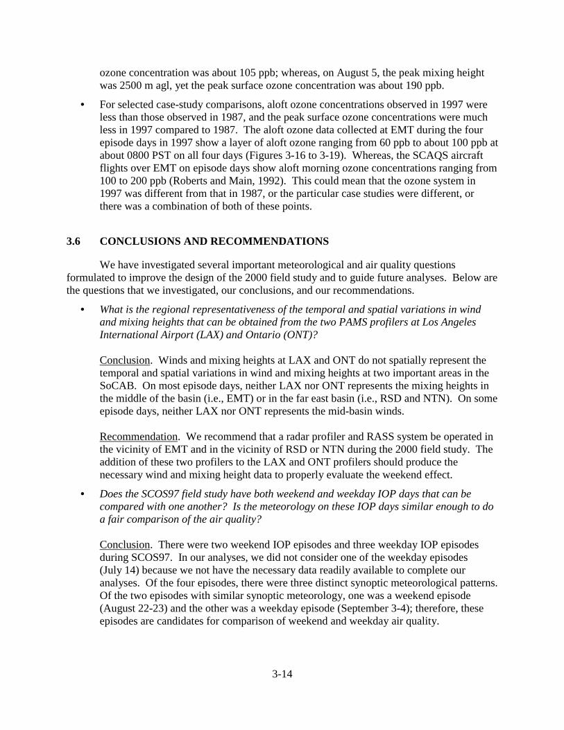
3-14

ozone concentration was about 105 ppb; whereas, on August 5, the peak mixing heightwas 2500 m agl, yet the peak surface ozone concentration was about 190 ppb.

• For selected case-study comparisons, aloft ozone concentrations observed in 1997 wereless than those observed in 1987, and the peak surface ozone concentrations were muchless in 1997 compared to 1987. The aloft ozone data collected at EMT during the fourepisode days in 1997 show a layer of aloft ozone ranging from 60 ppb to about 100 ppb atabout 0800 PST on all four days (Figures 3-16 to 3-19). Whereas, the SCAQS aircraftflights over EMT on episode days show aloft morning ozone concentrations ranging from100 to 200 ppb (Roberts and Main, 1992). This could mean that the ozone system in1997 was different from that in 1987, or the particular case studies were different, orthere was a combination of both of these points.

3.6 CONCLUSIONS AND RECOMMENDATIONS

We have investigated several important meteorological and air quality questionsformulated to improve the design of the 2000 field study and to guide future analyses. Below arethe questions that we investigated, our conclusions, and our recommendations.

• What is the regional representativeness of the temporal and spatial variations in windand mixing heights that can be obtained from the two PAMS profilers at Los AngelesInternational Airport (LAX) and Ontario (ONT)?

Conclusion. Winds and mixing heights at LAX and ONT do not spatially represent thetemporal and spatial variations in wind and mixing heights at two important areas in theSoCAB. On most episode days, neither LAX nor ONT represents the mixing heights inthe middle of the basin (i.e., EMT) or in the far east basin (i.e., RSD and NTN). On someepisode days, neither LAX nor ONT represents the mid-basin winds.

Recommendation. We recommend that a radar profiler and RASS system be operated inthe vicinity of EMT and in the vicinity of RSD or NTN during the 2000 field study. Theaddition of these two profilers to the LAX and ONT profilers should produce thenecessary wind and mixing height data to properly evaluate the weekend effect.

• Does the SCOS97 field study have both weekend and weekday IOP days that can becompared with one another? Is the meteorology on these IOP days similar enough to doa fair comparison of the air quality?

Conclusion. There were two weekend IOP episodes and three weekday IOP episodesduring SCOS97. In our analyses, we did not consider one of the weekday episodes(July 14) because we not have the necessary data readily available to complete ouranalyses. Of the four episodes, there were three distinct synoptic meteorological patterns.Of the two episodes with similar synoptic meteorology, one was a weekend episode(August 22-23) and the other was a weekday episode (September 3-4); therefore, theseepisodes are candidates for comparison of weekend and weekday air quality.

3-15

Recommendation. Because the meteorology of the ozone episodes is significantlydifferent on some days and because the different meteorological conditions may enhanceor degrade the weekend effect, modeling that attempts to understand the weekend effectmust be completed based on a number of meteorological conditions.

• What is the influence of the mixing heights and wind patterns on ozone concentrations?How similar are the SCOS97 episode days to the SCAQS 1987 episode days based on thecharacteristics of the aloft ozone layers?

Conclusion. The interaction among winds, mixing heights, and ozone concentrations istoo complex to form any definitive conclusions in this preliminary analysis about theirrelationship and how their relationship might influence the weekend effect. We foundthat the morning aloft ozone concentrations at EMT on selected 1997 episodes wereabout half the aloft ozone concentrations observed during selected 1987 episodes.Although the comparison was done with only a few days, the observation suggests thatcontribution of aloft ozone to surface ozone may not be as significant now as it was in1987.

Recommendation. We recommend a more detailed investigation of mixing heights,winds, and ozone concentrations in Phase II.

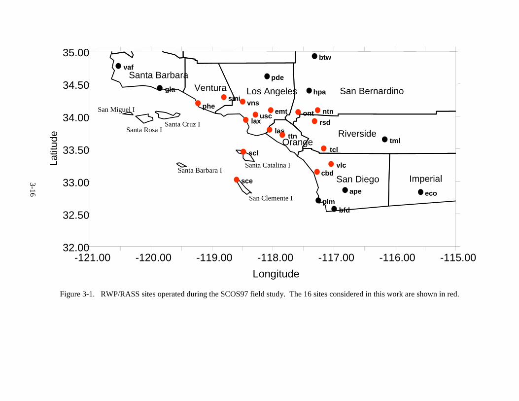
3-16

-121.00 -120.00 -119.00 -118.00 -117.00 -116.00 -115.00Longitude

32.00

32.50

33.00

33.50

34.00

34.50

35.00La

titud

e

ape

bfd

btw

cbd

eco

emt

gla hpa

laslax

ntnont

pde

phe

plm

rsd

sce

scl

smi

tcltmlttn

usc

vaf

vlc

vnsLos Angeles

San Diego

San Bernardino

RiversideOrange

VenturaSanta Barbara

Santa Catalina I

San Clemente I

Santa Barbara I

Santa Cruz ISanta Rosa I

San Miguel I

Imperial

Figure 3-1. RWP/RASS sites operated during the SCOS97 field study. The 16 sites considered in this work are shown in red.

3-17

0

500

1000

1500

2000

2500

3000

3500

4000

9/3/97 0:00 9/3/97 12:00 9/4/97 0:00 9/4/97 12:00 9/5/97 0:00

Time (PST)

Alti

tude

m a

gl

laxcbdlasphescesclsmittnusctclemtvns

Figure 3-2. Mixing height time-series plot for coastal and mid-basin sites in the SoCAB on September 3- 4, 1997.Coastal sites include LAX, CBD, SCE, and PHE.

3-18

0

500

1000

1500

2000

2500

3000

3500

4000

8/4 8/5 8/6 8/7 9/3 9/4 9/27 9/28 8/22 8/23

Date

Alti

tude

m a

gl

coastal averagemid-basin averageeast basin average

Note that for 8/22 and 8/23coastal avg. is only LAX, mid-basin avg. is only EMT, andeast-basin avg. is only RSD and ONT

Figure 3-3. Daily average peak mixing heights for coastal sites, mid-basin sites, and east-basin sites during four SCOS97 episodes.

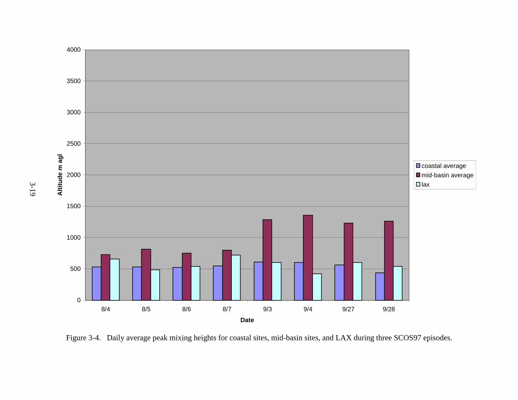
3-19

0

500

1000

1500

2000

2500

3000

3500

4000

8/4 8/5 8/6 8/7 9/3 9/4 9/27 9/28

Date

Alti

tude

m a

gl

coastal averagemid-basin averagelax

Figure 3-4. Daily average peak mixing heights for coastal sites, mid-basin sites, and LAX during three SCOS97 episodes.

3-20

0

500

1000

1500

2000

2500

3000

3500

4000

8/4 8/5 8/6 8/7 9/3 9/4 9/27 9/28Date

Alti

tude

m a

gl

mid-basin averageeast-basin averageont

Figure 3-5. Daily average peak mixing heights for mid-basin sites, east-basin sites, and ONT during three SCOS97 episodes.

3-21

0

500

1000

1500

2000

2500

3000

3500

4000

8/4 8/5 8/6 8/7 9/3 9/4 9/27 9/28

Date

Alti

tude

m a

gl

mid-basin averageemt

Figure 3-6. Daily average peak mixing heights for mid-basin sites and EMT during three SCOS97 episodes.

3-22

0

500

1000

1500

2000

2500

3000

3500

4000

8/4 8/5 8/6 8/7 9/3 9/4 9/27 9/28

Date

east-basin averagersd

Figure 3-7. Daily average peak mixing heights for east-basin sites and RSD during three SCOS97 episodes.

3-23

0 100200300400500600700800900Distances

PHE

SMI

VNS

EMTUSC

LAX

SCLSCE

LASTTN

ONT

NTNRSDTCL

VLC

CBD

Figure 3-8. Cluster analysis of daily peak mixing heights. The vertical lineis provided for discussion purposes. In general, the greater thedistance between variables joining a cluster, the less similar theirvariability.

3-24

y = 1.4956x - 72.579R2 = 0.5303

0

500

1000

1500

2000

2500

3000

3500

4000

4500

0 500 1000 1500 2000 2500 3000 3500 4000 4500

ONT hourly mixing height m agl

Figure 3-9. Scatter plot of hourly mixing heights from ONT and RSD duringthree SCOS97 episodes.

3-25

Figure 3-10. CALMET-derived winds (narrow arrows) and profiler-observed winds (bold arrows) at 500 m agl onSeptember 4, 1997, at 1500 PST.

3-26


3-27


3-28


3-29

Figure 3-14. National Weather Service daily weather map of 500-mb heights onAugust 5, 1997, at 0400 PST.

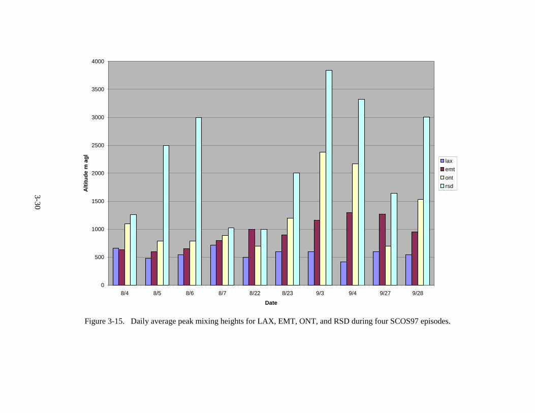
3-30

0

500

1000

1500

2000

2500

3000

3500

4000

8/4 8/5 8/6 8/7 8/22 8/23 9/3 9/4 9/27 9/28

Date

Alti

tude

m a

gl laxemtontrsd

Figure 3-15. Daily average peak mixing heights for LAX, EMT, ONT, and RSD during four SCOS97 episodes.

3-31

Figure 3-16. Time-height cross section of ozone concentrations by Lidar, profiler winds, and mixing heightsat EMT on August 4, 1997.

8 10 12 14 16 18 20 22

Time (PST)

500

1000

1500

2000

2500

Hei

ght (

m a

gl)

0 ppb

20 ppb

40 ppb

60 ppb

80 ppb

100 ppb

120 ppb

135 ppb

150 ppb

Wind Direction(South Wind, 3.5 m/s)

Mixing Height

3-32

Figure 3-17. Time-height cross section of ozone concentrations, profiler winds, and mixing heights at EMT on August 5, 1997.

8 10 12 14 16 18 20 22

Time (PST)

500

1000

1500

2000

2500H

eigh

t (m

agl

)

0 ppb

20 ppb

40 ppb

60 ppb

80 ppb

100 ppb

120 ppb

135 ppb

150 ppb


Mixing Height

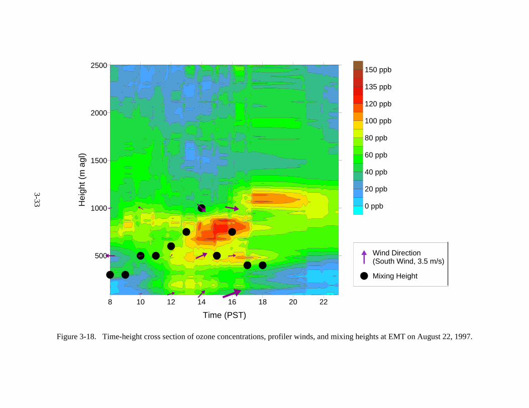
3-33


8 10 12 14 16 18 20 22

Time (PST)

500

1000

1500

2000

2500

Hei

ght (

m a

gl)

0 ppb

20 ppb

40 ppb

60 ppb

80 ppb

100 ppb

120 ppb

135 ppb

150 ppb


Mixing Height

3-34


4 6 8 10 12 14 16 18

Time (PST)

500

1000

1500

2000

2500

Hei

ght (

m a

gl)

0 ppb

20 ppb

40 ppb

60 ppb

80 ppb

100 ppb

120 ppb

135 ppb

150 ppb


Mixing Height

3-35

0

500

1000

1500

2000

2500

3000

3500

4000

4500

8/4/97 0:00 8/4/9712:00

8/5/97 0:00 8/5/9712:00

8/6/97 0:00 8/6/9712:00

8/7/97 0:00 8/7/9712:00

8/8/97 0:00

Time (PST)

Alti

tude

(m a

gl)

0

20

40

60

80

100

120

140

160

180

200

Ozo

ne c

once

ntra

tion

(ppb

)

Riverside mixing heightRubidoux ozone

Figure 3-20. Time-series plot of mixing heights at Riverside and surface ozone concentrations at Rubidoux on August 4-7, 1997.

3-36

Table 3-1. Radar wind profiler/RASS sites operated during the SCOS97 field study.The 16 sites considered in this work are shown in bold.

Site Name Site ID Latitude LongitudeElevation m msla

El Monte emt 34.09 118.03 95Norton ntn 34.09 117.26 318Alpine ape 32.86 116.81 463Brown Field bfd 32.57 116.99 158Carlsbad cbd 33.14 117.27 110El Centro eco 32.83 115.57 -18Goleta gla 34.43 119.85 4Los Alamitos las 33.79 118.05 7Palmdale pde 34.61 118.09 777Port Hueneme phe 34.17 119.22 2San Clemente Island sce 33.02 118.59 53Santa Catalina Island scl 33.45 118.48 37Tustin ttn 33.71 117.84 16Central Los Angeles usc 34.02 118.28 67Van Nuys vns 34.22 118.49 241Los Angeles Int. lax 33.94 118.44 47Ontario ont 34.06 117.58 280Point Loma plm 32.70 117.25 23Valley Center vlc 33.26 117.04 415Barstow btw 34.92 117.31 694Hesperia hpa 34.39 117.40 975Riverside rsd 33.92 117.31 488Temecula tcl 33.50 117.16 335Thermal tml 33.64 116.16 -36Vandenberg AFB vaf 34.77 120.53 149Simi Valley smi 34.29 118.80 279a msl = mean sea level

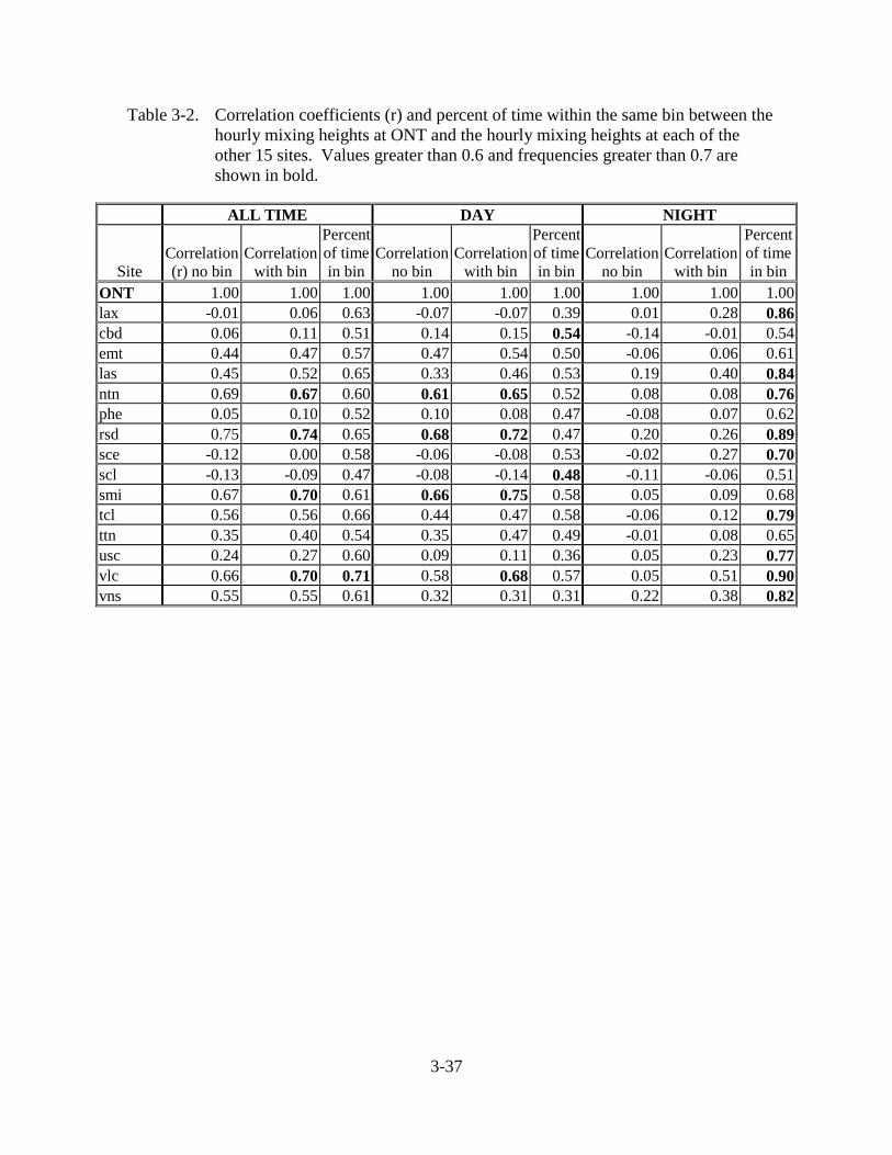
3-37

Table 3-2. Correlation coefficients (r) and percent of time within the same bin between thehourly mixing heights at ONT and the hourly mixing heights at each of theother 15 sites. Values greater than 0.6 and frequencies greater than 0.7 areshown in bold.

ALL TIME DAY NIGHT

SiteCorrelation(r) no bin

Correlationwith bin

Percentof timein bin

Correlationno bin

Correlationwith bin


Correlationno bin

Correlationwith bin


ONT 1.00 1.00 1.00 1.00 1.00 1.00 1.00 1.00 1.00lax -0.01 0.06 0.63 -0.07 -0.07 0.39 0.01 0.28 0.86cbd 0.06 0.11 0.51 0.14 0.15 0.54 -0.14 -0.01 0.54emt 0.44 0.47 0.57 0.47 0.54 0.50 -0.06 0.06 0.61las 0.45 0.52 0.65 0.33 0.46 0.53 0.19 0.40 0.84ntn 0.69 0.67 0.60 0.61 0.65 0.52 0.08 0.08 0.76phe 0.05 0.10 0.52 0.10 0.08 0.47 -0.08 0.07 0.62rsd 0.75 0.74 0.65 0.68 0.72 0.47 0.20 0.26 0.89sce -0.12 0.00 0.58 -0.06 -0.08 0.53 -0.02 0.27 0.70scl -0.13 -0.09 0.47 -0.08 -0.14 0.48 -0.11 -0.06 0.51smi 0.67 0.70 0.61 0.66 0.75 0.58 0.05 0.09 0.68tcl 0.56 0.56 0.66 0.44 0.47 0.58 -0.06 0.12 0.79ttn 0.35 0.40 0.54 0.35 0.47 0.49 -0.01 0.08 0.65usc 0.24 0.27 0.60 0.09 0.11 0.36 0.05 0.23 0.77vlc 0.66 0.70 0.71 0.58 0.68 0.57 0.05 0.51 0.90vns 0.55 0.55 0.61 0.32 0.31 0.31 0.22 0.38 0.82

3-38

Table 3-3. Correlation coefficients (r) and percent of time within the same bin betweenthe hourly mixing heights at LAX and the hourly mixing heights at each of theother 15 sites. Values greater than 0.6 and frequencies greater than 0.7 areshown in bold.

ALLTIME DAY NIGHT

SiteCorrelation(r) no bin

Correlationwith bin


Correlationno bin

Correlationwith bin


Correlationno bin

Correlationwith bin


LAX 1.00 1.00 1.00 1.00 1.00 1.00 1.00 1.00 1.00ont -0.01 0.04 0.63 -0.07 -0.06 0.40 0.01 0.41 0.87cbd -0.04 0.12 0.67 -0.27 0.07 0.65 0.12 0.22 0.69emt 0.07 0.12 0.63 -0.04 0.03 0.59 0.23 0.29 0.66las 0.01 0.08 0.68 -0.14 0.03 0.59 0.11 0.08 0.77ntn -0.04 -0.02 0.43 -0.12 -0.10 0.24 0.06 0.15 0.66phe 0.06 0.21 0.71 0.07 0.32 0.76 0.07 0.13 0.67rsd 0.05 0.04 0.52 0.02 0.01 0.27 -0.04 -0.09 0.76sce -0.11 0.10 0.69 -0.08 0.12 0.71 -0.13 0.10 0.67scl 0.04 0.09 0.64 0.01 0.13 0.67 0.10 0.09 0.62smi -0.01 0.04 0.58 -0.04 0.00 0.52 -0.04 0.14 0.62tcl 0.09 0.11 0.60 0.07 0.07 0.38 0.25 0.53 0.80ttn -0.05 0.01 0.59 -0.13 -0.02 0.53 -0.01 -0.01 0.65usc 0.01 0.06 0.59 -0.16 -0.09 0.47 0.17 0.23 0.71vlc -0.04 0.05 0.65 -0.09 -0.03 0.53 -0.14 0.20 0.77Vns 0.03 0.07 0.51 -0.03 -0.03 0.22 0.00 0.32 0.79

Table 3-4. SCOS97 IOP days used in this project (from Fujita et al., 1999).

Date Day of Week

Maximum 1-hr ozoneconcentration (ppb) in

the SoCAB

Maximum 8-hr ozoneconcentration (ppb) in

the SoCABAugust 4 Monday 140 105August 5 Tuesday 190 119August 6 Wednesday 160 125August 7 Thursday 150 122August 22 Friday 130 90August 23 Saturday 140 106

September 3 Wednesday 130 90September 4 Thursday 160 99September 5 Friday 120 91September 6 Saturday 120 94September 27 Saturday 140 102September 28 Sunday 170 107September 29 Monday 110 89

4-1

4. REFERENCES

California Air Resources Board (1998) Emission inventory 1996. Report prepared by theCalifornia Air Resources Board, Technical Support Division, Emission Inventory Branch,Sacramento, CA, July.

Dresser G. (1999) Personal communication. Texas Transportation Institute, College Station. TX,June.

Dye T.S., Lindsey C.G., Roberts P.T., and Anderson J.A. (1994) Evaluation of mixing depthsderived from 915 MHz radar profiler reflectivities during recent air quality studies. InPreprints of the Third International Symposium on Tropospheric Profiling: Needs andTechnologies, Hamburg, Germany, August 30-September 2, pp. 120-122.

Dye T.S., Roberts P.T., and MacDonald C.P. (1998) Mixing depth structure and evolution asdiagnosed from upper-air meteorological data collected during the NARSTO-Northeaststudy. Paper No. 5A.6 presented at the 10th Joint Conference on the Applications of AirPollution Meteorology, Phoenix, AZ, January 11-16 (STI 1749).

Fujita E.M., Croes B.E., Bennett C.L., Lawson D.R., Lurmann F.W., and Main H.H. (1992)Comparison of emission inventory and ambient concentration ratios of CO, NMOG, andNOx in California's South Coast Air Basin. J. Air & Waste Manag. Assoc. 42, 264-276.

Fujita E.M., Watson J.G., Chow J.C., and Lu Z. (1994) Validation of the chemical mass balancereceptor model applied to hydrocarbon source apportionment in the Southern CaliforniaAir Study. Environ. Sci. Technol. 28, 1633-1649.

Fujita E.M., Green M., Keislar R., Koracin D., Moosmuller H., and Watson J. (1999) SCOS97-NARSTO 1997 Southern California ozone study and aerosol study. Volume III: summaryof field study. Prepared for California Air Resources Board Research Division,Sacramento, CA by Energy & Environmental Engineering Center, Desert ResearchInstitute, Reno, NV, Contract No. 93-326, February.

Fujita E.M., Stockwell W., and Keislar R.E. (2000a) Weekend/weekday ozone observations inthe South Coast Air Basin, Phase I: retrospective analysis of ambient and emissions dataand refinement of hypotheses. Draft Report prepared for National Renewable EnergyLaboratory, Golden CO by Desert Research Institute, Reno NV, August 23.

Fujita E.M., Stockwell W., Keislar R.E., Campbell D.E., Roberts P.T., Funk T.H., McDonaldC.P., Main H.H., and Chinkin L.R. (2000b) Weekend/weekday ozone observations in theSouth Coast Air Basin: retrospective analysis of ambient and emissions data andrefinement of hypotheses, Volume I - Executive Summary. Prepared for NationalRenewable Energy Laboratory, Golden CO by Desert Research Institute, Reno NV andSonoma Technology, Inc., Petaluma CA, December 29.

Gertler A.W. and Pierson W.R. (1996) Recent measurements of mobile source emissionfactors in North American Tunnels. Science Total Environment 189-190, 107-113.

4-2

Glover E. and Brzezinski D. (1998a) Trip length activity factors for running loss and exhaustrunning emissions. Draft report prepared for the U.S. Environmental Protection Agency,Assessment and Modeling Division, Ann Arbor, MI, Report Number M6.FLT.005,February

Glover E. and Brzezinski D. (1998b) Soak length activity factors for hot soak emissions. Draftreport prepared for the U.S. Environmental Protection Agency, Assessment andModeling Division, Ann Arbor, MI, Report Number M6.FLT.004, February.

Guensler R. (1999) Personal communication. Georgia Institute of Technology, Atlanta GA June.

Haste T.L., Chinkin L.R. Main H.H., Kumar N., and Roberts P.T. (1998a) Analysis of Data fromthe 1995 NARSTO-Northeast Study Volume II: Use of PAMS Data to Evaluate aRegional Emission Inventory. Final report prepared for Coordinating Research Council,Atlanta, GA by Sonoma Technology, Inc., Petaluma, CA under subcontract to ENVIRONInternational Corp., Novato, CA, STI-95424-1737-FR, March.

Haste T.L., Chinkin L.R., Kumar N., Lurmann F.W., and Hurwitt S.B. (1998b) Use of AmbientData Collected During IMS-95 to Evaluate a Regional Emission Inventory for the SanJoaquin Valley. Final report prepared for San Joaquin Valleywide Air Pollution StudyAgency c/o California Air Resources Board, Sacramento, CA by Sonoma Technology,Inc., Petaluma, CA, STI-997211-1800-FR, July.

Holzworth G. (1972) Mixing heights, wind speeds, and potential for urban air pollutionthroughout the contiguous United States. Prepared by Office of Air Programs, U.S.Environmental Protection Agency, Research Triangle Park, NC, Publication No. AP-101.

Hsiao K. (1999) Personal communication. South Coast Air Quality Management District, LosAngeles, CA, June.

Korc M.E., Roberts P.T., Chinkin L.R., and Main H.H. (1993) Comparison of emissioninventory and ambient concentration ratios of CO, NMOC, and NOx in the LakeMichigan Air Quality Region. Draft final report prepared for Lake Michigan AirDirectors Consortium, Des Plaines, IL by Sonoma Technology, Inc., Santa Rosa, CA,STI-90218-1357-DFR, October.

Korc M.E., Roberts P.T., Chinkin L.R., Lurmann F.W., and Main H.H. (1995) Reconciliation ofemission inventory and ambient data for three major regional air quality studies. InTransactions - Regional Photochemical Measurement and Modeling Studies, pp. 176-194.

Lindsey C.G. and Dye T.S. (1994) Collecting and interpreting upper air data for the PAMSnetwork using radar profilers and RASS. Presented at the Air & Waste ManagementAssociation's Conference on Enhanced Ozone Monitoring: Status and Developments,International Symposium on Measurements of Toxic and Related Air Pollutants, Durham,NC, May 3-6.

4-3

MacDonald C.P., Roberts P.T., Main H.H., and Dye T.S. (1998) Phenomena that influence highozone concentrations in the Paso del Norte area. Paper presented at the Air and WasteManagement Association 1998 Annual Meeting and Exhibition, San Diego, CA, June 14-18.

MacDonald C.P., Knoderer C.A, Arndt R.L., Roberts P.T., Emery C., Stoeckenius T., and Tai E.(2000a) PAMS data analysis for Southern California Volume III: three-dimensional windfields and trajectories during three SCOS97 episodes. Draft final report prepared for theSouth Coast Air Quality Management District, Diamond Bar, CA by SonomaTechnology, Inc., Petaluma, CA and ENVIRON International, Inc., Novato, CA,STI-997526-1960-DFR, March.

MacDonald C.P., Dye T.S., Lilly M.A., and Roberts P.T. (2000b) PAMS data analysis forSouthern California Volume IV: surface-based mixing heights during three SCOS97episodes. Draft final report prepared for the South Coast Air Quality ManagementDistrict Diamond Bar, CA by Sonoma Technology, Inc. Petaluma, CA, STI-997527-1907-DFR, March.

Magbuhat S. and Long J.R. (1996) Improving California’s motor vehicle emissions inventoryactivity estimates through the use of data logger-equipped vehicles. In Proceedings of theSixth CRC On-Road Vehicle Emissions Workshop, San Diego, CA, March 18-20.Coordinating Research Council, Atlanta, GA.

Main H.H., Chinkin L.R., Chamberlin A.H., and Hyslop N.M. (1999) PAMS data analysis forSouthern California. Volume I: Characteristics of hydrocarbon data collected in theSouth Coast Air Quality Management District from 1994 to 1997. Report prepared forthe South Coast Air Quality Management District, Diamond Bar, CA by SonomaTechnology, Inc., Petaluma, CA, STI-997521-1899-DFR, September.

Niemeier D., Hicks J., Korve M., and Kim S. (1999) Estimation of allocation factors fordisaggregation of travel demand model volumes to hourly volumes for highways in theSouth Coast Air Basin. Part of the South Coast Air Basin Ozone Study. University ofCalifornia at Davis. Draft final report, March.

Roberts P.T. and Main H.H. (1992) Characterization of three-dimensional air quality during theSCAQS. In Southern California Air Quality Study Data Analysis. In Proceedings fromthe SCAQS Data Analysis Conference, University of California, Los Angeles, CA, July21-23, Air & Waste Management Association, Pittsburgh, PA, (STI-1223), VIP-26.

Roberts P.T., MacDonald C.P., Main H.H., Dye T.S., Coe D., and Haste T.L. (1997) Analysis ofmeteorological and air quality data for the 1996 Paso del Norte ozone study. Final reportprepared for U.S. Environmental Protection Agency, Region 6, Dallas TX undersubcontract to SAIC, McLean, VA by Sonoma Technology, Inc., Santa Rosa, CA,STI-997330-1754-FR, EPA Contract No. 68-D3-0030, Work Assignments III-102 andIII-130, September.

Wyngaard J.C. and LeMone M.A. (1980) Behavior of the refractive index structure parameter inthe entraining convective boundary layer. J. Atmos. Sci. 37, 1573-1585.

A-1

APPENDIX A

DESCRIPTION OF EMISSIONS ACTIVITY DATA

A. Dataset: Caltrans Weight In Motion (WIM) DatabaseSource: Caltrans maintained databaseDescription: Contains hourly and day-of-week vehicle counts for several vehicle classestraveling on freewaysVintage: 1998, Can request data for specific time periodSpatial Coverage: 4 sites located in Los Angeles county and 16 other sites throughout theSoCABRelevant Source Categories: All vehicle typesLimitations: Data collected on freeways only

B. Dataset: Vehicle counts on surface streetsSource: Collected by Deb NiemeierDescription: Contains hourly and day-of-week vehicle counts for several vehicle classes onsurface streets collected over a two-week time period (Sept. 30 – Oct. 13, 1997). CARB iscurrently obtaining electronic versions of all data.Vintage: 1997, HistoricalSpatial Coverage: Several sites, one located near L.A. North Main monitoring site, otherlocations unknown at this timeRelevant Source Categories: All vehicle typesLimitations: Data collected on surface streets only, two-week sampling period

C. Dataset: Heavy-duty diesel truck activity dataSource: Collected by Battelle/CARBDescription: Contains heavy-duty diesel activity data and route information.Approximately 140 heavy-duty diesel trucks fitted with GPS devices and tracked forspecified time periods in the state of California.Vintage: 1998, HistoricalSpatial Coverage: Includes regions of SoCAB but trucks travel in and out of SoCABthroughout CaliforniaRelevant Source Categories: Heavy-duty diesel trucksLimitations: Limited data may not be spatially adequate

A-2

D. Dataset: A&WMA paper reporting the development of a fuel-based emissions inventory forheavy-duty diesel trucksSource: David Dreher and Robert HarleyDescription: Reports development of a fuel-based emission inventory for heavy-duty dieseltrucks in the San Francisco Bay Area. Contains anecdotal discussion of truck activity onweekends versus weekdays.Vintage: 1998, HistoricalSpatial Coverage: Study conducted in San Francisco Bay AreaRelevant Source Categories: Heavy-duty diesel trucksLimitations: Anecdotal only

E. Dataset: Temporal, Spatial, and Ambient Temperature Effects in the Sacramento ModelingRegionSource: Study conducted by David Rocke and Daniel Chang at U.C. DavisDescription: Contains day-of-week and diurnal temporal profiles for select emissionscategoriesVintage: 1998Spatial Coverage: Emissions activity based on CaliforniaRelevant Source Categories: Heavy-duty diesel construction equipment, autobodyrefinishing, industrial and commercial adhesives and sealants, metal products and coatings.Limitations: Study done in Sacramento, but useful for representative profiles

F. Dataset: Driving behavior characteristics on weekdays and weekendsSource: Analyses done by Mark Carlock at CARBDescription: Summarizes driving behavior on weekdays and weekends including: VMT,vehicle speed distributions by day of week, gasoline sales by day-of-week, and fleet mixVintage: 1998Spatial Coverage: South Coast Air BasinRelevant Source Categories: Light-duty passenger vehiclesLimitations: None

G. Dataset: Improved emission inventory for pleasure craft in CaliforniaSource: Study done by Systems Applications InternationalDescription: Contains day-of-week and diurnal temporal profiles for pleasure craft inCalifornia.Vintage: 1995Spatial Coverage: CaliforniaRelevant Source Categories: Recreational boatsLimitations: None

H. Dataset: Los Angeles International Airport Flight SchedulesSource: LAX World Airport CenterDescription: Day-of-week flight activity for all flights arriving and departing at LAXVintage: Can obtain by request for specific time periodSpatial Coverage: LAXRelevant Source Categories: AirplanesLimitations: Limited to total flights

A-3

I. Dataset: Locomotive Emission Inventory, Supplement to the Locomotive Emission Study(April 1991)Source: Study done by Booz-Allen & Hamilton for CARBDescription: Contains average activity profiles by month and day-of-week for trains inCaliforniaVintage: 1992Spatial Coverage: California averagesRelevant Source Categories: TrainsLimitations: Slightly out of date, only contains California averages

J. Dataset: Ship dataSource: Marine Exchange L.A.-L.B. HarborDescription: Contains arrival and departure logs for all ships traveling into and out of LongBeach and Los Angeles harbors by day-of-week and hourVintage: Can request for specific time periodSpatial Coverage: Los Angeles and Long Beach harborsRelevant Source Categories: Marine vesselsLimitations: May have to pay for the data, approximately $50/month

K. Dataset: Heavy-duty Truck Population, Activity, and Usage PatternsSource: Report by Jack Faucett Associates for CARBDescription: Contains average heavy-duty diesel truck activity patterns such as VMT andspeed distribution. Also includes light-heavy and medium-heavy truck activity.Vintage: 1998Spatial Coverage: California average dataRelevant Source Categories: Heavy-, medium-, and light-duty diesel trucksLimitations: California average data, and nothing by day of week

L. Dataset: Hourly traffic count data collected during SCOS97Source: Study by Dr. Deb NiemeierDescription: Hourly traffic count data by day of week collected during SCOS97 for manysites throughout the SoCAB. Larry Larsen of CARB currently processing and analyzing thedata.Vintage: 1997Spatial Coverage: Many sites throughout SoCAB, Larry Larsen processing for relevantlocationsRelevant Source Categories: On-road vehiclesLimitations: Reports total vehicles only

WEEKDAY/WEEKEND OZONE OBSERVATIONS IN … · several government agencies and industry experts were ... Examples of daily traffic variation by type of ... CALMET-derived winds and

Documents