Tasks 5.2 and 6.3: The Influence of Winds Tasks 5.2 and 6.3: The Influence of Winds and Vertical Mixing on PM and Vertical Mixing on PM 2.5 2.5 Concentrations Concentrations Presented by: Presented by: Mark Lilly Mark Lilly Clinton MacDonald Clinton MacDonald Paul Roberts Paul Roberts Heather Arkinson Heather Arkinson Sonoma Technology, Inc. Sonoma Technology, Inc. Petaluma, CA Petaluma, CA Don Don Lehrman Lehrman Technical and Business Systems, Inc. Technical and Business Systems, Inc. Santa Rosa, CA Santa Rosa, CA Presented to: Presented to: CRPAQS Data Analysis Workshop CRPAQS Data Analysis Workshop Sacramento, CA Sacramento, CA March 9-10, 2004 March 9-10, 2004 902329-2504

Welcome message from author
This document is posted to help you gain knowledge. Please leave a comment to let me know what you think about it! Share it to your friends and learn new things together.
Transcript
1
Tasks 5.2 and 6.3: The Influence of WindsTasks 5.2 and 6.3: The Influence of Windsand Vertical Mixing on PMand Vertical Mixing on PM2.5 2.5 ConcentrationsConcentrations
Presented by:Presented by:Mark LillyMark Lilly
Clinton MacDonaldClinton MacDonaldPaul RobertsPaul Roberts
Heather ArkinsonHeather ArkinsonSonoma Technology, Inc.Sonoma Technology, Inc.
Petaluma, CAPetaluma, CA
Don Don LehrmanLehrmanTechnical and Business Systems, Inc.Technical and Business Systems, Inc.
Santa Rosa, CASanta Rosa, CA
Presented to:Presented to:CRPAQS Data Analysis WorkshopCRPAQS Data Analysis Workshop
Sacramento, CASacramento, CAMarch 9-10, 2004March 9-10, 2004
902329-2504

2
Task 5.2: Evaluation of TransportTask 5.2: Evaluation of Transport•• WindsWinds
–– Transport pathwaysTransport pathways–– Flows: nocturnal jet, eddy, terrainFlows: nocturnal jet, eddy, terrain–– Flux planesFlux planes–– Advection vs. diffusionAdvection vs. diffusion
•• Mixing heightsMixing heights•• Synoptic weatherSynoptic weather
–– WindsWinds–– MixingMixing

3
Task 6.3: Transport and the RegionalTask 6.3: Transport and the RegionalNature of Secondary PMNature of Secondary PM
•• Causes of the regional nature of PMCauses of the regional nature of PM–– TransportTransport–– DiffusionDiffusion–– Emission source locationEmission source location–– Aloft Aloft NONOxx emissions emissions
4
ApproachApproach•• CALMET modelingCALMET modeling
–– Wind fieldsWind fields–– TrajectoriesTrajectories–– Dispersion (CALPUFF)Dispersion (CALPUFF)
•• Data AnalysisData Analysis–– Profiler windsProfiler winds–– Mixing heightsMixing heights–– PM dataPM data
•• Case StudiesCase Studies–– November 17 through 26, 2000November 17 through 26, 2000–– December 13 through 20, 2000December 13 through 20, 2000–– December 24 through 30, 2000December 24 through 30, 2000–– January 2 through 9, 2001January 2 through 9, 2001
5
CALMET – BackgroundCALMET – Background
•• What is CALMET?What is CALMET?–– A meteorological model that includes a diagnosticA meteorological model that includes a diagnostic
wind field generator containing objective analysis andwind field generator containing objective analysis andparameterized treatments of slope flows, parameterized treatments of slope flows, kinematickinematicterrain effects, terrain-blocking effects, a divergenceterrain effects, terrain-blocking effects, a divergenceminimization procedure, and a micro-meteorologicalminimization procedure, and a micro-meteorologicalmodel for overland and model for overland and overwateroverwater boundary layers boundary layers
•• Why use CALMET?Why use CALMET?–– To resolve To resolve mesoscalemesoscale and local-scale meteorological and local-scale meteorological
phenomena by blending observational data withphenomena by blending observational data withsynoptic-scale model results and analysessynoptic-scale model results and analyses
6
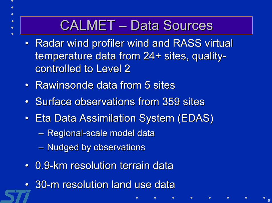
CALMET – Data SourcesCALMET – Data Sources•• Radar wind profiler wind and RASS virtualRadar wind profiler wind and RASS virtual
temperature data from 24+ sites, quality-temperature data from 24+ sites, quality-controlled to Level 2controlled to Level 2
•• RawinsondeRawinsonde data from 5 sites data from 5 sites•• Surface observations from 359 sitesSurface observations from 359 sites•• EtaEta Data Assimilation System (EDAS) Data Assimilation System (EDAS)
–– Regional-scale model dataRegional-scale model data–– Nudged by observationsNudged by observations
•• 0.9-km resolution terrain data0.9-km resolution terrain data
•• 30-m resolution land use data30-m resolution land use data

7
CALMET – Data sitesCALMET – Data sitesUpper-air Surface
8
CALMET CALMET –– Grid Resolution Grid Resolution
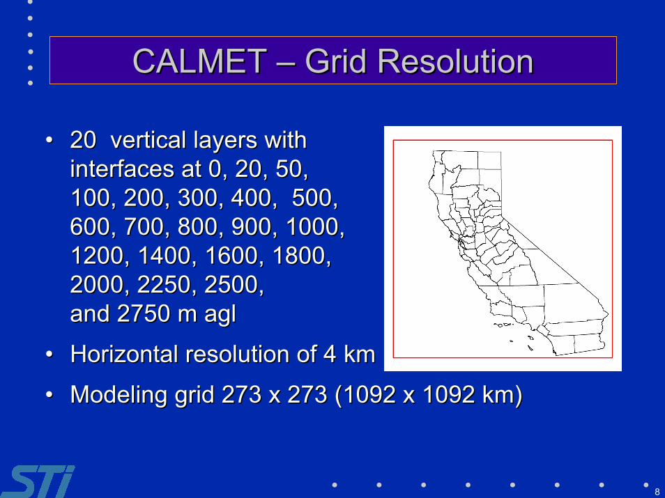
•• 20 vertical layers with20 vertical layers withinterfaces at 0, 20, 50,interfaces at 0, 20, 50,100, 200, 300, 400, 500,100, 200, 300, 400, 500,600, 700, 800, 900, 1000,600, 700, 800, 900, 1000,1200, 1400, 1600, 1800,1200, 1400, 1600, 1800,2000, 2250, 2500,2000, 2250, 2500,and 2750 m and 2750 m aglagl
•• Horizontal resolution of 4 kmHorizontal resolution of 4 km
•• Modeling grid 273 x 273 (1092 x 1092 km)Modeling grid 273 x 273 (1092 x 1092 km)

9
CALMETCALMET –– Method MethodNormal
First guess wind at all grid pointscreated using data at only one
location and height
Blend EDAS and observationusing weighting factors
Smooth
Intermediate winds
Terrain effects
First guess
Blend with observations and grid
Smooth (optional)
Final winds
CRPAQS
Terrain effects
Blend with observations and grid
Smooth (optional)
Final winds

10
Data Analysis Data Analysis –– Case Study: Case Study:Focus on December 22-31, 2000Focus on December 22-31, 2000
•• Synoptic WeatherSynoptic Weather•• Mixing DepthMixing Depth
–– PeakPeak–– Diurnal cycleDiurnal cycle–– Spatial distributionSpatial distribution
•• WindsWinds–– EddiesEddies–– JetsJets–– Terrain flowsTerrain flows
•• TransportTransport–– Distance, direction, speedDistance, direction, speed

11
Mixing Depth Mixing Depth –– Definition Definition
RL = Residual LayerCBL = Convective Boundary LayerNBL = Nocturnal Boundary LayerMBL = Marine Boundary Layer
Midnight
NBL NBL
CBL RLRL
Subsidence Inversion
Sunrise Sunset
Hei
ght
MBL
= Surface-based vertical mixing
= Surface-based mixing depth
12
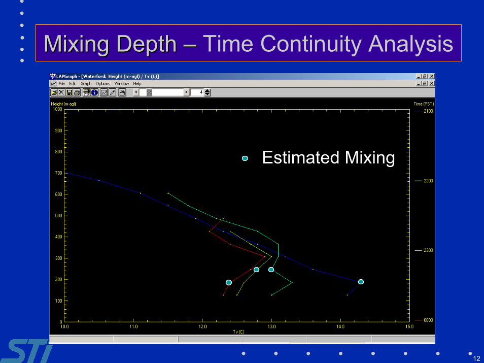
Mixing Depth – Mixing Depth – Time Continuity Analysis
Estimated Mixing

13
Mixing Depth Mixing Depth –– December 22-31, 2000 December 22-31, 2000Hourly Mixing Heights
December 22 to 31, 2000
0
200
400
600
800
1000
1200
1400
1600
12/22
/2000
00:00
12/22
/2000
12:00
12/23
/2000
00:00
12/23
/2000
12:00
12/24
/2000
00:00
12/24
/2000
12:00
12/25
/2000
00:00
12/25
/2000
12:00
12/26
/2000
00:00
12/26
/2000
12:00
12/27
/2000
00:00
12/27
/2000
12:00
12/28
/2000
00:00
12/28
/2000
12:00
12/29
/2000
00:00
12/29
/2000
12:00
12/30
/2000
00:00
12/30
/2000
12:00
12/31
/2000
00:00
12/31
/2000
12:00
Date and Time (PST)
Mix
ing
Hei
ght (
m a
gl)
AngiolaBakersfieldChowchilla
14
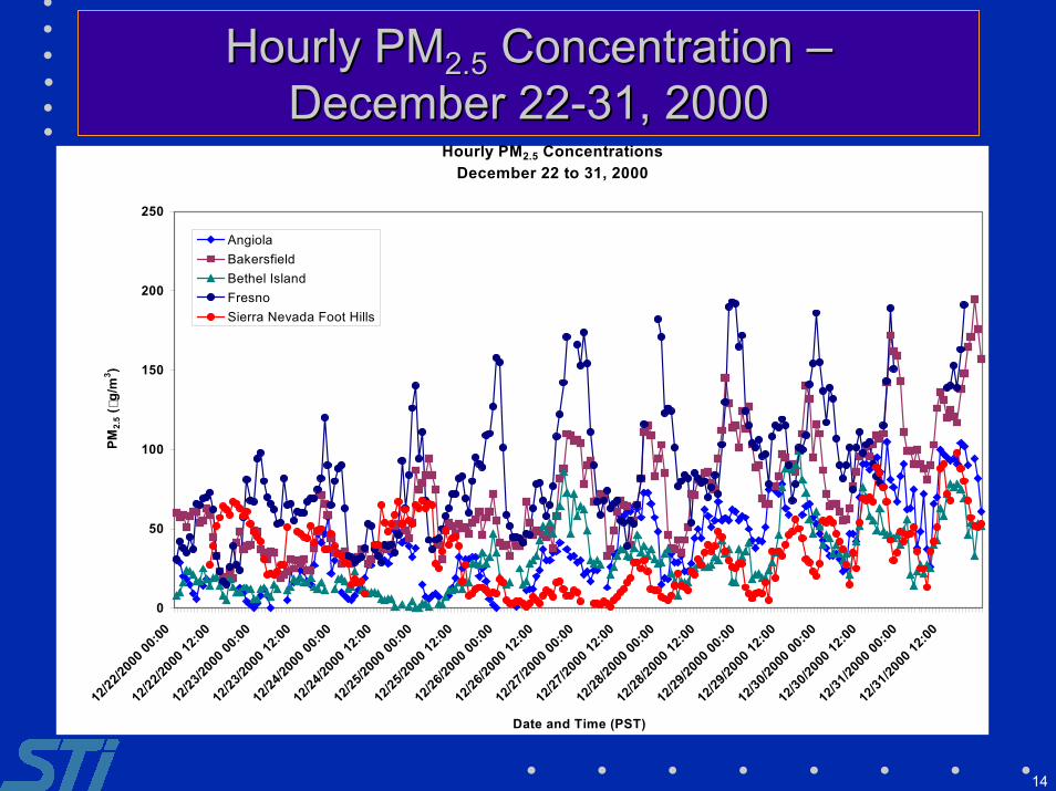
Hourly PMHourly PM2.52.5 Concentration Concentration ––December 22-31, 2000December 22-31, 2000
Hourly PM2.5 ConcentrationsDecember 22 to 31, 2000
0
50
100
150
200
250
12/22
/2000
00:00
12/22
/2000
12:00
12/23
/2000
00:00
12/23
/2000
12:00
12/24
/2000
00:00
12/24
/2000
12:00
12/25
/2000
00:00
12/25
/2000
12:00
12/26
/2000
00:00
12/26
/2000
12:00
12/27
/2000
00:00
12/27
/2000
12:00
12/28
/2000
00:00
12/28
/2000
12:00
12/29
/2000
00:00
12/29
/2000
12:00
12/30
/2000
00:00
12/30
/2000
12:00
12/31
/2000
00:00
12/31
/2000
12:00
Date and Time (PST)
PM2.
5 (g/
m3 )
AngiolaBakersfieldBethel IslandFresnoSierra Nevada Foot Hills

15
SynopticsSynoptics –– 500- 500-mbmb Heights Heights
December 24, 2000 December 28, 2000
16
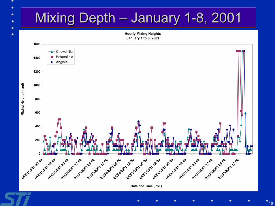
Mixing Depth Mixing Depth –– January 1-8, 2001 January 1-8, 2001Hourly Mixing HeightsJanuary 1 to 6, 2001
0
200
400
600
800
1000
1200
1400
1600
01/01
/2001
00:00
01/01
/2001
12:00
01/02
/2001
00:00
01/02
/2001
12:00
01/03
/2001
00:00
01/03
/2001
12:00
01/04
/2001
00:00
01/04
/2001
12:00
01/05
/2001
00:00
01/05
/2001
12:00
01/06
/2001
00:00
01/06
/2001
12:00
01/07
/2001
00:00
01/07
/2001
12:00
01/08
/2001
00:00
01/08
/2001
12:00
Date and Time (PST)
Mix
ing
Hei
ght (
m a
gl)
ChowchillaBakersfieldAngiola

17
Mixing Depth Mixing Depth –– December 27 and 28, 2000 December 27 and 28, 2000Hourly Mixing Heights
December 27 and 28, 2000
0
100
200
300
400
500
600
700
800
12:0
0:00
AM
1:00
:00
AM
2:00
:00
AM
3:00
:00
AM
4:00
:00
AM
5:00
:00
AM
6:00
:00
AM
7:00
:00
AM
8:00
:00
AM
9:00
:00
AM
10:0
0:00
AM
11:0
0:00
AM
12:0
0:00
PM
1:00
:00
PM2:
00:0
0 PM
3:00
:00
PM4:
00:0
0 PM
5:00
:00
PM6:
00:0
0 PM
7:00
:00
PM8:
00:0
0 PM
9:00
:00
PM10
:00:
00 P
M11
:00:
00 P
M12
:00:
00 A
M1:
00:0
0 A
M2:
00:0
0 A
M3:
00:0
0 A
M4:
00:0
0 A
M5:
00:0
0 A
M6:
00:0
0 A
M7:
00:0
0 A
M8:
00:0
0 A
M9:
00:0
0 A
M10
:00:
00 A
M11
:00:
00 A
M12
:00:
00 P
M1:
00:0
0 PM
2:00
:00
PM3:
00:0
0 PM
4:00
:00
PM5:
00:0
0 PM
6:00
:00
PM7:
00:0
0 PM
8:00
:00
PM9:
00:0
0 PM
10:0
0:00
PM
11:0
0:00
PM
12/27/00 12/28/00
Date and Time (PST)
Mix
ing
Hei
ght (
m a
gl)
ANGBSECHO
18
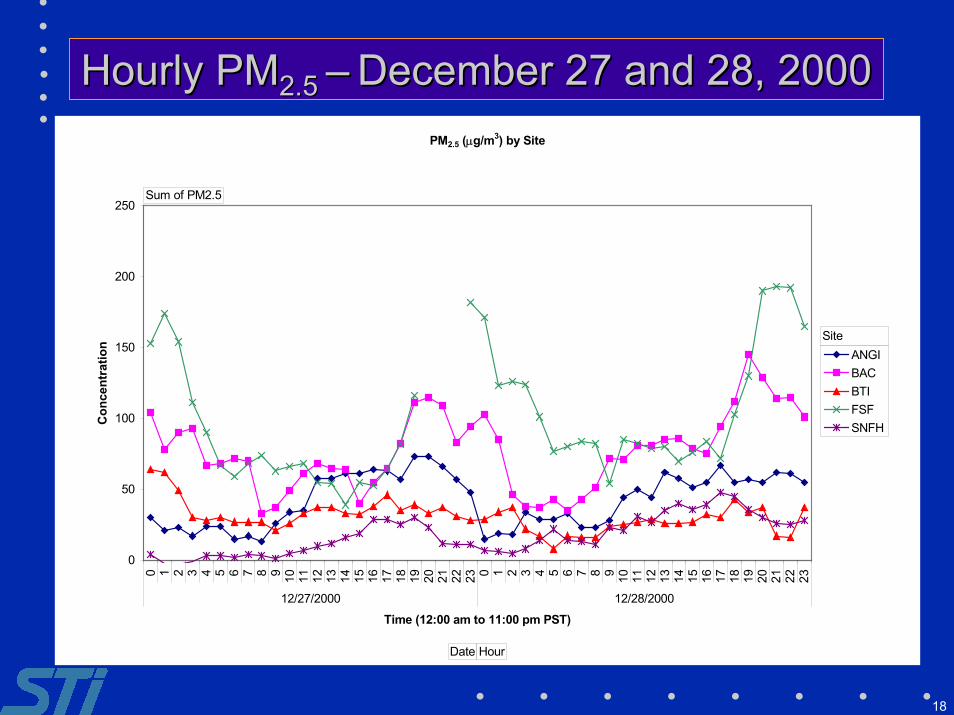
Hourly PMHourly PM2.5 2.5 –– December 27 and 28, 2000December 27 and 28, 2000
Insert PM time series
PM2.5 (µg/m3) by Site
0
50
100
150
200
250
0 1 2 3 4 5 6 7 8 9 10 11 12 13 14 15 16 17 18 19 20 21 22 23 0 1 2 3 4 5 6 7 8 9 10 11 12 13 14 15 16 17 18 19 20 21 22 23
12/27/2000 12/28/2000
Time (12:00 am to 11:00 pm PST)
Con
cent
ratio
n
ANGIBACBTIFSFSNFH
Sum of PM2.5
Date Hour
Site
19
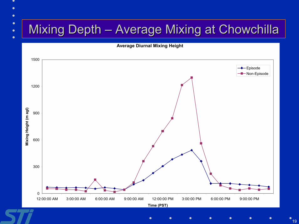
Mixing DepthMixing Depth – Average Mixing at Chowchilla – Average Mixing at ChowchillaAverage Diurnal Mixing Height
0
300
600
900
1200
1500
12:00:00 AM 3:00:00 AM 6:00:00 AM 9:00:00 AM 12:00:00 PM 3:00:00 PM 6:00:00 PM 9:00:00 PM
Time (PST)
Mix
ing
Hei
ght (
m a
gl)
EpisodeNon-Episode

20
Mixing DepthMixing Depth – Average Mixing at Bakersfield – Average Mixing at Bakersfield
Average Diurnal Mixing Height
0
300
600
900
1200
1500
12:00:00 AM 3:00:00 AM 6:00:00 AM 9:00:00 AM 12:00:00 PM 3:00:00 PM 6:00:00 PM 9:00:00 PM
Time (PST)
Mix
ing
Hei
ght (
m a
gl)
EpisodeNon-Episode

21
Winds Winds –– 10 m on December 26 at 1500 PST 10 m on December 26 at 1500 PST

22
Winds – 10 m on December 27 at 1500 PSTWinds – 10 m on December 27 at 1500 PST

23
Winds – 450 m on December 27 at 1500 PSTWinds – 450 m on December 27 at 1500 PST
24
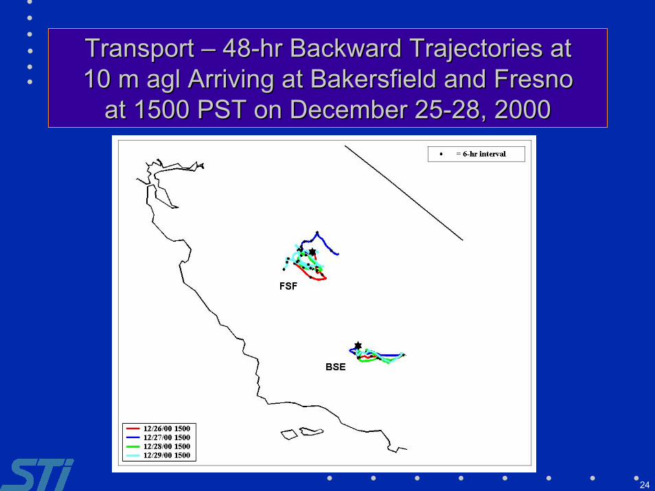
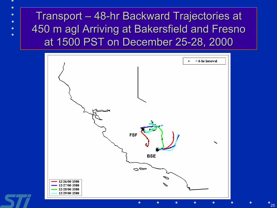
Transport Transport –– 48-hr Backward Trajectories at48-hr Backward Trajectories at10 m 10 m aglagl Arriving at Bakersfield and Fresno Arriving at Bakersfield and Fresno
at 1500 PST on December 25-28, 2000at 1500 PST on December 25-28, 2000
25
Transport Transport –– 48-hr Backward Trajectories at48-hr Backward Trajectories at450 m 450 m aglagl Arriving at Bakersfield and Fresno Arriving at Bakersfield and Fresno
at 1500 PST on December 25-28, 2000at 1500 PST on December 25-28, 2000
26
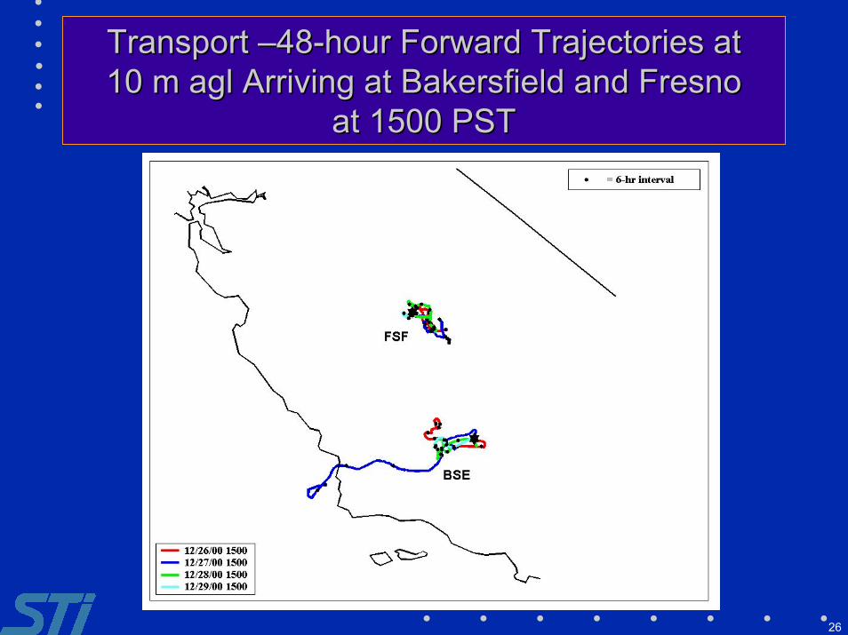
Transport Transport ––48-hour Forward Trajectories at48-hour Forward Trajectories at10 m 10 m aglagl Arriving at Bakersfield and Fresno Arriving at Bakersfield and Fresno
at 1500 PSTat 1500 PST

27
Transport: 48-hr Forward Trajectories at 450 mTransport: 48-hr Forward Trajectories at 450 maglagl Arriving at BAK and FSF at 1500 PST Arriving at BAK and FSF at 1500 PST
28
0
45
90
135
180
225
270
315
Bsp (inverse Mm)>0 - 50
>50 - 100
>100 - 200
>200 - 300
>300 - 400
>400
0% 4% 8% 12% 16% 20%
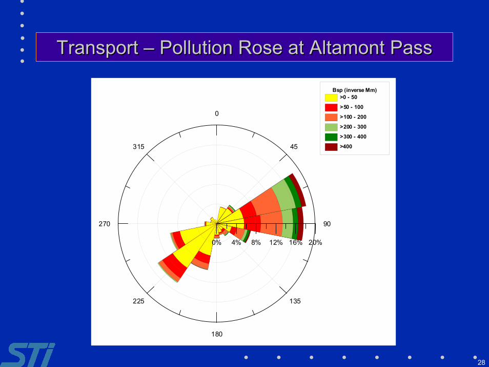
Transport Transport –– Pollution Rose at Altamont Pass Pollution Rose at Altamont Pass
29
0
45
90
135
180
225
270
315
Bsp (inverse Mm)>0 - 50
>50 - 100
>100 - 200
>200 - 300
>300 - 400
>400
0% 10% 20% 30%
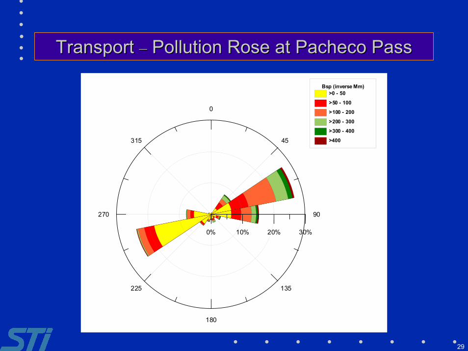
Transport Transport –– Pollution Rose at Pacheco Pass Pollution Rose at Pacheco Pass
30
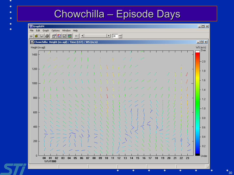
Chowchilla Chowchilla –– Episode Days Episode Days
31
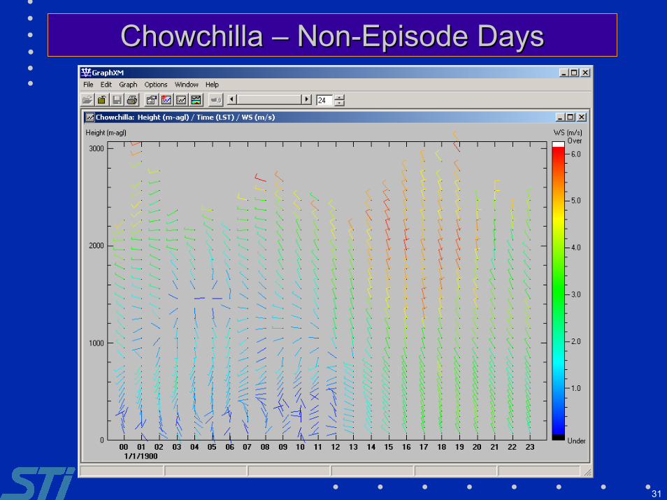
Chowchilla Chowchilla –– Non-Episode Days Non-Episode Days
32
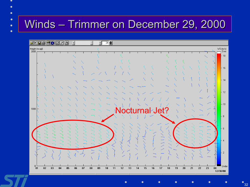
Winds Winds –– Trimmer on December 29, 2000 Trimmer on December 29, 2000
Nocturnal Jet?
33
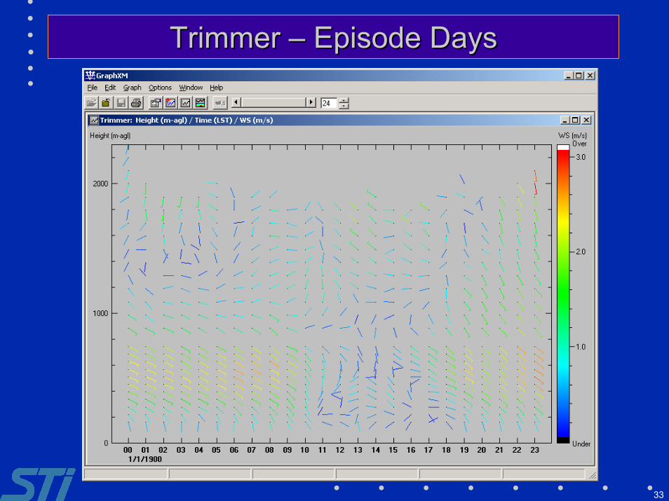
Trimmer Trimmer –– Episode Days Episode Days
34
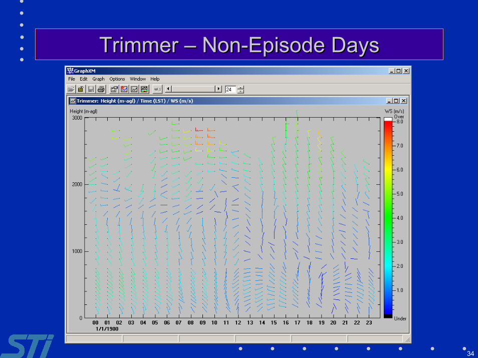
Trimmer Trimmer –– Non-Episode Days Non-Episode Days
35
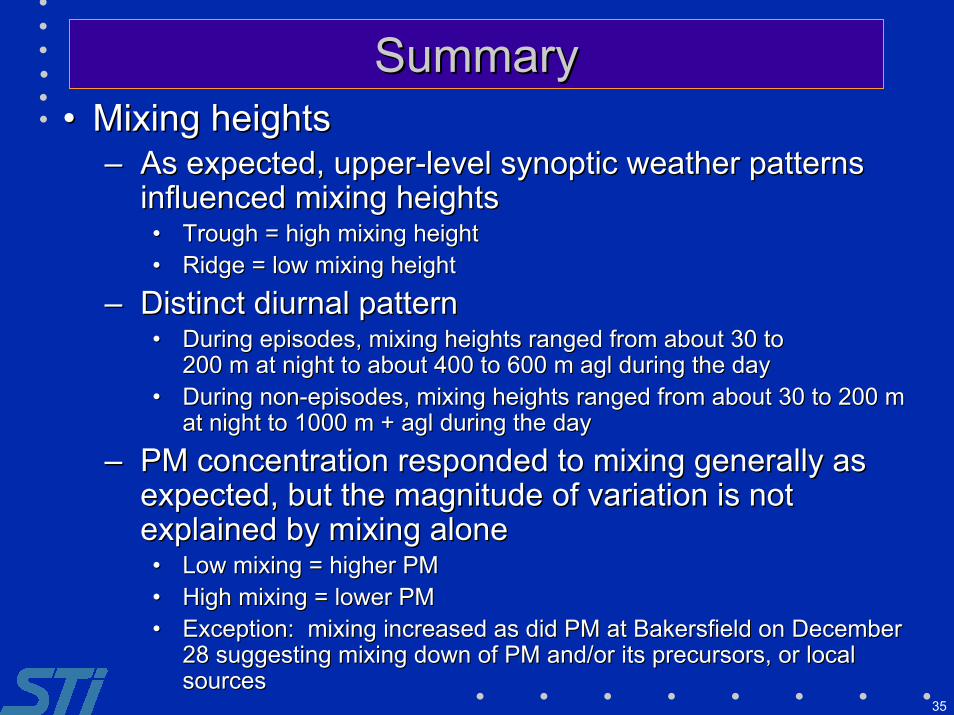
SummarySummary•• Mixing heightsMixing heights
–– As expected, upper-level synoptic weather patternsAs expected, upper-level synoptic weather patternsinfluenced mixing heightsinfluenced mixing heights•• Trough = high mixing heightTrough = high mixing height•• Ridge = low mixing heightRidge = low mixing height
–– Distinct diurnal patternDistinct diurnal pattern•• During episodes, mixing heights ranged from about 30 toDuring episodes, mixing heights ranged from about 30 to
200 m at night to about 400 to 600 m 200 m at night to about 400 to 600 m aglagl during the day during the day•• During non-episodes, mixing heights ranged from about 30 to 200 mDuring non-episodes, mixing heights ranged from about 30 to 200 m
at night to 1000 m + at night to 1000 m + aglagl during the day during the day
–– PM concentration responded to mixing generally asPM concentration responded to mixing generally asexpected, but the magnitude of variation is notexpected, but the magnitude of variation is notexplained by mixing aloneexplained by mixing alone•• Low mixing = higher PMLow mixing = higher PM•• High mixing = lower PMHigh mixing = lower PM•• Exception: mixing increased as did PM at Bakersfield on DecemberException: mixing increased as did PM at Bakersfield on December
28 suggesting mixing down of PM and/or its precursors, or local28 suggesting mixing down of PM and/or its precursors, or localsourcessources

36
SummarySummary•• WindsWinds
–– Episodes had lighter winds during the day than didEpisodes had lighter winds during the day than didnon-episodesnon-episodes
–– During episodesDuring episodes•• Winds were variable in direction and were generally lightWinds were variable in direction and were generally light
from the surface to the maximum daytime mixing height offrom the surface to the maximum daytime mixing height ofabout 500 m about 500 m aglagl, and at times much higher., and at times much higher.
•• There is no evidence of transport from the San FranciscoThere is no evidence of transport from the San FranciscoBay Area (Bay Area (SFBASFBA) into the San Joaquin Valley () into the San Joaquin Valley (SJVSJV) during) duringepisodesepisodes
•• There is evidence of transport from the SJV into the There is evidence of transport from the SJV into the SFBASFBA..•• We have not reached conclusions about transport from theWe have not reached conclusions about transport from the
Sacramento Valley into the SJV or visa versa.Sacramento Valley into the SJV or visa versa.
37
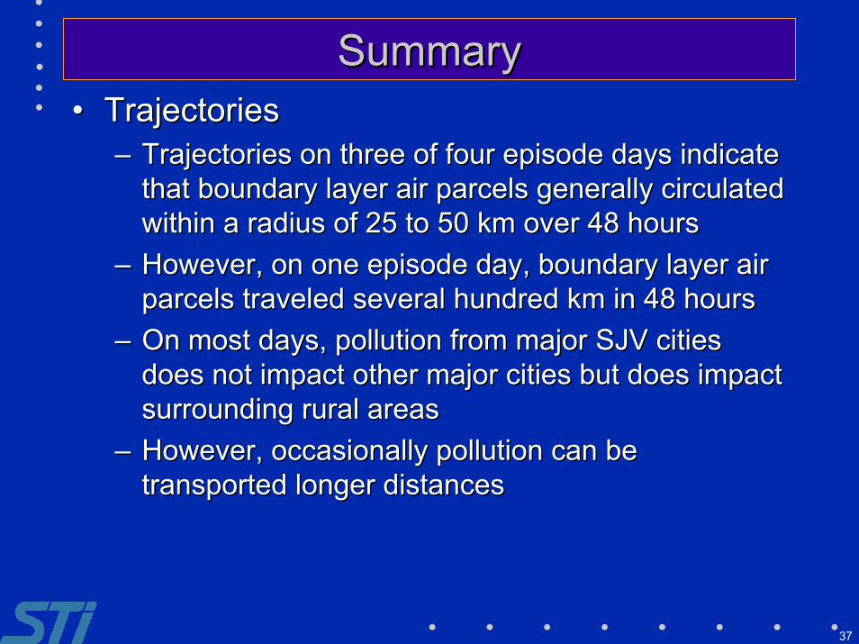
SummarySummary•• TrajectoriesTrajectories
–– Trajectories on three of four episode days indicateTrajectories on three of four episode days indicatethat boundary layer air parcels generally circulatedthat boundary layer air parcels generally circulatedwithin a radius of 25 to 50 km over 48 hourswithin a radius of 25 to 50 km over 48 hours
–– However, on one episode day, boundary layer airHowever, on one episode day, boundary layer airparcels traveled several hundred km in 48 hoursparcels traveled several hundred km in 48 hours
–– On most days, pollution from major On most days, pollution from major SJVSJV cities citiesdoes not impact other major cities but does impactdoes not impact other major cities but does impactsurrounding rural areassurrounding rural areas
–– However, occasionally pollution can beHowever, occasionally pollution can betransported longer distancestransported longer distances

38
What’s NextWhat’s Next•• Complete modeling of other episodesComplete modeling of other episodes•• Run additional trajectoriesRun additional trajectories•• Perform CALPUFF dispersion modelingPerform CALPUFF dispersion modeling•• Integrate findings from other episodes intoIntegrate findings from other episodes into
existing resultsexisting results•• Further analyze regional chemicalFurther analyze regional chemical
characterization of secondary PMcharacterization of secondary PM•• Deliver results for integration into other tasksDeliver results for integration into other tasks
Related Documents