Politecnico di Torino Department of Mechanical and Aerospace Engineering Master of Science degree in Mechanical Engineering Master of Science Thesis Radial turbine geometrical parameters optimization based on CFD analysis and application to engine performance assessment Mentors Prof. Mirko Baratta Prof. Dmytro Samoilenko Candidate Andrea Occhipinti April 2019

Welcome message from author
This document is posted to help you gain knowledge. Please leave a comment to let me know what you think about it! Share it to your friends and learn new things together.
Transcript
Politecnico di Torino
Department of Mechanical and Aerospace EngineeringMaster of Science degree in Mechanical Engineering
Master of Science Thesis
Radial turbine geometrical parameters optimization based onCFD analysis and application to engine performance assessment
Mentors
Prof. Mirko BarattaProf. Dmytro Samoilenko
Candidate
Andrea Occhipinti
April 2019

Dedicated to my family,for all their support and inspiration


Statement
As author of the thesis entitled:
Radial turbine geometrical parameters optimization based on CFD analysis and
application to engine performance assessment
which I have done myself, observing the rules of intellectual property protection, I allow my
work to be made public and I agree to make it available in the Library of the Faculty of
Automotive and Construction Machinery Engineering of the Warsaw University of Technology
as part of the statutory tasks of the library.
3
Contents
Abstract 13
1 Introduction 14
1.1 Background . . . . . . . . . . . . . . . . . . . . . . . . . . . . . . . . . . . . . . 14
1.2 Turbocharger fundamentals . . . . . . . . . . . . . . . . . . . . . . . . . . . . . 15
1.2.1 Working principle . . . . . . . . . . . . . . . . . . . . . . . . . . . . . . 15
1.2.2 Compressor side . . . . . . . . . . . . . . . . . . . . . . . . . . . . . . . 16
1.2.3 Turbine side . . . . . . . . . . . . . . . . . . . . . . . . . . . . . . . . . . 17
1.3 Turbocharging techniques . . . . . . . . . . . . . . . . . . . . . . . . . . . . . . 19
1.4 CFD analysis software . . . . . . . . . . . . . . . . . . . . . . . . . . . . . . . . 21
1.4.1 SOLIDWORKS FloXpressTM . . . . . . . . . . . . . . . . . . . . . . . . 22
1.4.2 SOLIDWORKS Flow SimulationTM . . . . . . . . . . . . . . . . . . . . 22
1.4.3 GT-POWER SuiteTM . . . . . . . . . . . . . . . . . . . . . . . . . . . . 22
2 Literature review 23
2.1 Radial turbine theory . . . . . . . . . . . . . . . . . . . . . . . . . . . . . . . . 23
2.1.1 Governing equations . . . . . . . . . . . . . . . . . . . . . . . . . . . . . 23
2.1.2 Fluid specific work . . . . . . . . . . . . . . . . . . . . . . . . . . . . . . 27
2.1.3 Volute . . . . . . . . . . . . . . . . . . . . . . . . . . . . . . . . . . . . . 27
2.2 Solidworks - Computational architecture . . . . . . . . . . . . . . . . . . . . . . 28
2.2.1 Governing equations . . . . . . . . . . . . . . . . . . . . . . . . . . . . . 28
2.2.2 Laminar/turbulent boundary model . . . . . . . . . . . . . . . . . . . . 29
2.2.3 Mesh . . . . . . . . . . . . . . . . . . . . . . . . . . . . . . . . . . . . . . 29
2.3 GT-Power model implementation . . . . . . . . . . . . . . . . . . . . . . . . . . 31
2.3.1 Maps evaluation . . . . . . . . . . . . . . . . . . . . . . . . . . . . . . . 32
3 Model description 34
4
CONTENTS
3.1 Geometry overview . . . . . . . . . . . . . . . . . . . . . . . . . . . . . . . . . . 34
3.1.1 Wheel’s trim . . . . . . . . . . . . . . . . . . . . . . . . . . . . . . . . . 35
3.1.2 Turbine housing A/R . . . . . . . . . . . . . . . . . . . . . . . . . . . . 36
3.2 Reference data . . . . . . . . . . . . . . . . . . . . . . . . . . . . . . . . . . . . 38
4 SolidWorks simulation setup 39
4.1 Computational domain creation . . . . . . . . . . . . . . . . . . . . . . . . . . . 39
4.1.1 Fluid check . . . . . . . . . . . . . . . . . . . . . . . . . . . . . . . . . . 40
4.2 FloXpress pre-analysis . . . . . . . . . . . . . . . . . . . . . . . . . . . . . . . . 40
4.2.1 Result . . . . . . . . . . . . . . . . . . . . . . . . . . . . . . . . . . . . . 41
4.3 Flow Simulation . . . . . . . . . . . . . . . . . . . . . . . . . . . . . . . . . . . 42
4.3.1 Analysis type . . . . . . . . . . . . . . . . . . . . . . . . . . . . . . . . . 42
4.3.2 Fluid . . . . . . . . . . . . . . . . . . . . . . . . . . . . . . . . . . . . . . 43
4.3.3 Wall and initial conditions . . . . . . . . . . . . . . . . . . . . . . . . . . 44
4.3.4 Computational domain and mesh . . . . . . . . . . . . . . . . . . . . . . 44
4.3.5 Boundary conditions . . . . . . . . . . . . . . . . . . . . . . . . . . . . . 45
4.3.6 Goals & convergence . . . . . . . . . . . . . . . . . . . . . . . . . . . . . 46
5 SolidWorks - Calculations 47
5.1 Methodology . . . . . . . . . . . . . . . . . . . . . . . . . . . . . . . . . . . . . 47
5.2 Results . . . . . . . . . . . . . . . . . . . . . . . . . . . . . . . . . . . . . . . . . 48
5.2.1 Fluid - Air . . . . . . . . . . . . . . . . . . . . . . . . . . . . . . . . . . 49
5.2.2 Fluid - Exhaust gas . . . . . . . . . . . . . . . . . . . . . . . . . . . . . 51
5.3 Plots . . . . . . . . . . . . . . . . . . . . . . . . . . . . . . . . . . . . . . . . . . 53
6 GT-Power engine model 56
6.1 Internal combustion engine . . . . . . . . . . . . . . . . . . . . . . . . . . . . . 57
6.2 Turbocharger . . . . . . . . . . . . . . . . . . . . . . . . . . . . . . . . . . . . . 58
6.3 Standard turbine simulation . . . . . . . . . . . . . . . . . . . . . . . . . . . . . 59
7 Turbine size impact on BSFC 61
7.1 Mass multiplier scaling method . . . . . . . . . . . . . . . . . . . . . . . . . . . 61
7.2 Fluid-dynamic similitude scaling method . . . . . . . . . . . . . . . . . . . . . . 64
7.2.1 Consideration about methods usage . . . . . . . . . . . . . . . . . . . . 66
5
CONTENTS
7.3 Further turbine simulations . . . . . . . . . . . . . . . . . . . . . . . . . . . . . 66
7.3.1 Turbine size x0.9 . . . . . . . . . . . . . . . . . . . . . . . . . . . . . . . 66
7.3.2 Turbine size x1.1 . . . . . . . . . . . . . . . . . . . . . . . . . . . . . . . 68
7.4 Results comparison . . . . . . . . . . . . . . . . . . . . . . . . . . . . . . . . . . 69
7.5 Medium load deterioration analysis . . . . . . . . . . . . . . . . . . . . . . . . . 71
7.5.1 Turbine expansion ratio β . . . . . . . . . . . . . . . . . . . . . . . . . . 72
7.5.2 Pumping loop . . . . . . . . . . . . . . . . . . . . . . . . . . . . . . . . . 73
7.6 Control strategy . . . . . . . . . . . . . . . . . . . . . . . . . . . . . . . . . . . 74
7.7 Maximum braking torque . . . . . . . . . . . . . . . . . . . . . . . . . . . . . . 78
8 Conclusions 82
8.1 Future work . . . . . . . . . . . . . . . . . . . . . . . . . . . . . . . . . . . . . . 83
8.2 Contribution . . . . . . . . . . . . . . . . . . . . . . . . . . . . . . . . . . . . . 84
Bibliography 85
6
List of Figures
1.1 Turbocharger - Engine system schematic [2] . . . . . . . . . . . . . . . . . . . . 15
1.2 Turbocharger schematic . . . . . . . . . . . . . . . . . . . . . . . . . . . . . . . 16
1.3 Compressor performance map [3] . . . . . . . . . . . . . . . . . . . . . . . . . . 17
1.4 Turbine efficiency map [5] . . . . . . . . . . . . . . . . . . . . . . . . . . . . . . 18
1.5 Turbine performance map [5] . . . . . . . . . . . . . . . . . . . . . . . . . . . . 18
1.6 BorgWarner’s eBooster scheme [3] . . . . . . . . . . . . . . . . . . . . . . . . . 21
2.1 h-s diagram of the process of a radial turbine [7] . . . . . . . . . . . . . . . . . 25
2.2 Turbine performance map [6] . . . . . . . . . . . . . . . . . . . . . . . . . . . . 26
2.3 Computational mesh near the solid/fluid interface [8] . . . . . . . . . . . . . . . 30
2.4 Orthogonality for quadrilateral and triangular faced elements . . . . . . . . . . 31
2.5 Turbine maps fitting curves, 1 [13] . . . . . . . . . . . . . . . . . . . . . . . . . 32
2.6 Turbine maps fitting curves, 2 [13] . . . . . . . . . . . . . . . . . . . . . . . . . 32
3.1 Turbocharger model . . . . . . . . . . . . . . . . . . . . . . . . . . . . . . . . . 34
3.2 Turbocharger front section . . . . . . . . . . . . . . . . . . . . . . . . . . . . . . 35
3.3 Inducer / Exducer for turbine and compressor’s wheel . . . . . . . . . . . . . . 35
3.4 A/R compressor illustration [10] . . . . . . . . . . . . . . . . . . . . . . . . . . 36
3.5 A/R turbine housing illustration . . . . . . . . . . . . . . . . . . . . . . . . . . 37
3.6 Exhaust gas flow chart - Garrett GT3071R [10] . . . . . . . . . . . . . . . . . . 38
4.1 Lids’ creation to isolate volute domain . . . . . . . . . . . . . . . . . . . . . . . 39
4.2 Fluid domain . . . . . . . . . . . . . . . . . . . . . . . . . . . . . . . . . . . . . 40
4.3 FloXpress fluid simulation result . . . . . . . . . . . . . . . . . . . . . . . . . . 41
4.4 SolidWorks Flow Simulation analysis setup . . . . . . . . . . . . . . . . . . . . 42
4.5 Engineering Database exhaust gas implementation [11] . . . . . . . . . . . . . . 43
4.6 Mesh and Computational Domain visualization . . . . . . . . . . . . . . . . . . 45
4.7 Boundary conditions setup . . . . . . . . . . . . . . . . . . . . . . . . . . . . . . 46
7
LIST OF FIGURES
5.1 Exhaust gas flow chart - Working point . . . . . . . . . . . . . . . . . . . . . . 47
5.2 Boundary conditions setup . . . . . . . . . . . . . . . . . . . . . . . . . . . . . . 49
5.3 Pressure results using Air as simulation fluid . . . . . . . . . . . . . . . . . . . 50
5.4 Velocity results using Air as simulation fluid . . . . . . . . . . . . . . . . . . . . 50
5.5 Pressure results using Exhaust gas as simulation fluid . . . . . . . . . . . . . . 51
5.6 Velocity results using Exhaust gas as simulation fluid . . . . . . . . . . . . . . . 52
5.7 Temperature drop using a non-adiabatic system . . . . . . . . . . . . . . . . . . 52
5.8 Pressure contour plot . . . . . . . . . . . . . . . . . . . . . . . . . . . . . . . . . 53
5.9 Density contour plot . . . . . . . . . . . . . . . . . . . . . . . . . . . . . . . . . 54
5.10 Pressure flow trajectories . . . . . . . . . . . . . . . . . . . . . . . . . . . . . . 54
5.11 Velocity flow trajectories . . . . . . . . . . . . . . . . . . . . . . . . . . . . . . . 55
6.1 Model case setup . . . . . . . . . . . . . . . . . . . . . . . . . . . . . . . . . . . 56
6.2 GT-Power engine model . . . . . . . . . . . . . . . . . . . . . . . . . . . . . . . 57
6.3 GT-Power turbocharger model . . . . . . . . . . . . . . . . . . . . . . . . . . . 58
6.4 Standard turbine BSFC trend . . . . . . . . . . . . . . . . . . . . . . . . . . . . 60
7.1 Map creation window - GT-Power . . . . . . . . . . . . . . . . . . . . . . . . . 62
7.2 BSFC trend comparison, mm = 0.824 . . . . . . . . . . . . . . . . . . . . . . . 63
7.3 Fluid-dynamic scaled turbine map - 1 . . . . . . . . . . . . . . . . . . . . . . . 65
7.4 Fluid-dynamic scaled turbine map - 2 . . . . . . . . . . . . . . . . . . . . . . . 65
7.5 BSFC trend comparison, mm = 0.908 . . . . . . . . . . . . . . . . . . . . . . . 67
7.6 BSFC trend comparison, mm = 1.100 . . . . . . . . . . . . . . . . . . . . . . . 69
7.7 Efficiency runouts compared to basic turbine . . . . . . . . . . . . . . . . . . . 70
7.8 BSFC trends comparison . . . . . . . . . . . . . . . . . . . . . . . . . . . . . . . 71
7.9 Different turbine expansion ratios comparison . . . . . . . . . . . . . . . . . . . 72
7.10 Exhaust pressure at different regimes . . . . . . . . . . . . . . . . . . . . . . . . 73
7.11 Pressure and MFB trends . . . . . . . . . . . . . . . . . . . . . . . . . . . . . . 74
7.12 PID controller scheme . . . . . . . . . . . . . . . . . . . . . . . . . . . . . . . . 75
7.13 PID setting window . . . . . . . . . . . . . . . . . . . . . . . . . . . . . . . . . 75
7.14 MFB50 trend comparison . . . . . . . . . . . . . . . . . . . . . . . . . . . . . . 76
7.15 SOI angle using MFB50 control strategy . . . . . . . . . . . . . . . . . . . . . . 76
7.16 Injected mass using MFB50 control strategy . . . . . . . . . . . . . . . . . . . . 77
7.17 BSFC trend using MFB50 control strategy . . . . . . . . . . . . . . . . . . . . . 77
8

LIST OF FIGURES
7.18 Load PID controller setting window . . . . . . . . . . . . . . . . . . . . . . . . 78
7.19 Maximum Power and Torque compared to standard engine . . . . . . . . . . . 79
7.20 BMEP trend for maximum performance and standard engine . . . . . . . . . . 80
7.21 Cylinder pressure trend for maximum performance and standard engine . . . . 80
7.22 Air-to-Fuel ratio . . . . . . . . . . . . . . . . . . . . . . . . . . . . . . . . . . . 81
9
Nomenclature
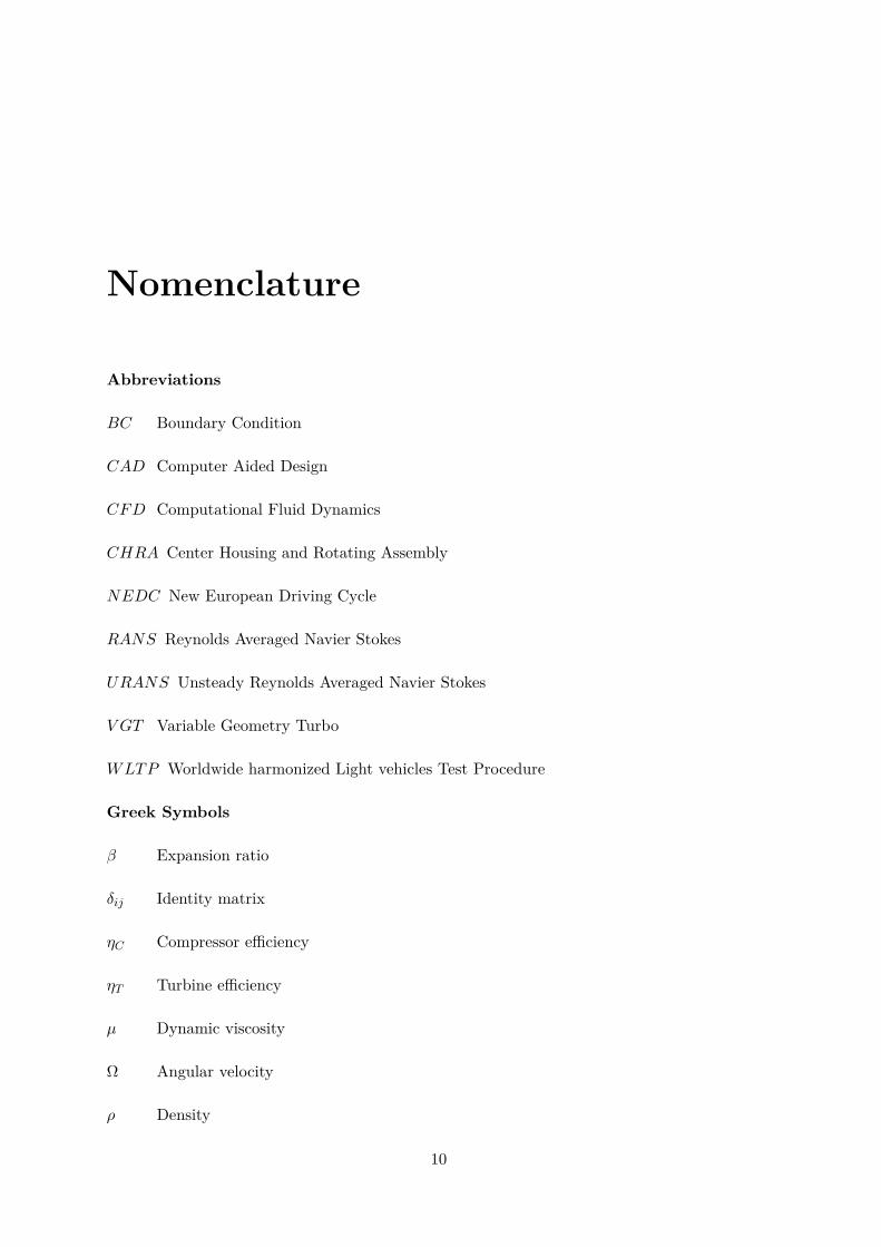
Abbreviations
BC Boundary Condition
CAD Computer Aided Design
CFD Computational Fluid Dynamics
CHRA Center Housing and Rotating Assembly
NEDC New European Driving Cycle
RANS Reynolds Averaged Navier Stokes
URANS Unsteady Reynolds Averaged Navier Stokes
V GT Variable Geometry Turbo
WLTP Worldwide harmonized Light vehicles Test Procedure
Greek Symbols
β Expansion ratio
δij Identity matrix
ηC Compressor efficiency
ηT Turbine efficiency
µ Dynamic viscosity
Ω Angular velocity
ρ Density
10
NOMENCLATURE
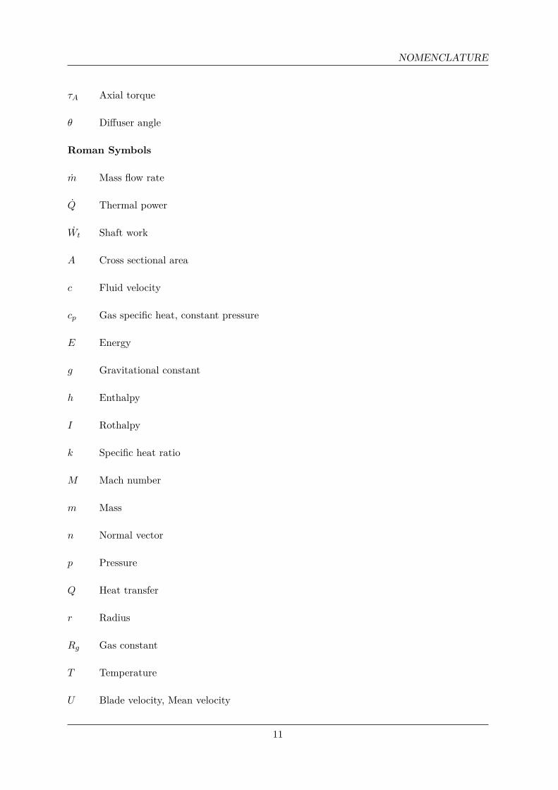
τA Axial torque
θ Diffuser angle
Roman Symbols
m Mass flow rate
Q Thermal power
Wt Shaft work
A Cross sectional area
c Fluid velocity
cp Gas specific heat, constant pressure
E Energy
g Gravitational constant
h Enthalpy
I Rothalpy
k Specific heat ratio
M Mach number
m Mass
n Normal vector
p Pressure
Q Heat transfer
r Radius
Rg Gas constant
T Temperature
U Blade velocity, Mean velocity
11
NOMENCLATURE
u Velocity
W Work
w Relative velocity
z Height
Subscripts
θ Tangential direction
i, j, k Direction
rel Relative property
0 Stagnation property, Volute inlet
1 Stator inlet
2 Stator throat
3 Stator outlet
4 Rotor inlet
5 Rotor throat
6 Rotor outlet
7 Diffuser outlet
12
Abstract
The current trend of vehicle manufacturers is increasingly driven towards the use of downsizing
technology, which coupled with turbocharging technique, allows to obtain engines with higher
power densities and characteristics in terms of emissions, performance and fuel consumption
much better than a conventional engine. The achievement of this target is clearly not any easy
task for developers which have to perform a considerable amount of studies to optimize the
system and find the compromise which best fits all requirements. Therefore, fluid dynamic
analysis, using dedicated CFD softwares, in addition to experimental tests, are fundamental
for the analysis and optimization of engine turbomatching: the former in particular becomes
essential considering the lack of data often available and the huge amount of time required at
the test bench.
The objective of the thesis was to develop a methodology that could be used for radial turbine
geometrical parameters optimization based on CFD analysis and its application to engine
performance assessment. Initially, 3D fluid dynamic studies will be performed on the model, in
order to evaluate the actual behaviour of the component, in terms of pressure and temperature
drop and gather useful data. Afterwards, collected information will be used to simulate the
response of the system using the overall model of the engine created through GT-Power in
a 0-dimensional approach, firstly evaluating the standard turbine and then rating the impact
that geometry changes on turbine design could have on overall engine performance.
Keywords: Turbocharger, turbomatching, turbine, CFD, GT-Power, SolidWorks, SolidWorks
Flow Simulation, geometrical turbine parameters, turbine characteristcs
13
Chapter 1
Introduction
1.1 Background
Nowadays more and more importance is placed on improving performance and emissions of
engines due to the global move to reduce CO2 emissions, where the target for 2021 is set to
< 95 [g/km], with further reduction of 15% and 37.5% expected respectively by 2025 and
2030. Car manufacturers has to strictly follow regulations to omologate new vehichles in
terms of pollutant emissions, following specific driving cycles, such as NEDC (New European
Driving Cycle) or WLTP (Worldwide Harmonized Light-Duty Vehicle Test Procedure) which
has become the new European standard.
Turbocharging technique is crucial to achieve and improve these aspects, mainly by enabling
engine’s downsizing (usage of a smaller engine capable to deliver the same power of a bigger
one). Moreover, one of the biggest source of inefficiency of the combustion process is the
significant amount of fuel energy wasted through the exhaust. Turbochargers recover some of
that energy to increase intake pressure, improving power density and efficiency. Therefore, it
is necessary to develop an optimum turbocharging system, to suit the engine requirements.
”Computational fluid dynamics or CFD is the analysis of systems involving fluid flow, heat
transfer and associated phenomena such as chemical reactions by means of computer-based
simulation” [1]. Fluid flow may be very hard to predict and differential equations that are
used in fluid mechanics are difficult to solve. Technological growth, understood both as the
development of powerful computers and numerical algorithms, gave the chance to solve these
kind of physical problems and has made it possible to use CFD as a research and design tool.
14
CHAPTER 1. INTRODUCTION
1.2 Turbocharger fundamentals
1.2.1 Working principle
Supercharging and turbocharging are the of the most common used methods of forced gases
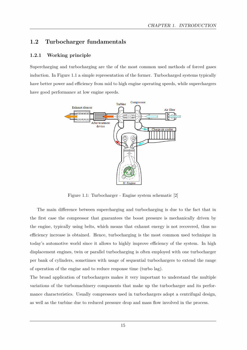
induction. In Figure 1.1 a simple representation of the former. Turbocharged systems typically
have better power and efficiency from mid to high engine operating speeds, while superchargers
have good performance at low engine speeds.
Figure 1.1: Turbocharger - Engine system schematic [2]
The main difference between supercharging and turbocharging is due to the fact that in
the first case the compressor that guarantees the boost pressure is mechanically driven by
the engine, typically using belts, which means that exhaust energy is not recovered, thus no
efficiency increase is obtained. Hence, turbocharging is the most common used technique in
today’s automotive world since it allows to highly improve efficiency of the system. In high
displacement engines, twin or parallel turbocharging is often employed with one turbocharger
per bank of cylinders, sometimes with usage of sequential turbochargers to extend the range
of operation of the engine and to reduce response time (turbo lag).
The broad application of turbochargers makes it very important to understand the multiple
variations of the turbomachinery components that make up the turbocharger and its perfor-
mance characteristics. Usually compressors used in turbochargers adopt a centrifugal design,
as well as the turbine due to reduced pressure drop and mass flow involved in the process.
15
CHAPTER 1. INTRODUCTION
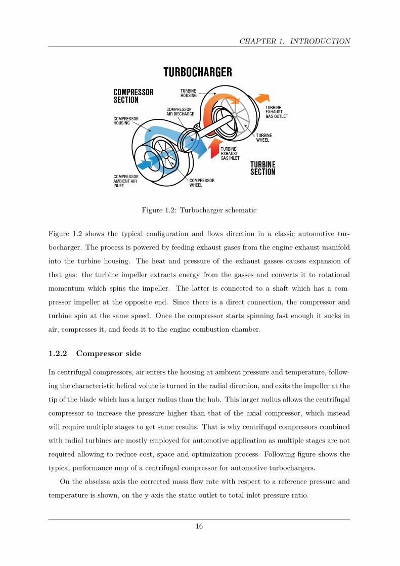
Figure 1.2: Turbocharger schematic
Figure 1.2 shows the typical configuration and flows direction in a classic automotive tur-
bocharger. The process is powered by feeding exhaust gases from the engine exhaust manifold
into the turbine housing. The heat and pressure of the exhaust gasses causes expansion of
that gas: the turbine impeller extracts energy from the gasses and converts it to rotational
momentum which spins the impeller. The latter is connected to a shaft which has a com-
pressor impeller at the opposite end. Since there is a direct connection, the compressor and
turbine spin at the same speed. Once the compressor starts spinning fast enough it sucks in
air, compresses it, and feeds it to the engine combustion chamber.
1.2.2 Compressor side
In centrifugal compressors, air enters the housing at ambient pressure and temperature, follow-
ing the characteristic helical volute is turned in the radial direction, and exits the impeller at the
tip of the blade which has a larger radius than the hub. This larger radius allows the centrifugal
compressor to increase the pressure higher than that of the axial compressor, which instead
will require multiple stages to get same results. That is why centrifugal compressors combined
with radial turbines are mostly employed for automotive application as multiple stages are not
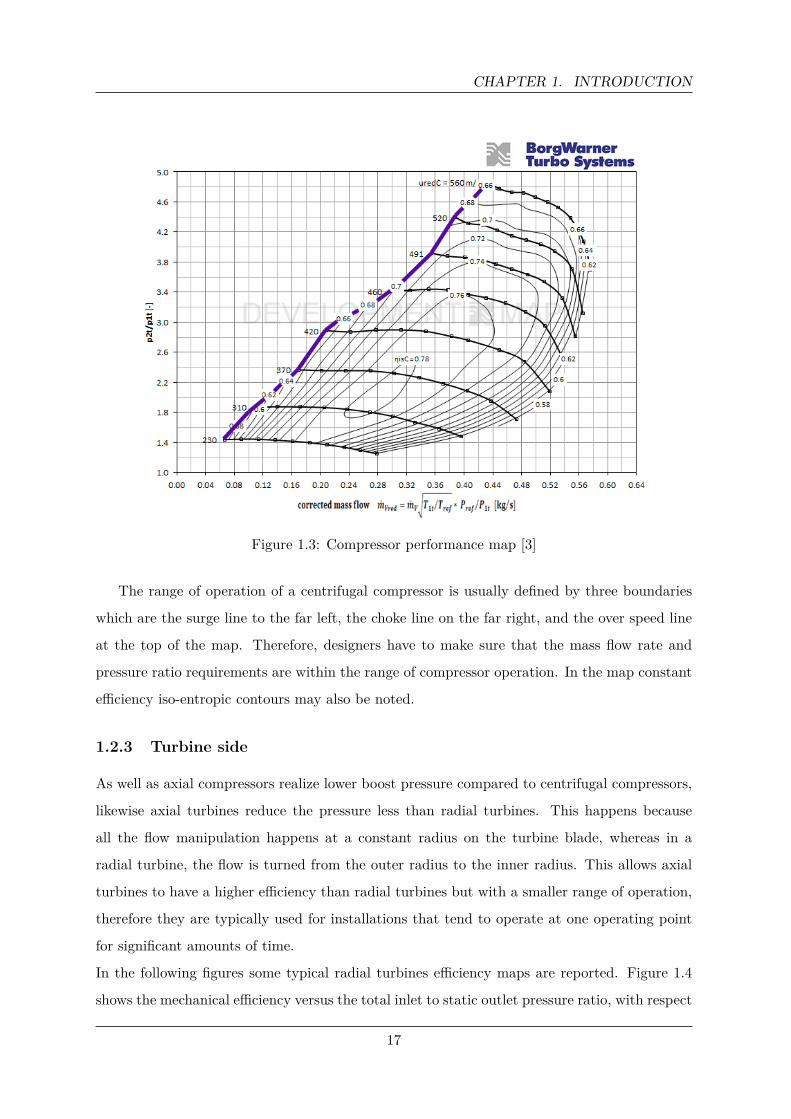
required allowing to reduce cost, space and optimization process. Following figure shows the
typical performance map of a centrifugal compressor for automotive turbochargers.
On the abscissa axis the corrected mass flow rate with respect to a reference pressure and
temperature is shown, on the y-axis the static outlet to total inlet pressure ratio.
16
CHAPTER 1. INTRODUCTION
Figure 1.3: Compressor performance map [3]
The range of operation of a centrifugal compressor is usually defined by three boundaries
which are the surge line to the far left, the choke line on the far right, and the over speed line
at the top of the map. Therefore, designers have to make sure that the mass flow rate and
pressure ratio requirements are within the range of compressor operation. In the map constant
efficiency iso-entropic contours may also be noted.
1.2.3 Turbine side
As well as axial compressors realize lower boost pressure compared to centrifugal compressors,
likewise axial turbines reduce the pressure less than radial turbines. This happens because
all the flow manipulation happens at a constant radius on the turbine blade, whereas in a
radial turbine, the flow is turned from the outer radius to the inner radius. This allows axial
turbines to have a higher efficiency than radial turbines but with a smaller range of operation,
therefore they are typically used for installations that tend to operate at one operating point
for significant amounts of time.
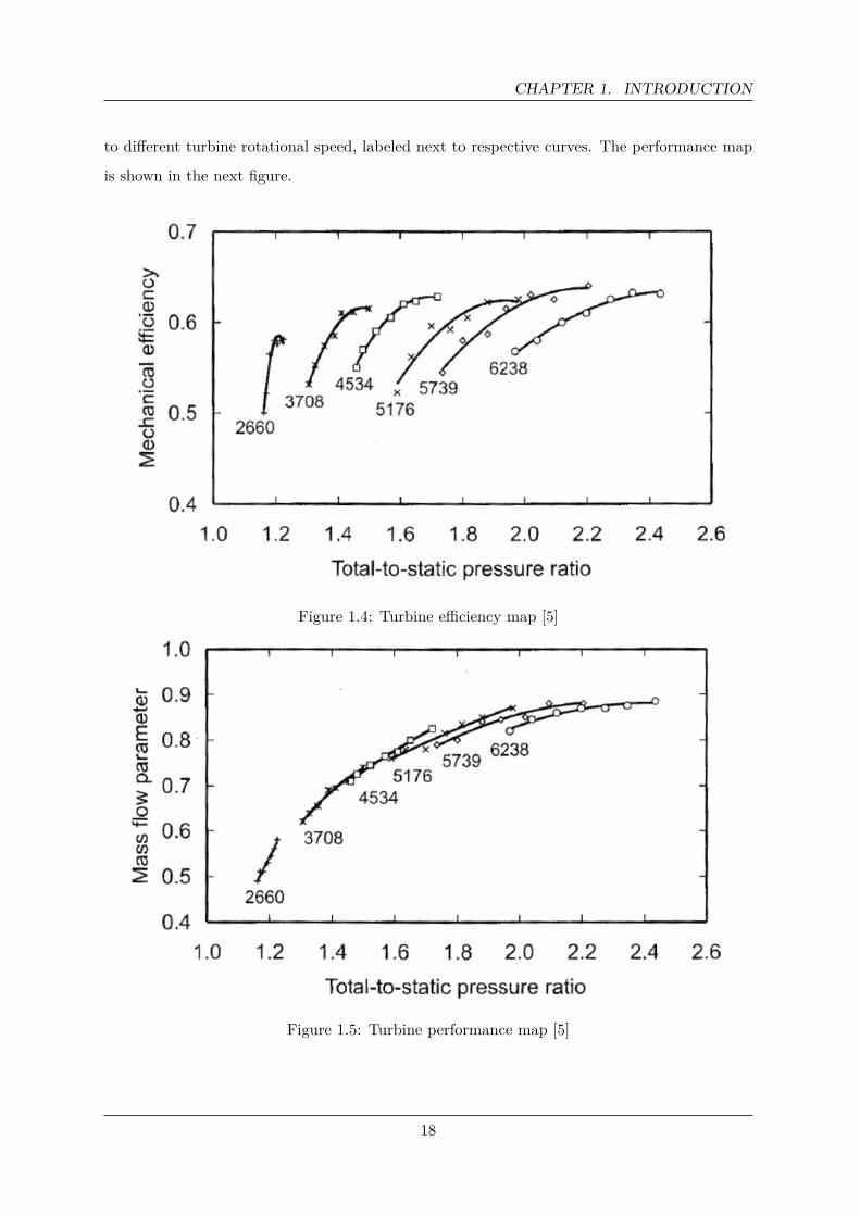
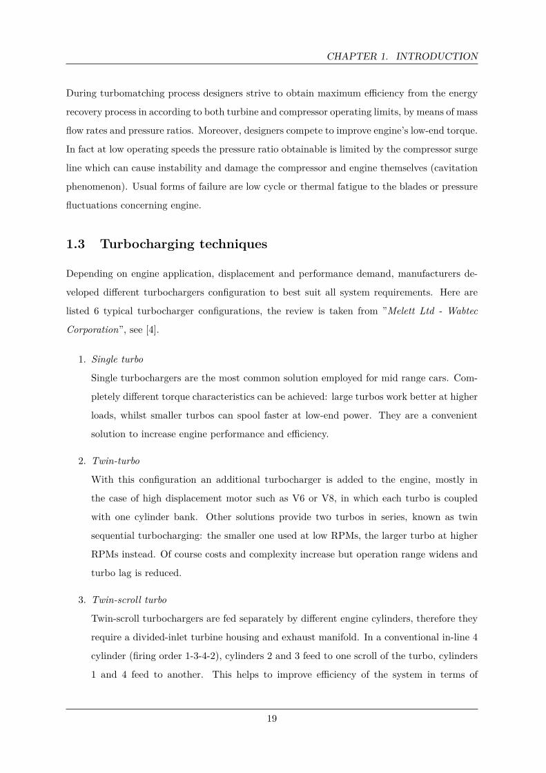
In the following figures some typical radial turbines efficiency maps are reported. Figure 1.4
shows the mechanical efficiency versus the total inlet to static outlet pressure ratio, with respect
17
CHAPTER 1. INTRODUCTION
to different turbine rotational speed, labeled next to respective curves. The performance map
is shown in the next figure.
Figure 1.4: Turbine efficiency map [5]
Figure 1.5: Turbine performance map [5]
18
CHAPTER 1. INTRODUCTION
During turbomatching process designers strive to obtain maximum efficiency from the energy
recovery process in according to both turbine and compressor operating limits, by means of mass
flow rates and pressure ratios. Moreover, designers compete to improve engine’s low-end torque.
In fact at low operating speeds the pressure ratio obtainable is limited by the compressor surge
line which can cause instability and damage the compressor and engine themselves (cavitation
phenomenon). Usual forms of failure are low cycle or thermal fatigue to the blades or pressure
fluctuations concerning engine.
1.3 Turbocharging techniques
Depending on engine application, displacement and performance demand, manufacturers de-
veloped different turbochargers configuration to best suit all system requirements. Here are
listed 6 typical turbocharger configurations, the review is taken from ”Melett Ltd - Wabtec
Corporation”, see [4].
1. Single turbo
Single turbochargers are the most common solution employed for mid range cars. Com-
pletely different torque characteristics can be achieved: large turbos work better at higher
loads, whilst smaller turbos can spool faster at low-end power. They are a convenient
solution to increase engine performance and efficiency.
2. Twin-turbo
With this configuration an additional turbocharger is added to the engine, mostly in
the case of high displacement motor such as V6 or V8, in which each turbo is coupled
with one cylinder bank. Other solutions provide two turbos in series, known as twin
sequential turbocharging: the smaller one used at low RPMs, the larger turbo at higher
RPMs instead. Of course costs and complexity increase but operation range widens and
turbo lag is reduced.
3. Twin-scroll turbo
Twin-scroll turbochargers are fed separately by different engine cylinders, therefore they
require a divided-inlet turbine housing and exhaust manifold. In a conventional in-line 4
cylinder (firing order 1-3-4-2), cylinders 2 and 3 feed to one scroll of the turbo, cylinders
1 and 4 feed to another. This helps to improve efficiency of the system in terms of
19
CHAPTER 1. INTRODUCTION
generated power and reduced turbo lag, but the main drawback is the cost associated
with the complexity of the turbine housing and the exhaust manifold.
4. Variable Geometry turbo
VGTs are one of the most common used solution amongst light commercial vehicles since
they allow to obtain, along with reduced costs higher performance than single turbo
layout. The turbine housing is made of a ring of aerodynamically-shaped vanes which
are controlled both via pneumatic or electronic components and enable to vary the cross-
sectional area of the turbine. The rack position allows to control the turbos area-to-radius
(A/R) ratio in order to give high low-end torque at low RPMs, and solid power at higher
revs. This results in reduced turbo lag and smoother torque band. Typically their usage
is limited to diesel engine car, since exhaust gases temperature in petrol car would be
much higher resulting in huge costs to realize vanes in particular heat resistant alloy.
5. Variable twin-scroll turbo
A VTS turbocharger combines the advantages of a twin-scroll turbo and a VGT. Using
a valve the system is able to redirect the flow just to one scroll or to both if the engine
requires it. The VTS turbocharger design provides a cheaper alternative to VGT turbos,
suitable for petrol engine applications.
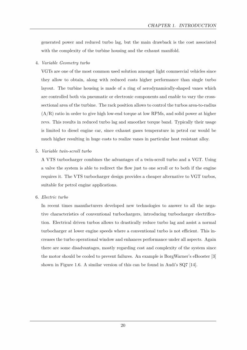
6. Electric turbo
In recent times manufacturers developed new technologies to answer to all the nega-
tive characteristics of conventional turbochargers, introducing turbocharger electrifica-
tion. Electrical driven turbos allows to drastically reduce turbo lag and assist a normal
turbocharger at lower engine speeds where a conventional turbo is not efficient. This in-
creases the turbo operational window and enhances performance under all aspects. Again
there are some disadvantages, mostly regarding cost and complexity of the system since
the motor should be cooled to prevent failures. An example is BorgWarner’s eBooster [3]
shown in Figure 1.6. A similar version of this can be found in Audi’s SQ7 [14].
20
CHAPTER 1. INTRODUCTION
Figure 1.6: BorgWarner’s eBooster scheme [3]
1.4 CFD analysis software
In the present study, CFD simulation on a radial turbocharger was conducted to analyze
the impact of geometry changes on the turbine stage, using different CFD software such as
SolidWorks Flow Simulation and GT-Power Suite.
The former was mainly used to carry out 3D CFD simulations to study the flow trend inside the
turbine scrolls, optimize internal aerodynamics and collect data about pressure and temperature
drops of the turbine volute, as well as the acceleration given to the fluid.
The latter enables to put the turbocharger inside a more complex environment, where the
whole engine could be simulated. This allows more in-depth investigation about the impact
of the different turbine A/R ratio over the engine performance, BSFC and efficiency, giving a
wide panorama of the different working conditions.
21
CHAPTER 1. INTRODUCTION
1.4.1 SOLIDWORKS FloXpressTM
The package FloXpress is a preliminary data flow analysis tool in which water or air concen-
trates on parts or assemblies. After defining input and boundary conditions for the model, the
software roughly calculates flow trajectories, showing in particular flow’s velocity. Thanks to
that, it’s possible to find any issues in the project and improve them before building the actual
parts [8].
1.4.2 SOLIDWORKS Flow SimulationTM
Flow Simulation is the next step in fluid dynamic analysis. It is a general-purpose fluid flow and
heat transfer simulation tool capable of simulating both low-speed and supersonic flows. The
advantages compared to the other package are considerable. Besides allowing a better control of
the geometry to evaluate the correct flow path, this tool allows to define with greater accuracy
the parameters of the analysis, in order to obtain very high quality results and adherent to
the reality [8]. This paper takes advantage of some of them in particular, e.g the possibility of
defining a rotating mesh to simulate the rotation of the impeller or the ability to define custom
fluids to perform calculations, exhaust gases in this specific case.
1.4.3 GT-POWER SuiteTM
GT-POWER is the industry standard engine performance simulation, used to predict engine
performance quantities such as power, torque, airflow, volumetric efficiency, fuel consump-
tion, turbocharger performance and matching, and pumping losses. Beyond basic performance
predictions, GT-POWER includes physical models for extending the predictions to include
cylinder and tailpipe-out emissions, intake and exhaust system acoustic characteristics (level
and quality), in-cylinder and pipe/manifold structure temperature, measured cylinder pressure
analysis, and control system modeling [9].
22
Chapter 2
Literature review
The turbocharger is made up of different components: the compressor, the turbine, main
housing and the shaft. The rotor of the turbocharger is supported by a bearing system which
has to stand critical conditions, assuming revolution speeds up to 150k rpm. Both the turbine
and compressor impellers are linked to rotating shaft, resulting in the same rotational speed.
A fundamental understanding of the flow behavior of a radial turbine is necessary to be
able to properly read the results from the CFD calculation performed in this simulation.
2.1 Radial turbine theory
The design of a radial turbine can be represented by the turbine housing, the rotor and the
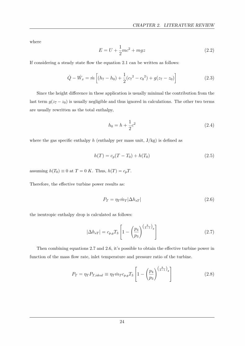
stator. The thermodynamic process which evolve inside the component is shown in the h-s
diagram of Figure 2.1 an h-s. Each point is indicative for the area that the fluid is going
through at that specific moment. 0 label stands for volute inlet, 1 for nozzle inlet, 2 stator
throat, 3 stator outlet, 4 rotor inlet, 5 rotor throat, 6 rotor outlet and 7 diffuser outlet. The
energy recovery process, thus the mechanical power output is obtained at the rotor stage,
thanks to the heat and the pressure drop granted by expanding exhaust gases. The amount of
power extracted depends on the mass flow rate of the exhaust gas, the expansion ratio and the
isentropic enthalpy drop in the turbine itself.
2.1.1 Governing equations
Writing the First Law of Thermodynamics for an for an infinitesimal variation of state [6]:
dE = dQ− dWt (2.1)
23
CHAPTER 2. LITERATURE REVIEW
where
E = U + 12mc
2 +mgz (2.2)
If considering a steady state flow the equation 2.1 can be written as follows:
Q− Wx = m[(h7 − h0) + 1
2(c72 − c0
2) + g(z7 − z0)]
(2.3)
Since the height difference in these application is usually minimal the contribution from the
last term g(z7− z0) is usually negligible and thus ignored in calculations. The other two terms
are usually rewritten as the total enthalpy,
h0 = h+ 12c
2 (2.4)
where the gas specific enthalpy h (enthalpy per mass unit, J/kg) is defined as
h(T ) = cp(T − T0) + h(T0) (2.5)
assuming h(T0) ≡ 0 at T = 0 K. Thus, h(T ) = cpT .
Therefore, the effective turbine power results as:
PT = ηT mT |∆hsT | (2.6)
the isentropic enthalpy drop is calculated as follows:
|∆hsT | = cp,gT3
1−(p4
p3
)( kk−1)
g
(2.7)
Then combining equations 2.7 and 2.6, it’s possible to obtain the effective turbine power in
function of the mass flow rate, inlet temperature and pressure ratio of the turbine.
PT = ηTPT,ideal ≡ ηT mT cp,gT3
1−(p4
p3
)( kk−1)
g
(2.8)
24
CHAPTER 2. LITERATURE REVIEW
Figure 2.1: h-s diagram of the process of a radial turbine [7]
25
CHAPTER 2. LITERATURE REVIEW
Since the support bearing system is not ideal, it causes losses due to the friction and the
mechanical efficiency ηm must be considered to evaluate the absorbed power from compressor.
PT = ηmηTPT,ideal = ηmηT mT cp,gT3
1−(p4
p3
)( kk−1)
g
(2.9)
Likewise, it is possible to get compressor power from the isentropic drop and efficiency as
follows:
PC = PC,idealηC
≡ mC∆hsCηC
(2.10)
Using thermodynamic equations for an isentropic process, the required compressor power is
calculated:
PC = mCcp,aT1
ηC
(p2
p1
)( kk−1)
a
− 1 (2.11)
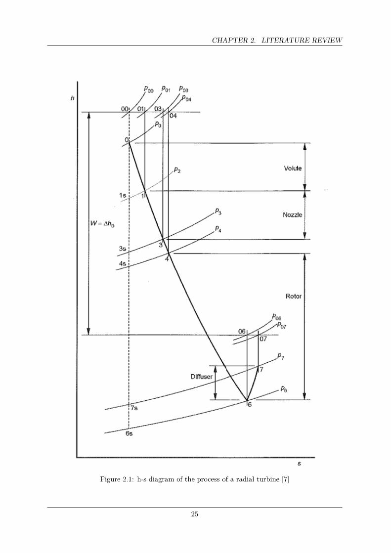
The performance map of the turbine shown in Figure 2.2 displays the corrected mass flow rate
over the turbine expansion ratio πT . Over a certain pressure ratio the mass flow rate is no
longer increasing which means that the flow is choked, even at higher rotational speeds. The
exhaust gas speed reaches the sonic speed with Mach number M = 1.
_mT ¼ lATp3t
ffiffiffiffiffiffiffiffiffiffiffi2
RgT3t
s ffiffiffiffiffiffiffiffiffiffiffiffiffiffiffiffiffiffiffiffiffiffiffiffiffiffiffiffiffiffiffiffiffiffiffiffiffiffiffiffiffiffiffiffiffiffiffiffiffiffiffiffiffiffiffiffiffiffiffiffiffiffiffiffiffiffiffiffiffiffij
j 1
g
p3tp4
2jg p3t
p4
jþ1jð Þg
!vuut ð2:17Þ
where µ is the flow coefficient due friction and flow contraction at the nozzle outlet,AT is the throttle cross-sectional area in the turbine wheel.
To eliminate the influences of p3t and T3t on the mass flow rate in the turbineshown in Eq. (2.17), the so-called corrected mass flow rate is defined as
_mT ;cor _mTffiffiffiffiffiffiT3t
pp3t
¼ f ðpT ;tsÞ
¼ lAT
ffiffiffiffiffi2Rg
s ffiffiffiffiffiffiffiffiffiffiffiffiffiffiffiffiffiffiffiffiffiffiffiffiffiffiffiffiffiffiffiffiffiffiffiffiffiffiffiffiffiffiffiffiffiffiffiffiffiffiffiffiffiffiffiffiffiffiffiffiffiffiffiffiffiffiffiffiffiffij
j 1
g
p3tp4
2jg p3t
p4
jþ1jð Þg
!vuut ð2:18Þ
Equation (2.18) indicates that the corrected mass flow rate of the turbine is inde-pendent of the inlet condition of the exhaust gas of p3t and T3t. It depends only onthe turbine expansion ratio πT,ts.
The performance map of the turbine displays the corrected mass flow rate overthe turbine expansion ratio πT,ts at various rotor speeds in Fig. 2.4. From a turbinepressure ratio of approximately 3, the mass flow rate has no longer increased, evenat higher rotor speeds. In this case, the flow in the turbine becomes a choked flow inwhich the exhaust gas speed at the throttle area reaches the sonic speed with Machnumber M = 1. As a result, the exhaust gas mass flow rate through the turbinecorresponding to the nominal engine power must be smaller than the mass flow rate
4
3
p
p tT ≡π
corTm ,
1.00
3.0
chokeTm ,
N1
N2
Nmax
Fig. 2.4 Performance map of the turbine
2.3 Turbocharger Equations 27
Figure 2.2: Turbine performance map [6]
26
CHAPTER 2. LITERATURE REVIEW
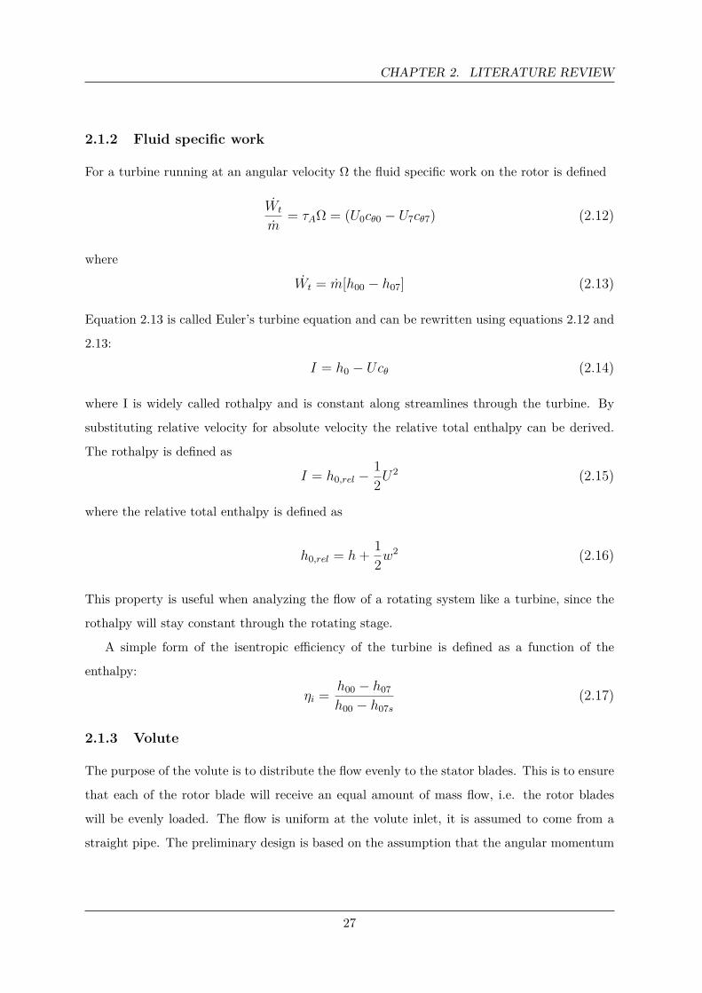
2.1.2 Fluid specific work
For a turbine running at an angular velocity Ω the fluid specific work on the rotor is defined
Wt
m= τAΩ = (U0cθ0 − U7cθ7) (2.12)
where
Wt = m[h00 − h07] (2.13)
Equation 2.13 is called Euler’s turbine equation and can be rewritten using equations 2.12 and
2.13:
I = h0 − Ucθ (2.14)
where I is widely called rothalpy and is constant along streamlines through the turbine. By
substituting relative velocity for absolute velocity the relative total enthalpy can be derived.
The rothalpy is defined as
I = h0,rel −12U
2 (2.15)
where the relative total enthalpy is defined as
h0,rel = h+ 12w
2 (2.16)
This property is useful when analyzing the flow of a rotating system like a turbine, since the
rothalpy will stay constant through the rotating stage.
A simple form of the isentropic efficiency of the turbine is defined as a function of the
enthalpy:
ηi = h00 − h07
h00 − h07s(2.17)
2.1.3 Volute
The purpose of the volute is to distribute the flow evenly to the stator blades. This is to ensure
that each of the rotor blade will receive an equal amount of mass flow, i.e. the rotor blades
will be evenly loaded. The flow is uniform at the volute inlet, it is assumed to come from a
straight pipe. The preliminary design is based on the assumption that the angular momentum
27
CHAPTER 2. LITERATURE REVIEW
is constant, described by the free vortex equation and the continuity equation in θ direction:
rCθ = const
mθ = ρθAθCθ
(2.18)
2.2 Solidworks - Computational architecture
The realization of a CFD analysis requires an accurate phase of process structuring. In fact,
the results obtainable are variable depending on the validity of the models used, as well as on
the robustness of the calculation methods implemented within the software. Therefore it is
essential to find an optimal solution which, at the same time, guarantees reduced simulation
times but a suitable accuracy for that specific task. Different equations could be used such
as Reynolds Averaged Navier Stokes (RANS) for steady simulation and Unsteady Reynolds
Averaged Navier Stokes (URANS) for transient.
2.2.1 Governing equations
Flow Simulation solves the Navier-Stokes equations, which are formulations of mass, momentum
and energy conservation laws for fluid flows. The equations are correlated by state equations
defining the type of the fluid, and by empirical dependencies of density, and thermal conductiv-
ity. A particular problem is specified from the user by the definition of its geometry, shape and
initial value conditions. The conservation laws for mass, angular momentum and energy in the
Cartesian coordinate system rotating with angular velocity Ω about an axis passing through
the coordinate system’s origin can be written in the conservation form as follows [8]:
∂ρ
∂t+ ∂
∂xi(ρui) = 0 (2.19)
∂(ρui)∂t
+ ∂
∂xj(ρuiuj) + ∂p
∂xi= ∂
∂xj(τij + τRij ) + Si i = 1, 2, 3 (2.20)
∂ρH
∂t+ ∂ρuiH
∂xj= ∂
∂xi
(uj(τij + τRij ) + qi
)+ ∂p
∂t− τRij
∂ui∂xj
+ ρε+ Siui +QH (2.21)
where u is the fluid velocity, ρ is the fluid density, Si is a mass-distributed external force per
unit mass due to a porous media resistance, a buoyancy and the coordinate system’s rotation,
28
CHAPTER 2. LITERATURE REVIEW
i.e., Si = Sporousi +Sgravityi +Srotationi , h is the thermal enthalpy, QH is a heat source or sink per
unit volume, τik is the viscous shear stress tensor, qi is the diffusive heat flux. The subscripts
are used to denote summation over the tree coordinate directions. For Newtonian fluids the
viscous shear stress tensor is defined as:
τij = µ
(∂ui∂xj
+ ∂uj∂xi− 2
3δij∂uk∂xk
)(2.22)
Here δij is the Kronecker delta function (it is equal to unity when i = j, and zero otherwise),
and µ is the dynamic viscosity coefficient.
2.2.2 Laminar/turbulent boundary model
This type of model is typically used to define flows in near-wall regions. The model is based
on the so-called Modified Wall Functions approach. This enables to characterize laminar and
turbulent flows near the walls, and to describe flows transitions from one type to the other,
using the Van Driest’s profile instead of a logarithmic profile. If the size of the mesh cell near
the wall is more than the boundary layer thickness the integral boundary layer technology is
used. The model provides efficient profiles of temperature and velocity for the above mentioned
conservation equations [8].
2.2.3 Mesh
”Flow Simulation computational approach is based on locally refined rectangular mesh near
geometry boundaries. The mesh cells are rectangular parallelepipeds with faces orthogonal
to the specified axes of the Cartesian coordinate system. However, near the boundary mesh
cells are more complex. The near-boundary cells are portions of the original parallelepiped
cells that cut by the geometry boundary. The curved geometry surface is approximated by
set of polygons which vertexes are surface’s intersection points with the cells’ edges. These
flat polygons cut the original parallelepiped cells. Thus, the resulting near-boundary cells are
polyhedrons with both axis-oriented and arbitrary oriented plane faces in this case. The original
parallelepiped cells containing boundary are split into several control volumes that are referred
to only one fluid or solid medium. In the simplest case there are only two control volumes in
the parallelepiped, one is solid and another is fluid” [8].
The rectangular computational domain is automatically constructed (may be changed manu-
ally), so it encloses the solid body and has the boundary planes orthogonal to the specified
29
CHAPTER 2. LITERATURE REVIEW
Flow Simulation 2017 Technical Reference 67
The rectangular computational domain is automatically constructed (may be changed manually), so it encloses the solid body and has the boundary planes orthogonal to the specified axes of the Cartesian coordinate system. Then, the computational mesh is constructed in the following several stages.
First of all, a basic mesh is constructed. For that, the computational domain is divided into slices by the basic mesh planes, which are evidently orthogonal to the axes of the Cartesian coordinate system. The user can specify the number and spacing of these planes along each of the axes. The so-called control planes whose position is specified by user can be among these planes also. The basic mesh is determined solely by the computational domain and does not depend on the solid/fluid interfaces.
Fig.4.1Computational mesh near the solid/fluid interface.
centers of fluid control volumes
centers of solid control volumes
original curved geometry boundary
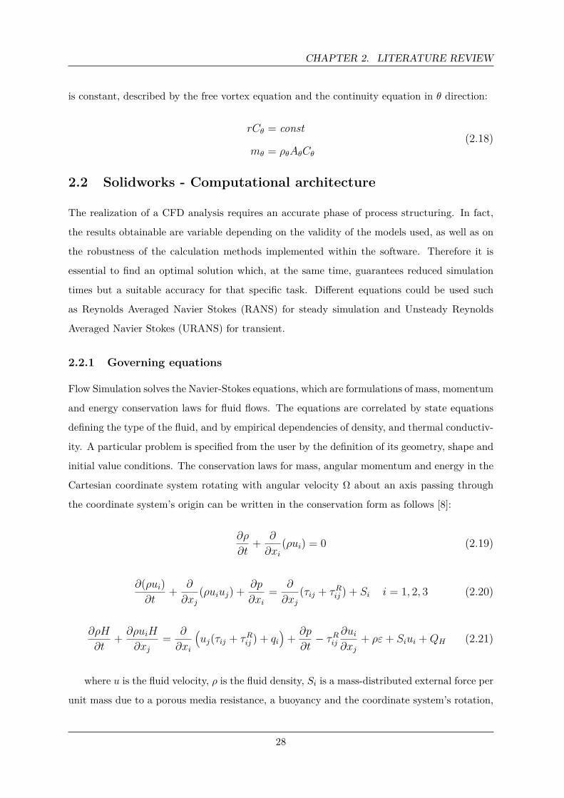
Figure 2.3: Computational mesh near the solid/fluid interface [8]
axes of the Cartesian coordinate system. Then, the computational mesh is built.
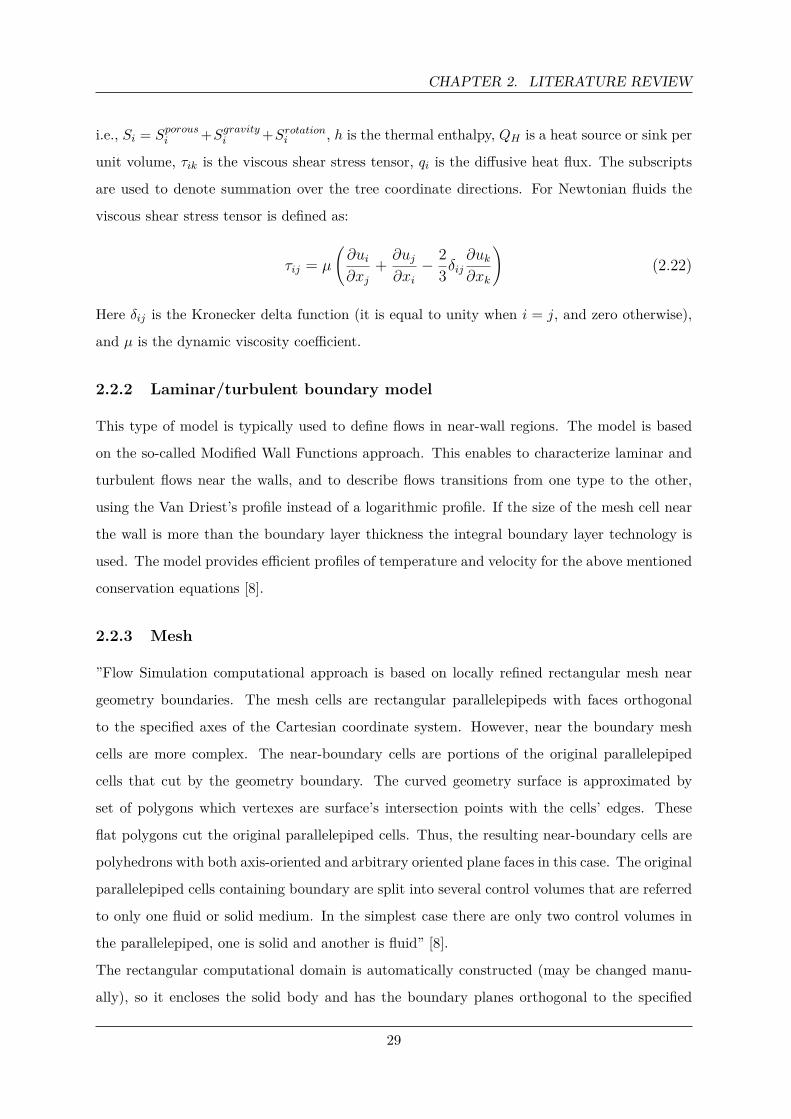
In Figure 2.4 and Table 2.1 the quality criteria for the solver is specified. The figure shows
how the angle for the quadrilateral faced element is not as good as it could be. The normal
vector for the integration point surface, n, and the vector that joins two control volume nodes,
s, are not parallel. However for the triangular faced element the orthogonality is of highest
order since the vectors are parallel. The best measurement on the mesh orthogonality is the
orthogonality angle which is the area weighted average of 90− acos(n · s). According to Table
2.1 the area weighted average of the orthogonality angle can not be smaller than 20 but local
angles can be as low as 10.
Here are described some of the criteria that the software uses to generate the mesh.
30
CHAPTER 2. LITERATURE REVIEW
Figure 2.4: Orthogonality for quadrilateral and triangular faced elements
Measure Acceptable range Description
Orthogonality factor >20Area weighted average of 90 -
acos(n · s)
Orthogonality minimum angle 1/3 Area weighted average n · s
Orthogonality factor >10 Minimum of n · s
Minimum and maximum face angle >10 and <170Minimum and maximum angle
between edges of each face
Minimum and maximum dihedral angle >10 and <170Minimum and maximum angle
between element face
Table 2.1: Solidworks Flow Simulation mesh criteria
2.3 GT-Power model implementation
Turbine and compressor performance are modeled in the software using performance maps
which can be summarized as a series of performance data points, each of which describes the
operating condition by speed, pressure ratio, mass flow rate, and thermodynamic efficiency.
The maps are configured so that if the speed and either the mass flow or pressure ratio are
known, the efficiency and either the mass flow rate or pressure ratio can be found in the map.
The software predicts the turbocharger speed and the pressure ratio (PR) across turbine and/or
compressor at each timestep, and therefore they are ”known” with respect to the turbo map.
The mass flow rate and efficiency are then looked up in the table and imposed in the solution.
31
CHAPTER 2. LITERATURE REVIEW
2.3.1 Maps evaluation
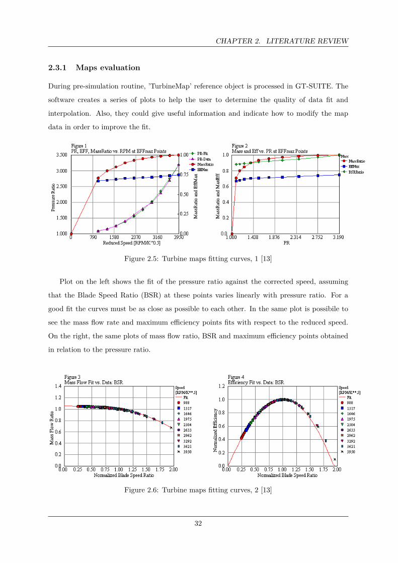
During pre-simulation routine, ’TurbineMap’ reference object is processed in GT-SUITE. The
software creates a series of plots to help the user to determine the quality of data fit and
interpolation. Also, they could give useful information and indicate how to modify the map
data in order to improve the fit.
CHAPTER 3
72 Gamma Technologies, Inc. © 2014
3.6 Evaluation and Modification of Turbine Maps There are two aspects that are critical to modeling engines with turbines: obtaining good data, and obtaining a good fit to that data for extrapolation to points outside of the data range. The turbine map fitting method in GT-POWER depends upon the true maximum efficiency of a speed or pressure ratio line being present in the data. Please read the section on the turbine map fitting method for more details. When the true maximum efficiency is not present in a speed line or is unclear due to noisy data, the quality of the fit will decrease. The extent to which it decreases will depend upon how much difference exists between the pressure ratio of the maximum efficiency found in the data versus the pressure ratio of the true maximum efficiency for that speed line.
3.6.1 Examination of the Messages in the *.out File While GT-POWER is pre-processing the maps, it is also checking the data for problems. Any problem that is found is reported on the run screen during pre-processing and also written to the *.out file. For example, a warning will be written for all speed lines for which the maximum efficiency is unclear. This is one of the most common causes of a problem with the fitting of turbine maps.
3.6.2 Evaluation of Turbine Maps When 'TurbineMap' and 'TurbineMapSAE' reference objects are processed in GT-SUITE, eight plots are produced which aid the user in determining the quality of the data, fit, and extrapolation. These plots can be used to evaluate the data and the quality of the fit. If needed, they can indicate how to modify the map data in order to improve the fit. The first page of four plots shows a mixture of both data quality and fit quality. Each of the following figures will be described. Following the description will be a discussion about which features of each plot are desirable and which features are undesirable. The first set of eight plots below shows how an ideal set of data appears.
Figure 1 shows plots of several curves that are used in the fitting procedure. The actual data and the fit of PR vs. RPM at the maximum efficiency point of each speed line are plotted. The fit is obtained by assuming that the Blade Speed Ratio (BSR) at these points varies linearly with pressure ratio (PR). (The BSR is defined in the next section, Turbine Fitting Method.) The two curves should be close to each other for a good fit. Figure 1 also shows the efficiency and normalized mass flow (MassRatio) for the maximum efficiency points versus speed. The MassRatio is mass flow rate at the maximum efficiency of the speed lines normalized by the largest mass flow rate of all the maximum efficiency points. The MassRatio should be linear near a speed of zero. The MassRatio should be smooth, with only one local maximum at a high speed.
Figure 2.5: Turbine maps fitting curves, 1 [13]
Plot on the left shows the fit of the pressure ratio against the corrected speed, assuming
that the Blade Speed Ratio (BSR) at these points varies linearly with pressure ratio. For a
good fit the curves must be as close as possible to each other. In the same plot is possibile to
see the mass flow rate and maximum efficiency points fits with respect to the reduced speed.
On the right, the same plots of mass flow ratio, BSR and maximum efficiency points obtained
in relation to the pressure ratio.
CHAPTER 3
73 Gamma Technologies, Inc. © 2014
Figure 2 shows the normalized mass flow rate and efficiency for the maximum efficiency points versus pressure ratio. It also shows the normalized BSR at maximum efficiency. (The BSR is normalized by the largest BSR of all of the maximum efficiency points.)
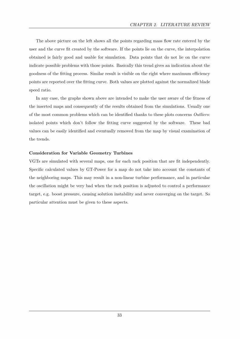
Figure 3 shows a plot of Mass Flow Ratio vs. BSR. It includes all of the data points entered by the user, on top of the curve fit. This plot gives the user an indication of the reliability of the fit. Data points that do not lie on the fit line indicate possible problems with those points. It also shows the range of the data with respect to BSR, compared to the whole range over which it has to be extrapolated. Measurements that include a wider range of BSR will provide a better fit and reduce the need for extrapolation. Figure 4 shows a plot of Efficiency vs. BSR. It includes the data points with the fitted curve. This plot gives the user an indication of the reliability of the fit. It also shows the range of input data with respect to BSR, compared to the whole range over which it has to be extrapolated.
Figure 5 shows the plot of the mass flow input data (up to 10 lines) compared to the fit curves evaluated for the same speed lines. These fits should be reviewed, and can be improved by entering the value of Mass Flow Ratio at 0 BSR or by entering data into the Max. Eff. Curve folder. (See the section Turbine Fitting Method for all fitting options.) The attribute Mass Flow Ratio at 0 BSR is found in the Shape folder of 'TurbineMap' and 'TurbineMapSAE'. Figure 6 shows the plot of the efficiency input data (up to 10 lines) compared to the map evaluated for the same speed lines. The quality of the map should be reviewed, and if needed can be improved by entering the values of Eff. Shape factor at Low BSR and Eff. Intercept at High BSR or by entering data into the Max. Eff. Curve folder. The attributes Eff. Shape factor at Low BSR and Eff. Intercept at High BSR are found in the Shape folder of 'TurbineMap' and 'TurbineMapSAE'.
Figure 2.6: Turbine maps fitting curves, 2 [13]
32
CHAPTER 2. LITERATURE REVIEW
The above picture on the left shows all the points regarding mass flow rate entered by the
user and the curve fit created by the software. If the points lie on the curve, the interpolation
obtained is fairly good and usable for simulation. Data points that do not lie on the curve
indicate possible problems with those points. Basically this trend gives an indication about the
goodness of the fitting process. Similar result is visible on the right where maximum efficiency
points are reported over the fitting curve. Both values are plotted against the normalized blade
speed ratio.
In any case, the graphs shown above are intended to make the user aware of the fitness of
the inserted maps and consequently of the results obtained from the simulations. Usually one
of the most common problems which can be identified thanks to these plots concerns Outliers:
isolated points which don’t follow the fitting curve suggested by the software. These bad
values can be easily identified and eventually removed from the map by visual examination of
the trends.
Consideration for Variable Geometry Turbines
VGTs are simulated with several maps, one for each rack position that are fit independently.
Specific calculated values by GT-Power for a map do not take into account the constants of
the neighboring maps. This may result in a non-linear turbine performance, and in particular
the oscillation might be very bad when the rack position is adjusted to control a performance
target, e.g. boost pressure, causing solution instability and never converging on the target. So
particular attention must be given to these aspects.
33
Chapter 3
Model description
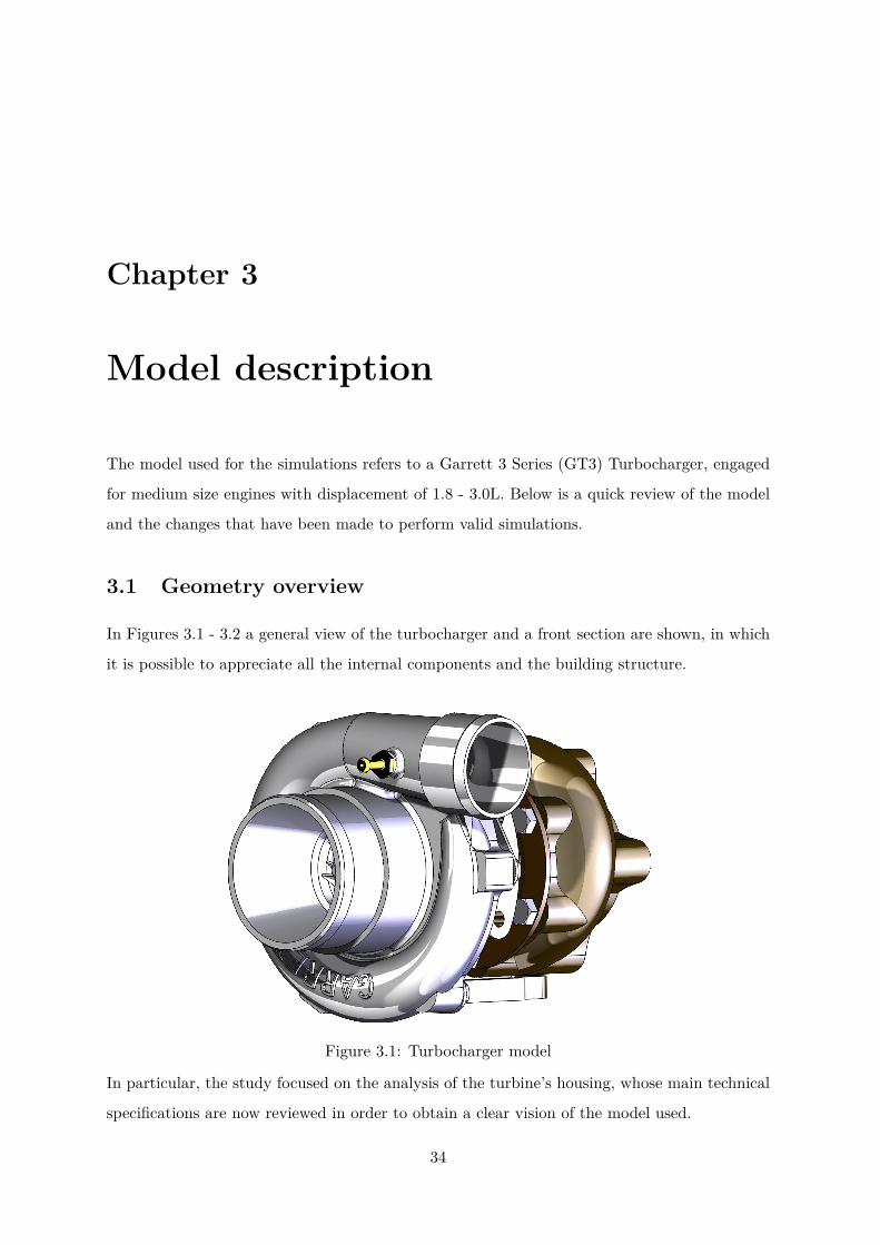
The model used for the simulations refers to a Garrett 3 Series (GT3) Turbocharger, engaged
for medium size engines with displacement of 1.8 - 3.0L. Below is a quick review of the model
and the changes that have been made to perform valid simulations.
3.1 Geometry overview
In Figures 3.1 - 3.2 a general view of the turbocharger and a front section are shown, in which
it is possible to appreciate all the internal components and the building structure.
Figure 3.1: Turbocharger model
In particular, the study focused on the analysis of the turbine’s housing, whose main technical
specifications are now reviewed in order to obtain a clear vision of the model used.
34
CHAPTER 3. MODEL DESCRIPTION
Figure 3.2: Turbocharger front section
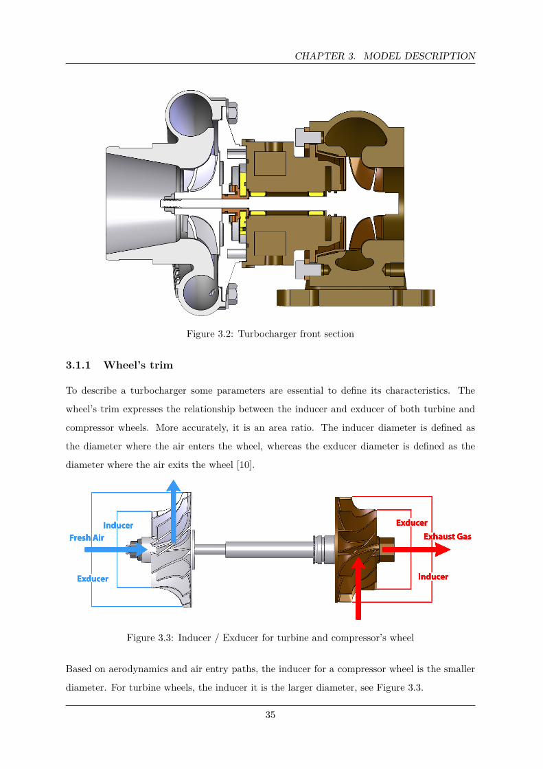
3.1.1 Wheel’s trim
To describe a turbocharger some parameters are essential to define its characteristics. The
wheel’s trim expresses the relationship between the inducer and exducer of both turbine and
compressor wheels. More accurately, it is an area ratio. The inducer diameter is defined as
the diameter where the air enters the wheel, whereas the exducer diameter is defined as the
diameter where the air exits the wheel [10].
InducerFresh Air
Exducer Inducer
Exducer
Exhaust Gas
Figure 3.3: Inducer / Exducer for turbine and compressor’s wheel
Based on aerodynamics and air entry paths, the inducer for a compressor wheel is the smaller
diameter. For turbine wheels, the inducer it is the larger diameter, see Figure 3.3.
35
CHAPTER 3. MODEL DESCRIPTION
Wheel’s trim, can be calculated in the following way, (measurements in calculations are
expressed in mm):
Trim =(
Inducer2
Exducer2
)· 100 (3.1)
Compressor’s trim
Trim,C =(
472
702
)· 100 = 45 (3.2)
Turbine’s trim
Trim,T =(
522
602
)· 100 = 75 (3.3)
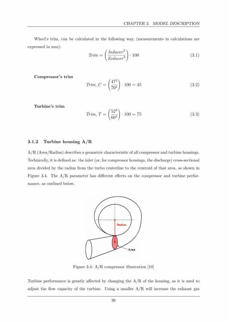
3.1.2 Turbine housing A/R
A/R (Area/Radius) describes a geometric characteristic of all compressor and turbine housings.
Technically, it is defined as: the inlet (or, for compressor housings, the discharge) cross-sectional
area divided by the radius from the turbo centerline to the centroid of that area, as shown in
Figure 3.4. The A/R parameter has different effects on the compressor and turbine perfor-
mance, as outlined below.
Figure 3.4: A/R compressor illustration [10]
Turbine performance is greatly affected by changing the A/R of the housing, as it is used to
adjust the flow capacity of the turbine. Using a smaller A/R will increase the exhaust gas
36
CHAPTER 3. MODEL DESCRIPTION
velocity into the turbine wheel. This provides increased turbine power at lower engine speeds,
resulting in a quicker boost rise. However, a small A/R also causes the flow to enter the
wheel more tangentially, which reduces the ultimate flow capacity of the turbine wheel, which
will tend to increase exhaust backpressure and hence reduce the engine’s ability to ”breathe”
effectively at high RPM, adversely affecting peak engine power.
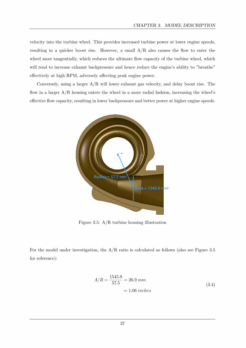
Conversely, using a larger A/R will lower exhaust gas velocity, and delay boost rise. The
flow in a larger A/R housing enters the wheel in a more radial fashion, increasing the wheel’s
effective flow capacity, resulting in lower backpressure and better power at higher engine speeds.
Figure 3.5: A/R turbine housing illustration
For the model under investigation, the A/R ratio is calculated as follows (also see Figure 3.5
for reference):
A/R = 1545.957.5 = 26.9 mm
= 1.06 inches(3.4)
37
CHAPTER 3. MODEL DESCRIPTION
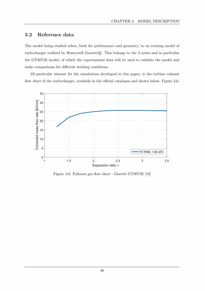
3.2 Reference data
The model being studied refers, both for performance and geometry, to an existing model of
turbocharger realized by Honeywell Garnett R©. This belongs to the 3 series and in particular
the GT3071R model, of which the experimental data will be used to validate the model and
make comparisons for different working conditions.
Of particular interest for the simulations developed in this paper, is the turbine exhaust
flow chart of the turbocharger, available in the official catalogue and shown below, Figure 3.6.
1 1.5 2 2.5 3 3.5Expansion ratio
0
5
10
15
20
25
30
35
Cor
rect
ed m
ass
flow
rate
[lb/
min
]
75 TRIM, 1.06 A/R
Figure 3.6: Exhaust gas flow chart - Garrett GT3071R [10]
38
Chapter 4
SolidWorks simulation setup
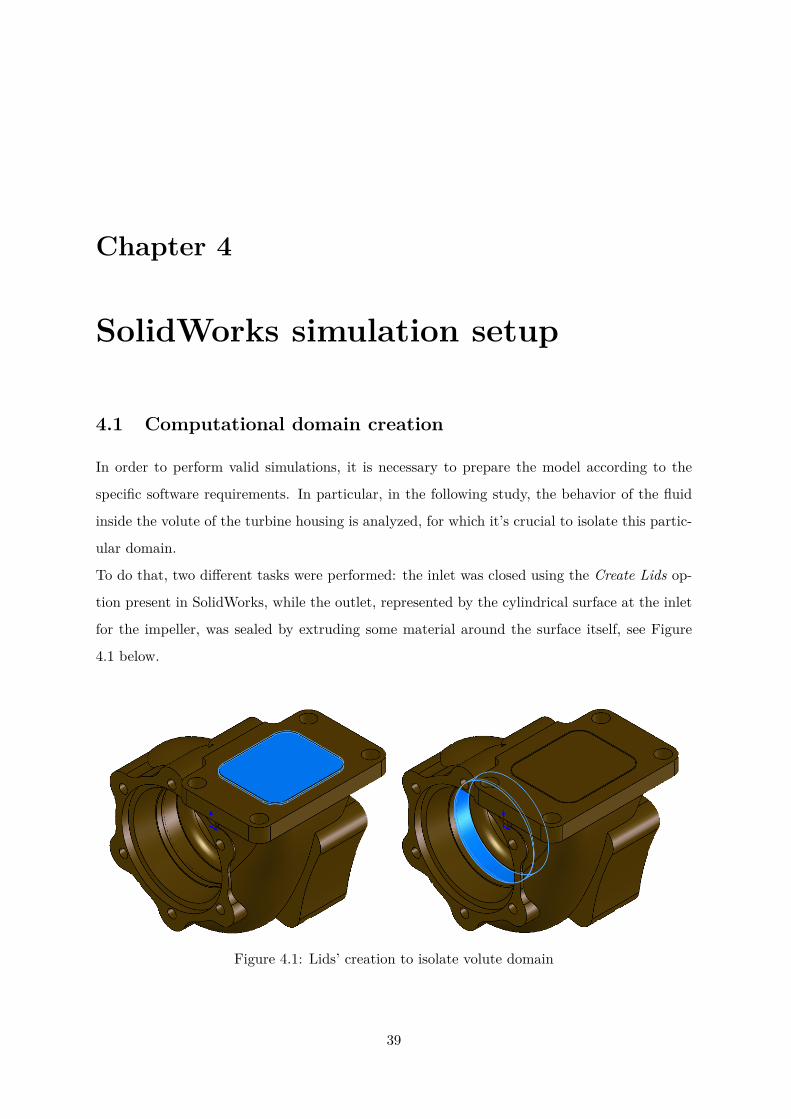
4.1 Computational domain creation
In order to perform valid simulations, it is necessary to prepare the model according to the
specific software requirements. In particular, in the following study, the behavior of the fluid
inside the volute of the turbine housing is analyzed, for which it’s crucial to isolate this partic-
ular domain.
To do that, two different tasks were performed: the inlet was closed using the Create Lids op-
tion present in SolidWorks, while the outlet, represented by the cylindrical surface at the inlet
for the impeller, was sealed by extruding some material around the surface itself, see Figure
4.1 below.
Figure 4.1: Lids’ creation to isolate volute domain
39
CHAPTER 4. SOLIDWORKS SIMULATION SETUP
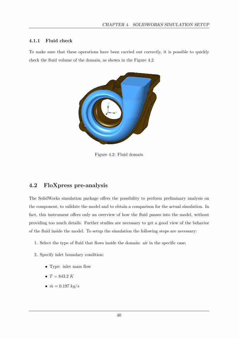
4.1.1 Fluid check
To make sure that these operations have been carried out correctly, it is possible to quickly
check the fluid volume of the domain, as shown in the Figure 4.2.
Figure 4.2: Fluid domain
4.2 FloXpress pre-analysis
The SolidWorks simulation package offers the possibility to perform preliminary analysis on
the component, to validate the model and to obtain a comparison for the actual simulation. In
fact, this instrument offers only an overview of how the fluid passes into the model, without
providing too much details. Further studies are necessary to get a good view of the behavior
of the fluid inside the model. To setup the simulation the following steps are necessary:
1. Select the type of fluid that flows inside the domain: air in the specific case;
2. Specify inlet boundary condition:
• Type: inlet mass flow
• T = 843.2 K
• m = 0.197 kg/s
40
CHAPTER 4. SOLIDWORKS SIMULATION SETUP
3. Specify outlet boundary condition:
• Type: static pressure
• p = 220000 Pa
4. Solve the model.
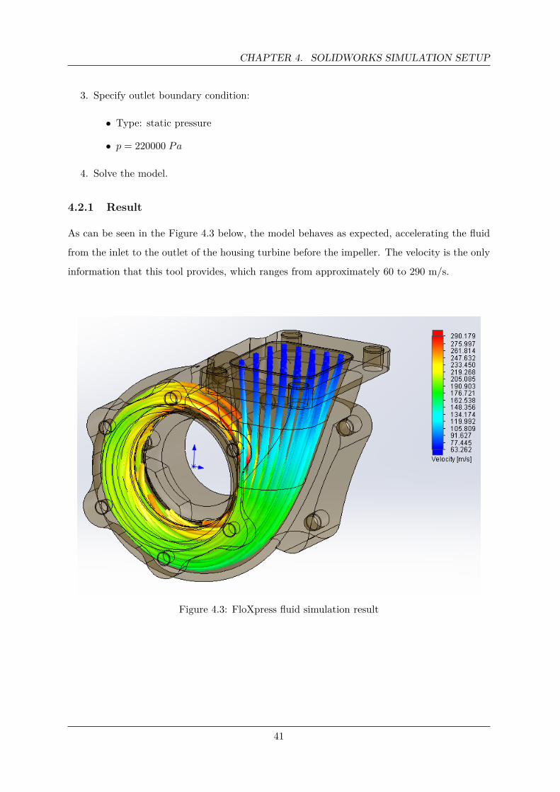
4.2.1 Result
As can be seen in the Figure 4.3 below, the model behaves as expected, accelerating the fluid
from the inlet to the outlet of the housing turbine before the impeller. The velocity is the only
information that this tool provides, which ranges from approximately 60 to 290 m/s.
Figure 4.3: FloXpress fluid simulation result
41
CHAPTER 4. SOLIDWORKS SIMULATION SETUP
4.3 Flow Simulation
Through this tool it is possible to carry out more in-depth investigations and go into more detail
regarding the study of the flow, as well as the possibility of obtaining a greater number of results
and outcomes. In fact, it is possible to obtain information on pressure, speed, temperature,
enthalpy and Mach number thanks to the resolution of the NS and basic thermodynamics
equations implemented by the software and discussed in Chapter 2.
Obviously this type of analysis requires a more detailed preparation and setup of the model,
choosing from the type of simulation that one intends to carry out, e.g., internal, external,
static or dynamic up to the type of fluid that intended to study, such as air or in the specific
case exhaust gases. As previously done, it is necessary to first isolate the fluid domain and then
define the type of simulation to be carried out (tasks described in paragraphs 4.1 and 4.1.1).
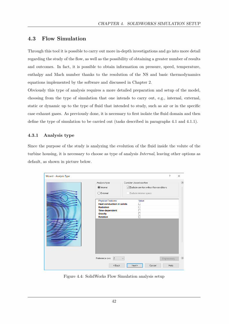
4.3.1 Analysis type
Since the purpose of the study is analyzing the evolution of the fluid inside the volute of the
turbine housing, it is necessary to choose as type of analysis Internal, leaving other options as
default, as shown in picture below.
Figure 4.4: SolidWorks Flow Simulation analysis setup
42
CHAPTER 4. SOLIDWORKS SIMULATION SETUP
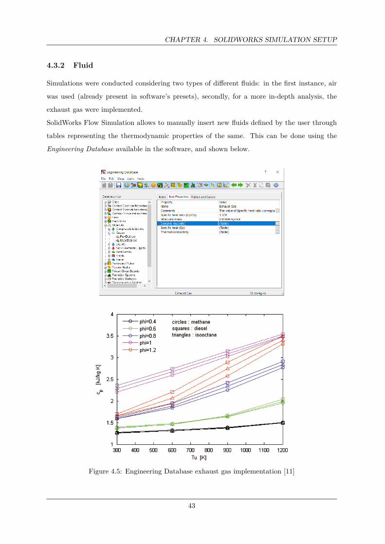
4.3.2 Fluid
Simulations were conducted considering two types of different fluids: in the first instance, air
was used (already present in software’s presets), secondly, for a more in-depth analysis, the
exhaust gas were implemented.
SolidWorks Flow Simulation allows to manually insert new fluids defined by the user through
tables representing the thermodynamic properties of the same. This can be done using the
Engineering Database available in the software, and shown below.
Figure 4.5: Engineering Database exhaust gas implementation [11]
43
CHAPTER 4. SOLIDWORKS SIMULATION SETUP
Values such as the Specific Heat Ratio or the Molecular mass can be defined as a singular input;
others like Dynamic viscosity, Specific heat or Thermal conductivity are defined using look-up
tables or specific charts (Figure 4.5). In particular k = cp
cv= 1.335 kJ/kgK while the molecular
mass m = 0.02896 kg/mol.
4.3.3 Wall and initial conditions
As regards this setting, the software allows to set two different parameters: Default wall thermal
condition and Roughness.
Default wall thermal condition
In this case it is possible to choose between different options: Adiabatic wall, Heat flux, Heat
transfer rate, Wall temperature.
As part of this simulation, the first and last options were used so that a comparison of results
can be made.
Roughness
Here it is possible to set the roughness of the surfaces touched by the fluid and expressed in
micrometers. Even in this case the value will be changed in order to present a greater overview
of results and working conditions.
Initial conditions
As well as described in the other paragraphs, here it is also possible to set the initial conditions
of the fluid, such as its pressure and temperature or the input speed.
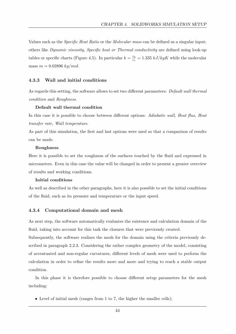
4.3.4 Computational domain and mesh
As next step, the software automatically evaluates the existence and calculation domain of the
fluid, taking into account for this task the closures that were previously created.
Subsequently, the software realizes the mesh for the domain using the criteria previously de-
scribed in paragraph 2.2.3. Considering the rather complex geometry of the model, consisting
of accentuated and non-regular curvatures, different levels of mesh were used to perform the
calculation in order to refine the results more and more and trying to reach a stable output
condition.
In this phase it is therefore possible to choose different setup parameters for the mesh
including:
• Level of initial mesh (ranges from 1 to 7, the higher the smaller cells);
44
CHAPTER 4. SOLIDWORKS SIMULATION SETUP
• Minimum gap size;
• Number of cells in each x, y, z directions;
• Advanced channel refinement option.
Figure 4.6: Mesh and Computational Domain visualization
4.3.5 Boundary conditions
In the model under investigation, two main BC’s have been set in order to perform calculations:
A pressure opening boundary condition, which can be static pressure, or total pressure, or
environment pressure is imposed in the general case when the flow direction and/or magnitude
at the model opening are not known a priori, so they are to be calculated as part of the solution.
Which of these parameters is specified depends on which one of them is known.
A flow opening boundary condition is imposed when dynamic flow properties (i.e., the flow
direction and mass/volume flow rate or velocity/Mach number) are known at the opening. If
the flow enters the model, then the inlet temperature, fluid mixture composition and turbulence
parameters must be specified also. The pressure at the opening will be determined as part of
the solution.
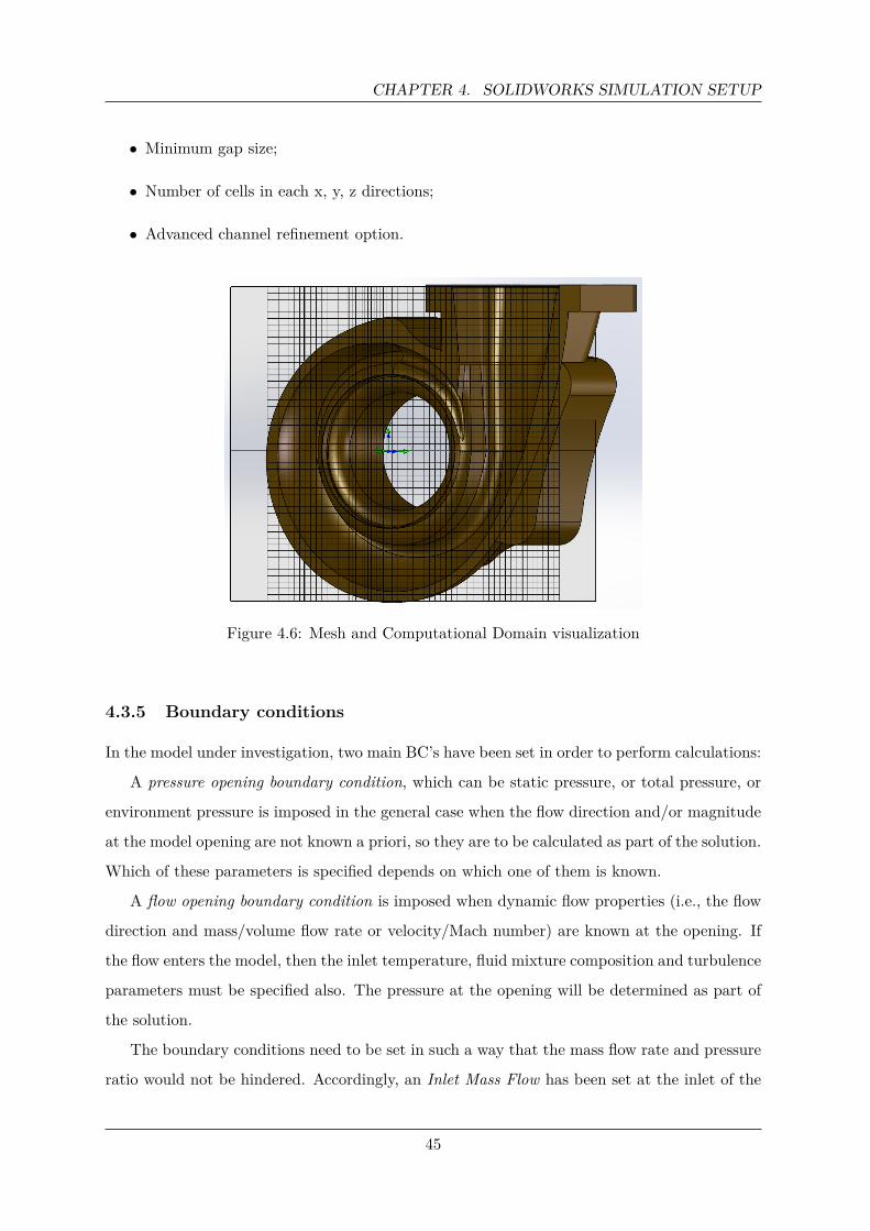
The boundary conditions need to be set in such a way that the mass flow rate and pressure
ratio would not be hindered. Accordingly, an Inlet Mass Flow has been set at the inlet of the
45
CHAPTER 4. SOLIDWORKS SIMULATION SETUP
turbine housing, while a Static Pressure at the outlet (inlet for the impeller of the tubine).
See paragraph 3.2 for data reference.
Figure 4.7: Boundary conditions setup
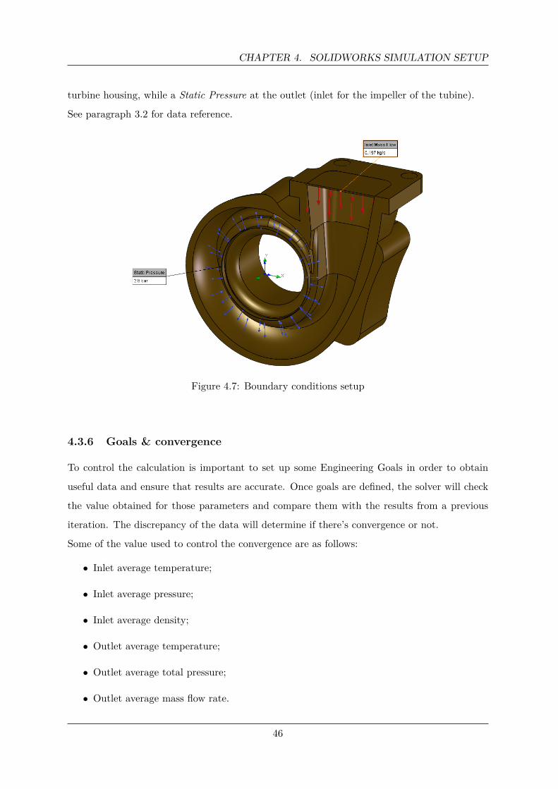
4.3.6 Goals & convergence
To control the calculation is important to set up some Engineering Goals in order to obtain
useful data and ensure that results are accurate. Once goals are defined, the solver will check
the value obtained for those parameters and compare them with the results from a previous
iteration. The discrepancy of the data will determine if there’s convergence or not.
Some of the value used to control the convergence are as follows:
• Inlet average temperature;
• Inlet average pressure;
• Inlet average density;
• Outlet average temperature;
• Outlet average total pressure;
• Outlet average mass flow rate.
46
Chapter 5
SolidWorks - Calculations
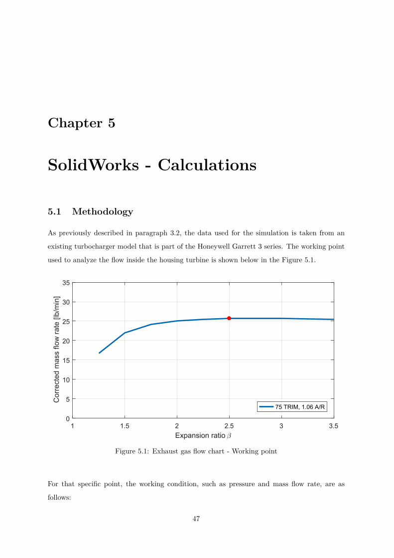
5.1 Methodology
As previously described in paragraph 3.2, the data used for the simulation is taken from an
existing turbocharger model that is part of the Honeywell Garrett 3 series. The working point
used to analyze the flow inside the housing turbine is shown below in the Figure 5.1.
1 1.5 2 2.5 3 3.5Expansion ratio
0
5
10
15
20
25
30
35
Cor
rect
ed m
ass
flow
rate
[lb/
min
]
75 TRIM, 1.06 A/R
Figure 5.1: Exhaust gas flow chart - Working point
For that specific point, the working condition, such as pressure and mass flow rate, are as
follows:
47
CHAPTER 5. SOLIDWORKS - CALCULATIONS
• Pressure ratio: β = 2.5
• Mass flow: m = 26 lb/min = 0.197 kg/s
Since the simulations carried out do not involve the turbine impeller, but only the volute
that has the task of accelerating the exhaust gases, converting part of the energy of pressure
into kinetic energy, the objective to achieve was that of finding the pressure and the average
speed of the fluid at the turbine housing inlet, in order to develop that specific expansion ratio.
The turbine expansion ratio β is defined as the ratio between the pressure at the inlet of the
turbine housing (p3) and the pressure at the output of the impeller (p4). Therefore, considering
a value of p4 ' 115000 Pa (1.15 bar), the pressure at the inlet of the turbine housing must be
equal to p3 ' 285000 Pa (2.85 bar).
β = p3
p4= 2.5 → p3 = β · p4 ' 285000 Pa = 2.85 bar (5.1)
5.2 Results
To achieve this result, different working conditions were simulated, gradually changing the
pressure at the inlet of the impeller until the desired result is gained. With this setting, the
software calculates for subsequent iterations the inlet pressure in the turbine, solving the equa-
tions discussed in Chapter 2.
Pressure Impeller inlet [Pa] Turbine housing inlet [Pa]
#1 2.00 · 105 2.24 · 105
#2 2.10 · 105 2.33 · 105
#3 2.25 · 105 2.47 · 105
#4 2.40 · 105 2.60 · 105
#5 2.60 · 105 2.85 · 105
Table 5.1: Pressures iteration at domain’s boundary
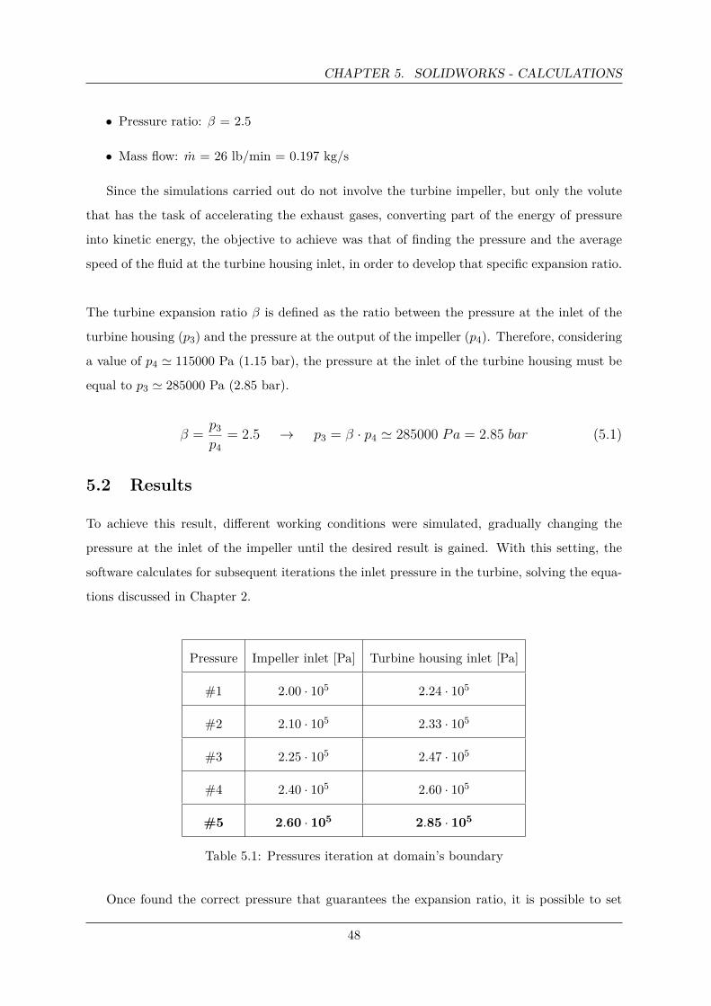
Once found the correct pressure that guarantees the expansion ratio, it is possible to set
48
CHAPTER 5. SOLIDWORKS - CALCULATIONS
the boundary conditions (as shown in Figure 5.2) and proceed with the calculations of other
parameters.
Figure 5.2: Boundary conditions setup
• Turbine housing inlet: Inlet mass flow, m = 0.197 kg/s 285000 Pa, T = 823 K = 550 C;
• Impeller inlet: Static pressure, p = 260000 Pa.
Then, simulations have been gradually refined, increasing step by step the mesh parameter,
thus reducing the size of the element and improving the accuracy of the results, which are
presented below by differentiating the two types of fluid used.
5.2.1 Fluid - Air
The results achieved using the software preset Air are quite good, however it is advisable to
use the data of the exhaust gases for greater accuracy even if a certain variance of the data is
always present. The results are shown in charts below.
49
CHAPTER 5. SOLIDWORKS - CALCULATIONS
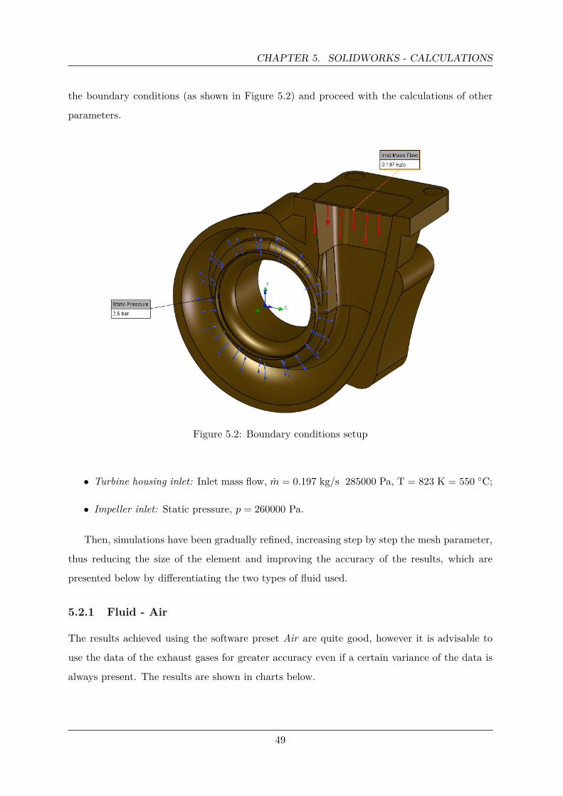
As it is visible from the graphs as the mesh is refined, the results tend to stabilize and
converge.
2,78
2,80
2,82
2,84
2,86
2,88
2,90
2,92
2,94
Minimum Maximum Bulk Average
Pre
ssu
re [
bar
]
Pressure turbine housing inlet
Mesh 3 AIR
Mesh 5 AIR
Mesh 7 AIR
Mesh 7 AIR refined
Figure 5.3: Pressure results using Air as simulation fluid
0
50
100
150
200
250
Minimum Maximum Bulk Average
Vel
oci
ty [
m/s
]
Outlet Velocity
Mesh 3 AIR
Mesh 5 AIR
Mesh 7 AIR
Mesh 7 AIR refined
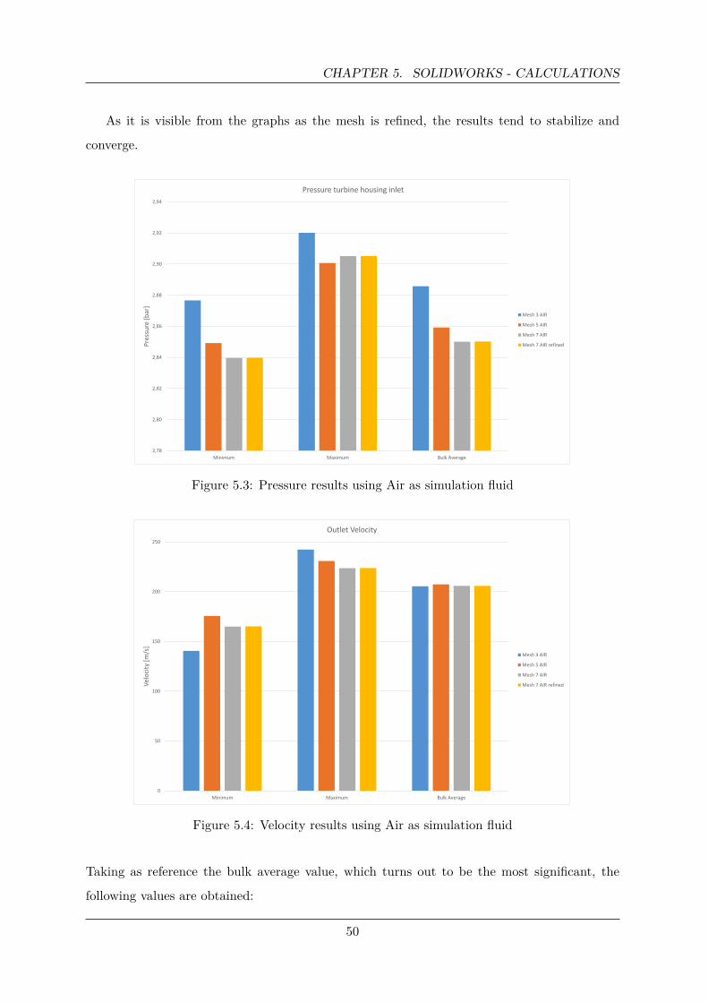
Figure 5.4: Velocity results using Air as simulation fluid
Taking as reference the bulk average value, which turns out to be the most significant, the
following values are obtained:
50
CHAPTER 5. SOLIDWORKS - CALCULATIONS
• Pressure at turbine housing inlet: 2.85 · 105 Pa = 2.85 bar, which is consistent with
value obtained with the previous calculations;
• Outlet velocity: ' 206 m/s. The software also calculated the velocity at the inlet of the
turbine housing in ' 55.5 m/s
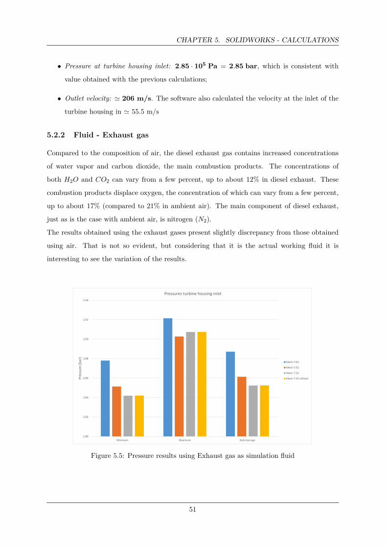
5.2.2 Fluid - Exhaust gas
Compared to the composition of air, the diesel exhaust gas contains increased concentrations
of water vapor and carbon dioxide, the main combustion products. The concentrations of
both H2O and CO2 can vary from a few percent, up to about 12% in diesel exhaust. These
combustion products displace oxygen, the concentration of which can vary from a few percent,
up to about 17% (compared to 21% in ambient air). The main component of diesel exhaust,
just as is the case with ambient air, is nitrogen (N2).
The results obtained using the exhaust gases present slightly discrepancy from those obtained
using air. That is not so evident, but considering that it is the actual working fluid it is
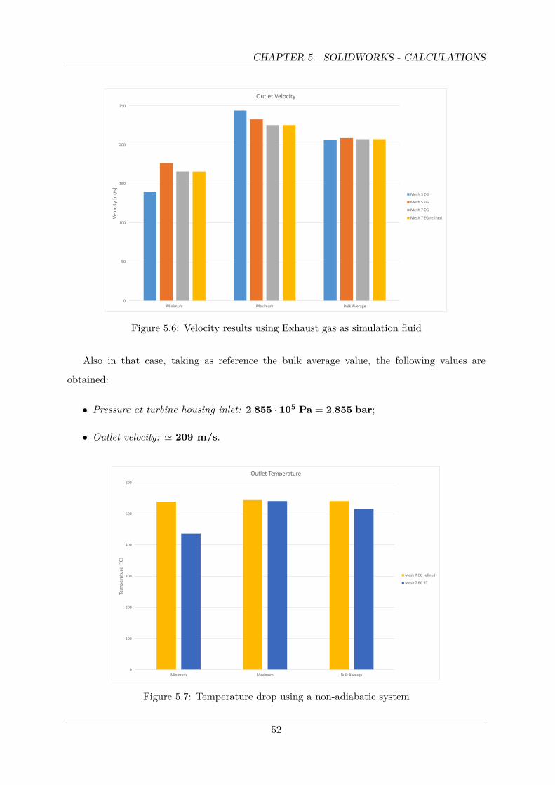
interesting to see the variation of the results.
2,80
2,82
2,84
2,86
2,88
2,90
2,92
2,94
Minimum Maximum Bulk Average
Pre
ssu
re [
bar
]
Pressures turbine housing inlet
Mesh 3 EG
Mesh 5 EG
Mesh 7 EG
Mesh 7 EG refined
Figure 5.5: Pressure results using Exhaust gas as simulation fluid
51
CHAPTER 5. SOLIDWORKS - CALCULATIONS
0
50
100
150
200
250
Minimum Maximum Bulk Average
Vel
oci
ty [
m/s
]
Outlet Velocity
Mesh 3 EG
Mesh 5 EG
Mesh 7 EG
Mesh 7 EG refined
Figure 5.6: Velocity results using Exhaust gas as simulation fluid
Also in that case, taking as reference the bulk average value, the following values are
obtained:
• Pressure at turbine housing inlet: 2.855 · 105 Pa = 2.855 bar;
• Outlet velocity: ' 209 m/s.
0
100
200
300
400
500
600
Minimum Maximum Bulk Average
Tem
per
atu
re [
°C]
Outlet Temperature
Mesh 7 EG refined
Mesh 7 EG RT
Figure 5.7: Temperature drop using a non-adiabatic system
52
CHAPTER 5. SOLIDWORKS - CALCULATIONS
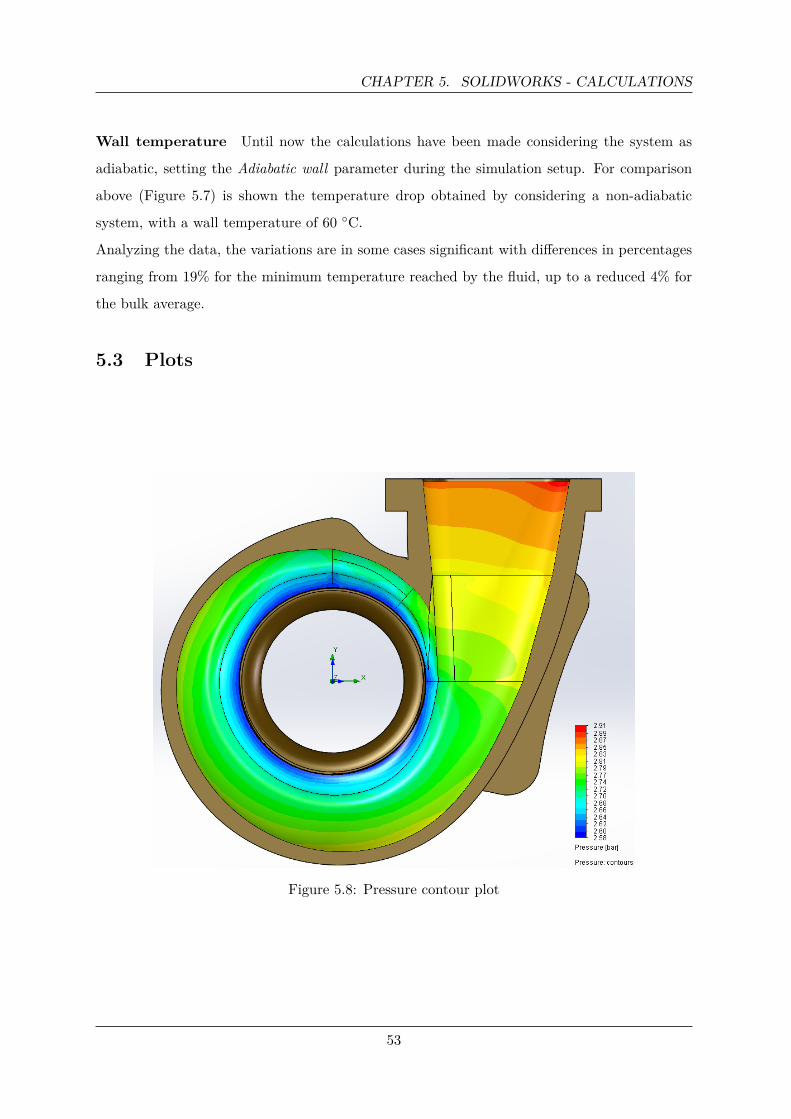
Wall temperature Until now the calculations have been made considering the system as
adiabatic, setting the Adiabatic wall parameter during the simulation setup. For comparison
above (Figure 5.7) is shown the temperature drop obtained by considering a non-adiabatic
system, with a wall temperature of 60 C.
Analyzing the data, the variations are in some cases significant with differences in percentages
ranging from 19% for the minimum temperature reached by the fluid, up to a reduced 4% for
the bulk average.
5.3 Plots
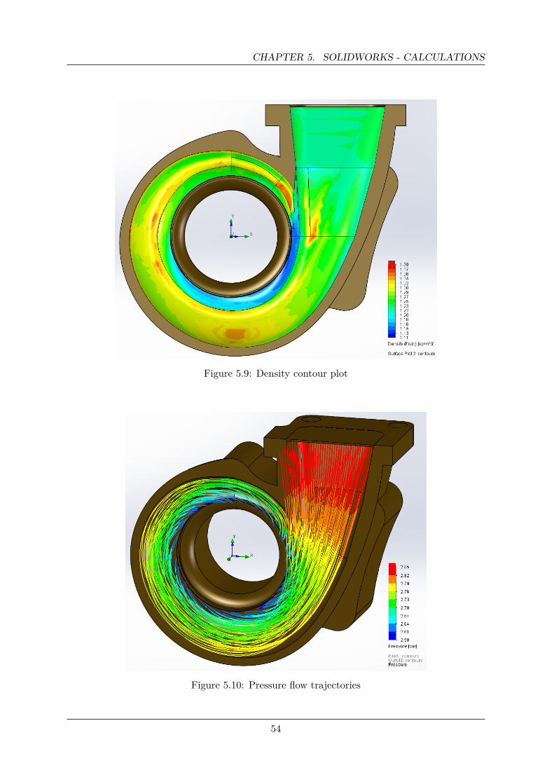
Figure 5.8: Pressure contour plot
53
CHAPTER 5. SOLIDWORKS - CALCULATIONS
Figure 5.9: Density contour plot
Figure 5.10: Pressure flow trajectories
54
CHAPTER 5. SOLIDWORKS - CALCULATIONS
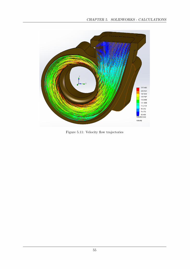
Figure 5.11: Velocity flow trajectories
55
Chapter 6
GT-Power engine model
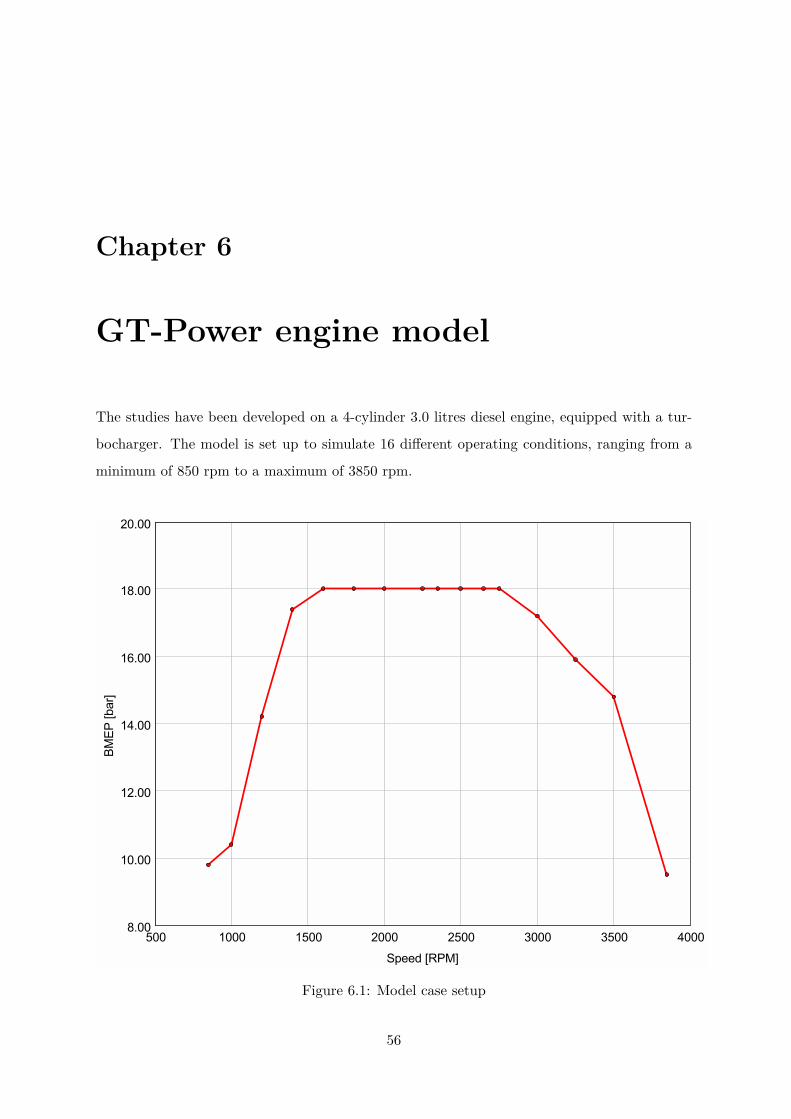
The studies have been developed on a 4-cylinder 3.0 litres diesel engine, equipped with a tur-
bocharger. The model is set up to simulate 16 different operating conditions, ranging from a
minimum of 850 rpm to a maximum of 3850 rpm.
Figure 6.1: Model case setup
56
CHAPTER 6. GT-POWER ENGINE MODEL
Case #1 #2 #3 #4 #5 #6 #7 #8
rpm 850 1000 1200 1400 1600 1800 2000 2250
bmep 9.80 10.40 14.20 17.40 18.00 18.00 18.00 18.00
Case #9 #10 #11 #12 #13 #14 #15 #16
rpm 2350 2500 2650 2750 3000 3250 3500 3850
bmep 18.00 18.00 18.00 18.00 17.20 15.90 14.80 9.50
Table 6.1: Case setup working points
6.1 Internal combustion engine
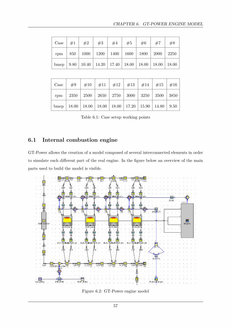
GT-Power allows the creation of a model composed of several interconnected elements in order
to simulate each different part of the real engine. In the figure below an overview of the main
parts used to build the model is visible.
Figure 6.2: GT-Power engine model
57
CHAPTER 6. GT-POWER ENGINE MODEL
The model can be divided into different areas according to the type of process they will
simulate:
• combustion process, thermal and fluid-dynamic simulation is associated with the 4 cylin-
ders, injectors, intake and exhaust valves and manifolds as well as EGR system, visible
in the middle and left-hand side of the picture;
• mechanics and dynamics of the engine is processed by the Engine CrankTrain element
visible on the right-hand side.
In addition, a series of PID controllers are required to achieve convergence towards the
desired solution: starting from first attempt value (read from case setup), these act in closed
loop modifying the process parameters adapting to the needs of the system. The main one
is the Load PID which imposes the amount of injected fuel, comparing the effective pressure
calculated during the previous cycle with the goal to be achieved.
6.2 Turbocharger
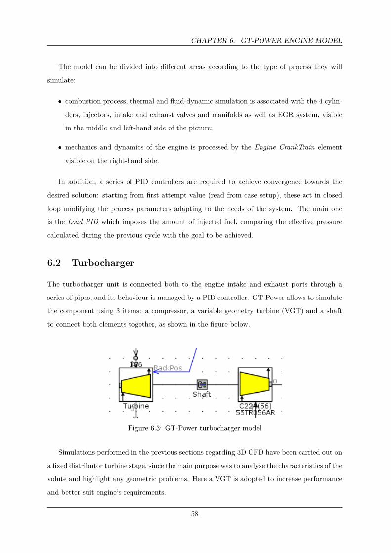
The turbocharger unit is connected both to the engine intake and exhaust ports through a
series of pipes, and its behaviour is managed by a PID controller. GT-Power allows to simulate
the component using 3 items: a compressor, a variable geometry turbine (VGT) and a shaft
to connect both elements together, as shown in the figure below.
Figure 6.3: GT-Power turbocharger model
Simulations performed in the previous sections regarding 3D CFD have been carried out on
a fixed distributor turbine stage, since the main purpose was to analyze the characteristics of the
volute and highlight any geometric problems. Here a VGT is adopted to increase performance
and better suit engine’s requirements.
58
CHAPTER 6. GT-POWER ENGINE MODEL
Because of that, multiple turbine performance maps are required to the solver, one for each
different rack position. In that specific case 6 maps were provided which are not enough to
properly solve the system. The software in fact interpolates given values to get a full view of
turbine performance along all rack position range. Then using a PID controller the value is
continuously varied to achieve the target boost pressure. If the pressure results higher than
the target, the PID opens the rack increasing turbine’s permeability and reducing the boost;
likewise, if the pressure delivered by the compressor is lower, the rack is closed increasing
turbine inlet pressure and generating more power.
6.3 Standard turbine simulation
Initial tests were performed using the standard turbine, as well as simulated on SolidWorks
by 3D CFD, to analyze and evaluate the response and performance of the engine. In order to
do that, case setup was populated with data from Table 6.1 and other values relevant for the
simulation. Results are summarized in Table 6.2.
Case RPM Power [kW ] Rack position BSFC [g/kWh] Efficiency
#1 850 20.8 0.428 233.73 0.356#2 1000 26.0 0.417 225.60 0.369#3 1200 42.6 0.363 217.35 0.383#4 1400 60.9 0.359 211.25 0.394
#5 1600 72.0 0.335 210.88 0.395#6 1800 81.0 0.401 205.80 0.404#7 2000 90.0 0.403 205.19 0.406#8 2250 101.2 0.412 205.56 0.405
#9 2350 105.7 0.430 206.56 0.403#10 2500 112.4 0.462 208.19 0.400#11 2650 119.2 0.506 209.98 0.396#12 2750 123.7 0.533 211.71 0.393
#13 3000 128.9 0.561 215.20 0.387#14 3250 129.1 0.581 219.87 0.379#15 3500 129.4 0.589 224.57 0.371#16 3850 91.4 0.633 238.90 0.348
Table 6.2: Standard turbine simulation results
59
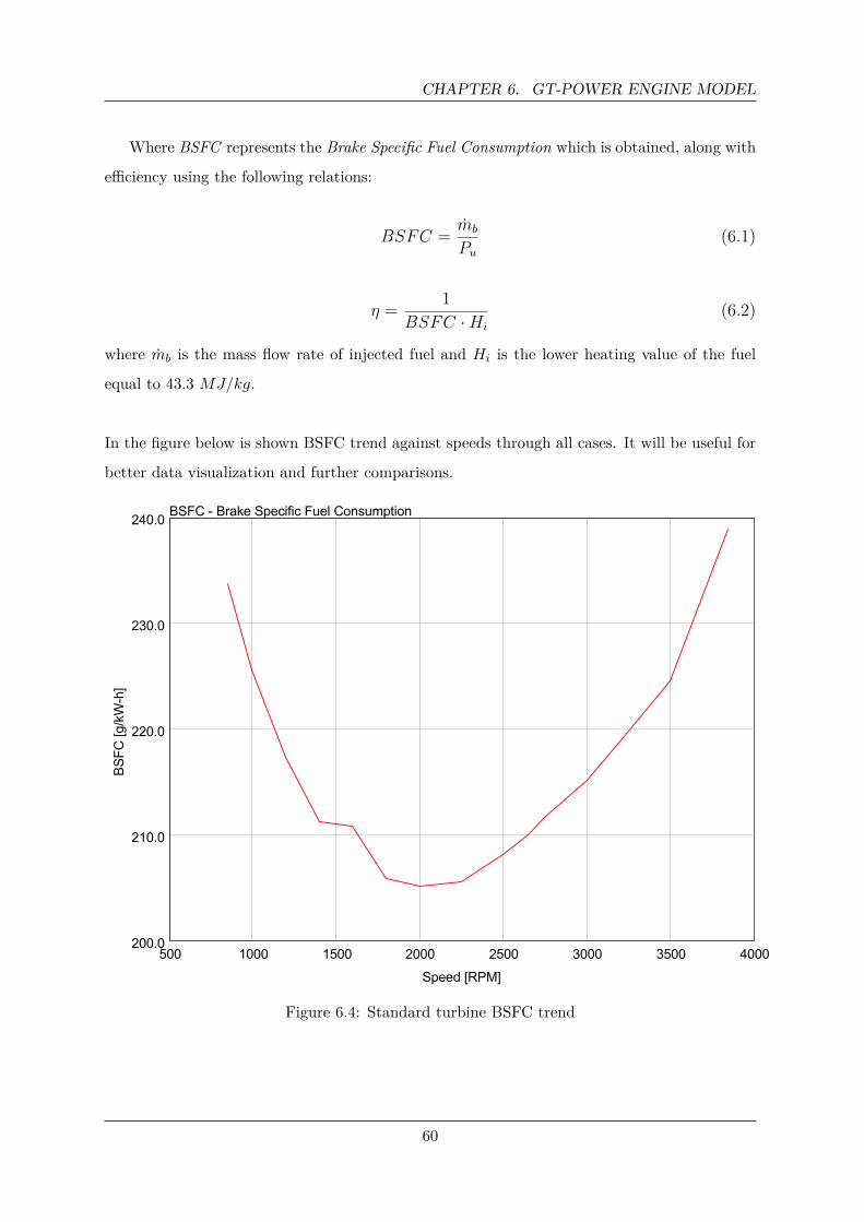
CHAPTER 6. GT-POWER ENGINE MODEL
Where BSFC represents the Brake Specific Fuel Consumption which is obtained, along with
efficiency using the following relations:
BSFC = mb
Pu(6.1)
η = 1BSFC ·Hi
(6.2)
where mb is the mass flow rate of injected fuel and Hi is the lower heating value of the fuel
equal to 43.3 MJ/kg.
In the figure below is shown BSFC trend against speeds through all cases. It will be useful for
better data visualization and further comparisons.
Figure 6.4: Standard turbine BSFC trend
60
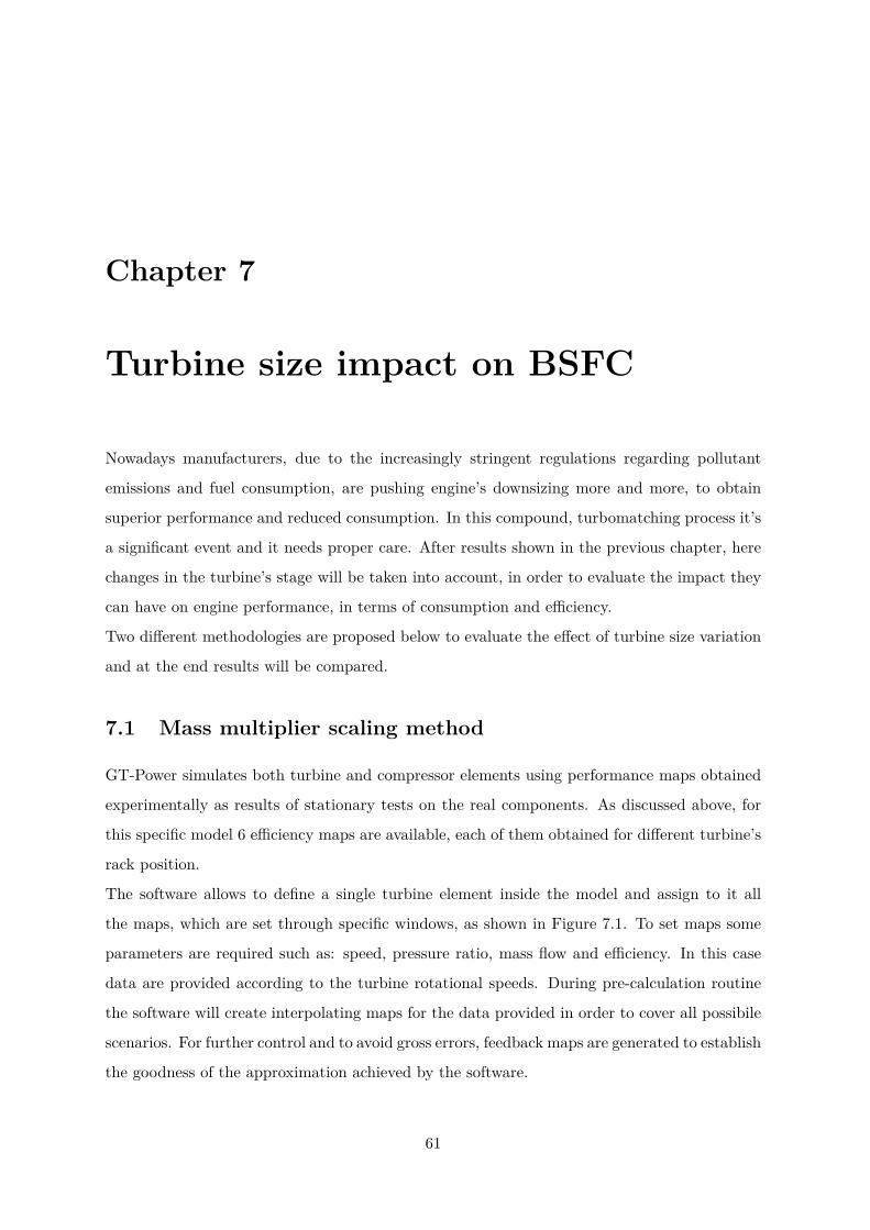
Chapter 7
Turbine size impact on BSFC
Nowadays manufacturers, due to the increasingly stringent regulations regarding pollutant
emissions and fuel consumption, are pushing engine’s downsizing more and more, to obtain
superior performance and reduced consumption. In this compound, turbomatching process it’s
a significant event and it needs proper care. After results shown in the previous chapter, here
changes in the turbine’s stage will be taken into account, in order to evaluate the impact they
can have on engine performance, in terms of consumption and efficiency.
Two different methodologies are proposed below to evaluate the effect of turbine size variation
and at the end results will be compared.
7.1 Mass multiplier scaling method
GT-Power simulates both turbine and compressor elements using performance maps obtained
experimentally as results of stationary tests on the real components. As discussed above, for
this specific model 6 efficiency maps are available, each of them obtained for different turbine’s
rack position.
The software allows to define a single turbine element inside the model and assign to it all
the maps, which are set through specific windows, as shown in Figure 7.1. To set maps some
parameters are required such as: speed, pressure ratio, mass flow and efficiency. In this case
data are provided according to the turbine rotational speeds. During pre-calculation routine
the software will create interpolating maps for the data provided in order to cover all possibile
scenarios. For further control and to avoid gross errors, feedback maps are generated to establish
the goodness of the approximation achieved by the software.
61
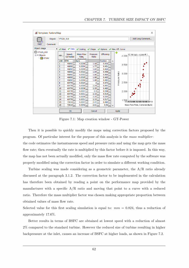
CHAPTER 7. TURBINE SIZE IMPACT ON BSFC
Figure 7.1: Map creation window - GT-Power
Then it is possible to quickly modify the maps using correction factors proposed by the
program. Of particular interest for the purpose of this analysis is the mass multiplier :
the code estimates the instantaneous speed and pressure ratio and using the map gets the mass
flow rate; then eventually the rate is multiplied by this factor before it is imposed. In this way,
the map has not been actually modified, only the mass flow rate computed by the software was
properly modified using the correction factor in order to simulate a different working condition.
Turbine scaling was made considering as a geometric parameter, the A/R ratio already
discussed at the paragraph 3.1.2. The correction factor to be implemented in the calculation
has therefore been obtained by reading a point on the performance map provided by the
manufacturer with a specific A/R ratio and moving that point to a curve with a reduced
ratio. Therefore the mass multiplier factor was chosen making appropriate proportion between
obtained values of mass flow rate.
Selected value for this first scaling simulation is equal to: mm = 0.824, thus a reduction of
approximately 17.6%.
Better results in terms of BSFC are obtained at lowest speed with a reduction of almost
2% compared to the standard turbine. However the reduced size of turbine resulting in higher
backpressure at the inlet, causes an increase of BSFC at higher loads, as shown in Figure 7.2.
62
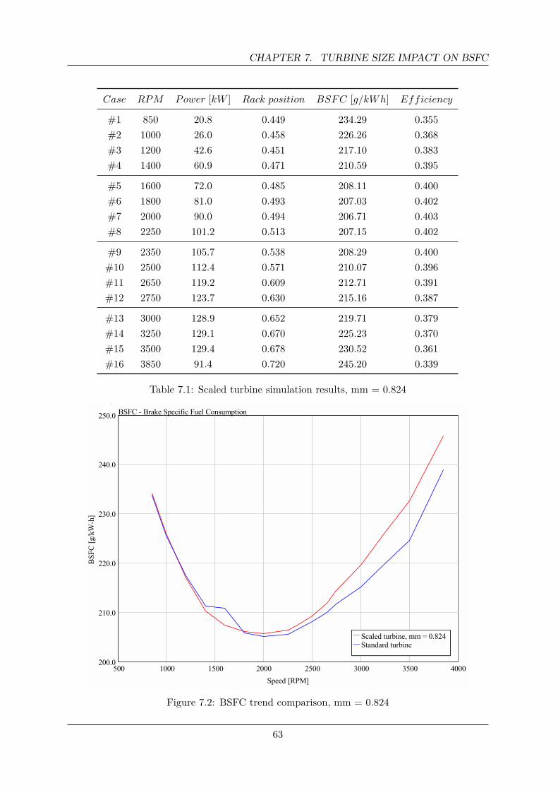
CHAPTER 7. TURBINE SIZE IMPACT ON BSFC
Case RPM Power [kW ] Rack position BSFC [g/kWh] Efficiency
#1 850 20.8 0.449 234.29 0.355#2 1000 26.0 0.458 226.26 0.368#3 1200 42.6 0.451 217.10 0.383#4 1400 60.9 0.471 210.59 0.395
#5 1600 72.0 0.485 208.11 0.400#6 1800 81.0 0.493 207.03 0.402#7 2000 90.0 0.494 206.71 0.403#8 2250 101.2 0.513 207.15 0.402
#9 2350 105.7 0.538 208.29 0.400#10 2500 112.4 0.571 210.07 0.396#11 2650 119.2 0.609 212.71 0.391#12 2750 123.7 0.630 215.16 0.387
#13 3000 128.9 0.652 219.71 0.379#14 3250 129.1 0.670 225.23 0.370#15 3500 129.4 0.678 230.52 0.361#16 3850 91.4 0.720 245.20 0.339
Table 7.1: Scaled turbine simulation results, mm = 0.824
Figure 7.2: BSFC trend comparison, mm = 0.824
63
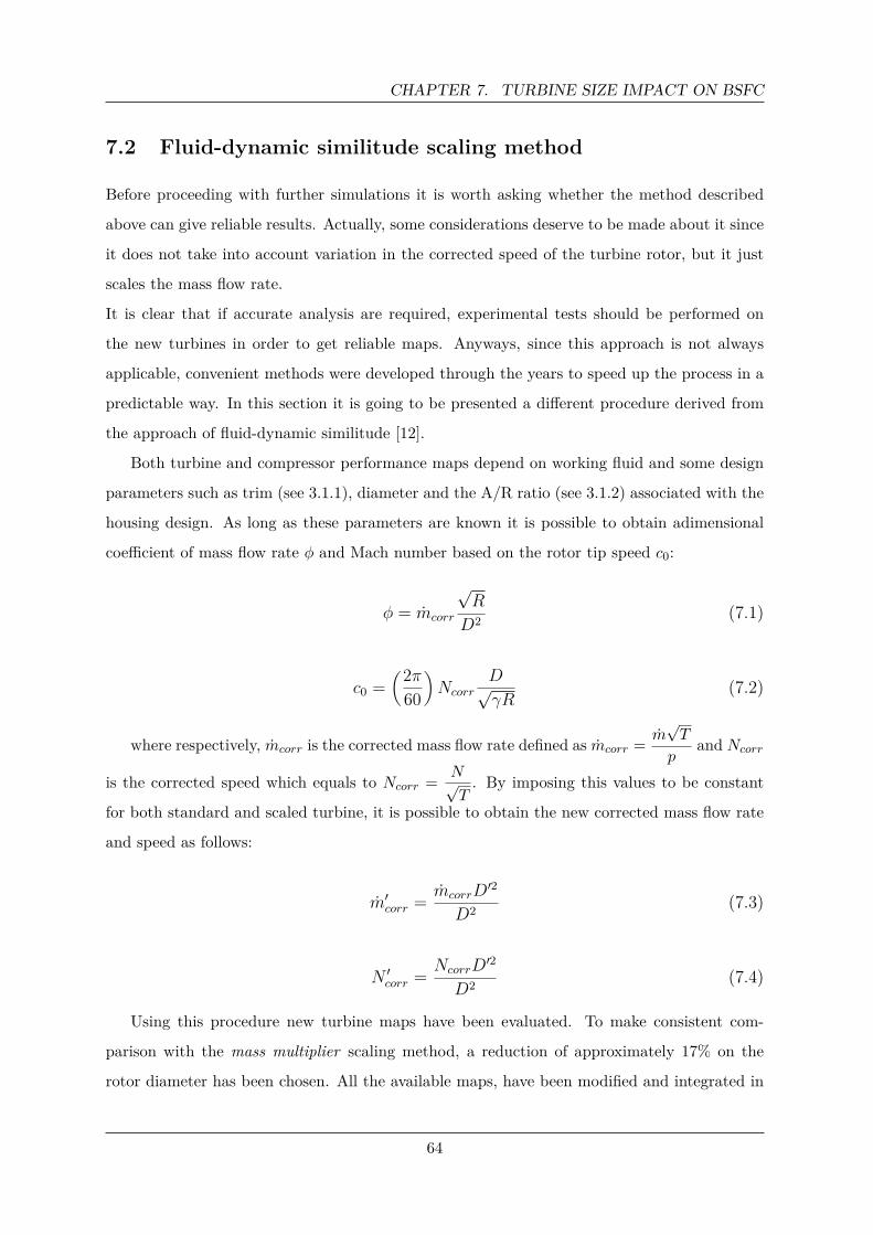
CHAPTER 7. TURBINE SIZE IMPACT ON BSFC
7.2 Fluid-dynamic similitude scaling method
Before proceeding with further simulations it is worth asking whether the method described
above can give reliable results. Actually, some considerations deserve to be made about it since
it does not take into account variation in the corrected speed of the turbine rotor, but it just
scales the mass flow rate.
It is clear that if accurate analysis are required, experimental tests should be performed on
the new turbines in order to get reliable maps. Anyways, since this approach is not always
applicable, convenient methods were developed through the years to speed up the process in a
predictable way. In this section it is going to be presented a different procedure derived from
the approach of fluid-dynamic similitude [12].
Both turbine and compressor performance maps depend on working fluid and some design
parameters such as trim (see 3.1.1), diameter and the A/R ratio (see 3.1.2) associated with the
housing design. As long as these parameters are known it is possible to obtain adimensional
coefficient of mass flow rate φ and Mach number based on the rotor tip speed c0:
φ = mcorr
√R
D2 (7.1)
c0 =(2π
60
)Ncorr
D√γR
(7.2)
where respectively, mcorr is the corrected mass flow rate defined as mcorr = m√T
pand Ncorr
is the corrected speed which equals to Ncorr = N√T
. By imposing this values to be constant
for both standard and scaled turbine, it is possible to obtain the new corrected mass flow rate
and speed as follows:
m′corr = mcorrD′2
D2 (7.3)
N ′corr = NcorrD′2
D2 (7.4)
Using this procedure new turbine maps have been evaluated. To make consistent com-
parison with the mass multiplier scaling method, a reduction of approximately 17% on the
rotor diameter has been chosen. All the available maps, have been modified and integrated in
64
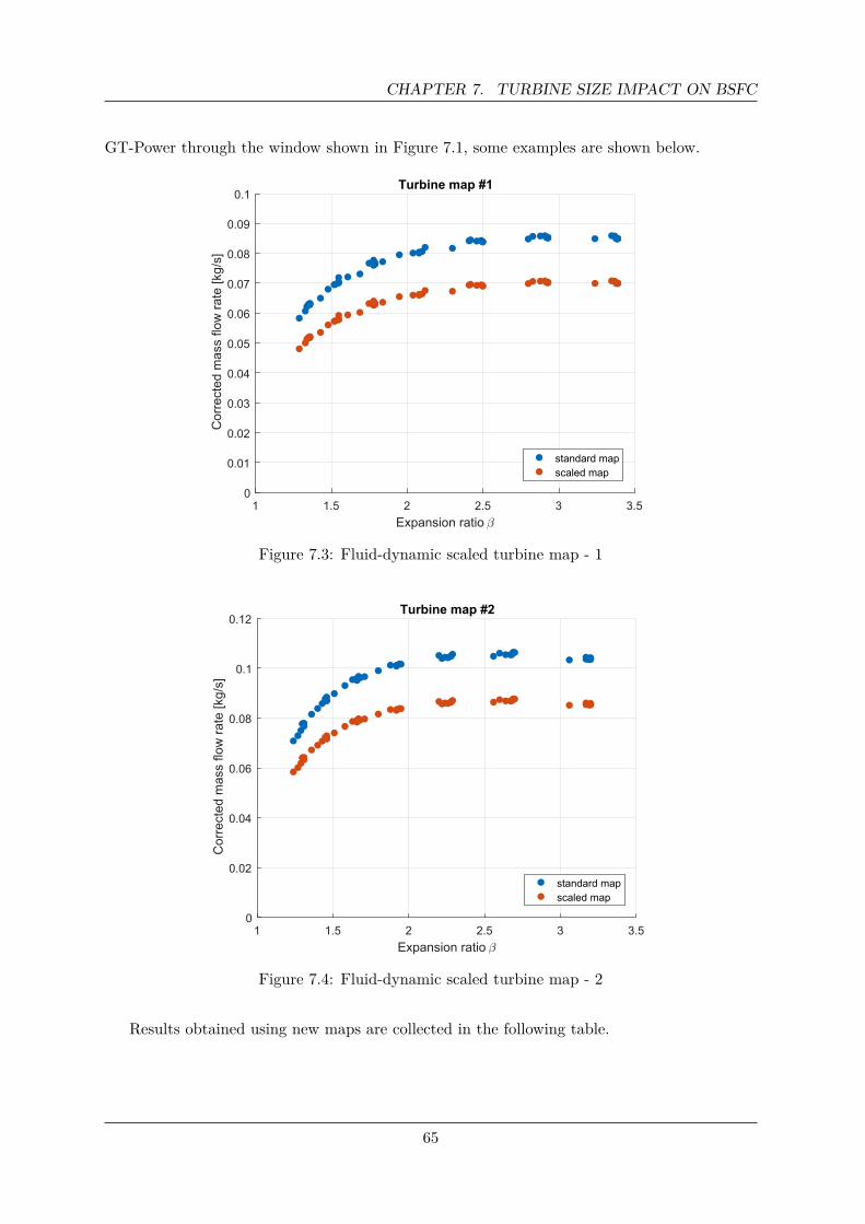
CHAPTER 7. TURBINE SIZE IMPACT ON BSFC
GT-Power through the window shown in Figure 7.1, some examples are shown below.
1 1.5 2 2.5 3 3.5Expansion ratio
0
0.01
0.02
0.03
0.04
0.05
0.06
0.07
0.08
0.09
0.1
Cor
rect
ed m
ass
flow
rate
[kg/
s]
Turbine map #1
standard mapscaled map
Figure 7.3: Fluid-dynamic scaled turbine map - 1
1 1.5 2 2.5 3 3.5Expansion ratio
0
0.02
0.04
0.06
0.08
0.1
0.12
Cor
rect
ed m
ass
flow
rate
[kg/
s]
Turbine map #2
standard mapscaled map
Figure 7.4: Fluid-dynamic scaled turbine map - 2
Results obtained using new maps are collected in the following table.
65
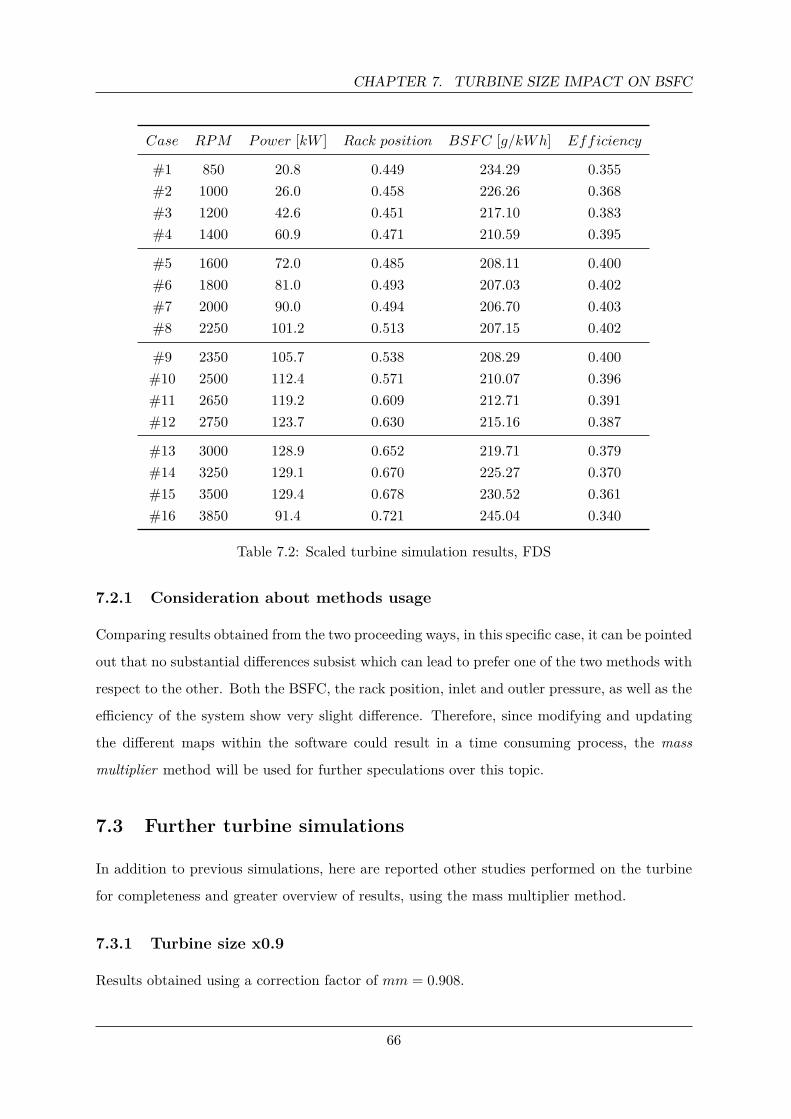
CHAPTER 7. TURBINE SIZE IMPACT ON BSFC
Case RPM Power [kW ] Rack position BSFC [g/kWh] Efficiency
#1 850 20.8 0.449 234.29 0.355#2 1000 26.0 0.458 226.26 0.368#3 1200 42.6 0.451 217.10 0.383#4 1400 60.9 0.471 210.59 0.395
#5 1600 72.0 0.485 208.11 0.400#6 1800 81.0 0.493 207.03 0.402#7 2000 90.0 0.494 206.70 0.403#8 2250 101.2 0.513 207.15 0.402
#9 2350 105.7 0.538 208.29 0.400#10 2500 112.4 0.571 210.07 0.396#11 2650 119.2 0.609 212.71 0.391#12 2750 123.7 0.630 215.16 0.387
#13 3000 128.9 0.652 219.71 0.379#14 3250 129.1 0.670 225.27 0.370#15 3500 129.4 0.678 230.52 0.361#16 3850 91.4 0.721 245.04 0.340
Table 7.2: Scaled turbine simulation results, FDS
7.2.1 Consideration about methods usage
Comparing results obtained from the two proceeding ways, in this specific case, it can be pointed
out that no substantial differences subsist which can lead to prefer one of the two methods with
respect to the other. Both the BSFC, the rack position, inlet and outler pressure, as well as the
efficiency of the system show very slight difference. Therefore, since modifying and updating
the different maps within the software could result in a time consuming process, the mass
multiplier method will be used for further speculations over this topic.
7.3 Further turbine simulations
In addition to previous simulations, here are reported other studies performed on the turbine
for completeness and greater overview of results, using the mass multiplier method.
7.3.1 Turbine size x0.9
Results obtained using a correction factor of mm = 0.908.
66
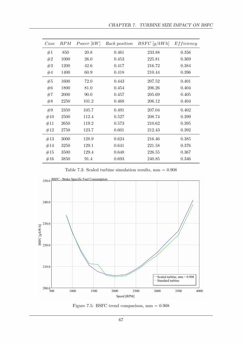
CHAPTER 7. TURBINE SIZE IMPACT ON BSFC
Case RPM Power [kW ] Rack position BSFC [g/kWh] Efficiency
#1 850 20.8 0.461 233.88 0.356#2 1000 26.0 0.453 225.81 0.369#3 1200 42.6 0.417 216.72 0.384#4 1400 60.9 0.418 210.44 0.396
#5 1600 72.0 0.443 207.52 0.401#6 1800 81.0 0.454 206.26 0.404#7 2000 90.0 0.457 205.69 0.405#8 2250 101.2 0.468 206.12 0.404
#9 2350 105.7 0.491 207.04 0.402#10 2500 112.4 0.527 208.74 0.399#11 2650 119.2 0.573 210.62 0.395#12 2750 123.7 0.601 212.43 0.392
#13 3000 128.9 0.624 216.46 0.385#14 3250 129.1 0.641 221.58 0.376#15 3500 129.4 0.648 226.55 0.367#16 3850 91.4 0.693 240.85 0.346
Table 7.3: Scaled turbine simulation results, mm = 0.908
Figure 7.5: BSFC trend comparison, mm = 0.908
67
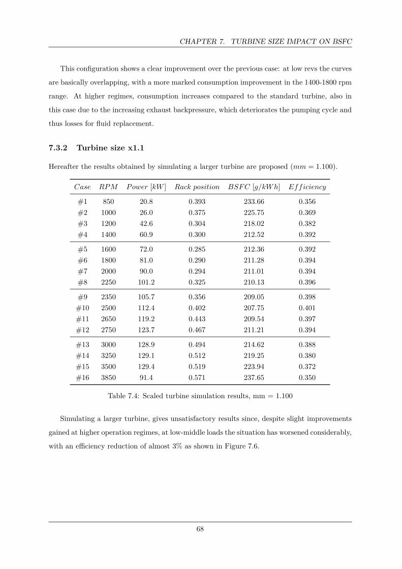
CHAPTER 7. TURBINE SIZE IMPACT ON BSFC
This configuration shows a clear improvement over the previous case: at low revs the curves
are basically overlapping, with a more marked consumption improvement in the 1400-1800 rpm
range. At higher regimes, consumption increases compared to the standard turbine, also in
this case due to the increasing exhaust backpressure, which deteriorates the pumping cycle and
thus losses for fluid replacement.
7.3.2 Turbine size x1.1
Hereafter the results obtained by simulating a larger turbine are proposed (mm = 1.100).
Case RPM Power [kW ] Rack position BSFC [g/kWh] Efficiency
#1 850 20.8 0.393 233.66 0.356#2 1000 26.0 0.375 225.75 0.369#3 1200 42.6 0.304 218.02 0.382#4 1400 60.9 0.300 212.52 0.392
#5 1600 72.0 0.285 212.36 0.392#6 1800 81.0 0.290 211.28 0.394#7 2000 90.0 0.294 211.01 0.394#8 2250 101.2 0.325 210.13 0.396
#9 2350 105.7 0.356 209.05 0.398#10 2500 112.4 0.402 207.75 0.401#11 2650 119.2 0.443 209.54 0.397#12 2750 123.7 0.467 211.21 0.394
#13 3000 128.9 0.494 214.62 0.388#14 3250 129.1 0.512 219.25 0.380#15 3500 129.4 0.519 223.94 0.372#16 3850 91.4 0.571 237.65 0.350
Table 7.4: Scaled turbine simulation results, mm = 1.100
Simulating a larger turbine, gives unsatisfactory results since, despite slight improvements
gained at higher operation regimes, at low-middle loads the situation has worsened considerably,
with an efficiency reduction of almost 3% as shown in Figure 7.6.
68
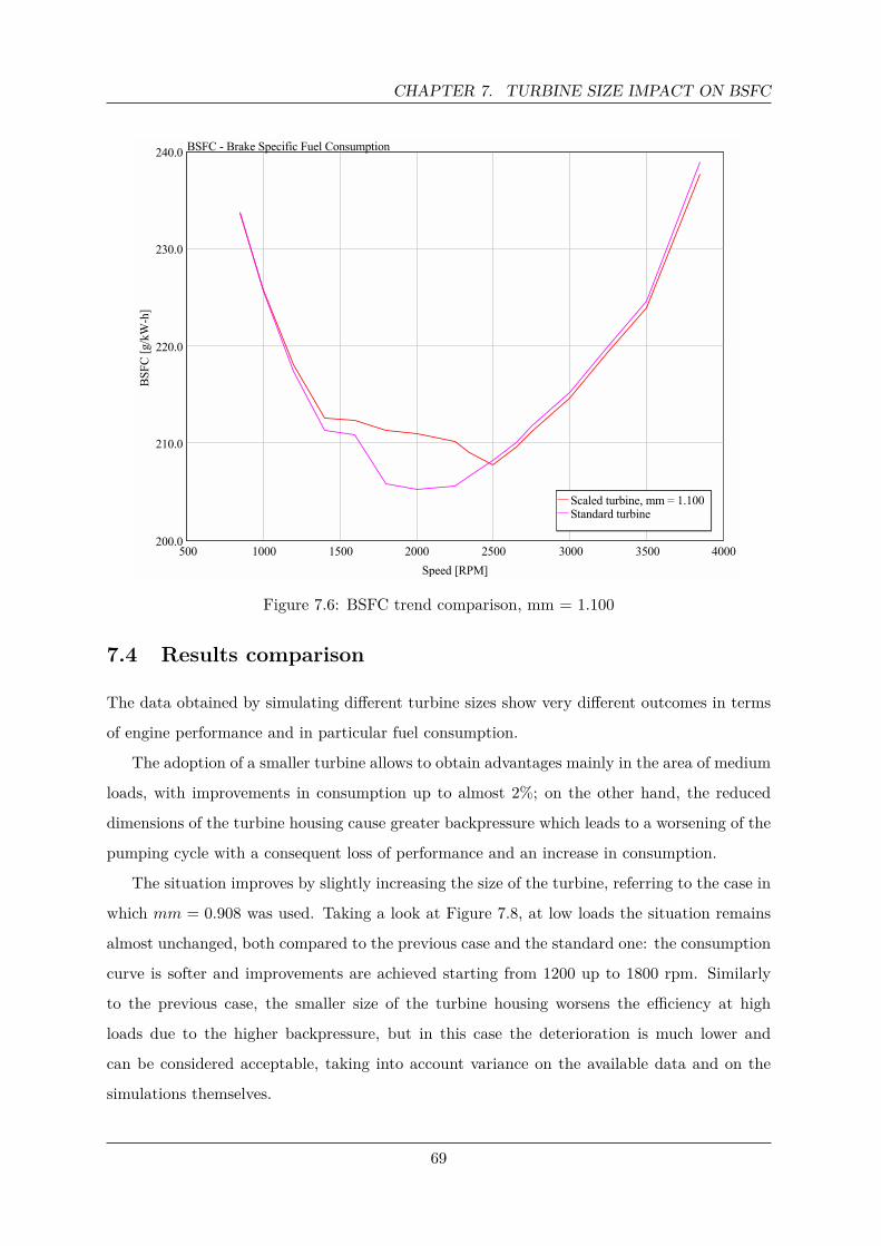
CHAPTER 7. TURBINE SIZE IMPACT ON BSFC
Figure 7.6: BSFC trend comparison, mm = 1.100
7.4 Results comparison
The data obtained by simulating different turbine sizes show very different outcomes in terms
of engine performance and in particular fuel consumption.
The adoption of a smaller turbine allows to obtain advantages mainly in the area of medium
loads, with improvements in consumption up to almost 2%; on the other hand, the reduced
dimensions of the turbine housing cause greater backpressure which leads to a worsening of the
pumping cycle with a consequent loss of performance and an increase in consumption.
The situation improves by slightly increasing the size of the turbine, referring to the case in
which mm = 0.908 was used. Taking a look at Figure 7.8, at low loads the situation remains
almost unchanged, both compared to the previous case and the standard one: the consumption
curve is softer and improvements are achieved starting from 1200 up to 1800 rpm. Similarly
to the previous case, the smaller size of the turbine housing worsens the efficiency at high
loads due to the higher backpressure, but in this case the deterioration is much lower and
can be considered acceptable, taking into account variance on the available data and on the
simulations themselves.
69
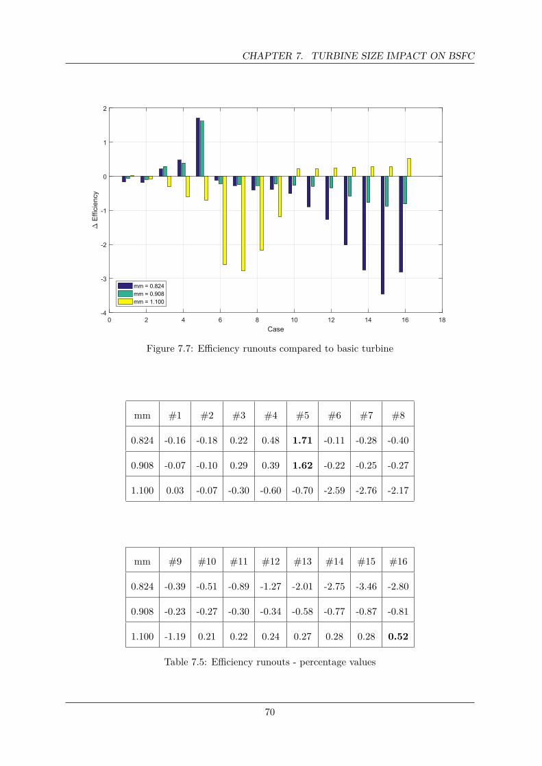
CHAPTER 7. TURBINE SIZE IMPACT ON BSFC
0 2 4 6 8 10 12 14 16 18Case
-4
-3
-2
-1
0
1
2
Effi
cien
cy
mm = 0.824mm = 0.908mm = 1.100
Figure 7.7: Efficiency runouts compared to basic turbine
mm #1 #2 #3 #4 #5 #6 #7 #8
0.824 -0.16 -0.18 0.22 0.48 1.71 -0.11 -0.28 -0.40
0.908 -0.07 -0.10 0.29 0.39 1.62 -0.22 -0.25 -0.27
1.100 0.03 -0.07 -0.30 -0.60 -0.70 -2.59 -2.76 -2.17
mm #9 #10 #11 #12 #13 #14 #15 #16
0.824 -0.39 -0.51 -0.89 -1.27 -2.01 -2.75 -3.46 -2.80
0.908 -0.23 -0.27 -0.30 -0.34 -0.58 -0.77 -0.87 -0.81
1.100 -1.19 0.21 0.22 0.24 0.27 0.28 0.28 0.52
Table 7.5: Efficiency runouts - percentage values
70
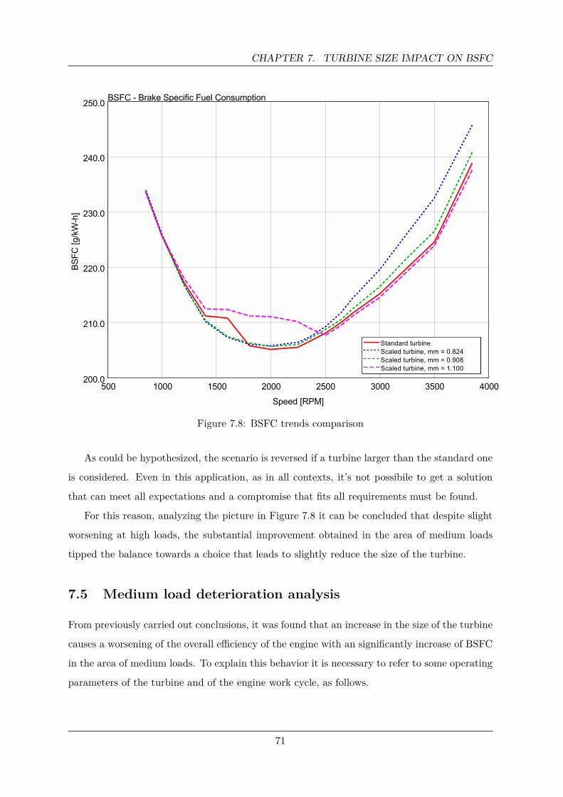
CHAPTER 7. TURBINE SIZE IMPACT ON BSFC
Figure 7.8: BSFC trends comparison
As could be hypothesized, the scenario is reversed if a turbine larger than the standard one
is considered. Even in this application, as in all contexts, it’s not possibile to get a solution
that can meet all expectations and a compromise that fits all requirements must be found.
For this reason, analyzing the picture in Figure 7.8 it can be concluded that despite slight
worsening at high loads, the substantial improvement obtained in the area of medium loads
tipped the balance towards a choice that leads to slightly reduce the size of the turbine.
7.5 Medium load deterioration analysis
From previously carried out conclusions, it was found that an increase in the size of the turbine
causes a worsening of the overall efficiency of the engine with an significantly increase of BSFC
in the area of medium loads. To explain this behavior it is necessary to refer to some operating
parameters of the turbine and of the engine work cycle, as follows.
71
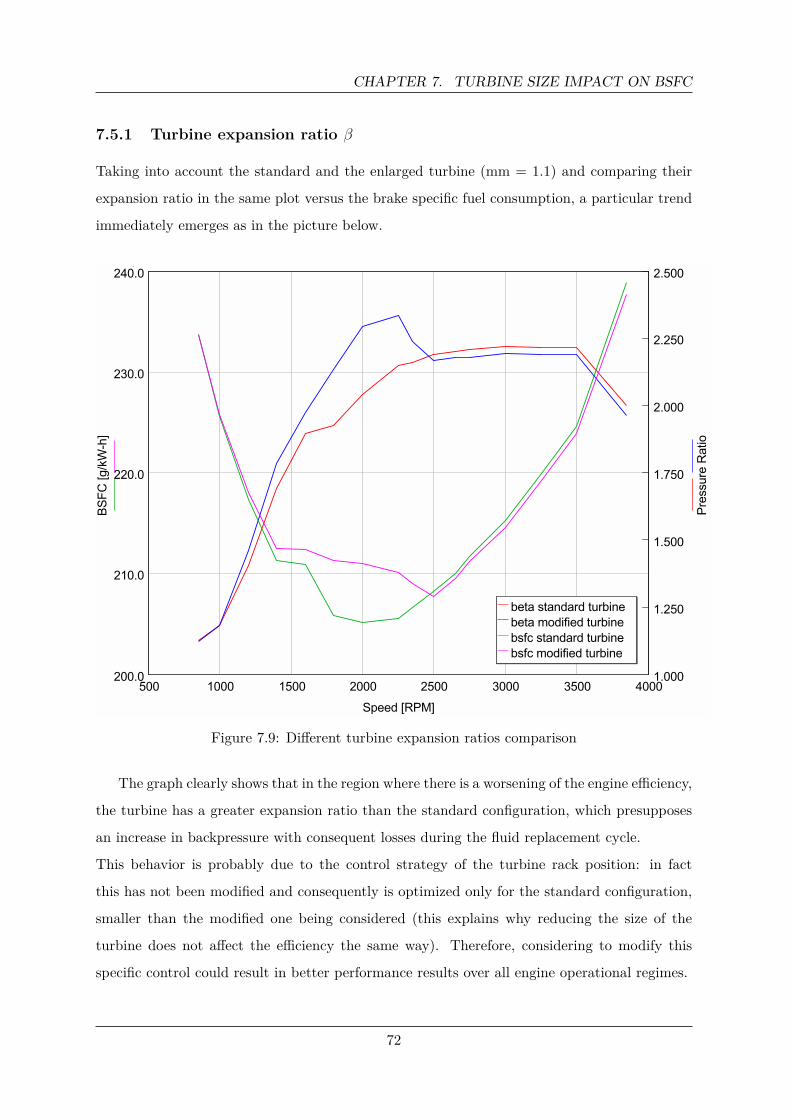
CHAPTER 7. TURBINE SIZE IMPACT ON BSFC
7.5.1 Turbine expansion ratio β
Taking into account the standard and the enlarged turbine (mm = 1.1) and comparing their
expansion ratio in the same plot versus the brake specific fuel consumption, a particular trend
immediately emerges as in the picture below.
Figure 7.9: Different turbine expansion ratios comparison
The graph clearly shows that in the region where there is a worsening of the engine efficiency,
the turbine has a greater expansion ratio than the standard configuration, which presupposes
an increase in backpressure with consequent losses during the fluid replacement cycle.
This behavior is probably due to the control strategy of the turbine rack position: in fact
this has not been modified and consequently is optimized only for the standard configuration,
smaller than the modified one being considered (this explains why reducing the size of the
turbine does not affect the efficiency the same way). Therefore, considering to modify this
specific control could result in better performance results over all engine operational regimes.
72
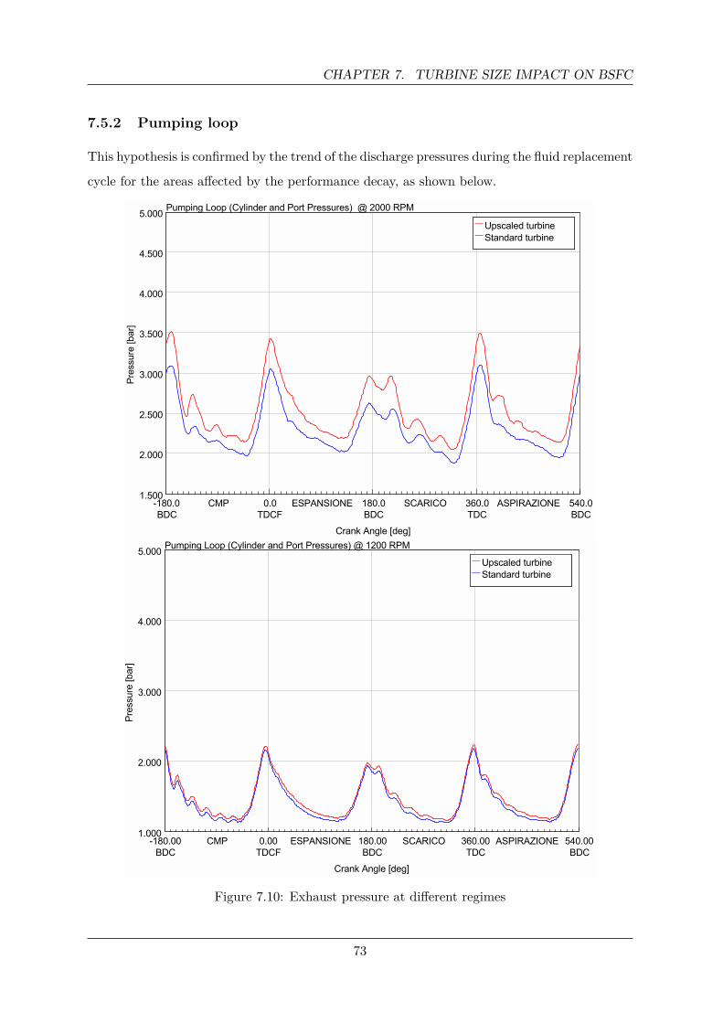
CHAPTER 7. TURBINE SIZE IMPACT ON BSFC
7.5.2 Pumping loop
This hypothesis is confirmed by the trend of the discharge pressures during the fluid replacement
cycle for the areas affected by the performance decay, as shown below.
Figure 7.10: Exhaust pressure at different regimes
73

CHAPTER 7. TURBINE SIZE IMPACT ON BSFC
7.6 Control strategy
The combustion process is very complex and it takes place through a series of steps that lead
to the generation of torque. In particular for diesel engines, after the mixture has been injected
into the combustion chamber and the ignition delay τi has elapsed (which does not scale with
the rotational speed of the engine) the premixed combustion phase starts. This translates
into a sharp increase of pressure inside the chamber with a peak in terms of heat release rate
HRR, consequent fatigue stresses on the engine parts and loud noise typical of these engines.
Thanks to new technologies, such as the use of the common rail, which allows to use higher
injection pressures (up to 2000 bar), it has been possible to contain and improve some of these
parameters but a compromise needs to be found.
In accordance with traditional literature the combustion process should have an appropriate
timing in order to extract the maximum potential from the fuel and reach high performance.
One of the parameters used to obtain this specific phasing is the MFB which stands for Mass
Fraction Burned. Best results are obtained for MFB50, meaning the 50% of mass burned,
situated around 10 ATDC (After Top Dead Center). An example of pressure and MFB trends
are shown in the picture below.
Figure 7.11: Pressure and MFB trends
After injection starts, there’s an initial delay and then the mass fraction burned increases with
a cubic trend, usually reaching reaching its completion after 40/50 ATDC.
74
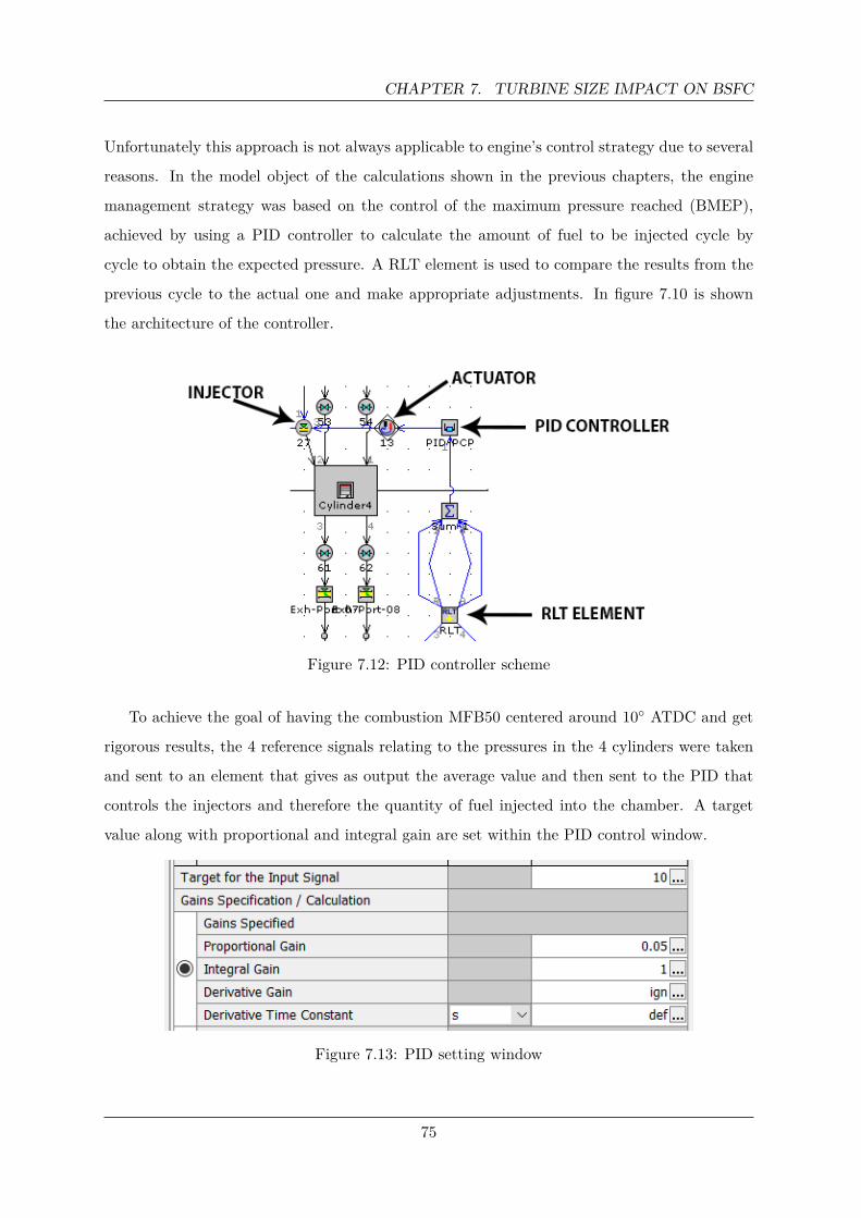
CHAPTER 7. TURBINE SIZE IMPACT ON BSFC
Unfortunately this approach is not always applicable to engine’s control strategy due to several
reasons. In the model object of the calculations shown in the previous chapters, the engine
management strategy was based on the control of the maximum pressure reached (BMEP),
achieved by using a PID controller to calculate the amount of fuel to be injected cycle by
cycle to obtain the expected pressure. A RLT element is used to compare the results from the
previous cycle to the actual one and make appropriate adjustments. In figure 7.10 is shown
the architecture of the controller.
Figure 7.12: PID controller scheme
To achieve the goal of having the combustion MFB50 centered around 10 ATDC and get
rigorous results, the 4 reference signals relating to the pressures in the 4 cylinders were taken
and sent to an element that gives as output the average value and then sent to the PID that
controls the injectors and therefore the quantity of fuel injected into the chamber. A target
value along with proportional and integral gain are set within the PID control window.
Figure 7.13: PID setting window
75
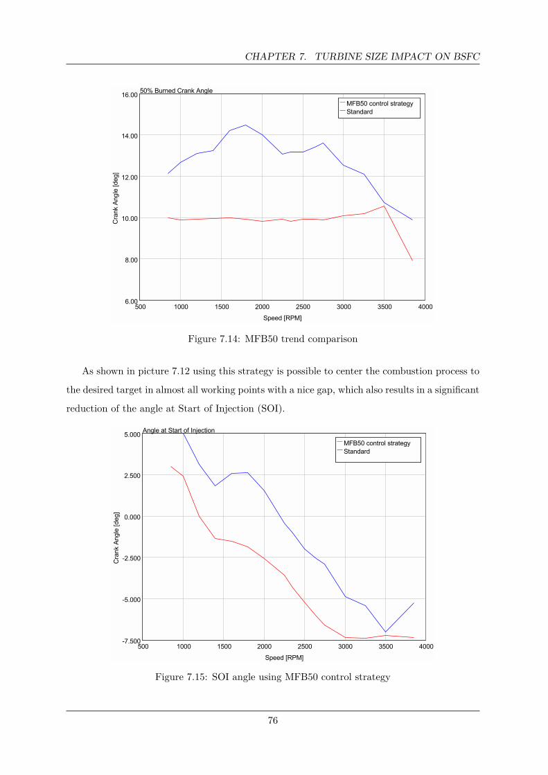
CHAPTER 7. TURBINE SIZE IMPACT ON BSFC
Figure 7.14: MFB50 trend comparison
As shown in picture 7.12 using this strategy is possible to center the combustion process to
the desired target in almost all working points with a nice gap, which also results in a significant
reduction of the angle at Start of Injection (SOI).
Figure 7.15: SOI angle using MFB50 control strategy
76
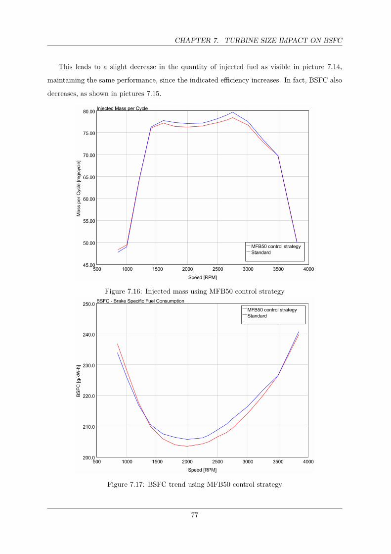
CHAPTER 7. TURBINE SIZE IMPACT ON BSFC
This leads to a slight decrease in the quantity of injected fuel as visible in picture 7.14,
maintaining the same performance, since the indicated efficiency increases. In fact, BSFC also
decreases, as shown in pictures 7.15.
Figure 7.16: Injected mass using MFB50 control strategy
Figure 7.17: BSFC trend using MFB50 control strategy
77
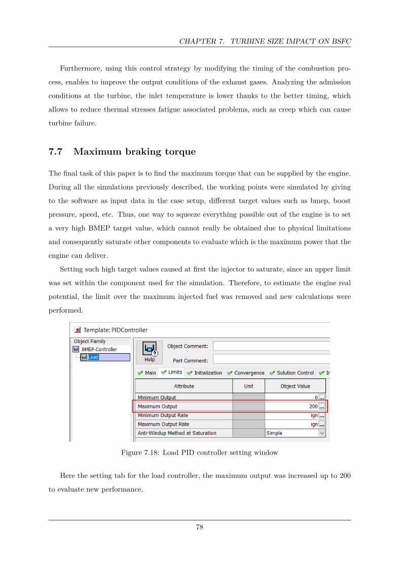
CHAPTER 7. TURBINE SIZE IMPACT ON BSFC
Furthermore, using this control strategy by modifying the timing of the combustion pro-
cess, enables to improve the output conditions of the exhaust gases. Analyzing the admission
conditions at the turbine, the inlet temperature is lower thanks to the better timing, which
allows to reduce thermal stresses fatigue associated problems, such as creep which can cause
turbine failure.
7.7 Maximum braking torque
The final task of this paper is to find the maximum torque that can be supplied by the engine.
During all the simulations previously described, the working points were simulated by giving
to the software as input data in the case setup, different target values such as bmep, boost
pressure, speed, etc. Thus, one way to squeeze everything possible out of the engine is to set
a very high BMEP target value, which cannot really be obtained due to physical limitations
and consequently saturate other components to evaluate which is the maximum power that the
engine can deliver.
Setting such high target values caused at first the injector to saturate, since an upper limit
was set within the component used for the simulation. Therefore, to estimate the engine real
potential, the limit over the maximum injected fuel was removed and new calculations were
performed.
Figure 7.18: Load PID controller setting window
Here the setting tab for the load controller, the maximum output was increased up to 200
to evaluate new performance.
78
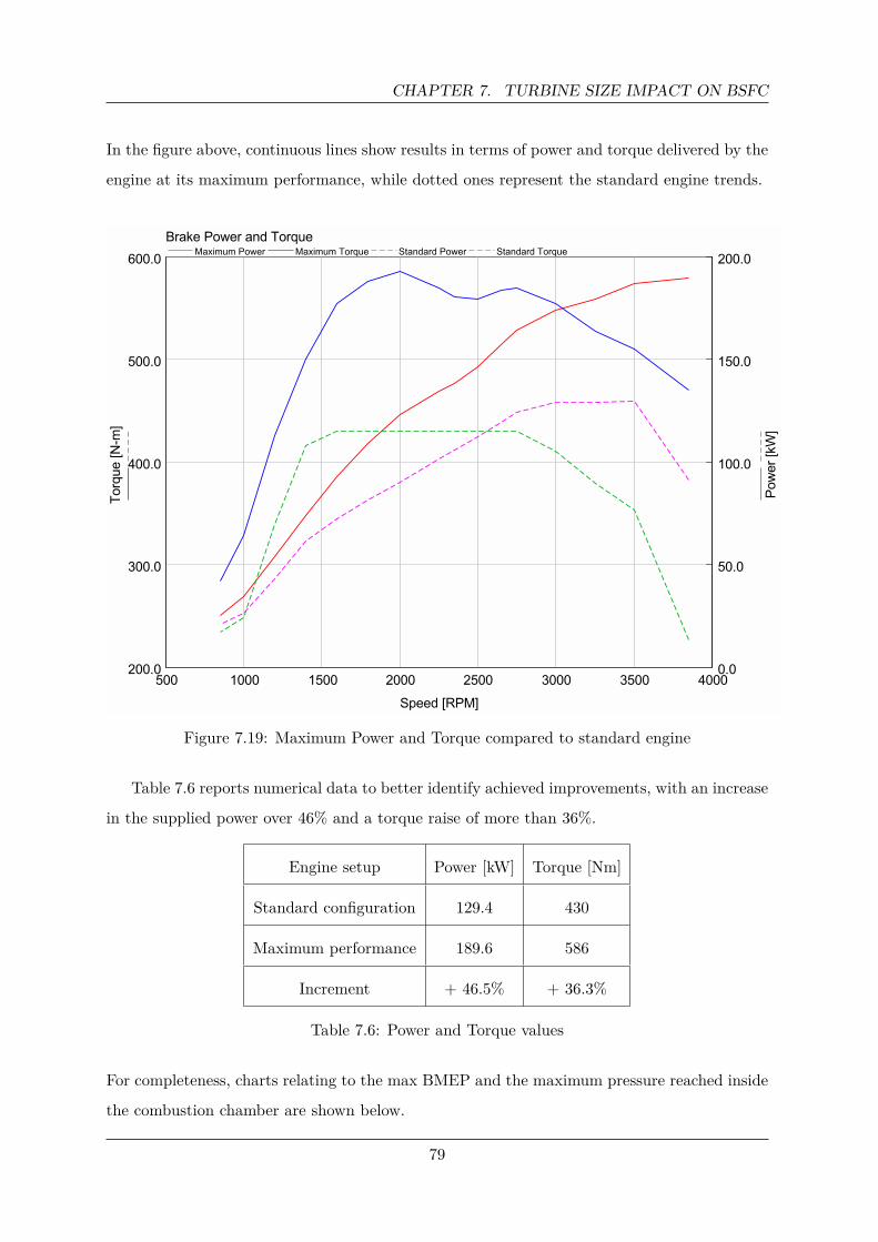
CHAPTER 7. TURBINE SIZE IMPACT ON BSFC
In the figure above, continuous lines show results in terms of power and torque delivered by the
engine at its maximum performance, while dotted ones represent the standard engine trends.
Figure 7.19: Maximum Power and Torque compared to standard engine
Table 7.6 reports numerical data to better identify achieved improvements, with an increase
in the supplied power over 46% and a torque raise of more than 36%.
Engine setup Power [kW] Torque [Nm]
Standard configuration 129.4 430
Maximum performance 189.6 586
Increment + 46.5% + 36.3%
Table 7.6: Power and Torque values
For completeness, charts relating to the max BMEP and the maximum pressure reached inside
the combustion chamber are shown below.
79
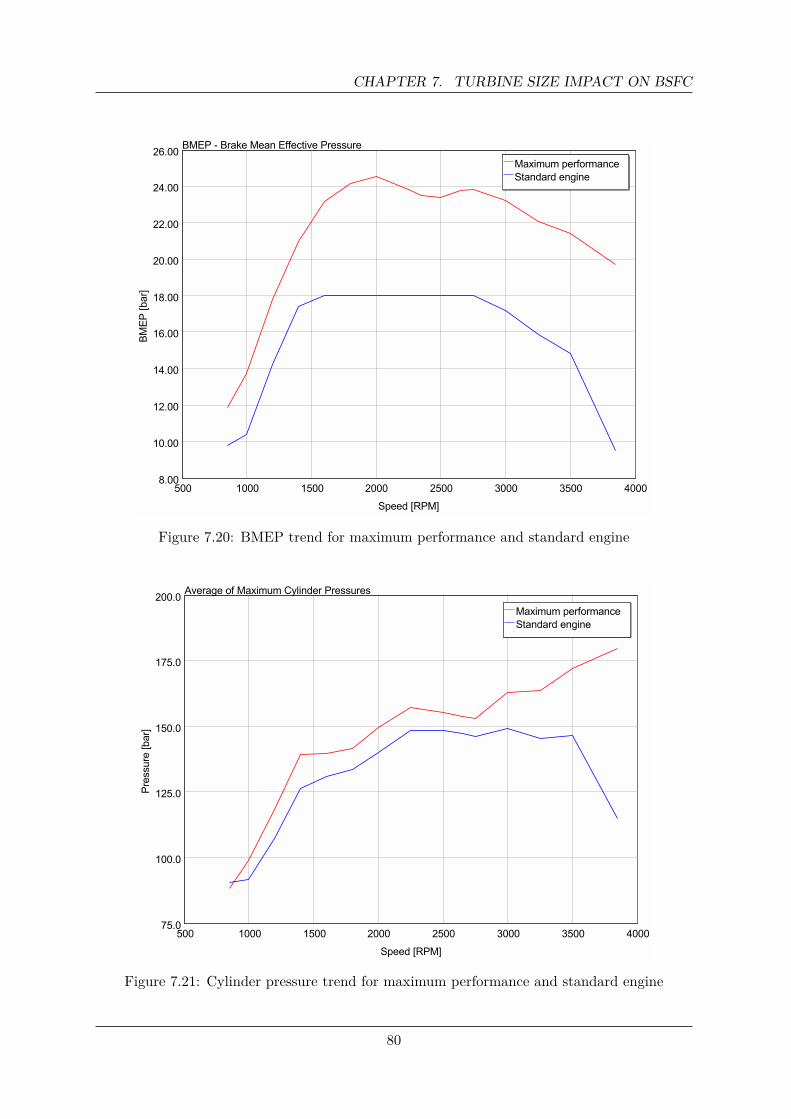
CHAPTER 7. TURBINE SIZE IMPACT ON BSFC
Figure 7.20: BMEP trend for maximum performance and standard engine
Figure 7.21: Cylinder pressure trend for maximum performance and standard engine
80
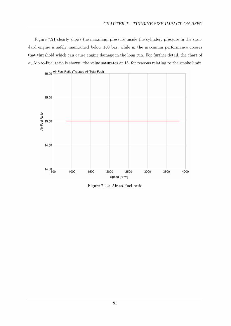
CHAPTER 7. TURBINE SIZE IMPACT ON BSFC
Figure 7.21 clearly shows the maximum pressure inside the cylinder: pressure in the stan-
dard engine is safely maintained below 150 bar, while in the maximum performance crosses
that threshold which can cause engine damage in the long run. For further detail, the chart of
α, Air-to-Fuel ratio is shown: the value saturates at 15, for reasons relating to the smoke limit.
Figure 7.22: Air-to-Fuel ratio
81
Chapter 8
Conclusions
The objective of the thesis was to develop and validate the methodology that could be used for
radial turbine geometrical parameters optimization based on CFD analysis and application to
engine performance assessment. The software used in the first part of the simulation, provides
good results in different working conditions, even with poorly refined mesh parameters. To
create a high quality mesh more calculation power is definitely needed, especially when the
geometry gets more complex or if the complete stage of the turbine (including impeller) is
considered. In general, the methods developed and the gas implementation have shown good
results for this turbine. If no further data are available, the properties of air can be used for
diesel exhaust gas calculations. The error associated with neglecting the combustion products
is usually no more than about 2%. In a more rigorous approach, corrections must be taken
into account for the actual exhaust gas composition (increased H2O and CO2, decreased O2).
An additional difficulty with this approach is the necessity to consider the variable exhaust
gas composition, which changes with the engine load factor and the air-to-fuel ratio. Anyways,
this specific turbine geometry performs very well under steady-state flow condition, especially
for low loads. Losses are limited and the volute manages to develop the fluid by converting
the exhaust pressure into kinetic energy to spin the impeller and generate power. Relating to
this part, the analysis could be further developed with greater computational power to solve
rotating mesh problems, and by performing experimental tests to get practical feedback.
As regards the second part of the thesis, an ad-hoc software was used to carry out the
simulations and evaluate the impact of different turbine geometries on the engine performance,
using as well data from the 3D model. The standard geometry configuration allows good
performance to be obtained for most of the simulated operating points, with slight losses in
82
CHAPTER 8. CONCLUSIONS
terms of efficiency at high regimes. The changes made to the geometry refer to variations in the
turbine A/R ratio, by modifying turbine’s housing size. Results shown that the reduction of
turbine size improves performance (in terms of BSFC) in the region of low loads at the expense
of a deterioration that is obtained at higher loads mainly due to the increased backpressure
and pumping loss. Respectively, a larger turbine leads to slight improvements in the area of
high loads but much more substantial losses in the medium range, explainable considering the
higher expansion ratio of the turbine caused by the rack control strategy which is optimized
for the standard turbine rather than the modified one.
It should be noted that, turbine’s size variations were made using a specific software pa-
rameter called ”mass multiplier”, which easily allows to switch from a configuration to another.
This was done after making sure that the method won’t affect significantly the results of simu-
lation by comparing the scaling method of the software with a reliable method developed after
experimental tests.
8.1 Future work
The geometrical design the volute can be further improved by modelling the inlet duct of the
volute for a more detailed representation of the turbine.
In terms of CFD simulation, a major step that can be done is the complete study of the
turbine including the impeller. That will allow to analyze and study the actual expansion ratio
of the turbine and if necessary act on it in order to improve its performance to exploit as much
as possible the energy of the exhaust gases. Changing the type of approach to simulation, taking
advantage of the data obtained to modify the 3D model of the impeller: the number of blades,
the angle and their geometry itself. As previously described, this requires a greater computing
power, a greater number of experimental data as well as better knowledge of the entire system.
As a further step forward, the study of the entire turbocharger could be performed, by means
of simulating both the compressor and the turbine stages together and matching the results to
evaluate the real performance of the product and evaluating the response of the compressor.
Regarding GT-Power side, further analysis may be carried out, by means of considering
different engine parameters which could be affected by turbocharger variations and their impact
on performance.
83
CHAPTER 8. CONCLUSIONS
8.2 Contribution
The thesis work was carried out in close cooperation with the help of dr. inz. Dmytro
Samoilenko, in the Erasmus+ Exchange Programme at the Politechnika Warszawska, WUT
(Warsaw University of Technology) and completed at the Politecnico di Torino under the su-
pervision of prof. ing. Mirko Baratta. A big thanks goes to them for following and supporting
me during this journey.
A special thanks goes to Vittoria, Federico, Marco, Michele and Giovanni for the help and
support they gave me during all these years and to Valerio and Giovanni for sustaining me
during the last period of my studies.
Finally, my deep and sincere gratitude goes to my father, mother and sister for their continu-
ous help, encouragement, spiritual and economic support. This journey would not have been
possible if not for them, and I dedicate this milestone to them.
84
Bibliography
[1] H. K. Versteeg, W. Malalasekera, An Introduction to Computational Fluid Dy-
namics, 2nd Edition, Pearson Education Limited, Edinburgh Gate, Harlow, 2007.
[2] R. Kabral, M. Abom, Investigation of flow-acoustic interaction in automotive tur-
bocharger, KTH Royal Institute of Technology, Sweden, 2014.
[3] BorgWarner Turbo Systems, Performance catalogue, Volume 5, 2018.
[4] Melett, Wabtec Corporation, www.melett.it/technical/types-of-turbocharger.
[5] Baines, N. C., Fundamentals of Turbocharging Concepts NREC, White River
Junction, Vermont, 2005.
[6] S. Nguyen, Thermodynamics of Turbochargers, Springer, Germany, 2014.
[7] H. Moustaphe, M. Zelesky, N. Baines, D. Japikse, Axial and Radial Turbines,
Concepts NREC, White River Junction, Vermont, 2003.
[8] SOLIDWORKS, Flow Simulation Technical Reference, Dassault Systemes, 2017.
[9] GT-Power suite website, www.gtisoft.com/gt-suite-applications/propulsion-
systems/gt-power-engine-simulation-software.
[10] Honeywell Garrett, Original performance, Volume 7, USA, 2015.
[11] N. Mastorakis, V. Mladenov, Computational Problems in Engineering, Springer,
Volume 307 Switzerland, 2014.
[12] C. Bell, D. Zimmerle, T. Bradley, D. Olsen, P. Young, ”Scalable turbocharger
performance maps for dynamic state-based engine models”, 2016.
[13] GT-SUITE, Flow Theory Manual, Gamma Technologies, 2014.
85

BIBLIOGRAPHY
[14] Audi SQ7 TDI V8 TDI with electric powered compressor and 48 volt electrical
subsystem, Audi Technology Portal, 3/2016.
86
Related Documents