Wealth Creation, Wealth Dilution and Population Dynamics Christa N. Brunnschweiler ! , University of East Anglia Pietro F. Peretto y , Duke University Simone Valente z , University of East Anglia October 18, 2017 Abstract Wealth creation driven by R&D investment and wealth dilution caused by discon- nected generations interact with householdsí fertility decisions, delivering a theory of sustained endogenous output growth with a constant endogenous population level in the long run. Unlike traditional theories, our model fully abstracts from Malthusian mechanisms and provides a demography-based view of the long run where the ratios of key macroeconomic variables ñ consumption, labor incomes and Önancial assets ñ are determined by demography and preferences, not by technology. Calibrating the model parameters on OECD data, we show that negative demographic shocks induced by barriers to immigration or increased reproduction costs may raise growth in the very long run, but reduce the welfare of a long sequence of generations by causing perma- nent reductions in the mass of Örms and in labor income shares, as well as prolonged stagnation during the transition. JEL Codes: O41, J11, E25 Keywords: R&D-based growth, Overlapping generations, Endogenous fertility, Population level, Wealth dilution. ! Christa N. Brunnschweiler, School of Economics, University of East Anglia, NR4 7TJ Norwich, United Kingdom. E-mail: [email protected]. y Pietro F. Peretto, Department of Economics, Duke University, Durham, NC 27708. Phone: (919) 660- 1807 Fax: (919) 684-8974. E-mail: [email protected] z Simone Valente, School of Economics, University of East Anglia, NR4 7TJ Norwich, United Kingdom. E-mail: [email protected]. 1

Welcome message from author
This document is posted to help you gain knowledge. Please leave a comment to let me know what you think about it! Share it to your friends and learn new things together.
Transcript

Wealth Creation, Wealth Dilution
and Population Dynamics
Christa N. Brunnschweiler!, University of East Anglia
Pietro F. Perettoy, Duke University
Simone Valentez, University of East Anglia
October 18, 2017
Abstract
Wealth creation driven by R&D investment and wealth dilution caused by discon-
nected generations interact with householdsí fertility decisions, delivering a theory of
sustained endogenous output growth with a constant endogenous population level in
the long run. Unlike traditional theories, our model fully abstracts from Malthusian
mechanisms and provides a demography-based view of the long run where the ratios
of key macroeconomic variables ñ consumption, labor incomes and Önancial assets ñ
are determined by demography and preferences, not by technology. Calibrating the
model parameters on OECD data, we show that negative demographic shocks induced
by barriers to immigration or increased reproduction costs may raise growth in the very
long run, but reduce the welfare of a long sequence of generations by causing perma-
nent reductions in the mass of Örms and in labor income shares, as well as prolonged
stagnation during the transition.
JEL Codes: O41, J11, E25
Keywords: R&D-based growth, Overlapping generations, Endogenous fertility,
Population level, Wealth dilution.
!Christa N. Brunnschweiler, School of Economics, University of East Anglia, NR4 7TJ Norwich, United
Kingdom. E-mail: [email protected] F. Peretto, Department of Economics, Duke University, Durham, NC 27708. Phone: (919) 660-
1807 Fax: (919) 684-8974. E-mail: [email protected] Valente, School of Economics, University of East Anglia, NR4 7TJ Norwich, United Kingdom.
E-mail: [email protected].
1
1 Introduction
Is demography destiny? How economic development interacts with population dynamics
is a key question that has gained renewed interest in the profession: demographic change
lies at the origin of many challenges faced by modern societies, and the widespread decline
of fertility rates in the industrialized world a§ects policymaking on a global scale. In
the economics literature, there is an established body of theories that endogeneize private
fertility choices and their response to economic growth (Bloom et al. 2013). Yet, the
majority of these models ñ with exceptions that we discuss below ñ predict that the economy
converges to long-run equilibria where population grows exponentially at a constant rate,
which is at odds with the demographers view of the long run (Wrigley, 1988). In this
paper, we propose a model where the interaction between individual fertility choices and
productivity growth led by innovations delivers a theory of the population level: in the long
run, output grows at a positive endogenous rate, while the mass of population achieves a
constant endogenous level. The nature of this steady state, and the determinants of long-run
consumption and income shares are in stark contrast with the conclusions of the existing
literature.
The two building blocks of our model are the overlapping-generations demographic struc-
ture and the Schumpeterian theory of R&D-based endogenous growth. In the demographic
block of the model, we assume that households optimize lifetime consumption facing a pos-
itive probability of death (Yaari, 1965; Blanchard, 1985), and we extend this framework to
endogeneize fertility: households choose the number of children by maximizing own util-
ity subject to a pure time cost of reproduction. The demographic structure implies that
per capita consumption growth is limited by Önancial wealth dilution: since disconnected
generations optimize over Önite horizons, each new cohort entering the economy captures a
fraction of the existing wealth by pursuing independent accumulation decisions that reduce
the consumption possibilities of all generations.1 The novel insight of our model is that
wealth dilution interacts with fertility choices and is thus both a consequence and a deter-
minant of population dynamics. SpeciÖcally, Önancial wealth dilution tends to reduce the
economyís fertility rate by limiting consumption expenditures. The key question is whether
this negative partial-equilibrium e§ect translates into a general-equilibrium negative feed-
1Buiter (1988) and Weil (1989) provide an early recognition of the wealth dilution e§ect in the Blanchard-
Yaari framework with exogenous population growth.
1

back of population on fertility. The answer hinges on how the supply side generates growth
in Önancial assets, and more precisely, on how population a§ects the economyís rate of
wealth creation.
We model the production side of the economy as an R&D-based model of endogenous
growth where assets represent ownership of Örms. The key characteristic of the process of
wealth creation is that both the mass of Örms and the average proÖtability of each Örm grow
endogenously as a result of di§erent R&D activities (Peretto, 1998; Peretto and Connolly,
2007). Growth in the total value of Örms results from both vertical innovations (i.e., each
individual Örm invests in R&D that raises internal productivity) and horizontal innovations
(i.e., new Örms enter the market) that compete for labor as an input. In equilibrium, the
ratio between the market wage rate and assets per capita is increasing in population size.
This relationship propagates the e§ect of wealth dilution, giving rise to a negative feedback
of population on fertility that eventually brings population growth to a halt in the long
run. Hence, unlike standard growth models predicting exponential population growth,2 we
obtain a theory of the population level where net fertility is asymptotically zero despite a
positive endogenous rate of output growth.
Our results di§er from those of the existing literature in two major ways. First, with
respect to alternative models admitting a constant endogenous population level in the long
run, our distinctive hypothesis is that production possibilities are not constrained by re-
source scarcity. To the best of our knowledge, all the existing theories of the population
level hinge on Malthusian mechanisms whereby population is bounded by the scarcity of
essential factors available in Öxed supply. Malthusian mechanisms may take various forms:
decreasing returns to scale in Eckstein et al. (1988), land scarcity combined with subsis-
tence requirements in Galor and Weil (2000), open-access livestock in Brander and Taylor
(1998). Two borderline cases are Strulik and Weisdorf (2008) and Peretto and Valente
(2015), where the Öxed factor is a marketed input and its relative scarcity creates price
e§ects that tend to reduce fertility through increased cost of living and/or reduced real
incomes.3 Our present analysis, instead, fully abstracts from Malthusian mechansism by
2The class of growth models with endogenous fertility predicting exponential population growth is quite
large (see Ehrlich and Lui, 1997) and encompasses all the well-established speciÖcations of the supply side,
from neoclassical technologies (e.g., Barro and Becker, 1989) to endogenous growth frameworks (e.g., Chu
et al. 2013).3 In Strulik and Weisdorf (2008), scarcity increases the relative price of food and thereby the private
2

ruling out Öxed endowments: the predicted fertility decline originates in the dilution of
Önancial wealth. Moreover, we abstract from the research questions typically tackled by
Malthusian models ñ prominently, the rise of and escape from pre-industrial stagnation
traps ñ to address inherently forward-looking issues.
The second main di§erence with respect to the existing literature is the determination
of key macroeconomic variables in the long run. In the steady state of our model, the
ratios of aggregate consumption and of total labor incomes to aggregate Önancial wealth
are exclusively determined by demography and preference parameters. This is in stark
contrast with traditional balanced-growth models ñ especially those assuming a neoclassical
supply-side structure ñ where the same ëlong-run ratiosí are fundamentally determined by
technology. A major implication of our result is that exogenous shocks hitting demographic
or preference parameters ñ and by extension, public policies a§ecting reproduction costs,
life expectancy, or migration ñ have a Örst-order impact on income shares, growth and
welfare. We perform a quantitative analysis of the model that delivers further insights in
this respect. We calibrate the model parameters using data for OECD countries, and we
assess the impact of exogenous demographic shocks on consumption, growth, and welfare
using numerical simulations. Negative demographic shocks caused by higher reproduction
costs and immigration barriers induce permanent reductions in labor income shares while
having a ëreversed impactí on growth rates: growth may be higher in the very long run, but
it is lower during the transition. This phenomenon originates in the positive co-movement
between population and mass of Örms, and bears substantial consequences for welfare.
Using a cohort-speciÖc index of lifetime utility, we show that a permanent shock reducing
net immigration by 25% reduces welfare for all the generations entering the economy up to
eighty years after the shock, due to the combined e§ects of permanently lower labor incomes
and stagnating transitional growth.
The paper is organized as follows. After describing the demographic model (section 2)
and the production side of the economy (section 3), we characterize the steady state with
constant population in section 4. Section 5 derives key analytical results and extends the
model to include migration. Section 6 presents our quantitative analysis, and Section 7
cost of reproduction resulting in fertility decline. In Peretto and Valente (2015), growing rents from scarce
natural resources a§ect fertility via income e§ects that, assuming substitutability between land and labor
inputs in production, give rise to a stationary population level that is nonetheless determined by resource
scarcity via resource prices.
3
concludes. To preserve expositional clarity, we report detailed derivations and proofs in a
separate Appendix.
2 The Demographic Model
The economy is populated by overlapping generations of single-individual families facing a
constant probability of death (Yaari, 1965; Blanchard, 1985). We extend the Blanchard-
Yaari structure by assuming that fertility is endogenously determined by private beneÖts
and costs: each household derives utility from the mass of children it rears subject to a pure
time cost of reproduction. Since wealth is not transmitted in a dynastic fashion, the arrival
of new individuals dilutes Önancial wealth per capita, a§ecting consumption possibilities as
well as population dynamics via fertility choices.
2.1 Households
The economyís population consists of di§erent cohorts of single-individual families indexed
by their birth date j. Individual variables take the form xj (t), where j 2 ("1; t) is the
cohort index and t 2 ("1;1) is continuous calendar time.4 In particular, cj (t) denotes
consumption at time t of an individual born at time j < t, and bj (t) denotes the mass of
children reared at time t by an agent who belongs to cohort j. The expected lifetime utility
of an individual born at time j is
UEj =
Z 1
j[ln cj (t) + ln bj (t)] e
%(#+$)(t%j)dt; (1)
where > 0 is the weight attached to the utility from rearing bj (t) children, - > 0 is the rate
of time preference, and . > 0 is the constant instantaneous probability of death. Di§erently
from dynastic models with pure altruism (e.g., Becker and Barro, 1988), individuals do
not maximize their descendantsí utility via intergenerational transfers. Children leave the
family immediately after birth, enter the economy as workers owning zero assets, and make
plans independently from their predecessors. Individuals accumulate assets and allocate one
unit of time between working and child-rearing activities. The individual budget constraint
is
_aj (t) = (r (t) + .) aj (t) + (1" 1bj (t))w (t)" p (t) cj (t) ; (2)
4Using standard notation, the time-derivative of variable xj (t) is _xj (t) !dxj (t) =dt.
4
where aj is individual asset holdings, r is the rate of return on assets, w is the wage rate, p
is the price of the consumption good, and 1 > 0 is the time cost of child rearing per child.
The term (1" 1b) thus represents individual labor supply.
An individual born at time j maximizes (1) subject to (2), taking the paths of all prices
as given. Necessary conditions for utility maximization are the individual Euler equation
for consumption_cj (t)
cj (t)+_p (t)
p (t)= r (t)" -; (3)
and the condition equating the marginal rate of substitution between consumption and
child-rearing to the ratio of the respective marginal costs,
1=cj (t)
=bj (t)=
p (t)
1w (t); or bj (t) =
1$p (t) cj (t)
w (t); (4)
where 1w is the private opportunity cost of reproduction in terms of foregone labor income.
The second expression in (4) emphasizes that individual fertility is proportional to the ratio
between consumption expenditure and the market wage rate in each instant, a result that
will play an important role in our analysis.
2.2 Aggregation and Population Dynamics
Denoting by kj (t) the size of cohort j at time t, adult population L (t) and total births
B (t) equal
L (t) %Z t
%1kj (t) dj and B (t) %
Z t
%1kj (t) bj (t) dj:
Similarly, total assets A (t) and aggregate consumption C (t) equal
A (t) %Z t
%1kj (t) aj (t) dj and C (t) %
Z t
%1kj (t) cj (t) dj:
Following the tradition of the literature, we deÖne per capita variables by referring to
adult population L (t) as to the economyís population: births, assets, and consumption per
capita are respectively denoted by b % B=L, a % A=L, and c % C=L.5 Since individuals
are homogeneous within cohorts, the size of each cohort declines over time at rate ., which
5The caveat in order is that population is in fact L+B, so that variables per capita should in principle
be deÖned as the aggregate variables divided by L + B. Doing so would complicate the algebra without
changing the results.
5

therefore represents the economyís mortality rate. Population evolves according to the
demographic law
_L (t) = B (t)" .L (t) : (5)
Total births are determined by householdsí reproduction choices: aggregating the individual
fertility decision (4) across cohorts, we have
B (t) =
1$p (t)
R t%1 kj (t) cj (t) dj
w (t)=
1$p (t)C (t)
w (t): (6)
Result (6) is a static equilibrium relationship between the economyís gross fertility, con-
sumption expenditure and wages. Fertility and consumption dynamics will be subject to
the wealth constraint: aggregation of the individual budget (2) across cohorts yields the
growth rate of total assets
_A (t)
A (t)= r (t) +
w (t) (L (t)" 1B (t))A (t)
"p (t)C (t)
A (t); (7)
where the term L"1B equals aggregate net labor supply and captures the negative impact
of reproduction costs on the pace of accumulation.
2.3 Consumption and Wealth Dilution
We characterize individual consumption by exploiting the standard deÖnition of human
wealth,
h (t) %Z 1
tw (s) $ e%
R st (r(v)+$)dvds: (8)
Combining the fertility equation (4) with the budget constraint (2), we obtain the individual
expenditure of an agent born at time j,
p (t) cj (t) =-+ .
1 + $ [aj (t) + h (t)] : (9)
Expression (9) shows that individual expenditure is proportional to individual wealth, given
by the sum of current Önancial and human wealth. Financial wealth aj is cohort-speciÖc
whereas human wealth h only depends on the anticipated paths of the wage and the interest
rates. The existence of a preference for children, , reduces the individual propensity to
consume out of wealth. Integrating individual expenditures across cohorts and dividing by
the population level, we can write per capita consumption expenditure as
p (t) c (t) =-+ .
1 + $ [a (t) + h (t)] : (10)
6
Despite their apparent similarity, expressions (9) and (10) represent di§erent objects. In
the individual expenditure function, both cj (t) and aj (t) are optimized values chosen by
individuals (given the initial assets aj (j) = 0). The per capita variables c (t) and a (t) are,
instead, average values a§ected by the age structure of the population. This distinction
turns out to be relevant when computing growth rates. Time-di§erentiation of (10) yields
_c (t)
c (t)+_p (t)
p (t)= r (t)" -"
(-+ .)
1 (1 + )$a (t)
w (t)| {z }Financial wealth dilution
: (11)
Comparing this expression to the individual Euler equation (3), we observe that the growth
rates of per capita and individual consumption expenditure di§er by the last term in (11),
which represents the rate of Önancial wealth dilution induced by fertility ñ i.e., the share
of per capita wealth that the members of each new cohort capture upon their arrival: from
(10) and (6), we have
(-+ .)
1 (1 + )$a (t)
w (t)| {z }Financial wealth dilution
=A (t) =L (t)
h (t) +A (t) =L (t)$B (t)
L (t): (12)
Financial wealth dilution a§ects per capita consumption growth because generations are dis-
connected. Since wealth is not redistributed in a dynastic fashion through intergenerational
transfers, new cohorts enter the economy with zero assets and start pursuing their own ac-
cumulation and fertility plans independently from their predecessors. We might label this
phenomenon as passive wealth dilution, in the sense that the consumption possibilities of
each generation are subject to the accumulation and fertility decisions of all the subsequent
generations. In fact, passive wealth dilution does not arise in models with pure altruism
where the head of the dynasty optimizes the use of all private assets over an inÖnite time
horizon, and the last term in (11) disappears. While these general characteristics of the
wealth dilution mechanism have long been recognized in the literature ñ see the early con-
tributions by Buiter (1988) and Weil (1989) ñ our analysis will add an important insight. In
the present model, Önancial wealth dilution interacts with fertility choices and is thus both
a consequence and a determinant of population dynamics. More precisely, Önancial wealth
dilution tends to reduce the economyís fertility rate by limiting consumption expenditure,
as we show next.
7

2.4 Fertility dynamics: expenditure and wage channels
To gain insight into population-fertility interactions, consider how the fertility rate b would
respond to a change in population L for given levels of aggregate Önancial wealth A and
individual human wealth h. From (6) and (10), the fertility rate equals
b (t) =
1
Expenditure channelz }| {p (t) c (t)
w (t)|{z}Wage channel
=
1
-+ .
1 +
'A (t)
L (t)+ h (t)
(1
w (t)(13)
The central term of (13) shows that for given levels of wealth, changes in population size
a§ect the fertility rate through two channels. The expenditure channel incorporates the
mechanism of wealth dilution discussed in the previous subsection: an increase in L for
given A reduces assets per capita a = A=L, and thereby consumption expenditure per
capita. Hence, a growing population tends to reduce fertility through the dilution of Önancial
wealth. The wage channel, instead, operates through the impact of population on the wage
that prevails on the labor market: population dynamics a§ecting the equilibrium wage rate
will also a§ect fertility by modifying the householdsí opportunity cost of reproduction.
The impact of population on fertility via the wage channel is generally ambiguous: its
sign and strength are determined on the supply side of the economy, which we have not
modeled yet. The key equation is the growth rate of the fertility rate: time-di§erentiating
(13), and substituting the Euler equation (11) for consumption growth along with the
dynamic wealth constraint (7) in per capita terms, we obtain
_b (t)
b (t)= b (t)
)1 + 1
1 +
$w (t)
a (t)
*" -" . "
w (t)
a (t)+_a (t)
a (t)"_w (t)
w (t)" (-+ .)
1 (1 + )$a (t)
w (t); (14)
where the last term is the rate of Önancial wealth dilution. Equation (14) delivers funda-
mental information because it incorporates the aggregation of all householdsí intertemporal
decisions concerning both fertility and consumption choices into a single expression that
only contains two variables, b and a=w, and their respective growth rates.6 Therefore,
by combining (14) with a model of the supply side determining the a=w ratio, we can
characterize the equilibrium dynamics of the economy as a reduced system in three ëcore
variablesí: population, fertility, and the asset-wage ratio. In this respect, we stress that
6The behavior of householdsí propensities to consume out of wealth is incorporated in (13) and, hence,
in (14).
8
di§erent speciÖcations of the supply side will deliver di§erent predictions. The following
taxonomy considers four general frameworks.
(i) Models without Önancial wealth. Suppose that Önancial assets do not exist because the
only accumulable factor of production is labor. In this setup, agents cannot pursue
consumption smoothing and equation (14) does not apply. Instead, the aggregate
wealth constraint (7) yields that per capita consumption expenditure is proportional
to the wage. From this follows immediately that the fertility rate, b, is constant and
generally di§erent from the death rate .. This result is independent of the speciÖcs
of production and complies with Lucasí (2002) observation that labor-land models
assuming a time-cost of reproduction typically predict that population grows expo-
nentially at a constant rate.7 For our purposes, the key point is that models without
Önancial assets remove wealth dilution from the analysis.
(ii) Neoclassical models with physical capital. In these models Önancial assets are claims
on physical capital and both labor and capital exhibit diminishing marginal returns
with constant returns to scale. For given aggregate capital, an increase in population
reduces capital per capita and thus has contrasting e§ects on the fertility rate: while
the equilibrium wage falls ñ reducing the opportunity cost of child rearing ñ wealth
dilution reduces consumption expenditure per capita. Most importantly, the endoge-
nous accumulation of capital brings the economy towards a constant capital-labor
ratio and, crucially, a constant asset-wage ratio a=w in the long run. From (14), this
implies that the fertility rate becomes constant and population grows exponentially
at a constant rate (proof in Appendix A). Hence, neoclassical models do not produce
a wealth dilution mechanism that is su¢ciently strong to stabilize the population.
(iii) Endogenous growth models with constant returns to capital. These models assume
constant returns to the accumulable factor but keep the assumption of decreasing
marginal returns to labor (e.g., Romer, 1986). Since the wage is inversely related
to the population level, the e§ects of a larger population for given wealth are sim-
ilar to those occurring in neoclassical models, but the implications for fertility are
7For example, assume that production combines labor with a Öxed input land. These speciÖcs yield
an equilibrium wage that is decreasing in population due to diminishing returns but does not produce a
feedback of population on fertility.
9
drastically di§erent due to the strong scale e§ect ñ the property that the return to
capital accumulation is increasing in population size. We characterize the dynamics
for this model in Appendix A. The main result is that the model produces either
explosive/degenerate paths, or a steady state with constant population and constant
endogenous growth of variables per capita. Such a steady state, however, admits pos-
itive output growth only under very restrictive conditions on parameters and, most
importantly, does not exist without assuming the strong scale e§ect.
(iv) Endogenous growth models with costly R&D. In R&D-based models of endogenous
growth, Önancial wealth A represents the aggregate value of Örms that raise pro-
ductivity by accumulating intangible assets such as knowledge and ideas. For our
purposes, we need to distinguish two sub-classes of models with radically di§erent
implications. The so called Örst-generation models (e.g., Romer, 1990; Aghion and
Howitt, 1992) exhibit the strong scale e§ect and behave very much like the AK model
discussed above. More interesting to us are the models with endogenous market struc-
ture (Peretto, 1998; Dinopoulos and Thompson, 1998, Howitt, 1999) that remove the
strong scale e§ect by combining in-house R&D with horizontal innovations that create
new Örms. In particular, when both types of R&D compete for labor as an input, the
wage response to increased population fully abstracts from neoclassical mechanisms
of diminishing returns (Peretto and Connolly, 2007). These properties o§er a radi-
cally di§erent theory of population dynamics because, contrary to what we observe
in frameworks (i)-(iii), the expenditure channel is fully operative and is neither o§set
nor dominated by a counteracting wage channel. We investigate this point in the
remainder of our analysis by modelling the supply side of the economy according to
Peretto and Connollyís (2007) speciÖcation.
The above considerations suggest two main remarks. First, frameworks (i)-(ii) neutral-
ize the role of wealth dilution as the potential source of negative feedbacks of population on
fertility and, more generally, exhibit a structural tendency to generate long-run equilibria
where the fertility rate is constant.8 The typical approach to rationalize declining and/or
8This is not a mere technical point: the economics literature on fertility makes extensive use of frameworks
(i)-(ii) to address research questions ñ i.e., the income-fertility relationship and the determinants of the
fertility decline ñ that ultimately require explaining how increases in the size of the population pull down
subsequent fertility rates.
10
constant population in these frameworks is to include Malthusian mechanisms that create
congestion in the use of essential natural resources and/or some form of quality-quantity
trade-o§ for children ñ a prominent example is Galor and Weil (2000). While this approach
is worthwhile and produces important insights, in this paper we deliberately take another
route by excluding Malthusian mechanisms from the analysis. The second remark is that
R&D-based models without scale e§ects can provide fundamentally di§erent insights on
population-fertility interactions because their core mechanism of wealth creation ñ i.e., the
accumulation of intangible assets raising the mass of Örms and each Örmís proÖtability ñ
propagates the wealth dilution mechanism and thereby gives rise to a general-equilibrium
negative feedback of population on fertility. We formally investigate this point in the next
two sections, obtaining a theory of the population level that fully abstracts from the Malthu-
sian mechanisms emphasized in the existing literature.
3 The Production Side
The economy produces the Önal consumption good by means of di§erentiatied intermedi-
ates produced by monopolistic Örms. Productivity growth is driven by both vertical and
horizontal innovations in the intermediate sector: incumbents pursue vertical R&D to raise
internal productivity, while outside entrepreneurs create new Örms to enter the market. The
model speciÖcs draw on Peretto and Connolly (2007), which yields a transparent derivation
of the equilibrium relationships linking the total value of Örms to population size and to
the market wage rate.
3.1 Final Sector
A competitive sector produces the Önal consumption good by assembling di§erentiated
intermediate products according to the technology
C (t) = N (t))%$$$1 $
Z N(t)
0xi (t)
$$1$ di
! $$$1
; (15)
where N is mass of intermediates, xi is the quantity of the i-th intermediate good, ? > 1
is the elasticity of substitution between pairs of intermediates, and @ > 1 is the degree of
increasing returns to specialization. Final producers take all prices and the mass of goods
11

as given, and demand intermediate goods according to the proÖt-maximizing condition
pxi (t) =p (t)C (t)
R N(t)0 xi (t)
$$1$ di
$ xi (t)%1$ (16)
where pxi is the price of intermediate good i.
3.2 Intermediate Producers: Incumbents
The typical intermediate Örm produces according to the technology
xi (t) = zi (t)- $ (`xi (t)" ') ; (17)
where zi is Örm-speciÖc knowledge, D 2 (0; 1) is an elasticity parameter, `xi is labor employed
in production, and ' > 0 is overhead labor. The Örm accumulates knowledge according to
_zi (t) = !Z (t) $ `zi (t) ; (18)
where `zi is labor employed in vertical R&D. The productivity of R&D employment is given
by parameter ! > 0 times Z (t), a measure of the economyís stock of public knowledge
deÖned as
Z (t) = G(N (t))
Z N(t)
0zj (t) dj =
1
N (t)
Z N(t)
0zj (t) dj: (19)
Expression (19) posits that public knowledge is a weighted sum of Örm-speciÖc stocks of
knowledge zj . The weight G(N) is a function of the mass of existing goods N to capture ñ
in reduced form ñ features of the mechanism through which Örms cross-fertilize each other:
when a Örm j develops a more e¢cient process to produce its own di§erentiated good, it
also generates non-excludable knowledge which spills over into the public domain, and the
extent to which this new knowledge is useful to Örm i 6= j depends on how far apart in
technological space the di§erentiated products i and j are. The operator G(N) = 1=N
is a simple way to formalize the idea that as the mass of goods increases, the average
technological distance between existing goods increases as well. This in turn translates into
weaker spillovers from any given stock of Örm-speciÖc knowledge.
In the intermediate sector, each Örm faces a constant probability H > 0 of disappearing
as a result of, e.g., product obsolescence.9 Therefore, the incumbent monopolist at time
9Parameter & is essentially the average death rate of intermediate Örms. In the main text, we do not
refer to & as the Örmsí death rate in order to avoid confusion with the householdsí death rate '.
12
t chooses the time paths fpxi; xi; `xi; `zig that maximize the present-value of the expected
proÖt stream
Vi (t) =
Z 1
t[pxi (t)xi (t)" w (t) `xi (t)" w (t) `zi (t)] e%
R vt (r(s)+0)dsdv; (20)
subject to the technologies (17)-(18) and the demand schedule (16). The solution to this
problem yields the standard mark-up pricing rule (see Appendix B) and the dynamic no-
arbitrage condition
r (t) =
'D $
?" 1?
$pxi (t)xi (t)
zi (t)$!Z (t)
w (t)
(+_w (t)
w (t)"_Z (t)
Z (t)" H: (21)
Expression (21) equates the market interest rate to the Örmís rate of return from knowl-
edge accumulation given by the right hand side, where the term in square brackets is the
marginal proÖt from increasing Örmís knowledge zi. This is the key condition determining
the equilibrium rate of vertical innovations in the economy.
3.3 Intermediate Producers: Entrants
Agents can allocate their labor time to developing new intermediate goods, designing the
associated production processes, and setting up Örms to serve the market. This process
of horizontal innovation or, equivalently, entrepreneurship, increases the mass of Örms, N ,
over time. At time t, an entrant, denoted i without loss of generality, correctly anticipates
the value Vi (t) that the new Örm will create. Recalling that a constant fraction H > 0 of
the existing Örms disappears in each instant, the net increase in the mass of Örms generated
by entry is given by the technology
_N (t) = KN (t)
L (t){`N (t)" HN (t) ; 0 6 { < 1; (22)
where `N is the total amount of labor invested by outside entrepreneurs in horizontal R&D.
The productivity of labor in this activity depends on the exogenous parameter K > 0 and on
two endogenous variables, the mass of Örms and population size. The positive e§ect of the
mass of Örms, N , captures the intertemporal spillovers characteristic of the Örst-generation
models of endogenous growth (Romer, 1990). The negative e§ect of population size, rep-
resented by the term 1=L{, captures the notion that entering large markets requires more
e§ort (Peretto and Smulders, 2002): parameter { regulates the intensity of this market-size
e§ect and thereby the wage response to population change. All our results remain valid
even if we exclude market-size e§ects from the analysis by setting { = 0.
13

The free-entry condition associated with technology (22) states that the market prices
Örms at their cost of creation:10
Vi (t) =w (t)L (t){
KN (t): (23)
This structure of the intermediates market implies that wealth creation has two dimensions.
On the one hand, incumbent Örms accumulate knowledge and drive their market valuation
through this process. On the other hand, free-entry in the intermediate sector pins down
the market valuation of Örms from the cost side. Therefore, the market wage rate and the
value of Örms are determined by both types of R&D activities in equilibrium, as we show
below.
3.4 Knowledge, Wage and Assets
The model exhibits a symmetric equilibrium where Örms make identical decisions. The
labor market clearing condition reads
`X (t) + `Z (t) + `N (t) = L (t)" 1B (t) ; (24)
where `X % N`xi and `Z % N`zi are aggregate employment levels in intermediates pro-
duction and in vertical R&D, respectively, and the right-hand side is total labor supply.
Combining (24) with the proÖt-maximizing conditions of intermediate producers, we obtain
the equilibrium real wagew (t)
p (t)=?" 1?
Z (t)-N (t))%1 : (25)
Expression (25) shows that real wage growth hinges on both types of R&D, namely, vertical
innovations that raise public knowledge Z and horizontal innovations that increase the mass
of Örms N . Considering the aggregate value of Örms, the equilibrium in the Önancial market
requires A = NV so that the free-entry condition (22) yields
A (t) = N (t)V (t) =w (t)L (t){
K: (26)
Combining (26) with (25), we can write real aggregate wealth in terms of its fundamental
determinants, namely, the stock of public knowledge, the mass of Örms, and population:
A (t)
p (t)=
?" 1?KL (t){
$ Z (t)-N (t))%1 : (27)
10Given the entry technology (22), the free entry condition (23) establishes that the total value of new
Örms,R _N+'N
0Vidi, matches the total cost of their creation, w`N .
14
From (27), the economyís rate of wealth creation depends on both vertical and horizontal
innovation rates, _Z=Z and _N=N , as well as on population growth via market-size e§ects
on labor productivity. The next section exploits these results to characterize the economyís
general equilibrium.
4 General Equilibrium
This section merges the demographic block of the model (section 2) with the supply side
(section 3), and characterizes the resulting equilibrium dynamics. We show that the com-
bined mechanisms of wealth creation and wealth dilution generate a steady state in which
a constant endogenous population level coexists with sustained endogenous output growth.
In the remainder of the analysis, we take the Önal good as our numeraire and set p (t) = 1.
4.1 The Dynamic System
Our previous discussion of intertemporal choices (subsect. 2.4) showed that the modelís
core dynamics take the form of a reduced system whereby the demographic law (5), the
fertility equation (14), and the supply side of the economy determine the time paths of L; b;
and a=w. The key ingredient coming from the supply side is the equilibrium relationship
(26), which links the total value of Örms to labor productivity in horizontal innovations.
Dividing both sides of (26) by population size, we obtain
a (t)
w (t)=
1
KL (t)1%{: (28)
Equation (28) establishes that the equilibrium value of the asset-wage ratio is strictly de-
creasing in the population level, even when market-size e§ects are ruled out by setting
{ = 0. The interpretation is that along the equilibrium path, increased population reduces
Önancial wealth per capita without generating an equivalent decline in the market wage
rate. The negative relationship between a=w and L is a distinctive feature of our model11
and bears crucial implications for fertility dynamics because, from (13), the fertility rate
11The negative relationship between a=w and L in (28) essentially says that when population grows, the
wealth dilution e§ect originating in the demographic structure dominates because the assumed supply-side
structure does not generate an o§setting (negative) wage response to increased population. This result thus
hinges on combining the Blanchard-Yaari demographic structure with the endogenous growth model with
simultaneous innovations (Peretto, 1998).
15
is positively related to assets per capita and negatively related to the wage rate. In fact,
condition (28) turns out to be essential to obtain a negative feedback of population on fer-
tility along the equilibrium path and, hence, to produce a theory of Önite population in the
absence of physical constraints.
Rewriting the demographic law (5) in terms of net fertility, and using (28) to substitute
a=w in the fertility equation (14), we obtain the autonomous dynamic system
_L (t)
L (t)= b (t)" .; (29)
_b (t)
b (t)=
1 (1 + ) b (t)"
KL (t)1%{ " -+ { (b (t)" .)" (-+ .)
1 (1 + )
1
KL (t)1%{: (30)
Equation (30) delivers a complete picture of the feedback e§ects of population on fertility
along the equilibrium path: it encompasses all householdsí intertemporal decisions concern-
ing consumption and fertility and incorporates the equilibrium relationship (28). Increased
population reduces assets per worker relative to the wage rate, a=w, and this a§ects fertility
via Önancial wealth dilution ñ i.e., the last term in (30) ñ and via changes in the rate of
return to assets, which modiÖes the agentsí consumption possibilities and their willingness
to rear children.
System (29)-(30) fully determines the dynamics of population and fertility rates. The
stationary loci are
_L = 0 ) b = .; (31)
_b = 0 ) ,b (L) ={. + KL1%{
{ + 1 1+ KL1%{+
-KL1%{ + 4#+$1+
{KL1%{ + 1 1+ (KL1%{)2: (32)
The _L = 0 locus establishes that population is stationary when the gross fertility rate
matches the mortality rate. The _b = 0 locus is a negative relationship between fertility and
population, ,b (L), displaying the properties (see Appendix C)
@,b (L) =@L < 0; limL!0
,b (L) = +1; limL!1
,b (L) =
1 (1 + ): (33)
The asymptotic properties of the _b = 0 locus imply that the dynamic system admits a
simultaneous steady state (Lss; bss) in which fertility is at replacement level and population
is constant. This means that the negative feedbacks of population size on fertility ñ stem-
ming from wealth dilution and propagated by relationship (28) ñ can drive net fertility to
16
zero. The phase diagram in Figure 1, graph (a), clariÖes that such steady state exists when
the _L = 0 locus lies strictly above the horizontal asymptote of the _b = 0 locus, given by
the second limit appearing in (33). Consequently, the steady state (Lss; bss) exists and is
unique if parameters satisfy the condition
1. (1 + ) > : (34)
The intuition behind (34) is that the negative feedback of population on fertility brings
population growth to a halt when the marginal cost of child-bearing 1 is high relative to
the preference for children , given the probability of death, ..
The steady state with constant population is the focus of our analysis. We nonetheless
brieáy discuss two cases in which the steady state does not exist. First, when parameters are
such that 1. (1 + ) 6 , inequality (34) is violated and the stationary loci (31)-(32) do not
exhibit any intersection: when mortality and reproduction costs are too low, the negative
e§ect of population on fertility does not su¢ce to stabilize population. In this case, the
economy converges asymptotically to a constant fertility rate, limL!1 ,b (L) = 1 (1 + ) = ,
which strictly exceeds the mortality rate and thus yields a perpetually growing population.
A somewhat similar behavior arises when inequality (34) is satisÖed but { ! 1, which
implies that the wealth-wage ratio a=w becomes independent of population in equation
(28). In this special case, equation (30) reproduces the well-known result of exponential
growth: the fertility rate jumps to a constant value which can deliver a perpetually growing
or shrinking population.12 The reason is that when { ! 1, the model lacks any feedback
from population size to fertility.
4.2 The Steady State with Constant Population
When the steady state (Lss; bss) exists, the model delivers a theory of the population level.
The phase diagram in Figure 1, graph (a), shows that given the initial population L (0), the
economy jumps onto the saddle path by selecting initial fertility b (0), and then converges
to the steady state.13 The trajectory that starts from L (0) < Lss represents the case that
12With { = 1, the _b = 0 locus reduces to the constant fertility rate b({=1) ! * ++*(1+ )
+ ,+-+*(1+ )
, which
may be above or below the mortality rate depending on parameter values.13The diverging trajectories in Figure 1, graph (a), can be ruled out as equilibrium paths by standard
arguments (i.e., they would imply explosive dynamics in b (t) that violate the necessary conditions for utility
maximization).
17

is empirically relevant for most developed countries: population grows during the transition
but the fertility rate declines and eventually becomes equal to the mortality rate .. The
following proposition formalizes the result.
Proposition 1 If parameters satisfy 1. (1 + ) > , the steady state (Lss; bss) is saddle-
point stable and represents the long-run equilibrium of the economy:
limt!1
b (t) = bss % . (35)
limt!1
L (t) = Lss %
2
664
K2$-+
r-2 + 4 (-+ .)
1. "
4(1+ )
2
1 (1 + ) . "
3
775
11${
(36)
limt!1
a (t)
w (t)=
1 aw
2
ss%
1
KL1%{ss=2
$
1 (1 + ) . "
-+
r-2 + 4 (-+ .)
1. "
4(1+ )
2 (37)
The most striking result contained in Proposition 1 is that, in the long run, the ratio
between assets per worker and the wage rate is exclusively determined by demographic
factors and preferences: expression (37) shows that a=w converges to a steady state level
(a=w)ss that does not depend on technology parameters. Nonetheless, the entry technology
(22) a§ects steady-state population: from (36), the long-run level Lss is linked to horizontal
R&D through the parameters K and {. The reason for these results is that the dominant
feedback of population on fertility comes from Önancial wealth dilution, which originates in
the economyís demographic structure. While the supply-side structure guarantees that the
overall feedback of population on fertility is indeed negative in equilibrium, the core deter-
minant of the steady state (Lss; bss) remains the wealth dilution mechanism:14 households
keep on adjusting fertility rates until they achieve a speciÖc ratio (a=w)ss that stabilizes
their marginal rate of substitution between consumption and child-rearing, at which point
the economy is in the steady state. Although the speciÖc level (a=w)ss is pinned down by
demographic and preference parameters, population in the long run still depends on tech-
nology because the steady-state level Lss that is compatible with (a=w)ss depends on the
response of the wage rate to population size.
14The fact that the core mechanism stabilizing population is wealth dilution is conÖrmed by condition
(34), which establishes that the existence of the steady state (Lss; bss) only depends on demographic and
preference parameters, ('; 0; ; 2).
18

With respect to the transitional dynamics, three remarks are in order. First, the dynamic
system (29)-(30) also determines the equilibrium path of the consumption-assets ratio.
Combining (13) with (28), we obtain
C (t)
A (t)=1
$b (t)w (t)
a (t)=1
$ b (t) KL (t)1%{ : (38)
In the long run, the consumption-assets ratio converges to the steady state level
limt!1
C (t)
A (t)=
)C
A
*
ss
=1
$
bss(a=w)ss
(39)
which, by Proposition 1, depends exclusively on demography and preference parameters.
The property that demographic forces determine both a=w and C=A has consequences that
go well beyond the questions typically addressed by fertility models: the functional income
distribution is strongly driven by demographic factors, a prediction in sharp contrast with
traditional ñ e.g., neoclassical ñ models of macroeconomic growth. We will address this
point in section 5.
The second remark relates to the transitional co-movements of fertility and consump-
tion. The time path of C (t) =A (t) is not necessarily monotonous because b (t) and L (t)
move in opposite directions over time. However, it follows from (38) that the ratio be-
tween consumption per capita and total assets does exhibit monotonous dynamics because
c (t) =A (t) is positively related to fertility and negatively related to population along the
equilibrium path. In particular, starting from L (0) < Lss, the transition features declining
fertility rates accompanied by positive population growth and a declining c=A ratio over
time. These equilibrium co-movements are empirically plausible and we show in Appen-
dix C that the shape of the saddle path is indeed consistent with panel data for OECD
economies: both the negative fertility-population relationship and the inverse relationship
between c=A and population are strong and signiÖcant.
The third remark relates to the nature of the steady state (Lss; bss). Equation (36)
says that long-run population depends on preference parameters, fertility costs and the
productivity of labor in creating new Örms. It does not depend on Öxed endowments as we
purposefully omitted them from the model. In other words, the steady state (Lss; bss) is non-
Malthusian: the fact that population converges to a Önite level is not due to binding physical
constraints. To the best of our knowledge, this is a novel result: in the existing literature,
a Önite endogenous population level is typically the outcome of Malthusian mechanisms
whereby Önite natural resource endowments impose limits on population size. Our model,
19

instead, delivers a theory of the population level in which net fertility approaches zero
because the negative feedback of population on fertility originates in the dilution of Önancial
wealth.
4.3 Wealth Creation and Output Growth
The economyís rate of wealth creation depends on both horizontal and vertical innovations.
From (27), the growth rate of total assets equals
_A (t)
A (t)= D
_Z (t)
Z (t)+ (@" 1)
_N (t)
N (t)" {
_L (t)
L (t): (40)
Provided that certain restrictions hold, both types of R&D activities are operative along the
equilibrium path: the remainder of the analysis assumes that such restrictions hold so that
employment in both activities is strictly positive (see Appendix C for details). Horizontal
and vertical innovation rates interact according to the dynamic equations15
_Z (t)
Z (t)= (1" 1b (t))
w (t)
a (t)+
')?" 1?
*!D
K
L (t){
N (t)" 1(c (t)
a (t)" {
_L (t)
L (t)" H; (41)
_N (t)
N (t)= (1" 1b (t))
w (t)
a (t)"
?" 1?L (t)2{
c (t)
a (t)" H"
"K
L (t){
'+
1
!
_Z (t)
Z (t)
!#$N (t) ;(42)
where the time paths of w=a and c=a are fully determined by the dynamic system studied
in the previous subsection. The central message of (41)-(42) is that the growth rates of
knowledge and of the mass of Örms exhibit negative co-movement over time. While the
entry of new Örms reduces the proÖtability of each individual Örmís investment in knowledge
through market fragmentation, investment in knowledge slows down entry by diverting labor
away from horizontal R&D activity.16 Importantly, these co-movements bring the economy
towards a long-run equilibrium in which vertical R&D generates sustained knowledge growth
whereas the mass of Örms converges to a constant level in the long run:
15Equation (41) follows from aggregating the private return to knowledge investment (21) across Örms,
and (42) derives from the entry technology (22) and the labor market clearing condition (24).16The market-fragmentation e§ect is captured by the term in square brackets in (41) whereby an increase
in N reduces _Z=Z by squeezing the marginal proÖt that each Örm gains from investing in own knowledge.
The labor-reallocation mechanism that negatively a§ects horizontal R&D is captured by the last term in
(42).
20

Proposition 2 In the steady state (Lss; bss), the mass of Örms is constant and Önite,
limt!1N (t) = Nss > 0. During the transition, the mass of Örms follows a logistic process
of the form_N (t)
N (t)= q1 (b (t) ; L (t))" q2 (b (t) ; L (t)) $N (t) ; (43)
where q1 (b; L) and q2 (b; L) converge to Önite constants, q1 (bss; Lss) > 0 and q2 (bss; Lss) >
0, in the long run. With operative vertical R&D, the long-run mass of Örms equals
limt!1
N (t) = Nss %KL1%{ss
h1" 1bss "
1D + 1
L2{ss
26%16
4 bss
i" H
'" 1!
h(1+ )4bss%
KL1%{ss + Hi $
L{ssK
> 0 (44)
which exhibits dNss=dLss > 0 for any { 2 [0; 1).
Proposition 2 establishes that the process of Örmsí entry eventually stops in the long run,
a general result that holds regardless of whether vertical R&D is operative. The intuition
is that outside entrepreneurs create new Örms as long as their anticipated market share
yields the desired rate of return but, as new Örms join the intermediate sector, each Örmís
market share declines: the proÖtability of entry eventually vanishes due to the competing
use of labor in the production of intermediates ñ which is subject to the Öxed operating cost
' > 0 ñ and in vertical R&D activities if operative.17 When the mass of Örms approaches
the steady state value Nss, further product creation is not proÖtable given total labor
availability and total consumption expenditure ñ that is, the proÖtability of entry fully
adjusts to the endogenous values (bss; Lss) in the long run. This is why the long-run mass
of Örms Nss is positively related to population size Lss.
Since population and the mass of Örms are asymptotically constant, the only source
of productivity growth in the long run is vertical R&D. From (41), the growth rate of
knowledge is
limt!1
_Z (t)
Z (t)= gssZ %
?" 1?
$!D
K
L{ssNss
1 ca
2
ss+ (1" 1bss)
1wa
2
ss"1 ca
2
ss" H
| {z }_A(t)A(t)
%r(t)%0
; (45)
which is strictly positive as long as the mass of Örms Nss is not too large. In the right
hand side of (45), the Örst term captures an intra-termporal gain, namely, the increase in
17 In the logistic process (43), the term q1 (b; L) represents the incentive to create a new Örm, given by the
market share anticipated by individual entrepreneurs, whereas q2 (b; L) measures the decreased proÖtability
of entry induced by market crowding. See Appendix C for detailed derivations.
21
Örmsí proÖtability given by a marginal increase in knowledge, which depends on the ratio
between output sales and Örmsí value and is thus positively related to (c=a). The second
and third terms capture, instead, the inter-temporal net gains from R&D investment given
by the gap between wealth creation, _A=A, and the e§ective rate of Örmsí proft discount,
r + H.
The economyís rate of wealth creation obeys equation (40). Since the mass of Örms is
asymptotically constant, _N=N ! 0, the growth rate of assets in the long run is proportional
to that of knowledge, _A=A ! D $ gssZ , and the same growth rate applies to Önal output in
view of stationarity of the consumption-wealth ratio. The economyís long-run growth rate
thus equals18
limt!1
_A (t)
A (t)= lim
t!1
_C (t)
C (t)= DgssZ = D
'1" 1bss +
)!D?" 1K?
L{ss "Nss
*1
bssNss
(KL1%{ss " DH:
(46)
Expression (46) shows that both technology and demography a§ect the pace of knowl-
edge accumulation and, hence, economic growth in the long run. In particular, demography
a§ects economic growth by modifying the composition of R&D investment: a higher steady-
state population Lss tends to boost horizontal innovations, yielding a larger mass of Örms
Nss in the steady state (see Proposition 2). This mechanism plays a central role in de-
termining the welfare consequences of demographic shocks, a point that we address in the
quantitative analysis of section 6.
5 Demographic Shocks, Income Shares and Migration
Our theory delivers predictions that are in stark contrast with most traditional growth mod-
els. In the long run, the ratios of key macroeconomic variables ñ labor incomes, consumption
and assets ñ are exclusively determined by demography and preference parameters. There-
fore, exogenous demographic change ñ e.g., shocks on reproduction costs, life expectancy, or
migration ñ has a Örst-order impact on the functional distribution of income, accumulation
decisions and long-term economic growth. This section discusses these and related results
by extending the model to include migration.
18The last term in (46) is obtained from (45) by substituting (w=a)ss and (c=a)ss with the steady-state
values reported in (37) and (39).
22
5.1 Exogenous Shocks
The following Proposition summarizes the e§ects of exogenous shocks a§ecting the time
cost of reproduction, the time preference rate, and the probability of death.
Proposition 3 Exogenous increases in 1, -, and . modify steady-state values as follows:
dbss=d1 = 0 and dLss=d1 < 0;
dbss=d- = 0 and dLss=d- > 0;
dbss=d. > 0 and dLss=d. < 0;
Figure 1 describes the above results in three phase diagrams where the economy is
initially in the steady state (Loss; boss) and then moves towards the after-shock steady state
(L0ss; b0ss). An exogenous increase in 1 reduces the long-run population level but does not
a§ect steady-state fertility: while higher reproduction costs prompt workers to have fewer
children during the whole transition to the new steady state, the fertility rate bss reverts
towards its pre-shock level . because the population decline increases consumption per
worker via reduced wealth dilution. Considering changes in time preference, an increase
in - prompts households to raise their propensity to consume out of wealth and enjoy
higher consumption and fertility at earlier dates over the life-cycle. This ëdiscounting e§ectí
yields higher fertility during the transition to the new steady state, which results in a larger
population Lss in the long run.
Considering changes in the probability of death, the result dLss=d. < 0 arises from two
contrasting e§ects that deserve attention. On the one hand, a higher . a§ects intertemporal
choices in the same way as a higher time-preference rate in the consumption function (10):
taken alone, this discounting e§ect of . would tend to increase Lss via the same mechanism
generated by an increase in -. On the other hand, a higher death probability increases
the economyís mortality rate, driving down population growth: this mortality e§ect of .
tends to reduce Lss and increase bss because the fertility rate must compensate, in the
long run, a faster population turnover. In the proof of Proposition 3, we establish that
the mortality e§ect always dominates the discounting e§ect so that a higher probability of
death reduces population in the long run, dLss=d. < 0. In Figure 1, graph (d), the upward
shift in the _b = 0 locus represents the discounting e§ect whereas the upward shift in the
_L = 0 locus represents the mortality e§ect. The initial and Önal steady states, respectively
23

denoted by (Loss; boss) and (L
0ss; b
0ss), can be immediately compared to those generated by
the time-preference shock described in graph (c). The fact that shocks on - and shocks on
. generate opposite e§ects on population size is relevant for assessing the impact of shocks
on life expectancy, as we discuss below.
5.2 The ëkey ratiosí: labor incomes, consumption and assets
In the steady state (Lss; bss), the determination of crucial macroeconomic variables is qual-
itatively di§erent from that suggested by traditional growth models. A useful benchmark
for comparison is Blanchardís (1985) model, which combines Yaariís (1965) demographic
structure with a standard neoclassical supply side: Önancial wealth consists of physical
capital displaying decreasing marginal returns, and aggregate output is a linearly homo-
geneous function of capital and labor. In this framework, population grows exponentially
at the same rate as that of accumulable inputs in the long run. This traditional notion
of balanced growth, which dates back to Solow (1956), holds even in related models where
fertility is endogenously determined by private choices (e.g., Becker and Barro, 1988). We
can summarize the main di§erences between our predictions and the traditional ones as fol-
lows. Consider the long-run values of three endogenous variables that are of direct interest
for growth analysis: the ratio of total labor incomes to total assets, the consumption-assets
ratio, and the ratio of total labor incomes to consumption. In the current notation, these
variables read
w (t)L (t) (1" 1b (t))A (t)
;C (t)
A (t);
w (t)L (t) (1" 1b (t))C (t)
;
respectively. Both the traditional framework and our model predict that these ëkey ratiosí
are stationary in the long run but the underlying mechanisms are di§erent. Traditional
balanced growth hinges on a stable input ratio in the long run: as the growth rate of capital
adjusts to that of labor, Önancial wealth grows at the same rate as labor incomes while
population grows forever at a constant rate. As consumption growth adjusts to the growth
rate of inputs, the consumption-asset ratio and the labor share of national income are also
stabilized in the long run. Instead, in the long-run equilibrium of our model, labor supply
is constant but the wage rate w (t) grows at the same rate as assets A (t) in view of the
free-entry condition (26): when L (t) = Lss, the value of Örms becomes proportional to unit
labor costs, determining a stable ratio between total labor incomes and Önancial assets.
24
The departure from the predictions of traditional models is substantial, as emphasized in
the next Proposition:
Proposition 4 In the steady state (Lss; bss), the ratios
limt!1
w (t)L (t) (1" 1b (t))A (t)
=1" 1.(a=w)ss
;
limt!1
C (t)
A (t)=
1
$
.
(a=w)ss;
limt!1
w (t)L (t) (1" 1b (t))C (t)
= $1" 1.1.
;
are exclusively determined by demographic and preference parameters, with (a=w)ss given
by (37).
Proposition 4 establishes that, in the long run, all the key ratios are exclusively deter-
mined by demography and preferences, a result in stark contrast with the predictions of
traditional ñ in particular, neoclassical ñ models where such steady-state values are cru-
cially, if not exclusively determined by technology. In our theory, exogenous shocks hitting
demographic or preference parameters ñ and by extension, public policies directly a§ecting
reproduction costs or life expectancy ñ have a Örst-order impact on the functional distrib-
ution of income, individual welfare, and economic growth. We quantitatively assess these
e§ects in section 6.
5.3 Life Expectancy and Time Preference
A speciÖc implication of Proposition 4 concerns the impact of life expectancy on labor
incomes. In our model, exogenous shocks on the probability of death a§ect the wage-wealth
ratio in the opposite direction as shocks on the time preference (see Appendix D):
dd-
limt!1
w (t)
a (t)> 0 and
dd.
limt!1
w (t)
a (t)< 0: (47)
Result (47) contrasts with the predictions of Blanchardís (1985) model where shocks a§ect-
ing . and - modify the steady state in qualitatively the same way. The established argument
is that the probability of death acts primarily as an additional term of utility discounting:
since the householdsí e§ective discount rate is (-+ .), shocks on the death probability are
assimilated to shocks on impatience. In particular, Blanchardís (1985) model predicts that
25
increases in - and . unambiguously raise the wage-wealth ratio (see Appendix D):
(Blanchard, 1985):dd-
limt!1
w (t)
a (t)> 0 and
dd.
limt!1
w (t)
a (t)> 0: (48)
The intuition for result (48) is that, in a capital-labor economy, a higher e§ective discount
rate prompts households to anticipate consumption and reduce capital accumulation; in the
long run, a lower capital-to-labor ratio makes total labor incomes higher relative to aggregate
capital. Therefore, in Blanchardís (1985) model, increases in . modify the allocation via
discounting e§ects. Our result (47) is di§erent because in our model, the discounting e§ect
is always dominated by the mortality e§ect (cf. subsection 5.1): a higher . reduces the
long-run population level Lss and drives down total labor incomes via reductions in the
work force that are not compensated by a proportional increase in wages. The negative
impact of . on the ratio wL=A is thus explained by the fact that changes in - and . a§ect
the long-run population level in opposite directions, as established in Proposition 3. This
result is further expanded in section 6.2 by showing that the mass of Örms and long-run
growth rates also move in opposite directions in response to the two shocks.
5.4 Migration
Introducing migration is a natural extension of this model. On the one hand, as noted by
Weil (1989), immigrants are by deÖnition ëdisconnectedí generations and thus directly rein-
force wealth dilution. On the other hand, net ináows of people also a§ect wealth creation
because, in our model, a higher steady-state mass of workers Lss boosts horizontal innova-
tions and results in a larger mass of Örms Nss in the long run. We assess these mechanisms
both analytically and quantitatively by making two assumptions that preserve the modelís
tractability. First, migrants enter or leave the economy exclusively at the beginning of their
working age. Second, immigrants have the same preferences and life expectancy as domestic
residents.19
In the remainder of the analysis, B (t) represents domestic births and the new variable
M (t) denotes net ináows of migrants in the economy at instant t. The size at time j of
the cohort ëentering the economyí at time j thus equals k (j; j) = B (j)+M (j). The model
is easily amended by modifying only a few equations in section 2 and in subsections 4.1-
4.2. The necessary modiÖcations can be summarized in three steps (see Appendix D for a19The role of these two hypotheses is merely that of avoiding that migration introduce heterogeneities in
preferences or in the age-composition of the population.
26
detailed discussion). First, the demographic law now includes net immigration: equation
(5) is replaced by
_L (t) = B (t) +M (t)" .L (t) : (50)
Second, net ináows of immigrant workers boost Önancial wealth dilution: the arrival of
further disconnected generations, in addition to domestic births, directly a§ects the growth
rate of consumption per capita and thereby the dynamics of the fertility rate through the
dilution channel. Formally, the rate of Önancial wealth dilution appearing in (11), (12) and
(14) is replaced by the augmented rate
(-+ .)
1 (1 + )$B (t) +M (t)
B (t)$a (t)
w (t)| {z }Augmented Önancial wealth dilution
=A (t) =L (t)
h (t) +A (t) =L (t)$B (t) +M (t)
L (t): (120)
Third, migration modiÖes the dynamic system (29)-(30) and potentially its properties de-
pending on how we specify the behavior of total ináows, M (t), or alternatively, of the net
immigration rate deÖned as m (t) %M (t) =L (t). Given our focus on exogenous ináows, we
consider two basic alternatives: a constant level of net ináows, M (t) = ,M , or a constant
net immigration rate m (t) = ,m.20 In the Örst case, a constant áow of immigrants ,M
makes the migration rate m (t) generally time-varying and subject to the dynamics of total
population. In the second case, a constant migration rate ,m implies a time-varying number
of immigrants instead. Which speciÖcation is more suitable depends on the purpose of the
analysis. In section 6, we perform numerical simulations assuming M (t) = ,M in order to
assess the e§ects of immigration barriers ñ i.e., exogenous restrictions to ináows where the
policy-target variable is the total number of immigrants. Nonetheless, both speciÖcations
of migration áows preserve our main conclusions and expand our notion of non-Malthusian
steady state. In Appendix D, we modify the dynamic system (29)-(30) to include migration
and we prove the following
Proposition 5 (Steady state with migration) Assuming either M (t) = ,M or m (t) = ,m,
the equilibrium dynamics of (L (t) ; b (t) ;m (t)) exhibit a stable steady state (Lss; bss;mss)
20The literature on forecasting models that incorporate demographic projections suggests that either
M (t) or m (t) should follow mean-reverting functions of time. For example, Faruqee (2002) incorporates
demographic projections in the Blanchard-Yaari model by means of calibrated trigonometric functions.
27
where
limt!1
b (t) = bss % . "mss; (350)
limt!1
L (t) = Lss %
2
664
K2$-+
r-2 + 4. (-+ .)
11"
4(1+ )($%mss)
2
1 (1 + ) (. "mss)"
3
775
11${
; (360)
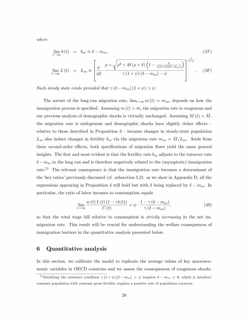
Such steady state exists provided that 1 (. "mss) (1 + ) > .
The nature of the long-run migration rate, limt!1m (t) = mss, depends on how the
immigration process is speciÖed. Assuming m (t) = ,m, the migration rate is exogenous and
our previous analysis of demographic shocks is virtually unchanged. Assuming M (t) = ,M ,
the migration rate is endogenous and demographic shocks have slightly richer e§ects ñ
relative to those described in Proposition 3 ñ because changes in steady-state population
Lss also induce changes in fertility bss via the migration rate mss = ,M=Lss. Aside from
these second-order e§ects, both speciÖcations of migration áows yield the same general
insights. The Örst and most evident is that the fertility rate bss adjusts to the turnover rate
."mss in the long run and is therefore negatively related to the (asymptotic) immigration
rate.21 The relevant consequence is that the immigration rate becomes a determinant of
the ëkey ratiosí previously discussed (cf. subsection 5.2): as we show in Appendix D, all the
expressions appearing in Proposition 4 will hold but with . being replaced by . "mss. In
particular, the ratio of labor incomes to consumption equals
limt!1
w (t)L (t) (1" 1b (t))C (t)
= $1" 1 (. "mss)
1 (. "mss); (49)
so that the total wage bill relative to consumption is strictly increasing in the net im-
migration rate. This result will be crucial for understanding the welfare consequences of
immigration barriers in the quantitative analysis presented below.
6 Quantitative analysis
In this section, we calibrate the model to replicate the average values of key macroeco-
nomic variables in OECD countries and we assess the consequences of exogenous shocks.
21Satisfying the existence condition 0 (1 + ) (' "mss) > requires ' " mss > 0, which is intuitive:
constant population with constant gross fertility requires a positive rate of population turnover.
28
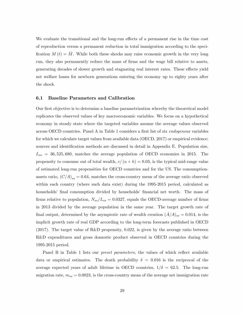
We evaluate the transitional and the long-run e§ects of a permanent rise in the time cost
of reproduction versus a permanent reduction in total immigration according to the speci-
Öcation M (t) = ,M . While both these shocks may raise economic growth in the very long
run, they also permanently reduce the mass of Örms and the wage bill relative to assets,
generating decades of slower growth and stagnating real interest rates. These e§ects yield
net welfare losses for newborn generations entering the economy up to eighty years after
the shock.
6.1 Baseline Parameters and Calibration
Our Örst objective is to determine a baseline parametrization whereby the theoretical model
replicates the observed values of key macroeconomic variables. We focus on a hypothetical
economy in steady state where the targeted variables assume the average values observed
across OECD countries. Panel A in Table 1 considers a Örst list of six endogenous variables
for which we calculate target values from available data (OECD, 2017) or empirical evidence:
sources and identiÖcation methods are discussed in detail in Appendix E. Population size,
Lss = 36; 525; 680, matches the average population of OECD economies in 2015. The
propensity to consume out of total wealth, c= (a+ h) = 0:03, is the typical mid-range value
of estimated long-run propensities for OECD countries and for the US. The consumption-
assets ratio, (C=A)ss = 0:64, matches the cross-country mean of the average ratio observed
within each country (where such data exist) during the 1995-2015 period, calculated as
householdsí Önal consumption divided by householdsí Önancial net worth. The mass of
Örms relative to population, Nss=Lss = 0:0327, equals the OECD-average number of Örms
in 2013 divided by the average population in the same year. The target growth rate of
Önal output, determined by the asymptotic rate of wealth creation ( _A=A)ss = 0:014, is the
implicit growth rate of real GDP according to the long-term forecasts published in OECD
(2017). The target value of R&D propensity, 0:022, is given by the average ratio between
R&D expenditures and gross domestic product observed in OECD countries during the
1995-2015 period.
Panel B in Table 1 lists our preset parameters, the values of which reáect available
data or empirical estimates. The death probability . = 0:016 is the reciprocal of the
average expected years of adult lifetime in OECD countries, 1=. = 62:5. The long-run
migration rate, mss = 0:0023, is the cross-country mean of the average net immigration rate
29
observed within each economy during the 1973-2012 period. In the simulations, we match
this target by setting the mass of immigrants ,M = 84; 009. The value of the elasticity of
substitution across intermediates, ? = 4:3, implies a mark-up for monopolistic Örms equal
to 1:3, in the middle of the range 1:2-1:4 suggested by international evidence.22 The rates
of time preference and product obsolescence, - and H, are set so as to obtain plausible
values of interest rates, private returns to householdsí assets, and proÖt discount rates for
Örms. The combination - = 1:5% and H = 1% generates the equilibrium interest rate
rss = 2:98% and, hence, a fair-annuity rate (r + .) on householdsí assets of 4:6%, and a
proÖt-discount rate (r+H) for Örms of 4% in the steady state. The value of @"1 represents
the elasticity of productivity to the mass of intermediate goods, a parameter for which Broda
et al. (2006) provide structural estimates ranging from 0:05 to 0:20, where the lower bound
applies to advanced economies and the upper bound to developing countries.23 We adopt
a conservative approach by setting initially the baseline value on the low end, @" 1 = 0:05,
and then perform a sensitivity analysis with alternative values in the range 0:025-0:10. For
parameter {, we set a baseline value of zero and then check the robustness of our results
under alternative values.
Given the preset parameters, we calibrate the remaining six parameters listed in Panel
C of Table 1 so as to match the six target values of the endogenous variables listed in
Panel A. First, we consider the demographic block of the model: since the values . and
mss already determine steady state fertility bss, we identify (1; ; K) by imposing the target
values of Lss, (C=A)ss and c= (a+ h) in the respective equations (360), (39) and (10). Con-
sidering the supply-side, we identify ('; !; D) by imposing the target values of Nss=Lss and
( _A=A)ss in equations (44) and (46), respectively, and by setting the target value of the R&D
propensity, 2:2%, equal to the steady-state ratio between total wages paid to non-production
22The range 1:2-1:4 captures most estimates of economy-wide mark-ups for the US and UK economies ñ
see Britton et al. (2000) and the further references cited in Appendix E. The empirical literature shows
that sectoral mark-ups may obey wider ranges, with mean values typically higher in services and lower in
manufacturing.23There is growing empirical literature on trade estimating the ëgains from variety expansioní from highly
disaggregated data on imported goods. Such estimates are highly model-speciÖc (see Feenstra, 2010) and
most econometric models identify such gains with a ëlove-for-varietyí parameter that appears in Dixit-Stiglitz
preferences. Our theoretical model, instead, identiÖes the gains from variety with a technology parameter
for which the closest empirical counterpart is the ëelasticity of productivity to varietyí calculated by Broda
et al. (2006).
30
workers, w (`N + `Z), and aggregate income calculated from the budget constraint (7). This
procedure yields the calibrated values of the parameters reported in Table 1, Panel C.
6.2 Steady State Results
The Örst row of panel D in Table 1 reports the steady-state values of the main variables of
interest under the baseline parametrization. Besides the targeted values already discussed,
we obtain the gross fertility rate bss = 1:37% implied by the demographic law, and a ratio of
total labor incomes to assets (w~L=A)ss = 0:62 that is empirically plausible. The same panel
considers six alternative parametrizations showing how the steady state changes in response
to ceteris paribus variations in demographic parameters. The numerical results for higher
mortality and stronger impatience conÖrm and extend our analytical Öndings (subsect. 5.3)
on the opposite e§ects of . and -: besides population and labor incomes relative to assets,
also the mass of Örms and the long-run growth rates move in opposite directions in response
to the two shocks.
The third and fourth scenarios emphasize, instead, the similar consequences of reduc-
tions in ,M and increases in 1. Reduced immigration and increased reproduction costs
produce a qualitatively di§erent response of the fertility rate. The reduction in ,M increases
bss because a permanent fall in net ináows is ultimately compensated by increased domestic
births in the steady state. The increase in 1, instead, reduces transitional fertility rates
via higher private costs of reproduction leaving the long-run rate bss unchanged. Despite
the asymmetric fertility response, the two shocks bear qualitatively identical consequences
on the other endogenous variables. Reduced immigration and increased reproduction costs
reduce the long-run population level and drive down labor incomes relative to assets; the
long-run mass of Örms shrinks, and the reallocation of workers to vertical R&D boosts in-
terest rates in the long run. Although both migration and child-cost shocks enhance wealth
creation in the long run, the welfare consequences of such shocks are neither clear-cut nor
symmetric across generations: we investigate this point in the next subsection by studying
both the transitional and the long-run e§ects of large permanent shocks.
6.3 Demographic Shocks, Transition and Welfare
The calibrated model allows us to evaluate the transitional e§ects of exogenous shocks and
their impact on intergenerational welfare. Di§erently from Table 1, this subsection considers
31

large unexpected permanent shocks. We set year 2015 as our reference time zero and assume
that the shocks hit the ëaverage OECD economyí from year 2020 onwards. We focus on
the two scenarios of ëreduced immigrationí and ëincreased reproduction costí bearing similar
quantitative e§ects on steady-state population. The Örst scenario assumes amigration shock
whereby the net ináows ,M fall permanently by 25% of the baseline value, from 84; 009 to
63; 006, which may be interpreted as an ëimmigration barrierí set by a policymaker. The
second scenario assumes a child-cost shock whereby 1 permanently increases by 6% of its
baseline value.
Panel A in Table 2 provides a summary comparison of the migration and child-cost
shocks in terms of initial, short-to-medium-run and steady-state e§ects on selected variables.
Figure 2 presents a detailed analysis of the transitional paths generated by the two shocks
over a century-long horizon. As already noted, besides the di§erent response of fertility
rates, the two shocks produce qualitatively identical dynamics for all the variables of interest.
The important new insight delivered by Table 2 and Figure 2 is that the impact of both
shocks on growth-related variables in the short-to-medium run is reversed with respect to
the steady state outcomes. Although reduced migration and increased reproduction costs
raise wealth creation and interest rates in the very long run, the transition features several
decades of slower growth and reduced rates of return. The reason is that the decline in
population creates net exit of Örms from the market during the whole transition, _N=N < 0,
and the decline in the rate of horizontal innovations reduces wealth creation, _A=A, in the
short-to-medium run. By the same mechanism, during the Örst part of the transition,
interest rates decline and labor is reallocated from entry to production activities. The
scope of these transitional e§ects is substantial because the convergence to the new steady
state is slow. The bottom panel in Figure 2 shows that the negative demographic shocks
substantially reduce aggregate consumption in the medium run: the smaller drop and the
subsequent recovery that we observe in consumption per capita during this phase is actually
due to the population decline rather than to faster output growth.
The existence of prolonged ëreversed growth e§ectsí during the transition bears conse-
quences for intergenerational welfare: the same shock may a§ect di§erent cohorts in oppo-
site ways. The Örst key question relates to the intensity and persistence of such reversed
growth e§ects. In this respect, a crucial parameter is @, which determines the relative
contribution of the Örmsí net entry rate, _N=N , to the economyís rate of wealth creation,
32
_A=A. The transition paths in Figure 2 assume the benchmark value @ = 1:05 and show
that the reversed e§ect on wealth creation lasts 70 years: after the shock occurring in 2020,
the growth rate of assets is below the baseline level until 2090. Assuming higher (lower)
values of @ would further delay (anticipate) the switching date, i.e., the instant at which
_A=A crosses the pre-shock level from below. We investigate this point by setting alternative
values for @ in a sensitivity analysis that addresses the second key question, namely, the
welfare consequences of reversed growth e§ects.
Generations that happen to be alive when the shocks occur may experience net welfare
losses despite the fact that such shocks are growth-enhancing in the long run. New cohorts
entering the economy immediately after the shocks are particularly exposed because they
heavily rely on labor incomes (newborn agents have zero Önancial wealth) and experience
a productivity slowdown that reduces real wages for decades (with respect to the pre-shock
baseline path). We tackle this aspect by calculating the value of a cohort-speciÖc utility
index,
EPWj %Z j+(1=$)
j[ln cj (t) + ln bj (t)] $ e%#(t%j)dt; (50)
which represents the ex-post welfare level enjoyed by a typical member of cohort j whose
actual lifetime exactly coincides with life expectancy 1=.. Table 2, panel B, reports the
values of EPWj for ten di§erent cohorts born in the years j = 2025; 2035; :::; 2115, and
compares their welfare levels in the three cases of interest: the ëno shockí scenario in which
the economy remains in the baseline steady state forever, the migration shock, and the
child-cost shock. We repeat this exercise under the alternative values @ = (1:025; 1:05; 1:10),
where 1:05 is our benchmark, assuming the same initial stock of knowledge in all scenarios.24
The general, robust conclusion delivered by Table 2 is that both shocks are welfare-reducing
for a large set of newborn generations. All the cohorts born within a century after the child-
cost shock su§er net welfare losses in the cases @ = (1:05; 1:10). Assuming @ = 1:025, we
observe net welfare gains for the cohorts born after 2100. The bottom-line is that although
increased reproduction costs and reduced immigration may raise economic growth in the
very long run, the transition to the new steady state features many decades of slower growth
and lower lifetime utility for a long sequence of newborn generations.
24The numbers appearing in Table 2, panel B, are obtained by setting initial knowledge (at the time of the
shock) equal to the value Z (2020) = 478 # 10$6 in all parametrizations; this value is chosen fro convenience
as it yields a normalized level of consumption per capita c (2015) = 1 under ; = 1:025.
33
7 Conclusion
The interaction between wealth dilution caused by disconnected generations and wealth
creation driven by vertical and horizontal innovations delivers a theory of the population
level that fully abstracts from Malthusian mechanisms. The nature of the economyís steady
state, which features a constant endogenous population level and sustained endogenous
output growth, suggests a novel, demography-based view of the long run equilibrium: de-
mographic change originating in exogenous shocks that a§ect reproduction costs, life ex-
pectancy and migration, have a Örst-order impact on the functional distribution of income,
productivity growth and intergenerational welfare. Our results challenge several predictions
of traditional growth models and open the door to a wide set of quantitative applications to
assess the macroeconomic impact of demographic phenomena and related public policies ñ
e.g., population ageing and pension systems, child-cost subsidies and immigration policies
ñ in a framework where output growth and the population level are closely interconnected
even in the long run.
References
Aghion, P., Howitt, P. (1992). A Model of Growth Through Creative Destruction. Econo-
metrica 60 (2): 323-351.
Barro, R., Becker, G. (1989). Fertility Choice in a Model of Economic Growth. Econo-
metrica 57 (2): 481-501.
Blanchard, O. (1985). Debt, DeÖcits, and Finite Horizons. Journal of Political Economy
93: 223-247.
Bloom, D., Canning, D., Sevilla, J. (2003). The Demographic Dividend. RAND Corpora-
tion.
Brander, J., Taylor, M.S. (1998). The Simple Economics of Easter Island: A Ricardo-
Malthus Model of Renewable Resource Use. American Economic Review 88 (1):
119-38.
Britton, E., Larsen, J., Small, I. (2000). Imperfect competition and the dynamics of
markups. Bank of England working papers 110, Bank of England.
34

Broda, C., GreenÖeld, J., Weinstein, D. (2006). From Groundnuts to Globalization: A
Structural Estimate of Trade and Growth. NBER Working Papers 12512, National
Bureau of Economic Research.
Buiter, W. (1988). Death, Birth, Productivity Growth and Debt Neutrality. Economic
Journal 98: 279-293.
Chu, A., Cozzi, G., Liao, C.-H. (2013). Endogenous fertility and human capital in a
Schumpeterian growth model. Journal of Population Economics 26: 181-202.
Dinopoulos, E., Thompson, P. (1998). Schumpeterian Growth without Scale E§ects. Jour-
nal of Economic Growth 3 (4): 313-335.
Eckstein, Z., Stern, S., Wolpin, K. (1988). Fertility choice, land, and the Malthusian
hypothesis. International Economic Review 29: 353-361.
Ehrlich, I., Lui, F. (1997). The problem of population and growth: A review of the litera-
ture from Malthus to contemporary models of endogenous population and endogenous
growth. Journal of Economic Dynamics and Control 21 (1): 205-242.
Faruqee, H. (2002). Population Ageing and its Macroeconomic Implications: A Framework
for Analysis. IMF Working Paper 02/16.
Feenstra, R. (2010). Measuring the Gains from Trade under Monopolistic Competition.
Canadian Journal of Economics 43 (1): 1-28.
Galor, O., Weil, D. (2000). Population, Technology, and Growth: From Malthusian Stag-
nation to the Demographic Transition and Beyond. American Economic Review 90
(4): 806-828.
Howitt, P. (1999). Steady Endogenous Growth with Population and R&D Inputs Growing.
Journal of Political Economy 107 (4): 715-730.
Lucas, R. (2002). Lectures on Economic Growth. Cambridge, MA: Harvard University
Press.
OECD (2017). OECD Statistics, www.stats.oecd.org (accessed July 2017). Organisation
for Economic Co-operation and Development.
35
Peretto, P. (1998). Technological Change and Population Growth. Journal of Economic
Growth 3: 283-311.
Peretto, P., Connolly, M. (2007). The manhattan metaphor. Journal of Economic Growth
12 (4): 329-350.
Peretto, P., Smulders, S. (2002). Technological distance growth and scale e§ects. Economic
Journal 112: 603-624.
Peretto, P., Valente, S. (2015). Growth on a Önite planet: resources, technology and
population in the long run. Journal of Economic Growth 20: 305-331.
Romer, P. (1986). Increasing Returns and Long-run Growth. Journal of Political Economy
94 (5): 1002-1037.
Romer, P. (1990). Endogenous Technological Change. Journal of Political Economy 98
(5): 71-102.
Solow, R. (1956). A Contribution to the Theory of Economic Growth. Quarterly Journal
of Economics 70 (1): 65-94.
Strulik, H., Weisdorf, J. (2008). Population, Food, and Knowledge: A Simple UniÖed
Growth Theory. Journal of Economic Growth 13 (3): 195-216.
Weil, P. (1989). Overlapping families of inÖnitely-lived agents. Journal of Public Eco-
nomics 38 (2): 183-198.
Wrigley, E.A. (1988). Continuity, Chance and Change. Cambridge: Cambridge University
Press.
Yaari, M. (1965). Uncertain Lifetime, Life Insurance, and the Theory of the Consumer.
Review of Economic Studies 32: 137-150.
36
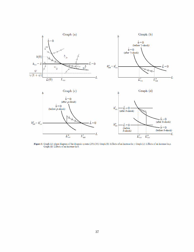
37
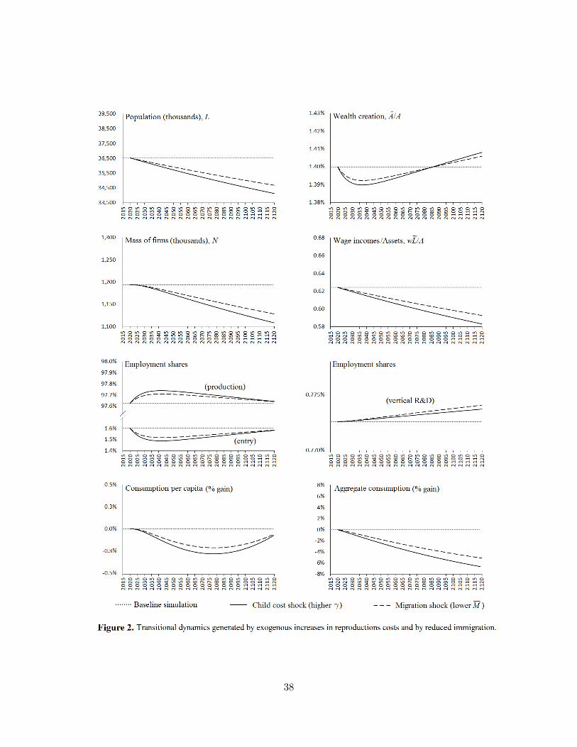
38
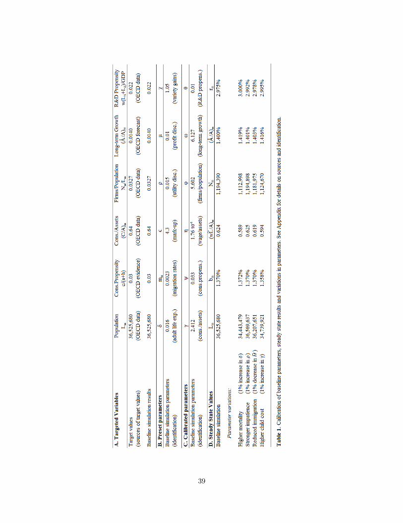
39
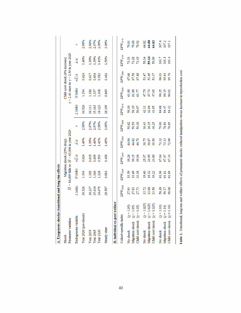
40
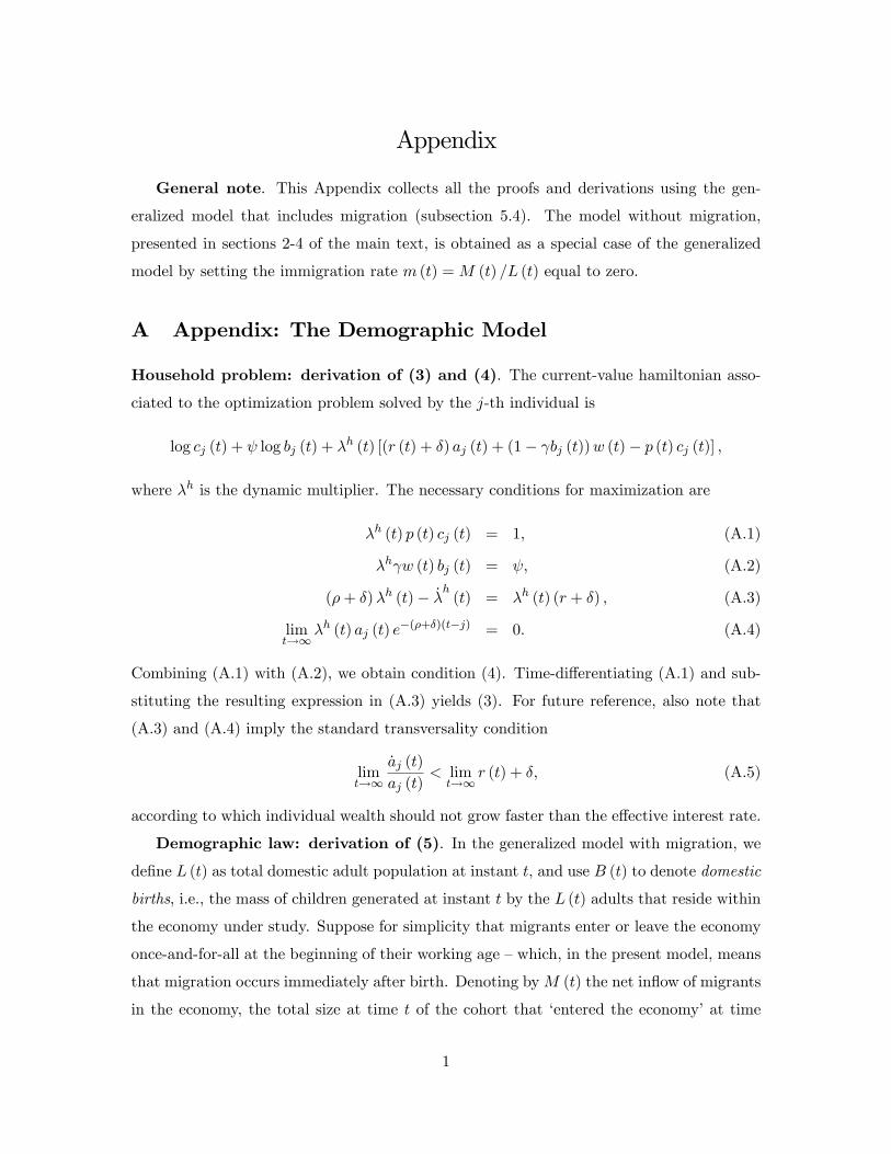
Appendix
General note. This Appendix collects all the proofs and derivations using the gen-
eralized model that includes migration (subsection 5.4). The model without migration,
presented in sections 2-4 of the main text, is obtained as a special case of the generalized
model by setting the immigration rate m (t) =M (t) =L (t) equal to zero.
A Appendix: The Demographic Model
Household problem: derivation of (3) and (4). The current-value hamiltonian asso-
ciated to the optimization problem solved by the j-th individual is
log cj (t) + log bj (t) + Th (t) [(r (t) + .) aj (t) + (1" 1bj (t))w (t)" p (t) cj (t)] ;
where Th is the dynamic multiplier. The necessary conditions for maximization are
Th (t) p (t) cj (t) = 1; (A.1)
Th1w (t) bj (t) = ; (A.2)
(-+ .)Th (t)" _Th(t) = Th (t) (r + .) ; (A.3)
limt!1
Th (t) aj (t) e%(#+$)(t%j) = 0: (A.4)
Combining (A.1) with (A.2), we obtain condition (4). Time-di§erentiating (A.1) and sub-
stituting the resulting expression in (A.3) yields (3). For future reference, also note that
(A.3) and (A.4) imply the standard transversality condition
limt!1
_aj (t)
aj (t)< lim
t!1r (t) + .; (A.5)
according to which individual wealth should not grow faster than the e§ective interest rate.
Demographic law: derivation of (5). In the generalized model with migration, we
deÖne L (t) as total domestic adult population at instant t, and use B (t) to denote domestic
births, i.e., the mass of children generated at instant t by the L (t) adults that reside within
the economy under study. Suppose for simplicity that migrants enter or leave the economy
once-and-for-all at the beginning of their working age ñ which, in the present model, means
that migration occurs immediately after birth. Denoting byM (t) the net ináow of migrants
in the economy, the total size at time t of the cohort that ëentered the economyí at time
1
j is denoted by kj (t). By construction, the size of cohort j at instant j equals the sum of
domestic o§spring and immigrants,
kj (j) = B (j) +M (j) : (A.6)
Assuming that foreign immigrants exhibit the same death probability . and the same pref-
erence for fertility as domestic residents, the size of cohort j at time t is then given by
kj (t) = kj (j) $ e%$(t%j) = [B (j) +M (j)] $ e%$(t%j): (A.7)
Given the deÖnitions of total adult population and domestic births
L (t) %Z t
%1kj (t) dj and B (t) %
Z t
%1kj (t) bj (t) dj; (A.8)
Using (A.6) to substitute kj (t) in the deÖnition of L (t), and di§erentiating the resulting
expression with respect to t, we obtain the generalized demographic law
_L (t) = B (t) +M (t)" .L (t) : (A.9)
Setting net migration to zero, M (t) = 0, we have expression (5), i.e., the demographic law
used in section 2. In the generalized model with migration, we deÖne the net immigration
rate m (t) %M (t) =L (t) and rewrite the demographic law (A.9) as
_L (t)
L (t)= b (t) +m (t)" .: (A.10)
Aggregate wealth constraint: derivation of (7). Total assets and aggregate con-
sumption are deÖned as
A (t) %Z t
%1kj (t) aj (t) dj and C (t) %
Z t
%1kj (t) cj (t) dj: (A.11)
From (A.11), the time-derivative of A (t) equals
_A (t) =ddt
Z t
%1kj (t) aj (t) dj = kt (t) at (t) +
Z t
%1
hkj (t) _aj (t) + _kj (t) aj (t)
idj;
where we can substitute at (t) = 0 (i.e., people entering the economy have zero assets and
receive no bequests), as well as the transition law of cohort size _k (j; t) = ".k (j; t) from
(A.7), to obtain
_A (t) =
Z t
%1kj (t) _aj (t) dj " .A (t) : (A.12)
2

Using the budget constraint (2) to substitute _aj (t), and aggregating, expression (A.12)
yields
_A (t) =
Z t
%1k (j; t) [(r (t) + .) $ a (j; t) + (1" 1b (j; t)) $ w (t)" p (t) c (j; t)] dj " .A (t) =
= (r (t) + .) $A (t) + w (t)L (t)" w (t) 1B (t)" p (t)C (t)" .A (t) ; (A.13)
which, dividing both sides by A (t), reduces to expression (7) in the main text.
Individual expenditure: derivation of (9). Integrating the individual budget con-
straint (2) forward in time, we obtain
aj (t) =
Z 1
t[p (s) cj (s)" (1" 1bj (s))w (s)] $ e%
R st (r(v)+$)dvds:
Using (4) to substitute 1b (j; s)w (s), and rearranging terms, the above expression yields
aj (t) +
Z 1
tw (s) $ e%
R st (r(v)+$)dvds = (1 + )
Z 1
tp (s) cj (s) $ e%
R st (r(v)+$)dvds: (A.14)
From the Keynes-Ramsey rule (3), we substitute p (s) cj (s) = p (t) cj (t) $ eR st (r(v)%#)dv in
(A.14) and solve the residual integral, obtaining
aj (t) +
Z 1
tw (s) $ e%
R st (r(v)+$)dvds =
1 +
-+ .$ p (t) cj (t) ; (A.15)
which is expression (9) in the text.
Per capita expenditure: derivation of (10). Multiplying both sides of (A.15) by
the size of cohort j, and integrating across cohorts, we obtain
1
-+ .$ (1 + ) p (t) $
Z t
%1kj (t) $ cj (t) dj
| {z }C(t)
=
Z t
%1kj (t) $ aj (t) dj
| {z }A(t)
+
Z t
%1kj (t)h (t) dj; (A.16)
where C (t) is aggregate consumption as deÖned in (A.11). Since h (t) is independent of j,
we can rewrite (A.16) as
1
-+ .(1 + ) p (t)C (t) = A (t) + h (t)
Z t
%1kj (t) dj
| {z }L(t)
;
which, dividing both sides by L (t), reduces to expression (7) in the main text.
Per capita consumption growth: derivation of (11). Substituting (4) to substitute
B (t) in (A.13), we have
_A (t) = r (t)A (t) + w (t)L (t)" (1 + ) p (t)C (t) : (A.17)
3
Equation (A.17) implies
A (t)
L (t)$
_A (t)
A (t)"_L (t)
L (t)
!=r (t)A (t)
L (t)+ w (t)" (1 + )
p (t)C (t)
L (t)"A (t)
L (t)$_L (t)
L (t): (A.18)
From the deÖnition of human wealth h (t) =R1t w (s) $ e%
R st (r(v)+$)dvds, we have the time
derivative
_h (t) = (r (t) + .) $ h (t)" w (t) : (A.19)
Given these results, time-di§erentiate (10) to obtain
dp (t) c (t)dt
=-+ .
1 +
"A (t)
L (t)
_A (t)
A (t)"_L (t)
L (t)
!+ _h (t)
#;
where we can substitute (A.18) and (A.19), along with _L (t) = B (t) +M (t)" .L (t) from
(A.9), to get
dp (t) c (t)dt
=-+ .
1 + $'(r (t) + .)
)A (t)
L (t)+ h (t)
*" (1 + )
p (t)C (t)
L (t)"A (t)
L (t)
)B (t)
L (t)+m (t)
*(:
(A.20)
Substituting B (t) = 4 $
p(t)C(t)w(t) from (6) in (A.20), and dividing both sides by pcc % pC=L
using (10), we have
dp (t) c (t)dt
$1
p (t) c (t)= r (t)" -"
'-+ .
1 +
)
1
1
w (t)+
m (t)
p (t) c (t)
*(A (t)
L (t): (A.21)
Re-arranging the left hand side of (A.21) yields
_c (t)
c (t)+_p (t)
p (t)= r (t)" -"
-+ .
1 +
)
1
1
w (t)+
m (t)
p (t) c (t)
*a (t) ; (A.22)
which holds in the generalized model with migration. Setting m (t) = 0 in (A.22) gives
expression (11) in the main text.
Fertility dynamics: derivation of (14). Time-di§erentiation of (13) gives
_b (t)
b (t)=_c (t)
c (t)+_p (t)
p (t)"_w (t)
w (t); (A.23)
where we can substitute (A.22) to obtain
_b (t)
b (t)= r (t)" -"
-+ .
1 +
)
1
1
w (t)+
m (t)
p (t) c (t)
*a (t)"
_w (t)
w (t): (A.24)
From the dynamic wealth constraint (7), the interest rate may be expressed as
r (t) =_A (t)
A (t)"w (t)L (t)
A (t)+w (t) 1B (t)
A (t)+p (t)C (t)
A (t);
4

or, equivalently,
r (t) =_a (t)
a (t)+_L (t)
L (t)"w (t)
a (t)+ 1
w (t) b (t)
a (t)+p (t) c (t)
a (t): (A.25)
Plugging (A.25) into (A.24) to eliminate r (t), we have
_b
b=_a
a+_L
L"w
a+ 1
wb
a+pc
a" -"
-+ .
1 +
)
1
1
w+m
pc
*a"
_w
w;
where we can use (A.10) to substitute _L=L, and substitute pc = b1w= from (13), obtaining
_b
b= b
)1 + 1
1 +
w
a
*+m" -" . "
-+ .
1 +
)
1
1
w+m
pc
*a"
w
a+_a
a"_w
w; (A.26)
which holds in the generalized model with migration. Setting m = 0 in (A.26) gives expres-
sion (14) in the main text.
Alternative Supply-Side Structures (subsection 2.4): (ii) Neoclassical models
with physical capital. In neoclassical models, aggregate Önancial wealth coincides with
the economyís capital stock K employed in production with labor under constant returns to
scale. Assume for simplicity the Cobb-Douglas production function Y = KB [(1" 1b)L]1%B
where (1" 1b)L is net labor supply. ProÖt maximization in the production sector im-
ply that a=w = (1" 1b) = (1" W) in each instant, where a = K=L is assets per capita.
Substituting this result into the core fertility equation (14), we have
_b (t)
b (t)= b (t)
)1" 1b (t) + 1
(1 + ) (1" W)
*"(-+ .) (1" 1b (t))"(1" W)"
(-+ .)
1 (1 + ) (1" W)$(1" 1b (t))2
which is an autonomous equation in the fertility rate: denoting the right hand side by ~f (b),
the steady-state locus _b = 0 is represented by ~f (b) = 0 with
@ ~f (b)
@b> 0; lim
b!+1~f (b) = +1;
limb!0
~f (b) = " (-+ . + 1" W)" (-+ .)
1 (1 + ) (1" W)< 0;
implying a unique unstable steady state bss that satisÖes ~f (bss) = 0 and that is generally
di§erent from .. We thus have the result that, combining the demographic structure of
section 2 with the supply side of neoclassical models, the fertility rate jumps at the sta-
tionary value bss and is constant thereafter: the economy features endogenous constant
population growth, which ìpullsî constant aggregate capital growth in the long run, in line
with the traditional notion of balanced growth. This result implies that combining our
5
demographic structure with a neoclassical production structure does not produce a theory
of the population level (the very special case in which bss coincides with . may only happen
by chance).
Alternative Supply-Side Structures (subsection 2.4): (iii) Constant returns
to physical capital. Consider the following model with learning-by-doing as a modiÖcation
of the neoclassical case discussed above. At the aggregate level, output is given by Y =
KB [T $ (1" 1b)L]1%B where T is labor productivity determined by an externality to be
speciÖed later, and wealth per capita is a = K=L. In this case, proÖt maximization with
respect to employed labor units (1" 1b)L yields w = (1" W)KBT 1%B (1" 1b)%B L%B and,
hence, the ratio
a=w =(1" 1b)B
(1" W)L1%B$K1%B
T 1%Bwith T =
8<
:T(1) % K= [L (1" 1b)]
T(2) % K
where T(1) and T(2) are two alternative speciÖcations of the learning-by-doing externality
that capture the polar cases considered in the growth literature. SpeciÖcation T = T(2)
follows Romerís (1986) model in assuming that labor productivity grows with the aggregate
capital stock, and implies the strong scale e§ect, namely, the prediction that population size
increases permanently the economyís growth rate. SpeciÖcation T = T(1) assumes, instead,
that the externality is determined by the capital to labor ratio and is the easiest way to
eliminate the strong scale e§ect from this class of models with constant returns to capital.25
Considering T = T(1) = K= [L (1" 1b)], the wealth-wage ratio reduces to
a=w(1) =1" 1b1" W
;
which is exactly the same result holding in the neoclassical models discussed above, implying
that the fertility rate jumps at the stationary value bss and is constant thereafter. Therefore,
the endogenous growth model with constant returns to capital under speciÖcation T(1) does
not produce a theory of the population level (the very special case in which bss coincides
with . may only happen by chance). Next, consider T = T(2) = K as in Romer (1986). In
this case, we have
a=w(2) =(1" 1b)B
(1" W)L1%B;
_a
a"_w
w= "W
1 _b
1" 1b" (1" W)
_L
L;
25A more general speciÖcation to obtain a scale-free model is T ! K= [L (1" 0b)]*/, which would not
change our conclusions: we concentrate on the case /> = 1 to preserve clarity.
6
which may be substituted in the core fertility equation (14) to obtain
_b
b=
1
1 + Bb1%4b
'Wb+
b1 (1 + )"
$(1" W)L1%B
(1" 1b)B" -" W. "
(-+ .)
1 (1 + )$(1" 1b)B
(1" W)L1%B
(:
(A.27)
From (A.27), a steady state with constant fertility (_b = 0) and constant population (b = .)
requires satisfying
. +1" W
(1" 1.)B
'1. (1 + )"
($ L1%Bss = -+ . +
(-+ .)
1 (1 + )$(1" 1.)B
(1" W)$1
L1%Bss(A.28)
which shows that a positive steady-state population level Lss > 0 exists provided that
1. (1 + ) > . However, in such a steady state with constant population, the economyís
growth rate26_Y
Y=
_K
K=Y
K"C
K= [(1" 1bss)Lss]1%B "
1
bssa=w(2)
(A.29)
can be rewritten as_Y
Y=1" 1. " 1%B
1.
(1" 1.)B$ L1%Bss : (A.30)
Expression (A.27) delivers two main results. First, by combining the existence condition in
(A.28) with the numerator in the right hand side of (A.30), we see that the existence of a
steady state with constant population and constant output growth requires that parameters
satisfy
1. (1 + " W) < < 1. (1 + ) ; (A.31)
where the Örst inequality is the requirement for positive output growth and the second
inequality is necessary for Lss > 0 to exist. Since the plausible range of values for W
typically lies between 0.2 and 0.6, the set of parametrizations satisfying (A.31) is extremely
narrow. The Örst conclusion is thus that if a steady-state with constant population under
Romerís (1986) speciÖcation T = T , it is very unlikely to generate strictly positive output
growth. The second conclusion is that the growth rate (A.30) is a§ected by the strong
scale e§ect: in this model, any positive (negative) shock on the population level increases
(decreases) permanently the economyís growth rate.
26The last term in (A.29) are given by CK= +
bwa, which follows from combining result (13) with a = K=L.
7
B Appendix: The Production Side
ProÖt maximization in the Önal sector. The proÖts of the Önal sector read
p (t)C (t)"Z N(t)
0pxi (t)xi (t) di = N (t))%
$$$1 $
Z N(t)
0xi (t)
$$1$ di
! $$$1
"Z N(t)
0pxi (t)xi (t) di;
and the Örst order conditions with respect to each quantity xi read
p (t)N (t))%$$$1 $
Z N(t)
0xi (t)
$$1$ di
! $$$1%1
$ xi (t)%1$ = pxi (t) : (B.1)
Using technology (15), expression (B.1) may be rewritten as
pxi (t) =p (t)C (t)
R N(t)0 xi (t)
$$1$ di
$ xi (t)%1$ = ;c (t)xi (t)
% 1$ (B.2)
where we have deÖned the term ;c % pC=R N0 xi
$$1$ di.
Intermediate Producers: the incumbentís problem. The instantaneous proÖts
of the typical monopolist read
Zxi (t) % pxi (t)xi (t)" w (t) `xi (t)" w (t) `zi (t) : (B.3)
From the production function (17), labor employed in intermediate production by each
incumbent Örm equals
`xi (t) = xi (t) zi (t)%- + ': (B.4)
Using (B.4) and the demand schedule (B.2), we can rewrite the monopolist instantaneous
proÖts (B.3) as
Zxi (t) = ;c (t)xi (t)$$1$ " w (t) [xi (t) zi (t)%- + ']" w (t) `zi (t) ; (B.5)
where the term ;c % pC=R N0 xi
$$1$ di is taken as given by the i-th monopolist. Given the
knowledge accumulation law (18), the incumbent solves the problem
maxfxi(t);`zi(t)g
Vi (t) =
Z 1
tZxi (v) e
%R vt (r(s)+0)dsdv subject to _zi (t) = !Z (t) $ `zi (t)
where public knowledge Z (t) is also taken as given. The current-value hamiltonian at
instant v associated with this problem is
;c (v)xi (v)$$1$ " w (v) [xi (v) zi (v)%- + ']" w (v) `zi (v) + Ti (v)!Z (v) `zi (v) ;
8
where Ti is the dynamic multiplier, xi and `zi are control variables, and zi is the state
variable. The necessary conditions for maximization read
?" 1?;c (v)xi (v)
% 1$ = w (v) zi (v)
%- ; (B.6)
Ti (v)!Z (v) = w (v) ; (B.7)_Ti (v)
Ti (v)= r (v) + H" D
w (v)
Ti (v)xi (v) zi (v)
%-%1 : (B.8)
In the left hand side of (B.6), we can substitute ;cxi%1$ = pxi from (B.2) to obtain the
mark-up rule for the intermediate goodís price at each instant t,
pxi (t) =?
?" 1w (t) zi (t)
%- : (B.9)
Multiplying both sides of (B.9) by xi and substituting the technology (17), we obtain the
proÖt-maximizing value of intermediate production
pxi (t)xi (t) =?
?" 1$ w (t) (`xi (t)" ') : (B.10)
Time-di§erentating (B.7) and substituting the resulting expression in (B.8) to eliminate
Ti=Ti, we have
_w (t)
w (t)"_Z (t)
Z (t)= r (v)+H" D!Z (t)xi (t) zi (t)%-%1 = r (t)+H" D!Z (t)
`xi (t)" 'zi (t)
; (B.11)
where the central term makes use of (B.7) to eliminate Ti, and the last term follows from
(B.4). Using (B.10) to eliminate `xi " ' from (B.11), and rearranging terms, yields
r (t) + H = D?" 1?
pxi (t)xi (t)
zi (t)!Z (t)
w (t)+_w (t)
w (t)"_Z (t)
Z (t)(B.12)
which is the Örmís rate of return to vertical innovation shown as (21) in the main text.
Symmetric equilibrium. Our speciÖcation of public knowledge (19) implies that
each Örm faces equal initial conditions besides exploiting the same technology. Therefore,
intermediate sector operates in a symmetric equilibrium where each Örm i 2 [0; N (t)]
exhibits
zi (t) = Z (t) ; (B.13)
xi (t) = Z (t)- $ (`xi (t)" ') ; (B.14)
pxi (t) =?
?" 1w (t)Z (t)%- ; (B.15)
9
at each point in time. From (15), symmetry implies that aggregate Önal output equals
C (t) = N (t))%$$$1 $
Z N(t)
0xi (t)
$$1$ di
! $$$1
= N (t)) xi (t) : (B.16)
From the demand schedule (16), we have
xi (t) =p (t)C (t)
N (t) pxi (t): (B.17)
Combining (B.16) with (B.17), the price of intermediates is
pxi (t) = p (t)N (t))%1 : (B.18)
Moreover, from (B.14) and (B.17), we have the aggregate value of Önal output as
p (t)C (t) = N (t) pxi (t)Z (t)- $ (`xi (t)" ') ;
where we can substitute pxi using (B.14), obtaining
C (t) = N (t))%1 $ Z (t)- $ [N (t) `xi (t)"N (t)'] : (B.19)
Labor market clearing: equation (24). Symmetry in the intermediate sector implies
that aggregate employment in intermediate production and in vertical R&D equals
Z N(t)
0(`xi (t) + `zi (t)) di = N (t) `xi (t) +N (t) `zi (t) :
Including employment in horizontal R&D, denoted by `N , and recalling that aggregate net
labor supply equals L" 1B, the market-clearing condition for labor reads
N (t) `xi (t) +N (t) `zi (t) + `N (t) = L (t)" 1B (t) : (B.20)
which, deÖning `X % N`xi and `Z % N`zi, yields (24) in the main text.
Equilibrium wage: equation (25). From the proÖt-maximizing condition of inter-
mediate producers (B.15) and the equilibrium price of intermediates (B.18), we have
p (t)N (t))%1 =?
?" 1w (t)Z (t)%- ; (B.21)
which can be rearranged to obtain (25).
10

C Appendix: General Equilibrium
Dynamic system: derivation of (30). Slight manipulation allows us to rewrite (A.26)
as_b
b= 1
1 +
$w
ab+ (b+m" .)" -"
-+ .
1 +
)
1+w
cm
*a
w"w
a+_a
a"_w
w;
where we can substitute w=c = = (1b) from (13) and the growth rate of wage _w=w =
(_a=a) + (1" {) ( _L=L) from (26), obtaining
_b
b= 1
1 +
$w
a$ b+ [b+m" .]" -"
1
-+ .
1 +
11 +
m
b
2 aw"w
a" (1" {)
_L
L: (C.1)
Substituting the term in square brackets with _L=L from (A.10), and substituting w=a =
KL1%{ from (26), equation (C.1) reduces to
_b
b=
)11 +
b" 1
*KL1%{ " -"
1
-+ .
1 +
11 +
m
b
2 1
KL1%{+ { (b+m" .) ; (C.2)
which holds in the generalized model with migration. Settingm = 0 in (C.2) gives expression
(30) in the main text.
Dynamic system: derivation of (32) and proof of results (33). Setting _b = 0 in
(30) yields (32), which may equivalently be rewritten as
,b (L) = .{. + KL1%{
{. + 1. 1+ KL1%{+-+
4#+$1+
1EL1${
{ + 1 1+ KL1%{: (C.3)
In the right hand side of (C.3), each term is negatively related to L1%{ and this implies
@,b (L) =@L < 0. Taking the limits in (C.3) yields
limL!0
,b (L) = . +-+1{
= +1;
limL!+1
,b (L) = .1
1. 1+ =
1 (1 + );
which complete the proof of results (33).
Proof of Proposition 1. This proof refers to the generalized model with migration
under the speciÖcation of a constant migration rate, that is, m (t) = ,m exogenous and
constant. The proof of Proposition 1 is therefore a special case with ,m = 0. Consider
the generalized system given by equations (A.10) and (C.2) with m (t) = ,m. The dynamic
system is_L
L= b+ ,m" . (C.4)
_b
b=
)11 +
b" 1
*KL1%{ " -"
1
-+ .
1 +
1 + 'mb
KL1%{+ { (b+ ,m" .) % z (b; L) :(C.5)
11
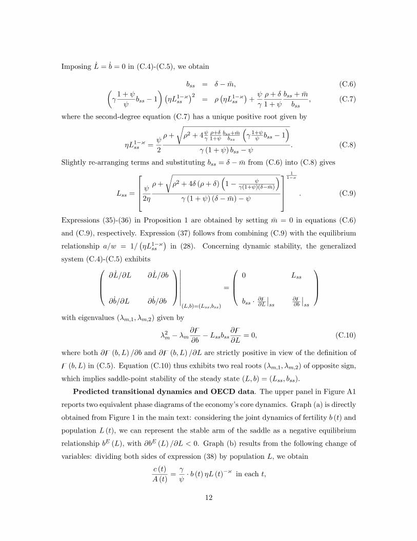
Imposing _L = _b = 0 in (C.4)-(C.5), we obtain
bss = . " ,m; (C.6))11 +
bss " 1
*=KL1%{ss
>2= -
=KL1%{ss
>+
1
-+ .
1 +
bss + ,m
bss; (C.7)
where the second-degree equation (C.7) has a unique positive root given by
KL1%{ss =
2
-+
r-2 + 4 4
#+$1+
bss+ 'mbss
11 1+ bss " 1
2
1 (1 + ) bss " : (C.8)
Slightly re-arranging terms and substituting bss = . " ,m from (C.6) into (C.8) gives
Lss =
2
664
2K
-+
r-2 + 4. (-+ .)
11"
4(1+ )($% 'm)
2
1 (1 + ) (. " ,m)"
3
775
11${
: (C.9)
Expressions (35)-(36) in Proposition 1 are obtained by setting ,m = 0 in equations (C.6)
and (C.9), respectively. Expression (37) follows from combining (C.9) with the equilibrium
relationship a=w = 1==KL1%{ss
>in (28). Concerning dynamic stability, the generalized
system (C.4)-(C.5) exhibits0
BB@
@ _L=@L @ _L=@b
@ _b=@L @ _b=@b
1
CCA
EEEEEEEE(L;b)=(Lss;bss)
=
0
BB@
0 Lss
bss $ @z@LEEss
@z@b
EEss
1
CCA
with eigenvalues (Tm;1; Tm;2) given by
T2m " Tm@z@b
" Lssbss@z@L
= 0; (C.10)
where both @z (b; L) =@b and @z (b; L) =@L are strictly positive in view of the deÖnition of
z (b; L) in (C.5). Equation (C.10) thus exhibits two real roots (Tm;1; Tm;2) of opposite sign,
which implies saddle-point stability of the steady state (L; b) = (Lss; bss).
Predicted transitional dynamics and OECD data. The upper panel in Figure A1
reports two equivalent phase diagrams of the economyís core dynamics. Graph (a) is directly
obtained from Figure 1 in the main text: considering the joint dynamics of fertility b (t) and
population L (t), we can represent the stable arm of the saddle as a negative equilibrium
relationship bE (L), with @bE (L) =@L < 0. Graph (b) results from the following change of
variables: dividing both sides of expression (38) by population L, we obtain
c (t)
A (t)=1
$ b (t) KL (t)%{ in each t,
12

which allows us to rewrite the equilibrium c=A ratio as
c=A =1
$ bE (L) $ L%{ (C.11)
where bE (L) is the saddle path appearing in the benchmark phase diagram of graph (a).
Since @bE (L) =@L < 0 for any {, and @L%{=@L < 0 for any { > 0, it follows from (C.11)
that the model predicts c (t) =A (t) to exhibit a positive relationship with the fertility rate
and, overall, a negative co-movement with L (t) regardless of whether { is zero or strictly
positive.
The lower panel of Figure A1 reports scatter diagrams in which the variables on the axes
of graph (c) and graph (d) are the empirical counterparts (in logarithmic scale) of those
on the axes of graph (a) and (b), respectively. We collected data for all OECD countries,
interpreting b as the annual crude birth rate (i.e., number of births per person) reported by
the World Bank (2017), L as total population reported by the UN (2015), c as Household
13

Final Consumption reported by OECD (2017a) divided by total population, and A with
Financial Net Worth of Households reported by OECD (2017a). The longest time series for
A available from OECD (2017a) cover the 1995-2016 period, with gaps for some countries
and no observations for Mexico and New Zealand. The overall panel dataset thus covers
the interval 1995-2016. For the sake of clarity, the scatter plots of graphs (c) and (d) in
Figure A1 refer to a sub-sample of 16 countries, namely, Chile, Estonia, France, Germany,
Great Britain, Ireland, Italy, Japan, Latvia, Luxembourg, Mexico, Portugal, Spain, The
Netherlands, Turkey, United States. Graph (c) suggests a negative within-country co-
movement between fertility rates and population size: this is conÖrmed by panel regressions
with country Öxed-e§ects computed for the whole OECD countries sample (see Table A.1,
Örst and second columns). Graph (d) similarly suggests a strong pattern of negative co-
movement between c=A and population size: this is also conÖrmed by Öxed-e§ects panel
regressions for the whole OECD countries sample (see Table A.1, third to Öfth columns).
Panel regression results, including country Öxed e§ects and additionally controlling for
country-speciÖc time trends, are reported in Table A1.
Innovation rates. The key relationships determining vertical and horizontal innova-
tion rates are the rate of return to vertical innovation (B.12) and the entry technology (22)
that we report here for simplicity,:
_Z (t)
Z (t)= D
?" 1?
pxi (t)xi (t)
zi (t)!Z (t)
w (t)+_w (t)
w (t)" r (t)" H; (C.12)
_N (t)
N (t)=
K
L (t){$ `N (t)" H: (C.13)
14

Derivation of (41). First, by symmetry, simplify Z=zi = 1 in (C.12) and rearrange terms
to get_Z (t)
Z (t)= !D
?" 1?
pxi (t)xi (t)
w (t)+_w (t)
w (t)" r (t)" H: (C.14)
Next, by symmetry, substitute pxixi =pCN from (B.17), and normalize p (t) = 1 to obtain
_Z (t)
Z (t)= !D
?" 1?
p (t)C (t)
w (t)N (t)+_w (t)
w (t)" r (t)" H = !D
?" 1?
c (t)
w (t)$L (t)
N (t)+_w (t)
w (t)" r (t)" H:
(C.15)
Next, substitute w = KA=L{ from (26) to obtain
_Z (t)
Z (t)=!D
K$?" 1?
$c (t)
a (t)$L (t){
N (t)+_w (t)
w (t)" r (t)" H: (C.16)
The growth rate of wages follows from time-di§erentiating (26): plugging
_w (t)
w (t)=
_A (t)
A (t)" {
_L (t)
L (t)(C.17)
into the right hand side of (C.16) gives
_Z (t)
Z (t)=!D
K$?" 1?
$c (t)
a (t)$L (t){
N (t)" {
_L (t)
L (t)"
"r (t)"
_A (t)
A (t)
#" H: (C.18)
From the aggregate wealth constraint (7) it follows that the term in square brackets in (C.18)
equals the excess of consumption expenditure over net labor income divided by Önancial
assets,
r (t)"_A (t)
A (t)=c (t)
a (t)" (1" 1b (t)) $
w (t)
a (t): (C.19)
Substituting (C.19) into (C.18), and rearranging terms, we have equation (41) in the main
text.
Derivation of (42). Equation (42) follows from substituting the labor market clearing
condition (24) in the entry technology (22). The derivation thus requires to consider equilib-
rium employment levels in each sector in turn. First, consider employment in intermediate
production. From (B.19), we have that `X (t) = N (t) `xi (t) may be written as
`X (t) =C (t)
Z (t)-N (t))%1+ 'N (t) ;
where we can substitute A 6EL{
6%1 = Z-N)%1 from (27) to obtain
`X (t) =?" 1
?KL (t){$C (t)
A (t)+ 'N (t)
| {z }Employment in intermediate production
(C.20)
15
Second, consider employment in vertical R&D. From the vertical innovation technology
(18), we have _Z=Z = ! $ `Z=N and, hence,
`Z (t) =1
!N (t)
_Z (t)
Z (t)| {z }Employment in vertical R&D
(C.21)
Third, using results (C.20) and (C.21), we can obtain employment in horizontal R&D
residually from the market-clearing condition (24) as
`N (t) = L (t) $ (1" 1b (t))| {z }Net labor supply
"?" 1
?KL (t){$C (t)
A (t)" 'N (t)
| {z }`X(t)
"1
!N (t)
_Z (t)
Z (t)| {z }`Z(t)
: (C.22)
Substituting (C.22) into the entry technology (22), we obtain the growth rate of the mass
of Örms (omitting time-arguments)
_N
N=
K
L{`N " H =
K
L{
"L $ (1" 1b)"
?" 1?KL{
$c
a" 'N "
1
!N_Z
Z
#" H: (C.23)
Factorizing K=L{ across the various terms in the square brackets, and recalling that KL1%{ =
w=a from (28), we obtain expression (42) in the main text.
Dynamics of the mass of Örms: preliminaries. Before proceeding, we establish
a useful result concerning the asymptotic behavior of the interest rate. From the wealth
constraint (7), the gap between the interest rate and the growth rate of Önancial wealth can
be written as in expression (C.19). In the steady state with constant population (Lss; bss),
all the terms appearing in the right hand side of (C.19) are constant (section 4.2). Since
satisfying the transversality condition (A.5) requires that r > _A=A hold in the long run,
satisfying the transversality condition (A.5) in the steady state (Lss; bss) implies
limt!1
r (t)"
_A (t)
A (t)
!=1 ca
2
ss" (1" 1bss)
1wa
2
ss> 0: (C.24)
We will exploit result (C.24) to characterize the long-run behavior of the mass of Örms.
The entry technology (22) implies that if horizontal R&D is non-operative, `N (t) = 0,
the mass of Örms declines at the obsolescence rate H and eventually reaches zero if non-
operativeness continues to hold in the long run. Therefore, a necessary condition to have
a positive mass of Örms in the long run, limt!1N (t) > 0, is that horizontal R&D is
operative, limt!1 `N (t) > 0, and that employment in entry is succiently high to guarantee
limt!1
_N (t)
N (t)= lim
t!1
K`N (t)
L (t){" H > 0: (C.25)
16

From (C.23), we can rewrite the growth rate of the mass of Örms as (eliminating time
arguments for simplicity)
_N
N=
)1"
?" 1?L2{
*$c
a"h ca"w
a(1" 1b) + H
i
| {z }r% _A
A+0
"K
L{
'+
1
!
_Z
Z
!$N (C.26)
where the term in square brackets equals r"1_A=A2+H from (C.19) and is asymptotically
strictly positive from (C.24). Combining (C.25) with (C.26), it follows that a necessary
condition to have a positive mass of Örms in the long run, limt!1N (t) > 0, is
)1"
?" 1?L2{
*$1 ca
2
ss"h1 ca
2
ss"1wa
2
ss(1" 1bss) + H
i> lim
t!1
K
L{
'+
1
!
_Z
Z
!$N; (C.27)
where the left hand side is a Önite constant and the right hand side is strictly positive
because Lss > 0, ' > 0, and _Z > 0. Expression (C.27) implies the following
Lemma 6 Any long-run equilibrium with constant population (Lss; bss) and a positive mass
of Örms limt!1N (t) > 0 exhibits a constant Önite mass of Örms Nss:
limt!1
_N (t)
N (t)= 0; lim
t!1N (t) = Nss <1:
Proof. The proof hinges on the fact that condition (C.27) can only be satisÖed as a strict
equality. The proof is by contradiction. Suppose that (C.27) holds as a strict inequal-
ity: from (C.26), the strict inequality would imply permanent growth in the mass of Örms,
limt!1_N(t)N(t) > 0, and therefore limt!1N (t) = +1, which would make the right hand side
of (C.27) grow to +1. This implies a contradiction of the hyopthesis of strict inequality
because the left hand side of (C.27) is a Önite constant. Having established that (C.27) can
only hold as a strict equality, and being (C.27) necessary to have a positive mass of Örms
in the long run, it follows that any long-run equilibrium with constant population (Lss; bss)
and a positive mass of Örms limt!1N (t) > 0 must satisfy
)1"
?" 1?L2{ss
*$1 ca
2
ss"h1 ca
2
ss"1wa
2
ss(1" 1bss) + H
i= lim
t!1
K
L{
'+
1
!
_Z
Z
!$N; (C.28)
which implies limt!1_N(t)N(t) = 0 from (C.26) and, hence, a constant Önite mass of Örms
limt!1N (t) = Nss <1 in the long run.
17
Lemma 6 suggests two remarks. The Örst remark concerns the existence of the long-
run equilibrium: since the right hand side of (C.28) is strictly positive, the existence of a
long-run equilibrium with constant population (Lss; bss) and with a positive mass of Örms
requires that the left hand side of (C.28) be strictly positive, that is,)1"
?" 1?L2{ss
*$1 ca
2
ss>1 ca
2
ss"1wa
2
ss(1" 1bss) + H
| {z }limt!1 r(t)%
_A(t)A(t)
+0
; (C.29)
where the right hand side is strictly positive by (C.24). The second remark is that (C.26)
and Lemma 6 determine a general expression for the steady-state mass of Örms
limt!1
N (t) = Nss =
11" 6%1
6L2{ss
2$=ca
>ss"F=
ca
>ss"=wa
>ss(1" 1bss) + H
G
EL{ss
='+ 1
!gssZ
> > 0; (C.30)
where gssZ % limt!1
1_Z (t) =Z (t)
2is the asymptotic rate of vertical innovations: just like
Lemma 6, expression (C.30) holds regardless of whether vertical R&D is operative, gssZ >
0, or non-operative, gssZ = 0, in the long run. In order to complete the analysis of the
interactions between horizontal and vertical innovations, it is necessary to consider the two
cases separately. We begin by discussing the case with non-operative vertical R&D, gssZ = 0.
Dynamics of the mass of Örms: non-operative vertical R&D. Suppose that
vertical R&D is non-operative in the long run, i.e., there exists a Önite instant t0 such that
_Z (t) =Z (t) = 0 in each t 2 [t0;1). In this case, expression (C.26) implies that, as long as
horizontal R&D is operative, `N (t) > 0, the mass of Örms obeys the logistic process with
time-varying coe¢cients
_N (t)
N (t)=
)1"
?" 1?L (t)2{
*$c (t)
a (t)"'c (t)
a (t)"w (t)
a (t)(1" 1b (t)) + H
(
| {z }'q1(t)
"'K
L (t){| {z }'q2(t)
$N (t) (C.31)
where both ,q1 (t) and ,q2 (t) > 0 approach Önite steady-state values, ,qss1 and ,qss2 > 0, in the
steady state with constant population (Lss; bss). If the necessary condition for the existence
of a steady state with positive mass of Örms (C.29) is satisÖed, we have ,qss1 > ,qss2 > 0, which
implies a stable steady state for the mass of Örms limt!1N (t) = Nss = ,qss1 =,qss2 ;given by
expression (C.30) with gssZ = 0.
Dynamics of the mass of Örms with operative vertical R&D / proof of Propo-
sition 2). Suppose that vertical R&D is operative in the long run, i.e., there exists a Önite
18

instant t0 such that _Z (t) =Z (t) > 0 in each t 2 [t0;1). Assuming that the steady state
with constant population (Lss; bss) and positive mass of Örms Nss > 0, the equilibrium rate
of vertical innovation (41) converges to the positive constant
limt!1
_Z (t)
Z (t)= gssZ % (1" 1bss)
1wa
2
ss+
')?" 1?
*!D
K
L{ssNss
" 1(1 c
a
2
ss" H > 0: (C.32)
The asymptotic condition for the operativess of vertical R&D is thus given by
?" 1?
!D
K
L{ssNss
1 ca
2
ss>1 ca
2
ss"1wa
2
ss(1" 1bss) + H
| {z }limt!1 r(t)%
_A(t)A(t)
+0
; (C.33)
where the right hand side is strictly positive by (C.24). Assuming that parameters are such
that the conditions for the asymptotic operativeness of horizontal and vertical R&D, (C.29)
and (C.33), are both satisÖed, the mass of Örms converges to the steady state level Nss
given by (C.30) with limt!1_Z(t)Z(t) = gssZ > 0. During the transitional interval t 2 [t1;1)
in which `N (t) > 0 and _Z (t) =Z (t) > 0, the mass of Örms obeys the logistic process with
time-varying coe¢cients
_N
N=
)1"
?" 1?L2{
*$c
a"h ca"w
a(1" 1b) + H
i
| {z }q1(t)
"K
L{
'+
1
!
_Z
Z
!
| {z }q2(t)
$N (C.34)
where both q1 (t) and q2 (t) > 0 approach Önite steady-state values, qss1 and qss2 > 0, in the
steady state with constant population (Lss; bss). If the necessary condition for the existence
of a steady state with positive mass of Örms (C.29) is satisÖed, we have qss1 > qss2 > 0 which
implies a stable steady state for the mass of Örms
limt!1
N (t) = Nss = qss1 =qss2 ; (C.35)
given by expression (C.30). We can re-express (C.34) and (C.35) in terms of the underlying
parameters as follows. From (C.34), the asymptotic values of q1 (t) and q2 (t) are given by
qss1 = limt!1
q1 (t) =1wa
2
ss(1" 1b)"
?" 1?L2{ss
$1 ca
2
ss" H; (C.36)
qss2 = limt!1
q2 (t) =K
L{ss
)'+
1
!gssZ
*: (C.37)
In equation (C.36), we substitute w=a = KL1%{ from (28) and c=a = 4 bKL
1%{ from (38)
to obtain
qss1 = limt!1
q1 (t) = (1" 1bss) KL1%{ss "?" 1?
$1
bssKL
1%3{ss " H: (C.38)
19

In equation (C.37), we substitute gssZ from (C.32) and, again, w=a = KL1%{ from (28) and
c=a = 4 bKL
1%{ from (38), to obtain
qss2 = limt!1
q2 (t) =K
L{ss
H'+
1
!
')1"
1 +
1bss
*KL1%{ss +
?" 1?
!D
1bss
LssNss
" H(I
:
(C.39)
Setting the steady state _N = 0 in (C.34), and substituting (C.38) and (C.39) in the resulting
condition qss1 = qss2 Nss, we obtain the steady-state mass of Örms
Nss =KL1%{ss
h1" 1bss "
11L2{ss
+ D2$ 6%16
4 bss
i" H
'" 1!
h(1+ )4bss%
KL1%{ss + Hi $
L{ssK: (C.40)
From (C.29) and (C.33), the same parameter restrictions guaranteeing operativeness in both
R&D activities imply that the denominator and the numerator in (C.40) are both strictly
positive. Since the numerator is increasing in Lss and the denominator is decreasing in Lss
for any { 2 [0; 1), we have dNss=dLss > 0 for any { 2 [0; 1).
D Appendix: Demographic Shocks, Income Shares and Mi-
gration
Proof of Proposition 3. The comparative-statics results with respect to bss are self-
evident: from bss = . we have dbss=d1 = 0, dbss=d- = 0, and dbss=d. > 0. The comparative-
statics results for Lss can be proved by deÖning the parameter
> % 1 (1 + ) .; (D.1)
and by rewriting the steady-state population level given by (36) as
Lss %)
K2
* 11${
2
4-+
q-2 + 4. (-+ .) .% .
>"
3
5
11${
: (D.2)
Little manipulation of the term in square brackets yields
Lss %)
K2
* 11${
2
4 -
>" +
s)-
>"
*2+4. (-+ .)
> (>" )
3
5
11${
: (D.3)
Expression (D.3) implies @Lss=@> < 0 and thereby
dLssd1
=@Lss@>
$@>
@1= (1 + ) . $
@Lss@>
< 0:
20

Since > is independent of -, expression (D.3) directly implies dLss=d- > 0. Concerning
variations in ., we have @>=@. = 1 (1 + ) > 0 but the overall sign of dLss=d. depends
on the last term inside the square root in (D.3), which is apparently ambiguous: total
di§erentiation of that last term shows that
sign@
@.
'4. (-+ .)
> (>" )
(= sign
H-+ 2.
. (-+ .)"1 (1 + )
>$2>" >"
I: (D.4)
The term in curly brackets in (D.4) can be shown to be strictly negative by contradiction:
if it were positive, we would have
-+ 2.
. (-+ .)> 1 (1 + )
>$2>" >"
; (D.5)
which, after substituting > % 1 (1 + ) . and rearranging terms, would yield
-+ 2.
-+ .> 21 (1 + ) . "
1 (1 + ) . " ;
1 +.
-+ .> 1 +
1 (1 + ) .
1 (1 + ) . " ;
.
-+ .> 1 (1 + ) .
1 (1 + ) . " :
The last inequality cannot be true since the left hand side is strictly less than unity whereas
the right hand strictly exceeds unity. This contradiction implies that (D.5) is always violated
and, hence, the term in curly brackets in (D.4) is strictly negative; this in turn implies that
the term 4$(#+$).(.% ) in expression (D.3) ñ like all the other ratios appearing inside the square
brackets ñ declines with ., so that dLss=d. < 0.
Proof of Proposition 4. The steady-state values of the three ratios considered in the
Proposition may be written as
limt!1
w (t)L (t) (1" 1b (t))A (t)
= limt!1
w (t)
a (t)(1" 1b (t)) =
1
(a=w)ss$ (1" 1bss) ; (D.6)
limt!1
C (t)
A (t)= lim
t!1
c (t)
a (t)=1 ca
2
ss=1
$
bss(a=w)ss
; (D.7)
limt!1
w (t)L (t) (1" 1b (t))C (t)
= limt!1
w(t)L(t)(1%4b(t))A(t)
C(t)A(t)
= $1" 1bss1bss
; (D.8)
where (D.7) follows from (39) and (D.8) follows from the ratio between (D.6) and (D.7).
Assuming zero migration, we can substitute in the three expressions above the steady-state
fertility rate bss = . from (35), which proves Proposition 4.
21
Derivation of (47). From (36) and (37), the wage-wealth ratio wL=A in the steady
state equals limt!1w (t)L (t) =A (t) = 1= (a=w)ss = KL1%{ss so that the signs of dd# limt!1w(t)L(t)A(t)
and dd$ limt!1
w(t)L(t)A(t) are respectively given by d
d#Lss > 0 and dd$Lss < 0, as proved in
Proposition 3.
Derivation of (48). Blanchardís (1985) model with neoclassical technology is analyzed
in depth in advanced textbooks, e.g., Barro and Sala-i-Martin (2004: Ch. 3). Consumption
per worker and assets per worker obey the dynamic system reported in Barro and Sala-
i-Martin (2004), page 183, equations [3.89]-[3.90], which can be written using our current
notation as
_a = f (a)" c" na;_c
c= f 0 (a)" -" (. + n) (-+ .)
a
c;
where a is capital per worker, f (a) is output per worker, and n is the population growth
rate. The simultaneous steady state is deÖned by the condition)f (ass)
ass" n
*=f 0 (ass)" -
>= (. + n) (-+ .) ; (D.9)
where, given positive but diminishing marginal returns to capital (that is, f 0 (a) > 0 and
f 00 (a) < 0), the left hand side is strictly decreasing in a. Therefore, exogenous increases in
- and . that increase the right hand side of (D.9) imply a lower value of steady-state capital
per worker ass,dd-ass < 0 and
dd.ass < 0: (D.10)
Since the wage rate is given by the (standard neoclassical modelís) marginal condition
w = f (a)" af 0 (a), we have
limt!1
w (t)L (t)
A (t)=f (a)" af 0 (a)
a=f (ass)
ass" f 0 (ass) ;
where the last term is strictly decreasing in ass and thus implies dd# limt!1
w(t)L(t)A(t) > 0
and dd$ limt!1
w(t)L(t)A(t) > 0 in Blanchardís (1985) model.
Migration: list of modiÖcations. Introducing migration requires modifying three
sets of expressions. First, in section 2, we need to modify (5), (11), (12), and (14). Second, in
section 4, we need to modify the expressions (29)-(34) and Proposition 1 accordingly. Third,
the expressions in Proposition 4 also require minor changes. We describe each sectionsís
modiÖcations in turn below.
22
Migration: modiÖcations to section 2. First, the demographic law (5) must be
replaced by (50) as derived above in equation (A.9). Second, equation (11) must be replaced
by_c (t)
c (t)+_p (t)
p (t)= r (t)" -"
(-+ .)
1 (1 + )
b (t) +m (t)
b (t)
a (t)
w (t); (D.11)
which is obtained by substituting pc = b1w= from (13) into the generalized equation
(A.22). Third, expression (14) must be replaced by the generalized equation (A.26). Fourth,
the augmented rate of Önancial wealth dilution appearing in (120) is simply obtained from
the last term in (D.11) above, which equals the non-augmented rate of Önancial dilution
(12) multiplied by b+mb .
Migration: modiÖcations to section 4. The dynamic system (29)-(30) must be
replaced by the generalized system given by (A.10) and (C.2), which we report here for
simplicity:
_L
L= b+m" . (D.12)
_b
b=
)11 +
b" 1
*KL1%{ " -"
1
-+ .
1 +
11 +
m
b
2 1
KL1%{+ { (b+m" .)(D.13)
where m is potentially time-varying. Note that, from (D.12)-(D.13), any simultaneous
steady state _L = _b = _m = 0 characterized by (Lss; bss;mss) must obey the general station-
arity conditions
bss = . "mss; (D.14)
Lss =
2
664
K2$-+
r-2 + 4. (-+ .)
11"
4(1+ )($%mss)
2
1 (1 + ) (. "mss)"
3
775
11${
; (D.15)
where the denominator in expression (D.15) implies that a general existence condition for
the steady state is
1 (1 + ) (. "mss) > : (D.16)
The remainder of the dynamic analysis depends on how the migration áows are speciÖed.
The next two Lemmas consider the cases of constant migration rate,m (t) = ,m, and constant
migration áows M (t) = ,M , respectively.
Lemma 7 (Steady state with constant migration rate) Assume m (t) = ,m in each instant
t. Provided that 1 (1 + ) (. " ,m) > , the simultaneous steady state (Lss; bss) of system
23
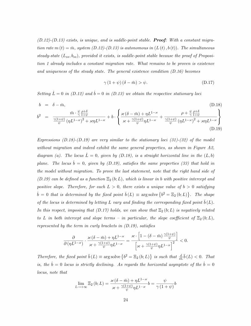
(D.12)-(D.13) exists, is unique, and is saddle-point stable. Proof: With a constant migra-
tion rate m (t) = ,m, system (D.12)-(D.13) is autonomous in (L (t) ; b (t)). The simultaneous
steady-state (Lss; bss), provided it exists, is saddle-point stable because the proof of Proposi-
tion 1 already includes a constant migration rate. What remains to be proven is existence
and uniqueness of the steady state. The general existence condition (D.16) becomes
1 (1 + ) (. " ,m) > : (D.17)
Setting _L = 0 in (D.12) and _b = 0 in (D.13) we obtain the respective stationary loci
b = . " ,m; (D.18)
b2 =,m $ 4
#+$1+
4(1+ ) (KL1%{)2 + {KL1%{
+ b $
8<
:{ (. " ,m) + KL1%{
{ + 4(1+ ) KL1%{
+-+
4#+$1+
4(1+ ) (KL1%{)2 + {KL1%{
9=
;
(D.19)
Expressions (D.18)-(D.19) are very similar to the stationary loci (31)-(32) of the model
without migration and indeed exhibit the same general properties, as shown in Figure A2,
diagram (a). The locus _L = 0, given by (D.18), is a straight horizontal line in the (L; b)
plane. The locus _b = 0, given by (D.19), satisÖes the same properties (33) that hold in
the model without migration. To prove the last statement, note that the right hand side of
(D.19) can be deÖned as a function ?2 (b;L), which is linear in b with positive intercept and
positive slope. Therefore, for each L > 0, there exists a unique value of b > 0 satisfying
_b = 0 that is determined by the Öxed point ,b (L) % arg solveOb2 = ?2 (b;L)
P. The shape
of the locus is determined by letting L vary and Önding the corresponding Öxed point ,b (L).
In this respect, imposing that (D.17) holds, we can show that ?2 (b;L) is negatively related
to L in both intercept and slope terms ñ in particular, the slope coe¢cient of ?2 (b;L),
represented by the term in curly brackets in (D.19), satisÖes
@
@ (KL1%{)${ (. " ,m) + KL1%{
{ + 4(1+ ) KL1%{
={ $h1" (. " ,m) 4(1+ )
i
h{ + 4(1+ )
KL1%{i2 < 0:
Therefore, the Öxed point ,b (L) % arg solveOb2 = ?2 (b;L)
Pis such that d
dL,b (L) < 0. That
is, the _b = 0 locus is strictly declining. As regards the horizontal asymptote of the _b = 0
locus, note that
limL!+1
?2 (b;L) ={ (. " ,m) + KL1%{
{ + 4(1+ ) KL1%{
b =
1 (1 + )b
24
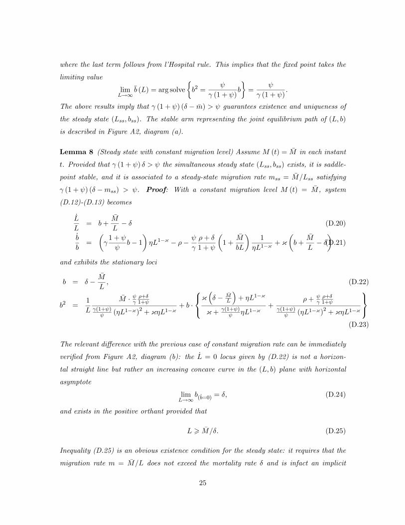
where the last term follows from líHospital rule. This implies that the Öxed point takes the
limiting value
limL!1
,b (L) = arg solve
Hb2 =
1 (1 + )b
I=
1 (1 + ):
The above results imply that 1 (1 + ) (. " ,m) > guarantees existence and uniqueness of
the steady state (Lss; bss). The stable arm representing the joint equilibrium path of (L; b)
is described in Figure A2, diagram (a).
Lemma 8 (Steady state with constant migration level) Assume M (t) = ,M in each instant
t. Provided that 1 (1 + ) . > the simultaneous steady state (Lss; bss) exists, it is saddle-
point stable, and it is associated to a steady-state migration rate mss = ,M=Lss satisfying
1 (1 + ) (. "mss) > . Proof: With a constant migration level M (t) = ,M , system
(D.12)-(D.13) becomes
_L
L= b+
,M
L" . (D.20)
_b
b=
)11 +
b" 1
*KL1%{ " -"
1
-+ .
1 +
)1 +
,M
bL
*1
KL1%{+ {
)b+
,M
L" .*(D.21)
and exhibits the stationary loci
b = . ",M
L; (D.22)
b2 =1
L
,M $ 4#+$1+
4(1+ ) (KL1%{)2 + {KL1%{
+ b $
8<
:{1. " 'M
L
2+ KL1%{
{ + 4(1+ ) KL1%{
+-+
4#+$1+
4(1+ ) (KL1%{)2 + {KL1%{
9=
;
(D.23)
The relevant di§erence with the previous case of constant migration rate can be immediately
veriÖed from Figure A2, diagram (b): the _L = 0 locus given by (D.22) is not a horizon-
tal straight line but rather an increasing concave curve in the (L; b) plane with horizontal
asymptote
limL!1
b(_b=0) = .; (D.24)
and exists in the positive orthant provided that
L > ,M=.: (D.25)
Inequality (D.25) is an obvious existence condition for the steady state: it requires that the
migration rate m = ,M=L does not exceed the mortality rate . and is infact an implicit
25
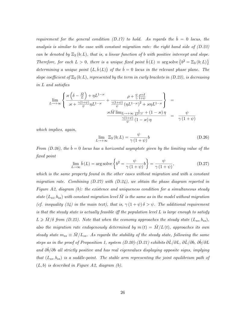
requirement for the general condition (D.17) to hold. As regards the _b = 0 locus, the
analysis is similar to the case with constant migration rate: the right hand side of (D.23)
can be denoted by ?3 (b;L), that is, a linear function of b with positive intercept and slope.
Therefore, for each L > 0, there is a unique Öxed point ,b (L) % arg solveOb2 = ?3 (b;L)
P
determining a unique point=L;,b (L)
>of the _b = 0 locus in the relevant phase plane. The
slope coe¢cient of ?3 (b;L), represented by the term in curly brackets in (D.23), is decreasing
in L and satisÖes
limL!+1
8<
:{1. " 'M
L
2+ KL1%{
{ + 4(1+ ) KL1%{
+-+
4#+$1+
4(1+ ) (KL1%{)2 + {KL1%{
9=
; =
{ ,M limL!+11
L2${+ (1" {) K
4(1+ ) (1" {) K
=
1 (1 + )
which implies, again,
limL!+1
?3 (b;L) =
1 (1 + )b (D.26)
From (D.26), the _b = 0 locus has a horizontal asymptote given by the limiting value of the
Öxed point
limL!1
,b (L) = arg solve
Hb2 =
1 (1 + )b
I=
1 (1 + ); (D.27)
which is the same property found in the other cases without migration and with a constant
migration rate. Combining (D.27) with (D.24), we obtain the phase diagram reported in
Figure A2, diagram (b): the existence and uniqueness condition for a simultaneous steady
state (Lss; bss) with constant migration level ,M is the same as in the model without migration
(cf. inequality (34) in the main text), that is, 1 (1 + ) . > . The additional requirement
is that the steady state is actually feasible i§ the population level L is large enough to satisfy
L > ,M=. from (D.25). Note that when the economy approaches the steady state (Lss; bss),
also the migration rate endogenously determined by m (t) = ,M=L (t), approaches its own
steady state mss % ,M=Lss. As regards the stability of the steady state, following the same
steps as in the proof of Proposition 1, system (D.20)-(D.21) exhibits @ _L=@L, @ _L=@b, @ _b=@L
and @ _b=@b all strictly positive and has real eigenvalues displaying opposite signs, implying
that (Lss; bss) is a saddle-point. The stable arm representing the joint equilibrium path of
(L; b) is described in Figure A2, diagram (b).
26
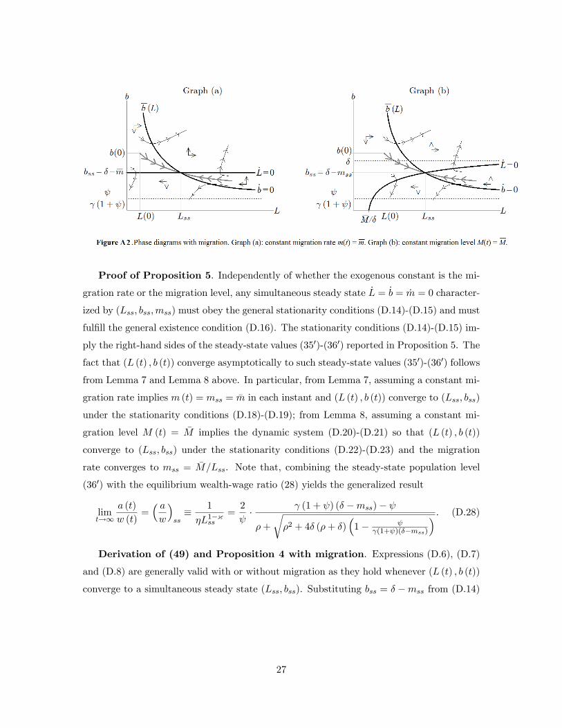
Proof of Proposition 5. Independently of whether the exogenous constant is the mi-
gration rate or the migration level, any simultaneous steady state _L = _b = _m = 0 character-
ized by (Lss; bss;mss) must obey the general stationarity conditions (D.14)-(D.15) and must
fulÖll the general existence condition (D.16). The stationarity conditions (D.14)-(D.15) im-
ply the right-hand sides of the steady-state values (350)-(360) reported in Proposition 5. The
fact that (L (t) ; b (t)) converge asymptotically to such steady-state values (350)-(360) follows
from Lemma 7 and Lemma 8 above. In particular, from Lemma 7, assuming a constant mi-
gration rate implies m (t) = mss = ,m in each instant and (L (t) ; b (t)) converge to (Lss; bss)
under the stationarity conditions (D.18)-(D.19); from Lemma 8, assuming a constant mi-
gration level M (t) = ,M implies the dynamic system (D.20)-(D.21) so that (L (t) ; b (t))
converge to (Lss; bss) under the stationarity conditions (D.22)-(D.23) and the migration
rate converges to mss = ,M=Lss. Note that, combining the steady-state population level
(360) with the equilibrium wealth-wage ratio (28) yields the generalized result
limt!1
a (t)
w (t)=1 aw
2
ss%
1
KL1%{ss=2
$
1 (1 + ) (. "mss)"
-+
r-2 + 4. (-+ .)
11"
4(1+ )($%mss)
2 : (D.28)
Derivation of (49) and Proposition 4 with migration. Expressions (D.6), (D.7)
and (D.8) are generally valid with or without migration as they hold whenever (L (t) ; b (t))
converge to a simultaneous steady state (Lss; bss). Substituting bss = . "mss from (D.14)
27

in the last terms of (D.6), (D.7) and (D.8) we obtain
limt!1
w (t)L (t) (1" 1b (t))A (t)
=1" 1 (. "mss)
(a=w)ss; (D.29)
limt!1
C (t)
A (t)= lim
t!1
c (t)
a (t)=1 ca
2
ss=1
$(. "mss)
(a=w)ss; (D.30)
limt!1
w (t)L (t) (1" 1b (t))C (t)
= limt!1
w(t)L(t)(1%4b(t))A(t)
C(t)A(t)
= $1" 1 (. "mss)
1 (. "mss); (D.31)
where the last expression (D.31) proves equation (49) in the main text. Note that, in (D.6)
and in (D.31), that long-run value (a=w)ss is given by expression (D.28) above.
E Appendix: Quantitative analysis
Calibrating the Model. The target values of endogenous variables and the values of
predetermined parameters appearing in Table 1 are calculated as follows.
Population level : the target population Lss = 36; 525; 680, matches the average population
of OECD economies in 2015 according to UN (2015) data. The set of countries is:
Australia, Austria, Belgium, Canada, Chile, Czech Republic, Denmark, Estonia, Fin-
land, France, Germany, Greece, Hungary, Iceland, Ireland, Israel, Italy, Japan, Korea,
Latvia, Luxembourg, Mexico, Netherlands, New Zealand, Norway, Poland, Portugal,
Slovak Republic, Slovenia, Spain, Sweden, Switzerland, Turkey, United Kingdom,
United States.
Consumption propensity : the target consumption propensity, c=(a+h) = 0:03, is the mid-
range value of estimated long-run propensities in large OECD countries (Boone and
Girouard, 2002) and coincides with traditional benchmark values for the US economy
(Poterba, 2000).
Consumption-assets ratio: the target value (C=A)ss = 0:64 is calculated from country-level
data (OECD, 2017a), where C is identiÖed with Household Final Consumption and
A with Financial Net Worth of Households. The longest time series for A cover the
1995-2016 period (with gaps for several countries) and are not available for Mexico
and New Zealand. We Örst calculate the average C=A ratio across OECD countries
in each year of the interval 1995-2016, obtaining 22 values ranging from 0:52 to 0:75,
and a mean value of 0:64.
28
Firms-population ratio: The target mass of Örms relative to population, Nss=Lss = 0:0327,
is calculated as follows. First, we calculate the aggregate number of entreprises in
2013 in OECD economies by summing across countries the data reported in OECD
(2016a: Ch.2, Table 2.1) obtaining 46; 060; 568 Örms (all sizes and sectors). Dividing
this number by 39 countries, we obtain the OECD average number of Örms Nss =
1; 181; 040, which can be divided by the OECD average population Lss = 36; 525; 680
to obtain Nss=Lss = 0:0327.
Long-term growth. The target growth rate of Önal output ( _A=A)ss = 0:014 is computed
from the long-term GDP forecasts published in OECD (2014a). According to these
predictions, the OECD-average real growth rate will converge to 1.4% in year 2060.
R&D propensity. The target value of R&D propensity, 0:022, is the 1995-2015 average of
the time series of R&D expenditures-to-GDP in OECD countries reported in OECD
(2017b).
Expected adult lifetime. Data from OECD-Stat (2016) for the year 2016 imply an average
life expectancy at birth across OECD countries equal to 79.5 years. Since o¢cial
working-age typically starts between 16 and 18 years, we subtract 17 years to life
expectancy at birth, obtaining the average adult lifetime 62:5 that we use in setting
the value of 1=..
Net immigration rate. The reference value mss = 0:23% is obtained from OECD (2017c)
data reporting 5-year net immigration levels for each country over the 1973-2012
period. We build for each country the estimated yearly net ináows within each 5-
year period (as the mean value between consecutive 5-year observations) and then
divide the obtained numbers by population in the same year to obtain estimated
yearly net immigration rates. We then compute the average net immigration rate for
each country over the 1973-2012 period, and then calculate the average across OECD
coutries obtaining mss = 0:23%.
Elasticity of substitution across intermediates. The reference value ? = 4:3 is chosen so as to
generate in the model an equilibrium mark-up for monopolistic Örms ?= (?" 1) = 1:3,
which is in the middle of the range 1:2-1:4 suggested by most estimates of economy-
wide mark-ups for the US and UK economies ñ see Britton et al. (2000), Gali et al.
29
(2007) ñ and is consistent with OECD estimates by Oliveira Martins et al. (1996).
Gains from variety. As noted in the main text, most of the evidence on the ëgains from
variety expansioní comes from empirical studies of international trade. A major rea-
son is that trade data contain detailed records of goods characteristics with highly
disaggregated industrial classiÖcations, so that data on internationally traded goods
are much more granular than data on goods that are produced and sold domesti-
cally. This however implies that the empirical estimates of gains from variety are
not fully consistent with the notion of ëgains from varietyí typically considered in
growth-theoretic models ñ i.e., the ëgains from di§erentiationí originally emphasized
by Romer (1990). A Örst problem is that most econometric models of trade identify
the gains from variety with a ëlove-for-varietyí parameter that appears in consumers
preferences (Spence, 1976; Dixit and Stiglitz, 1977) whereas our theoretical model
follows the standard growth-theoretic speciÖcation (Ethier, 1982; Romer, 1990) that
identiÖes such gains from variety with a technology parameter. A second problem is
that most econometric models of trade estimate static gains from variety by treating
all traded goods as Önal goods consumed by households: in reality, a large share of
traded goods consists of intermediate inputs/capital goods and this implies that the
actual gains from variety should include non-negligible dynamics gains that are how-
ever neglected in empirical studies. A third problem is that studies of trade typically
concentrate on the welfare gains that an economy enjoys as a result of increases in
the mass of imported varieties: if there exists a non-negligible di§erence between the
number of varieties that a country imports from abroad and the number of varieties
that the country produces and sells domestically, the overall ëgains from variety expan-
sioní that an economy enjoys may substantially di§er from the gains from imported
varieties. The three problems mentioned above suggest a áexible parametrization of
@ " 1, the elasticity of productivity to the mass of intermediate goods. The closest
empirical counterpart to our @" 1 is the ëelasticity of productivity to varietyí calcu-
lated by Broda et al. (2006), which ranges from 0:05 to 0:20. We adopt the baseline
value @ " 1 = 0:05 and subsequently check the sensitivity of our results to imposing
the alternative values 0:10-0:15.
30
Appendix: References
Barro, R., Sala-i-Martin, X. (2004). Economic Growth. MIT Press.
Blanchard, O. (1985). Debt, DeÖcits, and Finite Horizons. Journal of Political Economy
93: 223-247.
Boone, L., Girouard, N. (2002). The stock market, the housing market and consumer
behaviour. OECD Economic Studies 35, 2002/2.
Britton, E., Larsen, J., Small, I. (2000). Imperfect competition and the dynamics of
markups. Bank of England working papers 110, Bank of England.
Broda, C., GreenÖeld, J., Weinstein, D. (2006). From Groundnuts to Globalization: A
Structural Estimate of Trade and Growth. NBER Working Papers 12512, National
Bureau of Economic Research.
Dixit, A., Stiglitz, J. (1977). Monopolistic Competition and Optimum Product Diversity.
American Economic Review 67 (3): 297-308.
Ethier, W. (1982). National and International Returns to Scale in the Modern Theory of
International Trade. American Economic Review 72 (3): 389-405.
Gali, J., Gertler, M., LÛpez-Salido, J.D. (2007). Markups, Gaps, and the Welfare Costs of
Business Fluctuations. Review of Economics and Statistics 89 (1): 44-59.
OECD (2014a). Economic Outlook No 95 - May 2014, www.stats.oecd.org (dataset ac-
cessed July 2017). Organisation for Economic Co-operation and Development.
OECD (2016a). Entrepreneurship at a Glance 2016. Organisation for Economic Co-
operation and Development.
OECD (2017a). National Accounts at a Glance 2017, www.stats.oecd.org (dataset accessed
July 2017). Organisation for Economic Co-operation and Development.
OECD (2017b). Research and Development Statistics 2017, www.stats.oecd.org (dataset
accessed July 2017). Organisation for Economic Co-operation and Development.
OECD (2017c). World Development Indicators, www.stats.oecd.org (dataset accessed July
2017). Organisation for Economic Co-operation and Development.
31
Oliveira Martins, J., Scarpetta, S., Pilat, D. (1996). Mark-up pricing, market structure
and the business cycle. OECD Economic Studies 27, 1996/II.
Poterba, J.M. (2000). Stock Market Wealth and Consumption. Journal of Economic
Perspectives 14 (2): 99ñ118.
Romer, P. (1986). Increasing Returns and Long-run Growth. Journal of Political Economy
94 (5): 1002-1037.
Romer, P. (1990). Endogenous Technological Change. Journal of Political Economy 98
(5): 71-102.
Spence, M. (1976). Product Di§erentiation and Welfare. American Economic Review 66
(2): 407-414.
UN (2015). World Population Prospects: The 2015 Revision, DVD Edition. United Na-
tions, Department of Economic and Social A§airs, Population Division.
World Bank (2017). Databank ñ crude brith rates, downloaded from https://data.worldbank.org
(dataset accessed July 2017).
32
Related Documents