WAVELET BASED DECONVOLUTION TECHNIQUES IN …etd.lib.metu.edu.tr/upload/12613870/index.pdf · submitted by EMİNE ADLI YILMAZ in partial fulfillment of the requirements for ... Performance

WAVELET BASED DECONVOLUTION TECHNIQUES IN IDENTIFYING

FMRI BASED BRAIN ACTIVATION

A THESIS SUBMITTED TO

THE GRADUATE SCHOOL OF NATURAL AND APPLIED SCIENCES

OF

MIDDLE EAST TECHNICAL UNIVERSITY

BY

EMİNE ADLI YILMAZ

IN PARTIAL FULFILLMENT OF THE REQUIREMENTS

FOR

THE DEGREE OF MASTER OF SCIENCE

IN

ELECTRICAL AND ELECTRONICS ENGINEERING

SEPTEMBER 2011

Approval of the thesis:



submitted by EMİNE ADLI YILMAZ in partial fulfillment of the requirements for the degree of Master of Science in Electrical and Electronics Engineering Department, Middle East Technical University by,

Prof. Dr. Canan Özgen ___________ Dean, Graduate School of Natural and Applied Sciences Prof. Dr. İsmet Erkmen ___________ Head of Department, Electrical and Electronics Engineering Prof. Dr. Aydan Erkmen ___________ Supervisor, Electrical and Electronics Engineering Dept.,METU Assist. Prof.Dr. Didem Gökçay ___________ Co-supervisor, Informatics Institute, METU

Examining Committee Members:

Prof. Dr. Mustafa Kuzuoğlu ___________ Electrical and Electronics Engineering Dept.,METU

Prof. Dr. Aydan Erkmen ___________ Electrical and Electronics Engineering Dept.,METU

Assist. Prof.Dr. Didem Gökçay ___________ Informatics Institute, METU

Assist. Prof. Dr. Yesim Serinagaoglu ___________ Electrical and Electronics Engineering Dept.,METU

Assist. Prof.Dr. Mustafa Doğan ___________ Control Engineering Dept., Doğuş University

Date: ___________

I hereby declare that all information in this document has been obtained and

presented in accordance with academic rules and ethical conduct. I also declare

that, as required by these rules and conduct, I have fully cited and referenced

all material and results that are not original to this work

Name, Last name: Emine Adlı Yılmaz

Signiture:

iii

iv

ABSTRACT



Adlı Yılmaz, Emine

M.S. Department of Electrical and Electronics Engineering

Supervisor : Prof.Dr. Aydan Erkmen

Co-supervisor : Assist. Prof.Dr. Didem Gökçay

September 2011, 171 pages

Functional Magnetic Resonance Imaging (fMRI) is one of the most popular

neuroimaging methods for investigating the activity of the human brain during

cognitive tasks. The main objective of the thesis is to identify this underlying brain

activation over time, using fMRI signal by detecting active and passive voxels. We

performed two sub goals sequentially in order to realize the main objective. First, by

using simple, data-driven Fourier Wavelet Regularized Deconvolution (ForWaRD)

method, we extracted hemodynamic response function (HRF) which is the

information that shows either a voxel is active or passive from fMRI signal. Second,

the extracted HRFs of voxels are classified as active and passive using Laplacian

Eigenmaps. By this, the active and passive voxels in the brain are identified, and so

are the activation areas.

The ForWaRD method is directly applied to fMRI signals for the first time. The

extraction method is tested on simulated and real block design fMRI signals,

contaminated with noise from a time series of real MR images. The output of

ForWaRD contains the HRF for each voxel. After HRF extraction, using Laplacian

Eigenmaps algorithm, active and passive voxels are classified according to their

HRFs. Also with this study, Laplacian Eigenmaps are used for HRF clustering for the

first time. With the parameters used in this thesis, the extraction and clustering

methods presented here are found to be robust to changes in signal properties.

v

Performance analyses of the underlying methods are explained in terms of sensitivity

and specificity metrics. These measurements prove the strength of our presented

methods against different kinds of noises and changing signal properties.

Keywords: Hemodynamic response function (HRF) extraction, classification of

HRFs, Functional Magnetic Resonance Imaging, fMRI

vi

ÖZ

Yüksek Lisans, Department of Electrical and Electronics Engineering

Tez Yöneticisi : Prof.Dr. Aydan Erkmen

Ortak Tez Yöneticisi : Assist. Prof.Dr. Didem Gökçay

Eylül 2011, 171 sayfa

Fonksiyonel Manyetik Rezonans Görüntüleme (fMRG), beynin aktivasyon sürecini

araştırmada kullanılan en yaygın yöntemlerinden biridir. Bizim tez çalışmamızın

temel amacı, fMRG sinyallerini kullanarak, beyindeki aktif ve pasif vokselleri

saptayıp, zamana bağlı olan beyin aktivasyonunu belirlemektir. Bu hedefe ulaşmak

için sırasıyla iki adet ön hedefi gerçekleştirdik. İlk olarak, basit ve veritabanlı bir

yöntem olan Fourier ve Wavelet Alanlarında Regülarizasyonlu Ters Konvolusyon

(ForWaRD) metodunu kullanarak fMRG sinyalinden, bir vokselin aktif ya da pasif

olduğunu gösteren bilgiyi, yani hemodinamik cevap fonksiyonunu (HCF) elde ettik.

Daha sonra, Laplacian Özharitalama yöntemini kullanarak, elde ettiğimiz

hemodinamik cevap fonksiyonlarını aktif ve pasif olma durumlarına bakarak

sınıflandırdık. Bu sayede hem beyindeki aktif ve pasif vokseller hem de aktivasyon

bölgeleri bulunmuş oldu.

Bu tez çalışması ile birlikte ForWaRD yöntemi ilk kez fMRG sinyallerine doğrudan

uygulanmıştır. Çıkarım yöntemi, üzerine gerçek MR gürültüleri eklenmiş, gerçek ve

benzetimi yapılmış blok tasarım aktivasyon sinyallerinde test edilmiştir. ForWaRD

işleminin çıkışı her bir voksel için HCF içermektedir. HCF çıkarımından sonra

Laplacian Özharitalama yöntemi kullanılarak, aktif ve pasif vokseller HCF'lerine

göre sınıflandırılmışlardır. Bu çalışma ile ayrıca Laplacian Özharitalama yöntemi ilk

defa HCF sınıflandırmada kullanılmıştır.

Mevcut parametreler ile bu tezde uygulanan çıkarım ve sınıflandırma yöntemlerinin,

sinyal özelliklerindeki değişimlere karşı çok dirençli oldukları görülmüştür. Bahsi

geçen yöntemlerin verim analizleri, hassaslık ve belirlilik yönlerinden incelenmiş ve

açıklanmıştır. Bu ölçümler de sunduğumuz metotların farklı gürültü tiplerine ve

sinyale özelliklerindeki değişikliklere karşı ne kadar güçlü olduğunu kanıtlamıştır.

vii

Anahtar kelimeler: Hemodinamik cevap fonksiyonu (HCF) çıkarımı, HCF

sınıflandırılması, Fonksiyonel Manyetik Rezonans Görüntüleme Analizi, fMRG.

viii

ACKNOWLEDGEMENTS

This thesis could not have been written without my love Akın YILMAZ who not

only supported but also encouraged and helped me throughout my academic

program.

Also, I would like to give special thanks to my thesis supervisor, Prof. Dr. Aydan

ERKMEN and my co-supervisor, Assoc. Prof. Dr. Didem GÖKÇAY for their

professional support, guidance and encouragements which were invaluable for me

during this thesis’ preparation.

And my deepest gratitude to my parents and Gamze Laitila in supporting and helping

me.

Lastly, I want to thank Ulas Ciftcioglu, Mete Balci and Serdar Baltaci for all their

help, support and valuable hints.

ix

TABLE OF CONTENTS

ABSTRACT ................................................................................................................ iv

ÖZ ............................................................................................................................... vi

TABLE OF CONTENTS ............................................................................................ ix

LIST OF TABLES ...................................................................................................... xi

LIST OF FIGURES ................................................................................................... xii

CHAPTERS

1 INTRODUCTION ............................................................................................... 1

1.1 Thesis Objective and Goals ........................................................................... 4

1.1.1 Goal 1: Extraction of Hemodynamic Response from fMRI Signal ....... 4

1.1.2 Goal 2: Classification of voxels as active and passive ........................... 9

1.2 Methodology ............................................................................................... 10

1.3 Contribution ................................................................................................. 14

1.4 Outline of the Thesis ................................................................................... 15

2 LITERATURE SURVEY and MATHEMATICAL BACKGROUND ............. 16

2.1 The fMRI time series and Pre-Processing Steps ......................................... 17

2.1.1 Principal Component Analysis of fMRI Data ...................................... 17

2.1.2 Independent Component Analysis (ICA) of fMRI Data ...................... 19

2.2 Data-driven approaches for fMRI analysis.................................................. 20

2.3 Model-driven approaches for fMRI analysis based on wavelets................. 21

2.4 Clustering of FMRI data .............................................................................. 23

2.5 Mathematical Background........................................................................... 26

2.5.1 Deconvolution ...................................................................................... 26

2.5.2 Clustering of Hemodynamic responses as active and passive ............. 46

3 METHOD ........................................................................................................... 49

3.1 How ForWaRD is Adapted for Hemodynamic Response Function Extraction ............................................................................................................... 50

3.1.1 Determining the HRF ........................................................................... 51

3.1.2 Regularization ...................................................................................... 54

3.1.3 Using ForWaRD to obtain the HRF ..................................................... 59

3.2 Clustering .................................................................................................... 65

x

3.2.1 Clustering of FMRI data ...................................................................... 65

3.2.2 Clustering Algorithm Outline .............................................................. 65

4 EXPERIMENT RESULTS AND DISCUSSIONS ............................................ 72

4.1 Experimental Design Types ........................................................................ 72

4.1.1 Block design paradigm ......................................................................... 72

4.1.2 Event-related design paradigm ............................................................. 73

4.2 Experiment Results ...................................................................................... 74

4.2.1 Results of Extracted HRF with ForWaRD Algorithm ......................... 75

4.2.2 Clustering Results and Identification of Active and Passive Voxels . 112

5 SENSITIVITY AND PERFORMANCE ANALYSIS .................................... 124

5.1 Sensitivity and Performance Analysis ....................................................... 124

5.1.1 Sensitivity and Performance Analysis of ForWaRD method According to The Changing System Parameters. .............................................................. 126

5.1.2 Sensitivity and Performance Analysis of Fuzzy C means Clustering Method According to The Changing System Parameters ................................ 144

6 DISCUSSIONS ................................................................................................ 148

6.1 Performance Comparison of ForWaRD and Blind Deconvolution ........... 148

6.1.1 ForWaRD and Blind Deconvolution .................................................. 148

6.1.2 RESULTS .......................................................................................... 150

6.1.3 CONCLUSIONS ................................................................................ 156

6.2 Enhancing the Extracted Hemodynamic Response Results for ForWaRD using a Blind Deconvolution Method .................................................................. 157

CONCLUSION ........................................................................................................ 160

REFERENCES ......................................................................................................... 163

xi

LIST OF TABLES

Table 1 MSE values between estimated and ıdeal fMRI ............................................ 96 Table 2 Sensitivity and Specificity values for clustering results of data on which only AWGN noise added ................................................................................................. 115 Table 3 Sensitivity and Specificity values results for clustering of data on which varying values of AWGN, jitter, drift, lag ............................................................... 117 Table 4 Sensitivity and Specifity Analysis for Variable σAWGN ................................. 118 Table 5 Sensitivity and Specifity Analysis for Variable σJitter ................................... 119 Table 6 Sensitivity and Specifity Analysis for Variable σDrift ................................... 119 Table 7 Sensitivity and Specifity Analysis for Variable σLag .................................... 120 Table 8 Sensitivity and Specifity Analysis for Variable σLag, σDrift, σAWGN and σJitter . 120 Table 9 MSE comparison for varying Tikhonov regularization parameter τ .......... 129 Table 10 MSE comparison for varying Wiener regularization parameter α ........... 129 Table 11 MSE comparison for variable Threshold Factor µ while decomposition level is fixed at 4 ....................................................................................................... 136 Table 12 Specificity and Sensitivity analysis for variable threshold factor µ ......... 137 Table 13 MSE comparison with respect to variable Decomposition levels with Soft and Hard Thresholds ............................................................................................... 139 Table 14 Sensitivity and Specificity analysis for variable decomposition level n with fixed threshold factor µ ............................................................................................ 142 Table 15-Sensitivity and Specificity analyses with respect to Euclidean Dist. and Nearest Neighbor ..................................................................................................... 146 Table 16 Sensitivity and Specificity analyses with respect to Cosine Distance and Nearest Neighbor ..................................................................................................... 146 Table 17 The effect of different noises on the clustering results of both methods ... 153 Table 18 Clustering results under combined noise and lag-drift conditions ........... 154

xii

LIST OF FIGURES

Figure1.1 The recorded hemodynamic response signal (solid line) triggered by a single event (dashed line)[37] ...................................................................................... 6 Figure1.2 On the left, active voxel’s hemodynamic response waveform of the right is the one for a passive voxel. .......................................................................................... 6 Figure1.3 FMRI signal without noise [21] .................................................................. 7 Figure1.4-FMRI signal with noise [21] ....................................................................... 7 Figure1.5 Left: Shape of a fundamental wavelet function called Mexican Hat. Right: ideal shape of the hemodynamic response in fMRI to a single stimulus. The four stages of the hemodynamic response are: A: lag-on; B: rise; C: decay; D: dip ....... 10 Figure1.6 Examples of mother wavelets: (a) Daubechies family (b) Coiflets family (c) Symlet family .............................................................................................................. 11

Figure2.1 A system that performs deconvolution separates two convolved signals .. 26 Figure2.2 Undesired convolution and structure of deconvolution [9] ...................... 27 Figure2.3 Wavelet Based Regularized Deconvolution (WaRD) [93] ........................ 30 Figure2.4 Fourier-wavelet regularized deconvolution ( ForWaRD ) process steps[21] ..................................................................................................................... 32 Figure2.5 Bank of filters for deconvolution of signal x(t), which is distorted by the instrument function H(t), with a three-stage scheme of DWT: y(n) are samples of the observed signal; =γ(−k), =h(-k) and ḡ =g(–k) are the coefficients of the filters for analysis; γ, h, and g are the coefficients of the filters for synthesis; and f(t) is the reconstructing function.[9] ........................................................................................ 35 Figure2. 6 Reconstructed signal from an observation for capillary electrophoresis: (a) observed signal y(t) and (b) signal processed in accordance with the wavelet-based deconvolution ..................................................................................... 38 Figure2.7 Convolution model setup. .......................................................................... 38 Figure2.8 Process steps of Fourier-wavelet regularized deconvolution (ForWaRD) 42

Figure3.1 System Diagram of the Thesis.................................................................... 49 Figure3. 2 Example of a block design stimulus pattern and its Fourier transform ... 53 Figure3.3 Block Diagram of ForWaRD ..................................................................... 53 Figure3.4 fMRI signal. ............................................................................................... 61 Figure3.5 Output of Fourier inversion step .............................................................. 62 Figure3.6 Deconvolved HRF After Fourier Shrinkage .............................................. 63 Figure3.7 ForWaRD - Extract deconvolved and denoised HRF from fMRI signal ... 64

Figure4.1 Example of a block design stimulus pattern .............................................. 72

xiii

Figure4.2 Example of a event-related design stimulus pattern .................................. 73 Figure4.3 Stimulus pattern and simulated pure fMRI signal, called ideal BOLD response ..................................................................................................................... 76 Figure4.4 Hemodynamic Response Extraction steps. ................................................ 79 Figure4.5 Extracted Hemodynamic Response ............................................................ 80 Figure4. 6 Ideal hemodynamic response shape ......................................................... 80 Figure4.7 Similarity Between The Estimated BOLD and Ideal BOLD ...................... 81 Figure4.8 Hemodynamic Response Extraction steps. ................................................ 82 Figure4.9 Extracted Hemodynamic Response ............................................................ 83 Figure4.10 Similarity Between The Estimated BOLD and Ideal BOLD .................... 84 Figure4.11 Hemodynamic Response Extraction steps. .............................................. 85 Figure4.12 Extracted Hemodynamic Response.......................................................... 86 Figure4.13 Similarity between The Estimated BOLD and Ideal BOLD .................... 87 Figure4.14 Hemodynamic Response Extraction steps. .............................................. 88 Figure4.15 Extracted Hemodynamic Response.......................................................... 88 Figure4.16 Similarity Between The Estimated BOLD and Ideal BOLD .................... 89 Figure4.17 Hemodynamic Response Extraction steps. .............................................. 90 Figure4.18 Extracted Hemodynamic Response.......................................................... 91 Figure4.19 Similarity Between The Estimated BOLD and Ideal BOLD .................... 91 Figure4.20 Hemodynamic Response Extraction steps. .............................................. 92 Figure4. 21 Extracted Hemodynamic Response......................................................... 93 Figure4. 22 Similarity Between The Estimated BOLD and Ideal BOLD ................... 94 Figure4.23 Hemodynamic Response Extraction steps. .............................................. 95 Figure4.24 Simulated Passive fMRI Data .................................................................. 96 Figure4.25: Hemodynamic response signal of passive data ...................................... 97 Figure4.26 Extracted Hemodynamic Response Function for a Passive Simulated Data ............................................................................................................................ 97 Figure4.27 Stimulus pattern of Fingertapping Experiment........................................ 98 Figure4.28 Observed Real active Finger-tapping data.............................................. 99 Figure4.29 ForWARD steps for HRF extraction........................................................ 99 Figure4.30 Extracted HRF for active fMRI data ..................................................... 100 Figure4.31 Observed Real passive Finger-tapping data ......................................... 101 Figure4.32 Extracted passive signal ........................................................................ 101 Figure4.33 Stimulus pattern of the experiment ........................................................ 103 Figure4.34 Ideal HRF(a) & Ideal fMRI (b) ............................................................. 104 Figure4. 35–Active and Passive vozel locations in the brain .................................. 105 Figure4.36 a) Original real fMRI data and b) normalized version of the underlying one ............................................................................................................................ 106 Figure4.37 Extracted Hemodynamic Response........................................................ 106 Figure4.38 Comparison of ideal and estimated BOLD change ............................... 107 Figure4.39 Original real fMRI data and normalized version of the underlying one108 Figure4.40 Extracted Hemodynamic Response........................................................ 109 Figure4.41 Comparison of ideal and estimated BOLD change ............................... 109

xiv

Figure4.42 Original passive fMRI signal ................................................................. 110 Figure4.43 ForWARD output of passive fMRI data ................................................. 110 Figure4.44 Original motion fMRI data .................................................................... 111 Figure4.45 ForWARD output of motion fMRI data ................................................. 111 Figure4.46 Cluster results for noisy simulated fMRI data which has AWGN σ=4 .. 112 Figure4. 47 Cluster results for noisy simulated fMRI data which has AWGN σ=16 .................................................................................................................................. 113 Figure4.48 Cluster results for noisy simulated fMRI data which has AWGN σ=30 114 Figure4.49 Clusters of fingertapping data ............................................................... 121 Figure4.50 Clusters of fMR adaptation paradigm ................................................... 123

Figure5.1 Noisy Simulated Data .............................................................................. 125 Figure5.2 Stimulus pattern and pure simulated fMRI signal ................................... 125 Figure5.3 Process steps of Fourier-wavelet regularized deconvolution (ForWaRD)[21] ....................................................................................................... 126 Figure5.4 MSE plot versus varying Tikhonov regularization parameter τ .............. 129 Figure5. 5 MSE plot versus varying Wiener regularization parameter α ................ 130 Figure5.6 Extracted HRF for Threshold Factor value μ=20 ................................... 135 Figure5.7 MSE versus Threshold Factor µ .............................................................. 136 Figure5.8 MSE versus Decomposition Level n with Soft & Hard Thresholding ..... 139 Figure5.9 The best extracted HRF result for data we used in Chapter 5 ................ 143 Figure5.10 Clustering Result, Euclidean, 4NN ........................................................ 145 Figure5.11 Clustering Result, Euclidean, 6NN ........................................................ 145 Figure5.12 Clustering Result, Cosine, 6NN ............................................................. 145

Figure6.1 Estimated HRF and stimulus pattern via MAP Blind Deconvolution using simulated data .......................................................................................................... 151 Figure6.2 Estimated HRF and stimulus pattern via FORWARD using simulated data .................................................................................................................................. 151 Figure6.3 Estimated HRF and stimulus pattern via MAP Blind Deconvolution using real fMRI data .......................................................................................................... 152 Figure6.4 Estimated HRF and stimulus pattern via FORWARD using real fMRI data .................................................................................................................................. 152 Figure6. 5 The illustration of clustering with the simulated data parameters σ_AWGN = 4; σ_Jitter=4 σ_Drift = 16; σ_Lag = 16 using Blind Deconvolution .. 154 Figure6.6 The illustration of clustering with the simulated data parameters σ_AWGN = 4; σ_Jitter=4 ......................................................................................................... 155 Figure6.7 Clustering of real fMRI data via Method1 .............................................. 155 Figure6.8 Clustering of real fMRI data via Method2 .............................................. 156 Figure6. 9 HRF Results for Ideal and Estimated Stimulus Patterns ........................ 158

xv

to Akın who is my everything

1

CHAPTER 1

INTRODUCTION

1 INTRODUCTION

The main objective of this thesis is to identify brain activation over time by detecting

active and passive voxels using the FMRI signal at a specific period of time, the

smallest three dimensional unit that spans the grid based three dimensional

representation of the brain volume being a voxel.

When people are involved in a task, a process or an emotion, only the voxels that are

related to these actions become active and others remain passive. On the other hand,

some voxels are affected by head movement, causing the assoociated time series to

contain motion artifacts. A set of voxels participating in processing a specific task,

process or emotion are present in different parts of the brain. If voxels containing

active processing, passive noise and motion artifacts, as well as their locations in the

brain can be identified, then we will be able to predict the functionality of that part of

the brain.

In order to detect and analyze brain activation, we must first obtain functional data

from the brain. In the literature, there are many techniques to obtain data from brain

using brain imaging techniques: Computed tomography (CT), developed in 1970s

being one of the earliest imaging techniques. In order to constitute cross-sectional

images of the brain, computed tomography scanning method uses X-rays. When a

patient goes through a CT scan, X-ray images of the brain are taken with rings that

circle around the patient’s head. CT scans efficiently map out the gross features of

the brain, but lack the ability to give a true representation of the brain function [85].

Electroencephalography, shortly EEG, is a test method to measure the amount of

electrical activity in the brain using electrodes. EEG is often used in

2

experimentation because it is non-invasive for the patient. It is notably sensitive and

is capable of tracking changes in electrical activity milliseconds after neuronal

activity [86]. Magnetoencephalography (MEG), measures the magnetic fields which

come from the electrical brain activity. These magnetic fields are called SQUIDS

and the devices that are used in MEG are greatly sensitive in detecting them [87].

Another method for measuring blood oxygenation in the brain is an optical technique

called NIRS. Light in the near infrared part of the spectrum (700-900nm) is sent

through the skull and reemerging light is detected. This measuring depends on

attenuation of the traveling light which is correlated with blood oxygenation.

Therefore NIRS can provide an indirect measure of brain activity. [88].

In recent papers, Magnetic Resonance Imaging (MRI) method is often investigated in

the brain imaging. An anatomical view of the brain (not functional) is what exactly

MRI shows (not functional). It detects radio frequency signals. In the MRI

procedure, no radioactive materials or X-rays are used and this feature is its major

advantage. [89]

Other methods in the literature specifically measure the brain activity. One of them is

Positron Emission Tomography, or shortly PET scan. PET scan uses short-lived

radioactive material’s minuscule amount that is either injected or inhaled and detects

functional processes in the brain. The radioactive material includes nitrogen, oxygen,

carbon and fluorine. While this material travels through the bloodstream, the oxygen

and glucose accumulate in the metabolically active areas of the brain. When this

radioactive material starts to break down, neutrons and positrons are produced. When

neutron and positron clash, gamma rays are released. This is what creates the image

of the brain. Another technique is functional magnetic resonance imaging, fMRI, that

does not need radioactive materials. In addition, it produces images at a higher

resolution than PET. Since the early 1990s, fMRI's relatively wide availability, low

invasiveness and absence of radiation exposure have let it dominate the brain

mapping field. Functional MRI (fMRI) is a brain imaging technique based on MR-

imaging. Functional MRI (fMRI) is a brain imaging technique based on MR-

imaging. This technique is used to measure brain activity by

3

monitoring the increase in blood oxygenation and blood flow, which indicates the

areas of the brain that are most active. fMRI allows us to view both an anatomical

and a functional image of the brain.

Functional MRI does not need radioactive materials when detecting functional

processes in the brain while producing brain images at a higher resolution than the

other methods. This important feature encourages us to use fMRI method for

obtaining functional data from the brain which is used for identifying functional

structure of brain in our thesis.

fMRI has advantages and disadvantages like any other technique. The experiments

must be carefully designed and conducted to maximize its strengths and minimize its

weaknesses in order to be useful. Some important advantages of fMRI are the

following: First, it can noninvasively record brain signals without risks of radiation

implicit in other scanning methods, such as CT or PET scans. Second, it has high

spatial resolution. Third, signals coming from all regions of the brain can be recorded

with fMRI. Finally, fMRI produces compelling images of brain "activation". In

addition to these positive features it has some disadvantages too. Being highly

sensitive to the motion and having limited temporal resolution are the most important

disadvantages. fMRI technique outputs a blood oxygenation level dependent signal

(BOLD). A variety of factors, including: brain pathology, drugs/substances, age,

attention etc. can effect this signal. And since it is a very complex signal, we have to

perform many computations to identify activation areas. Since the advantages

outweigh disadvantages, for determining the activation region for a specific task in a

predetermined time, we will process data collected by fMRI.

4

1.1 Thesis Objective and Goals

The basic aim of our work is to detect voxel based activation in the brain based on

processing fMRI signals.

We have to execute two sub goals sequentially in order to realize the main objective.

First goal is to estimate information about each voxel’s activity and passivity from

the fMRI signal and this information is called hemodynamic response. All voxels in

the brain have a hemodynamic response function and when these responses are

estimated and analyzed we can detect active participation of the voxels based on the

shape of the hemodynamic response. The first sub goal of the thesis includes

hemodynamic response extraction. The second sub goal encompasses analyses of the

estimated hemodynamic responses according to their features yielding classification

of these features as generated from active versus passive voxels. These subgoals are

explained in detail below.

1.1.1 Goal 1: Extraction of Hemodynamic Response from fMRI Signal

1.1.1.1 What is fMRI and Hemodynamic Response?

Functional MRI (fMRI) is an MRI-based brain imaging technique which allows us

to detect the brain areas which are involved in a process, a task or an emotion. This

means that we use fMRI to monitor the brain activity. We can use standard MRI

scanners since this brain imaging technique is a type of specialized MRI scan.

fMRI works by detecting the changes in blood oxygenation and flow that occur in

response to neural activity. When brain voxels are activated, they consume more

oxygen. To meet this underlying increased demand, blood flow increases towards the

active brain area. Oxygen is delivered to neurons by hemoglobin. This means when

neural activity increases, hemoglobin with oxygen called oxyhemoglobin increases

in blood.

5

Hemoglobin is paramagnetic when it includes no oxygen but diamagnetic when

oxygenated. This alteration in magnetic properties leads to differences in the MR

signal of blood depending on the degree of oxygenation [52]. Because blood

oxygenation varies according to the levels of neural activity, these differences can be

used to detect brain activity. These changes in blood oxygenation levels are what

exactly fMRI measures. fMRI outputs, blood oxygenation level dependent (BOLD)

response signals. These are also called fMRI signal which serve as an indicator of

neural activity.

Basically, an fMRI signal is a convolution of 2 signals.

These are:

A. Stimulus: the pulse series which represents the incoming stimulant

B. Hemodynamic response: also known as the changes in the MR signal triggered

by neuronal activity. Put differently, it is the impulse response of a voxel in the

brain that depends on the temporal blood oxygenation level.

Since the 1890s it has been known that changes in both blood oxygenation and flow

in the brain known as hemodynamics are linked to neural activity.[36] Neural cells

increase their energy consumption when they are active as we mentioned above. The

local hemodynamic response to this energy utilization is to increase blood flow to

increased neural activity regions. This occurs after a delay of approximately 1–5

seconds. This hemodynamic response shape increases to a peak over 5–6 seconds,

and returns to baseline within 30 seconds (Figure1.1).

6

Figure1.1 The recorded hemodynamic response signal (solid line) triggered by a single event (dashed line)[37]

Hemodynamic response function’s shape varies according to the voxel’s active or

passive response to the administered task. If a voxel is active, the response looks like

the one on the left side, if passive, it looks like the signal on the right side of

Figure1.2.

Figure1.2 On the left, active voxel’s hemodynamic response waveform of the right is the one for a passive voxel.

In this case, if we want to identify voxel’s situation according to the incoming

stimulant, we should extract the hemodynamic response from the fMRI signal and

classify it according to its shape.

An example of ideal fMRI signal without different types of noises is shown in

Figure1.3:

7

Figure1.3 FMRI signal without noise [21]

There could be some noises like cardiac pulsation, scanner drift, subject motion

which are added to fMRI signal. A real fMRI signal with noise is shown in

Figure1.4.

Figure1.4-FMRI signal with noise [21]

8

In this part of the thesis work, our aim is to unravel pattern , given stimulus

from the measured FMRI

fMRI signal obtained from one of the voxels in brain is a nonstationary signal.

Because fMRI properties and structure change with time. So that, in this thesis we

can not analyse direct fMRI signal in order to detect active and passive voxels.

Hemodynamic response on thwe other hand is the impulse response of a voxel, so it

is stationary. Because impulse responses of voxels (stationary signals) carry

information about activity and passivity, we have to analyse hemodynamic responses

in the thesis.

Mathematically, fMRI signal can be modeled as;Equation Section (Next)

( ) ( * )( ) ( )g n h f n e n= + (1.1)

g(n): fMRI signal

h(n): hemodynamic response function

f(n): stimulus pattern

e(n): noise

‘*’:convolution of two signals

As shown in the above mathematical model, fMRI signal consists of a convolution of

a hemodynamic response and a stimulus pattern and additive noise. In this case, for

the first goal -extraction of hemodynamic response signal which includes voxel’s

activity and passivity information from fMRI-, we need to filter out the additive

noises from fMRI and implement the inverse operation of convolution in order to

unravel h(n) waveform.

In the literature, hemodynamic response extraction from fMRI signal is investigated

in various papers in which many methods are tested in order to reach the

hemodynamic response waveform. These methods are reviewed in Chapter 2.

9

1.1.2 Goal 2: Classification of voxels as active and passive

Extracting hemodynamic response waveform will let us classify this waveform in

terms of identifying active and passive voxels to which it belongs.

The task of “classification” occurs in a broad range of human activity, at its

broadest, the underlying term could comprise any kind of context. In this context we

can make some decision or forecast on the basis of currently available information.

By this, a “classification procedure” is a method to repeatedly make such judgments

in new situations.

Statistically, classification has two distinct meanings. A set of observations may be

given in order to establish the existence of clusters or classes in the data. Or there

may be so many classes that we know for certain. And since the aim is to determine a

rule, a new observation can be classified into one of the existing classes. The former

type is known as Unsupervised Learning (or Clustering), the latter as Supervised

Learning.

In the literature, there are many areas where classification methods are used [63, 70]

such as neural networks [68], statistical [69] or machine learning [71,72]. In addition,

classification of fMRI data is commonly investigated [62, 64, 65, 66, 67, 73, 74]

where supervised as well as unsupervised classification methods are used.

Researchers hope to find out unknown, but useful, classes of items by applying

unsupervised (clustering) algorithms.

After a detailed survey that we also share in chapter 2, since the structure of fMRI

data is not suitable for using in training, we decided to use one of the unsupervised

learning methods. The reason of this can be explained as follows: A training data,

prepared from an fMRI data set taken from a participant in a special experiment

cannot be used for another fMRI data taken from another person in another

experiment because noises and structures of fMRI data and stimulus distributions

have different features depending on the human being tested, on the task executed,

and present disturbances. Hence, we can not constitute a general training

10

data for all FMRI data sets. Therefore, a suitable method for fMRI is the

unsupervised learning which called clustering.

General information about what clustering is and how it is used for FMRI in the

literature together with a detailed investigation will be given in the literature survey

section of Chapter 2.

1.2 Methodology

In the first part of the thesis, extracting the hemodynamic response from fMRI signal

is a noisy deconvolution problem. fMRI signal can include different kinds of noises

(artifacts) such as cardiac pulsation, scanner drift, habituation and spontaneous or

task related head movement.

fMRI measures the changes in neural activity in brain but it is not a direct measure.

Since fMRI signal is a convolution of hemodynamic response and stimulus pattern,

we should execute inverse operation of convolution which is deconvolution in order

to estimate hemodynamic response. There are several types of deconvolution

methods in the literature and some of them are used for analysing fMRI as well.

However, since a fundamental wavelet has a very similar shape to the active

hemodynamic response [see Figure1.5] applying a wavelet based deconvolution

technique for identification of the HRF has been our motivation and contribution.

Figure1.5 Left: Shape of a fundamental wavelet function called Mexican Hat. Right: ideal shape of the hemodynamic response in fMRI to a single stimulus. The four stages of the hemodynamic response

are: A: lag-on; B: rise; C: decay; D: dip

11

The wavelet transform is based on the decomposition of the signals in terms of small

waves (daughter wavelets) derived from translation (shifting in time) and dilation

(scaling) of a fixed (fundamental) wavelet function called the “mother wavelet”. The

basis functions of the wavelet transform constitute this wavelet family.

Basis functions can be considered as wavelets when they meet a few conditions.

Those conditions are summarized as follows. They must be oscillatory and they must

have amplitudes that quickly decay to zero. There are many functions which can

meet these conditions such as Mexican hat wavelets shown in Figure1.5 and other

examples of mother wavelet functions illustrated in Figure1.6.

Figure1.6 Examples of mother wavelets: (a) Daubechies family (b) Coiflets family (c) Symlet family

Hence, extracting a hemodynamic response buried in a noisy convolution which

resembles a mother wavelet is a valued motivation to use a wavelet based

deconvolution. We mentioned that, we agree to call a signal a wavelet if it is

obtainable from the mother wavelet by a change of time scale, a translation in time,

and multiplication by some positive or negative number. [26] So, we can adjust scale

and translation parameters of wavelets in order to simulate them as hemodynamic

response.

12

Every finite-energy signal such as fMRI being able to be expressed as a sum of

wavelets is the principle behind wavelet analysis. In addition to this, wavelet analysis

is ideally suited to non-periodic signals with lots of transient content. As a result, a

wavelet based deconvolution technique can be a good solution for this deconvolution

problem.

Among all application methods of wavelet based deconvolution technique as

reviewed in Chapter 2, we decided to adopt the Fourier-wavelet regularized

deconvolution (ForWaRD) method to extract the hemodynamic response in our

thesis. ForWaRD is used to combine deconvolution in frequency-domain for

identifying overlapping signals, regularization in frequency-domain for suppressing

noise, and also regularization in wavelet-domain for separating signal and remaining

noise.[3]

Among wavelet based deconvolution techniques as reviewed in Chapter 2, wavelet

regularized deconvolution (WARD) method has been used in fMRI area. [92] It is a

combined approach to wavelet based deconvolution that uses Fourier domain system

inversion, after that wavelet domain regularization is used for noise suppression. This

algorithm uses a regularized inverse filter, which allows it to operate even when the

system is non-invertible. Using a MSE (mean square error) metric, an optimal

equilibrium between Fourier-domain and wavelet-domain regularizations is

discovered. But, this method is not enough for estimating noise free HRF (after

executing algorithm, obtained HRF signal is still noisy). Fourier-Wavelet

Regularized Deconvolution method has extended features with respect to the

WARD. ForWaRD consists of frequency-domain deconvolution step in order to

determine overlapping signals, frequency-domain regularization (shrinkage) step to

suppress noise, and wavelet-domain regularization step to separate signal and noise.

It is related to recent wavelet-based deconvolution techniques [18-20], with an

important advantage. Roles of signal (for fMRI: sparse, high frequency) and response

(for fMRI: smooth, low frequency) can be interchanged in this underlying method:

unlike other wavelet based deconvolution methods, ForWaRD as we implemented,

does two deconvolution operation in wavelet domain, first one for

13

suppressing noise and second one for estimating desired HRF. (Details are given in

Chapter 3).

Estimating the shape of the hemodynamic response necessitates the interpretation of

this signal as generated from active, passive voxels or motion-contaminated voxels

exclusively based on the intrinsic features. This interpretation can be considered as

an unsupervised classification of the signal based on its shape characteristics. No

perfect labeling template exists in this classification so a supervised approach cannot

be used. Clustering being an unsupervised classification approach, we then use this

methodology in the second subgoal of our approach.

In the second part of the thesis, our aim becomes then to cluster activation of voxels

based on the shape features of the hemodynamic response signal which has been

obtained by deconvolution. Hemodynamic response’s shape determines the activity

and passivity of the voxel. If it is active the intensity of the hemodynamic response

function has a peak similar to the left picture in Figure1.2. The magnitude of this

peak is not a definite number changing in a large definite interval. This situation

causes ambiguity when clustering hemodynamic responses.

So, we need a clustering method which should work in ambiguous situations. The

best method for these situations is Fuzzy C-Means Clustering in literature, so we

decided to use this clustering method for our fMRI problem.

Fuzzy C Means (FCM) Clustering algorithm [30] is commonly used in fMRI

domain. This method [32] is an example of nonparametric and model-free data

driven method for analyzing the fMRI data. The data is classified into different

groups without any prior knowledge about the experiment. However, fuzzy c means

has some limitations. Because, fMRI time series have poor signal to noise ratio

(SNR) and confounding effects, the results of clustering on the time series are

sometimes unsatisfactory, leading to results which are not necessarily grouped

according to the similarity of the response patterns. Moreover, increasing the

dimension of the clustering space leads to computational difficulties such as ‘curse of

dimensionality’. Besides its advantages, because of these poor features of fuzzy c

means, we combined this method with Laplacian Embedding.

14

This method includes dimension reduction of activation data as explained in detail in

Chapter 3. In addition, we use a clean hemodynamic response, obtained from

deconvolved FMRI signal after filtering noise (in first part of the thesis ) in our

clustering algorithm. Hence, we are able to find solutions for “curse of

dimensionality” problem, bad signal-to-noise ratios, confound effects, in general

disadvantages of Fuzzy C-Means. Clustering with this hybrid method, called

Laplacian Eigenmaps is an important contribution in literature because a method like

this is not tried out for classifying hemodynamic responses functions before.

1.3 Contribution

ForWaRD is used in a few applications in literature. It is proposed in a paper [3] but

after that, it was not investigated deeply. The implementation of ForWaRD to fMRI

can be found only in one paper in literature. In this paper [21], a frequency domain

method based on ForWaRD is used to extract hemodynamic response from fMRI and

results are satisfying. This encourages us to implement direct ForWaRD method to

fMRI signals. We are curious about how implementation of direct ForWaRD method

is applied to fMRI results since it does not have any equivalent in the literature.

As a result, we decided to adapt ForWaRD method to our fMRI problem because it is

the only method which has deconvolution and suppressing noise operations in both

Fourier domain and wavelet domain among all wavelet deconvolution techniques.

Suppressing the noise and deconvolution of the data are difficult processes in fMRI

data. Hence, the ForWaRD method which works in both Fourier and wavelet

domains for extracting desired signal to achieve complex different deconvolution for

problems in literature can be the solution of our fMRI problem. It was not tried out

directly in fMRI before so it is an exciting approach for deconvolution of fMRI

problems. The most important contribution of this part of the thesis to literature is

that the direct ForWaRD method (without any preprocessing using a wavelet based

method before or any curve-fitting after ForWaRD ) is implemented for the first to

fMRI. In addition to the underlying contribution we have one more. ForWaRD

method has a regularization parameter τ in its noise filtering mechanism. We define

this regularization parameter as a vector based variable, by using this definition we

15

can obtain optimum value for regularization parameter easily. The vector based

definition for the regularization parameter is new for ForWaRD algorithm. So, a

vector based regularization parameter is another contribution to the literature.

Clustering the HRF by combining Laplacian Eigenmaps with fuzzy c-means is an

important contribution to the literature because to the best of our knowledge, a

method like this is not tried out for hemodynamic responses functions before.

1.4 Outline of the Thesis

The outline of the thesis is as follows: Chapter 2, introduces an extracted literature

survey not only for deconvolution of fMRI signals but also for their classification

based on their shape features in order to find active voxels, passive ones and ones

with artifacts such as motion. In addition, the mathematical background about

wavelets, wavelet based deconvolution and Fuzzy C-Means clustering algorithm will

be given in the underlying chapter.

Chapter 3 introduces the ForWaRD method to extract HRF from fMRI data sets. The

BOLD response is assumed to be LTI, and this property is used to obtain the HRF

from an fMRI time series with a combination of frequency domain methods and

wavelet domain methods. In addition, the clustering algorihm, Laplacian Eigenmaps

is also explained. This chapter ends with an example that shows the accuracy of

methods and how they work step by step.

Chapter 4 provides the experimental results for our methods with different types of

data sets such as a simulated data with various artifacts such as additive white

Gaussian noise (AWGN), drift, jitter and lag as well as two real fMRI datasets. The

results are analysed and discussed. The ForWaRD method is shown to be very robust

and so is Laplacian Eigenmaps.

Performance and sensitivity analysis of the approaches according to system

parameters are given in Chapter 5, while Chapter 6 contains summary and general

conclusions of the thesis, and gives recommendations for future research.

16

CHAPTER 2

LITERATURE SURVEY AND MATHEMATICAL BACKGROUND

2 LITERATURE SURVEY and MATHEMATICAL BACKGROUND

Functional magnetic resonance imaging (fMRI) is an imaging technique which is

primarily used to perform localization. In fMRI, blood oxygen level dependent

signal, called fMRI signal, is measured to identify modynamic response signal which

serves as an indicator of neural activity in the brain [34].

fMRI is a powerful non-invasive tool in the study of the function of the brain, used

by neurologists, psychiatrists and psychologists. fMRI can give high quality

visualization of the location of activity in the brain resulting from sensory

stimulation or cognitive function. Therefore, it allows investigate how the healthy

brain functions, how it attempts to recover after damage, how it is affected by

different diseases and how drugs can modulate activity or post-damage recovery. [2]

fMRI images are obtained by experiments. In these experiments, researchers use the

MRI scanner to obtain a set of measurements in response to a psychological task.

After an fMRI experiment has been configured and carried out, the collected signals

must be passed through various analysis steps to be able to predict active areas. The

aim of this fMRI analysis is to determine for which voxels the signal of interest is

significantly greater than the noise level.

Chronologically, Blood-oxygen-level dependence (BOLD), the MRI contrast related

to deoxyhemoglobin, is first discovered in 1990 by Seiji Ogawa [38]. Ogawa and

colleagues recognized the potential importance of BOLD for functional brain

imaging with MRI. But the first successful fMRI study was reported by John W.

Belliveau and colleagues in 1991 using an intraveneously administered paramagnetic

contrast agent [39]. Localized increases in blood volume were detected in the

17

primary visual cortex by using a visual stimulus paradigm. In 1992, three articles

were published using endogenous BOLD contrast MRI. One was submitted by Peter

Bandettini [40] and the other by Kenneth Kwong and colleagues [41]. These articles

used much simpler signal analysis techniques compared to the large number of

models and techniques developed recently to improve fMRI time series analysis.

2.1 The fMRI time series and Pre-Processing Steps

Pre-processing is necessary in fMRI analysis in order to take raw data from the

scanner and prepare it for statistical analysis. The pre-processing steps take the raw

MR data and apply various image and signal processing techniques to reduce noise

and artifacts. These steps are crucial in making the statistical analysis valid and

greatly improve the power of the subsequent analyses such as deconvolution.

In the literature, several studies describe the various pre-processing steps to estimate

where significant activation occurred. [3][4][5][6] These pre-processing steps take

the fMRI data, convert it into images that actually look like a brain image, then

reduce unwanted noise originating from various sources such as the subject, the task,

the physical environment, the scanner hardware and software. Later statistical

analysis is often seen as the most ‘important’ part of fMRI analysis; however,

without the pre-processing steps, the statistical analysis is, at best, greatly reduced in

power, and at worst, rendered invalid. [15]

2.1.1 Principal Component Analysis of fMRI Data

Principal component analysis (PCA) is a mathematical procedure that uses a

transformation to convert a set of observations of possibly correlated variables into a

set of values of uncorrelated variables distributed along orthogonal axes called

principal components. The number of principal components is less than or equal to

the number of original variables. In other words, PCA is a technique to separate

important modes of variation in high-dimensional data into a set of orthogonal

directions in space [12]. PCA is used for analyzing fMRI time series in many ways in

the literature. “Functional Principal Component Analysis of fMRI Data” [13]

18

describes a principal component analysis (PCA) method for functional magnetic

resonance imaging (fMRI). The data delivered by the fMRI scans are used to

estimate an image in which smooth functions replace the voxels. These scans can be

viewed as continuous functions of time sampled at the interscan interval and subject

to observational noise [13]. We can use the techniques of functional data analysis in

order to carry out PCA directly on these functions. Even when the structure of the

experimental design is unknown or no prior knowledge of the form of hemodynamic

function is specified, it is shown -in recovering the signal of interest- that functional

PCA is more effective than is its ordinary counterpart. The rationale and advantages

of the proposed approach in the work [13] is discussed relative to other exploratory

methods, such as clustering or independent component analysis.

In another article[14], a different PCA method called sparse PCA is proposed. This

new analysing method is compared with standard PCA and ICA. Standard PCA

derives a set of variables by forming linear combinations of the original variables.

The new variables are orthonormal and describe the main sources of variation in the

data set. The projected data vectors are known as principal components (PCs) and are

uncorrelated. The transformation can be written Z=XB where X is the (n by p) data

matrix, the columns of Z are the PCs, and B is the orthonormal loading matrix.

Sparse PCA (SPCA) aims at approximating the properties of regular PCA while

keeping the number of non-zero loadings small, that is, each derived variable is a

linear combination of a small number of original variables. The sparse PCA (SPCA)

method poses regular PCA as a regression problem, and adds a constraint on the sum

of absolute values for each loading vector. The constraint, known from the LASSO

[16] regression technique, drives some loadings to exactly zero, while the others are

adjusted to approximate the properties of PCA. According to paper, SPCA is better at

separating the noise from the signal, while ICA managed to model the actual signal

more precisely, conclusion is that SPCA and ICA has similar performance, but

SPCA is more flexible and easier to interpret.

19

2.1.2 Independent Component Analysis (ICA) of fMRI Data

Independent component analysis (ICA) is efficiently applied to the analysis of fMRI

data, both for noise removal (pre-processing) and temporal/spatial clustering of

voxels. This approach has a principal advantage: ICA is applicable to cognitive

paradigms for which detailed a priori models of brain activity are not available. [17]

In the literature, ICA is successfully utilized in a lot of fMRI applications. These

include: 1) identification of several signal-types; such as task and transiently task-

related, and physiology-related in the spatial or temporal domain, 2) the analysis of

multi-subject fMRI data, 3) the incorporation of a priori information, and 4) the

analysis of complex-valued fMRI data. In the literature, ICA has been introduced to

fMRI analyses by McKeown [16] where their work provides a complete overview

about the ICA method for fMRI including different analysis types, their comparison,

advantages and disadvantages, examples and results.

In another paper, decomposition of an fMRI dataset into spatially independent

components through spatial ICA is investigated [18]. By returning the projection

pursuit directions i.e interesting projections of the multivariate dataset, the Spatial

ICA algorithm provides an extremely useful way of exploring large fMRI datasets. In

addition, the article states that, temporally coherent brain regions without

constraining the temporal domain is found. Due to the lack of a well-understood

brain-activation model, it is difficult to study the temporal dynamics of many fMRI

experiments with functional magnetic resonance imaging (fMRI). Inter-subject and

inter-event differences in the temporal dynamics can be revealed by ICA. Strength of

ICA is its ability to reveal dynamics for which a temporal model is not available

Spatial ICA also works well for fMRI. Because it is often the case that one is

interested in spatially distributed brain networks.

On the other hand, in another article [19] ICA of fMRI data is extended from single

subjects to simultaneous analysis of data from a group of subjects. This results in a

set of time courses which are common to the whole group, together with an

individual spatial response pattern for each of the subjects in the group. The method

uses data from several fMRI experiments. These results indicate that: (a) ICA is able

to extract nontrivial task related components without any a priori information about

20

the fMRI experiment; (b) ICA identifies components common to the whole group as

well as components manifested in single subjects only, in analysis of group data.

2.2 Data-driven approaches for fMRI analysis In 2001, two classical activation detection methods, analysis of variance (ANOVA)

and Mutual Information (MI), are explained and four new ways of detecting

activations in fMRI sequences are proposed in an article titled “Activation detection

and characterization in brain fMRI sequences” [43]. These methods are

ANOVA+Memory, MI-2D, Markov+ANOVA and Markov+MI. It is shown in the

publication that these methods embody minimum assumptions related to the signal

and avoid any pre_modelling of the expected signal. In particular they try to avoid

linear models as much as possible. Instead, the sensitivity of the methods according

to signal autocorrelation is investigated. Considering an experimental block design,

a key point is the ability of taking into account transitions between different signal

levels. But still this should be applied without the use of predefined impulse

response.

Another new detection method [46] does not rely on any of prior knowledge of

mental event timing. In this method, they linearly add the assumption of the

hemodynamic response to mental activity and estimate or model the shape of that

response frequently. But still, prior knowledge of characteristics of the spatial

distribution of neural activity is required by analysis methods that do not make these

assumptions. This new fMRI data analyzing method does not rely on any of these

assumptions. Instead, it is based on the following simple ground: the time course of

signal in activated voxels will not vary significantly when an entire task protocol is

repeated by the same individual. The model-independence of this approach makes it

suitable for “screening” fMRI data for brain activation.

21

2.3 Model-driven approaches for fMRI analysis based on wavelets

In the following subsections, methods in fMRI analysis based on models of the fMRI

time series are explained. In general, several statistical tests such as such as t-test and

Kolmogorov-Smirnov test have been used [58, 61]. However, these tests are utilized

along with the well-known general linear model [60] implemented through statistical

parametric mapping (SPM) [59]. The main drawback of the linear model is that the

‘system’ which produces the fMRI time series is thought to be a linear system.

However, it is clear that there are refractory effects as well as non-stationary

responses in the human brain. So the ‘system’ under investigation is hardly linear

For instance, the framework proposed by Ildar Khalidov [44], is based on two main

ideas. First, they introduce a problem specific type of wavelet basis, for which they

coin the term “activelets”. The design of these wavelets is inspired bye the form of

the canonical hemodynamic response function. Second, in order to find the most

compact representation for the BOLD signal under investigation, advantage of

sparsity pursuing searcg techniques is taken. The non-linear optimization allows us

to overcome the sensitivity-specificity trade-off that limits most standard techniques.

Remarkably, the knowledge of stimulus onset times is not required by the activelet

framework. Wavelet theory is used in another article [45] which proposes a new

method based on nonparametric analysis of selected resolution levels in TIWT

domain. As a result an optimal set of resolution levels is selected. Then a

nonparametric randomization method is applied in the wavelet domain for activation

detection.

The wavelet transform is a powerful tool [91], [92]. Wavelets have more advantages

than Fourier sinusoids. Fourier provide a sharp frequency characterization of a given

signal. However, they are not capable of defining transient events. In contrast,

wavelets achieve a balance between localization in space or time, and localization in

the frequency domain. This balance is intrinsic

22

to multiresolution, which allows the analysis to deal with image features at any scale.

As the discrete wavelet transform corresponds to a basis decomposition, it provides a

non-redundant and unique representation of the signal. These fundamental properties

are key to the efficient decomposition of the non-stationary processes typical of

fMRI experimental settings. Consequently, wavelets have received a large

recognition in biomedical signal and image processing; several overviews are

available [93]–[94], including work that is tailored to fMRI [95].

The first application of wavelets in fMRI was pioneered by [96], [97]. After

computing the wavelet transform of each volume, the parameter for an on/off type

activation is extracted, followed by a coefficient-wise statistical test for this

parameter. Such a procedure takes advantage of two properties of the wavelet

transform. First, wavelets allow us to obtain a sparse representation of the activation

map, in the sense that only a few wavelet coefficients are needed to efficiently

encode the spatial activation patterns. Consequently, the SNR of signal-carrying

coefficients has increased with respect to the original voxels, thus improving the

potential sensitivity of detecting activation patterns burried in large noise. Second,

the wavelet transform approximately acts as a decorrelator. Therefore, the use of

simple techniques to deal with the multiple testing problem, such as Bonferroni

correction, is appropriate since the coefficients are nearly decorrelated. The power of

the statistical test in the wavelet domain has been increased by proposing other error

rates than the type I error (i.e., the number of false positives). [98] introduced

recursive testing (or change-point detection) in fMRI analysis, which consists of

altering the hypotheses of the test procedure in the wavelet domain. On the other

hand, the principle of false discovery rate (FDR) is applied in [99], [100].

The wavelet transform has also been deployed along the temporal dimension. At the

same time, [101] and [102] proposed a temporal denoising preprocessing step. Serial

correlations in fMRI data are common due to head-motion artifacts, background

neuronal processes, and acquisitions effects. [103] pioneered bootstrapping

techniques in the wavelet domain to deal with the colored noise structure of fMRI

data. Bootstrapping techniques rely on the whitening property of the wavelet

transform to generate “surrogate” data that are used to build an empirical statistical

23

measure under the null hypothesis [104]– [105]. [106] proposed the use of the

continuous wavelet transform in a non-parametric detection scheme. [107] exploited

the whitening property of the discrete transform to obtain a best linear unbiased

estimate for the parameters of the linear model.. [108] deployed a redundant wavelet

transform for non-parametric detection, while [109] proposed them as a tool to

estimate semiparametric models in fMRI. Finally, [110] and [111] obtained spectral

characteristics of fMRI time series using the wavelet transform.

2.4 Clustering of FMRI data

Clustering is commonly used in FMRI applications. From simple to elaborate, there

are lots of clustering definitions in the literature. The simplest definition consists of

one fundamental concept: the grouping together of similar data items into clusters.

Lately, clustering has been applied to a wide range of areas and topics. Uses of

clustering techniques can be found in pattern recognition: "Gaussian Mixture Models

for Human Skin Color and its Applications in Image and Video databases" [25];

compression, as in "Vector quantization by deterministic annealing"[23];

classification, as in "Semi-Supervised Support Vector Machines for Unlabeled Data

Classification" [28]; and classic disciplines as psychology and business. As a result,

we can say that clustering merges and combines techniques from different disciplines

such as mathematics, statistics, physics, computer sciences, math-programming,

databases and artificial intelligence among others.

In any clustering problem, a good solution depends on two components: the choice

of the clustering metric and the clustering algorithm itself. A simple, formal,

mathematical definition of clustering, as stated in [29] is as follows: let X (which is

an element of Rmxn) be a set of data items representing a set of m points xi in Rn. The

goal is to partition X into k groups Ck such every data that belong to the same group

are more “alike” than data in different groups. Each of the k groups is called a

cluster. The result of the algorithm is an injective mapping X C of data items Xi to

24

clusters Ck. The number k might be pre-assigned by the user or it can be an unknown,

determined by the algorithm.

In our fMRI problem we have to cluster the hemodynamic response waveform into

two groups driven from the active and passive voxels. Using training data is not

suitable for the structure of fMRI. The reason can be explained by the following way:

A training data, prepared from an fMRI data set extracted from a single participant in

a special experiment cannot be used for another fMRI data taken from another person

in another experiment. This is due to unprecedented effects introduced by differing

stimuli and noise in fMRI data. Therefore, we can not constitute a generic training

data for all fMRI data sets, making clustering a suitable method.

In this part of the thesis, we will summarize common fMRI clustering methods and

approaches to clustering of fMRI data. Previously in neuroimaging, clustering

methods have been used.[49, 50, 51, 52, 53]. However when clustering methods,

such as fuzzy K-means [54], with obtained contributions are performed directly on

the fMRI time series, the results of clustering on the time series are often

unsatisfactory and do not necessarily group data according to the similarity of their

pattern of response to the stimulus because of the high noise level in fMRI

experiments. This consideration has led [55] and [56] to consider a metric based on

the correlation between stimulus and time series. In one of these papers [56] due to

the high noise level in the data, stability problems are dealt with and suggested

clustering of voxels on the basis of the cross-correlation function is suggested. This

clustering yielded improved performance, and noise reduction.

The efficiency and power of several cluster analysis techniques have been compared

on fully artificial (mathematical) and synthesized (hybrid) fMRI data sets [57]. The

clustering algorithms used are hierarchical, and crisp (neural gas, hard competitive

learning, maximin distance, self-organizing maps, k-means, CLARA) and fuzzy (c-

means, fuzzy competitive learning). In order to compare these methods they use two

performance measures, namely the correlation coefficient and the weighted Jaccard

coefficient. Both performance coefficients clearly show that the neural gas and the k-

means algorithm perform remarkably better than all the other methods.

25

In the “Clustering fMRI Time Series” article [48] a new method is not proposed, but

instead a modified version of a common fMRI clustering metric obtained by the

cross correlation of the fMRI signal with the experimental protocol signal is

suggested. To address a perceived deficiency of this signal-to-protocol metric, a

signal-to-signal metric is devised by modifying the cross-correlation of two fMRI

signals.

The aim of the second part of our thesis is to cluster estimated HRF signals based on

their shape feature. Three classes are used for the HRFs that belong to 1.active

voxels, 2.passive voxel and 3.voxels with artifacts such as head motion.

Hemodynamic response’s shape is assumed to have determining power regarding the

activity and passivity of the voxel. If it is active, the intensity of the hemodynamic

response function has a peak like left picture presented earlier in Figure1.2. The

values of these peaks are not definite numbers, they are changing in a large definite

interval. This situation causes ambiguity when clustering hemodynamic responses.

So, we need a clustering method which should work in ambiguous situations. The

best method for these situations is fuzzy C means clustering in literature because of

this we decided to use this clustering method for our fMRI problem.

26

2.5 Mathematical Background

2.5.1 Deconvolution Deconvolution is the undoing of convolution. This means that instead of mixing two

signals like in convolution, we are isolating them. This is useful for analyzing the

characteristics of the input signal and the impulse response when only given the

output of the system. For example, when given a convolved signal y(t)=x(t)*h(t), the

system should isolate the components x(t) and h(t) so that we may study each

individually. An ideal deconvolution system is shown below:

Figure2.1 A system that performs deconvolution separates two convolved signals

In another point of view, deconvolution is the process of filtering a signal to

compensate for an undesired convolution. Unwanted convolution is an intrinsic

problem in analyzing desired information. For instance, all of the following can be

modeled as a convolution: image blurring in a shaky camera, echoes in long distance

telephone calls, the finite bandwidth of analog sensors and electronics, etc. The goal

of deconvolution is to recreate the signal as it existed before the convolution took

place (see Figure2.2). This usually requires the characteristics of the convolution

(i.e., the impulse or frequency response) to be known.

27

Figure2.2 Undesired convolution and structure of deconvolution [9]

In our thesis’ first part, the goal is to estimate hemodynamic response from blurred

and noisy observation called fMRI signal. In the fMRI system, first hemodynamic

response is convolved with stimulus pattern and a lot of measurement noises such as

cardiac pulsation, scanner drift, subject motion are added on this convolution. So, in

order to estimate hemodynamic response we have to filter noise and deconvolve

fMRI signal. Different types of deconvolution methods exist in the literature, among

these methods we will use wavelet based deconvolution because the fundamental

wavelet has a very similar shape to active hemodynamic response. [see Figure1.5].

So, estimating a hemodynamic response buried in a noisy convolution, and that

resembles a wavelet is a valued motivation to use a wavelet based deconvolution.

28

2.5.1.1 Wavelet Based Deconvolution Techniques in the Literature

Since we extract the HRF in this thesis using a wavelet based deconvolution, we

chose to review wavelet based deconvolution techniques in order to provide the

mathematical background to our work.

2.5.1.1.1 The WaveD Method

WaveD as proposed in [33], is a method of wavelet deconvolution in a periodic

setting which combines Fourier analysis with wavelet expansion. This method can

recover a blurred function observed in white noise in the periodic setting. The

blurring process is achieved through a convolution operator which can either be

irregular (such as the convolution with a box-car) or smooth (polynomial decay of

the Fourier transform). This method is non-linear and uses band-limited wavelets (: a

function f L2(R) (the space of square-summable sequences) is said to be band-

limited if the support of fˆ is contained in a finite interval.) that offer both

computational and theoretical advantages over traditional compactly supported

wavelets.

2.5.1.1.2 Wavelet Regularised Deconvolution (WaRD)

WaRD is a hybrid approach to wavelet-based deconvolution that includes Fourier-

domain system inversion followed by wavelet-domain noise suppression. The

algorithm of this method employs a regularized inverse filter, which allows it to

operate even when the system is non-invertible. The analytical explanation of this

method is given below.

29

In the simplest form, the WaRD algorithm can be explained deeply by using a 1-d

deconvolution problem which runs as follows. The desired signal x is an input to a

known linear time-invariant (LTI) system H having impulse response h. Independent

identically distributed (i.i.d.) samples of Gaussian noise γ with variance σ2 corrupt

the output samples of the system H. The observations at discrete points tn, are given

by

Equation Chapter 2 Section 1

( ) : ( )( ) ( ), where 0,..., 1n n ny t x h t t n Nγ= ∗ + = − (2.1)

Given y, we want to estimate x. In the discrete Fourier transform (DFT) domain, we

equivalently have

Equation Section (Next)

( ) ( ) ( ) ( )n n n nY f H f X f R f= + (2.2)

The fn:=2πn/N denote the normalized frequencies in the DFT domain.

If the system frequency response H(fn) has no zeros, then we can obtain an unbiased

estimate of X as


1 1( ) : ( ) ( ) ( ) ( ) ( )n n n n n nX f H f Y f X f H f R f− −= = + (2.3)

However, if H(fn) is small at any frequency, then enormous noise amplification

results, yielding an infinite-variance, useless estimate.

In situations involving such ill-conditioned systems, some amount of regularization

becomes essential. Regularization reduces the variance of the signal estimate (noise

reduction) in exchange for an increase in bias (signal distortion). The LTI Wiener

filter exploits Fourier domain noise attenuation to estimate the signal from ( )nX f .

30

An improved wavelet- based regularized deconvolution (WaRD) algorithm is

proposed for use with any ill-conditioned system. The basic idea of this method is

that: employ both Fourier-domain (Wiener-like) regularized inversion and wavelet-

domain signal estimation. This process benefits from Fourier-domain regularization

adapted to the convolution system to control the noise. The bulk of the noise removal

and signal estimation is achieved using wavelet shrinkage. (Figure2.3)

Figure2.3 Wavelet Based Regularized Deconvolution (WaRD) [93]

Given the general deconvolution problem from above part, the general form of a

Fourier-domain-regularized signal estimate is given by


( ) : ( ) ( )X f G f Y fα α= (2.4)

where


2

2 2

( ) ( )1( ) :( ) ( ) ( )

x

x

H f P fG f

H f H f P fα

ασ

⎛ ⎞⎛ ⎞= ⎜ ⎟⎜ ⎟⎜ ⎟+⎝ ⎠⎝ ⎠

(2.5)

The regularization parameter α controls the tradeoff between the amount of noise

suppression and the amount of signal distortion. Setting α = 0 gives an unbiased but

noisy estimate. Setting α =∞ completely suppresses the noise, but also totally distorts

the ˆ 0x∞ = . For α = 1, equation (2.5) corresponds to the LTI Wiener filter, which is

optimal in the mean square error (MSE) sense for the input signal x.

After inversion step ( )X fα , the noisy estimation of the input signal x, is obtained.

This inversion significantly amplifies noise components at Gα(f) is small.

31

The following step is regularization by wavelet denoising. In this step, compute the

DWT of %xα , then denoise using thresholding and finally invert the DWT to obtain

the final signal estimate x% .

2.5.1.1.3 Fourier-Wavelet Regularized Deconvolution (ForWaRD)

Fourier-wavelet regularized deconvolution (ForWaRD) is a hybrid deconvolution

algorithm that performs noise regularization via scalar shrinkage in both the Fourier

and wavelet domains. This estimation algorithm requires few assumptions

(separability of signal and noise in the frequency and wavelet domains and the

general linear model). We will explain how it works in general way [see Figure2.4].

Given 1-d deconvolution problem below;


( ) : ( * )( ) ( ), where 0,..., 1n ny t x h t n n Nγ= + = − (2.6)

Given observed signal y, we want to estimate input signal x. In order to estimate x

signal, ForWaRD first employees operator inversion and then a small amount of

scalar Fourier shrinkage λf and after that attenuate the leaked noise with scalar

wavelet shrinkage λw (see Figure2.4). During operator inversion, some Fourier

coefficients of the noise are significantly amplified; just a small amount of Fourier

shrinkage (most 1fkλ ≅ ) is sufficient to attenuate these amplified Fourier noise

coefficients with minimal loss of signal components. The leaked noise that Fourier

shrinkage λf fails to attenuate has significantly reduced energy in all wavelet

coefficients, but the signal part % fxλ that Fourier shrinkage retains continues to be

represented in the wavelet domain. Hence, subsequent wavelet shrinkage effectively

extracts the retained signal from the leaked noise and provides a robust estimate.

(Detailed analytic explanation is in Chapter 3)

32

Figure2.4 Fourier-wavelet regularized deconvolution ( ForWaRD ) process steps[21]

In our first part of the thesis, we want to estimate hemodynamic response signal from

functional magnetic resonance imaging (fMRI) time series. Hemodynamic response

is included in fMRI signal which is a blurred and very noisy observation in our

problem. So, in our work we have to deconvolve and filter noises from observed

fMRI signal successfully in order to estimate satisfying hemodynamic responses.

Hemodynamic response can get lost in the noise or better it can be mixed with some

noises because intensity of these responses does not increase overly from baseline in

anytime included its peak point. Briefly, filtering noise is an important problem for

our deconvolution problem. Because of filtering noise from observed signal in both

Fourier and wavelet domain in very successful way during the deconvolution,

ForWaRD method dreadfully encourages us to adapt it to our fMRI problem.

ForWaRD based methods are rarely used for different topics such as ill conditioned

systems, lidar systems, Computerized Tomography in literature. In one work, a

method based on ForWaRD is used to extract hemodynamic response from fMRI

signal, but basic ForWaRD method does not adapted to a fMRI problem anytime.

This is the one of our thesis’ contributions that we will adapt basic ForWaRD

algorithm directly to our fMRI signal and estimate hemodynamic response.

33

2.5.1.2 Wavelet Deconvolution

Given a blurred (blurred means desired signal is convolved with an undesired

another signal, called blurring function) and noisy observation of a signal,

deconvolution is the process of filtering this observation to compensate for an

undesired convolution. The aim of deconvolution is to extract desired signal from

observation. When we utilized forward and inverse wavelet transform, means

wavelet theory and a threshold between forward and inverse transforms, then it is

called wavelet based deconvolution. In other words, using the deconvolution

algorithm based on wavelet transforms to extract information from unknown signal is

called wavelet based deconvolution. Detailed explanation of computational algorithm

of the wavelet based deconvolution is given following part.

2.5.1.2.1 Computational Algorithm of the Wavelet Based Deconvolution

A general system subject to noise is considered as a convolution of its known linear

time invariant impulse response H(t) with a blurring signal. As a rule, this function

decays quite rapidly and has the form of an isolated peak with exponentially

decaying wings. The system observed output signal y(t) can be represented as:


( ) ( ) ( ) ( )( )( ) * ( )y t H t x d u t h x t u tτ τ τ∞

−∞

= − + = +∫ (2.7)

where x(t) is an original signal, h(t) is a blurring signal and u(t) is noise.

For our FMRI problem, the signal y(t) represent FMRI time series data that we obtain

through experiments from patients, x(t) signal is hemodynamic response function,

h(t) will be stimulus pattern and u(t) will be noise. We want to estimate x(t),

hemodynamic response function, from obtained y(t), fMRI signal. In order to

estimate x(t), we have to deconvolve and denoise fMRI signal

The solution to the deconvolution problem consists in the evaluation of the function

x(t) in the presence of noise u(t).

34

The scaling φ(t) and wavelet ψ(t) functions are called wavelets. Their

extension/compression (scaling) and shifts form bases for representation of signals in

the form of a functional series (Wavelet theory described in detail in earlier parts.)


0 ,1( ) ( ) ( ) ( ) ( )J

k j j kk j kx t c k t d k tϕ ψ∞ ∞

=−∞ = =−∞= +∑ ∑ ∑ (2.8)

Where the first term is a rough approximation of the signal and the second is its

refinement up to the highest resolution at a scale value of J; c0(k) and dj(k) are the

coefficients of signal expansion in terms of scaling and wavelet functions,

respectively; and j and k are the scale and shift of basis functions, respectively.

The function φ(t) must satisfy the scaling equation


0( ) ( ) 2 (2 )n

t h n t b nϕ ϕ= −∑ (2.9)

and ψ(t) satisfies the equation


0( ) ( ) 2 (2 )n

t g n t b nψ ϕ= −∑ (2.10)

where b0 is the shift parameter, h(n) are the coefficients of the scaling equation, g(n)

are the wavelet coefficients, and


1( ) ( 1) (1 )ng n h n−= − − (2.11)

In practice, coefficients h(n) and g(n) are called low frequency and high-frequency

filters, respectively, because they are impulse responses of the filters of wavelet

transforms.

To calculate h, both sides (2.9) are multiplied scalarly by the function φ(2t-b0n) and,

as a result of orthogonality, we obtain


0( ) ( ), (2 )h n t t b nϕ ϕ= − (2.12)

35

After computation of h(n), we can calculate g(n), scaling equation ( )tϕ and wavelet

function ( )tψ . After computation of these coefficients and functions, we should find

remaining coefficients in order to extract x(t) (2.13) from observed signal y(t).


0 ,1( ) ( ) ( ) ( ) ( )J

k j j kk j kx t c k t d k tϕ ψ∞ ∞

=−∞ = =−∞= +∑ ∑ ∑ (2.13)

In order to find c0(k) and dj(k) coefficients we should follow the wavelet based

deconvolution algorithm which is given below.

Figure2.5 Bank of filters for deconvolution of signal x(t), which is distorted by the instrument function H(t), with a three-stage scheme of DWT: y(n) are samples of the observed signal; =γ(−k), =h(-k)

and ḡ =g(–k) are the coefficients of the filters for analysis; γ, h, and g are the coefficients of the filters for synthesis; and f(t) is the reconstructing function.[9]

36

In general, it is required to evaluate useful signal x(t) distorted by the system function

H(t). Signal x(t) in the form of discrete time samples y(n) arrives at the input of a

discrete filter with response (see Figure2.5). This filter’s output is exposed to the

DWT with filters and (three DWT stages are shown in Figure2.5) with

subsequent threshold processing; after that, an inverse DWT is executed with filters h

and g. The output discrete sequence is processed with filter ; then, using the filter

characterized by pulse response f(t), the desired signal estimate is calculated.

The coefficients of filters , h, and g are found from the formulas presented above

equations.

Let us derive the processing algorithms performed by the bank of filters (Figure2.5).

Let signal x(t) and scaling functions ( ) ( ){ }k 0t t b k , k Z ϕ ϕ= − ò , orthonormalized

basis, belong to a common subspace. Then, the equality


0( ) ( ) ( )kkx t c k tϕ= ∑ (2.14)

is valid.

The following expressions can be obtained for coefficients c0(k):


0 ( ) ( ) ( ) ( ) ( ) ( ) ( )k n nc k x t t dt y bn n k y bn k nϕ γ γ

∞

−∞= = − = −∑ ∑∫ (2.15)

where ( ) ( )k kγ γ= − and ( ) ( ) nn

b ty b x t Hμ

∞

−∞

⎛ − ⎞= ⎜ ⎟

⎝ ⎠∫ are samples of the distortion

output taken with a step b=b0μ, k, n ϵ N.

Coefficients c0(k) represent the input of the cascade algorithm of the wavelet analysis

performed with filters ( ) ( )h k h k= − and ( ) ( )g k g k= −


1

1

( ) ( 2 ) ( )

( ) ( 2 ) ( )j jm

j jm

c k h m k c m

d k g m k c m+

+

= −

= −

∑∑

(2.16)

37

Where j = –1, –2, ...

In order to suppress noise, the expansion coefficients of observed signal y(t)

expanded in terms of wavelet functions dj(k) are subjected to the threshold

processing following the algorithm. The inverse wavelet transform is then performed

in order to calculate coefficients 0 ( )c k( using filters h and g from the recurrence

formula.


1( ) ( ) ( 2 ) ( ) ( 2 )j j jn nc k c n h k n d n g k n+ = − + −∑ ∑

(( ( (2.17)

To derive the algorithm for calculating estimate 0 ( )x k( on the basis of coefficients,

0 ( )c k( we obtain from (2.15)


0 0( ) ( ) ( ) ( ) ( ) ( )kk n k

t bnx t c k t f c k n kϕ γμ

−= = −∑ ∑ ∑( ( ( (2.18)

Hence, the complete reconstruction of signal x(t) requires that 0 ( )c k( be passed

through filter γ(k) (see Figure2.5); subsequently, we obtain the desired estimate ( )x k(

with the use of the function f(t).

Figure2. 6 shows a reconstructed signal ( )x k( reconstructed from an observed signal

y(t) for capillary electrophoresis using the wavelet-based deconvolution. The

comparison of the observed signal (Figure2. 6a) and the signal after processing

(Figure2. 6b) demonstrate high similarity with significantly improved resolution:

hardly noticeable variations in the observed signal became quite discernable.

38

Figure2. 6 Reconstructed signal from an observation for capillary electrophoresis: (a) observed signal y(t) and (b) signal processed in accordance with the wavelet-based deconvolution

The basic algorithm of the wavelet based deconvolution method is explained in this

part. In literature, there are lots of applications of wavelets based on this basic

algorithm. We will use Fourier Wavelet Regularized Deconvolution among all

applications because of its excellent noise filtering mechanism which is explained

below part.

2.5.1.3 Fourier Wavelet Regularized Deconvolution (ForWaRD)

In order to explain this method, first we have to give problem statement in

mathematical view.

Assume that we have an observed signal sample y(n). The observed signal consists of

unknown desired signal sample x(n) which is convolved with a known impulse

response h(n) from a linear time-invariant (LTI) system and then disturbed by zero-

mean additive white Gaussian noise (AWGN) γ(n) with variance σ2 (see Figure2.7)

Figure2.7 Convolution model setup.

39


( ) : ( ) ( ), 0,..., 1

: ( )( ) ( )y n x n n n N

h x n n= Η + γ = −= ⊗ + γ

(2.19)

When y and h are given, we want to estimate x.

A naive deconvolution estimate ( )x n( is obtained using the operator inverse H-1 as:


%( ) : ( ) ( ) ( )x n y n x n n−1 −1= Η = + Η γ (2.20)

Regrettably, the variance of the noise H-1 γ(n) in ( )x n( is large when H is ill

conditioned. In such a case, the mean-squared error (MSE) between x and is large,

making x( an unsatisfactory deconvolution estimate.

In general, deconvolution algorithms can be interpreted as estimating x from the

noisy signal x( in (2.20). In our thesis, we focus on a simple and fast estimation

based on scalar shrinkage of individual components in a suitable transform domain.

2.5.1.3.1 Transform-Domain Shrinkage

It is given that we have an orthonormal basis for RN, the naive estimate from

(2.20) can be conveyed as;


% ( )1

0

, N

k k kk

x x b b b−

−1

=

= + Η γ,∑ (2.21)

A better estimate xλ( can be easily obtained by shrinking the kth component in (2.21)

with a scalar λk, 0< λk <1. [6]

40


% ( )

1

0

: ,

:=

N

k k k kk

x x b b b

x

−−1

λ

=

−1λ λ

= + Η γ, λ

+ Η γ

∑ (2.22)

The : , k k kk

x x b bλ λ= ∑ denotes the retained part of the signal x that the shrinkage

(2.20), whereas 1 1: , k k kkH H b bλγ γ λ− −= ∑ denotes the leaked part of the colored

noise H-1γ that the shrinkage fails to attenuate.

Obviously, we should set λk=0 if the variance 22 1: ( , )k kE H bσ γ−= of the colored

noise component is large relative to the energy 2, kx b of the corresponding signal

component and set λk=1 otherwise. For the deconvolution inverse problem, the

shrinkage by λk can also be explained as a form of regularization.

There is an easily undestandable tradeoff associated with the choice of λk[6]:

• If λk =1, then most of the kth noise component leaks into xλ% with the

corresponding signal component; the result is a distortion-free but noisy estimate.

• In contrast, if λk =0, then most of the kth signal component is lost with

the corresponding colored noise component; the result is a noise-free but distorted

estimate. Since the variance of the leaked noise in (2.22) and the energy of

the lost signal x xλ− % constitute the MSE of the shrunk estimate xλ% judicious choices

of the λk’s help lower the estimate’s MSE.

However, for a given transform domain an important fact is that, the lower bound of

the estimate xλ% ’s MSE is given in (2.23) even with the best possible λk’s,


1 2 2

0

1 min( , , )2

N

k kk

x b σ−

=∑ (2.23)

41

We understand from (2.23) small MSE of xλ% is obtained only when most of the

signal energy (2

, kk

x b∑ ) and noise energy is caught by a few transform-domain

coefficients—such a representation is termed as economical—and when the energy-

capturing coefficients for the signal and noise are different. Otherwise, the xλ% is

either distorted due to lost signal components or overly noisy due to leaked noise

components.

In literature, the Fourier domain methods (with sinusoidal bk’s) are used to estimate x

from x% . The strength of the Fourier domain basis is that it most economically

represents the colored noise H-1 γ. However, the weakness of the Fourier domain is

that it does not economically represent signals x with singularities such as images

with edges. Accordingly, as shown by the MSE bound in (2.23), any estimate of

desired signal obtained via Fourier shrinkage is unsatisfactory with a large MSE; for

the signals with singularities, the estimate is either noisy or distorted.

Recently, the wavelet domain (with shifts and dilates of a mother wavelet function as

bk’s) has been used to estimate x from x% . The strength of the wavelet domain is that

it economically represents classes of signals containing singularities that satisfy a

wide variety of local smoothness constraints, including piecewise smoothness.

However, the weakness of the wavelet domain is that it typically does not

economically represent the colored noise H-1 γ. Consequently, as dictated by the MSE

bound (2.23), any estimate of the desired signal obtained by wavelet shrinkage is

unsatisfactory with a large MSE; the estimate is either noisy or distorted for many

types of H.

Unfortunately, any of the noise colored by a general H-1 and signals from a general

smoothness class cannot be economically represented in any single transform domain

So, deconvolution techniques which employ shrinkage in a single transform domain

cannot yield sufficient estimates in many interested deconvolution problems.

Because of this reason, ForWaRD method, which combines both Fourier and

wavelet-domain shrinkage, is used in the thesis. This method overcomes the

corresponding problem.

42

Fourier Wavelet Regularized Deconvolution (ForWaRD) method relies on scalar

processing in both the Fourier domain, which economically represents the noise H-1γ,

and the wavelet domain, which economically represents signal x from a wide variety

of smoothness classes.

Figure2.8 Process steps of Fourier-wavelet regularized deconvolution (ForWaRD)

Fourier-Wavelet Regularized Deconvolution (ForWaRD) technique estimates x from

x% by first employing a small amount of scalar Fourier shrinkage λf and then

attenuating the leaked noise with scalar wavelet shrinkage λw (see Figure2.8).[21]

Here is how it works: During operator inversion, some Fourier coefficients of the

noise γ are significantly amplified; just a small amount of Fourier shrinkage (most

1fkλ ≅ ) is sufficient to attenuate these amplified Fourier noise coefficients with

minimal loss of signal components. The leaked noise 1fH

λγ− that Fourier shrinkage

λf fails to attenuate has significantly reduced energy in all wavelet coefficients, but

the signal part fxλ

that Fourier shrinkage retains continues to be economically

represented in the wavelet domain.

Therefore, later wavelet shrinkage effectively obtains the retained signal fxλ

from

the leaked noise 1fH

λγ− and a robust estimate is provided.

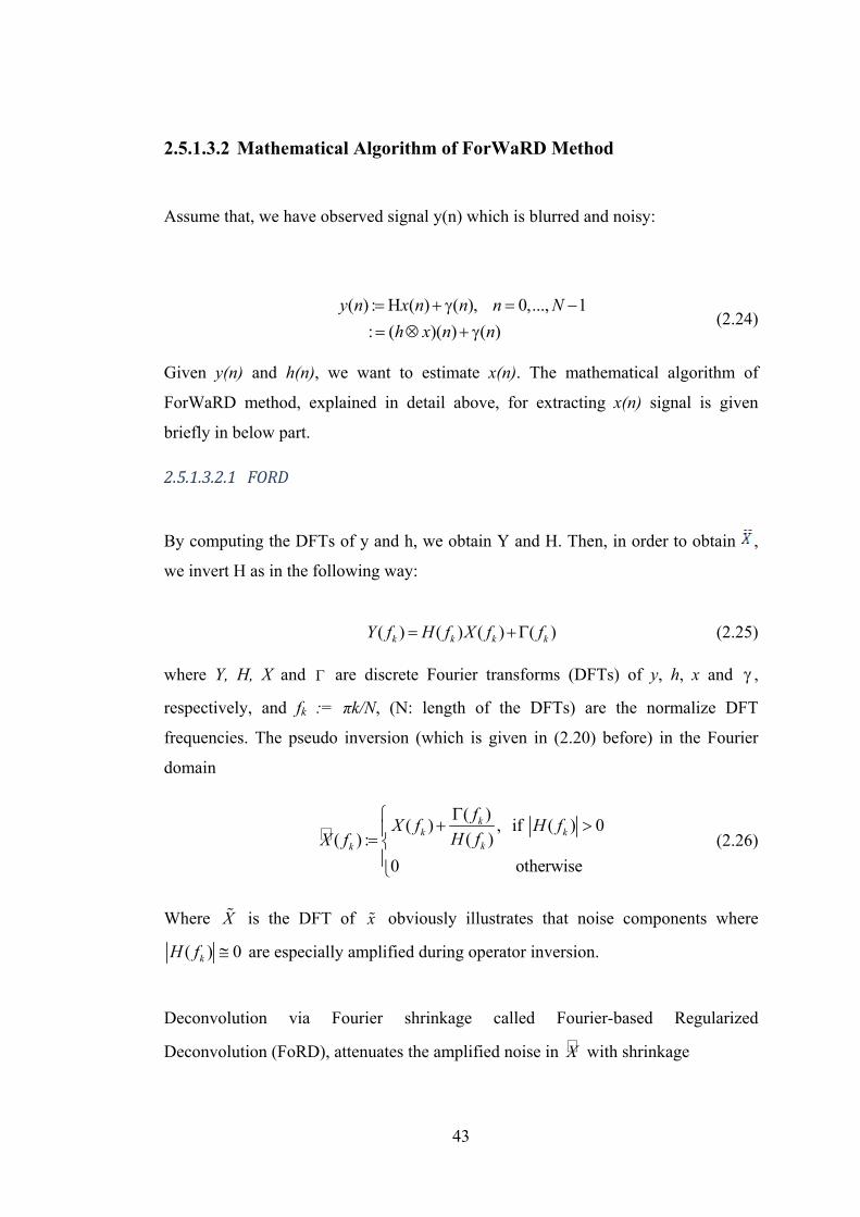
43

2.5.1.3.2 Mathematical Algorithm of ForWaRD Method

Assume that, we have observed signal y(n) which is blurred and noisy:


( ) : ( ) ( ), 0,..., 1

: ( )( ) ( )y n x n n n N

h x n n= Η + γ = −= ⊗ + γ

(2.24)

Given y(n) and h(n), we want to estimate x(n). The mathematical algorithm of

ForWaRD method, explained in detail above, for extracting x(n) signal is given

briefly in below part.

2.5.1.3.2.1 FORD

By computing the DFTs of y and h, we obtain Y and H. Then, in order to obtain ,

we invert H as in the following way:


( ) ( ) ( ) ( )k k k kY f H f X f f= + Γ (2.25)

where Y, H, X and Γ are discrete Fourier transforms (DFTs) of y, h, x and γ ,

respectively, and fk := πk/N, (N: length of the DFTs) are the normalize DFT

frequencies. The pseudo inversion (which is given in (2.20) before) in the Fourier

domainEquation Section (Next)

( )( ) , if ( ) 0( )( ) :

0 otherwise

kk k

kk

fX f H fH fX fΓ⎧ + >⎪= ⎨

⎪⎩

(2.26)

Where X% is the DFT of x% obviously illustrates that noise components where

( ) 0kH f ≅ are especially amplified during operator inversion.

Deconvolution via Fourier shrinkage called Fourier-based Regularized

Deconvolution (FoRD), attenuates the amplified noise in X with shrinkage

44


2

2

( )( ) ( )

kfk

k k

H fH f f

λ =+ Λ

(2.27)

The ( ) 0kfΛ ≥ , usually defined as regularization terms [4, 21] which control the

amount of shrinkage. The discrete Fourier transform components of the FoRD

estimate fXλ are:


( ) : ( )f fk k kX f X fλ λ= (2.28)

Using the equation (2.27) we obtain


( )

( ) : ( )( )

ff

fk

k kk

fX f X f

H fλ

λ λ

Γ= + (2.29)

The fXλ

and /f Hλ

Γ comprising fX λ denote the respective DFTs of the retained

signal fXλ

and leaked noise 1fλ

γ−Η components that constitute the FoRD estimate

% fxλ .(See equation (2.22)

Limitations of FoRD : For signals with singularities, it is not provided economical

representations in the Fourier domain, such as images with edges, due to the fact that

the energy of the singularities spreads over many Fourier coefficients.

2.5.1.3.2.2 Wavelet ShrinkageBased Signal Estimation

Economical signal representation of the wavelet transform facilitates an effective

solution to the problem of extracting the desired signal x(n) from AWGN-corrupted

observations,

45


%( ) ( ) ( )x n x n n= + γ (2.30)

Simple shrinkage in the wavelet domain with scalars λw can provide excellent

estimates of x. this shrinkage is illustrated by (2.22) with wavelet basis functions as

the bk’s.

Oracle thresholding [75] shrinks with


,,

,

1, if | |>

0, if | |j l jw

j lj l j

w

w

σλ

σ⎧ ⎫⎪ ⎪= ⎨ ⎬≤⎪ ⎪⎩ ⎭

(2.31)

where 2jσ is the noise variance at wavelet scale. It is provided an excellent

estimation by oracle thresholding. However, it is impractical because of the

assumption of knowledge of the wavelet coefficients ,j lw of the desired x. Hard

thresholding, which has similar performance to the Oracle thresholding and it is also

practical. Hard thresholding employs,


~

,

, ~

,

1, if | |>

0, if | |

j l j jwj l

j l j j

w

w

ρ σλ

ρ σ

⎧ ⎫⎪ ⎪= ⎨ ⎬⎪ ⎪≤⎩ ⎭

(2.32)

where ~ ~

, ,: ,j l j lw x ψ=< > , and jρ is a scale-dependent threshold factor.

In practice, the Wavelet-domain Wiener Filter (WWF) improves on the MSE

performance of hard thresholding by employing Wiener estimation on each wavelet

coefficient.

46

WWF chooses


2

,, 2 2

,

| || |

j lwj l

j l j

ww

λσ

=+

(2.33)

We have % fxλ signal after processing the FORD algorithm. In this step compute

Discrete Wavelet Transform of the still noisy % fxλ to obtain wavelet coefficients

, ; fj lw

λ

( . Shrink, ; fj l

wλ

( with ,wj lλ using (2.33) (shrinkage (thresholding) parameters in

wavelet domain) to obtain new thresholded wavelet coefficients: , ,, ;ˆ : f

wj l j lj l

w wλ

λ= ( .

Compute the inverse DWT with the ,ˆ j lw to obtain the ForWaRD estimate x .

2.5.2 Clustering of Hemodynamic responses as active and passive

The main objective of our thesis is to identify brain activation from fMRI signals. In

order to identify active regions in brain according to the incoming stimulant, we

should determine which brain voxels are active, which ones are passive. This

information is included in voxels’ hemodynamic response functions’ shapes, as

explained briefly in previous section. Once the necessary hemodynamic response

functions’ shapes are extracted, we need to cluster these to determine active versus

passive groups.

We mentioned that hemodynamic response’s shape determines the activity and

passivity of the underlying voxel. If it is active the intensity of the hemodynamic

response function has a peak like left picture in the Figure1.2. The values of this

peak, as well as its latency change in a large definite interval. This situation causes

ambiguity when clustering hemodynamic responses. So, we need a clustering method

which should work in ambiguous situations. The best method for these situations is

fuzzy C means clustering in literature, so we decided to use this clustering method

for our problem. The basis of this algorithm is explained in below.

47

In fuzzy clustering, each point has a degree of belonging to clusters, as in fuzzy

logic, rather than belonging completely to just one cluster. Thus, points on the edge

of a cluster, may belong to the cluster with a lesser degree than points in the center of

cluster. For each point x we have a coefficient giving the degree of being in the kth

cluster uk(x). Usually, the sum of those coefficients for any given x is defined to be 1:


.

1

( ) 1num clusters

kk

x u x=

⎛ ⎞∀ =⎜ ⎟⎝ ⎠

∑ (2.34)

With fuzzy k-means, the centroid of a cluster is the mean of all points, weighted by

their degree of belonging to the cluster:


( )( )

mkx

k mkx

u x xcenter

u x= ∑

∑ (2.35)

The degree of belonging is related to the inverse of the distance to the cluster center:


1( )

( , )kk

u xd center x

= (2.36)

then the coefficients are normalized and fuzzyfied with a real parameter m>1 so that

their sum is 1. So Equation Section (Next)

2/( 1)1( )

( , )( , )

k m

kj

j

u xd center xd center x

−=⎛ ⎞⎜ ⎟⎜ ⎟⎝ ⎠

∑ (2.37)

For m equal to 2, this is equivalent to normalizing the coefficient linearly to make

their sum 1. When m is close to 1, then cluster center closest to the point is given

much more weight than the others, and the algorithm is similar to k-means.

48

The fuzzy c-means algorithm is very similar to the k-means algorithm:

• Choose a number of clusters.

• Assign randomly to each point coefficients for being in the clusters.

• Repeat until the algorithm has converged (that is, the coefficients' change

between two iterations is no more than ε , the given sensitivity threshold):

o Compute the centroid for each cluster, using the formula above.

For each point, compute its coefficients of belonging to the clusters, using the

formula above.

49

CHAPTER 3

METHOD

3 METHOD

In our thesis, basic aim is to identify voxel based activation of the brain based on

processing fMRI signals. We have to perform two sub goals in order to realize our

main aim. Firstly, we have to extract the hemodynamic response function from fMRI

signal whose shape is information about voxels situation as active or passive by

using a deconvolution algorithm. We adapt the direct Fourier Wavelet Regularized

Deconvolution (ForWaRD) method to our fMRI problem in order to extract

hemodynamic response from fMRI signal. In Chapter 2, we layed the necessary

mathematical background related to ForWaRD. In this chapter we express how we

adapted direct ForWaRD to our fMRI problem. Secondly, hemodynamic responses

of voxels have to be clustered in order to decide which HRF resulted from active

voxels and which ones from passive voxels. Our clustering method is fuzzy c-means

algorithm with laplacian eigenmaps. In previous chapters we mentioned the

generalities about this method, now we depict how we use it ın our problem.

The block diagram of our system for fMRI problem is given below, details are in the

following parts.

Figure3.1 System Diagram of the Thesis

50

3.1 How ForWaRD is Adapted for Hemodynamic Response Function Extraction

The extraction of hemodynamic response function (HRF) from FMRI data is the

focus of this subsection. Fourier-wavelet regularized deconvolution (ForWaRD]

which was developed recently [76] is adapted for use in our FMRI problem. The

important point is that this method is directly implemented for the first time to fMRI

signals, we do not change its mathematical formulation. In fact, this method was

developed for denoising and deblurring images [76]. ForWaRD combines frequency

domain deconvolution with frequency domain regularization and wavelet domain

regularization. Each of these phases will be introduced and demonstrated on fMRI

signals in the coming subsections of this chapter. The advantage of deconvolution in

the frequency domain is identifying overlapping signals. Its main disadvantage is

noise amplification. Noise can be reduced in the frequency domain by shrinking

frequency coefficients but it is may be difficult to separate noise and signal.

ForWaRD solves this problem by using wavelet domain shrinkage [20]

Our adaptation of the ForWaRD method uses an FMRI data set and the stimulus time

pattern. Mathematically, FMRI signal can be modeled as;

Equation Chapter (Next) Section 1

( ) ( * )( ) ( )g n h f n e n= + (3.1)

g(n): FMRI signal, h(n): hemodynamic response function, f(n): stimulus pattern, e(n):

noise. ForWaRD uses known fMRI signal g(n) and stimulus pattern f(n) to estimate

unknown hemodynamic response h(n).

When this method is compared with the other HRF extraction methods, reviewed in

Chapter 2, it has some important advantages. It takes overlapping responses into

account and is much simpler than reviewed methods in Chapter 2, due to the fact that

it does not rely on shape assumptions of the HRF: using only the FMRI signal and

the stimuli, we determine the extracted time points: so, this method is data driven

instead of model driven. This property means that HRF is not biased by any a priori

51

model.

The outline of the extraction of HRF from FMRI data part of the Chapter 3 is

organized as follows. Section 3.1.1 mentions the general linear model which is used

in ForWaRD extraction algorithm. Section 3.1.2, Section 3.2 and its subsections

explain the extraction algorithm of ForWaRD for fMRI signals.

3.1.1 Determining the HRF

fMRI signals are responses obtained by patients processing stimula. Therefore, those

stimula are inputs to the patient brain as activation are processed there, leading to

measured fMRI signals.

The process is formulated by the measured signal g representing a single response to

a pattern f of stimuli being a convolution of stimulus pattern f with the brain activity

impulse response h, plus an additive term representing noise.


( ) ( * )( ) ( ), 1,....,g n h f n e n n N= + = (3.2)

g(n): FMRI signal

h(n): hemodynamic response function

f(n): stimulus pattern

e(n): noise

with ‘*’ denoting discrete convolution. (reviewed in Section 1.1.1 in Chapter 1).

The brain activity responding to a stimulus is represented as a hemodynamic

response function as defined by h(n) above.

52

A convolution in the time domain is defined as a pointwise multiplication in the

frequency domain, and a deconvolution is a pointwise division:


( ) ( ) ( ) ( ), k 1,....,G k H k F k E k N= + = (3.3)

where F(k), G(k) and H(k) denote the Fourier transforms of f(n), g(n) and h(n),

respectively. In the absence of noise e(n) and if f and g are given, the Fourier

Transform of hemodynamic response is computed by pointwise division as follows:


( )( )( )

G kH kF k

= (3.4)

In the presence of noise, the Fourier Transform of the estimation of the

hemodynamic response function, called hest, is obtained by pointwise division:


( ) ( )( )( ) ( )

G k E kH kF k F k

= + (3.5)

Where ( )( )

G kF k

is the estimate of H(k), called Hest(k). Then the equation becomes as

follows:


( )( ) , if | ( ) | 0( )( )

0 otherwise

E kH k F kF kHest k

⎧ ⎫+ >⎪ ⎪= ⎨ ⎬⎪ ⎪⎩ ⎭

(3.6)

Noise is amplified at frequencies k where F(k) is small,. If F(k) =0, the deconvolution

problem becomes singular and such systems are called ill-conditioned.

Deconvolution of noisy signals which are output of the ill-conditioned systems is an

ill posed-problem. Our FMRI problem is an ill-posed problem because F(k), stimulus

pattern, can be zero at some frequencies (see Figure3. 2).

53

Figure3. 2 Example of a block design stimulus pattern and its Fourier transform

It may not be possible to obtain a unique solution or solution can be meaningless or

at best unstable: when a noise is amplified at frequencies k, where F(k) is close to

zero, parts of the noise e may appear in the extracted response. The regularization

methods in the frequency and wavelet domains are used in ForWaRD algorithm to

cope with this problem. The ForWaRD regularisation scheme, used in the thesis, is

described in Section 3.2, the general block diagram of the ForWaRD as will be

treated in the thesis is given in Figure3.3:

Figure3.3 Block Diagram of ForWaRD

54

3.1.2 Regularization

3.1.2.1 Shrinkage I: the Frequency Domain

For one stimulus, one response function and additive noise, our fMRI deconvolution

becomes as in the equation (3.2). An estimate Hest of the Fourier transform of hest is

shown in (3.6) in the previous part.

Deconvolution via Fourier shrinkage attenuates the amplified noise in the Fourier

transform estimate of HRF as Hest(k) after the pointwise division with wiener

shrinkage, by multiplying each frequency coefficient Hest(k) by a wiener shrinkage

factor fkλ :


2

2~

22

| ( ) |( )

| ( ) || ( ) |

fk

e

F kkNF k

H k

λστ

=

+

(3.7)

τ : regularization parameter

eσ :the variance of the noise e(n)

N :length of data

For our thesis, the estimation of the noise level eσ from the data is important rather

than to assume that the noise level is known. We compute an estimate from the finest

scale empirical wavelet coefficients: ( )| |e nMedian wσ = where wn is the finest

wavelet coefficient vector at level n and n is the maximum decomposition level

corresponding to these wavelet coefficients. We believe it is important to use the

median estimator, in case the fine scale wavelet coefficients include a small ratio of

strong “signals” mixed in with “noise”.

55

Another important point here is to identify the wiener shrinkage factor λ (k). We

desire to choose the shrinkage factor that minimizes the ForWaRD MSE:2

, 2ˆh hλ κ−

h : original hemodynamic response

,hλ κ : ForWaRD estimate hemodynamic response

However, since the original HRF is unknown, we define an observation based cost

and choose shrinkage factor that minimizes this cost.

Observation based cost function:

F(fk) : Fourier transform of stimulus pattern

,ˆ ( )kH fλ κ : Fourier transform of ForWaRD estimate hemodynamic response

In the observation based cost function the stimulus pattern F(fk) and fMRI signal

G(fk) is known so they can not be changed during the computations of desired

hemodynamic response function. Therefore, only the regularization parameter τ

changes the extracted hemodynamic response function in the underlying observation

based cost. Because regularization parameter is important we define it as a

probability vector based variable. In order to obtain minimum value for the

observation based cost, we change regularization parameter in a vector and find the

optimum value.

We compute regularization parameter τ as: 2 222 2

[0, 01 0, 05 0,1 0,5 1 5 10] / ( )N f y yτ σ μ= × −

Vector A

Values of vector A change according to the problem We calculate each τ based on

each element of determined vector A. For each calculated τ value, we calculate the

observation based cost function value. Calculated cost values are saved to a vector

respectively. The smallest cost value is chosen from this vector and the τ value

which was used in order to calculate this cost is determined. This τ value is our

optimum regularization parameter. Shrinkage factor is calculated based on this value.

After computing shrinkage factor we shrink Hest(k) with this λ(k) (see equ 3.9). In

this way we suppressed the amplified noise components in this step.

2/2 2

,2( /2) 1

( ) 1 ˆ( ) ( ) ( )( )( )

Nk

k k kk N kk

F fF f H f G f

F fF fλ κ

τ=− +

−+

∑

56

The discrete Fourier transform (DFT) components of the deconvolution via Fourier

shrinkage estimate hλ are:


( ) : ( ) ( )fest kH k H k kλ λ= (3.8)


2 2

2 2~ ~

2 22 2

| ( ) | ( ) | ( ) |( ) : ( )( )

| ( ) | | ( ) || ( ) | | ( ) |

e e

F k E k F kH k H kF kN NF k F k

H k H k

λ

σ στ τ

⎛ ⎞ ⎛ ⎞⎜ ⎟ ⎜ ⎟⎜ ⎟ ⎜ ⎟

= +⎜ ⎟ ⎜ ⎟⎜ ⎟ ⎜ ⎟

+ +⎜ ⎟ ⎜ ⎟⎝ ⎠ ⎝ ⎠

(3.9)


( )( ) : ( )( )

E kH k H kF k

λλ λ= + (3.10)

The ( )H kλ and ( )( )

E kF k

λ comprising ( )H kλ denote the respective Discrete Fourier

Transforms of the retained signal hλ and leaked noise 1F eλ− components that

comprise the deconvolution via fourier domain wiener shrinkage estimate hλ .

Briefly, when an estimate eσ (the noise variance e(n)) and a regularization factor τ is

given, each frequency coefficient of Hest(k) is multiplied with a fkλ for attenuating

the noise and the result is ( )H kλ .

The hemodynamic response function estimate hλ (n) is the inverse Fourier transform

of ( )H kλ . Wiener shrinkage minimizes 2

h hλ − . Where F(k) is large, ( )k 1fkλ ≈ and

where F(k) is small, ( )k 0fkλ ≈ . In order to remove noise from smooth signals

wiener shrinkage is the optimal method, but signals which have irregularities (such

as steep edges) are handled less well. “Irregularities contain high frequencies, so

either noise is not suppressed, or artifacts (such as ringing) occur.” [76].

57

Optimal values for the regularization parameter τ in above equations are obtained

from the strength of the signal and of the noise.

3.1.2.2 Shrinkage II: Wavelets and ForWaRD

After Fourier domain inversion step we obtain noisy deconvolution Hest(k) of desired

hemodynamic response signal h(n). Because of the unsatisfactory result of Fourier

inversion, we use Fourier domain regularization with wiener shrinkage. This

frequency domain shrinkage attenuates the noise by multiplying each frequency

coefficient of Hest(k) by fkλ (k) and through this shrinkage we obtain regularized

deconvolution ( )H kλ . Since ( )H kλ is still noisy, ForWaRD implements another

regularization to deconvolved signal ( )H kλ in wavelet domain, to filter the rest of

the noise. In this part of the Chapter 3, we will mention wavelet domain

regularization in detail.

Briefly, as we mentioned “ForWaRD regularizes the deconvolution with both

frequency domain and wavelet domain shrinkage” [82]. ForWaRD uses wavelet

domain wiener shrinkage because Fourier domain shrinkage does not adequate to

filter the whole noise in fMRI signal. Wavelet domain Wiener (and also Tikhonov)

shrinkage is a very muscular regularization method for signals with irregularities. It

needs an estimate of the regular part of the signal. Wavelet transform is used in the

ForWaRD method to obtain this estimate.

A discrete wavelet transform defines a sampled signal c0 of length N as a sum of

localised basis functions. We write the regular part c1 and irregular part d1 as

weighted sums of shifted and dilated versions of a scaling function and wavelet

function ψ, respectively. By dividing subsequent cj into cj+1 and dj+1 analysis at

multiple levels is done. The underlying inverse wavelet transform uses cj and dj to

reconstruct cj−1.

In general, a DWT with J levels of decomposition JϵN recursively separates the

signal into a regular part cJ and detail signals d1,d2…dJ

58

Wavelet domain Wiener shrinkage is applied to the estimate hλ by ForWaRD. For

smooth signals, most energy is stored in the approximation part cJ, and the

coefficients of dj are small [80]. In the underlying signal, large coefficients of dj

appear at irregularities. The regular and irregular parts of the signal are separated: cJ

and large coefficients of dj are regarded as signal, the rest is noise. Wavelet Domain

Wiener Filtering is executed via two wavelet transforms. Two different wavelet

transforms of hλ , represented by the basis functions ( 1,ψ1) and ( 2,ψ2),

respectively, are similar. ForWaRD uses first estimate of is obtained by computing

the Discrete Wavelet Transform of hλ , using ( 1,ψ1), and thresholding the detail

coefficients { }1 1( ) ( 1, ........., / 2 )

Jj j

jd n n N

== to remove noise. After thresholding,

result is thresholded detail coefficients 1 ( )j

d n−

.

This estimate of the wavelet spectrum of the desired signal is used in the wavelet

domain Wiener shrinkage (second step). After computing a second Discrete Wavelet

Transform using ( 2,ψ2), its detail coefficients are shrunk [6]:


,2 2

2

1

2~

1

( ) ( ) ( ), where

( )( )

( )

j j j

j

jj

e

d n d n n

d nn

d n

κ κ

κσ

−

−

=

=+

(3.11)

We estimate the noise standard deviation eσ using the median absolute value (MAD)

of the first-level detail coefficients [80].

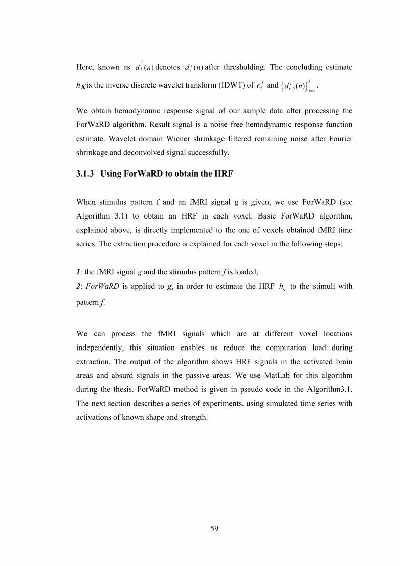
59

Here, known as 1 ( )j

d n−

denotes 1 ( )jd n after thresholding. The concluding estimate

hκ is the inverse discrete wavelet transform (IDWT) of 2jc and { },2 1

( )Jj

jd nκ =

.

We obtain hemodynamic response signal of our sample data after processing the

ForWaRD algorithm. Result signal is a noise free hemodynamic response function

estimate. Wavelet domain Wiener shrinkage filtered remaining noise after Fourier

shrinkage and deconvolved signal successfully.

3.1.3 Using ForWaRD to obtain the HRF

When stimulus pattern f and an fMRI signal g is given, we use ForWaRD (see

Algorithm 3.1) to obtain an HRF in each voxel. Basic ForWaRD algorithm,

explained above, is directly implemented to the one of voxels obtained fMRI time

series. The extraction procedure is explained for each voxel in the following steps:

1: the fMRI signal g and the stimulus pattern f is loaded;

2: ForWaRD is applied to g, in order to estimate the HRF hκ to the stimuli with

pattern f.

We can process the fMRI signals which are at different voxel locations

independently, this situation enables us reduce the computation load during

extraction. The output of the algorithm shows HRF signals in the activated brain

areas and absurd signals in the passive areas. We use MatLab for this algorithm

during the thesis. ForWaRD method is given in pseudo code in the Algorithm3.1.

The next section describes a series of experiments, using simulated time series with

activations of known shape and strength.

60

Algorithm3.1 ForWaRD in pseudo-code

61

Illustration of ForWaRD algorithm with a sample data step by step:

Step1:Fourier Inversion

Figure3.2, shows the flow of the process within the ForWaRD algoritm.. Now we

will give an example with a simulated fMRI data that will show the flow of the

algorithm step by step and the results of the algorithm after each step. Thus, we will

able to understand how ForWaRD extracts hemodynamic response function from an

fMRI signal.

First, we have the observation signal g, called FMRI data in the beginning of the

algorithm. One sample of FMRI data is given in Figure3.4

0 20 40 60 80 100 120 140-100

-50

0

50

100

150Observed fMRI Signal

Time Point

Figure3.4 fMRI signal.

62

ForWaRD first performs fourier inversion step. In this step observed fMRI signal is

deconvolved in order to obtain hemodynamic response. The result of this step is

given in Figure3.5.

0 20 40 60 80 100 120 140-80

-60

-40

-20

0

20

40

60

80

100After Fourier Inversion (without Regularisation)

Time Point

Figure3.5 Output of Fourier inversion step

After Fourier inversion because of the structure of fMRI signal stimulus pattern, we

cannot obtain a satisfactory estimate. Since, the stimulus is much closer to zero in

some places, the noise is extremely amplified. As we mentioned before, when a noise

is amplified at frequencies k, where stimulus pattern is close to zero, parts of the

noise may appear in the extracted response. So, we need some regularization in order

to attenuate noise components. We know from previous parts, ForWaRD uses the

regularization methods in the frequency and wavelet domains. Frequency

regularization is performed first.

63

Step2:Fourier Shrinkage

0 20 40 60 80 100 120 140-8

-6

-4

-2

0

2

4

6

8

10Deconvolved Noisy HRF

Figure3.6 Deconvolved HRF After Fourier Shrinkage

After fourier shrinkage step noise component are attenuated. But result deconvolved

HRF is still noisy. In order to filter remaining noise on deconvolved HRF signal,

ForWaRD performs wavelet domain regularization.

64

Step3:Wavelet Shrinkage

0 20 40 60 80 100 120 140-1

0

1

2

3

4

5

6

7

8Deconvolved and Denoised HRF

Time Points

Figure3.7 ForWaRD - Extract deconvolved and denoised HRF from fMRI signal

After the last step called wavelet regularization, we have achieved very satisfactory

result as a result of the program. HRF shape is similar to the ideal one which is

explained in Chapter 1.

Thus we have proven the program is working correctly and it is very robust to the

noise on fMRI signal. Detailed experiments and results related with the performance

and correct operation of the program are given in the next section.

65

3.2 Clustering

3.2.1 Clustering of FMRI data

At the start of the thesis work, we have a blurred and noisy FMRI signal and our aim

is to find which voxels in the brain are active which ones are passive. We mentioned

that FMRI signals include hemodynamic response signals that possess in their shape,

information about whether a voxel is active or passive. In order to achieve

information about voxel activity and passivity, we have to extract hemodynamic

response from FMRI signal. The way of extracting hemodynamic response from

FMRI signal is to apply deconvolution process on FMRI.

Therefore, in the first part of the thesis, a wavelet based deconvolution method called

ForWaRD is applied to the FMRI and obtained hemodynamic responses from FMRI

signal. Every voxel has a unique hemodynamic response.

In this part of the thesis, we want to classify the estimated HRF patterns as generated

from active and passive voxels by use of a clustering algorithm. Separation can be

done through the pattern information in hemodynamic responses. Analyzing possible

relations between different active voxels’ hemodynamic responses and in the same

way, analyzing possible relations between different passive voxels’ hemodynamic

responses is the start point of the clustering because active voxels posess similarities

in HRF and likewise, passive voxels have separate similarities in HRF. By defining a

similarity measure between different hemodynamic response signal time series, we

aim to group voxels with similar properties. If we group hemodynamic response

signals according to their similarities meaning voxels with similar properties, active

and passive signals will be separated from each other.

3.2.2 Clustering Algorithm Outline

The investigated algorithms are explained in Chapter 2. After investigations of

methods and some sample tests, we decided to use fuzzy c means algorithm with

nonlinear dimension reduction of hemodynamic responses. The reason for providing

66

Using the fuzzy c means approach can be explained as follows: We mentioned that

hemodynamic response’s shape determines the activity and passivity of the voxel. If

it is active the waveform of the hemodynamic response function has a peak like in

the left picture of Figure1.2. The values of this peak are not definite numbers, they

are changing in a large definite interval. This situation causes ambiguious when

clustering hemodynamic responses. So, we need a clustering method which should

work in ambiguity situations. The best method for these situations is fuzzy C means

clustering, so we decided to use this clustering method for our fMRI problem. Even

though these features are advantageus for our classification problem, fuzzy c means

has some limitations. Because, fMRI time series have poor signal to noise ratio

(SNR) and confounding effects -mean kinds of noises-, sometimes we obtain

unsatisfactory clustering results on the time series. As a result data are not

necessarily grouped according to the similarity of their pattern of response to the

stimulation. Moreover, increasing the dimension of the clustering space leads to

practical difficulties such as “curse of dimensionality.” Besides its advantages,

because of these poor features of fuzzy c means, we combine this method with

Laplacian Embedding. This method includes dimension reduction of activation data.

For nonlinear dimension reduction, there are several methods in literature such as

Locally Linear Embeddings (LLE)[5], Isomap [6], and Laplacian Embeddings [2].

We decided to use the Laplacian method. The power of this Laplacian Embedding

method is to detect significant structures within the noisy and complex dynamics of

hemodynamic response signals. This Laplacian Embedding Approach with fuzzy c-

means clustering is called Laplacian Eigenmaps Method. [1]

67

3.2.2.1 Laplacian Eigenmaps Algorithm

Suppose that our FMRI data set is converted to N x T matrix. Let N be the voxel

order and T be the time point. Each row shows the time series which is obtained for

one voxel.

For each voxel (with 1...T time points):

• Step 1: Obtain adjacency graph using n-nearest neighbors where the Cosine

similarity is used. So for each voxel we obtain the similarities with respect to

other voxels.

• Step 2: After calculation of similarities, weights are calculated using Distance

method where binary similarity measure is assigned as weight wij.

• Step 3: Evaluate eigenvectors using generalized eigenvector problem. These

eigenvectors will be used in Fuzzy C-Means algorithm.

• Step 4: After calculation of eigencvectors, we choose some of them to use in

Fuzzy C-Means algorithm. Then we set the cluster number as three which are

active, passive and motion.

It is briefly mentioned above which steps are followed while clustering

hemodynamic response function signals -obtained from fMRI signals- with

Laplacian eigenmaps algorithm. Now, each step will be explained in detail and the

application of Laplacian eigenmaps method to fMRI will become more clear.

STEP 1 - Adjacency Graph Construction

Given k points x1, x2, x3, ….., xk in l , we put an edge between nodes i and j if xi and

xj are “neighbour”. There are two variations:

1. ε- neighborhoods where ε ∈ . Nodes i and j are connected by an edge if 2

– i jx x ε< where the norm is Euclidean Norm in l .

68

2. n-nearest neighbors where n N∈ . Nodes i and j are connected by an edge if i is

among n nearest neighbors of j or j is among n nearest neighbors of i. N-nearest

neighbors can be calculated using two metrics which are Euclidean distance and

Cosine similarity.

i. Euclidean Distance: In cartesian coordinates; p = (p1, p2, .., pn) and q = (q1, q2,

.., qn). Euclidean distance from p to q:


2 2 2 21 1 2 2

1( , ) ( , ) ( ) ( ) ......( ) ( )

n

n n i ii

d p q d q p q p q p q p q p=

= = − + − + − = −∑ (3.12)

ii. Cosine Similarity: It is a similarity measure which can be obtained by

evaluating the cosine between two vectors. If the angle is 0, the cosine is equal to

1, for other cases it is smaller than 1. So if we calculate the cosine of the angle

between two vectors, it shows us how these vectors are similar directions. Cosine

similarity:


1

2 2

1 1

.cos( )( ) ( )

n

i ii

n n

i ii i

A xBA Bsimilarity

A BA x B

θ =

= =

= = =∑

∑ ∑ (3.13)

69

STEP 2 – Choosing Weight

There are three variations for weighting the edges:

1. Heat Kernel: [ ]t ∈ . If nodes i and j are connected, put


2

i jx x

tijw e

−−

= (3.14)

2. Distance: If nodes i and j are connected, Euclidean distance or

Cosine similarity are assigned as weight wij

3. Simple-Minded: If nodes i and j are connected, wij = 1.

STEP 3 – Eigenmaps

Eigenvalues and eigenvectors computation with respect to generalized eigenvector

problem:


Lf Dfλ= (3.15)

where

D: diagonal weight matrix

Diagonal weight matrices entries are row (or column since W is symmetric) sum of

W,


ii ji

jD W

L W D

=

= −

∑ (3.16)

where L is Laplacian matrix .

Let f0, f1, …, fk-1 be solutions of equation (3.15), ordered according to their

eigenvalues,

70


0 0 0

1 1 1

2 2 2

3 3 3

1 1 1

0 1 2 1

...

0 .....

k k k

k

Lf DfLf DfLf DfLf Df

Lf Df

λλλλ

λ

λ λ λ λ

− − −

−

====

=

= ≤ ≤ ≤

(3.17)

We leave out the eigenvector f0 corresponding to eigenvalue 0 and use the next m

eigenvectors for embedding in m-dimensional Euclidean space where m<k.


1( ( ),......., ( ))i mx f i f i→ (3.18)

STEP 4 – (Clustering): Fuzzy C-Means (FCM)

In fuzzy clustering, each point has a degree of belonging to clusters, as in fuzzy

logic, rather than belonging completely to just one cluster. Thus, points on the edge

of a cluster, may be in the cluster to a lesser degree than points in the center of

cluster.

Fuzzy C-Means algorithm minimizes the cost function below.


2

1 1, 1

N Cm

m ij i ji j

J u x c m= =

= − ≤ ≤ ∞∑∑ (3.19)

Algorithm is started by assigning a random value for membership matrix. And for

the second step center vectors are calculated with the equation below.

71


1

1

Nm

ij ii

j Nm

iji

u xc

u

=

=

=∑

∑ (3.20)

Finally the matrix U is calculated again using the equation below. Then the new U

matrix is compared with the old one. The process continues until the difference

between U matrices become smaller than ε.


2( 1)

1

1ij

mCi i

k i k

ux cx c

−

=

=⎛ ⎞−⎜ ⎟

−⎝ ⎠∑

(3.21)

After the clustering processing, U membership matrix which contains fuzzy values

gives the result of clustering.

72

CHAPTER 4

EXPERIMENT RESULTS AND DISCUSSIONS

4 EXPERIMENT RESULTS AND DISCUSSIONS

4.1 Experimental Design Types

Within the literature, there are two basic types of fMRI studies: Block designs and

event-related designs.

4.1.1 Block design paradigm

A blocked design presents two or more conditions in an alternating pattern.

Experimental conditions are separated into distinct blocks, so that each condition is

presented for an extended period of time. Most early fMRI studies used blocked

designs. For example in [41], a bright visual pattern was presented for 60s and then

the display was dark for 60s. This approach can be classified as an “ABABAB…”

blocked design. In most fMRI studies, each block is about 10 to 30s in duration, and

there may be many alternations between different block types in a single run.

Example of a block design paradigm is given below:

0 20 40 60 80 100 120 140 160 1800

0.5

1

1.5

Figure4.1 Example of a block design stimulus pattern

73

4.1.2 Event-related design paradigm

Event-related design is the presentation of discrete, short duration events whose

timing and order may be randomized. In an event-related design, stimuli are

presented as individual events, or trials. The study by Blamire and colleagues in 1992

[83] was the first to present event-related data. In slow event-related designs, the

hemodynamic response decays to baseline after each stimulus, which allows the

response to each trial to be individuated. In rapid experiments, the events are

presented sufficiently close together (i.e., less than 10s) so that the hemodynamic

response does not have time to decay to baseline between successive stimuli. For fast

designs, special analysis procedures are required to separate the hemodynamic

responses to different events. Example of a event- related design paradigm is given

below:

0 5 10 15 20 25 30 35 40 45 50-0.5

0

0.5

1

1.5

Time Point

Event Related Stimulus Pattern

Figure4.2 Example of a event-related design stimulus pattern

In this thesis, we aim at understanding the activation areas of brain by means of

determine active and passive voxels in the brain during a specific experiment. Two

sub algorithms are performed sequentially using the simulated and real data which

are comparatively analyzed after individual results analyses. First algorithm, called

ForWaRD, is performed to extract HRF information performing to voxel’s activity or

passivity included in FMRI signal as reviewed in Chapter 1 and the second sub

algorithm, called Laplacian Eigenmaps, is performed to separate active and passive

voxels by classifying hemodynamic response functions obtained in first step. These

74

two different algorithms are performed for fMRI signals obtained from all

experiments in order to identify brain activation.

In this chapter initially, we created a set of simulated fMRI data based on the Balloon

Model [86, 87] and the flow-inducing signal model presented in [88]. The aim of

creating this set of simulated fMRI data is to test the performance of our proposed

method. The experiment results (extracted hemodynamic response function shapes

and clustering results of simulated fMRI data) are shown in this chapter (in the

following subparts). A detailed performance analysis will be performed in the

Chapter 5 using the results obtained in Chapter 4.

In addition to the experiment with simulated data, in this chapter we will explain two

different experimental results, performed with real block design fMRI data.

4.2 Experiment Results

Chapter 4 presents results in two subparts. These are:

1. Results of Extracted HRF with ForWaRD Algorithm

2. Clustering Results and Identification of Active and Passive Voxels in Brain

Every subpart includes results for three different experiments, obtained from three

different fMRI data. These experiments are conducted with:

1. Simulated data with BOLD response modeled based on the Balloon Model

2. Real data from a specified fingertapping experiment

3. Real data from a specified fMR adaptation paradigm.

75

4.2.1 Results of Extracted HRF with ForWaRD Algorithm

In this part, we will analyze results from three different experiments. Adapted for

fMRI data, Fourier Wavelet Regularized Deconvolution (ForWaRD) method is

executed for extraction of hemodynamic response functions (HRF’s) from fMRI

signals. For each data, obtained HRF results are analyzed and discussed in the

following subsections.

4.2.1.1 Experiment 1: HRF Results of Simulated Data Based on the Balloon Model

In this experiment, we used a set of simulated fMRI data which is generated based on

the Balloon Model [86, 87] and the flow-inducing signal model presented in [88].

The parameters for the simulation of fMRI signal are taken to be same as in [88] that

is: ε=0.5, τS= 0.8, τf= 0.4, τ0= 1, α= 0.2, E0 = 0.8, V0 =0.02 and the stimulus pattern

and simulated ideal pure (without noises) fMRI time series (BOLD response) are

shown in Figure4.3.

We include four noise sources to the basic fMRI signal.

1. Additive white gaussian noise (AWGN)

2. Sampling jitter

3. Lag

4. Drift (linear and quadratic slope; increasing or decreasing with variable

values).

The time series of the neighboring voxels of a target voxel are also generated with

the same noise parameters.

In Figure4.3, an example block design stimulus pattern of this simulated data

experiment and the response in form of a simulated ideal BOLD response are shown.

This BOLD response is a pure and ideal form of the fMRI signal (reviewed in

Chapter 1 Figure1.3 and Figure1.4) which is modeled based on Balloon Model.

76

0 50 100 150 200 2500

0.5

1

Stimulus Pattern

Ttime Points

0 50 100 150 200 25095

100

105

110BOLD Response

Ttime Points

Figure4.3 Stimulus pattern and simulated pure fMRI signal, called ideal BOLD response

In this work, our main objective is to identify voxel based activation in the brain

according to the obtained fMRI signal. Active voxels can be placed anywhere in the

brain during a specific experiment, but spatial information is disregarded in our

experiment. In this part, we focus on the extraction of HRF. We analyze the accuracy

of the extracted hemodynamic response functions (HRF) which are results of

ForWaRD algorithm.

In simulations, BOLD responses are corrupted by additive noises such as additive

white Gaussian noise (AWGN), jitter, lag and drift. For varying values of noises,

ForWaRD (HRF extraction algorithm) results are investigated. Effects of noises with

different variances on the performance of ForWaRD are analyzed. In order to

evaluate the accuracy of the results of ForWaRD algorithm, we used a MSE based

evaluation criteria. After extraction of HRF with ForWaRD, obtained HRF and the

stimulus pattern of the experiment (shown in Figure4.3) are

77

convolved. In the end, an estimated BOLD response according to the ForWaRD is

obtained. In order to understand the similarity between the estimated time series and

ideal BOLD response, the MSE is computed between these signals according to the

formulation below. The more similar the ideal BOLD and the estimated BOLD are,

the more successfully ForWaRD algorithm works.


21 2

1

1 ( )N

i ii

MSE y yN =

= −∑ (4.1)

y1 : ideal BOLD signal,

y2 :estimated BOLD signal,

i :time point,

N :total time point

In addition, the performance of ForWaRD algorithm is analyzed in terms of

sensitivity and specificity measure. After ForWaRD algorithm is performed for

simulated data, obtained HRFs are clustered. Thus, we compute the sensitivity and

specificity values for active and passive clusters.

4.2.1.1.1 Jitter, Lag, Drift and Additive Noise Values and Ranges Used in Simulations

(1) fMRI signals might have lag in time. We create a uniformly distributed lag

for the BOLD signals, i.e,

x(t) x(t- Δ) where Δ~ Uniform([0, ])

(2) fMRI signals might have drift in time. We create a quadratic random drift and

add it onto the BOLD signal, i.e,

x(t) x(t) + at2+ bt where a,b ~ Normal(0,2

2Nσ )

Δ lag in time

quadratic drift in time

78

(3) fMRI signals might have noise which is mostly due to the noisy

measurement. We create a Additive White Gaussian Noise (AWGN) to simulate

such an effect, i.e,

x(t) x(t) + n(t) where n(t) ~ Normal(0,σ2)

(4) Finally, fMRI signals might also have sampling jitter which is, like AWGN,

mostly due to the jittery measurement process.

x(t) x(t + Δ(t)) where Δ(t) ~ Normal(0,σ2)

4.2.1.1.2 Extracted HRF with ForWaRD

In this part, we corrupted ideal simulated BOLD signal (shown in Figure4.3)

exclusively with AWGN only in order to understand the effects of AWGN noise on

the performance of ForWaRD. Then, we analysed performance of ForWaRD for

varying values of all artifacts such as AWGN, jitter, drift and lag. The values of

every type of artifacts changed in a specific interval. According to all varying values

of artifacts, the success of ForWaRD algorithm in retrieving HRF is observed. It is

investigated until the program worked correctly or when it started to be wrong for

each of the artifact. Finally, the special values of AWGN, drift and lag are introduced

to the BOLD response and HRF extraction performance of ForWaRD with these

values are observed. By this observation it was found out against which error

ForWaRD method was sensitive or robust. Detailed figures and explanations can be

seen in the subparts below.

AWGN noise

sampling jitter

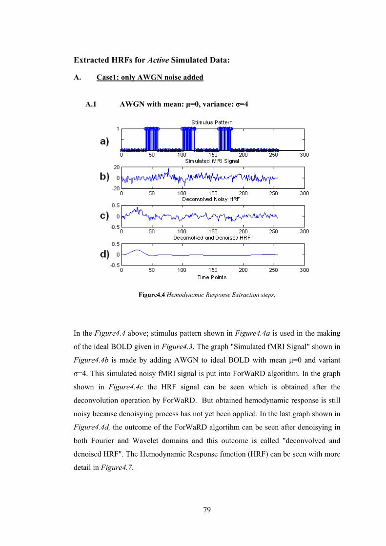
79

Extracted HRFs for Active Simulated Data:

A. Case1: only AWGN noise added

A.1 AWGN with mean: μ=0, variance: σ=4

Figure4.4 Hemodynamic Response Extraction steps.

In the Figure4.4 above; stimulus pattern shown in Figure4.4a is used in the making

of the ideal BOLD given in Figure4.3. The graph "Simulated fMRI Signal" shown in

Figure4.4b is made by adding AWGN to ideal BOLD with mean μ=0 and variant

σ=4. This simulated noisy fMRI signal is put into ForWaRD algorithm. In the graph

shown in Figure4.4c the HRF signal can be seen which is obtained after the

deconvolution operation by ForWaRD. But obtained hemodynamic response is still

noisy because denoisying process has not yet been applied. In the last graph shown in

Figure4.4d, the outcome of the ForWaRD algortihm can be seen after denoisying in

both Fourier and Wavelet domains and this outcome is called "deconvolved and

denoised HRF". The Hemodynamic Response function (HRF) can be seen with more

detail in Figure4.7.

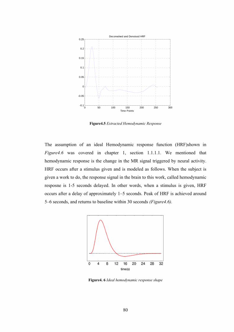
80

0 50 100 150 200 250 300-0.1

-0.05

0

0.05

0.1

0.15

0.2

0.25Deconvolved and Denoised HRF

Time Points

Figure4.5 Extracted Hemodynamic Response

The assumption of an ideal Hemodynamic response function (HRF)shown in

Figure4.6 was covered in chapter 1, section 1.1.1.1. We mentioned that

hemodynamic response is the change in the MR signal triggered by neural activity.

HRF occurs after a stimulus given and is modeled as follows. When the subject is

given a work to do, the response signal in the brain to this work, called hemodynamic

resposne is 1-5 seconds delayed. In other words, when a stimulus is given, HRF

occurs after a delay of approximately 1–5 seconds. Peak of HRF is achieved around

5–6 seconds, and returns to baseline within 30 seconds (Figure4.6).

Figure4. 6 Ideal hemodynamic response shape

81

In Figure4.7 a cumulative hemodynamic response function extracted by ForWaRD

for each train of stimuli within the On periods of the block is shown. It is shown that

the ideal assumption covered in chapter 1 is quite alike the HRF as shown in

Figure4.5. Extracted hemodynamic response shape (Figure4.7c) has a little lag in

initial part like ideal hemodynamic response and it has an acceleration which

resembles to ideal ones (Figure4.7d) when rising to the peak point and decreasing to

the baseline. In addition to that, extracted hemodynamic response has a dip after

coming to the baseline like ideal hemodynamic response. Because extracted

hemodynamic response is not as ideal as hemodynamic response shown in Figure4.6,

it diverges from base line between the 70 and 250 time points. But in spite of this, the

big part of the noise on extracted hemodynamic response is successfully filtered. As

an output of ForWaRD, a decent, almost ideal and noise-free signal is obtained.

Figure4.7 Similarity Between The Estimated BOLD and Ideal BOLD

We applied a crosscheck test in order to see if obtained HRF by ForWaRD method is

correct or not. We convolved the extracted HRF shown in Figure4.7b and the

stimulus pattern shown in Figure4.7a that is used in the experiment. This gave us an

estimated BOLD response signal as shown in Figure4.8c

82

According to the Figure4.8c and Figure4.7d, estimated BOLD signal resembles ideal

BOLD in terms of shape, the time interval where HRF’s occured and amplitude

value. But, amplitude of the estimated BOLD signal is smaller than ideal one. The

reason of that is filtering procedure of the ForWaRD algorithm. We compared

estimated fMRI and ideal fMRI signals in terms of mean square signal shown in

Table1. This evaluation parameter gives us a reliable result.



We increased the standard deviation of the noise from σ=4 to σ=8. The stimulus

pattern of this case shown in Figure4.8a is similar to previous case’s one shown in

Figure 4.7a. ForWaRD algorithm deconvolved and denoised the blurred and noisy

simulated fMRI signal shown in Figure4.8b. After processing of ForWaRD

algorithm we obtain the deconvolved and denoised hemodynamic response shown in

Figure4.8d.

83

0 50 100 150 200 250 300-0.15

-0.1

-0.05

0

0.05

0.1

0.15

0.2


Time Points


Although, we increased the standard deviation of the noise from σ=4 to σ=8, the

HRF extraction algorithm is not effected much from this increment. Though the

AWGN noise is increased, the hemodynamic response function of noisy simulated

fMRI, shown in Figure4.10 is similar with previous HRF in Figure4.7 in terms of

shape, magnitude value and activation interval, only the difference between previous

case’s HRF shown in Figure4.5 and HRF of this case shown in Figure4.9 is that,

HRF shown in Figure4.9 has initial dip between 0-4 time points intervals. The

differences can have occurred because of the characteristics of hemodynamic

response. In the literature, some studies [1] have reported an initial negative-going

dip of 1-2 seconds duration that has been attributed to a transient increase in the

density of deoxygenated hemoglobin (Chapter 1, Section 1.1.1) which is mainly

because the existing oxygen in the vessels are consumed. The simulated data is

modeled to be close to the actual real data. So, the data can normally give a result

that contains initial dip. On the other hand, increase in noise can also cause this

initial dip. When the fMRI signal is observed in Figure4.9b, it is seen that the

magnitude value of the signal's first 4 time points remains below zero because of the

noise overlaid. The ForWaRD algorithm can only smooth the noise on the signal by

deconvolution and denoising as much as seen on the Figure4.8d.

84

We applied a test in order to check whether extracted HRF by ForWaRD method is

correct or not. The extracted HRF shown in Figure4.10b and the stimulus pattern

shown in Figure4.10a are convolved. This convolution gave us an estimated BOLD

response signal as shown in Figure4.810c. The estimated BOLD response shown in

Figure4.10c resembles to the ideal BOLD shown in Figure4.10d in terms of the time

interval where HRF’s occurred, shape and amplitude value. According to these

results, ForWaRD seems to be robust against noise. But in order to understand the

performance of this method deeply we will continue to increase the noise.


When we convolved the extracted HRF in Figure4.10b and stimulus pattern in

Figure4.10a, obtained fMRI data in Figure4.10c resembles ideal one in Figure4.10d

as before but MSE gives us the most accurate similarity results. MSE results are

given in Table1.

85



We added a white Gaussian noise with standard deviation σ=10 to the ideal

simulated BOLD signal shown in Figure4.4 and obtained a very noisy simulated

fMRI signal shown in Figure4.11b. This time, after processing ForWaRD algorithm

we obtained HRF which is slightly different from ideal HRF model. Obtained HRF is

shown in Figure4.11d and Figure4.12.

86

0 50 100 150 200 250 300-0.3

-0.2

-0.1

0

0.1

0.2

0.3


Time Points


In the extracted hemodynamic response shown in Fgure4.12, the initial dip between

0-5 time points is increased according to previous results shown in Figure4.5 and

Figure4.9 because of the increased AWGN noise. The reason of this might be the

sudden signal changes due to noise or the sudden drops in the noisy "Simulated

fMRI" signal. And since the ForWaRD algorithm tries to filter the less detailed

coefficients in order to cover these sudden changes, it uses lower threshold and this

causes noise to leak into the to extracted hemodynamic response. In addition,

between time points 200 and 250, HRF signal values, which should be zero, are

corrupted and diverges from zero. Despite all this, obtained HRF with ForWaRD

preserves basic shape between 0 and 90 time points which resembles the ideal HRF

shown in Figure4.6. When we convolved the extracted hemodynamic response in

Figure4.12 with stimulus pattern, the obtained in the Figure4.13c result is satisfying

in terms of shape, magnitude values and time intervals in which HRF occurs

according to ideal BOLD response shown in Fgure4.13d.

87

Figure4.13 Similarity between The Estimated BOLD and Ideal BOLD

According to the graph above, MSE does not increase much more in the case of

increasing noise. So, ForWaRD method demonstrates to be still robust against noise.

We continue to increase noise and analyze the results.

88



When the overlayed noise is increased, or in other words, its variance becomes 12

instead of 10, there is an unwanted amount of fluctuation on the signal because of

HRF's structure. This is the 5-10 seconds long wave fluctuation which occurs when

the signal turns back to baseline after it peaks. (Figure4.41d).

0 50 100 150 200 250 300-0.25

-0.2

-0.15

-0.1

-0.05

0

0.05

0.1

0.15


Time Points


89

In Figure4.16b we can see that this fluctuation is longer than expected both in time

and amplitude. The reason of this is the raise of noise on the signal which is more

than ForWaRD can filter. This makes things difficult for ForWaRD algorithm during

deconvolution and denoising. While the ForWaRD algorithm tries to catch the real

HRF signal, because of sudden drops or rises as in intervals between 45 and 65, the

noise values might get mixed with the real HRF signal and this might cause

corruption in the output.


In Figure4.16a the stimulus pattern of the simulation experiment is shown. We can

see the extracted deconvolved and denoised hemodynamic response function signal

after executing ForWaRD algorithm in Figure4.16b, this underlying hemodynamic

response is shown detailed in Figure4.15.

The convolution of stimulus pattern in Figure4.16a and extracted hemodynamic

response in Figure4.16b is shown in Figure4.16c, called estimated fMRI signal.

When we compare estimated fMRI signal with ideal fMRI, shown in Figure4.16d,

90

we obtain the following results. Estimated fMRI and ideal fMRI signals resemble

each other in terms of structure and shape in specific time intervals and magnitude.

Magnitude value of estimated fMRI signal is lower than the ideal one. The reason of

that is the increased noise on the fMRI signal. Due to the increased noise, we loose

some of the high frequency signal components and this situation causes low

magnitude level.

A.5 AWGN with mean: μ=0, variance σ=16


We increased the noise variance from 12 to 16 in this part. We cannot distinguish

fMRI signal from the added noise shown in Figure4.17b. After increasing noise,

simulated fMRI signal becomes very noisy corrupted signal shown in Figure4.17b.

The extraction of hemodynamic response signal from this fMRI becomes very

difficult. We analyze the ForWarRD performance in this difficult situation. After

executing ForWaRD algorithm we obtain hemodynamic response function shown in

Figure4.17d. We can see the extracted HRF in Figure4.18 in a detailed manner.

91

0 50 100 150 200 250 300-0.4

-0.3

-0.2

-0.1

0

0.1

0.2


Time Points


As seen in Figure4.19, the rise in noise increases the corruption in HRF. Due to the

increased noise, ForWaRD can not extract the exact hemodynamic response signal.

We obtain corrupted hemodynamic response shown in Figure4.18.


92

In order to obtain increased noise on fMRI signal shown in Figure4.17b, we increase

noise variance from σ=12 to σ=16. While noise increases, the error between the

estimated pure fMRI in Figure4.19c obtained with the convolution of extracted HRF

with ForWaRD in Figure4.19b and stimulus in Figure4.19a, and the ideal pure fMRI

increases.

A.6. AWGN with mean: μ=0, variance σ=20


In this part, we increased the noise variance from σ=16 to σ=20, this means that the

fMRI signal shown in Figure4.20b is highly corrupted. If ForWaRD deconvolve this

simulated fMRI signal and filters noise successfully than it will be proved that

ForWaRD is very robust against noise. The result of extracted deconvolved and

denoised hemodynamic response signal is given in Figure4.20d and a detailed

explanation and detailed HRF figure is given in Figure4.21.

93

0 50 100 150 200 250 300-0.4

-0.3

-0.2

-0.1

0

0.1

0.2


Time Points

Figure4. 21 Extracted Hemodynamic Response

In Figure4. 221, even though there is a basic hemodynamic response in ForWaRD

output between time points 1 and 55, the amplitude of the negative dip between 40

and 55 is more than expected. And the noise that was not tolerated remains in the 55-

250 interval. If we were to observe how close the HRF is to the ideal signal, we

could see that the HRF is more corrupted if ForWaRD noise deviation is σ=20 and

that in wavelet domain, the real signal and noise coefficients get mixed.

But there is an important result here that needs attention. Even though the output

HRF -at the end of ForWaRD- is not so close to ideal, it still gives us information

whether the observed voxel is active or passive, because of the similarities with the

ideal signal. And the fact that this information can be obtained from such noisy fMRI

signal shows us how robust the used algorithm is against noise.

94

Figure4. 22 Similarity Between The Estimated BOLD and Ideal BOLD

The convolution process done in order to crosscheck our results can be seen in

Figure4.23. We convolved extracted HRF in Figure4.22b with stimulus pattern in

Figure4.22a and we obtain the estimated fMRI signal shown in Figure4.22c. Even

though the extracted HRF is more corrupted than previous, it still is alike the pure

fMRI signal in Figure4.22d when convolved with stimulus pattern, considering shape

and the places of peaks in time. And this proves that during analysis, the active signal

can still be separated from the passive signal.

95

A.7 AWGN with mean: μ=0, variance: σ =30


The noise variance is increased from σ=20 to σ=30. In Figure 4.23a the stimulus

pattern of the experiment is shown, in Figure4.23b the simulated fMRI signal is

shown, the deconvolved but noisy hemodynamic response function is in Figure4.23c

and the extracted hemodynamic response function with ForWaRD algorithm is

shown in Figure4.23d.

The increase in noise cannot be tolerated by the system when is increased until 30

and HRF signal is lost shown in Figure4.23d.

By the help of the analysis, it is understood that the ForWaRD method is a strong

solution for Gaussian noise changes. Even if the noise is increased above expected

levels, this method can still extract the HRF. We had to overlay an extreme amount

of noise in order to corrupt and loose the HRF.

96

The MSE values are calculated for the ideal fMRI and estimated pure fMRI which is

used to control the accuracy. This values show us the corruption of the HRF that was

obtained according to the rise in noise.

Additive Zero Mean Gaussian Nosie Variances

σ 4 8 10 12 16 20 30

MSE 2.6261 3.3359 3.6401 3.7492 4.3361 4.4986 8.0638

Table 1 MSE values between estimated and ıdeal fMRI

Extracted HRFs for Passive Simulated Data:

In this part of the thesis, we analyse the performance of the ForWaRD algorithm on

passive fMRI signals. We create a random passive data using AWGN noise. After

creation of the data, we add some other noises on it such as jitter, drift and lag and at

the end we obtain the simulated passive data where one of them is shown in

Figure4.24.

0 20 40 60 80 100 120 140 16075

80

85

90

95

100

105

110

115

120Passive Simulated Data - Baloon Model

Time Points

Figure4.24 Simulated Passive fMRI Data

97

ForWaRD algorithm filters the noise and deconvolves the stimulus pattern of the

experiment shown in Figure4.23a and the fMRI signal in order to extract the

hemodynamic response function

Figure4.25: Hemodynamic response signal of passive data

Passive signals do not include hemodynamic response. After deconvolution of

passive fMRI data we expect to obtain a baseline signal like in the Figure4.25.

0 50 100 150-0.5

-0.4

-0.3

-0.2

-0.1

0

0.1

0.2

0.3

0.4

0.5Deconvolved and Denoised HRF fo Passive

Time Points

Figure4.26 Extracted Hemodynamic Response Function for a Passive Simulated Data

98

After deconvolving and denoising a sample passive data shown in Figure4.24, we

did not obtain any signal that resembles HRF. ForWaRD successfully filtered the

noise and obtain a baseline signal which is not like any HRF signal (Figure4.26).

4.2.1.2 Experiment 2: HRF Results of Real Data Obtained from a Block Design Fingertapping Experiment

In this fMRI experiment, in a classical fingertapping paradigm, 60 timepoints are

collected in 3 cycles which contained 10 samples for each ON or OFF periods

through the echoplanar imaging protocol. In other words, the experiment is block-

design with 60 samples across time. The ON periods consist of finger-tapping and

the OFF periods are rest, with 3 repeats.

27 FMRI signal with 60 time points are obtained from 27 voxels in brain in this

experiment. These correspond to voxels predicted as active according to GLM. First,

we apply ForWaRD method to this dataset in order to extract hemodynamic response

functions of voxels. We expect to see meaningful hemodynamic responses (reviewed

in Chapter 1) in active voxels and while signals with pure noise mean that the voxels

these signals originate from are passive. In other words, extracted signals include

information of activity and passivity of the voxels. The stimulus pattern of this

experiment is shown in Figure4.27 below.

0 10 20 30 40 50 600

0.5

1

1.5Stimulus Pattern

Time Point

Figure4.27 Stimulus pattern of Fingertapping Experiment

99


Active and passive voxels in both real data are classified beforehand via the general

linear model, which served as ‘ground truth’.

1. Active Data, voxel 23:

0 10 20 30 40 50 60-40

-30

-20

-10

0

10

20

30

40Real "Fingertapping" fMRI Signal

Time Points

Figure4.28 Observed Real active Finger-tapping data

In Figure4.28 the observed real finger-tapping data is given for one of the voxels in

the brain. We execute the ForWaRD algorithm in order to obtain hemodynamic

response function signal of this data.

Figure4.29 ForWARD steps for HRF extraction

100

The process steps for the ForWaRD for extracting HRF is given Figure4.29. First,

real active fingertapping fMRI signal shown in Figure4.29b is deconvolved and

obtained noisy hemodynamic response signal shown in Figure4.29c. After

deconvolution of the fMRI signal, noise is filtered in both Fourier and Wavelet

domains and the obtained deconvolved and denoised hemodynamic response

function signal shown in Figure4.29d.

0 10 20 30 40 50 60 70-2

-1

0

1

2

3

4

5

6


Time Points

Figure4.30 Extracted HRF for active fMRI data

Extracted hemodynamic response signal is shown in detail in Figure4.30. According

to the result HRF in Figure4.30, after performing ForWaRD we obtained a highly

satisfactory result. Gdgdfgdgfddfffffffffffffffffffffffffffffffffffffffffffffffffff

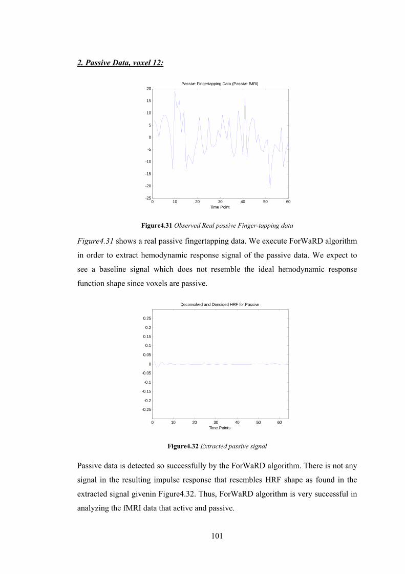
101

2. Passive Data, voxel 12:

0 10 20 30 40 50 60-25

-20

-15

-10

-5

0

5

10

15

20Passive Fingertapping Data (Passive fMRI)

Time Point

Figure4.31 Observed Real passive Finger-tapping data

Figure4.31 shows a real passive fingertapping data. We execute ForWaRD algorithm

in order to extract hemodynamic response signal of the passive data. We expect to

see a baseline signal which does not resemble the ideal hemodynamic response

function shape since voxels are passive.

0 10 20 30 40 50 60

-0.25

-0.2

-0.15

-0.1

-0.05

0

0.05

0.1

0.15

0.2

0.25

Deconvolved and Denoised HRF for Passive

Time Points

Figure4.32 Extracted passive signal

Passive data is detected so successfully by the ForWaRD algorithm. There is not any

signal in the resulting impulse response that resembles HRF shape as found in the

extracted signal givenin Figure4.32. Thus, ForWaRD algorithm is very successful in

analyzing the fMRI data that active and passive.

102

4.2.1.3 Experiment 3: HRF Results of Real Data obtained from specified fMR adaptation paradigm

The third experiment is an fMR adaptation paradigm consisting of 177 time samples,

investigating subtle effects in face processing. Active and passive voxels in this data

are classified beforehand via the general linear model which served as ‘ground truth’.

Real fMRI data is obtained from an experiment conducted on a 1.5T Siemens

scanner.

We have a special stimulus pattern in here. There is no stimulus for the initial 9 time

points. Then, a block which has 27 time points, is repeated for 6 times. This block

consists of zero for the first 9 time points, then it has ones for last 18 time points.

Stimuli in last 18 time points are divided into two categories. First 9 stimuli belong

to one kind of face category and last 9 stimuli belong to another kind of face

category. As mentioned before, we are analyzing subtle effects in face processing in

this experiment.

Experimental design can be summarized as below:

Task: Block paradigm, face perception: 177 sample points:

9 dummies at the beginning (0)

9 patches (0) ---------------------

9 faces (1) ------------------------

9 faces (2) ------------------------

(this group of 27 samples is repeated 6 times) with 6 dummies trailing at the

end

In this experiment, the subject gets used to seeing the same face image for the first 9

stimulus causing a decrease due to habituation in the responding active voxel.

Afterwards, when a new image is shown as the 10th stimulus without any break, the

brain detects the difference between the earlier images for which it has habituated,

causing an increase in the activation of the voxels responding to the face image.

103

This kind of experiments are classified in adaptation paradigm and it is harder to

obtain HRF from this type of experiment data.. Because 2 different categories are

used in one block of stimulus, activation profile of the voxels do not obey the

standard rise and fall in HRF. The recognition of this profile is difficult and

complicated for HRF extraction algorithms. In this section, we analyzed the

performance of ForWaRD method on HRF extraction with this kind of data.

The following method is used in order to investigate the accuracy of the obtained

HRFs.

• We modeled our ideal hemodynamic response function according to the

gamma function as shown in the Figure4.34a..

• We convolved this ideal HRF with the stimulus pattern of the experiment as

shown in Figure4.34 and determined the ideal fMRI signal shown in

Figure4.34b for this experiment if there was no noise in the system.

• After this process, we convolved the HRF which is obtained by the ForWaRD

method and the stimulus pattern of the experiment, and found the estimated

fMRI signal.

• We finalized the accuracy test by finding the error between ideal and

estimated fMRI signals.

The outcome gave us information about the performance of the ForWaRD method.

Active and passive voxels in both real data are classified beforehand via the general

linear model. Stimulus pattern used in the experiment is shown in Figure4.33.

0 20 40 60 80 100 120 140 160 1800

0.5

1

1.5

Figure4.33 Stimulus pattern of the experiment

104

Ideal Hemodynamic response function shape is modelled according to the gamma

function and shown in Figure4.34(a):

0 2 4 6 8 10 12 14 16 18 20-0.2

0

0.2

0.4

0.6

0.8

1

1.2

Hem

odyn

amic

Res

pons

e S

igna

l Cha

nge(

%)

Time Point

(a)

0 20 40 60 80 100 120 140 160 180 200-1

0

1

2

3

4

5

6

Time Point

BO

LD S

igna

l Cha

nge(

%)

(b)

Figure4.34 Ideal HRF(a) & Ideal fMRI (b)

When we convolve ideal HRF shown in Figure4.34(a) and stimulus pattern shown in

Figure4.33 we obtain ideal fMRI shape shown in Figure4.34(b). In order to

understand ForWaRD performance we will be utilized ideal fMRI, shown in

Figure4.34b

For this fMR adaptation paradigm data set we analyzed how regularization parameter

is related with voxel locations. The underlying data set includes active and passive

voxels which are placed in different locations in the brain shown in Figure 4.35. We

investigate how regularization parameter τ changes for voxels which are in different

locations.

First, regularization parameter τ is calculated for active voxels (blue ones) shown in

Figure 4.35 .For active voxels we have τ=12. Second, we calculate τ for passive

voxels which are red ones in Figure 4.35. We obtain τ=11.6 for passive voxels

In conclusion, values of obtained regularization parameters are close to each other

for active and passive voxels which are located in different geographical places in the

brain. So the regularization parameter τ does not inform us about location of the

voxels. In other words, location of the voxel does not affect the regularization

parameter τ.

105

2030

4050

60

2030

4050

60

-10

0

10

20

30

z

Active(Blue) & Passive(Red) Voxels Coordinates

xy

Figure4. 35–Active and Passive vozel locations in the brain

τ=11.6

τ=12

106


1. Active Data, voxel 137

0 20 40 60 80 100 120 140 160 180520

540

560

580fMRI Signal

0 20 40 60 80 100 120 140 160 180-40

-20

0

20Normalized fMRI Signal

Time Points

Figure4.36 a) Original real fMRI data and b) normalized version of the underlying one

The original active fMRI data is shown in Figure4.36a. We normalize the original

data because of its computational advantage which is shown in Figure4.36b. We

deconvolve and denoise the real fMRI signal with ForWaRD method and obtain

hemodynamic response function signal for Active Data 137. HRF Result is shown in

Figure4.37 and comparisons with ideal data are shown in Figure4.38.

0 20 40 60 80 100 120 140 160 180-0.15

-0.1

-0.05

0

0.05

0.1

0.15

0.2

0.25

0.3

0.35Extracted HRF

Time Point


107

HRF in Figure4.37 is extracted by ForWaRD algorithm. The HRF shape resembles

the ideal HRF model. The main difference occurred in the 0-3 time point interval.

There is a sharp and fast increase in this interval and at the same time there is too

much noise on the signal. ForWaRD algorithm assumes that HRF is a smooth signal

but when there is too much noise violating this assumption, it cannot catch this

increase cautiously. This is acceptable for such a complicated time series.

Disregarding the beginning, rest of the signal is quite alike the HRF shape; so the

algorithm is able to recover the HRF signal from the fMRI data. An accuracy test is

done in order to understand how well the algorithm has extracted the HRF signal as

shown below.

0 5 10 15 20-0.5

0

0.5Ideal HRF

0 50 100 150 2000

0.5

1Stimulus Pattern

0 50 100 150 200-2

0

2Ideal fMRI

BO

LD C

hang

e (%

)

Time Points

0 10 20 30 40-0.5

0

0.5Extracted HRF

0 50 100 150 2000

0.5

1Stimulus Pattern

0 50 100 150 200-2

0

2Estimated fMRI

Time Points

BO

LD C

hang

e (%

)

Figure4.38 Comparison of ideal and estimated BOLD change

Figure4.38 shows the ideal HRF and ideal fMRI data on the left hand side and

extracted HRF and estimated fMRI data on the right hand side. When we convolve

the ideal hemodynamic response function and stimulus pattern, we obtain ideal fMRI

signal shown in the left hand side of the Figure4.38. In the same way, when the

extracted hemodynamic response function is convolved with the stimulus pattern we

obtain an estimated fMRI signal.

The signal obtained from the convolution of the extracted HRF and the stimulus

pattern is similar to the ideal signal shape shown on the right side of the Figure4.38.

The reason there are 6 blocks in stimulus pattern of the experiment is because

108

activation occurred 6 times in the responding voxels. These 6 activation transitions

can also be seen in the estimated fMRI data. This accuracy test is done in order to

understand how well the algorithm has extracted the HRF signal and estimated fMRI

signal. The results of the test show that ForWaRD algorithm successfully extracts the

hemodynamic response from a complicated very noisy real fMRI signal.

2. Active Data, voxel 100

0 20 40 60 80 100 120 140 160 180440

460

480

500

520fMRI Signal

0 20 40 60 80 100 120 140 160 180-40

-20

0

20

40Normalized fMRI Signal

Time Points

Figure4.39 Original real fMRI data and normalized version of the underlying one

Figure4.39 shows the original active data 100 fMRI signal (Figure4.39a) and its

normalized version (Figure4.39b). We use the normalized original signal in our

computations because of its computational convenience. After executing the

ForWaRD algorithm, we obtain a hemodynamic response which resembles the ideal

one in terms of shape, magnitude and time intervals where peak values occur. The

underlying hemodynamic response function is shown in Figure4.40.

109

0 20 40 60 80 100 120 140 160 180-0.2

-0.1

0

0.1

0.2

0.3

0.4

0.5Extracted HRF

Time Point


The extracted HRF signal shape given in Figure4.40 is purified again as expected

and the obtained waveform is similar to the ideal model which is shown in

Figure4.34(a). ForWaRD method is significantly successful in filtering noise on the

signal but the sharp increase at the beginning could not be detected because the

signal was assumed to be smooth.

0 5 10 15 20-0.5

0

0.5Ideal HRF

0 50 100 150 2000

0.5

1Stimulus Pattern

0 50 100 150 200-2

0

2Ideal fMRI

BO

LD C

hang

e (%

)

Time Points

0 10 20 30 40-0.5

0

0.5Extracted HRF

0 50 100 150 2000

0.5

1Stimulus Pattern

0 50 100 150 200-5

0

5Estimated fMRI

Time Points

BO

LD C

hang

e (%

)

Figure4.41 Comparison of ideal and estimated BOLD change

In figure 4.41, the comparison of ideal and estimated fMRI signals is given. Ideal

fMRI signal shown on the left side of the Figure4.41 is obtained with the convolution

of ideal hemodynamic response and stimulus pattern of this experiment. On the right

hand side, we convolve extracted hemodynamic response function with the same

stimulus pattern and obtain the estimated fMRI signal. The basic reason of the

difference between ideal and estimated fMRI signal is due to using the ideal stimulus

pattern

110

when computing estimated fMRI signal. It is possible that, during the experiment

ideal stimulus pattern may not be given to the patient. The differences between ideal

stimulus pattern and the used one in the experiment cause distortions in the extracted

hemodynamic response which is the result of the ForWaRD algorithm. When this

underlying distorted hemodynamic response is convolved with ideal stimulus pattern,

the obtained estimated fMRI signal becomes distorted and it becomes different from

the ideal one.

3. Passive Data, voxel 280

0 20 40 60 80 100 120 140 160 180700

705

710

715

720

725

730

735

740Passive fMRI Signal

Time Points

Figure4.42 Original passive fMRI signal

Figure4.42 shows a passive data example from the specified fMR adaptation

paradigm. We want to extract the hemodynamic response function of this data with

ForWaRD algorithm. Extracted hemodynamic response is shown in Figure4.43.

0 20 40 60 80 100 120 140 160-1

-0.8

-0.6

-0.4

-0.2

0

0.2

0.4

0.6

0.8

1Deconvolved and Denoised HRF for Passive Data

Time Points

Figure4.43 ForWARD output of passive fMRI data

111

4. Motion Data, voxel 400

Motion data is a type of passive data which correspond to the voxels affected by head

movement. We analyzed this type of data because it can be confused with active

data. We want to understand the strength of ForWaRD method for this type of data.

0 20 40 60 80 100 120 140 160 180775

780

785

790

795

800

805

810

815

820Motion fMRI Signal

Time Points

Figure4.44 Original motion fMRI data

In Figure4.44 one of the data labeled as motion type data is shown. We investigate

the extracted hemodynamic response function of the underlying data. The extracted

hemodynamic response function is shown in Figure4.45.

0 20 40 60 80 100 120 140 160-1

-0.8

-0.6

-0.4

-0.2

0

0.2

0.4

0.6

0.8

1Deconvolved and Denoised HRF for Motion Data

Time Points

Figure4.45 ForWARD output of motion fMRI data

HRF result for motion data is not like those derived from active voxels, it is like

noise. In this case we may say that ForWaRD is a very robust HRF extraction

method against complex data such as motion signal.

112

4.2.2 Clustering Results and Identification of Active and Passive Voxels

4.2.2.1 Clustering Results of Simulated Data Based on the Balloon Model

4.2.2.1.1 Case1: only AWGN noise added In this section, only AWGN noise is added to fMRI signal with different variants as

sigma=4, 8, 12, 16, 20, 30. For each noise variant (sigma value) a 1000 time series

are created. In each data set, 500 signals are set to represent active voxels and the

other 500 is set to represent passive voxels. In the previous section, a sample signal

was chosen for each data set, then hemodynamic response was found, observed and

shown in graphics. But now, data sets are clustered for each variant in order to

measure the behavior of ForWaRD method under noise manipulations. In the end,

one of the clusters is expected to contain active and the other passive voxels.

Sensitivity -the percentage of active voxels being in active cluster- and specificity -

the percentage of passive voxels being in passive cluster- are calculated accordingly.

Clustering results are obtained using Laplacian Eigenmaps algorithm. The inputs of

the underlying Laplacian Eigenmaps algorithm are HRFs extracted in the ForWaRD

step. Our extracted HRF data set is converted to N x T matrix. ( Let N be the voxel

number and T be the time point). Each row of the matrix contains the HRF which is

obtained for one voxel. The outputs of the Laplacian eigenmaps are eigenvalues and

corresponding eigenvectors. According to the results, it is found that first eigenvector

is a constant one so gives no information about characteristic of the data set. Second

and third eigenvectors shows the separation of the active and passive voxels

explicitly. So, we decided to use second and third eigenvectors in fuzzy c means for

clustering data.

1. σ =4

-0.04 -0.03 -0.02 -0.01 0 0.01 0.02 0.03 0.04-0.15

-0.1

-0.05

0

0.05

0.1Active & Passive Data Cluster

eigenvector 1

eige

nvec

tor 2

passiveactive

Figure4.46 Cluster results for noisy simulated fMRI data which has AWGN σ=4

113

Active Voxels

(total number is 500)

Passive voxels

(total number is 500)

Amount of True Detection 500 484

Amount of False Detection 0 16

Figure4.46 represents, cluster result for noisy simulated fMRI data which has

AWGN with variance σ=4. Recall that first, the hemodynamic responses of the

underlying noisy fMRI were obtained by using ForWaRD method. After this phase

the clustering phase is performed where hemodynamic responses are clustered with

the laplacian eigenmaps method. In the end, the amount of true and false detection of

hemodynamic responses of active and passive voxels are calculated.

All of the active voxels are found to be correctly detected when AWGN variance is

4. The measurement for correct detection of active voxels is measured as sensitivity

which is in case %100. The measurement for correct detection of passive voxels

called as specificity so, the spesicificity is %96.8. Thus, for AWGN with variance 4,

laplacian eigenmaps method successfully clustered the data.

2. σ =16:

-0.1 -0.08 -0.06 -0.04 -0.02 0 0.02 0.04 0.06-0.2

-0.15

-0.1

-0.05

0

0.05

0.1


eigenvector 1

eige

nvec

tor 2

passiveactive

Figure4. 47 Cluster results for noisy simulated fMRI data which has AWGN σ=16

114

Active Voxels (total number is 500)

Passive voxels (total number is 500)



In this part, we increased the noise variance from σ =4 to σ =16. When we increased

the noise on the fMRI data, the sensitivity and specificity values are decreased.

Before clustering, we execute ForWaRD algorithm and obtain hemodynamic

response functions for active and passive signals. Increase in noise causes extraction

of distorted hemodynamic response functions. Due to the distortion in hemodynamic

responses, clustering performance of laplacian eigenmaps algorithm is decreased.In

other words, some of the hemodynamic responses for active and passive signals are

confused and they are not correctly detected. Hence the sensitivity which is the

correct detection of hemodynamic responses of active voxels, becomes %96.8 and

the specificity which is the correct detection of hemodynamic responses of passive

voxels, becomes %87.2.

3. σ =30

-0.1 -0.08 -0.06 -0.04 -0.02 0 0.02 0.04 0.06 0.08 0.1-0.15

-0.1

-0.05

0

0.05


eigenvector 1

eige

nvec

tor 2

passiveactive

Figure4.48 Cluster results for noisy simulated fMRI data which has AWGN σ=30

115

Active Voxels (total number is 500)

Passive voxels (total number is 500)



When we highly increased the noise variance, meaning σ =30, the extracted

hemodynamic response functions with ForWaRD algorithm become highly

corrupted. Due to the fact that, the amount of correct detection of hemodynamic

reponse functions for active and passive voxels are dreadfully decreases. We cannot

catch all the hemodynamic response functions for active voxels in the clustering

because in these conditions the extracted hemodynamic response functions’ shapes

are corrupted and resembles the waveform for passive voxels. So, clustering

algorithm confuses the hemodynamic responses of active and passive ones and the

sensitivity and specificity values are decreased to %77.8 and %57.2 respectively.

σ=4 σ=8 σ=16 σ=20 σ=30

Sensitivity 1 0.996 0.968 0.93 0.778

Specificity 0.968 0.936 0.872 0.768 0.572

Table 2 Sensitivity and Specificity values for clustering results of data on which only AWGN noise added

As a result of clustering HRFs for which features are extracted by Laplacian

Embedding and clustering is done by using fuzzy c means, we can see that the active

and passive groups are clustered with a high percentage when sigma increased till 20.

For sigma being 20, we see that actives and passive voxels are confused, and when σ

is 30, the confusion is even bigger and the voxels cannot be grouped anymore in the

correct clusters. The result is that ForWaRD is quite robust against noise. It can

provide sensible results even for high noise values such as σ=16. In order to decrease

116

the performance of ForWaRD against noise, extreme values of noise should be added

to the signal such as with σ=30

4.2.2.1.2 Case 2: Varying Values for AWGN, jitter, drift, lag

In this section, different values of AWGN, jitter noise, drift and lag are added to the

ideal simulated fMRI signal. Each noisy combination signal with all additions is ran

through the ForWaRD algorithm. As an output of this algorithm, the obtained HRF

signals are clustered with fuzzy c means with features coming from Laplacian

Embedding algorithm. Then we observed whether active and passive voxels are

clustered correctly. A data set of 1000 time series is used for this process. There are

500 specific active and 500 passive signals in this data set. Under each graphics, true

and false detection rates are indicated for active and passive voxels.

Also the correct clustering performances of the active and passive voxels are

represented by sensitivity and specificity values, which are shown in Table 2.

Sensitivity is the percentage of active voxels being in active cluster and specificity is

the percentage of passive voxels being in passive cluster.

Performance

Sensitivity Specificity

σ_AWGN = 2; σ_Jitter = 2

σ_Drift = 2; σ_Lag = 8 0.996 0.97


σ_Drift = 2; σ_Lag = 8 1 0.944


σ_Drift = 2; σ_Lag = 8 0.998 0.878


σ_Drift = 2; σ_Lag = 8 1 0.946


σ_Drift = 2; σ_Lag = 8 1 0.914

117


σ_Drift = 4; σ_Lag = 8 1 0.946


σ_Drift = 8; σ_Lag = 8 0,96 0.938


σ_Drift = 16; σ_Lag = 8 0.996 0.92


σ_Drift = 16; σ_Lag = 16 0.998 0.922


σ_Drift = 16; σ_Lag = 16 0.998 0.822


σ_Drift = 16; σ_Lag = 16 0.984 0.714


σ_Drift = 16; σ_Lag = 16

0.852 0.32

Table 3 Sensitivity and Specificity values results for clustering of data on which varying values of

AWGN, jitter, drift, lag

In Table 3 above, AWGN, jitter noise, drift and lag is shown on the simulated data

with different values. Then noisy data is put to ForWaRD algorithm and HRF results

are obtained, HRF results and the simulated passive signal samples are entered into

the clustering algorithm and sensitivity and specificity values are obtained. With this,

the performance of ForWaRD algorithm is observed according to the changing

artifact types.

In the above Table 3, sensitivity and specificity values are provided for various

situations. Data is added with jitter (σ = 2), drift (σ = 2), lag (σ = 8), AWGN values

are changed in the specific part of the Table 3. Related part of the table is shown

below Table 4

118



σ_Drift = 2; σ_Lag = 8 0.996 0.97


σ_Drift = 2; σ_Lag = 8 1 0.944


σ_Drift = 2; σ_Lag = 8 0.998

0.878

Table 4 Sensitivity and Specifity Analysis for Variable σAWGN

Increasing AWGN doesnot affect the percentage of active voxels being in the correct

cluster. Even though σ_AWGN = 8 represents a high noise value, still the active data

remains in the correct cluster. But on the other hand when σ value of AWGN reaches

8, it is observed that the specificity value decreases. This shows us that when noise

increases extensively, passive voxels can get confused with active ones. In other

words, since the clustering algorithm groups HRFs quite close to each other in one

cluster, it also decides about some of the passives which are also similar to these

HRFs. The reason of this may be that HRF magnitudes decreases while noise

increases. Laplacian Eigenmaps extracts similar features for active and passive

HRFs.

When we look at the #4th and #5rd results of Table 5 shown below, we can see that

jitter is changed while AWGN, drift and lag are kept constant. Increase in jitter didn't

affect the sensitivity -the percentage of active voxels being in active cluster- value.

But it decreased the percentage of passive voxels being in the correct cluster with

%0.032. If we think that this percentage corresponds to 2 voxels where there are 500

passive signals in a data set of 1000, it means that clustering these 2 voxels are faulty

with the increase in jitter. In this case, we can say that the system performance is

119

indeed affected by the change in jitter and passive signals get mixed up with actives

with this change.



σ_Drift = 2; σ_Lag = 8 1 0.946


σ_Drift = 2; σ_Lag = 8 1 0.914

Table 5 Sensitivity and Specifity Analysis for Variable σJitter

The parts where AWGN, jitter and lag had constant values are given in Table 6 for

the case where the performance is changing when drift is increased. Even with the

highest value of drift the performance of the system is quite high. At the end of

ForWaRD, active and passive HRFs are grouped in correct clusters with negligible

errors.



σ_Drift = 2; σ_Lag = 8 1 0.946


σ_Drift = 4; σ_Lag = 8 1 0.946


σ_Drift = 8; σ_Lag = 8 0,96 0.938


σ_Drift = 16; σ_Lag = 8 0.996 0.92

Table 6 Sensitivity and Specifity Analysis for Variable σDrift

120



σ_Drift = 16; σ_Lag = 8 0.996 0.92


σ_Drift = 16; σ_Lag = 16 0.998 0.922

Table 7 Sensitivity and Specifity Analysis for Variable σLag

In Table7 is shown the part where lag changes with the constant values of AWGN,

jitter and drift. Lag being increased alone did not even affect the system

performance. The system is robust only to the changes in lag.



σ_Drift = 16; σ_Lag = 16 0.998 0.922


σ_Drift = 16; σ_Lag = 16 0.998 0.822


σ_Drift = 16; σ_Lag = 16 0.984 0.714


σ_Drift = 16; σ_Lag = 16 0.852 0.32

Table 8 Sensitivity and Specifity Analysis for Variable σLag, σDrift, σAWGN and σJitter

121

Table 8 shows the situations where all the artifact values are changed. According to

our previous observations, the increase in a single artifact did not affect the system

performance, much. But when we increase all the artifacts slowly at the same time,

we see that the system performance proportionally gets affected adversely. Since the

hemodynamic responses of active signals are characteristically similar, the

percentage of active voxels grouped in the same cluster did not change so much but

the percentage of passive voxels grouping in the correct cluster is affected

drastically. The main reason of this is jitter and AWGN noise. Even though

ForWaRD is robust against these noises, system performance decreases when

AWGN and jitter are increased together. With the artifacts having the values

σ_AWGN = 16; σ_Jitter = 8; σ_Drift = 16; σ_Lag = 16 added on ideal simulated

fMRI, the observed results are not successful especially specificity is considered.

4.2.2.2 Clustering Results of Real Data Obtained from a Block Design Fingertapping Experiment

After HRF extraction, we cluster through their structural features, the results of the

ForWaRD algorithm, which are the hemodynamic responses. We expect to see active

voxels with meaningful hemodynamic response functions in one cluster and passive

voxels with noise in the other cluster. Consequently, using two algorithms, we

identify active and passive voxels, meaning find activation regions of the brain.

Clustering results of the data are given below.

Figure4.49 Clusters of fingertapping data

122

In Figure4.49 green voxels are active, while red ones are passive. All of the active

voxels are clustered in the same cluster, similarly all passive one are in the passive

cluster. Therefore, our algorithm has 100 % sensitivity and 100 % specificity on the

data of the fingertapping experiment.

The result shows the strength of the Laplacian eigenmaps on clustering and indirectly

the strength of ForWaRD on HRF extraction.

4.2.2.3 Clustering Results of Real Data obtained from specified fMRI adaptation paradigm

For this experiment, using obtained FMRI data, first we examine the HRF of all

voxels and then cluster them. In addition, we estimate the basic shape of the

hemodynamic response in each voxel.

Active and passive voxels in both real data are classified beforehand via general

linear model, which served as ‘ground truth’. Motion voxels are classified by eye

inspection from among voxels that are predicted by GLM as if they are active.

• 180 active voxel

• 150 passive voxel

• 180 motion voxel

The labeled 510 samples are executed with ForWaRD algorithm and then clustered

with Laplacian Eigenmap and fuzzy c-means algorithm. The result is given below.

123

Figure4.50 Clusters of fMR adaptation paradigm

Active voxels are red, passive voxels are yellow and motion voxels are green ones.

According to our clustering method, 177 of 180 labeled active voxels are in the same

cluster, 148 of 150 labeled passive voxels are in the same cluster and 178 of 180

motion voxels are in the same cluster

Consequently, according to Figure4.50 our method has 98.3 % sensitivity and 98.6

% specificity.

124

CHAPTER 5

SENSITIVITY AND PERFORMANCE ANALYSIS

5 SENSITIVITY AND PERFORMANCE ANALYSIS

5.1 Sensitivity and Performance Analysis

In this chapter, our aim is to test our algorithms, ForWaRD and laplacian eigenmaps,

according to their varying algorithm parameters. Changing the system parameters,

we would like to analyze under what conditions our system performance is affected.

We wish to see the sensitivity of our program depending on the changes of the

parameters.

In Chapter 4, we demonstrated that our ForWaRD algorithm extracts successfully

the Hemodynamic Response Functions of different types of data such as; finger-

tapping and categorized face recognition as real data and a complex simulated data,

the success being assessed in terms of sensitivity and specificity values.

In this part, we investigated the best system parameters for our subsystem through

sequential modifications. In order to evaluate the effects of parameters of our work

correctly, we are utilizing simulated data in this Chapter, since the extracted

hemodynamic response functions are the most satisfying ones. In addition to that,

stimulus pattern and the ideal BOLD response curve, which is modeled based on

balloon model, are available, before adding anyone of the noises such as AWGN,

jitter, drift and lag.

In our system, fMRI is first input to the ForWaRD algorithm then the output of this

algorithm extracted HRFs are clustered by the laplacian eigenmaps algorithm. In this

case, the logical approach is to analyze how the algorithms outputs change under

system parameters changes by keeping the analysis in two levels defined by the 2 sub

systems: First, a parameter analysis is performed for ForWaRD algorithm where

fMRI data is first processed. After the sensitivity analysis on this first sub system, we

set parameters to their optimum values. Then keeping these parameters set to their

optimized values, a performance analysis for clustering algorithm is conducted

depending on the changes of clustering parameters.

125

In Chapter 4, a data set with the values AWGN σ=8, jitter σ=8, drift σ=16, lag σ=16

was created and analyzed. We use a random sample from this data set in order to

accomplish the performance analysis explained above. A random sample signal can

be seen in Figure5.1 which is chosen from that data set and used in the analysis

conducted in this chapter.

0 50 100 150 200 25070

80

90

100

110

120

130

Time Points

Data - Noise Additive=8, Noise Jitter = 8, Drift = 16, Delay = 16

Figure5.1 Noisy Simulated Data

The sample in Figure5.1 is an extremely corrupted signal so that we cannot detect

the original simulated fMRI signal by bare eyes. As a reminder the original simulated

fMRI signal and stimulus pattern are shown in Figure5.2

0 50 100 150 200 2500

0.5

1

Stimulus Pattern

Ttime Points

0 50 100 150 200 25095

100

105

110BOLD Response

Ttime Points

Figure5.2 Stimulus pattern and pure simulated fMRI signal

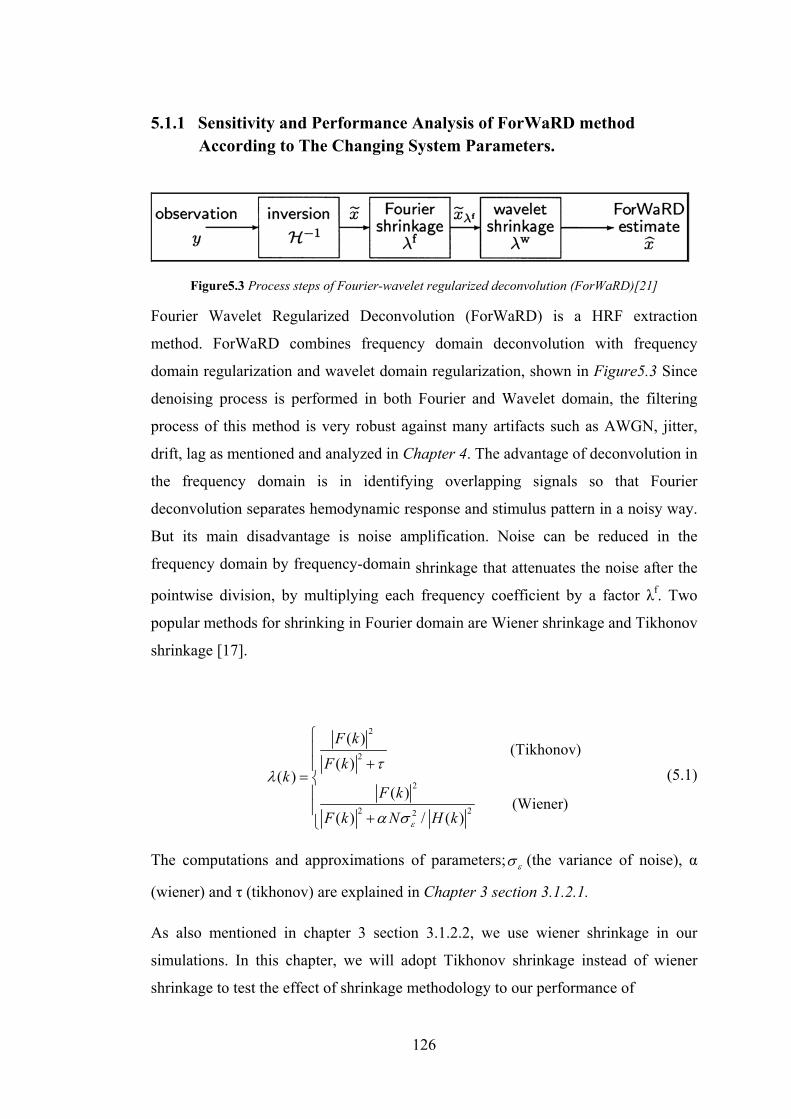
126

5.1.1 Sensitivity and Performance Analysis of ForWaRD method According to The Changing System Parameters.

Figure5.3 Process steps of Fourier-wavelet regularized deconvolution (ForWaRD)[21]

Fourier Wavelet Regularized Deconvolution (ForWaRD) is a HRF extraction

method. ForWaRD combines frequency domain deconvolution with frequency

domain regularization and wavelet domain regularization, shown in Figure5.3 Since

denoising process is performed in both Fourier and Wavelet domain, the filtering

process of this method is very robust against many artifacts such as AWGN, jitter,

drift, lag as mentioned and analyzed in Chapter 4. The advantage of deconvolution in

the frequency domain is in identifying overlapping signals so that Fourier

deconvolution separates hemodynamic response and stimulus pattern in a noisy way.

But its main disadvantage is noise amplification. Noise can be reduced in the

frequency domain by frequency-domain shrinkage that attenuates the noise after the

pointwise division, by multiplying each frequency coefficient by a factor λf. Two

popular methods for shrinking in Fourier domain are Wiener shrinkage and Tikhonov

shrinkage [17].


2

2

2

2 22

( ) (Tikhonov)

( )( )

( ) (Wiener)

( ) / ( )

F kF k

kF k

F k N H kε

τλ

α σ

⎧⎪

+⎪= ⎨

⎪⎪ +⎩

(5.1)

The computations and approximations of parameters; εσ (the variance of noise), α

(wiener) and τ (tikhonov) are explained in Chapter 3 section 3.1.2.1.

As also mentioned in chapter 3 section 3.1.2.2, we use wiener shrinkage in our

simulations. In this chapter, we will adopt Tikhonov shrinkage instead of wiener

shrinkage to test the effect of shrinkage methodology to our performance of

127

ForWaRD. The analyses will be conducted in terms of mean square error (MSE),

calculated between estimated BOLD response (which is convolution of extracted

HRF and stimulus pattern shown in Figure5.2) and original pure BOLD response

shown in Figure5.2.

One of the important parameters is threshold value. In general a small threshold

value will leave behind all the noisy coefficients and subsequently the resultant

denoised image may still be noisy. On the other hand a large threshold value

generates more number of zero coefficients which destroys signal details and the

resultant image begins to have blur and artifacts. So optimum threshold value should

be found out, which is adaptive to different data characteristics. Since the optimum

threshold value changes for each data type, we shall calculate the optimum value for

fMRI data. In this part of the thesis, we will try to find the most suitable threshold for

simulated fMRI data with ForWaRD algorithm.

The other important parameters of ForWaRD are decomposition level and wavelet

basis. The decomposition parameter shows how detailed the separation of this signal

is. The higher the decomposition level, the more detailed coefficients are obtained. In

the wavelet domain, the discrete wavelet transformation only depends on the

maximum decomposition level and the filters (wavelet basis). For a given wavelet

basis, the maximum number of decomposition levels, n, of DWT mainly depends on

the dimensions of the input signals. Maximum decomposition level is computed with

formula below:


max 2 : log ( ), : Maximum Decomposition Level n N N length of data= (5.2)

We will find the optimum level for our simulated data. In addition, mother wavelet

selection is also an important process, so we will examine the changes in system

performance for different mother wavelets and at the end we will decide which one is

best for simulated data.

Briefly; the following settings of the ForWaRD routine will be varied:

128

1. Type of frequency shrinkage:

A) Wiener Shrinkage

B) Tikhonov Shrinkage

2. Wavelet domain threshold level

3. Decomposition levels of wavelet transform

5.1.1.1 Sensitivity Analysis According to the Varying Frequency Shrinkage

In this section, as mentioned before, we tested the performance of the system

according to MSE metric by changing the Fourier Domain Shrinkage method used in

ForWaRD program.

This is how MSE value was calculated: The noisy simulated data given in Figure5.1

was put into ForWaRD algorithm and HRF signal was obtained as the output. Then

this HRF signal was convolved with the stimulus pattern given in Figure5.2. In the

end the MSE value was found by the the difference between ideal BOLD response

given in Figure5.2 and BOLD response as the output of the convolution. Open

formula for MSE is given below.Equation Section (Next)

21 2

1

1 ( )N

i ii

MSE y yN =

= −∑ (5.3)

y1 : ideal BOLD signal

y2 : estimated BOLD signal

i : time point

N : total time point

129

Shrinkage Type

Tikhonov

τ = 1

Tikhonov

τ =5

Tikhonov

τ = 7

Tikhonov

τ = 10

Tikhonov

τ = 20

Tikhonov

τ = 40

Tikhonov

τ = 60

Tikhonov

τ = 100

MSE 1.7235 1.6950 1.6447 1.5952 1.5018 1.4594 1.6366 1.6825

Table 9 MSE comparison for varying Tikhonov regularization parameter τ

Figure5.4 MSE plot versus varying Tikhonov regularization parameter τ

Shrinkage Type

Wiener

=0.01

Wiener

=0.1

Wiener

=1

Wiener

=10

Wiener

=50

MSE 1.7143 1.6115 1.4185 1.4324 1.4706

Table 10 MSE comparison for varying Wiener regularization parameter α

130

Figure5. 5 MSE plot versus varying Wiener regularization parameter α

From Table9 and Table10, Tikhonow shrinkage is found to provide the best MSE

value while regularization parameter τ = 40. When τ gets bigger than 40, MSE starts

to increase. The reason of this is that even though most of the noise is cleared,

because the regularization parameter is highly increased, the signal is corrupted; the

result is noise free but distorted estimate of HRF. Since HRF is corrupted, as the

outcome of the convolution of obtained HRF and stimulus, a distorted BOLD is

obtained and the MSE value with ideal BOLD is increased.

Regularization parameter is a critical parameter for the denoising process. When it is

kept small in order not to corrupt the HRF signal, noise component leaks into the

desired signal HRF, and the result is distortion free but noisy estimate

As explained in Chapter 3, the reason regularization is done in Fourier domain is to

prevent the amplification on the error during Fourier inversion, when stimulus

pattern is either zero or very close to zero.

There is not so much difference between Tikhonow and Wiener thresholds in term of

the ForWaRD performance Wiener has given relatively better results for our data.

That is why we used wiener shrinkage in our simulations.

131

The regularization process and therefore the decision for the regularization parameter

differs in the signal that is processed. The amount of noise on the signal decides how

much regularization should be made. So even though the best outcome for the

sample data that is used in this chapter is obtained for wiener coefficient =1, this

value can change for different data.

5.1.1.2 Sensitivity Analysis According to the Varying Wavelet Domain Threshold Level

Choice of Threshold: The threshold jdT must be chosen just above the maximum

level of the noise. Assume that we want to estimate f from the X f W= + where W

is a Gaussian white noise of variance of 2σ . Then we should determine a threshold

in order to filter noise coefficients. Towards this objective, firstly define a threshold

factor as in equation (5.4) which depends on the data length N. Finally apply hard

threshold to the signal coefficients dj at level j as in equation (5.5) which depends on

both noise variance at level j and threshold factor. j

HarddT is the hard thresholded

signal coefficients at level j The overall threshold t at level j becomes as in equation

(5.6)


( 2)*loge Nρ β= + (5.4)


1,

0, j

j jHardd

j j

if dT

if d

ρσ

ρσ

⎧ ⎫>⎪ ⎪= ⎨ ⎬≤⎪ ⎪⎩ ⎭

(5.5)


( 2)*logj j j et Nρσ σ β= = + (5.6)

The reason why we define a threshold factor depending on data length is based on

the structure of Gaussian white noise. The tail of the Gaussian distribution creates

larger amplitude noise coefficients when the sample size increases.

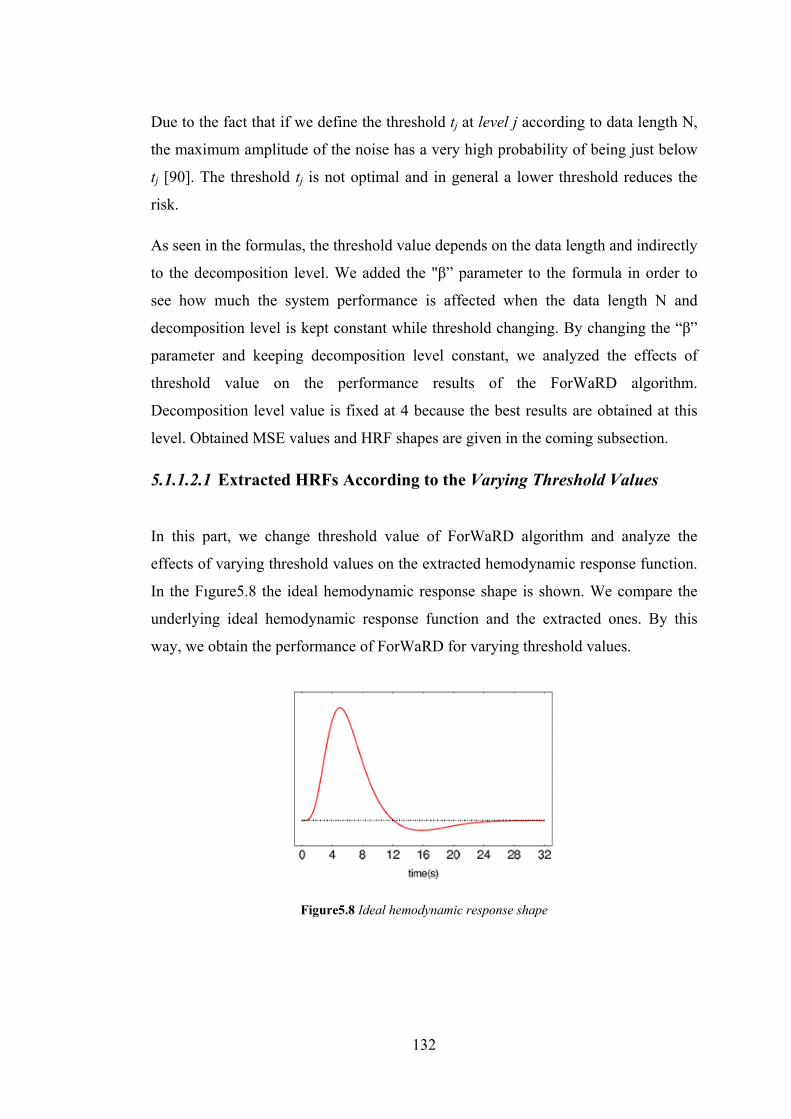
132

Due to the fact that if we define the threshold tj at level j according to data length N,

the maximum amplitude of the noise has a very high probability of being just below

tj [90]. The threshold tj is not optimal and in general a lower threshold reduces the

risk.

As seen in the formulas, the threshold value depends on the data length and indirectly

to the decomposition level. We added the "β” parameter to the formula in order to

see how much the system performance is affected when the data length N and

decomposition level is kept constant while threshold changing. By changing the “β”

parameter and keeping decomposition level constant, we analyzed the effects of

threshold value on the performance results of the ForWaRD algorithm.

Decomposition level value is fixed at 4 because the best results are obtained at this

level. Obtained MSE values and HRF shapes are given in the coming subsection.

5.1.1.2.1 Extracted HRFs According to the Varying Threshold Values

In this part, we change threshold value of ForWaRD algorithm and analyze the

effects of varying threshold values on the extracted hemodynamic response function.

In the Fıgure5.8 the ideal hemodynamic response shape is shown. We compare the

underlying ideal hemodynamic response function and the extracted ones. By this

way, we obtain the performance of ForWaRD for varying threshold values.

Figure5.8 Ideal hemodynamic response shape

133

• Threshold Factor: μ=1 • Threshold Factor : μ=5

0 20 40 60 80 100 120 140 160-6

-4

-2

0

2

4

6


Time Points

Figure5.9 Extracted HRF for Threshold Factor

value μ=1

0 20 40 60 80 100 120 140 160-2

-1.5

-1

-0.5

0

0.5

1

1.5

2


Time Points


value μ=5

For the threshold factor values μ=1 and μ=5, ForWaRD cannot catch the HRF shape

(Figure5.9 and Figure5.10). So, this threshold values are not enough to filter out

noise on the signal at μ=1 and μ=5. When threshold value set to μ=1 and μ=5, then

the noise components disturb more the desired hemodynamic response function

signal components so we can not obtain any meaningful hemodynamic responses

after executing ForWaRD algorithm (Figure5.9 and Figure5.10). When threshold

value is increased from μ=1 to μ=5, noise components filtered more but still we can

not obtain a meaningful hemodynamic response function signal at the threshold value

μ=5 (Figure5.9 and Figure5.10). So, we have to continue to increase threshold value.

134

• Threshold Factor: μ=10 • Threshold Factor : μ=15

0 20 40 60 80 100 120 140 160-0.05

0

0.05

0.1

0.15

0.2

0.25

0.3


Time Points


value μ=10

0 20 40 60 80 100 120 140 160-0.05

0

0.05

0.1

0.15

0.2

0.25


Time Points


value μ=15

In Figure5.11, we can find the extracted hemodynamic response function. When

threshold factor μ value becomes 10 with decomposition level 4, then we obtain the

most identical correspondence between the hemodynamic response function and the

ideal hemodynamic response function shown in Figure5.8. When threshold is μ=10,

ForWaRD filters noise components on the desired hemodynamic response function

very well. Extracted hemodynamic response function shown in Figure5.11 is similar

to ideal hemodynamic response function shown in Figure5.8 in terms of shape,

acceleration when rising and decreasing and time intervals where hemodynamic

response occurs.

When threshold factor value is μ=15 we obtain a satisfying HRF shape according to

the ideal hemodynamic response function shown in Figure5.8. But since the filtered

signal coefficients increase with the increase of threshold level, we can see a

decrease in the signal amplitude. This shows that the threshold level with the value

μ=15 yield to the filtering of some important signal coefficients.

135

• Threshold: μ=20

0 20 40 60 80 100 120 140 160-0.08

-0.06

-0.04

-0.02

0

0.02

0.04

0.06

0.08

0.1


Time Points

Figure5.6 Extracted HRF for Threshold Factor value μ=20

The continuous increase in the threshold level causes HRF to be less ideal when we

compare the extracted hemodynamic response function for threshold value μ=20

shown in the Figure5.13 to the ideal hemodynamic response function shown in the

Figure5.8. Shape of the extracted hemodynamic response shown in the Figure5.13 is

corrupted where the initial peak is not rising smoothly if we compare Figure5.13 to

the ideal hemodynamic response function in the Figure5.8. The reason is that the

signal coefficients in wavelet domain are being filtered by the rising of the threshold.

So, a large threshold value yields more number of zero coefficients of the

hemodynamic response function signal yields which destroys the signal details and

the resultant image yields blur and artifacts. On the other hand, a small threshold

value will leave behind all the noisy coefficients and subsequently the resultant is a

denoised image which may still be noisy.

136

Variable Threshold Factor μ

μ=1 μ=5 μ=10 μ=15 μ=20

Fixed Decomposition

Level n n=4 n=4 n=4 n=4 n=4

MSE 1.7980 1.6279 1.4290 1.4381 1.4602

Table 11 MSE comparison for variable Threshold Factor µ while decomposition level is fixed at 4

Figure5.7 MSE versus Threshold Factor µ

In Table11, MSE comparison for variable Threshold Factor µ while decomposition

level is fixed at 4 is shown. At fixed decomposition level, when the threshold value is

μ=10, we obtain the most satisfying hemodynamic response signal shown in the

Figure5.11 in terms of shape, magnitude and time intervals where hemodynamic

response shape occurred. On the other hand, the graphic of MSE versus Threshold

Factor µ is given in Figure5.14 which shows that the minimum error is obtained

when the threshold factor is μ=10. So, the optimum threshold factor for our

experiment is μ=10, we will use this threshold value in the following analysis.

137

1 2 3 4 5 6 7

μ:1

n:4

μ:5

n:4

μ:10

n:4

μ:13

n:4

μ:15

n: 4

μ:15

n: 4

μ:20

n: 4

Sensitivity (%) 0.75 0.85 0.99 0.96 0.95 0.9 0.88

Specificity (%) 0.68 0.7 0.78 0.74 0.72 0.69 0.69

Table 12 Specificity and Sensitivity analysis for variable threshold factor µ

Briefly in this part, decomposition level value is kept at 4 and threshold value is

changed. The reason decomposition level value is 4 is that, the best results are

obtained at this level. As understood by the HRF shapes and MSE values, when

decomposition level is 4, the best data results are obtained while μ=10 (Figure5.11

and Table 11). Also the results for μ=15 are quite close to the best result shown in

the Figure5.12.

When HRF graphics are observed, the HRFs that are obtained for the best two

threshold values μ=10 shown in the Figure5.11 and μ=15 shown in the Figure5.12

look satisfying in terms of magnitude, shape structure and time intervals where

hemodynamic response function shape occurs.

Another analysis was also made sensitivity and specificity wise shown in the

Table12. Data sets are created with the AWGN σ=8, jitter σ=8, drift σ=16, lag

σ=16 artifact values while decomposition level is constant and threshold value

varying. These datasets, including both active and passive signals, are put into the

ForWaRD algorithm. HRFs that are extracted from ForWaRD are clustered by using

laplacian eigenmaps. As a result of clustering, sensitivity and specificity values are

found. And the best results are obtained when threshold factor is 10. Because when

threshold factor is 10, the successful and decent HRFs shown in the Figure5.11 are

able to be clustered since they look alike characteristically. For other values of

138

threshold factor µ, it was observed that the results had frequent confusions with

passive signals.

These results show us that threshold level is quite an important parameter while

extracting HRF. The settings must be done precisely because the more extracted

HRF shapes get corrupted, the harder it gets for clustering algorithm to separate

active and passive signals.

5.1.1.3 Sensitivity Analysis According to the Varying Decomposition Levels of Wavelet Transform

As explained in the previous analysis, the threshold value changes according to the

decomposition level value. This time ForWaRD performance is analyzed according

to the threshold values which are calculated for non-constant decomposition level

values, while β=15.

ForWaRD can make two types of thresholding in the wavelet domain. These are soft

thresholding and hard thresholding. The open formulas for these threshold shapes are

given in equation (5.7). [89]Equation Section (Next)

( )sgn( ) , ( )

0,

, Hard ( )

0,

softd

hardd

d d t d tSoft Thresholding T d

d t

d d tThresholding T d

d t

⎧ ⎫− >⎪ ⎪→ = ⎨ ⎬≤⎪ ⎪⎩ ⎭

⎧ > ⎫⎪ ⎪→ = ⎨ ⎬≤⎪ ⎪⎩ ⎭

(5.7)

where d is the wavelet coefficient. In soft thresholding the remaining coefficient are

reduced by an amount equal to the value of the threshold. In hard thresholding the

magnitudes of the wavelet coefficients above the threshold are unchanged.

We analyzed how the ForWaRD performance changes according to these two types

of threshold for the sample data we have.

The results are given in Table 13 both MSE and sensitivity specificity wise. Also

HRF shapes are shown in the figures between Figure5.15 and Figure5.22 for each

threshold type and decomposition level value.

139

n=2 n=3 n=4 n=6 n=8

Threshold Type Soft Hard Soft Hard Soft Hard Soft Hard Soft Hard

MSE 1.6697 1.7296 1.4996 1.5048 1.4310 1.4290 1.4780 1.4494 1.5254 1.4661

Table 13 MSE comparison with respect to variable Decomposition levels with Soft and Hard Thresholds

Figure5.8 MSE versus Decomposition Level n with Soft & Hard Thresholding

The results for Soft threshold are better when decomposition level is less (compare

Figure5.15 and Figure5.16, and compare Figure 5.17 and Figure5.18). The reason

of this is that the details of the signal are less distinct for low decomposition levels.

So if we use Soft threshold for lower decomposition levels, we will be able to keep

the signal information. At this point if we use Hard threshold, we can get rid of the

unwanted parts of the signal more clearly and have more detailed information when

the decomposition level increases.

140

But there is an important point here. We cannot have satisfying results either with

soft or hard thresholding, unless we reach the minimum decomposition level value at

which the signal can be separated while incorporating noise. An example for this can

be seen at decomposition level n=2 shown in the Figure5.15 and Figure 5.16. Since

we do not elaborate the signal enough, the noise and coefficients of the signal cannot

be separated from each other and when one of the threshold methods is used on

wavelet coefficients, important signal coefficients are also filtered which at the end

leads to loosing HRF (Figure5.15 and Figure 5.16). This definitely is an unwanted

situation. In order not to come across such situation, the signal should be elaborated

to a suitable level to apply threshold (Figure5.17 and Figure 5.18). In other words,

firstly the decomposition level value should be roughly determined and later the

threshold value and decomposition level should be set to improve the results.

The best values for our sample data are obtained when decomposition level n=4. At

this level, hard threshold process worked better because of reasons explained in the

previous paragraph.

• Decomposition level n=2

Decomposition Level n=2

Soft Threshold Hard Threshold

0 20 40 60 80 100 120 140 160-1

-0.5

0

0.5

1

1.5


Time Points

Figure5.15 Extracted HRF for Soft Threshold when decomposition level n=2

0 20 40 60 80 100 120 140 160-2

-1.5

-1

-0.5

0

0.5

1

1.5

2

2.5


Time Points

Figure5.16 Extracted HRF for Hard Threshold when decomposition level n=2

In Figure5.15 the extracted hemodynamic response function signal for soft

thresholding is shown and in the Figure5.16 the extracted hemodynamic response

141

function for hard thresholding is shown when decomposition level n=2. We cannot

have any meaningful hemodynamic response function signal results either with soft

or hard thresholding in the Figure5.15 and Figure5.16, because we cannot reach the

minimum decomposition level value at which the signal can be separated while

incorporating noise. So, we have to increase decomposition level in order to reach

the desired hemodynamic response signal.




0 20 40 60 80 100 120 140 160-0.1

-0.05

0

0.05

0.1

0.15

0.2

0.25

0.3


Time Points


0 20 40 60 80 100 120 140 160-0.1

-0.05

0

0.05

0.1

0.15

0.2

0.25

0.3

0.35


Time Points


When decomposition level becomes n=4 we obtain satisfactory hemodynamic

response signals with both soft and hard thresholding, results are shown in the

Figure5.17 for soft thresholding and Figure5.18 for hard thresholding. Extracted

hemodynamic response using soft thresholding has better magnitude level shown in

the Figure5.17 than extracted one using hard thresholding shown in the Figure5.18.

Hard thresholding is to smooth the desired signal because of its structure (formula is

given in equation 5.7). When we compare results shown in the Figure5.17 and

Figure5.18 with the ideal hemodynamic response function signal shown in the

Figure 5.8, we find that, extracted hemodynamic responses is very similar to the

ideal one in terms of shape and acceleration for rising to peak value and decreasing

to the base line.

142




0 20 40 60 80 100 120 140 160-0.03

-0.02

-0.01

0

0.01

0.02

0.03

0.04


Time Points


0 20 40 60 80 100 120 140 160-0.1

-0.05

0

0.05

0.1


Time Points


Figure5.19 and Figure5.20 show the extracted hemodynamic response function

signals for decomposition level n=6. When we compare these results to the previous

ones shown in the Figure5.17 and Figure5.18, it is found that results for

decomposition level n=6 shown in the Figure5.19 and Figure5.20 are corrupted.

When the decomposition level equals to 6 than signal becomes more detailed but the

original structure begins to be more destroyed since we separate a signal into a lot of

decomposition levels with wavelet basis. Then we have to filter the required signal

components to correct the corruption and generate less levels.

1 2 3 4

μ:10

n:2

μ:10

n:4

μ:10

n:6

μ:10

n: 8

Sensitivity(%) 0.7 0.99 0.85 0.66

Specificity(%) 0.6 0.71 0.7 0.56

Table 14 Sensitivity and Specificity analysis for variable decomposition level n with fixed threshold

factor µ

143

Table14 demonstrated smoother analysis made according to the sensitivity and

specificity. Data sets are created with the AWGN σ=8, jitter σ=8, drift σ=16, lag

σ=16 artifact values while decomposition level is varying. These datasets, including

both active and passive signals, are put into the ForWaRD algorithm. HRFs that are

extracted from ForWaRD are clustered by using laplacian eigenmaps. As a result of

clustering shown in the Chapter 4, Section 4.2.2.1, sensitivity and specificity values

are found. And the best results are obtained for decomposition level n=4.

At the end of this part, after all of the analysis with varying ForWaRD parameters we

found all of the optimum parameters for our experiment. The best extracted HRF

result shown in the Figure5.21 for the data we used in this chapter is obtained with

the following parameters:

Fourier Shrinkage Type : Wiener Shrinkage

Decomposition Level n : 4

Threshold Factor µ : 10

Wavelet Basis : Daubechies db2, db3

0 20 40 60 80 100 120 140 160-0.1

-0.05

0

0.05

0.1

0.15

0.2

0.25

0.3

0.35


Time Points

Figure5.9 The best extracted HRF result for data we used in Chapter 5

144

5.1.2 Sensitivity and Performance Analysis of Fuzzy C means Clustering Method According to The Changing System Parameters

In this part, we analyzed the sensitivity and performance of the Laplacian Eigenmaps

algorithm.

Specific data sets are created with the AWGN σ=8, jitter σ=8, drift σ=16, lag σ=16

artifact values. These datasets, including both active and passive signals, are put into

the ForWaRD algorithm. HRFs that are extracted from ForWaRD are clustered by

using laplacian eigenmaps. Various algorithm parameters of Laplacian Eigenmaps

are changed and how this change affects the clustering results, is observed.

Laplacian Eigenmaps algorithm has 3 important system parameters. These are:

• Metric of similarity between the neighboring points: Here is the information

for according to which metric, the closest neighbors will be calculated.

Euclidean distance and cosine similarity which are common are used and

results are observed.

o Euclidean distance is the linear distance between two points and is

given by the Pythagorean formula.

o Cosine similarity is a measure of similarity between two vectors by

measuring the cosine of the angle between these two vectors.

• Nearest neighbors of each voxels within the data set.

The two important parameters mentioned above are changed and the uniform data set

is separated into 2 clusters. These clusters are active and passive voxel clusters.

According to the results, obtained sensitivity and specificity values and specific

graphics are given in the following pages.

In all simulations Cosine distance and 4-6-8 nearest neighbors are used.

145

Euclidean Distance

4 Nearest Neighbor 6 Nearest Neighbor

-0.2 -0.15 -0.1 -0.05 0 0.05 0.1 0.15-0.2

-0.15

-0.1

-0.05

0

0.05

0.1


eigenvector 1

eige

nvec

tor 2

passiveactive

Figure5.10 Clustering Result, Euclidean, 4NN

-0.2 -0.15 -0.1 -0.05 0 0.05 0.1 0.15-0.2

-0.15

-0.1

-0.05

0

0.05

0.1


eigenvector 1

eige

nvec

tor 2

passiveactive

Figure5.11 Clustering Result, Euclidean, 6NN

In the Figure5.10, the clustering result for the created data set is shown. Euclidean

distance and 4 nearest neighbor is used for this clustering in the laplacian eigenmaps

algorithm. Figure5.11 shows the clustering result when Euclidean distance and 6

nearest neighbor is used. In both Figures it is shown that clustering is unsuccessful

because hemodynamic responses can not be separated as active and passive. There is

not any crisp boundary between active and passive clusters where the boundary is

rather fuzzy. The sensitivity and specificity values shown in the Table 15 verifies this

unsuccessful situation.

-0.06 -0.04 -0.02 0 0.02 0.04 0.06 0.08-0.06

-0.04

-0.02

0

0.02

0.04

0.06


eigenvector 1

eige

nvec

tor 2

passiveactive

Figure5.12 Clustering Result, Cosine, 6NN

146

In the Figure5.12, the clustering result of the specific data set is given. Cosine

distance and 6 nearest neighbor is used for this clustering. We can find a boundary

between active and passive clusters in the underlying clustering result shown in the

Figure5.12. When we compare using euclidian distance (Figure5.11) and using

cosine distance (Figure5.12) with the same nearest neighbor value, we obtain that

using cosine distance is by far more successful than using Euclidean distance.

Euclidian,

4NN

Euclidian,

6NN Euclidian,

8NN

Sensitivity

(%)

256/553

0.512

254/584

0.508

251/547

0.502

Specificity

(%)

203/447

0.406

169/416

0.338

205/453

0.41

Table 15-Sensitivity and Specificity analyses with respect to Euclidean Dist. and Nearest Neighbor

When Euclidean Distance is used according to the obtained results shown in the

Table15, it is observed that the most significative sample set can be determined by

looking at the 8 nearest neighbors. On the other hand, the most sensitive sample set

can be seen with the nearest 4 neighbors. When analyzed in general, sensitivity

values are quite close to each other for all 4-6-8 neighbors. Sensitivity and specificity

values are not satisfying when found by Euclidian distance. Active and passive

signals could not be separated.

Cosine,

4NN Cosine,

6NN Cosine,

8NN

Sensitivity (%) 492/631

0.984

494/638

0.988

494/630

0.988

Specificity (%) 361/369

0.722

356/362

0.712

364/370

0.728

Table 16 Sensitivity and Specificity analyses with respect to Cosine Distance and Nearest Neighbor

147

When Cosine similarity is used according to the obtained results Table 16, it is

observed that the most significative sample set can be determined by looking at the 8

nearest neighbors. Results seem to be quite close to each other when evaluated

sensitivity wise. It is understood that Cosine distance is a strong metric in separating

active and passive signals from each other. In the end, Cosine similarity is more

successful than Euclidean distance.

148

CHAPTER 6

DISCUSSIONS

6 DISCUSSIONS

6.1 Performance Comparison of ForWaRD and Blind Deconvolution

6.1.1 ForWaRD and Blind Deconvolution In this section, we compared two different model-free approaches for identifying

brain activations from fMRI signals by estimating the underlying hemodynamic

response function (HRF) and interpreting shape features of the obtained HRF

through clustering:

1. Fourier Wavelet Regularized Deconvolution (ForWaRD)

2. Maximum A Posteriori (MAP) Blind Deconvolution

For the purpose of HRF extraction we compared our method to a different

deconvolution technique called MAP blind deconvolution. Following HRF extraction

using ForWaRD, we used Laplacian Eigenmaps algorithm and, for HRF extraction

based on blind deconvolution we used spectral clustering with expectation

maximization (EM) for clustering hemodynamic response functions in order to detect

activation.

We explain maximum a posteriori (MAP) blind deconvolution method briefly in the

following subsection.

6.1.1.1 Maximum A Posteriori (MAP) Blind Deconvolution

The problem is presented as follows:

( ) ( ) ( ) ( )r t d t k t n t= ⊗ +

where,

r(t): Observed fMRI signal,

d(t): Hemodynamic response function.

149

k(t): Stimulus pattern

n(t): Additive White Gaussian noise (AWGN)

Maximum A Posteriori (MAP) Blind Deconvolution technique in which we assume

the fMRI signal is the convolution of HRF with a convolution filter under an

Additive White Gaussian noise (AWGN). We made application dependent

assumptions and formulated them mathematically as prior distributions in order to

cope with the ill-posed nature of blind deconvolution. Because of the slowness of the

hemodynamic response to the neural activation and the averaging of the signal within

the entire neural space of a voxel, we assumed ‘smoothness’ of HRF. Smoothness

constraint on the hemodynamic response implies, in our model, the minimization of

the square sum of derivatives and this turns out to be a Gaussian prior, which favors

high probabilities to low derivative magnitudes. Also, for the convolution filter we

assume it to be of finite impulse response (FIR) of some length p with positive taps:

r(t): Observed fMRI signal, p(r) = Cr

d(t): Hemodynamic response function. 2

1

)(ddT

d−∑−

= eCp d

k(t): Finite Impulse Response (FIR) convolution filter

p(k) = Ck such that ∀i k(i) ≥ 0

n(t): AWGN

By means of MAP approach [1] and the prior distributions we try to minimize the

posterior distribution:

(d * , k * ) = arg m in ( d , k ) − log p r k, d( )p d, k( ){ }

This optimization problem basically tries to approximate the observed signal as a

convolution of d and k while at the same time having the hemodynamic d as smooth

as possible. Unfortunately we face with joint optimization problem in this solution

and we always obtain flat signal for optimum HRF. To tackle this problem, we

modify the solution above using an iterative optimization of the same cost function

through the Expectation-Maximization Algorithm (EM) by basically alternating

150

between the optimum hemodynamic given the convolution filter and the optimum

convolution filter given the hemodynamic. With the help of EM algorithm, we can

avoid the joint optimization and get a suboptimal solution for the same optimization

problem avoiding the flat hemodynamic problem.

The length of the convolution filter p is important. If p is full length we estimate the

HRF. If we choose a suitable and rather smaller p value we obtain a smooth time

series containing both the characteristics of HRF and the information about locations

and durations of the impulses as well. So, these obtained smooth time series signals

are used as input to our clustering algorithm for activation detection meaning that no

further feature extraction is used.

After blind deconvolution, we use spectral clustering with EM for seperating active

and inactive voxels. For a distance measure, we use Hausdorff distance which

outperforms other common distance measures since it is especially robust to the

outliers in the data and able to discard the affect of phase and amplitude shifts among

the signals. Details of this approach are found explicitly in the thesis work [91].

6.1.2 RESULTS

For application first we used simulated data and then we worked with real data. For

the simulated data set we used Balloon Model [3] with parameters ε=0.5, τS= 0.8,

τf= 0.4, τ0= 1, α= 0.2, E0 = 0.8, V0 = 0.02. We discuss the effects of additive noise,

lag, jitter and drift within the data samples.

Real fMRI data set is obtained from a categorical block design experiment. In this

experiment, fMRI data is conducted from a 1.5T Siemens scanner. It is an fMR

adaptation paradigm investigating subtle effects in face processing. Each fMRI data

consist of 177 time points with 6 cycles.

Active and passive voxels in both real data are classified beforehand via general

linear model, which served as ‘ground truth’.

151

6.1.2.1 Hemodynamic Response Function Extraction

6.1.2.1.1 Estimated HRF for Simulated Data

MAP Blind Deconvolution estimates both the HRF and stimulus pattern from a noisy

fMRI data as in Figure6.1 ‘Estimated BOLD response’ refers to the convolution of

the two outputs of the algorithm. Figure6.2 shows the extracted hemodynamic

response using ForWaRD method. ForWaRD method gives better HRF results than

Blind Deconvolution in terms of shape. We loose the initial rise of the HRF when

Blind Deconvolution is used.

Figure6.1 Estimated HRF and stimulus pattern via MAP Blind Deconvolution using simulated data

0 100 200-0.2

0

0.2

0.4

0.6Estimated HRF

0 100 20095

100

105

110Estimated BOLD Response

0 100 200-0.5

0

0.5

1

1.5Stimulus Pattern

0 100 20080

90

100

110

120Observed Signal

Figure6.2 Estimated HRF and stimulus pattern via FORWARD using simulated data

152

6.1.2.1.2 Estimated HRF for Real Data

Figure6.3 and Figure6.4 show the estimated HRF and stimulus pattern for a sample

real fMRI data. In Figure6.3 using Blind Deconvolution, estimated stimulus cannot

detect the last block of the given stimulus pattern. ForWaRD catches the initial rise

of the HRF better than Blind Deconvolution.

Figure6.3 Estimated HRF and stimulus pattern via MAP Blind Deconvolution using real fMRI data

0 50 100 150 200-0.2

0

0.2

0.4Estimated HRF

0 50 100 150 200

-20

0

20

40Estimated BOLD Response

0 50 100 150 200-0.5

0

0.5

1

1.5Stimulus Pattern

0 50 100 150 200-40

-20

0

20

40Observed Signal

Figure6.4 Estimated HRF and stimulus pattern via FORWARD using real fMRI data

153

6.1.2.2 Clustering

In the clustering part we use Spectral Clustering after MAP Blind Deconvolution and

Laplacian eigenmaps after FORWARD method.

6.1.2.2.1 Clustering of Simulated Data

Method1: Blind Deconvolution

Method2: ForWaRD

Table17 shows the performance of both algorithms under different AWGN, lag and

drift artifacts for the simulated data set. Here Table17 gives the standard deviation of

each artifact.

AWGN Lag Quadratic drift

Method1 Method2 Method1 Method2 Method1 Method2

σ=4

Sensitivity 0.998 1 1 0.993 1 0.998

Specificity 0.968 1 0.964 0.992 0.92 0.98

σ=8

Sensitivity 0.998 0.991 0.94 0.962 1 0.976

Specificity 0.938 0.967 0.982 0.945 0.916 0.98

σ=16

Sensitivity 0.956 0.962 1 0.985 1 0.928

Specificity 0.846 0.901 0.888 0.922 0.886 0.932

Table 17 The effect of different noises on the clustering results of both methods

Table18 gives the sensitivity and specificity of each method when all four artifacts

exist within the data with varying standard deviations.

154


Method1 Method2 Method1 Method2

σ_AWGN = 2; σ_Jitter = 2 1 0.996 0.944 0.97


σ_AWGN = 4; σ_Jitter = 2 0.998 1 0.93 0.944


σ_AWGN = 8; σ_Jitter = 2 0.92 0.998 0.942 0.878


σ_AWGN = 4; σ_Jitter = 4 0.96 1 0.962 0.946


σ_AWGN = 4; σ_Jitter = 8 0.912 1 0.954 0.914


σ_AWGN = 4; σ_Jitter = 4 0.998 0.998 0.904 0.922


Table 18 Clustering results under combined noise and lag-drift conditions

Figure6. 5 The illustration of clustering with the simulated data parameters σ_AWGN = 4; σ_Jitter=4 σ_Drift = 16; σ_Lag = 16 using Blind Deconvolution

155

According to Figure6.5, Method1:Blind deconvolution has 99.8 % sensitivity and

90.4 % specificity on the simulated data which has σ_AWGN = 4, σ_Jitter = 4,

σ_Drift = 16, σ_Lag = 16.

Figure6.6 The illustration of clustering with the simulated data parameters σ_AWGN = 4; σ_Jitter=4

σ_Drift = 16; σ_Lag = 16 using Method2

According to Figure6.6, Method2:ForWaRD has 99.8 % sensitivity and 92.2 %

specificity on the simulated data which has σ_AWGN = 4, σ_Jitter = 4, σ_Drift = 16,

σ_Lag = 16.

6.1.2.2.2 Clustering of Real Data

Figure6.7 Clustering of real fMRI data via Method1

156

Method1 obtains 100% performance in both sensitivity and specificity using the

second real fMRI data set as shown in Figure6.7. Active voxels are red, inactive

voxels are blue ones.

Figure6.8 Clustering of real fMRI data via Method2

In Figure6.8, active voxels are red, passive voxels are yellow and motion voxels are

green ones. According to the ForWaRD, sensitivity is 98 % and specificity is 99 %.

6.1.3 CONCLUSIONS

In this work, we basically conducted fMRI data analyses of two types: (1) we

assumed that there is no extra information about the conducted task, and through a

blind deconvolution algorithm within Bayesian framework using a MAP approach,

we estimated the hemodynamic response function. We showed in our analysis that

although this was completely an unsupervised and model free method, we obtained

satisfactory estimates for HRF as well as the unknown stimulus pattern. (2) in order

to further improve our results, we assumed that stimulus is known, By applying the

ForWaRD method, we obtained comparable estimates to the ideal HRF.

Moreover, we also studied Spectral Clustering of fMRI time series using the input

signal as the convolution of estimated HRF and the stimulus estimated from blind

deconvolution under two different settings. Since the distance / similarity metric is

always important for any type of clustering, we analyzed cosine similarity in

ForWaRD method, and the Hausdorff distance in blind deconvolution. In our

157

simulations, we obtained comparable results between these two methods. In case of

blind deconvolution, spectral clustering is followed by an EM clustering in order to

get nice nonlinear boundaries and in case of ForWaRD method, Spectral Clustering

is followed by fuzz-c means which basically assumes Gaussian distribution in data

and declares class memberships accordingly. Since our fMRI simulations assume a

baseline fMRI signal for active class, it tends to generate data having a Gaussian

distribution, which returns favorable results for clustering with fuzz c-means. As for

the real data experiments, clustering after blind deconvolution with Hausdorff

distance outperforms the simulations by generating better sensitivity and specificity

as well as separating the two classes far better in the transformed domain. The reason

behind is that real fMRI signals contain larger within class variability with less

Gaussian distribution with an empowering effect of EM. Moreover, Hausdorff

distance is less sensitive to lags and outliers in signals such as unexpected magnitude

changes in fMRI signals which help much under real life conditions in terms of

clustering.

To sum up with, we obtain a more stable HRF estimations if the stimulus is known

with ForWaRD method, nevertheless, this is not always the case. Whenever HRF is

unpredictable due to variability in cognitve processes, one can still estimate HRF

well and perform a very high quality activation detection through clustering with

Blind Deconvolution.

6.2 Enhancing the Extracted Hemodynamic Response Results for ForWaRD using a Blind Deconvolution Method

In this section, in order to validate the hemodynamic response functions that are

obtained for fMR adaptation paradigm, we crosschecked our results with that of

blind deconvolution which is used obtain hemodynamic response from the same

data.

Blind deconvolution is a method which does not take stimulus pattern as input but

assumes that only fMRI signal is known. Shortly, Blind deconvolution takes the

fMRI signal as input and produces estimated hemodynamic response and estimated

stimulus pattern as output. An example implementation with this approach is

158

provided in [91].

In the previous section, we claimed that the most important reason why the initial

values of hemodynamic response (Figure4.35, Figure 4.38, Figure4.41) does not

include a baseline region might be due to the input given to the ForWaRD algorithm.

What we thought was that during the experiment, a subject might not receive an ideal

stimulus pattern due to interfering sensory and attentional processes. Since the Blind

deconvolution method estimates the actual stimulus pattern perceived by the subject

instead of the ideal stimulus administered by the program, it sets forth a more

realistic stimulus in the output.

When we give the more realistic stimulus pattern -predicted by the Blind

deconvolution method- as input to the ForWaRD algorithm. can we obtain an output

that is closer to the ideal hemodynamic response and retrieve the initial point starting

from a closer point to zero? Using the estimated stimulus pattern for the fMR

adaptation data, “Active Data_100” the result for the ForWaRD estimating a new

hemodynamic response function is given below.

Figure6. 9 HRF Results for Ideal and Estimated Stimulus Patterns

159

As seen in Figure6.9 above, changing the stimulus given to the ForWaRD program

effects the shape of hemodynamic response obtained in the output. The graphics of

hemodynamic response that is obtained by using an ideal stimulus pattern as input

starts from the value 0.3. The initial raise of hemodynamic response is not captured

in this HRF. However, when the stimulus pattern that is estimated with Blind

deconvolution is given to ForWaRD algorithm and the associated hemodynamic

response is obtained, the HRF obtained by using the estimated stimulus is much

closer to the ideal hemodynamic response shape. The initial dip values in the

beginning are caught. So successful results are obtained in the ForWaRD output.

This proves that the most important reason why hemodynamic response functions -

estimated using an ideal stimulus pattern- are inaccurate is because during the

experiment, the actual stimulus pattern that the subject receives is not known and this

stimulus pattern is different than the ideal. Once the input pattern is predicted, the

performance of the ForWaRD program increases drastically.

160

CHAPTER 7

CONCLUSION

The objective of this work was to identify brain activations from fMRI signals by

extracting the underlying hemodynamic response function (HRF) and interpreting

shape features of the obtained HRF through clustering.

In other words, the aim of our study was to identify brain activations so that given a

voxel, we could identify whether there was neural activity in this voxel under a

specific task. We mentioned two sub steps in Chapter 1 and explained in detail how

they can be accomplished to satisfy our goal. We used fMRI signal in form of a time

series signal for each voxel. Unfortunately, for most cases fMRI signals are known to

suffer from low SNR due to several subject/hardware dependent conditions. We

extracted hemodynamic response function (HRF) for every fMRI signal.

Hemodynamic response function (HRF) beared similarity with a system’s impulse

response function, so it was essential for better understanding the underlying neural

activity. In literature survey part of Chapter 2, we mentioned other studies in

literature that are about analyzing fMRI signal.

In general, the relationship between initial neuronal activation and the observed

fMRI rests on a complex physiological process. If this process was known and well

described, it could be approximated by mathematical modeling. However, this

process was still not adequately defined for deriving a model in literature. In

addition, assuming a global model across all voxels of brain is also not realistic. On

the other hand, deconvolution, which is the process of filtering a signal to

compensate for an undesired convolution, was a good alternative approach to address

an intrinsic problem in analyzing desired information. The goal of deconvolution was

to recreate the signal as it existed before the convolution. Deconvolution approach

recovered the fMRI signal as convolution of the underlying HRF with a stimulus

pattern. Since we aimed to unveil the HRF, which was buried within a convolution, a

deconvolution technique was indispensable.

161

In Chapters 2 and 3, we mentioned that the shape features of the obtained HRF

posess information about whether a voxel is “active” or “passive”. After extracting

HRF, in order to identify the activation regions we needed clustering. Chapter 3

deals with the HRF extraction and clustering. We used a simple model-free approach

for this purpose: Fourier Wavelet Regularized Deconvolution (ForWaRD) which

combined frequency-domain deconvolution for identifying overlapping signals,

frequency-domain regularization for suppressing noise, and wavelet-domain

regularization for separating signal and remaining noise. The presented method

ForWaRD, explained in Chapter 3 is attractive, because it requires no knowledge

about the shape of the HRF, and extracting it requires only the fMR image time

series and the stimulus pattern.The output of the ForWaRD algorithm represented the

HRF in every voxel. Application of methods based on ForWaRD to fMRI signal

analysis is a recently studied concept limited to a few articles in the literature. In this

study, the direct ForWaRD method (original method presented in [3]) is applied to

fMRI signals for the first time.

After HRF extraction, fuzzy c-means clustering with Laplacian Embedding

algorithm, called Laplacian eigen maps was used for clustering of active and passive

voxels. Since increasing the dimension of the clustering space leads to practical

difficulties such as “curse of dimensionality” in fuzzy c means algorithm, we

combined this method with laplacian embedding. This includes dimension reduction

of activation data as explained in detail in Chapter 3. Although Laplacian

Embedding or in other terms, manifold based approaches have been tried on fMRI

signal analysis before, to the best of our knowledge, our application of Laplacian

Embedding for classification of extracted HRFs is novel.

In result section of Chapter 4, as a result of ForWaRD algorithm being performed for

block design simulated and real data, extracted HRFs are analyzed. The extracted

HRFs are evaluated both shapewise and magnitudewise. These HRFs are compared

with the ideal HRF model and the difference is observed, the amount of error is

calculated for MSE, specificity and sensitivity. The results showed that ForWaRD

method is very successful in filtering fMRI artifacts (AWGN noise, jitter, drift and

lag) and seperating stimulus from HRF. HRF was successfully obtained even when

fMRI was corrupted with high amount of noise.

162

HRF signals that are obtained by the ForWaRD algorithm are clustered by the

Laplacian eigenmaps algorithm. HRF clustering results obtained from the Laplacian

eigenmaps algorithm gave us important information about performance of both

ForWaRD and clustering. Through the obtained information, we can say ForWaRD

and laplacian eigenmaps methods are successful respectively in obtaining HRF from

fMRI signals and clustering HRFs.

Finally in Chapter 5, sensitivity and performance analysis is performed for both

ForWaRD and Laplacian eigenmaps methods. The aim of this analysis is to observe

how these methods react to changes in system parameters. In this chapter, it is also

shown how and in which values these system parameters are obtained.

In this study of ours, ForWaRD and Laplacian eigemaps algorithms have given quite

satisfying results for block design simulated and real data sets. In the future, this

combination of algorithms should be applied on event related data types and results

should be analyzed in detail.

163

REFERENCES

[1] B Thirion, O Faugeras, Nonlinear Dimension Reduction of FMRI:The

Laplacian Approach, INRIA Sophia Antipolis Odyssee Laboratory, 2004

[2] S. M. SMITH, MA, DPhil, “Overview of fMRI Analysis”

[3] Neelamani R, Choi H, Baraniuk RG: “ForWaRD: Fourier-Wavelet

Regularized Deconvolution for Ill-Conditioned Systems”, IEEE Transactions on

Signal Processing 2004, 52(2):418-433

[4] Prof. Tom O’Haver, “Deconvolution”, Department of Chemistry and

Biochemistry, The University of Maryland at College Park

[5] Tim Edwards, Discrete Wavelet Transforms: Theory and Implementation

[6] Anwei Chai, Zuowei Shen, Deconvolution: A Wavelet Frame Approach

[7] Anat Levin, Yair Weiss, Fredo Durand, William T. Freeman, Understanding

and evaluating blind deconvolution algorithms.

[8] Francis N. Madden, Keith R. Godfrey, Michael J. Chappell, Roman

Hovorka and Ronald A. Bates, “A Comparison of Six Deconvolution Techniques”

[9] Ramesh Neelamani, Hyeokho Choi and Richard Baraniuk, “Wavelet_Based

Deconvolution using Optimally Regularized Inversion for Ill_Conditioned Systems”,

Rice University

[10] Amara Graps,“An Introduction to Wavelets”

[11] Andrew E. Yagle and Byung-Jae Kwak, An Introductıon to Wavelets or: The

Wavelet Transform

[12] Heidelberg Jolliffe, Principal component analysis, IT (1986), Springer. 271 pp.

[13] Roberto Viviani, Georg Gron, and Manfred Spitzer, “Functional Principal

Component Analysis of fMRI Data”

164

[14] K. Sjöstrand1, T. E. Lund, K. H. Madsen, R. Larsen1Sparse, “PCA a new method for unsupervised analyses of fMRI data”

[15] Stephen M. Smith, “Preparing fMRI data for statistical analysis”

[16] R. Tibshirani, "Regression shrinkage and selection via the lasso", Journal of the

Royal Statistical Society - Series B Methodological 58(1), pp. 267-288, 1996.

[17] V. D. Calhoun, T. Adali, L. K. Hansen, J. Larsen, J. J. Pekar, ICA of

Functıonal MRI Data: An Overvıew

[18] J L Marchini and C Heaton, “Applies Spatial ICA (Independent Component

Analysis) to fMRI datasets”

[19] Frithjof Kruggel, and Habib Benali, ICA of fMRI Group Study Data Markus

Svenseń,1

[20] Thomas D. Wickens, “The General Linear Model”, Department of Psychology,

University of California, Berkeley

[21] Alle Meije Wink, Hans Hoogduin and Jos BTM Roerdink, “Data-driven

hemodynamic response function extraction using Fourier-wavelet regularised

deconvolution”

[22] Dimitri Van De Ville,* Thierry Blu, and Michael Unser, “Integrated wavelet

processing and spatial statistical testing of fMRI data” Biomedical Imaging Group,

Swiss Federal Institute of Technology Lausanne (EPFL), [23] E. Gurewitz K. Rose and G. C. Fox., “Vector quantization by deterministic

annealing”

[24] Menon, R.S., Ogawa, S., Strupp, J.P., Anderson, P., Ugurbil, K., 1995.

BOLD based functional MRI at 4 Tesla includes a capillary bed contribution: echo-

planar imaging correlates with previous optical imaging using intrinsic signals.

Magn. Reson. Med. 33, 453– 459.

[25] M. Yang and N. Ahuja, “Gaussian mixture model for human skin color and its

applications in image and video databases”, Technical report, Beckman Institute,

University of Illinois at Urbana-Champaingn, Urbana.

165

[26] Robert E. Greene, “Beyond Frequency Response: A New Approach to Audio Measurement via Wavelets”

[27] Othman O. Khalifa, Sering Habib Harding, “Compression Using Wavelet

Transform”, International Islamic University Malaysia

[28] G. Fung and O. L. Mangasarian, “Semi-supervised support vector machines

for unlabeled data classification. Optimization Methods and Software”, 15(1), April

2001. ftp://ftp.cs.wisc.edu/pub/dmi/tech-reports/99-05.ps.

[29] T. Graepel, “Statistical physics of clustering algorithms”. Technical Report

171822, FB Physik, Institut fur Theoretische Physic, 1998.

[30] K. Chuang and M. Chiu, C. Lin, J. Chen,“Model-free functional MRI analysis

using Kohonen clustering neural network and fuzzy c-means”, IEEE Trans Med

Imag, vol. 18(12), pp.1117-1128, 1999.

[31] M. Fadili, S. Ruan and D. Bloyet, “On the number of clusters and the fuzziness

index for unsupervised FCA application to BOLD fMRI time series”, Medical Image

Analysis, vol. 5(2), pp. 55-67, 2001

[32] M.J. Fadili, S. Ruan, D. Bloyet and B. Mazoyer, “Unsupervised fuzzy

clustering analysis of fMRI series”, proc. of the 20th Annual International Conf. of

IEEE Eng. in Med. & Biol., vol. 20, no. 2, pp. 696-699, 1998

[33] Iain M. Johnstone and Gerard Kerkyacharian, “Wavelet deconvolution in a

periodic setting”, Stanford University, Universite de Paris X-Nanterre Dominique

Picard and Marc Raimondo Universites de Paris VI-VII and University of Sydney

[34] S. Ogawa, “Brain magnetic resonance imaging with contrast dependent on

blood oxygenation”.et al. In Proc. Natl. Acad. Sci. USA, 1990.

[35] Serdar Kemal Balcı, “Classification of Whole Brain fMRI Activation

Patterns”, submitted to the Department of Electrical Engineering and Computer

Science in partial fulfillment of the requirements for the degree of Master of Science

in Electrical Engineering and Computer Science at the MASSACHUSETTS

INSTITUTE OF TECHNOLOGY

166

[36] Roy CS and Sherrington CS, "On the Regulation of the Blood-supply of the

Brain", (January 1890). Journal of Physiology 11 (1-2): 85–158.17. PMID 16991945.

[37] By Ping Bai, Young Truong and Xuemai Huan, “Hemodynamıc Response

Functıon”, University of North Carolina at Chapel Hill

[38] Ogawa, S., Lee, T.M., Nayak, A.S., and Glynn, P.,"Oxygenation-sensitive

contrast in magnetic resonance image of rodent brain at high magnetic fields", (1990)

Magnetic Resonance in Medicine 14: 68–78.

[39] Belliveau JW, Kennedy DN, McKinstry RC, Buchbinder BR, Weisskoff

RM, Cohen MS, Vevea JM, Brady TJ, and Rosen BR, "Functional mapping of the

human visual cortex by magnetic resonance imaging". (1991).Science 254: 716–719.

doi:10.1126/science.1948051. PMID 1948051

[40] Prof. Michael B. Smith, Magnetic Resonance in Medicine (MRM)

[41] KK Kwong, JW Belliveau, DA Chesler, IE Goldberg, RM Weisskoff, BP

Poncelet, DN Kennedy, BE Hoppel, MS Cohen, R Turner, H Cheng, TJ Brady,

and BR Rosen, "Dynamic Magnetic Resonance Imaging of Human Brain Activity

During Primary Sensory Stimulation". (1992) PNAS 89: 5951–55.

doi:10.1073/pnas.89.12.5675.

[42] Jing Xia, Feng Liang and Yongmei Michelle Wang “On Clustering fMRI

Using Potts and Mixture Regression Models”

[43] Bertrand Thirion; Olivier Faugeras, “Activation detection and

characterisation in brain fMRI sequences: Application to the study of monkey

vision”

[44] Ildar Khalidov1, Dimitri Van De Ville1, Jalal Fadili2, and Michael Unser1,

“Activelets and sparsity: A new way to detect brain activation from fMRI data”, 1.

Biomedical Imaging Group, Ecole Polytechnique Fédérale de Lausanne (EPFL),

Switzerland

167

[45] Hamid Soltanian-Zadeh, Gholam- ali Hossein-Zadeg, Babak A.Ardekani, “FMRI Activation Detection in Wavelet Signal Subspace”

[46] David N. Levin and Stephen J. Uftring,“Detecting Brain Activation in FMRI

Data without Prior Knowledge of Mental Event Timing”

[47] Thomas Blumensath, Mike E. Davies, “Iterative Hard Thresholding for

Compressed Sensing”, Institute for Digital Communications & the Joint Research

Institute for Signal and Image Processing

[48] Boon Thye Thomas Yeo and Wanmei Ou, “Clustering fMRI Time Series”,

December 2, 2004

[49] Baumgartner, R., Scarth, G., Teichtmeister, C., Somorjai, R., and Moser,

E. “Fuzzy clustering of gradient-echo functional MRI in the human visual cortex.

Part I: reproducibility”, 1997. J. Magn. Reson.Imag. 7(6): 1094–1101 (see also

Moser et al. 1997).

[50] Baumgartner, R.,Windischberger, C., and Moser, E., “Quantification in

functional magnetic resonance imaging: Fuzzy clustering vs. correlation analysis”,

1998, Magn. Reson. Imag. 16(2): 115–125.

[51] Moser, E., Diemling, M., and Baumgartner R., “Fuzzy clustering of gradient-

echo functional MRI in the human visual cortex. Part II: Quantification”, 1997. J.

Magn. Reson. Imag. 7(6): 1102–1108. For conference with Baumgartner et al. (See

also Baumgartner et al. 1997).

[52] McIntyre, M., Wennerberg, A., Somorjai, R., and Scarth, G. “Activation

and Deactivation in Functional Brain Images.” 1996. In Second International

Conference on Functional Mapping of the Human Brain. (Belliveau et al., Eds.),

NeuroImage 3, 582.

168

[53] Scarth, G., Wennerberg, A., Somorjai, R., Hindermarsh, T., and McIntyre, M., “The Utility of Fuzzy Clustering in Identifying Diverse Activations in fMRI”.

1996. In Second International Conference on Functional Mapping of the Human

Brain. (Belliveau et al., Eds.), NeuroImage 2(2), S89.

[54] Dave´, R. N., and Krishnapuram, R , “Robust clustering methods”: . 1997.

Aunified view. IEEE Trans. Fuzzy Syst. 5(2): 270–293.

[55] Golay, X., Kollias, S., Meier, D., Valavanis, A., and Boesiger “Fuzzy

Membership vs. Probability in Cross Correlation Based Fuzzy Clustering of fMRI

Data”, P. 1997. In Third International Conference on Functional Mapping of the

Human Brain. (Friberg et al., Eds.), NeuroImage 3(3), S481.

[56] Toft, P., Hansen, L. K., Nielsen, F. Å., Goutte, C., Strother, S., Lange, N.,

Mørch, N., Svarer, C., Paulson, O. B., Savoy, R., Rosen, B., Rostrup, E., and

Born, P.”On Clustering of fMRI Time Series”, 1997. In Third International

Conference on Functional Mapping of the Human Brain.

[57] Evgenia Dimitriadou, Markus Barth Christian Windischberger, Kurt

Hornik a Ewald Moser, “A Quantitative Comparison of functional MRI Cluster

Analysis”

[58] Xiong, J., Gao, J.-H., Lancaster, J. L., and Fox, “Assessment and

optimization of functional MRI analyses”. P. T. 1996. Hum. Brain Map.

[59] Worsley, K., and Friston, K.,“Analysis of fMRI time-series revisited”, 1995.

Neuroimage 2: 173–181.

[60] McCullagh, P., and Nelder, J. A., “Generalized Linear Models”, 1989.

Number 37 in Monographs on statistics and applied probability, 2nd ed. Chapman &

Hall, London.

169

[61] Baker, J., Weisskoff, R., Stem, C., Kennedy, D., Jiang, A., Kwong, K.,

Kolodny, L., Davis, T., Boxerman, J., Buchbinder, B., Wedeen, V., Belliveau, J.,

and Rosen B., “Statistical assessment of functional MRI signal change”.

1994.Proceedings of the 2nd Annual Meeting of the Society of Magnetic Resonance,

p. 626

[62] Joset A. Etzel, Valeria Gazzola, Christian Keyser, “An introduction to

anatomical ROI-based fMRI classification analysis”

[63] D. Michie, D.J. Spiegelhalter, C.C. Taylor, “Machine Learning, Neural and

Statistical Classification”, February 17, 1994

[64] James Ford, Hany Farid, Fillia Makedon, Laura A. Flashman, Thomas W.

McAllister, Vasilis Megalooikonomou, and Andrew J. Saykin, “Patient

Classification of fMRI Activation Maps”

[65] Federico De Martino, Giancarlo Valente, Noël Staeren, John Ashburner,

Rainer Goebel and Elia Formisano, “Combining multivariate voxel selection and

support vector machines for mapping and classification of fMRI spatial patterns”

[66] Federico De Martino, Francesco Gentile, Fabrizio Esposito, Marco Balsi,

Francesco Di Salle, Rainer Goebel and Elia Formisano, “Classification of fMRI

independent components using IC-fingerprints and support vector machine

classifiers”

[67] Stephen LaConte, Stephen Strother, Vladimir Cherkassky, Jon Anderson

and Xiaoping Hu, “Support vector machines for temporal classification of block

design fMRI data”

[68] G.P Zhang, “Neural networks for classification: a survey”, Coll. of Bus.,

Georgia State Univ., Atlanta, GA

[69] Eivind Hoffmann, Bureau of Statistics, International Labour Office and

Mary Chamie, “STANDARD STATISTICAL CLASSIFICATIONS: BASIC

PRINCIPLES 11”, United Nations Statistics Division

170

[70] D. Michie, D.J. Spiegelhalter, C.C. Taylor “Machine Learning, Neural and Statistical Classification”, February 17, 1994

[71] Christopher M. Bishop, “Pattern Recognition and Machine Learning”

[72] S. B. Kotsiantis, “Supervised Machine Learning: A Review of Classification

Techniques”

[73] Svetlana V. Shinkareva1,2*, Robert A. Mason1, Vicente L. Malave1, Wei

Wang2, Tom M. Mitchell2, Marcel Adam Just1 “Using fMRI Brain Activation to

Identify Cognitive States Associated with Perception of Tools and Dwellings”

[74] Christos Davatzikos, “Classifying spatial patterns of brain activity with

machine learning methods: application to lie detection”

[75] T. Tony Cai, “Adaptıve Wavelet Estımatıon: A Block Thresholdıng And Oracle

Inequalıty Approach”

[76] Jérôme Kalifa and Stéphane Mallat (2003) “Thresholding estimators for

linear inverse problems and deconvolutions”, Ann. Statist. Volume 31, Number 1,

58-109.

[77] Kalifa, J., Mallat, S. and Rouge, B. (2003), ‘Deconvolution by thresholding in

mirror wavelet bases’, IEEE Transactions on Image Processing 12(4), 446–457.

[78] Sanchez-Avila, C. (2002), ‘Wavelet domain signal deconvolution with

singularity-preserving regularization’, Mathematics and Computers in Simulation

2101, 1–12.

[79] Hillery, A. D. and Chin, R. T. (1991), ‘IterativeWiener filters for image

restoration’, IEEE Transactions on Signal Processing 39, 1892–1899.

[80] Donoho, D. L. and Johnstone, I.M. (1995), ‘Adapting to unknown smoothness

by wavelet shrinkage’, Journal of the American Statistical Association 90, 1200–

1224.

[81] Cai, T. T. (2003), ‘Rates of convergence and adaptation over Besov spaces

under pointwise risk’, Statistica Sinica 13(3), 881–902.

171

[82] Ghael, S. P., Sayeed, A. M. and Baraniuk, R. G. (1997), Improved wavelet

denoising via empirical Wiener filtering, in ‘Proc. SPIE: Wavelet Applications in

Signal and Image Processing’, Vol. 3169, pp. 389–399.

[83] Mallat, S. G. (1989), ‘A theory for multiresolution signal decomposition: The

wavelet representation’, IEEE Transactions on Pattern Analysis and Machine

Intelligence 11(7), 674–693.

[84] Mallat, S. G. (1991), ‘Zero-crossings of a wavelet transform’, IEEE

Transactions on Information Theory 37(4), 1019–1033.

[85] Meyer, F. G. (2003), ‘Wavelet-based estimation of a semiparametric

generalized linear model of fMRI time-series’, IEEE Transactions on Medical

Imaging 22(3), 315–322.

[86]. Buxton RB, Frank LR. A Model for the Coupling Between Cerebral Blood

Flow and Oxygen Metabolism During Neural Stimulation. Journal of Cerebral Blood

Flow and Metabolism, 1997, 17:64-72.

[87] Buxton RB, Wong EC, Frank LR. Dynamics of Blood Flow and Oxygenation

Changes During Brain Activation: The Balloon Model. Magnetic Resonance in

Medicine, 1998, 39:855-864.

[88] Friston KJ, Mechelli A, Turner R, Price CJ. Nonlinear Responses in fMRI: The Balloon Model, Volterra Kernels, and Other Hemodynamics. NeuroImage, 2000, 12:466-477.

[89] Alin Achim, Novel Bayesıan Multiscale Methods For Image Denoising Using

Alpha-Stable Distributions, Doctor of Philosophy at University of Patras, Greece,

June 2003, pp 27.

[90] S.Mallat, A Wavelet Tour of Signal Processing. New York: Academic, 1998

[91] H. İclal Akyol, Blind Deconvolution Based Deconvolution Techniques in

Identifying fMRI Based Brain Activation, METU, 2011

WAVELET BASED DECONVOLUTION TECHNIQUES IN …etd.lib.metu.edu.tr/upload/12613870/index.pdf · submitted by EMİNE ADLI YILMAZ in partial fulfillment of the requirements for ... Performance

Documents