Wastewater life cycle inventory initiative - 2.-0 LCA consultants

Wastewater life cycle inventory initiative

WW LCI version 4.0: model documentation

by Ivan Muñoz 2.-0 LCA consultants, Aalborg, Denmark March 2021

2

Preface

Together with Procter & Gamble, Henkel and Unilever, 2.-0 LCA consultants initiated in 2015 the Wastewater Life Cycle Initiative, with the aim of developing a model to calculate life cycle inventories of chemical substances in wastewater. The Wastewater life cycle initiative is administrated by 2.-0 LCA consultants. For more information and subscription, please contact 2.-0 LCA consultants: http://lca-net.com/clubs/wastewater/ Recommended reference to this report: Muñoz I, (2021), Wastewater life cycle inventory initiative. WW LCI version 4.0: model documentation. 2.-0 LCA consultants, Aalborg, Denmark. http://lca-net.com/clubs/wastewater/ Aalborg, March 2021 Published by: 2.-0 LCA consultants Front page picture: Overview of the wastewater treatment plant of Antwerpen-Zuid, located in the south of the agglomeration of Antwerp (Belgium). Source: https://en.wikipedia.org/wiki/Wastewater_treatment#/media/File:WWTP_Antwerpen-Zuid.jpg

3

C O N T E N T S

Acronyms and abbreviations .................................................................................................................. 8

1 Introduction .................................................................................................................................... 9

2 Goal and scope of WW LCI .............................................................................................................. 11

2.1 Purpose of the model ...................................................................................................................... 11 2.2 Types of substances covered ........................................................................................................... 11 2.3 Types of discharges covered ............................................................................................................ 12 2.4 Tier 1 and Tier 2 assessments .......................................................................................................... 14 2.5 Reference flow ................................................................................................................................. 15 2.6 Boundary with the environment ..................................................................................................... 15 2.7 Life cycle inventory modelling ......................................................................................................... 15 2.8 Background data .............................................................................................................................. 16 2.9 Input data ........................................................................................................................................ 16

2.9.1 Tier 1: wastewater composition .............................................................................................. 16 2.9.2 Tier 2: substance specific data................................................................................................. 16 2.9.3 Scenario data ........................................................................................................................... 17

3 Wastewater and excreta management processes ........................................................................... 19

3.1 Closed sewers .................................................................................................................................. 19 3.1.1 Modelling principles ................................................................................................................ 19 3.1.2 Sewer infrastructure ................................................................................................................ 19 3.1.3 Anaerobic degradation of wastewater in closed sewers ........................................................ 19 3.1.4 Degradation factor for discharges through closed sewers (Degclosed) ..................................... 20

3.2 Open sewers .................................................................................................................................... 24 3.2.1 Modelling principles ................................................................................................................ 24 3.2.2 Identifying open sewers .......................................................................................................... 24 3.2.3 Methane correction factor for open, stagnant sewers (MCFopen) ........................................... 25

3.3 WWTP with secondary treatment – activated sludge ..................................................................... 27 3.3.1 Modelling principles ................................................................................................................ 27 3.3.2 WWTP infrastructure ............................................................................................................... 28 3.3.3 Fate factors .............................................................................................................................. 29 3.3.4 Biological treatment: carbonaceous organic matter removal ................................................ 31 3.3.5 Biological treatment: fate of phosphorus, sulfur and chlorine ............................................... 32 3.3.6 Biological treatment: N2O emissions ....................................................................................... 33 3.3.7 Biological treatment: nutrient consumption ........................................................................... 33

3.4 WWTP with tertiary treatment ....................................................................................................... 34 3.4.1 Modelling principles ................................................................................................................ 34 3.4.2 Biological treatment: carbonaceous organic matter removal ................................................ 35 3.4.3 Biological treatment: nitrogen removal .................................................................................. 35 3.4.4 Biological treatment: nutrient consumption ........................................................................... 37 3.4.5 Phosphorus removal ................................................................................................................ 37 3.4.6 Sand filtration .......................................................................................................................... 38

4

3.4.7 Disinfection .............................................................................................................................. 39 3.5 WWTP with secondary treatment – stabilization pond .................................................................. 40

3.5.1 Modelling principles ................................................................................................................ 40 3.5.2 WWTP infrastructure ............................................................................................................... 41 3.5.3 Fate factors .............................................................................................................................. 42 3.5.4 Biological treatment: carbonaceous organic matter removal ................................................ 44 3.5.5 Biological treatment: nitrogen removal .................................................................................. 44 3.5.6 Anaerobic degradation of settled sludge ................................................................................ 44

3.6 WWTP with primary treatment – conventional .............................................................................. 45 3.6.1 Modelling principles ................................................................................................................ 45 3.6.2 WWTP infrastructure ............................................................................................................... 45 3.6.3 Fate factors .............................................................................................................................. 46

3.7 WWTP with primary treatment – chemically enhanced ................................................................. 48 3.7.1 Modelling principles ................................................................................................................ 48 3.7.2 Fate factors .............................................................................................................................. 48 3.7.3 Phosphorus removal ................................................................................................................ 50 3.7.4 Use of chemicals ...................................................................................................................... 50

3.8 Septic tanks ...................................................................................................................................... 52 3.8.1 Modelling principles ................................................................................................................ 52 3.8.2 Septic tank infrastructure ........................................................................................................ 52 3.8.3 Fate factors .............................................................................................................................. 53 3.8.4 Anaerobic degradation of settled sludge ................................................................................ 54

3.9 Latrines ............................................................................................................................................ 55 3.9.1 Modelling principles ................................................................................................................ 55 3.9.2 Methane correction factor for latrines (MCFlat) ...................................................................... 56

3.10 Open defecation .............................................................................................................................. 56 3.10.1 Modelling principles ................................................................................................................ 57 3.10.2 Methane correction factor for open defecation (MCFdef) ....................................................... 57

4 Wastewater and excreta discharged to the environment ................................................................ 59

4.1 Direct emissions............................................................................................................................... 59 4.2 Indirect emissions ............................................................................................................................ 59

4.2.1 Degradation in the environment ............................................................................................. 60 4.2.2 Methane correction factor for degradation in environmental waters (MCFw) ....................... 62 4.2.3 Methane correction factor for degradation in environmental sediments (MCFsed) ............... 63 4.2.4 Methane emissions.................................................................................................................. 63 4.2.5 Carbon dioxide emissions and carbon sequestration ............................................................. 65 4.2.6 Nitrous oxide emissions ........................................................................................................... 66 4.2.7 Hydrogen sulfide emissions ..................................................................................................... 66 4.2.8 Nitrogen oxides emissions ....................................................................................................... 68 4.2.9 Phosphorus pentoxide emissions ............................................................................................ 68 4.2.10 Hydrogen chloride emissions .................................................................................................. 68 4.2.11 Sulfur oxides emissions ........................................................................................................... 69

5

4.2.12 Nitrate emissions ..................................................................................................................... 69 4.2.13 Phosphate emissions ............................................................................................................... 69 4.2.14 Sulfate emissions ..................................................................................................................... 70 4.2.15 Chloride emissions ................................................................................................................... 71

5 Sludge and septage treatment and disposal .................................................................................... 72

5.1 Sludge and septage treatment ........................................................................................................ 72 5.1.1 Anaerobic digestion of sludge ................................................................................................. 72 5.1.2 Biogas combustion .................................................................................................................. 72 5.1.3 Septage treatment ................................................................................................................... 74 5.1.4 Sludge dewatering ................................................................................................................... 75

5.2 Sludge and septage disposal ............................................................................................................ 75 5.2.1 Sludge composition ................................................................................................................. 75 5.2.2 Sludge transport ...................................................................................................................... 76 5.2.3 Controlled landfilling of sludge ................................................................................................ 76 5.2.4 Uncontrolled landfilling of sludge ........................................................................................... 77 5.2.5 Incineration of sludge .............................................................................................................. 77 5.2.6 Composting of sludge .............................................................................................................. 79 5.2.7 Application of sludge and compost in agriculture ................................................................... 81 5.2.8 Fate of polyelectrolyte during sludge disposal ........................................................................ 83 5.2.9 Uncontrolled septage disposal ................................................................................................ 83

6 Energy balance in WWTPs .............................................................................................................. 84

6.1 Electricity balance ............................................................................................................................ 84 6.1.1 Electricity demand and WWTP size ......................................................................................... 84 6.1.2 Subdivision of electricity demand ........................................................................................... 85 6.1.3 Electricity production .............................................................................................................. 87

6.2 Heat balance .................................................................................................................................... 88 6.2.1 Heat balance model ................................................................................................................. 89 6.2.2 Marginal heat mix .................................................................................................................... 92 6.2.3 Substance-specific heat balance.............................................................................................. 92

7 Wastewater reuse in agriculture .................................................................................................... 95

7.1 Modelling principles ........................................................................................................................ 95 7.2 Emissions from application of wastewater on agricultural land ..................................................... 96 7.3 Substituted irrigation ....................................................................................................................... 97

7.3.1 Irrigation volume ..................................................................................................................... 97 7.3.2 Surface water ........................................................................................................................... 98 7.3.3 Groundwater ........................................................................................................................... 98 7.3.4 Seawater desalination ........................................................................................................... 100

7.4 Substituted crops ........................................................................................................................... 100 7.4.1 Global water intensification factor ........................................................................................ 100 7.4.2 Marginal crop mix .................................................................................................................. 101 7.4.3 Calculation of increased crop production ............................................................................. 103

6

8 Water balance ............................................................................................................................. 105

8.1 Balance for water in wastewater discharges................................................................................. 105 8.2 Balance for water associated to other substances in wastewater discharges .............................. 105

9 Uncertainty ................................................................................................................................. 109

9.1 Basic uncertainty factors ............................................................................................................... 109 9.2 Additional uncertainty via data quality indicators ........................................................................ 111 9.3 Limitations ..................................................................................................................................... 112

10 Linking of inventory data in SimaPro ............................................................................................ 113

10.1 Linking to ecoinvent data sets ....................................................................................................... 113 10.2 Regionalization of water flows ...................................................................................................... 113 10.3 Emission sub-compartments ......................................................................................................... 113

11 Linking of inventory data in GaBi .................................................................................................. 115

11.1 Linking to ecoinvent data sets ....................................................................................................... 115 11.2 Regionalization of water flows ...................................................................................................... 115 11.3 Emission sub-compartments ......................................................................................................... 115

12 WW LCI database ......................................................................................................................... 116

12.1 Wastewater collection and treatment .......................................................................................... 117 12.2 Sludge disposal .............................................................................................................................. 118 12.3 Mean annual and monthly temperatures ..................................................................................... 118 12.4 Wastewater discharge in inland waters ........................................................................................ 118 12.5 Capacity of WWTPs ....................................................................................................................... 119 12.6 Controlled and uncontrolled landfilling of sludge ......................................................................... 119 12.7 Anaerobic digestion and cogeneration in WWTPs ........................................................................ 120 12.8 Methane factors for closed sewers, open sewers and latrines ..................................................... 122 12.9 Open defecation and latrine use ................................................................................................... 123 12.10 Septage disposal ............................................................................................................................ 123 12.11 Wastewater reuse ......................................................................................................................... 125 12.12 Irrigation water supply .................................................................................................................. 125 12.13 Crop production............................................................................................................................. 126 12.14 Secondary wastewater treatment technology .............................................................................. 126 12.15 Stabilization pond capacity ............................................................................................................ 126 12.16 Primary wastewater treatment technology .................................................................................. 126

References ......................................................................................................................................... 128

Appendix 1: Characterization of main wastewater components in a Tier 1 assessment ........................ 138

A1.1 Organic matter, soluble .................................................................................................................... 139 A1.2 Organic matter, suspended .............................................................................................................. 140 A1.3 Ammonium ....................................................................................................................................... 143 A1.4 Phosphate ......................................................................................................................................... 144 A1.5 Sulfate ............................................................................................................................................... 144

7

A1.6 Inert suspended solids...................................................................................................................... 145 A1.7 Water ................................................................................................................................................ 145

Appendix 2: Environmental fate of organic matter in urban wastewater ............................................. 146

Appendix 3: Nitrogen fertilizer ........................................................................................................... 148

8

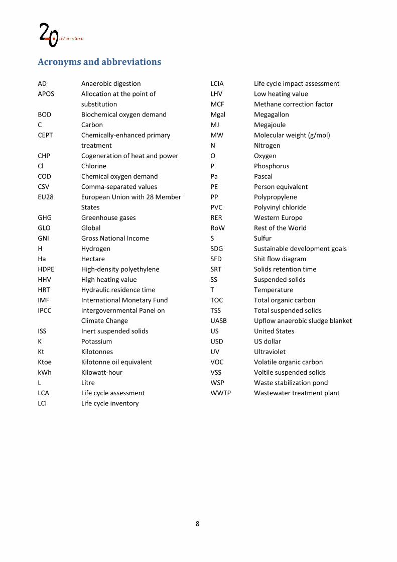
Acronyms and abbreviations

AD Anaerobic digestion APOS Allocation at the point of

substitution BOD Biochemical oxygen demand C Carbon CEPT Chemically-enhanced primary

treatment CHP Cogeneration of heat and power Cl Chlorine COD Chemical oxygen demand CSV Comma-separated values EU28 European Union with 28 Member

States GHG Greenhouse gases GLO Global GNI Gross National Income H Hydrogen Ha Hectare HDPE High-density polyethylene HHV High heating value HRT Hydraulic residence time IMF International Monetary Fund IPCC Intergovernmental Panel on

Climate Change ISS Inert suspended solids K Potassium Kt Kilotonnes Ktoe Kilotonne oil equivalent kWh Kilowatt-hour L Litre LCA Life cycle assessment LCI Life cycle inventory

LCIA Life cycle impact assessment LHV Low heating value MCF Methane correction factor Mgal Megagallon MJ Megajoule MW Molecular weight (g/mol) N Nitrogen O Oxygen P Phosphorus Pa Pascal PE Person equivalent PP Polypropylene PVC Polyvinyl chloride RER Western Europe RoW Rest of the World S Sulfur SDG Sustainable development goals SFD Shit flow diagram SRT Solids retention time SS Suspended solids T Temperature TOC Total organic carbon TSS Total suspended solids UASB Upflow anaerobic sludge blanket US United States USD US dollar UV Ultraviolet VOC Volatile organic carbon VSS Voltile suspended solids WSP Waste stabilization pond WWTP Wastewater treatment plant

9

1 Introduction

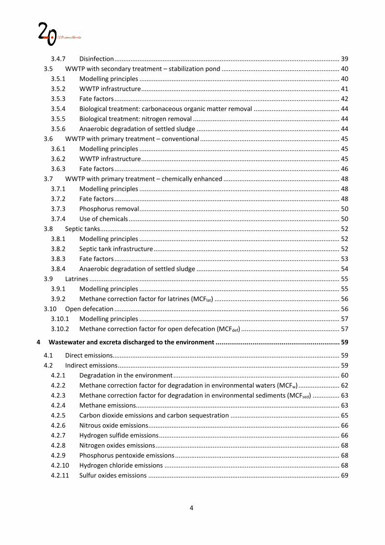
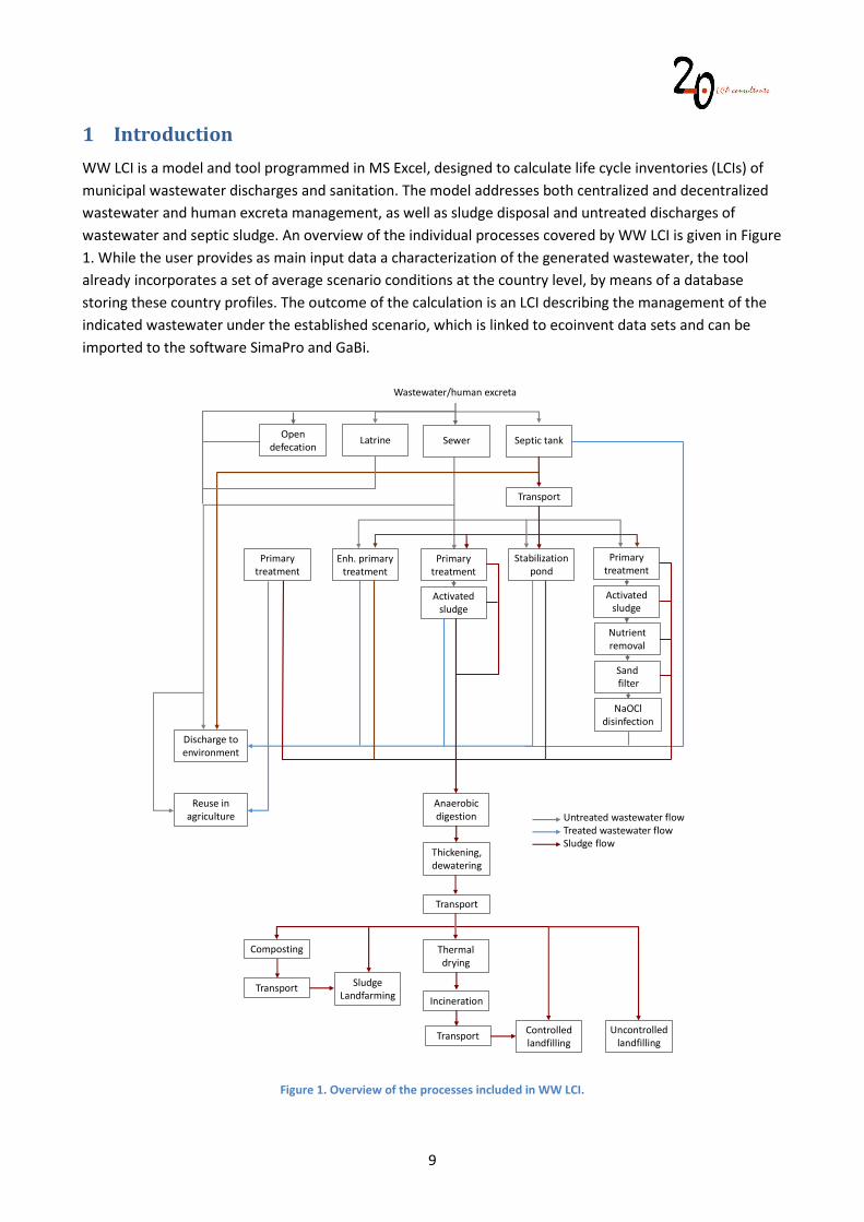
WW LCI is a model and tool programmed in MS Excel, designed to calculate life cycle inventories (LCIs) of municipal wastewater discharges and sanitation. The model addresses both centralized and decentralized wastewater and human excreta management, as well as sludge disposal and untreated discharges of wastewater and septic sludge. An overview of the individual processes covered by WW LCI is given in Figure 1. While the user provides as main input data a characterization of the generated wastewater, the tool already incorporates a set of average scenario conditions at the country level, by means of a database storing these country profiles. The outcome of the calculation is an LCI describing the management of the indicated wastewater under the established scenario, which is linked to ecoinvent data sets and can be imported to the software SimaPro and GaBi.

Figure 1. Overview of the processes included in WW LCI.

Wastewater/human excreta

Discharge to environment

Septic tank

Anaerobic digestion

Sludge Landfarming

Controlled landfilling

Thickening, dewatering

Composting

IncinerationTransport

Transport

Thermal drying

Transport

NaOCldisinfection

Enh. primary treatment

Primary treatment

Activated sludge

Nutrient removal

Activated sludge

Sandfilter

Primary treatment

Untreated wastewater flowTreated wastewater flowSludge flow

Stabilization pond

Sewer

Uncontrolled landfilling

Transport

LatrineOpen defecation

Reuse in agriculture

Primary treatment

10

In this document we provide a complete overview of the latest version of the tool, WW LCI v4. This overview aims to describe in detail the underlying model, data sources and main assumptions. Thus, this document supersedes and updates all previously published material on WW LCI (see Table 1). However, it is not the goal of this report to completely document the model at the mathematical level, but to provide a fair description. All the data, calculations and data sources are traceable in the spreadsheet itself. Also, in this document the actual content of the database storing country-level data is not disclosed, other than in examples used to illustrate how these data are used. A general description of the data sources used to populate the database is provided, though. Table 1. List of previously available documentation on WW LCI that is updated and superseded by this report. Peer-reviewed articles Kalbar P, Muñoz I, Birkved M (2018) WW LCI v2: a second-generation life cycle inventory model for chemicals discharged to

wastewater systems. Sci Total Environ, 622–623: 1649-1657. Muñoz I, Otte N, Van Hoof G, Rigarlsford G (2016) A model and tool to calculate life cycle inventories of chemicals

discharged down the drain. International Journal of Life Cycle Assessment, 22 (6): 986-1004. Conference presentations Muñoz, I (2017) Consequential LCI modeling of chemicals in wastewater: including avoided nutrient treatment. SETAC

Europe 28th Annual Meeting, Barcelona, 27-28 November 2017. Kalbar P, Birkved M, Muñoz I (2017) A second-generation life cycle inventory model for chemicals discharged to

wastewater. SETAC Europe 27th Annual Meeting, Brussels, 7-11 May 2017. Muñoz I, Van Hoof G, Rigarlsford G (2016) LCI model and tool for chemicals discharged down the drain. Case study on

detergent formulations. 22nd SETAC Europe LCA Case Study Symposium, Montpellier, 20-22 September 2016. Muñoz I, Otte N, Van Hoof G, Rigarlsford G (2016) A model and tool to calculate life cycle inventories of chemicals

discharged down the drain. 26th SETAC Europe Annual Meeting, Nantes, 22-26 May 2016. Other documents by 2.-0 LCA consultants Muñoz I (2019) Wastewater life cycle inventory initiative. WW LCI version 3.0: changes and improvements to WW LCI v2. 2.-

0 LCA consultants, Aalborg, Denmark.

11

2 Goal and scope of WW LCI 2.1 Purpose of the model The purpose of WW LCI is to generate LCIs for discharges of chemicals in wastewater, human excreta and wastewater in general. By discharges we refer to the release of the previously mentioned waste to municipal wastewater and sanitation systems, including both centralized and decentralized management. The obtained LCIs can be used to assess or compare end-of-life scenarios for chemical substances used in products or the life-cycle impacts of different wastewater management options, among others. The model is programmed as an Excel spreadsheet that generates the LCIs. With the complementary tool CSVmaker, the LCIs can be converted to comma separated value (csv) files, which can in turn be imported to the software SimaPro and GaBi for further life cycle assessment (LCA) calculations. Currently, WW LCI does not:

Provide results at the life cycle impact assessment (LCIA) level. Results are restricted to the inventory. LCIA results can be obtained by further processing of the LCIs by the user, or by importing them to SimaPro or GaBi, for example.

Specifically address industrial wastewater treatment. However, many of the processes included in WW LCI apply also to industries, such as biological treatment with activated sludge or main sludge disposal practices. In any case, WW LCI can be used to model the discharge of a (treated or untreated) industrial effluent to a municipal wastewater system.

2.2 Types of substances covered WW LCI addresses both organic and inorganic substances. For organic substances, a complete mass flow analysis is conducted for carbon (C), hydrogen (H), oxygen (O), nitrogen (N), phosphorus (P), sulfur (S), and chlorine (Cl). Any other chemical element present in the substance’s composition is accounted for in mass balances, but treated as an inert fraction of the substance’s mass. All chemical conversions involved in wastewater treatment and most of those involved in sludge treatment and disposal are calculated based on stoichiometry, where the following atomic masses are used, in g/mol: C =12, H = 1, O = 16, N = 14, P = 31, S = 32 and Cl =35.5. Besides the coverage of specific chemical substances that can be individually identified as done in e.g. environmental risk assessment, with WW LCI it is also possible to characterise the composition of a wastewater based on generic pollution descriptors, namely:

Chemical oxygen demand (COD) Suspended solids (SS) Total nitrogen (N) Total phosphorus (P)

As for inorganic substances, there is in principle no limitation to the type of substances to be assessed. Specific provisions, however, are built into the model for the following inorganic substances, typically present in wastewater:

Water

12

Ammonium Nitrate Nitrite Phosphate

Nevertheless, as mentioned above, any inorganic substance is in principle in scope. As an example, in Muñoz et al. (2016), WW LCI was used to obtain LCIs for the discharge in wastewater of sodium carbonate, zeolites and sodium tripolyphosphate. Regarding metals, currently WW LCI supports the assessment of the following elements:

Silver Aluminium Arsenic Cadmium Chromium Copper Mercury Manganese Nickel

Lead Zinc Barium Cobalt Iron Magnesium Antimony Vanadium

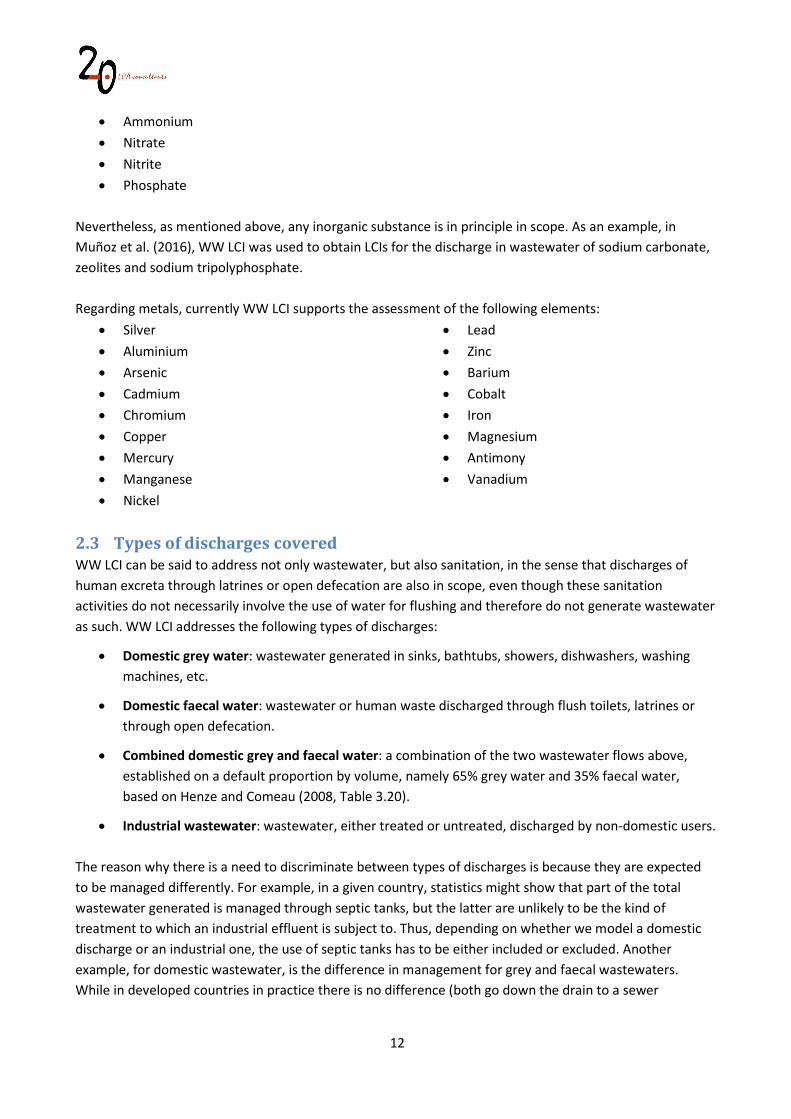
2.3 Types of discharges covered WW LCI can be said to address not only wastewater, but also sanitation, in the sense that discharges of human excreta through latrines or open defecation are also in scope, even though these sanitation activities do not necessarily involve the use of water for flushing and therefore do not generate wastewater as such. WW LCI addresses the following types of discharges:

Domestic grey water: wastewater generated in sinks, bathtubs, showers, dishwashers, washing machines, etc.

Domestic faecal water: wastewater or human waste discharged through flush toilets, latrines or through open defecation.

Combined domestic grey and faecal water: a combination of the two wastewater flows above, established on a default proportion by volume, namely 65% grey water and 35% faecal water, based on Henze and Comeau (2008, Table 3.20).

Industrial wastewater: wastewater, either treated or untreated, discharged by non-domestic users. The reason why there is a need to discriminate between types of discharges is because they are expected to be managed differently. For example, in a given country, statistics might show that part of the total wastewater generated is managed through septic tanks, but the latter are unlikely to be the kind of treatment to which an industrial effluent is subject to. Thus, depending on whether we model a domestic discharge or an industrial one, the use of septic tanks has to be either included or excluded. Another example, for domestic wastewater, is the difference in management for grey and faecal wastewaters. While in developed countries in practice there is no difference (both go down the drain to a sewer

13

connected to a treatment plant), in many developing countries human waste ends up in latrines, while grey water is simply discharged in open drains. These different conditions will affect the inventories in terms of, for example, potential methane emissions, or the environmental compartment receiving the pollution load (surface waters, soil or groundwater). In Table 2 we summarize the management scenarios considered for each one of these types of discharges. Table 2. Management options considered for each type of wastewater discharge in WW LCI.

Management Domestic grey water

Domestic faecal water

Combined domestic grey

and faecal water

Industrial wastewater

Connection to urban wastewater collecting systems No treatment Primary treatment Secondary treatment Tertiary treatment Connection to independent wastewater collecting systems Septic tanks No treatment, discharge No treatment, latrine No treatment, open defecation

In Table 3 we show how discharge scenarios are established in WW LCI, using Kenya as an example. The column with primary data shows the underlying statistics and/or published data found on wastewater management and sanitation for this country, as stored in the WW LCI database. This column does not add up to 100%. This is because the category for ‘No treatment, discharge’ overlaps with the category ‘No treatment, open defecation’ as well as with ‘No treatment, latrine’. Concerning latrines, the table shows no primary data, since this category is calculated as the difference between ‘No treatment, discharge’ and ‘No treatment, open defecation’ for those types of discharges that do consider latrines. The following columns show the calculated discharge scenarios, which result from, as a first step, switching to zero the excluded management options, as shown in Table 2 with ‘’, and as a second step, scaling up the remaining values to 100%. Table 3. Example of calculated discharge scenarios for Kenya in WW LCI.

Wastewater management Primary

data

Types of discharge, calculated from primary data

Domestic, grey water discharge

Domestic, faecal water discharge

Domestic, grey & faecal water discharge

Industrial discharge

Connection to urban wastewater collecting systems - total 19% 19% 19% 19% 23% Urban wastewater collecting systems - without treatment 17% 17% 17% 17% 20% Urban wastewater collecting systems - with treatment 2% 2% 2% 2% 3%

Primary treatment 0% 0% 0% 0% 0% Secondary treatment 2% 2% 2% 2% 3% Tertiary treatment 0% 0% 0% 0% 0%

Connection to independent wastewater collecting systems - total 81% 81% 81% 81% 77% Septic tanks 17% 17% 17% 17% 0% No treatment, discharge 64% 64% 0% 42% 77% No treatment, latrine - 0% 52% 18% 0% No treatment, open defecation 12% 0% 12% 4% 0%

14

It must be borne in mind that the type of discharge ‘Combined domestic grey and faecal water’ has certain limitations. As mentioned above, it splits wastewater into two flows, namely faecal water and grey water, based on their relative volumetric contribution to the total amount of wastewater generated (35% and 65%, respectively). However, the resulting flows are still assumed in the model to have the same chemical composition, which is in practice far from reality for certain parameters. Based on the same source (Henze and Comeau 2008, Table 3.20), faecal water typically contributes with 86% of the total-N and 80% of the total-P, for example. For this reason, this type of discharge should only be used for screening purposes, incurring in potentially highest error in scenarios with relatively high connection to independent wastewater collecting systems. A more accurate modelling in these cases can be achieved by assessing these two flows separately with WW LCI and adding up the resulting inventories manually.

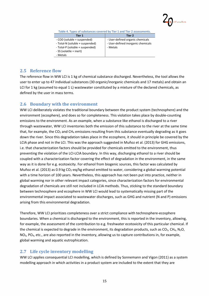
2.4 Tier 1 and Tier 2 assessments The term Tier is used to refer to the level of detail with which the composition of wastewater is defined. WW LCI was designed for LCA practitioners to model chemical substances discharged in wastewater, where the individual substances discharged must be identified, as done in environmental risk assessment. An example would be to assess a wastewater generated by the use of a washing machine, where the individual ingredients in the detergent formulation (content of surfactants A and B, builders C and D, bleaches E and F, water, etc.) are known, as are their proportions in weight. This is an innovative and unique approach, useful for example in LCA studies of consumer products washed down the drain, where this kind of information might be available. When the WW LCI user is in a position to provide data at this level of detail, this is what we call a Tier 2 assessment. Tier 2 in fact corresponds to the traditional way to use WW LCI. A Tier 1 assessment applies when the only information available to the LCA practitioner on wastewater composition is limited to generic pollution descriptors such as chemical oxygen demand (COD). The model accommodates this kind of generic descriptors, for those cases where the individual chemicals present in wastewater cannot be identified. In particular, in Tier 1 a wastewater is defined based on four easily available measures, expressed in mg/L: COD, SS, Total-N and Total-P. A limitation of Tier 1 compared to Tier 2 is that the LCIs obtained with the former do not allow to properly assess toxicity-related impacts from organic pollution in wastewater. This is because the pollution content is described with generic descriptors that are typically excluded from LCIA methods. For example, COD does not have characterization factors for aquatic ecotoxicity. This situation does not occur in Tier 2, since the organic load is in this case specified as a set of individual chemical substances, for which characterization factors might be available. It must be highlighted that in both Tier 1 and Tier 2 assessments, the modelling of the 17 metals is equivalent, based on default fate factors. In Tier 2, however, it is possible to replace these default values by user-specific ones.

15

Table 4. Types of substances covered by Tier 1 and Tier 2 assessments. Tier 1 Tier 2

- COD (soluble + suspended) - User-defined organic chemicals - Total-N (soluble + suspended) - User-defined inorganic chemicals - Total-P (soluble + suspended) - Metals - SS (volatile + inert) - Metals

2.5 Reference flow The reference flow in WW LCI is 1 kg of chemical substance discharged. Nevertheless, the tool allows the user to enter up to 47 individual substances (30 organic/inorganic chemicals and 17 metals) and obtain an LCI for 1 kg (assumed to equal 1 L) wastewater constituted by a mixture of the declared chemicals, as defined by the user in mass terms.

2.6 Boundary with the environment WW LCI deliberately violates the traditional boundary between the product system (technosphere) and the environment (ecosphere), and does so for completeness. This violation takes place by double-counting emissions to the environment. As an example, when a substance like ethanol is discharged to a river through wastewater, WW LCI inventories both the emission of this substance to the river at the same time that, for example, the CO2 and CH4 emissions resulting from this substance eventually degrading as it goes down the river. Since this degradation takes place in the ecosphere, it should in principle be covered by the LCIA phase and not in the LCI. This was the approach suggested in Muñoz et al. (2013) for GHG emissions, i.e. that characterization factors should be provided for chemicals emitted to the environment, thus preventing the violation of the LCI-LCIA boundary. In this way, discharging ethanol to a river should be coupled with a characterization factor covering the effect of degradation in the environment, in the same way as it is done for e.g. ecotoxicity. For ethanol from biogenic sources, this factor was calculated by Muñoz et al. (2013) as 0.9 kg CO2-eq/kg ethanol emitted to water, considering a global warming potential with a time horizon of 100 years. Nevertheless, this approach has not been put into practice, neither in global warming nor in other relevant impact categories, since characterization factors for environmental degradation of chemicals are still not included in LCIA methods. Thus, sticking to the standard boundary between technosphere and ecosphere in WW LCI would lead to systematically missing part of the environmental impact associated to wastewater discharges, such as GHG and nutrient (N and P) emissions arising from this environmental degradation. Therefore, WW LCI prioritizes completeness over a strict compliance with technosphere-ecosphere boundaries. When a chemical is discharged to the environment, this is reported in the inventory, allowing, for example, the assessment of the contribution to e.g. freshwater ecotoxicity of this particular chemical. If the chemical is expected to degrade in the environment, its degradation products, such as CO2, CH4, N2O,

NO3, PO4, etc., are also reported in the inventory, allowing us to capture contributions in, for example, global warming and aquatic eutrophication.

2.7 Life cycle inventory modelling WW LCI applies consequential LCI modelling, which is defined by Sonnemann and Vigon (2011) as a system modelling approach in which activities in a product system are included to the extent that they are

16

expected to change as a consequence of a change in demand for the functional unit. Hence, in consequential modelling what is assessed is a change in demand for the product or service under study. A cause-effect relationship between a change in demand and the related changes in supply is established. This implies that the product is produced by new capacity (if the market trend is increasing). In addition, the affected production capacity must not be constrained, and multifunctionality is dealt with by substitution. The consequential LCI modelling principles are comprehensively described in Weidema et al. (2009) and Weidema (2003). Concerning multifunctionality, wastewater management systems, like many other waste treatment activities, provide more functions than just waste treatment. In particular, wastewater treatment plants (WWTP) may recover energy from biogas, sludge with value as fertilizer or water for irrigation, among others. This is solved by means of substitution (also called system expansion), where by-products displace alternative unconstrained products in a market.

2.8 Background data The background system in WW LCI links to the latest version of the ecoinvent database, in its consequential system model. Data sets are named according to their implementation in the SimaPro software.

2.9 Input data 2.9.1 Tier 1: wastewater composition As already mentioned in previous sections, in a Tier 1 assessment the user can provide the concentration, in mg/L, for COD, total-N, total-P, SS, and for 17 metals. For COD, total-N and total-P it is also possible to specify the dissolved and suspended fractions, while for SS it is possible to specify the volatile and inert fractions, also in mg/L. Appendixes 1 and 2 provide a detailed description of how these parameters are automatically processed by the model to produce a set of wastewater components and environmental fate factors with the same format as in a Tier 2 assessment. 2.9.2 Tier 2: substance specific data A Tier 2 assessment is substantially more data-demanding than a Tier 1 assessment. In this case, a set of physical-chemical properties need to be specified for each chemical substance discharged. The list of potential variables to be defined is the following:

Definition as organic/inorganic Definition as neutral/acid/base Composition in terms of C, H, O, N, S, P and Cl (empirical formula) Molecular weight (g/mol) Carbon origin (biogenic/fossil) Anaerobic degradability (yes/no) Vapor pressure (Pa) Solubility (mg/L) Melting point (ºC) Octanol-water partitioning coefficient (Kow). In case there is no Kow available, it can be replaced by

the solid/liquid partition coefficients in sediments, soil and suspended solids (Kdsed, Kdsoil, Kdsusp). Soil organic carbon-water partitioning coefficient (Koc)

17

Henry’s law constant (Pa·m3/mol) pKa (if applicable) Decay rates in in air, water, sediments and soil (1/s) Fate factors in a WWTP with activated sludge (Fair, Fsludge, Fdeg), namely the fraction of chemical mass

expected to partition to air, to sludge or to degrade, respectively, during treatment in the plant. The remainder is expected as discharged in the treated effluent (Feffluent).

In case the declared substances are being assessed together as a wastewater mixture, it is necessary to define the percentage in mass that each substance constitutes in the mixture.

In practice, not all variables above need to be specified for all substances. Further details on input data are provided in the user manual. 2.9.3 Scenario data By scenario data, we refer to the context or conditions in which wastewater is managed. This includes both geographical conditions (e.g. climate) and technological conditions (sanitation systems in place). By default, scenario data are defined at the country level and include the variables listed below, which are further described in the following chapters of this report.

Wastewater collection and treatment. Establishes the percentage of wastewater or human waste undergoing the following options:

o Collected through a closed sewer and discharged without treatment o Collected through a closed sewer and treated in a WWTP with primary treatment o Collected through a closed sewer and treated in a WWTP with secondary treatment o Collected through a closed sewer and treated in a WWTP with tertiary treatment o Collected through open sewers and discharged without treatment o Collected and treated in a septic tank o Collected through a latrine o Open defecation

WWTP capacity. Establishes the percentage of wastewater treated in five different WWTP capacity classes, and the average capacity (m3/d) in each of these five classes. In addition, it also establishes the average capacity of waste stabilization ponds. This information is used to quantify capital equipment (WWTP and sewer infrastructure), as well as electricity consumption in WWTPs as a function of plant size.

Primary treatment technology. Establishes the percentage of wastewater treated in WWTPs with primary treatment that applies either conventional primary settling or chemically-enhanced primary settling.

Secondary treatment technology. Establishes the percentage of wastewater treated in WWTPs with secondary treatment that applies either activated sludge systems or stabilization pond systems.

Nutrient removal in WWTPs. Establishes the percentage of wastewater that is treated for removal of nitrogen (nitrification-denitrification) and for removal of phosphorus (chemical coagulation). As a default, this is equal to the percentage of wastewater treated in WWTPs with tertiary treatment. It

18

also establishes the percentage of wastewater that is subject to nitrogen removal using methanol as a carbon source. As a default the latter is 0%.

Sludge treatment in WWTPs. Establishes the percentage of wastewater treated in WWTPs with anaerobic digestion of sludge and the percentage of wastewater treated in WWTPs with anaerobic digestion of sludge and cogeneration of heat and power.

Wastewater discharge. Establishes the percentage of wastewater, either treated or untreated, that is discharged to freshwaters or seawaters. Wastewater treated in septic tanks is always assumed to be discharged to groundwaters, while open defecation assumes discharges to soil.

Wastewater reuse. Establishes the percentages of treated and untreated wastewater used for irrigation in agriculture. In countries where water supply for agriculture is not constrained, it also establishes the percentage of freshwater supply from surface water, groundwater and from seawater (produced by desalination). In countries where water supply for agriculture is constrained, a crop production mix is established, reflecting the most likely crops to be affected by a marginal increase in irrigation.

Septic sludge management. Establishes the percentages of septage (sludge removed from septic tanks) that is subject to either safe or unsafe disposal. Safe disposal is modelled as co-treatment with wastewater in a WWTP, while unsafe disposal is modelled as direct discharge to surface waters.

Sludge disposal. Establishes the percentage of sludge disposed of by means of use in agriculture, composting (followed by compost use in agriculture), incineration with energy recovery, controlled landfilling (with biogas and leachate collection and treatment) or uncontrolled landfilling (open dump).

Ambient temperature. Establishes the mean annual and monthly air temperatures. This information is used for the calculation of the heat balance in anaerobic digestion of sludge as well as to estimate methane emissions from open and closed sewers.

Methane correction factors. MCFs reflect the fraction of wastewater degradation that occurs under anaerobic conditions, affecting, among others, methane emissions. We establish MCFs for open/stagnant sewers, direct discharges to surface waters (treated and untreated), latrines, and also for open defecation. For closed sewers we establish a degradation factor expressing the extent of degradation, always assumed to be under anaerobic conditions.

Default country-specific data to populate all these variables is available in the WW LCI database, where all country profiles are stored. These default data, however, can be overridden with user-specific values.

19

3 Wastewater and excreta management processes 3.1 Closed sewers In most developed countries and in high-income urban areas in other countries, sewers are usually closed and underground. 3.1.1 Modelling principles In WW LCI the inventory for substances discharged to closed sewers include the following aspects:

Inputs of sewer infrastructure (section 3.1.2).

Emissions to air associated to anaerobic degradation in the sewer (sections 3.1.3 and 3.1.4).

Emissions to air and water resulting from the discharge of untreated wastewater, when the sewer is not connected to a WWTP (section 4.2).

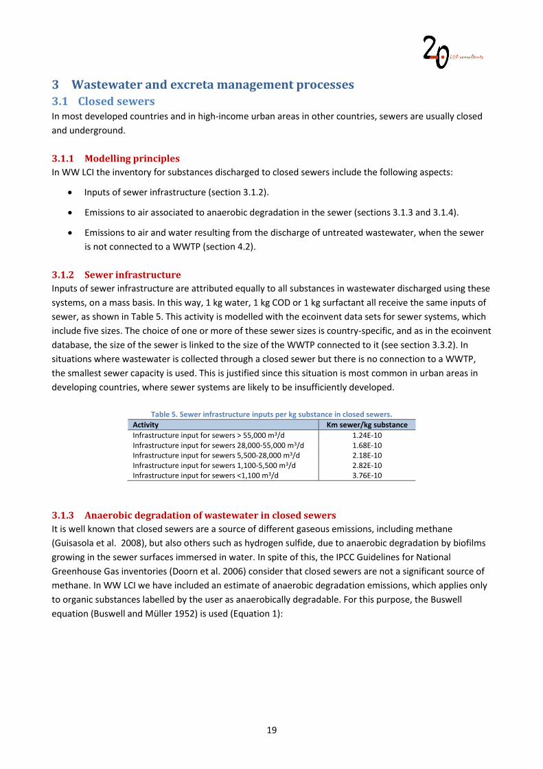
3.1.2 Sewer infrastructure Inputs of sewer infrastructure are attributed equally to all substances in wastewater discharged using these systems, on a mass basis. In this way, 1 kg water, 1 kg COD or 1 kg surfactant all receive the same inputs of sewer, as shown in Table 5. This activity is modelled with the ecoinvent data sets for sewer systems, which include five sizes. The choice of one or more of these sewer sizes is country-specific, and as in the ecoinvent database, the size of the sewer is linked to the size of the WWTP connected to it (see section 3.3.2). In situations where wastewater is collected through a closed sewer but there is no connection to a WWTP, the smallest sewer capacity is used. This is justified since this situation is most common in urban areas in developing countries, where sewer systems are likely to be insufficiently developed.

Table 5. Sewer infrastructure inputs per kg substance in closed sewers. Activity Km sewer/kg substance Infrastructure input for sewers > 55,000 m3/d 1.24E-10 Infrastructure input for sewers 28,000-55,000 m3/d 1.68E-10 Infrastructure input for sewers 5,500-28,000 m3/d 2.18E-10 Infrastructure input for sewers 1,100-5,500 m3/d 2.82E-10 Infrastructure input for sewers <1,100 m3/d 3.76E-10

3.1.3 Anaerobic degradation of wastewater in closed sewers It is well known that closed sewers are a source of different gaseous emissions, including methane (Guisasola et al. 2008), but also others such as hydrogen sulfide, due to anaerobic degradation by biofilms growing in the sewer surfaces immersed in water. In spite of this, the IPCC Guidelines for National Greenhouse Gas inventories (Doorn et al. 2006) consider that closed sewers are not a significant source of methane. In WW LCI we have included an estimate of anaerobic degradation emissions, which applies only to organic substances labelled by the user as anaerobically degradable. For this purpose, the Buswell equation (Buswell and Müller 1952) is used (Equation 1):

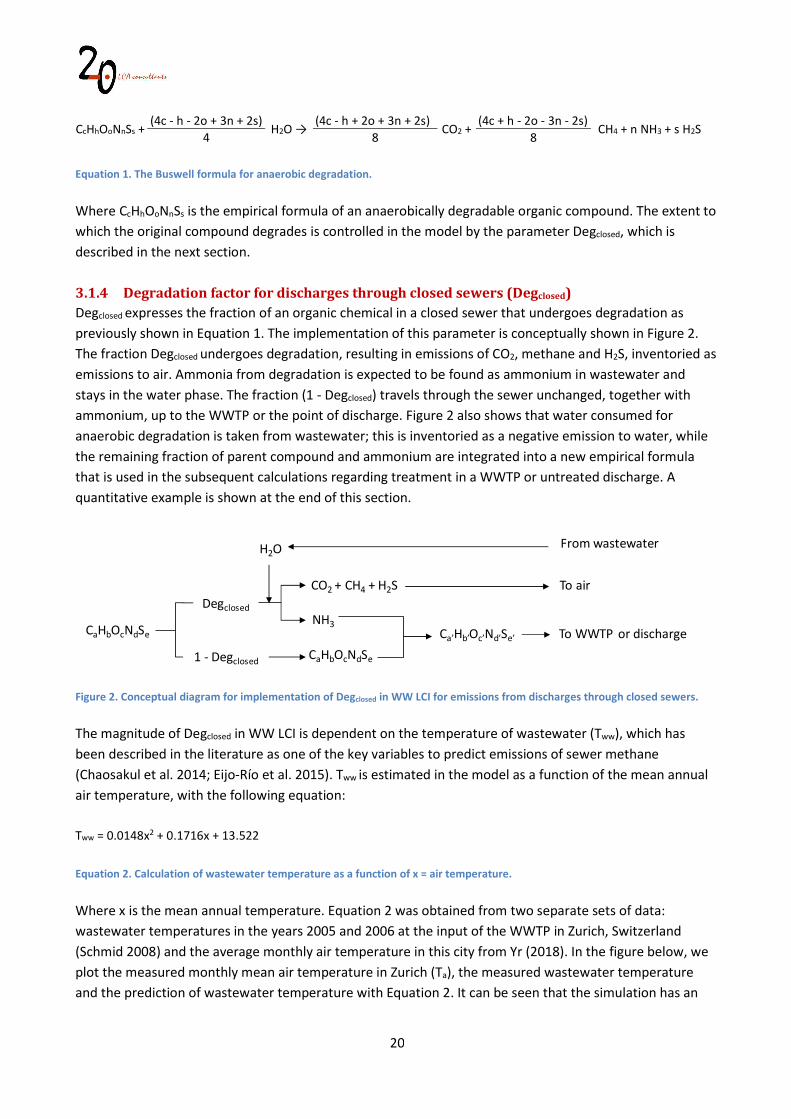
20

CaHbOcNdSe

Degclosed

1 - Degclosed

CO2 + CH4 + H2S To air

H2O

NH3

CaHbOcNdSe

From wastewater

Ca’Hb’Oc’Nd’Se’ To WWTP or discharge

CcHhOoNnSs + (4c - h - 2o + 3n + 2s)

H2O → (4c - h + 2o + 3n + 2s)

CO2 + (4c + h - 2o - 3n - 2s)

CH4 + n NH3 + s H2S 4 8 8

Equation 1. The Buswell formula for anaerobic degradation. Where CcHhOoNnSs is the empirical formula of an anaerobically degradable organic compound. The extent to which the original compound degrades is controlled in the model by the parameter Degclosed, which is described in the next section. 3.1.4 Degradation factor for discharges through closed sewers (Degclosed) Degclosed expresses the fraction of an organic chemical in a closed sewer that undergoes degradation as previously shown in Equation 1. The implementation of this parameter is conceptually shown in Figure 2. The fraction Degclosed undergoes degradation, resulting in emissions of CO2, methane and H2S, inventoried as emissions to air. Ammonia from degradation is expected to be found as ammonium in wastewater and stays in the water phase. The fraction (1 - Degclosed) travels through the sewer unchanged, together with ammonium, up to the WWTP or the point of discharge. Figure 2 also shows that water consumed for anaerobic degradation is taken from wastewater; this is inventoried as a negative emission to water, while the remaining fraction of parent compound and ammonium are integrated into a new empirical formula that is used in the subsequent calculations regarding treatment in a WWTP or untreated discharge. A quantitative example is shown at the end of this section.

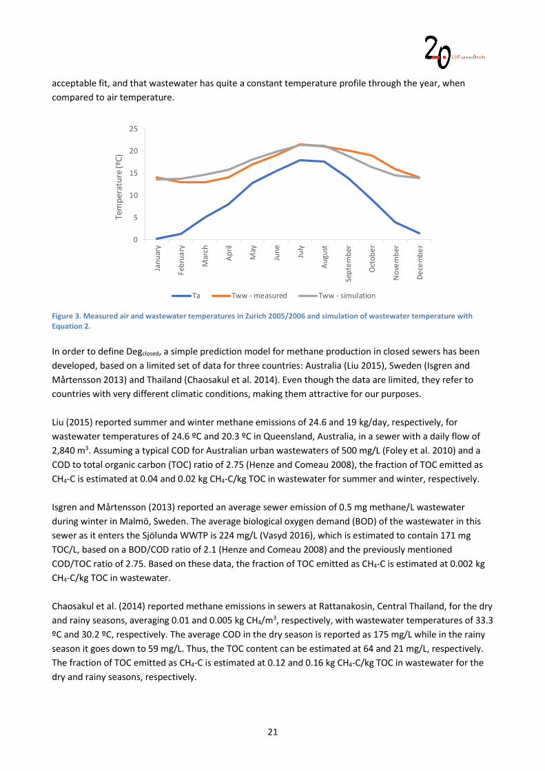
Figure 2. Conceptual diagram for implementation of Degclosed in WW LCI for emissions from discharges through closed sewers. The magnitude of Degclosed in WW LCI is dependent on the temperature of wastewater (Tww), which has been described in the literature as one of the key variables to predict emissions of sewer methane (Chaosakul et al. 2014; Eijo-Río et al. 2015). Tww is estimated in the model as a function of the mean annual air temperature, with the following equation: Tww = 0.0148x2 + 0.1716x + 13.522 Equation 2. Calculation of wastewater temperature as a function of x = air temperature. Where x is the mean annual temperature. Equation 2 was obtained from two separate sets of data: wastewater temperatures in the years 2005 and 2006 at the input of the WWTP in Zurich, Switzerland (Schmid 2008) and the average monthly air temperature in this city from Yr (2018). In the figure below, we plot the measured monthly mean air temperature in Zurich (Ta), the measured wastewater temperature and the prediction of wastewater temperature with Equation 2. It can be seen that the simulation has an

21

acceptable fit, and that wastewater has quite a constant temperature profile through the year, when compared to air temperature.

Figure 3. Measured air and wastewater temperatures in Zurich 2005/2006 and simulation of wastewater temperature with Equation 2. In order to define Degclosed, a simple prediction model for methane production in closed sewers has been developed, based on a limited set of data for three countries: Australia (Liu 2015), Sweden (Isgren and Mårtensson 2013) and Thailand (Chaosakul et al. 2014). Even though the data are limited, they refer to countries with very different climatic conditions, making them attractive for our purposes. Liu (2015) reported summer and winter methane emissions of 24.6 and 19 kg/day, respectively, for wastewater temperatures of 24.6 ºC and 20.3 ºC in Queensland, Australia, in a sewer with a daily flow of 2,840 m3. Assuming a typical COD for Australian urban wastewaters of 500 mg/L (Foley et al. 2010) and a COD to total organic carbon (TOC) ratio of 2.75 (Henze and Comeau 2008), the fraction of TOC emitted as CH4-C is estimated at 0.04 and 0.02 kg CH4-C/kg TOC in wastewater for summer and winter, respectively. Isgren and Mårtensson (2013) reported an average sewer emission of 0.5 mg methane/L wastewater during winter in Malmö, Sweden. The average biological oxygen demand (BOD) of the wastewater in this sewer as it enters the Sjölunda WWTP is 224 mg/L (Vasyd 2016), which is estimated to contain 171 mg TOC/L, based on a BOD/COD ratio of 2.1 (Henze and Comeau 2008) and the previously mentioned COD/TOC ratio of 2.75. Based on these data, the fraction of TOC emitted as CH4-C is estimated at 0.002 kg CH4-C/kg TOC in wastewater. Chaosakul et al. (2014) reported methane emissions in sewers at Rattanakosin, Central Thailand, for the dry and rainy seasons, averaging 0.01 and 0.005 kg CH4/m3, respectively, with wastewater temperatures of 33.3 ºC and 30.2 ºC, respectively. The average COD in the dry season is reported as 175 mg/L while in the rainy season it goes down to 59 mg/L. Thus, the TOC content can be estimated at 64 and 21 mg/L, respectively. The fraction of TOC emitted as CH4-C is estimated at 0.12 and 0.16 kg CH4-C/kg TOC in wastewater for the dry and rainy seasons, respectively.

0

5

10

15

20

25

Janu

ary

Febr

uary

Mar

ch

April

May

June July

Augu

st

Sept

embe

r

Oct

ober

Nov

embe

r

Dece

mbe

r

Tem

pera

ture

(ºC)

Ta Tww - measured Tww - simulation

22

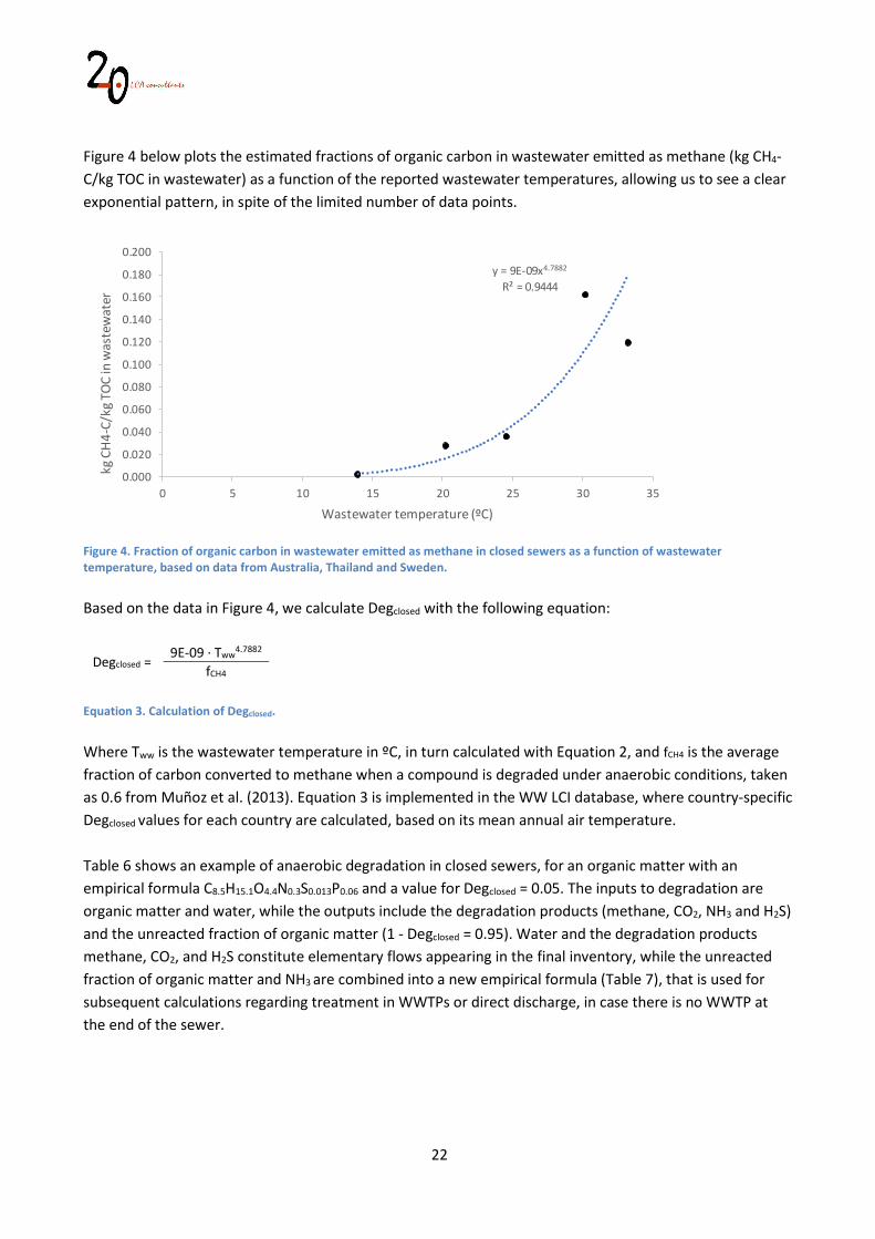
Figure 4 below plots the estimated fractions of organic carbon in wastewater emitted as methane (kg CH4-C/kg TOC in wastewater) as a function of the reported wastewater temperatures, allowing us to see a clear exponential pattern, in spite of the limited number of data points.

Figure 4. Fraction of organic carbon in wastewater emitted as methane in closed sewers as a function of wastewater temperature, based on data from Australia, Thailand and Sweden. Based on the data in Figure 4, we calculate Degclosed with the following equation:

Degclosed = 9E-09 · Tww

4.7882 fCH4

Equation 3. Calculation of Degclosed. Where Tww is the wastewater temperature in ºC, in turn calculated with Equation 2, and fCH4 is the average fraction of carbon converted to methane when a compound is degraded under anaerobic conditions, taken as 0.6 from Muñoz et al. (2013). Equation 3 is implemented in the WW LCI database, where country-specific Degclosed values for each country are calculated, based on its mean annual air temperature. Table 6 shows an example of anaerobic degradation in closed sewers, for an organic matter with an empirical formula C8.5H15.1O4.4N0.3S0.013P0.06 and a value for Degclosed = 0.05. The inputs to degradation are organic matter and water, while the outputs include the degradation products (methane, CO2, NH3 and H2S) and the unreacted fraction of organic matter (1 - Degclosed = 0.95). Water and the degradation products methane, CO2, and H2S constitute elementary flows appearing in the final inventory, while the unreacted fraction of organic matter and NH3 are combined into a new empirical formula (Table 7), that is used for subsequent calculations regarding treatment in WWTPs or direct discharge, in case there is no WWTP at the end of the sewer.

y = 9E-09x4.7882

R² = 0.9444

0.000

0.020

0.040

0.060

0.080

0.100

0.120

0.140

0.160

0.180

0.200

0 5 10 15 20 25 30 35

kg C

H4-

C/kg

TO

C in

was

tew

ater

Wastewater temperature (ºC)

23

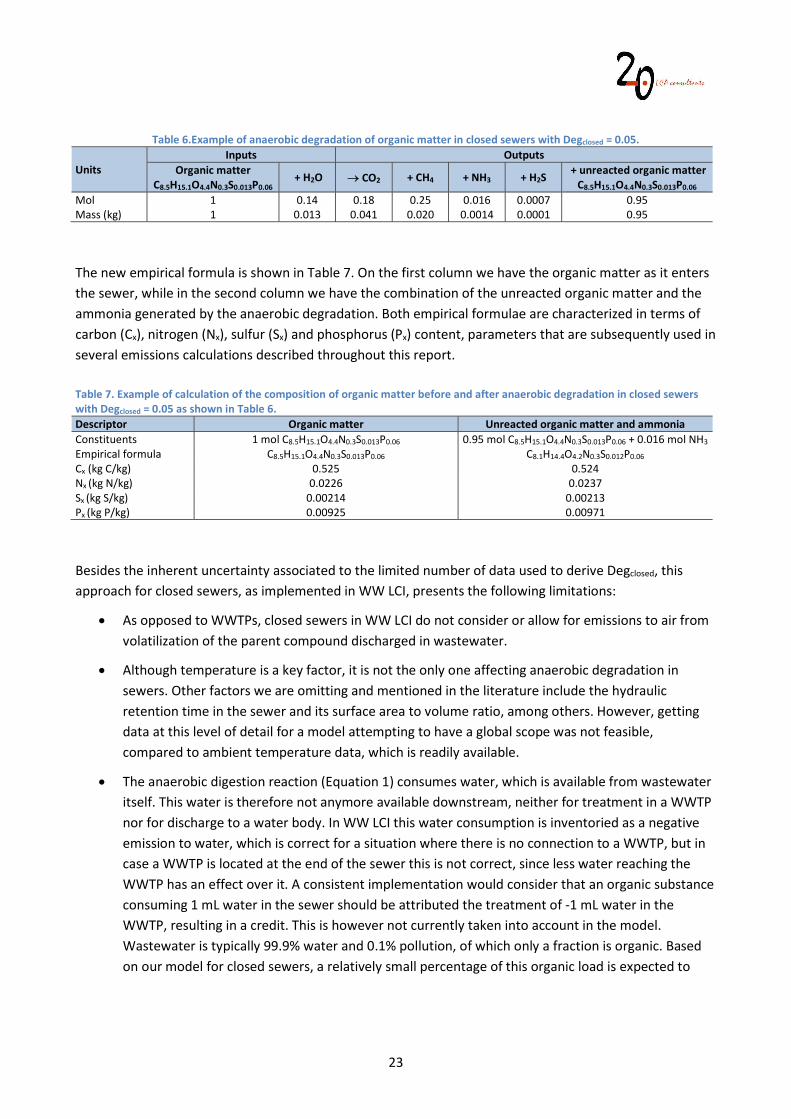
Table 6.Example of anaerobic degradation of organic matter in closed sewers with Degclosed = 0.05.

Units Inputs Outputs

Organic matter C8.5H15.1O4.4N0.3S0.013P0.06

+ H2O CO2 + CH4 + NH3 + H2S + unreacted organic matter

C8.5H15.1O4.4N0.3S0.013P0.06 Mol 1 0.14 0.18 0.25 0.016 0.0007 0.95 Mass (kg) 1 0.013 0.041 0.020 0.0014 0.0001 0.95 The new empirical formula is shown in Table 7. On the first column we have the organic matter as it enters the sewer, while in the second column we have the combination of the unreacted organic matter and the ammonia generated by the anaerobic degradation. Both empirical formulae are characterized in terms of carbon (Cx), nitrogen (Nx), sulfur (Sx) and phosphorus (Px) content, parameters that are subsequently used in several emissions calculations described throughout this report. Table 7. Example of calculation of the composition of organic matter before and after anaerobic degradation in closed sewers with Degclosed = 0.05 as shown in Table 6. Descriptor Organic matter Unreacted organic matter and ammonia Constituents 1 mol C8.5H15.1O4.4N0.3S0.013P0.06 0.95 mol C8.5H15.1O4.4N0.3S0.013P0.06 + 0.016 mol NH3 Empirical formula C8.5H15.1O4.4N0.3S0.013P0.06 C8.1H14.4O4.2N0.3S0.012P0.06 Cx (kg C/kg) 0.525 0.524 Nx (kg N/kg) 0.0226 0.0237 Sx (kg S/kg) 0.00214 0.00213 Px (kg P/kg) 0.00925 0.00971 Besides the inherent uncertainty associated to the limited number of data used to derive Degclosed, this approach for closed sewers, as implemented in WW LCI, presents the following limitations:

As opposed to WWTPs, closed sewers in WW LCI do not consider or allow for emissions to air from volatilization of the parent compound discharged in wastewater.

Although temperature is a key factor, it is not the only one affecting anaerobic degradation in sewers. Other factors we are omitting and mentioned in the literature include the hydraulic retention time in the sewer and its surface area to volume ratio, among others. However, getting data at this level of detail for a model attempting to have a global scope was not feasible, compared to ambient temperature data, which is readily available.

The anaerobic digestion reaction (Equation 1) consumes water, which is available from wastewater itself. This water is therefore not anymore available downstream, neither for treatment in a WWTP nor for discharge to a water body. In WW LCI this water consumption is inventoried as a negative emission to water, which is correct for a situation where there is no connection to a WWTP, but in case a WWTP is located at the end of the sewer this is not correct, since less water reaching the WWTP has an effect over it. A consistent implementation would consider that an organic substance consuming 1 mL water in the sewer should be attributed the treatment of -1 mL water in the WWTP, resulting in a credit. This is however not currently taken into account in the model. Wastewater is typically 99.9% water and 0.1% pollution, of which only a fraction is organic. Based on our model for closed sewers, a relatively small percentage of this organic load is expected to

24

degrade and consume water. Thus, the error induced by our simplification is expected to have a relatively low relevance in the LCI.

Another simplification made in the model is that, as seen in Figure 2, NH3 released by anaerobic degradation, expected to be in the form of ammonium, NH4

+, is not further modelled as ammonium, but rather integrated again with the remaining fraction of the parent compound, resulting in a new empirical formula for the material travelling downstream to the WWTP or to discharge. Again, this simplification is expected to incur in a very small difference as compared to modelling ammonium separately, but has the advantage of substantially reducing the number of calculations while still keeping the mass balance intact.

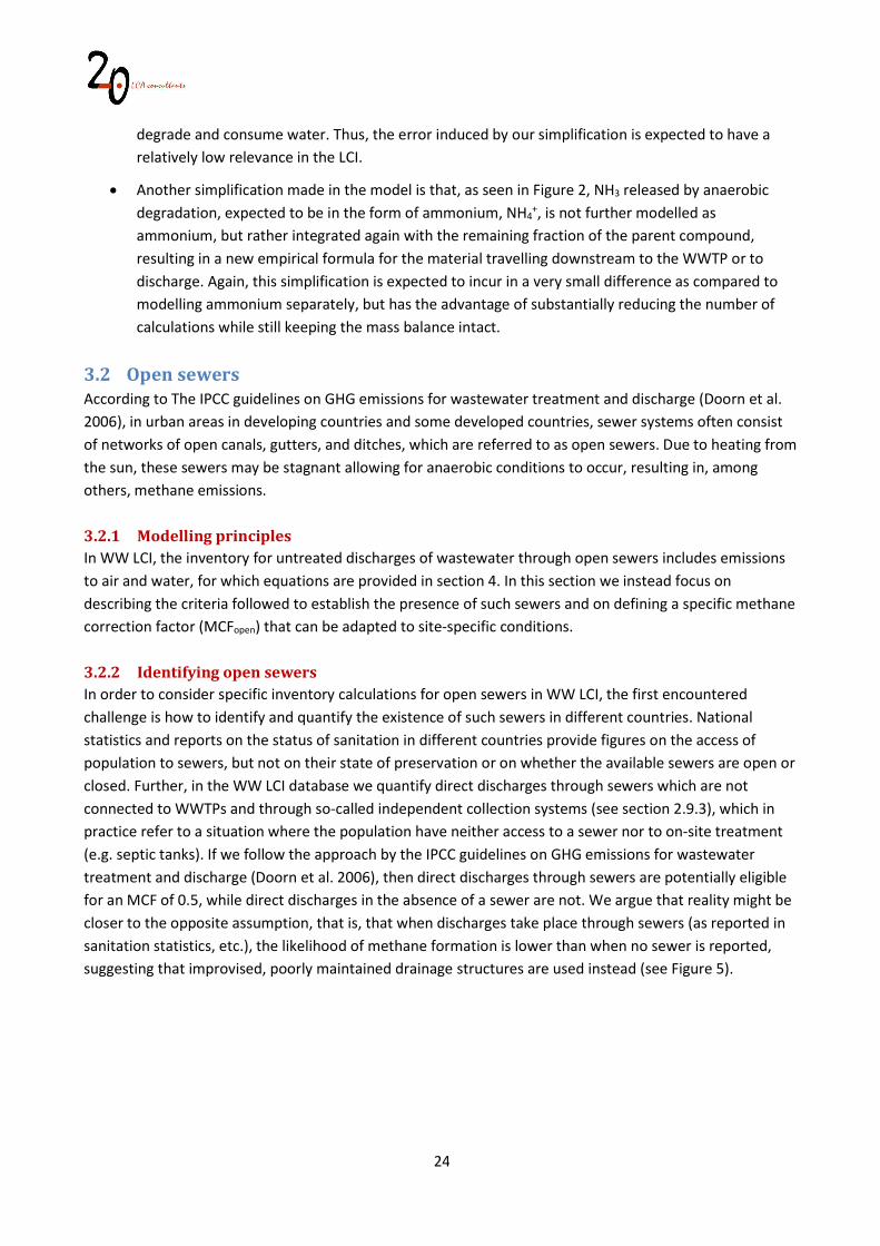
3.2 Open sewers According to The IPCC guidelines on GHG emissions for wastewater treatment and discharge (Doorn et al. 2006), in urban areas in developing countries and some developed countries, sewer systems often consist of networks of open canals, gutters, and ditches, which are referred to as open sewers. Due to heating from the sun, these sewers may be stagnant allowing for anaerobic conditions to occur, resulting in, among others, methane emissions. 3.2.1 Modelling principles In WW LCI, the inventory for untreated discharges of wastewater through open sewers includes emissions to air and water, for which equations are provided in section 4. In this section we instead focus on describing the criteria followed to establish the presence of such sewers and on defining a specific methane correction factor (MCFopen) that can be adapted to site-specific conditions. 3.2.2 Identifying open sewers In order to consider specific inventory calculations for open sewers in WW LCI, the first encountered challenge is how to identify and quantify the existence of such sewers in different countries. National statistics and reports on the status of sanitation in different countries provide figures on the access of population to sewers, but not on their state of preservation or on whether the available sewers are open or closed. Further, in the WW LCI database we quantify direct discharges through sewers which are not connected to WWTPs and through so-called independent collection systems (see section 2.9.3), which in practice refer to a situation where the population have neither access to a sewer nor to on-site treatment (e.g. septic tanks). If we follow the approach by the IPCC guidelines on GHG emissions for wastewater treatment and discharge (Doorn et al. 2006), then direct discharges through sewers are potentially eligible for an MCF of 0.5, while direct discharges in the absence of a sewer are not. We argue that reality might be closer to the opposite assumption, that is, that when discharges take place through sewers (as reported in sanitation statistics, etc.), the likelihood of methane formation is lower than when no sewer is reported, suggesting that improvised, poorly maintained drainage structures are used instead (see Figure 5).

25

Figure 5. Images of open sewers. Top left: Bangkok, Thailand; Top right: Bangalore, India; Bottom left: Kinshasa, Democratic Republic of Congo; Bottom-right: Ramadi, Iraq. All images from: https://www.crookedbrains.net/2008/01/open-sewers-of-world.html. Our interpretation is that access to sewers, as reported in country statistics, sanitation reports, etc., most likely corresponds to what the IPCC calls ‘Flowing sewer (open or closed)’, whereas it is the absence of a public sanitary sewer what most likely will lead to stagnant, anaerobic drainage. This, we think, is the most reasonable way to identify the presence of open sewers. In summary, we choose to consider the conditions of open, stagnant sewers when direct discharges take place in the absence of sewers, a situation which in WW LCI is classified as ‘Independent wastewater collecting systems - without treatment’. 3.2.3 Methane correction factor for open, stagnant sewers (MCFopen) The extent of anaerobic degradation in open, stagnant sewers is defined in WW LCI by a methane correction factor for open sewers (MCFopen), which expresses the extent of anaerobic (as opposed to

26

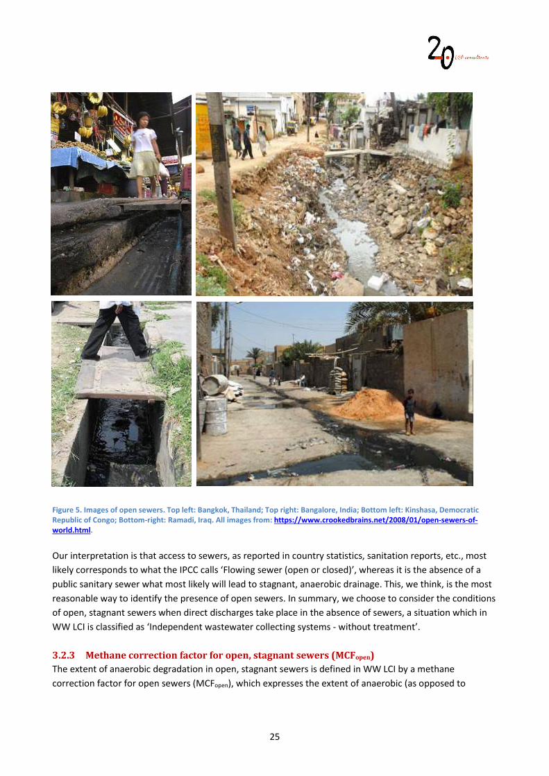
aerobic) degradation, for anaerobically degradable substances. The IPCC guidelines on GHG emissions for wastewater treatment and discharge (Doorn et al. 2006) propose a generic MCF value of 0.5, with a variability range between 0.4 and 0.8. In WW LCI we have attempted to go beyond this approach since the extent of anaerobic conditions in sewers varies according to several variables, most notably climate. In fact, we contacted Michiel Doorn (lead author of the IPCC report on wastewater treatment and discharge, Doorn et al. 2006) to discuss this issue. To the question of whether or not climate is an important variable, for example to differentiate methane emissions in countries like Russia and India, Mr. Doorn kindly replied, stating: “You are right that a hot climate would enhance rapid anaerobic conditions to manifest, as would stagnant water” and also “I agree with you that Russia would be very different than India for reasons of climate and perhaps infrastructure. Basically, the MCF was an educated guess” (Doorn 2018). We decided to incorporate climatic conditions as part of the determination of the MCFopen, in a similar way as we do for closed sewers. In this case, however, we did not find specific models for emissions occurring in these types of systems. For this reason, we decided to use the IPCC’s proposed MCF as a starting point and adjust it according to ambient temperature. For this purpose, we used the sewer model by Chaosakul et al. (2014), in which the effect of temperature is taken into account by the coefficient 1.05 (T – 20), where T is the wastewater temperature (ºC). The MCF proposed by the IPCC ranges between 0.4 and 0.8; we take a value of 0.75 as a worst case (Doorn and Liles 1999). This worst-case value is used only for the country with the highest mean annual air temperature, which according to Weatherbase (2020), is Mali (28.2 ºC). We calculate MCFopen with Equation 4:

MCFopen = 0.75 1.05 (Ta – 20)

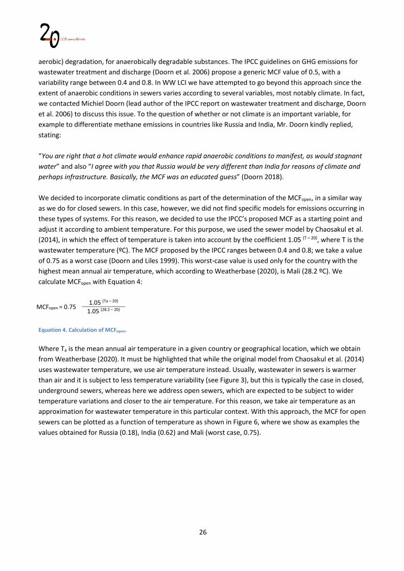
1.05 (28.2 – 20) Equation 4. Calculation of MCFopen. Where Ta is the mean annual air temperature in a given country or geographical location, which we obtain from Weatherbase (2020). It must be highlighted that while the original model from Chaosakul et al. (2014) uses wastewater temperature, we use air temperature instead. Usually, wastewater in sewers is warmer than air and it is subject to less temperature variability (see Figure 3), but this is typically the case in closed, underground sewers, whereas here we address open sewers, which are expected to be subject to wider temperature variations and closer to the air temperature. For this reason, we take air temperature as an approximation for wastewater temperature in this particular context. With this approach, the MCF for open sewers can be plotted as a function of temperature as shown in Figure 6, where we show as examples the values obtained for Russia (0.18), India (0.62) and Mali (worst case, 0.75).

27

Figure 6. MCFopen as a function of mean annual temperature, as implemented in WW LCI.

3.3 WWTP with secondary treatment – activated sludge Centralized treatment in a WWTP using activated sludge constitutes one of the pillars of WW LCI, as this was the only type of plant included in the model’s first version. Subsequent wastewater treatment options added to the model up to date rely on the framework developed for this type of plant. 3.3.1 Modelling principles The WWTP model includes a primary settling tank, an activated sludge biological treatment, a secondary settling tank, and sludge treatment consisting of at least gravity thickening and dewatering. The model also considers optional anaerobic digestion of combined primary and secondary sludge, which is included or excluded depending on the scenario data. This type of plant does not include dedicated nutrient removal. Thus, nitrogen is only removed from wastewater by settling, incorporation in sludge biomass and through fugitive N2O emissions. Similarly, phosphorus is only removed by settling and incorporation in sludge biomass. The inventory for this WWTP includes the following aspects:

WWTP infrastructure (section 3.3.2). Electricity balance (section 6.1). Thermal energy (natural gas and biogas) balance (section 6.2). Chemical reagents (polyelectrolyte for sludge conditioning, see section 5.1.4). Emissions to air and water resulting from the treated effluent (section 4). Emissions to air from the WWTP basins (sections 3.3.4 and 3.3.6). Emissions to air from combustion of biogas, if applicable (section 5.1.2). Substituted nutrient treatment due to nutrient consumption (section 3.3.7)

0.0

0.1

0.2

0.3

0.4

0.5

0.6

0.7

0.8

-5 0 5 10 15 20 25 30

MCF

in

open

sew

ers

Mean annual air temperature (ºC)

Mali

· India

·

· Russia

28

3.3.2 WWTP infrastructure Inputs of WWTP infrastructure are attributed equally to all substances treated in an activated sludge plant, on a mass basis. In this way, 1 kg water, 1 kg COD or 1 kg surfactant all receive the same inputs of WWTP infrastructure. This activity is modelled with the ecoinvent data sets for WWTP, which include five capacity classes. As in the ecoinvent database, the size of the sewer is linked to the size of the WWTP connected to it. In WW LCI, ecoinvent data sets are associated to the following plant capacities, on a daily flow basis:

Data set for a flow of 4.7E+10 L/year used for WWTPs treating ≥55,000 m3/d. Data set for a flow of 1.1E+10 L/year used for WWTPs treating between 28,000 m3/d and 54,999

m3/d. Data set for a flow of 5E+09 L/year used for WWTPs treating between 5,500 m3/d and 27,999 m3/d. Data set for a flow of 1E+09 L/year used for WWTPs treating between 1,100 m3/d and 5,499 m3/d. Data set for a flow of 1.6E+08 L/year used for WWTPs treating <1,100 m3/d.

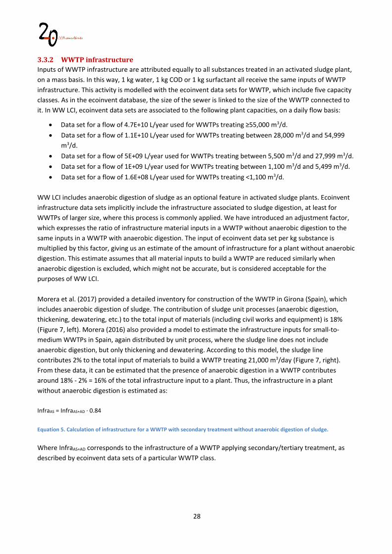
WW LCI includes anaerobic digestion of sludge as an optional feature in activated sludge plants. Ecoinvent infrastructure data sets implicitly include the infrastructure associated to sludge digestion, at least for WWTPs of larger size, where this process is commonly applied. We have introduced an adjustment factor, which expresses the ratio of infrastructure material inputs in a WWTP without anaerobic digestion to the same inputs in a WWTP with anaerobic digestion. The input of ecoinvent data set per kg substance is multiplied by this factor, giving us an estimate of the amount of infrastructure for a plant without anaerobic digestion. This estimate assumes that all material inputs to build a WWTP are reduced similarly when anaerobic digestion is excluded, which might not be accurate, but is considered acceptable for the purposes of WW LCI. Morera et al. (2017) provided a detailed inventory for construction of the WWTP in Girona (Spain), which includes anaerobic digestion of sludge. The contribution of sludge unit processes (anaerobic digestion, thickening, dewatering, etc.) to the total input of materials (including civil works and equipment) is 18% (Figure 7, left). Morera (2016) also provided a model to estimate the infrastructure inputs for small-to-medium WWTPs in Spain, again distributed by unit process, where the sludge line does not include anaerobic digestion, but only thickening and dewatering. According to this model, the sludge line contributes 2% to the total input of materials to build a WWTP treating 21,000 m3/day (Figure 7, right). From these data, it can be estimated that the presence of anaerobic digestion in a WWTP contributes around 18% - 2% = 16% of the total infrastructure input to a plant. Thus, the infrastructure in a plant without anaerobic digestion is estimated as: InfraAS = InfraAS+AD · 0.84 Equation 5. Calculation of infrastructure for a WWTP with secondary treatment without anaerobic digestion of sludge. Where InfraAS+AD corresponds to the infrastructure of a WWTP applying secondary/tertiary treatment, as described by ecoinvent data sets of a particular WWTP class.

29

12%

10%

54%

18%

6%

Pumping and pre-treatment

Primary treatment

Secondary treatment

Sludge treatment

Other

2%

22%

2%

1%

2%

50%

Pretreatment

Secondary treatment

Sludge treatment

Tube connections

Buildings

Urbanization

Figure 7. Relative distribution of infrastructure materials in a WWTP with secondary/tertiary treatment. Left: WWTP in Girona, Spain, treating 42,000 m3/day and including anaerobic digestion of sludge. Right: Hypothetical WWTP in Spain, treating 21,000 m3/day, without anaerobic digestion of sludge. Based on data from Morera et al. (2017) and Morera (2016). Table 8 shows the infrastructure inputs attributed to 1 kg wastewater component. The first column shows the values used in the ecoinvent database, per L wastewater, while the second column shows the values after applying Equation 5. As it can be seen, this parameter does not affect the smallest WWTP class, as we assume the application of anaerobic digestion of sludge is unlikely in this case.

Table 8. Infrastructure inputs per kg substance in a WWTP with secondary treatment by activated sludge.

Activity WWTP with

anaerobic digestion

WWTP without anaerobic digestion

WWTP infrastructure input for WWTPs > 55,000 m3/d (unit/kg) 6.06E-13 5.09E-10 WWTP infrastructure input for WWTPs 28,000-55,000 m3/d (unit/kg) 1.99E-12 1.67E-09 WWTP infrastructure input for WWTPs 5,500-28,000 m3/d (unit/kg) 5.69E-12 4.78E-09 WWTP infrastructure input for WWTPs 1,100-5,500 m3/d (unit/kg) 2.66E-11 2.23E-11 WWTP infrastructure input for WWTPs <1,100 m3/d (unit/kg) 1.75E-10 1.75E-10 For all countries in the WW LCI database a WWTP capacity mix is provided, which states the percentage of wastewater treated under each one of the five WWTP classes. This information is combined with the percentage of wastewater treated in WWTPs with anaerobic digestion, also stored in the database, in order to apply one of the two values shown in Table 8 for each WWTP class. 3.3.3 Fate factors Figure 8 provides an overview of how the mass balance in the WWTP is addressed by the model. Substance-specific fate factors Fa, Fdeg, Fsludge and Feffluent are used to describe to what extent a given chemical substance is subject to different phenomena. The fate factors Fair and Feffluent determine the fraction of 1 kg substance entering the WWTP that is released to air or in the treated effluent. The fate factor Fdeg determines the fraction expected to be degraded biologically in the aeration basin. Degradation products include emissions to air, such as CO2 and emissions to water in the treated effluent, such as ammonium or phosphate. Degradation is carried out by microorganisms in the aeration basin, which use the substance as a substrate for growth. This leads to excess activated sludge. Finally, Fsludge determines the fraction partitioned to sludge as a result of primary and secondary settling. Excess activated sludge and Fsludge can be either directly sent for disposal, or treated

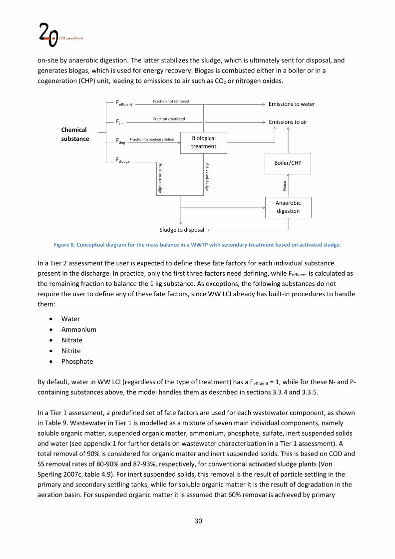
30

on-site by anaerobic digestion. The latter stabilizes the sludge, which is ultimately sent for disposal, and generates biogas, which is used for energy recovery. Biogas is combusted either in a boiler or in a cogeneration (CHP) unit, leading to emissions to air such as CO2 or nitrogen oxides.

Figure 8. Conceptual diagram for the mass balance in a WWTP with secondary treatment based on activated sludge.

In a Tier 2 assessment the user is expected to define these fate factors for each individual substance present in the discharge. In practice, only the first three factors need defining, while Feffluent is calculated as the remaining fraction to balance the 1 kg substance. As exceptions, the following substances do not require the user to define any of these fate factors, since WW LCI already has built-in procedures to handle them:

Water Ammonium Nitrate Nitrite Phosphate

By default, water in WW LCI (regardless of the type of treatment) has a Feffluent = 1, while for these N- and P-containing substances above, the model handles them as described in sections 3.3.4 and 3.3.5. In a Tier 1 assessment, a predefined set of fate factors are used for each wastewater component, as shown in Table 9. Wastewater in Tier 1 is modelled as a mixture of seven main individual components, namely soluble organic matter, suspended organic matter, ammonium, phosphate, sulfate, inert suspended solids and water (see appendix 1 for further details on wastewater characterization in a Tier 1 assessment). A total removal of 90% is considered for organic matter and inert suspended solids. This is based on COD and SS removal rates of 80-90% and 87-93%, respectively, for conventional activated sludge plants (Von Sperling 2007c, table 4.9). For inert suspended solids, this removal is the result of particle settling in the primary and secondary settling tanks, while for soluble organic matter it is the result of degradation in the aeration basin. For suspended organic matter it is assumed that 60% removal is achieved by primary

Chemical substance

Feffluent

Fair

Fdeg

Fsludge

Emissions to air

Biologicaltreatment

Sludge to disposal

Emissions to waterFraction not removed

Fraction volatilized

Fraction to biodegradation

Fractionto sludge

Activated

sludge

Biog

as

Boiler/CHP

Anaerobicdigestion

31

settling, based on a typical removal of suspended solids ranging from 55%-65% for conventional primary treatment (Von Sperling 2007c, table 4.9), while the remaining 30% removal is assumed to be achieved by degradation in the aeration basin. Water, ammonium and phosphate, though, do not require the definition of fate factors, as discussed in the previous paragraph. The fate of metals in the WWTP is based on data from Yoshida et al (2015), except for Arsenic, which is based on Cecchinit al. (2015).

Table 9. Fate factors for wastewater components in a Tier 1 assessment of a WWTP with secondary treatment by activated sludge. Not applicable: n.a.

Activity Fair Fdeg Fsludge Soluble organic matter 0 0.9 0 Suspended organic matter 0 0.3 0.6 Inert suspended solids 0 0 0.9 Ammonium n.a. n.a. n.a. Phosphate n.a. n.a. n.a. Sulfate n.a. n.a. n.a. Water n.a. n.a. n.a. Silver n.a. n.a. 0.74 Aluminium n.a. n.a. 0.96 Arsenic n.a. n.a. 0.27 Cadmium n.a. n.a. 0.86 Chromium n.a. n.a. 0.87 Copper n.a. n.a. 0.98 Mercury n.a. n.a. 0.90 Manganese n.a. n.a. 0.47 Nickel n.a. n.a. 0.46 Lead n.a. n.a. 0.96 Zinc n.a. n.a. 0.91 Barium n.a. n.a. 0.86 Cobalt n.a. n.a. 0.72 Iron n.a. n.a. 0.83 Magnesium n.a. n.a. 0.05 Antimony n.a. n.a. 0.54 Vanadium n.a. n.a. 0.83

3.3.4 Biological treatment: carbonaceous organic matter removal The fraction of chemical undergoing degradation (Fdeg) is subject to a series of biochemical reactions in the WWTP’s aeration basin, where a fraction of the carbon contained in the chemical substrate is oxidized by aerobic microorganisms (biomass) to CO2, while the rest is incorporated into new biomass. This conversion is included by means of Equation 6: CaHbOcNd + A O2 B C5H7O2N + C CO2 + D H2O + E NH4 A = 1/2 · (2B + 2C + D - c) B = 1/5 · (a - C) C = (1 - Yobs ) · a D = 1/2 · (b - 7B - 4E) E = d - B Equation 6. Chemical equation for carbonaceous organic matter removal in biological treatment and calculation of stoichiometric coefficients.

32

Where CaHbOcNd is the empirical formula for the assessed substance. Elements other than carbon, hydrogen, oxygen and nitrogen are not taken into account in this calculation, but considered in the overall mass balance. A possible situation is that the assessed substance does not contain nitrogen, or contains less than necessary to fulfill the requirements of sludge biomass growth, represented by the formula C5H7O2N. In this case, the sign of stoichiometric coefficient E becomes negative, meaning that the reaction consumes rather than produces ammonium, and this ammonium is obtained from the surrounding wastewater. Modelling of such nutrient consumption is described in section 3.3.7. Production of excess biomass sludge in Equation 6 takes into account the observed yield, Yobs, calculated with Equation 7:

Yobs = 1.42 · Y

1 + kd · c Equation 7. Calculation of the observed biomass yield in biological treatment. Where:

Yobs is the observed yield or net amount of biomass produced per unit of mass substrate removed, expressed as g COD in biomass/g COD removed.

Y is the yield or amount of biomass produced per unit of mass substrate removed, expressed in g VSS/g COD removed. This parameter ranges from 0.3 to 0.7 (von Sperling 2007a, p. 94). A value of 0.5 is used in WW LCI.

1.42 is the COD of VSS assuming the empirical formula C5H7O2N (Von Sperling 2007b, p. 28).

kd is the endogenous respiration coefficient or bacterial decay coefficient (day-1), ranging from 0.05 to 0.12 (von Sperling 2007a, p. 92). A value of 0.085 is used in WW LCI.

c is the sludge residence time (SRT) in the system, in days. Values for activated sludge systems range from 4 to 10 days, although in extended aeration systems it can be as long as 30 days (Von Sperling 2007c). In WW LCI we model an activated sludge treatment plant without nutrient removal, therefore a relatively short SRT can be considered. A value of 5 days is chosen as a default.

It must be highlighted that all values for parameters in Equation 7 can be modified by the user. 3.3.5 Biological treatment: fate of phosphorus, sulfur and chlorine This section describes the fate of phosphorus (P), sulfur (S) and chlorine (Cl) contained in the fraction Fdeg, i.e. the fraction of substance subject to biodegradation as described in Equation 6, which does not capture these elements. Some P is taken up by new biomass formed in the biological reactor. Although in Equation 6 biomass is represented with the formula C5H7O2N, a separate calculation in the model accounts for this, with a factor of 0.02 kg P removed per kg biomass, based on the empirical formula C5H7O2NP0.074 (Droste et al. 1997). When the degraded substance contains more P than necessary for biomass growth, this is assumed in the

33

model to be in the form of orthophosphate (PO4), which is released in the effluent. The amount of oxygen needed to form PO4 is stoichiometrically calculated as 2.065 kg O/kg P. This oxygen contributes to the electricity demand for aeration (see section 6.1). As mentioned for nitrogen in the previous section, there can be a situation where a substance degrades but it does not contain P. In this case, the required amount of P is taken from the surrounding wastewater. The modelling of this nutrient consumption is discussed in section 3.3.7. Any S or Cl required for biomass growth is neglected by the model. Thus, S arising from degradation of chemicals is assumed to be fully converted to sulfate (SO4) and discharged with the treated effluent. The stoichiometric mass of oxygen needed for this oxidation is taken into account in the mass balance (2 kg O/kg S), and this oxygen contributes to the electricity demand for aeration (see section 6.1). As for Cl, it is assumed to be fully released as chloride in the treated effluent. 3.3.6 Biological treatment: N2O emissions Part of the N input undergoing degradation in the WWTP is considered to be released as dinitrogen monoxide (N2O). As shown by several studies, N2O emissions are extremely variable (Kampschreur et al. 2009; Law et al. 2012; Ahn et al. 2010) as well as highly relevant in the life cycle greenhouse-gas (GHG) emissions of WWTPs (Foley et al. 2010; Chai et al. 2015). In WW LCI N2O emissions are only calculated for substances that undergo degradation, i.e. having a fate factor Fdeg > 0 and that contain excess nitrogen. By excess nitrogen we refer to substances where coefficient E in Equation 6 has a positive sign, meaning that degradation results in the formation of ammonium. Conversely, if a nitrogen-containing substance degrades and coefficient E is zero or negative, no N2O emissions are calculated. N2O emissions are quantified based on a generic emission factor, set at 0.005 kg N2O-N/kg NH4-N released in Equation 6. This value is within the range of previously used values by two LCI models, namely ORWARE (0.0015) and ecoinvent (0.0068) (Dalemo 1997; Doka 2007). As for most other parameters in WW LCI, this default value can be modified by the user. 3.3.7 Biological treatment: nutrient consumption As mentioned in sections 3.3.4 and 3.3.5 there are situations in which a substance is degraded by the microorganisms in the aeration basin, but it does not contain enough P and/or N to fulfil the nutrient requirements by microoorganisms. We illustrate how this type of situation is handled in WW LCI with the chemical ethanol, as done in Muñoz (2017). Once in a WWTP with secondary treatment, ethanol is expected to be degraded by microorganisms that have certain requirements for nutrients such as nitrogen and phosphorus. In WW LCI, biomass formed by biological treatment is characterized with the formula C5H7NO2P0.074 (see section 3.3.5), which means every time 5 mol organic carbon is taken in to build biomass, 1 mol N and 0.074 mol P are needed. In the case of ethanol (C2H6O) this cannot be supplied by the compound itself. In industrial WWTPs this problem is overcome by adding nutrients from external sources, such as urea or phosphoric acid. In urban WWTPs, though, there is no need for this, as these nutrients can be supplied by other wastewater streams with an excess of N and P and which end up in the same WWTP as ethanol. These nutrients in urban wastewater are an example of ‘not fully utilized’ materials (Consequential LCA 2015), whereby additional demand for

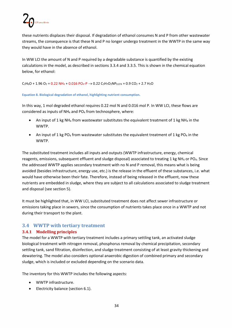
34

these nutrients displaces their disposal. If degradation of ethanol consumes N and P from other wastewater streams, the consequence is that these N and P no longer undergo treatment in the WWTP in the same way they would have in the absence of ethanol. In WW LCI the amount of N and P required by a degradable substance is quantified by the existing calculations in the model, as described in sections 3.3.4 and 3.3.5. This is shown in the chemical equation below, for ethanol: C2H6O + 1.96 O2 + 0.22 NH4 + 0.016 PO4-P 0.22 C5H7O2NP0.074 + 0.9 CO2 + 2.7 H2O Equation 8. Biological degradation of ethanol, highlighting nutrient consumption. In this way, 1 mol degraded ethanol requires 0.22 mol N and 0.016 mol P. In WW LCI, these flows are considered as inputs of NH4 and PO4 from technosphere, where:

An input of 1 kg NH4 from wastewater substitutes the equivalent treatment of 1 kg NH4 in the WWTP.

An input of 1 kg PO4 from wastewater substitutes the equivalent treatment of 1 kg PO4 in the WWTP.

The substituted treatment includes all inputs and outputs (WWTP infrastructure, energy, chemical reagents, emissions, subsequent effluent and sludge disposal) associated to treating 1 kg NH4 or PO4. Since the addressed WWTP applies secondary treatment with no N and P removal, this means what is being avoided (besides infrastructure, energy use, etc.) is the release in the effluent of these substances, i.e. what would have otherwise been their fate. Therefore, instead of being released in the effluent, now these nutrients are embedded in sludge, where they are subject to all calculations associated to sludge treatment and disposal (see section 5). It must be highlighted that, in WW LCI, substituted treatment does not affect sewer infrastructure or emissions taking place in sewers, since the consumption of nutrients takes place once in a WWTP and not during their transport to the plant.

3.4 WWTP with tertiary treatment 3.4.1 Modelling principles The model for a WWTP with tertiary treatment includes a primary settling tank, an activated sludge biological treatment with nitrogen removal, phosphorus removal by chemical precipitation, secondary settling tank, sand filtration, disinfection, and sludge treatment consisting of at least gravity thickening and dewatering. The model also considers optional anaerobic digestion of combined primary and secondary sludge, which is included or excluded depending on the scenario data. The inventory for this WWTP includes the following aspects:

WWTP infrastructure. Electricity balance (section 6.1).

35

Thermal energy (natural gas and biogas) balance (section 6.2). Chemical reagents and auxiliary materials: polyelectrolyte for sludge conditioning (section 5.1.4),

sodium hypochlorite for disinfection (section 3.4.7), ferric chloride for phosphorus removal (section 3.4.5), sodium hydroxide and sand for sand filter (section 3.4.6).

Emissions to air and water resulting from the treated effluent (section 4). Emissions to air from the WWTP basins (sections 3.4.2 and 3.4.3). Emissions to air from combustion of biogas, if applicable (section 5.1.2). Substituted nutrient treatment due to nutrient consumption (section 3.3.7)

Several aspects described in section 3.3 for WWTPs with secondary treatment applying activated sludge are equivalent in WW LCI to model WWTPs with tertiary treatment, and they are therefore not further addressed. These include:

WWTP infrastructure: the description in section 3.3.2 applies.

Fate factors: the description in section 3.3.3 applies, supplemented by the additional considerations for sand filtration (see section 3.4.6).

Biological treatment: the descriptions in section 3.3.5 on the fate of sulfur and chlorine apply, while fate of phosphorus is subject to changes described in section 3.4.5, to account for phosphorus removal. The quantification of N2O emissions in section 3.3.6 also applies, while some additional comments are given on nutrient consumption in section 3.4.4.

3.4.2 Biological treatment: carbonaceous organic matter removal Degradation of organic matter in a WWTP with tertiary treatment relies on the same calculations described in section 3.3.4, i.e. the substance-specific fate factor Fdeg is used to quantify the extent of degradation, while Equation 6 is used to represent the biochemical process. The only difference is the calculation of Yobs with Equation 7, where a different value for sludge residence time, c, is used. The reason is that the WWTP applies N removal, consisting of a nitrification-denitrification process (described in the next section). Achieving complete nitrification typically requires long sludge residence times, given that the reproduction rate of nitrifying organisms is much smaller than that of the heterotrophic organisms responsible for the stabilization of carbonaceous organic matter. According to Von Sperling (2007b), the total sludge residence time in systems applying either pre-denitrification or post-denitrification range between 6 to 10 days, while for extended aeration systems it ranges between 10 to 30 days. However, in order to model carbonaceous organic matter removal, we are interested in the aerobic sludge residence time, that is, the fraction of the total sludge residence time under aerobic conditions. According to the same source, this is a minimum of 5 days for pre-denitrification and post-denitrification systems and a minimum of 8 days for extended aeration systems. In WW LCI a value of 9 days is used. This is the average for different N removal configurations assessed by Foley et al. (2010), ranging from 7.5 to 10 days for a modified Ludzack-Ettinger process and 9 to 11.25 days for a Bardenpho process. 3.4.3 Biological treatment: nitrogen removal Nitrogen removal in WW LCI is modelled as a nitrification-denitrification, process, however no particular configuration is addressed. This process applies only to degradable organic substances that produce

36

ammonium as a result of carbonaceous organic matter removal. It also applies to the hypothetical case where the user, in a Tier 2 assessment, declares ammonium or nitrate as part of the wastewater mixture. The nitrification reaction is included in WW LCI by means of Equation 9: NH4

+ + 1.855 O2 + 2 HCO3- 0.02 C5H7ON2 + 0.98 NO3

- + 1.03 H2O + 1.9 H2CO3

Equation 9. Chemical equation for nitrification. Equation 9 is derived from Qasim (1999), with small modifications in the stoichiometric coefficients to ensure a mass balance when the following atomic weights are used, in g/mol: C = 12, H = 1, O = 16 and N =14. Nitrification consumes alkalinity, expressed in Equation 9 as bicarbonate (HCO3

-) and this might lead to a reduction in the pH, which affects the nitrification rate. Depending on the alkalinity available in wastewater, this imbalance needs to be addressed by the addition of a pH-correcting agent, such as lime. In WW LCI this is not included. The main reason is that alkalinity consumption by nitrification is partly compensated by consumption of H+ ions in the denitrification reaction (see Equation 10 and Equation 11). Under these conditions, it is assumed that addition of an external source of alkalinity is not needed. Biological denitrification requires the presence in wastewater of an organic carbon source acting as electron donor, which can be added artificially or be available internally in wastewater. In WW LCI the former option is modelled with the addition of methanol as shown in Equation 10: NO3

- + 1.08 CH3OH + 0.9 H+ 0.06 C5H7ON2 + 0.47 N2 + 0.78 CO2 + 2.4 H2O

Equation 10. Chemical equation for denitrification using methanol as organic carbon source. Equation 10 is derived from Qasim (1999), with small modifications in the stoichiometric coefficients as mentioned for nitrification. Methanol is considered as an external input in the inventory and the carbon embedded in the product is assumed to originate in fossil sources. Thus, the carbon embedded in the CO2

and biomass (C5H7ON2) obtained as a result of this process is also labelled as fossil. As a default, though, WW LCI does not use Equation 10 unless the user deliberately chooses this option. This is based on the assumption that N removal systems requiring the addition of methanol are less common than those using organic carbon already present in wastewater. We have found little data to back this up quantitatively, let alone to specify it as a country-specific variable in the WW LCI database. The methanol Institute (2018) claims that there are nearly 200 WWTPs in the United States using methanol. The total number of urban WWTPs with advanced treatment, according to the Clean Watersheds Needs Survey in 2012 (USEPA 2018) is 4,971. Assuming that this is the number of plants applying N removal in the United States, only about 4% of the operating plants apply N removal with methanol. The default denitrification process in WW LCI considers the use of organic carbon already present in wastewater. This is modelled as a simplified version of the above reaction, as shown in Equation 11:

37

NO3- + 6 H+ 0.5 N2 + 3 H2O

Equation 11. Chemical equation for denitrification without the addition of methanol as organic carbon source. This simplified chemical equation still keeps stoichiometry and implies that denitrification results in no consumption of methanol, but also in no production of excess biomass sludge or CO2. This simplification leads to an underestimation of the amount of excess sludge and CO2 produced by the WWTP, however the contribution of this process to the overall sludge and CO2 production by biological treatment is minor, when compared to that by carbonaceous organic matter removal. Finally, the extent of nitrification and denitrification in the WWTP is defined with the following default factors, estimated based on figure 3.4 in Von Sperling (2007a):

For nitrification, ammonium-N conversion in Equation 9 is set to 90%. The remaining 10% is found in the treated effluent.

For denitrification, nitrate-N conversion in Equation 10 and Equation 11 is set to 80%, while the remaining 20% nitrate-N is found in the treated effluent.

3.4.4 Biological treatment: nutrient consumption Nutrient consumption in WWTPs with tertiary treatment is modelled under the same principles described for WWTPs with secondary treatment in section 3.3.7. However, in a WWTP with tertiary treatment there is dedicated N and P removal. This means that, as opposed to a WWTP with secondary treatment, in a WWTP with tertiary treatment:

NH4 consumption substitutes its removal in the WWTP by means of nitrification-denitrification, as described in section 3.4.3, instead of its release in the effluent.

PO4 consumption substitutes its removal in the WWTP by means of chemical precipitation, as described in section 3.4.5, instead of its release in the effluent.

3.4.5 Phosphorus removal In WW LCI, P removal is only considered for substances fulfilling the following conditions:

They must contain P.

Only P in the degraded fraction (Fdeg) is considered to be available for removal. This P is assumed, as described in section 3.3.5, to be available as orthophosphate.

The amount of P available for removal in Fdeg excludes the amount required for biomass growth, as described in section 3.3.5.

Enhanced P removal in WW LCI is considered by means of chemical precipitation, but no specific configuration is addressed (pre-precipitation in raw wastewater, simultaneous precipitation in the aeration tank, post-precipitation after secondary settling). Although this precipitation can be carried out with various chemicals, only ferric chloride is considered in the model. Ferric chloride is among the most widely used chemicals for this purpose (Paul et al. 2001). The chemical precipitation reaction is shown in Equation 12:

38

PO43- + A FeCl3 + B OH- FePO4 + C Fe(OH)3 + D Cl-

B = 3C - 3 C = A – 1 D = 3A Equation 12. Chemical equation for phosphorus removal by chemical precipitation and calculation of stoichiometric coefficients. Orthophosphate is precipitated as iron phosphate, which is settled with sludge. In Equation 12 the stoichiometry coefficients B, C and D are dependent on coefficient A, which can be defined as the chemical coagulant efficiency (mol FeCl3 applied/mol FeCl3 theoretically required). This coefficient must be ≥1. When it takes a value above 1 it means the chemical coagulant is applied in excess and part of the iron ions are precipitated as iron hydroxide, which is also settled in sludge. As a default, in WW LCI a value of 1.5 is used for the A coefficient, based on Paul et al. (2001). Based on this same reference, a default removal level of 80% of the available orthophosphate is considered. The remaining 20% is found in the treated effluent, as are the chloride ions released by the coagulant. As with most other parameters in WW LCI, this P removal level, as well as the value of the A coefficient can be modified by the user. 3.4.6 Sand filtration As part of tertiary treatment, WW LCI considers rapid sand filtration of the effluent from secondary treatment, aiming to capture small particles of suspended solids. The inventory for operation of the sand filter includes inputs of sodium hydroxide for cleaning, periodic replacement of sand, and energy consumption. Use of sodium hydroxide and sand is estimated at 7.46 g/m3 and 16.14 g/m3, respectively (Muñoz et al. 2010), while energy use for this unit process is addressed as part of section 6.1.2. On the one hand, these material and energy inputs are attributed equally to all substances passing through the filter, on a mass basis. In this way, 1 kg water, 1 kg COD or 1 kg surfactant all receive the same inputs. On the other hand, the effectiveness of the sand filter in removing pollutants is evaluated on a substance-specific basis, following the approach by Kalbar et al. (2017), as described below. The fraction of a substance adsorbed to the suspended solid phase in the secondary effluent is estimated according to Stuer-Lauridsen et al. (2000), as shown in Equation 13: Kd = foc · 0.41 · Kow

Equation 13. Calculation of the solid/liquid partition coefficient in suspended solids for sand filtration. Where Kd is the solid/liquid partition coefficients in suspended solids (dimensionless), foc is the fraction of organic carbon in the secondary effluent’s suspended solids (dimensionless), taken as 0.35 (Stuer-Lauridsen et al. 2000) and Kow is the octanol-water partitioning coefficient for the specific substance (dimensionless). In case of dissociating compounds, i.e. acids and bases according to the Brønsted–Lowry acid–base definition, Dow is used instead of Kow:

39

Kd = foc · 0.41 · Dow

Equation 14. Calculation of the solid/liquid partition coefficient in suspended solids for sand filtration in the case of dissociating compounds. Where Dow is the pH-corrected octanol-water partitioning coefficient of an organic compound, accounting for the pH dependency of Kow induced by the presence of ionisable groups in an organic molecule (dimensionless). Dow can be estimated as:

Dow = Kow

1 + 10 (pH -pKa) Equation 15. Calculation of pH-corrected octanol-water partitioning coefficient for dissociating compounds. Where pH is the pH of the effluent, taken as 6.5 (Metcalf et al. 2007) and pKa is the acid dissociation constant of the assessed compound, both dimensionless. The fraction of compound adsorbed to the suspended solids in the secondary effluent is calculated using the following equation (Andersen et al. 2004):

Fsorb = ρsludge · Kd

1 + ρsludge · Kd Equation 16. Calculation of the fraction of compound adsorbed to suspended solids in the secondary effluent. Where ρsludge is the density of suspended solids in the secondary effluent, in g/L, taken as 721 (Andersen et al. 2004). The substance-specific fate factor in the sand filter is finally calculated with Equation 17: Fsludge-sand = (1 - Fair - Fdeg -Fsludge) · Fsorb · Fsand Equation 17. Calculation of the fate factor in the sand filter. Where Fsludge-sand is the fraction of compound entering the WWTP that is expected to be removed in the sand filter and Fsand is the expected removal rate for suspended solids in the sand filter, taken as 71% from Benth et al. (1981). Fsludge-sand represents the additional pollution removal rate in a WWTP with a sand filter, which is not captured by the generic sludge fate factor Fsludge, the latter reflecting only the fraction removed by primary and secondary settling. Thus, in WW LCI the total partitioning to sludge of a given substance in a WWTP with tertiary treatment is reflected by the sum of Fsludge-sand and Fsludge. 3.4.7 Disinfection Disinfection in WW LCI is included as dosing of sodium hypochlorite (NaOCl). Other disinfection techniques, such as the use of ultraviolet (UV) radiation have not been addressed. One of the main reasons for this is that including different options for disinfection creates a need to determine in the WW LCI database a country-specific disinfection technology mix, which involves substantial effort in data collection.

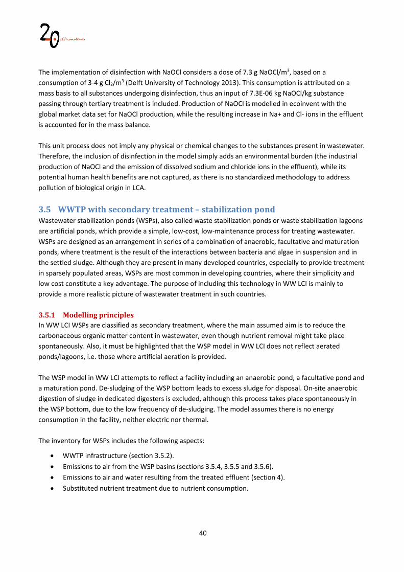
40

The implementation of disinfection with NaOCl considers a dose of 7.3 g NaOCl/m3, based on a consumption of 3-4 g Cl2/m3 (Delft University of Technology 2013). This consumption is attributed on a mass basis to all substances undergoing disinfection, thus an input of 7.3E-06 kg NaOCl/kg substance passing through tertiary treatment is included. Production of NaOCl is modelled in ecoinvent with the global market data set for NaOCl production, while the resulting increase in Na+ and Cl- ions in the effluent is accounted for in the mass balance. This unit process does not imply any physical or chemical changes to the substances present in wastewater. Therefore, the inclusion of disinfection in the model simply adds an environmental burden (the industrial production of NaOCl and the emission of dissolved sodium and chloride ions in the effluent), while its potential human health benefits are not captured, as there is no standardized methodology to address pollution of biological origin in LCA.

3.5 WWTP with secondary treatment – stabilization pond Wastewater stabilization ponds (WSPs), also called waste stabilization ponds or waste stabilization lagoons are artificial ponds, which provide a simple, low-cost, low-maintenance process for treating wastewater. WSPs are designed as an arrangement in series of a combination of anaerobic, facultative and maturation ponds, where treatment is the result of the interactions between bacteria and algae in suspension and in the settled sludge. Although they are present in many developed countries, especially to provide treatment in sparsely populated areas, WSPs are most common in developing countries, where their simplicity and low cost constitute a key advantage. The purpose of including this technology in WW LCI is mainly to provide a more realistic picture of wastewater treatment in such countries. 3.5.1 Modelling principles In WW LCI WSPs are classified as secondary treatment, where the main assumed aim is to reduce the carbonaceous organic matter content in wastewater, even though nutrient removal might take place spontaneously. Also, it must be highlighted that the WSP model in WW LCI does not reflect aerated ponds/lagoons, i.e. those where artificial aeration is provided. The WSP model in WW LCI attempts to reflect a facility including an anaerobic pond, a facultative pond and a maturation pond. De-sludging of the WSP bottom leads to excess sludge for disposal. On-site anaerobic digestion of sludge in dedicated digesters is excluded, although this process takes place spontaneously in the WSP bottom, due to the low frequency of de-sludging. The model assumes there is no energy consumption in the facility, neither electric nor thermal. The inventory for WSPs includes the following aspects:

WWTP infrastructure (section 3.5.2). Emissions to air from the WSP basins (sections 3.5.4, 3.5.5 and 3.5.6). Emissions to air and water resulting from the treated effluent (section 4). Substituted nutrient treatment due to nutrient consumption.

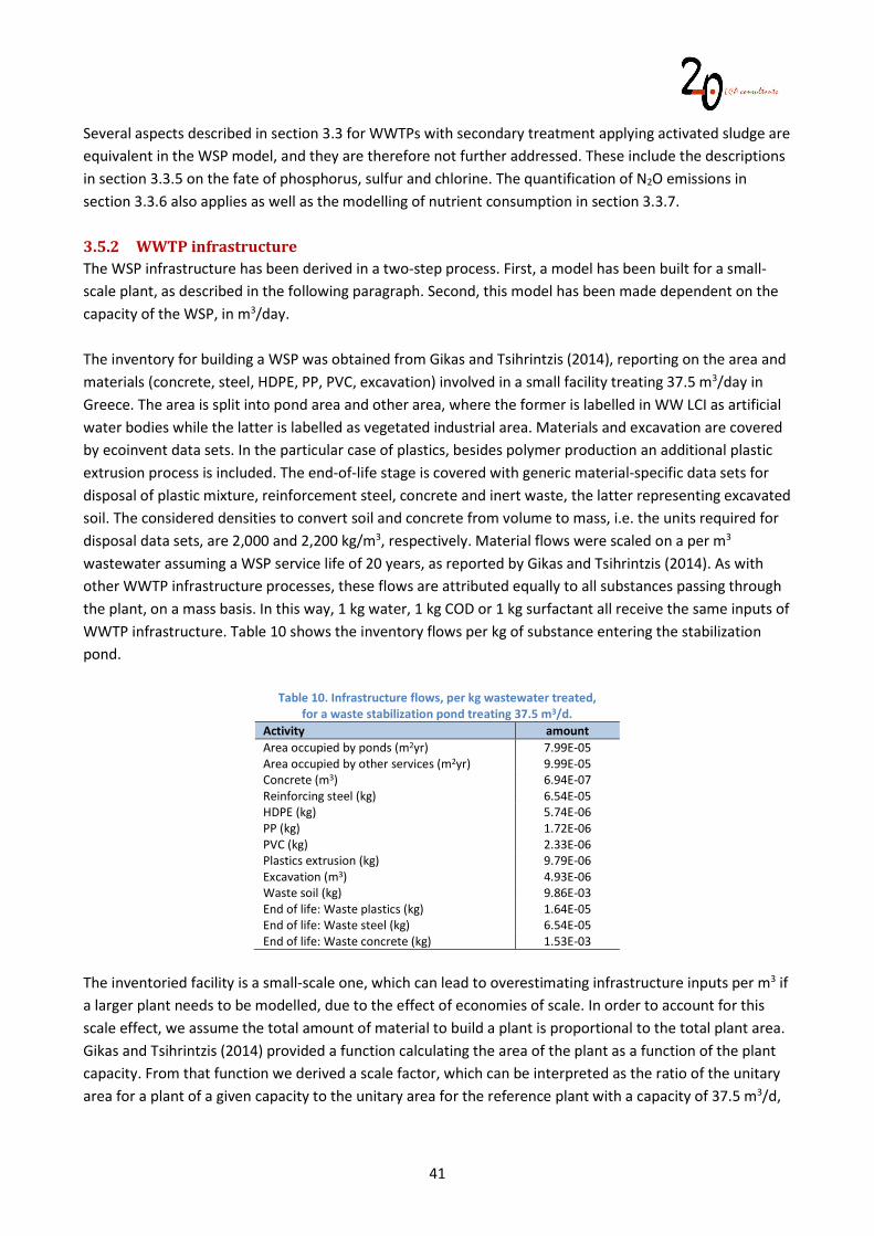
41

Several aspects described in section 3.3 for WWTPs with secondary treatment applying activated sludge are equivalent in the WSP model, and they are therefore not further addressed. These include the descriptions in section 3.3.5 on the fate of phosphorus, sulfur and chlorine. The quantification of N2O emissions in section 3.3.6 also applies as well as the modelling of nutrient consumption in section 3.3.7. 3.5.2 WWTP infrastructure The WSP infrastructure has been derived in a two-step process. First, a model has been built for a small-scale plant, as described in the following paragraph. Second, this model has been made dependent on the capacity of the WSP, in m3/day. The inventory for building a WSP was obtained from Gikas and Tsihrintzis (2014), reporting on the area and materials (concrete, steel, HDPE, PP, PVC, excavation) involved in a small facility treating 37.5 m3/day in Greece. The area is split into pond area and other area, where the former is labelled in WW LCI as artificial water bodies while the latter is labelled as vegetated industrial area. Materials and excavation are covered by ecoinvent data sets. In the particular case of plastics, besides polymer production an additional plastic extrusion process is included. The end-of-life stage is covered with generic material-specific data sets for disposal of plastic mixture, reinforcement steel, concrete and inert waste, the latter representing excavated soil. The considered densities to convert soil and concrete from volume to mass, i.e. the units required for disposal data sets, are 2,000 and 2,200 kg/m3, respectively. Material flows were scaled on a per m3 wastewater assuming a WSP service life of 20 years, as reported by Gikas and Tsihrintzis (2014). As with other WWTP infrastructure processes, these flows are attributed equally to all substances passing through the plant, on a mass basis. In this way, 1 kg water, 1 kg COD or 1 kg surfactant all receive the same inputs of WWTP infrastructure. Table 10 shows the inventory flows per kg of substance entering the stabilization pond.

Table 10. Infrastructure flows, per kg wastewater treated, for a waste stabilization pond treating 37.5 m3/d.

Activity amount Area occupied by ponds (m2yr) 7.99E-05 Area occupied by other services (m2yr) 9.99E-05 Concrete (m3) 6.94E-07 Reinforcing steel (kg) 6.54E-05 HDPE (kg) 5.74E-06 PP (kg) 1.72E-06 PVC (kg) 2.33E-06 Plastics extrusion (kg) 9.79E-06 Excavation (m3) 4.93E-06 Waste soil (kg) 9.86E-03 End of life: Waste plastics (kg) 1.64E-05 End of life: Waste steel (kg) 6.54E-05 End of life: Waste concrete (kg) 1.53E-03

The inventoried facility is a small-scale one, which can lead to overestimating infrastructure inputs per m3 if a larger plant needs to be modelled, due to the effect of economies of scale. In order to account for this scale effect, we assume the total amount of material to build a plant is proportional to the total plant area. Gikas and Tsihrintzis (2014) provided a function calculating the area of the plant as a function of the plant capacity. From that function we derived a scale factor, which can be interpreted as the ratio of the unitary area for a plant of a given capacity to the unitary area for the reference plant with a capacity of 37.5 m3/d,

42

where by unitary area we mean the area per m3 wastewater capacity (m2/m3/d). This scale factor is shown in Figure 9, where it can be seen that the bigger the plant, the lower this factor becomes, confirming the assumption of economies of scale. As an example, the area/m3 treated for a WSP with a capacity of 15,000 m3/d is only 30% of that for the reference plant treating 37.5 m3/d.

Figure 9. Waste stabilization pond infrastructure scale factor as a function of plant capacity. In this way, we calculate the infrastructure flows for a given WSP capacity with Equation 18: WSPinfra = 2.0421 · C-0.197 · WSPinfra-37.5

Equation 18. Calculation of infrastructure flows for waste stabilization ponds. Where WSPinfra is any of the infrastructure flows shown in Table 10, in kg or m2year per kg wastewater, adapted for a given WSP capacity C in m3/d. WSPinfra-37.5 corresponds to the same infrastructure flow, with the value for the reference plant treating 37.5 m3/d, shown in Table 10. 3.5.3 Fate factors In a Tier 1 assessment, the fate factors for wastewater components in a WSP are predefined, with the values shown in Table 11. The total removal for organic matter and suspended solids is set to 75%. This is based on a COD and SS removal of 70-83% and 73-83%, respectively, for WSPs including anaerobic, facultative and maturation ponds according to Von Sperling (2007c, table 4.9). For suspended organic and inorganic solids, this is assumed to be the result of settling, while for soluble organics the removal is associated with degradation. The remaining components water, ammonium, sulfate and phosphate do not require fate factors. The fate factors for metals are equivalent to those assumed for a WWTP with activated sludge (see section 3.3.3).

y = 2.0421x-0.197

00.10.20.30.40.50.60.70.80.9

1

0 3,000 6,000 9,000 12,000 15,000

WSP

scal

e fa

ctor

WSP capacity (m3/d)

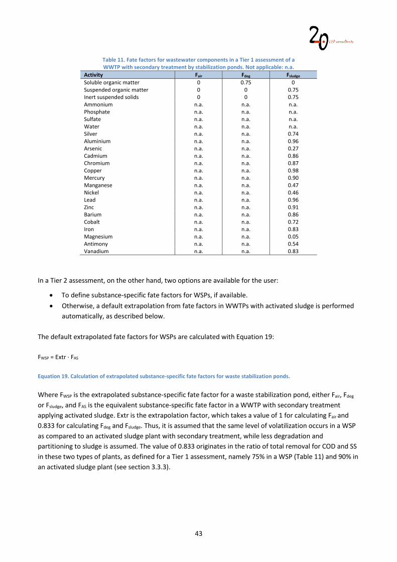
43

Table 11. Fate factors for wastewater components in a Tier 1 assessment of a WWTP with secondary treatment by stabilization ponds. Not applicable: n.a.

Activity Fair Fdeg Fsludge Soluble organic matter 0 0.75 0 Suspended organic matter 0 0 0.75 Inert suspended solids 0 0 0.75 Ammonium n.a. n.a. n.a. Phosphate n.a. n.a. n.a. Sulfate n.a. n.a. n.a. Water n.a. n.a. n.a. Silver n.a. n.a. 0.74 Aluminium n.a. n.a. 0.96 Arsenic n.a. n.a. 0.27 Cadmium n.a. n.a. 0.86 Chromium n.a. n.a. 0.87 Copper n.a. n.a. 0.98 Mercury n.a. n.a. 0.90 Manganese n.a. n.a. 0.47 Nickel n.a. n.a. 0.46 Lead n.a. n.a. 0.96 Zinc n.a. n.a. 0.91 Barium n.a. n.a. 0.86 Cobalt n.a. n.a. 0.72 Iron n.a. n.a. 0.83 Magnesium n.a. n.a. 0.05 Antimony n.a. n.a. 0.54 Vanadium n.a. n.a. 0.83

In a Tier 2 assessment, on the other hand, two options are available for the user:

To define substance-specific fate factors for WSPs, if available. Otherwise, a default extrapolation from fate factors in WWTPs with activated sludge is performed

automatically, as described below. The default extrapolated fate factors for WSPs are calculated with Equation 19: FWSP = Extr · FAS

Equation 19. Calculation of extrapolated substance-specific fate factors for waste stabilization ponds. Where FWSP is the extrapolated substance-specific fate factor for a waste stabilization pond, either Fair, Fdeg or Fsludge, and FAS is the equivalent substance-specific fate factor in a WWTP with secondary treatment applying activated sludge. Extr is the extrapolation factor, which takes a value of 1 for calculating Fair and 0.833 for calculating Fdeg and Fsludge. Thus, it is assumed that the same level of volatilization occurs in a WSP as compared to an activated sludge plant with secondary treatment, while less degradation and partitioning to sludge is assumed. The value of 0.833 originates in the ratio of total removal for COD and SS in these two types of plants, as defined for a Tier 1 assessment, namely 75% in a WSP (Table 11) and 90% in an activated sludge plant (see section 3.3.3).

44

3.5.4 Biological treatment: carbonaceous organic matter removal Degradation of soluble organic matter in a WSP relies on the same calculations described in section 3.3.4, i.e. the substance-specific fate factor Fdeg is used to quantify the extent of degradation, which is expected to take place mainly the facultative pond, while Equation 6 is used to represent the biochemical process. The only difference is the calculation of Yobs with Equation 7, where a different value for sludge residence time, c, is used. The reason is that WSPs have relatively longer residence times than conventional activated sludge plants. Given that a WSP does not recirculate activated sludge biomass, the sludge residence time equals the hydraulic residence time (HRT). Most of the aerobic degradation in such plants is expected to take place in the facultative ponds, since in anaerobic ponds settling prevails, while in maturation ponds the goal is not to remove BOD, but to remove pathogenic organisms. Thus, we have set HRT to reflect facultative pond conditions. According to Von Sperling (2007c), HRT for this type of plants is usually greater than 20 days. In WW LCI a value of 30 days is assumed. 3.5.5 Biological treatment: nitrogen removal Although not designed for N removal as such, several processes contribute to reducing the N load in the WSP effluent. These include volatilization, settling in bottom sludge and denitrification (Mayo 2013). The effectiveness of these systems in removing total N, though, is extremely variable in the literature. Von Sperling (2007c, table 4.9) considers 50-65% removal for this technology (anaerobic ponds followed by facultative and maturation ponds), which is consistent with several studies, reporting removal levels of 59% (Mayo 2013) and 64% (Hernández-Paniagua 2013). Other studies, though, report moderate removal levels of 7-24% (Paredes et al. 2015). In WW LCI, N removal in WSPs occurs through anaerobic degradation of settled sludge (see section 3.5.6), while in the water phase partial nitrification and denitrification is considered, using Equation 9 and Equation 11, respectively. As a default, a situation similar to that reported by Von Sperling (2016, table 14) is considered, where 43 monitored plants in Brazil applying anaerobic and facultative ponds showed an average N removal level of 39%. We achieve this with the following default factors:

For nitrification, ammonium-N conversion in Equation 9 is set to 75%. The remaining 25% is found in the treated effluent.

For denitrification, nitrate-N conversion in Equation 11 is set to 50%, while the remaining 50% nitrate-N is found in the treated effluent.

3.5.6 Anaerobic degradation of settled sludge Anaerobic degradation of organic matter in WSPs occurs mainly in the settled sludge, especially in anaerobic ponds, which are frequently used as primary settling units (Hernández-Paniagua 2013; Paing et al. 2003). In WW LCI, this process is modelled following the same procedure as in anaerobic digestion of sludge in a septic tank, as described in section 3.8.4, adapted here to reflect the specific sludge retention time in ponds, which is expected to be longer than in a (well maintained) septic tank, thus allowing for higher levels of sludge stabilization. A de-sludging frequency of 15 years is considered in the model. This is the value suggested by Picot et al. (2005) for WSPs in France, while Paing et al. (2003) suggests a value of 13 years. Based on the sludge stabilization curve developed for septic tanks (see Figure 10), this residence time leads to a reduction of 90% in volatile solids initially present in the settled sludge. This loss of volatile solids is modelled with the Buswell formula (Equation 1).

45

3.6 WWTP with primary treatment – conventional 3.6.1 Modelling principles The model for a WWTP with conventional primary treatment consists of mechanical pre-treatment followed by a primary settling tank. Sludge treatment consists of at least gravity thickening and dewatering. The model also considers optional anaerobic digestion of sludge, which is included depending on the scenario data. The inventory for this WWTP includes the following aspects:

WWTP infrastructure (section 3.6.2). Electricity balance (section 6.1). Thermal energy (natural gas and biogas) balance (section 6.2). Chemical reagents and auxiliary materials (polyelectrolyte for sludge conditioning, see section

5.1.4). Emissions to air and water resulting from the treated effluent (section 4). Emissions to air from combustion of biogas, if applicable (section 5.1.2).

3.6.2 WWTP infrastructure We did not find specific inventory data for infrastructure in WWTPs with primary treatment only. This is modelled with the same ecoinvent data sets shown in section 3.3.2. However, we attempt to take into account the fact that, for the same capacity, a plant with only primary treatment is likely to be require less infrastructure materials than a plant with secondary or tertiary treatment, which is what the ecoinvent data sets describe. This is due to the absence of, at least, the biological treatment basins and secondary settling tanks. In addition, as also discussed for secondary treatment, plants might include or not anaerobic digestion of sludge. For this type of plant, we perform a similar estimate as done in section 3.3.2 to determine the contribution of anaerobic digestion to the total plant infrastructure. The infrastructure of a plant with primary treatment and anaerobic digestion (InfraPRIM+AD) and without anaerobic digestion (InfraPRIM) is calculated as follows: InfraPRIM+AD = InfraAS+AD · 0.46 Equation 20. Calculation of infrastructure for a WWTP with primary treatment with anaerobic digestion of sludge. InfraPRIM = InfraAS+AD · 0.31 Equation 21. Calculation of infrastructure for a WWTP with primary treatment without anaerobic digestion of sludge. Where InfraAS+AD corresponds to the infrastructure of a WWTP applying secondary/tertiary treatment, as described by ecoinvent data sets of a particular WWTP class. The factor 0.46 results from the sum of infrastructure contributions in the Girona WWTP (Figure 7, left), excluding that of secondary treatment. The factor of 0.31 results from a similar sum, where the contribution of sludge treatment in that plant (0.18) is replaced by the contribution in the plant without anaerobic digestion (0.02, Figure 7, right). These figures seem to be in agreement with published data on investment costs, which are likely to be well correlated with material inputs to build a WWTP. COWI (2004) reports the investment cost of WWTPs with

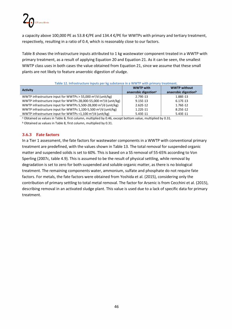
46

a capacity above 100,000 PE as 53.8 €/PE and 134.4 €/PE for WWTPs with primary and tertiary treatment, respectively, resulting in a ratio of 0.4, which is reasonably close to our factors. Table 8 shows the infrastructure inputs attributed to 1 kg wastewater component treated in a WWTP with primary treatment, as a result of applying Equation 20 and Equation 21. As it can be seen, the smallest WWTP class uses in both cases the value obtained from Equation 21, since we assume that these small plants are not likely to feature anaerobic digestion of sludge.

Table 12. Infrastructure inputs per kg substance in a WWTP with primary treatment.

Activity WWTP with

anaerobic digestiona WWTP without

anaerobic digestionb WWTP infrastructure input for WWTPs > 55,000 m3/d (unit/kg) 2.79E-13 1.88E-13 WWTP infrastructure input for WWTPs 28,000-55,000 m3/d (unit/kg) 9.15E-13 6.17E-13 WWTP infrastructure input for WWTPs 5,500-28,000 m3/d (unit/kg) 2.62E-12 1.76E-12 WWTP infrastructure input for WWTPs 1,100-5,500 m3/d (unit/kg) 1.22E-11 8.25E-12 WWTP infrastructure input for WWTPs <1,100 m3/d (unit/kg) 5.43E-11 5.43E-11 a Obtained as values in Table 8, first column, multiplied by 0.46, except bottom value, multiplied by 0.31. b Obtained as values in Table 8, first column, multiplied by 0.31.

3.6.3 Fate factors In a Tier 1 assessment, the fate factors for wastewater components in a WWTP with conventional primary treatment are predefined, with the values shown in Table 13. The total removal for suspended organic matter and suspended solids is set to 60%. This is based on a SS removal of 55-65% according to Von Sperling (2007c, table 4.9). This is assumed to be the result of physical settling, while removal by degradation is set to zero for both suspended and soluble organic matter, as there is no biological treatment. The remaining components water, ammonium, sulfate and phosphate do not require fate factors. For metals, the fate factors were obtained from Yoshida et al. (2015), considering only the contribution of primary settling to total metal removal. The factor for Arsenic is from Cecchini et al. (2015), describing removal in an activated sludge plant. This value is used due to a lack of specific data for primary treatment.

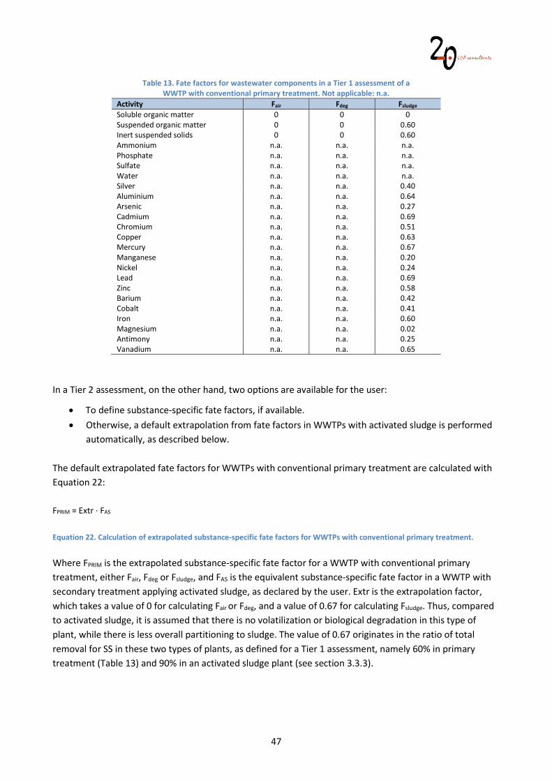
47

Table 13. Fate factors for wastewater components in a Tier 1 assessment of a WWTP with conventional primary treatment. Not applicable: n.a.

Activity Fair Fdeg Fsludge Soluble organic matter 0 0 0 Suspended organic matter 0 0 0.60 Inert suspended solids 0 0 0.60 Ammonium n.a. n.a. n.a. Phosphate n.a. n.a. n.a. Sulfate n.a. n.a. n.a. Water n.a. n.a. n.a. Silver n.a. n.a. 0.40 Aluminium n.a. n.a. 0.64 Arsenic n.a. n.a. 0.27 Cadmium n.a. n.a. 0.69 Chromium n.a. n.a. 0.51 Copper n.a. n.a. 0.63 Mercury n.a. n.a. 0.67 Manganese n.a. n.a. 0.20 Nickel n.a. n.a. 0.24 Lead n.a. n.a. 0.69 Zinc n.a. n.a. 0.58 Barium n.a. n.a. 0.42 Cobalt n.a. n.a. 0.41 Iron n.a. n.a. 0.60 Magnesium n.a. n.a. 0.02 Antimony n.a. n.a. 0.25 Vanadium n.a. n.a. 0.65

In a Tier 2 assessment, on the other hand, two options are available for the user:

To define substance-specific fate factors, if available. Otherwise, a default extrapolation from fate factors in WWTPs with activated sludge is performed

automatically, as described below. The default extrapolated fate factors for WWTPs with conventional primary treatment are calculated with Equation 22: FPRIM = Extr · FAS

Equation 22. Calculation of extrapolated substance-specific fate factors for WWTPs with conventional primary treatment. Where FPRIM is the extrapolated substance-specific fate factor for a WWTP with conventional primary treatment, either Fair, Fdeg or Fsludge, and FAS is the equivalent substance-specific fate factor in a WWTP with secondary treatment applying activated sludge, as declared by the user. Extr is the extrapolation factor, which takes a value of 0 for calculating Fair or Fdeg, and a value of 0.67 for calculating Fsludge. Thus, compared to activated sludge, it is assumed that there is no volatilization or biological degradation in this type of plant, while there is less overall partitioning to sludge. The value of 0.67 originates in the ratio of total removal for SS in these two types of plants, as defined for a Tier 1 assessment, namely 60% in primary treatment (Table 13) and 90% in an activated sludge plant (see section 3.3.3).

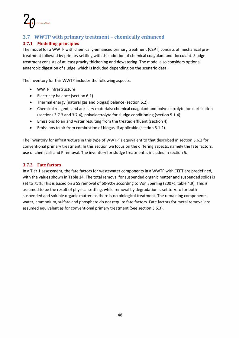
48

3.7 WWTP with primary treatment – chemically enhanced 3.7.1 Modelling principles The model for a WWTP with chemically-enhanced primary treatment (CEPT) consists of mechanical pre-treatment followed by primary settling with the addition of chemical coagulant and flocculant. Sludge treatment consists of at least gravity thickening and dewatering. The model also considers optional anaerobic digestion of sludge, which is included depending on the scenario data. The inventory for this WWTP includes the following aspects:

WWTP infrastructure Electricity balance (section 6.1). Thermal energy (natural gas and biogas) balance (section 6.2). Chemical reagents and auxiliary materials: chemical coagulant and polyelectrolyte for clarification

(sections 3.7.3 and 3.7.4), polyelectrolyte for sludge conditioning (section 5.1.4). Emissions to air and water resulting from the treated effluent (section 4) Emissions to air from combustion of biogas, if applicable (section 5.1.2).

The inventory for infrastructure in this type of WWTP is equivalent to that described in section 3.6.2 for conventional primary treatment. In this section we focus on the differing aspects, namely the fate factors, use of chemicals and P removal. The inventory for sludge treatment is included in section 5. 3.7.2 Fate factors In a Tier 1 assessment, the fate factors for wastewater components in a WWTP with CEPT are predefined, with the values shown in Table 14. The total removal for suspended organic matter and suspended solids is set to 75%. This is based on a SS removal of 60-90% according to Von Sperling (2007c, table 4.9). This is assumed to be the result of physical settling, while removal by degradation is set to zero for both suspended and soluble organic matter, as there is no biological treatment. The remaining components water, ammonium, sulfate and phosphate do not require fate factors. Fate factors for metal removal are assumed equivalent as for conventional primary treatment (See section 3.6.3).

49

Table 14. Fate factors for wastewater components in a Tier 1 assessment of a

WWTP with chemically-enhanced primary treatment. Not applicable: n.a. Activity Fair Fdeg Fsludge Soluble organic matter 0 0 0 Suspended organic matter 0 0 0.75 Inert suspended solids 0 0 0.75 Ammonium n.a. n.a. n.a. Phosphate n.a. n.a. n.a. Sulfate n.a. n.a. n.a. Water n.a. n.a. n.a. Silver n.a. n.a. 0.40 Aluminium n.a. n.a. 0.64 Arsenic n.a. n.a. 0.27 Cadmium n.a. n.a. 0.69 Chromium n.a. n.a. 0.51 Copper n.a. n.a. 0.63 Mercury n.a. n.a. 0.67 Manganese n.a. n.a. 0.20 Nickel n.a. n.a. 0.24 Lead n.a. n.a. 0.69 Zinc n.a. n.a. 0.58 Barium n.a. n.a. 0.42 Cobalt n.a. n.a. 0.41 Iron n.a. n.a. 0.60 Magnesium n.a. n.a. 0.02 Antimony n.a. n.a. 0.25 Vanadium n.a. n.a. 0.65

In a Tier 2 assessment, on the other hand, two options are available for the user:

To define substance-specific fate factors, if available. Otherwise, a default extrapolation from fate factors in WWTPs with activated sludge is performed

automatically, as described below. The default extrapolated fate factors for WWTPs with conventional primary treatment are calculated with Equation 23: FPRIM-CE = Extr · FAS

Equation 23. Calculation of extrapolated substance-specific fate factors for WWTPs with chemically-enhanced primary treatment. Where FPRIM-CE is the extrapolated substance-specific fate factor for a WWTP with chemically-enhanced primary treatment, either Fair, Fdeg or Fsludge, and FAS is the equivalent substance-specific fate factor in a WWTP with secondary treatment applying activated sludge, as declared by the user. Extr is the extrapolation factor, which takes a value of 0 for calculating Fair or Fdeg, and a value of 0.83 for calculating Fsludge. Thus, compared to activated sludge, it is assumed that there is no volatilization or biological degradation in this type of plant, while there is less overall partitioning to sludge. The value of 0.83 originates in the ratio of total removal for SS in these two types of plants, as defined for a Tier 1 assessment, namely 75% in CEPT (Table 14) and 90% in an activated sludge plant (see section 3.3.3).

50

3.7.3 Phosphorus removal Chemically-enhanced primary treatment is expected to achieve higher P removal levels than conventional primary treatment, due to the use of coagulation and flocculation. On the one hand, this leads to higher suspended solids removal, thus increasing the amount of suspended P that can be removed. On the other hand, coagulants such as ferric chloride can precipitate dissolved orthophosphate, in the same way as considered for WWTPs with tertiary treatment (see section 3.4.5). In this section we account for this second effect, given that removal of suspended solids has already been addressed in section 3.7.2. According to Von Sperling (2007c, table 4.9) CEPT is capable of removing 75-90% of total P in wastewater. However, published data for two real plants applying this type of treatment, namely El Salitre WWTP in Bogotá, Colombia (Kingsley 2011) and the Point Loma WWTP in San Diego, United States (City of San Diego 2005, 2008, 2016) suggests a lower performance. In El Salitre WWTP, total P removal is reported as 38%. In Point Loma WWTP this parameter is not reported, but orthophosphate removal is reported as 10%. Based on its suspended solids removal (around 90%), we estimate that total P removal in Point Loma might also be around 30-40%. In WW LCI, P removal in CEPT is modelled following the same procedure described for WWTPs with tertiary treatment in section 3.4.5, that is, chemical precipitation of dissolved orthophosphate, although we assume a lower overall removal level, namely that 25% of PO4-P is removed by this process, instead of the default 80% considered in tertiary treatment. This 25% PO4-P removal, added to the suspended P removal implicit in settling of suspended solids, leads to an overall P removal which is along the lines reported at the two real plants. It must be highlighted that in WW LCI, PO4-P removal incurs in its own consumption of ferric chloride and production of sludge, as explained in section 3.4.5. 3.7.4 Use of chemicals The inventory for chemically-enhanced primary treatment includes consumption of ferric chloride and polyelectrolyte to improve removal of suspended solids. Consumption of chemicals during CEPT is quantified as a function of the amount of substance removed by settling, which is in turn defined by the fate factor Fsludge, calculated as described in section 3.6.3. The unitary consumption, in kg chemical per kg solids removed has been derived from published data for two real plants applying this type of treatment, namely El Salitre WWTP in Bogotá, Colombia (Kingsley 2011) and the Point Loma WWTP in San Diego, United States (City of San Diego 2005, 2008, 2016). Table 15 shows the data from these two plants, in particular the total suspended solids in influent and effluent and the consumption of chemicals. In the particular case of the Point Loma WWTP, we show the data for 2004 and 2007, before the plant installed a system for hydrogen sulfide control, which doses, among other chemicals, ferrous chloride. As a result of this system, the dose of ferric chloride as coagulant was substantially reduced. Thus, the data we show reflect the standard operation of a chemically-enhanced primary treatment, without the influence of the additional hydrogen sulfide control system. In WW LCI we use a unitary consumption calculated as the arithmetic average of the two plants, namely 0.15 kg ferric chloride/kg SS removed and 0.002 kg polyelectrolyte/kg solids removed. Polyelectrolyte production is approximated with the ecoinvent market data set for acrylamide.

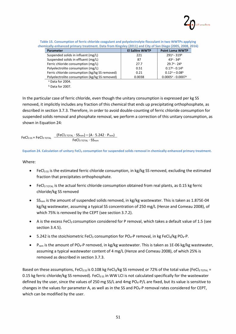
51

Table 15. Consumption of ferric chloride coagulant and polyelectrolyte flocculant in two WWTPs applying

chemically-enhanced primary treatment. Data from Kingsley (2011) and City of San Diego (2005, 2008, 2016) Parameter El Salitre WWTP Point Loma WWTP Suspended solids in influent (mg/L) 221 291a - 319b

Suspended solids in effluent (mg/L) 87 43a - 34b Ferric chloride consumption (mg/L) 27.7 29.7a - 24b Polyelectrolite consumption (mg/L) 0.51 0.17a - 0.14b Ferric chloride consumption (kg/kg SS removed) 0.21 0.12a – 0.08b

Polyelectrolite consumption (kg/kg SS removed) 0.0038 0.0005a - 0.0007a a Data for 2004. b Data for 2007.

In the particular case of ferric chloride, even though the unitary consumption is expressed per kg SS removed, it implicitly includes any fraction of this chemical that ends up precipitating orthophosphate, as described in section 3.7.3. Therefore, in order to avoid double-counting of ferric chloride consumption for suspended solids removal and phosphate removal, we perform a correction of this unitary consumption, as shown in Equation 24:

FeCl3 SS = FeCl3 TOTAL (FeCl3 TOTAL · SSrem) – (A · 5.242 · Prem)

FeCl3 TOTAL · SSrem Equation 24. Calculation of unitary FeCl3 consumption for suspended solids removal in chemically-enhanced primary treatment. Where:

FeCl3 SS is the estimated ferric chloride consumption, in kg/kg SS removed, excluding the estimated fraction that precipitates orthophosphate.

FeCl3 TOTAL is the actual ferric chloride consumption obtained from real plants, as 0.15 kg ferric chloride/kg SS removed

SSrem is the amount of suspended solids removed, in kg/kg wastewater. This is taken as 1.875E-04 kg/kg wastewater, assuming a typical SS concentration of 250 mg/L (Henze and Comeau 2008), of which 75% is removed by the CEPT (see section 3.7.2).

A is the excess FeCl3 consumption considered for P removal, which takes a default value of 1.5 (see section 3.4.5).

5.242 is the stoichiometric FeCl3 consumption for PO4-P removal, in kg FeCl3/kg PO4-P.

Prem is the amount of PO4-P removed, in kg/kg wastewater. This is taken as 1E-06 kg/kg wastewater, assuming a typical wastewater content of 4 mg/L (Henze and Comeau 2008), of which 25% is removed as described in section 3.7.3.

Based on these assumptions, FeCl3 SS is 0.108 kg FeCl3/kg SS removed, or 72% of the total value (FeCl3 TOTAL = 0.15 kg ferric chloride/kg SS removed). FeCl3 SS in WW LCI is not calculated specifically for the wastewater defined by the user, since the values of 250 mg SS/L and 4mg PO4-P/L are fixed, but its value is sensitive to changes in the values for parameter A, as well as in the SS and PO4-P removal rates considered for CEPT, which can be modified by the user.

52

The addition of ferric chloride and polyelectrolyte in CEPT contributes to the formation of primary sludge. In the model, polyelectrolyte is entirely partitioned to sludge, while ferric chloride dissociates to Cl- and Fe3+ ions. The former are found in the treated effluent, while Fe3+ is assumed to precipitate as Fe(OH)3. Based on stoichiometry, each kg FeCl3 added in primary treatment requires an input of 0.314 kg OH- ions and results in 0.658 kg Fe(OH)3 and 0.655 kg Cl-. The input of OH- ions is only reflected in the mass balance, but is not part of the LCI.

3.8 Septic tanks A septic tank is an underground chamber made of concrete, fiberglass, or plastic through which domestic wastewater flows, providing basic treatment, namely reduction of suspended solids and anaerobic degradation of these at the bottom of the tank. 3.8.1 Modelling principles In WW LCI, septic tanks are modelled as systems with independent collection of wastewater, i.e. not connected to a public sewer. The septic tank model includes the biochemical processes taking place in water and settled solids, while eventual de-sludging leads to excess sludge for disposal. The model assumes that the treated effluent is discharged to groundwater and that no energy consumption is involved in the operation of these systems. The inventory for septic tanks includes the following aspects:

Septic tank infrastructure (section 3.8.2). Emissions to air and water resulting from the treated effluent (section 4). Emissions to air from the septic tank (section 3.8.4).

Disposal of sludge generated in septic tanks is described in section 5. 3.8.2 Septic tank infrastructure Inventory data on construction of a septic tank has been obtained from from Magar (2016) describing a septic tank installed in Norway, for an average capacity of 8 PE (1,600 L/d). The LCI data available in this study covers the septic tank as a primary treatment, plus other more advanced unit operations, however we focused on the septic tank only. The study provides the total amount of materials, which are assumed by the author to have a life span of 20 years. The excavated volume was not originally quantified; we added this as the volume of the tank itself (9.5 m3) plus the volume occupied by the surrounding gravel (7 m3). All activities are covered with ecoinvent data sets. In the case of the geomembrane, this was modelled as HDPE. We added a pipe extrusion process to approximate the manufacturing of the pipe and geomembrane. The end-of-life stage of the septic tank is included following the same procedure described for waste stabilization pond infrastructure in section 3.5.2. The inventory for septic tank infrastructure is summarized in Table 16. In the same way as for other infrastructure related to wastewater collection and treatment in WW LCI, these flows are attributed to wastewater components on a mass basis.

53

Table 16. Infrastructure flows, per kg wastewater treated, for a septic tank. Based on Magar (2016). Activity amount Polyvinyl chloride (kg) 1.05E-05 Geomembrane (as high-density polyethylene) (kg) 2.91E-06 Glass fibre (kg) 3.25E-05 Gravel (kg) 9.09E-04 Excavation (m3) 1.41E-06 Plastics extrusion (kg) 1.34E-05 Waste soil (kg) 2.82E-03 End of life: Waste plastics (kg) 1.34E-05 End of life: Waste gravel (kg) 9.00E-04 End of life: Waste glass fibre (kg) 3.25E-05

3.8.3 Fate factors In a Tier 1 assessment, the fate factors for wastewater components in a septic tank are predefined, with the values shown in Table 17. The total removal for suspended organic matter and suspended inert solids is set to 60%. This is based on a SS removal of 55-65% according to Von Sperling (2007c, table 4.9). This is assumed to be the result of physical settling, while removal by degradation is set to zero for both suspended and soluble organic matter, as we assume there is no biological activity in the water phase. The remaining components water, ammonium, sulfate and phosphate do not require fate factors. Fate factors for metal removal are assumed equivalent as for conventional primary treatment (see section 3.6.3).

Table 17. Fate factors for wastewater components in a Tier 1 assessment of a septic tank. Not applicable: n.a. Activity Fair Fdeg Fsludge Soluble organic matter 0 0 0 Suspended organic matter 0 0 0.60 Inert suspended solids 0 0 0.60 Ammonium n.a. n.a. n.a. Phosphate n.a. n.a. n.a. Sulfate n.a. n.a. n.a. Water n.a. n.a. n.a. Silver n.a. n.a. 0.40 Aluminium n.a. n.a. 0.64 Arsenic n.a. n.a. 0.27 Cadmium n.a. n.a. 0.69 Chromium n.a. n.a. 0.51 Copper n.a. n.a. 0.63 Mercury n.a. n.a. 0.67 Manganese n.a. n.a. 0.20 Nickel n.a. n.a. 0.24 Lead n.a. n.a. 0.69 Zinc n.a. n.a. 0.58 Barium n.a. n.a. 0.42 Cobalt n.a. n.a. 0.41 Iron n.a. n.a. 0.60 Magnesium n.a. n.a. 0.02 Antimony n.a. n.a. 0.25 Vanadium n.a. n.a. 0.65

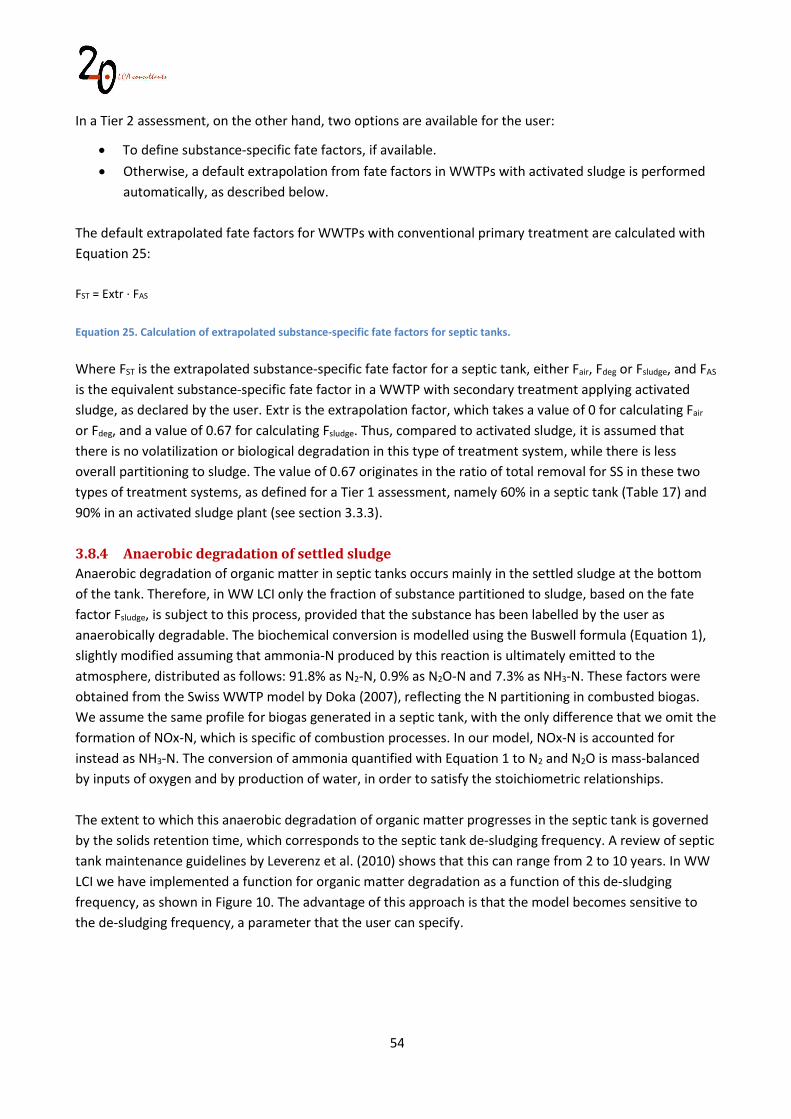
54

In a Tier 2 assessment, on the other hand, two options are available for the user:

To define substance-specific fate factors, if available. Otherwise, a default extrapolation from fate factors in WWTPs with activated sludge is performed

automatically, as described below. The default extrapolated fate factors for WWTPs with conventional primary treatment are calculated with Equation 25: FST = Extr · FAS

Equation 25. Calculation of extrapolated substance-specific fate factors for septic tanks. Where FST is the extrapolated substance-specific fate factor for a septic tank, either Fair, Fdeg or Fsludge, and FAS is the equivalent substance-specific fate factor in a WWTP with secondary treatment applying activated sludge, as declared by the user. Extr is the extrapolation factor, which takes a value of 0 for calculating Fair

or Fdeg, and a value of 0.67 for calculating Fsludge. Thus, compared to activated sludge, it is assumed that there is no volatilization or biological degradation in this type of treatment system, while there is less overall partitioning to sludge. The value of 0.67 originates in the ratio of total removal for SS in these two types of treatment systems, as defined for a Tier 1 assessment, namely 60% in a septic tank (Table 17) and 90% in an activated sludge plant (see section 3.3.3). 3.8.4 Anaerobic degradation of settled sludge Anaerobic degradation of organic matter in septic tanks occurs mainly in the settled sludge at the bottom of the tank. Therefore, in WW LCI only the fraction of substance partitioned to sludge, based on the fate factor Fsludge, is subject to this process, provided that the substance has been labelled by the user as anaerobically degradable. The biochemical conversion is modelled using the Buswell formula (Equation 1), slightly modified assuming that ammonia-N produced by this reaction is ultimately emitted to the atmosphere, distributed as follows: 91.8% as N2-N, 0.9% as N2O-N and 7.3% as NH3-N. These factors were obtained from the Swiss WWTP model by Doka (2007), reflecting the N partitioning in combusted biogas. We assume the same profile for biogas generated in a septic tank, with the only difference that we omit the formation of NOx-N, which is specific of combustion processes. In our model, NOx-N is accounted for instead as NH3-N. The conversion of ammonia quantified with Equation 1 to N2 and N2O is mass-balanced by inputs of oxygen and by production of water, in order to satisfy the stoichiometric relationships. The extent to which this anaerobic degradation of organic matter progresses in the septic tank is governed by the solids retention time, which corresponds to the septic tank de-sludging frequency. A review of septic tank maintenance guidelines by Leverenz et al. (2010) shows that this can range from 2 to 10 years. In WW LCI we have implemented a function for organic matter degradation as a function of this de-sludging frequency, as shown in Figure 10. The advantage of this approach is that the model becomes sensitive to the de-sludging frequency, a parameter that the user can specify.

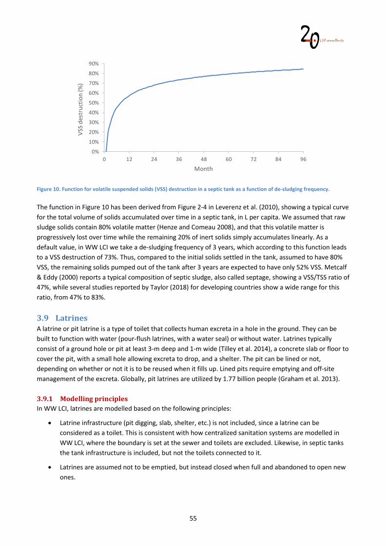
55

Figure 10. Function for volatile suspended solids (VSS) destruction in a septic tank as a function of de-sludging frequency. The function in Figure 10 has been derived from Figure 2-4 in Leverenz et al. (2010), showing a typical curve for the total volume of solids accumulated over time in a septic tank, in L per capita. We assumed that raw sludge solids contain 80% volatile matter (Henze and Comeau 2008), and that this volatile matter is progressively lost over time while the remaining 20% of inert solids simply accumulates linearly. As a default value, in WW LCI we take a de-sludging frequency of 3 years, which according to this function leads to a VSS destruction of 73%. Thus, compared to the initial solids settled in the tank, assumed to have 80% VSS, the remaining solids pumped out of the tank after 3 years are expected to have only 52% VSS. Metcalf & Eddy (2000) reports a typical composition of septic sludge, also called septage, showing a VSS/TSS ratio of 47%, while several studies reported by Taylor (2018) for developing countries show a wide range for this ratio, from 47% to 83%.

3.9 Latrines A latrine or pit latrine is a type of toilet that collects human excreta in a hole in the ground. They can be built to function with water (pour-flush latrines, with a water seal) or without water. Latrines typically consist of a ground hole or pit at least 3-m deep and 1-m wide (Tilley et al. 2014), a concrete slab or floor to cover the pit, with a small hole allowing excreta to drop, and a shelter. The pit can be lined or not, depending on whether or not it is to be reused when it fills up. Lined pits require emptying and off-site management of the excreta. Globally, pit latrines are utilized by 1.77 billion people (Graham et al. 2013). 3.9.1 Modelling principles In WW LCI, latrines are modelled based on the following principles:

Latrine infrastructure (pit digging, slab, shelter, etc.) is not included, since a latrine can be considered as a toilet. This is consistent with how centralized sanitation systems are modelled in WW LCI, where the boundary is set at the sewer and toilets are excluded. Likewise, in septic tanks the tank infrastructure is included, but not the toilets connected to it.

Latrines are assumed not to be emptied, but instead closed when full and abandoned to open new ones.

0%

10%

20%

30%

40%

50%

60%

70%

80%

90%

0 12 24 36 48 60 72 84 96

VSS

dest

ruct

ion

(%)

Month

56

The pollutant load remaining in the pit is inventoried as emissions to groundwater.

Human excreta is assumed to be flushed with water, even though latrines are often dry. In WW LCI, discharges through latrines are attributed emissions to air and water resulting from the degradation of human excreta. The specific calculations are described in section 4. In this section we focus instead on defining a site-specific methane correction factor for latrines (MCFlat), which determines the extent to which degradation of human excreta in latrines is expected to occur under anaerobic conditions. 3.9.2 Methane correction factor for latrines (MCFlat) Doorn and Liles (1999) considered latrines to be fully anaerobic, which corresponds to an MCF of 1. In the IPCC Guidelines for National Greenhouse-gas inventories (Doorn et al. 2006) this was further detailed depending on climate and latrine design and management. On the one hand, latrines in dry climates or with a water table below the latrine, or with regular emptying, received an MCF of 0.1 (ranging from 0.05 to 0.15), increased to 0.5 (range 0.4 to 0.6) in case of communal latrines. On the other hand, latrines either in wet climates or with a pour-flush system, or with the water table above the latrine bottom, received an MCF of 0.7 (ranging from 0.7 to 1). Reid et al. (2014) used these MCFs to conduct a detailed analysis of methane emissions from latrines in 21 countries, focusing on rural population and taking into account site-specific water table depths. Although they do not report country-specific MCFs for latrines as part of their results, they present country-specific emission factors expressed as kg methane/kg BOD. Since they consider the maximum methane production capacity for 1 kg BOD is 0.6 kg methane, their emission factors can be expressed as MCFs after dividing by 0.6. Their (implicit) country-specific MCFs range from 0.12 for South Africa to 0.64 for Bangladesh. Although these factors can be used straightaway in WW LCI, the limitation is that only 21 countries are covered, while WW LCI aims at providing global coverage. For this reason, in WW LCI we have opted for developing a simple approach to determine country-specific methane correction factors for latrines (MCFlat) that takes into account climatic conditions only. MCFlat is defined as a function of dry or wet conditions, which are characterized in the model by mean annual precipitation. A MCFlat = 0.1 is chosen for the driest country and a MCFlat = 0.7 is chosen for the country with the highest precipitation. A linear relationship is assumed. Based on statistics from the World Bank (2020a) in 2014, the driest country is Egypt (51 mm/year) and Colombia is the one with the highest precipitation (3,240 mm/year). With these four data points, MCFlat can be calculated for any country with Equation 26: MCFlat = 0.000188147x + 0.090404516 Equation 26. Calculation of the methane correction factor for latrines. Where x is precipitation, in mm/year. As a quick sanity check, Equation 26 attributes Bangladesh (2,666 mm/year) with an MCFlat = 0.59 and South Africa (495 mm/year) with an MCFlat = 0.18, reasonably close to the factors from Reid et al. (2014).

3.10 Open defecation Open defecation is the practice of defecating outdoors, such as in fields, forests, bushes, lakes and rivers, without the use of any kind of toilet facility. Globally, the practice is decreasing steadily, but still close to

57

700 million people practice open defecation, especially in rural areas in Africa (UN News 2019). Elimination of this practice by 2030 constitutes one of the targets of the Sustainable Development Goals (SDGs). 3.10.1 Modelling principles In WW LCI, open defecation is attributed emissions to air resulting from the degradation of human excreta. Defecation is assumed to take place on land, therefore excreta are assumed to constitute an emission to soil. A current limitation of the model for open defecation is that in a Tier 1 assessment the inventory considers that human excreta are flushed with water, as it would be in a toilet. In a Tier 2 assessment, though, it is possible to conduct a specific assessment of human excreta by defining its composition and water content. The specific emission calculations are described in section 4. In this section we focus instead on defining a generic methane correction factor for open defecation (MCFdef), which determines the extent to which degradation of human excreta in these circumstances is expected to occur under anaerobic conditions. 3.10.2 Methane correction factor for open defecation (MCFdef) The IPCC Guidelines for National Greenhouse-gas inventories (Doorn et al. 2006) did not include open defecation as a source of methane emissions, and therefore an MCF for this activity was not provided. The only study we have found quantifying methane from open defecation was carried out by Winrock (2008), reporting a 30-day experiment in India to measure methane production by a sample of night soil. In WW LCI we have used the results of this study to derive a generic MCF for open defecation (MCFopen), calculated with Equation 27:

MCFdef = ProdCH4 · 12

Prodfec · Cfec · dmfec · fCH4 · 16 Equation 27. Calculation of a methane correction factor for open defecation. Where:

ProdCH4 is the methane production according to the experiment by Winrock (2008), a total of 0.00952 kg in 30 days.

Prodfec is the wet weight of the sample used in the experiment by Winrock (2008), a total of 2.2 kg.

Cfec is the carbon content in faeces, in kg carbon per kg dry mass. This is taken as 0.5 from Feachem et al. (1983).

dmfec is the dry mass content in faeces. This is taken as 0.25 kg dry mass per kg wet mass Feachem et al. (1983).

fCH4 is the fraction of carbon converted to methane during anaerobic degradation. This is taken as 0.6 from Muñoz et al. (2013).

Under these assumptions MCFdef is estimated at 0.043. This is lower than the best case for latrines, with an MCF of 0.1 in dry climates or low water tables, according to Doorn et al. (2006). This seems reasonable, given that latrines, even when correctly managed, are more likely to present anaerobic conditions than

58

open defecation, given that the former accumulate higher volumes of excreta, making air flow and thus aerobic conditions more difficult than single defecation events in the open.

59

4 Wastewater and excreta discharged to the environment In this section we address the emissions to air, water and soil resulting from discharges of wastewater and human excreta coming from the following sources:

Untreated wastewater from closed sewers not connected to WWTPs. Untreated wastewater from open, stagnant sewers. Treated effluent from WWTPs with either primary, secondary or tertiary treatment. Treated effluent from septic tanks. Discharges of human excreta through latrines. Discharges of human excreta through open defecation. Volatilization of substances from WWTPs or from sludge composting plants.

4.1 Direct emissions When a substance is discharged in wastewater or as part of human excreta, this is directly reported in the inventory, as an emission to either freshwater, seawater, groundwater or soil, depending on the scenario conditions. In addition, if the substance is organic, it is also reported in the inventory as COD, the latter calculated based on the following chemical reaction (Wikipedia 2018): CnHaObNc + (n + a/4 – b/2 – 3/4 c) O2 → n CO2 + (a/2 – 3/2 c) H2O + c NH3 Equation 28. chemical oxidation of organic matter. This oxidation does not include the COD from oxidation of ammonia to nitrate, since dichromate (the chemical reagent used for COD determination) does not oxidize ammonia. COD is calculated in kg O2/kg for a given organic substance with Equation 29, while it is zero for inorganic substances:

COD = 32 (n + 0.25 a + 0.5 b - 0.75 c)

MW Equation 29. Calculation of the chemical oxygen demand. Where n, a, b and c correspond to the sub-indexes shown in Equation 28 and MW is the molecular weight of the chemical substance, in g/mol. Besides the direct emission of substances to the receiving compartments, WW LCI addresses the indirect emissions resulting from eventual degradation of these substances in these compartments, as described in the following sections.

4.2 Indirect emissions As mentioned in section 2.6, WW LCI addresses not only what is discharged to the environment, but also emissions as a result of chemical substances in these discharges breaking down into different relevant degradation products such as CO2, methane and nutrients, among others.

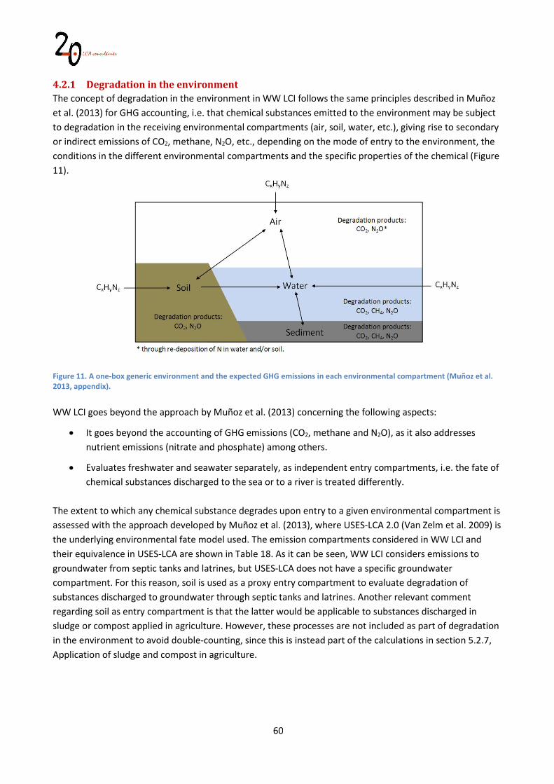
60

4.2.1 Degradation in the environment The concept of degradation in the environment in WW LCI follows the same principles described in Muñoz et al. (2013) for GHG accounting, i.e. that chemical substances emitted to the environment may be subject to degradation in the receiving environmental compartments (air, soil, water, etc.), giving rise to secondary or indirect emissions of CO2, methane, N2O, etc., depending on the mode of entry to the environment, the conditions in the different environmental compartments and the specific properties of the chemical (Figure 11).

Figure 11. A one-box generic environment and the expected GHG emissions in each environmental compartment (Muñoz et al. 2013, appendix). WW LCI goes beyond the approach by Muñoz et al. (2013) concerning the following aspects:

It goes beyond the accounting of GHG emissions (CO2, methane and N2O), as it also addresses nutrient emissions (nitrate and phosphate) among others.

Evaluates freshwater and seawater separately, as independent entry compartments, i.e. the fate of chemical substances discharged to the sea or to a river is treated differently.

The extent to which any chemical substance degrades upon entry to a given environmental compartment is assessed with the approach developed by Muñoz et al. (2013), where USES-LCA 2.0 (Van Zelm et al. 2009) is the underlying environmental fate model used. The emission compartments considered in WW LCI and their equivalence in USES-LCA are shown in Table 18. As it can be seen, WW LCI considers emissions to groundwater from septic tanks and latrines, but USES-LCA does not have a specific groundwater compartment. For this reason, soil is used as a proxy entry compartment to evaluate degradation of substances discharged to groundwater through septic tanks and latrines. Another relevant comment regarding soil as entry compartment is that the latter would be applicable to substances discharged in sludge or compost applied in agriculture. However, these processes are not included as part of degradation in the environment to avoid double-counting, since this is instead part of the calculations in section 5.2.7, Application of sludge and compost in agriculture.

61

Table 18. Emission compartments in WW LCI and equivalence in USES-LCA. Emission compartment in WW LCI Activity generating emission Emission compartment in USES-LCA

Air Volatilization in WWTPs Composting

Air

Freshwater Treated wastewater discharges Untreated wastewater discharges

Freshwater

Seawater Treated wastewater discharges Untreated wastewater discharges

Seawater

Groundwater Effluent from septic tanks Latrines

Soil

Soil Open defecation Nonea a Soil would also be the compartment of choice for substances present in compost or sludge applied in agriculture, however these processes are not included under degradation in the environment, but under section 5.2.7. Application of sludge and compost in agriculture.

For a given chemical substance emitted to either air, freshwater, seawater or soil, USES-LCA is used to predict the fraction expected to degrade in the different environmental compartments (air, water, soil, sediments), as a result of multi-media distribution and degradability. Thus, from USES-LCA we obtain the following parameters:

Dega: fraction degraded in the atmosphere. Degw: fraction degraded in freshwater and seawater. Degs: fraction degraded in soil. Degsed: fraction degraded in freshwater and seawater sediments.

The values for the above parameters are substance-specific, but also for a given substance they vary according to the emission compartment. As an example, Table 19 shows the degradation profile for ethanol emitted to each of the considered entry compartments: air, freshwater, seawater and soil. It must be highlighted that the sum of the four parameters might not always add up to 100%, meaning that a fraction of the substance is ‘removed’ from the system. This is the case for extremely persistent chemicals being for example buried in sediments. In the case of ethanol, as seen in Table 19, this removal is negligible.

Table 19. Distribution of degradation in the environment for ethanol, by emission compartment in USES-LCA. Emission compartment Degair Degw Degsed Degs Sum Air 42.61% 56.25% 0.00% 1.13% 99.99% Freshwater 13.14% 86.45% 0.05% 0.35% 99.99% Soil 23.15% 36.85% 0.00% 39.98% 99.98% Seawater 0.95% 99.02% 0.00% 0.03% 100.00%

The potential products considered as a result of degradation in the environment are shown in Table 20. This table shows the chemical species in which C, N, P, S and Cl originally present in the degraded substances are expected to be found. The fate of N, P, S and Cl after degradation in the atmosphere was defined based on a personal communication with Prof. Xavier Domènech (Domènech 2020).

62

Table 20. Chemical speciation considered for degradation in the environment. Element in parent substance Substance degraded in air Substance degraded in water, soil or sediments Carbon CO2 to air CO2 to air, CH4 to air Nitrogen NOx, N2O to air NO3 to water, N2O to air Phosphorus P2O5 to air PO4 to water Sulfur SO2 to air H2S to air, SO4 to water Chlorine HCl to air Cl to water Emissions of methane and hydrogen sulfide are only calculated when degradation occurs under anaerobic conditions. The extent of such anaerobic conditions in these media are determined by the different methane correction factors (MCF). Figure 12 summarizes which MCF applies in which case. The determination of MCFopen, MCFlat and MCFdef has been described in sections 3.2.3, 3.9.2 and 3.10.2, respectively, while MCFsed and MCFw are described in the following sections.

Fraction degraded in water (Degw)

MCFw MCFw MCFw MCFw MCFopen MCFlat MCFdef

Fraction degraded in sediments (Degsed)

MCFsed MCFsed MCFsed MCFsed MCFopen MCFlat MCFdef

Fraction degraded in soil (Degs)

- - - - - MCFlat MCFdef

Fraction degraded in air (dega)

- - - - - - -

Figure 12. Use of methane correction factors (MCFs) in WW LCI for each of the wastewater and excreta discharge situations supported by the model. 4.2.2 Methane correction factor for degradation in environmental waters (MCFw) On the one hand, the IPCC guidelines for national greenhouse-gas inventories (Doorn et al. 2006) suggest an MCF of 0.1 for discharges of untreated wastewater to the sea, rivers and lakes. On the other hand, an MCF of zero is suggested for treated wastewaters in (well managed) centralized aerobic plants. Doorn et al. (2006) attribute the MCF of 0.1 on the basis of high organics loadings in receiving waters leading to some degree of anaerobic conditions, and one could argue that this is due to the lack of proper wastewater

Organic substance in wastewater/excreta

Collection, closed sewer

WWTP NoWWTP

Septictank

No anaerobic degradability

Anaerobic degradability

Opensewer

Independent collection

Discharged, treated

Discharged, untreated

Discharged, treated

Discharged, untreated

Discharged, untreated

Latrine

Discharged, untreated

Opendefecation

Discharged, untreated

63

treatment, i.e. the lack of WWTPs leads to high organic loadings in rivers. Thus, it seems reasonable to expect lower MCF values in river basins, estuaries, etc., where wastewater is properly treated, and vice versa. In WW LCI we propose the MCF for the water environment (MCFw) to be dependent on the country-specific status of the wastewater treatment sector, using COD removal as an indicator of this status. Based on Doorn et al. (2006, Table 6.3), the MCF is expected to range from 0 to 0.2. We take a value of 0.15 as the worst case and 0 as the best case. Assuming a linear relationship between MCF and COD removal, we can express MCFw as:

MCFw = 0.15 · (1 - 0.35 · %prim-sep + 0.75 · %pond + 0.90 · %AS + 0.95 · %tert )

0.95 Equation 30. Calculation of the methane correction factor for degradation in environmental waters. Where %prim-sep, %pond, %sec and %tert are the percentages of urban wastewater treated in septic tanks or WWTP with primary treatment only, in WWTP with secondary treatment by activated sludge, in wastewater stabilization ponds and in WWTP with tertiary treatment, respectively. These percentages are country-specific. The factors 0.35, 0.75, 0.90 and 0.95 represent typical COD removal levels (expressed as a fraction from 0 to 1) achieved by the corresponding treatment options, obtained from Von Sperling (2007c). 4.2.3 Methane correction factor for degradation in environmental sediments (MCFsed) As suggested by Muñoz et al. (2013), sediments are considered to be primarily anaerobic, suggesting an MCF of 1. However, they generally have a thin aerobic top layer, where methane formed in the deeper sediments might be oxidized to CO2. The MCF for sediments (MCFsed) is thus calculated as: MCFsed = 1 - fox Equation 31. Calculation of the methane correction factor for degradation in environmental sediments. Where fox is the fraction of CH4 produced in the sediments that is converted to CO2 by microbial oxidation in the upper layers of sediments. Muñoz et al. (2013) carried out a literature search to determine the magnitude of fox, finding extremely variable figures, ranging from close to zero to almost 1. Based on the widely variable data available, a generic value of 0.5 was suggested, leading to MCFsed = 0.5. 4.2.4 Methane emissions Equation 32 is used to calculate methane emissions to air from environmental degradation for discharges of:

Untreated wastewater from closed sewers not connected to WWTPs.

Untreated wastewater from open, stagnant sewers, when the substance is labelled as non-anaerobically degradable by the user.

Discharges of human excreta through latrines and open defecation, when the substance is labelled as non-anaerobically degradable by the user.

64

Treated effluent from WWTPs with either primary, secondary or tertiary treatment.

Treated effluent from septic tanks.

Volatilized substances from WWTPs or from sludge composting plants. E-CH4 = Cx · fCH4 · (Degw · MCFw + Degsed · MCFsed) · 16/12 Equation 32. Calculation of methane emissions from environmental degradation, for discharges through closed sewers not connected to WWTPs, treated effluents from WWTPs, treated effluents from septic tanks, volatilized substances and for discharges through open-stagnant sewers, latrines and open defecation of non-anaerobically degradable substances. Where:

Cx is the organic carbon content in the discharged substance, in kg C/kg substance.

The parameters Dega, Degs, Degw and Degsed correspond to the fractions of substance mass expected to degrade in air, soil, water and sediments, respectively, when discharged to a certain emission compartment, which in this case can be freshwater, seawater, soil or air.

fCH4 is the fraction of CH4-C in anaerobic degradation. This is taken as 0.6 from Muñoz et al. (2013). Equation 33 is used to calculate methane emissions to air for discharges of untreated wastewater from open, stagnant sewers, for substances labelled by the user as anaerobically degradable: E-CH4 = Cx · fCH4 · (Degw + Degsed) · MCFopen · 16/12 Equation 33. Calculation of methane emissions from environmental degradation, for discharges through open, stagnant sewers of anaerobically degradable substances. In Equation 33 the applicable emission compartments are either freshwater or seawater. Equation 34 is used to calculate methane emissions to air for discharges of human excreta through latrines, for substances labelled by the user as anaerobically degradable: E-CH4 = Cx · fCH4 · (Degw + Degsed + Degs) · MCFlat · 16/12 Equation 34. Calculation of methane emissions from environmental degradation, for discharges through latrines of anaerobically degradable substances. And Equation 35 is used to calculate methane emissions to air from environmental degradation for discharges of human excreta through open defecation, for substances labelled by the user as anaerobically degradable: E-CH4 = Cx · fCH4 · (Degw + Degsed + Degs) · MCFdef · 16/12 Equation 35. Calculation of methane emissions from environmental degradation, for discharges through open defecation of anaerobically degradable substances.

65

In Equation 34 and Equation 35 the only applicable emission compartment is soil, the proxy emission compartment considered in USES-LCA for discharges through latrines and open defecation (see Table 18). 4.2.5 Carbon dioxide emissions and carbon sequestration Equation 36 is used to calculate CO2 emissions to air from environmental degradation for discharges of:

Untreated wastewater from closed sewers not connected to WWTPs.

Untreated wastewater from open, stagnant sewers, when the substance is labelled as non-anaerobically degradable by the user.

Discharges of human excreta through latrines and open defecation, when the substance is labelled as non-anaerobically degradable by the user.

Treated effluent from WWTPs with either primary, secondary or tertiary treatment.

Treated effluent from septic tanks.

Volatilized substances from WWTPs or from sludge composting plants. E-CO2 = Cx · [Dega + Degw · (1 - (MCFw · fCH4)) + Degsed · (1 + fCH4 · (fox - 1)) + Degs] · 44/12 Equation 36. Calculation of CO2 emissions from environmental degradation, for discharges through closed sewers not connected to WWTPs, treated effluents from WWTPs, treated effluents from septic tanks, volatilized substances and for discharges through open-stagnant sewers, latrines and open defecation of non-anaerobically degradable substances. In Equation 36 the applicable emission compartments are either freshwater, seawater, soil or air. Equation 37 is used to calculate CO2 emissions to air from environmental degradation for discharges of untreated wastewater from open, stagnant sewers, for substances labelled by the user as anaerobically degradable: E-CO2 = Cx · (Dega + Degs) + (Degw + Degsed) · (1 - fCH4 · MCFopen ) · 44/12 Equation 37. Calculation of CO2 emissions from environmental degradation, for discharges through open, stagnant sewers of anaerobically degradable substances. In Equation 37 the applicable emission compartments are either freshwater or seawater. Equation 38 is used to calculate CO2 emissions to air from environmental degradation for discharges of human excreta through latrines, for substances labelled by the user as anaerobically degradable: E-CO2 = Cx · (Dega + Degs) + (Degw + Degsed) · (1 - fCH4 · MCFlat ) · 44/12 Equation 38. Calculation of CO2 emissions from environmental degradation, for discharges through latrines of anaerobically degradable substances. Equation 39 is used to calculate CO2 emissions to air from environmental degradation for discharges of human excreta through open defecation, for substances labelled by the user as anaerobically degradable:

66

E-CO2 = Cx · (Dega + Degs) + (Degw + Degsed) · (1 - fCH4 · MCFdef ) · 44/12 Equation 39. Calculation of CO2 emissions from environmental degradation, for discharges through open defecation of anaerobically degradable substances. In Equation 38 and Equation 39 the only applicable emission compartment is soil, the proxy emission compartment considered in USES-LCA for discharges through latrines and open defecation (see Table 18). As discussed in section 4.2.1, the sum of degradation fractions Dega, Degs, Degw and Degsed for a given discharge to freshwater, soil, etc., might not add up to 1 (see Table 19 for ethanol as an example), meaning that organic carbon in the discharged substance becomes locked up. This in WW LCI is accounted for as a carbon sequestration, expressed as a negative CO2 emission. This emission is calculated with Equation 40: E-CO2 = -Cx · 1 - (Dega + Degs + Degw + Degsed) · 44/12 Equation 40. Calculation of CO2 sequestration in the environment, for any discharges. Equation 40 applies to discharges to either air, freshwater, seawater, or soil, the latter taken as proxy compartment for groundwater. 4.2.6 Nitrous oxide emissions Emissions to air of dinitrogen monoxide from environmental degradation are calculated with Equation 41, for all types of discharges and emission compartments: E-N2O = Nx · (Dega · EFa + Degs · EFs + Degw · EFw + Degsed · EFsed) · 44/28 Equation 41. Calculation of N2O emissions from environmental degradation. Where:

Nx is the nitrogen content in the discharged substance, in kg N/kg substance.

EFa, EFs, EFw and EFsed are the emission factors for N2O formation from degradation in air, soil, water and sediments, in kg N2O-N/kg N degraded. The values for these emission factors are taken from Muñoz et al. (2013) as 0.01 for EFa and EFs and 0.005 for EFw and EFsed.

4.2.7 Hydrogen sulfide emissions Emissions to air of hydrogen sulfide from environmental degradation are calculated for organic substances containing sulfur, taking into account the extent of expected degradation in the environment. Equation 42 is used to calculate hydrogen sulfide emissions from environmental degradation for discharges of:

Untreated wastewater from closed sewers not connected to WWTPs.

Untreated wastewater from open, stagnant sewers, when the substance is labelled as non-anaerobically degradable by the user.

67

Discharges of human excreta through latrines and open defecation, when the substance is labelled as non-anaerobically degradable by the user.

Treated effluent from WWTPs with either primary, secondary or tertiary treatment.

Treated effluent from septic tanks.

Volatilized substances from WWTPs or from sludge composting plants. E-H2S = Sx · (Degw · MCFw + Degsed · MCFsed) · 34/32 Equation 42. Calculation of hydrogen sulfide emissions from environmental degradation, for discharges through closed sewers not connected to WWTPs, treated effluents from WWTPs, treated effluents from septic tanks, volatilized substances and for discharges through open-stagnant sewers, latrines and open defecation of non-anaerobically degradable substances. Where:

E-H2S is the emission of hydrogen sulfide for organic substances, in kg H2S/kg substance.

Sx is the sulfur content in the discharged substance, in kg S/kg substance. In Equation 42 the applicable emission compartments are either air, freshwater, seawater or soil, the latter taken as a proxy in USES-LCA to represent groundwater (see Table 18). Equation 43 is used to calculate hydrogen sulfide emissions to air from environmental degradation for discharges of untreated wastewater from open sewers, for substances labelled by the user as anaerobically degradable: E-H2S = Sx · (Degw + Degsed) · MCFopen · 34/32 Equation 43. Calculation of hydrogen sulfide emissions from environmental degradation, for discharges of organic substances through open sewers of anaerobically degradable substances. In Equation 43 the applicable emission compartments are freshwater and seawater. Equation 44 is used to calculate hydrogen sulfide emissions to air for discharges of human excreta through latrines, for substances labelled by the user as anaerobically degradable: E-H2S = Sx · (Degw + Degs + Degsed) · MCFlat · 34/32 Equation 44. Calculation of hydrogen sulfide emissions from environmental degradation, for discharges of organic substances through latrines of anaerobically degradable substances. Equation 45 is used to calculate hydrogen sulfide emissions to air from environmental degradation for discharges of human excreta through open defecation, for substances labelled by the user as anaerobically degradable:

68

E-H2S = Sx · (Degw + Degs + Degsed) · MCFdef · 34/32 Equation 45. Calculation of hydrogen sulfide emissions from environmental degradation, for discharges of organic substances through open defecation, of anaerobically degradable substances. In Equation 44 and Equation 45 the only applicable emission compartment is soil, the proxy emission compartment considered in USES-LCA for discharges through latrines and open defecation (see Table 18). 4.2.8 Nitrogen oxides emissions Emissions to air of nitrogen oxides (as NO2) from environmental degradation are calculated with Equation 46 for all types of discharges involving organic substances containing nitrogen: E-NOx = [Nx - (E-N2O · 28/44)] · Dega · 46/14 Equation 46. Calculation of NOx emissions from environmental degradation. Where:

Nx is the nitrogen content in the discharged substance, in kg N/kg substance.

E-N2O is the corresponding emission of nitrous oxide for the substance, when discharged to a certain emission compartment, either freshwater, seawater, air or soil, calculated with Equation 41.

Equation 46 applies to all emission compartments, namely air, freshwater, seawater and soil, the latter used as proxy emission compartment considered in USES-LCA for discharges through latrines and open defecation (see Table 18). 4.2.9 Phosphorus pentoxide emissions Emissions to air of phosphorus pentoxide from environmental degradation are calculated with Equation 47 for all types of discharges involving organic substances containing phosphorus: E-P2O5 = Px · Dega · 142/62 Equation 47. Calculation of P2O5 emissions from environmental degradation. Where Px is the phosphorus content in the discharged substance, in kg P/kg substance. Equation 47 applies to all emission compartments, namely air, freshwater, seawater and soil, the latter used as proxy emission compartment considered in USES-LCA for discharges through latrines and open defecation (see Table 18). 4.2.10 Hydrogen chloride emissions Emissions to air of hydrogen chloride from environmental degradation are calculated with Equation 48 for all types of discharges involving organic substances containing chlorine:

69

E-HCl = Clx · Dega · 36.5/35.5 Equation 48. Calculation of HCl emissions from environmental degradation. Where Clx is the chlorine content in the discharged substance, in kg Cl/kg substance. Equation 48 applies to all emission compartments, namely air, freshwater, seawater and soil, the latter used as proxy emission compartment considered in USES-LCA for discharges through latrines and open defecation (see Table 18). 4.2.11 Sulfur oxides emissions Emissions to air of sulfur oxides (as SO2) from environmental degradation are calculated with Equation 49 for all types of discharges involving organic substances containing sulfur: E-SO2 = Sx · Dega · 64/32 Equation 49. Calculation of SOx emissions from environmental degradation. Equation 49 applies to all emission compartments, namely air, freshwater, seawater and soil, the latter used as proxy emission compartment considered in USES-LCA for discharges through latrines and open defecation (see Table 18). 4.2.12 Nitrate emissions Emissions of nitrate to water from environmental degradation are calculated for both organic and inorganic substances containing nitrogen, using Equation 50 and Equation 51: E-NO3 org = [Nx - (E-N2O · 28/44)] · (Degw + Degsed + Degs) · 62/14 Equation 50. Calculation of nitrate emissions from environmental degradation, for discharges of organic substances. E-NO3 inorg = [Nx - (E-N2O · 28/44)] · 62/14 Equation 51. Calculation of nitrate emissions from environmental degradation, for discharges of inorganic substances to either freshwater, seawater or groundwater. Where E-NO3 org and E-NO3 inorg are the emissions of nitrate to either freshwater, seawater or groundwater, in kg NO3 per kg organic or inorganic substance, respectively, with the specific water compartment (freshwater, seawater, groundwater) being defined by the discharge compartment. For inorganic substances, no degradation is considered in the calculation with Equation 51, although nitrate emissions are only calculated when the emission compartment is either freshwater, seawater, groundwater, but not air. 4.2.13 Phosphate emissions Emissions of phosphate to water from environmental degradation are calculated for both organic and inorganic substances containing phosphorus. For organic substances the calculation takes into account the

70

extent of expected degradation in the environment, while for inorganic substances no degradation is considered in the calculation. Emissions are calculated for all types of discharges with Equation 52 and Equation 53: E-PO4 org = Px · (Degs + Degw + Degsed) · 95/31 Equation 52. Calculation of phosphate emissions from environmental degradation, for discharges of organic substances. E-PO4 inorg = Px · 95/31 Equation 53. Calculation of phosphate emissions from environmental degradation, for discharges of inorganic substances to either freshwater, seawater or groundwater. Where E-PO4 org and E-PO4 inorg are the emissions of phosphate to either freshwater, seawater or groundwater, in kg PO4 per kg organic or inorganic substance, respectively, with the specific water compartment (freshwater, seawater, groundwater) being defined by the discharge compartment. For inorganic substances, no degradation is considered in the calculation with Equation 53, although phosphate emissions are only calculated when the emission compartment is either freshwater, seawater, groundwater, but not air. 4.2.14 Sulfate emissions Emissions to water of sulfate originating from environmental degradation are calculated for organic substances containing sulfur, taking into account the extent of expected degradation in the environment. Equation 54 is used to calculate these emissions for discharges of:

Untreated wastewater from closed sewers not connected to WWTPs.

Untreated wastewater from open, stagnant sewers, when the substance is labelled as non-anaerobically degradable by the user.

Discharges of human excreta through latrines and open defecation, when the substance is labelled as non-anaerobically degradable by the user.

Treated effluent from WWTPs with either primary, secondary or tertiary treatment.

Treated effluent from septic tanks.

Volatilized substances from WWTPs or from sludge composting plants. E- SO4 = Sx · [(Degw + Degs) · (1 - MCFw) + Degsed · (1 -MCFsed)] · 96/32 Equation 54. Calculation of sulfate emissions from environmental degradation, for discharges through closed sewers not connected to WWTPs, discharges through open-stagnant sewers of non-anaerobically degradable substances, volatilized substances and treated effluents from WWTPs and septic tanks. In Equation 54 the applicable emission compartments are either freshwater, seawater, soil or air. Equation 55 is used to calculate sulfate emissions from environmental degradation for discharges of untreated wastewater from open sewers, for substances labelled by the user as anaerobically degradable:

71

E- SO4 = Sx · (Degw + Degsed + Degs) · (1 - MCFopen) · 34/32 Equation 55. Calculation of sulfate emissions from environmental degradation, for discharges of anaerobically degradable substances through open sewers. In Equation 55 the applicable emission compartments are either freshwater or seawater. Equation 56 is used to calculate sulfate emissions from environmental degradation for discharges of human excreta through latrines, for substances labelled by the user as anaerobically degradable: E- SO4 = Sx · (Degw + Degsed + Degs) · (1 - MCFlat) · 96/32 Equation 56. Calculation of sulfate emissions from environmental degradation, for discharges of anaerobically degradable substances through latrines. Equation 57 is used to calculate sulfate emissions from environmental degradation for discharges of human excreta through open defecation, for substances labelled by the user as anaerobically degradable: E- SO4 = Sx · (Degw + Degs + Degsed) · (1 - MCFdef) · 34/32 Equation 57. Calculation of sulfate emissions from environmental degradation, for discharges of anaerobically degradable substances through open defecation. In Equation 56 and Equation 57 the only applicable emission compartment is soil, the proxy emission compartment considered in USES-LCA for discharges through latrines and open defecation (see Table 18). 4.2.15 Chloride emissions Emissions to water of chloride from environmental degradation are calculated only for organic substances containing chlorine. The calculation in Equation 58 is used for all types of discharges and emission compartments. It takes into account the extent of expected degradation in the environment: E-Cl = Clx · (Degs + Degw + Degsed) Equation 58. Calculation of chloride emissions from environmental degradation, for discharges of organic substances.

72

5 Sludge and septage treatment and disposal

This section addresses activities associated to the management of sludge generated in WWTPs as well as septic sludge (septage) generated by septic tanks.

5.1 Sludge and septage treatment

5.1.1 Anaerobic digestion of sludge Anaerobic digestion of sludge is considered in WW LCI to be applied only by centralized WWTPs, with the exception of wastewater stabilization ponds. Treatment takes place in anaerobic digesters on site. From a modelling perspective, this process affects three types of sludge:

Sludge constituted by the chemical substance under assessment, partitioned to sludge according to the fate factor Fsludge. Degradability under anaerobic digestion is substance-specific, dictated by the user-defined choice for the variable ‘anaerobic degradability’ (see section 2.9.2).

Excess activated sludge or biomass formed during biological treatment, modelled with the formula C5H7O2NP0.074. The amount of excess biomass generated by degradation of a given substance is dictated by the biological treatment equations described in sections 3.3, 3.4 and 3.5. Biomass is considered degradable under anaerobic digestion.

Chemicals used or derived from primary and tertiary treatment, namely polyelectrolyte and iron hydroxides (formed as a result of adding iron chloride), both entirely partitioned to sludge in the calculations. These two chemicals are not affected by the anaerobic digestion process. Iron chloride is an inorganic chemical, while polyelectrolyte, although organic, is assumed not to be readily available for degradation.

Both sludge streams are mixed and constitute the raw sludge, expressed in dry mass units (kg/kg substance). The mass balance in the digester is established by means of Equation 1, already presented in section 3.1.3. For all anaerobically degradable substances, the extent of degradation is set to 50%, a typical value for volatile solids reduction in anaerobic digesters (Andreoli et al. 2007). The outputs of anaerobic digestion are constituted by digested sludge and biogas. Digested sludge is sent for disposal, as described in section 5.2, while biogas is subject to combustion, either in a boiler, a cogeneration unit or a flare. Combustion of biogas is described in the next section. There are no auxiliary material inputs to the anaerobic digestion process, other than sludge itself. Concerning energy, this process consumes both electricity and heat, which are quantified as described in section 6. 5.1.2 Biogas combustion In this section we describe the mass balance associated to the combustion of biogas generated during anaerobic digestion, with a focus on emissions to air. The energy balance for the entire sludge treatment line, including electricity and heat, is described in section 6.

73

Biogas in WW LCI contains CO2, which is directly quantified as an emission air, and CH4, NH3 and H2S, which are converted to other species by combustion. H2S is assumed to be converted entirely to SO2 as shown in Equation 59: H2S + 1.5 O2 SO2 + H2O Equation 59. Combustion of hydrogen sulfide in biogas. Speciation of N-containing emissions is based on Doka (2007, table 4.21), where it is assumed that N in biogas combustion is distributed in the following compounds, on a mass basis: N2 (91.8%), NO2-N (5.6%), NH3-N (1.7%) and N2O-N (0.9%). Once stoichiometry is established, the following equation for combustion of the NH3 originally in biogas is obtained, where the coefficients are shown with two significant digits: NH3 + 0.80 O2 0.46 N2 + 0.017 NH3 + 0.056 NO2 + 0.0044 N2O + 0.83 H2O Equation 60. Combustion of ammonia in biogas. Combustion of methane is modelled with Equation 61: CH4 + (2 · Eff) O2 eff CO2 + (2 · Eff) H2O + (1 - Eff) CH4 Equation 61. Combustion of methane in biogas. Where the parameter Eff corresponds to the combustion efficiency, which can take two alternative values:

For combustion in flares we assume a combustion efficiency of 95%, meaning that 5% of the methane in the biogas escapes to the atmosphere. This is based on the study by Willis et al. (2013), who calculated this efficiency for two WWTPs in the US as 95.5% and 94.5%. Based on these data, we take an average value of 95%, meaning an emission factor for flares of 0.001 kg methane/MJ methane, assuming a calorific value of 50 MJ/kg methane.

For combustion of biogas in CHP units and boilers we assume a higher combustion efficiency. We take the emission factor from the ecoinvent data set for cogeneration with biogas (heat and power co-generation, biogas, gas engine), which is calculated as 5.2285E-04 kg methane for 1 m3 biogas with 22.73 MJ net calorific value, leading to an emission factor of 2.3E-05 kg methane/MJ, representing a fugitive emission rate of 0.12% and thus a value for parameter Eff of 99.88%.

In WW LCI, the marginal use of biogas refers to the expected fate of an additional m3 of biogas produced in the anaerobic digester. In WWTPs with CHP units this marginal use is assumed to be 100% combustion in the CHP system and 0% flaring. This is justified by the fact that when CHP systems are installed, these are kept running as far as possible. Even if there is an excess of heat for the digesters, the plant will try to maximize the electricity output. However, when a WWTP does not have a CHP unit in place but only a boiler for heat production, the marginal use of biogas depends on the plant’s overall heat balance, as described in section 6.2, i.e. when a plant produces heat in excess, a marginal increase in biogas production leads to increased flaring, whereas when the plant has a heat deficit, a marginal increase in biogas

74

production leads to increased combustion in the boiler. Thus, in WWTPs without CHP units for which heat excess is established, Eff takes a value of 95%. 5.1.3 Septage treatment In WW LCI, we refer to septage or septic sludge to the faecal sludge originating in septic tanks. This sludge is already partially stabilized, given the typically long residence time between tank de-sludging operations. As described in section 3.8.4, a default sludge residence time of 3 years is considered in the model. Septage can be either safely or unsafely managed and disposed. In this section we describe the modelling of safe collection and treatment, while unsafe collection and disposal is described in section 5.2.9. Safe management of septage in WW LCI includes transport and treatment. Transport assumes that septage is a slurry containing only 4% dry mass (Andreoli et al. 2007). Thus, for each kg of dry septage 25 kg wet septage are collected and transported. No environmental burdens are attributed to sludge collection from the tank, while for transport to the treatment facility we assume a road distance of 20 km. Treatment of septage may include different options, namely land application (in the surface, sub-surface or by burial), treatment in dedicated septage treatment plants (by composting, stabilization in lagoons or wetlands, anaerobic digestion, etc.) or co-treatment in WWTPs (either upstream of the plant, at the plant inlet, or as sludge). In WW LCI the only option considered for safe treatment of septage is co-treatment with wastewater in WWTPs, where septage is assumed to be added at the plant inlet. Depending on the scenario conditions, septage may be treated in one or more of the following types of WWTP:

WWTP with primary treatment – conventional. WWTP with primary treatment – chemically enhanced. WWTP with secondary treatment – activated sludge. WWTP with secondary treatment – stabilization pond. WWTP with tertiary treatment.

As an example, in a scenario where 80% of wastewater is treated with tertiary treatment, 10% is treated in stabilization ponds, 5% is treated in septic tanks and 5% is discharged without treatment, the septage treatment mix would be 80%/(80% + 10%) = 89% in WWTPs with tertiary treatment and the remainder 11% in stabilization ponds. There is a possibility, though, that in a given geographical context, namely in certain developing countries, there are no centralized WWTPs but still part or all septage is declared or assumed as safely managed. In such situations, the model by default applies treatment in a WWTP with conventional primary treatment. Components in septic sludge co-treated in a WWTP are addressed in the model in exactly the same way as substances entering the WWTP with wastewater, with the exception that inputs of sewer infrastructure are not considered, given that septage is not transported through the sewer. In practice, septage in the model is constituted by substances, which have already been declared by the user, and therefore no additional input data are required to address the LCI. For example, a situation where a substance that partitions to sludge is discharged to wastewater, in a scenario where wastewater is treated by septic tanks, will lead to this substance partly ending up in septage, which will in turn be taken to a WWTP. The fate of this

75

substance in the WWTP, as well as all other LCI calculations regarding the WWTP will be based on the initial substance-specific data declared by the user. 5.1.4 Sludge dewatering Dewatering in centralized WWTPs is assumed to use polyelectrolyte as sludge conditioner, at a rate of 3.5 kg per tonne sludge in dry mass. This is based on a typical dose of 3-4 kg/tonne according to Andreoli et al. (2007). Production of polyelectrolyte is modelled by the global ecoinvent market data set for acrylamide production. The model does not consider a specific energy consumption associated to sludge dewatering, as this is implicitly included in the electricity consumption factor for sludge management in WWTPs, as described in section 6.1. Sludge for final disposal is assumed to leave centralized WWTPs with a dry mass content of 25%, common to all plant types in the model. This means that a substance in sludge is accompanied by 3 kg water. This amount of water is registered in the inventory as a negative emission of water to the aquatic environment (seawater or freshwater), as described in the water balance (section 8.2). This is justified by the fact that the production of wastewater sludge leads to some water not being discharged by the WWTP to the water environment, where it would otherwise end up if there were no sludge.

5.2 Sludge and septage disposal

5.2.1 Sludge composition Sludge in wet weight generated by centralized WWTPs may contain some or all of the following components:

A fraction of the assessed substances, as a result of their partitioning to sludge, based on the fate factor Fsludge plus removal by sand filtration.

Sludge biomass generated by biological degradation, with the empirical formula C5H7NO2P0.074.

Iron hydroxides and iron phosphate formed as a result of using iron chloride as coagulant.

Polyelectrolyte used as flocculant as well as sludge conditioner, assuming the empirical formula of acrylamide (C3H5NO).

Water, set as a default to 70% of the total wet weight (see section 5.1.4). These components are further broken down into their elemental composition, which is subsequently used by the different sludge disposal processes described in the following sections:

Carbon: classified as either biogenic or fossil. Nitrogen Phosphorus Sulfur Chlorine Iron Hydrogen: excluding H in water. Oxygen: excluding O in water.

76

Other elements not mentioned above, unspecified. Water

Carbon, nitrogen, phosphorus, sulfur, chlorine and iron are further classified as degradable or inert. This refers to whether or not the element is embedded in a compound expected to degrade in landfills, and this classification is used by the landfill calculations (see sections 5.2.3 and 5.2.4). For elements embedded in the assessed substances entered by the user, degradability is substance-specific (associated to the ‘anaerobic degradability’ variable described in section 2.9.2, which takes a value of ‘yes/no’). Elements in sludge biomass are labelled as degradable, while elements in all inorganics (iron hydroxides, iron phosphate) are labelled as inert. Elements in polyelectrolyte are also considered inert for landfill purposes. 5.2.2 Sludge transport Sludge transport to either landfills, incinerators, composting plants or agricultural fields assumes a distance of 20 km. The transport service is modelled with the ecoinvent data set for an unspecified truck. 5.2.3 Controlled landfilling of sludge Landfilling of sludge in a sanitary landfill is addressed using the models developed by Doka (2007) for the ecoinvent database v2, even though in WW LCI the resulting flows link to ecoinvent v3. This sanitary landfill model represents a modern landfill built with Swiss standards, including bottom liner, waste compaction, landfill gas capture with energy recovery, soil covers, leachate collection and treatment as well as managed renaturation after operation. The inventory for landfilling of a given sludge is obtained based on its elemental composition and degradability, which is defined as described in section 5.2.1. On the one hand, degradable substances are assumed to achieve a conversion to biogas of 60% in 100 years, the default value suggested by Doka (2007) for sludges. On the other hand, inert substances are not attributed any degradation, in the sense of biogas production, although the model predicts some elements being partitioned to leachate, either in the first 100 years, or in the overall time frame of 60,000 years addressed by the model. The implementation of this landfill model in WW LCI diverts from the original in the following aspects:

Landfills constitute, to some extent, carbon sinks. As mentioned above, the default assumption is that 40% of the degradable organic matter in sludge does not degrade in a 100-year time horizon. The carbon remaining in the landfill after 100 years is registered in the inventory with the flows ‘Carbon dioxide, biogenic, stored’ and ‘Carbon dioxide, fossil, stored’.

The original model does not apply system expansion, but a cut-off rule whereby energy recovered from biogas produced in the landfill is given free of burdens to downstream activities. In order to be consistent with our multifunctionality approach, we have applied system expansion and added to the inventory the amounts of heat and electricity co-produced. This does not involve any additional modelling assumption from our side, given that this information is already available in the original model calculations. The net production of electricity and heat corresponds, respectively, to 0.2 kWh and 1.5 MJ per kg degradable carbon landfilled.

77

5.2.4 Uncontrolled landfilling of sludge The controlled landfill model constitutes a good representation of this activity as performed in advanced economies. In this section we describe how the original sanitary landfill model by Doka (2007) has been adapted to represent an unmanaged landfill. The adaptation consists in changing certain settings in the original sanitary landfill model, programmed by Gabor Doka in Excel. The changes made are the following:

All inputs from technosphere originally included in the model (infrastructure, auxiliary materials, etc.) were excluded.

Methane production was corrected by assuming a lower production, following the IPCC’s guidance on MCF for landfills (Pipatti et al. 2006, Table 3.1). We chose an MCF of 0.8, corresponding to ‘Unmanaged solid waste disposal sites – deep and/or with high water table’. The original ecoinvent model corresponds to a ‘Managed – anaerobic’ landfill, with an (implicit) MCF of 1, therefore we implemented the MCF of 0.8 by reducing methane production by 20% in the original model. This methane gap is corrected in the landfill gas balance by adding the corresponding amount of CO2, so that the total carbon released in the gas stays the same.

Methane capture is set to zero.

Leachate collection and treatment is set to zero. This only affects the landfill emissions through leachate during the first 100 years, which is the period under which the landfill is assumed to be controlled. The Long-term emissions, i.e. those taking place after 100 years, remain the same.

Land occupation in the uncontrolled landfill is calculated assuming a landfill height of 10 m, a waste density of 1000 kg/m3 and an operational life of 15 years. This leads to an occupation of 0.0015 m2year per kg waste. The flow ‘Occupation, dump site’ is used in the inventory.

5.2.5 Incineration of sludge Incineration of sludge in WW LCI consists of two steps, namely:

Drying of sludge. Incineration of the dry sludge.

Sludge is not a good fuel unless it is dried to a certain level. For this reason, we consider a thermal drying step before incineration, taking place in the incineration plant itself. The model accounts for the specific heat and electricity demand to evaporate water in the sludge, based on the following data from Doblado (2004):

3.6 MJ thermal energy per kg water evaporated. 0.1 kWh electricity per kg water evaporated.

As a default, sludge is assumed to be dried from 25% dry mass to 40% dry mass, the latter constituting the average figure for a sludge incineration plant in Zürich, Switzerland (Outotec 2020). Then the dry sludge is fed to the incinerator. A combined drying + incineration energy balance is established, which might lead to

78

a net energy surplus or not depending on the composition of the sludge, which dictates its calorific value as explained below. The low heating value (LHV) of sludge, in MJ/kg wet weight, is calculated with Equation 62 and Equation 63: LHV = HHV – 2.447 · (W + 9H) Equation 62. Calculation of the low heating value of sludge. HHV = 34.016 · C - 9.8324 · O + 124.265 · H + 6.276 · N + 19.079 · S Equation 63. Calculation of the high heating value of sludge. Where HHV is the high heating value (HHV), in MJ/kg sludge dry mass, W is the moisture content in sludge, in kg water/kg sludge wet mass, H is the hydrogen content in sludge, excluding that from moisture, in kg H/kg sludge dry mass, C is the carbon content in sludge, in kg C/kg sludge dry mass, O is the oxygen content in sludge, excluding that from moisture, in kg O/kg sludge dry mass, N is the nitrogen content in sludge, in kg N/kg sludge dry mass and S is the sulfur content in sludge, in kg S/kg sludge dry mass. Equation 63 was obtained from Muñoz et al. (2007) and calculates the total heating value of the fuel, whereas Equation 62 adjusts this value by subtracting the latent heat of evaporation for water (44.03 kJ/mol) initially present in the fuel or formed during combustion. The net electricity and heat consumption by the incineration process, including sludge drying, is calculated with Equation 64 and Equation 65, respectively. In these equations, a result with a negative sign refers to a net energy surplus.

Elecinc = -LHV · Effinc-elec + Elecdry 3.6

Equation 64. Calculation of electricity consumption in sludge incineration.

Heatinc = -LHV · Effinc-heat + Heatdry

Equation 65. Calculation of heat consumption in sludge incineration. Where:

Elecinc is the net electricity consumption, in kWh/kg dewatered sludge in wet weight, by the incineration process including sludge drying.

Heatinc is the net heat consumption, in MJ/kg dewatered sludge in wet weight, by the incineration process including sludge drying.

LHV is the low heating value of sludge in MJ/kg dewatered sludge in wet weight, after drying to a level of 40% dry mass. LHV is calculated with Equation 62.

79

Effinc-elec and Effinc-heat are the electric and heat recovery efficiencies in the incineration plant, taken as 22% and 60%, respectively, from Poulsen and Hansen (2003).

Elecdry is the electricity demand for sludge drying, in kWh/kg dewatered sludge in wet weight, calculated as described at the beginning of this section.

Heatdry is the heat demand for sludge drying in MJ/kg dewatered sludge in wet weight, calculated as described at the beginning of this section.

The incineration process as such is included in WW LCI by means of the municipal solid waste incineration model developed by Doka (2007) for the ecoinvent database v2, even though in WW LCI the resulting flows link to ecoinvent v3. This incineration model represents a modern facility built with Swiss standards, including not only the incineration process itself, but also the management of bottom ash and fly ash by controlled landfill. The inventory for incineration of a given sludge is obtained based on its elemental composition, as described in section 5.2.1, however the classification on degradable/inert mentioned in that section has no influence in the incineration inventory. Besides elemental composition, the model also considers the calorific value of sludge, once dried to 40% dry mass, as previously described. In a similar fashion as in the sanitary landfill model (section 5.2.3), the original incineration model by Doka (2007) does not apply system expansion, but a cut-off rule whereby energy recovered by the plant is given free of burdens to downstream activities. In order to be consistent with our multifunctionality approach, we have applied system expansion and added to the inventory the amounts of heat and electricity co-produced, calculated with Equation 64 and Equation 65. Another addition to the model the inclusion of emissions of water to air. These are the result of two components: water initially present in the sludge and water generated from combustion. The former is calculated assuming all the water embedded in sludge evaporates (either during drying or during incineration), while water generated by combustion is calculated stoichiometrically, based on the hydrogen content in sludge dry mass. The input of oxygen for this reaction, however, is not reported in the inventory. 5.2.6 Composting of sludge Sludge composting is modelled based on a windrow composting process. Inputs from technosphere include the compost plant infrastructure, based on the ecoinvent data set for a compost plant treating 10,000 tonne waste in wet weight per year, with a service life of 25 years (Nemecek and Kägi 2007). Electricity and diesel use for a sludge composting plant operation was obtained from Poulsen and Hansen (2003) as 3.8 MJ electricity and 1.7 kg diesel per tonne sludge input in wet weight. The fate of sludge components during the composting process is controlled by two main variables, namely degradability and volatility (see summary in Table 21). Sludge biomass is considered degradable and non-volatile, while polyelectrolyte is considered both non-degradable and non-volatile. The latter also applies to iron hydroxides and iron phosphates. For substances declared by the user as being initially discharged into wastewater and finding their way into sludge, their degradability during composting is approximated by the input variable ‘anaerobic degradability’, declared by the user in a Tier 2 assessment, which takes a value of ‘yes/no’. As for their volatility, this is explained below.

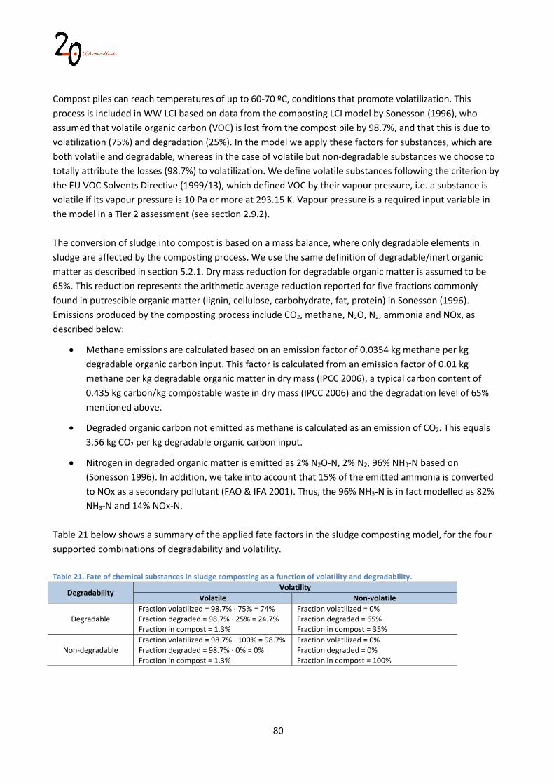
80

Compost piles can reach temperatures of up to 60-70 ºC, conditions that promote volatilization. This process is included in WW LCI based on data from the composting LCI model by Sonesson (1996), who assumed that volatile organic carbon (VOC) is lost from the compost pile by 98.7%, and that this is due to volatilization (75%) and degradation (25%). In the model we apply these factors for substances, which are both volatile and degradable, whereas in the case of volatile but non-degradable substances we choose to totally attribute the losses (98.7%) to volatilization. We define volatile substances following the criterion by the EU VOC Solvents Directive (1999/13), which defined VOC by their vapour pressure, i.e. a substance is volatile if its vapour pressure is 10 Pa or more at 293.15 K. Vapour pressure is a required input variable in the model in a Tier 2 assessment (see section 2.9.2). The conversion of sludge into compost is based on a mass balance, where only degradable elements in sludge are affected by the composting process. We use the same definition of degradable/inert organic matter as described in section 5.2.1. Dry mass reduction for degradable organic matter is assumed to be 65%. This reduction represents the arithmetic average reduction reported for five fractions commonly found in putrescible organic matter (lignin, cellulose, carbohydrate, fat, protein) in Sonesson (1996). Emissions produced by the composting process include CO2, methane, N2O, N2, ammonia and NOx, as described below:

Methane emissions are calculated based on an emission factor of 0.0354 kg methane per kg degradable organic carbon input. This factor is calculated from an emission factor of 0.01 kg methane per kg degradable organic matter in dry mass (IPCC 2006), a typical carbon content of 0.435 kg carbon/kg compostable waste in dry mass (IPCC 2006) and the degradation level of 65% mentioned above.

Degraded organic carbon not emitted as methane is calculated as an emission of CO2. This equals 3.56 kg CO2 per kg degradable organic carbon input.

Nitrogen in degraded organic matter is emitted as 2% N2O-N, 2% N2, 96% NH3-N based on (Sonesson 1996). In addition, we take into account that 15% of the emitted ammonia is converted to NOx as a secondary pollutant (FAO & IFA 2001). Thus, the 96% NH3-N is in fact modelled as 82% NH3-N and 14% NOx-N.

Table 21 below shows a summary of the applied fate factors in the sludge composting model, for the four supported combinations of degradability and volatility. Table 21. Fate of chemical substances in sludge composting as a function of volatility and degradability.

Degradability Volatility

Volatile Non-volatile

Degradable Fraction volatilized = 98.7% · 75% = 74% Fraction degraded = 98.7% · 25% = 24.7% Fraction in compost = 1.3%

Fraction volatilized = 0% Fraction degraded = 65% Fraction in compost = 35%

Non-degradable Fraction volatilized = 98.7% · 100% = 98.7% Fraction degraded = 98.7% · 0% = 0% Fraction in compost = 1.3%

Fraction volatilized = 0% Fraction degraded = 0% Fraction in compost = 100%

81

A water balance is also established. Based on typical values for moisture content in input sludge of 28% (Poulsen and Hansen 2003), wet mass reduction during composting of 57% (Poulsen and Hansen 2003) as well as moisture content in compost of 50% (Sonesson 1996), a fixed water evaporation rate of 70% of the water input is applied to all sludge components. For mass balance purposes, the consumption of atmospheric oxygen during composting is calculated, based on the stoichiometric requirements to form CO2 from carbon in degradable organic matter (0.727 kg Oxygen per kg CO2). The amount of final compost obtained in wet weight (Compostwet) is calculated with Equation 66: Compostwet = (sludgewet + O2) - (H2O + CO2 + CH4 + N2 + N2O + NH3 + NOx) Equation 66. Calculation of compost production. Based on the initial composition of sludge entering the composting plant and the detailed mass balance, the composition of the resulting compost is obtained, including the fraction (if any) of original substances discharged in wastewater, still remaining in the compost. This composition is used as input for the calculations on application of compost in agriculture, which follows the same principles as sludge application in agriculture, described in section 5.2.7. 5.2.7 Application of sludge and compost in agriculture The inventory for application of sludge and compost obtained from the latter as fertilizers in agriculture includes the following:

Emissions to air, soil and water as a result of sludge and compost application. Substitution of mineral N and P fertilizers

Direct emissions to soil are obtained from the sludge or compost composition and include the following:

Emission to soil of any remaining fraction of the substances initially present in wastewater, if partitioned to sludge in WWTPs.

Emission to soil of polyelectrolyte used as coagulant and sludge conditioner.

Emission to soil as chloride of any chlorine in sludge.

Emission to soil as sulfate of any sulfur in sludge.

Emission to soil of iron contained in iron hydroxides or iron phosphate.

Emission to soil of water in dewatered sludge. To reflect the process of sludge and compost mineralization, the following emissions to air are calculated: CO2, NH3, NOx (as NO2), and N2O. Emissions of NO3 from leaching to groundwater are also included, while no losses of phosphorus are considered either to surface water or groundwater. The calculation of these emissions is described below. CO2 emissions from sludge mineralization are calculated stoichiometrically, based on the amount of degradable carbon (the latter as defined in section 5.2.1) contained in the sludge, which is assumed to be transformed completely to CO2.

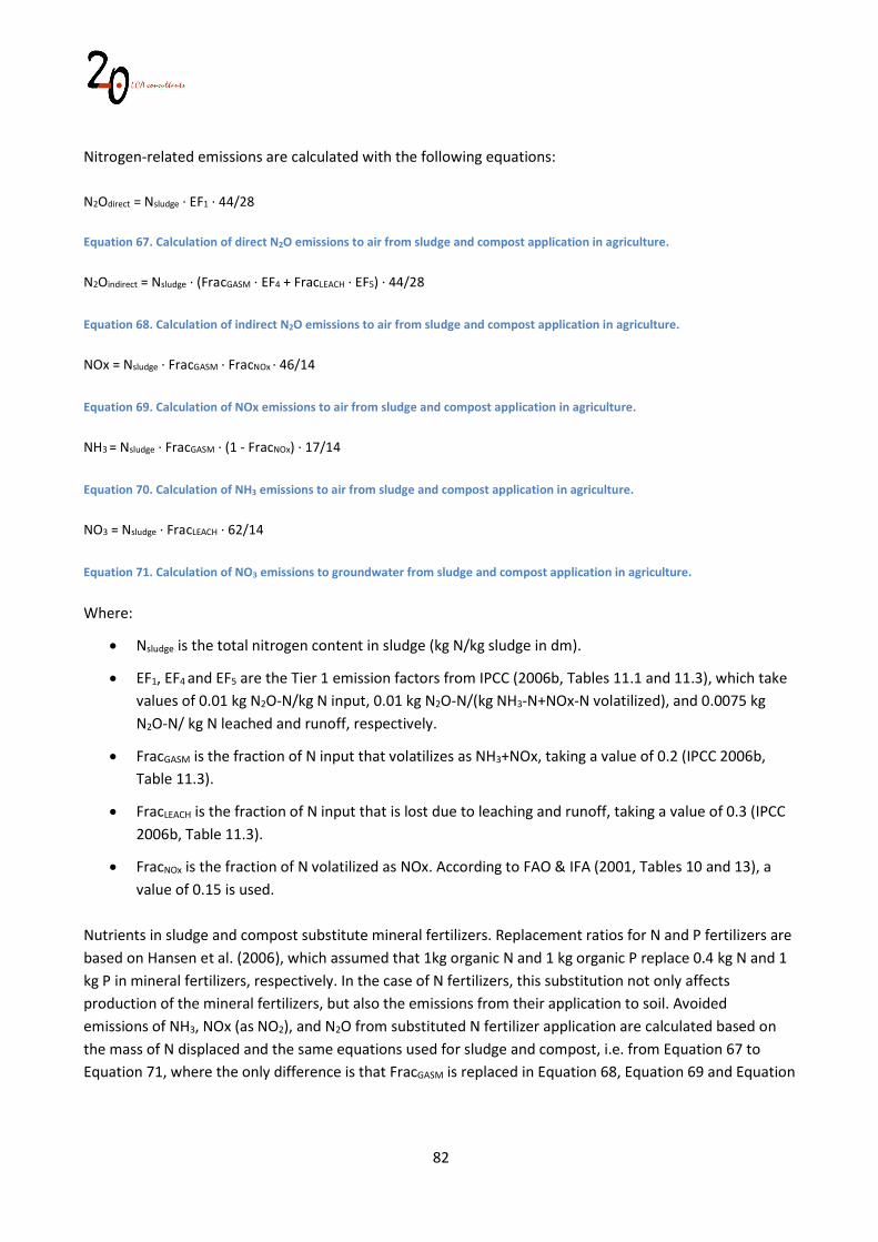
82

Nitrogen-related emissions are calculated with the following equations: N2Odirect = Nsludge · EF1 · 44/28 Equation 67. Calculation of direct N2O emissions to air from sludge and compost application in agriculture. N2Oindirect = Nsludge · (FracGASM · EF4 + FracLEACH · EF5) · 44/28 Equation 68. Calculation of indirect N2O emissions to air from sludge and compost application in agriculture. NOx = Nsludge · FracGASM · FracNOx · 46/14 Equation 69. Calculation of NOx emissions to air from sludge and compost application in agriculture. NH3 = Nsludge · FracGASM · (1 - FracNOx) · 17/14 Equation 70. Calculation of NH3 emissions to air from sludge and compost application in agriculture. NO3 = Nsludge · FracLEACH · 62/14 Equation 71. Calculation of NO3 emissions to groundwater from sludge and compost application in agriculture. Where:

Nsludge is the total nitrogen content in sludge (kg N/kg sludge in dm).

EF1, EF4 and EF5 are the Tier 1 emission factors from IPCC (2006b, Tables 11.1 and 11.3), which take values of 0.01 kg N2O-N/kg N input, 0.01 kg N2O-N/(kg NH3-N+NOx-N volatilized), and 0.0075 kg N2O-N/ kg N leached and runoff, respectively.

FracGASM is the fraction of N input that volatilizes as NH3+NOx, taking a value of 0.2 (IPCC 2006b, Table 11.3).

FracLEACH is the fraction of N input that is lost due to leaching and runoff, taking a value of 0.3 (IPCC 2006b, Table 11.3).

FracNOx is the fraction of N volatilized as NOx. According to FAO & IFA (2001, Tables 10 and 13), a value of 0.15 is used.

Nutrients in sludge and compost substitute mineral fertilizers. Replacement ratios for N and P fertilizers are based on Hansen et al. (2006), which assumed that 1kg organic N and 1 kg organic P replace 0.4 kg N and 1 kg P in mineral fertilizers, respectively. In the case of N fertilizers, this substitution not only affects production of the mineral fertilizers, but also the emissions from their application to soil. Avoided emissions of NH3, NOx (as NO2), and N2O from substituted N fertilizer application are calculated based on the mass of N displaced and the same equations used for sludge and compost, i.e. from Equation 67 to Equation 71, where the only difference is that FracGASM is replaced in Equation 68, Equation 69 and Equation

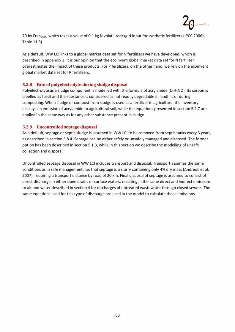
83

70 by FracGASF, which takes a value of 0.1 kg N volatilized/kg N input for synthetic fertilizers (IPCC 2006b, Table 11.3). As a default, WW LCI links to a global market data set for N fertilizers we have developed, which is described in appendix 3. It is our opinion that the ecoinvent global market data set for N fertilizer overestimates the impact of these products. For P fertilizers, on the other hand, we rely on the ecoinvent global market data set for P fertilizers. 5.2.8 Fate of polyelectrolyte during sludge disposal Polyelectrolyte as a sludge component is modelled with the formula of acrylamide (C3H5NO). Its carbon is labelled as fossil and the substance is considered as not readily degradable in landfills or during composting. When sludge or compost from sludge is used as a fertilizer in agriculture, the inventory displays an emission of acrylamide to agricultural soil, while the equations presented in section 5.2.7 are applied in the same way as for any other substance present in sludge. 5.2.9 Uncontrolled septage disposal As a default, septage or septic sludge is assumed in WW LCI to be removed from septic tanks every 3 years, as described in section 3.8.4. Septage can be either safely or unsafely managed and disposed. The former option has been described in section 5.1.3, while in this section we describe the modelling of unsafe collection and disposal. Uncontrolled septage disposal in WW LCI includes transport and disposal. Transport assumes the same conditions as in safe management, i.e. that septage is a slurry containing only 4% dry mass (Andreoli et al. 2007), requiring a transport distance by road of 20 km. Final disposal of septage is assumed to consist of direct discharge in either open drains or surface waters, resulting in the same direct and indirect emissions to air and water described in section 4 for discharges of untreated wastewater through closed sewers. The same equations used for this type of discharge are used in the model to calculate those emissions.

84

6 Energy balance in WWTPs

This section addresses the balances of electricity and thermal energy in centralized WWTPs. The term balance is deliberately used, given that WWTPs may at the same time demand energy to operate, but also produce energy thanks to CHP units using biogas. The net (electric or thermal) energy use, then, is the difference between these two, as shown in Equation 72. When a negative energy use results, this surplus is modelled by substitution of the corresponding type and amount of energy. This equation is applied to each substance discharged in wastewater and treated in WWTPs. Energy use = Energy demand - Energy production Equation 72. Energy balance at WWTPs. The processes described in this section apply to WWTPs with either primary, secondary or tertiary treatment, with the exception of stabilization ponds, as in the model this type of plant is assumed not to require any energy input.

6.1 Electricity balance In WW LCI, the electricity balance for a given substance treated in a WWTP depends both on substance-specific conditions as well as on scenario conditions. Substance-specific conditions determine whether the substance degrades or not, if it is partitioned to sludge, etc., with each of these processes being attributed specific electricity consumption factors. Scenario conditions include the type of plant where the substance is treated (primary, secondary, tertiary treatment), if the plant has anaerobic digestion of sludge, and last but not least, the plant size, with bigger plants being attributed lower electricity demand on a per m3 basis, as described below. 6.1.1 Electricity demand and WWTP size It is well known that electricity demand in WWTPs is influenced by size, where the latter can be expressed as the plant’s daily flow in m3/d. Bigger plants show generally lower consumption on a per m3 or person-equivalent (PE) basis (CUAS 2015; Trapote et al. 2014). According to CUAS (2015) this is due to economies of scale in larger systems, leading to larger but more efficient equipment, better performing automation and regulation, and also to more and better-trained staff operating the plants. In WW LCI we address this by adding a so-called ‘scale factor’, which is a multiplier factor that increases the electricity demand of the plant as its size decreases. We established the relationship between kWh/m3 and WWTP size using two studies in the US (Stillwell et al. 2010) and Spain (Albadalejo et al. 2017). Figure 13 below plots the data obtained from these studies, together with power regressions. Data from the two studies were used as they cover WWTPs of different sizes, with the Spanish study reaching to smaller sizes while the US study reaches to bigger sizes. In WW LCI we take a WWTP treating 2 million m3/d as reference, i.e. the size beyond which higher efficiency is not considered. The regressions in Figure 13 predict that such a plant has an electricity demand of 0.23 kWh/m3 (based on ES data) and 0.30 kWh/m3 (based on US data). In the model we take the arithmetic average of these two, namely 0.27 kWh/m3.

85

Figure 13. Electricity consumption in WWTPs (kWh/m3) as a function of daily wastewater flow (m3/d) in United States and Spain. Underlying data from Stillwell et al. (2010) and Albadalejo et al. (2017). In Figure 14 below the energy demand of WWTPs as predicted by the two regressions calculated in Figure 13 is divided by the demand of the reference plant (0.27 kWh/m3). We call this ratio the ‘scale factor’. The reference WWTP is thus attributed a scale factor of 1, whereas smaller WWTPs have a scale factor above 1. It can be seen that both studies lead to very similar scale factors. For example, a WWTP treating 500,000 m3/d gets a scale factor of 1.20 using the US regression and 1.22 using the Spanish study regression. We finally merge the scale factors of the two studies by means of a polynomic regression, resulting in Equation 73: SF = 7.5316x-0.139

Equation 73. Calculation of the scale factor for electricity demand in WWTPs. Where SF is the scale factor (dimensionless) and x is the plant’s daily wastewater flow in m3/day.

Figure 14. Derivation of a scale factor relating WWTP size with electricity consumption per m3, based on the data from Figure 13. 6.1.2 Subdivision of electricity demand In WW LCI, electricity demand in WWTPs is subdivided into a set of activities, to which specific electricity consumption factors are attributed:

86

Aeration: electricity consumed by blowers to supply oxygen to the biological treatment basin. This is attributed to wastewater components based on their total oxygen consumption, which is determined stoichiometrically by means of Equation 6 and Equation 9. This also includes oxygen to form N2O (see section 3.3.6) and to oxidize organic sulfur and phosphorus to sulfate and orthophosphate, respectively (see section 3.3.5).

Sludge treatment: electricity consumed by primary and secondary settling tanks, anaerobic digestion (if available), thickening and dewatering. This is attributed to wastewater components based on the amount of raw sludge they produce, as dry mass.

Miscellaneous: this includes building energy consumption (offices, labs, etc.) as well as pre-treatment and pumping of wastewater inside the plant. This miscellaneous demand is attributed to the wastewater components on a mass basis. All wastewater components are attributed the same demand related to these activities.

The above-mentioned three electricity demand categories are further specified according to the treatment level in the WWTP. For example, a WWTP with primary treatment does not demand electricity for aeration. The electricity demand factors used are shown in Table 22, for the reference WWTP treating 2 million m3/day. Miscellaneous demand factors were derived from a distribution in percentages of electricity demand in different activities by a WWTP treating 100 megagallon/day or 378,541 m3/day (Stillwell et al. 2010). These percentages were converted into kWh/m3 considering the electricity demand for the reference WWTP of 0.27 kWh/m3. The electricity demand for sludge treatment originates in the same source (Stillwell et al. 2010). In this case we assumed that 1 m3 wastewater produces 0.35 kg raw sludge, based on 0.06-0.08 kg solids/PE in activated sludge plants (Andreoli et al. 2007) and a wastewater volume of 0.2 m3/PE/d (Henze and Comeau 2008). Finally, the electricity demand for aeration is taken from Von Sperling (2007a) as an average from different aeration methods (diffused air, mechanical aeration). Table 22. Electricity demand factors considered in WW LCI for a reference WWTP treating 2 million m3/d.

Operation Unit WWTP with

primary treatment

WWTP with secondary treatment

WWTP with tertiary

treatment Miscellaneous kWh/m3 0.027 0.027 0.028 Sludge treatment, no anaerobic digestion kWh/kg solids 0.086 0.112 0.181 Sludge treatment, with anaerobic digestion kWh/kg solids 0.162 0.188 0.258 Aeration kWh/kg O2 0 0.714 0.714 The electricity demand factors in Table 22 refer to a WWTP treating 2 million m3/day, while for smaller plants the scale factor needs to be applied. For example, a WWTP with secondary treatment and anaerobic digestion of sludge treating 500,000 m3/d has a scale factor of 1.21 according to Equation 73. Its electricity demand for sludge treatment is thus 1.21*0.188 = 0.227 kWh/kg solids. Overall, the electricity demand for a given substance treated in a WWTP (Delec), expressed in kWh/kg substance, is calculated with Equation 74: Delec = SF · (Miscelec + Sludgeelec · Sludgedm + Aerationelec · O2) Equation 74. Calculation of electricity demand in WWTPs.

87

Where:

SF is the scale factor, calculated with Equation 73.

Miscelec is the electricity demand for miscellaneous purposes, as shown in Table 22, expressed in kWh/kg substance.

Sludgeelec is the electricity demand for sludge treatment, as shown in Table 22, expressed in kWh/kg sludge in dry mass.

Sludgedm is the sludge production by the substance, in kg dry mass/kg substance, including all the components mentioned in section 5.2.1.

Aerationelec is the electricity demand for aeration, as shown in Table 22, expressed in kWh/kg O2.

O2 is the oxygen consumed for aeration, expressed as kg O2/kg substance. 6.1.3 Electricity production Electricity production is considered only for WWTPs with anaerobic digestion of sludge and a CHP unit, where biogas is converted to heat and electricity. Electricity and heat production are therefore only attributed to substances expected to degrade in anaerobic digesters, as defined in section 5.1.1. Electricity production (Prodelec) for a given substance treated in a WWTP, expressed in kWh/kg substance is calculated with Equation 75:

Prodelec = (CH4 prod - CH4 esc) · LHVCH4 · CHPeff-elec

3.6 Equation 75. Calculation of electricity production in WWTPs. Where:

CH4 prod is the production of methane during anaerobic digestion of sludge, expressed in kg methane per kg substance, as described in section 5.1.1.

CH4 esc is non-combusted methane escaping to the atmosphere, expressed in kg methane per kg substance, as described in section 5.1.2.

LHVCH4 is the low heating value of methane, taken as 50 MJ/kg.

CHPeff-elec is the electric efficiency by the CHP unit. As a default, this takes a value of 26.8%, as the average from five technologies described in Wason (2006).

Table 23 shows an example of an electricity balance, for the substances ibuprofen and zeolite A, based on substance-specific data from Kalbar et al. (2018) and Muñoz et al. (2017). These substances are compared under two scenarios for a WWTP with secondary treatment (activated sludge): a plant treating 10,000 m3/d with no anaerobic digestion of sludge, and a bigger plant treating 100,000 m3/d that applies anaerobic digestion of sludge and uses biogas in a CHP unit. Ibuprofen is a degradable compound, while zeolites are inert, for this reason ibuprofen registers an electricity demand for aeration, to supply oxygen for biological degradation, while zeolite A only demands electricity for sludge processing (90% of the substance is

88

assumed to partition to sludge). In the bigger plant it can be seen that electricity demand for aeration decreases, due to the size effect, as described in section 6.1.1. Demand for sludge processing, however, increases, given that this plant requires additional electricity to run the anaerobic digestion process. Finally, the implementation of the CHP unit allows the bigger plant to recover part of the energy in ibuprofen’s sludge as electricity, offsetting part of the overall demand. This, however, does not affect zeolite A, as its sludge is inorganic and does not produce any biogas. Table 23. Example of electricity balance for ibuprofen and zeolite A in a hypothetical WWTP with secondary treatment by activated sludge, depending on plant size and implementation of anaerobic digestion and CHP. Figures in kWh per kg substance at the WWTP inlet.

WWTP settings Substance Aerationelec (kWh/kg)

Sludgeelec (kWh/kg)

Miscelec (kWh/kg)

Prodelec

(kWh/kg) Net demand

(kWh/kg) 10,000 m3/d, no anaerobic digestion

Ibuprofen 1.73 0.12 5.7E-05 0 1.85 Zeolite 0 0.21 5.7E-05 0 0.21

100,000 m3/d, anaerobic digestion + CHP

Ibuprofen 1.25 0.15 4.2E-05 0.35 1.06 Zeolite 0 0.26 4.2E-05 0 0.26

6.2 Heat balance As in the electricity balance, the heat balance for a given substance treated in a WWTP depends both on substance-specific conditions as well as on scenario conditions. Substance-specific conditions determine, for example, whether or not a substance degrades during anaerobic digestion. Scenario conditions include the type of plant where the substance is treated (primary, secondary, tertiary treatment) and most notably, if the plant has anaerobic digestion of sludge. However, as opposed to electricity demand, in WW LCI plant size has no effect on the heat balance. A heat balance is calculated for each substance treated in a WWTP, taking into consideration the following:

Heat demand for sludge digestion, calculated considering local climatic conditions (ambient temperature).

Heat demand for miscellaneous purposes (e.g. heating of buildings).

Heat production is calculated from the amount of methane produced during anaerobic digestion and the heat recovery efficiency, depending on whether biogas is combusted in a boiler or in a CHP unit.

Based on these three terms, the balance leads to either a net heat surplus or a net heat demand. In both cases, the model calculates, based on the local climatic conditions, whether the marginal source of heat either substituted or consumed is biogas, natural gas or a combination of the two. In section 6.2.1 below we describe the heat balance model, at the level of the WWTP as a whole, while section 6.2.2 describes the calculation of the marginal source of heat. Finally, section 6.2.3 establishes how the data at the WWTP level is used to derive a substance-specific heat balance, illustrating this with an example.

89

6.2.1 Heat balance model Heat demand by anaerobic digestion is calculated based on data and equations provided in Turovskiy and Mathai (2006) for a WWTP treating 37,800 m3 wastewater/day and producing 5,443 kg primary sludge and 2,722 kg activated sludge per day, which are treated in two mesophilic digesters with 15 m diameter, where a hydraulic residence time of 20 days is assumed, based on a range of 18 to 25 days (Andreoli et al. 2007). The total volume of the digester (as the sum of the two units) is 3,499 m3. The underlying geometrical data by Turovskiy and Mathai (2006) allow us to calculate for each digester, in m2, the floor area (180 m2), wall area (561 m2), and roof area (177 m2). The total heat demand by the WWTP, in MJ/day, including anaerobic digestion and other miscellaneous uses, is calculated with Equation 76:

Dheat-AD = L + S 0.9

Equation 76. Calculation of the thermal energy demand by the WWTP, in MJ/day. Where L is the heat demand to offset the sum of heat losses through the digester’s wall, floor and roof, while S is the heat required to increase the sludge temperature from ambient conditions to the 35ºC maintained in the digester. The 0.9 factor is meant to account for additional heating demand in the WWTP, i.e. the miscellaneous component of heat demand by the WWTP. The latter is quantified at 10% of the total heating demand of the WWTP as in Doka (2007). The Losses (L) for each one of the digester surfaces are calculated with Equation 77:

L = U · A · (35 – T) 1000 · 24 · 3.6

Equation 77. Calculation of heat losses by the anaerobic digester through either wall, floor or roof. Where U is the heat transfer coefficient (W/m2/ºC) for either floor, wall or roof, A is the total area of each surface and T is the temperature (ºC) of either air (for losses through wall and roof) or soil (for losses through floor). Values for U are taken from Foley et al. (2010) as 5, 1.7 and 2 W/m2/ºC for wall, floor and roof, respectively. These values are assumed to be constant across countries. S, in MJ/day, is calculated with Equation 78: S = Q · Cp · (35 – T) Equation 78. Calculation of heat demand to increase sludge temperature from ambient temperature to 35 ºC. Where Q is the sludge flow in m3/day, Cp is the heat capacity of sludge in MJ/m3/ºC and T is the sludge temperature (ºC). Q is calculated as 87.5 m3/day per digester and Cp for sludge is assimilated to that of water, i.e. 4.2 MJ/m3/ºC. As it can be seen, the formulae for L and S depend on temperatures of three media: air, soil and sludge. In WW LCI these three temperatures are site-specific, but also time-specific. Each country is attributed its own average temperature profile, varying on a monthly basis, from January to December. Thus, L and S in WW

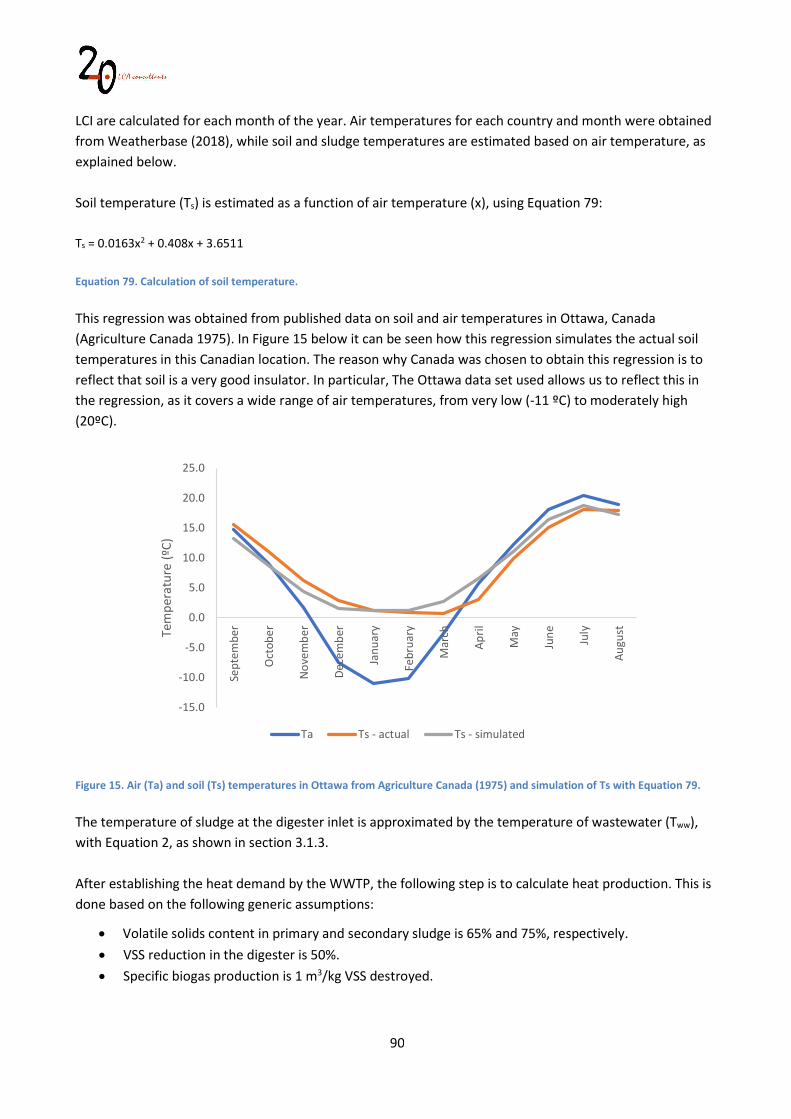
90

LCI are calculated for each month of the year. Air temperatures for each country and month were obtained from Weatherbase (2018), while soil and sludge temperatures are estimated based on air temperature, as explained below. Soil temperature (Ts) is estimated as a function of air temperature (x), using Equation 79: Ts = 0.0163x2 + 0.408x + 3.6511 Equation 79. Calculation of soil temperature. This regression was obtained from published data on soil and air temperatures in Ottawa, Canada (Agriculture Canada 1975). In Figure 15 below it can be seen how this regression simulates the actual soil temperatures in this Canadian location. The reason why Canada was chosen to obtain this regression is to reflect that soil is a very good insulator. In particular, The Ottawa data set used allows us to reflect this in the regression, as it covers a wide range of air temperatures, from very low (-11 ºC) to moderately high (20ºC).

Figure 15. Air (Ta) and soil (Ts) temperatures in Ottawa from Agriculture Canada (1975) and simulation of Ts with Equation 79. The temperature of sludge at the digester inlet is approximated by the temperature of wastewater (Tww), with Equation 2, as shown in section 3.1.3. After establishing the heat demand by the WWTP, the following step is to calculate heat production. This is done based on the following generic assumptions:

Volatile solids content in primary and secondary sludge is 65% and 75%, respectively. VSS reduction in the digester is 50%. Specific biogas production is 1 m3/kg VSS destroyed.

-15.0

-10.0

-5.0

0.0

5.0

10.0

15.0

20.0

25.0

Sept

embe

r

Oct

ober

Nov

embe

r

Dec

embe

r

Janu

ary

Febr

uary

Mar

ch

April

May

June July

Augu

stTem

pera

ture

(ºC)

Ta Ts - actual Ts - simulated

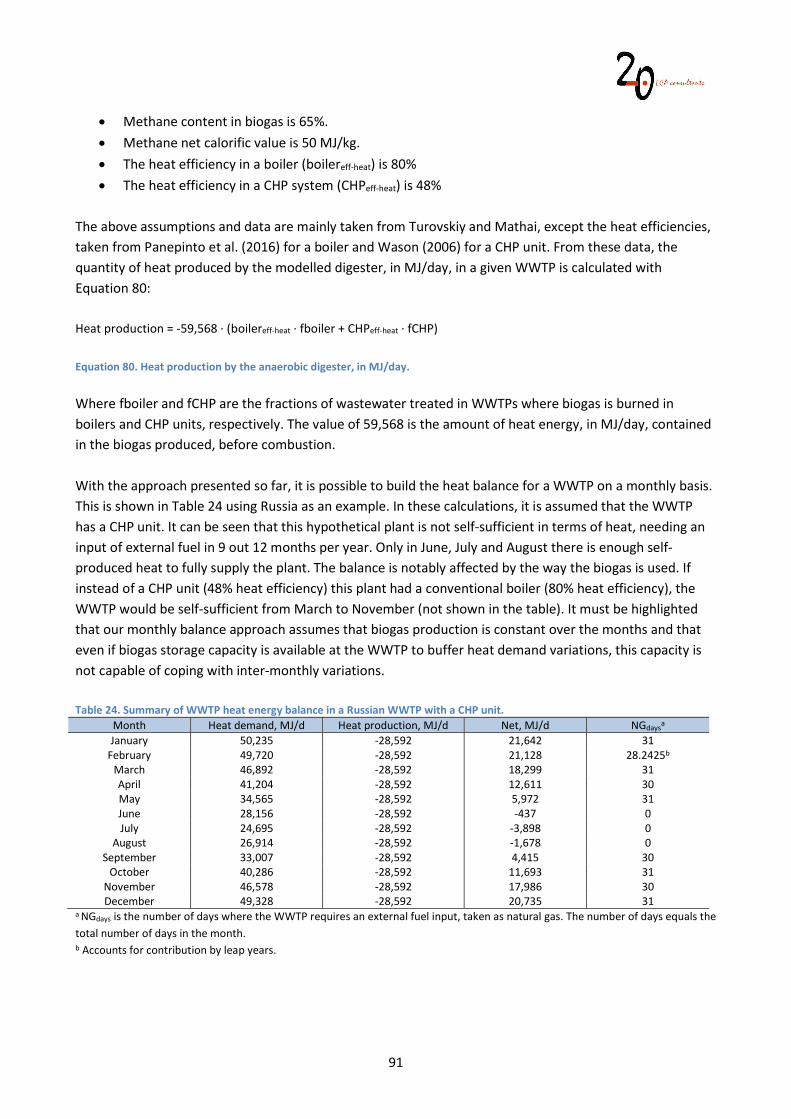
91

Methane content in biogas is 65%. Methane net calorific value is 50 MJ/kg. The heat efficiency in a boiler (boilereff-heat) is 80% The heat efficiency in a CHP system (CHPeff-heat) is 48%

The above assumptions and data are mainly taken from Turovskiy and Mathai, except the heat efficiencies, taken from Panepinto et al. (2016) for a boiler and Wason (2006) for a CHP unit. From these data, the quantity of heat produced by the modelled digester, in MJ/day, in a given WWTP is calculated with Equation 80: Heat production = -59,568 · (boilereff-heat · fboiler + CHPeff-heat · fCHP) Equation 80. Heat production by the anaerobic digester, in MJ/day. Where fboiler and fCHP are the fractions of wastewater treated in WWTPs where biogas is burned in boilers and CHP units, respectively. The value of 59,568 is the amount of heat energy, in MJ/day, contained in the biogas produced, before combustion. With the approach presented so far, it is possible to build the heat balance for a WWTP on a monthly basis. This is shown in Table 24 using Russia as an example. In these calculations, it is assumed that the WWTP has a CHP unit. It can be seen that this hypothetical plant is not self-sufficient in terms of heat, needing an input of external fuel in 9 out 12 months per year. Only in June, July and August there is enough self-produced heat to fully supply the plant. The balance is notably affected by the way the biogas is used. If instead of a CHP unit (48% heat efficiency) this plant had a conventional boiler (80% heat efficiency), the WWTP would be self-sufficient from March to November (not shown in the table). It must be highlighted that our monthly balance approach assumes that biogas production is constant over the months and that even if biogas storage capacity is available at the WWTP to buffer heat demand variations, this capacity is not capable of coping with inter-monthly variations. Table 24. Summary of WWTP heat energy balance in a Russian WWTP with a CHP unit.

Month Heat demand, MJ/d Heat production, MJ/d Net, MJ/d NGdaysa January 50,235 -28,592 21,642 31

February 49,720 -28,592 21,128 28.2425b March 46,892 -28,592 18,299 31 April 41,204 -28,592 12,611 30 May 34,565 -28,592 5,972 31 June 28,156 -28,592 -437 0 July 24,695 -28,592 -3,898 0

August 26,914 -28,592 -1,678 0 September 33,007 -28,592 4,415 30

October 40,286 -28,592 11,693 31 November 46,578 -28,592 17,986 30 December 49,328 -28,592 20,735 31

a NGdays is the number of days where the WWTP requires an external fuel input, taken as natural gas. The number of days equals the total number of days in the month. b Accounts for contribution by leap years.

92

The benefit of this monthly approach is that it allows us to obtain a more accurate picture of the heat balance when compared to a single average annual value. Based on the numbers in Table 24, it can be calculated that this plant requires 14.3 TJ per year, while it only produces 10.4 TJ per year. This points to an annual heat deficit of 3.9 TJ. On the other hand, the monthly balance gives us a higher resolution, where we see that in summer the plant is in fact self-sufficient. This has implications in terms of determining the marginal, i.e. the affected source of energy when we calculate substance-specific inventories leading to a net heat demand or surplus. The determination of this marginal heat mix is described in the next section. Obviously, there is no reason why one should stop at the monthly resolution in the heat balance, as the same balance could be determined on a daily basis. This could maybe lead us to identify some further days in the year where the plant is also self-sufficient, while this is lost at the monthly resolution. However, collecting and processing 365 temperatures per country would be excessive for the purposes of WW LCI. Also, as we shorten the time frame, i.e. days instead of months, we are more likely to incur in errors if the plants have some kind of biogas storage capacity allowing them to alleviate demand variations. 6.2.2 Marginal heat mix The heat balance described in the previous section leads to either a net heat surplus or a net heat demand in the WWTP. The marginal heat mix reflects the expected source of energy that will provide this additional demand (in case there is a net heat demand) or that will be substituted (in case there is a net heat surplus). It is called a ‘mix’ because it is contributed by two possible sources for heat production: biogas produced by the WWTP itself, or an external fuel, the latter modelled as natural gas. The percentages of natural gas and biogas in this mix are calculated with Equation 81 and Equation 82:

%NG = NGdays

365.2425 Equation 81. Calculation of the natural gas component in the marginal heat mix. %Biogas = 100% - %NG Equation 82. Calculation of the biogas component in the marginal heat mix. Where NGdays is the total number of days in an average year where the plant requires an external input of fuel. In the example of Russia (Table 24) this sum equals 273.2425 days, out of 365.2425 days. In this way, the marginal heat mix for the Russian WWTP is 75% natural gas and 25% biogas. 6.2.3 Substance-specific heat balance In the previous sections we have described the heat balance for a WWTP as a whole, expressed in MJ/day, as well as its marginal heat mix. The next step is to establish how this information is used in WW LCI on a wastewater component basis. i.e. per kg of a substance discharged in wastewater and treated in such a WWTP. The daily heat balance is used to obtain the following data:

Heat demand for treating sludge in anaerobic digestion, in MJ/kg dry mass sent to digestion (Equation 83).

Heat demand for miscellaneous purposes, in MJ/kg component treated in the WWTP (Equation 84).

93

Heat production from combustion of biogas, in MJ/kg component treated in the WWTP (Equation 85).

The country-specific heat demand for treating sludge in anaerobic digestion, in MJ/kg dry mass sent to digestion (Heatsludge), is calculated with Equation 83:

Heatsludge = (L + S) · 0.9

(5,443 + 2,722) Equation 83. Heat demand by the anaerobic digester, in MJ/kg sludge dry mass. Where 5,443 and 2,722 are the amounts, in kg dry mass, of primary and secondary sludge fed to the digester on a daily basis, as described in section 6.2.1. Heatsludge is calculated on a monthly basis and an annual weighted average is derived from the 12 months. The numerator is multiplied by 0.9 as in our model it is assumed that 90% of the heat energy demand in the WWTP is associated with the digester, as described in section 6.2.1. In the example of Russia (Table 24), the annual weighted average value for Heatsludge is 4.32 MJ/kg sludge dry mass. Thus, in WW LCI, a wastewater component producing 1kg sludge in a Russian WWTP with anaerobic digestion is attributed this heat demand. The country-specific heat demand for miscellaneous purposes, in MJ/kg component at the WWTP inlet, is calculated with Equation 84:

Heatmisc = (L + S) · 0.1 37,800,000

Equation 84. Heat demand for miscellaneous purposes in a WWTP, in MJ/kg substance at the WWTP inlet. Where 37,800,000 is the volume of wastewater (in L or kg) treated daily by the WWTP considered in the anaerobic digestion model. As described in section 6.2.1, these miscellaneous purposes are assumed to demand 10% of the total heat used by the WWTP, whereby the 0.1 factor in the equation. In the example of Russia (Table 24), we obtain a value of 1.04E-04 MJ/kg. Heatmisc is a generic heat demand in the WWTP and as such it is attributed to all wastewater components entering the plant, on a mass basis. In those cases where the WWTP does not have anaerobic digestion, this parameter is calculated in the same way. Heat production (Prodheat) is only attributed to substances expected to degrade in anaerobic digesters, as defined in section 5.1.1. This is expressed in MJ/kg substance at the WWTP inlet, and calculated with Equation 85: Prodheat = (CH4 prod - CH4 esc) · LHVCH4 · (boilereff-heat · fboiler + CHPeff-heat · fCHP) Equation 85. Calculation of heat production in WWTPs, in MJ/kg substance at the WWTP inlet. The net demand or surplus of an external fuel, namely natural gas (NG), is finally calculated with Equation 86, as MJ/kg substance at the WWTP inlet:

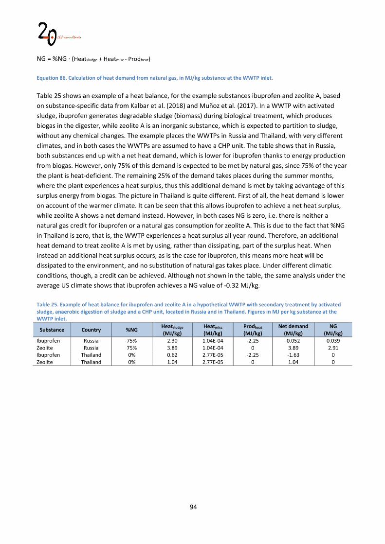
94

NG = %NG · (Heatsludge + Heatmisc - Prodheat) Equation 86. Calculation of heat demand from natural gas, in MJ/kg substance at the WWTP inlet. Table 25 shows an example of a heat balance, for the example substances ibuprofen and zeolite A, based on substance-specific data from Kalbar et al. (2018) and Muñoz et al. (2017). In a WWTP with activated sludge, ibuprofen generates degradable sludge (biomass) during biological treatment, which produces biogas in the digester, while zeolite A is an inorganic substance, which is expected to partition to sludge, without any chemical changes. The example places the WWTPs in Russia and Thailand, with very different climates, and in both cases the WWTPs are assumed to have a CHP unit. The table shows that in Russia, both substances end up with a net heat demand, which is lower for ibuprofen thanks to energy production from biogas. However, only 75% of this demand is expected to be met by natural gas, since 75% of the year the plant is heat-deficient. The remaining 25% of the demand takes places during the summer months, where the plant experiences a heat surplus, thus this additional demand is met by taking advantage of this surplus energy from biogas. The picture in Thailand is quite different. First of all, the heat demand is lower on account of the warmer climate. It can be seen that this allows ibuprofen to achieve a net heat surplus, while zeolite A shows a net demand instead. However, in both cases NG is zero, i.e. there is neither a natural gas credit for ibuprofen or a natural gas consumption for zeolite A. This is due to the fact that %NG in Thailand is zero, that is, the WWTP experiences a heat surplus all year round. Therefore, an additional heat demand to treat zeolite A is met by using, rather than dissipating, part of the surplus heat. When instead an additional heat surplus occurs, as is the case for ibuprofen, this means more heat will be dissipated to the environment, and no substitution of natural gas takes place. Under different climatic conditions, though, a credit can be achieved. Although not shown in the table, the same analysis under the average US climate shows that ibuprofen achieves a NG value of -0.32 MJ/kg. Table 25. Example of heat balance for ibuprofen and zeolite A in a hypothetical WWTP with secondary treatment by activated sludge, anaerobic digestion of sludge and a CHP unit, located in Russia and in Thailand. Figures in MJ per kg substance at the WWTP inlet.

Substance Country %NG Heatsludge (MJ/kg)

Heatmisc

(MJ/kg) Prodheat

(MJ/kg) Net demand

(MJ/kg) NG

(MJ/kg) Ibuprofen Russia 75% 2.30 1.04E-04 -2.25 0.052 0.039 Zeolite Russia 75% 3.89 1.04E-04 0 3.89 2.91 Ibuprofen Thailand 0% 0.62 2.77E-05 -2.25 -1.63 0 Zeolite Thailand 0% 1.04 2.77E-05 0 1.04 0

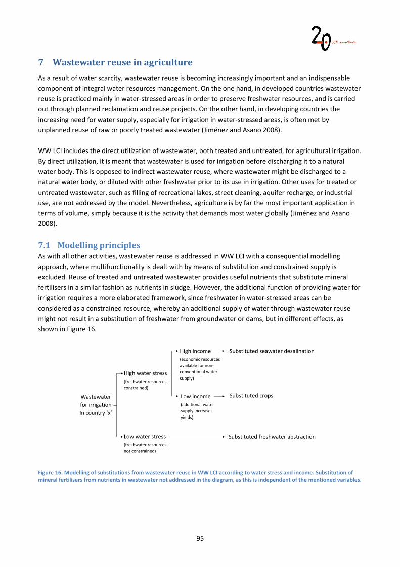
95

7 Wastewater reuse in agriculture

As a result of water scarcity, wastewater reuse is becoming increasingly important and an indispensable component of integral water resources management. On the one hand, in developed countries wastewater reuse is practiced mainly in water-stressed areas in order to preserve freshwater resources, and is carried out through planned reclamation and reuse projects. On the other hand, in developing countries the increasing need for water supply, especially for irrigation in water-stressed areas, is often met by unplanned reuse of raw or poorly treated wastewater (Jiménez and Asano 2008). WW LCI includes the direct utilization of wastewater, both treated and untreated, for agricultural irrigation. By direct utilization, it is meant that wastewater is used for irrigation before discharging it to a natural water body. This is opposed to indirect wastewater reuse, where wastewater might be discharged to a natural water body, or diluted with other freshwater prior to its use in irrigation. Other uses for treated or untreated wastewater, such as filling of recreational lakes, street cleaning, aquifer recharge, or industrial use, are not addressed by the model. Nevertheless, agriculture is by far the most important application in terms of volume, simply because it is the activity that demands most water globally (Jiménez and Asano 2008).

7.1 Modelling principles As with all other activities, wastewater reuse is addressed in WW LCI with a consequential modelling approach, where multifunctionality is dealt with by means of substitution and constrained supply is excluded. Reuse of treated and untreated wastewater provides useful nutrients that substitute mineral fertilisers in a similar fashion as nutrients in sludge. However, the additional function of providing water for irrigation requires a more elaborated framework, since freshwater in water-stressed areas can be considered as a constrained resource, whereby an additional supply of water through wastewater reuse might not result in a substitution of freshwater from groundwater or dams, but in different effects, as shown in Figure 16.

Figure 16. Modelling of substitutions from wastewater reuse in WW LCI according to water stress and income. Substitution of mineral fertilisers from nutrients in wastewater not addressed in the diagram, as this is independent of the mentioned variables.

Wastewaterfor irrigationIn country ‘x’

Low water stress(freshwater resourcesnot constrained)

High water stress(freshwater resourcesconstrained)

High income(economic resourcesavailable for non-conventional watersupply)

Low income(additional watersupply increasesyields)

Substituted seawater desalination

Substituted crops

Substituted freshwater abstraction

96

Figure 16 shows how wastewater for irrigation is addressed in WW LCI in terms of substitutions. In countries or regions where there is low or moderate water stress, an additional supply of irrigation from wastewater is likely to result in the substitution of an equivalent volume of freshwater abstracted from wells, rivers, dams, etc. In highly water-stressed areas, though, freshwater from natural bodies can be considered as a constrained resource, i.e. its supply does not respond to changes in demand. This means that additional irrigation from wastewater will result in different outcomes. In countries with sufficient economic resources, this freshwater constraint can be overcome by means of non-conventional water supply, such as seawater desalination, provided there is access to the sea. A clear example of this is Israel, as described in Weidema (2014). In contrast, countries with low economic resources are not capable of investing in expensive desalination plants, meaning that additional irrigation from wastewater will not substitute other water supplies, but simply increase water availability for agriculture, resulting in increased crop yields. In WW LCI, each country in the database is ascribed to one of the three situations shown in Figure 16. The level of water stress has been established based on the national baseline water stress values calculated by the World Resources Institute in their Aqueduct project (WRI 2019). In WW LCI, countries have been labelled as suffering from high water stress when their score is above 3.5, meaning that annual withdrawals represent more than 70% of available water. This applies to 32 out of the total of 190 countries included in the Aqueduct country rankings. As for income, countries are ranked in WW LCI as high-income when they are above 12,535 USD per capita threshold established by the World Bank (2020b). It must be highlighted, though, that these are the rules followed to establish a default scenario for each country in the database, but the WW LCI user can override any of these rules and choices by defining a completely user-specific scenario. In summary, treated and untreated wastewater reuse in WW LCI includes the following activities:

Emissions to air, soil and water as a result of wastewater application on agricultural land (section 7.2)

Substitution of mineral N and P fertilizers as a result of nutrients present in treated and untreated wastewater.

Substitution of freshwater supply from surface and groundwater resources, when the latter are not constrained.

Substitution of freshwater supply from seawater desalination in high-income countries where freshwater supply from natural water bodies is constrained.

Substitution of crops, due to increased yields, in low-income countries where freshwater supply from natural water bodies is constrained.

In the following sections the modelling of these activities is described in detail.

7.2 Emissions from application of wastewater on agricultural land Essentially, in terms of emissions, application of wastewater to agricultural land is handled in the same way as application of sludge and compost to agricultural land, as described in section 5.2.7. The emission flows

97

obtained are the same, including direct emissions to soil of wastewater components, as well as indirect emissions as a result of eventual degradation in soil of the organic content in wastewater. Below we describe the few specific aspects considered in the model for wastewater, as opposed to sludge or compost:

In order to calculate emissions from treated wastewater applied to agricultural land, the composition of the applied wastewater takes into account the contributions from all treatments, i.e. WWTPs with primary treatment, WWTPs with secondary treatment, WWTPs with tertiary treatment, as well as septic tanks, in proportion to the country-specific penetration of each treatment technology. This assumes that all treated effluents are equally likely to be reused, even though they might substantially differ in terms of quality.

In order to calculate emissions from untreated wastewater applied to agricultural land, the composition of the applied wastewater takes into account the contributions from discharges through both closed and open sewers, in proportion to the country-specific occurrence of these discharges.

Equation 67, Equation 68, Equation 69, Equation 70 and Equation 71, as presented in section 5.2.7, are adapted to calculate emissions from wastewater reuse by replacing the parameter Nsludge by Nx, the latter constituting the N content in the substances present in wastewater reused, in kg N/kg substance.

In order to calculate the substitution of mineral P fertilisers by P present in reused wastewater, the same substitution ratio as in sludge and compost is used, namely 1 kg P in wastewater substitutes 1 kg P in mineral fertilisers.

In order to calculate the substitution of mineral N fertilisers by N present in reused wastewater, two alternative values are used: for organic substances in wastewater, the same substitution ratio as in sludge and compost is used, namely 1 kg N in wastewater substitutes 0.4 kg N in mineral fertilisers. For inorganic substances in wastewater, this ratio is assumed 1:1.

7.3 Substituted irrigation

Substituted water for irrigation is assumed in WW LCI to come from three alternative sources:

Surface water (rivers, lakes, dams, etc.) Groundwater Seawater desalination

In the following sections we describe first how the amount of substituted irrigation water is calculated, while the subsequent sections describe the inventory for each of the three irrigation water sources. 7.3.1 Irrigation volume The volume of substituted irrigation water equals the volume of water applied on agricultural land, displayed in the inventory with a negative sign. When wastewater as a whole is assessed as in e.g. a Tier 1 assessment, the substitution is nearly 1 L irrigation/kg wastewater reused, since typically more than 99% of the wastewater composition corresponds to water. Nevertheless, when assessing individual chemical

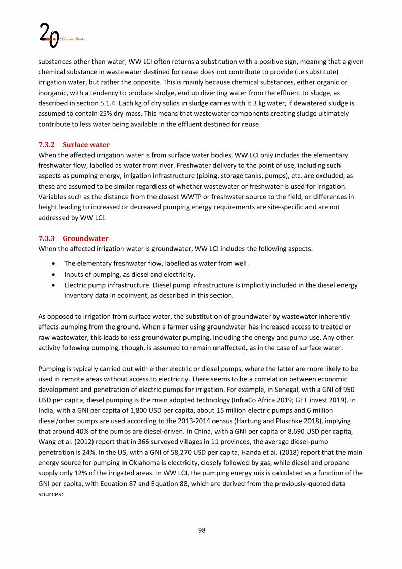
98

substances other than water, WW LCI often returns a substitution with a positive sign, meaning that a given chemical substance in wastewater destined for reuse does not contribute to provide (i.e substitute) irrigation water, but rather the opposite. This is mainly because chemical substances, either organic or inorganic, with a tendency to produce sludge, end up diverting water from the effluent to sludge, as described in section 5.1.4. Each kg of dry solids in sludge carries with it 3 kg water, if dewatered sludge is assumed to contain 25% dry mass. This means that wastewater components creating sludge ultimately contribute to less water being available in the effluent destined for reuse. 7.3.2 Surface water When the affected irrigation water is from surface water bodies, WW LCI only includes the elementary freshwater flow, labelled as water from river. Freshwater delivery to the point of use, including such aspects as pumping energy, irrigation infrastructure (piping, storage tanks, pumps), etc. are excluded, as these are assumed to be similar regardless of whether wastewater or freshwater is used for irrigation. Variables such as the distance from the closest WWTP or freshwater source to the field, or differences in height leading to increased or decreased pumping energy requirements are site-specific and are not addressed by WW LCI. 7.3.3 Groundwater When the affected irrigation water is groundwater, WW LCI includes the following aspects:

The elementary freshwater flow, labelled as water from well. Inputs of pumping, as diesel and electricity. Electric pump infrastructure. Diesel pump infrastructure is implicitly included in the diesel energy

inventory data in ecoinvent, as described in this section. As opposed to irrigation from surface water, the substitution of groundwater by wastewater inherently affects pumping from the ground. When a farmer using groundwater has increased access to treated or raw wastewater, this leads to less groundwater pumping, including the energy and pump use. Any other activity following pumping, though, is assumed to remain unaffected, as in the case of surface water. Pumping is typically carried out with either electric or diesel pumps, where the latter are more likely to be used in remote areas without access to electricity. There seems to be a correlation between economic development and penetration of electric pumps for irrigation. For example, in Senegal, with a GNI of 950 USD per capita, diesel pumping is the main adopted technology (InfraCo Africa 2019; GET.invest 2019). In India, with a GNI per capita of 1,800 USD per capita, about 15 million electric pumps and 6 million diesel/other pumps are used according to the 2013-2014 census (Hartung and Pluschke 2018), implying that around 40% of the pumps are diesel-driven. In China, with a GNI per capita of 8,690 USD per capita, Wang et al. (2012) report that in 366 surveyed villages in 11 provinces, the average diesel-pump penetration is 24%. In the US, with a GNI of 58,270 USD per capita, Handa et al. (2018) report that the main energy source for pumping in Oklahoma is electricity, closely followed by gas, while diesel and propane supply only 12% of the irrigated areas. In WW LCI, the pumping energy mix is calculated as a function of the GNI per capita, with Equation 87 and Equation 88, which are derived from the previously-quoted data sources:

99

Irrdiesel = 17.766 GNI-0.464 Equation 87. Calculation of the groundwater pumping energy mix, diesel component. For GNI values below 490 USD per capita, Irrdiesel becomes higher than 1. In this case a value of 1 is forced in WW LCI. Irrelec = 1 - Irrdiesel

Equation 88. Calculation of the groundwater pumping energy mix, electric component. Where Irrdiesel and Irrelec correspond to the diesel and electric components of the pumping energy mix, respectively and x is the GNI per capita in USD. Figure 17 below plots Irrelec as a function of GNI, showing the simulated values for the previously mentioned countries.

Figure 17. Groundwater pumping from diesel pumps as a function of GNI, calculated with Equation 87. Unitary energy consumption for groundwater lifting (Eground), in MJ per m3, is estimated with Equation 89:

Eground = g · L · m 106 · ƞ

Equation 89. Calculation of energy consumption for groundwater lifting. Where:

g is gravity, 9.8 m/s2.

L is the groundwater table depth. This is estimated as a generic value of 50 m. This compares to an average of 61 m (range 35 to 98 m) according to Wang et al. (2012) in China and 24.4-79.7 m in Oklahoma according to Handa et al. (2018).

m is the mass of water, namely 1,000 kg for 1 m3.

y = 17.766x-0.464

0%

20%

40%

60%

80%

100%

0 10,000 20,000 30,000 40,000 50,000 60,000

Dies

el-p

ump

irrig

atio

n (%

)

GNI per capita (USD)

· Senegal

· India

· China

·

United States

100

Ƞ is the pump efficiency, dimensionless. This is taken as 15% for diesel pumps and 40% for electric pumps (Wang et al. 2012).

The calculated values for Eground correspond to 3.27 MJ per m3 for diesel pumps and 1.23 MJ (0.34 kWh) for electric pumps. Electricity consumption is modelled with the country-specific electricity mixes in ecoinvent. Production of the electric pump is approximated with the ecoinvent data set for a 40 W pump, quantified as 0.00146 units per m3 pumped. This value is obtained as 0.0035 kg pump per m3, as reported in several ecoinvent irrigation data sets, and a 40-W pump weight of 2.43 kg, also obtained from the pump data set in ecoinvent. Diesel pumping is modelled with the ecoivent data set for diesel burned in building machines, which already includes an estimate of machine infrastructure. 7.3.4 Seawater desalination Irrigation water from seawater desalination is modelled with the ecoinvent data set for tap water production by seawater reverse osmosis with ultrafiltration pretreatment, baseline module, single-stage.

7.4 Substituted crops When supply of freshwater for irrigation is considered as a constrained resource and unconventional water supply (desalination) is not an option, an additional supply of irrigation water through treated or untreated wastewater affects crop yields, by increasing them. As a consequence, the additional crop production as a result of increased irrigation substitutes the same amount of crop in the market. In WW LCI, the quantification of the substituted crops is done as follows:

A global water intensification factor is defined, expressed in kg global crop/L irrigation (see section 7.4.1).

A country-specific marginal crop production mix is defined (see section 7.4.2).

The global water intensification factor is applied to the country-specific marginal crop production mix, to calculate the increased crop production (see section 7.4.3).

With this approach, we obtain an estimate of the amounts of particular crops expected to be mainly affected in a given country, when an additional volume of treated or untreated wastewater is made available for irrigation. 7.4.1 Global water intensification factor According to AQUASTAT (2014), in 2011 40% of the World’s crop production took place on irrigated land, corresponding to 20% of the World’s cultivated area. Therefore, the remaining 60% of global crop production was rainfed, produced in 80% of the World’s cultivated area. From this information, it can be calculated that irrigated agriculture is globally 40%/20%*80%/60% = 2.76 times more productive than rainfed agriculture. This global average figure seems to be in agreement with figures for particular crops (corn, alfalfa, cotton, sorghum, soybeans, wheat) in the US, as given by Smidt et al. (2016), reporting that irrigation increases yield by a factor of two to four times relative to dryland farming.

101

In 2011, FAOSTAT reported a global crop production of 8.32E+09 tonnes, of which, as mentioned above, 40% originated in irrigated areas, totalling 3.46E+08 hectares, where the average irrigated volume is 7,700 m3/hectare (AQUASTAT 2014). This results in a global average yield of 9.61 tonnes/irrigated hectare. Given that irrigated agriculture is 2.76 times more productive, we can calculate the global yield of rainfed agriculture as 9.71/2.76 = 3.60 tonnes/hectare. Based on the above figures, we can calculate a global water intensification (WIglo) factor with Equation 90:

WIglo = 9.71 - 3.60

= 0.00078 tonne/m3 7,700

Equation 90. Calculation of a global water intensification factor based on AQUASTAT and FAOSTAT data. Thus, considering all crops produced in all countries, we estimate that in average, 1 additional m3 of water made available for irrigation leads to 0.78 kg of additional harvest. This value is assumed to be appropriate also for irrigation from either treated or untreated wastewater. It could be argued that the latter involves the additional benefit of its higher fertilizer value, leading to even higher WIglo values. In WW LCI, though, fertilization as such is assumed not to be constrained. Therefore, the fertilizer value of wastewater used in irrigation is considered not to result in increased crop yields, but in the substitution of mineral fertilizers, as described in sections 7.1 and 7.2. 7.4.2 Marginal crop mix For each country with a constrained freshwater supply and GNI below 12,535 USD per capita (see section 7.1), WW LCI provides an estimate of a so-called marginal crop mix, attempting to identify which crops are most likely to be affected by an increased availability of irrigation water, and in which proportions they are expected to be affected. It is assumed in the calculations that all crops cultivated in a given country are potentially eligible to receive irrigation. The marginal crop mix is defined using data from FAOSTAT, with the following approach:

An analysis of crop production is done for the period 2013 to 2017 in the particular country, including all individual crops. Only those crops showing a net growth in this period are considered as part of the marginal mix. Net growth is defined as production having a positive slope in the mentioned period.

Crops with a positive growth trend are classified into the following groups: cereals, fruits, horticulture, oilseeds, pulses, roots and tubers, nuts and fibre crops.

Each crop group is assigned a percentage of the crop mix, in proportion to how the individual crops belonging to this group contribute to the total net growth in agricultural production in the country in 2013-2017. When this percentage is lower than 10%, the crop group as a whole is neglected.

Each crop group with a percentage of 10% or more is associated with a model crop, to be considered in WW LCI. The model crops are chosen from the available data sets in ecoinvent, as shown in Table 26. To simplify the model, only one crop is chosen per crop group, even if ecoinvent might have data sets available for more crops falling into the same group. As an example, if the crop group ‘Cereals’ includes wheat and maize but the former has higher net growth trend than the

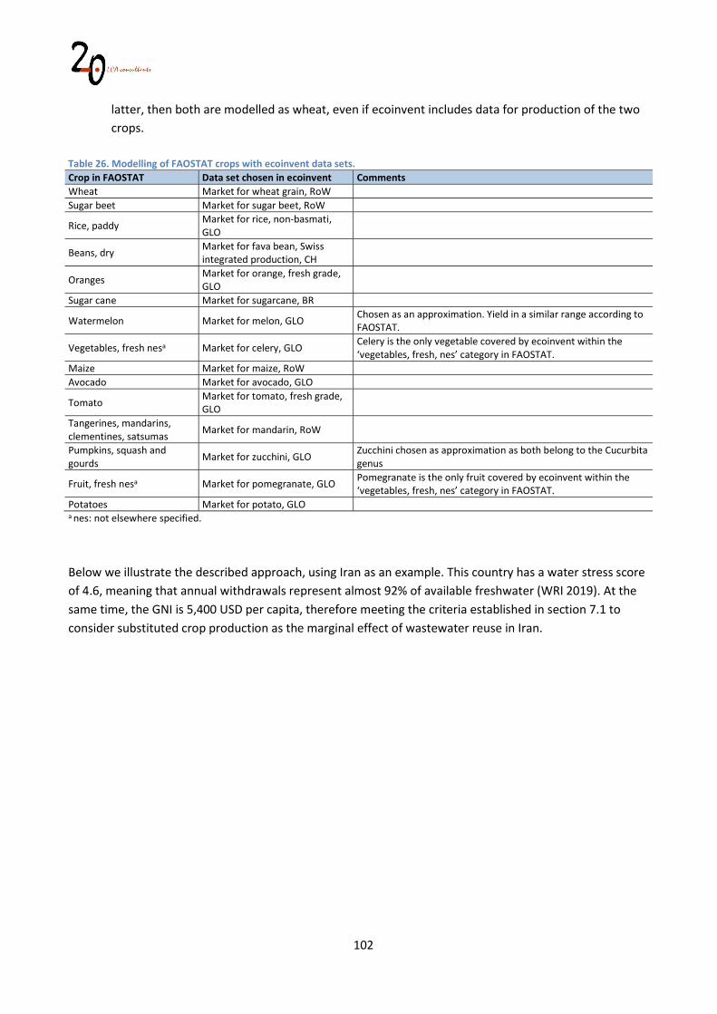
102

latter, then both are modelled as wheat, even if ecoinvent includes data for production of the two crops.

Table 26. Modelling of FAOSTAT crops with ecoinvent data sets. Crop in FAOSTAT Data set chosen in ecoinvent Comments Wheat Market for wheat grain, RoW Sugar beet Market for sugar beet, RoW

Rice, paddy Market for rice, non-basmati, GLO

Beans, dry Market for fava bean, Swiss integrated production, CH

Oranges Market for orange, fresh grade, GLO

Sugar cane Market for sugarcane, BR

Watermelon Market for melon, GLO Chosen as an approximation. Yield in a similar range according to FAOSTAT.

Vegetables, fresh nesa Market for celery, GLO Celery is the only vegetable covered by ecoinvent within the ‘vegetables, fresh, nes’ category in FAOSTAT.

Maize Market for maize, RoW Avocado Market for avocado, GLO

Tomato Market for tomato, fresh grade, GLO

Tangerines, mandarins, clementines, satsumas

Market for mandarin, RoW

Pumpkins, squash and gourds

Market for zucchini, GLO Zucchini chosen as approximation as both belong to the Cucurbita genus

Fruit, fresh nesa Market for pomegranate, GLO Pomegranate is the only fruit covered by ecoinvent within the ‘vegetables, fresh, nes’ category in FAOSTAT.

Potatoes Market for potato, GLO a nes: not elsewhere specified.

Below we illustrate the described approach, using Iran as an example. This country has a water stress score of 4.6, meaning that annual withdrawals represent almost 92% of available freshwater (WRI 2019). At the same time, the GNI is 5,400 USD per capita, therefore meeting the criteria established in section 7.1 to consider substituted crop production as the marginal effect of wastewater reuse in Iran.

103

Table 27. Calculation of a marginal crop mix for Iran.

Crop group Crop 2013

(kt/yr) 2014

(kt/yr) 2015

(kt/yr) 2016

(kt/yr) 2017

(kt/yr)

Trend 2013-2017

(kt/yr)a

Contribution to trend (%)

Crop modelb

Marginal mix (%)c

Cereals

Barley 2,812 2,955 3,202 3,724 3,100 134 4%

Wheat 59% Rice, paddy 2,450 2,347 2,348 2,921 2,639 95 3%

Wheat 9,304 10,579 11,522 14,592 14,000 1,340 43%

Total cereals 14,566 15,881 17,072 21,237 19,739 1,569 50%

Fruit

Dates 1,014 1,033 1,033 1,104 1,185 41 1%

Excluded (<10%)

0% Plums and sloes 193 265 265 263 299 21 1%

Watermelons 3,686 4,011 3,714 4,093 4,060 83 3%

Total fruit 4,893 5,309 5,012 5,460 5,544 145 5%

Horticulture

Eggplants 603 528 653 671 654 24 1%

Excluded (<10%)

0% Lettuce, chicory 224 412 510 528 513 69 2%

Tomatoes 5,757 6,363 6,013 5,829 6,177 31 1%

Total horticulture 6,584 7,303 7,176 7,028 7,344 124 4%

Nuts

Pistachios 225 441 441 406 575 67 2% Excluded (<10%)

0% Walnuts, with shell

223 403 403 368 349 22 1%

Total nuts 448 844 844 774 924 89 3%

Roots and tubers

Onions, dry 2,050 2,066 2,426 2,401 2,379 99 3%

Sugar beet 41%

Potatoes 4,598 4,989 5,141 4,995 5,102 102 3%

Sugar beet 3,467 4,731 5,594 5,966 5,840 598 19%

Sugar cane 6,537 6,589 7,407 7,480 7,562 294 9% Total roots and tubers

16,652 18,375 20,568 20,842 20,883 1,093 35%

Other Several crops 25,114 22,234 20,059 20,309 19,263 117 3% Excluded (<10%)

0%

Total Total 68,257 69,946 70,731 75,650 73,697 3,137 100% - 100% a Average annual growth in the period. Crops with a negative annual growth are excluded. b Crop groups contributing less than 10% to the total crop production growth (3,137 kt/yr in Iran during 2013-2017) are excluded. c Calculated for each crop group as its total divided by the sum of the total for all crop groups not excluded. Example for cereals: 50%/(50%+35%) = 59%.

In Iran, the crops showing the biggest growth in 2013-2017 belong to the groups cereals and roots and tubers. Cereals are dominated by wheat, with smaller contributions from barley and rice, while roots and tubers are dominated by sugar beet, followed by sugar cane, onions and potatoes. Crops included in the groups fruits, horticulture, nuts, and in other constitute less than 10% of annual production growth each, and for this reason they are neglected in the marginal mix, which only includes cereals, modelled as wheat, and roots and tubers, modelled as sugar beet. 7.4.3 Calculation of increased crop production The water intensification factor calculated in section 7.4.1 is a global average one, and cannot directly be applied to specific crops. If 1 additional m3 water is available to irrigate wheat or sugar beet, this cannot be expected in both cases to return an increased production of 0.78 kg wheat or sugar beet, given that these two crops have substantially different yields. An additional m3 available for irrigation would most likely result in more kg of sugar beet than wheat. In this section we address this particular aspect.

104

For a given crop group in a given country, the water intensification factor (WIx) in WW LCI is calculated with Equation 91:

WIx = Wglo Yieldx

Yieldglo

Equation 91. Calculation of a crop-specific water intensification factor. Where Yieldglo is the global average yield (including the contribution of all crops) calculated based on FAOSTAT data for 2011, the reference year for Wglo, which corresponds to 5.55 tonne/ha. Yieldx is the global average yield for crop ‘x’, also for 2011. Following with the example of Iran, we illustrate in Table 28 the calculation of Yieldx, WIx and the increased crop production as a result of 1 additional m3 of water available for irrigation in this country. The resulting estimate is that this will result in an increase of 4.1 kg roots and tubers and 0.34 kg cereals, the former modelled in WW LCI as sugar beet and the latter as wheat. Table 28. Calculation of increased crop production from wastewater irrigation in Iran.

Crop groupa Crop modela Yieldxb

(kg/ha) Wx

(kg crop/m3)c Marginal mix

(%)a Increased production

(kg/m3)e Cereals Wheat 3,164 0.57 59% 0.34 Roots and tubers Sugar beet 54,941 9.9 41% 4.1 a Based on Table 27. b Global average, FAOSTAT data for 2011. c Calculated with Equation 91. e Calculated as Wx · % in marginal mix.

105

8 Water balance

As part of the overall mass balance in the foreground system, WW LCI calculates a water balance. On the one hand, water can be part of the assessed discharges, since wastewater is mostly constituted by water, but water is also generated and consumed in different chemical reactions involving other substances, such as organic matter. For this reason, the model discriminates these two cases in the calculations, namely water initially present in the discharge, and water associated to all other substances.

8.1 Balance for water in wastewater discharges Water entering the system as a component in wastewater ends up as an emission to either air, water, or soil. The amount of water emitted to water is calculated with Equation 92: Waterwater = 1 - Waterair - Watersoil-def - Watersoil-reuse Equation 92. Calculation of the fraction of water emitted to water from wastewater discharges. Where Waterwater is the amount of water initially present in the assessed discharge (in kg/kg discharge) that is emitted to the water environment (surface water, seawater, groundwater). Waterair is the amount of water evaporated in WWTPs and by default this is zero in a Tier 1 assessment. In a Tier 2 assessment, evaporation of water in WWTPs is user-defined, and allowed as input data only for WWTPs with secondary treatment (both activated sludge and stabilization ponds) and for WWTPs with tertiary treatment. Watersoil-

def is the amount of water emitted to soil through open defecation, while Watersoil-reuse is the amount of water emitted to soil through effluents reused in agriculture. These two components for emissions to soil, therefore, are dependent on scenario data, i.e. the percentage of the assessed discharge that originates in open defecation and on the percentage of treated and untreated wastewater effluents being reused in agriculture. The volume of irrigation water substituted thanks to reuse of treated or untreated effluents in agriculture (Waterirr), in L/kg discharge, is calculated with Equation 93: Waterirr = - Watersoil-reuse

Equation 93. Calculation of the irrigation water substituted by water in wastewater discharges. As it can be seen in Equation 93, this volume equals the volume of water emitted to soil through treated or untreated effluents reused in agriculture, with a negative sign. The substituted water can be either surface water, groundwater, or water supplied from desalination, the latter not shown in the inventory as an elementary water flow, but rather as an input of desalinated water (see section 7.3 on substituted irrigation for details).

8.2 Balance for water associated to other substances in wastewater discharges Substances other than water, such as organic and inorganic compounds present in wastewater discharges are also subject to a water balance. This is because they also interact with water. To name a few examples, water is generated as the product of biological and combustion processes, but it is also consumed in

106

anaerobic digestion processes. Therefore, the inventories for organic and inorganic substances include emissions of water to air, water and soil, which are calculated as described below. Emissions of water to the water environment (surface water, seawater, groundwater), are calculated with Equation 94:

Waterwater = (WaterWWTP-aer - WaterWWTP-anaer - WaterWWTP-sludge) · (1 - Freuse-treat) - Watersewer-an · Ftreat

Fsewer· (1 - Freuse-treat) +

Funtreat

Fsewer· (1 - Freuse-untreat)

Equation 94. Calculation of water emitted to water by organic and inorganic substances present in wastewater discharges. Where:

Waterwater is the amount of water, in kg water/kg substance, emitted to water by an organic or inorganic substance in the assessed discharge.

WaterWWTP-aer is the amount of water, in kg water/kg substance, produced by aerobic degradation of the assessed substance in WWTPs with secondary or tertiary treatment (see sections3.3.4 and 3.4.2 and 3.5.4 ). This term also includes water production in septic tanks and stabilization ponds, needed to balance the speciation of ammonia in biogas to N2 and N2O, as described in section 3.8.4.

WaterWWTP-anaer is the amount of water, in kg water/kg substance, consumed by anaerobic degradation of sludge generated by the assessed substance in WWTPs that have an anaerobic digester (see section 5.1.1). This sludge can be constituted by either the assessed substance itself, once partitioned to sludge, or by sludge biomass generated by the biological degradation of the assessed substance in the WWTP.

WaterWWTP-sludge is the amount of water, in kg water/kg substance, in sludge generated by the assessed substance in WWTPs. It refers to the water embedded in the dewatered sludge as it leaves the WWTPs for disposal (see section 5.1.4).

Watersewer-an is the amount of water, in kg water/kg substance, consumed by anaerobic degradation of the assessed substance while flowing through closed sewers (see section 3.1.3).

Freuse-treat is the fraction of treated wastewaters subject to reuse in agriculture. Values are country-specific.

Freuse-untreat is the fraction of untreated wastewaters subject to reuse in agriculture. Values are country-specific.

Ftreat is the fraction of wastewater collected in closed sewers that undergoes treatment in WWTPs. Values are country-specific.

Funtreat is the fraction of wastewater collected in closed sewers that does not undergo treatment in WWTPs. Values are country-specific.

Fsewer is the fraction of wastewater collected in closed sewers. Values are country-specific.

107

Emissions of water to air are calculated with Equation 95: Waterair = WaterWWTP-combustion + Watersludge-incineration - Watersludge-composting

Equation 95. Calculation of water emitted to air by organic and inorganic substances present in wastewater discharges.

Where:

Waterair is the amount of water, in kg water/kg substance, emitted to air by an organic or inorganic substance in the assessed discharge.

WaterWWTP-combustion is the amount of water, in kg water/kg substance, emitted to air by combustion of biogas generated by the assessed substance in WWTPs that have an anaerobic digester (see section 5.1.2).

Watersludge-incineration is the amount of water, in kg water/kg substance, emitted to air by disposal in incineration plants of sludge generated by the assessed substance (see section 5.2.5).

Watersludge-composting is the amount of water, in kg water/kg substance, emitted to air by composting of sludge generated by the assessed substance (see section 5.2.6).

Emissions of water to soil are calculated with Equation 96:

Watersoil = (WaterWWTP-aer - WaterWWTP-anaer - WaterWWTP-sludge) · Freuse-treat - Watersewer-an · Ftreat

Fsewer· Freuse-treat +

Funtreat

Fsewer· Freuse-untreat + Watersludge-land

Equation 96. Calculation of water emitted to soil by organic and inorganic substances present in wastewater discharges. Where:

Watersoil is the amount of water, in kg water/kg substance, emitted to soil by an organic or inorganic substance in the assessed discharge.

Watersludge-land is the amount of water, in kg water/kg substance, emitted to soil as a component of sludge or compost generated by the assessed substance (see section 5.2.7).

The volume of irrigation water substituted thanks to reuse of treated or untreated effluents in agriculture (Waterirr), in L/kg discharge, is calculated with Equation 97:

Waterirr = - (WaterWWTP-aer - WaterWWTP-anaer - WaterWWTP-sludge) · Freuse-treat + Watersewer-an · Ftreat

Fsewer· Freuse-treat +

Funtreat

Fsewer· Freuse-untreat

Equation 97. Calculation of the irrigation water substituted by organic and inorganic substances present in wastewater discharges.

108

As it can be seen, Equation 97 is similar to Equation 96 (water emitted to soil), as it contains the same terms except Watersludge-land, and with the additional difference that signs are reversed, in order to reflect the substitution. Thus, the amount of irrigation water being substituted equals the amount of water emitted to soil through treated or untreated effluents, and we exclude in this calculation the water embedded in sludge applied to agricultural land. The substituted water can be either surface water, groundwater, or water supplied from desalination, the latter not shown in the inventory as an elementary water flow, but rather as an input of desalinated water (see section 7.3 on substituted irrigation for details).

109

9 Uncertainty

In WW LCI each flow is attributed a mean value and an uncertainty factor, attempting to quantify its variation assuming a lognormal distribution, as done in the ecoinvent database (Weidema et al. 2013). The uncertainty factor corresponds to the square of the geometric standard deviation (σg

2), reflecting the 95% confidence interval. As an example, for a value of σg

2 = 1.5, the lower bound of the confidence interval is calculated as the mean divided by 1.5, while the upper bound is calculated as the mean times 1.5. These bounds are expected to contain 95% of the measured values. It must be highlighted, though, that WW LCI does not include a systematic implementation of uncertainty by propagating the error in each variable used in the model. Instead, the same approach as implemented in the ecoinvent database is used, where σg

2 is calculated with Equation 98:

σg2 = e [ ln (U1)]2 + [ ln (U2)]2 + [ ln (U3)]2 + [ ln (U4)]2 + [ ln (U5)]2 + [ ln (Ub)]2

Equation 98. Calculation of the geometric standard deviation (σg2). Where:

Ub corresponds to the basic uncertainty factor (see section 9.1).

U1, U2, U3, U4 and U5 correspond to the uncertainty factors for reliability, completeness, temporal correlation, geographic correlation and technological correlation, respectively. These factors are estimated using data quality indicators (see section 9.2).

9.1 Basic uncertainty factors

According to Weidema et al. (2013) the basic uncertainty factors express variability and stochastic error of the values describing the exchanges, due to e.g. measurement uncertainties, activity-specific variations, temporal variations, etc. Table 29 displays the factors used, based on Frischknecht et al. (2007).

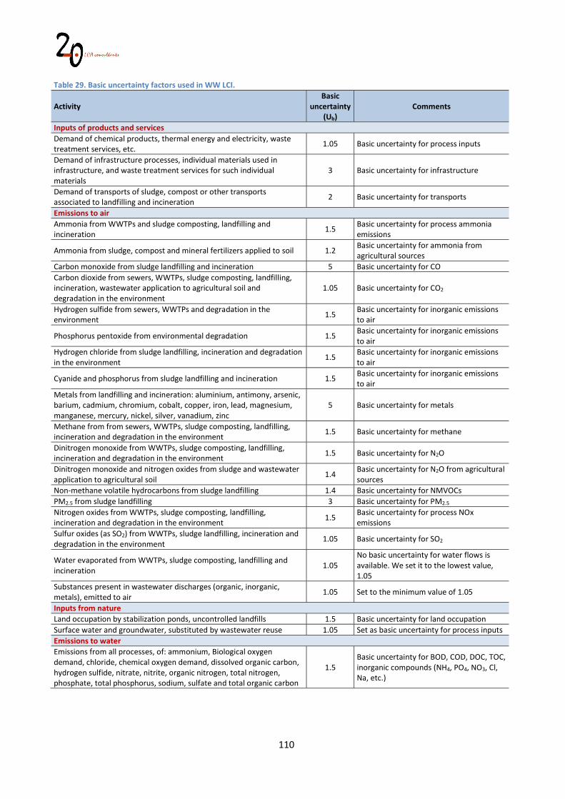
110

Table 29. Basic uncertainty factors used in WW LCI.

Activity Basic

uncertainty (Ub)

Comments

Inputs of products and services Demand of chemical products, thermal energy and electricity, waste treatment services, etc.

1.05 Basic uncertainty for process inputs

Demand of infrastructure processes, individual materials used in infrastructure, and waste treatment services for such individual materials

3 Basic uncertainty for infrastructure

Demand of transports of sludge, compost or other transports associated to landfilling and incineration

2 Basic uncertainty for transports

Emissions to air Ammonia from WWTPs and sludge composting, landfilling and incineration

1.5 Basic uncertainty for process ammonia emissions

Ammonia from sludge, compost and mineral fertilizers applied to soil 1.2 Basic uncertainty for ammonia from agricultural sources

Carbon monoxide from sludge landfilling and incineration 5 Basic uncertainty for CO Carbon dioxide from sewers, WWTPs, sludge composting, landfilling, incineration, wastewater application to agricultural soil and degradation in the environment

1.05 Basic uncertainty for CO2

Hydrogen sulfide from sewers, WWTPs and degradation in the environment 1.5

Basic uncertainty for inorganic emissions to air

Phosphorus pentoxide from environmental degradation 1.5 Basic uncertainty for inorganic emissions to air

Hydrogen chloride from sludge landfilling, incineration and degradation in the environment

1.5 Basic uncertainty for inorganic emissions to air

Cyanide and phosphorus from sludge landfilling and incineration 1.5 Basic uncertainty for inorganic emissions to air

Metals from landfilling and incineration: aluminium, antimony, arsenic, barium, cadmium, chromium, cobalt, copper, iron, lead, magnesium, manganese, mercury, nickel, silver, vanadium, zinc

5 Basic uncertainty for metals

Methane from from sewers, WWTPs, sludge composting, landfilling, incineration and degradation in the environment

1.5 Basic uncertainty for methane

Dinitrogen monoxide from WWTPs, sludge composting, landfilling, incineration and degradation in the environment 1.5 Basic uncertainty for N2O

Dinitrogen monoxide and nitrogen oxides from sludge and wastewater application to agricultural soil

1.4 Basic uncertainty for N2O from agricultural sources

Non-methane volatile hydrocarbons from sludge landfilling 1.4 Basic uncertainty for NMVOCs PM2.5 from sludge landfilling 3 Basic uncertainty for PM2.5 Nitrogen oxides from WWTPs, sludge composting, landfilling, incineration and degradation in the environment 1.5

Basic uncertainty for process NOx emissions

Sulfur oxides (as SO2) from WWTPs, sludge landfilling, incineration and degradation in the environment

1.05 Basic uncertainty for SO2

Water evaporated from WWTPs, sludge composting, landfilling and incineration

1.05 No basic uncertainty for water flows is available. We set it to the lowest value, 1.05

Substances present in wastewater discharges (organic, inorganic, metals), emitted to air

1.05 Set to the minimum value of 1.05

Inputs from nature Land occupation by stabilization ponds, uncontrolled landfills 1.5 Basic uncertainty for land occupation Surface water and groundwater, substituted by wastewater reuse 1.05 Set as basic uncertainty for process inputs Emissions to water Emissions from all processes, of: ammonium, Biological oxygen demand, chloride, chemical oxygen demand, dissolved organic carbon, hydrogen sulfide, nitrate, nitrite, organic nitrogen, total nitrogen, phosphate, total phosphorus, sodium, sulfate and total organic carbon

1.5 Basic uncertainty for BOD, COD, DOC, TOC, inorganic compounds (NH4, PO4, NO3, Cl, Na, etc.)

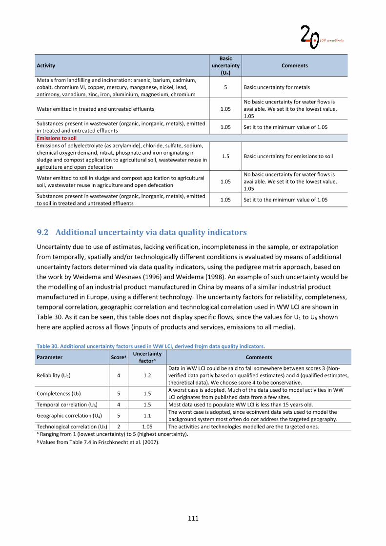
111

Activity Basic

uncertainty (Ub)

Comments

Metals from landfilling and incineration: arsenic, barium, cadmium, cobalt, chromium VI, copper, mercury, manganese, nickel, lead, antimony, vanadium, zinc, iron, aluminium, magnesium, chromium

5 Basic uncertainty for metals

Water emitted in treated and untreated effluents 1.05 No basic uncertainty for water flows is available. We set it to the lowest value, 1.05

Substances present in wastewater (organic, inorganic, metals), emitted in treated and untreated effluents 1.05 Set it to the minimum value of 1.05

Emissions to soil Emissions of polyelectrolyte (as acrylamide), chloride, sulfate, sodium, chemical oxygen demand, nitrat, phosphate and iron originating in sludge and compost application to agricultural soil, wastewater reuse in agriculture and open defecation

1.5 Basic uncertainty for emissions to soil

Water emitted to soil in sludge and compost application to agricultural soil, wastewater reuse in agriculture and open defecation

1.05 No basic uncertainty for water flows is available. We set it to the lowest value, 1.05

Substances present in wastewater (organic, inorganic, metals), emitted to soil in treated and untreated effluents

1.05 Set it to the minimum value of 1.05

9.2 Additional uncertainty via data quality indicators

Uncertainty due to use of estimates, lacking verification, incompleteness in the sample, or extrapolation from temporally, spatially and/or technologically different conditions is evaluated by means of additional uncertainty factors determined via data quality indicators, using the pedigree matrix approach, based on the work by Weidema and Wesnaes (1996) and Weidema (1998). An example of such uncertainty would be the modelling of an industrial product manufactured in China by means of a similar industrial product manufactured in Europe, using a different technology. The uncertainty factors for reliability, completeness, temporal correlation, geographic correlation and technological correlation used in WW LCI are shown in Table 30. As it can be seen, this table does not display specific flows, since the values for U1 to U5 shown here are applied across all flows (inputs of products and services, emissions to all media). Table 30. Additional uncertainty factors used in WW LCI, derived frojm data quality indicators.

Parameter Scorea Uncertainty

factorb Comments

Reliability (U1) 4 1.2 Data in WW LCI could be said to fall somewhere between scores 3 (Non-verified data partly based on qualified estimates) and 4 (qualified estimates, theoretical data). We choose score 4 to be conservative.

Completeness (U2) 5 1.5 A worst case is adopted. Much of the data used to model activities in WW LCI originates from published data from a few sites.

Temporal correlation (U3) 4 1.5 Most data used to populate WW LCI is less than 15 years old.

Geographic correlation (U4) 5 1.1 The worst case is adopted, since ecoinvent data sets used to model the background system most often do not address the targeted geography.

Technological correlation (U5) 2 1.05 The activities and technologies modelled are the targeted ones. a Ranging from 1 (lowest uncertainty) to 5 (highest uncertainty). b Values from Table 7.4 in Frischknecht et al. (2007).

112

9.3 Limitations

The implementation of the described approach to uncertainty in WW LCI currently has the limitations that the calculated σg

2 values are flow-specific, but they are not substance- or country-specific. As an example, methane emissions receive a σg

2 = 1.879, calculated with Equation 98. This value is used for methane flows originating from all types of processes, such as degradation in the environment, stabilization ponds, or combustion of biogas in WWTPs and landfills. Also, this same value is applied to methane produced by different substances present in wastewater. For example, methane generated by two substances such as ethanol and ibuprofen will be assigned the same σg

2 value, 1.879. Finally, there is also no difference in uncertainty with regard to the geographic context. As an example, methane emissions from landfilling of sludge in countries A, B and C will also be assigned the same σg

2 value.

113

10 Linking of inventory data in SimaPro

10.1 Linking to ecoinvent data sets

The entire background system in WW LCI is linked to the corresponding ecoinvent regional market data sets. As an example, hydrochloric acid is supplied in European (RER) and Rest-of-the-World (RoW) markets, which are both used by WW LCI depending on the country under assessment, i.e. wastewater discharges in Spain link to the RER market, while discharges in Argentina link to the RoW market. However, for many data sets only a global market is included, and this is used for all countries. Some particular cases must be mentioned:

Tap water from desalination: a market data set for desalinated water is not currently available in ecoinvent, therefore, a global production data set is used.

Crops: for some of the crops modelled (see section 7.4.2), a global market data set is not available. In these cases, the RoW market data set is used, with the exception of sugarcane and fava beans, where the Brazilian and Swiss market data sets, respectively, are used.

10.2 Regionalization of water flows

Elementary flows of water in WW LCI are regionalized in the same way as done in the ecoinvent database as implemented in the SimaPro software. Water abstraction and discharges are labelled according to the scenario data settings in WW LCI, i.e. at the country level. However, WW LCI also includes flows of water discharged to soil, as a result of wastewater and sludge application in agriculture and discharges through open defecation. Water emissions to soil are currently not implemented in the ecoinvent database, however these flows are included in WW LCI to close the water balance. These flows of water emitted to soil are also regionalized. It must be highlighted that in a Tier 2 assessment, water as part of a wastewater mixture entered by the user is not automatically labelled with the regional tag by WW LCI. In such Tier 2 assessments the regionalization must be manually done by the user, when declaring water as an input substance in the mixture. This is further explained in the user manual.

10.3 Emission sub-compartments

All emissions to air, water and soil in WW LCI are ultimately specified with the following sub-compartments used in the SimaPro software:

For air emissions: high population/low population. For water emissions: river/ocean/groundwater/groundwater-long term. For soil emissions: agricultural/forestry.

The sub-compartment for emissions to air occurring in WWTPs is chosen taking the same assumptions as in ecoinvent for this same activity (urban wastewater treatment), that is, that emissions take place in a high-population density location. Emissions to air associated to composting are also modelled as taking place in a high-population density location.

114

The sub-compartment for emissions to water depends on the activity generating the emission. Discharges of wastewater from sewers or WWTPs use the sub-compartment river and/or ocean, while discharges from septic tanks and latrines use the sub-compartment groundwater. Emissions to water from landfilling and incineration take the same sub-compartments as these same activities in ecoinvent (Doka 2007). Concerning emissions to soil, those originating in sludge application in agriculture use the agricultural sub-compartment, while emissions from open defecation use the forestry sub-compartment.

115

11 Linking of inventory data in GaBi

11.1 Linking to ecoinvent data sets

The entire background system in WW LCI is linked to ecoinvent. However, in GaBi the linking of technosphere flows listed in the inventory to particular ecoinvent activities is done manually. In this way, WW LCI only names the flows, while the user is responsible for choosing the right market data set, such as RER, RoW, etc.

11.2 Regionalization of water flows

Water flows in inventories for export to GaBi are regionalized in the same way as done for SimaPro, therefore the description in section 10.2 applies to GaBi as well.

11.3 Emission sub-compartments

All emissions to air, water and soil in WW LCI are ultimately specified with the following sub-compartments used in the GaBi software:

For air emissions: no sub-compartments are available. For water emissions: fresh water/fresh water long-term/sea water. For soil emissions: agricultural/industrial.

There are no sub-compartments specified for emissions to air, given that GaBi does not currently support any sub-compartment. Concerning emissions to water, the sub-compartment for emissions to water depends on the activity generating the emission. Discharges of wastewater from sewers or WWTPs use the sub-compartment fresh water and/or sea water, while emissions from landfills after 100 years are labelled as emissions to fresh water, long-term. However, discharges from septic tanks and latrines use the sub-compartment fresh water, even though in WW LCI these emissions are modelled as releases to groundwater. However, GaBi does not currently specify a groundwater sub-compartment for emissions to water. Concerning emissions to soil, those originating in sludge application in agriculture use the agricultural soil sub-compartment, while emissions from open defecation use the industrial soil sub-compartment.

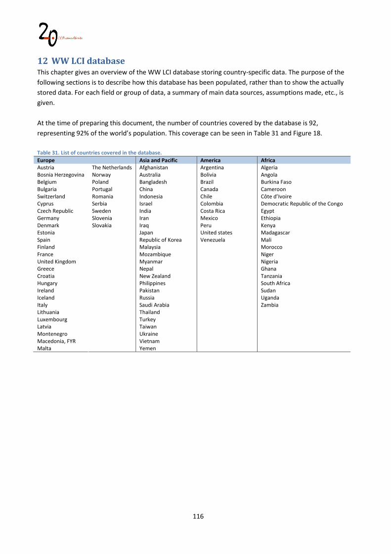
116

12 WW LCI database This chapter gives an overview of the WW LCI database storing country-specific data. The purpose of the following sections is to describe how this database has been populated, rather than to show the actually stored data. For each field or group of data, a summary of main data sources, assumptions made, etc., is given. At the time of preparing this document, the number of countries covered by the database is 92, representing 92% of the world’s population. This coverage can be seen in Table 31 and Figure 18. Table 31. List of countries covered in the database. Europe Asia and Pacific America Africa Austria Bosnia Herzegovina Belgium Bulgaria Switzerland Cyprus Czech Republic Germany Denmark Estonia Spain Finland France United Kingdom Greece Croatia

Hungary Ireland Iceland Italy Lithuania Luxembourg Latvia Montenegro Macedonia, FYR Malta

The Netherlands Norway Poland Portugal Romania Serbia Sweden Slovenia Slovakia

Afghanistan Australia Bangladesh China Indonesia Israel India Iran Iraq Japan Republic of Korea Malaysia Mozambique Myanmar Nepal New Zealand Philippines Pakistan Russia Saudi Arabia Thailand Turkey Taiwan Ukraine Vietnam Yemen

Argentina Bolivia Brazil Canada Chile Colombia Costa Rica Mexico Peru United states Venezuela

Algeria Angola Burkina Faso Cameroon Côte d’Ivoire Democratic Republic of the Congo Egypt Ethiopia Kenya Madagascar Mali Morocco Niger Nigeria Ghana Tanzania South Africa Sudan Uganda Zambia

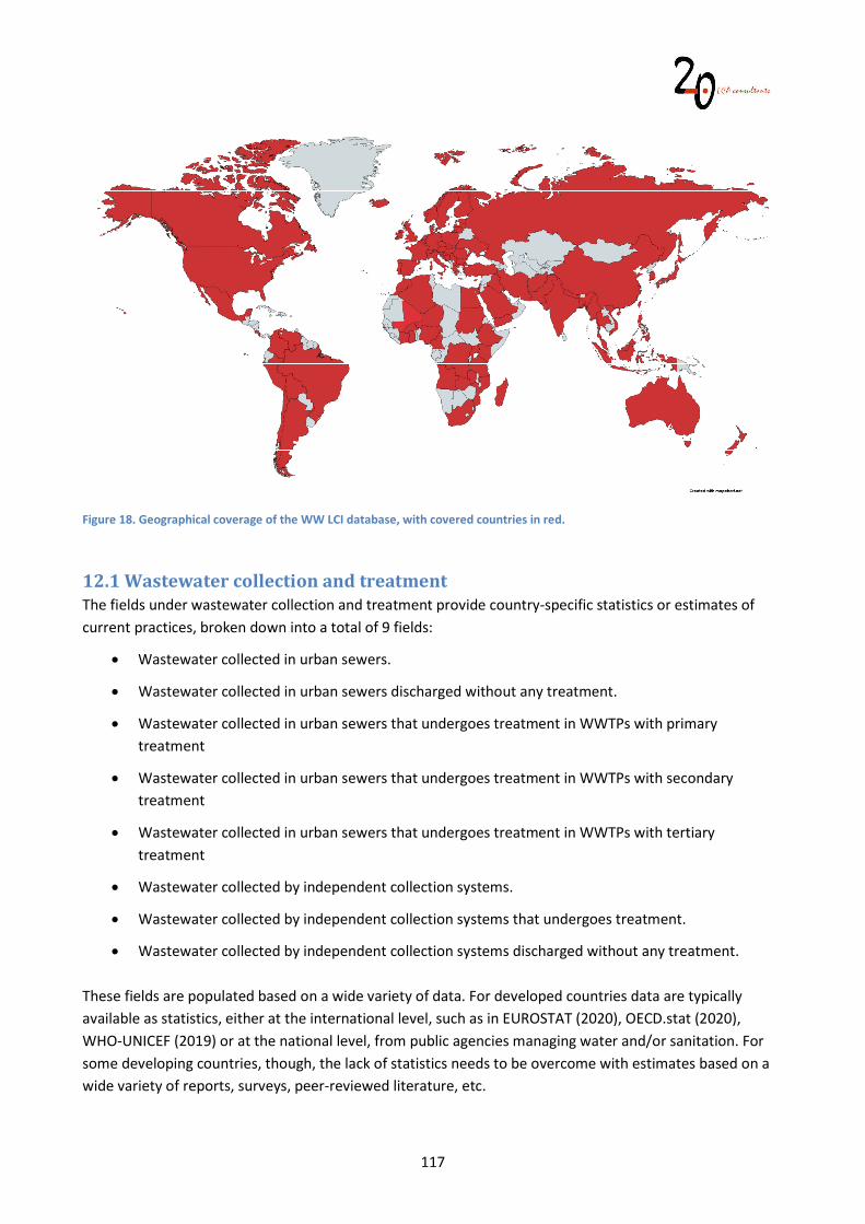
117

Figure 18. Geographical coverage of the WW LCI database, with covered countries in red.

12.1 Wastewater collection and treatment The fields under wastewater collection and treatment provide country-specific statistics or estimates of current practices, broken down into a total of 9 fields:

Wastewater collected in urban sewers.

Wastewater collected in urban sewers discharged without any treatment.

Wastewater collected in urban sewers that undergoes treatment in WWTPs with primary treatment

Wastewater collected in urban sewers that undergoes treatment in WWTPs with secondary treatment

Wastewater collected in urban sewers that undergoes treatment in WWTPs with tertiary treatment

Wastewater collected by independent collection systems.

Wastewater collected by independent collection systems that undergoes treatment.

Wastewater collected by independent collection systems discharged without any treatment. These fields are populated based on a wide variety of data. For developed countries data are typically available as statistics, either at the international level, such as in EUROSTAT (2020), OECD.stat (2020), WHO-UNICEF (2019) or at the national level, from public agencies managing water and/or sanitation. For some developing countries, though, the lack of statistics needs to be overcome with estimates based on a wide variety of reports, surveys, peer-reviewed literature, etc.

118

Figures in these fields sometimes refer to percentages of wastewater volumes, while in other cases they refer to the percentage of population with access to each of the reported options. For all countries a field with data sources is provided, summarizing data sources and assumptions. In the model, urban sewers are assumed to be closed, while direct discharges through independent collection systems are assumed to be open (see section 3.2). Treatment for independent collection systems is assumed as septic tanks in all cases.

12.2 Sludge disposal Sludge disposal statistics reflect the fate of sludge leaving WWTPs as dewatered sludge. Four options are included: composting, reuse in agriculture, landfilling and incineration. It must be highlighted that composting is a treatment rather than a disposal option. The obtained compost is then linked in the model to reuse in agriculture. Also, landfilling is discriminated in the model as either controlled or uncontrolled, as explained in section 12.6. As in wastewater collection and treatment, sludge disposal statistics are populated based on a wide variety of data, including EUROSTAT (2020) for European countries, while for other countries national reports from public agencies are used. For some developing countries, though, the lack of statistics needs to be overcome with estimates based on a wide variety of reports, surveys, peer-reviewed literature, etc. In general, though, the amount on information on disposal of wastewater sludge is substantially lower than that available on wastewater management and for this reason, for many countries, especially developing ones, data could not be found. In such cases, we opted for assuming a disposal mix consisting of 50% landfilling and 50% reuse in agriculture.

12.3 Mean annual and monthly temperatures Mean annual and monthly temperatures in ºC are used in WW LCI to calculate thermal energy demand in WWTPs (see section 6.2) as well as the MCF for open sewers (see section 3.2.3) and the degradation factor in closed sewers (see section 3.1.4). In general, temperature data for all countries have been obtained from Weatherbase (2020).

12.4 Wastewater discharge in inland waters This field expresses the percentage of wastewater discharged in inland environments, as opposed to coastal environments, which add up to the remaining percentage. The former is assumed to receive wastewater in freshwater aquatic environments such as rivers or lakes, while the latter are assumed to receive it in seawater (see section 10.3). Country-specific figures were established based on several sources:

For most European countries we calculated this based on the PE discharged by WWTPs in each country according to the database Waterbase-UWWTD (European Environment Agency 2017), considering discharges to freshwater and to land catchment of freshwater as inland waters, as opposed to discharges in the coast, estuaries, etc.

119

For a few countries we used data from Hauschild and Potting (2005, annex 1).

For most remaining countries we made the assumption that the percentage of discharges to the ocean is equal to the percentage of the country’s population that lives in the coast. This is approximated with data from CIESIN (2012) reporting the percentage of population living within 10 km of the coast.

12.5 Capacity of WWTPs For all countries in the WW LCI database a WWTP capacity mix and sewer capacity mix are provided. In practice, only the WWTP capacity mix is provided, which is then matched with an equivalent sewer capacity. The WWTP capacity mix not only influences the impact of wastewater infrastructure, but also the electricity consumption associated to the WWTPs, as described in section 6.1.1. For each country, the WWTP capacity mix states 1) the percentage of wastewater treated under each one of the five infrastructure classes and 2) the average capacity of the WWTPs within each class. For each country a short explanation is given, as well as the data sources/assumptions made, although the actual calculation of the capacity mix is not shown. These calculations are available to WW LCI users upon request. The number of data sources to fill in this information at the country level is too long for an itemized discussion in this report, however all references are available in the database. In short, we could describe the data sources as follows:

For European countries we used the database Waterbase-UWWTD (European Environment Agency 2017). This database contains an inventory of European WWTPs including numerous descriptors, among which the design and actual treatment capacity, expressed as PE. The country mixes were derived from these data, by converting from PE to m3/d, the latter based on wastewater production per person according to EUROSTAT (2018a), AQUASTAT (2018) or other sources.

For a few countries we were able to use detailed inventories reporting on all the existing WWTPs in the country.

In many cases we used technical reports, peer-reviewed articles, etc., which provided a more or less complete distribution of the existing WWTPs in a few capacity classes. In such cases it was necessary to assume a certain average size for each capacity. For example, if a number of plants were reported to be between 20,000 and 40,000 m3/d, we typically took the average, 30,000 m3/d to represent this capacity class.

Finally, in some cases it was not possible to obtain an actual mix, since the only data found were the total number of WWTPs and their total treatment capacity. In this case only one infrastructure class is used.

12.6 Controlled and uncontrolled landfilling of sludge

We have not found any statistics or studies covering sludge landfilling practices in different countries that could allow us to label these practices according to the options included in WW LCI, i.e. controlled or uncontrolled (see sections 5.2.3 and 5.2.4). We have attempted to estimate these practices, assuming that the level of control in landfilling of sludge in a country is correlated with the level of economic

120

development, which we measure as the gross national income (GNI) per capita, with data from the World Bank (2018). We expect developed countries to rely on controlled sanitary landfills, whereas developing countries are expected to rely mainly on less controlled landfills. We have established the following key GNI levels:

A GNI level of 35,000 USD per capita is defined as the point at which 100% of the landfilling activity takes place in controlled facilities. This leaves out certain countries classified as advanced economies by the IMF, such as Italy (31,020 USD per capita) Spain (27,180 USD per capita) or Greece (18,090USD per capita). There is evidence, though, that landfilling of solid waste in these countries still happens (probably to a low extent) under uncontrolled conditions (see Revuelta 2017; Reuters 2014; Perchard 2016).

A GNI level of 2,500 USD per capita is defined as the point below which 0% of the landfilling activity takes place in controlled facilities. Under this threshold we find countries such as India (1,820 USD per capita) Vietnam (2,170 USD per capita) or Ukraine (2,390 USD per capita).

Based on the two coordinates above (x, y): (35000, 1), (2500, 0) and (0, 0) we defined a logistic curve as shown in Figure 19, where we show how several countries fit into this model. This function allows us to calculate the percentage of controlled landfilling, whereas the difference between this and 100% is the percentage of uncontrolled landfilling.

Figure 19. Curve used to estimate controlled landfilling. As GNI increases, the percentage of sludge to controlled landfills respect to total landfilling. At 35,000 USD only controlled landfilling is available.

12.7 Anaerobic digestion and cogeneration in WWTPs

The database attempts to provide the following variables for each country:

The percentage of wastewater treated in WWTPs with AD. The percentage of wastewater treated in WWTPs with AD and CHP.

0%

10%

20%

30%

40%

50%

60%

70%

80%

90%

100%

0 5000 10000 15000 20000 25000 30000 35000 40000 45000

Cont

roll

ed la

ndfil

l/to

tal l

andf

ill

GNI (USD per capita)

India

·

China

·

Chile

· ·

Germany

121

In this report we do not describe in detail how these percentages were calculated for each country. Instead, we describe the main data sources, assumptions and limitations. The detailed calculations are available to the WW LCI user upon request. For European countries the percentage of AD was estimated based on two main variables: the annual amount of primary energy produced from biogas in WWTPs and the annual amount of sludge produced. Biogas production in 2016, expressed as ktoe, was obtained from the Biogas Barometer (EurObserv’ER 2017), which publishes this information for the EU28, disaggregated by country and for three sectors (landfills, sewage, and other e.g. municipal solid waste, agricultural waste). The percentage of sludge treated with AD (%AD) was calculated with Equation 99:

%AD = Sludge_to_AD

0.375 · Sludge_to_AD + Final_sludge Equation 99. Calculation of the percentage of sludge treated in WWTPs with anaerobic digestion. Where Sludge_to_AD is an estimate of the amount of raw sludge sent to anaerobic digestion (kg dry mass/year) and Final_sludge is the declared amount of sludge sent for disposal (kg dry mass/year). The value of 0.375 is the ratio of kg total solids destroyed per kg solids sent to anaerobic digestion, which originates from assuming 0.75 kg VSS/kg raw sludge and 50% destruction of VSS in the AD process (see section 6.2.1). The parameter Sludge_to_AD is calculated as: Sludge_to_AD = Biogas · 8.625 Equation 100. Calculation of raw sludge produced in WWTPs with anaerobic digestion (kg dry mass/year). Where Biogas is the annual biogas production as primary energy, in MJ/year, and 8.625 is our estimate of biogas energy produced per unit of raw sludge sent to the AD process, in MJ/kg dry mass. This factor originates from taking the above factor of 0.375 kg solids destroyed/kg dry mass and further assuming 1 m3 biogas/kg solids destroyed and a net calorific value of 23 MJ/m3 biogas (see section 6.2.1). Besides the theoretical nature of this calculation procedure, another limitation or source of uncertainty is related to the original data on biogas production and sludge production. Concerning the former, the Biogas Barometer reports biogas production by the sewage sector, but this includes not only municipal but also industrial WWTPs. We tried to compensate this by including industrial sludge production from Eurostat in our calculations, however for most countries industrial sludge is not reported in EUROSTAT (2018b). Secondly, sludge production for the same country sometimes varies substantially from year to year, even in countries where wastewater infrastructure is already developed and no significant changes should be expected. For example, in Austria in 2014 the amount of sludge (in dry mass) decreased by 11% compared to 2011. In our calculations we did not take these fluctuations into account, by always choosing the latest data point available. Last but not least, it must be highlighted that the two sets of data referred to different years, with the biogas data referring to 2016 (latest available), while sludge production ranged from 2009 to 2015 depending on the country.

122

This approach led to coherent results for 27 out 28 countries, where by coherent results we define a value for %AD that does not exceed 100%. The exception was Bulgaria, where we obtained %AD = 101%. In the database we set this to 100%, however we think this is probably overestimated, maybe due to either the inclusion of biogas production from industrial WWTPs, inaccurate data on sludge production or unrealistic assumptions from our side in the energy and mass balance of the AD process. The penetration of CHP systems, in the case of EU countries, was based on figure 6 in Kampman et al. (2016), reporting percentage of biogas used for electricity, heat and biomethane. Here we assumed that only use for electricity production represents CHP systems. One limitation of these data is that it reflects the utilization of biogas by the entire biogas industry in each country, which might deviate from the specific WWTP sector. The calculation procedure presented in the above paragraphs was also applied to Brazil, Korea and Norway, but using data from IEA (2017) for quantifying annual biogas production and utilization of biogas in CHP systems, while several other sources were used to quantify (sometimes crudely estimate) annual sludge production. For other countries we used technical reports, peer-reviewed literature, conference presentations, etc., often requiring additional assumptions from our side. For example, for US we used the study by ERG (2011) prepared for the USEPA, where it is stated that 60% of wastewater is treated in WWTPs with AD, however the penetration of CHP systems is quantified as installed capacity in MW. We estimated the capacity of the WWTPs with these installed MW assuming 26 kW/Mgal wastewater, based on the theoretical model they present to study the potential of CHP systems in the country. This estimated capacity can be then expressed as a percentage of the country’s WWTP capacity as a whole. Another example is Canada, where we only found data for the State of Ontario (Environmental Commissioner of Ontario 2017, p. 138), which we took as an approximation for the entire country. In addition to this, the data for Ontario are reported in percentage of facilities, without weighting for their capacity. In developing countries, data availability for this topic is not good either. In many countries the wastewater treatment sector is in such an early stage of development that the lack of information is just a reflection of the lack of this kind of infrastructure in the first place; in many cases we assumed there is 0% AD, for example Tanzania and Pakistan. In other countries, the lack of AD and CHP infrastructure is supported by actual reports, for example in Saudi Arabia (Saudi Arabian Water Environment Association 2013) while in other countries where AD is applied, it was necessary to investigate which individual facilities have installed AD systems, as was the case for Ukraine and Russia, among others. Overall, our percentages of AD and CHP can be considered as a starting point, in spite of the substantial uncertainty. The percentage of CHP is even more uncertain, as it adds up the uncertainty on the occurrence of CHP systems on top of the uncertainty on the occurrence of AD.

12.8 Methane factors for closed sewers, open sewers and latrines

This part of the database contains country-specific values for the degradation factor in closed sewers (Degclosed) and methane correction factors for open sewers (MCFopen) and latrines (MCFlat). These are calculated as described in sections 3.1.4, 3.2.3 and 3.10.2, respectively. The calculation of MCFlat requires data on average precipitation for each country, which listed as obtained from World Bank (2020b).

123

12.9 Open defecation and latrine use Contains statistics on the percentage of population practicing open defecation (Popdef), taken from World Bank (2019) and the calculated percentage of population using latrines (Poplat), which is calculated with Equation 101: Poplat = Popind-coll - Popseptic - Popdef

Equation 101. Calculation of the percentage of population using latrines. Where Popind-coll is the percentage of population with access to independent wastewater collection systems and Popseptic is the percentage of population with access to independent wastewater collection systems that uses septic tanks. Both values are obtained as described in section 12.1.

12.10 Septage disposal WW LCI discriminates between safely disposed and unsafely disposed septage, with the former modelled as treated in a centralized WWTP (see section 5.1.3), while the latter is modelled as a direct discharge to the aquatic environment (see section 5.2.9). Given the lack of a single source of statistics on this topic, the following procedure has been established in the database in order to determine a country-specific percentage of controlled vs. uncontrolled septage disposal:

For advanced economies as defined by the IMF (2020), it is assumed that 100% of septic sludge is safely disposed.

For a total of 30 countries, an estimate is made based on data reported in Shit Flow Diagrams (SFD) published by the Sustainable Sanitation Alliance (SuSanA 2020), as explained below.

For the remaining countries, the percentage of controlled septage disposal is estimated as a function of GNI per capita, as explained below.

SFD studies report in a visual format how human excreta is managed in a given city or town, including such aspects as types of collection, treatment and ultimate disposal. Among other data, they report the percentage of faecal sludge that is emptied (including septic tanks but also latrines), and the percentage of faecal sludge that receives appropriate treatment. The ratio treated/emptied is adopted in WW LCI as the percentage of controlled septage disposal. In order to scale up the data from cities to countries, this ratio is calculated for all cities with a published SFD in a given country, and a population-weighted average ratio is calculated. As an example, Table 32 shows the calculation of this weighted average for Ethiopia, based on data reported for six cities. Whenever only data for one city are available, this is used as representative value for the country as a whole.

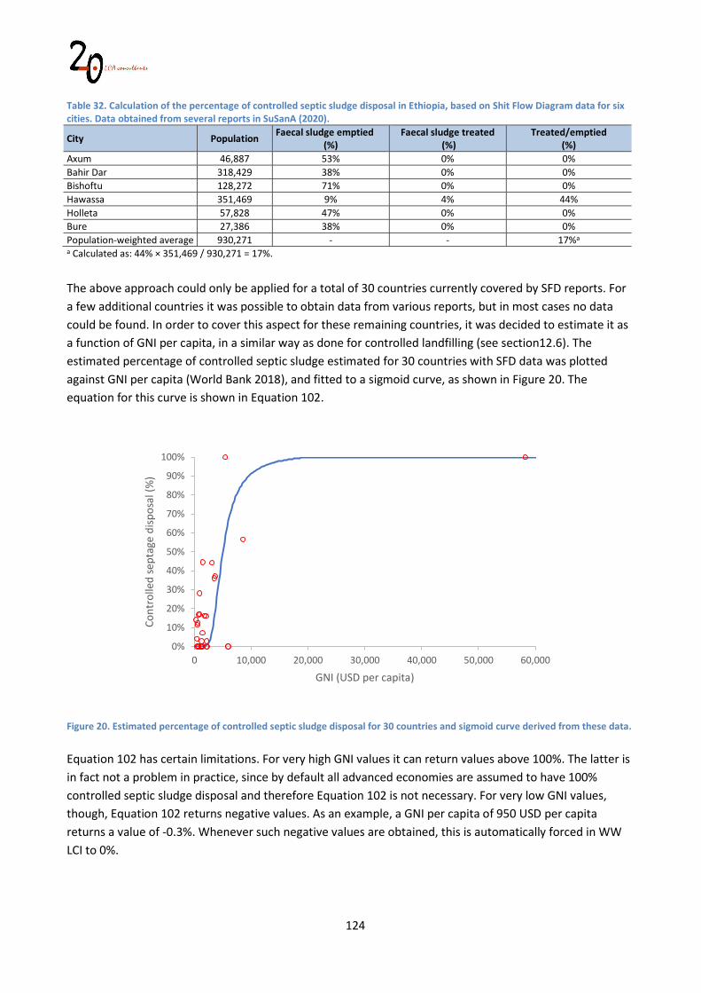
124

Table 32. Calculation of the percentage of controlled septic sludge disposal in Ethiopia, based on Shit Flow Diagram data for six cities. Data obtained from several reports in SuSanA (2020).

City Population Faecal sludge emptied (%)

Faecal sludge treated (%)

Treated/emptied (%)

Axum 46,887 53% 0% 0% Bahir Dar 318,429 38% 0% 0% Bishoftu 128,272 71% 0% 0% Hawassa 351,469 9% 4% 44% Holleta 57,828 47% 0% 0% Bure 27,386 38% 0% 0% Population-weighted average 930,271 - - 17%a

a Calculated as: 44% × 351,469 / 930,271 = 17%.

The above approach could only be applied for a total of 30 countries currently covered by SFD reports. For a few additional countries it was possible to obtain data from various reports, but in most cases no data could be found. In order to cover this aspect for these remaining countries, it was decided to estimate it as a function of GNI per capita, in a similar way as done for controlled landfilling (see section12.6). The estimated percentage of controlled septic sludge estimated for 30 countries with SFD data was plotted against GNI per capita (World Bank 2018), and fitted to a sigmoid curve, as shown in Figure 20. The equation for this curve is shown in Equation 102.

Figure 20. Estimated percentage of controlled septic sludge disposal for 30 countries and sigmoid curve derived from these data. Equation 102 has certain limitations. For very high GNI values it can return values above 100%. The latter is in fact not a problem in practice, since by default all advanced economies are assumed to have 100% controlled septic sludge disposal and therefore Equation 102 is not necessary. For very low GNI values, though, Equation 102 returns negative values. As an example, a GNI per capita of 950 USD per capita returns a value of -0.3%. Whenever such negative values are obtained, this is automatically forced in WW LCI to 0%.

0%

10%

20%

30%

40%

50%

60%

70%

80%

90%

100%

0 10,000 20,000 30,000 40,000 50,000 60,000

Cont

rolle

d se

ptag

e di

spos

al (%

)

GNI (USD per capita)

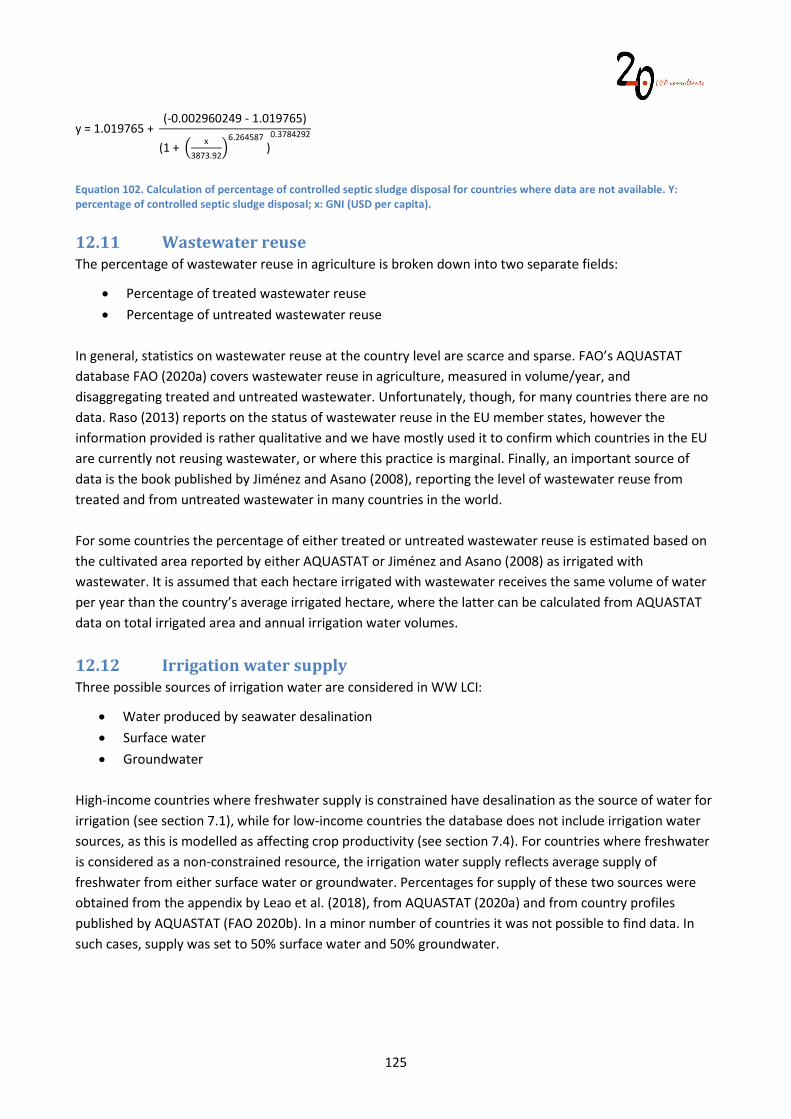
125

y = 1.019765 + (-0.002960249 - 1.019765)

(1 + x

3873.92

6.264587)0.3784292

Equation 102. Calculation of percentage of controlled septic sludge disposal for countries where data are not available. Y: percentage of controlled septic sludge disposal; x: GNI (USD per capita).

12.11 Wastewater reuse The percentage of wastewater reuse in agriculture is broken down into two separate fields:

Percentage of treated wastewater reuse Percentage of untreated wastewater reuse

In general, statistics on wastewater reuse at the country level are scarce and sparse. FAO’s AQUASTAT database FAO (2020a) covers wastewater reuse in agriculture, measured in volume/year, and disaggregating treated and untreated wastewater. Unfortunately, though, for many countries there are no data. Raso (2013) reports on the status of wastewater reuse in the EU member states, however the information provided is rather qualitative and we have mostly used it to confirm which countries in the EU are currently not reusing wastewater, or where this practice is marginal. Finally, an important source of data is the book published by Jiménez and Asano (2008), reporting the level of wastewater reuse from treated and from untreated wastewater in many countries in the world. For some countries the percentage of either treated or untreated wastewater reuse is estimated based on the cultivated area reported by either AQUASTAT or Jiménez and Asano (2008) as irrigated with wastewater. It is assumed that each hectare irrigated with wastewater receives the same volume of water per year than the country’s average irrigated hectare, where the latter can be calculated from AQUASTAT data on total irrigated area and annual irrigation water volumes.

12.12 Irrigation water supply Three possible sources of irrigation water are considered in WW LCI:

Water produced by seawater desalination Surface water Groundwater

High-income countries where freshwater supply is constrained have desalination as the source of water for irrigation (see section 7.1), while for low-income countries the database does not include irrigation water sources, as this is modelled as affecting crop productivity (see section 7.4). For countries where freshwater is considered as a non-constrained resource, the irrigation water supply reflects average supply of freshwater from either surface water or groundwater. Percentages for supply of these two sources were obtained from the appendix by Leao et al. (2018), from AQUASTAT (2020a) and from country profiles published by AQUASTAT (FAO 2020b). In a minor number of countries it was not possible to find data. In such cases, supply was set to 50% surface water and 50% groundwater.

126

12.13 Crop production A crop production mix is only defined in the database for those countries with a constrained freshwater supply and a GNI per capita below 12,535 USD (see section 7.1). For all remaining countries no crop mix is defined. The data sources used to define these crop mixes have been described in detail in sections 7.4.2 and 7.4.3.

12.14 Secondary wastewater treatment technology WW LCI addresses two types of WWTPs with secondary treatment, regarding the type of secondary treatment technology:

Activated sludge (see section 3.3). Waste stabilization ponds (see section 3.5).

The database provides a secondary treatment mix, with a percentage of wastewater treated by activated sludge and the remainder by stabilization ponds. It must be highlighted that this mix does not affect WWTPs with tertiary treatment, which are assumed in the model to use activated sludge only. In practice, though, many countries include other types of secondary treatment, such as trickling filters, upflow anaerobic sludge blanket (UASB), aerated lagoons, etc., however WW LCI does not currently cover these technologies. Whenever these technologies are reported, they are approximated in the model as activated sludge. The search for data on this subject has been done independently for each country, and sources are various. Very often, though, the same sources used to define wastewater collection and treatment (see section 12.1) as well as WWTP capacity (see section 12.5) are used here.

12.15 Stabilization pond capacity This field in the database reports the average capacity, in m3/day, of WWTPs applying this treatment technology. In WW LCI, the size of the stabilization pond affects the inputs of infrastructure materials, as described in section 3.5.2. The data used to complete this field originates in various reports and studies, often the same used to define the secondary wastewater treatment technology (section 12.14).

12.16 Primary wastewater treatment technology WW LCI addresses two types of WWTPs with primary treatment, regarding the type of primary treatment technology:

Conventional (see section 3.6). Chemically enhanced (see section 3.7).

The database provides a primary treatment mix, with a percentage of wastewater treated by conventional primary settling tanks and the remainder by chemically-enhanced primary treatment plants. It must be highlighted that this mix does not affect WWTPs with secondary treatment or tertiary treatment, where primary treatment is assumed as a conventional primary settling in all cases. Many countries in the database do not report primary treatment capacity, based on the data on wastewater collection and treatment (see section 12.1) and in many developing countries there is no centralized treatment of wastewater, making it unnecessary to determine a primary treatment mix.

127

Wherever primary treatment capacity is reported but no data are available to determine the treatment technology, this is assumed as 100% chemically-enhanced for advanced economies and 100% conventional for emerging and developing economies as defined by the IMF (2020).

128

References

Agriculture Canada (1975). Soil and air temperatures at Ottawa. Publication 1541 1975. Canada Department of Agriculture, Ottawa, K1A 0C7.

Ahn J H, Kim S, Park H, Rahm B, Pagilla K, Chandran K (2010) N2O Emissions from Activated Sludge Processes, 2008-2009: Results of a National Monitoring Survey in the United States. Environ. Sci. Technol. 2010, 44, 4505–4511.

Albadelejo A, Martínez J L, Santos J M (2017) Parametrización del consumo energético en las depuradoras de aguas residuales urbanas de la Comunidad Valenciana. Tecnoacqua. https://www.tecnoaqua.es/articulos/20170919/articulo-tecnico-parametrizacion-consumo-energetico-depuradoras-agua-residuales-urbanas-comunidad-valenciana#.WrS_jJdG0dV (accessed 8 November 2017).

Andersen HR, Kjølholt J, Hansen M, et al (2004) Degradation of estrogens in sewage treatment processes. Environ. Proj. no. 899:38.

Andreoli CV, Von Sperling M, Fernandes F (2007) Sludge treatment and disposal. In: Biological Wastewater Treatment Series, vol 6. IWA Publishing, Alliance House, 12 Caxton Street, London SW1H 0QS, UK.

AQUASTAT (2014) Water from the clouds. http://www.fao.org/3/I9253EN/i9253en.pdf (accessed 6/09/2020)

AQUASTAT (2018) Municipal wastewater production, collection, treatment and use. http://www.fao.org/nr/water/aquastat/wastewater/index.stm (accessed 8 November 2018).

Benth BL, Middlebrooks E J, Dennis B G, Reynolds JH (1981) Evaluation of Wastewater Filtration. Reports. Utah Water Research Laboratory. Paper 606. https://digitalcommons.usu.edu/water_rep/606 (accessed 6 November2018).

Buswell AM, Müller HF (1952) Mechanism of methane fermentation. Industrial and Engineering Chemistry, 44 (3): 550-552.

Cecchini G, Cirello P, Eramo B (2015) Partitioning dynamics and fate of metals in an urban wastewater treatment plant. Environmental Engineering and Management Journal,14 (7), 1511-1520.

Chai C, Zhang D, Yu Y, Feng Y, Wong M S (2015) Carbon Footprint Analyses of Mainstream Wastewater Treatment Technologies under Different Sludge Treatment Scenarios in China. Water, 7: 918-938.

Chaosakul T, Koottatep T, Polprasert C (2014) A model for methane production in sewers. Journal of Environmental Science and Health, Part A: Toxic/Hazardous Substances and Environmental Engineering, 49 (11): 1316-1321.

CIESIN (2012) National Aggregates of Geospatial Data: Population, Landscape and Climate Estimates Version 3 (PLACE III), Palisades, NY: NASA Socioeconomic Data and Applications Center (SEDAC). Center for International Earth Science Information Network (CIESIN), Columbia University, 2012. http://sedac.ciesin.columbia.edu/data/set/nagdc-population-landscape-climate-estimates-v3 (accessed 18/10/2020).

129

City of San Diego (2005) 2004 Annual Reports and Summary - Point Loma Wastewater Treatment Plant & Ocean Outfall. Environmental Monitoring and Technical Services Division, Public Utilities, San Diego, CA. https://www.sandiego.gov/sites/default/files/legacy/mwwd/pdf/pm/2004_2_inf_eff.pdf (accessed 24/04/2020).

City of San Diego (2008) 2007 Annual Reports and Summary - Point Loma Wastewater Treatment Plant & Ocean Outfall. Environmental Monitoring and Technical Services Division, Public Utilities, San Diego, CA. https://www.sandiego.gov/sites/default/files/legacy/mwwd/pdf/pm/2007influenteffluent.pdf (accessed 24/04/2020).

City of San Diego (2016) 2015 Annual Reports and Summary - Point Loma Wastewater Treatment Plant & Ocean Outfall. Environmental Monitoring and Technical Services Division, Public Utilities, San Diego, CA. https://www.sandiego.gov/sites/default/files/plwtp_annual_2016.pdf (accessed 24/04/2020).

Consequential-LCA (2015). Not fully utilised by-product. Last updated: 2015-10-27. https://consequential-lca.org/clca/by-products-recycling-and-waste/not-fully-utilised-by-product/ (accessed 04/04/2020).

COWI (2004) The FEASIBLE Model, Version 2. User Manual and Documentation, Appendix 3: Documentation of Expenditure Functions – Wastewater. https://www.oecd.org/env/outreach/methodologyandfeasiblecomputermodel.htm (accessed 21/04/2020).

CUAS (2015) Standard method and online tool for assessing and improving the energy efficiency of waste water treatment plants, Deliverable 2.1 - Study of published energy data. Version 1, prepared by Cologne University of Applied Sciences (CUAS).

Dalemo M, Sonesson U, Björklund A, Mingarini K, Frostell B, Jönsson H, Nybrant T, Sundqvist J-O, Thyselius L (1997b) ORWARE – A simulation model for organic waste handling systems. Part 1: Model description. Resources, Conservation and Recycling 21: 17-37.

Delft University of Technology (2013) Wastewater treatment - lecture notes. Faculty of Civil Engineering and Geosciences, Department of Water Management, Section of Sanitary Engineering.

Doblado J (2004) Estudio de las tecnologías de secado de biosólidos procedentes de EDAR. Proyecto fin de carrera, Departamento de Ingeniería Energética y Mecánica de Fluidos, Escuela Superior de Ingenieros, Universidad de Sevilla.

Doka, G. (2007) Life Cycle Inventories of Waste Treatment Services. Final report ecoinvent 2000 No. 13, EMPA St. Gallen, Swiss Centre for Life Cycle Inventories, Duebendorf, Switzerland.

Domènech X (2020) Personal communication with Prof. Xavier Domènech, Department of Chemistry, Universitat Autònoma de Barcelona (02/06/2020).

Doorn M (2018) Communication by email with Michiel R. J. Doorn, Director, Ecoawareness, on the 8 April 2018.

Doorn MRJ, Liles DS (1999) Quantification of Methane Emission and Discussion of Nitrous Oxid, and Ammonia Emissions from Septic Tanks, Latrines, and Stagnant Open Sewers in the World.Prepared for the USEPA. EPA-600/R-99-089.

130

Doorn MRJ, Towprayoon S, Manso Vieira SM, Irving W, Palmer C, Pipatti R, Wang C (2006) Wastewater treatment and discharge. In: Eggleston HS, Buendia L, Miwa K, Ngara T, Tanabe K (eds) IPCC guidelines for national greenhouse gas inventories, vol 5. IGES, Hayama, Chapter 6.

Droste R L (1997). Theory and Practice of Water and Wastewater treatment, John Wiley and Sons, Inc.

Eijo-Río E, Petit-Boix A, Villalba G, Suárez-Ojeda ME, Marin D, Amores MJ, Aldea X, Rieradevall J, Gabarrell X (2015) Municipal sewer networks as sources of nitrous oxide, methane and hydrogen sulphide emissions: A review and case studies. Journal of Environmental Chemical Engineering, 3 (3): 2084-2094.

Environmental Commissioner of Ontario (2017) Every Drop Counts. Reducing the Energy and Climate Footprint of Ontario’s Water Use. http://docs.assets.eco.on.ca/reports/energy/2016-2017/Every-Drop-Counts.pdf (accessed 14 November 2018)

ERG (2011) Opportunities for Combined Heat and Power at Wastewater Treatment Facilities: Market Analysis and Lessons from the Field. Report prepared by: Eastern Research Group, Inc. (ERG) and Resource Dynamics Corporation (RDC) for the U.S. Environmental Protection Agency, Combined Heat and Power Partnership, October 2011.

EurObserv’ER (2017) Biogas barometer 2017. https://www.eurobserv-er.org/category/all-biogas-barometers/ (accessed 14 November 2018).

European Environment Agency (2017) Waterbase - UWWTD: Urban Waste Water Treatment Directive – reported data. https://www.eea.europa.eu/data-and-maps/data/waterbase-uwwtd-urban-waste-water-treatment-directive-5#tab-european-data (accessed 7 November 2018)

EUROSTAT (2018a) Generation and discharge of wastewater in volume [env_ww_genv]. Urban wastewater generated - total. WW_GTD. http://appsso.eurostat.ec.europa.eu/nui/show.do?dataset=env_ww_genv&lang=en (accessed 8 November 2018).

EUROSTAT (2018b) Sewage sludge production and disposal [env_ww_spd]. https://ec.europa.eu/eurostat/data/database?node_code=env_ww_spd (Accessed 14 November 2018)

EUROSTAT (2020) Population connected to wastewater treatment plants. https://appsso.eurostat.ec.europa.eu/nui/show.do?dataset=env_ww_con&lang=en (accessed 11/10/2020)

FAO (2020a) AQUASTAT. http://www.fao.org/nr/water/aquastat/data/query/index.html?lang=es (accessed 2/11/2020)

FAO (2020b) Country profiles. http://www.fao.org/aquastat/en/countries-and-basins/country-profiles (accessed 7/11/2020)

FAO & IFA (2001) Global estimates of gaseous emissions of NH3, NO and N2O from agricultural land. Food and Agriculture Organization of the United Nations (FAO) and International Fertilizer Industry Association (IFA). Rome.

Feachem, RG, Bradley, DJ, Garelick H, Duncan Mara D. (1983) Sanitation and disease : health aspects of excreta and wastewater management.World Bank Studies in Water Supply and Sanitation 3. John Wiley and Sons, Bath, UK.

131

Foley J, de Haas D, Hartley K, Lant P (2010) Comprehensive life cycle inventories of alternative wastewater treatment systems. Water Research 44 (2010) 1654 – 1666.

Frischknecht R, Jungbluth N, Althaus H-J, Doka G, Dones R, Hischier R, Hellweg S, Nemecek T, Rebitzer G, Spielmann M (2007) Overview and Methodology. Final report ecoinvent data v2.0, No. 1. Swiss Centre for Life Cycle Inventories, Dübendorf, CH.

GET.invest (2019) Senegal: Renewable Energy in Agricultural Value Chains. https://www.get-invest.eu/wp-content/uploads/2019/06/GETinvest-Market-Insights_SEN_PV_MBC-Small-scale_2019.pdf (accessed 8 August 2020)

Gikas GD, Tsihrintzis VA (2014) Stabilization pond systems for wastewater treatment: facility costs and environmental footprint assessment. Global NEST Journal, Vol 16, No 2, pp 375-385.

Graham J, Polizzotto M (2013) Pit Latrines and Their Impacts on Groundwater Quality: A Systematic Review. Environ. Health Perspect. 121: 521−530.

Griffith DR, Barnes RT, Raymond PA (2009) Inputs of Fossil Carbon from Wastewater Treatment Plants to U.S. Rivers and Oceans. Environ. Sci. Technol., 2009, 43 (15): 5647–5651.

Guisasola A, de Haas D, Keller J, Yuan Z (2008) Methane formation in sewer systems. Wat Res, 42: 1421 – 1430.

Handa D, Frazier RS, Taghvaeian S, Warren JG (2018) The Efficiencies, Environmental Impacts and Economics of Energy Consumption for Groundwater-Based Irrigation in Oklahoma. Agriculture, 9, 27.

Hansen TL, Bhander GS, Christensen TH, Bruun S, Jensen LS (2006) Life cycle modelling of environmental impacts of application of processed organic municipal solid waste on agricultural land (EASEWASTE). Waste Management & Research, 24, 153.

Hartung H, Pluschke L (2018) The benefits and risks of solar-powered irrigation - a global overview. Published bythe Food and Agriculture Organization of the United Nations and Deutsche Gesellschaft für Internationale Zusammenarbeit. ISBN 978-92-5-130479-2.

Hauschild M, Potting J (2005) Spatial differentiation in Life Cycle impact assessment - The EDIP2003 methodology. Environmentla News nº 80 2005, Danish Ministry of the Environment.

Henze M, Comeau Y (2008) Wastewater characterization. In: Henze M et al. (Ed.). Biological Wastewater Treatment: Principles Modelling and Design. Published by IWA Publishing, London, UK. Chapter 3.

Hernandez-Paniagua IH, Ramirez-Vargas R, Ramos-Gomez MS, Dendooven L, Avelar-Gonzalez FJ, Thalasso F (2013) Greenhouse gas emissions from stabilization ponds in subtropical climate. Environmental Technology, DOI: 10.1080/09593330.2013.848910.

IEA (2017) IEA Bioenergy Task 37 Country Report Summaries 2017. http://task37.ieabioenergy.com/country-reports.html?file=files/daten-redaktion/download/publications/country-reports/Summary/IEA%20Bioer%20T37CRS%202017_Final.pdf (accessed 14 November 2018)

IFASTAT (2019) https://www.ifastat.org/databases/plant-nutrition (accessed 10/01/2019).

132

IMF (2020) Country Composition of WEO Groups. https://www.imf.org/external/pubs/ft/weo/2020/02/weodata/groups.htm#ae (accessed 30/10/2020)

InfraCo Africa (2019) Senegal: Bonergie Irrigation - Expanding access to solar powered irrigation technology. https://infracoafrica.com/project/bonergie-irrigation-i/ (accessed 8 August 2020)

IPCC (2006) IPCC Guidelines for National Greenhouse Gas Inventories. Vol. 5, Waste, Chapter 4 biological treatment of solid waste. IGES, Japan.

IPCC (2006b) 2006 IPCC Guidelines for National Greenhouse Gas Inventories, Volume 4 - Agriculture, Forestry and Other Land Use. Prepared by the National Greenhouse Gas Inventories Programme. IGES, Japan.

Isgren M, Mårtensson P (2013) Methane formation in sewer systems. Master Thesis, Department of Chemical Engineering, Lund University, Sweden.

Jiménez B, Asano T (2008) Water reuse. An International Survey of current practice, issues and needs. IWA Publishing.

Jönsson H, Baky A, Jeppsson U, Hellström D, Kärrman E (2005) Composition of urine, faeces, greywater and biowaste for utilisation in the URWARE model. Dept. of Industrial Electrical Engineering and Automation, Lund University, CHALMERS UNIVERSITY OF TECHNOLOGY, Gothenburg, Sweden.

Kalbar P, Muñoz I, Birkved M (2018) WW LCI v2: a second-generation life cycle inventory model for chemicals discharged to wastewater systems. Sci Total Environ, 622–623: 1649-1657.

Kampman B et al. (2016) Optimal use of biogas from waste streams. An assessment of the potential of biogas from digestion in the EU beyond 2020. Prepared for the European Commission.

Kampschreur M J, Temmink H, Kleerebezem R, Jetten M S M, van Loosdrecht M C M (2009) Nitrous oxide emission during wastewater treatment. Water Research, 43 (17): 4093-4103.

Kingsley OC (2011) Using Life Cycle Assessment (LCA) to Assess the Sustainability of Urban Wastewater Treatment Systems: a Case Study of the Wastewater Treatment Technology of the Bogotá River. Trabajo de grado presentado para optar al título de Maestria en Ingeniería - Ingeniería Ambiental. Universidad Nacional de Colombia, Bogotá.

Law Y, Jacobsen GE, Smith AM, Yuan Z, Lant P (2013) Fossil organic carbon in wastewater and its fate in treatment plants. Water Research, 47 (14): 5270-5281.

Law Y, Ye L, Pan Y, Yuan Z (2012) Nitrous oxide emissions from wastewater treatment processes. Phil. Trans. R. Soc. B, 367: 1265–1277.

Leao S, Roux P, Núñez M, Loiseau E, Junqua G, Sferratore A, Penru Y, Rosenbaum R K (2018) A worldwide-regionalised water supply mix (WSmix) for life cycle inventory of water use. Journal of Cleaner Production 172, 302-313.

Leverentz HL, Tchobanoglous G, Darby J (2010) Evaluation of Greenhouse Gas Emissions from Septic Systems. Water Environment Research Foundation & IWA Publishing.

Liu (2015) Measurement and understanding of methane emission from sewers. PhD Thesis, University of Queensland, School of Chemical Engineering.

133

Magar KTK (2016) Comparative environmental performance of small scale wastewater treatment systems in Norway – life cycle analysis. MSc Thesis, Norwegian University of Life Science, Faculty of Environmental Science and Technology, Department of Environmental Science. https://brage.bibsys.no/xmlui/handle/11250/2449011 (accessed 14 November 2018).

Mayo AW (2013) Nitrogen mass balance in waste s.tabilization ponds at the University of Dar es Salaam, Tanzania. African Journal of Environmental Science and Technology, Vol. 7(8), pp. 836-845, August 2013.

Metcalf & Eddy (2000) Ingenieria de aguas residuales, Tratamiento, vertido y reutilización. McGraw-Hill.

Metcalf E, Asano T, Burton F, Leverenz H, Tsuchihashi R, Tchobanoglous G (2007) Water Reuse: Issues, Technologies, and Applications. Metcalf & Eddy, Inc.

Methanol Institute (2018) Wastewater treatment. https://www.methanol.org/wastewater-treatment/ (accessed 16 November 2018).

Morera S (2016) Comprehensive inventories for life cycle assessment in wastewater systems. PhD thesis, Universitat de Girona. https://www.tdx.cat/handle/10803/363226 (accessed 22/04/2020)

Morera S, Corominas L, Rigola M, Poch M, Comas J (2017) Using a detailed inventory of a large wastewater treatment plant to estimate the relative importance of construction to the overall environmental impacts. Water Research 122: 614-623.

Muñoz I, Milà I Canals L, Clift R, Doka G (2007) A simple model to include human excretion and wastewater treatment in life cycle assessment of food products. CES Working Paper 01/07, Centre for Environmental Strategy, University of Surrey.

Muñoz I, Milà-i-Canals L, Fernández-Alba AR (2010) Life cycle assessment of water supply plans in Mediterranean Spain. J. Ind. Ecol. 14, 902–918.

Muñoz I, Otte N, Van Hoof G, Rigarlsford G (2017) A model and tool to calculate life cycle inventories of chemicals discharged down the drain. International Journal of Life Cycle Assessment, 22(6), 986-1004.

Muñoz I, Rigarlsford G, Milà i Canals L, King H (2013) Accounting for greenhouse-gas emissions from the degradation of chemicals in the environment. International Journal of Life Cycle Assessment, 18 (1): 252-262.

Muñoz, I (2017) Consequential LCI modeling of chemicals in wastewater: including avoided nutrient treatment. SETAC Europe 28th Annual Meeting, Barcelona, 27-28 November 2017.

Nemecek T, Kägi T (2007) Life cycle inventories of agricultural production systems. Ecoinvent report no 15. Swiss Centre for Life Cycle Inventories, Dubendorf, Switzerland.

OECD.Stat (2020) Wastewater treatment (% population connected). https://stats.oecd.org/viewhtml.aspx?datasetcode=WATER_TREAT&lang=en (Accessed 11/10/2020).

Outotec (2020) Sustainable sewage sludge incineration for Zürich Canton. https://www.outotec.com/references/sustainable-sewage-sludge-incineration-for-zurich-canton/ (accessed 15/12/2020).

134

Paing, J., Sambuco, J.-P., Costa, R., Rambaud, A. & Picot, B. (2003). Bilan du carbone dans le lagunage anaérobie appliqué sous climat méditerranéen. Revue des sciences de l'eau / Journal of Water Science, 16 (3), 357–368. https://doi.org/10.7202/705512ar

Paredes MG, Güereca LP, Molina LT, Noyola A (2015) Methane emissions from stabilization ponds for municipal wastewater treatment in Mexico, Journal of Integrative Environmental Sciences, 12:sup1, 139-153, DOI: 10.1080/1943815X.2015.1110185.

Paul E, Laval M L, Sperandio M. (2001) Excess sludge production and costs due to phosphorus removal. Environ Technol. 22(11):1363-71.

Perchard E (2016) Austerity-hit Greece faces further fines for poor waste management. Resource. https://resource.co/article/austerity-hit-greece-faces-further-fines-poor-waste-management-11368 (accessed 9 November 2018).

Picot B, Sambuco JP, Brouillet JL, Riviere Y (2005) Wastewater stabilisation ponds: sludge accumulation, technical and financial study on desludging and sludge disposal case studies in France. Water Science & Technology Vol 51 No 12 pp 227–234.

Pipatti R, Svardal P, Alves JWS, Gao Q, Cabrera CL, Mareckova K, Oonk H, Scheehle E, Sharma C, Smith A, Yamada M (2006) Chapter 3: Solid waste disposal. In: Eggleston HS, Buendia L, Miwa K, Ngara T, Tanabe K (eds) IPCC guidelines for national greenhouse gas inventories, vol 5: Waste. IGES, Hayama, Chapter 6.

Poulsen TG, Hansen J A (2003) Strategic environmental assessment of alternative sewage sludge management scenarios. Waste Manag Res, 21: 19–28. doi: 10.1177/0734242X0302100103

Qasim, S.R. (1999) Wastewater treatment plants: planning, design, and operation. CRC Press.

Raso J (2013) UPDATED REPORT ON WASTEWATER REUSE IN THE EUROPEAN UNION. Service contract for the support to the follow-up of the Communication on Water Scarcity and Drougths. https://ec.europa.eu/environment/water/blueprint/pdf/Final%20Report_Water%20Reuse_April%202013.pdf (accessed 2/11/2020)

Reid MC, Guan K, Wagner F, Mauzerall DL (2014) Global Methane Emissions from Pit Latrines. Environ. Sci. Technol., 48, 8727−8734.

Reuters (2014) EU Court fines Italy record 40 million euros for illegal waste. https://www.reuters.com/article/us-italy-environment/eu-court-fines-italy-record-40-million-euros-for-illegal-waste-idUSKCN0JG1AJ20141202 (accessed 9 November 2018).

Revuelta I (2017) Condena de la justicia europea a España por los vertederos ilegales. In English: European Courts rule against Spain on illegal landfills.https://www.residuosprofesional.com/condena-a-espana-vertederos-ilegales/ (accessed 9 November 2018)

Saudi Arabian Water Environment Association (2013) Wastewater sludge treatment and disposal in KSA. http://www.sawea.org/pdf/waterarabia2013/Sesssion_C/WASTEWATER_SLUDGE_TREATMENT_AND_DISPOSAL%20IN%20KSA.pdf (accessed 14 Novmeber 2018)

Schmid F (2008) Sewage water: interesting heat source for heat pumps and chiller. Conference Proceedings Paper. IEA Heat Pump Conference 2008, Zurich, Switzerland.

135

Smidt SJ, Haacker EMK, Kendall AD, Deines JM, Pei L, Cotterman KA, Li H, Liu X, Basso B, Hyndman DW (2016) Complex water management in modern agriculture: Trends in the water-energy-food nexus over the High Plains Aquifer. Science of The Total Environment, 566–5676: 988-1001.

Sonesson U (1996) Modelling of the compost and transport process in the ORWARE simulation model. Swedish University of Agricultural Sciences, Uppsala.

Sonnemann G and Vigon B (eds.) (2011), Global Guidance Principles for Life Cycle Assessment Databases. UNEP SETAC Life Cycle Initiative. http://www.unep.fr/shared/publications/pdf/DTIx1410xPA-GlobalGuidancePrinciplesforLCA.pdf (accessed 10 April 2017)

Stillwell A S, Hoppock D C, Webber M E (2010) Energy Recovery from Wastewater Treatment Plants in the United States: A Case Study of the Energy-Water Nexus. Sustainability 2010, 2, 945-962.

Stuer-Lauridsen F, Birkved M, Hansen LP, et al (2000) Environmental risk assessment of human pharmaceuticals in Denmark after normal therapeutic use. Chemosphere 40:783–793.

SuSanA (2020) SFD Promotion Initiative. Worldwide projects. https://sfd.susana.org/about/worldwide-projects (accessed 30/10/2020)

Taylor K (2018) Faecal Sludge and Septage Treatment: A guide for low and middle income countries. Rugby, UK, Practical Action Publishing, http://dx.doi.org/10.3362/ 9781780449869.

Tilley E, Ulrich L, Lüthi C, Reymond Ph, Zurbrügg C (2014) Compendium of Sanitation Systems and Technologies (2 ed.). Dübendorf, Switzerland: Swiss Federal Institute of Aquatic Science and Technology (Eawag). ISBN 978-3-906484-57-0.

Trapote A, Albadalejo A, Simón P (2014) Energy consumption in an urban wastewater treatment plant: the case of Murcia Region (Spain). Civil Engineering and Environmental Systems, 31 (4): 304-310.

Turovskiy I S, Mathai PK (2006) Wastewater Sludge Processing. John Wiley & Sons, New Jersey.

UN News (2019) ‘Transformational benefits’ of ending outdoor defecation: Why toilets matter. https://news.un.org/en/story/2019/11/1051561 (accessed 7/05/2020).

USEPA (2018) Clean Watersheds Needs Survey. https://www.epa.gov/cwns (accessed 16 November 2018)

Van Zelm R, Huijbregts M A J, van de Meent D (2009) USES-LCA 2.0—a global nested multi-media fate, exposure, and effects model. Int J Life Cycle Assess, 14:282–284.

Vasyd (2016) Sjölunda wastewater treatment plant. https://www.vasyd.se/-/media/Documents/Informationsmaterial/Vatten-och-avlopp/Avloppsreningsverk-och-skyddsinformation/SjolundaReningsverkEnglish201609Webb.pdf (accessed 25/03/2020).

Von Sperling M (2007a) (ed). Biological wastewater treatment series. Vol 2: Basic principles of wastewater treatment. IWA Publishing, London.

Von Sperling M (2007b)(ed).Biological wastewater treatment series. Vol 5: Activated sludge and aerobic biofilm reactors. IWA Publishing, London.

Von Sperling M (2007c) (ed). Biological wastewater treatment series. Vol 1: Wastewater characteristics, treatment and disposal. IWA Publishing, London.

136

Von Sperling M (2016) Urban wastewater treatment in Brazil. Interamerican Development Bank. https://publications.iadb.org/bitstream/handle/11319/7783/Urban-wastewater-treatment-in-Brazil.pdf?sequence=1&isAllowed=y (accessed 18/04/2020).

Wang J, Conway D, Zhang L, Xiong W (2012) China's water–energy nexus: Greenhouse-gas emissions from groundwater use for agriculture. Environ. Res. Lett. 7, 014035.

Wason SK (2006) Cogeneration Technologies, Trends for Wastewater Treatment Facilities. WaterWorld ,vol 22, issue 6. https://www.waterworld.com/articles/print/volume-22/issue-6/editorial-focus/cogeneration-technologies-trends-for-wastewater-treatment-facilities.html (accessed 13 november 2018)

Weatherbase (2020) https://www.weatherbase.com/weather/countryall.php3 (accessed 7 November 2018).

Weidema B P (2014) Example –marginal water supply in Israel. Version: 2015-06-11 www.consequential-lca.org (accessed 1 August 2020).

Weidema B P, Ekvall T, Heijungs R (2009), Guidelines for applications of deepened and broadened LCA. Deliverable D18 of work package 5 of the CALCAS project. http://fr1.estis.net/includes/file.asp?site=calcas&file=7F2938F9-09CD-409F-9D70-767169EC8AA9 (accessed 10 April 2017).

Weidema BP (1998) Multi-User Test of the Data Quality Matrix for Product Life Cycle Inventory. The International Journal of Life Cycle Assessment 3(5): 259-265.

Weidema BP (2003), Market information in life cycle assessment. Environmental project nr. 863. Danish EPA.

Weidema BP, Bauer C, Hischier R, Mutel C, Nemecek T, Reinhard J, Vadenbo CO, Wernet G (2013). Overview and methodology. Data quality guideline for the ecoinvent database version 3. Ecoinvent Report 1(v3). St. Gallen: The ecoinvent Centre.

Weidema BP, Wesnaes MS (1996) Data quality management for life cycle inventories - an example of using data quality indicators. Journal of Cleaner Production, 4(3-4): 167-174.

WHO-UNICEF (2019) Estimates on the use of water, sanitation and hygiene by country (2000-2017). Joint Monitoring Programme for Water Supply, Sanitation and Hygiene. https://washdata.org/data (accessed 11/10/2020).

Wikipedia (2018) Chemical oxygen demand. https://en.wikipedia.org/wiki/Chemical_oxygen_demand (Accessed 13 November 2018).

Willis J, Checkel D, Handford D, Shah A, Joiner M (2013) Flare efficiency estimator and case studies. Water Environment Research Foundation, WERF. Report U2R08d. https://www.nyserda.ny.gov/-/media/Files/EERP/Commercial/Sector/Municipal-Water-Wastewater-Facilities/flare-efficiency-estimator.pdf (accessed 21 November 2018).

Winrock (2008) Feasibility study for developing proposal under clean development mechanism (CDM) for claiming carbon credits for leach pit toilets & toilet linked biogas plants. Final report. Prepared by Winrock International India

137

World Bank (2018) World Development Indicators. http://databank.worldbank.org/data/reports.aspx?source=world-development-indicators# (Accessed 12 november 2018)

World Bank (2019b) People practicing open defecation (% of population). https://data.worldbank.org/indicator/SH.STA.ODFC.ZS (accessed 25/10/2020).

World Bank (2020a) Average precipitation in depth (mm per year). https://data.worldbank.org/indicator/AG.LND.PRCP.MM (accessed 07/05/2020).

World Bank (2020b) World Bank Country and Lending Groups. https://datahelpdesk.worldbank.org/knowledgebase/articles/906519#High_income (accessed 1 August 2020)

WRI (2019) Aqueduct 3.0 Country Rankings. World Resources Institute. https://www.wri.org/applications/aqueduct/country-rankings/ (accessed 1 August 2020).

Yacob TW, Fisher R, Linden KG, Weimer AW (2018) Pyrolysis of human feces: Gas yield analysis and kinetic modeling. Waste Management, 79: 214–222.

Yoshida H, Christensen TH, Guildal T, Scheutz C (2015) A comprehensive substance flow analysis of a municipal wastewater and sludge treatment plant. Chemosphere, 138: 874–882.

Yr (2018) Weather statistics for Zurich, Zürich (Switzerland. https://www.yr.no/place/Switzerland/Z%C3%BCrich/Zurich/statistics.html (accessed 13 November 2018).

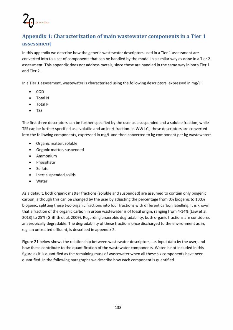
138

Appendix 1: Characterization of main wastewater components in a Tier 1 assessment

In this appendix we describe how the generic wastewater descriptors used in a Tier 1 assessment are converted into to a set of components that can be handled by the model in a similar way as done in a Tier 2 assessment. This appendix does not address metals, since these are handled in the same way in both Tier 1 and Tier 2. In a Tier 1 assessment, wastewater is characterized using the following descriptors, expressed in mg/L:

COD Total N Total P TSS

The first three descriptors can be further specified by the user as a suspended and a soluble fraction, while TSS can be further specified as a volatile and an inert fraction. In WW LCI, these descriptors are converted into the following components, expressed in mg/L and then converted to kg component per kg wastewater:

Organic matter, soluble Organic matter, suspended Ammonium Phosphate Sulfate Inert suspended solids Water

As a default, both organic matter fractions (soluble and suspended) are assumed to contain only biogenic carbon, although this can be changed by the user by adjusting the percentage from 0% biogenic to 100% biogenic, splitting these two organic fractions into four fractions with different carbon labelling. It is known that a fraction of the organic carbon in urban wastewater is of fossil origin, ranging from 4-14% (Law et al. 2013) to 25% (Griffith et al. 2009). Regarding anaerobic degradability, both organic fractions are considered anaerobically degradable. The degradability of these fractions once discharged to the environment as in, e.g. an untreated effluent, is described in appendix 2. Figure 21 below shows the relationship between wastewater descriptors, i.e. input data by the user, and how these contribute to the quantification of the wastewater components. Water is not included in this figure as it is quantified as the remaining mass of wastewater when all these six components have been quantified. In the following paragraphs we describe how each component is quantified.

139

Figure 21. Relationship between wastewater descriptors (input data) and wastewater components in a Tier 1 assessment in WW LCI.

A1.1 Organic matter, soluble Soluble organic matter is specified in WW LCI with the generic formula CaHbOc. C in this formula corresponds to the amount of soluble organic carbon (Csol), which is calculated in mg/L based on the amount of soluble COD (CODsol) with Equation 103:

Csol = CODsol 2.75

Equation 103. Calculation of Csol. Where 2.75 is the average ratio of COD to total organic carbon in urban wastewater, based on Henze and Comeau (2008). CODsol can be directly specified by the user as input data (CODsol,in), otherwise it is estimated with either Equation 104 or Equation 105: CODsol = CODin – (TSSin · 0.8 · 1.406) Equation 104. Calculation of CODsol when the user specifies TSS. CODsol = CODin – (VSSin · 1.406) Equation 105. Calculation of CODsol when the user specifies VSS. Equation 104 is used when the user specifies only TSS, while Equation 105 is used instead when the user specifies VSS. CODin is the concentration of total COD specified by the user (mg/L), TSSin is the concentration of TSS specified by the user (mg/L), VSSin is the concentration of VSS specified by the user (mg/L), 0.8 is the average ratio of VSS to TSS in urban wastewater, based on Henze and Comeau. (2008) and 1.406 is the average ratio of suspended COD to VSS in urban wastewater, also based on Henze and Comeau (2008). The content in O and H in soluble organic matter (Osol, Hsol), in mg/L, is calculated with Equation 106 and Equation 107:

Soluble Suspended

Soluble Suspended

Soluble Suspended

Volatile Inert

Organic matter, soluble

Organic matter, suspended

Ammonium

Phosphate

Sulfate

Inert suspended solids

COD

Total N

Total P

TSS

140

Osol = (Csol · O/C) – (PO4 · 64/95) – (SO4 · 64/96) Equation 106. Calculation of Osol. Hsol = (Csol · H/C) – (NH4 · 4/18) Equation 107. Calculation of Hsol. Where O/C and H/C are the mass ratios of O and H to total organic carbon in wastewater, respectively, taken as 0.691 and 0.148, respectively, based on an analysis of human excreta by Yacob et al. (2018), PO4 is the calculated concentration, in mg/L, of phosphate present in wastewater (see Equation 133), SO4 is the calculated concentration, in mg/L, of sulfate present in wastewater (see Equation 135) and NH4 is the calculated concentration, in mg/L, of ammonium present in wastewater (see Equation 131). Once Csol, Osol and Hsol are quantified, their sum in mg/L equals the concentration of soluble organic matter in the defined wastewater. The subindexes a, b and c in the CaHbOc formula are obtained with the following equations: a = Csol / 12 Equation 108. Calculation of the ‘a’ subindex in the empirical formula CaHbOc for soluble organic matter. b = Hsol Equation 109. Calculation of the ‘b’ subindex in the empirical formula CaHbOc for soluble organic matter. c = Osol / 16 Equation 110. Calculation of the ‘c’ subindex in the empirical formula CaHbOc for soluble organic matter. The molecular weight (g/mol) considered for soluble organic matter is the sum of Csol, Osol and Hsol.

A1.2 Organic matter, suspended Suspended organic matter is specified in WW LCI with the generic formula CaHbOcNdSePf. C in this formula corresponds to the amount of suspended organic carbon (Csusp), which is calculated in mg/L with Equation 111: Csusp = VSS · 0.511 Equation 111. Calculation of Csusp. Where 0.511 is the average ratio of suspended organic carbon to volatile suspended solids in urban wastewater, based on Henze and Comeau (2008). VSS is in turn calculated with Equation 112:

141

VSS = CODsusp 1.406

Equation 112. Calculation of VSS. Where CODsusp is the suspended COD concentration, in mg/L. This parameter can be entered by the user if known (CODsusp,in), otherwise it is calculated with the following hierarchy of equations: CODsusp = CODin - CODsol

Equation 113. Calculation of CODsusp when the user specifies total COD (CODin). Equation 113 is applied when the user only specifies the total COD in wastewater (CODin). In this case CODsol is calculated with either Equation 104 or Equation 105. If the user has not specified CODin, then Equation 114 is used: CODsusp = VSSin · 1.406 Equation 114. Calculation of CODsusp when the user specifies VSS. Equation 114 is applied as a replacement for Equation 113, if the user specifies VSSin. If Equation 114 cannot be applied, then Equation 115 is used: CODsusp = CODsol,in + CODsusp,in - CODsol

Equation 115. Calculation of CODsusp when the user specifies COD . Where CODsol is calculated with either Equation 104 or Equation 105. The content in O and H in suspended organic matter (Osusp, Hsusp), in mg/L, is calculated with Equation 116 and Equation 117: Osusp = (Csusp · O/C) Equation 116. Calculation of Osusp. Hsusp = (Csusp · H/C) Equation 117. Calculation of Hsusp. The nitrogen content in suspended organic matter (Nsusp), in mg/L, can be specified by the user, otherwise it is calculated with Equation 118:

142

Nsusp = Nin · %Nsusp

Equation 118. Calculation of Nsusp. Where Nin is the concentration of total nitrogen specified by the user, in mg/L, and %Nsusp is the fraction of total nitrogen in suspended form, calculated with Equation 119: %Nsusp = 1 - %Nsol

Equation 119. Calculation of %Nsusp. Where %Nsol is the fraction of total nitrogen in soluble form, calculated in turn with Equation 120:

%Nsol = CODsol · 0.167

CODsol · 0.167 + VSS · 0.031 Equation 120. Calculation of %Nsol. Where 0.167 and 0.031 are the average ratios of soluble nitrogen to soluble COD and particulate nitrogen to VSS, respectively, both values based on Henze and Comeau (2008). The phosphorus content in suspended organic matter (Psusp), in mg/L, can be specified by the user, otherwise it is calculated with Equation 121: Psusp = Pin · %Psusp

Equation 121. Calculation of Psusp. Where Pin is the concentration of total phosphorus specified by the user, in mg/L, and %Psusp is the fraction of total phosphorus in suspended form, calculated with Equation 122: %Psusp = 1 - %Psol

Equation 122. Calculation of %Psusp. Where %Psol is the fraction of total phosphorus in soluble form, calculated in turn with Equation 123:

%Psol = CODsol · 0.033

CODsol · 0.033 + VSS · 0.016 Equation 123. Calculation of %Psol. Where 0.033 and 0.016 are the average ratios of soluble phosphorus to soluble COD and particulate phosphorus to VSS, respectively, both values based on Henze and Comeau (2008).

143

The sulfur content in suspended organic matter (Ssusp), in mg/L, is approximated based on the suspended nitrogen content in wastewater (Nsusp) by means of Equation 124:

Ssusp = Nsusp

10.55 Equation 124. Calculation of Ssusp. Where 10.55 is the ratio of total nitrogen to total sulphur in domestic wastewater according to Jönsson et al. 2005). Once Csusp, Osusp, Hsusp, Nsusp, Psusp and Ssusp are quantified, their sum in mg/L equals the concentration of suspended organic matter in the defined wastewater. The subindexes in the CaHbOcNdSePf formula are obtained with the following equations: a = Csusp / 12 Equation 125. Calculation of the ‘a’ subindex in the empirical formula CaHbOcNdSePf for suspended organic matter. b = Hsusp Equation 126. Calculation of the ‘b’ subindex in the empirical formula CaHbOcNdSePf for suspended organic matter. c = Osusp / 16 Equation 127. Calculation of the ‘c’ subindex in the empirical formula CaHbOcNdSePf for suspended organic matter. d = Nsusp / 14 Equation 128. Calculation of the ‘d’ subindex in the empirical formula CaHbOcNdSePf for suspended organic matter. e = Ssusp / 32 Equation 129. Calculation of the ‘e’ subindex in the empirical formula CaHbOcNdSePf for suspended organic matter. f = Psusp / 31 Equation 130. Calculation of the ‘f’ subindex in the empirical formula CaHbOcNdSePf for suspended organic matter. The molecular weight (g/mol) considered for suspended organic matter is the sum of Csusp, Osusp, Hsusp, Nsusp, Psusp and Ssusp.

A1.3 Ammonium The concentration of ammonium in wastewater (NH4), in mg/L, is calculated with Equation 131:

144

NH4 = Nsol · 18/14 Equation 131. Calculation of ammonium concentration in wastewater. Where Nsol is the soluble nitrogen concentration in wastewater, in mg/L. This parameter can be entered directly by the user when specifying the wastewater composition, otherwise it is calculated with Equation 132: Nsol = Nin · %Nsol

Equation 132. Calculation of Nsol.

A1.4 Phosphate The concentration of phosphate (PO4), in mg/L, is calculated with Equation 133: PO4 = Psol · 95/31 Equation 133. Calculation of phosphate concentration in wastewater. Where Psol is the soluble phosphorus concentration in wastewater, in mg/L. This parameter can be entered directly by the user when specifying the wastewater composition, otherwise it is calculated with Equation 134: Psol = Pin · %Psol

Equation 134. Calculation of Psol.

A1.5 Sulfate The concentration of sulfate (SO4), in mg/L, is calculated with Equation 135: SO4 = Ssol · 96/32 Equation 135. Calculation of sulfate concentration in wastewater. Where Ssol is the soluble sulfur concentration in wastewater, in mg/L. This is approximated based on the soluble nitrogen content in wastewater (Nsol) by means of Equation 136:

Ssol = Nsol

10.55 Equation 136. Calculation of Ssol. Where 10.55 is the ratio of total nitrogen to total sulphur in domestic wastewater according to Jönsson et al. 2005).

145

A1.6 Inert suspended solids The concentration of inert suspended solids in wastewater (ISS), in mg/L, can be defined by the user when specifying the wastewater composition, otherwise it is calculated from the total suspended solids concentration (TSS) defined by the user, by subtracting the calculated VSS concentration, as shown in Equation 137: ISS = TSS – VSS Equation 137. Calculation of inert suspended solids concentration in wastewater.

A1.7 Water Water is used as a balancing component. Wastewater is assumed to have a density of 1 kg/L. Therefore, the concentration of water in wastewater, in mg/L, is calculated as: Water = 1,000,000 - OMsol - OMsusp - NH4 - PO4 - SO4 - ISS - Metals Equation 138. Calculation of water concentration in wastewater. Where OMsol and OMsusp are the concentrations of soluble and suspended organic matter, respectively, and Metals is the sum of the concentrations, in mg/L, of the individual metals declared by the user as part of the wastewater composition.

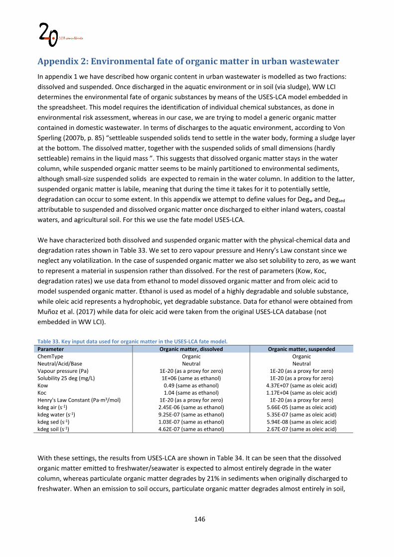
146

Appendix 2: Environmental fate of organic matter in urban wastewater

In appendix 1 we have described how organic content in urban wastewater is modelled as two fractions: dissolved and suspended. Once discharged in the aquatic environment or in soil (via sludge), WW LCI determines the environmental fate of organic substances by means of the USES-LCA model embedded in the spreadsheet. This model requires the identification of individual chemical substances, as done in environmental risk assessment, whereas in our case, we are trying to model a generic organic matter contained in domestic wastewater. In terms of discharges to the aquatic environment, according to Von Sperling (2007b, p. 85) “settleable suspended solids tend to settle in the water body, forming a sludge layer at the bottom. The dissolved matter, together with the suspended solids of small dimensions (hardly settleable) remains in the liquid mass ”. This suggests that dissolved organic matter stays in the water column, while suspended organic matter seems to be mainly partitioned to environmental sediments, although small-size suspended solids are expected to remain in the water column. In addition to the latter, suspended organic matter is labile, meaning that during the time it takes for it to potentially settle, degradation can occur to some extent. In this appendix we attempt to define values for Degw and Degsed attributable to suspended and dissolved organic matter once discharged to either inland waters, coastal waters, and agricultural soil. For this we use the fate model USES-LCA. We have characterized both dissolved and suspended organic matter with the physical-chemical data and degradation rates shown in Table 33. We set to zero vapour pressure and Henry’s Law constant since we neglect any volatilization. In the case of suspended organic matter we also set solubility to zero, as we want to represent a material in suspension rather than dissolved. For the rest of parameters (Kow, Koc, degradation rates) we use data from ethanol to model dissoved organic matter and from oleic acid to model suspended organic matter. Ethanol is used as model of a highly degradable and soluble substance, while oleic acid represents a hydrophobic, yet degradable substance. Data for ethanol were obtained from Muñoz et al. (2017) while data for oleic acid were taken from the original USES-LCA database (not embedded in WW LCI). Table 33. Key input data used for organic matter in the USES-LCA fate model. Parameter Organic matter, dissolved Organic matter, suspended ChemType Organic Organic Neutral/Acid/Base Neutral Neutral Vapour pressure (Pa) 1E-20 (as a proxy for zero) 1E-20 (as a proxy for zero) Solubility 25 deg (mg/L) 1E+06 (same as ethanol) 1E-20 (as a proxy for zero) Kow 0.49 (same as ethanol) 4.37E+07 (same as oleic acid) Koc 1.04 (same as ethanol) 1.17E+04 (same as oleic acid) Henry's Law Constant (Pa·m3/mol) 1E-20 (as a proxy for zero) 1E-20 (as a proxy for zero) kdeg air (s-1) 2.45E-06 (same as ethanol) 5.66E-05 (same as oleic acid) kdeg water (s-1) 9.25E-07 (same as ethanol) 5.35E-07 (same as oleic acid) kdeg sed (s-1) 1.03E-07 (same as ethanol) 5.94E-08 (same as oleic acid) kdeg soil (s-1) 4.62E-07 (same as ethanol) 2.67E-07 (same as oleic acid) With these settings, the results from USES-LCA are shown in Table 34. It can be seen that the dissolved organic matter emitted to freshwater/seawater is expected to almost entirely degrade in the water column, whereas particulate organic matter degrades by 21% in sediments when originally discharged to freshwater. When an emission to soil occurs, particulate organic matter degrades almost entirely in soil,

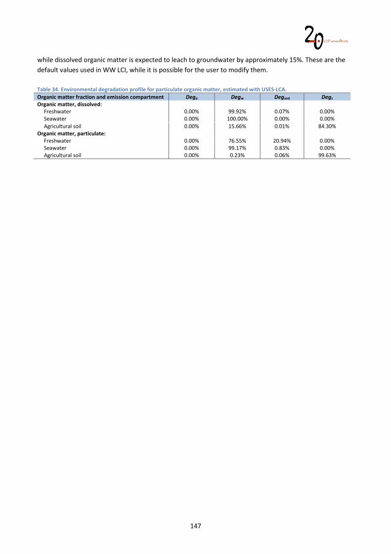
147

while dissolved organic matter is expected to leach to groundwater by approximately 15%. These are the default values used in WW LCI, while it is possible for the user to modify them. Table 34. Environmental degradation profile for particulate organic matter, estimated with USES-LCA. Organic matter fraction and emission compartment Dega Degw Degsed Degs Organic matter, dissolved: Freshwater 0.00% 99.92% 0.07% 0.00% Seawater 0.00% 100.00% 0.00% 0.00% Agricultural soil 0.00% 15.66% 0.01% 84.30% Organic matter, particulate: Freshwater 0.00% 76.55% 20.94% 0.00% Seawater 0.00% 99.17% 0.83% 0.00% Agricultural soil 0.00% 0.23% 0.06% 99.63%

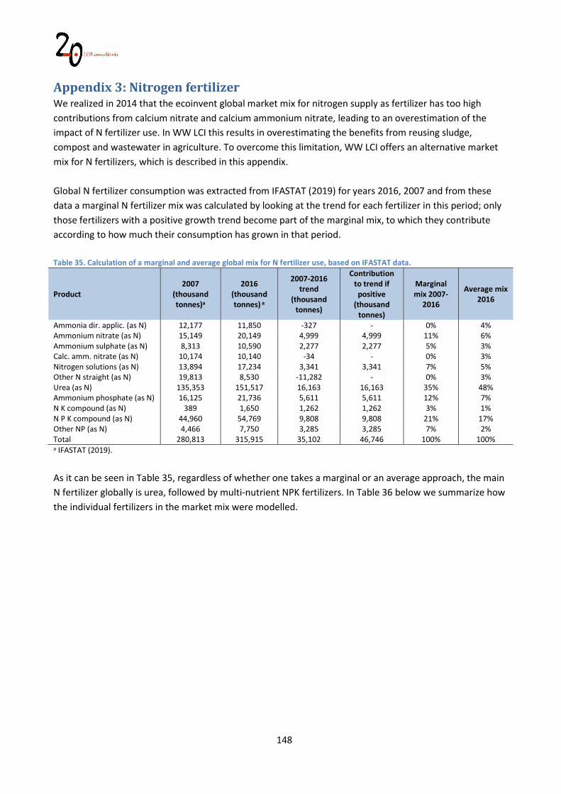
148

Appendix 3: Nitrogen fertilizer We realized in 2014 that the ecoinvent global market mix for nitrogen supply as fertilizer has too high contributions from calcium nitrate and calcium ammonium nitrate, leading to an overestimation of the impact of N fertilizer use. In WW LCI this results in overestimating the benefits from reusing sludge, compost and wastewater in agriculture. To overcome this limitation, WW LCI offers an alternative market mix for N fertilizers, which is described in this appendix. Global N fertilizer consumption was extracted from IFASTAT (2019) for years 2016, 2007 and from these data a marginal N fertilizer mix was calculated by looking at the trend for each fertilizer in this period; only those fertilizers with a positive growth trend become part of the marginal mix, to which they contribute according to how much their consumption has grown in that period. Table 35. Calculation of a marginal and average global mix for N fertilizer use, based on IFASTAT data.

Product 2007

(thousand tonnes)a

2016 (thousand tonnes) a

2007-2016 trend

(thousand tonnes)

Contribution to trend if positive

(thousand tonnes)

Marginal mix 2007-

2016

Average mix 2016

Ammonia dir. applic. (as N) 12,177 11,850 -327 - 0% 4% Ammonium nitrate (as N) 15,149 20,149 4,999 4,999 11% 6% Ammonium sulphate (as N) 8,313 10,590 2,277 2,277 5% 3% Calc. amm. nitrate (as N) 10,174 10,140 -34 - 0% 3% Nitrogen solutions (as N) 13,894 17,234 3,341 3,341 7% 5% Other N straight (as N) 19,813 8,530 -11,282 - 0% 3% Urea (as N) 135,353 151,517 16,163 16,163 35% 48% Ammonium phosphate (as N) 16,125 21,736 5,611 5,611 12% 7% N K compound (as N) 389 1,650 1,262 1,262 3% 1% N P K compound (as N) 44,960 54,769 9,808 9,808 21% 17% Other NP (as N) 4,466 7,750 3,285 3,285 7% 2% Total 280,813 315,915 35,102 46,746 100% 100% a IFASTAT (2019).

As it can be seen in Table 35, regardless of whether one takes a marginal or an average approach, the main N fertilizer globally is urea, followed by multi-nutrient NPK fertilizers. In Table 36 below we summarize how the individual fertilizers in the market mix were modelled.

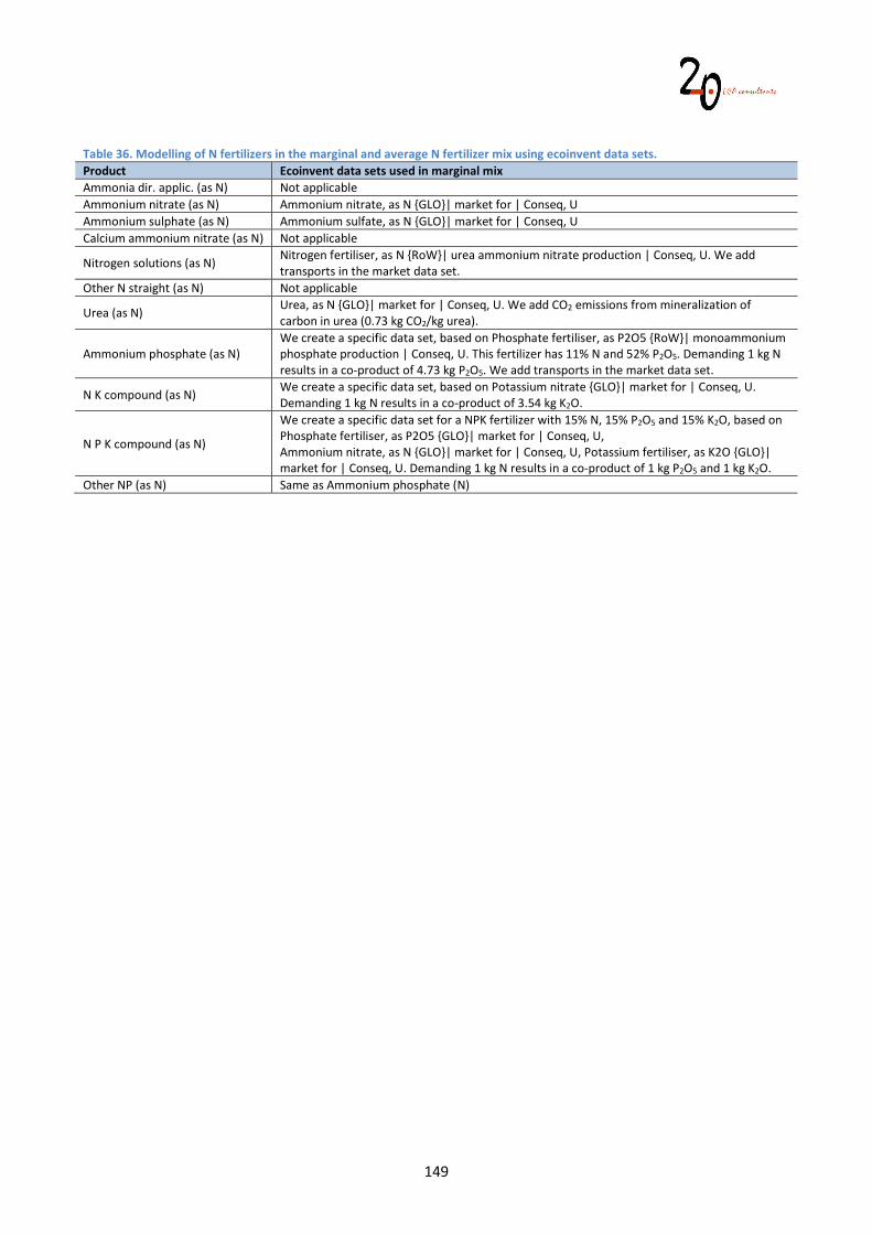
149

Table 36. Modelling of N fertilizers in the marginal and average N fertilizer mix using ecoinvent data sets. Product Ecoinvent data sets used in marginal mix Ammonia dir. applic. (as N) Not applicable Ammonium nitrate (as N) Ammonium nitrate, as N {GLO}| market for | Conseq, U Ammonium sulphate (as N) Ammonium sulfate, as N {GLO}| market for | Conseq, U Calcium ammonium nitrate (as N) Not applicable

Nitrogen solutions (as N) Nitrogen fertiliser, as N {RoW}| urea ammonium nitrate production | Conseq, U. We add transports in the market data set.

Other N straight (as N) Not applicable

Urea (as N) Urea, as N {GLO}| market for | Conseq, U. We add CO2 emissions from mineralization of carbon in urea (0.73 kg CO2/kg urea).

Ammonium phosphate (as N) We create a specific data set, based on Phosphate fertiliser, as P2O5 {RoW}| monoammonium phosphate production | Conseq, U. This fertilizer has 11% N and 52% P2O5. Demanding 1 kg N results in a co-product of 4.73 kg P2O5. We add transports in the market data set.

N K compound (as N) We create a specific data set, based on Potassium nitrate {GLO}| market for | Conseq, U. Demanding 1 kg N results in a co-product of 3.54 kg K2O.

N P K compound (as N)

We create a specific data set for a NPK fertilizer with 15% N, 15% P2O5 and 15% K2O, based on Phosphate fertiliser, as P2O5 {GLO}| market for | Conseq, U, Ammonium nitrate, as N {GLO}| market for | Conseq, U, Potassium fertiliser, as K2O {GLO}| market for | Conseq, U. Demanding 1 kg N results in a co-product of 1 kg P2O5 and 1 kg K2O.

Other NP (as N) Same as Ammonium phosphate (N)