WARP: On-the-fly Program Synthesis for Agile, Real-time, and Reliable Wireless Networks Ryan Brummet, Md Kowsar Hossain, Octav Chipara, Ted Herman, and Steve Goddard (ryan-brummet,mdkowsar-hossain,octav-chipara,ted-herman,steve-goddard)@uiowa.edu Department of Computer Science, University of Iowa Iowa City, USA ABSTRACT Emerging Industrial Internet-of-Things systems require wireless so- lutions to connect sensors, actuators, and controllers as part of high data rate feedback-control loops over real-time flows. A key chal- lenge is to provide predictable performance and agility in response to fluctuations in link quality, variable workloads, and topology changes. We propose WARP to address this challenge. WARP uses programs to specify a network’s behavior and includes a synthesis procedure to automatically generate such programs from a high- level specification of the system’s workload and topology. WARP has three unique features: (1) WARP uses a domain-specific language to specify stateful programs that include conditional statements to control when a flow’s packets are transmitted. The execution paths of programs depend on the pattern of packet losses observed at run- time, thereby enabling WARP to readily adapt to packet losses due to short-term variations in link quality. (2) Our synthesis technique uses heuristics to improve network performance by considering multiple packet loss patterns and associated execution paths when determining the transmissions performed by nodes. Furthermore, the generated programs ensure that the likelihood of a flow deliver- ing its packets by its deadline exceeds a user-specified threshold. (3) WARP can adapt to workload and topology changes without explicitly reconstructing a network’s program based on the observation that nodes can independently synthesize the same program when they share the same workload and topology information. Simulations show that WARP improves network throughput for data collection, dissemination, and mixed workloads on two realistic topologies. Testbed experiments show that WARP reduces the time to add new flows by 5 times over a state-of-the-art centralized control plane and guarantees the real-time and reliability of all flows. CCS CONCEPTS • Networks → Network dynamics; Network reliability; Cyber- physical networks. KEYWORDS Wireless networks, real-time wireless networks, reliability, software synthesis ACM Reference Format: Ryan Brummet, Md Kowsar Hossain, Octav Chipara, Ted Herman, and Steve Goddard. 2021. WARP: On-the-fly Program Synthesis for Agile, Real-time, and Reliable Wireless Networks. In The 20th International Conference on Information Processing in Sensor Networks (co-located with CPS-IoT Week IPSN ’21, May 18–21, 2021, Nashville, TN, USA 2021. ACM ISBN 978-1-4503-8098-0/21/05. https://doi.org/10.1145/3412382.3458270 2021) (IPSN ’21), May 18–21, 2021, Nashville, TN, USA. ACM, New York, NY, USA, 14 pages. https://doi.org/10.1145/3412382.3458270 1 INTRODUCTION Over the last decade, we have seen the development of transmission scheduling techniques (see [18, 21] for overviews) and their wide- spread adoption in process control industries (e.g., [18, 22]). These efforts have primarily focused on supporting real-time and reliable communication over low-power networks composed of resource- constrained devices that often run on batteries. In contrast, the future Industrial Internet-of-Things (IIoT) applications will employ sophisticated sensors such as cameras, microphones, or LIDAR, which generate large volumes of data. The generated data will be processed by embedded devices that are (grid) powered and have sufficient processing resources to run machine learning and computer vision algorithms. Such IIoT applications require that, in addition to real-time and reliable communication, wireless protocols also support higher data rates, handle variable workloads, and cope with short-term fluctuations in link quality and topology changes. As a concrete example, consider a John Deere’s 32-row planter with 15 sensors per row [7], each of the 480 sensors generating 5 samples per second. A modern John Deere herbicide sprayer requires even higher throughput to handle the traffic generated by the approximately 250 cameras necessary for “sub-inch accu- racy of the application of herbicide” [13]. Each sensor is powered with a serial line running along the tractor’s boom or chassis and wirelessly transmits images over multi-hop real-time flows to the tractor processing platform where machine learning techniques are used to classify the types of weeds in the video stream. In re- sponse, commands are sent to herbicide spray nozzles to target the identified weeds. Mesh networking techniques can be applied for fault-tolerance. An effective wireless solution must also handle the dynamic wireless conditions observed in the field (e.g., variable humidity and dust, which affects signal propagation) and adapt communication schedules as the sensing rates change with the driving speed and field conditions. The contribution of this paper is WARP – a novel approach that uses software synthesis to meet the demands of the future IIoT ap- plications. Software synthesis usually relies on SMT solvers and re- quires resource-rich machines. These techniques need to be adapted to embedded devices and extended to build wireless networks that provide real-time and reliable performance in the presence of net- work dynamics. Three components support this goal: (1) a data plane whose operation is specified as programs that are more ex- pressive than traditional schedules; (2) a scalable software synthesis procedure that generates programs that satisfy the flows’ deadline

Welcome message from author
This document is posted to help you gain knowledge. Please leave a comment to let me know what you think about it! Share it to your friends and learn new things together.
Transcript
WARP: On-the-fly Program Synthesis for Agile, Real-time, andReliable Wireless Networks
Ryan Brummet, Md Kowsar Hossain, Octav Chipara, Ted Herman, and Steve Goddard
(ryan-brummet,mdkowsar-hossain,octav-chipara,ted-herman,steve-goddard)@uiowa.edu
Department of Computer Science, University of Iowa
Iowa City, USA
ABSTRACTEmerging Industrial Internet-of-Things systems require wireless so-
lutions to connect sensors, actuators, and controllers as part of high
data rate feedback-control loops over real-time flows. A key chal-
lenge is to provide predictable performance and agility in response
to fluctuations in link quality, variable workloads, and topology
changes. We propose WARP to address this challenge. WARP uses
programs to specify a network’s behavior and includes a synthesis
procedure to automatically generate such programs from a high-
level specification of the system’s workload and topology. WARP hasthree unique features: (1) WARP uses a domain-specific language to
specify stateful programs that include conditional statements to
control when a flow’s packets are transmitted. The execution paths
of programs depend on the pattern of packet losses observed at run-
time, thereby enabling WARP to readily adapt to packet losses due
to short-term variations in link quality. (2) Our synthesis technique
uses heuristics to improve network performance by considering
multiple packet loss patterns and associated execution paths when
determining the transmissions performed by nodes. Furthermore,
the generated programs ensure that the likelihood of a flow deliver-
ing its packets by its deadline exceeds a user-specified threshold. (3)
WARP can adapt toworkload and topology changeswithout explicitlyreconstructing a network’s program based on the observation that
nodes can independently synthesize the same program when they
share the same workload and topology information. Simulations
show that WARP improves network throughput for data collection,
dissemination, and mixed workloads on two realistic topologies.
Testbed experiments show that WARP reduces the time to add new
flows by 5 times over a state-of-the-art centralized control plane
and guarantees the real-time and reliability of all flows.
CCS CONCEPTS•Networks→Networkdynamics;Network reliability;Cyber-physical networks.
KEYWORDSWireless networks, real-time wireless networks, reliability, software
synthesis
ACM Reference Format:Ryan Brummet, Md Kowsar Hossain, Octav Chipara, Ted Herman, and Steve
Goddard. 2021. WARP: On-the-fly Program Synthesis for Agile, Real-time,
and Reliable Wireless Networks. In The 20th International Conference onInformation Processing in Sensor Networks (co-located with CPS-IoT Week
IPSN ’21, May 18–21, 2021, Nashville, TN, USA2021. ACM ISBN 978-1-4503-8098-0/21/05.
https://doi.org/10.1145/3412382.3458270
2021) (IPSN ’21), May 18–21, 2021, Nashville, TN, USA. ACM, New York, NY,
USA, 14 pages. https://doi.org/10.1145/3412382.3458270
1 INTRODUCTIONOver the last decade, we have seen the development of transmission
scheduling techniques (see [18, 21] for overviews) and their wide-
spread adoption in process control industries (e.g., [18, 22]). These
efforts have primarily focused on supporting real-time and reliable
communication over low-power networks composed of resource-
constrained devices that often run on batteries. In contrast, the
future Industrial Internet-of-Things (IIoT) applications will employ
sophisticated sensors such as cameras, microphones, or LIDAR,
which generate large volumes of data. The generated data will
be processed by embedded devices that are (grid) powered and
have sufficient processing resources to run machine learning and
computer vision algorithms. Such IIoT applications require that, in
addition to real-time and reliable communication, wireless protocols
also support higher data rates, handle variable workloads, and cope
with short-term fluctuations in link quality and topology changes.
As a concrete example, consider a John Deere’s 32-row planter
with 15 sensors per row [7], each of the 480 sensors generating
5 samples per second. A modern John Deere herbicide sprayer
requires even higher throughput to handle the traffic generated
by the approximately 250 cameras necessary for “sub-inch accu-
racy of the application of herbicide” [13]. Each sensor is powered
with a serial line running along the tractor’s boom or chassis and
wirelessly transmits images over multi-hop real-time flows to thetractor processing platform where machine learning techniques
are used to classify the types of weeds in the video stream. In re-
sponse, commands are sent to herbicide spray nozzles to target the
identified weeds. Mesh networking techniques can be applied for
fault-tolerance. An effective wireless solution must also handle the
dynamic wireless conditions observed in the field (e.g., variable
humidity and dust, which affects signal propagation) and adapt
communication schedules as the sensing rates change with the
driving speed and field conditions.
The contribution of this paper is WARP – a novel approach that
uses software synthesis to meet the demands of the future IIoT ap-
plications. Software synthesis usually relies on SMT solvers and re-
quires resource-rich machines. These techniques need to be adapted
to embedded devices and extended to build wireless networks that
provide real-time and reliable performance in the presence of net-
work dynamics. Three components support this goal: (1) a data
plane whose operation is specified as programs that are more ex-
pressive than traditional schedules; (2) a scalable software synthesis
procedure that generates programs that satisfy the flows’ deadline
IPSN ’21, May 18–21, 2021, Nashville, TN, USA Ryan Brummet, Md Kowsar Hossain, Octav Chipara, Ted Herman, and Steve Goddard
and reliability constraints; and (3) an efficient control plane to han-
dle workload and topology changes.
A network operator programs a WARP network by specifying
its workload. The workload is composed of real-time flows that
carry data between sensors, controllers, and actuators. Flows are
periodic, may span multiple hops, and deliver packets subject to
deadline and reliability constraints. We have developed techniques
to synthesize programs that specify the data plane’s behavior based
on the supplied workload and topology. The programs are written
in a domain-specific language (DSL) that can express more com-
plex behaviors than traditional scheduling approaches. A feature
that distinguishes programs from schedules is that programs are
stateful and may include conditional statements. The execution
of an instruction to forward a flow’s packet changes the flow’s
state to indicate whether the transmission succeeded or not. Sub-
sequent instructions may query this state and make conditional
decisions on what packets to forward. The combination of state
and conditional actions leads to programs havingmultiple executionpaths that depend on the pattern of packet losses observed during
their execution. This opens the opportunity to synthesize programs
whose actions are optimized to handle likely packet loss patterns
and readily adapt to the rapidly evolving packet loss patterns ob-
served during their execution. Our experiments demonstrate that
programs provide higher performance than scheduling approaches
while remaining simple to analyze.
The synthesis procedure ensures that the execution of programs
will not result in nodes performing conflicting operations. Addition-
ally, the synthesis procedure also guarantees that the likelihood of a
flow’s packets reaching their destination by their deadline exceeds
a user-specified threshold. This property holds under our Threshold
Reliability Model (TLR) that allows link quality to vary arbitrarily
from slot-to-slot but always remains above a minimum level of relia-
bility. WARP cannot guarantee the network’s performance when the
quality of links falls below the minimum packet delivery rate (PDR).
In this case, the minimum PDR may be lowered or the flow’s routes
may need to be adjusted to include links that meet the minimum
PDR. TLR is inspired by Emerson’s best practices for deploying
WirelessHART networks [19], which encourage network operators
to ensure that links have a minimum PDR of 60% – 70% at deploy-
ment time. We have developed a computationally efficient approach
to reason about the probability of delivering packets under TLR by
considering all packet loss scenarios and their associated execution
paths and likelihoods.
WARP includes a decentralized control plane that can adapt to
workload and topology changes without synthesizing new pro-
grams. Our insight is that when nodes share the same topology and
workload information, they can run the same synthesis procedure
locally to generate identical programs. This approach significantly
improves the network’s agility since workload or topology changes
only require disseminating the added or modified flows and routes.
Such updates can be encoded efficiently, most often, in a single
packet. However, the challenge is to implement WARP’s programsynthesis on embedded devices on which it is infeasible to run
SMT solvers that are commonly used in software synthesis. Within
10 ms slots, WARP can synthesize and execute programs on-the-fly
on TelosB and Decawave DWM1001 devices.
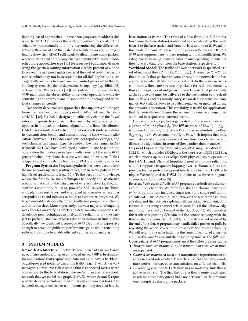
Protocol Data Rate Workload EnergyWirelessHART low fixed constrained
REACT [15] low variable constrained
FD-PaS [24]
DistributedHART [20]
WARP high variable unconstrained
Table 1: Requirements space of IIoT protocols
We have evaluated WARP through simulations and testbed exper-
iments using workloads typical in IIoT systems. Our simulations
indicate that WARP can significantly improve throughput across
typically IIoT workloads in two realistic topologies. We have im-
plemented our techniques on Decawave DWM1001, which use
802.15.4a radios, and on TelosB, which use 802.15.4 radios. The
testbed experiments demonstrate the feasibility of using synthe-
sis techniques to construct programs on-the-fly. Furthermore, our
experiments validate that WARP can satisfy the real-time and relia-
bility constraints of flows and adapt quickly to workload changes.
2 RELATEDWORKData plane: At the heart of wireless networks that support real-time communication are transmission scheduling techniques (e.g.,
[16, 20, 23, 24] and surveys [18, 21]). For example, WirelessHART
specifies the data plane’s behavior using a (repeating) super-frame,
a two-dimension matrix whose cells grant access to a specific slot
and channel. Real-time traffic is supported by using dedicated cells
in which a single transmission is scheduled, while best-effort traffic
is supported using shared slots. Under these and similar assump-
tions about the data plane, researchers have developed numerous
algorithms to construct efficient schedules under different workload
scenarios and analyze their real-time and reliability performance.
A contribution of WARP is an intermediary language to specify a
“smart” data plane that allows a richer set of behaviors, including
the ability of multiple real-time flows to share the same entry for
improved performance.
The closest related work is Recorp [4], which proposes a policy-
based approach that, similar to WARP, can also share entries across
multiple flows. WARP improves upon Recorp in several important
ways: First, WARP’s DSL can specify more expressive programs than
Recorp policies. As a consequence, WARP can provide better perfor-
mance under more varied workloads than Recorp. Second, Recorpis only suitable for IIoT applications whose workloads are fixed and
known apriori since it may take up to aminute to construct a Recorp
policy. In contrast, WARP can synthesize and execute programs on-
the-fly within 10 ms slots on embedded platforms. Finally, WARPincludes a new decentralized control plan that can adapt effectively
to changes in topology and workload.
Control plane: A common critique of approaches like Wire-
lessHART is that their centralized design leads to networks that
cannot adapt effectively to dynamics. Indeed, this is problematic
since any workload or topology changes requires creating a new
super-frame and disseminating it to all nodes. This process can be
particularly expensive when the super-frame is large and does not
fit within a single packet. Four broad approaches — incremental
scheduling, autonomous scheduling, distributed scheduling, and
WARP: On-the-fly Program Synthesis for Agile, Real-time, and Reliable Wireless Networks IPSN ’21, May 18–21, 2021, Nashville, TN, USA
flooding-based approaches — have been proposed to address this
issue. REACT [15] reduces the control overhead by constructing
schedules incrementally and only disseminating the differences
between the current and the updated schedule. However, our exper-
iments show that REACT still needs to disseminate many packets
when the workload or topology changes significantly. Autonomous
scheduling approaches (see [11] for a survey) build super-frames
using the (partial) routing information already present at a node.
However, the increased agility comes at the cost of real-time perfor-
mance, which may not be acceptable for all IIoT applications. An
elegant alternative is to avoid complex control planes altogether by
building systems that do not depend on the topology (e.g., Blink [25]
or Low-power Wireless Bus [12]). In contrast to these approaches,
WARP maintains the observability of network operations while de-
centralizing the control plane to support both topology and work-
load changes efficiently.
Two recent decentralized approaches that support real-time per-
formance have been recently proposed: FD-PaS [24] and Distribut-
edHART [20]. FD-PaS is designed to efficiently change the flows’
rates in response to external disturbances by piggybacking rate
updates in the packet acknowledgments of a flow. Distributed-
HART uses a node-level scheduling where each node schedules
its transmissions locally and online through a time window allo-
cation. However, FD-PaS does not consider topology changes, and
such changes can trigger expensive network-wide changes in Dis-
tributedHART. We have developed a control plane based on the
observation that nodes can independently construct the same WARPprogram when they share the same workload information. Table 1
compares and contrasts the features of WARP and related protocols.
Program Synthesis: Program synthesis has been used to syn-
thesize network updates, routing tables, and network policies from
high-level specifications (e.g., [10]). To the best of our knowledge,
we are the first to use such techniques to specify and synthesize
programs that control the data plane of wireless networks. Program
synthesis commonly relies on powerful SMT solvers, machines
with plentiful resources, and is applied in scenarios where it is
acceptable to spend minutes to hours to synthesize programs. We
target embedded devices that must synthesize programs on-the-fly
within 10 ms slots. More importantly, the vast majority of ongoing
work focuses on verifying safety and deterministic properties. We
developed new techniques to analyze the reliability of flows sub-
ject to probabilistic packet losses due to variations in link quality.
Specifically, we identified a subset of WARP DSL that is expressive
enough to provide significant performance gains while remaining
sufficiently simple to enable efficient synthesis and analysis.
3 SYSTEM MODELSNetworkArchitecture:A network is comprised of a network man-ager, a base station, and up to a hundred nodes. WARP is best-suited
for applications that require high data rates and have a backbone
of grid-powered nodes to carry this traffic (e.g., [2, 6]). A networkmanager is a resource-rich machine that is connected over a wired
connection to the base station. The nodes form a wireless mesh
network that we model as a graph 𝐺 (N , E), where N and E repre-
sent the devices (including the base station) and wireless links. The
network manager constructs a minimum spanning tree that has the
base station as its root. The route of a flow from 𝐴 to 𝐵 (both dis-
tinct from the base station) is obtained by concatenating the route
from 𝐴 to the base station and from the base station to 𝐵. We adopt
this model for consistency with prior work on WirelessHART, but
WARP also supports peer-to-peer routing without modification. We
categorize flows as upstream or downstream depending on whether
they forward data to or from the base station, respectively.
Workload Model: The traffic of a WARP network is specified as a
set of real-time flows F = {𝐹0, 𝐹1, . . . , 𝐹𝑁 }. A real-time flow 𝐹𝑖 is a
fixed route Γ𝑖 that packets traverse through the network and has
several associated attributes described next. In the wider network
community, flows are streams of packets; for real-time contexts,
flows are sequences of independent packets generated periodically
at the source and must be delivered to the destination by the dead-
line. A flow’s packets usually carry sensor data or actuation com-
mands. WARP allows flows to be added, removed, or modified during
the network’s operation. This capability is useful for applications
that dynamically reconfigure the sensors they use or change their
workload in response to external events.
For each flow 𝐹𝑖 , a packet is generated on the source node with
a period of 𝑃𝑖 and phase 𝜙𝑖 . The k𝑡ℎ
instance of flow 𝐹𝑖 — 𝐽𝑖,𝑘 —
is released at time 𝑟𝑖,𝑘 = 𝜙𝑖 + 𝑘 ∗ 𝑃𝑖 and has an absolute deadline
𝑑𝑖,𝑘 = 𝑟𝑖,𝑘 + 𝐷𝑖 . We assume that 𝐷𝑖 ≤ 𝑃𝑖 , which implies that only
one instance of a flow is released at any time. For clarity, we will
discuss the algorithms in terms of flows rather than instances.
Physical Layer: At the physical layer, WARP may use either IEEE
802.15.4, which provides 250 kbps, or themore recent IEEE 802.15.4a,
which supports up to 27.24 Mbps. Both physical layers operate in
the 2.4 GHz band. Channel hopping is used to improve reliability.
802.15.4 supports frequency hopping over 16 channels. 802.15.4a
provides further protection against interference by using UWB tech-
niques. We configured the DWM1001 radios to use three orthogonal
channels, as described in [8].
Entries, Pushes, and Pulls: WARP programs use both time division
and multiple channels. We refer to a slot and channel pair as anentry. Programs may include a single push or a single pull withinan entry of 10 ms. A push(𝐹𝑖 , #ch) involves the sender transmitting
𝐹𝑖 ’s data and the receiver replying with an acknowledgment, both
transmissions using channel #ch. A push fails if the acknowledg-
ment is not received by the end of the slot. A pull(𝐹𝑖 , #ch) involvesthe receiver requesting 𝐹𝑖 ’s data and the sender replying with the
flow’s data on channel #ch. A pull fails if the data is not received bythe end of the slot. A program may handle failed pushes or pulls byrepeating the action several times to achieve the desired reliability.
We will refer to the node initiating the communication of a push or
a pull as the coordinator and the responding node as the follower.Constraints:A WARP programmust meet the following constraints:
• Transmission constraints: A node transmits or receives at most
once per slot.
• Channel constraints: At most one transmission is performed in an
entry to avoid intra-network interference. Additionally, a node
must perform consecutive transmissions on different channels.
• Forwarding constraints: Each flow has at most one link that is
active in any slot. The first link on the flow’s route is activated
at release time; subsequent links are activated as the previous
ones complete relaying the packets.
IPSN ’21, May 18–21, 2021, Nashville, TN, USA Ryan Brummet, Md Kowsar Hossain, Octav Chipara, Ted Herman, and Steve Goddard
• Real-time and reliability constraint: The likelihood that the pack-
ets of a flow reach their destination before their deadline exceeds
an end-to-end probability target.
4 WARPLayer Responsibilities: WARP is a practical and effective solution
for IIoT applications that require high-data rates, real-time, and
reliable communication in dynamic wireless environments. The
data plane handles packet losses due to probabilistic and variable
links, whereas the control plane handles topology and workload
changes. A central aspect of WARP is that each node executes a state-
ful program that controls when it transmits the packets of real-time
flows. Programs specified using the DSL described in Section 4.1
can express more intricate actions than possible using traditional
schedules. A node’s program tracks the success or failure of a flows’
transmissions and, based on this state, it executes different trans-
missions depending on the pattern of observed packet losses. This
approach improves network performance significantly. In Section
4.2, we propose techniques to analyze a program’s execution in the
presence of packet losses and introduce the TLR model to specify
how the quality of links vary.
Data Plane: WARP incorporates a scalable program synthesis pro-
cedure that turns a high-level specification of the workload and
topology into a program that is executed by the network. The
synthesis procedure incorporates a generator and an estimatordescribed in Section 4.3.1 and 4.3.2, respectively. The estimatorreasons about the possible execution paths of a program under
all failure scenarios and determines the likelihood of each reach-
able state (under the assumptions of the TLR model). Based on
this information, the generator heuristically increases the number
of flows that execute in each slot across multiple possible failure
scenarios. The synthesized programs’ execution guarantees that
the likelihood of each flow’s packets reaching their destination
by its deadline exceeds a user-specified threshold. This guarantee
holds only when the network’s behavior is consistent with the TLR
model: (1) consecutive transmissions are independent and (2) the
chance of successful transmission can vary, but it always exceeds a
minimum threshold𝑚. When the network deviates from the TLR
model, either new routes that use links that conform to the TLR
model should be selected or the value of𝑚 should be lowered. The
synthesis procedure may fail to generate a program when the work-
load is close to the network’s capacity. In this case, the workload has
to be adjusted manually by the network operator or automatically
using rate control mechanisms. As discussed next, our goal is to
run the synthesis on embedded devices. Therefore, we focus on
synthesis techniques that use light-weight heuristics.
Control Plane: Similar toWirelessHART, WARPmanages the topol-
ogy and workload information centrally. However, we decentralize
the synthesis and adaption to workload changes, as detailed in
Section 4.4. In contrast to scheduling approaches, WARP does not
construct an explicit schedule but instead runs the synthesis proce-
dure on each node on-the-fly to determine its actions in a slot. All
the nodes will construct the same program as long as they share
the same workload and topology information. The decentralized
control plane handles workload and topology changes by dissemi-
nating only the updated workload or topology information. This
fragment := release-blk; action_blk; drop_blkrelease_blk := release(flow, link); | release_blkdrop_blk := drop(flow); | drop_blkaction_blk := action | if-statementif-statement := if bool-expr then action else-partelse-part := else action_blk | 𝜖bool-expr := has(flow) | !has(flow)action := pull(flow, channel) | push(flow, channel) |
wait(channel) | sleep
Figure 1: EBNF rules of a WARP fragment
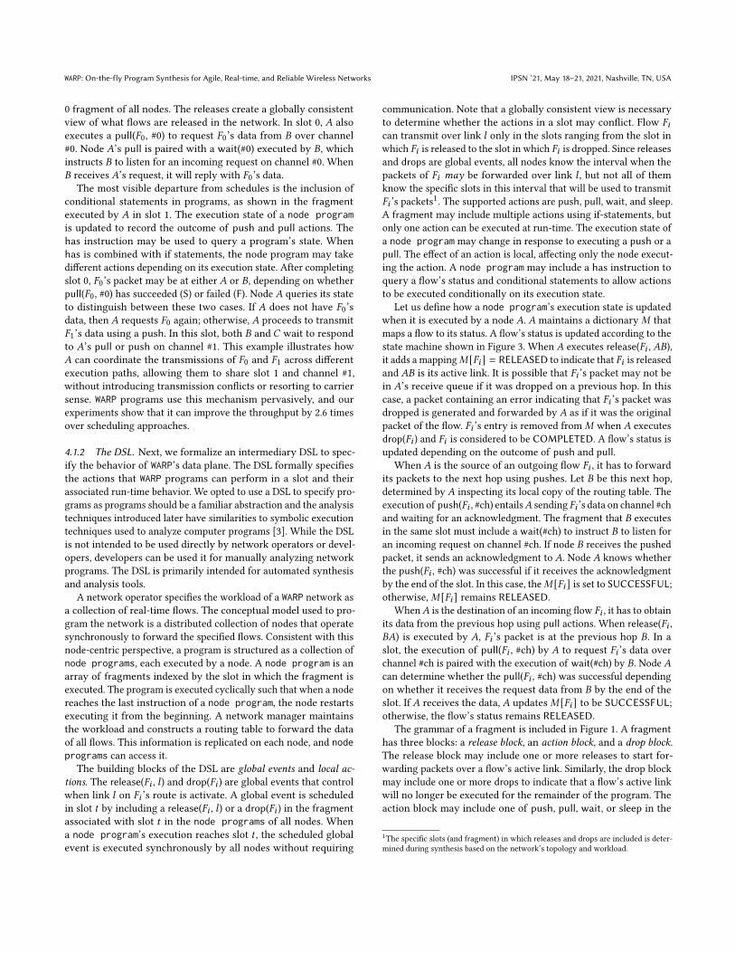
B
A
C
F0 F1
(a) Topology
Slot Node A Node B Node C
0 release(𝐹0 , 𝐵𝐴) release(𝐹0 , 𝐵𝐴) release(𝐹0 , 𝐵𝐴)release(𝐹1 ,𝐴𝐶) release(𝐹1 ,𝐴𝐶) release(𝐹1 ,𝐴𝐶)pull(𝐹0 , #0) wait(#0)
1 if !has(𝐹0) then pull(𝐹0 , #1) wait(#1) wait(#1)else push(𝐹1 , #1)
2 push(𝐹1 , #2) sleep wait(#2)
(b) WARP program
F0: FF1: F
10%
F0: FF1: F
100%
F0: SF1: F
90%
F0: FF1: F
1%
F0: SF1: F
18%
F0: SF1: S
81%
F0: FF1: F
0.1%
F0: SF1: F
2.7%
F0: SF1: S
97.2%
pull(F0,#1)
pull(F0,#0)
pull(F0,#0) pull(F0,#1)
pull(F1,#1)
pull(F1,#1)
pull(F1,#2)
pull(F1,#2)
pull(F1,#2)
pull(F1,#2)
(c) Node 𝐴’s execution DAG
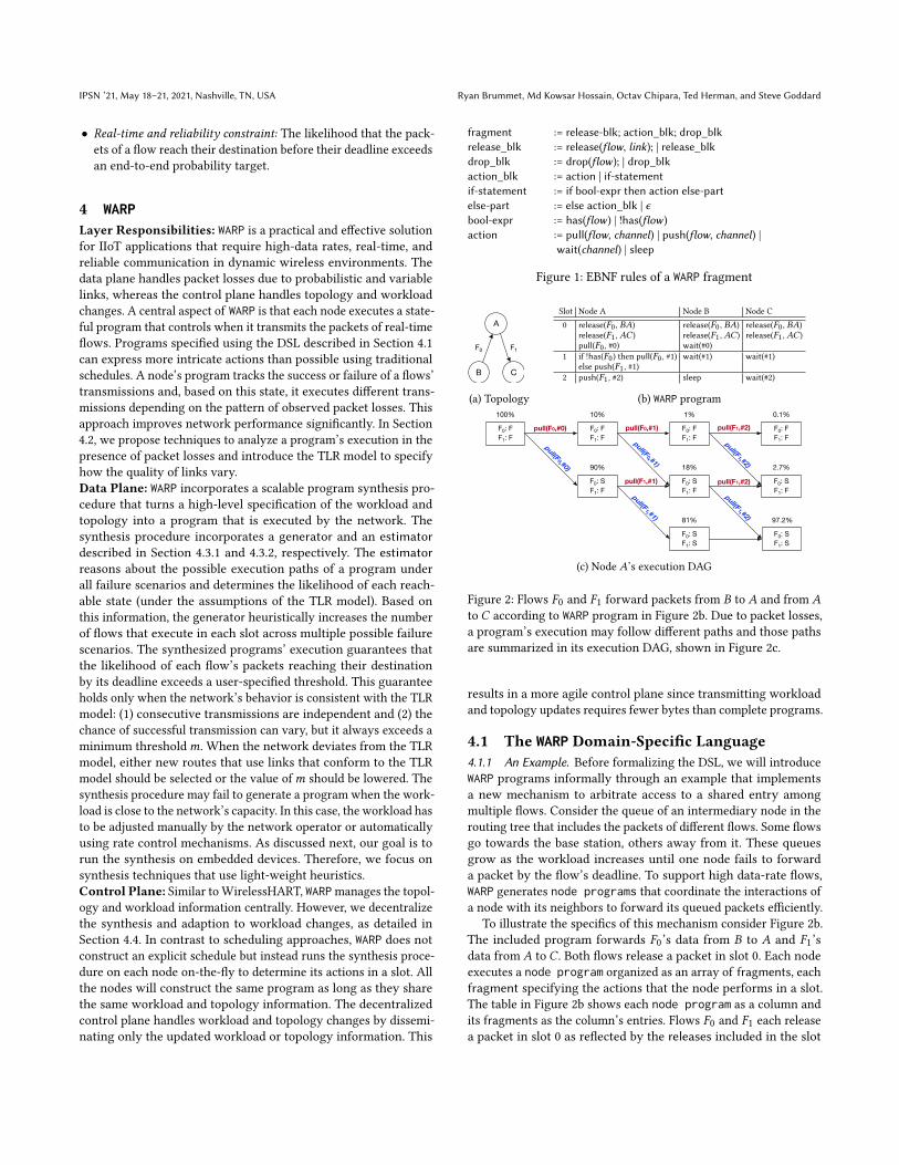
Figure 2: Flows 𝐹0 and 𝐹1 forward packets from 𝐵 to 𝐴 and from 𝐴
to 𝐶 according to WARP program in Figure 2b. Due to packet losses,
a program’s execution may follow different paths and those paths
are summarized in its execution DAG, shown in Figure 2c.
results in a more agile control plane since transmitting workload
and topology updates requires fewer bytes than complete programs.
4.1 The WARP Domain-Specific Language4.1.1 An Example. Before formalizing the DSL, we will introduce
WARP programs informally through an example that implements
a new mechanism to arbitrate access to a shared entry among
multiple flows. Consider the queue of an intermediary node in the
routing tree that includes the packets of different flows. Some flows
go towards the base station, others away from it. These queues
grow as the workload increases until one node fails to forward
a packet by the flow’s deadline. To support high data-rate flows,
WARP generates node programs that coordinate the interactions of
a node with its neighbors to forward its queued packets efficiently.
To illustrate the specifics of this mechanism consider Figure 2b.
The included program forwards 𝐹0’s data from 𝐵 to 𝐴 and 𝐹1’s
data from 𝐴 to 𝐶 . Both flows release a packet in slot 0. Each node
executes a node program organized as an array of fragments, eachfragment specifying the actions that the node performs in a slot.
The table in Figure 2b shows each node program as a column and
its fragments as the column’s entries. Flows 𝐹0 and 𝐹1 each release
a packet in slot 0 as reflected by the releases included in the slot
WARP: On-the-fly Program Synthesis for Agile, Real-time, and Reliable Wireless Networks IPSN ’21, May 18–21, 2021, Nashville, TN, USA
0 fragment of all nodes. The releases create a globally consistent
view of what flows are released in the network. In slot 0, 𝐴 also
executes a pull(𝐹0, #0) to request 𝐹0’s data from 𝐵 over channel
#0. Node 𝐴’s pull is paired with a wait(#0) executed by 𝐵, which
instructs 𝐵 to listen for an incoming request on channel #0. When
𝐵 receives 𝐴’s request, it will reply with 𝐹0’s data.
The most visible departure from schedules is the inclusion of
conditional statements in programs, as shown in the fragmentexecuted by 𝐴 in slot 1. The execution state of a node programis updated to record the outcome of push and pull actions. Thehas instruction may be used to query a program’s state. When
has is combined with if statements, the node program may take
different actions depending on its execution state. After completing
slot 0, 𝐹0’s packet may be at either 𝐴 or 𝐵, depending on whether
pull(𝐹0, #0) has succeeded (S) or failed (F). Node 𝐴 queries its state
to distinguish between these two cases. If 𝐴 does not have 𝐹0’s
data, then 𝐴 requests 𝐹0 again; otherwise, 𝐴 proceeds to transmit
𝐹1’s data using a push. In this slot, both 𝐵 and 𝐶 wait to respond
to 𝐴’s pull or push on channel #1. This example illustrates how
𝐴 can coordinate the transmissions of 𝐹0 and 𝐹1 across different
execution paths, allowing them to share slot 1 and channel #1,
without introducing transmission conflicts or resorting to carrier
sense. WARP programs use this mechanism pervasively, and our
experiments show that it can improve the throughput by 2.6 times
over scheduling approaches.
4.1.2 The DSL. Next, we formalize an intermediary DSL to spec-
ify the behavior of WARP’s data plane. The DSL formally specifies
the actions that WARP programs can perform in a slot and their
associated run-time behavior. We opted to use a DSL to specify pro-
grams as programs should be a familiar abstraction and the analysis
techniques introduced later have similarities to symbolic execution
techniques used to analyze computer programs [3]. While the DSL
is not intended to be used directly by network operators or devel-
opers, developers can be used it for manually analyzing network
programs. The DSL is primarily intended for automated synthesis
and analysis tools.
A network operator specifies the workload of a WARP network asa collection of real-time flows. The conceptual model used to pro-
gram the network is a distributed collection of nodes that operate
synchronously to forward the specified flows. Consistent with this
node-centric perspective, a program is structured as a collection of
node programs, each executed by a node. A node program is anarray of fragments indexed by the slot in which the fragment isexecuted. The program is executed cyclically such that when a node
reaches the last instruction of a node program, the node restartsexecuting it from the beginning. A network manager maintains
the workload and constructs a routing table to forward the data
of all flows. This information is replicated on each node, and nodeprograms can access it.
The building blocks of the DSL are global events and local ac-tions. The release(𝐹𝑖 , 𝑙) and drop(𝐹𝑖 ) are global events that controlwhen link 𝑙 on 𝐹𝑖 ’s route is activate. A global event is scheduled
in slot 𝑡 by including a release(𝐹𝑖 , 𝑙) or a drop(𝐹𝑖 ) in the fragmentassociated with slot 𝑡 in the node programs of all nodes. When
a node program’s execution reaches slot 𝑡 , the scheduled global
event is executed synchronously by all nodes without requiring
communication. Note that a globally consistent view is necessary
to determine whether the actions in a slot may conflict. Flow 𝐹𝑖can transmit over link 𝑙 only in the slots ranging from the slot in
which 𝐹𝑖 is released to the slot in which 𝐹𝑖 is dropped. Since releasesand drops are global events, all nodes know the interval when the
packets of 𝐹𝑖 may be forwarded over link 𝑙 , but not all of them
know the specific slots in this interval that will be used to transmit
𝐹𝑖 ’s packets1. The supported actions are push, pull, wait, and sleep.
A fragment may include multiple actions using if-statements, but
only one action can be executed at run-time. The execution state of
a node program may change in response to executing a push or a
pull. The effect of an action is local, affecting only the node execut-
ing the action. A node program may include a has instruction to
query a flow’s status and conditional statements to allow actions
to be executed conditionally on its execution state.
Let us define how a node program’s execution state is updated
when it is executed by a node 𝐴. 𝐴 maintains a dictionary𝑀 that
maps a flow to its status. A flow’s status is updated according to the
state machine shown in Figure 3. When 𝐴 executes release(𝐹𝑖 , 𝐴𝐵),it adds a mapping𝑀 [𝐹𝑖 ] = RELEASED to indicate that 𝐹𝑖 is released
and 𝐴𝐵 is its active link. It is possible that 𝐹𝑖 ’s packet may not be
in 𝐴’s receive queue if it was dropped on a previous hop. In this
case, a packet containing an error indicating that 𝐹𝑖 ’s packet was
dropped is generated and forwarded by 𝐴 as if it was the original
packet of the flow. 𝐹𝑖 ’s entry is removed from𝑀 when 𝐴 executes
drop(𝐹𝑖 ) and 𝐹𝑖 is considered to be COMPLETED. A flow’s status is
updated depending on the outcome of push and pull.When 𝐴 is the source of an outgoing flow 𝐹𝑖 , it has to forward
its packets to the next hop using pushes. Let 𝐵 be this next hop,
determined by 𝐴 inspecting its local copy of the routing table. The
execution of push(𝐹𝑖 , #ch) entails𝐴 sending 𝐹𝑖 ’s data on channel #ch
and waiting for an acknowledgment. The fragment that 𝐵 executes
in the same slot must include a wait(#ch) to instruct 𝐵 to listen for
an incoming request on channel #ch. If node 𝐵 receives the pushed
packet, it sends an acknowledgment to 𝐴. Node 𝐴 knows whether
the push(𝐹𝑖 , #ch) was successful if it receives the acknowledgment
by the end of the slot. In this case, the𝑀 [𝐹𝑖 ] is set to SUCCESSFUL;otherwise,𝑀 [𝐹𝑖 ] remains RELEASED.
When𝐴 is the destination of an incoming flow 𝐹𝑖 , it has to obtain
its data from the previous hop using pull actions. When release(𝐹𝑖 ,𝐵𝐴) is executed by 𝐴, 𝐹𝑖 ’s packet is at the previous hop 𝐵. In a
slot, the execution of pull(𝐹𝑖 , #ch) by 𝐴 to request 𝐹𝑖 ’s data over
channel #ch is paired with the execution of wait(#ch) by 𝐵. Node 𝐴can determine whether the pull(𝐹𝑖 , #ch) was successful dependingon whether it receives the request data from 𝐵 by the end of the
slot. If 𝐴 receives the data, 𝐴 updates𝑀 [𝐹𝑖 ] to be SUCCESSFUL;otherwise, the flow’s status remains RELEASED.
The grammar of a fragment is included in Figure 1. A fragmenthas three blocks: a release block, an action block, and a drop block.The release block may include one or more releases to start for-
warding packets over a flow’s active link. Similarly, the drop block
may include one or more drops to indicate that a flow’s active link
will no longer be executed for the remainder of the program. The
action block may include one of push, pull, wait, or sleep in the
1The specific slots (and fragment) in which releases and drops are included is deter-
mined during synthesis based on the network’s topology and workload.
IPSN ’21, May 18–21, 2021, Nashville, TN, USA Ryan Brummet, Md Kowsar Hossain, Octav Chipara, Ted Herman, and Steve Goddard
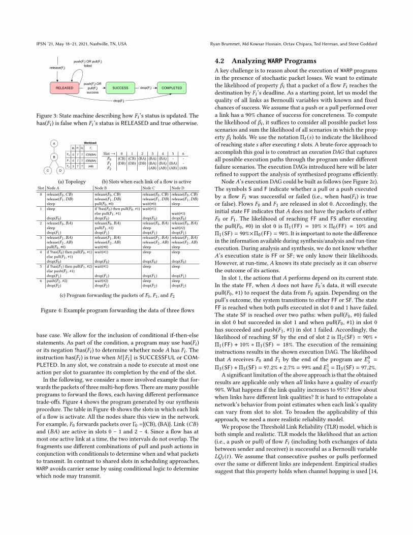
SUCCESSRELEASED COMPLETED
push(Fi) OR pull(Fi) failed
drop(Fi)
release(Fi)
push(Fi) ORpull(Fi)
success
drop(Fi)
Figure 3: State machine describing how 𝐹𝑖 ’s status is updated. The
has(𝐹𝑖 ) is false when 𝐹𝑖 ’s status is RELEASED and true otherwise.
C
B
D
A
F2 (AB)73 7
77 (DB)(BA)F1 0
F0
ϕi Pi Di Γi
0 7 7 (CB)(BA)
Workload:
(a) Topology
Slot→ 0 1 2 3 4 5 6
𝐹0 (CB) (CB) (BA) (BA) (BA) - -
𝐹1 (DB) (DB) (DB) (BA) (BA) (BA) -
𝐹2 (AB) (AB) (AB) (AB)
(b) Slots when each link of a flow is active
Slot Node A Node B Node C Node D
0 release(𝐹0 ,𝐶𝐵) release(𝐹0 ,𝐶𝐵) release(𝐹0 ,𝐶𝐵) release(𝐹0 ,𝐶𝐵)release(𝐹1 , 𝐷𝐵) release(𝐹1 , 𝐷𝐵) release(𝐹1 , 𝐷𝐵) release(𝐹1 , 𝐷𝐵)sleep pull(𝐹0 , #0) wait(#0) sleep
1 sleep if !has(𝐹0) then pull(𝐹0 , #1) wait(#1)else pull(𝐹1 , #1) wait(#1)
drop(𝐹0) drop(𝐹0) drop(𝐹0) drop(𝐹0)2 release(𝐹0 , 𝐵𝐴) release(𝐹0 , 𝐵𝐴) release(𝐹0 , 𝐵𝐴) release(𝐹0 , 𝐵𝐴)
sleep pull(𝐹1 , #2) sleep wait(#2)drop(𝐹1) drop(𝐹1) drop(𝐹1) drop(𝐹1)
3 release(𝐹1 , 𝐵𝐴) release(𝐹1 , 𝐵𝐴) release(𝐹1 , 𝐵𝐴) release(𝐹1 , 𝐵𝐴)release(𝐹2 ,𝐴𝐵) release(𝐹2 ,𝐴𝐵) release(𝐹2 ,𝐴𝐵) release(𝐹2 ,𝐴𝐵)pull(𝐹0 , #0) wait(#0) sleep sleep
4 if !has(𝐹0) then pull(𝐹0 , #1) wait(#1) sleep sleepelse pull(𝐹1 , #1)drop(𝐹0) drop(𝐹0) drop(𝐹0) drop(𝐹0)
5 if !has(𝐹1) then pull(𝐹1 , #2) wait(#1) sleep sleepelse push(𝐹2 , #1)drop(𝐹1) drop(𝐹1) drop(𝐹1) drop(𝐹1)
6 push(𝐹2 , #2) wait(#2) sleep sleepdrop(𝐹2) drop(𝐹2) drop(𝐹2) drop(𝐹2)
(c) Program forwarding the packets of 𝐹0, 𝐹1, and 𝐹2
Figure 4: Example program forwarding the data of three flows
base case. We allow for the inclusion of conditional if-then-else
statements. As part of the condition, a program may use has(𝐹𝑖 )or its negation !has(𝐹𝑖 ) to determine whether node 𝐴 has 𝐹𝑖 . The
instruction has(𝐹𝑖 ) is true when𝑀 [𝐹𝑖 ] is SUCCESSFUL or COM-PLETED. In any slot, we constrain a node to execute at most one
action per slot to guarantee its completion by the end of the slot.
In the following, we consider a more involved example that for-
wards the packets of three multi-hop flows. There are many possible
programs to forward the flows, each having different performance
trade-offs. Figure 4 shows the program generated by our synthesis
procedure. The table in Figure 4b shows the slots in which each link
of a flow is activate. All the nodes share this view in the network.
For example, 𝐹0 forwards packets over Γ0 ={(CB), (BA)}. Link (𝐶𝐵)and (𝐵𝐴) are active in slots 0 – 1 and 2 – 4. Since a flow has at
most one active link at a time, the two intervals do not overlap. The
fragments use different combinations of pull and push actions in
conjunction with conditionals to determine when and what packets
to transmit. In contrast to shared slots in scheduling approaches,
WARP avoids carrier sense by using conditional logic to determine
which node may transmit.
4.2 Analyzing WARP ProgramsA key challenge is to reason about the execution of WARP programs
in the presence of stochastic packet losses. We want to estimate
the likelihood of property 𝛽𝑖 that a packet of a flow 𝐹𝑖 reaches the
destination by 𝐹𝑖 ’s deadline. As a starting point, let us model the
quality of all links as Bernoulli variables with known and fixed
chances of success. We assume that a push or a pull performed over
a link has a 90% chance of success for concreteness. To compute
the likelihood of 𝛽𝑖 , it suffices to consider all possible packet loss
scenarios and sum the likelihood of all scenarios in which the prop-
erty 𝛽𝑖 holds. We use the notation Π𝑡 (𝑠) to indicate the likelihood
of reaching state 𝑠 after executing 𝑡 slots. A brute-force approach to
accomplish this goal is to construct an execution DAG that captures
all possible execution paths through the program under different
failure scenarios. The execution DAGs introduced here will be later
refined to support the analysis of synthesized programs efficiently.
Node𝐴’s execution DAG could be built as follows (see Figure 2c).
The symbols S and F indicate whether a pull or a push executed
by a flow 𝐹𝑖 was successful or failed (i.e., when has(𝐹𝑖 ) is trueor false). Flows 𝐹0 and 𝐹1 are released in slot 0. Accordingly, the
initial state FF indicates that 𝐴 does not have the packets of either
𝐹0 or 𝐹1. The likelihood of reaching FF and FS after executing
the pull(𝐹0, #0) in slot 0 is Π1 (FF) = 10% × Π0 (FF) = 10% and
Π1 (SF) = 90%×Π0 (FF) = 90%. It is important to note the difference
in the information available during synthesis/analysis and run-time
execution. During analysis and synthesis, we do not know whether
𝐴’s execution state is FF or SF; we only know their likelihoods.
However, at run-time, 𝐴 knows its state precisely as it can observe
the outcome of its actions.
In slot 1, the actions that 𝐴 performs depend on its current state.
In the state FF, when 𝐴 does not have 𝐹0’s data, it will execute
pull(𝐹0, #1) to request the data from 𝐹0 again. Depending on the
pull’s outcome, the system transitions to either FF or SF. The stateFF is reached when both pulls executed in slot 0 and 1 have failed.
The state SF is reached over two paths: when pull(𝐹0, #0) failedin slot 0 but succeeded in slot 1 and when pull(𝐹0, #1) in slot 0
has succeeded and push(𝐹1, #1) in slot 1 failed. Accordingly, the
likelihood of reaching SF by the end of slot 2 is Π2 (SF) = 90% ∗Π1 (FF) + 10% ∗ Π1 (SF) = 18%. The execution of the remaining
instructions results in the shown execution DAG. The likelihood
that 𝐴 receives 𝐹0 and 𝐹1 by the end of the program are 𝐸03=
Π3 (SF) + Π3 (SF) = 97.2% + 2.7% = 99% and 𝐸13= Π3 (SF) = 97.2%.
A significant limitation of the above approach is that the obtained
results are applicable only when all links have a quality of exactly90%. What happens if the link quality increases to 95%? How about
when links have different link qualities? It is hard to extrapolate a
network’s behavior from point estimates when each link’s quality
can vary from slot to slot. To broaden the applicability of this
approach, we need a more realistic reliability model.
We propose the Threshold Link Reliability (TLR) model, which is
both simple and realistic. TLR models the likelihood that an action
(i.e., a push or pull) of flow 𝐹𝑖 (including both exchanges of data
between sender and receiver) is successful as a Bernoulli variable
𝐿𝑄𝑖 (𝑡). We assume that consecutive pushes or pulls performed
over the same or different links are independent. Empirical studies
suggest that this property holds when channel hopping is used [14,
WARP: On-the-fly Program Synthesis for Agile, Real-time, and Reliable Wireless Networks IPSN ’21, May 18–21, 2021, Nashville, TN, USA
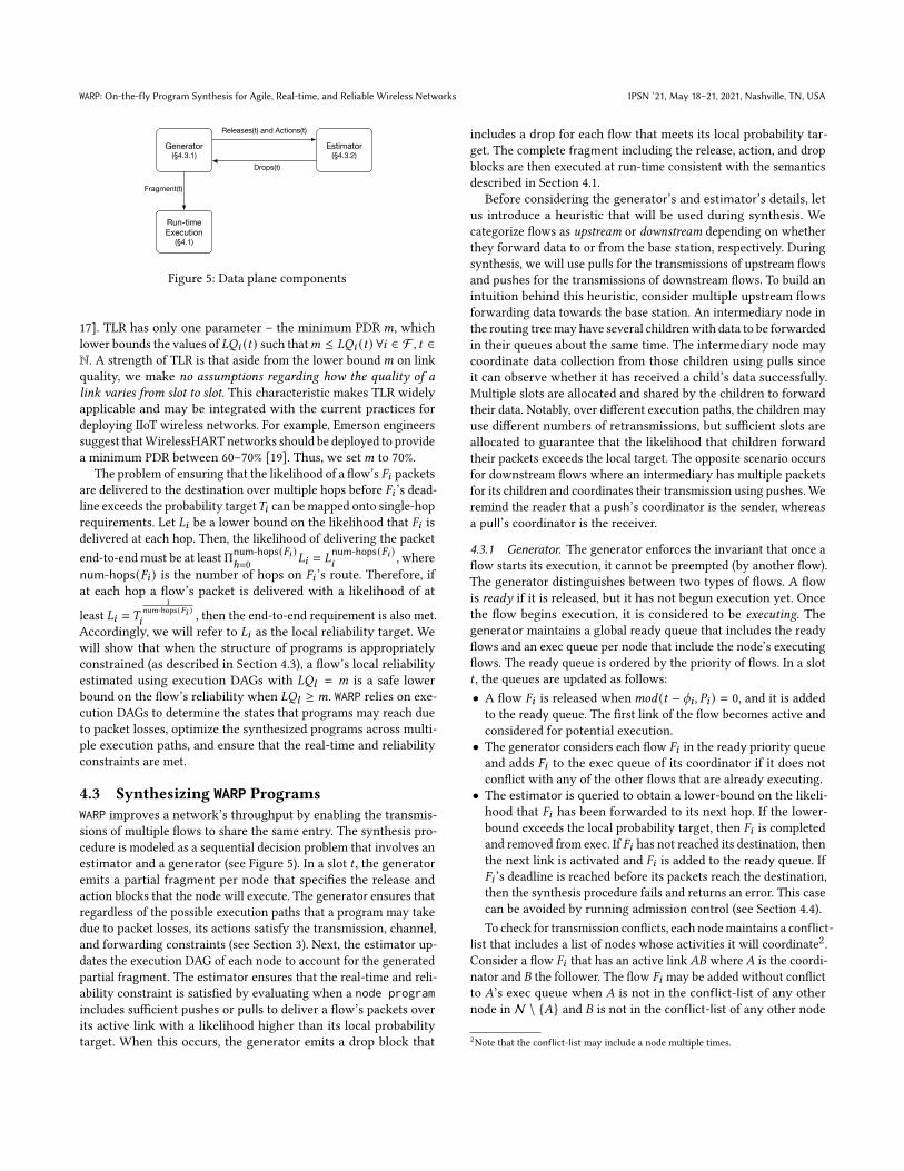
Generator(§4.3.1)
Estimator(§4.3.2)
Releases(t) and Actions(t)
Drops(t)
Run-timeExecution
(§4.1)
Fragment(t)
Figure 5: Data plane components
17]. TLR has only one parameter – the minimum PDR𝑚, which
lower bounds the values of 𝐿𝑄𝑖 (𝑡) such that𝑚 ≤ 𝐿𝑄𝑖 (𝑡) ∀𝑖 ∈ F , 𝑡 ∈N. A strength of TLR is that aside from the lower bound𝑚 on link
quality, we make no assumptions regarding how the quality of alink varies from slot to slot. This characteristic makes TLR widely
applicable and may be integrated with the current practices for
deploying IIoT wireless networks. For example, Emerson engineers
suggest thatWirelessHART networks should be deployed to provide
a minimum PDR between 60–70% [19]. Thus, we set𝑚 to 70%.
The problem of ensuring that the likelihood of a flow’s 𝐹𝑖 packets
are delivered to the destination over multiple hops before 𝐹𝑖 ’s dead-
line exceeds the probability target𝑇𝑖 can be mapped onto single-hop
requirements. Let 𝐿𝑖 be a lower bound on the likelihood that 𝐹𝑖 is
delivered at each hop. Then, the likelihood of delivering the packet
end-to-end must be at least Πnum-hops(𝐹𝑖 )ℎ=0
𝐿𝑖 = 𝐿num-hops(𝐹𝑖 )𝑖
, where
num-hops(𝐹𝑖 ) is the number of hops on 𝐹𝑖 ’s route. Therefore, if
at each hop a flow’s packet is delivered with a likelihood of at
least 𝐿𝑖 = 𝑇
1
num-hops(𝐹𝑖 )𝑖
, then the end-to-end requirement is also met.
Accordingly, we will refer to 𝐿𝑖 as the local reliability target. We
will show that when the structure of programs is appropriately
constrained (as described in Section 4.3), a flow’s local reliability
estimated using execution DAGs with 𝐿𝑄𝑙 = 𝑚 is a safe lower
bound on the flow’s reliability when 𝐿𝑄𝑙 ≥ 𝑚. WARP relies on exe-
cution DAGs to determine the states that programs may reach due
to packet losses, optimize the synthesized programs across multi-
ple execution paths, and ensure that the real-time and reliability
constraints are met.
4.3 Synthesizing WARP ProgramsWARP improves a network’s throughput by enabling the transmis-
sions of multiple flows to share the same entry. The synthesis pro-
cedure is modeled as a sequential decision problem that involves an
estimator and a generator (see Figure 5). In a slot 𝑡 , the generatoremits a partial fragment per node that specifies the release and
action blocks that the node will execute. The generator ensures thatregardless of the possible execution paths that a program may take
due to packet losses, its actions satisfy the transmission, channel,
and forwarding constraints (see Section 3). Next, the estimator up-dates the execution DAG of each node to account for the generated
partial fragment. The estimator ensures that the real-time and reli-
ability constraint is satisfied by evaluating when a node programincludes sufficient pushes or pulls to deliver a flow’s packets over
its active link with a likelihood higher than its local probability
target. When this occurs, the generator emits a drop block that
includes a drop for each flow that meets its local probability tar-
get. The complete fragment including the release, action, and drop
blocks are then executed at run-time consistent with the semantics
described in Section 4.1.
Before considering the generator’s and estimator’s details, letus introduce a heuristic that will be used during synthesis. We
categorize flows as upstream or downstream depending on whether
they forward data to or from the base station, respectively. During
synthesis, we will use pulls for the transmissions of upstream flows
and pushes for the transmissions of downstream flows. To build an
intuition behind this heuristic, consider multiple upstream flows
forwarding data towards the base station. An intermediary node in
the routing treemay have several childrenwith data to be forwarded
in their queues about the same time. The intermediary node may
coordinate data collection from those children using pulls sinceit can observe whether it has received a child’s data successfully.
Multiple slots are allocated and shared by the children to forward
their data. Notably, over different execution paths, the children may
use different numbers of retransmissions, but sufficient slots are
allocated to guarantee that the likelihood that children forward
their packets exceeds the local target. The opposite scenario occurs
for downstream flows where an intermediary has multiple packets
for its children and coordinates their transmission using pushes. We
remind the reader that a push’s coordinator is the sender, whereasa pull’s coordinator is the receiver.
4.3.1 Generator. The generator enforces the invariant that once aflow starts its execution, it cannot be preempted (by another flow).
The generator distinguishes between two types of flows. A flow
is ready if it is released, but it has not begun execution yet. Once
the flow begins execution, it is considered to be executing. Thegenerator maintains a global ready queue that includes the ready
flows and an exec queue per node that include the node’s executingflows. The ready queue is ordered by the priority of flows. In a slot
𝑡 , the queues are updated as follows:
• A flow 𝐹𝑖 is released when𝑚𝑜𝑑 (𝑡 − 𝜙𝑖 , 𝑃𝑖 ) = 0, and it is added
to the ready queue. The first link of the flow becomes active and
considered for potential execution.
• The generator considers each flow 𝐹𝑖 in the ready priority queueand adds 𝐹𝑖 to the exec queue of its coordinator if it does notconflict with any of the other flows that are already executing.
• The estimator is queried to obtain a lower-bound on the likeli-
hood that 𝐹𝑖 has been forwarded to its next hop. If the lower-
bound exceeds the local probability target, then 𝐹𝑖 is completed
and removed from exec. If 𝐹𝑖 has not reached its destination, thenthe next link is activated and 𝐹𝑖 is added to the ready queue. If
𝐹𝑖 ’s deadline is reached before its packets reach the destination,
then the synthesis procedure fails and returns an error. This case
can be avoided by running admission control (see Section 4.4).
To check for transmission conflicts, each nodemaintains a conflict-list that includes a list of nodes whose activities it will coordinate2.Consider a flow 𝐹𝑖 that has an active link 𝐴𝐵 where 𝐴 is the coordi-
nator and 𝐵 the follower. The flow 𝐹𝑖 may be added without conflict
to 𝐴’s exec queue when 𝐴 is not in the conflict-list of any other
node in N \ {𝐴} and 𝐵 is not in the conflict-list of any other node
2Note that the conflict-list may include a node multiple times.
IPSN ’21, May 18–21, 2021, Nashville, TN, USA Ryan Brummet, Md Kowsar Hossain, Octav Chipara, Ted Herman, and Steve Goddard
inN \ {𝐴, 𝐵}. In this is the case, 𝐹𝑖 is added to𝐴’s exec queue and 𝐵is added to𝐴’s conflict-list. When a flow 𝐹𝑖 completes its execution,
𝐵 is removed from its conflict-list. By choosing appropriate data
structures, we can construct a generator that runs in 𝑂 ( |F |).The generator produces the next fragment of a node program
based on the node’s exec queue. A fragment includes a release
block, an action block, and a drop block. The release block includes
all the flows that have been released in the current slot. The drop
block includes all flows that the estimator determined to have met
their local probability target. Note that since release and drop are
global events, they are included in all nodes’ fragments, so they
have a consistent view of when flows are released and dropped. If
the exec queue is empty, an action block that includes a single sleepis generated. When there is a single flow in exec, either a push or a
pull is generated depending on whether the flow is downstream or
upstream, respectively. The actionwill use a channel that is assigned
by the coordinator. Each coordinator maintains a counter that is
initialized with a common random number and is incremented
each time it executes a push or a pull. The assigned channel is the
modulus of the counter and the maximum number of channels.
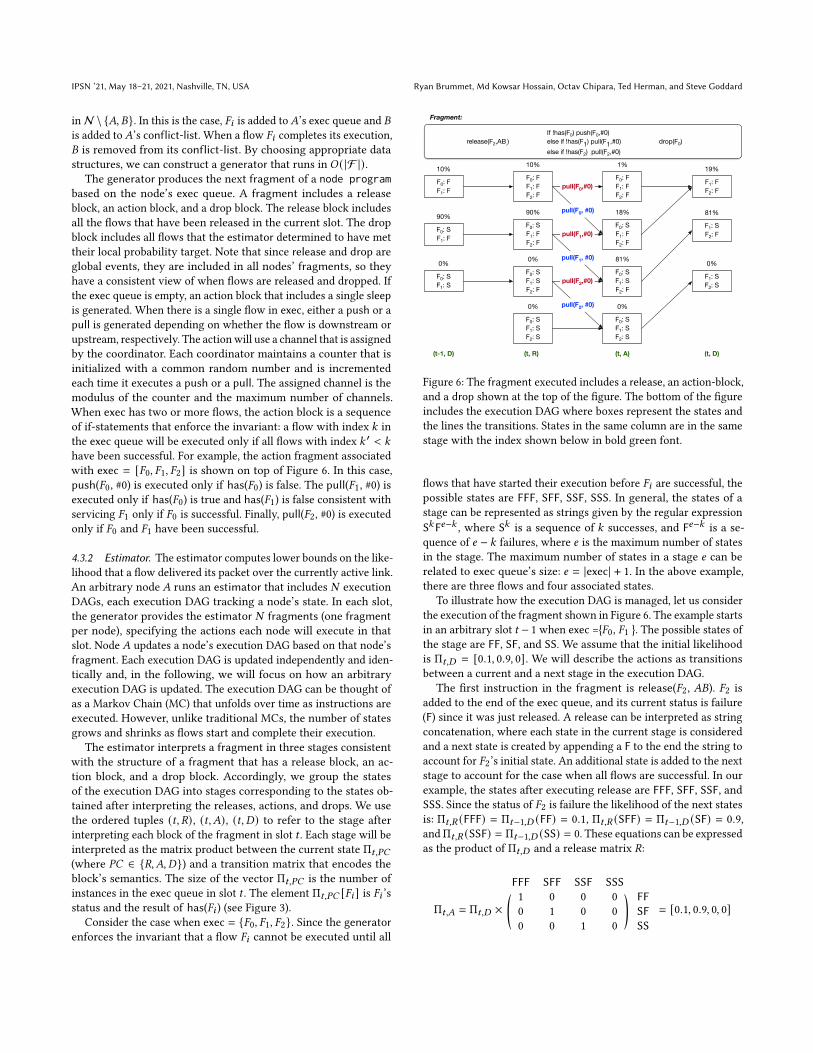
When exec has two or more flows, the action block is a sequence
of if-statements that enforce the invariant: a flow with index 𝑘 in
the exec queue will be executed only if all flows with index 𝑘 ′ < 𝑘
have been successful. For example, the action fragment associated
with exec = [𝐹0, 𝐹1, 𝐹2] is shown on top of Figure 6. In this case,
push(𝐹0, #0) is executed only if has(𝐹0) is false. The pull(𝐹1, #0) isexecuted only if has(𝐹0) is true and has(𝐹1) is false consistent withservicing 𝐹1 only if 𝐹0 is successful. Finally, pull(𝐹2, #0) is executedonly if 𝐹0 and 𝐹1 have been successful.
4.3.2 Estimator. The estimator computes lower bounds on the like-
lihood that a flow delivered its packet over the currently active link.
An arbitrary node 𝐴 runs an estimator that includes 𝑁 execution
DAGs, each execution DAG tracking a node’s state. In each slot,
the generator provides the estimator 𝑁 fragments (one fragmentper node), specifying the actions each node will execute in that
slot. Node 𝐴 updates a node’s execution DAG based on that node’s
fragment. Each execution DAG is updated independently and iden-
tically and, in the following, we will focus on how an arbitrary
execution DAG is updated. The execution DAG can be thought of
as a Markov Chain (MC) that unfolds over time as instructions are
executed. However, unlike traditional MCs, the number of states
grows and shrinks as flows start and complete their execution.
The estimator interprets a fragment in three stages consistent
with the structure of a fragment that has a release block, an ac-
tion block, and a drop block. Accordingly, we group the states
of the execution DAG into stages corresponding to the states ob-
tained after interpreting the releases, actions, and drops. We use
the ordered tuples (𝑡, 𝑅), (𝑡, 𝐴), (𝑡, 𝐷) to refer to the stage after
interpreting each block of the fragment in slot 𝑡 . Each stage will be
interpreted as the matrix product between the current state Π𝑡,𝑃𝐶
(where 𝑃𝐶 ∈ {𝑅,𝐴, 𝐷}) and a transition matrix that encodes the
block’s semantics. The size of the vector Π𝑡,𝑃𝐶 is the number of
instances in the exec queue in slot 𝑡 . The element Π𝑡,𝑃𝐶 [𝐹𝑖 ] is 𝐹𝑖 ’sstatus and the result of has(𝐹𝑖 ) (see Figure 3).
Consider the case when exec = {𝐹0, 𝐹1, 𝐹2}. Since the generatorenforces the invariant that a flow 𝐹𝑖 cannot be executed until all
F0: FF1: F
10%
F0: SF1: F
90%
F0: SF1: S
0%
F0: FF1: FF2: F
10%
F0: SF1: FF2: F
90%
F0: SF1: SF2: F
0%
F0: SF1: SF2: S
0%
release(F2,AB,)
F0: FF1: FF2: F
1%
F0: SF1: FF2: F
18%
F0: SF1: SF2: F
81%
F0: SF1: SF2: S
0%
If !has(F0) push(F0,#0)else if !has(F1) pull(F1,#0)else if !has(F2) pull(F2,#0)
pull(F0,#0)
pull(F0, #0)
pull(F1,#0)
pull(F2,#0)
pull(F1, #0)
pull(F2, #0)
drop(F0)
F1: FF2: F
19%
F1: SF2: F
81%
F1: SF2: S
0%
Fragment:
(t-1, D) (t, R) (t, A) (t, D)
Figure 6: The fragment executed includes a release, an action-block,
and a drop shown at the top of the figure. The bottom of the figure
includes the execution DAG where boxes represent the states and
the lines the transitions. States in the same column are in the same
stage with the index shown below in bold green font.
flows that have started their execution before 𝐹𝑖 are successful, the
possible states are FFF, SFF, SSF, SSS. In general, the states of a
stage can be represented as strings given by the regular expression
S𝑘F𝑒−𝑘 , where S𝑘 is a sequence of 𝑘 successes, and F𝑒−𝑘 is a se-
quence of 𝑒 − 𝑘 failures, where 𝑒 is the maximum number of states
in the stage. The maximum number of states in a stage 𝑒 can be
related to exec queue’s size: 𝑒 = |exec| + 1. In the above example,
there are three flows and four associated states.
To illustrate how the execution DAG is managed, let us consider
the execution of the fragment shown in Figure 6. The example starts
in an arbitrary slot 𝑡 − 1 when exec ={𝐹0, 𝐹1 }. The possible states ofthe stage are FF, SF, and SS. We assume that the initial likelihood
is Π𝑡,𝐷 = [0.1, 0.9, 0]. We will describe the actions as transitions
between a current and a next stage in the execution DAG.
The first instruction in the fragment is release(𝐹2, 𝐴𝐵). 𝐹2 is
added to the end of the exec queue, and its current status is failure
(F) since it was just released. A release can be interpreted as string
concatenation, where each state in the current stage is considered
and a next state is created by appending a F to the end the string toaccount for 𝐹2’s initial state. An additional state is added to the next
stage to account for the case when all flows are successful. In our
example, the states after executing release are FFF, SFF, SSF, andSSS. Since the status of 𝐹2 is failure the likelihood of the next statesis: Π𝑡,𝑅 (FFF) = Π𝑡−1,𝐷 (FF) = 0.1, Π𝑡,𝑅 (SFF) = Π𝑡−1,𝐷 (SF) = 0.9,
andΠ𝑡,𝑅 (SSF) = Π𝑡−1,𝐷 (SS) = 0. These equations can be expressed
as the product of Π𝑡,𝐷 and a release matrix 𝑅:
Π𝑡,𝐴 = Π𝑡,𝐷 ×
FFF SFF SSF SSS( )1 0 0 0 FF0 1 0 0 SF0 0 1 0 SS
= [0.1, 0.9, 0, 0]
WARP: On-the-fly Program Synthesis for Agile, Real-time, and Reliable Wireless Networks IPSN ’21, May 18–21, 2021, Nashville, TN, USA
In general, a release is interpreted as the product of the current
state and a release matrix 𝑅 of size 𝑒 × (𝑒 +1). All rows 𝑟 of a releasematrix 𝑅 have a single non-zero entry 𝑅 [𝑟, 𝑟 ] = 1 for 0 ≤ 𝑟 < 𝑒 .
Next, we consider the action block of the fragment and generatea transition matrix 𝐴 that accounts for the entire block’s execution.
Let 𝐿𝑄𝑡 be the chance that the packets associated with the selected
action are transmitted successfully. 𝐿𝑄𝑡 is 90% in our example. Flow
𝐹0 is executed only in state FFF since it is the only state in which
!has(𝐹0) is true. If the action fails, the system remains in the same
with the likelihood 1−𝐿𝑄𝑡 ; otherwise, it transitions to the state SFFwith likelihood 𝐿𝑄𝑡 . Flow 𝐹1 is executed only in state SFF when
has(𝐹0) is false (i.e., 𝐹0’s status is success) and !has(𝐹1) is false. Uponits execution, the system transitions to state SFF with likelihood
1 − 𝐿𝑄𝑡 and transitions to state SSF with likelihood 𝐿𝑄𝑡 . Similarly,
𝐹2 is executed in state SSF, causing the system to remain in state
SSFwith likelihood 1−𝐿𝑄𝑡 or transition to SSSwith likelihood 𝐿𝑄𝑡 .
Finally, no flow is executed in state SSS and the system remains in
this state with a likelihood of 1. The execution of the actions can
be accounted for according to the following matrix multiplication:
Π𝑡,𝐷 = Π𝑡,𝑅 ×
FFF SFF SSF SSS©«ª®®¬
1 − 𝐿𝑄𝑡 𝐿𝑄𝑡 0 0 FFF0 1 − 𝐿𝑄𝑡 𝐿𝑄𝑡 0 SFF0 0 1 − 𝐿𝑄𝑡 𝐿𝑄𝑡 SSF0 0 0 1 SSS
= [0.01, 0.18, 0.81, 0]
In general, the actions block can be represented as a matrix 𝐴 of
size 𝑒 × 𝑒 . All rows 𝑟 such that 𝑟 < 𝑒 − 1 have two non-zero entries:
𝐴[𝑟, 𝑟 ] = 1 −𝑚 and 𝐴[𝑟, 𝑟 + 1] =𝑚. The last row has all elements
zero except the last column, which is 1.
A drop(𝐹0) indicates that 𝐹0 has finished executing and is locatedat the head of the exec queue. Similar to the release instruction, the
drop can also be treated as a string operation that considers each
state and generates a new state by removing the left-most character.
This results in the first two states having the same suffix and their
likelihoods are added when generating the single combined new
state. In our example, removing the first character of maps states
FFF and FSS on the same state FF. Thus, Π𝑡,𝐷 (FF) = Π𝑡,𝐴 (FFF) +Π𝑡,𝐴 (SFF). For the rest of the states, Π𝑡,𝐷 (SF) = Π𝑡,𝐴 (SSF) andΠ𝑡,𝐷 (SS) = Π𝑡,𝐴 (SSS). These equations can be specified as the
following matrix product:
Π𝑡,𝑅 = Π𝑡,𝐷 ×
FF SF SS©«ª®®¬
1 0 0 FFF1 0 0 SFF0 1 0 SSF0 0 1 SSS
= [0.19, 0.81, 0]
In general, interpreting a drop involves multiplying the current
state with a matrix 𝐷 . Each row of 𝐷 has a single non-zero entry
that is one. The first row the non-zero entry is𝐷 [1, 1] = 1 and in the
remaining rows 𝑟 (1 ≤ 𝑟 < 𝑒) the non-zero entry is 𝐷 [𝑟, 𝑟 − 1] = 1.
Let 𝐸𝑖𝑡 be the likelihood that flow 𝐹𝑖 forwarded its packets by
slot 𝑡 . The local reliability of a flow 𝐹𝑖 may then computed as the
sum of all the states where the flow was successful. In our example,
𝐸0𝑡 = Π𝑡,𝐴 [SFF] + Π𝑡,𝐴 [SSF] + Π𝑡,𝐴 [SSS] = 0.99.
The TLR model allows the quality of links to vary from slot
to slot arbitrarily as long as it exceeds a minimum link quality
𝑚. The reliability of a flow 𝐹𝑖 is a function 𝐸𝑖𝑡 (𝐿𝑄0, 𝐿𝑄1, . . . 𝐿𝑄𝑡 )that depends on the 𝐿𝑄𝑡 , which is likelihood that the the pull orpush in slot 𝑡 succeeds. We claim that a lower bound 𝐸𝑖𝑡 (𝑚) may
be computed by setting 𝐿𝑄𝑡 equal to the𝑚 in all matrices A that
encode action blocks:
𝐸𝑖𝑡 (𝑚) = 𝐸𝑡𝑖 (𝐿𝑄0 =𝑚, 𝐿𝑄1 =𝑚, . . . 𝐿𝑄𝑡 =𝑚) ≤ 𝐸𝑡𝑖 (𝐿𝑄0, 𝐿𝑄1, . . . 𝐿𝑄𝑡 )
Theorem 4.1. Consider a node A and a set of flows F𝐴 =
{𝐹0, 𝐹1, ..𝐹𝑀 } such that A is as either a source or a destination ofthe 𝐹𝑖 ’s active link (𝐹𝑖 ∈ F𝐴). Let 𝐿𝑄𝑡 be the likelihood that the pushor pull performed in slot 𝑡 succeeds such that𝑚 ≤ 𝐿𝑄𝑡 ≤ 1 for allslots t (𝑡 ∈ N) The local reliability 𝐸𝑖𝑡 (𝐿𝑄0, 𝐿𝑄1, . . . 𝐿𝑄𝑡 ) that 𝐹𝑖 ’spackets are delivered over its active link is lower-bounded by 𝐸𝑖𝑡 (𝑚).
Proof. Due to space limits, the proof is included in [5]. □
Due to the structure of the synthesized code, the execution DAGs
can be managed very efficiently. The number of states in the execu-
tion DAG is |exec| + 1, each state requiring one floating-point per
state. To control the storage and computational requirements, we
have modified the generator to move an instance from the readyto the exec queue only if the exec queue’s size is below a thresh-
old. Experiments show that setting this threshold to four entries
provides significant performance gains while introducing a small
memory and computational overhead. Specifically, we require that
a device maintain 5 × 𝑁 floating-points. A potential challenge with
implementing the execution DAG using matrix multiplication is
that floating-point operations tend to be slow or unsupported on
embedded devices. Our implementation avoids matrix multiplica-
tion altogether and further reduces memory usage by converting
multiplications into table look-ups. We divide the interval [0, 1] ofpotential values into a small number of intervals. Since the tran-
sition matrix only depends on the parameter𝑚 of TLR, we cache
the results of multiplying each interval with𝑚. Our experiments
indicate that caching a small number of values provides a good
approximation of a flow’s reliability.
4.4 Control PlaneWARP uses a control plane similar to REACT’s [15] and, in the fol-
lowing, we will primarily highlight those differences. The unique
aspect of WARP is that it does not disseminate programs. Instead,
WARP disseminates the workload and topology changes, and nodes
independently reconstruct a shared schedule. A workload change
is initiated either by the network operator or by a node within
the network, sending a request to the base station to add, remove,
or modify a flow. A topology change is detected by the network
manager based on the periodic health reports provided by nodes.
In either case, WARP runs admission control to ensure that a fea-
sible program may be generated. If a program is not synthesized
successfully, then rate control techniques are applied to reduce
the workload. Due to the efficiency of our synthesis procedure,
the overhead of doing so is minimal. If a program is synthesized,
then WARP disseminates the topology and workload changes to all
IPSN ’21, May 18–21, 2021, Nashville, TN, USA Ryan Brummet, Md Kowsar Hossain, Octav Chipara, Ted Herman, and Steve Goddard
nodes which then synthesize the program. We use a broadcast tree
mechanism proposed in REACT to disseminate the topology and/or
workload changes.
Changes in workload and topology may be encoded and dissemi-
nated efficiently. The addition of a new flow requires disseminating
its associated parameters: a flow identifier, phase, period, deadline,
priority, and route. There are a small number of classes in most
applications, each class having its temporal parameters and priority
level. Accordingly, we can avoid disseminating the temporal and
priority of a flow and simply disseminating the class’s identifier for
the flow. Similarly, rather than disseminating a route, it suffices to
use a route identifier that refers to a route in the table maintained
by the node. Accordingly, to add a flow, it suffices to transmit a
total of 4 bytes – 2 for the identifier, 1 for the flow class, and 1 for
the route identifier. A command to remove the flow only requires
passing the identifier of the flow to be removed. Changes to the
routing information can also be encoded efficiently. The operations
that are allowed on the routing table is to add, duplicate, modify,
or delete routes. A common case is for a link to change, requiring
several routes to be modified. WARP handles this use case using a
modify command that treats each route as a string and performs
a search and replace operation. The key behind this approach’s
efficiency is that the operation is applied to all routes in the table.
5 EXPERIMENTSOur experiments answer the following questions:
• Does WARP improve the throughput in typical IIoT workloads?
• Can WARP run on resource-constrained embedded devices?
• How agile is WARP’s control plane to workload changes?
• Can WARP satisfy the real-time and reliability constraints and
adapt to fluctuations in link quality?
We compare WARP against three baselines: CLLF, REACT, andRecorp.CLLF is a heuristic approach to building near-optimal sched-
ules [23]. REACT improves the agility of control planes by constrain-
ing the construction of schedules such that they are easier to update
in response to workload and topology changes. In response to a
workload change, CLLF and REACT disseminate only the differ-
ences between the current and updated schedules. Recorp uses
an SMT solver to constructs policies that can share slots across
multiple flows. However, Recorp can take as long as a minute to
construct policies and uses a centralized control plane. We con-
sidered two versions of WARP— WARP and WARP*. WARP’s estimator
uses matrix operations while WARP* converts matrix operations to
table lookups to avoid floating-point operations. WARP*’s lookuptable is configured to use 527 bytes to balance memory usage and
performance. As the lookup table’s size increases, the difference in
the performance of WARP and WARP* decreases.We set𝑚 = 70%, as suggested by Emerson’s guide to deploying
WirelessHART networks. In simulations, we set the probability of a
successful transmission to equal𝑚. The number of transmissions for
all protocols is set to achieve 99% end-to-end reliability for all flows.
Each experiment considers a different workload. However, a flow’s
period and deadline are equal, and its phase is zero in all workloads.
Except for CLLF, which uses a heuristic to assign priorities, flow
priorities are assigned such that flows with shorter deadlines have
higher priority. Additionally, flows with longer routes have a higher
priority and remaining ties are broken arbitrarily.
We quantified the performance of protocols using total through-
put, synthesis time, control overhead, and consensus time. The
total throughput is the maximum number of packets per second
that flows can deliver without missing the real-time or reliability
constraints. Synthesis time is the amount of time needed to synthe-
size programs or construct schedules. The control plane’s agility is
quantified by the number of bytes used for control overhead and
the consensus time until all nodes update the program or schedule
in response to a workload change.
5.1 SimulationsWe have performed simulations on two real topologies: the Indriya
topology which includes 85 nodes and has a 6-hop diameter (Indriya
topology) [9], and the Washington Universtiy in St. Louis topology
which includes includes 41 nodes and has a 6-hop diameter (WashU
topology) [1]. The simulations use 802.15.4 with 16 channels.
To provide a comprehensive comparison between protocols, we
considered three typical workloads under a multihop topology:
data collection, data dissemination, and a mix of data collection
and dissemination. The results presented are obtained from 100
simulation runs per workload type. In all runs, the base station is
selected as the closest node to the topology center. In each run, 50
flows are created with the following constraints:
• Data Collection (COL): Sources are selected randomly with the
base station as the destination.
• Data Dissemination (DIS): The base station is the source, and
destinations are randomly selected.
• Data Collection and Dissemination (MIX): Each flow is randomly
selected to use either COL or DIS.Each flow is randomly assigned to one of three classes whose peri-
ods and deadlines maintain a 1:2:5 ratio. Accordingly, if Class 1 isassigned a period of 100𝑚𝑠 , then Class 2 is assigned 200𝑚𝑠 , and
Class 3 500𝑚𝑠 . We call the period of Class 1 the base period. Ineach run, the base period is decreased until a deadline is missed.
The following results are obtained for the smallest base period for
which all flows met their deadlines.
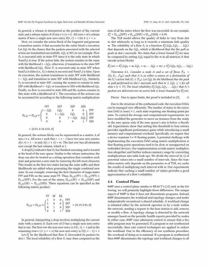
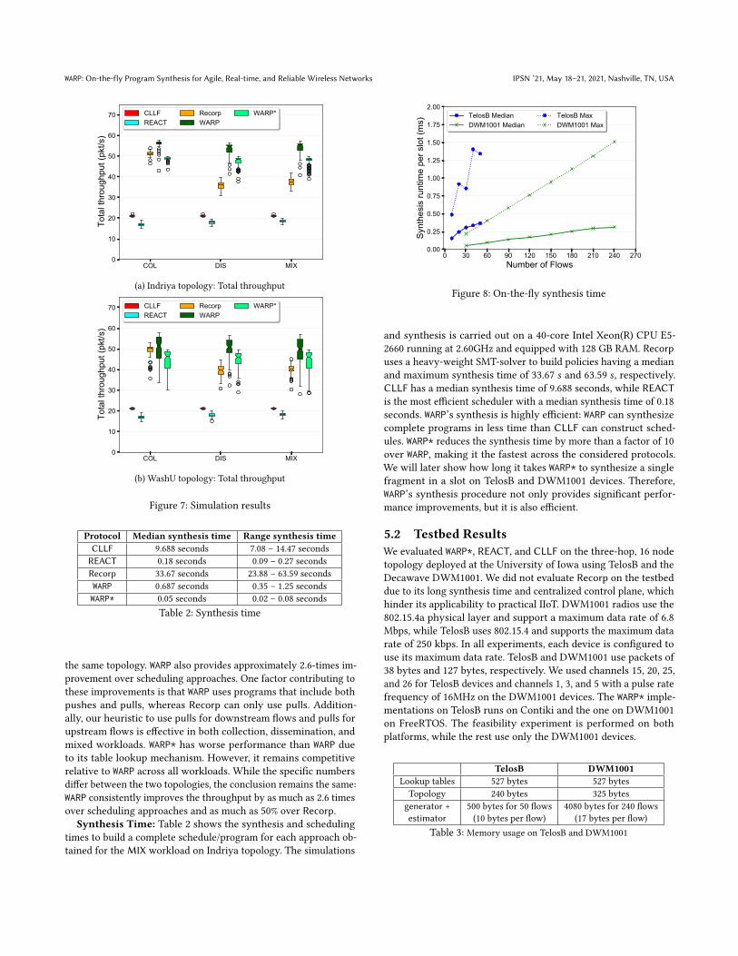
Flow throughput: Figures 7a and 7b plot the total throughput
of each protocol under the considered workload type for the two
topologies. We observed the same trend in both topologies: CLLFand REACT have significantly lower throughput than Recorp, WARP,and WARP*. REACT has a slightly lower median throughput than
CLLF because its gap-induced algorithm forces all instances of a
flow to have the same repeating pattern of transmissions. The clear
winners are Recorp, WARP, and WARP*, because they can share en-
tries across multiple flows, significantly improving the supported
throughput. However, Recorp’s performance varies significantly
across different workload types. WARP improves upon Recorp’s me-
dian throughput across all scenarios, with notable improvements for
the DIS andMIX scenarios. In the Indriya topology forMIX work-
loads, WARP supports a medium total throughput of 55.4 packets per
second compared to Recorp’s 37.5 packets per second, represent-ing a 47.68% improvement in throughput over Recorp. A slightly
larger improvement of 52% is observed for the DIS workload in
WARP: On-the-fly Program Synthesis for Agile, Real-time, and Reliable Wireless Networks IPSN ’21, May 18–21, 2021, Nashville, TN, USA
COL DIS MIX0
10
20
30
40
50
60
70
Tota
l thr
ough
put (
pkt/s
)CLLFREACT
RecorpWARP
WARP*
(a) Indriya topology: Total throughput
COL DIS MIX0
10
20
30
40
50
60
70
Tota
l thr
ough
put (
pkt/s
)
CLLFREACT
RecorpWARP
WARP*
(b) WashU topology: Total throughput
Figure 7: Simulation results
Protocol Median synthesis time Range synthesis timeCLLF 9.688 seconds 7.08 – 14.47 seconds
REACT 0.18 seconds 0.09 – 0.27 seconds
Recorp 33.67 seconds 23.88 – 63.59 seconds
WARP 0.687 seconds 0.35 – 1.25 seconds
WARP* 0.05 seconds 0.02 – 0.08 seconds
Table 2: Synthesis time
the same topology. WARP also provides approximately 2.6-times im-
provement over scheduling approaches. One factor contributing to
these improvements is that WARP uses programs that include both
pushes and pulls, whereas Recorp can only use pulls. Addition-ally, our heuristic to use pulls for downstream flows and pulls forupstream flows is effective in both collection, dissemination, and
mixed workloads. WARP* has worse performance than WARP due
to its table lookup mechanism. However, it remains competitive
relative to WARP across all workloads. While the specific numbers
differ between the two topologies, the conclusion remains the same:
WARP consistently improves the throughput by as much as 2.6 times
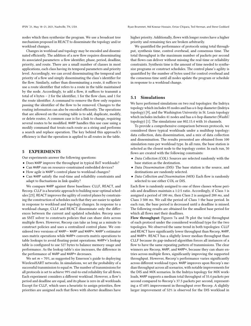
over scheduling approaches and as much as 50% over Recorp.Synthesis Time: Table 2 shows the synthesis and scheduling
times to build a complete schedule/program for each approach ob-
tained for the MIX workload on Indriya topology. The simulations
0 30 60 90 120 150 180 210 240 270Number of Flows
0.00
0.25
0.50
0.75
1.00
1.25
1.50
1.75
2.00
Syn
thes
is ru
ntim
e pe
r slo
t (m
s)
TelosB MedianDWM1001 Median
TelosB MaxDWM1001 Max
Figure 8: On-the-fly synthesis time
and synthesis is carried out on a 40-core Intel Xeon(R) CPU E5-
2660 running at 2.60GHz and equipped with 128 GB RAM. Recorpuses a heavy-weight SMT-solver to build policies having a median
and maximum synthesis time of 33.67 𝑠 and 63.59 𝑠 , respectively.
CLLF has a median synthesis time of 9.688 seconds, while REACTis the most efficient scheduler with a median synthesis time of 0.18
seconds. WARP’s synthesis is highly efficient: WARP can synthesize
complete programs in less time than CLLF can construct sched-
ules. WARP* reduces the synthesis time by more than a factor of 10
over WARP, making it the fastest across the considered protocols.
We will later show how long it takes WARP* to synthesize a single
fragment in a slot on TelosB and DWM1001 devices. Therefore,
WARP’s synthesis procedure not only provides significant perfor-
mance improvements, but it is also efficient.
5.2 Testbed ResultsWe evaluated WARP*, REACT, and CLLF on the three-hop, 16 node
topology deployed at the University of Iowa using TelosB and the
Decawave DWM1001. We did not evaluate Recorp on the testbed
due to its long synthesis time and centralized control plane, which
hinder its applicability to practical IIoT. DWM1001 radios use the
802.15.4a physical layer and support a maximum data rate of 6.8
Mbps, while TelosB uses 802.15.4 and supports the maximum data
rate of 250 kbps. In all experiments, each device is configured to
use its maximum data rate. TelosB and DWM1001 use packets of
38 bytes and 127 bytes, respectively. We used channels 15, 20, 25,
and 26 for TelosB devices and channels 1, 3, and 5 with a pulse rate
frequency of 16MHz on the DWM1001 devices. The WARP* imple-
mentations on TelosB runs on Contiki and the one on DWM1001
on FreeRTOS. The feasibility experiment is performed on both
platforms, while the rest use only the DWM1001 devices.
TelosB DWM1001Lookup tables 527 bytes 527 bytes
Topology 240 bytes 325 bytes
generator + 500 bytes for 50 flows 4080 bytes for 240 flows
estimator (10 bytes per flow) (17 bytes per flow)
Table 3: Memory usage on TelosB and DWM1001
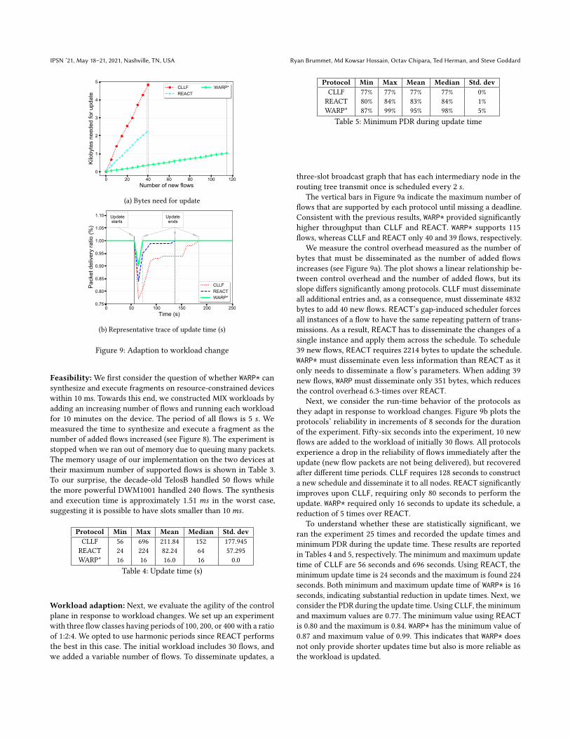
IPSN ’21, May 18–21, 2021, Nashville, TN, USA Ryan Brummet, Md Kowsar Hossain, Octav Chipara, Ted Herman, and Steve Goddard
0 20 40 60 80 100 120Number of new flows
0
1
2
3
4
5
Kilo
byte
s ne
eded
for u
pdat
eCLLFREACT
WARP*
(a) Bytes need for update
0 50 100 150 200 250Time (s)
0.75
0.80
0.85
0.90
0.95
1.00
1.05
1.10
Pac
ket d
eliv
ery
ratio
(%)
Update ends
Update starts
CLLFREACTWARP*
(b) Representative trace of update time (s)
Figure 9: Adaption to workload change
Feasibility:We first consider the question of whether WARP* cansynthesize and execute fragments on resource-constrained devices
within 10 ms. Towards this end, we constructed MIX workloads by
adding an increasing number of flows and running each workload
for 10 minutes on the device. The period of all flows is 5 𝑠 . We
measured the time to synthesize and execute a fragment as thenumber of added flows increased (see Figure 8). The experiment is
stopped when we ran out of memory due to queuing many packets.
The memory usage of our implementation on the two devices at
their maximum number of supported flows is shown in Table 3.
To our surprise, the decade-old TelosB handled 50 flows while
the more powerful DWM1001 handled 240 flows. The synthesis
and execution time is approximately 1.51 𝑚𝑠 in the worst case,
suggesting it is possible to have slots smaller than 10𝑚𝑠 .
Protocol Min Max Mean Median Std. devCLLF 56 696 211.84 152 177.945
REACT 24 224 82.24 64 57.295
WARP* 16 16 16.0 16 0.0
Table 4: Update time (s)
Workload adaption: Next, we evaluate the agility of the control
plane in response to workload changes. We set up an experiment
with three flow classes having periods of 100, 200, or 400 with a ratio
of 1:2:4. We opted to use harmonic periods since REACT performs
the best in this case. The initial workload includes 30 flows, and
we added a variable number of flows. To disseminate updates, a
Protocol Min Max Mean Median Std. devCLLF 77% 77% 77% 77% 0%
REACT 80% 84% 83% 84% 1%
WARP* 87% 99% 95% 98% 5%
Table 5: Minimum PDR during update time
three-slot broadcast graph that has each intermediary node in the
routing tree transmit once is scheduled every 2 𝑠 .
The vertical bars in Figure 9a indicate the maximum number of
flows that are supported by each protocol until missing a deadline.
Consistent with the previous results, WARP* provided significantly
higher throughput than CLLF and REACT. WARP* supports 115
flows, whereas CLLF and REACT only 40 and 39 flows, respectively.
We measure the control overhead measured as the number of
bytes that must be disseminated as the number of added flows
increases (see Figure 9a). The plot shows a linear relationship be-
tween control overhead and the number of added flows, but its
slope differs significantly among protocols. CLLF must disseminate
all additional entries and, as a consequence, must disseminate 4832
bytes to add 40 new flows. REACT’s gap-induced scheduler forces
all instances of a flow to have the same repeating pattern of trans-
missions. As a result, REACT has to disseminate the changes of a
single instance and apply them across the schedule. To schedule
39 new flows, REACT requires 2214 bytes to update the schedule.
WARP* must disseminate even less information than REACT as it
only needs to disseminate a flow’s parameters. When adding 39
new flows, WARP must disseminate only 351 bytes, which reduces
the control overhead 6.3-times over REACT.Next, we consider the run-time behavior of the protocols as
they adapt in response to workload changes. Figure 9b plots the
protocols’ reliability in increments of 8 seconds for the duration
of the experiment. Fifty-six seconds into the experiment, 10 new
flows are added to the workload of initially 30 flows. All protocols
experience a drop in the reliability of flows immediately after the
update (new flow packets are not being delivered), but recovered
after different time periods. CLLF requires 128 seconds to constructa new schedule and disseminate it to all nodes. REACT significantly
improves upon CLLF, requiring only 80 seconds to perform the
update. WARP* required only 16 seconds to update its schedule, a
reduction of 5 times over REACT.To understand whether these are statistically significant, we
ran the experiment 25 times and recorded the update times and
minimum PDR during the update time. These results are reported
in Tables 4 and 5, respectively. The minimum and maximum update
time of CLLF are 56 seconds and 696 seconds. Using REACT, theminimum update time is 24 seconds and the maximum is found 224
seconds. Both minimum and maximum update time of WARP* is 16
seconds, indicating substantial reduction in update times. Next, we
consider the PDR during the update time. UsingCLLF, the minimum
and maximum values are 0.77. The minimum value using REACTis 0.80 and the maximum is 0.84. WARP* has the minimum value of
0.87 and maximum value of 0.99. This indicates that WARP* does
not only provide shorter updates time but also is more reliable as
the workload is updated.
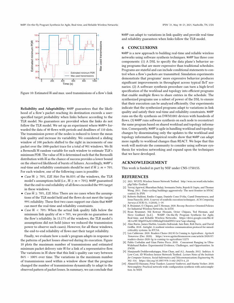
WARP: On-the-fly Program Synthesis for Agile, Real-time, and Reliable Wireless Networks IPSN ’21, May 18–21, 2021, Nashville, TN, USA
0 200 400 600 800 1000Time (s)
86
88
90
92
94
96
98
100E
stim
ated
min
imum
PD
R
0
1
2
3
Max
use
d tra
nsm
issi
ons
Estimated minimum PDRMax used transmissions
Figure 10: Estimated𝑚 and max. used transmissions of a flow’s link
Reliability and Adaptability: WARP guarantees that the likeli-
hood of a flow’s packet reaching its destination exceeds a user-
specified target probability when links behave according to the
TLR model. No guarantees are provided when the links do not
follow the TLR model. We set up an experiment where WARP* for-warded the data of 40 flows with periods and deadlines of 110 slots.
The transmission power of the nodes is reduced to lower the mean
link quality and increase its variability. We considered a sliding
window of 100 packets shifted to the right in increments of one
packet over the 1000-packet trace for a total of 901 windows. We fit
a Bernoulli𝑚 random variable for each window to estimate TLR’s
minimum PDR. The value of𝑚 is determined such that the Bernoulli
distribution with𝑚 as the chance of success provides a lower bound
on the observed likelihood of bursts of failures. Accordingly, WARP’sreal-time and reliability constraints should be met if𝑚 ≥ 𝑚 = 70%.
For each window, one of the following cases is possible:
• Case 𝑚 ≥ 70%, E2E Met: For 86.83% of the windows, the TLR
model’s assumptions held (i.e.,𝑚 ≥ 𝑚 = 70%). WARP guaranteed
that the end-to-end reliability of all flows exceeded the 99% target
in these windows.
• Case𝑚 ≥ 70%, E2E Miss: There are no cases when the assump-
tions of the TLR model held and the flows do not meet the target
99% reliability. These first two cases support our claim that WARPcan meet the real-time and reliability constraints.
• Case 𝑚 < 70%: When the actual link quality falls below the
minimum link quality of𝑚 = 70%, we provide no guarantees on
the flow’s reliability. In 13.17% of the windows, the TLR model’s
assumptions did not hold (since we reduced the transmission
power to observe such cases). However, for all these windows,
the end-to-end reliability of flows met their target reliability.
Finally, we evaluate how a node’s program adapts in response to
the patterns of packet losses observed during its execution. Figure
10 plots the maximum number of transmissions and estimated
minimum packet delivery rate𝑚 for a link of a representative flow.
The variations in𝑚 show that this link’s quality can vary between
86% – 100% over time. The variations in the maximum number
of transmissions used within a window show that the program
changed the number of transmissions dynamically to adapt to the
observed pattern of packet losses. In summary, we can conclude that
WARP can adapt to variations in link quality and provide real-time
and reliability guarantees when links follow the TLR model.
6 CONCLUSIONSWARP is a new approach to building real-time and reliable wireless
networks using software synthesis techniques. WARP has three core
components: (1) A DSL to specify the data plane’s behavior us-
ing programs that are more expressive than traditional schedules.
Programs are stateful and can include conditional statements to con-
trol when a flow’s packets are transmitted. Simulation experiments
demonstrate that programs’ more expressive behavior produces
significant improvements in throughput across typical IIoT sce-
narios. (2) A software synthesis procedure can turn a high-level
specification of the workload and topology into efficient programs
that enable multiple flows to share entries in the schedule. The
synthesized programs use a subset of power of the DSL to ensure
that their execution can be analyzed efficiently. Our experiments
indicate that the synthesized programs adapt to variations in link
quality and satisfy their real-time and reliability constraints. WARPruns on-the-fly synthesis on DWM1001 devices with hundreds of
flows. (3) WARP runs software synthesis on each node to reconstruct
the same program based on shared workload and topology informa-
tion. Consequently, WARP is agile in handlingworkload and topologychanges by disseminating only the updates to the workload and
topology information. Empirical results show that WARP can adapt
more rapidly to workload changes than REACT. We hope that this
work will motivate the community to consider using software syn-
thesis for wireless networking and expand upon the techniques
that we have developed.
ACKNOWLEDGEMENTThis work is funded in part by NSF under CNS-1750155.
REFERENCES[1] 2021. WUSTLWireless Sensor Network Testbed. http://wsn.cse.wustl.edu/index.
php?title=Testbed
[2] Yuvraj Agarwal, Bharathan Balaji, Seemanta Dutta, Rajesh K Gupta, and Thomas
Weng. 2011. Duty-cycling buildings aggressively: The next frontier in HVAC
control. In IPSN.[3] Roberto Baldoni, Emilio Coppa, Daniele Cono D’elia, Camil Demetrescu, and
Irene Finocchi. 2018. A survey of symbolic execution techniques. ACMComputingSurveys (CSUR) 51, 3 (2018), 1–39.
[4] R. Brummet, O. Chipara, and T. Herman. 2020. Recorp: Receiver-Oriented Policies
for Industrial Wireless Networks. In IoTDI.[5] Ryan Brummet, Md Kowsar Hossain, Octav Chipara, Ted Herman, and
Steve Goddard. [n.d.]. WARP: On-the-fly Program Synthesis for Agile,
Real-time, and Reliable Wireless Networks. https://drive.google.com/file/d/
1K1ve9fC3Hp0VOaAUvH0bxhgD2sIuEFH3/view?usp=sharing.
[6] Alan Burns, James Harbin, Leandro Indrusiak, Iain Bate, Rob Davis, and David
Griffin. 2018. Airtight: A resilient wireless communication protocol for mixed-
criticality systems. In RTCSA.[7] Len Calderone. 2020. Readers Choice 202:5G Is Coming to Agriculture. Agritech
Tomorrow (Dec 2020). https://www.agritechtomorrow.com/article/2020/07/
readers-choice-2020-5g-is-coming-to-agriculture/12275
[8] Pablo Corbalán and Gian Pietro Picco. 2018. Concurrent Ranging in Ultra-
Wideband Radios: Experimental Evidence, Challenges, and Opportunities. In
EWSN.[9] Manjunath Doddavenkatappa, Mun Chan, and A.L. Ananda. 2012. Indriya: A
Low-Cost, 3D Wireless Sensor Network Testbed. Lecture Notes of the Institutefor Computer Sciences, Social-Informatics and Telecommunications Engineering 90,
302–316. https://doi.org/10.1007/978-3-642-29273-6_23
[10] Ahmed El-Hassany, Petar Tsankov, Laurent Vanbever, and Martin Vechev. 2018.
Netcomplete: Practical network-wide configuration synthesis with autocomple-
tion. In NSDI.
IPSN ’21, May 18–21, 2021, Nashville, TN, USA Ryan Brummet, Md Kowsar Hossain, Octav Chipara, Ted Herman, and Steve Goddard
[11] Atis Elsts, Seohyang Kim, Hyung-Sin Kim, and Chongkwon Kim. 2020. An
empirical survey of autonomous scheduling methods for TSCH. IEEE Access(2020).
[12] Federico Ferrari, Marco Zimmerling, Luca Mottola, and Lothar Thiele. 2012.
Low-Power Wireless Bus. In SenSys.[13] Karen Field. 2020. Embracing IoT tech, John Deere plows a path
to autonomous machines. Fierce Electronics (Nov 2020). https:
//www.fierceelectronics.com/sensors/embracing-iot-tech-john-deere-plows-a-
path-to-autonomous-machines
[14] A. Gonga, O. Landsiedel, P. Soldati, and M. Johansson. 2012. Revisiting Multi-
channel Communication to Mitigate Interference and Link Dynamics in Wireless
Sensor Networks. In ICDCS.[15] Dolvara Gunatilaka and Chenyang Lu. 2020. REACT: an Agile Control Plane for
Industrial Wireless Sensor-Actuator Networks. In IoTDI.[16] James Harbin, Alan Burns, Robert I Davis, Leandro Soares Indrusiak, Iain Bate,
and David Griffin. 2019. The AirTight Protocol for Mixed Criticality Wireless
CPS. TCPS (2019).[17] OzlemDurmaz Incel. 2011. A survey onmulti-channel communication in wireless
sensor networks. Computer Networks (2011).[18] Chenyang Lu, Abusayeed Saifullah, Bo Li, Mo Sha, Humberto Gonzalez, Dolvara
Gunatilaka, Chengjie Wu, Lanshun Nie, and Yixin Chen. 2015. Real-time wireless
sensor-actuator networks for industrial cyber-physical systems. Proc. IEEE (2015).[19] Emerson Process management. 2016. System Engineering Guidelines IEC 62591
WirelessHART.
[20] Venkata Prashant Modekurthy, Abusayeed Saifullah, and Sanjay Madria. 2019.
DistributedHART: A distributed real-time scheduling system for wirelesshart
networks. In RTAS.[21] Marcelo Nobre, Ivanovitch Silva, and Luiz Affonso Guedes. 2015. Routing and
scheduling algorithms for WirelessHART Networks: a survey. Sensors (2015).[22] Pangun Park, Sinem Coleri Ergen, Carlo Fischione, Chenyang Lu, and Karl Henrik
Johansson. 2017. Wireless network design for control systems: A survey. IEEECommunications Surveys & Tutorials (2017).
[23] Abusayeed Saifullah, You Xu, and Chenyang Lu. 2010. Real-Time Scheduling for
WirelessHART Networks. In RTSS.[24] Tianyu Zhang, Tao Gong, Zelin Yun, Song Han, Qingxu Deng, and Xiaobo Sharon
Hu. 2018. FD-PaS: A fully distributed packet scheduling framework for handling
disturbances in real-time wireless networks. In RTAS.[25] Marco Zimmerlinonga, Luca Mottola, Pratyush Kumar, Federico Ferrari, and
Lothar Thiele. 2017. Adaptive real-time communication for wireless cyber-
physical systems. TCPS (2017).
Related Documents