Turk J Elec Eng & Comp Sci (2016) 24: 849 – 862 c ⃝ T ¨ UB ˙ ITAK doi:10.3906/elk-1305-110 Turkish Journal of Electrical Engineering & Computer Sciences http://journals.tubitak.gov.tr/elektrik/ Research Article Walsh series modeling and estimation in sensorless position control of electrical drives Hamidreza SHIRAZI, Jalal NAZARZADEH * Department of Electrical Engineering, Faculty of Engineering, Shahed University, Tehran, Iran Received: 17.05.2013 • Accepted/Published Online: 02.12.2013 • Final Version: 23.03.2016 Abstract: High-performance electrical drives can be achieved by using field-oriented controllers, which make torque and flux naturally decoupled. A conventional vector-controlled drive has the disadvantage of either requiring flux and speed sensors or being affected by rotor resistance, which varies along with the motor performance. The presented paper focuses on developing a high-performance sensorless rotor flux-oriented controller of an induction machine independent of the rotor resistance variation. This method applies spectral theory of Walsh functions, which are one of the most helpful members of piecewise constant basis functions in solving dynamic models. Inherent characteristics of Walsh functions and application of an operational matrix will make the system handy and robust against inverter switching effects. Key words: Induction machine, vector control, parameter estimation, position control, sensorless control, spectral analysis, Walsh series 1. Introduction Decoupling control of electromagnetic torque and flux is a desirable achievement in advanced control drives of induction machines. The amplitude and the position of the rotor flux phasor are two important variables that have to be simultaneously observed in rotor flux-oriented control (RFOC) [1]. Since the rotor flux vector varies, a high-performance electrical drive should consist of an online rotor flux observer and rotor speed estimators. As air gap flux in induction machines includes several phasor space harmonics, shaft-mounted sensors in direct control of RFOC drives have lower reliability along with extra expenses. Hence, sensorless vector control has been getting more attention among researchers as a mature technology. Several field-oriented induction motor drive methods without rotational transducers have been proposed [2]. In [3], the authors proposed a fuzzy controller, which was applied in direct torque neuro-fuzzy control of an induction motor, taking advantage of a time-variant PI controller. The disadvantage of these methods is that the rotor resistance variation causes an error in rotor flux observation and they need the motor speed sensor [4]. Different approaches to rotor resistance estimation have been analyzed in some papers. Some methods analyze estimation of rotor resistance based on model reference adaptive systems. In these methods, an error signal detects variation effects of the time constant in a rotor circuit, which can be realized by using a rotor flux computer [4] or torque signal [5]. This method is very sensitive to motor parameters’ variation, which results in low performance [6]. On the other hand, the process of estimation can be done by sampling input and output signals. Using sliding mode control [7] and Kalman filters [8] in the estimation process are some examples to be * Correspondence: [email protected] 849

Welcome message from author
This document is posted to help you gain knowledge. Please leave a comment to let me know what you think about it! Share it to your friends and learn new things together.
Transcript
Turk J Elec Eng & Comp Sci
(2016) 24: 849 – 862
c⃝ TUBITAK
doi:10.3906/elk-1305-110
Turkish Journal of Electrical Engineering & Computer Sciences
http :// journa l s . tub i tak .gov . t r/e lektr ik/
Research Article
Walsh series modeling and estimation in sensorless position control of electrical
drives
Hamidreza SHIRAZI, Jalal NAZARZADEH∗
Department of Electrical Engineering, Faculty of Engineering, Shahed University, Tehran, Iran
Received: 17.05.2013 • Accepted/Published Online: 02.12.2013 • Final Version: 23.03.2016
Abstract: High-performance electrical drives can be achieved by using field-oriented controllers, which make torque
and flux naturally decoupled. A conventional vector-controlled drive has the disadvantage of either requiring flux and
speed sensors or being affected by rotor resistance, which varies along with the motor performance. The presented paper
focuses on developing a high-performance sensorless rotor flux-oriented controller of an induction machine independent of
the rotor resistance variation. This method applies spectral theory of Walsh functions, which are one of the most helpful
members of piecewise constant basis functions in solving dynamic models. Inherent characteristics of Walsh functions
and application of an operational matrix will make the system handy and robust against inverter switching effects.
Key words: Induction machine, vector control, parameter estimation, position control, sensorless control, spectral
analysis, Walsh series
1. Introduction
Decoupling control of electromagnetic torque and flux is a desirable achievement in advanced control drives of
induction machines. The amplitude and the position of the rotor flux phasor are two important variables that
have to be simultaneously observed in rotor flux-oriented control (RFOC) [1]. Since the rotor flux vector varies,
a high-performance electrical drive should consist of an online rotor flux observer and rotor speed estimators.
As air gap flux in induction machines includes several phasor space harmonics, shaft-mounted sensors in direct
control of RFOC drives have lower reliability along with extra expenses. Hence, sensorless vector control has
been getting more attention among researchers as a mature technology.
Several field-oriented induction motor drive methods without rotational transducers have been proposed
[2]. In [3], the authors proposed a fuzzy controller, which was applied in direct torque neuro-fuzzy control of an
induction motor, taking advantage of a time-variant PI controller. The disadvantage of these methods is that
the rotor resistance variation causes an error in rotor flux observation and they need the motor speed sensor [4].
Different approaches to rotor resistance estimation have been analyzed in some papers. Some methods
analyze estimation of rotor resistance based on model reference adaptive systems. In these methods, an error
signal detects variation effects of the time constant in a rotor circuit, which can be realized by using a rotor flux
computer [4] or torque signal [5]. This method is very sensitive to motor parameters’ variation, which results in
low performance [6]. On the other hand, the process of estimation can be done by sampling input and output
signals. Using sliding mode control [7] and Kalman filters [8] in the estimation process are some examples to be
∗Correspondence: [email protected]
849
SHIRAZI and NAZARZADEH/Turk J Elec Eng & Comp Sci
named. Because of noisy signals in the systems, these methods are unreliable and they also lose performance if
used for nonlinear models of the systems.
Different works have evaluated methods of rotor speed estimation. In [9,10], the MRAS method was
applied to estimate the rotor speed. Moreover, the rotor speed in an induction machine drive was given as
an unknown constant value and an extended Kalman filter was applied in the estimation process [11,12]. The
authors of [13] applied the least square method to find out the estimated value of the rotor speed where the
best fits interpolated measured signals of an induction machine with dynamic equations.
On the other hand, Walsh functions can be applied in order to study differential equations and dynamic
systems efficiently [14,15]. Walsh functions are one of the piecewise constant basis functions [16], which
can be applied in problem solving, e.g., optimization control, parameter identification, image processing,
communication, and harmonic elimination [17–19]. Walsh functions simplify the solution of nonlinear equations
while their piecewise properties decrease noise effects in the ultimate answer. In order to simplify and speed up
the solving process, an operational matrix can be used [20].
This paper presents a new online vector control scheme for induction motors that observes the rotor
flux orientation directly from machine equations without the need for rotor resistance knowledge. This method
applies stator current and voltage as input signals and thereafter estimates motor speed and observes the rotor
flux orientation. This process takes place in the Walsh domain with the help of operational matrices, since the
motor is analyzed at high speed in time intervals instead of taking samples. Individual characteristics of the
applied method diminish noise effects. In the end, as a pseudoinverse method is applied, the response gets more
reliable and precise.
2. Vector control in induction machines
In order to apply the system under control based on identifying needed parameters, the first essential step is
to have a simple and proper model of each involved component. In this section, an appropriate model for an
induction machine in different reference frames is defined.
3. Model of induction machines in arbitrary reference frame
This subsection elaborates the model of an induction machine in an arbitrary reference frame that rotates
at angular speed of ωe(α − β frame). In this arbitrary reference frame (Figure 1), the direct and quadratic
components of the stator and the rotor voltage equations of an induction machine can be stated as follows [1].
vsα = Rsisα + ψsα − ωeψsβ
vsβ = Rsisβ + ψsβ + ωeψsα(1)
0 = Rrirα + ψrα − (ωe − ωr)ψrβ
0 = Rrirα + ψrβ + (ωe − ωr)ψrα(2)
Here, vsα andvsβ are real and imaginary components of the stator voltage, and irα ,irβ ,isα , and isβ are
two components of the rotor and stator currents, respectively. These components are shown in Figure 1. In
Eq. (2), Rr and Rs are respectively the resistance for the rotor and stator and ψrα , ψrβ , ψsα , and ψsβ are
respectively two components of the rotor and stator fluxes, which can be determined as follows.
850
SHIRAZI and NAZARZADEH/Turk J Elec Eng & Comp Sci
+
+
+
–
–
–
asv
ibr
icrvbs
v cs
y Axis
ρ
ωr
si
ri
ψrψr Axis(x)ωψr
s ri
iar
isy isx
ωe
θr
θ
sgi
'
ri r ri
irx
iry
q Axis
Axisβ
Arbitrary Axis (α)
rqi
rdi
ri
si
ri
si
sqi
sdi
( )Stationary Axis d
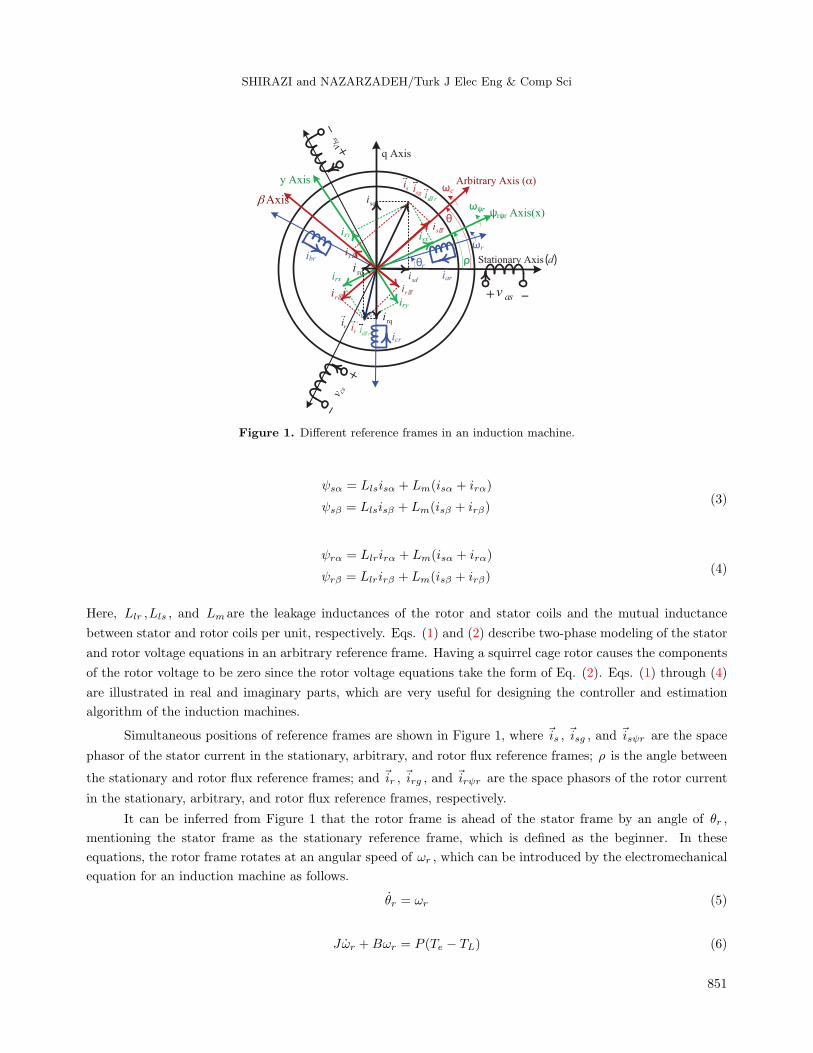
Figure 1. Different reference frames in an induction machine.
ψsα = Llsisα + Lm(isα + irα)
ψsβ = Llsisβ + Lm(isβ + irβ)(3)
ψrα = Llrirα + Lm(isα + irα)
ψrβ = Llrirβ + Lm(isβ + irβ)(4)
Here, Llr ,Lls , and Lm are the leakage inductances of the rotor and stator coils and the mutual inductance
between stator and rotor coils per unit, respectively. Eqs. (1) and (2) describe two-phase modeling of the stator
and rotor voltage equations in an arbitrary reference frame. Having a squirrel cage rotor causes the components
of the rotor voltage to be zero since the rotor voltage equations take the form of Eq. (2). Eqs. (1) through (4)
are illustrated in real and imaginary parts, which are very useful for designing the controller and estimation
algorithm of the induction machines.
Simultaneous positions of reference frames are shown in Figure 1, where is , isg , and isψr are the space
phasor of the stator current in the stationary, arbitrary, and rotor flux reference frames; ρ is the angle between
the stationary and rotor flux reference frames; and ir , irg , and irψr are the space phasors of the rotor current
in the stationary, arbitrary, and rotor flux reference frames, respectively.
It can be inferred from Figure 1 that the rotor frame is ahead of the stator frame by an angle of θr ,
mentioning the stator frame as the stationary reference frame, which is defined as the beginner. In these
equations, the rotor frame rotates at an angular speed of ωr , which can be introduced by the electromechanical
equation for an induction machine as follows.
θr = ωr (5)
Jωr +Bωr = P (Te − TL) (6)
851
SHIRAZI and NAZARZADEH/Turk J Elec Eng & Comp Sci
Here, P and Tl are the number of paired poles and load torque, and Te is the electromagnetic torque in an
induction machine, which can be determined as follows.
Te = 3P2 Lm (irαisβ − isαirβ)
= 3P2Lm
Lrψrg × isg
(7)
Here, ψrg is the vector of the rotor flux in the arbitrary reference frame.
4. Rotor flux-oriented control
The vector form of the variables can be substituted into Eq. (2) to determine a space phasor of the rotor voltage
relation of an induction machine as follows.
0 = Rrirψr +˙ψrψr + j (ωψr − ωr) ψrψr (8)
Here, ψrψr is the space phasor of the rotor flux in the rotor-flux reference frame. Combining Eqs. (3) and (4),
the space phasor of the rotor flux in the rotor flux reference frame can be obtained by the following.
ψrψr = Llrirψr + Lm(isψr + irψr) (9)
Because the rotor flux reference frame is aligned with rotor flux, ψr is real and we can write the following.
ψrψr =∣∣∣ψrψr∣∣∣ = ψrψr (10)
By combining Eqs. (8) and (9) to (10) and resolving the result into real and imaginary components, the modulus
and angular speed of the rotor flux space phasor can be obtained as follows.
Trψrψr + ψrψr = Lmisx (11)
ωψr = ωr +LmisyTrψrψr
(12)
Here, Tr is the time constant of the rotor circuit, which is as follows.
Tr =LrRr
(13)
The simultaneous position of the rotor flux (ρ) can be determined by using the angular speed of the rotor flux
(ωψr) in Eq. (12) as follows.
ρ = ωψr (14)
Mentioning Eq. (11), the recommended signal for the direct component of the stator current ( isx) in the steady
state can be calculated from the following.
isx =ψrcLm
(15)
852

SHIRAZI and NAZARZADEH/Turk J Elec Eng & Comp Sci
Here, ψrc is the out signal of the flux controller. The quadratic component of the stator current (isy) for
producing torque reference (Tref ) in the rotor flux frame can be obtained from Eq. (7) as follows.
isy =2
3P
LrTrefLmψrψr
(16)
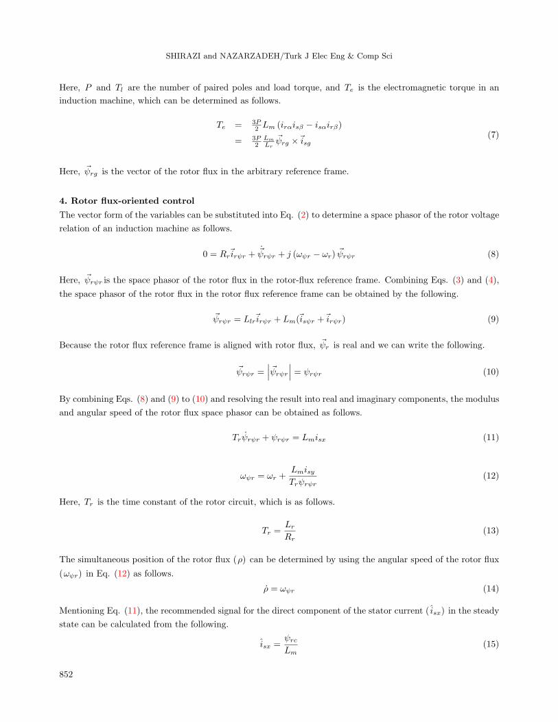
As Figure 2 shows, the rotor flux-oriented control can be performed by applying Eqs. (15) and (16).
Figure 2. Rotor flux-oriented control of an induction machine.
5. Rotor flux observation and speed estimation
Here the observation and estimation processes will be investigated in the stator reference frame (d− q) where
ωe in Eq. (1) will be substituted with zero. First the manner of calculating components of the rotor flux vector
using the stator and rotor components will be studied; applying produced components, this method estimates
the unknown rotor speed. Using each two components of Eq. (1) and then integrating them, we will have the
following.
ψsd =
∫t
lim0
(vsd −Rsisd) dt+ ψsd(0) (17)
ψsq =
∫t
lim0
(vsq −Rsisq) dt+ ψsq(0) (18)
Here, ψsd(0) and ψsq(0) are two initial values of the stator flux in the stationary reference frame. Real
components of the stator and rotor fluxes (ψsd and ψsq) can be determined by the following.
ψsd = Llsisd + Lm(isd + ird) (19)
ψrd = Llrird + Lm(isd + ird) (20)
By eliminating ird in Eqs. (19) and (20), we have the following.
ψsd = L′
sisd − ψrd (21)
853
SHIRAZI and NAZARZADEH/Turk J Elec Eng & Comp Sci
Here, L′
s is the transient inductance of the induction machine, which can be obtained by the following.
L′s = Lls +
LlrLmLlr + Lm
(22)
By substituting Eq. (21) into Eq. (17), we can get the following.
ψrd =
∫t
lim0
(vsd −Rsisd) dt+ ψsd(0)− L′sisd (23)
Similarly, by eliminating irq from the relations between imaginary components of the stator and rotor fluxes
(ψsq and ψrq) and substituting results into Eq. (18), we can write the following.
ψrq =
∫t
lim0
(vsq −Rsisq) dt+ ψsq(0)− L′sisq (24)
Based on Eqs. (23) and (24), we can estimate the real and imaginary components of the rotor flux vector in
the stationary reference frame ( ψrd and ψrq). Thus, regarding Figure 1, the quantity and position of the rotor
flux in the stationary reference frame can be obtained from the following.
ψrψr =√ψ2rd + ψ2
rq (25)
ρ = tan−1
(ψrdψrq
)(26)
Eqs. (25) and (26) make the rotor flux vector a known value that can be used in order to compute the rotor
speed and position. Moreover, the simultaneous values of the rotor resistance and rotor speed can be estimated
by stator currents and voltages in the stationary reference frame. Therefore, by substituting ird from Eq. (20)
into the real component of Eq. (2) in the stationary reference frame, we can conclude the following.
Rr
∫t
lim0
(LmLr
isd −1
Lrψrd
)dt− ωr
∫t
lim0ψrqdt = ψrd − ψrdi (27)
Similarly, by eliminating irq from the imaginary component in Eq. (2) in the stationary reference frame, we
have the following.
Rr
∫t
lim0
(LmLr
isq −1
Lrψrq
)dt+ ωr
∫t
lim0ψrddt = ψrq − ψrqi (28)
The last presented equation can be restated in matrix form as:[H11 H12
H21 H12
][Rr
ωr
]=
[U1
U2
], (29)
in which we have the following.
H11 =∫limt
0
(Lm
Lrisd − 1
Lrψrd
)dtH12 = −
∫limt
0 ψrqdt
H21 =∫limt
0
(Lm
Lrisq − 1
Lrψrq
)dtH22 =
∫limt
0 ψrddt
U1 = ψrd − ψrdiU2 = ψrq − ψrqi
(30)
854
SHIRAZI and NAZARZADEH/Turk J Elec Eng & Comp Sci
In order to produce the optimal estimation out of Eq. (29), this paper applies the least square method [21],
which minimizes the estimation process error. As can be seen, the least square estimation values for Rr and
ωr can be obtained from the following.
Rr
ωr
=
[ H11 H12
H21 H22
]T [H11 H12
H21 H22
]−1 [H11 H12
H21 H22
]T [U1
U2
](31)
Getting to estimation values from Eq. (31) requires us to solve integral equations; here we apply the Walsh
series to find algebraic relations for the estimation of rotor resistance and speed.
6. Estimating rotor resistance and speed by Walsh series
In this section, the properties in the Appendix will be applied in order to solve the dynamic equations used
in Eqs. (23), (24), and (31). As a result, the rotor speed and the rotor resistance values will be estimated
taking advantage of the Walsh series. First, assuming that the voltage and current of the stator are known
signals, transformation of the signals to the Walsh domain takes advantage of Eqs. (A.2), (A.3), and (A.4).
According to Eq. (A.3), it is necessary to get an integral of the signal over t ∈ [ts, tf ) in order to define its
Walsh coefficient in Eq. (A.4), where ts stands for the start time of each process interval and tf shows the end
of them. Based on the order of the Walsh series, each process interval can be divided into n subintervals. In
order to find the arrays of Eq. (A.4) the integral of the signal in each subinterval will be computed. Thereafter,
arrays attributed to each Walsh function can be obtained from the sum of all quantities, where the quantity will
be negative or positive based on the sign of that function in the mentioned subinterval. Finally, the definition
of real and imaginary components of signals with the Walsh series will be as follows.
vsd = cTvsdw(t) vsq = cTvsqw(t) (32)
isd = cTisdw(t) isq = cTisqw(t) (33)
Using the operational matrix in Eq. (A.8) and combining Eqs. (32) and (33) with Eqs. (23) and (24), the
Walsh coefficient vectors’ real and imaginary components of the stator flux can be obtained as follows.
cψsd = ET (cvsd −Rscisd) + cψsd0 (34)
cψsq = ET (cvsq −Rscisq) + cψsq0 (35)
Here, cψsd and cψsq are Walsh coefficient vectors for two components of the stator flux, and cψsd0 and cψsq0
are constant initial values of the stator flux components, which are zero for the starting conditions. With Eqs.
(23), (24), (34), and (35), the Walsh coefficient vectors for the two components of the rotor flux can be obtained
as follows.
cψrd = ET (cvsd −Rscisd) + cψsd0 − L′scisd (36)
cψrq = ET (cvsq −Rscisq) + cψsq0 − L′scisq (37)
855
SHIRAZI and NAZARZADEH/Turk J Elec Eng & Comp Sci
These relations can be used for determination of direct and quadrature components of the rotor flux in the
stationary reference frame on t ∈ [ts, tf ). Thus, at t = t−f , we have the following.
ψrd(t−f ) = cT
ψrdw(t−f ) (38)
ψrq(t−f ) = cT
ψrqw(t−f ) (39)
Here, t−f means approaching tf from below. By substituting Eqs. (38) and (39) into Eqs. (25) and (26), the
amplitude and position of the rotor flux can be obtained as follows.
ψrψr =(cTψrd
w(t−f )wT (t−f )cψrd + cT
ψrqw(t−f )w
T (t−f )cψrq
) 12
(40)
ρ = tan−1
(cTψrd
w(t−f )
cTψrq
w(t−f )
)(41)
The initial value for the first time interval is zero. The initial value for each interval is the ultimate value forthe last interval. Thereafter, having the above variables in the Walsh domain, the optimal estimation in Eq.
(31) can be obtained as: Rr
ωr
=(HT H
)−1
HT u, (42)
in which we have the following.
H =1
Lr
ET(Lmcisd − cψrd
)−LrET cψrq
LrET cψrd ET
(Lmcisq − cψrq
) (43)
u =
[cψrd − cψrd0
cψrq − cψrq0
](44)
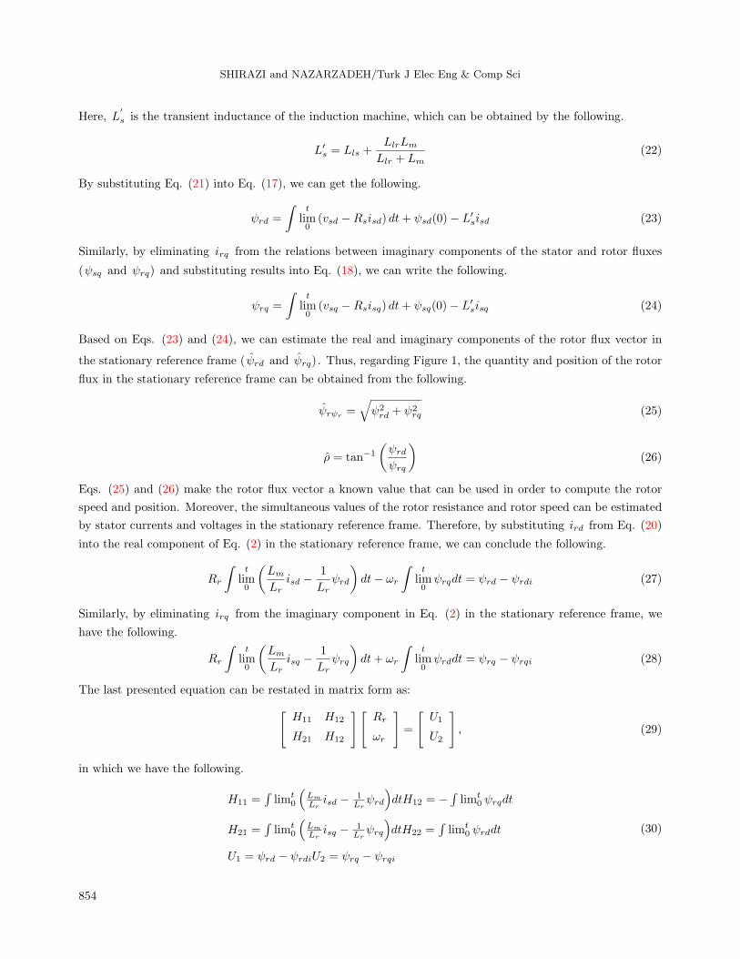
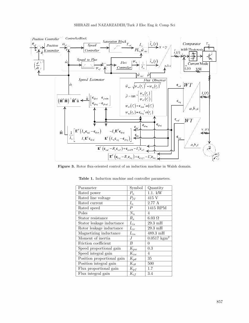
In this section, the estimation process was elaborated in the Walsh domain. Figure 3 shows the closed-loop
speed controlled for an induction machine where the rotor speed estimator is implemented from Eq. (42) by
Walsh functions. In order to have better insight about this process, the next section is allocated to a case study
on the estimation of the speed and resistance of the rotor.
7. Illustrative example
This section illustrates the estimation process on one time interval (∆t = 5 ms) and uses a 2-order Walsh
series (k = 2) in order to evaluate the method. In this section, the machine and controller parameters are as
introduced in Table 1.
856
SHIRAZI and NAZARZADEH/Turk J Elec Eng & Comp Sci
Figure 3. Rotor flux-oriented control of an induction machine in Walsh domain.
Table 1. Induction machine and controller parameters.
Parameter Symbol QuantityRated power Pn 1.1. kWRated line voltage PII 415 VRated current In 2.77 ARated speed P 1415 RPMPoles Nn 4Stator resistance Rs 6.03 ΩStator leakage inductance Lis 29.3 mHRotor leakage inductance Lir 29.3 mHMagnetizing inductance Lin 489.3 mHMoment of inertia J 0.0517 kgm2
Friction coefficient B 0Speed proportional gain Kpw 0.3Speed integral gain Kiw 4Position proportional gain Kpθ 35Position integral gain Kiθ 500Flux proportional gain Kpf 1.7Flux integral gain Kif 3.4
857
SHIRAZI and NAZARZADEH/Turk J Elec Eng & Comp Sci
Variation of the rotor resistance is given as follows.
Rr =
6.0850 t ≤ 0.1
4t+ 2.0850 0.1 ≤ t ≤ 0.2
8.5190 t ≥ 0.2
(45)
In this process, voltages and currents of the stator are known as input values. Hence, the Walsh coefficient
vectors of real and imaginary components of these signals are available. With this preface, the coefficient vectors
for each component of Eqs. (36) and (37) in milliwebers can be written as follows.
cψrd=
0.1cvsd0 − 61.0cisd0 + 0.1cvsd1 − 0.3cisd1 + 1059.9cψsd0
0
−0.1cvsd0 + 0.3cisd0 − 60.4cisd1
(46)
cψrq=
0.1cvsq0 − 61.0c
isq0 + 0.1c
vsq1 − 0.3c
isq1 + 1059.9c
ψsqi
0
−0.1cvsq0 + 0.3cisq0 − 60.4c
isq1
(47)
Substituting Eqs. (46) and (47) into Eqs. (43) and (44), we have the following.
0.9(cisd0 − cψrd
1 )− 1.9cψrd
0 + 0.4cisd1 −cψrq
0 − 0.5cψrq
1
−0.5cisd0 + cψrd
0 0.5cψrq
0
0.9(cisq0 − c
ψrq
1 )− 1.9cψrq
0 + 0.4cisq1 cψrd
0 + 0.5cψrd
1
−0.5cisq0 + c
ψrq
0 −0.5cψrd
0
Rr
ωr
= 104
cψrd
0 − cψrd0
0
cψrd
1
cψrq
0 − cψrq0
0
cψrq
1
(48)
For an evaluation of the estimation method, the matrix relation in Eq. (48) will be extracted in t = 0.1 s. In
this moment, the Walsh coefficients of the voltages and currents of the stator in the induction machine are as
follows.
cvsd =
[0
300
]cvsq =
[0
300
](49)
cisd =
[1.9786
0.0095
]cisq =
[1.5466
0.0135
](50)
Initial values for the direct and quadrature fluxes in the stationary reference frame are as follows.
cψrd0
0 = 0.86138 (51)
cψrq0
0 = 0.61284 (52)
858
SHIRAZI and NAZARZADEH/Turk J Elec Eng & Comp Sci
Thereafter, by applying Eq. (48) to (52), we have the following.−0.31291 0.570932
0.154233 −0.285547
−0.364699 −0.808202
0.179005 0.404087
Rr
ωr
=
1.104950
−0.566727
−6.478690
3.219450
(53)
With Eq. (42), the estimated values for the rotor resistance and speed can be determined as follows.
Rr = 6.0850Ω (54)
ωr = 5.2706 rad/σ (55)
Continuing this process, we can find similar results for Rr and ωr through time. Table 2 shows these estimated
values by different orders of Walsh functions.
Table 2. Estimated rotor resistance and speed by Walsh functions with different orders.
Time Rotor resistance Estimated rotor Rotor speed Estimated rotor
(s) Rr(Ω) Resistance Rr(Ω) ωr (rad/s) Speed ωr (rad/s)k = 2 k = 4 k = 2 k = 4 k = 2 k = 4
0.10 6.0850 6.0850 6.0850 5.0972 5.1115 5.2706 5.27630.12 6.5718 6.4478 6.4575 3.4820 3.4715 4.0230 4.03540.14 7.0586 6.9450 6.9374 1.2513 1.2482 1.8979 1.90570.16 7.5454 7.4252 7.4126 –0.9237 –0.9241 –0.4006 –0.38460.18 8.0322 7.9047 7.8949 –2.4916 –2.4914 –2.2088 –2.18820.20 8.5190 8.3948 8.3661 –3.1006 –3.1224 –3.2173 –3.2556
8. Simulation results
This section studies the system performance under different conditions. The machine used in these simulations
has parameters the same as those in Table 1. The reference value has been set as 0.1 rad for the desirable
position and 1 Wb has been taken as rated flux. For examining the efficiency of the system performance under
rotor resistance variation this value was set to 1.4 times its preliminary value. This increment started to take
part in 0.1 s with a ramp pattern of which the controller was completely unaware. In this study, the 4-order
Walsh series was applied and new estimated values were uploaded to controller in each 5 ms. By operating
the motor as seen in Figure 3, the controller started to estimate the rotor flux and took advantage of that in
order to estimate the rotor speed, which was used in estimation of the rotor position. These estimated values
helped the closed-loop controller in making the motor follow its references. Figure 4 shows the performance of
the system under unit and ramp changes of the reference value.
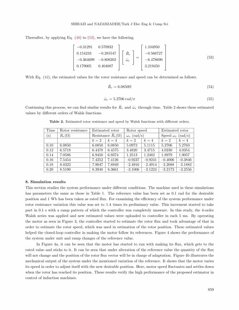
In Figure 4a, it can be seen that the motor has started to run with making its flux, which gets to the
rated value and sticks to it. It can be seen that under alteration of the reference value the quantity of the flux
will not change and the position of the rotor flux vector will be in charge of adaptation. Figure 4b illustrates the
mechanical output of the system under the mentioned variation of the reference. It shows that the motor varies
its speed in order to adjust itself with the new desirable position. Here, motor speed fluctuates and settles down
when the rotor has reached its position. These results verify the high performance of the proposed estimator in
control of induction machines.
859
SHIRAZI and NAZARZADEH/Turk J Elec Eng & Comp Sci
Figure 4. Closed-loop response of the sensorless vector control system with Walsh function estimator.
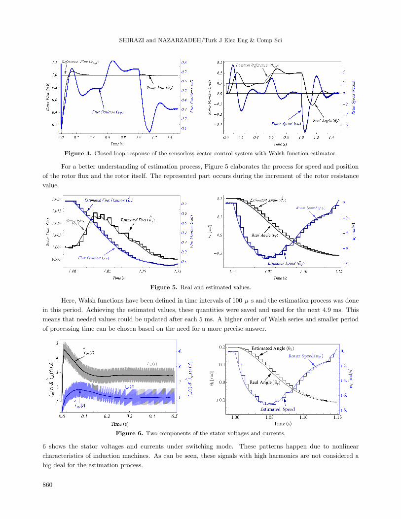
For a better understanding of estimation process, Figure 5 elaborates the process for speed and position
of the rotor flux and the rotor itself. The represented part occurs during the increment of the rotor resistance
value.
Figure 5. Real and estimated values.
Here, Walsh functions have been defined in time intervals of 100 µ s and the estimation process was done
in this period. Achieving the estimated values, these quantities were saved and used for the next 4.9 ms. This
means that needed values could be updated after each 5 ms. A higher order of Walsh series and smaller period
of processing time can be chosen based on the need for a more precise answer.
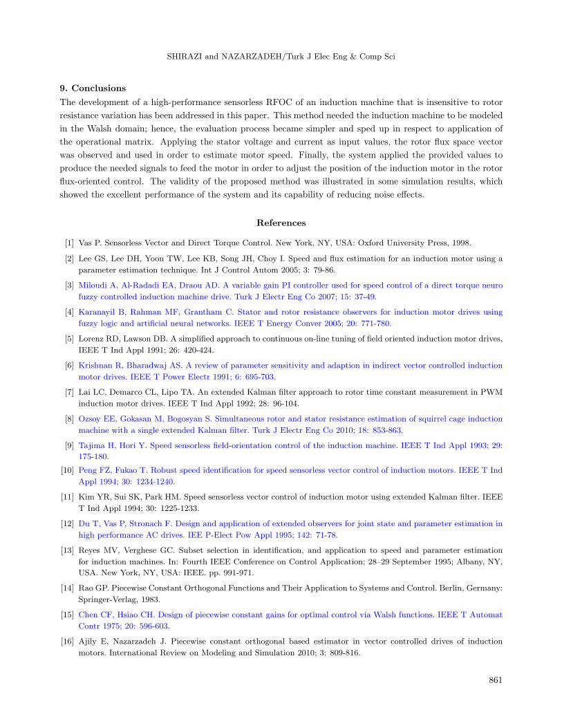
Figure 6. Two components of the stator voltages and currents.
6 shows the stator voltages and currents under switching mode. These patterns happen due to nonlinear
characteristics of induction machines. As can be seen, these signals with high harmonics are not considered a
big deal for the estimation process.
860
SHIRAZI and NAZARZADEH/Turk J Elec Eng & Comp Sci
9. Conclusions
The development of a high-performance sensorless RFOC of an induction machine that is insensitive to rotor
resistance variation has been addressed in this paper. This method needed the induction machine to be modeled
in the Walsh domain; hence, the evaluation process became simpler and sped up in respect to application of
the operational matrix. Applying the stator voltage and current as input values, the rotor flux space vector
was observed and used in order to estimate motor speed. Finally, the system applied the provided values to
produce the needed signals to feed the motor in order to adjust the position of the induction motor in the rotor
flux-oriented control. The validity of the proposed method was illustrated in some simulation results, which
showed the excellent performance of the system and its capability of reducing noise effects.
References
[1] Vas P. Sensorless Vector and Direct Torque Control. New York, NY, USA: Oxford University Press, 1998.
[2] Lee GS, Lee DH, Yoon TW, Lee KB, Song JH, Choy I. Speed and flux estimation for an induction motor using a
parameter estimation technique. Int J Control Autom 2005; 3: 79-86.
[3] Miloudi A, Al-Radadi EA, Draou AD. A variable gain PI controller used for speed control of a direct torque neuro
fuzzy controlled induction machine drive. Turk J Electr Eng Co 2007; 15: 37-49.
[4] Karanayil B, Rahman MF, Grantham C. Stator and rotor resistance observers for induction motor drives using
fuzzy logic and artificial neural networks. IEEE T Energy Conver 2005; 20: 771-780.
[5] Lorenz RD, Lawson DB. A simplified approach to continuous on-line tuning of field oriented induction motor drives,
IEEE T Ind Appl 1991; 26: 420-424.
[6] Krishnan R, Bharadwaj AS. A review of parameter sensitivity and adaption in indirect vector controlled induction
motor drives. IEEE T Power Electr 1991; 6: 695-703.
[7] Lai LC, Demarco CL, Lipo TA. An extended Kalman filter approach to rotor time constant measurement in PWM
induction motor drives. IEEE T Ind Appl 1992; 28: 96-104.
[8] Ozsoy EE, Gokasan M, Bogosyan S. Simultaneous rotor and stator resistance estimation of squirrel cage induction
machine with a single extended Kalman filter. Turk J Electr Eng Co 2010; 18: 853-863.
[9] Tajima H, Hori Y. Speed sensorless field-orientation control of the induction machine. IEEE T Ind Appl 1993; 29:
175-180.
[10] Peng FZ, Fukao T. Robust speed identification for speed sensorless vector control of induction motors. IEEE T Ind
Appl 1994; 30: 1234-1240.
[11] Kim YR, Sui SK, Park HM. Speed sensorless vector control of induction motor using extended Kalman filter. IEEE
T Ind Appl 1994; 30: 1225-1233.
[12] Du T, Vas P, Stronach F. Design and application of extended observers for joint state and parameter estimation in
high performance AC drives. IEE P-Elect Pow Appl 1995; 142: 71-78.
[13] Reyes MV, Verghese GC. Subset selection in identification, and application to speed and parameter estimation
for induction machines. In: Fourth IEEE Conference on Control Application; 28–29 September 1995; Albany, NY,
USA. New York, NY, USA: IEEE. pp. 991-971.
[14] Rao GP. Piecewise Constant Orthogonal Functions and Their Application to Systems and Control. Berlin, Germany:
Springer-Verlag, 1983.
[15] Chen CF, Hsiao CH. Design of piecewise constant gains for optimal control via Walsh functions. IEEE T Automat
Contr 1975; 20: 596-603.
[16] Ajily E, Nazarzadeh J. Piecewise constant orthogonal based estimator in vector controlled drives of induction
motors. International Review on Modeling and Simulation 2010; 3: 809-816.
861
SHIRAZI and NAZARZADEH/Turk J Elec Eng & Comp Sci
[17] Melgoza JR, Heydt GT, Keyhani A, Agrawal BL, Selin D. An algebraic approach for identifying operating point
dependent parameters of synchronous machines using orthogonal series expansions. IEEE T Energy Conver 1991;
16: 420-424.
[18] Lazaridis G, Petrou M. Image registration using the Walsh transform. IEEE T Image Process 2006; 15: 2343-2357.
[19] Windeatt T, Zor C. Minimising added classification error using Walsh coefficients. IEEE T Neural Networ 2011;
22: 334-1339.
[20] Radmanesh HR, Shakouri H, Nazarzadeh J. Synchronous generator parameter estimation using pseudo-inverse
method in hybrid domain. In: IEEE 2007 International Symposium on Industrial Electronics; 4–7 June 2007; Vigo,
Spain. New York, NY, USA: IEEE. pp. 335-340.
[21] Simon D. Optimal State Estimation, Kalman, H∞ , and Non-Linear Approaches. Hoboken, NJ, USA: Wiley, 2006.
[22] Razzaghi M, Nazarzadeh J. Walsh functions. Wiley Encyclopedia of Electrical and Electronic Engineering 1999; 23:
429-440.
862
SHIRAZI and NAZARZADEH/Turk J Elec Eng & Comp Sci
Appendix. Walsh series.
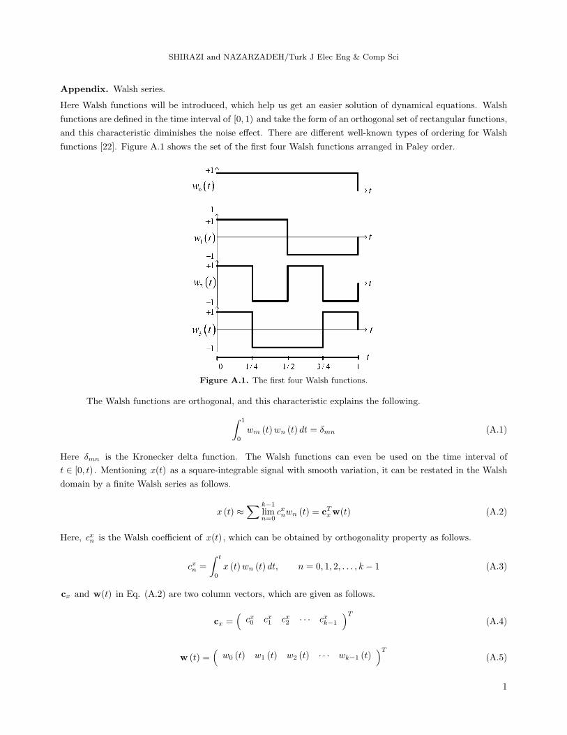
Here Walsh functions will be introduced, which help us get an easier solution of dynamical equations. Walsh
functions are defined in the time interval of [0, 1) and take the form of an orthogonal set of rectangular functions,
and this characteristic diminishes the noise effect. There are different well-known types of ordering for Walsh
functions [22]. Figure A.1 shows the set of the first four Walsh functions arranged in Paley order.
Figure A.1. The first four Walsh functions.
The Walsh functions are orthogonal, and this characteristic explains the following.∫ 1
0
wm (t)wn (t) dt = δmn (A.1)
Here δmn is the Kronecker delta function. The Walsh functions can even be used on the time interval of
t ∈ [0, t). Mentioning x(t) as a square-integrable signal with smooth variation, it can be restated in the Walsh
domain by a finite Walsh series as follows.
x (t) ≈∑ k−1
limn=0
cxnwn (t) = cTxw(t) (A.2)
Here, cxn is the Walsh coefficient of x(t), which can be obtained by orthogonality property as follows.
cxn =
∫ t
0
x (t)wn (t) dt, n = 0, 1, 2, . . . , k − 1 (A.3)
cx and w(t) in Eq. (A.2) are two column vectors, which are given as follows.
cx =(cx0 cx1 cx2 · · · cxk−1
)T(A.4)
w (t) =(w0 (t) w1 (t) w2 (t) · · · wk−1 (t)
)T(A.5)
1
SHIRAZI and NAZARZADEH/Turk J Elec Eng & Comp Sci
For square-integrable x(t) and y(t) on the time interval of t ∈ [0, t), cx and cy are their Walsh coefficient
vectors, respectively, and then we have the following.
x (t)± y (t) ≈ (cx ± cy)Tw(t) (A.6)
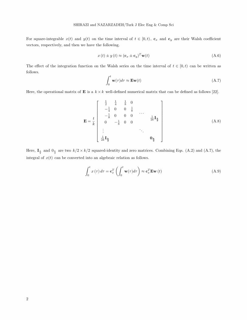
The effect of the integration function on the Walsh series on the time interval of t ∈ [0, t) can be written as
follows. ∫ t
0
w(τ)dτ ≈ Ew(t) (A.7)
Here, the operational matrix of E is a k× k well-defined numerical matrix that can be defined as follows [22].
E =t
k
12
14
18 0
−14 0 0 1
8
−18 0 0 0
0 − 18 0 0
· · ·
.... . .
12k I k
2
12k I k
20 k
2
(A.8)
Here, I k2and 0 k
2are two k/2× k/2 squared-identity and zero matrices. Combining Eqs. (A.2) and (A.7), the
integral of x(t) can be converted into an algebraic relation as follows.
∫ t
0
x (τ) dτ = cTx
(∫ t
0
w(τ)dτ
)≈ cTxEw (t) (A.9)
2
Related Documents