Wall-modeled large-eddy simulation of the flow past a rod ...

HAL Id: hal-02084828https://hal.archives-ouvertes.fr/hal-02084828

Submitted on 20 Apr 2019

HAL is a multi-disciplinary open accessarchive for the deposit and dissemination of sci-entific research documents, whether they are pub-lished or not. The documents may come fromteaching and research institutions in France orabroad, or from public or private research centers.

L’archive ouverte pluridisciplinaire HAL, estdestinée au dépôt et à la diffusion de documentsscientifiques de niveau recherche, publiés ou non,émanant des établissements d’enseignement et derecherche français ou étrangers, des laboratoirespublics ou privés.

Wall-modeled large-eddy simulation of the flow past arod-airfoil tandem by the Lattice Boltzmann method

Hatem Touil, Satish Malik, Emmanuel Lévêque, Denis Ricot, Aloïs Sengissen

To cite this version:Hatem Touil, Satish Malik, Emmanuel Lévêque, Denis Ricot, Aloïs Sengissen. Wall-modeled large-eddy simulation of the flow past a rod-airfoil tandem by the Lattice Boltzmann method. Interna-tional Journal of Numerical Methods for Heat and Fluid Flow, Emerald, 2018, 28 (5), pp.1096-1116.10.1108/HFF-06-2017-0258. hal-02084828

Wall-modeled large-eddy simulation of theflow past a rod-airfoil tandem by the Lattice

Boltzmann method

H. Touil(1), S. Malik(2), E. Leveque(2), D. Ricot(3) and A. Sengissen(4)

(1) C-S Systemes d’Information, Lyon, France(2) LMFA, CNRS, Ecole Centrale de Lyon, Ecully, France

(3) Technocentre Renault, Guyancourt, France(4) Airbus Operations SAS, Toulouse, France

AbstractPurpose – The lattice Boltzmann (LB) method offers an alternative to conventional com-putational fluid dynamics (CFD) methods. However, its practical use for complex tur-bulent flows of engineering interest is still at an early stage. In this article, a LB wall-modeled large-eddy simulation (WMLES) solver is outlined. The flow past a rod-airfoiltandem in the sub-critical turbulent regime is examined as a challenging benchmark.Design/methodology/approach – Fluid dynamics are discretized upon the LB princi-ples. The large-eddy simulation is accounted straightforwardly by including a modeledsubgrid-scale viscosity in the LB scheme, whereas a wall-law model enforces the bound-ary condition at the first off-wall node. This physical modeling is briefly introduced andrelevant references are given for details. The flow past a rod-airfoil tandem at Reynoldsnumber Re = 4.8× 104 and Mach number Ma ' 0.2 is simulated on a composite multi-resolution grid; the numerical set-up is detailed. Unsteady aerodynamic and aeroacousticfeatures including spectral analysis and far-field pressure fluctuations are discussed.Findings – Extensive quantitative comparisons with both experimental and numericalreference data indicate that aerodynamic and aeroacoustic features are well captured bythe LB simulation.Originality/value – Our study shows that WMLES within the LB framework providesa workable and efficient alternative to Navier-Stokes CFD solvers in the context of com-plex turbulent flows. The LB method permits to access an attractive turnaround time while

1

preserving engineering accuracy.

Keywords: Aerodynamics, Aeroacoustics, Rod-airfoil benchmark, Lattice Boltzmannmethod, Wall-modeled large-eddy simulation.

Paper type: Research paper

Nomenclature

∆t = time step∆x = lattice spacingcα = speed vector of the mesoscopic particles in α th directionu = velocity vector of the fluidc = airfoil chord (m)D = diameter of the rod (m)Ma, Mare f = Mach non-dimensional number Ma = Mare f =Ure f /csq+ = superscript used when the quantity q is non-dimensionalized in wall unitsν = kinematic viscosity of the fluid (m2/s)νsgs = subgrid-scale turbulent viscosity (m2/s)Ωα = collision operator in the α th directionρ = density of the fluid (kg/m3)τS = relaxation time towards equilibrium in collision operatorC′p = r.m.s. pressure coefficientCp = pressure coefficientcs = speed of sound (m/s)fα = density of particles that move with velocity cα

fs = cylinder vortex shedding frequencylc = length l non-dimensionalized by chord length cp = pressure p = ρc2

s (Pa)St = Strouhal number St = fs ·D/UrefU = streamwise velocity (ux) parallel to the incident directionUre f = incident velocity (m/s)V = vertical velocity (uy) orthogonal to the rod and to the incident directionW = spanwise velocity (uz) parallel to the rodAVBP = Navier-Stokes finite-volume solver, namely A Very Big ProjectLaBS = present Lattice Boltzmann solverTurbFlow = Navier-Stokes finite-volume solver (dedicated to turbomachinery flows)

2

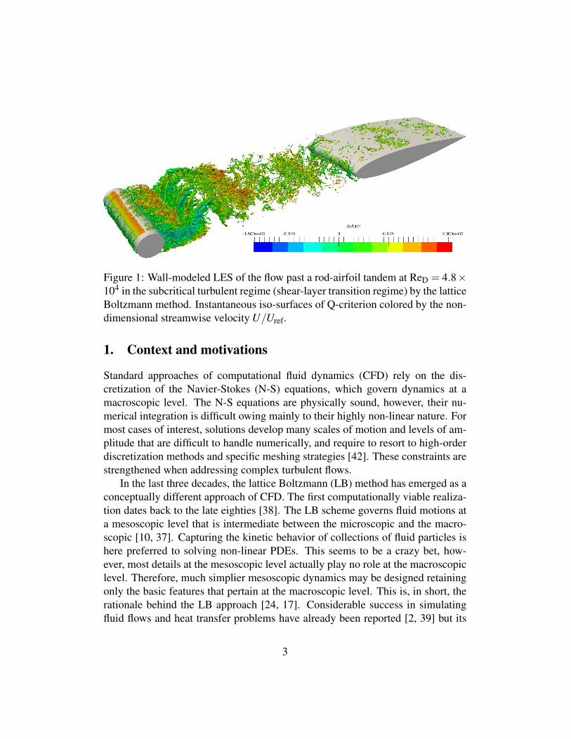
Figure 1: Wall-modeled LES of the flow past a rod-airfoil tandem at ReD = 4.8×104 in the subcritical turbulent regime (shear-layer transition regime) by the latticeBoltzmann method. Instantaneous iso-surfaces of Q-criterion colored by the non-dimensional streamwise velocity U/Uref.

1. Context and motivations

Standard approaches of computational fluid dynamics (CFD) rely on the dis-cretization of the Navier-Stokes (N-S) equations, which govern dynamics at amacroscopic level. The N-S equations are physically sound, however, their nu-merical integration is difficult owing mainly to their highly non-linear nature. Formost cases of interest, solutions develop many scales of motion and levels of am-plitude that are difficult to handle numerically, and require to resort to high-orderdiscretization methods and specific meshing strategies [42]. These constraints arestrengthened when addressing complex turbulent flows.

In the last three decades, the lattice Boltzmann (LB) method has emerged as aconceptually different approach of CFD. The first computationally viable realiza-tion dates back to the late eighties [38]. The LB scheme governs fluid motions ata mesoscopic level that is intermediate between the microscopic and the macro-scopic [10, 37]. Capturing the kinetic behavior of collections of fluid particles ishere preferred to solving non-linear PDEs. This seems to be a crazy bet, how-ever, most details at the mesoscopic level actually play no role at the macroscopiclevel. Therefore, much simplier mesoscopic dynamics may be designed retainingonly the basic features that pertain at the macroscopic level. This is, in short, therationale behind the LB approach [24, 17]. Considerable success in simulatingfluid flows and heat transfer problems have already been reported [2, 39] but its

3

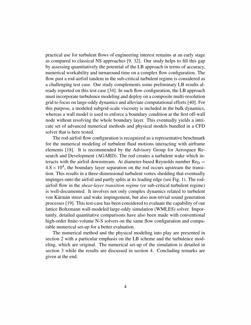
practical use for turbulent flows of engineering interest remains at an early stageas compared to classical NS approaches [9, 32]. Our study helps to fill this gapby assessing quantitatively the potential of the LB approach in terms of accuracy,numerical workability and turnaround time on a complex flow configuration. Theflow past a rod-airfoil tandem in the sub-critical turbulent regime is considered asa challenging test case. Our study complements some preliminary LB results al-ready reported on this test case [34]. In such flow configuration, the LB approachmust incorporate turbulence modeling and deploy on a composite multi-resolutiongrid to focus on large-eddy dynamics and alleviate computational efforts [40]. Forthis purpose, a modeled subgrid-scale viscosity is included in the bulk dynamics,whereas a wall model is used to enforce a boundary condition at the first off-wallnode without resolving the whole boundary layer. This eventually yields a intri-cate set of advanced numerical methods and physical models bundled in a CFDsolver that is here tested.

The rod-airfoil flow configuration is recognized as a representative benchmarkfor the numerical modeling of turbulent fluid motions interacting with airframeelements [18]. It is recommended by the Advisory Group for Aerospace Re-search and Development (AGARD). The rod creates a turbulent wake which in-teracts with the airfoil downstream. At diameter-based Reynolds number ReD =4.8× 104, the boundary layer separation on the rod occurs upstream the transi-tion. This results in a three-dimensional turbulent vortex shedding that eventuallyimpinges onto the airfoil and partly splits at its leading edge (see Fig. 1). The rod-airfoil flow in the shear-layer transition regime (or sub-critical turbulent regime)is well-documented. It involves not only complex dynamics related to turbulentvon Karman street and wake impingement, but also non-trivial sound generationprocesses [19]. This test-case has been considered to evaluate the capability of ourlattice Boltzmann wall-modeled large-eddy simulation (WMLES) solver. Impor-tantly, detailed quantitative comparisons have also been made with conventionalhigh-order finite-volume N-S solvers on the same flow configuration and compa-rable numerical set-up for a better evaluation.

The numerical method and the physical modeling into play are presented insection 2 with a particular emphasis on the LB scheme and the turbulence mod-eling, which are original. The numerical set-up of the simulation is detailed insection 3 while the results are discussed in section 4. Concluding remarks aregiven at the end.

4

2. Numerical method and physical modeling

2.1 Lattice Boltzmann methodOur solver is built upon the LB principles, which offers a particle-based descrip-tion of fluid dynamics [10, 37]. Therefore, the fluid is viewed as populations offictitious particles (carrying mass) that collide and move along the links of a dis-crete Cartesian lattice. This obviously refers to a kinetic description and rigorousconnections can be established with the Boltzmann equation [36].

Usual macroscopic fluid motions are reconstructed locally by summing up thecontributions of particles moving in the different directions. The mass density ρ

and fluid momentum ρu are given at each lattice node by

ρ = ∑α

fα and ρu = ∑α

fαcα , (1)

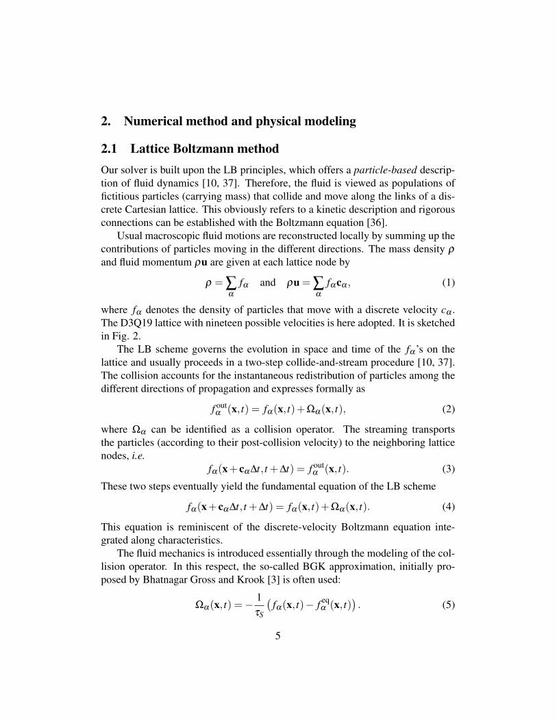
where fα denotes the density of particles that move with a discrete velocity cα .The D3Q19 lattice with nineteen possible velocities is here adopted. It is sketchedin Fig. 2.

The LB scheme governs the evolution in space and time of the fα ’s on thelattice and usually proceeds in a two-step collide-and-stream procedure [10, 37].The collision accounts for the instantaneous redistribution of particles among thedifferent directions of propagation and expresses formally as

f outα (x, t) = fα(x, t)+Ωα(x, t), (2)

where Ωα can be identified as a collision operator. The streaming transportsthe particles (according to their post-collision velocity) to the neighboring latticenodes, i.e.

fα(x+ cα∆t, t +∆t) = f outα (x, t). (3)

These two steps eventually yield the fundamental equation of the LB scheme

fα(x+ cα∆t, t +∆t) = fα(x, t)+Ωα(x, t). (4)

This equation is reminiscent of the discrete-velocity Boltzmann equation inte-grated along characteristics.

The fluid mechanics is introduced essentially through the modeling of the col-lision operator. In this respect, the so-called BGK approximation, initially pro-posed by Bhatnagar Gross and Krook [3] is often used:

Ωα(x, t) =−1τS

(fα(x, t)− f eq

α (x, t)). (5)

5

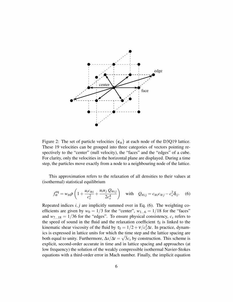
Figure 2: The set of particle velocities cα at each node of the D3Q19 lattice.These 19 velocities can be grouped into three categories of vectors pointing re-spectively to the “center” (null velocity), the “faces” and the “edges” of a cube.For clarity, only the velocities in the horizontal plane are displayed. During a timestep, the particles move exactly from a node to a neighbouring node of the lattice.

This approximation refers to the relaxation of all densities to their values at(isothermal) statistical equilibrium

f eqα = wαρ

(1+

uicα i

c2s

+uiu j Qα i j

2c4s

)with Qα i j = cα icα j− c2

s δi j. (6)

Repeated indices i, j are implicitly summed over in Eq. (6). The weighting co-efficients are given by w0 = 1/3 for the “center”, w1...6 = 1/18 for the “faces”and w7...18 = 1/36 for the “edges”. To ensure physical consistency, cs refers tothe speed of sound in the fluid and the relaxation coefficient τS is linked to thekinematic shear viscosity of the fluid by τS = 1/2+ν/c2

s ∆t. In practice, dynam-ics is expressed in lattice units for which the time step and the lattice spacing areboth equal to unity. Furthermore, ∆x/∆t =

√3cs by construction. This scheme is

explicit, second-order accurate in time and in lattice spacing and approaches (atlow frequency) the solution of the weakly compressible isothermal Navier-Stokesequations with a third-order error in Mach number. Finally, the implicit equation

6

of state for the fluid is p = ρc2s .

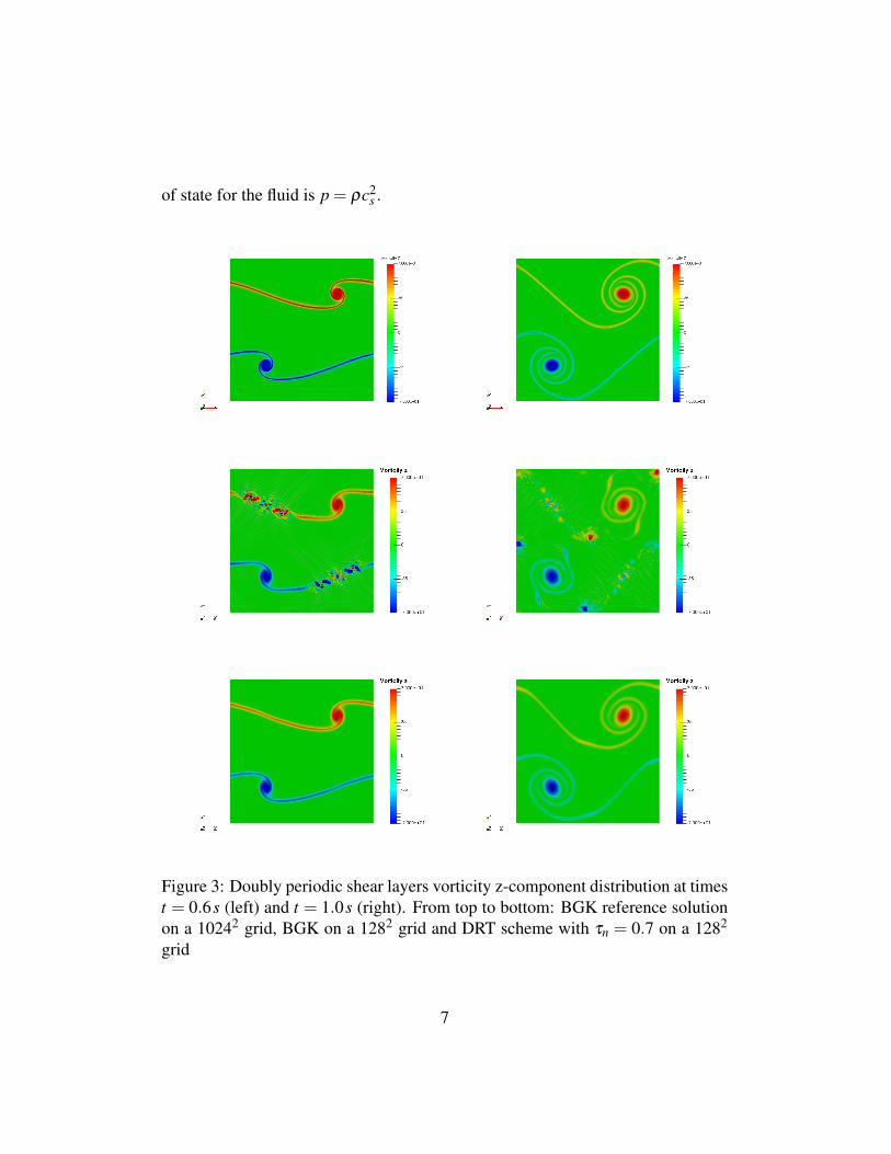
Figure 3: Doubly periodic shear layers vorticity z-component distribution at timest = 0.6s (left) and t = 1.0s (right). From top to bottom: BGK reference solutionon a 10242 grid, BGK on a 1282 grid and DRT scheme with τn = 0.7 on a 1282

grid

7

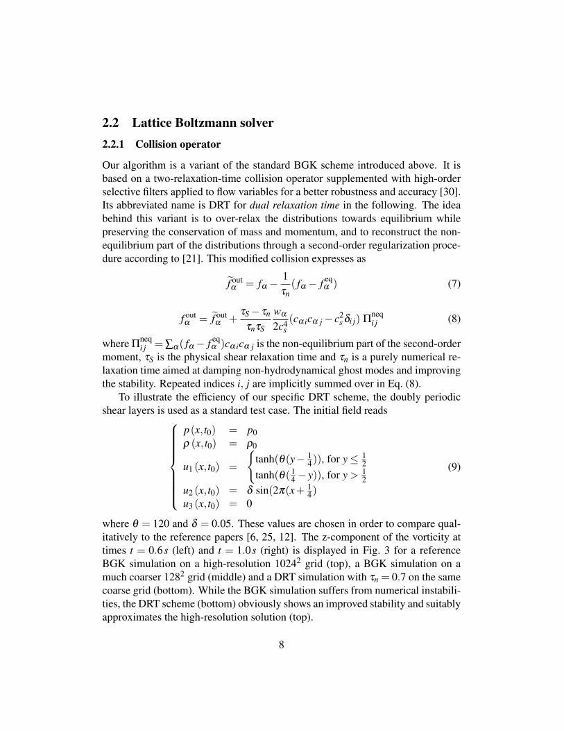
2.2 Lattice Boltzmann solver2.2.1 Collision operator

Our algorithm is a variant of the standard BGK scheme introduced above. It isbased on a two-relaxation-time collision operator supplemented with high-orderselective filters applied to flow variables for a better robustness and accuracy [30].Its abbreviated name is DRT for dual relaxation time in the following. The ideabehind this variant is to over-relax the distributions towards equilibrium whilepreserving the conservation of mass and momentum, and to reconstruct the non-equilibrium part of the distributions through a second-order regularization proce-dure according to [21]. This modified collision expresses as

f outα = fα −

1τn( fα − f eq

α ) (7)

f outα = f out

α +τS− τn

τnτS

wα

2c4s(cα icα j− c2

s δi j) Πneqi j (8)

where Πneqi j = ∑α( fα− f eq

α )cα icα j is the non-equilibrium part of the second-ordermoment, τS is the physical shear relaxation time and τn is a purely numerical re-laxation time aimed at damping non-hydrodynamical ghost modes and improvingthe stability. Repeated indices i, j are implicitly summed over in Eq. (8).

To illustrate the efficiency of our specific DRT scheme, the doubly periodicshear layers is used as a standard test case. The initial field reads

p(x, t0) = p0ρ (x, t0) = ρ0

u1 (x, t0) =

tanh(θ(y− 1

4)), for y≤ 12

tanh(θ(14 − y)), for y > 1

2u2 (x, t0) = δ sin(2π(x+ 1

4)u3 (x, t0) = 0

(9)

where θ = 120 and δ = 0.05. These values are chosen in order to compare qual-itatively to the reference papers [6, 25, 12]. The z-component of the vorticity attimes t = 0.6s (left) and t = 1.0s (right) is displayed in Fig. 3 for a referenceBGK simulation on a high-resolution 10242 grid (top), a BGK simulation on amuch coarser 1282 grid (middle) and a DRT simulation with τn = 0.7 on the samecoarse grid (bottom). While the BGK simulation suffers from numerical instabili-ties, the DRT scheme (bottom) obviously shows an improved stability and suitablyapproximates the high-resolution solution (top).

8

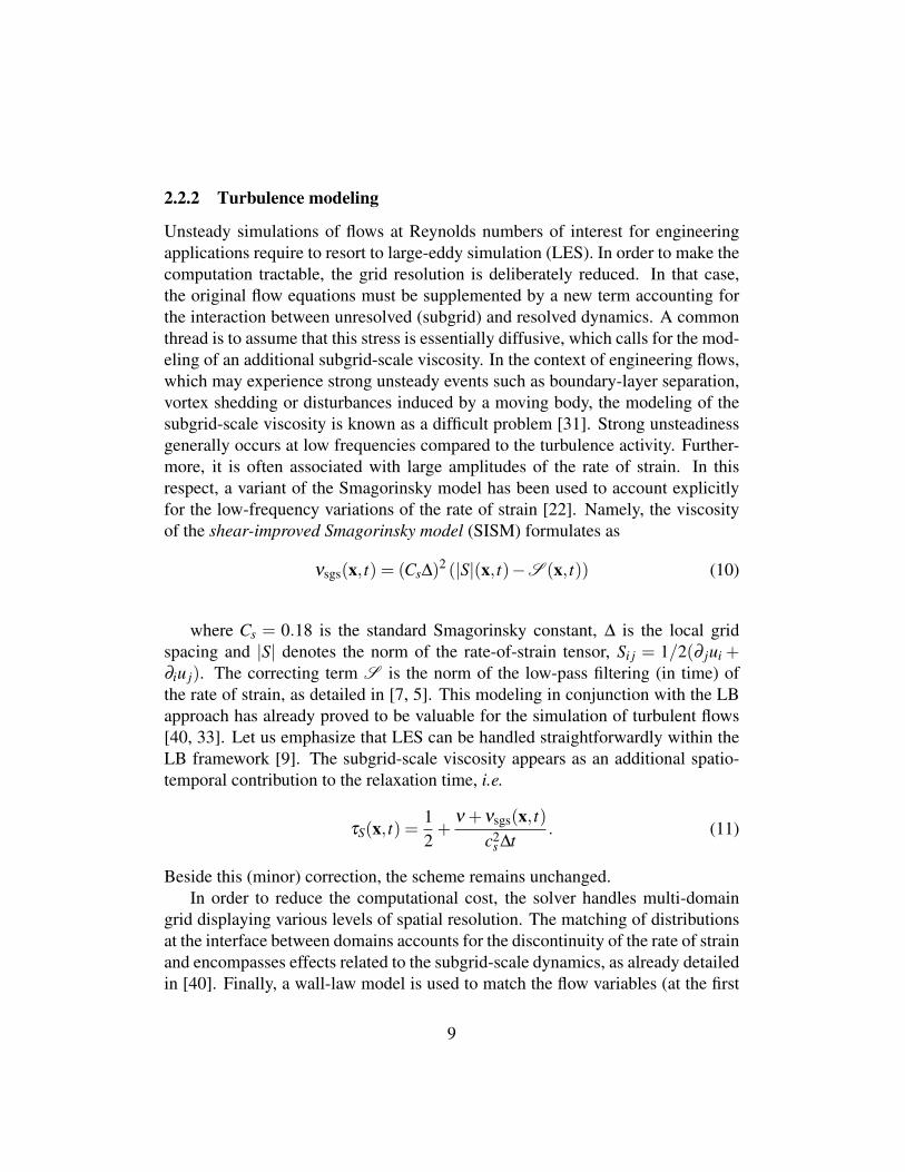
2.2.2 Turbulence modeling

Unsteady simulations of flows at Reynolds numbers of interest for engineeringapplications require to resort to large-eddy simulation (LES). In order to make thecomputation tractable, the grid resolution is deliberately reduced. In that case,the original flow equations must be supplemented by a new term accounting forthe interaction between unresolved (subgrid) and resolved dynamics. A commonthread is to assume that this stress is essentially diffusive, which calls for the mod-eling of an additional subgrid-scale viscosity. In the context of engineering flows,which may experience strong unsteady events such as boundary-layer separation,vortex shedding or disturbances induced by a moving body, the modeling of thesubgrid-scale viscosity is known as a difficult problem [31]. Strong unsteadinessgenerally occurs at low frequencies compared to the turbulence activity. Further-more, it is often associated with large amplitudes of the rate of strain. In thisrespect, a variant of the Smagorinsky model has been used to account explicitlyfor the low-frequency variations of the rate of strain [22]. Namely, the viscosityof the shear-improved Smagorinsky model (SISM) formulates as

νsgs(x, t) = (Cs∆)2 (|S|(x, t)−S (x, t)) (10)

where Cs = 0.18 is the standard Smagorinsky constant, ∆ is the local gridspacing and |S| denotes the norm of the rate-of-strain tensor, Si j = 1/2(∂ jui +∂iu j). The correcting term S is the norm of the low-pass filtering (in time) ofthe rate of strain, as detailed in [7, 5]. This modeling in conjunction with the LBapproach has already proved to be valuable for the simulation of turbulent flows[40, 33]. Let us emphasize that LES can be handled straightforwardly within theLB framework [9]. The subgrid-scale viscosity appears as an additional spatio-temporal contribution to the relaxation time, i.e.

τS(x, t) =12+

ν +νsgs(x, t)c2

s ∆t. (11)

Beside this (minor) correction, the scheme remains unchanged.In order to reduce the computational cost, the solver handles multi-domain

grid displaying various levels of spatial resolution. The matching of distributionsat the interface between domains accounts for the discontinuity of the rate of strainand encompasses effects related to the subgrid-scale dynamics, as already detailedin [40]. Finally, a wall-law model is used to match the flow variables (at the first

9

off-wall cell) with the unresolved boundary-layer dynamics [23]. Our wall lawincludes adverse-pressure-gradient effects and curvature corrections. Formally,

U+(y+) =(

1κ

logy++B)+ correcting terms. (12)

All details about the wall-law modeling may be found in [1, 29]. The reconstruc-tion (at the boundary) of particle densities from flow variables accounts accuratelyfor the shape of the geometry [41].

3. Numerical set-up of the test case

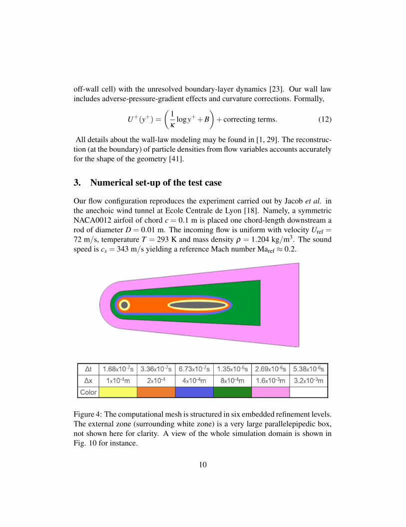
Our flow configuration reproduces the experiment carried out by Jacob et al. inthe anechoic wind tunnel at Ecole Centrale de Lyon [18]. Namely, a symmetricNACA0012 airfoil of chord c = 0.1 m is placed one chord-length downstream arod of diameter D = 0.01 m. The incoming flow is uniform with velocity Uref =72 m/s, temperature T = 293 K and mass density ρ = 1.204 kg/m3. The soundspeed is cs = 343 m/s yielding a reference Mach number Maref ≈ 0.2.

Figure 4: The computational mesh is structured in six embedded refinement levels.The external zone (surrounding white zone) is a very large parallelepipedic box,not shown here for clarity. A view of the whole simulation domain is shown inFig. 10 for instance.

10

The computational domain is structured in six embedded zones refined byoctree [40] with increasing resolution when approaching the rod and the airfoil(see Fig. 4). The overall number of cubic cells is approximatively 20×106. Thegrid resolution fulfills usual standards for LES [31]. The domain is periodic in thespanwise direction and extends over 0.35 chord length. Friction-less conditionsare used for the top and bottom boundaries. Let us mention that the external mesh(white zone) is here not sufficiently broad to allow sound waves to propagate tothe far field.

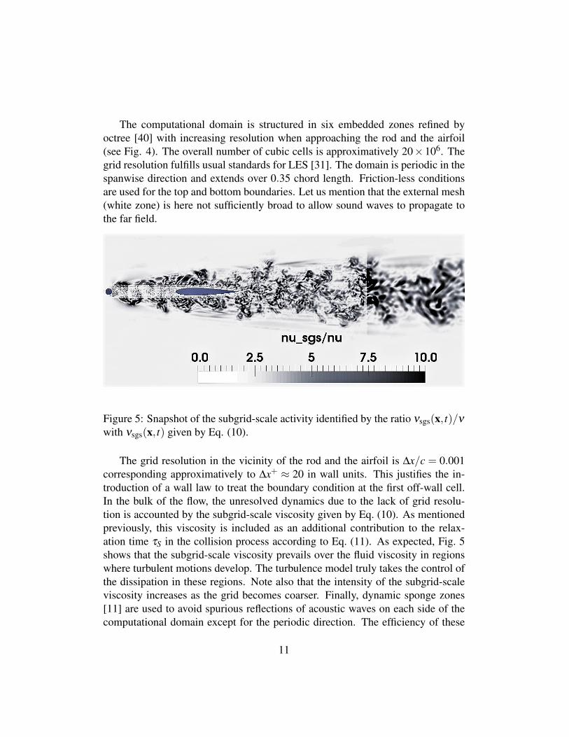
Figure 5: Snapshot of the subgrid-scale activity identified by the ratio νsgs(x, t)/ν

with νsgs(x, t) given by Eq. (10).

The grid resolution in the vicinity of the rod and the airfoil is ∆x/c = 0.001corresponding approximatively to ∆x+ ≈ 20 in wall units. This justifies the in-troduction of a wall law to treat the boundary condition at the first off-wall cell.In the bulk of the flow, the unresolved dynamics due to the lack of grid resolu-tion is accounted by the subgrid-scale viscosity given by Eq. (10). As mentionedpreviously, this viscosity is included as an additional contribution to the relax-ation time τS in the collision process according to Eq. (11). As expected, Fig. 5shows that the subgrid-scale viscosity prevails over the fluid viscosity in regionswhere turbulent motions develop. The turbulence model truly takes the control ofthe dissipation in these regions. Note also that the intensity of the subgrid-scaleviscosity increases as the grid becomes coarser. Finally, dynamic sponge zones[11] are used to avoid spurious reflections of acoustic waves on each side of thecomputational domain except for the periodic direction. The efficiency of these

11

sponge zones, where pressure fluctuations are strongly damped, is highlighted inFig. 10.

For the validation of our simulation, the results are compared with the ex-perimental measurements reported in [18] and alternative wall-resolved Navier-Stokes LES performed on the same flow configuration with the AVBP (A Very BigProject) and TurbFlow solvers. Let us mention that the mesh resolution is glob-ally higher in the two wall-resolved N-S simulations than in our wall-modeledLB simulation. The AVBP solves the compressible N-S equations on unstruc-tured grids. It relies on a third-order in space and time two-step Taylor-Galerkinscheme. A wall-adapting subgrid-scale viscosity based on the square of the ve-locity gradient tensor is used according to [26]. More details about the AVBPsolver are available in [35, 16]. The TurbFlow solver is primarily dedicated toturbomachinery flows and relies on a spatial discretization of the compressibleNS equations based on finite volumes for multiblock structured grids. Convectivefluxes are interpolated with a four-point centered scheme (fourth-order on regulargrid) and diffusive fluxes with a two-point centered scheme (second order). Timemarching relies on a five-step Runge–Kutta algorithm. The LES is handled by theSISM subgrid turbulence model as in our LB simulation. More details about theTurbFlow solver are available in [4].

The position of probes and measurement lines are identical in the experimentand simulations, as indicated in Fig. 6. Numerical samples are recorded during180 vortex-shedding periods (after the transient regime) to ensure a satisfactorystatistical convergence. The simulation is performed over 1.2×106 iterations on256 processors and lasts about 39 hours including pre and post-processing tasksof the solver. The order of magnitude of this turnaround time is excellent as com-pared to turnaround times usually encountered with conventional CFD solvers.This results mainly from the computational simplicity of the LB scheme.

4. Results of LB simulation

In this section, our results are presented. First, a qualitative analysis of the flowis carried out. Then, more quantitative comparisons are made with experimentaldata and results obtained with N-S computations on the same flow configuration.

12

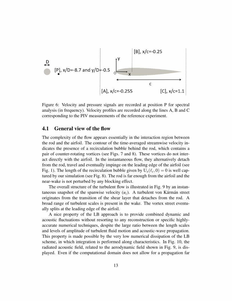
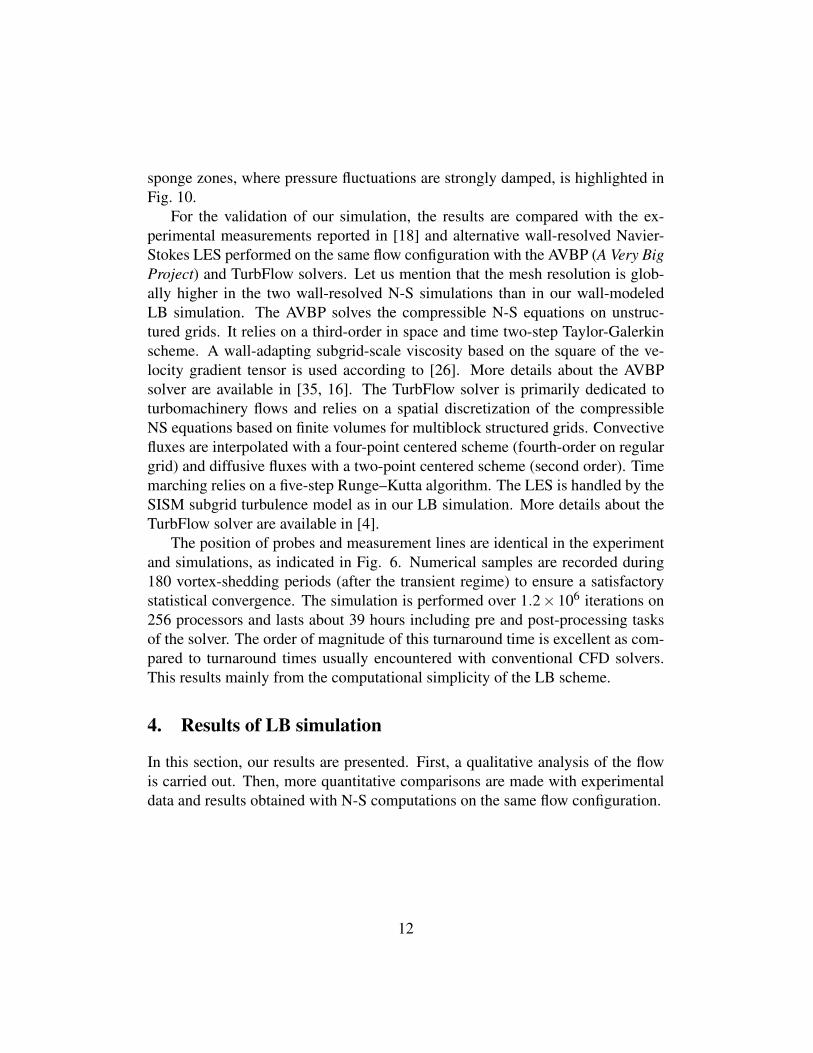
Figure 6: Velocity and pressure signals are recorded at position P for spectralanalysis (in frequency). Velocity profiles are recorded along the lines A, B and Ccorresponding to the PIV measurements of the reference experiment.

4.1 General view of the flowThe complexity of the flow appears essentially in the interaction region betweenthe rod and the airfoil. The contour of the time-averaged streamwise velocity in-dicates the presence of a recirculation bubble behind the rod, which contains apair of counter-rotating vortices (see Figs. 7 and 8). These vortices do not inter-act directly with the airfoil. In the instantaneous flow, they alternatively detachfrom the rod, travel and eventually impinge on the leading edge of the airfoil (seeFig. 1). The length of the recirculation bubble given by Ux(`c,0) = 0 is well cap-tured by our simulation (see Fig. 8). The rod is far enough from the airfoil and thenear-wake is not perturbed by any blocking effect.

The overall structure of the turbulent flow is illustrated in Fig. 9 by an instan-taneous snapshot of the spanwise velocity (uz). A turbulent von Karman streetoriginates from the transition of the shear layer that detaches from the rod. Abroad range of turbulent scales is present in the wake. The vortex street eventu-ally splits at the leading edge of the airfoil.

A nice property of the LB approach is to provide combined dynamic andacoustic fluctuations without resorting to any reconstruction or specific highly-accurate numerical techniques, despite the large ratio between the length scalesand levels of amplitude of turbulent fluid motion and acoustic-wave propagation.This property is made possible by the very low numerical dissipation of the LBscheme, in which integration is performed along characteristics. In Fig. 10, theradiated acoustic field, related to the aerodynamic field shown in Fig. 9, is dis-played. Even if the computational domain does not allow for a propagation far

13

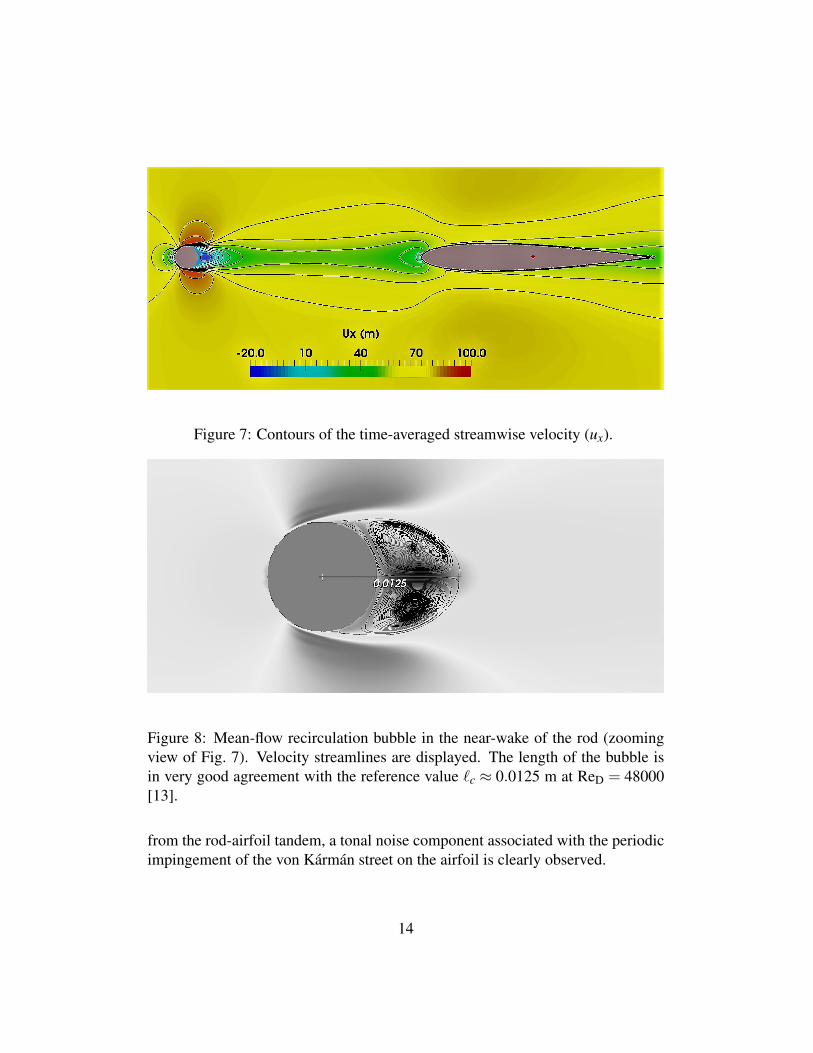
Figure 7: Contours of the time-averaged streamwise velocity (ux).

Figure 8: Mean-flow recirculation bubble in the near-wake of the rod (zoomingview of Fig. 7). Velocity streamlines are displayed. The length of the bubble isin very good agreement with the reference value `c ≈ 0.0125 m at ReD = 48000[13].

from the rod-airfoil tandem, a tonal noise component associated with the periodicimpingement of the von Karman street on the airfoil is clearly observed.

14

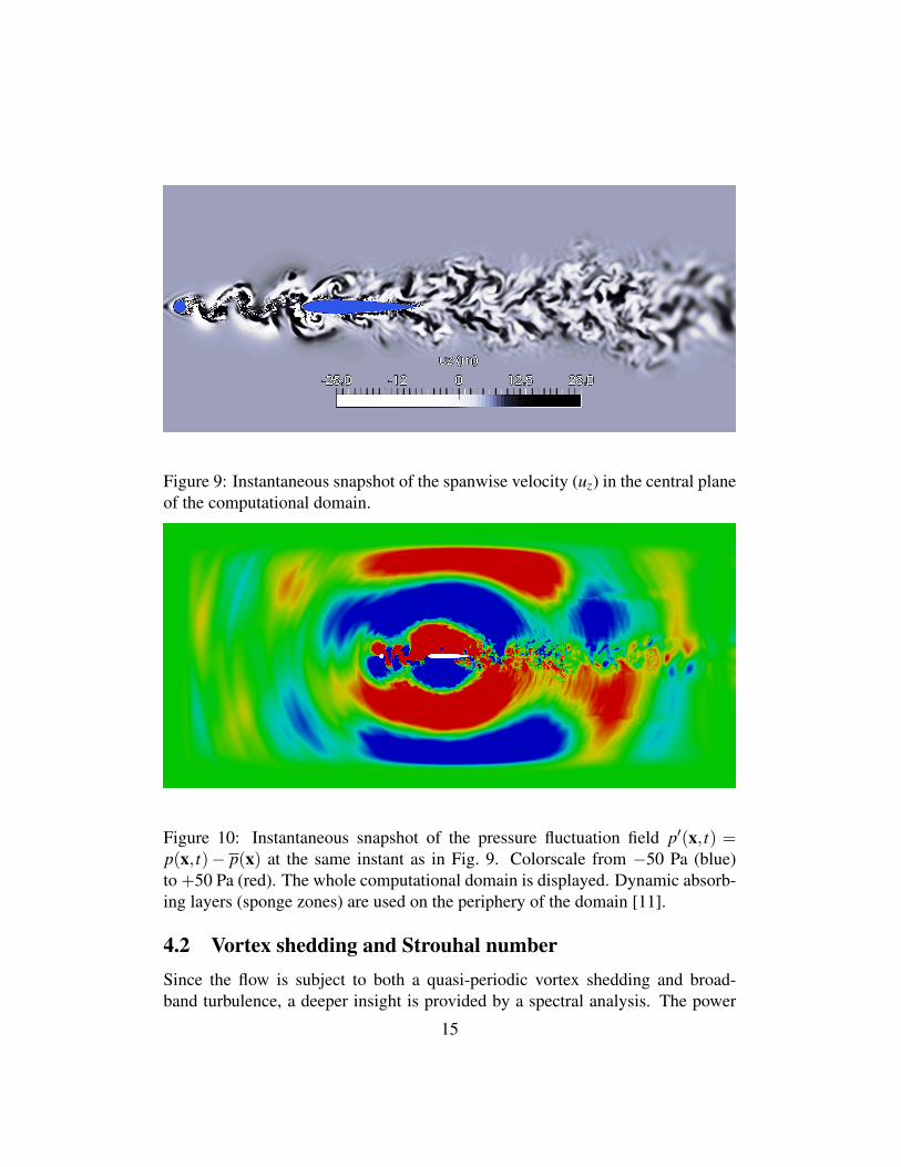
Figure 9: Instantaneous snapshot of the spanwise velocity (uz) in the central planeof the computational domain.

Figure 10: Instantaneous snapshot of the pressure fluctuation field p′(x, t) =p(x, t)− p(x) at the same instant as in Fig. 9. Colorscale from −50 Pa (blue)to +50 Pa (red). The whole computational domain is displayed. Dynamic absorb-ing layers (sponge zones) are used on the periphery of the domain [11].

4.2 Vortex shedding and Strouhal numberSince the flow is subject to both a quasi-periodic vortex shedding and broad-band turbulence, a deeper insight is provided by a spectral analysis. The power

15

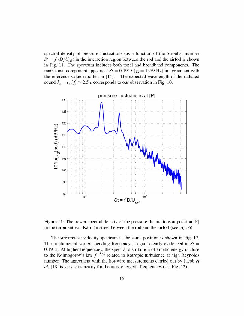
spectral density of pressure fluctuations (as a function of the Strouhal numberSt = f ·D/Uref) in the interaction region between the rod and the airfoil is shownin Fig. 11. The spectrum includes both tonal and broadband components. Themain tonal component appears at St = 0.1915 ( fs = 1379 Hz) in agreement withthe reference value reported in [14]. The expected wavelength of the radiatedsound λs = cs/ fs ≈ 2.5 c corresponds to our observation in Fig. 10.

Figure 11: The power spectral density of the pressure fluctuations at position [P]in the turbulent von Karman street between the rod and the airfoil (see Fig. 6).

The streamwise velocity spectrum at the same position is shown in Fig. 12.The fundamental vortex-shedding frequency is again clearly evidenced at St =0.1915. At higher frequencies, the spectral distribution of kinetic energy is closeto the Kolmogorov’s law f−5/3 related to isotropic turbulence at high Reynoldsnumber. The agreement with the hot-wire measurements carried out by Jacob etal. [18] is very satisfactory for the most energetic frequencies (see Fig. 12).

16

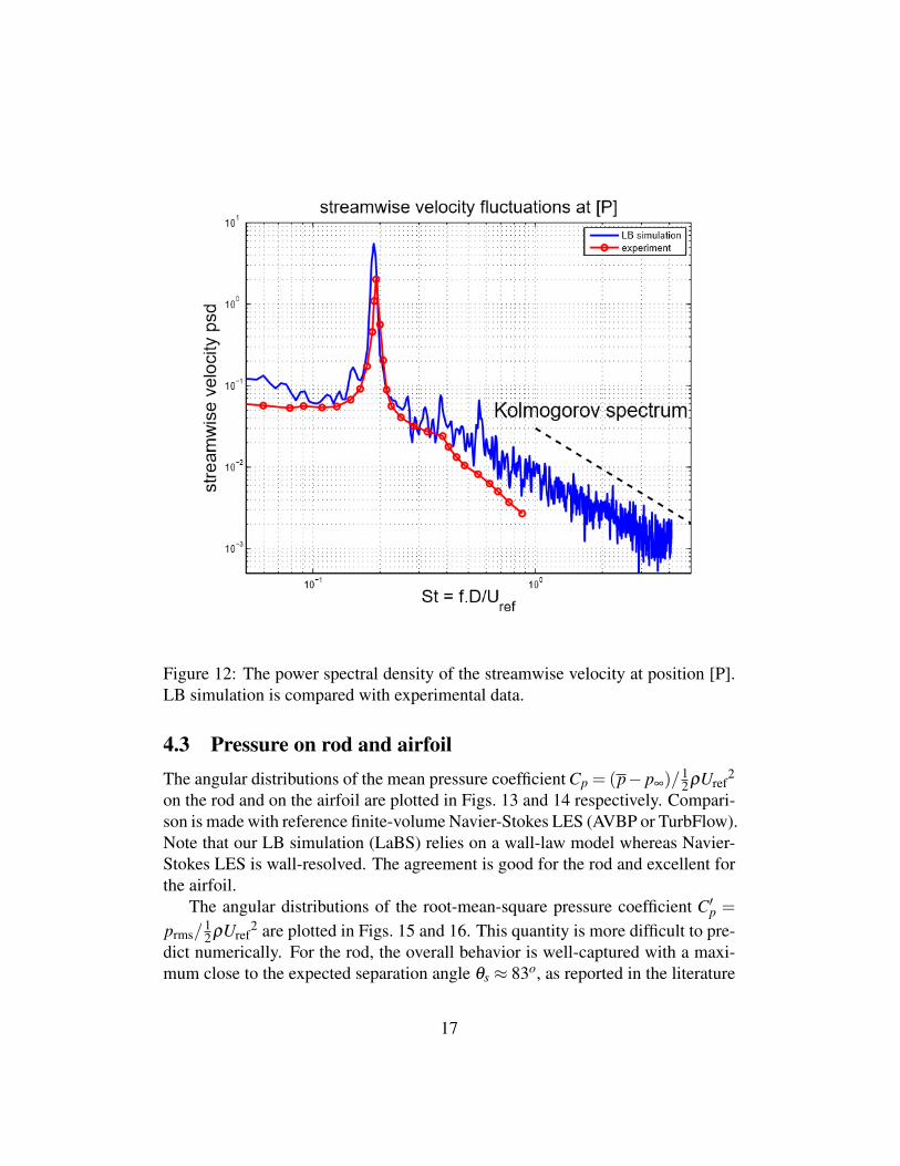
Figure 12: The power spectral density of the streamwise velocity at position [P].LB simulation is compared with experimental data.

4.3 Pressure on rod and airfoilThe angular distributions of the mean pressure coefficient Cp = (p− p∞)/

12ρUref

2

on the rod and on the airfoil are plotted in Figs. 13 and 14 respectively. Compari-son is made with reference finite-volume Navier-Stokes LES (AVBP or TurbFlow).Note that our LB simulation (LaBS) relies on a wall-law model whereas Navier-Stokes LES is wall-resolved. The agreement is good for the rod and excellent forthe airfoil.

The angular distributions of the root-mean-square pressure coefficient C′p =

prms/12ρUref

2 are plotted in Figs. 15 and 16. This quantity is more difficult to pre-dict numerically. For the rod, the overall behavior is well-captured with a maxi-mum close to the expected separation angle θs ≈ 83o, as reported in the literature

17

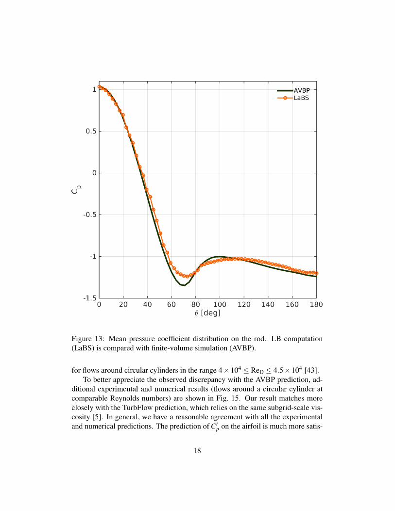
Figure 13: Mean pressure coefficient distribution on the rod. LB computation(LaBS) is compared with finite-volume simulation (AVBP).

for flows around circular cylinders in the range 4×104 ≤ ReD ≤ 4.5×104 [43].To better appreciate the observed discrepancy with the AVBP prediction, ad-

ditional experimental and numerical results (flows around a circular cylinder atcomparable Reynolds numbers) are shown in Fig. 15. Our result matches moreclosely with the TurbFlow prediction, which relies on the same subgrid-scale vis-cosity [5]. In general, we have a reasonable agreement with all the experimentaland numerical predictions. The prediction of C′p on the airfoil is much more satis-

18

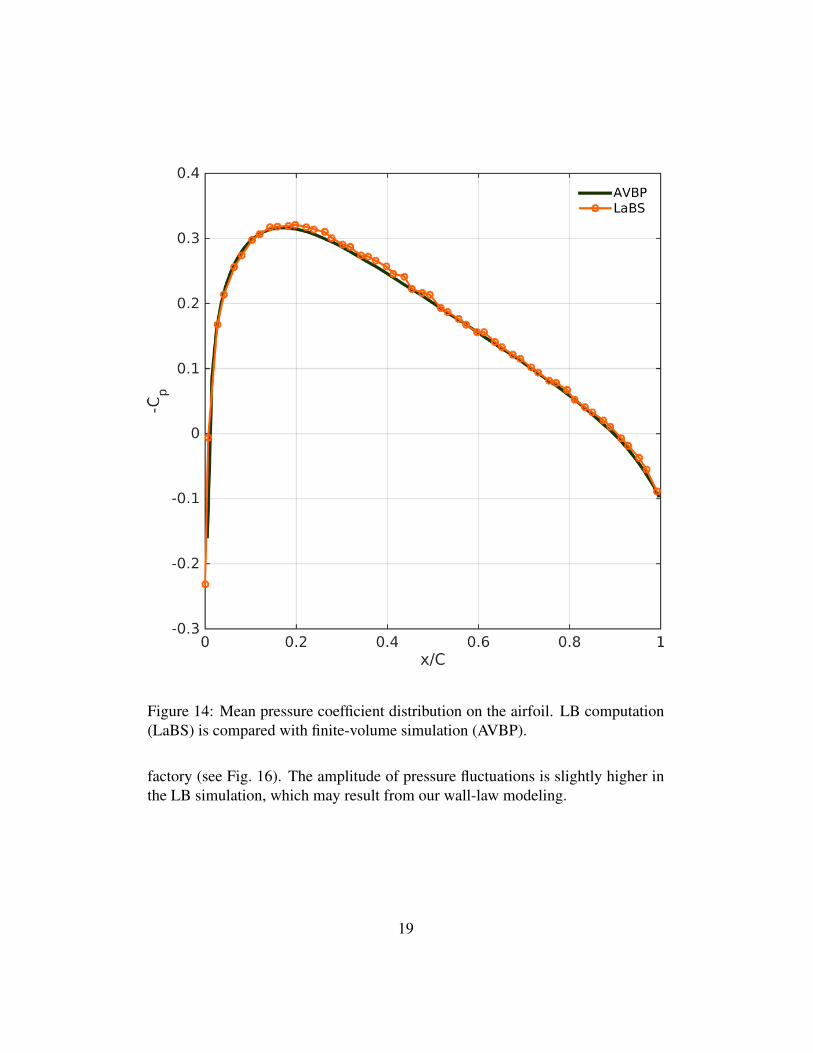
Figure 14: Mean pressure coefficient distribution on the airfoil. LB computation(LaBS) is compared with finite-volume simulation (AVBP).

factory (see Fig. 16). The amplitude of pressure fluctuations is slightly higher inthe LB simulation, which may result from our wall-law modeling.

19

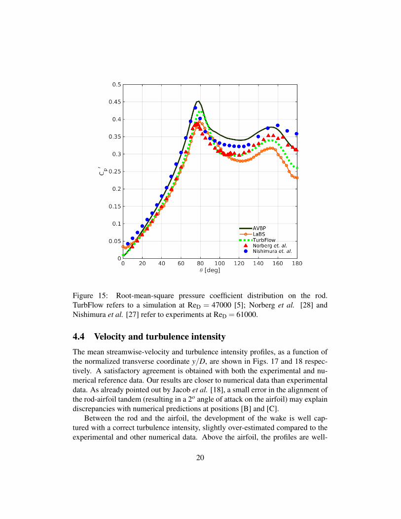
Figure 15: Root-mean-square pressure coefficient distribution on the rod.TurbFlow refers to a simulation at ReD = 47000 [5]; Norberg et al. [28] andNishimura et al. [27] refer to experiments at ReD = 61000.

4.4 Velocity and turbulence intensityThe mean streamwise-velocity and turbulence intensity profiles, as a function ofthe normalized transverse coordinate y/D, are shown in Figs. 17 and 18 respec-tively. A satisfactory agreement is obtained with both the experimental and nu-merical reference data. Our results are closer to numerical data than experimentaldata. As already pointed out by Jacob et al. [18], a small error in the alignment ofthe rod-airfoil tandem (resulting in a 2o angle of attack on the airfoil) may explaindiscrepancies with numerical predictions at positions [B] and [C].

Between the rod and the airfoil, the development of the wake is well cap-tured with a correct turbulence intensity, slightly over-estimated compared to theexperimental and other numerical data. Above the airfoil, the profiles are well-

20

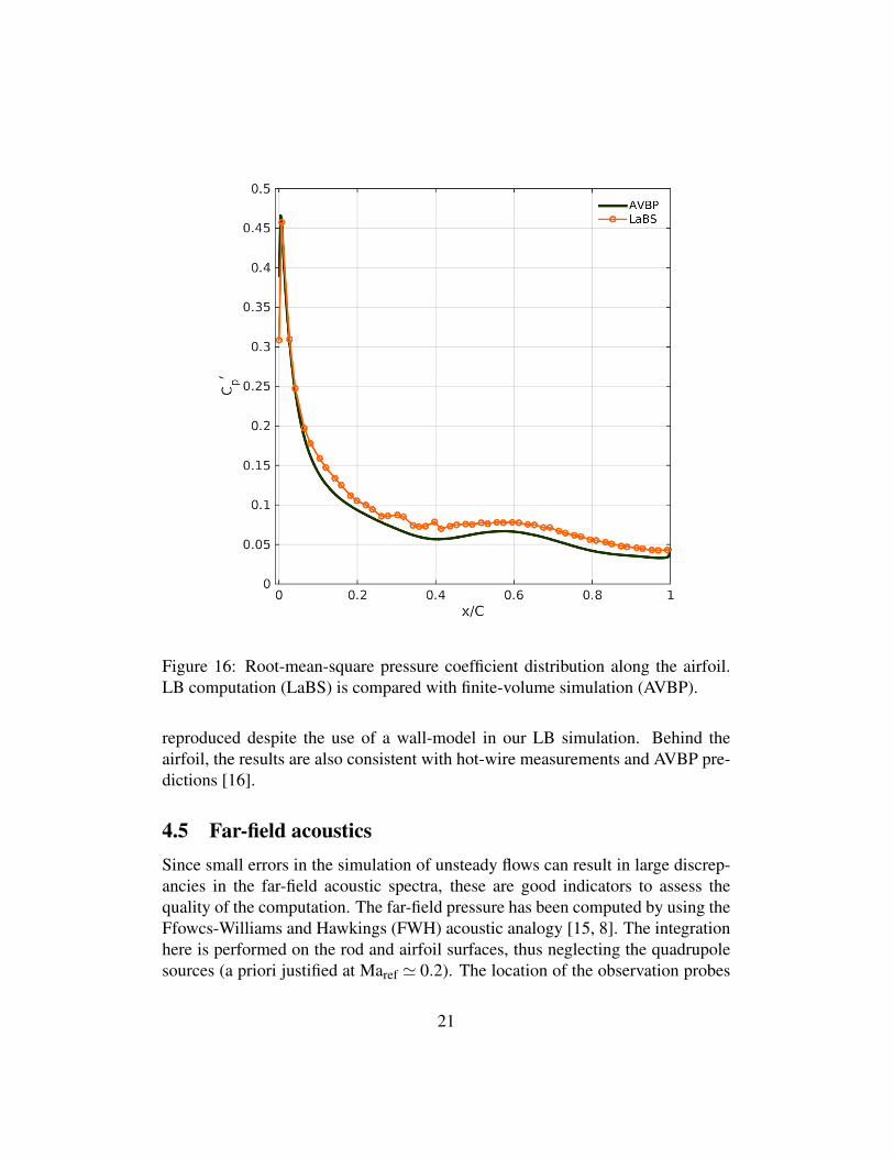
Figure 16: Root-mean-square pressure coefficient distribution along the airfoil.LB computation (LaBS) is compared with finite-volume simulation (AVBP).

reproduced despite the use of a wall-model in our LB simulation. Behind theairfoil, the results are also consistent with hot-wire measurements and AVBP pre-dictions [16].

4.5 Far-field acousticsSince small errors in the simulation of unsteady flows can result in large discrep-ancies in the far-field acoustic spectra, these are good indicators to assess thequality of the computation. The far-field pressure has been computed by using theFfowcs-Williams and Hawkings (FWH) acoustic analogy [15, 8]. The integrationhere is performed on the rod and airfoil surfaces, thus neglecting the quadrupolesources (a priori justified at Maref ' 0.2). The location of the observation probes

21

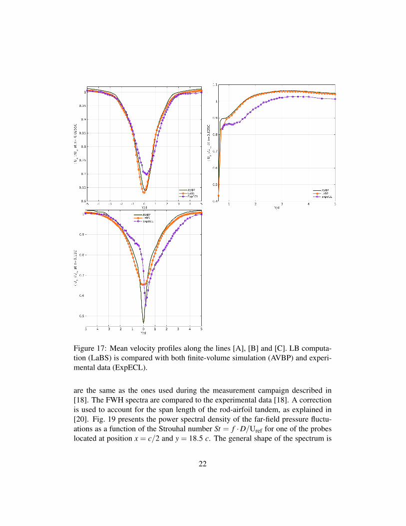
Figure 17: Mean velocity profiles along the lines [A], [B] and [C]. LB computa-tion (LaBS) is compared with both finite-volume simulation (AVBP) and experi-mental data (ExpECL).

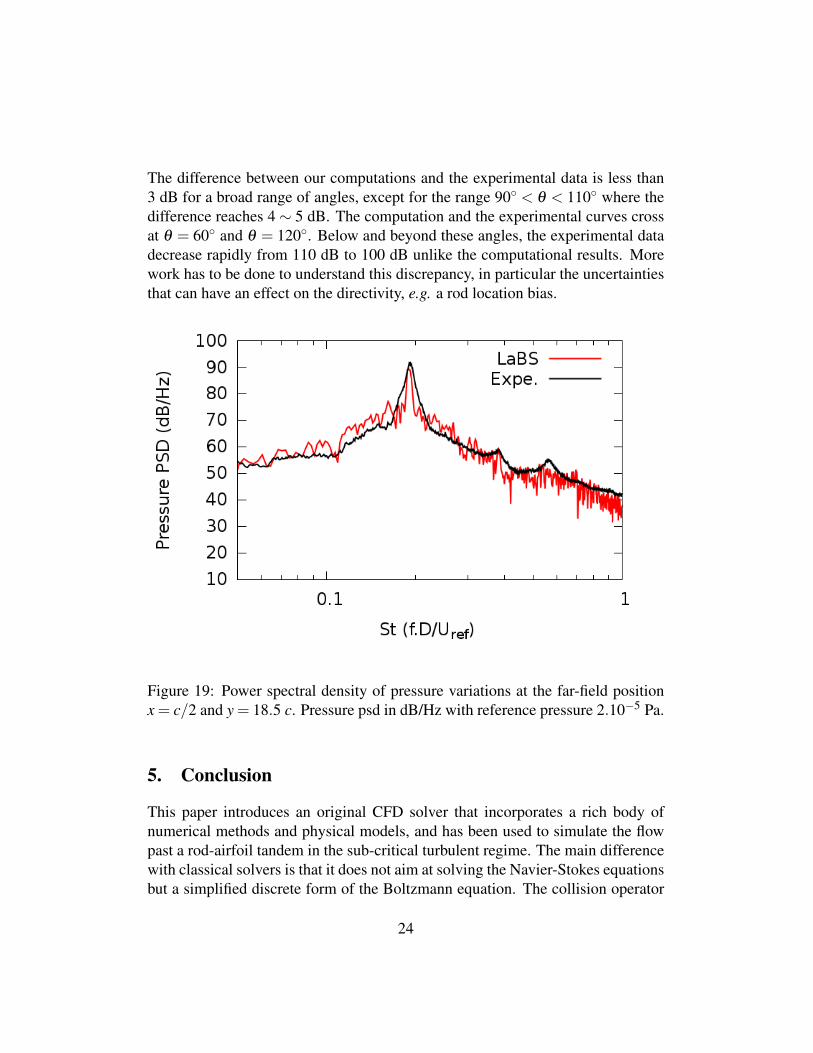
are the same as the ones used during the measurement campaign described in[18]. The FWH spectra are compared to the experimental data [18]. A correctionis used to account for the span length of the rod-airfoil tandem, as explained in[20]. Fig. 19 presents the power spectral density of the far-field pressure fluctu-ations as a function of the Strouhal number St = f ·D/Uref for one of the probeslocated at position x = c/2 and y = 18.5 c. The general shape of the spectrum is

22

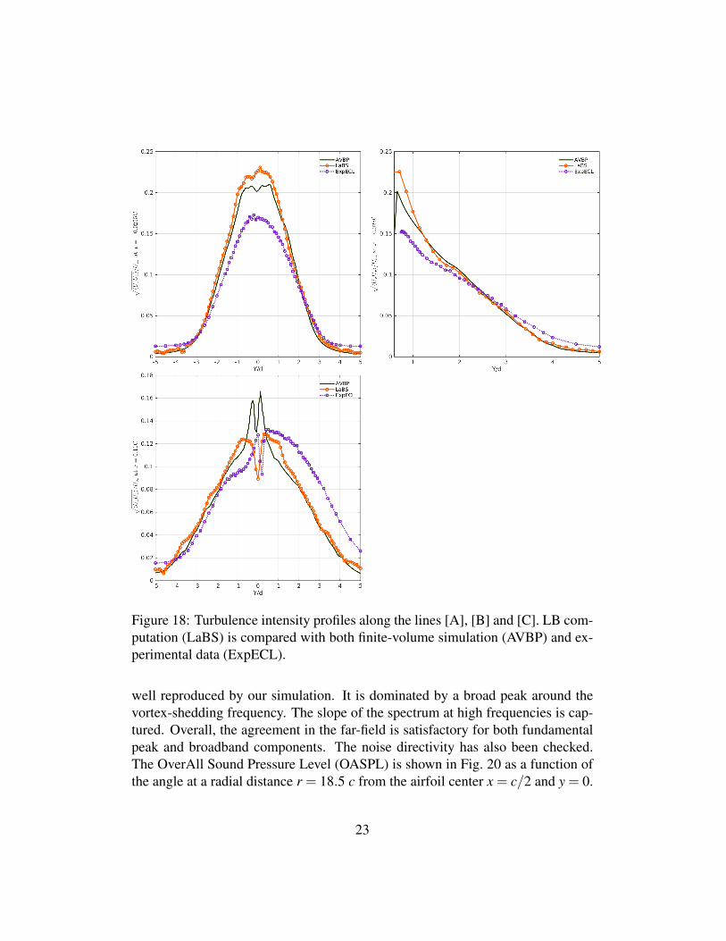
Figure 18: Turbulence intensity profiles along the lines [A], [B] and [C]. LB com-putation (LaBS) is compared with both finite-volume simulation (AVBP) and ex-perimental data (ExpECL).

well reproduced by our simulation. It is dominated by a broad peak around thevortex-shedding frequency. The slope of the spectrum at high frequencies is cap-tured. Overall, the agreement in the far-field is satisfactory for both fundamentalpeak and broadband components. The noise directivity has also been checked.The OverAll Sound Pressure Level (OASPL) is shown in Fig. 20 as a function ofthe angle at a radial distance r = 18.5 c from the airfoil center x = c/2 and y = 0.

23

The difference between our computations and the experimental data is less than3 dB for a broad range of angles, except for the range 90 < θ < 110 where thedifference reaches 4∼ 5 dB. The computation and the experimental curves crossat θ = 60 and θ = 120. Below and beyond these angles, the experimental datadecrease rapidly from 110 dB to 100 dB unlike the computational results. Morework has to be done to understand this discrepancy, in particular the uncertaintiesthat can have an effect on the directivity, e.g. a rod location bias.

Figure 19: Power spectral density of pressure variations at the far-field positionx = c/2 and y = 18.5 c. Pressure psd in dB/Hz with reference pressure 2.10−5 Pa.

5. Conclusion

This paper introduces an original CFD solver that incorporates a rich body ofnumerical methods and physical models, and has been used to simulate the flowpast a rod-airfoil tandem in the sub-critical turbulent regime. The main differencewith classical solvers is that it does not aim at solving the Navier-Stokes equationsbut a simplified discrete form of the Boltzmann equation. The collision operator

24

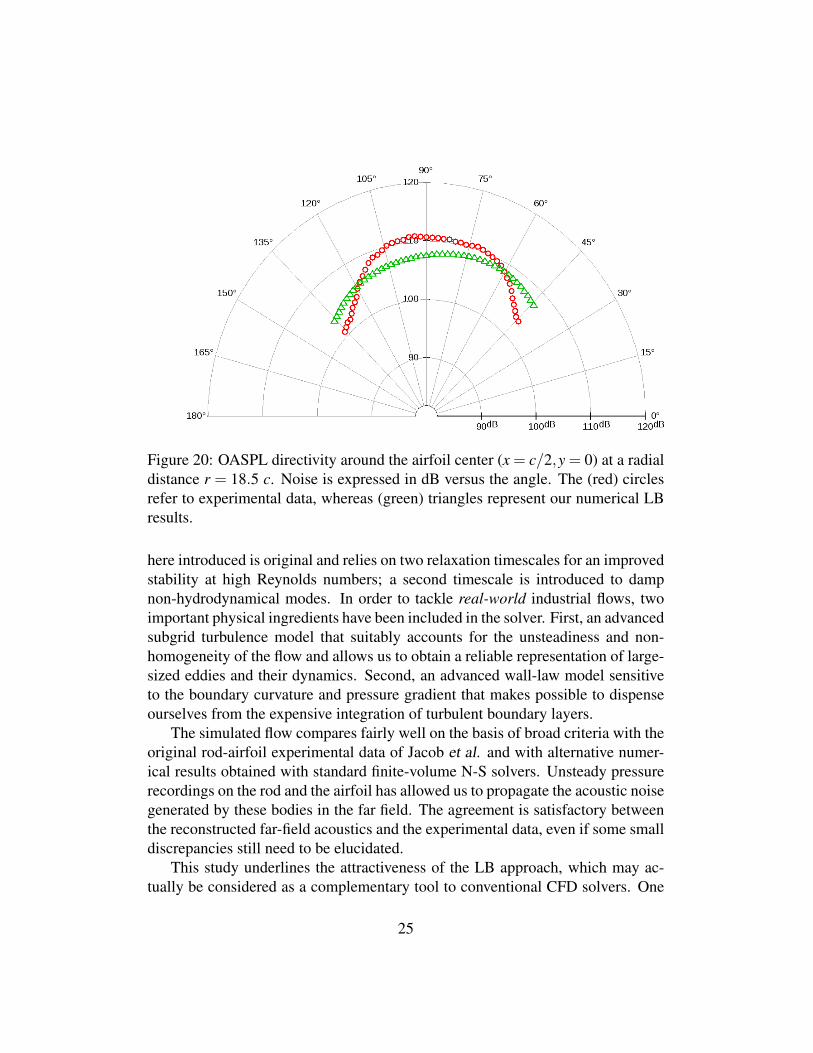
Figure 20: OASPL directivity around the airfoil center (x = c/2,y = 0) at a radialdistance r = 18.5 c. Noise is expressed in dB versus the angle. The (red) circlesrefer to experimental data, whereas (green) triangles represent our numerical LBresults.

here introduced is original and relies on two relaxation timescales for an improvedstability at high Reynolds numbers; a second timescale is introduced to dampnon-hydrodynamical modes. In order to tackle real-world industrial flows, twoimportant physical ingredients have been included in the solver. First, an advancedsubgrid turbulence model that suitably accounts for the unsteadiness and non-homogeneity of the flow and allows us to obtain a reliable representation of large-sized eddies and their dynamics. Second, an advanced wall-law model sensitiveto the boundary curvature and pressure gradient that makes possible to dispenseourselves from the expensive integration of turbulent boundary layers.

The simulated flow compares fairly well on the basis of broad criteria with theoriginal rod-airfoil experimental data of Jacob et al. and with alternative numer-ical results obtained with standard finite-volume N-S solvers. Unsteady pressurerecordings on the rod and the airfoil has allowed us to propagate the acoustic noisegenerated by these bodies in the far field. The agreement is satisfactory betweenthe reconstructed far-field acoustics and the experimental data, even if some smalldiscrepancies still need to be elucidated.

This study underlines the attractiveness of the LB approach, which may ac-tually be considered as a complementary tool to conventional CFD solvers. One

25

may highlight the capability of the LB method to encompass dynamic and acous-tic fluctuations in a simple numerical framework without resorting to any spe-cific high-order numerical techniques. Therefore, when turnaround time is a con-cern, a LB solver becomes a serious contender because of its impressive compu-tational efficiency. Finally, let us mention that the integration of more complexfluid physics is possible in the LB framework, which paves the path to efficientmulti-physics CFD solvers [38].

6. Acknowledgments

LB simulations have been performed on the local HPC facilities at Ecole Centralede Lyon (PMCS2I) and Ecole Normale Superieure de Lyon (PSMN). These HPCfacilities are supported by their academic host institutions, the Auvergne-Rhone-Alpes region (GRANT CPRT07-13 CIRA) and the national Equip@Meso grant(ANR-10-EQPX-29-01). The research work has been financially supported by theFrench Ministry of Industry and Bpifrance in the framework of the “Programmed’Investissement d’Avenir : Calcul Intensif et Simulation Numerique”. F. Chevil-lotte and F.-X. Becot (Matelys research Lab) have helped for the development ofdynamic sponge zones in the LaBS solver. We thank Basile Bazin (CS-SI) for hishelp in the mesh setting.

References

[1] N. Afzal. Wake layer in a turbulent boundary layer with pressure gradient:A new approach. IUTAM Symposium on Asymptotic Methods for TurbulentShear flows at High Reynolds Numbers, 535:95–118, 1996.

[2] C.K. Aidun and J.R. Clausen. Lattice-boltzmann method for complex flows.Annual Review of Fluid Mechanics, 42(439–472), 2010.

[3] P. L. Bhatnagar, E. P. Gross, and M. Krook. A Model for Collision Pro-cesses in Gases. I. Small Amplitude Processes in Charged and Neutral One-Component Systems. Physical Review, 94:511–525, May 1954.

[4] J. Boudet, J. Caro, L. Shao, and E. Leveque. Numerical studies towardspractical large-eddy simulations. J. Therm. Sci., 16:328, 2007.

26

[5] J. Boudet, E. Leveque, P. Borgnat, A. Cahuzac, and M.C. Jacob. A kalmanfilter adapted to the estimation of mean gradients in the large-eddy simula-tion of unsteady turbulent flows. Comput. Fluids, 127:65–77, 2016.

[6] D.L. Brown and M.L. Minion. Performance Of Under-Resolved2-Dimensional Incompressible-Flow Simulations. J. Comput. Phys.,122(1):165–183, NOV 1995.

[7] A. Cahuzac, J. Boudet, P. Borgnat, and E. Leveque. Smoothing algo-rithms for mean-flow extraction in large-eddy simulation of complex tur-bulent flows. Phys. Fluids, 22:125104, 2010.

[8] D. Casalino. An advanced time approach for acoustic analogy predictions.Journal of Sound and Vibration, 261:583–612, 2003.

[9] H. Chen, S. Kandasamy, S. Orszag, R. Shock, S. Succi, and V. Yakhot.Extended boltzmann kinetic equation for turbulent flows. Science,301:633–636, 2003.

[10] S. Chen and G.D. Doolen. Lattice Boltzmann method for fluid flows. AnnualReview of Fluid Mechanics, 30(1):329–364, 1998.

[11] F. Chevillotte and D. Ricot. Development and evaluation of non-reflectiveboundary conditions for lattice boltzmann methods. 22nd AIAA/CEASAeroacoustics Conference, AIAA 2016-2915.

[12] P.J. Dellar. Bulk and shear viscosities in lattice Boltzmann equations. Phys.Rev. E, 64(3, 1):art. no.–031203, SEP 2001.

[13] H. Djeridi, M. Braza, R. Perrin, G. Harran, E. Cid, and S. Cazin. Near-waketurbulence properties around a circular cylinder at high reynolds number.Flow Turbul. Combust., 71:19, 2003.

[14] A. Eltaweel and M. Wang. Numerical simulation of broadband noise fromairfoil-wake interaction. 17th AIAA/CEAS Aeroacoustics Conference, AIAA2011-2802.

[15] J. E. Ffowcs-Williams and D. L. Hawkings. Sound generated by turbulenceand surfaces in arbitrary motion. Philosophical Transactions of the RoyalSociety A, 264:321–342, 1969.

27

[16] J. C. Giret, A. Sengissen, S. Moreau, M. Sanjose, and J.-C. Jouhaud. Noisesource analysis of a rod-airfoil configuration using unstructured large-eddysimulation. AIAA Journal, 53 (4):1062–1077, 2015.

[17] F. Higuera, S. Succi, and R. Benzi. Lattice gas-dynamics with enhancedcollisions. Europhys. Lett., 9(4):345–349, 1989.

[18] M.C. Jacob, J. Boudet, J. Casalino, and M. Michard. A rod-airfoil exper-iment as benchmark for broadband noise modeling. J. Theoret. Comput.Fluid Dyn., 19 (3):171, 2005.

[19] Y. Jiang, M.-L. Mao, X.-G. Deng, and H.-Y Liu. Numerical investigation onbody-wake flow interaction over rod-airfoil configuration. J. Fluid Mech.,779:1–35, 2015.

[20] C. Kato and M. Ikegawa. Large eddy simulation of unsteady turbulent wakeof a circular cylinder using the finite element method. Advances in Numeri-cal Simulation of Turbulent Flows, 1:49–56, 1991.

[21] J. Latt and B. Chopard. Lattice boltzmann method with regularized precol-lision distribution functions. Math. Comput. Simul., 72:165–168, 2006.

[22] E. Leveque, F. Toschi, L. Shao, and J.-P. Bertoglio. Shear-improvedsmagorinsky model for large-eddy simulation of wall-bounded turbulentflows. J. Fluid Mech., 570:491–502, 2007.

[23] O. Malaspinas and P. Sagaut. Wall model for large-eddy simulation basedon the lattice boltzmann method. J. Comput. Phys., 275:25–40, 2014.

[24] G.R. McNamara and G. Zanetti. Use of the boltzmann equation to simulatelattice-gas automata. Phys. Rev. Lett., 61:2332–2335, 1988.

[25] M.L. Minion and D.L. Brown. Performance of under-resolved two-dimensional incompressible flow simulations, II. J. Comput. Phys.,138(2):734–765, DEC 1997.

[26] F. Nicoud and F. Ducros. Subgrid-scale stress modelling based on the squareof the velocity gradient tensor. Flow Turbul. Combust., 62(3):183–200,1999.

[27] H. Nishimura and Y. Taniike. Aerodynamic characteristics of fluctuatingforces on a circular sylinder. J. Wind Eng Ind Aerodyn, 89:713–723, 2001.

28

[28] C. Norberg. Fluctuating lift on a circular cylinder: review and new measure-ments. J. Fluids Struct, 17:57–96, 2003.

[29] V. C. Patel and F. Sotiropoulos. Longitudinal curvature effects in turbulentboundary layer. Prog. Aerospace Sci., 33 (1-2):1–70, 1997.

[30] D. Ricot, S. Marie, P. Sagaut, and C. Bailly. Lattice boltzmann method withselective viscosity filter. J. Comput. Phys., 228:4478–4490, 2009.

[31] P. Sagaut. Large eddy simulation for incompressible flows: An introduction.Springer-Verlag Berlin Heidelberg, 2006.

[32] P. Sagaut. Towards advanced subgrid models for lattice-boltzmann-basedlarge-eddy simulation: theoretical formulation. Computers and Mathematicswith Applications, 59(2194-2199), 2010.

[33] H. Sajjadia, M. Salmanzadeha, G. Ahmadib, and S. Jafaric. Simulationsof indoor airflow and particle dispersion and deposition by the lattice boltz-mann method using les and rans approaches. Build. Environ., 102:1–12,2016.

[34] Rajani Satti, Phoi-Tack Lew, Yanbing Li, Richard Shock, and Swen Noelt-ing. Unsteady flow computations and noise predictions on a rod-airfoil usinglattice boltzmann method. 47th AIAA Aerospace Sciences Meeting IncludingThe New Horizons Forum and Aerospace Exposition, AIAA 2009-497.

[35] T. Schonfeld and M. Rudgyard. Steady and unsteady flows simulations usingthe hybrid flow solver avbp. AIAA Journal, 37(11):1378–1385, 1999.

[36] Xiaowen Shan and Xiaoyi He. Discretization of the velocity space in thesolution of the boltzmann equation. Phys. Rev. Lett., 80:65–68, 1998.

[37] S. Succi. The Lattice Boltzmann Equation for Fluid Dynamics and Beyond.Clarendon, 2001.

[38] S. Succi. Lattice boltzmann 2038. Euro. Phys. Lett., 109:50001, 2015.

[39] Michael Sukop and Daniel Thorne. Lattice Boltzmann Modeling. Springer,Berlin, Heidelberg, 2006.

29

[40] H. Touil, D. Ricot, and E. Leveque. Direct and large-eddy simulation ofturbulent flows on composite multi-resolution grids by the lattice boltzmannmethod. J. Comput. Phys., 256:220–233, 2014.

[41] J. C. G. Verschaeve and B. Muller. A curved no-slip boundary condition forthe lattice boltzmann method. J. Comput. Phys., 228:4478–4490, 2010.

[42] Z.J. Wang, Krzysztof Fidkowski, Remi Abgrall, Francesco Bassi, DoruCaraeni, Andrew Cary, Herman Deconinck, Ralf Hartmann, Koen Hille-waert, H.T. Huynh, Norbert Kroll, Georg May, Per-Olof Persson, Bram vanLeer, and Miguel Visbal. High-order cfd methods: Current status and per-spective. Int. J. Numer. Meth. Fluids, 00:1–42, 2012.

[43] M. M. Zdravkovich. Flow around circular cylinders. Oxford UniversityPress, 2002.

30