Viscous bubbly flows simulation with an interface SPH model

Viscous bubbly flows simulation with an interface SPH

model

N. Greniera,∗, D. Le Touzea, A. Colagrossib,c, M. Antuonob, G.Colicchiob,c

aLUNAM Universite, Ecole Centrale Nantes, LHEEA Lab. (UMR CNRS), Nantes,France

bCNR-INSEAN, The Italian Ship Model Basin, Roma, ItalycCentre of Excellence for Ship and Ocean Structures, CeSOS/AMOS, NTNU,

Trondheim, Norway

Abstract

The multi-fluid SPH formulation by Grenier et al. (2009) is extended to study

practical problems where bubbly flows play an important role for production

processes of the offshore industry. Since these flows are dominated by viscous

and surface tension effects, the proposed formulation includes specific models

of these physical effects and validations on specific benchmark test cases are

carefully performed. The numerical outputs are validated against analytical

and numerical reference solutions, and accuracy and convergence of the

proposed numerical model are assessed. This model is then used to simulate

viscous incompressible bubbly flows of increasing complexity. These flows

include the evolution of isolated bubbles, the merging of two bubbles, and

the separation process in a bubbly flow. In each case, results are compared to

reference solutions and the influence of the Bond number on these interfacial

flow evolutions is investigated in detail.

Key words: SPH, multi-fluid, interfacial flows, non-diffusive interface,

viscous bubbly flows, surface tension effects, oil-water separation

∗Corresponding author: [email protected]

Preprint submitted to Ocean Engineering March 15, 2013

1. Introduction

Multi-fluid flows are found in a large variety of engineering fields: ocean

engineering, oil and gas, aerospace, process, automotive. In many engineering

situations, e.g., mixing/separation, hydrodynamic impact, sloshing, engine

flows, cavitation, etc., multi-fluid flows present strong dynamics resulting

in highly-nonlinear interfacial phenomena: waves, jets, fragmentations,

reconnections. This in turn induces the coexistence of large ranges of

interface scales: from small drops, bubbles, sprays... to the domain scale.

For example, in offshore oil-water separation devices, under flow constraints

the initial bubbles of the mixed flow are fragmented into smaller ones of

radii smaller than one millimeter, before aggregating to the continuous phase

present throughout the whole domain which is more than one meter large

(see Frising et al. (2006) for a review of oil/water separation under

gravity and Laleh et al. (2012) for a review of CFD studies of such

equipment).

Numerical simulation of such flows involving a wide range of interface

scales can be divided into two categories, depending on the chosen method.

In the first category length scales are simulated up to an arbitrary scale

(usually characterizing the concerned flow) and all interface scales below that

arbitrary scale are represented through suitable models. The accuracy of this

approach relies on the models used for the under-resolved interfaces and the

exchange of information between the two levels (that is, the resolved level

and the modeled one) (see e.g. Zhang and Prosperetti (1994), Abdulkadir

and Hernandez-Perez (2010) and Slot et al. (2011) for use of CFD

packages in oil industry).

In the second category, all the interface scales are simulated up to the grid

scale, thus assuming that no interface scale smaller than the grid scale exists.

This second approach is usually referred to as direct numerical simulation

of interfacial flows. Even though it is of simpler implementation since no

2

under-resolved interface model is required, its use is restrained by computer

power, typically requiring a grid scale one order of magnitude smaller than

the smallest interface scale present in the flow (e.g. the smallest bubbles).

As a consequence, direct numerical simulation of engineering problems is

generally out of reach of current simulation tools.

For what concerns the first category, specifically conceived simulations

can be performed to assess the validity of the adopted sub-models (see

e.g. Dijkhuizen et al. (2010) for the comparison of the drag

of a single bubble between Front Tracking simulations and

experiments), especially in the context of interaction of complex

interfaces and turbulence (Vincent et al. (2008) and Duret et al.

(2012)). Further, some authors explored simplified configurations

with several bubbles (see e.g. Bunner and Tryggvason (2003);

Bonometti (2005); Tryggvason et al. (2009)).

In the context of direct numerical simulation, the Smoothed Particle

Hydrodynamics (SPH) method (see, for example, Monaghan (2012),

Violeau et al. (2007), Delorme et al. (2009), Landrini et al. (2012))

presents the key advantage of keeping the interface between two fluids

perfectly sharp, thanks to its Lagrangian nature. In fact, the SPH approach

is based on the representation of any fluid through fluid elements which are

individually followed during their Lagrangian motion, exactly preserving the

amount of matter they represent. This prevents any diffusion of interfaces,

contrary to the schemes commonly used in mesh-based methods, namely

Volume Of Fluid (VOF), Level-Set (LS), Constrained Interpolation Profile

(CIP), etc.

Notwithstanding this advantage, the derivation of a multi-fluid SPH

scheme is not straightforward since one has to carefully handle the evaluation

of the pressure gradient to density ratio in the momentum equation. In

fact, the SPH method relies on a smoothing procedure: each fluid element

3

carries its own physical quantities (e.g. density, velocity, pressure. . . ) and is

associated with a compact support which represents an interaction domain.

All the spatial differential operators are evaluated through a smoothing

procedure on this support. As a consequence, the accuracy in modeling the

discontinuous pressure gradient at an interface worsens close to this interface

since the compact support intersects this surface. Several solutions have

been proposed in the SPH community to address this issue (Tartakovsky

and Meakin (2005), Hu and Adams (2006), Price (2008), Leduc et al. (2010),

Adami et al. (2010), Khayyer and Gotoh (2012)).

A first SPH simulation of bubbly flow was carried out by Das

and Das (2009), even though surface tension effects or viscous

effects had not been carefully validated on academic test cases.

Nevertheless, the simulations of bubbly flows at coarse resolution

were compared to experimental results. Further improvements

of their scheme (with incorporation of a diffuse interface model)

allowed performing simulations with higher density ratios (Das

and Das (2011)) and exploring physical parameters (Das and Das

(2013)) of such bubbly flows. More recently, in Szewc et al.

(2013) the authors performed three dimensional simulations of

single rising bubble using the present scheme and compared their

results to experiments.

In Grenier et al. (2009) a novel SPH scheme was proposed which

overcomes this issue by providing an accurate way to evaluate the pressure

gradient to density ratio close to interfaces. To this purpose, a Shepard

kernel was adopted to recover a sharp discontinuity of the density field, which

is treated phase by phase. About the numerical scheme, we first propose

a slight improvement of the classical formulation for the Laplacian of the

velocity field: it is based on the renormalization of the standard formulation

by Morris et al. (1997) and allows for a more accurate description of the

4

viscous effects. Conversely, the surface tension effects have been modeled

accordingly to Grenier et al. (2009) (adapted from the formulation by Hu

and Adams (2006)).

After these formulations have been introduced, a careful validation of the

proposed scheme is provided on a set of academic test cases. The validation

is also made by comparison to reference solutions and by assessment of the

accuracy and convergence of the proposed method. The proposed numerical

model is then applied to bubbly flows of increasing complexity. The evolution

of isolated bubbles is first studied at low and high Bond numbers, with

comparison to reference analytical and mesh-based method solutions. Then,

the merging of two bubbles is studied and the influence of the surface tension

magnitude investigated in detail, again comparing to reference simulations.

Finally, the role played by surface tension in the oil-water separation process

is analyzed on a simplified configuration where an initial set of bubbles

migrates and merge with an already separated layer of lighter fluid.

2. Numerical model

In the present section we first briefly recall the core part of the numerical

scheme used in the present paper; for a more complete description we address

the reader to the previous work by Grenier et al. (2009). Then, the viscosity

and surface tension modeling are discussed more in depth.

2.1. Governing equations

We consider a set of weakly-compressible immiscible viscous flows. The

global fluid domain Ω is then composed of different fluids A,B, etc., so that

Ω = (A ∪ B ∪ . . .). The flow evolution is governed by the Navier-Stokes

equations and the Lagrangian description is used. All the fluids are assumed

to be barotropic following Tait’s equation of state. The governing equations

5

thus read

ρDu

Dt= −∇p + FV + FS + FB

p =c20X ρ0XγX

[(

ρ

ρ0X

)γX

− 1

]

Dx

Dt= u ;

Dv

Dt= v div(u)

(1)

where X indicates a generic fluid in Ω, and c0X , ρ0X , and γX are, respectively,

its reference sound speed, density, and polytropic constant. x, u, ρ, v, and

p represent, respectively, the displacement, the velocity, the density, the

specific volume, and pressure of a generic material element of fluid X . Finally,

FV,FS,FB indicate viscous, surface tension, and body forces, respectively.

2.2. Discretization

The SPH discretization of system (1) is based on the use of a Shepard

renormalized kernel, and on a density evaluation performed separately on

each fluid so as to maintain a perfectly sharp interface (see Grenier et al.

(2009) for details). The governing equations are discretized in two steps.

First, the density and pressure of particle i are updated from the knowledge

of particle masses (constant in time) and positions through, ∀xi ∈ X

〈ρ〉i =∑

j∈X

mj WSj (xi) ; W S

j (xi) =Wj(xi)

ΓXi

ΓXi =

∑

k∈X Wk(xi)Vk

pi =c20X ρ0XγX

[(〈ρ〉iρ0X

)γX

− 1

]

(2)

where W (xi) is the SPH renormalized Gaussian kernel used in Grenier et al.

(2009) with 3h support radius centered in i (where h is the smoothing length).

6

S denotes the Shepard renormalization of the kernel, and mi the mass of

particle i. In all the following expressions, the summations apply to the

whole kernel support whatever is the fluid within it, unless specified as e.g.

in the definition of ΓXi where the summation applies only to particles of fluid

X .

In the second step, the particle volume Vi, the velocity, and the position

of the considered particle can be marched in time through

DVi

Dt= Vi

∑

j

uji ·∇Wij

Γi

Vj

Γi =∑

k Wik Vk

ρiDui

Dt= −

∑

j

(

piΓi

+pjΓj

)

∇Wij Vj + FVi + FSi + FBi

Dxi

Dt= ui

(3)

where uji = uj − ui and ∇Wij = ∇Wj(xi). Note that this scheme allows

modeling both interfaces and free surfaces, and that ΓXi = Γi if only one fluid

is considered.

2.3. Viscosity modeling

2.3.1. Renormalized Morris et al. formulation

Following Cueille (2005), we use in the present paper a renormalized

version of the Morris et al. (1997) formulation of the Laplacian operator to

model the viscous term FV. This renormalization is performed through the

evaluation of a second-order polynomial function for which the analytical

solution is known

fi(x) = r2i (x) = |x− xi|2 ; ∇2fi(x) = K (4)

7

where K = 4 in two dimensions. The Laplacian of fi(x) evaluated by the

Morris et al. formulation (MEAF) gives

Ki =∑

j

(

1

Γi

+1

Γj

)

xij · ∇Wij

r2ijfij Vj

= −∑

j

(

1

Γi+

1

Γj

)

xij · ∇Wij Vj

(5)

where xij = xi − xj . The renormalization constant is thus equal to K/Ki

and the renormalized MEAF (RMEAF) writes

FVi =K

Ki

∑

j

µij

(

1

Γi

+1

Γj

)

xij · ∇Wij

r2ijuij Vj (6)

2.3.2. Inter-particular dynamic viscosity

The inter-particular dynamic viscosity can be evaluated by using two

different formulas. The former is based on the arithmetic mean between the

viscosity of particles i and j

µij =1

2(µi + µj) (7)

The latter is based on the harmonic mean

µij =2µiµj

µi + µj

(8)

The specific formula used for the interfacial dynamic viscosity has a crucial

influence on the evolution of multi-fluid systems when µi and µj have different

orders of magnitude. If, e.g., µi ≫ µj then Eq. (7) gives µij ≃ µi/2

which is a much larger value than the the harmonic mean given by Eq. (8)

µij ≃ 2µj. This generates important differences in the numerical solution,

see Sec. 3.1.2. On the opposite, formulae (7) and (8) coincide when only one

fluid is considered.

8

2.4. Surface tension modeling

A classical model for modeling surface tension between two fluids is the

Continuous Surface Force model, see e.g. Morris (2000)

FXYSi = σ κ δI nI (9)

where δI is the Dirac function centered on the interface, κ is the local

curvature, and nI is the interface normal. This approach was chosen by

Morris (2000) but is not well suited to the SPH framework since a simple

evaluation of normals is not reliable. To overcome this problem, Hu and

Adams (2006) used a tensorial version of the formulation above. This model

is called Continuous Surface Stress (CSS) and reads

FXYSi = div(TXY

Si ) ∀i ∈ X

TXYSi = σXY 1

|∇Ci|(

|∇Ci|21−∇Ci ⊗∇Ci

)

(10)

where TXYSi is the surface stress tensor and σXY is the surface tension

coefficient between fluids X and Y . For more details, we address the

reader to the work of Grenier et al. (2009).

The CSS model is based on the fact that the interface normal can be

expressed through the color index by nI = ∇C/‖∇C‖. Substituting this

expression in Eq. (10) the tensor TXYS becomes

TXYS = σXY‖∇C‖(1− nI ⊗ nI) (11)

With some algebra, see e.g. Lafaurie et al. (1994), it comes that FXYSi =

div(TXYSi ) is then actually colinear to nI , as in Eq. (9).

As underlined by Morris (2000), a negative pressure can be induced by

the formulation above because of the non-null trace of the tensor TXYS . To

avoid this problem a corrective term was introduced in the CSS formulation

by Hu and Adams (2006). However, in our numerical tests no benefits were

9

obtained from this correction, nor disadvantages. Therefore, for consistency

we preferred to keep formulation (10) free from this correction. Besides, in

absence of the free surface, negative pressures which could occur due to this

surface tension model can be prevented by adding a background pressure to

the equation of state (which is a simpler alternative than implementing a

procedure to control tensile instabilities Monaghan (2000)).

Remark on the equation of state For weakly-compressible flows, the

choice of the speed of sound in the equation of state is driven by

the following condition (see, for example, Grenier et al. (2009)):

c0 > 10 max(|u|)Ω (12)

where the velocity is usually estimated ‘a priori’. For gravity

waves, the fluid velocity u is replaced by the wave celerity (see

Antuono et al. (2011) for more details). For flows driven by surface

tension, this characteristic velocity can be estimated through a

unity Weber number assumption (i.e., We = ρ|u|2R/σ where R is

the characteristic radius of curvature). See the Appendix for a

detailed justification.

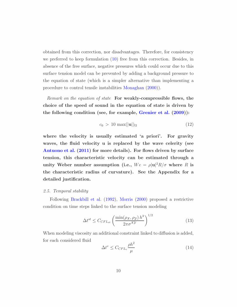
2.5. Temporal stability

Following Brackbill et al. (1992), Morris (2000) proposed a restrictive

condition on time steps linked to the surface tension modeling

∆tst ≤ CCFLst

(

min(ρX , ρY) h3

2πσXY

)1/2

(13)

When modeling viscosity an additional constraint linked to diffusion is added,

for each considered fluid

∆tv ≤ CCFLv

ρh2

µ(14)

10

Finally, the acoustic time step restriction linked to the weak compressibility

assumption reads, for each considered fluid

∆tc = CCFLcmin

i

(

h

ci + |ui|

)

(15)

As a consequence, time steps must satisfy for each considered fluid

∆t ≤ min(

∆tst,∆tv,∆tc)

(16)

Usual values for these three Courant numbers are CCFLv= 0.25, CCFLst

= 1.0

and CCFLc= 2.0 when a 4-th order Runge-Kutta time scheme is used.

3. Validation of the viscosity and surface tension models

3.1. Validation of the viscosity model

To validate the viscosity model described in Sec. 2.3, we use the Poiseuille

flow with one and two fluids (see Fig. 1). We consider a laminar viscous flow

in a planar channel of width L. The flow is driven by a pressure gradient

similar to a body force parallel to the channel axis (here the y-axis). To

reach a stationary velocity profile without increasing much the length of the

channel, we consider a periodic domain.

An analytical solution for the velocity profile can be derived. The flow is

parallel to y so that the only non-null component of the velocity field is v.

Boundary and interface conditions are, respectively: v(x = 0) = v(x = L) =

0, and vXI = vYI . For a single fluid flow the stationary velocity profile is

v(x) = −ρg

2µx(L− x) (17)

For a two-fluid flow with fluid X lying between 0 and xI and fluid Y between

xI and L, the solution is

v(x) =ρ(x)g

2µ(x)(x− xI)

2 − τIµ(x)

(x− xI)− vI (18)

11

L0

Fluid X

Velocity Profile

(a) One-fluid flow

xI

fluid Yfluid X

L0

Velocity Profilefluid Y

Velocity Profilefluid X

(b) Two-fluid flow. The

heavier and more viscous fluid

is on the left.

Figure 1: Velocity profiles in Poiseuille flows.

where the interface shear τI and velocity vI are defined by

τI =gxI2

ρXµY − ρYµX

µX + µY

vI =ρYgµY

x2I2 + τI

µY xI

(19)

Velocity profiles are extracted from a region of width equal to the channel

width and thickness equal to the mean particle distance (i.e. ∆x). The

channel is 1m× 1m and particles are initially set on a regular lattice.

The no-slip condition has been implemented through an anti-

symmetric mirroring procedure (see e.g. Macia et al. (2011)). This

choice proved to be good for relatively small Reynolds numbers.

For higher Reynolds number a different approach should be used in

order to avoid the raise of numerical instabilities. For more details

we address the reader to the works of De Leffe et al. (2011) and

Marrone et al. (2013).

12

3.1.1. One-fluid simulation

We consider a fluid with ρX = 1000 kg.m−3, µX = 1000 kg.m−1.s−1, and

choose an external acceleration of magnitude 8m.s−2. Consequently, the

maximum velocity given by Eq. (17) is equal to 1m.s−1, and the related

Reynolds number, based on the width of the channel, is equal to 1.

Accuracy of the different schemes. We set a spatial resolution of 80 particles

in the channel width and compare the viscosity model described in Sec. 2.3,

RMEAF, to three models classically employed in SPH simulations. The first

viscous formulation has been defined in Flekkøy et al. (2000) (FEAF) and

can be adapted to the present SPH formulation as follows:

FVi =∑

j

µij

2

(

1

Γi

+1

Γj

)

[xij ⊗ uij + uij ⊗ xij

r2ij

]

∇Wij Vj (20)

Another classical formulation is the one proposed by Morris et al. (1997)

(MEAF) which reads

FVi =∑

j

µij

(

1

Γi+

1

Γj

)

xij · ∇Wij

r2ijuij Vj (21)

The latter formulation is equivalent to the FEAF if the fluid is incompressible.

The third variant is the Monaghan and Gingold (1983) formulation (MGF)

which, adapted to the present formulation, reads

FVi =∑

j

KMGF

µij

2

(

1

Γi+

1

Γj

)

xij · uij

r2ij∇Wij Vj (22)

where KMGF is respectively equal to 6, 8, and 10 in one, two, and three

dimensions.

The left plot of Fig. 2 displays the relative errors in the velocity profile

at the stationary state, obtained by using the different formulations. All the

four formulations exhibit a constant error in the inner part of the channel

while larger discrepancies are observed near the solid boundaries. The

13

0 0.2 0.4 0.6 0.8 1-0.1

-0.05

0

0.05

0.1

0.15

0.2

y

errV

FEAF

MGF

MEAF

RMEAF

Exact solution

(a) Velocity relative error at t = 3 s

20 40 60 80 100 120 140 160

10-4

10-3

10-2

NerrQ

RMEAF

1st

order

2nd

order

3rd

order

(b) Spatial convergence

Figure 2: Top: relative errors of the different viscous formulations for the Poiseuille flow

at Re = 1. Bottom: spatial convergence obtained for the RMEAF (N is the number of

particles in the channel width).

corresponding root mean square errors are shown in Table 1 and show that

the MEAF is one order of magnitude more accurate than the MGF which, in

turn, is one order of magnitude more accurate than the FEAF. The RMEAF

presents the smallest error, improving the MEAF by 35%.

FEAF MGF MEAF RMEAF

errRMS 2.1 10−2 5.4 10−3 4.3 10−4 2.9 10−4

Table 1: Root-Mean-Square relative errors for the different viscous formulations tested.

In the following, the RMEAF is thus selected as the viscous formulation

of the proposed SPH scheme (see Sec. 2.3). A convergence study has been

carried out with this formulation, by varying the particle number from 20

to 160 along the channel width. The right plot of Fig.2 shows that the

14

convergence obtained with this formulation is close to the second order.

3.1.2. Two-fluid simulation

In this case an interface is present along the channel axis of symmetry,

between a lighter and a heavier fluid. The periodic channel has dimension

0.1m×0.1m, the gravity acceleration has set equal to g = 10.2m.s−2 and the

sound speed is 0.1m.s−1 for both fluids. The main parameters are reported

in Table 2.

Fluid ρ0 µ vm Re

X 1000 5 2.7 10−3 0.027

Y 100 5 10−2 7.7 10−3 0.769

Table 2: Parameters used to simulate the two-fluid Poiseuille flow (in SI units). vm is the

maximum observed velocity on which is based the mentioned Reynolds number Re.

Inter-particular dynamic viscosity. In the present section, we study how the

choice of the inter-particular dynamic viscosity formulation (see Sec. 2.3.2)

influences the accuracy of the simulations. The left plot of Fig. 3 clearly

shows that the relative error on the velocity profile is generally larger when

the arithmetic mean formulation (7) is used. Largest errors are present in the

less viscous fluid Y close to the interface with X . As explained in Sec. 2.3.2,

the use of the arithmetic mean formulation leads the inter-particular viscosity

to be approximately equal to µX/2 and this value is much greater than µY .

This implies that the Y-particles close to the interface are strongly influenced

by the X -particles, because of the SPH interpolation. Conversely, using the

harmonic mean, the X -particles close to the interface are comparatively less

influenced by the Y-particles, since the main contributions in (6) are those

of the neighbor particles belonging to fluid X .

15

0 0.2 0.4 0.6 0.8 1

-0.05

0

0.05

0.1

0.15

0.2

0.25

0.3

0.35

x/L

errV

Harmonic mean

Arithmetic mean

20 40 60 80 100 120 140 16010-4

10-3

10-2Present formulation

1st order

2nd order

3rd order

errRMS

N/L

Figure 3: Top: velocity relative error at t = 10 s, depending on the inter-particular viscosity

formulation used. Bottom: spatial convergence when using the harmonic mean formulation

(N is the number of particles in the channel width).

Concluding, the use of the harmonic mean formulation allows a better

global accuracy. The mean error throughout the channel width is about

0.2% versus 6% for the arithmetic mean formulation, while the RMS error

is 0.1% against 1.6%. The spatial convergence obtained with the harmonic

mean formulation is plotted in the right part of Fig. 3, showing again a

close-to-second-order convergence.

3.2. Validation of the surface tension model

The present section deals with the validation of the CSS surface tension

scheme developed in Sec. 2.4.

3.2.1. Parasitic currents in the static bubble case

Before any further analysis, we focus on a numerical issue related to the

use of the CSS scheme which has been widely documented in the literature:

the generation of parasitic currents at the interface, see, e.g., Brackbill et al.

16

(1992); Lafaurie et al. (1994). As already pointed out by Morris (2000),

these currents can lead to spurious deformations of the interface because of

the Lagrangian nature of the SPH scheme.

Note that in the literature several corrections have been proposed to

tackle this problem, in the framework of other numerical methods, see,

e.g., Popinet and Zaleski (1999); Torres and Brackbill (2000); Renardy and

Renardy (2002); Francois et al. (2006); Popinet (2009). The best strategies

seem to rely on an improved evaluation of the pressure gradient and

of the surface tension model and, at the same time, on a accurate

estimation of the local curvature. Future works will be devoted

to reduce such parasitic currents. In any case, we highlight that

they did not induce any appreciable inaccuracy in the applicative examples

considered here. Then, we simply quantify their strength without applying

any countermeasure. We first consider a static bubble without external

forces. Starting from the rest conditions, the equilibrium state is reached

when the surface tension volume force is balanced by the pressure gradient.

Configuration. The chosen configuration is identical to the one used in

Renardy and Renardy (2002). The computational domain size is 1m× 1m,

the space resolution is identical in both directions. The fluid bubble is a

disk centered at the middle of the computational domain and its radius is

equal to R = 0.125m. The bubble is surrounded by a fluid of same density

(ρ = 4kg.m−3) and same dynamic viscosity (µ = 1 kg.m−1.s−1) while the

surface tension coefficient is equal to σ = 0.357N.m−1. The equation of state

is linearized and the sound speed is set equal to 10m.s−1 for both fluids.

Spatial convergence. The spatial convergence of these parasitic currents is

analyzed by studying their velocity magnitude in different norms (namely,

N∞, N2, N1). Table 3 summarizes the results and shows that the magnitude

of the parasitic currents does not decay with the spatial refinement, whatever

is the norm used. A very slow convergence is observed for the N1 and N2

17

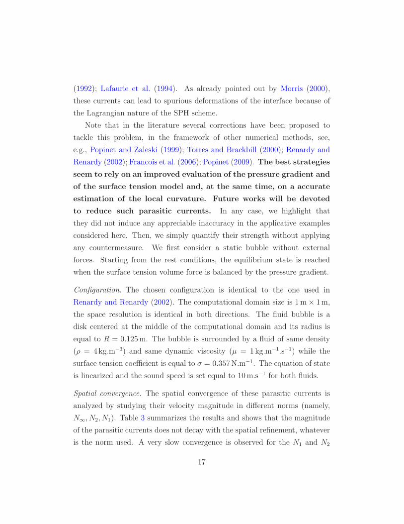
norms, and no convergence at all for the N∞ norm. This fact is illustrated

in Fig. 4 for two different spatial resolutions.

∆x/L N∞ N2 N1

1/96 1.87 10−2 1.61 10−3 3.38 10−4

1/128 1.86 10−2 1.14 10−3 2.33 10−4

1/160 2.50 10−2 1.36 10−3 2.63 10−4

1/192 1.81 10−2 1.18 10−3 2.48 10−4

Table 3: Magnitude (in m.s−1) of the parasitic current velocities at t = 2× 10−3 s for

different vectorial norms. ∆x indicates the mean inter-particle distance while L is the

fluid domain width.

This issue was also studied by Renardy and Renardy (2002) who applied

the CSS method within a Volume-Of-Fluid scheme and found a similar

behavior in terms of convergence (decrease of N1 and N2, and no decrease of

N∞). In any case, the behavior of the present scheme in terms of parasitic

currents is of relatively little importance, since they have no appreciable

influence on the dynamic test cases studied hereinafter.

For what concerns the pattern of the spurious vortices generated, it differs

from the one shown in Renardy and Renardy (2002) for both their magnitude

and their number. This is likely caused by the lower spatial accuracy of

the SPH interpolation in the estimation of curvature with respect to the

Volume-Of-Fluid method (the work of Francois et al. (2006) underlines the

importance of the numerical estimation of curvature).

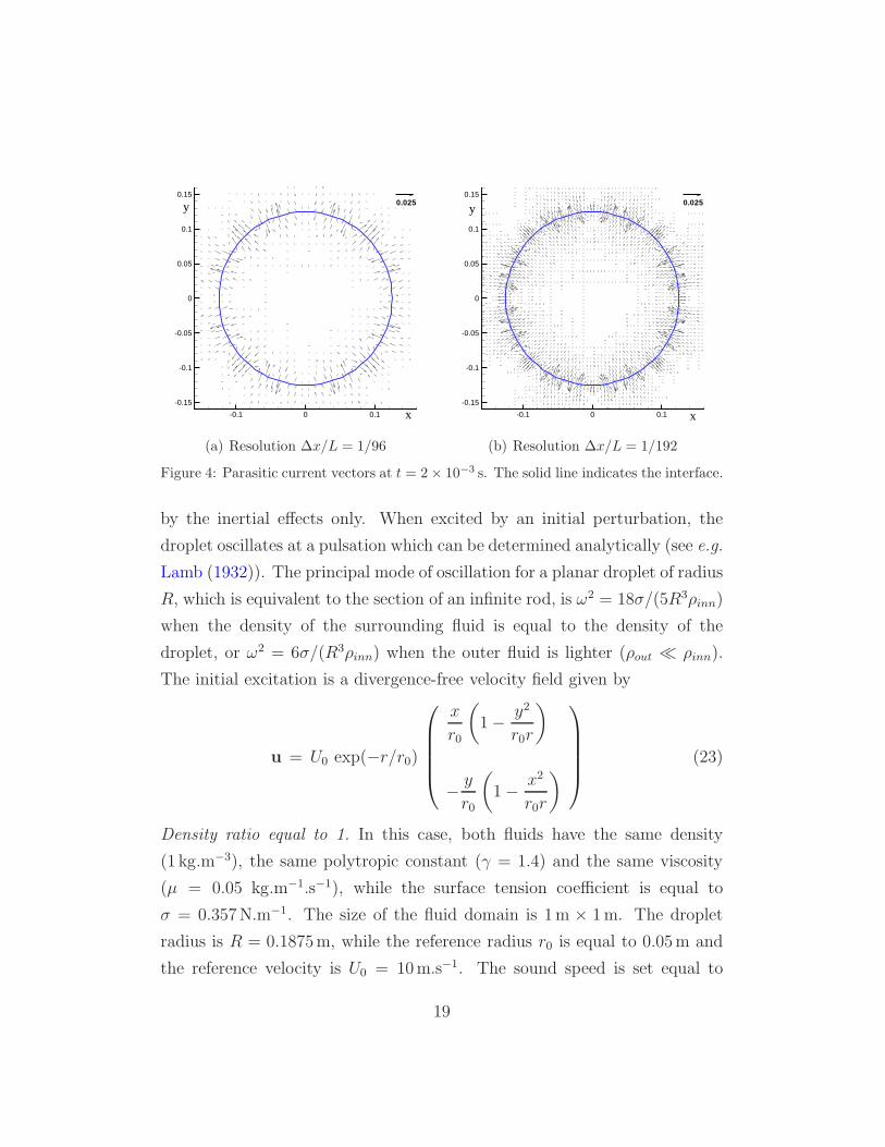
3.2.2. Oscillating droplet

To study the accuracy of the surface tension model, we perform the test of

an oscillating droplet described in Hu and Adams (2006), where no external

force is present. In this configuration, the surface tension effects are balanced

18

-0.1 0 0.1

-0.15

-0.1

-0.05

0

0.05

0.1

0.150.025

x

y

(a) Resolution ∆x/L = 1/96

-0.1 0 0.1

-0.15

-0.1

-0.05

0

0.05

0.1

0.150.025

y

x

(b) Resolution ∆x/L = 1/192

Figure 4: Parasitic current vectors at t = 2× 10−3 s. The solid line indicates the interface.

by the inertial effects only. When excited by an initial perturbation, the

droplet oscillates at a pulsation which can be determined analytically (see e.g.

Lamb (1932)). The principal mode of oscillation for a planar droplet of radius

R, which is equivalent to the section of an infinite rod, is ω2 = 18σ/(5R3ρinn)

when the density of the surrounding fluid is equal to the density of the

droplet, or ω2 = 6σ/(R3ρinn) when the outer fluid is lighter (ρout ≪ ρinn).

The initial excitation is a divergence-free velocity field given by

u = U0 exp(−r/r0)

x

r0

(

1− y2

r0r

)

− y

r0

(

1− x2

r0r

)

(23)

Density ratio equal to 1. In this case, both fluids have the same density

(1 kg.m−3), the same polytropic constant (γ = 1.4) and the same viscosity

(µ = 0.05 kg.m−1.s−1), while the surface tension coefficient is equal to

σ = 0.357N.m−1. The size of the fluid domain is 1m × 1m. The droplet

radius is R = 0.1875m, while the reference radius r0 is equal to 0.05m and

the reference velocity is U0 = 10m.s−1. The sound speed is set equal to

19

23m.s−1. To prevent the occurrence of negative values of the pressure field

and the generation of a tensile instability (cf. the work of Swegle et al.

(1995)), a background pressure value is imposed (for this test case this value

is set equal to 50Pa).

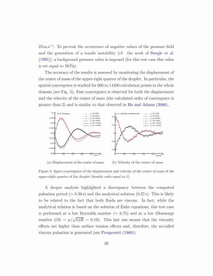
The accuracy of the results is assessed by monitoring the displacement of

the center of mass of the upper-right quarter of the droplet. In particular, the

spatial convergence is studied for 900 to 14400 calculation points in the whole

domain (see Fig. 5). Fast convergence is observed for both the displacement

and the velocity of the center of mass (the calculated order of convergence is

greater than 2) and is similar to that observed in Hu and Adams (2006).

0 0.1 0.2 0.3 0.4 0.50.06

0.065

0.07

0.075

0.08

0.085

0.09

0.095

0.1 xG (N=900)

yG (N=900)

xG (N=3600)

yG (N=3600)

xG (N=14400)

yG (N=14400)

X-Y Position

t (sec)

(a) Displacement of the center of mass

0 0.1 0.2 0.3 0.4 0.5

-0.4

-0.2

0

0.2

0.4

uG (N=900)

vG (N=900)

uG (N=3600)

vG (N=3600)

uG (N=14400)

vG (N=14400)

u-v velocity components

t (sec)

(b) Velocity of the center of mass

Figure 5: Space convergence of the displacement and velocity of the center of mass of the

upper-right quarter of the droplet (density ratio equal to 1).

A deeper analysis highlighted a discrepancy between the computed

pulsation period (∼ 0.36 s) and the analytical solution (0.27 s). This is likely

to be related to the fact that both fluids are viscous. In fact, while the

analytical relation is based on the solution of Euler equations, this test case

is performed at a low Reynolds number (∼ 0.75) and at a low Ohnesorge

number (Oh = µ/√σρR = 0.19). This last one means that the viscosity

effects are higher than surface tension effects and, therefore, the so-called

viscous pulsation is generated (see Prosperetti (1980)).

20

High density ratio. The density and viscosity of the inner fluid are now equal

to 1 kg.m−3 and µinn = 5 10−2 kg.m−1.s−1 while those of the outer fluid are

10−3 kg.m−3 and µout = 5× 10−4 kg.m−1.s−1. The polytropic coefficient γ is

equal to 1.4 for both fluids and the radius of the droplet is equal to 0.2m. To

decrease the viscosity effects (here Oh = 0.1), the initial velocity is set equal

to 1m.s−1 while r0 = 0.05m. The sound speed is chosen equal to 40m.s−1

and the background pressure equal to 50Pa.

0.6 0.8 1 1.2 1.40

0.05

0.1

0.15

0.2

0.25

0.3

0.35 τ(s), errτ

σ

Analytical Solution

Present Model

Relative Error

0.010.020.030.040.05

0.02

0.04

0.06

0.08

0.1

0.12

0.14

errτ

h (m)

Present Model

1st order

2nd order

Figure 6: Top: Comparison between the analytical and computed oscillating periods of

the oscillating bubble (high density ratio). Bottom: spatial convergence.

The numerical results are presented in Fig. 6. The pulsation of the

droplet predicted by the SPH solution is relatively close to the analytical

one, with a relative error within 3%. In the right plot of the same figure

the spatial convergence rate is evaluated showing that the present model

lies between first- and second-order of convergence. This further confirms

that the implementation of the CSS scheme in the present model allows

reproducing satisfactorily surface tension effects (this is not the case for

parasitic currents where convergence was not observed but do not play a

significant role in the bubbly flows simulated hereinafter).

21

4. Simulation of bubbly flows

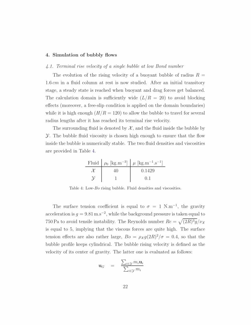
4.1. Terminal rise velocity of a single bubble at low Bond number

The evolution of the rising velocity of a buoyant bubble of radius R =

1.6 cm in a fluid column at rest is now studied. After an initial transitory

stage, a steady state is reached when buoyant and drag forces get balanced.

The calculation domain is sufficiently wide (L/R = 20) to avoid blocking

effects (moreover, a free-slip condition is applied on the domain boundaries)

while it is high enough (H/R = 120) to allow the bubble to travel for several

radius lengths after it has reached its terminal rise velocity.

The surrounding fluid is denoted by X , and the fluid inside the bubble by

Y . The bubble fluid viscosity is chosen high enough to ensure that the flow

inside the bubble is numerically stable. The two fluid densities and viscosities

are provided in Table 4.

Fluid ρ0 [kg.m−3] µ [kg.m−1.s−1]

X 40 0.1429

Y 1 0.1

Table 4: Low-Bo rising bubble. Fluid densities and viscosities.

The surface tension coefficient is equal to σ = 1 N.m−1, the gravity

acceleration is g = 9.81m.s−2, while the background pressure is taken equal to

750Pa to avoid tensile instability. The Reynolds number Re =√

(2R)3g/νX

is equal to 5, implying that the viscous forces are quite high. The surface

tension effects are also rather large, Bo = ρXg(2R)2/σ = 0.4, so that the

bubble profile keeps cylindrical. The bubble rising velocity is defined as the

velocity of its center of gravity. The latter one is evaluated as follows:

uG =

∑

i∈Y miui∑

i∈Y mi

22

4.1.1. Numerical results

The spatial convergence is studied by using the following resolutions:

h1 = 8.48× 10−3m, h2 = h1/2, and h3 = h1/4. In Fig. 7 we observe that,

0 0.5 1 1.5 2 2.5 3 3.5 4

0

0.05

0.1

0.15

0.2

0.25

vc ∞

vG (m/s)

t(sec)

R / h = 2

R/ h = 4

R/ h = 8

Figure 7: Low-Bo rising bubble. Spatial convergence of the rise velocity evolution.

for all the resolutions, the velocity converges toward an asymptotic value,

i.e. the terminal rise velocity. For this kind of configuration the dynamic

force applied by the surrounding fluid on the bubble can be compared to

the one applied on an infinite rigid cylinder in a constant velocity flow

without gravity. For a sphere, Lamb (1932) shows that the ratio between

the force applied by fluid X on a rigid solid sphere and the one applied by

the same fluid on a spherical bubble of fluid Y of the same radius is equal

to (2µX + 3µY)/(3µX + 3µY). Then, for a spherical bubble, the force ranges

in two thirds to one time the force acting on a solid sphere, depending on

the viscosity ratio between the two fluids. With the viscosities chosen here,

the force on a spherical bubble would be 80% of the one on a rigid sphere.

Unfortunately, for a cylinder the theoretical analysis of Lamb applies only to

23

-0.1 0 0.10.9

0.95

1

1.05

1.1

1.15

0.180.160.140.120.10.080.060.040.02

t=4.8 s

x (m)

y (m)| u | (m/s)

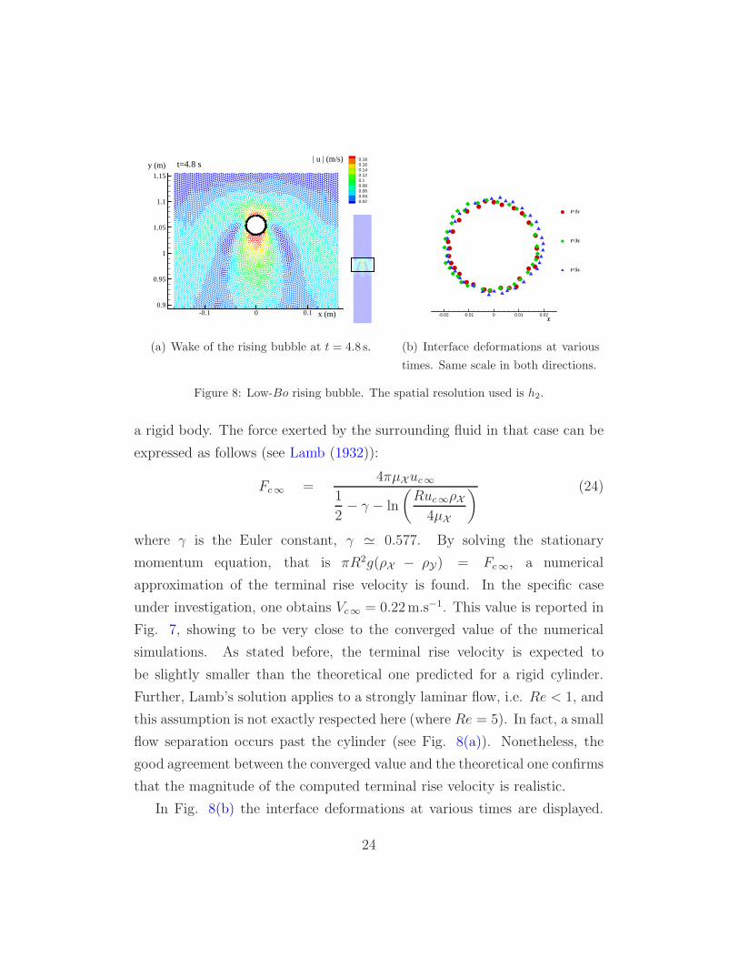
(a) Wake of the rising bubble at t = 4.8 s.

t=1s

t=3s

X-0.02 -0.01 0 0.01 0.02

t=5s

(b) Interface deformations at various

times. Same scale in both directions.

Figure 8: Low-Bo rising bubble. The spatial resolution used is h2.

a rigid body. The force exerted by the surrounding fluid in that case can be

expressed as follows (see Lamb (1932)):

Fc∞ =4πµXuc∞

1

2− γ − ln

(

Ruc∞ρX4µX

) (24)

where γ is the Euler constant, γ ≃ 0.577. By solving the stationary

momentum equation, that is πR2g(ρX − ρY) = Fc∞, a numerical

approximation of the terminal rise velocity is found. In the specific case

under investigation, one obtains Vc∞ = 0.22m.s−1. This value is reported in

Fig. 7, showing to be very close to the converged value of the numerical

simulations. As stated before, the terminal rise velocity is expected to

be slightly smaller than the theoretical one predicted for a rigid cylinder.

Further, Lamb’s solution applies to a strongly laminar flow, i.e. Re < 1, and

this assumption is not exactly respected here (where Re = 5). In fact, a small

flow separation occurs past the cylinder (see Fig. 8(a)). Nonetheless, the

good agreement between the converged value and the theoretical one confirms

that the magnitude of the computed terminal rise velocity is realistic.

In Fig. 8(b) the interface deformations at various times are displayed.

24

Y

X

Y

1.5

0.35

0.65

0 0.5 1.0

1.5R

R= 0.1

Figure 9: Two merging bubbles for Bo = ∞. Left: initial configuration. Middle and right:

contours of the vertical velocity at t = 1.90√

R/g and t = 3.16√

R/g of the present SPH

scheme.

The slight x-displacement is due to the weak non-stationarity of the flow

which induces random horizontal displacements. Nevertheless, the bubble

keeps approximately circular, proving the ability of the CSS scheme to

reproduce high surface tension effects.

4.2. Merging of two bubbles

In this section we deal with the merging of two bubbles of a light fluid

within an heavy one. A sketch of the configuration is displayed in the left

panel of Fig. 9. Both bubbles are initially set close to each other and

the upper bubble is larger than the lower one. As a consequence, during their

buoyant motion the upper bubble sucks the lower one up until it finally splits

into two parts( ee the middle and right panels of Fig. 9, for Bo = ∞). This

leads to the generation of two fluid ejections from the lower bubble which

become thinner and thinner during the evolution (see Fig. 10).

This test case was repeated using different Bond numbers (as defined in

the previous section and based on the radius R of the smallest bubble) and the

25

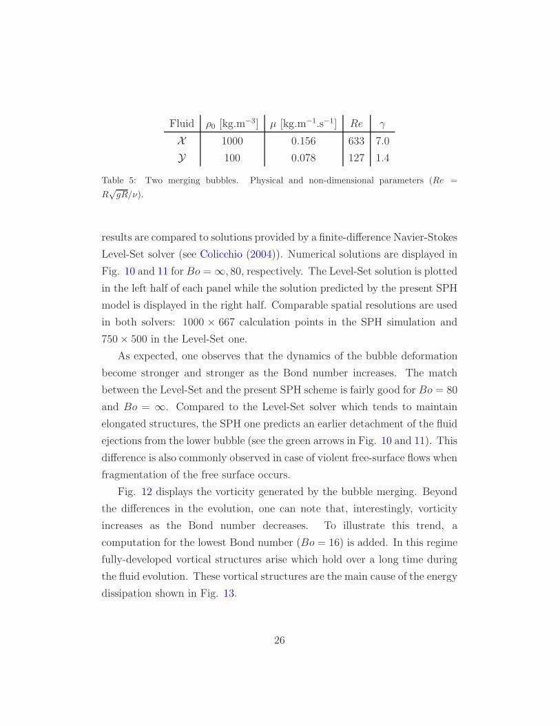
Fluid ρ0 [kg.m−3] µ [kg.m−1.s−1] Re γ

X 1000 0.156 633 7.0

Y 100 0.078 127 1.4

Table 5: Two merging bubbles. Physical and non-dimensional parameters (Re =

R√gR/ν).

results are compared to solutions provided by a finite-difference Navier-Stokes

Level-Set solver (see Colicchio (2004)). Numerical solutions are displayed in

Fig. 10 and 11 for Bo = ∞, 80, respectively. The Level-Set solution is plotted

in the left half of each panel while the solution predicted by the present SPH

model is displayed in the right half. Comparable spatial resolutions are used

in both solvers: 1000 × 667 calculation points in the SPH simulation and

750× 500 in the Level-Set one.

As expected, one observes that the dynamics of the bubble deformation

become stronger and stronger as the Bond number increases. The match

between the Level-Set and the present SPH scheme is fairly good for Bo = 80

and Bo = ∞. Compared to the Level-Set solver which tends to maintain

elongated structures, the SPH one predicts an earlier detachment of the fluid

ejections from the lower bubble (see the green arrows in Fig. 10 and 11). This

difference is also commonly observed in case of violent free-surface flows when

fragmentation of the free surface occurs.

Fig. 12 displays the vorticity generated by the bubble merging. Beyond

the differences in the evolution, one can note that, interestingly, vorticity

increases as the Bond number decreases. To illustrate this trend, a

computation for the lowest Bond number (Bo = 16) is added. In this regime

fully-developed vortical structures arise which hold over a long time during

the fluid evolution. These vortical structures are the main cause of the energy

dissipation shown in Fig. 13.

26

0.2 0.3 0.4 0.5 0.6 0.7 0.8

0.3

0.4

0.5

0.6

0.7

0.8

0.9

t (g/R)½ = 0.63y

x 0.2 0.3 0.4 0.5 0.6 0.7 0.8

0.3

0.4

0.5

0.6

0.7

0.8

0.9

t (g/R)½ = 1.27y

x

0.2 0.3 0.4 0.5 0.6 0.7 0.8

0.3

0.4

0.5

0.6

0.7

0.8

0.9

t (g/R)½ = 1.90y

x 0.2 0.3 0.4 0.5 0.6 0.7 0.8

0.3

0.4

0.5

0.6

0.7

0.8

0.9

t (g/R)½ = 2.53y

x

0.2 0.3 0.4 0.5 0.6 0.7 0.8

0.3

0.4

0.5

0.6

0.7

0.8

0.9

t (g/R)½ = 2.85y

x 0.2 0.3 0.4 0.5 0.6 0.7 0.8

0.3

0.4

0.5

0.6

0.7

0.8

0.9

t (g/R)½ =3.16y

x

Figure 10: Two merging bubbles for Bo = ∞. Left half of each panel: Navier-Stokes

Level-Set solver. Right half of each panel: present SPH model. Green arrows point out

the detachment of fluid ejections.

27

0.2 0.3 0.4 0.5 0.6 0.7 0.8

0.3

0.4

0.5

0.6

0.7

0.8

0.9

t (g/R)½ = 0.63y

x 0.2 0.3 0.4 0.5 0.6 0.7 0.8

0.3

0.4

0.5

0.6

0.7

0.8

0.9

t (g/R)½ = 1.27y

x

0.2 0.3 0.4 0.5 0.6 0.7 0.8

0.3

0.4

0.5

0.6

0.7

0.8

0.9

t (g/R)½ = 1.90y

x 0.2 0.3 0.4 0.5 0.6 0.7 0.8

0.3

0.4

0.5

0.6

0.7

0.8

0.9

t (g/R)½ = 2.53y

x

0.2 0.3 0.4 0.5 0.6 0.7 0.8

0.3

0.4

0.5

0.6

0.7

0.8

0.9

t (g/R)½ = 2.85y

x 0.2 0.3 0.4 0.5 0.6 0.7 0.8

0.3

0.4

0.5

0.6

0.7

0.8

0.9

t (g/R)½ = 3.16y

x

Figure 11: Two merging bubbles for Bo = 80. Left half of each panel: Navier-Stokes

Level-Set solver. Right half of each panel: present SPH model. The green arrow points

out the detachment of fluid ejections, occurring only with the SPH model.

28

Figure 12: Two merging bubbles. Vorticity field for different Bond numbers predicted by

the present SPH scheme.

0 1 2 3 4 5 6

-10.00

-8.00

-6.00

-4.00

-2.00

0.00

(EMEK - EMEK0) / (EMEK0 - EMEK f ) %

t(g/R)½

Bo = ∞

Bo = 80

Bo = 16

Figure 13: Two merging bubbles. Mechanical energy evolution of the present SPH scheme.

EMEKf is associated with the configuration in which the fluid Y lies above the fluid Xand both fluids are still.

29

4.3. Evolution of a set of bubbles

In the present section a demanding test case is performed by modeling

the gravity separation of a bubbly flow composed of bubbles of a light fluid

in and heavier one. It is similar to the bubble collision problem studied in

the previous section but with a larger number of bubbles. More specifically,

a set of 36 bubbles is considered. Bubbles are initially spread on a regular

6×6 lattice; they are then randomly shifted within ±50% of the inter-bubble

distance. Finally, their radii are randomly changed within ±50% as well, see

Fig. 14. The domain is sufficiently narrow to allow collisions between bubbles

X

Y

Y

L

HX

HY

Figure 14: Set of bubbles. Sketch of the initial configuration.

(L = HX = 26.6R). Above the bubbly flow, we set a layer of the lighter fluid

of height HY = 8.4R, which models the already separated part of the bubbly

flow towards which bubbles are migrating. The physical characteristics of

the two fluids, are summarized in Table 6. The chosen configuration tends to

mimic the fluid mixtures which sometimes occur in the offshore oil industry,

e.g. in oil-water separators, especially for densities which are close to the

one, as for water and oil. However, for numerical stability, the viscosity

of the heavier fluid is overestimated compared to water’s one. By analogy

between the MGF viscosity modeling, see eq. (22), and the artificial viscosity

30

Fluid ρ0 [kg.m−3] µ [kg.m−1.s−1]

X 1000 0.007

Y 800 0.0065

Table 6: Set of bubbles. Physical parameters.

of Monaghan (1992), one can found a relation between the physical viscosity

and the artificial viscosity parameter which ensures stable simulations.

The mean radius of bubbles is chosen equal to 1mm. This value is

a bit larger than the one found in actual separators of the offshore oil

industry (the biggest radii are close to 400 µm), but this allows us to

perform simulations of the water-oil separation process with less numerical

discretization constraints. The corresponding mean Reynolds number is 40.

Since the aim of the present investigation is not to study the interactions

between walls and bubbles, a free slip condition is imposed along the walls.

4.3.1. Influence of the Bond number

In the present section the influence of the surface tension on the separation

phenomenon is investigated. To do so, the Bond number is varied while

all the remaining parameters are kept constant. The Bond number based

on the minimal radius (i.e. 5× 10−4 m) ranges from 12.5 to 0.125, which

corresponds to σ ranging from 7.85× 10−4N.m−1 to 7.85× 10−2N.m−1. The

smoothing length is h = 10−4m.

By closely looking at Fig. 15, one can observe that the bubble rising

velocity is larger at low Bo numbers. This behavior is due to the fact that

the bubbles shape tends to remain circular. On the contrary, when the

surface tension is small, bubbles tend to stretch in the direction transverse

to their rising direction, i.e. they stretch horizontally. This change in shape

induces an increase in their drag. Actually, as already shown in Fig. 12,

the bubbles characterized by an elongated shape tend to drag a larger zone

31

Figure 15: Bubbly flow in a simplified closed oil-water separator. Density field at different

times for different Bond number.

of separated flow which slows them down. This effect is complemented by

the fact that, when two circular bubbles are merging, they result in a bigger

circular bubble with higher buoyancy and lower relative drag which tends to

rise faster towards the light fluid layer.

Regarding the bubble coalescence occurring during the simulations,

it is interesting to check whether this should physically occur in the

chosen configuration. To this purpose, one can the compare the

interaction time between two bubbles just before coalescence, namely tI =

32

√

π2 ρXCMd3/(48σ), to the characteristic drainage time tD = ρXVad2/(8σ)

(see Bonometti (2005); Kamp et al. (2001)). Here, CM is the added mass

coefficient predicted by the potential theory for two spheres of the same radius

in contact and aligned in the direction of the flow (specifically, CM = 0.803)

while Va is the velocity of approach of coalescing bubbles. The latter one

is calculated numerically by comparing inter-bubble distances at different

times. Using these definitions, we find that tI is always at least one order of

magnitude bigger than tD for all the considered Bond numbers. This means

that we are simulating a flow regime in which coalescence actually occur.

4.3.2. Quasi-infinite Bond number simulation

When simulating infinite Bond number flows, strong mixing occurs

between elements of the distinct fluids. To prevent mixing at the scale of

the fluid elements (that is, particles), a correction based on inter-particle

repulsive forces is introduced accordingly to the work of Grenier et al. (2009).

The coefficient used for this correction is ǫI = 10−3 (see Grenier et al. (2009)

for more details) while the smoothing length is h = 10−4m.

Figure 16 displays strong deformations of the bubble interfaces. The

bubble shape is much more affected by the surrounding flow than in the

previous simulation (see Fig. 15), even in comparison with the highest

Bond number (i.e. Bo = 12.5). This results in the formation of elongated

structures and in a much more complex mixing interface.

5. Conclusion

The multi-fluid scheme introduced in Grenier et al. (2009) is extended

and applied to study bubbly flows. A viscous formulation based on the

renormalization of the Morris et al. (1997) formula is introduced. This

formulation proves to be more accurate that the other formulations classically

used by SPH practitioners. This is illustrated on one- and two-fluid Poiseuille

flows, where a second-order convergence is obtained. A surface tension model

33

Figure 16: Bubbly flow in a simplified closed oil-water separator. Density field at different

times for a quasi-infinite Bond number.

is also proposed. This is based on a continuous surface stress approach and it

is also carefully validated on classical bubble oscillation test cases. Linear to

second-order convergence is obtained on these test cases. Parasitic currents

are also investigated.

In the second part, bubbly flows of increasing complexity are studied.

First, the buoyant rise of a single bubble at low Bond number is investigated.

Convergence is obtained to a reference analytical solution. Then, the collision

of two bubbles is examined in detail. The bubble merging process is compared

to a Level-set Navier-Stokes solver solution for different Bond numbers,

showing comparable results except for the fragmentation of elongated

structures. The vorticity field induced by this process is also inspected.

Finally, the gravity separation of a bubbly oil-water flow is studied. The

34

proposed method enables us to accurately simulate such flows even at low

resolution, since the Lagrangian nature of the SPH method allows preserving

a perfectly-sharp interface during the evolution.

Further work will concern more realistic validations with comparisons

between tree-dimensional simulations and experiments.

Acknowledgements

The research leading to these results has received funding from the

European Community’s Seventh Framework Programme (FP7/2007-2013)

under grant agreement n.225967 “NextMuSE”.

This work has been also partially funded by the Centre of Excellence

CeSOS/AMOS, NTNU, Norway.

A. Equation of state

The continuum system (1) corresponds to the compressible

Navier-Stokes equations with an isentropic equation of state (EOS)

as a closure law. This is essentially a hyperbolic system which

propagates information at a characteristic velocity |u| + c, where c

is the speed of sound. For an easy and efficient parallelization, the

time forwarding scheme must be explicit and, then, its stability is

restricted by the Courant-Friedrichs-Lewy condition based on the

aforementioned characteristic velocity.

For real compressible fluids in subsonic flows (i.e., c is real

and |u| < c), this condition leads to huge computational costs. A

possible solution is to use a weakly-compressible approach. This

consists in the following bound on the density variation, ∆ρ:

∆ρ

ρ0≪ 1 (25)

35

To link the above condition to the speed of sound, we consider the

isotherm compressibility of a general EOS:

χT =1

ρ

(

∂ρ

∂p

)

T

. (26)

Approximating this later definition through small variations,

equation (25) can be rewritten as follows:

χT∆p ≪ 1 . (27)

This later expression underlines that the artificial compressibility

of the fluid must be compatible with the magnitude of the expected

pressure variations inside the flow.

For the chosen EOS (Tait’s equation), this isotherm

compressibility is equal to:

χT =1

ρc20

(

ρ

ρ0

)γ−1

≃ 1

ρ0c20(28)

where the last term has been approximated by using the initial

reference density ρ0.

Most of SPH practitioner are interested in flows in which

the highest pressure variations are of magnitude of the dynamic

pressure ρ0|u|2. With this assumption and Tait’s EOS, the relation

(27) gives:|u|2c20

≪ 1 (29)

which is the classical assumption for SPH simulations.

If we are interested in gravity-based flows, highest pressure

variations can be of magnitude of the hydrostatic pressure ρ0gH

(where H is the reference water depth). With this assumption and

Tait’s EOS, the relation (27) gives:

gH

c20≪ 1. (30)

36

If we are interested in surface tension-driven flows, the pressure

variations are of magnitude of the Laplace law pressure 2σ/R

(where R is the characteristic radius of curvature). This leads

to:2σ

ρ0c20R

≪ 1. (31)

The conditions (29), (30) and ((31) are used to estimate ‘a

priori ’ the speed of sound of the fluid.

References

Abdulkadir, M., Hernandez-Perez, V., 2010. The effect of mixture velocity

and droplet diameter on oil-water separator using computational fluid

dynamics (cfd). World Academy of Science, Engineering and Technology

37, 35–43.

Adami, S., Hu, X., Adams, N., 2010. A new surface-tension formulation for

multi-phase sph using a reproducing divergence approximation. Journal of

Computational Physics 229, 5011 – 5021.

Antuono, M., Colagrossi, A., Marrone, S., Lugni, C., 2011. Propagation

of gravity waves through an SPH scheme with numerical diffusive terms.

Computer Physics Communications 182, 866 – 877.

Bonometti, T., 2005. Developpement d’une methode de simulation

d’ecoulements a bulles et a gouttes. Ph.D. thesis. Institut National

Polytechnique de Toulouse, France. Ph.D. thesis (in French).

Brackbill, J.U., Kothe, D.B., Zemach, C., 1992. A continuum method for

modeling surface tension. Journal of Computational Physics 100, 335–354.

37

Bunner, B., Tryggvason, G., 2003. Effect of bubble deformation on the

properties of bubbly flows. Journal of Fluid Mechanics 495, 77–118.

Colicchio, G., 2004. Violent disturbance and fragmentation of free surfaces.

Ph.D. thesis. University of Southampton.

Cueille, P.V., 2005. Modelisation par SPH des phenomenes de diffusion

presents dans un ecoulement fluide. Ph.D. thesis. INSA Toulouse. Ph.D.

thesis (in French).

Das, A., Das, P., 2009. Bubble evolution through submerged orifice

using smoothed particle hydrodynamics: Basic formulation and model

validation. Chemical Engineering Science 64, 2281 – 2290.

Das, A.K., Das, P.K., 2011. Incorporation of diffuse interface in smoothed

particle hydrodynamics: Implementation of the scheme and case studies.

International Journal for Numerical Methods in Fluids 67, 671–699.

Das, A.K., Das, P.K., 2013. Bubble evolution and necking at a submerged

orifice for the complete range of orifice tilt. AIChE Journal 59, 630–642.

De Leffe, M., Le Touze, D., Alessandrini, B., 2011. A modified no-

slip condition in weakly-compressible SPH, in: 6th SPHERIC workshop,

Hamburg, Germany.

Delorme, L., Colagrossi, A., Souto-Iglesias, A., Zamora-Rodrguez, R., Bota-

Vera, E., 2009. A set of canonical problems in sloshing, part i: Pressure

field in forced rollcomparison between experimental results and sph. Ocean

Engineering 36, 168 – 178.

Dijkhuizen, W., Roghair, I., Annaland, M.V.S., Kuipers, J., 2010. Dns of gas

bubbles behaviour using an improved 3d front tracking modeldrag force on

isolated bubbles and comparison with experiments. Chemical Engineering

Science 65, 1415 – 1426.

38

Duret, B., Luret, G., Reveillon, J., Menard, T., Berlemont, A., Demoulin, F.,

2012. Dns analysis of turbulent mixing in two-phase flows. International

Journal of Multiphase Flow 40, 93 – 105.

Flekkøy, E., Coveney, P., de Fabritiis, G., 2000. Foundations of dissipative

particle dynamics. Physical Review E 62, Issue 2, 2140-2157.

Francois, M.M., Cummins, S.J., Dendy, E.D., Kothe, D.B., Sicilian,

J.M., Williams, M.W., 2006. A balanced-force algorithm for continuous

and sharp interfacial surface tension models within a volume tracking

framework. Journal of Computational Physics 213, 141 – 173.

Frising, T., Nok, C., Dalmazzone, C., 2006. The liquid/liquid sedimentation

process: From droplet coalescence to technologically enhanced water/oil

emulsion gravity separators: A review. Journal of Dispersion Science and

Technology 27, 1035–1057.

Grenier, N., Antuono, M., Colagrossi, A., Touze, D.L., Alessandrini, B.,

2009. An hamiltonian interface SPH formulation for multi-fluid and free

surface flows. Journal of Computational Physics 228, 8380 – 8393.

Hu, X., Adams, N., 2006. A multi-phase SPH method for macroscopic and

mesoscopic flows. Journal of Computational Physics 213, 844 – 861.

Kamp, A., Chesters, A., Colin, C., Fabre, J., 2001. Bubble coalescence in

turbulent flows: A mechanistic model for turbulence-induced coalescence

applied to microgravity bubbly pipe flow. International Journal of

Multiphase Flow 27-8, 1363–1396.

Khayyer, A., Gotoh, H., 2012. A consistent particle method for simulation

of multiphase flows with high density ratios, in: 7th SPHERIC workshop,

Prato, Italy.

39

Lafaurie, B., Nardone, C., Scardovelli, R., Zaleski, S., Zanetti, G., 1994.

Modelling merging and fragmentation in multiphase flows with surfer.

Journal of Computational Physics 113, Issue 1, 134–147.

Laleh, A.P., Svrcek, W.Y., Monnery, W.D., 2012. Design and cfd studies

of multiphase separatorsa review. The Canadian Journal of Chemical

Engineering 90, 1547–1561.

Lamb, H., 1932. Hydrodynamics. Dover, New York.

Landrini, M., Colagrossi, A., Greco, M., Tulin, M., 2012. The fluid mechanics

of splashing bow waves on ships: A hybrid bemsph analysis. Ocean

Engineering 53, 111 – 127.

Leduc, J., Leboeuf, F., Lance, M., Parkinson, E., Marongiu, J.C., 2010. A

SPH-ALE method to model multiphase flow with surface tension, in: 7th

International Conference on Multiphase Flow, Tampa, United States of

America.

Macia, F., Antuono, M., Gonzalez, L.M., Colagrossi, A., 2011. Theoretical

analysis of the no-slip boundary condition enforcement in SPH methods.

Progress of Theoretical Physics 125, 1091–1121.

Marrone, S., Colagrossi, A., Antuono, M., Colicchio, G., Graziani, G.,

2013. An accurate sph modeling of viscous flows around bodies at low

and moderate reynolds numbers. accepted for publication on Journal of

Computational Physics .

Monaghan, J., 2012. Smoothed particle hydrodynamics and its diverse

applications. Annual Review of Fluid Mechanics 44, 323–346.

Monaghan, J.J., 1992. Smoothed particle hydrodynamics. Annual review of

Astronomy and Astrophysics 30, 543–574.

40

Monaghan, J.J., 2000. Sph without a tensile instability. Journal of

Computational Physics 159, 290–311.

Monaghan, J.J., Gingold, R.A., 1983. Shock simulation by the particle

method sph. Journal of Computational Physics 52, 374–389.

Morris, J.P., 2000. Simulating surface tension with smoothed particle

hydrodynamics. International Journal of Numerical Methods in Fluids

33, 333–353.

Morris, J.P., Fox, P.J., Zhu, Y., 1997. Modeling low reynolds number

incompressible flows using sph. Journal of Computational Physics 136,

214 – 226.

Popinet, S., 2009. An accurate adaptive solver for surface-tension-driven

interfacial flows. Journal of Computational Physics 228, 5838 – 5866.

Popinet, S., Zaleski, S., 1999. A front-tracking algorithm for accurate

representation of surface tension. International Journal for Numerical

Methods in Fluids 30, 775–793.

Price, D.J., 2008. Modelling discontinuities and kelvinhelmholtz instabilities

in sph. Journal of Computational Physics 227, 10040 – 10057.

Prosperetti, A., 1980. Normal-mode analysis ofr the oscillations of a viscous

liquid drop in a immiscible liquid. Journal de Mcanique 19, 149–182.

Renardy, Y., Renardy, M., 2002. PROST: A parabolic reconstruction of

surface tension for the volume-of-fluid method. Journal of Computational

Physics 183, 400–421.

Slot, J., Van Campen, L., Hoeijmakers, H., Mudde, R., 2011. In-line oil-water

separation in swirling flow, in: 8th International Conference on CFD in

Oil & Gas, Metallurgical and Process Industries, Trondheim, Norway.

41

Swegle, J.W., Hicks, D.L., Attaway, S.W., 1995. Smoothed particle

hydrodynamics stability analysis. Journal of Computational Physics 116,

123–134.

Szewc, K., Pozorski, J., Minier, J.P., 2013. Simulations of single bubbles

rising through viscous liquids using smoothed particle hydrodynamics.

International Journal of Multiphase Flow 50, 98 – 105.

Tartakovsky, A.M., Meakin, P., 2005. A smoothed particle hydrodynamics

model for miscible flow in three-dimensional fractures and the two-

dimensional rayleightaylor instability. Journal of Computational Physics

207, 610 – 624.

Torres, D.J., Brackbill, J.U., 2000. The Point-Set Method: Front-Tracking

without connectivity. Journal of Computational Physics 165, 620 – 644.

Tryggvason, G., Lu, J., Biswas, S., Esmaeeli, A., 2009. Studies of

bubbly channel flows by direct numerical simulations, in: Deville, M.,

L, T.H., Sagaut, P. (Eds.), Turbulence and Interactions. Springer Berlin

/ Heidelberg. volume 105 of Notes on Numerical Fluid Mechanics and

Multidisciplinary Design, pp. 93–111.

Vincent, S., Larocque, J., Lacanette, D., Toutant, A., Lubin, P., Sagaut, P.,

2008. Numerical simulation of phase separation and a priori two-phase les

filtering. Computers & Fluids 37, 898 – 906.

Violeau, D., Buvat, C., Abed-Meraim, K., de Nanteuil, E., 2007. Numerical

modelling of boom and oil spill with sph. Coastal Engineering 54, 895 –

913.

Zhang, D.Z., Prosperetti, A., 1994. Averaged equations for inviscid disperse

two-phase flow. Journal of Fluid Mechanics 267, 185–219.

42