Visco-potential free-surface flows and long wave modelling

Visco-potential free-surface flows and long

wave modelling

Denys Dutykh a,∗aCMLA, ENS Cachan, CNRS, PRES UniverSud, 61 Av. President Wilson,

F-94230 Cachan, France 1

Abstract

In a previous study [DD07b] we presented a novel visco-potential free surface flowsformulation. The governing equations contain local and nonlocal dissipative terms.From physical point of view, local dissipation terms come from molecular viscos-ity but in practical computations, rather eddy viscosity should be used. On theother hand, nonlocal dissipative term represents a correction due to the presenceof a bottom boundary layer. Using the standard procedure of Boussinesq equationsderivation, we come to nonlocal long wave equations. In this article we analysedispersion relation properties of proposed models. The effect of nonlocal term onsolitary and linear progressive waves attenuation is investigated. Finally, we presentsome computations with viscous Boussinesq equations solved by a Fourier typespectral method.

Key words: free-surface flows, viscous damping, long wave models, Boussinesqequations, dissipative Korteweg-de Vries equation, bottom boundary layerPACS: 47.35.Bb, 47.35.Fg, 47.10.ad

1 Introduction

Even though the irrotational theory of free-surface flows can predict success-fully many observed wave phenomena, viscous effects cannot be neglectedunder certain circumstances. Indeed the question of dissipation in potentialflows of fluid with a free surface is an important one. As stated by [LH92],

∗ Corresponding author.Email address: [email protected] (Denys Dutykh).

1 Now at LAMA, University of Savoie, CNRS, Campus Scientifique, 73376 LeBourget-du-Lac Cedex, France

Preprint submitted to Eur. J. Mech. B/Fluids 13th November 2008

hal-0

0270

926,

ver

sion

4 -

13 N

ov 2

008

it would be convenient to have equations and boundary conditions of com-parable simplicity as for undamped free-surface flows. The peculiarity herelies in the fact that the viscous term in the Navier–Stokes (NS) equations isidentically equal to zero for a velocity deriving from a potential. There is alsoa problem with boundary conditions. It is well known that the usual non-slipcondition on the solid boundaries does not allow to simulate free surface flowsin a finite container. Hence, some further modifications are required to permitthe free surface particles to slide along the solid boundary. These difficultieswere overcome in our recent work [DD07b] and [DDZ08].

The effects of viscosity on gravity waves have been addressed since the endof the nineteenth century in the context of the linearized Navier–Stokes (NS)equations. It is well-known that Lamb [Lam32] studied this question in thecase of oscillatory waves on deep water. What is less known is that Boussinesqstudied this effect as well [Bou95]. In this particular case they both showedthat

dα

dt= −2νk2α, (1)

where α denotes the wave amplitude, ν the kinematic viscosity of the fluidand k = 2π/ℓ the wavenumber of the decaying wave. Here ℓ stands for thewavelength. This equation leads to the classical law for viscous decay, namely

α(t) = α0e−2νk2t. (2)

Let us consider a simple numerical application with g = 9.8 m/s2, ℓ = 3 mand molecular viscosity ν = 10−6 m2/s. According to the formula (2), thiswave will take t0 ≈ 8 × 104 s or about one day before losing one half of itsamplitude. This wave will attain velocity

cp =

√g

k≈ 2.16 m/s

and travel the distance equal to L = cp · t0 ≈ 170 km. This estimation isexaggerated since the classical result of Boussinesq and Lamb does not takeinto account energy dissipation in the bottom boundary layer. We will discussthe question of linear progressive waves attenuation in Section 5. Anotherpoint is that the molecular viscosity ν should be replaced by eddy viscosityνt which is more appropriate in most practical situations (see Remark 6 formore details).

The importance of viscous effects for water waves has been observed in variousexperimental studies. For example, in [ZG71] one can read

. . . However, the amplitude disagrees somewhat, and we suppose that thismight be due to the viscous dissipation. . .

[Wu81] also mentions this drawback of the classical water wave theory:

2

hal-0

0270

926,

ver

sion

4 -

13 N

ov 2

008

. . . the peak amplitudes observed in the experiments are slightly smallerthan those predicted by the theory. This discrepancy can be ascribed to theneglect of the viscous effects in the theory. . .

Another example is the conclusion of [BPS81]:

. . . it was found that the inclusion of a dissipative term was much more im-portant than the inclusion of the nonlinear term, although the inclusion ofthe nonlinear term was undoubtedly beneficial in describing the observa-tions. . .

Another source of dissipation is due to bottom friction. An accurate computa-tion of the bottom shear stress ~τ is crucial for calculating sediment transportfluxes. Consequently, the predicted morphological changes will greatly dependon the chosen shear stress model. Traditionally, this quantity is modelled bya Chezy-type law

~τ |z=−h = Cfρ|~uh|~uh,where ~uh = ~u(x, y,−h, t) is the fluid velocity at the bottom, Cf is the frictioncoefficient and ρ is the fluid density. Two other often used laws can be foundin [DD07a, Section 4.3], for example. One problem with this model is that ~τand ~uh are in phase. It is well known [LSVO06] that in the case of a laminarboundary layer, the bottom stress ~τ |z=−h is π

4out of phase with respect to the

bottom velocity.

Water wave energy can be dissipated by different physical mechanisms. Theresearch community agrees at least on one point: the molecular viscosity isunimportant. Now let us discuss more debatable statements. For example if wetake a tsunami wave and estimate its Reynolds number, we find Re ≈ 106. So,the flow is clearly turbulent and in practice it can be modelled by various eddyviscosity models. On the other hand, in laboratory experiments the Reynoldsnumber is much more moderate and sometimes we can neglect this effect.When nonbreaking waves feel the bottom, the most efficient mechanism ofenergy dissipation is the bottom boundary layer. This is the focus of our paper.We briefly discuss the free surface boundary layer and explain why we do nottake it into account in this study. Finally, the most important (and the mostchallenging) mechanism of energy dissipation is wave breaking. This process isextremely difficult from the mathematical but also the physical and numericalpoints of view since we have to deal with multivalued functions, topologicalchanges in the flow and complex turbulent mixing processes. Nowadays thepractitioners can only be happy to model roughly this process by adding ad-hoc dissipative terms when the wave becomes steep enough.

In this work we keep the features of undamped free-surface flows while addingdissipative effects. The classical theory of viscous potential flows is based onpressure and boundary conditions corrections [JW04] due to the presence of

3

hal-0

0270

926,

ver

sion

4 -

13 N

ov 2

008

viscous stresses. We present here another approach.

Currently, potential flows with ad-hoc dissipative terms are used for examplein direct numerical simulations of weak turbulence of gravity waves [DKZ03,DKZ04, ZKPD05]. There have also been several attempts to introduce dis-sipative effects into long wave modelling [Mei94, DD07a, CG07, Kha97]. Wewould like to underline that the last paper [Kha97] contains also a nonlocaldissipative term in time.

The present work is a direct continuation of the recent studies [DDZ08, DD07b].In [DDZ08] the authors considered periodic waves in infinite depth and deriva-tion was done in two-dimensional (2D) case, while in [DD07b] we removedthese two hypotheses and all the computations are done in 3D. This point isimportant since the vorticity structure is more complicated in 3D. In otherwords we considered a general wavetrain on the free surface of a fluid layer offinite depth. As a result we obtained a formulation which contains a nonlocalterm in the bottom kinematic condition. Later we discovered that the nonlocalterm in exactly the same form was derived in [LO04]. The inclusion of thisterm is natural since it represents the correction to potential flow due to thepresence of a boundary layer. Moreover, this term is predominant since itsmagnitude scales with O(

√ν), while other terms in the free-surface boundary

conditions are of order O(ν). The importance of this effect was pointed out inthe classical literature on the subject [Lig78]:

. . . Bottom friction is the most important wherever the water depth is sub-stantially less than a wavelength so that the waves induce significant hor-izontal motions near the bottom; the associated energy dissipation takesplace in a boundary layer between them and the solid bottom. . .

This quotation means that this type of phenomenon is particularly importantfor shallow water waves like tsunamis, for example [DD06, Dut07]. Here wepresent several numerical computations based on the newly derived governingequations and analyse dispersion relation properties.

We would like to mention here a paper of N. Sugimoto [Sug91]. The authorconsidered initial-value problems for the Burgers equation with the inclusionof a hereditary integral known as the fractional derivative of order 1

2. The

form of this term was justified in previous works [Sug89, Sug90]. Note, thatfrom fractional calculus point of view our nonlocal term (6) is also a half-orderintegral.

Other researchers have obtained nonlocal corrections but they differ from ours[KM75]. This discrepancy can be explained by a different scaling chosen byKakutani & Matsuuchi in the boundary layer. Consequently, their governingequations contain a nonlocal term in space. The performance of the presentnonlocal term (6) was studied in [LSVO06]. The authors carried out in a wave

4

hal-0

0270

926,

ver

sion

4 -

13 N

ov 2

008

tank a set of experiments, analyzing the damping and shoaling of solitarywaves. It is shown that the viscous damping due to the bottom boundarylayer is well represented by the nonlocal term. Their numerical results fit wellwith the experiments. The model not only properly predicts the wave heightat a given point but also provides a good representation of the changes onthe shape and celerity of the soliton. We can conclude that the experimentalstudy by P. Liu et al. [LSVO06] validates this theory.

The present article is organized as follows. In Section 2 we estimate the rate ofviscous dissipation in different regions of the fluid domain. Then, we presentbasic ideas of derivation and come up with visco-potential free-surface flowsformulation. At the end of Section 3 we give corresponding long wave models:nonlocal Boussinesq and KdV equations. Section 4 is completely devoted tothe analysis of linear dispersion relation of complete and long wave modelsintroduced in previous section. Last two sections deal with linear progressiveand solitary waves attenuation respectively. Finally, the paper is ended bysome conclusions and perspectives.

2 Anatomy of dissipation

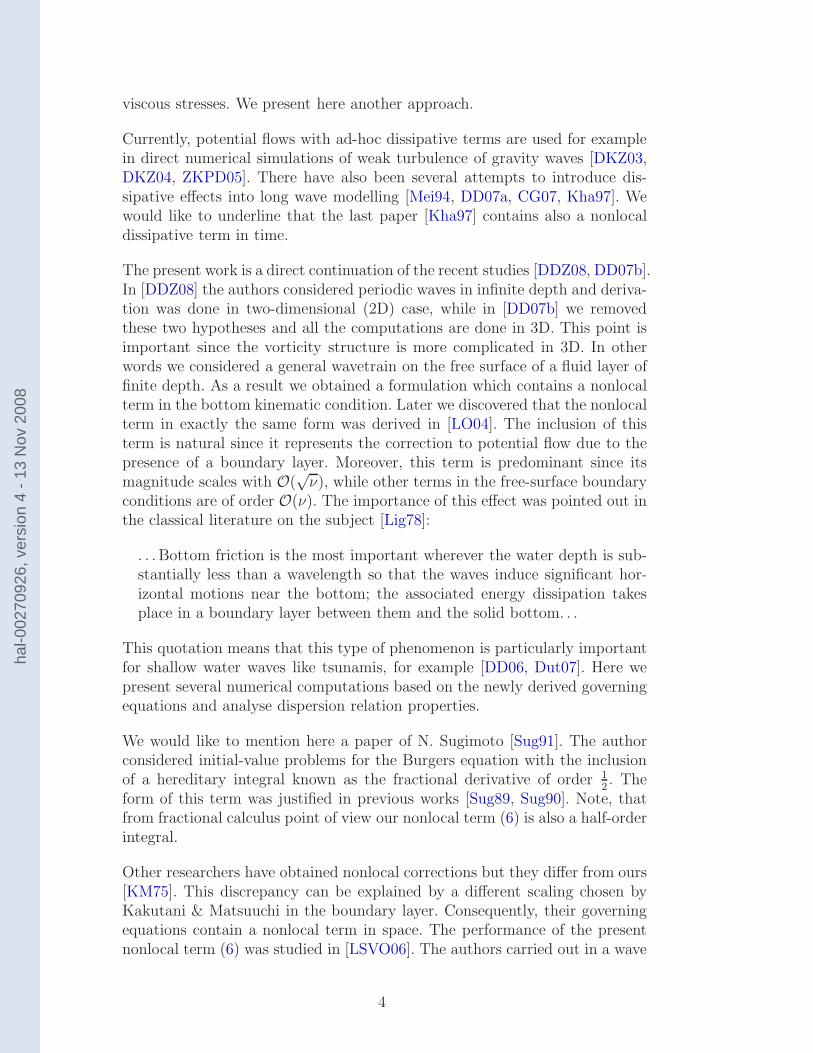
In this section we briefly discuss the contribution of different flow regions intowater wave energy dissipation. We conventionally [Mei94] divide the flow intothree regions illustrated on Figure 1. On this figure Sf and Sb stand for freesurface and bottom respectively. Then, Ri, Rf and Rb denote the interiorregion, free surface and bottom boundary layers.

O ~x

z

Sf

Sb

Rf

Rb

Ri

Figure 1. Conventional partition of the flow region into interior region and freesurface, bottom boundary layers.

In order to make some estimates we introduce the notation which will be usedin this section: µ is the dynamic viscosity, δ = O(

õ) is the boundary layer

5

hal-0

0270

926,

ver

sion

4 -

13 N

ov 2

008

thickness, t0 is the characteristic time, a0 is the characteristic wave amplitudeand ℓ is the wavelength.

We assume that the flow is governed by the incompressible Navier-Stokesequations:

∇ · ~u=0,∂~u

∂t+ ~u · ∇~u+

1

ρ∇p=~g +

1

ρ∇ · τ ,

where τ is the viscous stress tensor

τij = 2µεij, εij =1

2

(∂ui∂xj

+∂uj∂xi

)

.

We multiply the second equation by ~u and integrate over the domain Ω withboundary ∂Ω to get the following energy balance equation:

1

2

∫

Ω

∂

∂t

(

ρ|~u|2)

dΩ +1

2

∫

∂Ω

ρ|~u|2~u · ~n dσ =

=∫

∂Ω

(

−pI + τ)

~n · ~u dσ +∫

Ω

ρ~g · ~u dΩ − 1

2µ

∫

Ω

τ : τ dΩ

︸ ︷︷ ︸

T

.

In this identity each term has a precise physical meaning. The left-hand sideis the total rate of energy change in Ω. The second term is the flux of energyacross the boundary. On the right-hand side, the first integral represents therate of work by surface stresses acting on the boundary. The second integralis the rate of work done by the gravity force throughout the volume, and thethird integral T is the rate of viscous dissipation. We focus our attention onthe last term T . We estimate the order of magnitude of the rate of dissipationin various regions of the fluid.

We start by the interior regionRi. Outside the boundary layers, it is reasonableto expect that the rate of strain is dominated by the irrotational part of thevelocity whose scale is a0

t0and the length scale is the wavelength ℓ. The energy

dissipation rate is then

O(

TRi

)

∼ 1

µ

(

µa

t0ℓ

)2

· ℓ3 = µ(a

t0

)2

ℓ ∼ O(µ) .

Inside the bottom boundary layer the normal gradient of the solenoidal part

6

hal-0

0270

926,

ver

sion

4 -

13 N

ov 2

008

of ~u dominates the strain rate, so that

O(

TRb

)

∼ 1

µ

(

µa

t0δ

)2

· δℓ2 =µ

δ

(aℓ

t0

)2

∼ O(µ1

2 ) .

A free surface boundary layer also exists. Its importance depends on the freesurface conditions. Consider first the classical case of a clean surface. Thestress is mainly controlled by the potential velocity field which is of the sameorder as in the main body of the fluid. Because of the small volume O(δℓ2)the rate of dissipation in the free surface boundary layer is only

O(

TRf

)

∼ 1

µ

(

µa

t0ℓ

)2

· δℓ2 = µδ(a

t0

)2

∼ O(µ3

2 ) .

From the physical point of view it is weaker, since only the zero shear stresscondition on the free surface is required.

Another extreme case is when the free surface is heavily contaminated, forexample, by oil slicks. The stress in the free surface boundary layer can thenbe as great as in the boundary layer near a solid wall. In the present study wedo not treat such extreme situations and the surface contamination is assumedto be absent.

The previous scalings suggest the following diagram which represents the hi-erarchy of dissipative terms:

O(

µ1

2

)

︸ ︷︷ ︸

Rb

→ O(µ)︸ ︷︷ ︸

Ri

→ O(

µ3

2

)

︸ ︷︷ ︸

Rf

→ . . .

It is clear that the largest energy dissipation takes place inside the bottomboundary layer. We take into account only two first phenomena from thisdiagram. Consequently, all dissipative terms of order O(µ

3

2 ) and higher willbe neglected.

Remark 1 In laboratory experiments, surface waves are confined by side wallsas well. The rate of attenuation due to the side-wall boundary layers was com-puted in [ML73]. For simplicity, in the present study we consider an unboundedin horizontal coordinates domain (see Figure 1).

7

hal-0

0270

926,

ver

sion

4 -

13 N

ov 2

008

3 Derivation

Consider the linearized 3D incompressible NS equations describing free-surfaceflows in a fluid layer of uniform depth h:

∂~v

∂t= −1

ρ∇p+ ν∆~v + ~g, ∇ · ~v = 0, (3)

with ~v the velocity vector, p the pressure, ρ the fluid density and ~g the acceler-ation due to gravity. We represent ~v = (u, v, w) in the form of the Helmholtz–Leray decomposition:

~v = ∇φ+ ∇× ~ψ, ~ψ = (ψ1, ψ2, ψ3). (4)

After substitution of the decomposition (4) into (3), one notices that the

equations are verified provided that the functions φ and ~ψ satisfy the followingequations:

∆φ = 0, φt +p− p0

ρ+ gz = 0,

∂ ~ψ

∂t= ν∆~ψ.

Next we discuss the boundary conditions. We assume that the velocity fieldsatisfies the conventional no-slip condition at the bottom ~v|z=−h = ~0, while atthe free surface we have the usual kinematic condition, which can be statedas

ηt + ~v · ∇η = w.

After linearization it becomes simply ηt = w.

Dynamic condition states that the forces must be equal on both sides of thefree surface:

[~σ · ~n] ≡ −(p− p0)~n+ τ · ~n = 0 at z = η(x, t) ,

where ~σ is the stress tensor, [f ] denotes the jump of a function f across thefree surface, ~n is the normal to the free surface and τ the viscous part of thestress tensor ~σ.

The basic idea consists in expressing the vortical part of the velocity field∇ × ~ψ in terms of the velocity potential φ and the free surface elevation ηusing differential or pseudodifferential operators. In this section we just showfinal results while the details of computation can be found in [DD07b, Dut07].

Let us begin by the free-surface kinematic condition

∂η

∂t= w ≡ ∂φ

∂z+∂ψ2

∂x− ∂ψ1

∂y, z = 0.

8

hal-0

0270

926,

ver

sion

4 -

13 N

ov 2

008

Using the absence of tangential stresses on the free surface, one can replacethe rotational part in the kinematic boundary condition:

ηt = φz + 2ν∆η.

In order to account for the presence of viscous stresses, we have to modifythe dynamic free-surface condition as well. This is done using the balance ofnormal stresses at the free surface:

σzz = 0 at z = 0 ⇒ p− p0 = 2ρν∂w

∂z≡ 2ρν

(∂2φ

∂z2+∂2ψ2

∂x∂z− ∂2ψ1

∂y∂z

)

.

In [DD07b] it is shown that ∂2ψ2

∂x∂z− ∂2ψ1

∂y∂z= O(ν

1

2 ), so Bernoulli’s equationbecomes

φt + gη + 2νφzz + O(ν3

2 ) = 0. (5)

Since we only consider weak dissipation (ν ∼ 10−6 − 10−3 m2/s), we neglectterms of order o(ν).

The second step in our derivation consists in introducing a boundary layercorrection at the bottom. In the present study we assume the boundary layerto be laminar. The question of turbulent boundary layer was investigated in[Liu06]. Hence, the bottom boundary condition becomes

∂φ

∂z

∣∣∣∣∣z=−h

=

√ν

π

t∫

0

∇2~xφ0|z=−h√t− τ

dτ = −√ν

π

t∫

0

φ0zz|z=−h√t− τ

dτ. (6)

One recognizes on the right-hand side a half-order integral operator. The lastequation shows that the effect of the diffusion process in the boundary layeris not instantaneous. The result is cumulative and it is weighted by (t− τ)−

1

2

in favour of the present time.

Summarizing the developments made above and generalizing our equationsby including nonlinear terms, we obtain a set of viscous potential free-surfaceflow equations:

∆φ= 0, (~x, z) ∈ Ω = R2 × [−h, η] (7)

ηt + ∇η · ∇φ=φz + 2ν∆η, z = η (8)

φt +1

2|∇φ|2 + gη=−2νφzz, z = η (9)

φz =−√ν

π

t∫

0

φzz√t− τ

dτ, z = −h. (10)

At the present stage, the addition of nonlinear terms is rather a conjecture.However, a recent study by Liu et al. [LPC07] suggests that this conjecture

9

hal-0

0270

926,

ver

sion

4 -

13 N

ov 2

008

is rather true. The authors investigated the importance of nonlinearity inthe bottom boundary layer for a solitary wave solution. They came to theconclusion that “the nonlinear effects are not very significant”.

Using this weakly damped potential flow formulation and described in previousworks procedure [DD07a, Section 4] of Boussinesq equations derivation, onecan derive the following system of equations with horizontal velocity ~uθ definedat the depth zθ = −θh, 0 ≤ θ ≤ 1:

ηt+∇· ((h+ η)~uθ)+h3

(

θ2

2− θ +

1

3

)

∇2(∇·~uθ) = 2ν∆η+

√ν

π

t∫

0

∇ · ~uθ√t− τ

dτ,

(11)

~uθt +1

2∇|~uθ|2 + g∇η − h2θ

(

1 − θ

2

)

∇(∇ · ~uθt) = 2ν∆~uθ. (12)

For simplicity, in this study we present governing equations only on the flatbottom, but generalization can be done for general bathymetry. Khabakhpa-shev [Kha87], Liu & Orfila [LO04] also derived a similar set of Boussinesqequations in terms of depth-averaged velocity. Our equations (11) – (12) havelocal dissipative terms in addition and they are formulated in terms of the ve-locity variable defined at arbitrary water level that is beneficial for dispersionrelation properties.

3.1 Total energy decay in visco-potential flow

Let us consider a fluid layer infinite in horizontal coordinates ~x = (x, y),bounded below by the flat bottom z = −h and above by the free surface.Total energy of water waves is given by the following formula:

E =∫∫

R2

η∫

−h

1

2|∇φ|2dzd~x+

g

2

∫∫

R2

η2d~x.

We would like to mention here that Zakharov showed [Zak68] this expressionto be the Hamiltonian for classical water wave problem with suitable choiceof canonical variables: η and ψ := φ(~x, z = η, t).

In this section we are interested in the evolution of the total energy E withtime. This question is investigated by computing the derivative dE

dtwith respect

to time t. Obviously, when one considers the classical potential free surfaceflow formulation [Lam32], we have dE

dt≡ 0, since no dissipation is introduced

into the governing equations. We performed the computation of dEdt

in theframework of the visco-potential formulation and give here the final result:

10

hal-0

0270

926,

ver

sion

4 -

13 N

ov 2

008

dEdt

=

√ν

π

∫∫

R2

φt|z=−h

t∫

0

φzz|z=−h√t− τ

dτd~x+ 2ν∫∫

R2

∂t(∇φ|z=η · ∇η) d~x.

In this identity, the first term on the right hand side comes from the boundarylayer and is predominant in the energy decay since its magnitude scales withO(

√ν). The second term has its origins in free surface boundary conditions.

Its magnitude is O(ν), thus it has less important impact on the energy balance.This topic will be investigated further in future studies.

3.2 Dissipative KdV equation

In this section we derive a viscous Korteweg-de Vries (KdV) equation from justobtained Boussinesq equations (11), (12). Since KdV-type equations modelonly unidirectional wave propagation, our attention is naturally restricted to1D case. In order to perform asymptotic computations, all the equations haveto be switched to nondimensional variables as it is explained in [DD07a, Sec-tion 2]. We find the velocity variable u in this form:

uθ = η + εP + µ2Q+ . . .

where ε, µ are nonlinearity and dispersion parameters respectively (see [DD07a]for their definition), P and Q are unknown at the present moment. Using themethods similar to those used in [DD07a, Section 6.1], one can easily showthat

P = −1

4η2, Q =

(

θ − 1

6− θ2

2

)

ηxx.

This result immediately yields the following asymptotic representation of thevelocity field

uθ = η − 1

4εη2 + µ2

(

θ − 1

6− θ2

2

)

ηxx + . . . (13)

Substituting the last formula (13) into equation (11) and switching again todimensional variables, one obtains this viscous KdV-type equation:

ηt +

√g

h

(

(h+3

2η)ηx +

1

6h3ηxxx −

√ν

π

t∫

0

ηx√t− τ

dτ)

= 2νηxx. (14)

This equation will be used in Section 5 to study the damping of linear progres-sive waves. Integral damping terms are reasonably well known in the context ofKdV type equations. Various nonlocal corrections can be found, for example,in the following references [BS71, Che68, Mil76, GPT03].

11

hal-0

0270

926,

ver

sion

4 -

13 N

ov 2

008

A similar nonlocal KdV equation was already derived in [KM75]. They useda different scaling in boundary layer which resulted in dissipative term nonlo-cal in space. Later, Matsuuchi [Mat76] performed a comparison of numericalcomputations with their model equation against laboratory data. They showedthat their model does not reproduce well the phase shift:

. . . it may be concluded that our modified K-dV equation can describe theobserved wave behaviours except the fact that the phase shift obtained bythe calculations is not confirmed by their experiments.

Excellent performance of the model (14) with respect to experiments wasshown in [LSVO06].

4 Dispersion relation of complete and Boussinesq nonlocal equa-

tions

Interesting information about the governing equations can be obtained fromthe linear dispersion relation analysis. In this section we are going to analysethe new set of equations (7)–(10) for the complete water wave problem andthe corresponding long wave asymptotic limit (11), (12).

To simplify the computations, we consider the two-dimensional problem. Thegeneralization to higher dimensions is straightforward and is performed byreplacing the wavenumber k by its modulus |~k| in vectorial case. Traditionallythe governing equations are linearized and the bottom is assumed to be flat.The last hypothesis is made throughout this study. After all these simplifica-tions the new set of equations becomes

φxx + φzz = 0, (x, z) ∈ R × [−h, 0], (15)

ηt = φz + 2νηxx, z= 0, (16)

φt + gη + 2νφzz = 0, z= 0, (17)

φz +

√ν

π

t∫

0

φzz√t− τ

dτ = 0, z=−h. (18)

The next classical step consists in finding solutions of the special form

φ(x, z, t) = ϕ(z)ei(kx−ωt), η(x, t) = η0ei(kx−ωt). (19)

From continuity equation (15) we can determine the structure of the functionϕ(z):

ϕ(z) = C1ekz + C2e

−kz.

12

hal-0

0270

926,

ver

sion

4 -

13 N

ov 2

008

Altogether we have three unknown constants 2 ~C = (C1, C2, η0) and threeboundary conditions (16)–(18) which can be viewed as a linear system with

respect to ~C:

M ~C = ~0. (20)

The matrix M has the following elements

M =

k −k iω − 2νk2

iω − 2νk2 iω − 2νk2 −ge−kh

(

1 + kF (t, ω))

ekh(

−1 + kF (t, ω))

0

where the function F (t, ω) is defined in the following way:

F (t, ω) :=

√ν

π

t∫

0

eiω(τ)(t−τ)√t− τ

dτ. (21)

In order to have nontrivial solutions of (15)–(18), the determinant of the sys-tem (20) has to be equal to zero detM = 0. It gives us a relation between ωand wavenumber k. This relation is called the linear dispersion relation:

D(ω, k) := (iω − 2νk2)2 + gk tanh(kh)

− kF (t, ω)(

(iω − 2νk2)2 tanh(kh) + gk)

≡ 0. (22)

A similar procedure can be followed for Boussinesq equations (11), (12). Wedo not give here the details of the computations but only the final result:

Db(ω, k) := (iω − 2νk2)2 + b(kh)2iω(iω − 2νk2)

+ ghk2(1 − a(kh)2) − gk2F (t, ω) ≡ 0, (23)

where we introduced the following notation: a := θ2

2− θ + 1

3, b := θ

(

1 − θ2

)

.

Unfortunately, the relations D(ω, k) ≡ 0 and Db(ω, k) ≡ 0 cannot be solvedanalytically to give an explicit dependence of ω on k as for the classical wa-ter wave problem. Consequently, we apply a quadrature formula to discretizethe nonlocal term F (tn, ω), where tn denotes the discrete time variable. Theresulting algebraic equation with respect to ω(tn; k) is solved analytically.

Remark 2 Contrary to the classical water wave problem and, by consequence,standard Boussinesq equations (their dispersion relation can be found in [DD07a,

2 Since the present problem is linear, we have effectively only two degrees of freedombut it is not important for our purposes.

13

hal-0

0270

926,

ver

sion

4 -

13 N

ov 2

008

Section 3.2], for example) where the dispersion relation does not depend ontime

ω2 − gk tanh(kh) ≡ 0, (24)

here we have additionally the dependence of ω(k; t) on time t as a parame-ter. It is a consequence of the presence of the nonlocal term in time in thebottom boundary condition (10). Physically it means that the boundary layer“remembers” the flow history.

Remark 3 There is one subtle point in the derivation presented above. Infact, all computations were performed as if the frequency ω were independentfrom time. Our final result shows that time t appears explicitly in the dis-persion relations (22), (23). Developments made above make sense under theassumption of slow variation of ω with time t. This statement can be writ-ten in mathematical form ∂ω

∂t≪ 1. It is rather a conjecture here and will

be examined in future studies. We had to make this assumption in order toavoid complicated integro-differential equations and, consequently, simplify theanalysis.

4.1 Analytical limit for infinite time

In the previous section we showed that the dispersion relation of our visco-potential formulation is time dependent. It is natural to ask what happenswhen time evolves. Here we compute the limiting state of the dispersion curves(22), (23) as t → +∞. Namely, we will take this limit in equations (22), (23)assuming, of course, that it exists

∃ ω∞(k) := limt→+∞

ωt(k).

Time t comes in dispersion relations through the argument of the functionF (t, ω) defined in (21). Its limit can be easily computed to give

limt→+∞

F (t, ω) =

√

ν

πω∞

+∞∫

0

eip√pdp =

√

ν

ω∞ei

π4 .

Now we are ready to write down the final results:

D(ω∞, k) := (iω∞ − 2νk2)2 + gk tanh(kh)

−√

ν

ω∞kei

π4

(

(iω∞ − 2νk2)2 tanh(kh) + gk)

≡ 0,

14

hal-0

0270

926,

ver

sion

4 -

13 N

ov 2

008

Db(ω∞, k) := (iω∞ − 2νk2)2 + b(kh)2iω∞(iω∞ − 2νk2)

+ ghk2(1 − a(kh)2) − gk2

√

ν

ω∞ei

π4 ≡ 0.

In order to solve numerically nonlinear equationD(ω∞, k) = 0 (orDb(ω∞, k) =0 when one is interested in Boussinesq equations) with respect to ω∞, we applya Newton-type method. The iterations converge very quickly since we useanalytical expressions for the Jacobian dD

dω∞( dDb

dω∞, correspondingly). Derivative

computation is straightforward. Limiting dispersion curves are plotted (seeFigure 7) and discussed in the next section.

4.2 Discussion

Numerical snapshots of the nonclassical dispersion relation 3 at different timesfor complete and Boussinesq equations are given on Figures (2)–(6). The valueof the eddy viscosity ν is taken from Table 1 and we consider a one meter depthfluid layer (h = 1 m). We will try to make several comments on the obtainedresults.

Remark 4 Recall that these snapshots were obtained under the assumptionthat ω is slowly varying in time. The validity of this approximation is examinedand discussed in [Dut08].

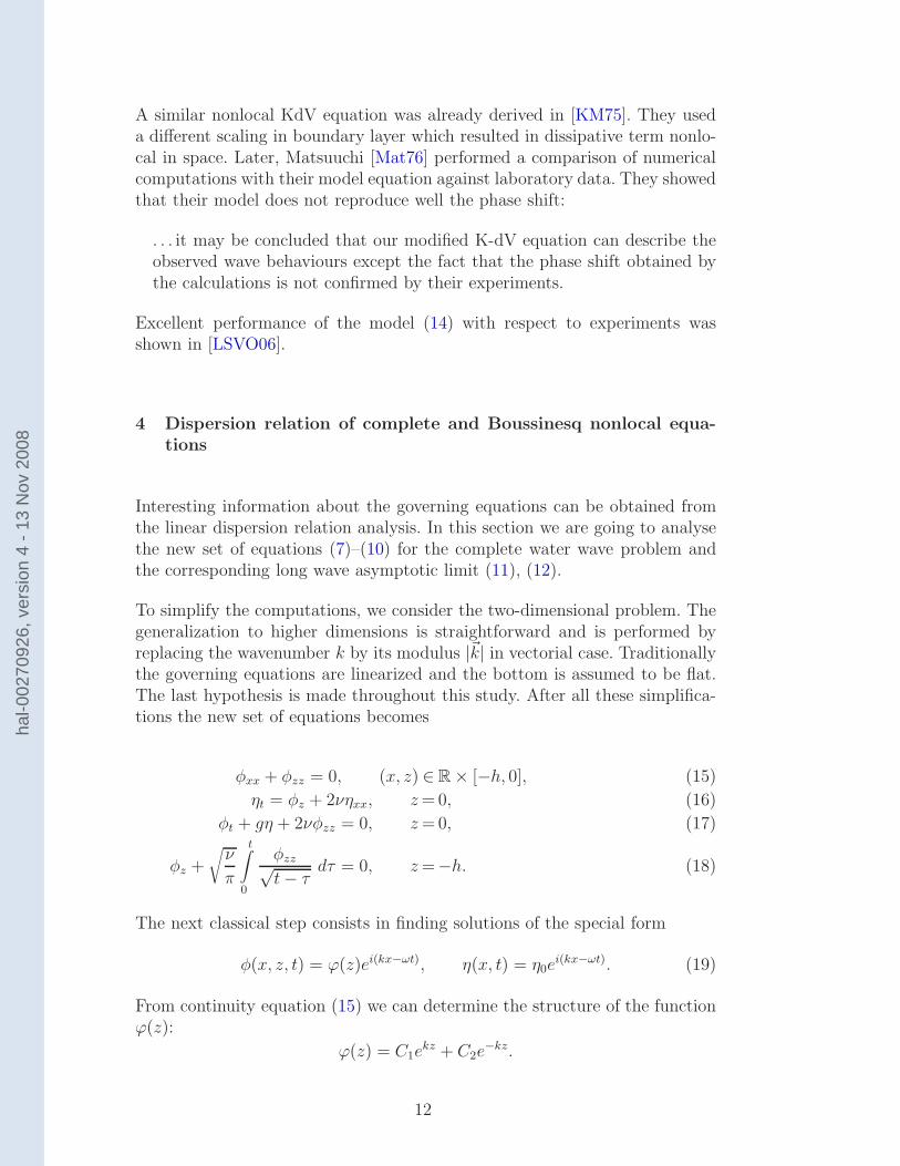
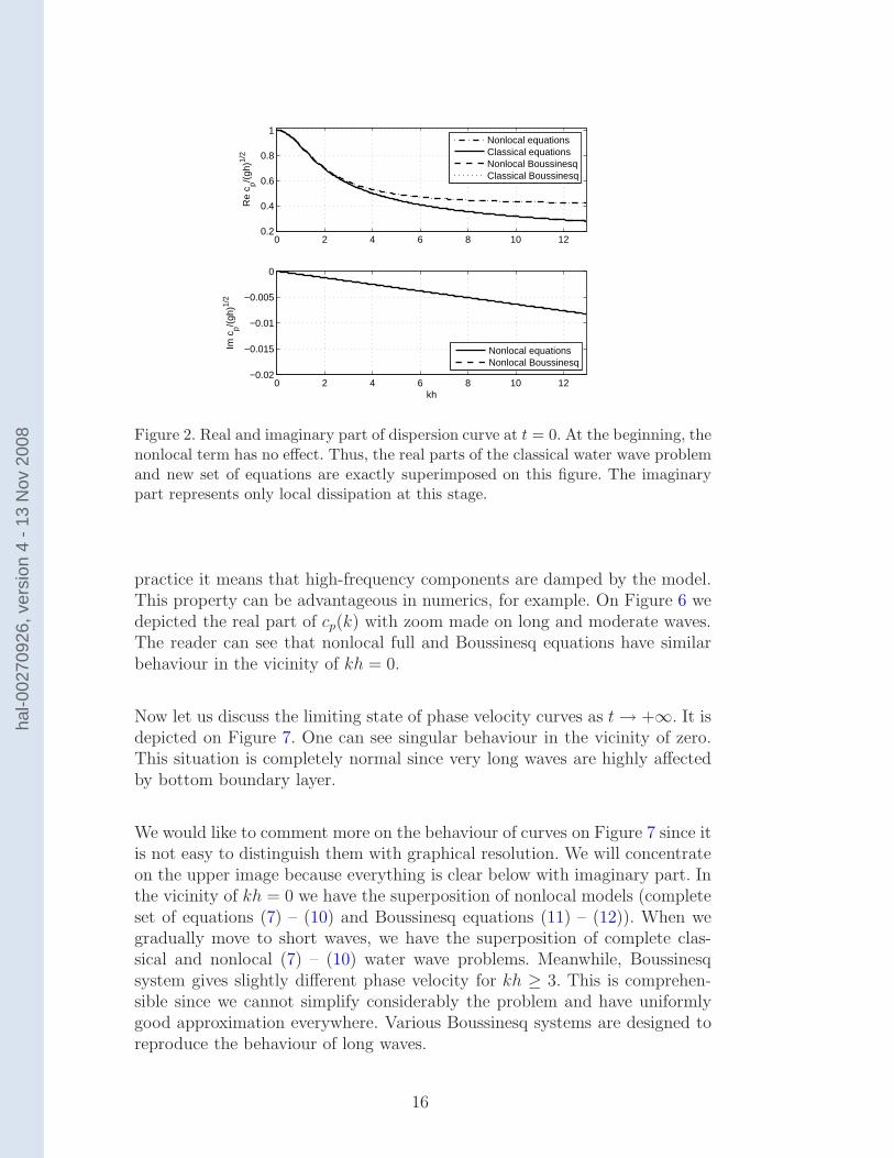
Just at the beginning (when t = 0), there is no effect of the nonlocal term.This is why on Figure 2 new and classical 4 curves are superimposed. With nosurprise, the phase velocity of Boussinesq equations represents well only longwaves limit (let us say up to kh ≈ 2). When time evolves, we can see that themain effect of nonlocal term consists in slowing down long waves (see Figures3–5). Namely, in the vicinity of kh = 0 the real part of the phase velocityis slightly smaller with respect to the classical formulation. From physicalpoint of view this situation is comprehensible since only long waves “feel” thebottom and, by consequence, are affected by bottom boundary layer. On theother hand, the imaginary part of the phase velocity is responsible for the waveamplitude attenuation. The minimum of Im cp(k) in the region of long wavesindicates that there is a “preferred” wavelength which is attenuated the most.In the range of short waves the imaginary part is monotonically decreasing. In

3 To be precise, we plot real and imaginary parts of the dimensionless phase velocitywhich is defined as cp(k) := 1√

gh

ω(k)k

.

4 In this section expression “classical” refers to complete water wave problem or itsdispersion relation correspondingly.

15

hal-0

0270

926,

ver

sion

4 -

13 N

ov 2

008

0 2 4 6 8 10 120.2

0.4

0.6

0.8

1

Re

c p/(gh

)1/2

Nonlocal equationsClassical equationsNonlocal BoussinesqClassical Boussinesq

0 2 4 6 8 10 12−0.02

−0.015

−0.01

−0.005

0

kh

Im c

p/(gh

)1/2

Nonlocal equationsNonlocal Boussinesq

Figure 2. Real and imaginary part of dispersion curve at t = 0. At the beginning, thenonlocal term has no effect. Thus, the real parts of the classical water wave problemand new set of equations are exactly superimposed on this figure. The imaginarypart represents only local dissipation at this stage.

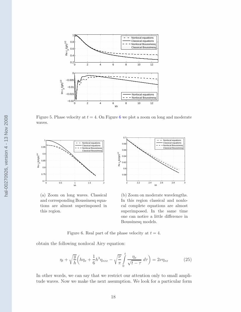
practice it means that high-frequency components are damped by the model.This property can be advantageous in numerics, for example. On Figure 6 wedepicted the real part of cp(k) with zoom made on long and moderate waves.The reader can see that nonlocal full and Boussinesq equations have similarbehaviour in the vicinity of kh = 0.

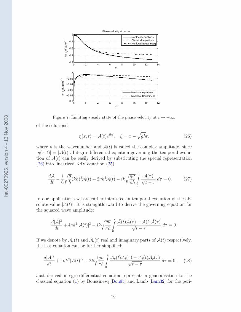
Now let us discuss the limiting state of phase velocity curves as t→ +∞. It isdepicted on Figure 7. One can see singular behaviour in the vicinity of zero.This situation is completely normal since very long waves are highly affectedby bottom boundary layer.

We would like to comment more on the behaviour of curves on Figure 7 since itis not easy to distinguish them with graphical resolution. We will concentrateon the upper image because everything is clear below with imaginary part. Inthe vicinity of kh = 0 we have the superposition of nonlocal models (completeset of equations (7) – (10) and Boussinesq equations (11) – (12)). When wegradually move to short waves, we have the superposition of complete clas-sical and nonlocal (7) – (10) water wave problems. Meanwhile, Boussinesqsystem gives slightly different phase velocity for kh ≥ 3. This is comprehen-sible since we cannot simplify considerably the problem and have uniformlygood approximation everywhere. Various Boussinesq systems are designed toreproduce the behaviour of long waves.

16

hal-0

0270

926,

ver

sion

4 -

13 N

ov 2

008

0 2 4 6 8 10 120.2

0.4

0.6

0.8

1

Re

c p/(gh

)1/2

0 2 4 6 8 10 12−0.02

−0.015

−0.01

−0.005

0

kh

Im c

p/(gh

)1/2

Nonlocal equationsClassical equationsNonlocal BoussinesqClassical Boussinesq

Nonlocal equationsNonlocal Boussinesq

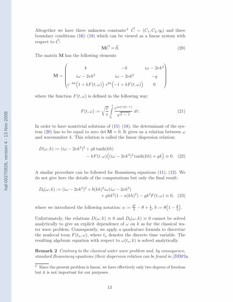
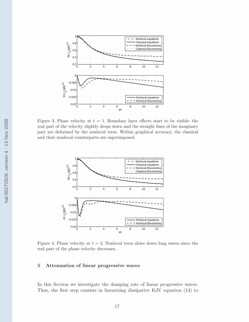
Figure 3. Phase velocity at t = 1. Boundary layer effects start to be visible: thereal part of the velocity slightly drops down and the straight lines of the imaginarypart are deformed by the nonlocal term. Within graphical accuracy, the classicaland their nonlocal counterparts are superimposed.

0 2 4 6 8 10 120.2

0.4

0.6

0.8

1

Re

c p/(gh

)1/2

0 2 4 6 8 10 12−0.02

−0.015

−0.01

−0.005

0

kh

Im c

p/(gh

)1/2

Nonlocal equationsClassical equationsNonlocal BoussinesqClassical Boussinesq

Nonlocal equationsNonlocal Boussinesq

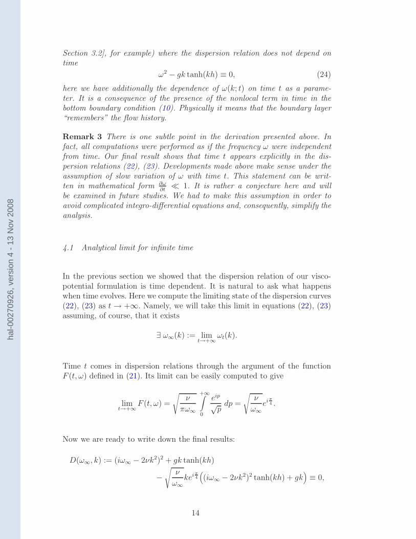
Figure 4. Phase velocity at t = 2. Nonlocal term slows down long waves since thereal part of the phase velocity decreases.

5 Attenuation of linear progressive waves

In this Section we investigate the damping rate of linear progressive waves.Thus, the first step consists in linearizing dissipative KdV equation (14) to

17

hal-0

0270

926,

ver

sion

4 -

13 N

ov 2

008

0 2 4 6 8 10 120.2

0.4

0.6

0.8

1

Re

c p/(gh

)1/2

0 2 4 6 8 10 12−0.02

−0.015

−0.01

−0.005

0

kh

Im c

p/(gh

)1/2

Nonlocal equationsClassical equationsNonlocal BoussinesqClassical Boussinesq

Nonlocal equationsNonlocal Boussinesq

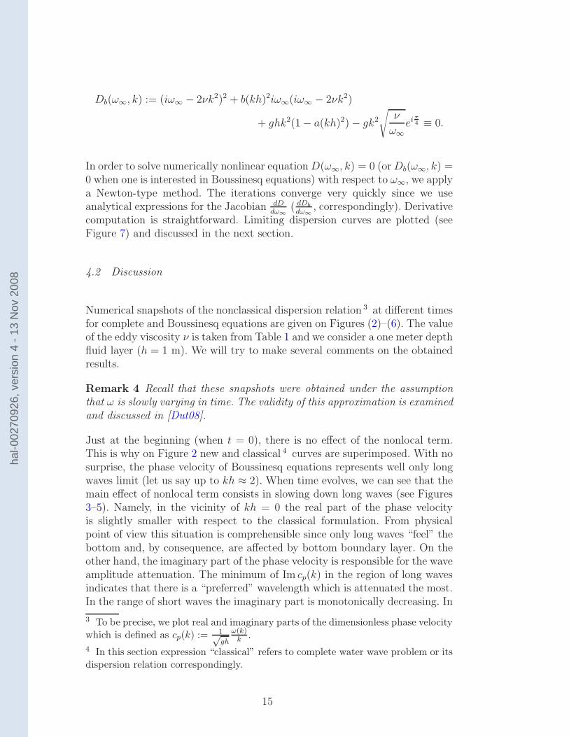
Figure 5. Phase velocity at t = 4. On Figure 6 we plot a zoom on long and moderatewaves.

0 0.5 1 1.5 20.7

0.75

0.8

0.85

0.9

0.95

1

kh

Re

c p(k)/

(gh)

1/2

Nonlocal equationsClassical equationsNonlocal BoussinesqClassical Boussinesq

(a) Zoom on long waves. Classicaland corresponding Boussinesq equa-tions are almost superimposed inthis region.

2 2.2 2.4 2.6 2.8 3

0.58

0.6

0.62

0.64

0.66

0.68

0.7

kh

Re

c p(k)/

(gh)

1/2

Nonlocal equationsClassical equationsNonlocal BoussinesqClassical Boussinesq

(b) Zoom on moderate wavelengths.In this region classical and nonlo-cal complete equations are almostsuperimposed. In the same timeone can notice a little difference inBoussinesq models.

Figure 6. Real part of the phase velocity at t = 4.

obtain the following nonlocal Airy equation:

ηt +

√g

h

(

hηx +1

6h3ηxxx −

√ν

π

t∫

0

ηx√t− τ

dτ)

= 2νηxx (25)

In other words, we can say that we restrict our attention only to small ampli-tude waves. Now we make the next assumption. We look for a particular form

18

hal-0

0270

926,

ver

sion

4 -

13 N

ov 2

008

0 2 4 6 8 10 12 140.2

0.4

0.6

0.8

1

khR

e c p(k

)/(g

h)1/

2

Phase velocity at t = +∞

Nonlocal equationsClassical equationsNonlocal Boussinesq

0 2 4 6 8 10 12 14−0.1

−0.08

−0.06

−0.04

−0.02

0

kh

Im c

p(k)/

(gh)

1/2

Nonlocal equationsNonlocal Boussinesq

Figure 7. Limiting steady state of the phase velocity at t → +∞.

of the solutions:

η(x, t) = A(t)eikξ, ξ = x−√

ght. (26)

where k is the wavenumber and A(t) is called the complex amplitude, since|η(x, t)| = |A(t)|. Integro-differential equation governing the temporal evolu-tion of A(t) can be easily derived by substituting the special representation(26) into linearized KdV equation (25):

dAdt

− i

6

√g

h(kh)3A(t) + 2νk2A(t) − ik

√gν

πh

t∫

0

A(τ)√t− τ

dτ = 0. (27)

In our applications we are rather interested in temporal evolution of the ab-solute value |A(t)|. It is straightforward to derive the governing equation forthe squared wave amplitude:

d|A|2dt

+ 4νk2|A(t)|2 − ik

√gν

πh

t∫

0

A(t)A(τ) −A(t)A(τ)√t− τ

dτ = 0.

If we denote by Ar(t) and Ai(t) real and imaginary parts of A(t) respectively,the last equation can be further simplified:

d|A|2dt

+ 4νk2|A(t)|2 + 2k

√gν

πh

t∫

0

Ar(t)Ai(τ) −Ai(t)Ar(τ)√t− τ

dτ = 0. (28)

Just derived integro-differential equation represents a generalisation to theclassical equation (1) by Boussinesq [Bou95] and Lamb [Lam32] for the peri-

19

hal-0

0270

926,

ver

sion

4 -

13 N

ov 2

008

odic, linear wave amplitude evolution in a viscous fluid. We recall that novelintegral term is a direct consequence of the bottom boundary layer modelling.

Unfortunately, equation (28) cannot be used directly for numerical computa-tions since we need to know the following combination of real and imaginaryparts Ar(t)Ai(τ) − Ai(t)Ar(τ) for τ ∈ [0, t]. It represents a new and non-classical aspect of the present theory.

Equation (28) allows us to discuss the relative importance of local and nonlo-cal dissipative terms for long waves. In fact, when we consider the deep-waterapproximation, only local dissipative terms are present in the governing equa-tions [DDZ08]. On the other hand, in shallow waters the integral term ispredominant. It means that there is an intermediate depth where both dissi-pative terms have equal magnitude. This depth can be estimated when oneswitches to dimensionless form of the equation (28). Comparing the coeffi-cients in front of dissipative terms gives the following transcendental equationfor the “critical” depth h∗:

h∗ =g

4πωνk2

where ω is the characteristic wave frequency.

In numerical computations it is advantageous to integrate exactly local termsin equation (27). It is done by making the following change of variables:

A(t) = e−2νk2tei6

√g

h(kh)3tA(t).

One can easily show that new function A(t) satisfies the following equation:

dAdt

= ik

√gν

πh

t∫

0

e2νk2(t−τ)e−

i6

√g

h(kh)3(t−τ)

√t− τ

A(τ) dτ

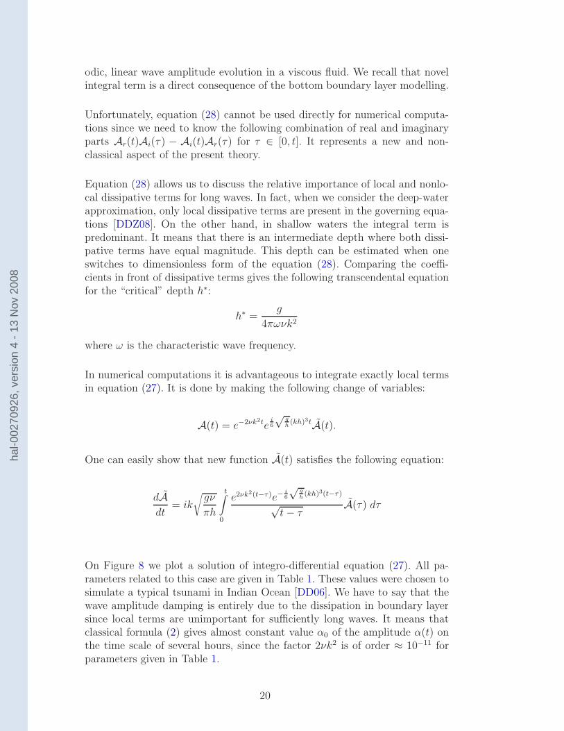
On Figure 8 we plot a solution of integro-differential equation (27). All pa-rameters related to this case are given in Table 1. These values were chosen tosimulate a typical tsunami in Indian Ocean [DD06]. We have to say that thewave amplitude damping is entirely due to the dissipation in boundary layersince local terms are unimportant for sufficiently long waves. It means thatclassical formula (2) gives almost constant value α0 of the amplitude α(t) onthe time scale of several hours, since the factor 2νk2 is of order ≈ 10−11 forparameters given in Table 1.

20

hal-0

0270

926,

ver

sion

4 -

13 N

ov 2

008

parameter definition value

ν eddy viscosity 10−3 m2

s

g gravity acceleration 9.8 ms2

h water depth 3600 m

ℓ wavelength 50 km

k wavenumber = 2πℓ

m−1

Table 1Values of the parameters used in the numerical computations of the linear progres-sive waves amplitude. These values correspond to a typical Indian Ocean tsunami.

0 1 2 3 4 5 60.9

0.92

0.94

0.96

0.98

1

1.02

t, hours

|A(t

)|/|A

(0)|

Amplitude of linear progressive waves

Figure 8. Amplitude of linear progressive waves as a function of time. Values of allparameters are given in Table 1.

6 Solitary wave propagation

In this section we would like to show the effect of nonlocal term on the solitarywave attenuation. For simplicity, we will consider wave propagation in a 1Dchannel. The question of the bottom shear stress effect on the solitary wavepropagation was considered for the first time in [Keu48].

For numerical integration of equations (11), (12) we use the same Fourier-type spectral method that was described in [DD07a, Section 5]. Obviouslythis method has to be slightly adapted because of the presence of nonlocalin time term. We have to say that this term necessitates the storage of ∇ ·~u(n) at previous time steps. Hence, long time computations can be memoryconsuming.

21

hal-0

0270

926,

ver

sion

4 -

13 N

ov 2

008

The values of all dimensionless parameters are given in Table 2. Dimensionlessviscosity ν is related to other physical parameters in the following way:

ν2 =ν

ℓ√gh,

where ν is kinematic viscosity, ℓ is the characteristic wavelength and h is thetypical depth.

Remark 5 From numerical point of view, the integral termt∫

0

φzz(~x,−h,τ)√t−τ dτ

can pose some problems in the vicinity of the upper limit τ = t. Probably thebest way to deal with this problem is to separate the integral in two parts:

t∫

0

φzz(~x,−h, τ)√t− τ

dτ =

t−δ∫

0

φzz(~x,−h, τ)√t− τ

dτ +

t∫

t−δ

φzz(~x,−h, τ)√t− τ

dτ, δ > 0.

The first integral can be computed in a usual way without any special care.Then one applies to the second integral a special class of Gauss quadratureformulas with weighting function (t− τ)−

1

2 .

But there is another well-known trick that we describe here. This techniquecan be implemented in simpler way. We rewrite our integral in the followingway

t∫

0

φzz(~x,−h, τ)√t− τ

dτ =

t∫

0

φzz(~x,−h, t)√t− τ

dτ +

t∫

0

φzz(~x,−h, τ) − φzz(~x,−h, t)√t− τ

dτ.

The first integral in the right hand side can be evaluated analytically while thesecond one does not contain any singularity under the assumption of differen-tiability of τ 7→ φzz(~x,−h, τ) at τ = t:

t∫

0

φzz(~x,−h, τ)√t− τ

dτ = 2√tφzz(~x,−h, t) +

t∫

0

φzz(~x,−h, τ) − φzz(~x,−h, t)√t− τ

dτ.

Remark 6 What is the value of ν to be taken in numerical simulations? Thereis surprisingly little published information of this subject. What is clear is thatthe molecular diffusion is too small to model true viscous damping and oneshould rather consider the eddy viscosity parameter. Some interesting infor-mation on this subject can be found in [TSL07]:

We have spent a considerable amount of time and effort seeking furtherpublished information on viscous effects on ship waves.

This sentence confirms our apprehension. The authors of this work came tothe following conclusion

22

hal-0

0270

926,

ver

sion

4 -

13 N

ov 2

008

parameter definition value

ε nonlinearity 0.02

µ dispersion 0.06

ν eddy viscosity 0.001

c soliton velocity 1.02

θ zθ = −θh 1 −√

5/5

x0 soliton center at t = 0 −1.5

Table 2Values of the dimensionless parameters used in the numerical computations.

. . . we reiterate that a viscosity of about ν = 0.005 m2/s gave reason-able agreement with longitudinal cut results (including apparent dampingof transverse waves).

In another famous paper [BPS81] one can find:

. . . Such a decay rate leads to a value for µ in (M∗) of 0.014. . .

In their work µ is the coefficient in front of the dissipative term in BBMequation:

ηt + ηx +3

2ηηx − µηxx −

1

6ηxxt = 0.

It is important to underline that this equation is written in dimensionlessvariables. Thus, the value reported in that study has to be rescaled with respectto other physical parameters.

Liu and Orfilla [LO04] report the value of eddy viscosity ν = 0.001 m2/s.

If we summarize all the remarks made above, we can conclude that the valueof the order 10−3 – 10−2 m2/s should give reasonable results.

6.1 Approximate solitary wave solution

In order to provide an initial condition for equations (11), (12), we are goingto obtain an approximate solitary wave solution for nondissipative 1D versionof these equations over the flat bottom:

ηt +(

(1 + εη)u)

x+ µ2

(θ2

2− θ +

1

3

)

uxxx= 0,

ut + ηx +ε

2(u2)x − µ2θ

(

1 − θ

2

)

uxxt= 0.

23

hal-0

0270

926,

ver

sion

4 -

13 N

ov 2

008

−3 −2 −1 0 1 2 3

0

0.2

0.4

0.6

0.8

1

1.2

1.4

1.6

1.8

2

t = 0.500

x

η

No dissipationLocalNonlocal

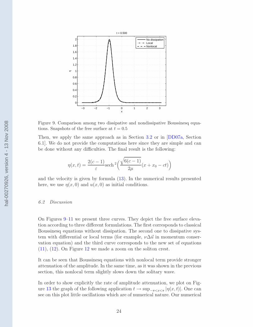
Figure 9. Comparison among two dissipative and nondissipative Boussinesq equa-tions. Snapshots of the free surface at t = 0.5

Then, we apply the same approach as in Section 3.2 or in [DD07a, Section6.1]. We do not provide the computations here since they are simple and canbe done without any difficulties. The final result is the following:

η(x, t) =2(c− 1)

εsech 2

(√

6(c− 1)

2µ(x+ x0 − ct)

)

and the velocity is given by formula (13). In the numerical results presentedhere, we use η(x, 0) and u(x, 0) as initial conditions.

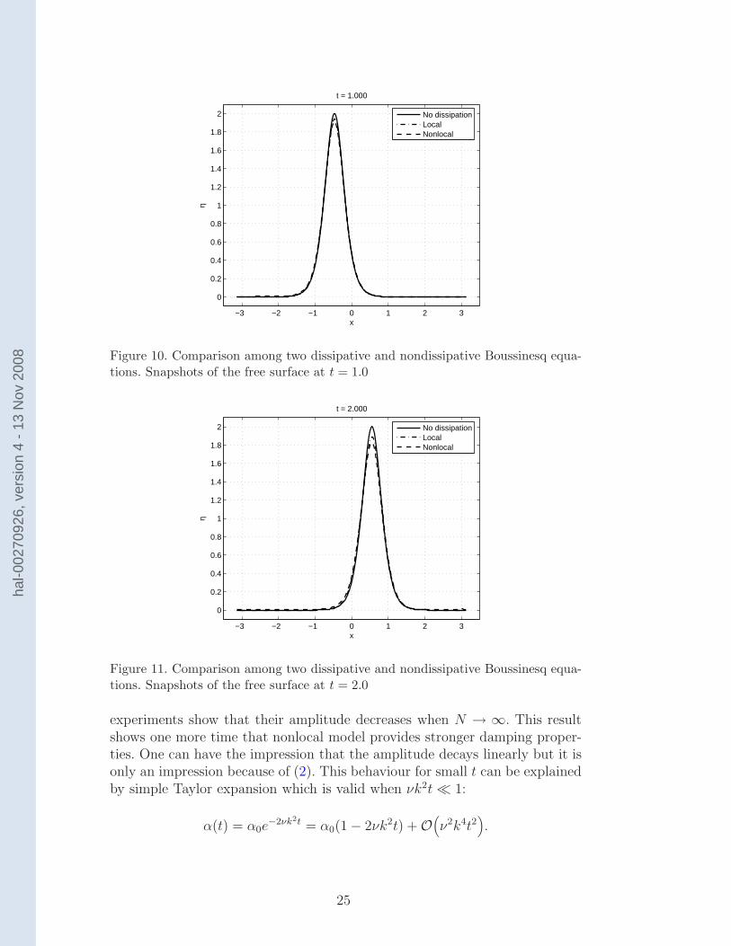
6.2 Discussion

On Figures 9–11 we present three curves. They depict the free surface eleva-tion according to three different formulations. The first corresponds to classicalBoussinesq equations without dissipation. The second one to dissipative sys-tem with differential or local terms (for example, ν∆~u in momentum conser-vation equation) and the third curve corresponds to the new set of equations(11), (12). On Figure 12 we made a zoom on the soliton crest.

It can be seen that Boussinesq equations with nonlocal term provide strongerattenuation of the amplitude. In the same time, as it was shown in the previoussection, this nonlocal term slightly slows down the solitary wave.

In order to show explicitly the rate of amplitude attenuation, we plot on Fig-ure 13 the graph of the following application t→ sup−π<x<π |η(x, t)|. One cansee on this plot little oscillations which are of numerical nature. Our numerical

24

hal-0

0270

926,

ver

sion

4 -

13 N

ov 2

008

−3 −2 −1 0 1 2 3

0

0.2

0.4

0.6

0.8

1

1.2

1.4

1.6

1.8

2

t = 1.000

x

η

No dissipationLocalNonlocal

Figure 10. Comparison among two dissipative and nondissipative Boussinesq equa-tions. Snapshots of the free surface at t = 1.0

−3 −2 −1 0 1 2 3

0

0.2

0.4

0.6

0.8

1

1.2

1.4

1.6

1.8

2

t = 2.000

x

η

No dissipationLocalNonlocal

Figure 11. Comparison among two dissipative and nondissipative Boussinesq equa-tions. Snapshots of the free surface at t = 2.0

experiments show that their amplitude decreases when N → ∞. This resultshows one more time that nonlocal model provides stronger damping proper-ties. One can have the impression that the amplitude decays linearly but it isonly an impression because of (2). This behaviour for small t can be explainedby simple Taylor expansion which is valid when νk2t≪ 1:

α(t) = α0e−2νk2t = α0(1 − 2νk2t) + O

(

ν2k4t2)

.

25

hal-0

0270

926,

ver

sion

4 -

13 N

ov 2

008

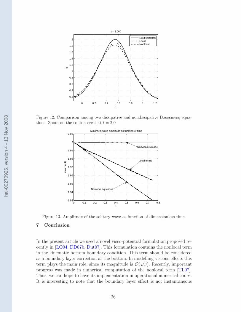
0 0.2 0.4 0.6 0.8 1 1.2

0.2

0.4

0.6

0.8

1

1.2

1.4

1.6

1.8

2

t = 2.000

x

η

No dissipationLocalNonlocal

Figure 12. Comparison among two dissipative and nondissipative Boussinesq equa-tions. Zoom on the soliton crest at t = 2.0

0 0.1 0.2 0.3 0.4 0.5 0.6 0.7 0.81.93

1.94

1.95

1.96

1.97

1.98

1.99

2

2.01

t

max

η(x

,t)

Maximum wave amplitude as function of time

Nonviscous model

Nonlocal equations

Local terms

Figure 13. Amplitude of the solitary wave as function of dimensionless time.

7 Conclusion

In the present article we used a novel visco-potential formulation proposed re-cently in [LO04, DD07b, Dut07]. This formulation contains the nonlocal termin the kinematic bottom boundary condition. This term should be consideredas a boundary layer correction at the bottom. In modelling viscous effects thisterm plays the main role, since its magnitude is O(

√ν). Recently, important

progress was made in numerical computation of the nonlocal term [TL07].Thus, we can hope to have its implementation in operational numerical codes.It is interesting to note that the boundary layer effect is not instantaneous

26

hal-0

0270

926,

ver

sion

4 -

13 N

ov 2

008

but rather cumulative. The flow history is weighted by (t− τ)−1

2 in favour ofthe current time t. As pointed out in [LO04], this nonlocal term is essential tohave an accurate estimation of the bottom shear stress based on the calculatedwave field above the bed. Then, this information can be used for calculatingsediment-bedload transport fluxes and, in turn, morphological changes.

A long wave asymptotic limits (Boussinesq and KdV equations) were derivedfrom this new formulation. The dispersion relation was described. Due to thepresence of special functions, we cannot obtain a simple analytical dependenceof the frequency ω on the wavenumber k as in classical equations. Consequentlythe dispersion curve was obtained numerically by a Newton-type method. Wemade a comparison between the phase velocity of the complete visco-potentialproblem and the corresponding Boussinesq equations. The dispersion relationof new formulation is shown to be time dependent and this property is notclassical. It comes from the memory effect of the boundary layer. We computedanalytically the limiting dispersion curve ω∞(k) as t→ +∞.

The effect of the nonlocal term on the solitary wave attenuation was inves-tigated numerically with a Fourier-type spectral method. We showed that itprovides much stronger damping (see Figure 13). An equation describing theamplitude evolution of linear progressive waves was derived (27). This resultincludes bottom boundary layer correction and generalizes classical formula(1) by Boussinesq [Bou95] and Lamb [Lam32].

The present study opens new exciting possibilities for future research. Namely,we did not consider at all the questions of theoretical justification of visco-potential formulation and corresponding long wave models in the spirit ofworks by J. Bona, J.-C. Saut, D. Lannes, T. Colin [BCL05, BCS02]. Otherdirections for future work consist in implementing new visco-potential frame-work in operational ocean and nearshore models.

Acknowledgment

The author of this paper would like to express his gratitude to professorsFrederic Dias and Jean-Claude Saut for very helpful discussions.

References

[BCL05] J.L. Bona, T. Colin, and D. Lannes. Long wave approximationsfor water waves. Arch. Rational Mech. Anal., 178:373–410, 2005.27

27

hal-0

0270

926,

ver

sion

4 -

13 N

ov 2

008

[BCS02] J.L. Bona, M. Chen, and J.-C. Saut. Boussinesq equations andother systems for small-amplitude long waves in nonlinear disper-sive media. I: Derivation and linear theory. Journal of NonlinearScience, 12:283–318, 2002. 27

[Bou95] J. Boussinesq. Lois de l’extinction de la houle en haute mer. C. R.Acad. Sci. Paris, 121:15–20, 1895. 2, 19, 27

[BPS81] J.L. Bona, W.G. Pritchard, and L.R. Scott. An evaluation of amodel equation for water waves. Phil. Trans. R. Soc. Lond. A,302:457–510, 1981. 3, 23

[BS71] J.G.B. Byatt-Smith. The effect of laminar viscosity on the solutionof the undular bore. J. Fluid Mech., 48:33–40, 1971. 11

[CG07] M. Chen and O. Goubet. Long-time asymptotic behaviour of dis-sipative Boussinesq systems. Discrete and Continuous DynamicalSystems, 17:61–80, 2007. 4

[Che68] W. Chester. Resonant oscillations of water waves. I. theory. Pro-ceedings of the Royal Society of London. Series A, Mathematicaland Physical Sciences, 306(1484):5–22, 1968. 11

[DD06] F. Dias and D. Dutykh. Extreme Man-Made and Natural Hazardsin Dynamics of Structures, chapter Dynamics of tsunami waves,pages 35–60. Springer, 2006. 4, 20

[DD07a] D. Dutykh and F. Dias. Dissipative Boussinesq equations. C. R.Mecanique, 335:559–583, 2007. 3, 4, 10, 11, 13, 21, 24

[DD07b] D. Dutykh and F. Dias. Viscous potential free-surface flows in afluid layer of finite depth. C. R. Acad. Sci. Paris, Ser. I, 345:113–118, 2007. 2, 4, 8, 9, 26

[DDZ08] F. Dias, A.I. Dyachenko, and V.E. Zakharov. Theory of weaklydamped free-surface flows: a new formulation based on potentialflow solutions. Physics Letters A, 372:1297–1302, 2008. 2, 4, 20

[DKZ03] A.I. Dyachenko, A.O. Korotkevich, and V.E. Zakharov. Weak tur-bulence of gravity waves. JETP Lett., 77:546–550, 2003. 4

[DKZ04] A.I. Dyachenko, A.O. Korotkevich, and V.E. Zakharov. Weak tur-bulent Kolmogorov spectrum for surface gravity waves. Phys. Rev.Lett., 92:134501, 2004. 4

[Dut07] D. Dutykh. Mathematical modelling of tsunami waves. PhD thesis,Ecole Normale Superieure de Cachan, 2007. 4, 8, 26

[Dut08] D. Dutykh. Group and phase velocities in the free-surface visco-potential flow: new kind of boundary layer induced instability. Sub-mitted to Physics Letters A, 2008. 15

[GPT03] R. Grimshaw, E. Pelinovsky, and T. Talipova. Damping of large-amplitude solitary waves. Wave Motion, 37:351–364, 2003. 11

[JW04] D.D. Joseph and J. Wang. The dissipation approximation andviscous potential flow. J. Fluid Mech., 505:365–377, 2004. 3

[Keu48] G.H. Keulegan. Gradual damping of solitary waves. J. Res. Nat.Bureau Standards, 40(6):487–498, 1948. 21

[Kha87] G.A. Khabakhpashev. Effect of bottom friction on the dynamics of

28

hal-0

0270

926,

ver

sion

4 -

13 N

ov 2

008

gravity perturbations. Fluid Dynamics, 22(3):430–437, 1987. 10[Kha97] G. A. Khabakhpashev. Nonlinear evolution equation for sufficiently

long two-dimensional waves on the free surface of a viscous liquid.Computational Technologies, 2:94–101, 1997. 4

[KM75] T. Kakutani and K. Matsuuchi. Effect of viscosity on long gravitywaves. J. Phys. Soc. Japan, 39:237–246, 1975. 4, 12

[Lam32] H. Lamb. Hydrodynamics. Cambridge University Press, 1932. 2,10, 19, 27

[LH92] M.S. Longuet-Higgins. Theory of weakly damped stokes waves: anew formulation and its physical interpretation. J. Fluid Mech.,235:319–324, 1992. 1

[Lig78] J. Lighthill. Waves in Fluids. Cambridge University Press, 1978.4

[Liu06] P.L.-F. Liu. Turbulent boundary layer effects on transientwave propagation in shallow water. Proc. Roy. Soc. London,462(2075):3481–3491, 2006. 9

[LO04] P.L.-F. Liu and A. Orfila. Viscous effects on transient long-wavepropagation. J. Fluid Mech., 520:83–92, 2004. 4, 10, 23, 26, 27

[LPC07] P.L.-F. Liu, Y.S. Park, and E.A. Cowen. Boundary layer flow andbed shear stress under a solitary wave. J. Fluid Mech., 574:449–463, 2007. 9

[LSVO06] P.L.-F. Liu, G. Simarro, J. Vandever, and A. Orfila. Experimentaland numerical investigation of viscous effects on solitary wave prop-agation in a wave tank. Coastal Engineering, 53:181–190, 2006. 3,4, 5, 12

[Mat76] K. Matsuuchi. Numerical investigations on long gravity waves un-der the influence of viscosity. J. Phys. Soc. Japan, 41(2):681–686,August 1976. 12

[Mei94] C.C. Mei. The applied dynamics of ocean surface waves. WorldScientific, 1994. 4, 5

[Mil76] J.W. Miles. Korteweg-de Vries equation modified by viscosity.Phys. Fluids, 19(7), 1976. 11

[ML73] C. C. Mei and P.L.-F. Liu. The damping of surface gravity wavesin a bounded liquid. J. Fluid Mech., 59(2):239–256, 1973. 7

[Sug89] N. Sugimoto. Nonlinear wave motion, chapter ’Generalized’ Burg-ers equations and fractional calculus, pages 162–179. LongmanScientific & Technical, 1989. 4

[Sug90] N. Sugimoto. Evolution of nonlinear acoustic waves in a gas-filledpipe. In M.F. Hamilton and D.T. Blackstock, editors, Frontiersof Nonlinear Acoustics, 12th Intl Symp. on Nonlinear Acoustics,1990. 4

[Sug91] N. Sugimoto. Burgers equation with a fractional derivative; hered-itary effects on nonlinear acoustic waves. J. Fluid Mech., 225:631–653, 1991. 4

[TL07] T. Torsvik and P.L.-F. Liu. An efficient method for the numeri-

29

hal-0

0270

926,

ver

sion

4 -

13 N

ov 2

008

cal calculation of viscous effects on transient long-waves. CoastalEngineering, 54:263–269, 2007. 26

[TSL07] E.O. Tuck, D.C. Scullen, and L. Lazauskas. Sea wave patternevaluation. Technical report, The University of Adelaide, 2007.22

[Wu81] T.Y. Wu. Long waves in ocean and coastal waters. Journal ofEngineering Mechanics, 107:501–522, 1981. 2

[Zak68] V.E. Zakharov. Stability of periodic waves of finite amplitude onthe surface of a deep fluid. J. Appl. Mech. Tech. Phys., 9:1990–1994, 1968. 10

[ZG71] N.J. Zabusky and C.C.J. Galvin. Shallow water waves, theKorteweg-de Vries equation and solitons. J. Fluid Mech., 47:811–824, 1971. 2

[ZKPD05] V.E. Zakharov, A.O. Korotkevich, A.N. Pushkarev, and A.I. Dy-achenko. Mesoscopic wave turbulence. JETP Lett., 82:487–491,2005. 4

30

hal-0

0270

926,

ver

sion

4 -

13 N

ov 2

008