VICUS - A Noise Addition Technique for Categorical Data

VICUS - A Noise Addition Technique for Categorical Data

Helen Giggins1 Ljiljana Brankovic2

1 School of Architecture and Built EnvironmentThe University of Newcastle,

University Drive, Callaghan, NSW 2308, AustraliaEmail: [email protected]

2 School of Electrical Engineering and Computer ScienceThe University of Newcastle,

University Drive, Callaghan, NSW 2308, AustraliaEmail: [email protected]

Abstract

Privacy preserving data mining and statistical disclo-sure control have received a great deal of attentionduring the last few decades. Existing techniques aregenerally classified as restriction and data modifica-tion. Within data modification techniques noise addi-tion has been one of the most widely studied but hastraditionally been applied to numerical values, wherethe measure of similarity is straightforward. In thispaper we introduce VICUS, a novel privacy preserv-ing technique that adds noise to categorical data. Ex-perimental evaluation indicates that VICUS performsbetter than random noise addition both in terms ofsecurity and data quality.

1 Introduction

Potential breaches of privacy during statistical anal-ysis or data mining have implications for many facetsof modern society (Brankovic & Estivill-Castro 1999,Giggins & Brankovic 2002, 2003). Privacy preservingdata mining and statistical disclosure control focuson finding a balance between the conflicting goals ofprivacy preservation and data utility (Brankovic &Giggins 2007, Brankovic et al. 2007). Existing tech-niques are generally classified as restriction and datamodification techniques (Brankovic & Giggins 2007).When restriction is applied, a user does not have ac-cess to microdata itself, but rather to a restricted col-lection of statistics (queries). In this context datautility is often referred to as usability, or the percent-age of queries that can be answered without disclo-sure of any sensitive individual value (Brankovic et al.1996a,b). Unfortunately, for general queries the us-ability tends to be very low (Brankovic & Miller 1995,Griggs 1997), especially when higher levels of privacyare required (Griggs 1999). However, if only rangequeries are of interest, which is the case in OLAP,the usability can be very high, providing that all cellsof OLAP cubes contain positive counts (Brankovic

This work was supperted by ARC Discovery ProjectDP0452182.

Copyright c⃝2012, Australian Computer Society, Inc. This pa-per appeared at the 10th Australasian Data Mining Conference(AusDM 2012), Sydney, Australia, December 2012. Confer-ences in Research and Practice in Information Technology (CR-PIT), Vol. 134, Yanchang Zhao, Jiuyong Li, Paul Kennedy, andPeter Christen, Ed. Reproduction for academic, not-for-profitpurposes permitted provided this text is included.

et al. 2000, 2002, Brankovic & Siran 2002, Horak et al.1999, Brankovic et al. 1997).

Unlike restriction, data modification techniques al-low for the microdata to be made available to usersor, alternatively, can provide answers to any query, al-though the answers are not necessarily exact. There-fore, in this context, utility is often equated to dataquality (Islam & Brankovic 2005). In principle, datamodification techniques are applicable to both nu-merical and categorical attributes (Estivill-Castro &Brankovic 1999, Islam & Brankovic 2011); however,techniques such as noise addition are mostly appliedto numerical attributes (Willenborg & de Waal 2001,Muralidhar & Sarathy 2003).

In the context of privacy, there have been twodifferent focal points that attracted the most atten-tion, prevention of membership disclosure (Sweeney2002, Dwork 2006) and prevention of sensitive at-tribute disclosure (Machanavajjhala et al. 2007, Liet al. 2007, Brickell & Shmatikov 2008). Member-ship disclosure refers to revealing the existence of aparticular individual in the database, while sensitiveattribute disclosure occurs when an intruder is ableto learn something about a particular individual’ssensitive information (Brickell & Shmatikov 2008).The k-anonymity privacy requirement introduced bySamarati and Sweeney (Samarati & Sweeney 1998,Sweeney 2002) incorporates generalization to achieveits goal of ensuring that at least k records in the mi-crodata file share values on the set of key attributes(quasi-identifiers). While this approach is success-ful in preventing membership disclosure, it does notprevent sensitive attribute disclosure if (1) there isnot enough diversity in the sensitive attribute, or (2)the malicious user has significant background knowl-edge (Machanavajjhala et al. 2007). The l-diversityprivacy requirement seeks to achieve sensitive at-tribute privacy by applying an additional requirementthat there must exist at least l “well-represented” val-ues of the sensitive attribute in each group of recordssharing quasi-identifier values (Machanavajjhala et al.2007). In the case of very strong backgraound knowl-edge of the intruder, l-diversity may not be suffi-cient to prevent sensitive attribute disclosure (Li et al.2007). A stronger requirements has been proposed,namely t-closeness, which compares the distances be-tween the distributions of sensitive attribute over thewhole microdata file to those for each grouping ofrecords based on the quasi-identifiers (Li et al. 2007).

Differential privacy (Dwork 2006) attempts to cap-ture the notion that one’s privacy should not be atany greater risk of being violated by having one’s in-formation placed in the microdata file. This principleis applied to answering queries via an output pertur-

Proceedings of the Tenth Australasian Data Mining Conference (AusDM 2012), Sydney, Australia

139

Client Branch Financial Product Advisor

Dr T. Green (1) Hong Kong (7) Income Protection Insurance (10) Mr D. Smith (14)Mr D. Blue (2) Hong Kong (7) Home Mortgage (11) Mr D. Smith (14)

Mr M. Brown (3) Newcastle (8) Managed Investment (12) Mr R. Jones (15)Mrs H. Pink (4) Newcastle (8) Share Portfolio (13) Ms W. Wong (16)Mr K. White (5) Sydney (9) Share Portfolio (13) Ms W. Wong (16)Mr J. Black (6) Sydney (9) Managed Investment (12) Ms W. Wong (16)Mr J. Black (6) Sydney (9) Home Mortgage (11) Mr M. James (17)

Table 1: Bank Client Microdata File - Sample

bation technique in (Dwork et al. 2006).In this paper we focus on sensitive attribute disclo-

sure, namely we aim to minimise the information anintruder is able to reveal about a sensitive attributevalue belonging to an individual in the microdata file.By focusing on microdata files containing categoricaldata we are also limited in the way in which we canapply existing privacy requirements and SCD tech-niques. For instance, having no natural ordering ofcategories in an attribute makes the application ofgeneralization techniques difficult when there is noobvious hierarchy to the values. Within data modifi-cation techniques noise addition had been one of themost widely studied, but have traditionally been ap-plied to numerical values (see for example (Muralid-har & Sarathy 2003), and when the data set containscategorical values the application of these techniquestends to be much less straightforward (Willenborg &de Waal 2001). In this paper we introduce “VICUS”,a novel noise addition technique for categorical at-tributes. An important step in VICUS is the cluster-ing of categorical values while, in turn, an importantcomponent of any clustering technique is the notion ofsimilarity between the attribute values. VICUS seeksto maximise the similarity between values in the samecluster, while minimising the similarity between val-ues from different clusters.

In the next section we outline the similarity mea-sure that will be employed in VICUS in Section 3. Wefirst outline the motivation for the similarity measure,before formally defining it. We then present experi-mental results on several different data sets, whichhighlight the effectiveness of our measure. In Section3 we propose VICUS, a noise addition technique forcategorical values, which incorporates our similaritymeasure and assigns transition probabilities based onthe discovered clusters of attribute values. We alsoprovide an analysis of experimental results to see howwell VICUS performs in the conflicting areas of secu-rity and data quality. We provide some concludingremarks in Section 4.

2 Similarity Measure

2.1 Motivating Example

The following example is designed to illustrate the re-lationships that exist in the microdata file, and howVICUS attempts to capture these relationships. Ta-ble 1 shows a sample Bank Client microdata file forcustomers buying financial products from a fictionalbank and similar examples can be constructed frommedical, marketing or criminal research area.

On examining Table 1 we can clearly see a connec-tion between Dr Green and Mr Blue, as they are bothcustomers of the Hong Kong branch and both see thesame financial advisor. However, it may not be soobvious that there is a connection between Mr Brownand Mr White as they have no attribute values incommon, have purchased different financial products

and are seen by different financial advisors at differ-ent branches. Nevertheless, these two clients haveboth purchased financial products that require thepurchase of shares, so there should be some notion ofsimilarity between them.

To better understand these connections betweenthe customers we can represent the microdata shownin Table 1 as a graph (see Figure 1). This is done byassigning values that appear in the table to vertices.An edge appears between two vertices when the corre-sponding two values appear together in a record. Notethat each record forms a clique in the graph. The redcircled subgraph in Figure 1 represents record 7, thatis, Mr Black who has a mortgage and is advised byMr James at the Sydney branch.

13

5

916

128

15

4

17

11

2

14

1

10

7

6

3

Figure 1: Motivating example microdata representedas a graph.

Note that we will be evaluating similarity onlybetween vertices corresponding to the values of thesame attribute in the data set, that is, vertices 1-6, 7-9, 10-13 and 14-17. In the sample database MrBlack (vertex 6) has direct similarity with every otherclient except for Dr Green. This direct similarity isindicated by one or more common neighbours of thecorresponding vertices (or, equivalently, by a path oflength two between the vertices).

Figure 1 shows that there are no common neigh-bours of vertex 3 (Mr Brown) and vertex 5 (MrWhite). This effectively means that the records per-taining to Mr White and Mr Brown will have no val-ues in common. So any method only looking at com-mon values (neighbours) would not find these twovalues at all similar. However, looking at the dataset it is clear that there is some transitive similar-ity between Mr Brown and Mr White, as they bothpurchased products which would typically be consid-ered similar in the financial context. Although theproducts purchased by Mr White and Mr Brown wereprovided by different financial advisors, Mr R. Jonesand Ms W. Wong, these two staff are considered simi-lar because they both sell managed investment funds.Thus, MrWhite and Mr Brown do indeed have similarproducts and are serviced by advisors of similar ex-pertise. Consequently, we may still wish to considerMr White and Mr Brown as similar. Our method

CRPIT Volume 134 - Data Mining and Analytics 2012

140

captures this kind of similarity by looking not just atcommon neighbours of two vertices, but also at com-mon neighbours of their neighbours. We now outlinehow this type of similarity can be measured.

2.2 Evaluating Similarity

The first step in calculating similarity between at-tribute values is to create a corresponding graph,where there is an edge between vertices when two cor-responding values appear together in a record. Notethat we have considered both the simple graph andmultigraph created from the data set. In the simplegraph we create an edge between two attribute val-ues if they co-occur in any record. In the multigraphform we count the number of co-occurrences of thetwo values and consider this as the number of edgesbetween the two corresponding vertices.

The first type of similarity we consider is based onthe values co-occurring in records. For example, inthe Bank Client graph (Figure 1), we would considerthat Dr Green and Mr Blue are similar since theysee the same financial advisor at the same branch.This type of similarity, which we term S

′similarity,

is measured by the number of common neighbours ofthese two vertices in the graph. Looking at Figure 1we see that vertex 1 (Dr Green) and vertex 2 (MrBlue) are both adjacent to vertex 7 (Hong Kong) andvertex 14 (Mr D. Smith). We consider this as a highsimilarity since these two values share a majority ofneighbours in the graph.

The second type of similarity examines ‘neigh-bours of neighbours’ and we denote it as S

′′similarity,

and measure it by first considering the S′similarity

of ‘neighbours’. An example of this type of similar-ity as discussed in Section 2.1 is between Mr Brownand Mr White, who although do not share any at-tribute values, do have ‘similar’ values. For instance,the Newcastle and Sydney branches would be consid-ered similar via an S

′calculation. Similarly, theMan-

aged Investment is similar to Share Portfolio, and MrR. Jones is similar to Ms W. Wong. This means thatall of the values that Mr Brown and Mr White ap-pear with in the data set are considered similar viaS

′similarity, and hence these two values would have

a high S′′similarity.

The Total Similarity S for two attribute values istaken to be composed of both the S

′and S

′′similarity

for the values. We now provide a formal definition ofour similarity measure S.

We calculate the total similarity Sij as a weighted

sum of the S′

ij and S′′

ij :

Sij = c1 × S′

ij + c2 × S′′

ij (1)

where c1 + c2 = 1. Typical values might be c1 = 0.65and c2 = 0.35. In the next section we experimentwith different values for c1 and c2.

2.2.1 Similarity Measure - Sij

We define a simple graphG = (V,E) on n vertices andm edges, where v ∈ V represents an attribute value inthe data set. An edge {i, j} ∈ E exists between twovertices i, j ∈ V when the values i and j both appeartogether in one or more records in the data set. Theadjacency matrix, A, for graph G will contain a 1in position aij if an edge {ij} appears between thevertices i and j, and 0 otherwise.

Input: Graph G, Threshold TOutput: S

′′values for G

initialise S′′matrix to 0;

for each attribute x ∈ G doget the list of attribute values valx;/* Loop over all pairs of values for

the attribute x */for each value i ∈ valx do

for each value j ∈ valx doinitialise mergedGraph to G;/* Loop over all attributes in

G, excluding x */for each attribute y ∈ G \ x do

get the list of attribute valuesvaly;/* Loop over all pairs of

values in y */for each value c ∈ valy do

for each value d ∈ valy doif (there are egdes ({c, i}and {d, j}) ∨ ({c, j} and{d, i}) in G) ∧ (c and dnot already in the samevertex in mergedGraph)then

if S′

cd > Threshold Tthen

merge vertex c andd in mergedGraph;/* Note: if one

vertex hasalready beenmerged withanother,merge alltogether */

endend

endend

end

S′′

ij = S′

ij calculated onmergedGraph

endend

end

return S′′matrix;

Algorithm 1: Calculating S′′values for graph

G

We define a multigraph H = (V,E) on n verticesand m edges, where v ∈ V represents an attributevalue in the data set. An edge {i, j} ∈ E existsbetween two vertices i, j ∈ V for each record thatcontains both values i and j. We do not allow self-loops in this graph. In the adjacency matrix A formultigraph H, aij is the number of edges appearingbetween the vertices i and j in H.

The S′

ij similarity between two attribute values isgiven by

S′

ij =

n∑k=1

√aik × akj√

d(i)× d(j)(2)

where the sum is over all vertices in the graph G (orH), alm is the adjacency matrix entry for vertices land m (1 ≤ l,m ≤ n) and d(l) is the degree of vertex

l. Note that S′

ij has a maximum value of 1 when the


141

two vertices have all their (d(i) = d(j)) neighboursin common, and a minimum value when two verticeshave no neighbours in common (S

′

ij = 0). S′values

are only calculated within an attribute and not acrossattributes.

The S′′

ij similarity captures a notion of transitivesimilarity for attribute values that are not necessar-ily directly connected to a common neighbour but areconnected to similar values, that is, values which havea S

′

ij value greater than the user defined threshold T .

A basic version of an algorithm for calculating S′′

ij

is shown in Algorithm 1. Note that the actual al-gorithm used in experimental analysis is significantlymore efficient than Algorithm 1.

2.3 Experiments - Similarity

In this section we present the results of experimentsconducted on several data sets to observe the effec-tiveness of our similarity measure. Note that onlya small subset of the full experimental analysis con-ducted is presented in this paper due to space restric-tions.

2.3.1 Data Sets

Several data sets have been selected to best demon-strate various qualities and characteristics of our sim-ilarity measure Sij .

Motivating Example. This is the same data setpresented in Section 2.1, and is used to illustrate ad-vantages of our technique over other similarity mea-sures.

Mushroom. This data set was selected as it containsonly categorical values, and although it is a classifi-cation data set, it has also been studied in the con-text of clustering (Guha et al. 2000). It is obtainedfrom the UCI Machine Learning Repository (Asun-cion & Newman 2007). The original data set con-tains 8124 instances on 23 attributes (including theclass attribute), where we removed any records withmissing values.

ACS PUMS. The American Community Survey(ACS) is conducted annually by the United StatesCensus Bureau and was designed to provide a snap-shot of the community. We took a random sample of20,000 records from the 2006 Housing Records PublicUse Microdata Sample (PUMS) 1 for the whole of theUS. The sub-sample was chosen on only 14 attributesof the available 239, and any records with missingvalues on these attributes was not considered.

2.3.2 Parameter Selection

There is a certain amount of flexibility in the calcu-lation of the similarity measure S. First, there is achoice for the value of the S

′′

ij threshold T , which isin the range [0,1]. One observation on the selection ofthis threshold is that for smaller/sparser graphs thethreshold generally needs to be set at a lower valuethan it does for larger/denser graphs. The secondparameter that needs to be selected is the weightingvalues c1 and c2 in Equation 1 where c1+ c2 = 1, anda typical value choice for these parameters would bec1 = 0.6 and c2 = 0.4. This gives a slightly higherweighting to S

′

ij than to S′′

ij . Finally, we have thechoice of making this graph generated from the data

1http://factfinder.census.gov/home/en/acs pums 2006.html

2 4 6 8 10 12 14 16

2

4

6

8

10

12

14

16

0

0.1

0.2

0.3

0.4

0.5

0.6

0.7

0.8

0.9

1

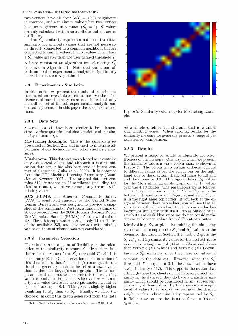
Figure 2: Similarity color map for Motivating Exam-ple.

set a simple graph or a multigraph, that is, a graphwith multiple edges. When showing results for thesimilarity measure we generally present a range of pa-rameters for comparison.

2.3.3 Results

We present a range of results to illustrate the effec-tiveness of our measure. One way in which we presentthe similarity values is via a colour map, as shown inFigure 2. The colour map assigns different coloursto different values as per the colour bar on the righthand side of the diagram. Dark red maps to 1.0 andand dark blue to 0.0. This figure shows Sij valuesfor the Motivating Example graph on all 17 valuesover the 4 attributes. The parameters are as follows;T = 0.4, c1 = 0.6 and c2 = 0.4. Value S1,1 is in thebottom left hand corner of Figure 2, and value S17,17is in the right hand top corner. If you look at the di-agonal between these two values, you will see that allvalues along the diagonal are 1.0, since each value hasmaximum similarity with itself. Areas outside of anattribute are dark blue since we do not consider thesimilarity between values from different attributes.

Motivating Example. Examining the similarityvalues we can compare the S

′

ij and S′′

ij values to thescenarios discussed in Section 2.1. Table 2 gives theS

′

ij , S′′

ij and Sij similarity values for the first attributein our motivating example, that is, Client and showsthat Vertex 5 (Mr White) and Vertex 3 (Mr Brown)

have no S′

ij similarity since they have no values in

common in the data set. However, when the S′′

ij

threshold T is equal to 0.4, these two values havea S

′′

ij similarity of 1.0. This supports the notion thatalthough these two clients do not have any direct sim-ilarity in the data set, they do have a transitive sim-ilarity which should be considered in any subsequentclustering of these values. By the appropriate assign-ment of values to c1 and c2 we can give the desiredweight to this indirect similarity represented by S

′′

ij .In Table 2 we can see the situation for c1 = 0.6 andc2 = 0.4.


142

S′ij 1 2 3 4 5 6

1 1.000 0.667 0.000 0.000 0.000 0.0002 0.667 1.000 0.000 0.000 0.000 0.2583 0.000 0.000 1.000 0.333 0.000 0.2584 0.000 0.000 0.333 1.000 0.667 0.2585 0.000 0.000 0.000 0.667 1.000 0.5166 0.000 0.258 0.258 0.258 0.515 1.000

S′′ij 1 2 3 4 5 6

1 1.000 1.000 0.000 0.000 0.000 0.2582 1.000 1.000 0.000 0.000 0.000 0.2583 0.000 0.000 1.000 1.000 1.000 0.7754 0.000 0.000 1.000 1.000 1.000 0.8825 0.000 0.000 1.000 1.000 1.000 0.8826 0.258 0.258 0.775 0.882 0.882 1.000

Sij 1 2 3 4 5 6

1 1.000 0.800 0.000 0.000 0.000 0.1032 0.800 1.000 0.000 0.000 0.000 0.2583 0.000 0.000 1.000 0.600 0.400 0.4654 0.000 0.000 0.600 1.000 0.800 0.5085 0.000 0.000 0.400 0.800 1.000 0.6636 0.103 0.258 0.465 0.508 0.663 1.000

Table 2: S′

ij , S′′

ij and Sij values for Client attributein Motivating Example.

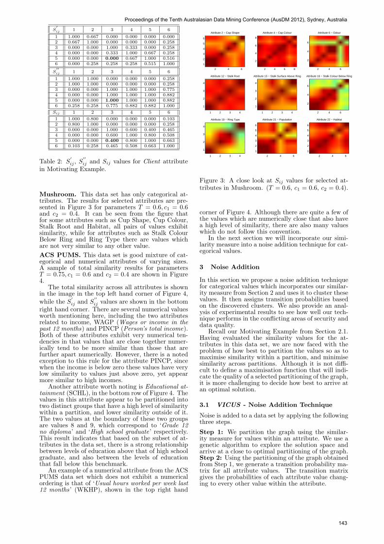
Mushroom. This data set has only categorical at-tributes. The results for selected attributes are pre-sented in Figure 3 for parameters T = 0.6, c1 = 0.6and c2 = 0.4. It can be seen from the figure thatfor some attributes such as Cup Shape, Cup Colour,Stalk Root and Habitat, all pairs of values exhibitsimilarity, while for attributes such as Stalk ColourBelow Ring and Ring Type there are values whichare not very similar to any other value.

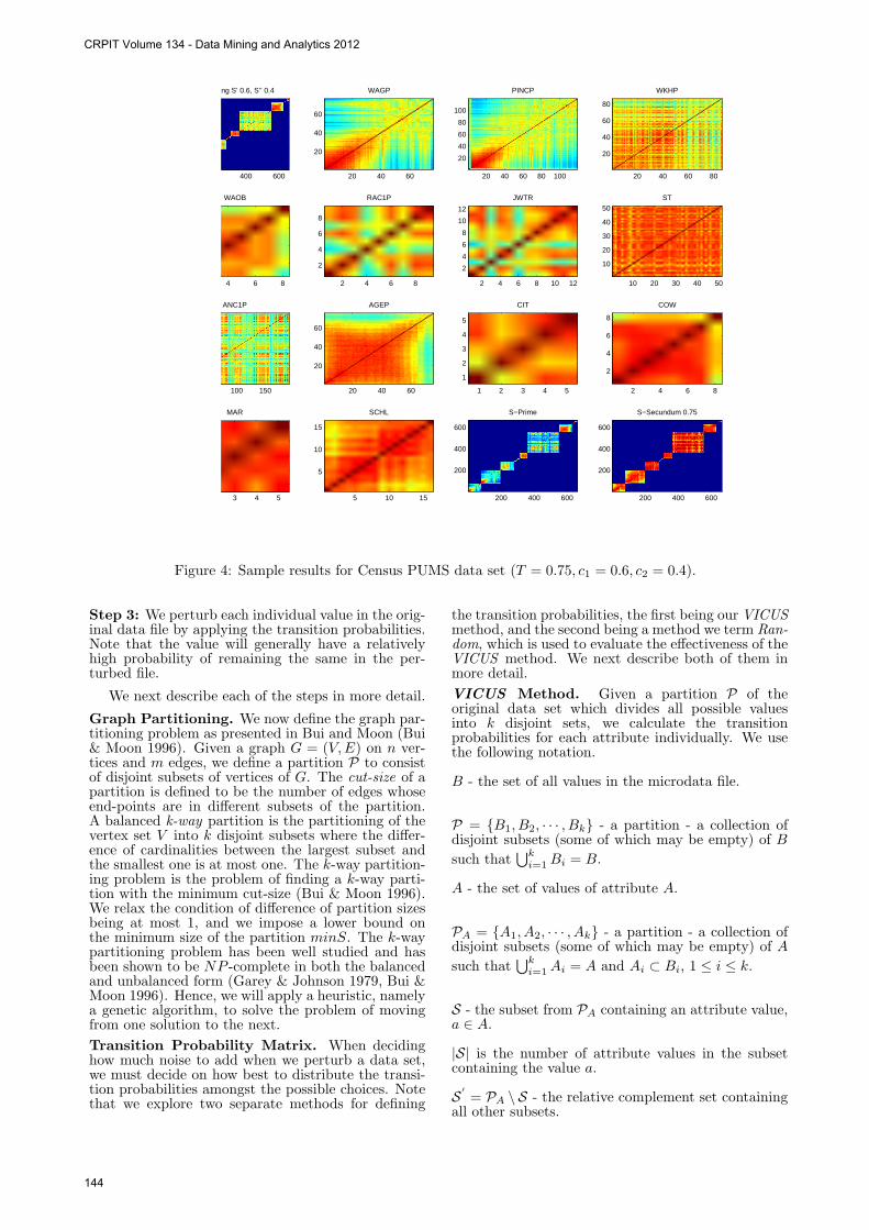
ACS PUMS. This data set is good mixture of cat-egorical and numerical attributes of varying sizes.A sample of total similarity results for parametersT = 0.75, c1 = 0.6 and c2 = 0.4 are shown in Figure4.

The total similarity across all attributes is shownin the image in the top left hand corner of Figure 4,while the S

′

ij and S′′

ij values are shown in the bottomright hand corner. There are several numerical valuesworth mentioning here, including the two attributesrelated to income, WAGP (Wages or income in thepast 12 months) and PINCP (Person’s total income).Both of these attributes exhibit very numerical ten-dencies in that values that are close together numer-ically tend to be more similar than those that arefurther apart numerically. However, there is a notedexception to this rule for the attribute PINCP, sincewhen the income is below zero these values have verylow similarity to values just above zero, yet appearmore similar to high incomes.

Another attribute worth noting is Educational at-tainment (SCHL), in the bottom row of Figure 4. Thevalues in this attribute appear to be partitioned intotwo distinct groups that have a high level of similaritywithin a partition, and lower similarity outside of it.The two values at the boundary of these two groupsare values 8 and 9, which correspond to ‘Grade 12no diploma’ and ‘High school graduate’ respectively.This result indicates that based on the subset of at-tributes in the data set, there is a strong relationshipbetween levels of education above that of high schoolgraduate, and also between the levels of educationthat fall below this benchmark.

An example of a numerical attribute from the ACSPUMS data set which does not exhibit a numericalordering is that of ‘Usual hours worked per week last12 months’ (WKHP), shown in the top right hand

Attribute 2 − Cap Shape

2 4 6

1

2

3

4

5

6

Attribute 4 − Cap Colour

2 4 6 8

2

4

6

8

Attribute 6 − Odour

2 4 6

2

4

6

Attribute 12 − Stalk Root

1 2 3 4

1

2

3

4

Attribute 13 − Stalk Surface Above Ring

1 2 3 4

1

2

3

4

Attribute 16 − Stalk Colour Below Ring

2 4 6

2

4

6

Attribute 19 − Ring Type

1 2 3 4

1

2

3

4

Attribute 21 − Population

2 4 6

1

2

3

4

5

6

Attribute 22 − Habitat

2 4 6

1

2

3

4

5

6

Figure 3: A close look at Sij values for selected at-tributes in Mushroom. (T = 0.6, c1 = 0.6, c2 = 0.4).

corner of Figure 4. Although there are quite a few ofthe values which are numerically close that also havea high level of similarity, there are also many valueswhich do not follow this convention.

In the next section we will incorporate our simi-larity measure into a noise addition technique for cat-egorical values.

3 Noise Addition

In this section we propose a noise addition techniquefor categorical values which incorporates our similar-ity measure from Section 2 and uses it to cluster thesevalues. It then assigns transition probabilities basedon the discovered clusters. We also provide an anal-ysis of experimental results to see how well our tech-nique performs in the conflicting areas of security anddata quality.

Recall our Motivating Example from Section 2.1.Having evaluated the similarity values for the at-tributes in this data set, we are now faced with theproblem of how best to partition the values so as tomaximise similarity within a partition, and minimisesimilarity across partitions. Although it is not diffi-cult to define a maximisation function that will indi-cate the quality of a selected partitioning of the graph,it is more challenging to decide how best to arrive atan optimal solution.

3.1 VICUS - Noise Addition Technique

Noise is added to a data set by applying the followingthree steps.

Step 1: We partition the graph using the similar-ity measure for values within an attribute. We use agenetic algorithm to explore the solution space andarrive at a close to optimal partitioning of the graph.Step 2: Using the partitioning of the graph obtainedfrom Step 1, we generate a transition probability ma-trix for all attribute values. The transition matrixgives the probabilities of each attribute value chang-ing to every other value within the attribute.


143

Weighting S’ 0.6, S’’ 0.4

200 400 600

WAGP

20 40 60

20

40

60

PINCP

20 40 60 80 100

20

40

60

80

100

WKHP

20 40 60 80

20

40

60

80

WAOB

4 6 8

RAC1P

2 4 6 8

2

4

6

8

JWTR

2 4 6 8 10 12

2

4

6

8

10

12

ST

10 20 30 40 50

10

20

30

40

50

ANC1P

100 150

AGEP

20 40 60

20

40

60

CIT

1 2 3 4 5

1

2

3

4

5

COW

2 4 6 8

2

4

6

8

MAR

3 4 5

SCHL

5 10 15

5

10

15

S−Prime

200 400 600

200

400

600

S−Secundum 0.75

200 400 600

200

400

600

Figure 4: Sample results for Census PUMS data set (T = 0.75, c1 = 0.6, c2 = 0.4).

Step 3: We perturb each individual value in the orig-inal data file by applying the transition probabilities.Note that the value will generally have a relativelyhigh probability of remaining the same in the per-turbed file.

We next describe each of the steps in more detail.

Graph Partitioning. We now define the graph par-titioning problem as presented in Bui and Moon (Bui& Moon 1996). Given a graph G = (V,E) on n ver-tices and m edges, we define a partition P to consistof disjoint subsets of vertices of G. The cut-size of apartition is defined to be the number of edges whoseend-points are in different subsets of the partition.A balanced k-way partition is the partitioning of thevertex set V into k disjoint subsets where the differ-ence of cardinalities between the largest subset andthe smallest one is at most one. The k-way partition-ing problem is the problem of finding a k-way parti-tion with the minimum cut-size (Bui & Moon 1996).We relax the condition of difference of partition sizesbeing at most 1, and we impose a lower bound onthe minimum size of the partition minS. The k-waypartitioning problem has been well studied and hasbeen shown to be NP -complete in both the balancedand unbalanced form (Garey & Johnson 1979, Bui &Moon 1996). Hence, we will apply a heuristic, namelya genetic algorithm, to solve the problem of movingfrom one solution to the next.

Transition Probability Matrix. When decidinghow much noise to add when we perturb a data set,we must decide on how best to distribute the transi-tion probabilities amongst the possible choices. Notethat we explore two separate methods for defining

the transition probabilities, the first being our VICUSmethod, and the second being a method we term Ran-dom, which is used to evaluate the effectiveness of theVICUS method. We next describe both of them inmore detail.

VICUS Method. Given a partition P of theoriginal data set which divides all possible valuesinto k disjoint sets, we calculate the transitionprobabilities for each attribute individually. We usethe following notation.

B - the set of all values in the microdata file.

P = {B1, B2, · · · , Bk} - a partition - a collection ofdisjoint subsets (some of which may be empty) of B

such that∪k

i=1 Bi = B.

A - the set of values of attribute A.

PA = {A1, A2, · · · , Ak} - a partition - a collection ofdisjoint subsets (some of which may be empty) of A

such that∪k

i=1 Ai = A and Ai ⊂ Bi, 1 ≤ i ≤ k.

S - the subset from PA containing an attribute value,a ∈ A.

|S| is the number of attribute values in the subsetcontaining the value a.

S ′= PA \ S - the relative complement set containing

all other subsets.


144

|S ′ | is the number of attribute values that are in adifferent subset to a.

Ps - the probability of an attribute value remainingunchanged.

psp - the probability that an attribute value ischanged into a different attribute value from thesame subset.

Psp = (|S| − 1) × psp - the probability that theattribute value remains in the same subset, but notunchanged.

pdp - the probability that the value a changes to avalue from a different subset.

Pdp = |S ′ | × pdp - the probability that the attributevalue changes the subset.

The transition probabilities for an attribute valuea satisfy the following;

Ps + Psp + Pdp = 1 (5)

We now introduce two parameters that allow thedata manager to adjust the amount of noise to beadded to the microdata file. The first parameter, k1,is defined such that an attribute value a is k1 timesmore likely to stay the same than to change to anothervalue in the same subset. The second parameter, k2,tells us how many times more likely a value a is tochange to another in the same subset than one ina different subset. Hence, we can reformulate ourprobabilities as

Ps = k1 × psp = k1 × k2 × pdp (8)

and Equation 5 becomes

Ps + (|S| − 1)× Ps

k1+ |S

′| × Ps

k1 × k2= 1 (9)

From the above, the probability that a value remainsthe same becomes

Ps =k1 × k2

k1 × k2 + k2 × (|S| − 1) + |S ′ |(9)

pdp =1

k1 × k2 + k2 × (|S| − 1) + |S ′ |(10)

psp =k2

k1 × k2 + k2 × (|S| − 1) + |S ′ |(11)

3.1.1 Random Method

We also define a set of transition probabilities for themethod we term Random. This method does not as-sign probabilities for Psp and Pdp, but rather intro-duces the probability of a value changing to any othervalue in the attribute, which is denoted Pc. However,it still uses Equation 9 to calculate the probability ofa value remaining unchanged in the perturbed dataset. We define the probability of a value changing toany other value in the attribute as follows

Pc =1− Ps

|S|+ |S ′ | − 1(12)

The resulting method will perform better than atruly random method, as it is imparting some of theinformation from our partitioning of the values whencalculating the value for Ps. However, to evaluatethe quality of our method we need to perturb the‘random’ in such a way as to be able to compare theresults of our security measure and data quality tests.

Perturbing Microdata File. Once the transitionprobability matrix has been generated for each at-tribute, the next step is to simply perturb the originalmicrodata file according to the transition probabili-ties assuming that a random value is drawn to de-cide if the value changes to another value in the samepartition, one from a different partition, or remainsunchanged.

3.2 Evaluation Methods

We now evaluate VICUS both in terms of securityand data quality. In evaluating the security of a per-turbed data set we assume that the intruder is awareof the exact perturbation technique. We apply an in-formation theoretic entropy (Shannon 1948) measureto estimate the amount of uncertainty the intruderhas about the identity of a record as well as the valueof a confidential attribute. In order to gauge how wellour noise addition technique preserves the underlyingdata quality, we apply the chi-square statistic test.

Input: Transition Probability matrix M ,Perturbed microdata file P ,Probabilities px for all records

Output: H(D) entropy

for each value ci ∈ C doinitialise probability Di to 0;

endfor each record x in P with Cx for C do

for each confidential value in ci ∈ C do/* Sum the probability that Cx in

P originated from ci *//* in O and multiply by the

probability that *//* record x is the record the

intruder ‘knows’ */Di+ = p(ci = O(Cx))× px;

endend/* Now calculate the entropy of the

confidential value Vc */

H(D) =∑|C|

1 Dilog21Di

;

return H(D);

Algorithm 2: Calculating entropy of confiden-tial attribute in perturbed microdata file.

Security Measure. One way in which we can mea-sure the security of a released microdata file is byestimating how certain an intruder is that they haveidentified a record, and more importantly the cor-rect confidential value for that record (Oganian &Domingo-Ferrer 2003). To gauge the amount of un-certainty an intruder has about having identified aparticular record in the perturbed microdata file, wecalculate the entropy for this record. Similarly, bycalculating the entropy of a confidential value we canestimate the amount of uncertainty the intruder hasabout this value. We assume that there is only oneconfidential or sensitive attribute in the microdatafile; it is straightforward to generalise to a case wherethere is more than one confidential attribute. We as-sume that an intruder (1) knows how noise has beenadded to the microdata file (2) knows one or more


145

attribute values about a particular record for whichthey wish to learn the confidential value (3) only hasaccess to the perturbed and not the original micro-data file (4) is trying to compromise one particularrecord in the database and that they know the orig-inal values of some or all non-confidential attributesfor that record. The algorithm used to calculate theentropy of a confidential attribute is given in Algo-rithm 2.

Data Quality. Information loss is an important con-sideration when evaluating the quality of a perturba-tion technique (Trottini 2003). The goal of the datamanager is to minimise the reduction in data qual-ity while at the same time maximise the security ofreleased data. In order to evaluate how VICUS per-forms in terms of information loss apply a chi-squarestatistical test to both the original and perturbeddata sets to ascertain how successfully VICUS pre-serves the underlying statistics from the original dataset.

The chi-square test is a commonly applied statis-tical measure for determining the statistical signifi-cance of an association between two categorical at-tributes (Utts & Heckard 2004). We follow the fivestep approach to determining statistical significanceas outlined by Utts and Heckard (Utts & Heckard2004, p.184).

Note that our aim here is not to determine if thereis any statistical significance of the attribute associ-ations studied, rather we aim to determine that anysuch significance is undisturbed by our perturbationmethod.

2 4 6 8 10 12 14 16 18 20

3

4

5

6

7

8

9

10

11

12

number of attributes known to the intruder

entr

opy

MushroomComparing entropy to the number of attribute known to the intruder

VICUS (k1=2, k2=20)Random (k1=2, k2=20)VICUS (k1=10, k2=50)Random (k1=10, k2=50)

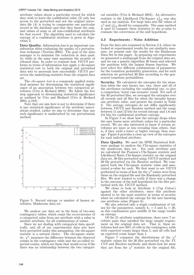
Figure 5: Record entropy vs number of known at-tributes, Mushroom data set.

We analyse our data set in the form of two-waycontingency tables, which count the co-occurrence ofa categorical value from one attribute with a value inanother attribute, for all combinations of values.

Since we are dealing with categorical data specif-ically, and all of our experimental data sets havebeen perturbed under this assumption, the chi-squarestatistic is a natural choice. The chi-square statis-tic, χ2, measures the difference between the observedcounts in the contingency table and the so-called ex-pected counts, which are those that would occur if thethere was no relationship between the two categori-

cal variables (Utts & Heckard 2004). An alternativestatistic is the Likelihood Chi-Square χ2

LR was alsoused in our analysis. For large data sets the values ofχ2 and χ2

LR should be comparable. The same methodis used to compare these statistics to the p-value toevaluate the correctness of the null hypothesis.

3.3 Experiments - Noise Addition

From the data sets examined in Section 2.3, where welooked at experimental results for our similarity mea-sure, we present only the results for the MushroomData Set in this paper. In preparing our experimentswe generated a multigraph from the original data set,and we ran a genetic algorithm 30 times and selectedthe partition with the largest fitness function. Wenext select five different combinations of parametersfor the transition probability generation, and for eachselection we perturbed 30 files according to the gen-erated transition probabilities.

Security. We calculated the entropies for the situa-tion when the user knows one, two, three and all ofthe attributes excluding the confidential one, to givea comparison ‘worst case scenario’ result. For each ofthe 30 perturbed files, we averaged the entropies overall records and all files for when the intruder knowsone attribute value, and present the results in Table3. The average entropies do not differ significantlybetween VICUS and Random method and the rangebetween 11 and 12 bits for record entropy and 1.6 and2.6 bits for confidential attribute entropy.

In Figure 5 we show how the entropy drops whenthe user learns more attribute values for a particularrecord. We are also interested to know if certain at-tributes are more or less revealing than others, thatis, if they yield a lower or higher entropy than aver-age. Figure 6 provides a close up view of the entropiesfor each individual attribute.

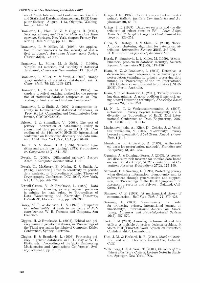
Data Quality. We used the SPSS Statistical Soft-ware package to analyse the Chi-square statistics ofthe mushroom data set. For each attribute pairwe calculated the Pearson’s Chi-Square statistic andLikelihood Ratio Chi-Square statistic on the originaldata set, 30 files perturbed using VICUS method and30 file perturbed via the Random method. We com-pared both the Chi-square statistic value and asso-ciated p-value for each. We first want to see VICUSperformed in terms of how far the χ2 values were fromthose on the original file and the Randomly perturbedfiles. We next wanted to verify if there was a changein the outcome of the null hypothesis for the files per-turbed with the VICUS method.

We chose to look at Attribute 4 (Cap Colour)against the other attributes, since this attributeshowed to be the most sensitive in terms of securitywhen we calculated the entropy for the user knowingone attribute value (Figure 6).

We also selected only a single combination of val-ues for the parameters, namely k1 = 5 and k2 = 20,as this combination gave middle of the range resultson entropy.

Of the 21 attribute combinations, there were 7 at-tribute pairs that satisfied the large sample require-ment on the original data set. That is, these at-tributes had over 80% of cells in the contingency tablewith expected counts larger than 5, and all cells hadan expected count larger than 1.

Figure 7 compares the distributions of the χ2

statistic values for the 30 files perturbed via the VI-CUS and Random methods, and shows how far awaythey are from the χ2 statistic for the original file,


146

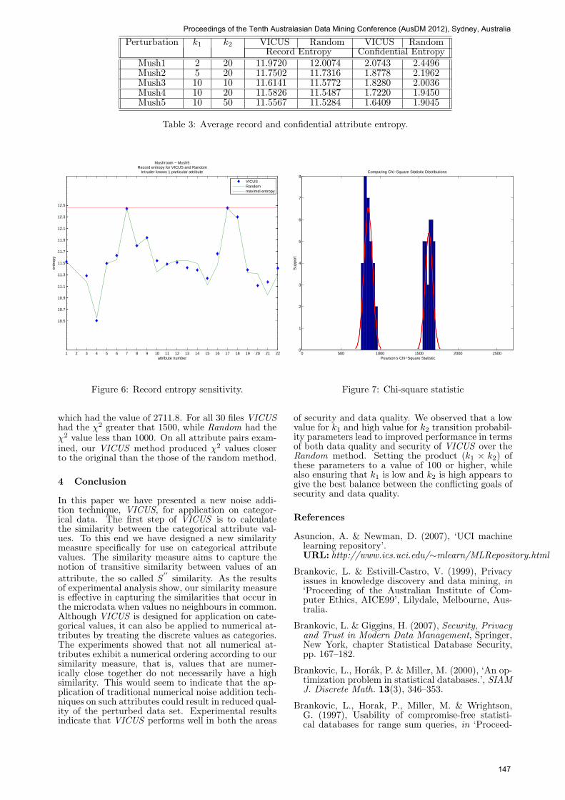
Perturbation k1 k2 VICUS Random VICUS RandomRecord Entropy Confidential Entropy

Mush1 2 20 11.9720 12.0074 2.0743 2.4496Mush2 5 20 11.7502 11.7316 1.8778 2.1962Mush3 10 10 11.6141 11.5772 1.8280 2.0036Mush4 10 20 11.5826 11.5487 1.7220 1.9450Mush5 10 50 11.5567 11.5284 1.6409 1.9045

Table 3: Average record and confidential attribute entropy.

1 2 3 4 5 6 7 8 9 10 11 12 13 14 15 16 17 18 19 20 21 22

10.5

10.7

10.9

11.1

11.3

11.5

11.7

11.9

12.1

12.3

12.5

Mushroom − Mush5Record entropy for VICUS and Random

Intruder knows 1 particular attribute

attribute number

entr

opy

VICUSRandommaximal entropy

Figure 6: Record entropy sensitivity.

which had the value of 2711.8. For all 30 files VICUShad the χ2 greater that 1500, while Random had theχ2 value less than 1000. On all attribute pairs exam-ined, our VICUS method produced χ2 values closerto the original than the those of the random method.

4 Conclusion

In this paper we have presented a new noise addi-tion technique, VICUS, for application on categor-ical data. The first step of VICUS is to calculatethe similarity between the categorical attribute val-ues. To this end we have designed a new similaritymeasure specifically for use on categorical attributevalues. The similarity measure aims to capture thenotion of transitive similarity between values of anattribute, the so called S

′′similarity. As the results

of experimental analysis show, our similarity measureis effective in capturing the similarities that occur inthe microdata when values no neighbours in common.Although VICUS is designed for application on cate-gorical values, it can also be applied to numerical at-tributes by treating the discrete values as categories.The experiments showed that not all numerical at-tributes exhibit a numerical ordering according to oursimilarity measure, that is, values that are numer-ically close together do not necessarily have a highsimilarity. This would seem to indicate that the ap-plication of traditional numerical noise addition tech-niques on such attributes could result in reduced qual-ity of the perturbed data set. Experimental resultsindicate that VICUS performs well in both the areas

0 500 1000 1500 2000 25000

1

2

3

4

5

6

7

8Comparing Chi−Square Statistic Distributions

Pearson’s Chi−Square Statistic

Sup

port

Figure 7: Chi-square statistic

of security and data quality. We observed that a lowvalue for k1 and high value for k2 transition probabil-ity parameters lead to improved performance in termsof both data quality and security of VICUS over theRandom method. Setting the product (k1 × k2) ofthese parameters to a value of 100 or higher, whilealso ensuring that k1 is low and k2 is high appears togive the best balance between the conflicting goals ofsecurity and data quality.

References

Asuncion, A. & Newman, D. (2007), ‘UCI machinelearning repository’.URL: http://www.ics.uci.edu/∼mlearn/MLRepository.html

Brankovic, L. & Estivill-Castro, V. (1999), Privacyissues in knowledge discovery and data mining, in‘Proceeding of the Australian Institute of Com-puter Ethics, AICE99’, Lilydale, Melbourne, Aus-tralia.

Brankovic, L. & Giggins, H. (2007), Security, Privacyand Trust in Modern Data Management, Springer,New York, chapter Statistical Database Security,pp. 167–182.

Brankovic, L., Horak, P. & Miller, M. (2000), ‘An op-timization problem in statistical databases.’, SIAMJ. Discrete Math. 13(3), 346–353.

Brankovic, L., Horak, P., Miller, M. & Wrightson,G. (1997), Usability of compromise-free statisti-cal databases for range sum queries, in ‘Proceed-


147

ing of Ninth International Conference on Scientificand Statistical Database Management, IEEE Com-puter Society’, August 11-13, Olympia, Washing-ton, pp. 144–154.

Brankovic, L., Islam, M. Z. & Giggins, H. (2007),Security, Privacy and Trust in Modern Data Man-agement, Springer, New York, chapter Privacy Pre-serving Data Mining, pp. 151–165.

Brankovic, L. & Miller, M. (1995), ‘An applica-tion of combinatorics to the security of statis-tical databases’, Australian Mathematical SocietyGazette 22(4), 173–177.

Brankovic, L., Miller, M. & Siran, J. (1996b),‘Graphs, 0-1 matrices, and usability of statisticaldatabases’, Congressus Numerantium 12, 196–182.

Brankovic, L., Miller, M. & Siran, J. (2002), ‘Rangequery usability of statistical databases’, Int. J.Comp. Math. 79(12), 1265–1271.

Brankovic, L., Miller, M. & Siran, J. (1996a), To-wards a practical auditing method for the preven-tion of statistical database compromise, in ‘Pro-ceeding of Australasian Database Conference’.

Brankovic, L. & Siran, J. (2002), 2-compromise us-ability in 1-dimensional statistical databases, in‘Proc. 8th Int. Computing and Combinatorics Con-ference, COCOON2002’.

Brickell, J. & Shmatikov, V. (2008), The cost ofprivacy: destruction of data-mining utility inanonymized data publishing, in ‘KDD ’08: Pro-ceeding of the 14th ACM SIGKDD internationalconference on Knowledge discovery and data min-ing’, ACM, New York, NY, USA, pp. 70–78.

Bui, T. N. & Moon, B. R. (1996), ‘Genetic algo-rithm and graph partitioning’, IEEE Transactionson Computers 45(7), 841–855.

Dwork, C. (2006), ‘Differential privacy’, LectureNotes in Computer Science 4052, 1–12.

Dwork, C., McSherry, F., Nissim, K. & Smith, A.(2006), Calibrating noise to sensitivity in privatedata analysis., in ‘Proceedings of Third Theory ofCryptography Conference, TCC 2006’, New York,NY, USA, pp. 265–284.

Estivill-Castro, V. & Brankovic, L. (1999), Dataswapping: Balancing privacy against precisionin mining for logic rules, in ‘Proceedings ofData Warehousing and Knowledge Discovery,DaWaK99’, Florence, Italy, pp. 389–398.

Garey, M. R. & Johnson, D. S. (1979), Computersand intractability: A guide to the theory of NP -completeness, W. H. Freeman and Company, SanFrancisco.

Giggins, H. & Brankovic, L. (2002), Ethical and pri-vacy issues in genetic databases, in ‘Proceedings ofthe Third Australian Institiute of Computer EthicsConference’, Sydney, Australia.

Giggins, H. & Brankovic, L. (2003), Protecting pri-vacy in genetic databases, in R. L. May & W. F.Blyth, eds, ‘Proceedings of the Sixth EngineeringMathematics and Applications Conference’, Syd-ney, Australia, pp. 73–78.

Griggs, J. R. (1997), ‘Concentrating subset sums at kpoints’, Bulletin Institute Combinatorics and Ap-plications 20, 65–74.

Griggs, J. R. (1999), ‘Database security and the dis-tribution of subset sums in Rm’, Janos BolyaiMath. Soc. 7, Graph Theory and Combinatorial Bi-ology pp. 223–252.

Guha, S., Rastogi, R. & Shim, K. (2000), ‘Rock:A robust clustering algorithm for categorical at-tributes’, Information Systems 25(5), 345–366.URL: citeseer.ist.psu.edu/guha00rock.html

Horak, P., Brankovic, L. & Miller, M. (1999), ‘A com-binatorial problem in database security’, DiscreteApplied Mathematics 91(1-3), 119–126.

Islam, M. Z. & Brankovic, L. (2005), Detective: Adecision tree based categorical value clustering andperturbation technique in privacy preserving datamining, in ‘Proceedings of the 3rd InternationalIEEE Conference on Industrial Informatics (INDIN2005)’, Perth, Australia.

Islam, M. Z. & Brankovic, L. (2011), ‘Privacy preserv-ing data mining: A noise addition framework us-ing a novel clustering technique’, Knowledge-BasedSystems 24, 1214–1223.

Li, N., Li, T. & Venkatasubramanian, S. (2007),t-closeness: Privacy beyond k-anonymity and l-diversity, in ‘Proceedings of IEEE 23rd Inter-national Conference on Data Engineering, 2007.ICDE 2007.’, pp. 106–115.

Machanavajjhala, A., Kifer, D., Gehrke, J. & Venki-tasubramaniam, M. (2007), ‘L-diversity: Privacybeyond k-anonymity’, ACM Trans. Knowl. Discov.Data 1(1), 3.

Muralidhar, K. & Sarathy, R. (2003), ‘A theoreti-cal basis for perturbation methods’, Statistics andComputing 13, 329–335.

Oganian, A. & Domingo-Ferrer, J. (2003), ‘A posteri-ori disclosure risk measure for tabular data basedon conditional entropy’, SORT - Statistics and Op-erations Research Transactions 27(2), 175–190.

Samarati, P. & Sweeney, L. (1998), Protecting privacywhen disclosing information: k-anonymity and itsenforcement through generalization and suppres-sion, in ‘Proceedings of the IEEE Symposium onResearch in Security and Privacy’, Oakland, Cali-fornia, USA.

Shannon, C. E. (1948), ‘A mathematical theory ofcommunication’, Bell Syst. Tech J. 27, 379–423.

Sweeney, L. (2002), ‘k-anonymity: a modelfor protecting privacy. international journal onuncertainty’, International Journal on Uncer-tainty, Fuzziness and Knowledge-based Systems10(5), 557–570.

Trottini, M. (2003), Assessing disclosure risk and datautility: A multiple objectives decision problem, in‘Joint ECE/Eurostat Work Session on StatisticalConfidentiality’, Luxembourg.

Utts, J. M. & Heckard, R. F. (2004), Mind on statis-tics, 2nd edn, Thomson-Brooks/Cole, Belmont,Calif.

Willenborg, L. & de Waal, T. (2001), Elements of Sta-tistical Disclosure Control, Lecture Notes in Statis-tics, Springer, New York, USA.


148

VICUS - A Noise Addition Technique for Categorical Data

Documents