VBF: Vector-Based Forwarding Protocol for Underwater Sensor …jcui/UWSN_papers/UCONN_CSE_UbiNet-TR05-… · 4 II. RELATED WORK In this section, we review some typical routing protocols

1

VBF: Vector-Based Forwarding Protocol for Underwater Sensor Networks

Peng Xie, Jun-Hong Cui, Li Lao

[email protected], [email protected], [email protected]

UCONN CSE Technical Report: UbiNet-TR05-03

Last Update: February 2006

Abstract

In this paper, we tackle one fundamental problem in Underwater Sensor Networks (UWSNs): robust, scalable

and energy efficient routing. UWSNs are significantly different from terrestrial sensor networks in the following

aspects: low bandwidth, high latency, node float mobility (resulting in high network dynamics), high error probability,

and 3-dimensional space. These new features bring many challenges to the network protocol design of UWSNs. In

this paper, we propose a novel routing protocol, called vector-based forwarding (VBF), aiming to provide robust,

scalable and energy efficient routing. VBF is essentially a location-based routing approach. No state information is

required on the sensor nodes and only a small fraction of the nodes are involved in routing. Moreover, packets are

forwarded in redundant and interleaved paths, which add robustness to VBF. Further, we develop a localized and

distributed self-adaptation algorithm, which helps to enhance the performance of VBF. The self-adaptation algorithm

allows the nodes to weigh the benefit to forward packets and reduce energy consumption by discarding the low

benefit packets. We evaluate the performance of VBF through extensive simulations. Our experiment results show

that for networks with small or medium node mobility (1 m/s-3 m/s), VBF can effectively accomplish the goals of

robustness, energy efficiency, and high success of data delivery.

I. INTRODUCTION

The Earth is a water planet. For decades, there have been significant interests in monitoring aquatic environments

for scientific exploration, commercial exploitation and coastline protection. Highly precise, real-time, and temporal-

spatial continuous aquatic environment monitoring systems are extremely important for various applications, such

as oceanographic data collection, pollution detection, and marine surveillance. However, traditional techniques, such

as remote telemetry and sequential local sensing, can not satisfy these high-demanding application requirements.

Recently, underwater sensor networks have emerged as a very powerful technique for many applications for

underwater environment, including monitoring, measurement, surveillance and control [24], [22], [21], [2], [8], [5],

[15]. Even though underwater sensor networks (UWSNs) share some common properties with terrestrial sensor

networks, such as the large number of nodes and limited power energy, UWSNs are significantly different from

terrestrial sensor networks in many aspects: low bandwidth, high latency, node float mobility (resulting in high

2

network dynamics), high error probability, and 3-dimensional space. These new features bring many challenges to

the protocol design of UWSNs. In this paper, we tackle one fundamental problem in UWSNs: robust, scalable and

energy efficient routing. In the following, we present the unique features of UWSNs and discuss how the routing

protocol design in UWSNs is challenged.

A. Unique Features of UWSNs

A UWSN is significantly different from any ground-based sensor network in terms of the following aspects:

• Low bandwidth and high latency in UWSNs. Acoustic channels (instead of RF channels) are used as the

communication method since radio does not work well in water. The propagation speed of acoustic signals

in water is about 1.5× 103 m/sec, which is five orders of magnitude lower than the radio propagation speed

(3×108 m/sec). Moreover, the available bandwidth of underwater acoustic channels is limited and dramatically

depends on both transmission range and frequency. According to [14], nearly no research and commercial

system can exceed 40 km× kbps as the maximum attainable Range× Rate product.

• UWSNs are highly dynamic. In a UWSN1, the majority of sensor nodes, except some fixed nodes equipped

on surface-level buoys, have low or medium mobility due to water current and other underwater activities.

From empirical observations, underwater objects may move at the speed of 2-3 knots (or 3-6 kilometers per

hour) in a typical underwater condition. This kind of node mobility results in an unstable neighborhood for a

node in the network, which is a big challenge for routing protocol design.

• UWSNs are highly error-prone. Underwater acoustic communication channels are affected by many factors

such as path loss, noise, multi-path, and Doppler spread. All these factors cause high bit-error and delay

variance. Thus, communication links in UWSNs are highly error-prone. Moreover, sensor nodes are more

vulnerable in harsh underwater environments. Compared with their counterparts on land, underwater sensor

networks have a higher node-failure rate.

• UWSNs are 3-dimensional. UWSNs are usually deployed in a 3-dimensional space. This is different from

the 2-dimensional deployment of most land-based sensor networks.

These characteristics of UWSNs make the existing work for terrestrial sensor networks unsuitable for UWSNs

and bring up many challenges for almost every level of the protocol suite.

B. Routing Challenges in UWSNs

Same as in terrestrial sensor networks, saving energy is a major concern in UWSNs. At the same time, UWSN

routing should be able to handle node mobility. This requirement makes most existing energy-efficient routing

protocols unsuitable for UWSNs. There are many routing protocols proposed for terrestrial sensor networks, such

as Directed Diffusion [11], and TTDD (Two-Tier Data Dissemination) [25]. These protocols are mainly designed

1In this paper, we target a mobile UWSN (where most sensors are not fixed, and they can float with water current). This type of UWSNs

are very useful in many applications, such as estuary dynamic monitoring and submarine detection [5], [15]

3

for stationary networks. They usually employ query flooding as a powerful method to discover data delivery paths.

In UWSNs, however, most sensor nodes are mobile, and the “network topology” changes very rapidly even with

small displacements. The frequent maintenance and recovery of forwarding paths is very expensive in high dynamic

networks, and even more expensive in dense 3-dimensional UWSNs.

The multi-hop routing protocols in terrestrial mobile ad hoc networks fall into two categories: proactive routing

and reactive routing (aka., on-demand routing). In proactive ad hoc routing protocols like OLSR [1], TBRPF [18]

and DSDV [19], the cost of proactive neighbor detection could be very expensive because of the large scale of

UWSNs. On the other hand, in on-demand routing (with AODV [20] and DSR [12] as common examples), routing

operation is triggered by the communication demand at sources. In the phase of route discovery, the source seeks

to establish a route towards the destination by flooding a route request message, which would be very costly in

large scale UWSNs.

Thus, to provide scalable and efficient routing in UWSNs, we have to seek for new solutions. In this paper,

we investigate this challenging routing problem in UWSNs, with scalability and energy efficiency as the design

objectives. Moreover, robustness is also an important concern due to the high node failure rate and error-prone

channels in UWSNs.

C. Contributions

We propose a novel routing protocol, called vector-based forwarding (VBF), to address the routing problem

in UWSNs. VBF is essentially an integration of localization and routing in that the localization and routing are

performed at the same time. VBF is robust, scalable and energy efficient. In essence, VBF is a geographic routing

approach. No state information is required on the sensor nodes and only a small fraction of the nodes are involved

in routing. Moreover, in VBF, packets are forwarded along redundant and interleaved paths from a source to

a destination, it is robust against packet loss and node failure. Further, we develop a localized and distributed

self-adaptation algorithm to enhance the performance of VBF. The self-adaptation algorithm allows the nodes to

weigh the benefit to forward packets and reduce energy consumption by discarding low benefit packets. We also

give a formal analysis of the self-adaptation algorithm. We evaluate the performance of VBF through extensive

simulations. Our experiment results show that for networks with small or medium node mobility (1 m/s-3 m/s),

VBF can effectively achieve the goals of robustness, energy efficiency, and high success of data delivery.

The rest of this paper is organized as follows. We first briefly review some related works and discuss their

applicability to UWSNs in Section II. Then, we present our VBF protocol in Section III. After that, we analyze

and evaluate VBF in Section IV and Section V respectively. Finally, we conclude the paper and layout some future

work in Section VI.

4

II. RELATED WORK

In this section, we review some typical routing protocols in terrestrial sensor networks and mobile ad hoc

networks. We also discuss a closely related generic routing protocol, TBF [17].

A. Routing in Terrestrial Sensor Networks

In last few years, many energy efficient routing protocols have been proposed for terrestrial sensor networks,

such as Directed Diffusion [11], Two-Tier Data Dissemination[25], GRAdient[26], Rumor routing [4], and SPIN

[9]. In the following, we brief these protocols and discuss why they are not suitable for the underwater sensor

network environments.

Directed Diffusion is proposed in [11]. In the target application scenario, the sink floods its interest into the

network, and the source node responds with data. The data are first forwarded to the sink along all possible paths.

Then, an optimal path is enforced from the sink to the source recursively based on the quality of the received data.

Directed Diffusion works well in low dynamic networks, where most nodes are stationary and forwarding paths are

relatively stable. However, if we apply Directed Diffusion in UWSNs, it will consume a large amount of resource

(including energy) to maintain the forwarding paths due to node mobility.

In the Rumor routing algorithm [4], both event notifications and data queries are forwarded randomly. The

successful data delivery depends on the chance that these two types of forwarding paths interleave. In stationary

networks, it is most likely that these paths will meet since they are relatively stable. However, in underwater sensor

networks, this is unlikely to happen. Even in networks with low mobility, the instability of forwarding paths is

worsen by the low propagation speed of acoustic signals.

SPIN (Sensor Protocol Information via Negotiation) is proposed for low data rate networks [9]. When a node

wants to send data, it broadcasts a description message of the data, and each neighbor decides whether to accept the

data based on its local resource condition. Once again, the high propagation delay in UWSNs makes this protocol’s

throughput low. Moreover, flooding in SPIN depletes the energy of the network, especially for medium or high

data rate networks.

TTDD (Two-Tier Data Dissemination) addresses the problem caused by mobile sinks [25]. In this protocol, the

source sensor initiates the process to construct a grid covering the whole field. Data and queries are forwarded

along the cross points in the grid. The impact of the sink mobility is confined within each cell. When most nodes

in the network are fixed, it costs less energy to maintain the grid. However, the overhead to maintain the grid will

increase significantly when most nodes are mobile (for example, in UWSNs).

GRAdient broadcast is a robust data delivery protocol proposed in [26]. In GRAdient, a cost field is built in the

whole network by the sink, which has the lowest cost. Data packets are forwarded along the direction from higher

cost nodes to lower cost nodes. The width of the path is controlled by the credits of each packet. In this way,

GRAdient improves robustness. However, in UWSNs where sensor nodes are mobile, the protocol will consume a

5

large amount of scarce energy to update the cost field in order to keep relatively accurate paths from the source to

the sink.

In short, the routing protocols for UWSNs have to address the node mobility issue at minimum energy expenditure.

However, existing routing protocols designed for terrestrial sensor networks can not satisfy this requirement. When

applied directly in the underwater sensor network environments, these proposals become very expensive in terms

of energy due to node mobility.

B. Geographic Routing Protocols for Mobile Ad Hoc Networks

In the literature, there are many geographic routing protocols [3], [13], [10], [6], [27], [7], [23], [16] proposed to

address the node mobility issue. In these protocol, location information of nodes is used to determine the forwarding

route. VBF is essentially also a geographic routing protocol. Compared with VBF, these protocols assume that the

location service (i.e., positioning the nodes) is available. Thus, they do not address how to position nodes in a

highly dynamic network, which in fact is the foundation of the VBF protocol. Moreover, in order to save energy,

VBF adopts a self-adaptation algorithm to allow nodes to weigh the benefit of forwarding packets. This idea shares

some similarity with the timer-based contention algorithm in CBF protocol [6]. The major differences between

these two algorithms are two-fold: (1) the timer-based contention algorithm is designed for 2-dimensional space,

not for 3-dimensional networks; (2) the timer-based contention algorithm can not suppress the duplicate packets

from nodes close to the optimal position.

C. Trajectory-Based Forwarding (TBF)

Trajectory-Based Forwarding (TBF) proposed in [17] is a generalization of source routing and Cartesian for-

warding in ad-hoc networks. Source routing relieves the nodes en-route of the burden of maintaining routing state.

In TBF, the forwarding path is specified as a trajectory carried in data packets. The trajectory can be represented

as either a function or an equation. The idea of TBF looks promising for large scale sensor networks, since it

neither involves query flooding nor employs route discovery and maintenance. However, some problems have to be

addressed when applying it in underwater sensor networks. First of all, the trajectory-related computation is usually

expensive. Second, the overhead of representing trajectory is usually very high. Furthermore, the applicability of

TBF in mobile network environments is yet to be investigated.

In this work, we propose VBF, a much more simplified version of TBF. In VBF, the path is specified by a vector

(referred to as routing vector in this paper), a extremely simplified trajectory. Therefore, no extra overhead is

needed to represent the complex trajectory. The simple vector-related calculations can be done quickly. Moreover,

we propose a self-adaption algorithm that enables each node to weigh the benefit of forwarding a packet and decide

whether to forward the packet just based on local information, thus, saving energy.

III. VECTOR-BASED FORWARDING PROTOCOL (VBF)

In this section, we present our vector-based forwarding (VBF) protocol.

6

A. Overview of VBF

In sensor networks, energy constraint is a crucial factor since sensor nodes usually run on battery, and it is

impossible or difficult to recharge them in most application scenarios. In underwater sensor networks, in addition

to energy saving, the routing algorithms should be able to handle node mobility in an efficient way.

Vector-Based Forwarding (VBF) protocol meets these requirements successfully. In VBF, each packet carries the

positions of the sender, the target and the forwarder (i.e., the node which transmits this packet). The forwarding

path is specified by the routing vector from the sender to the target. Upon receiving a packet, a node computes

its relative position to the forwarder by measuring its distance to the forwarder and the angle of arrival (AOA)

of the signal2. Recursively, all the nodes receiving the packet compute their positions. If a node determines that

it is close to the routing vector enough (e.g., less than a predefined distance threshold), it puts its own computed

position in the packet and continues forwarding the packet; otherwise, it simply discards the packet. In this way,

all the packet forwarders in the sensor network form a “routing pipe”: the sensor nodes in this pipe are eligible for

packet forwarding, and those which are not close to the routing vector (i.e., the axis of the pipe) do not forward.

Fig. 1 illustrates the basic idea of VBF. In the figure, node S1 is the source, and node S0 is the sink. The routing

vector is specified by−−→S1S0. Data packets are forwarded from S1 to S0. Forwarders along the routing vector form

a routing pipe with a pre-controlled radius (i.e., the distance threshold, denoted by W in this paper).

S1S1

Not close to the vector => No Forward

WW

S0S0

Fig. 1. A high-level view of VBF for UWSNs

As we can see, like all other source routing protocols, VBF requires no state information at each node. Therefore,

it is scalable to the size of the network. Moreover, in VBF, only the nodes along the forwarding path (specified by

the routing vector) are involved in packet routing, thus saving the energy of the network.

2We assume that sensor nodes in UWSNs are armed with some devices that can measure the distance and the angle of arrival (AOA) of

the signal. This assumption is justified by the fact that acoustic directional antennae are of much smaller size than RF directional antennae

due to the extremely small wavelength of sound. Moreover, underwater sensor nodes are usually larger than land-based sensors, and they

have room for such devices.

7

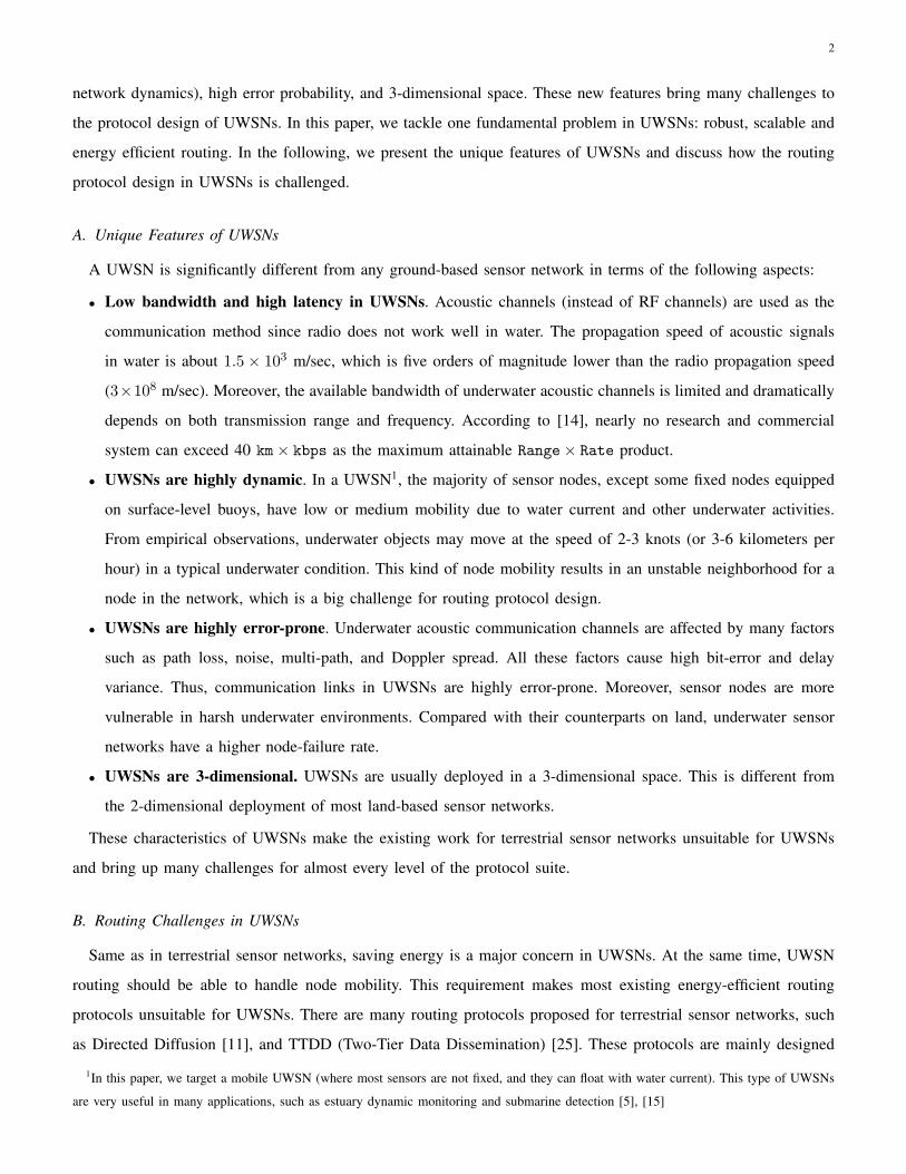
B. The Basic VBF Protocol

VBF is a source routing protocol. Each packet carries simple routing information. In a packet, there are three

position fields, OP, TP and FP, i.e., the coordinates of the sender, the target and the forwarder. In order to handle

node mobility, each packet contains a RANGE field. When a packet reaches the area specified by its TP, this packet

is flooded in an area controlled by the RANGE field. The forwarding path is specified by the routing vector from

the sender to the target. Each packet also has a RADIUS field, which is a pre-defined threshold used by sensor

nodes to determine if they are close enough to the routing vector and eligible for packet forwarding.

There are two types of queries. One is location-dependent query. In this case, the sink is interested in some

specific area and knows the location of the area. The other type is location independent query, when the sink wants

to know some specific type of data regardless of its location. For example, the sink wants to know if there exist

abnormal high temperatures in the network. Both of these two types of queries can be routed effectively by VBF.

1. Query Forwarding For location dependent queries, the sink is interested in some specific area, so it issues

an INTEREST query packet, which carries the coordinates of the sink and the target in the sink-based coordinate

system. Each node which receives this packet calculates its own position and the distance to the routing vector. If

the distance is less than RADIUS (i.e., the distance threshold), then this node updates the FP field of the packet and

forwards it; otherwise, it discards this packet. For location-dependent queries, the INTEREST packet may carry

some invalid positions for the target. Upon receiving such packets, a node first checks if it has the data which

the sink is interested in. If so, the node computes its position in the sink-based coordinate system, generates data

packets and sends back to the sink. Otherwise, it updates the FP field of the packet and further forwards it.

2. Source initiated Query In some application scenarios, the source can initiate the query process. VBF also

supports such source initiated query. If a source senses some events and wants to inform the sink, it first broadcasts

a DATA READY packet. Upon receiving such packets, each node computes its own position in the source-based

coordinate system, updates the FP field and forwards the packet. Once the sink receives this packet, it calculates

its position in the source-based coordinate system and transforms the position of the source into its own coordinate

system. Then the sink can decide if it is interested in such data. If so, it may send out an INTEREST packet to

the area where the source resides.

Handling Source Mobility Since the source node keeps moving, its location calculated based on the old INTEREST

packet might not be accurate any more. If no measure is taken to correct the source location, the actual forwarding

path might get far away from the expected one, i.e., the destination of the data forwarding path most probably

misses the sink. We propose the following sink-assisted approach to solve this problem.

The source keeps sending packets to the sink, and the sink can utilize the source location information carried

in the packets to determine if the source moves out of the targeted scope. For example, if the sink calculates its

8

Sink (S 0 )

Source (S 1 )

F

W

W

p d

R

A

Sink (S 0 )

Source (S 1 )

F

W

W

p d

R

A

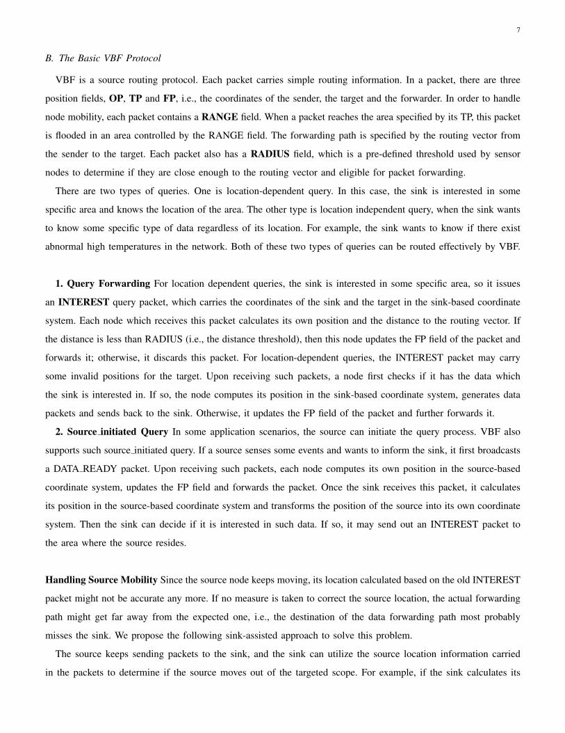
Fig. 2. Desirableness Factor

1 1

Sink (S 0 )

Source (S )

F A

D

B

W

W

Sink (S 0 )

Source (S )

F A

D

B

W

W

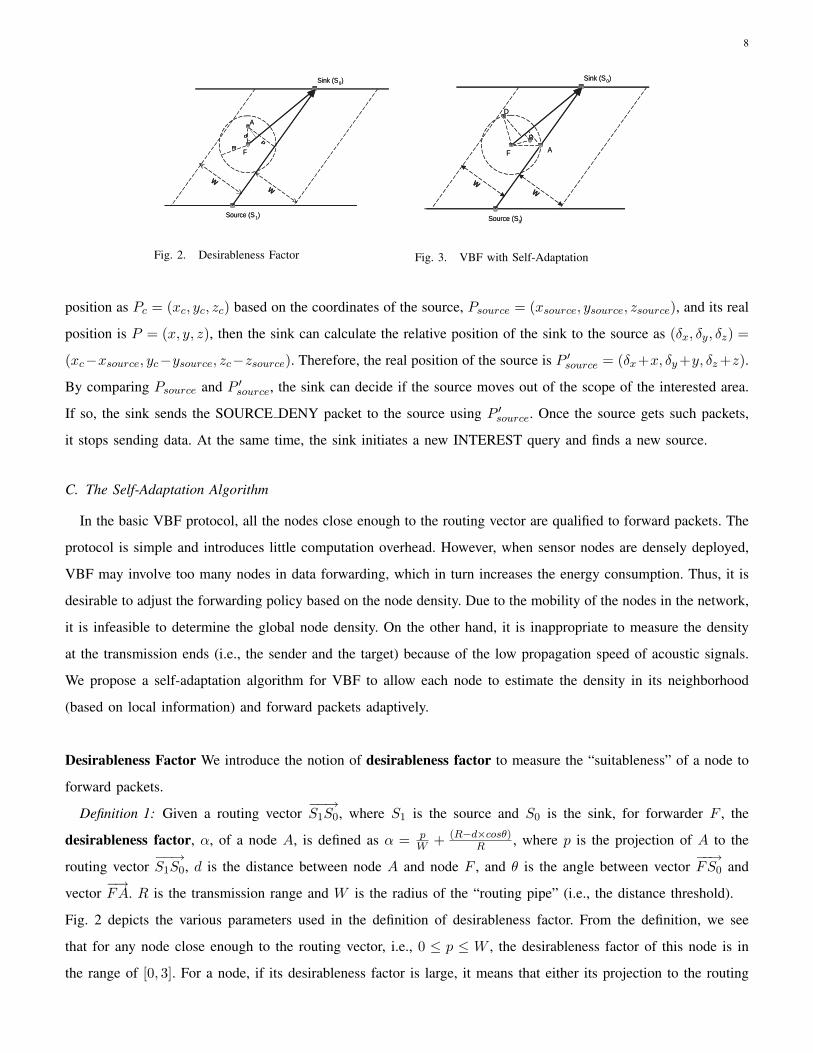
Fig. 3. VBF with Self-Adaptation

position as Pc = (xc, yc, zc) based on the coordinates of the source, Psource = (xsource, ysource, zsource), and its real

position is P = (x, y, z), then the sink can calculate the relative position of the sink to the source as (δx, δy, δz) =

(xc−xsource, yc−ysource, zc−zsource). Therefore, the real position of the source is P ′source = (δx+x, δy +y, δz +z).

By comparing Psource and P ′source, the sink can decide if the source moves out of the scope of the interested area.

If so, the sink sends the SOURCE DENY packet to the source using P ′source. Once the source gets such packets,

it stops sending data. At the same time, the sink initiates a new INTEREST query and finds a new source.

C. The Self-Adaptation Algorithm

In the basic VBF protocol, all the nodes close enough to the routing vector are qualified to forward packets. The

protocol is simple and introduces little computation overhead. However, when sensor nodes are densely deployed,

VBF may involve too many nodes in data forwarding, which in turn increases the energy consumption. Thus, it is

desirable to adjust the forwarding policy based on the node density. Due to the mobility of the nodes in the network,

it is infeasible to determine the global node density. On the other hand, it is inappropriate to measure the density

at the transmission ends (i.e., the sender and the target) because of the low propagation speed of acoustic signals.

We propose a self-adaptation algorithm for VBF to allow each node to estimate the density in its neighborhood

(based on local information) and forward packets adaptively.

Desirableness Factor We introduce the notion of desirableness factor to measure the “suitableness” of a node to

forward packets.

Definition 1: Given a routing vector−−→S1S0, where S1 is the source and S0 is the sink, for forwarder F , the

desirableness factor, α, of a node A, is defined as α = pW + (R−d×cosθ)

R , where p is the projection of A to the

routing vector−−→S1S0, d is the distance between node A and node F , and θ is the angle between vector

−−→FS0 and

vector−→FA. R is the transmission range and W is the radius of the “routing pipe” (i.e., the distance threshold).

Fig. 2 depicts the various parameters used in the definition of desirableness factor. From the definition, we see

that for any node close enough to the routing vector, i.e., 0 ≤ p ≤ W , the desirableness factor of this node is in

the range of [0, 3]. For a node, if its desirableness factor is large, it means that either its projection to the routing

9

vector is large or it is not far away from the forwarder. In other words, it is not desirable for this node to continue

forwarding the packet. On the other hand, if the desirableness factor of a node is 0, then this node is on both the

routing vector and the edge of the transmission range of the forwarder. We call this node as the optimal node, and

its position as the best position. For any forwarder, there is at most one optimal node and one best position. If the

desirableness factor of a node is close to 0, it means this node is close to the best position.

The Algorithm We propose a self-adaptation algorithm based on the concept of desirableness factor. This algorithm

aims to select the most desirable nodes as forwarders. In this algorithm, when a node receives a packet, it first

determines if it is close enough to the routing vector. If yes, the node then holds the packet for a time period

related to its desirableness factor. In other words, each qualified node delays forwarding the packet by a time

interval Tadaptation, which is calculated as follows:

Tadaptation =√

α× Tdelay +R− d

v0, (1)

where Tdelay is a pre-defined maximum delay, v0 is the propagation speed of acoustic signals in water, i.e., 1500m/s,

and d is the distance between this node and the forwarder. In the equation, the first term reflects the waiting time

based on the node’s desirableness factor: the more desirable (i.e., the smaller the desirableness factor), the less time

to wait. The second term represents the additional time needed for all the nodes in the forwarder’s transmission

range to receive the acoustic signal from the forwarder.

During the delayed time period Tadaptation, if a node receives duplicate packets from n other nodes, then this

node has to compute its desirableness factors relative to these nodes, α1, . . . , αn, and the original forwarder, α0. If

min(α0, α1, . . . , αn) < αc/2n, where αc is a pre-defined initial value of desirableness factor (0 ≤ αc ≤ 3), then

this node forwards the packet; otherwise, it discards the packet.

Analysis Essentially, the above self-adaptation algorithm gives higher priority to the desirable node to continue

broadcasting the packet, and it also allows a less desirable node to have chances to re-evaluate its “importance”

in the neighborhood. After receiving the same packets from its neighbors, the less desirable node can measure its

importance by computing its desirableness factor relative to its neighbors. If there are many more desirable nodes in

the neighborhood, we exponentially reduce the probability of this node to forward the packet. That is, it is useless

for this node to forward the packet anymore since many other more desirable nodes have forwarded the packet. In

fact, if a node receives more than two duplicate packets during its waiting time, it is most likely that this node will

not forward the packet no matter what initial value αc takes. In this way, we can reduce the computation overhead

by skipping the re-evaluation of the desirableness factor.

From Equation 1, we can see that the optimal node does not defer forwarding packets in the self-adaptation

algorithm. Thus, we have the following lemma.

Lemma 1: If there exists an optimal path from the sender to the target, i.e., each node in the path is the optimal

10

node for its upstream node, then the self-adaptation algorithm selects this path and entails no delay.

An Example We illustrate VBF with self-adaptation in Fig. 3. In this figure, the forwarding path is specified as

the routing vector−−→S1S0 from the source S1 to the sink S0. The node F is the current forwarder. There are three

nodes namely, A, B and D in its transmission range. Node A has the smallest desirableness factor among these

nodes. Therefore, A has the shortest delay time and sends out the packet first. As shown in this figure, node B is

most likely to discard the packet because it is in the transmission range of A and it has to re-evaluate the benefit

to send the packet. Node D is out of the transmission range of A; therefore, it also forwards the packet.

D. Summary

We have described the basic VBF routing protocol and the self-adaptation algorithm. We can see that VBF

addresses the mobility of nodes in the network effectively. The positioning of nodes is performed locally and no

global synchronization required. VBF has no requirement for stable forward path. VBF is an energy efficient and

scalable protocol. 1) In VBF, no state information is required for each node; therefore, it is scalable to the size of

the network; 2) In VBF, only the nodes close to the routing vector are involved in packet forwarding, and all other

nodes are in idle state, thus saving energy. The self-adaptation algorithm helps to further reduce energy consumption

by selecting more desirable nodes.

VBF is also robust and less computationally demanding. 1) The success of data delivery is not dependent on

the stable neighborhood, but on the node density. If there exists at least one path in the “routing pipe” specified

by the routing vector, then the packet can be successfully delivered; 2) The computation demand on each node is

appropriate for routing on-demand since only simple vector-related calculation is needed.

IV. THEORETICAL ANALYSIS

A. The Robustness of VBF

VBF is robust against packet loss and node failure in that it uses redundant paths to forward the data packets.

Some of these paths are interleaved and some are parallel, as are determined by the deployment of nodes. In this

subsection, we estimate the successful delivery probability of a packet in a simple case.

We use R to denote the transmission range and W to denote the routing pipe radius. We also assume that all the

nodes are deployed in layers, and the adjacent layers are parted by R2 . The routing pipe is a cylinder from source

to the sink dimensioned by W and R. All the nodes inside the routing pipe are qualified forwarders. We use d to

denote the density of nodes, pl to denote the loss probability of packets and pe to denote the failure probability of

nodes. We use h to denote the number of hops (or layers). Since there are h layers in the cylinder, the number of

nodes in each layer is estimated as Nl = π×W 2×R×d2 . Therefore, the number of normal (i.e., functioning) nodes at

each layer are Nl × (1 − pe). The transmission space of a node is a sphere centered at this node with radius R.

When this node transmits a packet, all the nodes inside the sphere can hear that packet. There are three layers of

nodes inside the sphere. We estimate the number of nodes in each layer as nt = 43 × πR3 × d× 1

3 .

11

For a normal sender, the probability that its packet is received by the nodes in the upper layer is estimated as

P1 = 1− (1− (1− pl)(1− pe))nt . (2)

The transmission fails only if all of its upper layer neighbors fail or the packet is lost in all the links to these

neighbors. Then the probability that a packet is transmitted successfully from the lower layer to the upper layer is

estimated as

PL = 1− (1− P1)Nl×(1−pe). (3)

Therefore, the probability of successful delivery of one packet for h is calculated as

P = P hL . (4)

Here, we assume that for one layer, if one node receives a packet, all the normal nodes will eventually receive the

packet. This assumption is justified by the fact that all the normal nodes can receive data packets from the nodes

in the lower layer or from the nodes in the same layer. This assumption indicates the independence between layers.

Combining Equation 2, 3 and 4, we can easily see that when node density d increases, the probability that a

packet is forwarded h hops successfully approaches 1 dramatically. We can also observe that VBF is robust against

both link failure and node failure. For example, if d = 1/1000node/m3, the radius and transmission range are both

20 meters. Then the average number of nodes in the range of the sender is about 17, about one-third of which are

valid forwarders, i.e., 5 nodes will forward the packets. In such network setting, if we assume that packet loss is 0,

when the node failure is 65%, the probability that a packet is forwarded 20 hops successfully is 90%. On the other

hand, if we assume the node failure is 0, when the packet loss is 77%, the probability that a packet is forwarded

20 hops successfully is 90%. We will further evaluate the robustness of VBF using simulations in Section V.

B. The Lower Bound for Tdelay

The self-adaptation algorithm in VBF introduces extra delay in data forwarding. The purpose of the delay is to

differentiate the importance of the nodes in the transmission range of a forwarder. Intuitively, if we set a smaller

maximum delay, Tdelay, we can reduce the end-to-end delay. However, due to the purpose of the delay time used

by VBF, Tdelay must be set large enough. We give the lower bound for Tdelay in this section.

Let N be the total number of nodes in the network and the space be X × Y × Z. Then the average distance

among the nodes is given by d =√

∆x2 + ∆y2 + ∆z2, where ∆x = XN ,∆y = Y

N and ∆z = ZN . Let W be

the radius of the routing pipe and R be the transmission range. The average time for an acoustic signal to travel

between two neighbor nodes is T = dv0

, where v0 is the propagation speed of acoustic signals in water. The delay

time Tadapation in the self-adaptation algorithm should be greater than T . Let D = min{W,R}, and ∆α be the

difference of the desirableness factors of these two nodes. It is easy to get ∆α ≤ 2× dD . Therefore, we obtain the

following lemma.

Lemma 2: The lower bound for Tdelay is√

Dd√2×V

.

12

Even though the distance between the neighbor nodes is not always exactly equal to the average distance, the

probability that the distance, d, between two adjacent nodes deviates from the average distance, d, is bounded by

Pr[d ≤ (1− δ)d] ≤ e−dδ2

2 . (5)

That is, the probability that there is a large difference between d and d is very small. It justifies the lower bound

for Tdelay. In other words, it is useless to set Tdelay smaller than√

Dd√2V

in the self-adaptation algorithm.

C. Distinguishing Two Adjacent Nodes

In the self-adaptation algorithm, we want to distinguish the importance of two adjacent nodes. For a forwarder,

if the desirableness factors of these two nodes approach 0, then these nodes are close to the best position of the

forwarder. This implies that these nodes are close to each other, and most of their transmission spaces overlap;

thus, the benefit for both nodes to forward the packet is not justified. The self-adaptation algorithm attempts to

differentiate the delay time of these nodes to the extent such that the difference between their delay time periods is

large enough to allow the optimal node to suppress the other node. If the difference of their desirableness factors

is very small, we want such small difference to cause the difference of their delay times as large as possible.

Theoretically, we want lim∆→0∆Tadaptation(α)

∆α → ∞. Let T (α) = C × αK be the delay time function of the

desirableness factor. We get∂T (α)

∂α= C ×KαK−1. (6)

It is easy to see that if K < 1, limα→0∂T (α)

∂α → ∞. Therefore, for our purpose, any 0 < K < 1 satisfies our

purpose. In our algorithm, we set K = 1/2 (please refer to Equation 1). When we set the delay time for a node

proportional to the square root of the desirableness factor, we actually distinguish the nodes with slightly different

desirableness factors by a smaller Tdelay, thus, decreasing the end-to-end delay.

V. PERFORMANCE EVALUATION

In this section, we evaluate the performance of VBF through extensive simulations in NS-2. We first brief our

implementation of MAC protocol, then define the performance metrics and describe the simulation methodology.

We evaluate how network parameters such as node density, node mobility, and routing pipe radius, affect the

performance of VBF.

A. Implementation of MAC Protocol

VBF is a routing protocol, and medium access is not its concern. However, its performance can be significantly

affected by the underlying MAC protocol. Since the whole area of UWSNs is too young, there is no standard MAC

protocol yet. To evaluate the performance of VBF, we implement a simple MAC protocol based on CSMA. In this

MAC protocol, only broadcast is supported. When a sender has packets to send, it first senses the channel. If the

13

channel is free, it broadcasts its packets. If the channel is busy, it uses a back-off algorithm to contend the channel.

The maximum number of back-offs is 4. In this protocol, there is no collision detection, no RTS/CTS, and no ACK.

In our experiments, we measure packet delivery ratio, energy consumption and end-to-end delay achieved by

VBF. We admit that these metrics can be dramatically impacted by the underlying MAC protocol. On the one hand,

we only use the results for comparison purpose. One the other hand, we try to eliminate the effect of underlying

protocols as much as we can. In order to avoid packet transmission interference, we limit the sending rate to 2

packets per second, which is low enough to avoid interference caused by two continuous packets. In order to reduce

the collision and interference among neighbor nodes, each sender randomly delays its sending time in VBF.

The data rate for MAC protocol is set to 500 kbps, and the propagation speed of acoustic signals is set 1500

m/s [14].

B. Metrics and Methodology

Metrics We define three metrics to quantify the performance of VBF: success rate, energy consumption and

average delay. The success rate is the ratio of the number of packets successfully received by the sink to the

number of packets generated by the source. The communication time is the total time spent in communication of

sensor networks in the simulation including transmission time and receiving time of all nodes in networks3. The

average delay is the average end-to-end delay for each packet received by the sink. Even though the actual average

delay is determined by many factors such as medium contention, collision detection and avoidance (which we do

not address in this paper) and absolute values are not very meaningful, it is useful metric to evaluate a routing

protocol when a comparison is performed.

Experimental Methodology In our simulations, sensor nodes are deployed uniformly in a space of 100×100×100.

They can move in horizontal two-dimensional space, i.e., in the X-Y plane (which is the most common mobility

pattern in underwater applications). The transmission range is set to 20 meters. In order to have a bigger number

of hops, the source and the sink are fixed at (90,90,100) and (10,10,0), respectively. All other nodes in the network

are mobile with the same movement pattern unless specified otherwise. Each node randomly selects a destination

and moves toward that destination. Once the node arrives at the destination, it randomly selects a new destination

and moves in a new direction. The source sends data packets at the rate of 2 packets per second. The data packet

size is 76 bytes and control packet is 32 bytes. The total simulation time is 200 seconds.

C. Impact of Density and Mobility

We first investigate the impact of node density and mobility. In this set of experiments, all the mobile nodes

have the same speed. The routing pipe radius is fixed at 20 meters. We vary the mobility speed of each node from

3Since the energy consumption on communication is determined by many factors such as the implementation of hardware, sleep control,

and MAC protocols, we use communication time to evaluate the energy consumption.

14

0 1

2 3

4 5

Speed of nodes 600

800

1000

1200

1400

Number of nodes

0.5 0.55 0.6

0.65 0.7

0.75 0.8

0.85 0.9

0.95 1

Success rate (%)

Fig. 4. Impact of density & mobility on success

rate

0 1

2 3

4 5

Speed of nodes 600

800

1000

1200

1400

Number of nodes

0

100

200

300

400

500

600

Communication time (second)

Fig. 5. Impact of density & mobility on commu-

nication time

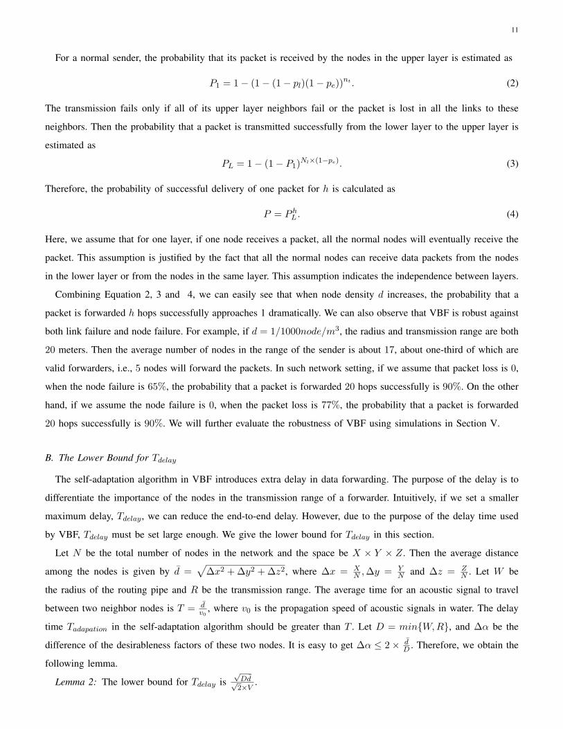
0 m/s to 5 m/s and the number of nodes from 500 to 1500. The simulation results are plotted in the Fig. 4, Fig. 5

and Fig. 6.

Fig. 4 shows the success rate as the function of the number of nodes and the speed of nodes. When the node

density is low, the success rate increases with density. However, when more than 1100 nodes are deployed in the

space, the success rate remains above 95%. The success rate decreases slightly when the nodes are mobile, however,

it is rather stable under different mobility speeds.

Fig. 5 depicts the communication time as the number of nodes and the speed of nodes vary. The communication

time increases when the number of nodes increases since more nodes are involved in packet forwarding. For the

same number of nodes in the network, this figure also shows that the communication time in static networks is

slightly less than that in dynamic networks. However, the communication time remains relatively stable as we vary

the mobility speed of nodes in the network.

As shown in Fig. 6, the average delay decreases as there are more nodes in the network. This trend is attributed

to the self-adaptation algorithm. When the number of nodes increases, the path from the sender to the receiver,

selected by the self-adaptation algorithm, are closer to the optimal path; therefore, the end-to-end delay decreases.

In contrast, the average delay remains almost the same as we vary the speed of nodes while keeping the number

of nodes fixed.

This set of simulation experiments have shown that in VBF, node speed has little impact on success rate, energy

consumption and average delay. It demonstrates that VBF could handle node mobility very effectively.

D. Impact of the Routing Pipe Radius

We test the impact of the routing pipe radius (i.e., the distance threshold) in this set of simulations. There are

500 nodes in the network, and their speed is fixed at 3m/s. We vary the radius from 0 meters to 50 meters. We

also implement a naive flooding protocol, which serves as upper or lower bounds for various performance metrics.

The results are shown in Fig. 7, and Fig. 8 and Fig. 9.

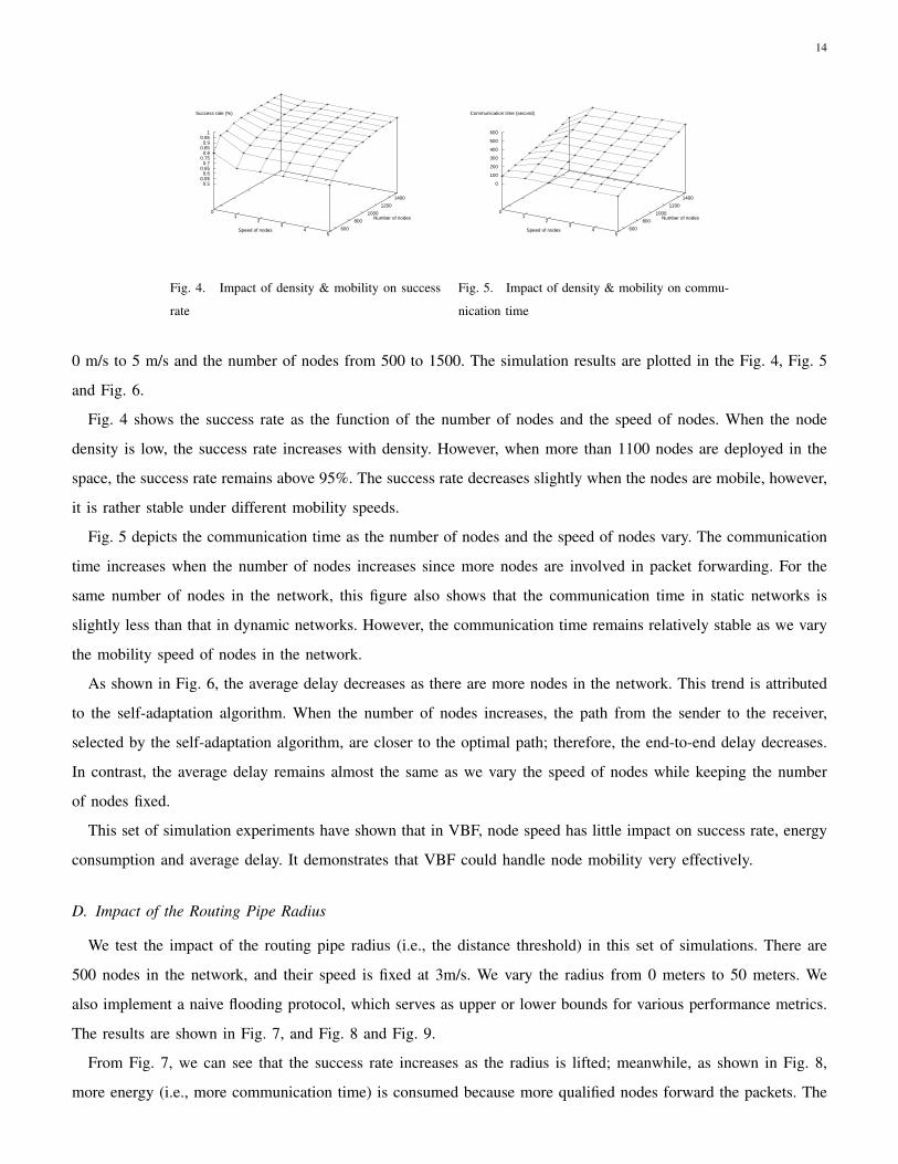
From Fig. 7, we can see that the success rate increases as the radius is lifted; meanwhile, as shown in Fig. 8,

more energy (i.e., more communication time) is consumed because more qualified nodes forward the packets. The

15

0 1

2 3

4 5

Speed of nodes 600

800

1000

1200

1400

Number of nodes

1

1.2

1.4

1.6

1.8

2

Average delay (second)

Fig. 6. Impact of density & mobility on delay

0

0.2

0.4

0.6

0.8

1

5 10 15 20 25 30 35 40 45 50

succ

ess

rate

Radius

SuccessrRate vs. radius

VBFNaive Flooding

Fig. 7. Success rate vs. routing pipe radius

0

200

400

600

800

1000

1200

1400

1600

1800

2000

5 10 15 20 25 30 35 40 45 50

Com

mun

icat

ion

time(

seco

nd)

Radius

VBFNaive Flooding

Fig. 8. Comm. time vs. routing pipe radius

0

0.5

1

1.5

2

5 10 15 20 25 30 35 40 45 50av

erag

e de

lay(

seco

nd)

Radius

SuccessrRate vs. radius

VBFNaive Flooding

Fig. 9. Average delay vs. routing pipe radius

curve in Fig. 7 becomes flat when the radius exceeds 25. This is caused by the topology of the network and the

positions of the sink. The sink is located at the corner of a cube. It does not help to improve the success rate further

once the radius exceeds some threshold since there no nodes in routing pipe near the sink. In Fig. 9, the average

delay tends to decrease with the increasing radius. For larger radius, the number of qualified nodes increases, so

does the number of paths. The self-adaptation algorithm tends to choose the best possible forwarding path among

all available paths. Consequently, the end-to-end delay can be reduced.

As shown in the above figures, the routing pipe radius does affect the given metrics greatly. In short, the bigger

the radius is, the higher success rate VBF can achieve, the more energy VBF consumes, and the more optimal path

VBF selects.

Comparing the performance of VBF and the naive flooding protocol, we can see that to some extent VBF is

a well controlled flooding: it finds a better trade-off between energy consumption and delay. For a UWSN with

energy saving as a top concern, VBF is clearly a better choice. Moreover, VBF can achieve similar success ratio

when the pipe radius is still reasonably small (30 meters in Fig. 7).

E. Effect of the Self-adaptation Algorithm

In order to check the effect of the self-adaptation algorithm, we implement two versions of VBF, one is armed

with self-adaptation algorithm, and the other is not. We compare the performance of these two implementations.

In this set of simulation experiments, the speed of each node is fixed at 3m/s, and the routing pipe radius is fixed

16

at 20m. The results are shown in Fig. 10, Fig. 11 and Fig. 12.

From Fig. 10, we can see that even in a spare network, VBF with self-adaptation algorithm spends only half

as much time as the one without self-adaptation algorithm. When the number of nodes increases, the difference

between these two curves tends to increase, indicating that the self-adaptation algorithm can save more energy

when the networks are densely deployed.

As shown in Fig. 11, the success rate of VBF with self-adaptation is slightly less than the one without self-

adaptation. However, the difference between these two curves tends to dwindle as the number of nodes increases.

With more than 1000 nodes in the network, the difference is less than 5%. This result shows that the side effect

of the self-adaptation algorithm diminishes in dense networks.

The average delay comparison is illustrated in Fig. 12. In the case of sparse deployment, the self-adaptation

algorithm causes longer end-to-end delay. But, as the node density increases, the end-to-end delay of VBF with

the self-adaptation algorithm approaches to that of VBF without the self-adaptation. The self-adaptation algorithm

entails extra delay in each node, and thus it causes higher end-to-end delay in the low density case. However, when

there are more nodes in the network, the extra delay introduced by the self-adaptation algorithm becomes smaller

since the delay is reduced by choosing the best possible path.

The results from this set of simulations show that the self-adaptation algorithm can save energy effectively,

especially for dense networks. Even though the self-adaptation algorithm achieves this goal by introducing extra

end-to-end delay and slightly reducing success rate, the success rate reduction is less than 10% in the spare network

case and the extra end-to-end delay is also limited. Furthermore, these side effects tend to disappear when the number

of nodes increases.

F. Robustness of VBF

In this set of simulations, we evaluate the robustness of VBF against packet loss (or channel error) and node

failure. In the experiments, the number of nodes are fixed at 1000, the routing pipe radius is set 20 meters and the

average speed of nodes is set 3m/s. The simulation results are shown in Fig. 13. The x-axis is the error probability,

which has different meanings for the two curves. For the packet loss curve, node failure is set 0 and x-axis is packet

loss probability. For the node failure curve, packet loss is fixed at 0 and the x-axis is node failure probability. From

this figure, we can see that VBF is robust against both packet loss and node failure. When the packet loss is as

high as 50%, the success rate can still reach 80%. We also observe that VBF is more robust against node failure

since in the implemented protocol, there is no ACK or retransmission for a lost packet.

G. Performance of VBF Under Varying Node Speed

In previous simulations, we fix the speed of sensor nodes in order to study the impact of node mobility. In the

real world, the node speed may vary with time. Does non-constant speed significantly affect the performance of

17

0

2000

4000

6000

8000

10000

12000

14000

500 1000 1500 2000 2500

com

mun

icat

ion

time

Number of nodes

VBF without self-adaptionVBF with self-adaption

Fig. 10. The effect of self-adaptation algorithm

on communication time

0

0.2

0.4

0.6

0.8

1

500 1000 1500 2000 2500

succ

ess

rate

Number of nodes

VBF without self-adaptionVBF with self-adaption

Fig. 11. The effect of self-adaptation algorithm

on success rate

0

0.5

1

1.5

2

500 1000 1500 2000 2500

Del

ay

Number of nodes

VBF without nonself-adaptionVBF with self-adaption

Fig. 12. The effect of self-adaptation algorithm

on average delay

0

0.2

0.4

0.6

0.8

1

0 0.05 0.1 0.15 0.2 0.25 0.3 0.35 0.4 0.45 0.5

succ

ess

rate

error probability

packet loss ratenode failure rate

Fig. 13. Robustness of VBF

VBF? Do the conclusions drawn from previous simulations still hold for this case? To answer these questions, we

evaluate the performance of VBF in a varying speed scenario.

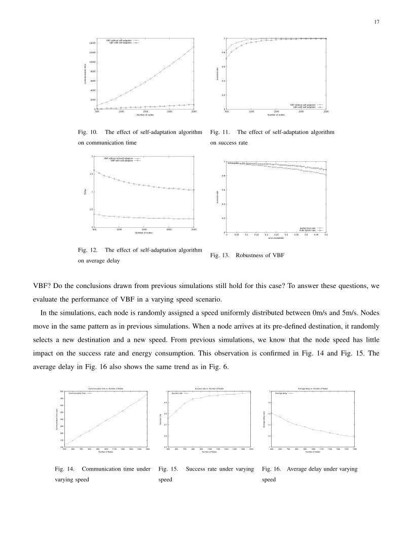
In the simulations, each node is randomly assigned a speed uniformly distributed between 0m/s and 5m/s. Nodes

move in the same pattern as in previous simulations. When a node arrives at its pre-defined destination, it randomly

selects a new destination and a new speed. From previous simulations, we know that the node speed has little

impact on the success rate and energy consumption. This observation is confirmed in Fig. 14 and Fig. 15. The

average delay in Fig. 16 also shows the same trend as in Fig. 6.

100

150

200

250

300

350

400

450

500

500 600 700 800 900 1000 1100 1200 1300 1400 1500

Com

mun

icat

ion

time

(sec

)

Number of Nodes

Communication time vs. Number of Nodes

Communication time

Fig. 14. Communication time under

varying speed

0.5

0.6

0.7

0.8

0.9

1

500 600 700 800 900 1000 1100 1200 1300 1400 1500

Suc

cess

rate

Number of Nodes

Success rate vs. Number of Nodes

Success rate

Fig. 15. Success rate under varying

speed

1

1.2

1.4

1.6

1.8

2

500 600 700 800 900 1000 1100 1200 1300 1400 1500

Ave

rage

del

ay (s

ec)

Number of Nodes

Average delay vs. Number of Nodes

Average delay

Fig. 16. Average delay under varying

speed

18

0

0.02

0.04

0.06

0.08

0.1

0 0.2 0.4 0.6 0.8 1 1.2 1.4 1.6 1.8 2 2.2 2.4 2.6 2.8 3 3.2 3.4 3.6 3.8 4 4.2 4.4 4.6 4.8 5

Com

mun

icat

ion

Tim

e P

er P

acke

t (S

econ

d)

Data Interval (Second)

Communication Time Per Pacaket vs Data Rate

communication time per packet

Fig. 17. Communication time vs

source data rate

0

0.2

0.4

0.6

0.8

1

0 0.2 0.4 0.6 0.8 1 1.2 1.4 1.6 1.8 2 2.2 2.4 2.6 2.8 3 3.2 3.4 3.6 3.8 4 4.2 4.4 4.6 4.8 5

Suc

cess

Rat

e (%

)

Data Interval (Second)

Communication Time Per Pacaket vs Data Rate

success rate

Fig. 18. Success rate vs source data

rate

0

0.5

1

1.5

2

0 0.2 0.4 0.6 0.8 1 1.2 1.4 1.6 1.8 2 2.2 2.4 2.6 2.8 3 3.2 3.4 3.6 3.8 4 4.2 4.4 4.6 4.8 5

Ave

rage

Del

ay (

Sec

ond)

Data Interval (Second)

Communication Time Per Pacaket vs Data Rate

average delay

Fig. 19. Average delay vs source data

rate

H. Impact of Source Data Rate

In previous simulations, we fix the source data rate as 2 packets per second in order to minimize the packet

transmission interference. A natural question is: will the source data rate affect the performance of VBF? Is 2

packets per second a good choice for the simulations? To answer these questions, we evaluate the impact of source

data rate on the performance of VBF.

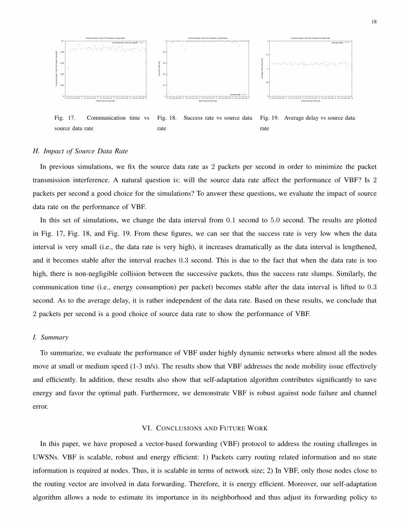
In this set of simulations, we change the data interval from 0.1 second to 5.0 second. The results are plotted

in Fig. 17, Fig. 18, and Fig. 19. From these figures, we can see that the success rate is very low when the data

interval is very small (i.e., the data rate is very high), it increases dramatically as the data interval is lengthened,

and it becomes stable after the interval reaches 0.3 second. This is due to the fact that when the data rate is too

high, there is non-negligible collision between the successive packets, thus the success rate slumps. Similarly, the

communication time (i.e., energy consumption) per packet) becomes stable after the data interval is lifted to 0.3

second. As to the average delay, it is rather independent of the data rate. Based on these results, we conclude that

2 packets per second is a good choice of source data rate to show the performance of VBF.

I. Summary

To summarize, we evaluate the performance of VBF under highly dynamic networks where almost all the nodes

move at small or medium speed (1-3 m/s). The results show that VBF addresses the node mobility issue effectively

and efficiently. In addition, these results also show that self-adaptation algorithm contributes significantly to save

energy and favor the optimal path. Furthermore, we demonstrate VBF is robust against node failure and channel

error.

VI. CONCLUSIONS AND FUTURE WORK

In this paper, we have proposed a vector-based forwarding (VBF) protocol to address the routing challenges in

UWSNs. VBF is scalable, robust and energy efficient: 1) Packets carry routing related information and no state

information is required at nodes. Thus, it is scalable in terms of network size; 2) In VBF, only those nodes close to

the routing vector are involved in data forwarding. Therefore, it is energy efficient. Moreover, our self-adaptation

algorithm allows a node to estimate its importance in its neighborhood and thus adjust its forwarding policy to

19

save more energy; 3) VBF utilizes path redundancy (controlled by the routing pipe radius) to provide robustness

against packet loss and node failure. Our simulation results have demonstrated the promising performance of VBF.

Future Work There are several directions in UWSNs worth future investigation. 1) In the VBF simulations, we

use a simple MAC protocol as the underlying link layer protocol. This is not a satisfactory choice. Designing an

efficient MAC protocol for underwater sensor networks is desirable for the next step. 2) We also plan to study the

reliable data transfer and congestion control problems, which are very challenging due to the unique features of

UWSNs: high end-to-end delay, low bandwidth, and high error probability.

REFERENCES

[1] C. Adjih, T. Clausen, P. Jacquet, A. Laouiti, P. Minet, P. Muhlethaler, A. Qayyum, and L. Viennot. Optimized Link State Routing

Protocol, March 2003.

[2] I. F. Akyildiz, D. Pompili, and T. Melodia. Challenges for Efficient Communication in Underwater Acoustic Sensor Networks. ACM

SIGBED Review, Vol. 1(1), July 2004.

[3] S. Basagni, I. Chlamtac, V. R. Syrotiuk, and B. A. Woodward. A Distance Routing Effect Algorithm for Mobility (DREAM). In

MOBICOM’98, pages 76–84, Dallas, Texas, USA, Oct. 1998.

[4] D. Braginsky and D. Estrin. Rumor Routing Algorithm For Sensor Networks. In WSNA’02, Atlanta, Georgia, USA, September 2002.

[5] J.-H. Cui, J. Kong, M. Gerla, and S. Zhou. Challenges: Building Scalable and Distributed Underwater Wireless Sensor Networks

(UWSNs) for Aquatic Applications . Technical report, UCONN CSE Technical Report: UbiNet-TR05-02 (BECAT/CSE-TR-05-5), Jan.

2005.

[6] H. Fuβler, J. Widmer, M. Kasemann, M. Mauve, and H. Hartenstein. Contention-Based Forwarding for Mobile Ad-Hoc Networks.

Elsevier’s Ad-Hoc Networks, Nov. 2003.

[7] M. Grossglauser and M. Vetterli. Locating Nodes with Ease: Mobility Diffusion of Last Encounters in Ad Hoc Networks. In IEEE

INFOCOM’03, Francisco,USA, Mar. 2003.

[8] J. Heidemann, Y. Li, A. Syed, J. Wills, and W. Ye. Underwater sensor networking: Research challenges and potential applications.

USC/ISI Technical Report ISI-TR-2005-603, 2005.

[9] W. R. Heinzelman, J. Kulik, and H. Balakrishnan. Adaptive Protocols for Information Dissemination in Wireless Sensor Networks. In

Mobicom’99, Seattle, Washington, USA, August 1999.

[10] M. Heissenbuttel, T. Braun, T. Bernoulli, and M. Walchi. BLR:Beacon-Less Routing Algorithm for Mobile Ad-Hoc Networks. Elsevier’s

Computer Communication Journal(Special Issue), 2003.

[11] C. Intanagonwiwat, R. Govindan, and D. Estrin. Directed Diffusion: A Scalable and Roust Communication Paradigm for Sensor

Networks. In ACM International Conference on Mobile Computing and Networking (MOBICOM’00), Boston, Massachusetts, USA,

August 2000.

[12] D. B. Johnson and D. A. Maltz. Dynamic Source Routing in Ad Hoc Wireless Networks. 353:153–181, 1996.

[13] B. Karp and H. Kung. GPSR: Greedy Perimeter Stateless Routing for Wirelss Networks. In MOBICOM’00, Boston, MA, USA, August

2000.

[14] D. B. Kilfoyle and A. B. Baggeroer. The State of the Art in Underwater Acoustic Telemetry. IEEE Journal of Oceanic Engineering,

OE-25(5):4–27, January 2000.

[15] J. Kong, J.-H. Cui, D. Wu, and M. Gerla. Building Underwater Ad-hoc Networks and Sensor Networks for Large Scale Real-time

Aquatic Applications . In IEEE Military Communications Conference (MILCOM’05), 2005.

[16] S. Lee, B. Bhattacharjee, and S. Banerjee. Efficient Geographic Routing in Multihop Wireless Networks. In ACM Mobihoc’05, May

2005.

20

[17] D. Niculescu and B. Nath. Trajectory Based Forwarding and Its Application. In ACM International Conference on Mobile Computing

and Networking (MOBICOM’03), San Diego, California, USA, September 2003.

[18] R. Ogier, M. Lewis, and F. Templin. Topology Dissemination Based on Reverse-Path Forwarding (TBRPF), March 2003.

[19] C. E. Perkins and P. Bhagwat. Highly Dynamic Destination-Sequenced Distance-Vector Routing (DSDV) for Mobile Computers. In

ACM SIGCOMM, pages 234–244, 1994.

[20] C. E. Perkins and E. M. Royer. Ad-Hoc On-Demand Distance Vector Routing. In IEEE WMCSA’99, pages 90–100, 1999.

[21] J. Proakis, E.M.Sozer, J. A. Rice, and M.Stojanovic. Shallow Water Acoustic Networks. IEEE Communications Magazines, pages

114–119, November 2001.

[22] J. G. Proakis, J. A. Rice, E. M. Sozer, and M. Stojanovic. Shallow Water Acoustic Networks. Ed. John Wiley and sons, 2001.

[23] K. Seada, M. Zuniga, A. Helmy, and B. Krishnamachari. Energy-Efficient Forwarding Strategies for Geographic Routing in Lossy

Wireless Sensor Networks. In ACM SenSys’04, Baltimore, Maryland, USA, November 2004.

[24] G. G. Xie and J. Gibson. A Networking Protocol for Underwater Acoustic Networks. In Technical Report TR-CS-00-02, Department

of Computer Science, Naval Postgraduate School, December 2000.

[25] F. Ye, H. Luo, J. Cheng, S. Lu, and L. Zhang. A Two-tier Data Dissemination Model for Large-scale Wireless Sensor Networks. In

MOBICOM’02, Atlanta, Georgia, USA, September 2002.

[26] F. Ye, G. Zhong, S. lu, and L. Zhang. GRAdient Broadcast: A Robust Data Delivery Protocol for Large Scale Sensor Networks. ACM

Wireless Networks(WINET), Vol.11(2), March 2005. The earlier version appears in IPSN2003.

[27] M. Zorzi and R. R. Rao. Geographic Random Forwarding(GeRaF) For ad hoc and sensor networks:multihop performance. IEEE Trans.

on Mobile Computing, Vol.2(4), Oct-Dec 2003.