vật lý 2,dhspkthcm

103 © 2014 Cengage Learning. All Rights Reserved. May not be scanned, copied or duplicated, or posted to a publicly accessible website, in whole or in part.

25 Electric Potential

CHAPTER OUTLINE

25.1 Electric Potential and Potential Difference

25.2 Potential Difference in a Uniform Electric Field

25.3 Electric Potential and Potential Energy Due to Point Charges

25.4 Obtaining the Value of the Electric Field

from the Electric Potential

25.5 Electric Potential Due to Continuous Charge Distributions

25.6 Electric Potential Due to a Charged Conductor

25.7 The Millikan Oil-Drop Experiment

25.8 Applications of Electrostatics

* An asterisk indicates a question or problem new to this edition.

ANSWERS TO OBJECTIVE QUESTIONS

OQ25.1 Answer (b). Taken without reference to any other point, the potential could have any value.

OQ25.2 Answer (d). The potential is decreasing toward the bottom of the page, so the electric field is downward.

OQ25.3 (i) Answer (c). The two spheres come to the same potential, so Q/R is the same for both. If charge q moves from A to B, we find the charge on B:

QA

RA

=QB

RB

→450 nC − q

1.00 cm=

q2.00 cm

→ q =900 nC

3= 300 nC

Sphere A has charge 450 nC – 300 nC = 150 nC.

(ii) Answer (a). Contact between conductors allows all charge to flow to the exterior surface of sphere B.

CuuDuongThanCong.com https://fb.com/tailieudientucntt

cuu d

uong

than

cong

. com

http://cuuduongthancong.com?src=pdf

https://fb.com/tailieudientucntt


© 2014 Cengage Learning. All Rights Reserved. May not be scanned, copied or duplicated, or posted to a publicly accessible website, in whole or in part.

OQ25.4 Answer (d).

Ex = − ΔV

Δx= −

1.90× 102 V − 1.20× 102 V( )5.00 m − 3.00 m( ) = −35.0 N/C

OQ25.5 Ranking a > b = d > c. The potential energy of a system of two charges is U = keq1q2 r . The potential energies are: (a) U = 2keQ

2 r , (b) U = keQ

2 r , (c) U = −keQ2 2r , (d) U = keQ

2 r .

OQ25.6 (i) Answer (a). The particle feels an electric force in the negative x direction. An outside agent pushes it uphill against this force, increasing the potential energy.

(ii) Answer (c). The potential decreases in the direction of the electric field.

OQ25.7 Ranking D > C > B > A. Let L be length of a side of the square. The potentials are:

VA =

keQL

+2keQ

2L= 1+ 2( ) keQ

L

VB =

2keQL

+keQ

2L= 2 +

12

⎛⎝⎜

⎞⎠⎟

keQL

VC =

keQ2L 2

+2keQ2L 2

= 3 2keQL

VD =

keQL 2

+2keQL 2

= 6keQL

OQ25.8 Answer (a). The change in kinetic energy is the negative of the change in electric potential energy:

ΔK = −qΔV = − −e( )V = e 1.00× 104 V( )= 1.00× 104 eV

OQ25.9 Ranking c > a > d > b. We add the electric potential energies of all possible pairs. They are:

(a) 3

keQ2

d

(b) −2

keQ2

d+

keQ2

d= −

keQ2

d

(c) 4

keQ2

d+ 2

keQ2

2d= 4 + 2( ) keQ

2

d

(d) 2

keQ2

d+

keQ2

2d− 2

keQ2

d−

keQ2

2d= 0


cuu d

uong

than

cong

. com



Chapter 25 105


OQ25.10 Answer (b). All charges are the same distance from the center. The potentials from the +1.50-µC, –1.00-µC, and –0.500-µC charges cancel.

OQ25.11 Answer (b). The work done on the proton equals the negative of the change in electric potential energy:

W = −qΔV → qΔV = −W = −qEscosθ

=− e 8.50 × 102 N/C( ) 2.50 m( ) 1( ) = −3.40 × 10−16 J

OQ25.12 (i) Answer (b). At points off the x axis the electric field has a nonzero y component. At points on the negative x axis the field is to the right and positive. At points to the right of x = 0.500 m the field is to the left and nonzero. The field is zero at one point between x = 0.250 m and x = 0.500 m.

(ii) Answer (c). The electric potential is negative at this and at all points because both charges are negative.

(iii) Answer (d). The potential cannot be zero at a finite distance because both charges are negative.

OQ25.13 Answer (b). The same charges at the same distance away create the same contribution to the total potential.

OQ25.14 The ranking is e > d > a = c > b. The change in kinetic energy is the negative of the change in electric potential energy, so we work out

−qΔV = −q Vf −Vi( ) in each case.

(a) –(–e)(60 V – 40 V) = +20 eV (b) –(–e)(20 V – 40 V) = –20 eV

(c) –(e)(20 V – 40 V) = +20 eV (d) –(e)(10 V – 40 V) = +30 eV

(e) –(–2e)(60 V – 40 V) = +40 eV

OQ25.15 Answer (b). The change in kinetic energy is the negative of the change in electric potential energy:

ΔK = −qΔV → KB − KA = q VA −VB( )

12

mvB2 = 1

2mvA

2 + 2e( ) VA −VB( )

Solving for the speed gives

vB = vA2 +

4e VA −VB( )m

= 6.20× 105 m/s( )2+

4 1.60× 10−19 C( ) 1.50× 103 V − 4.00× 103 V( )6.63× 10−27 kg

= 3.78× 105 m/s


cuu d

uong

than

cong

. com





ANSWERS TO CONCEPTUAL QUESTIONS

CQ25.1 The main factor is the radius of the dome. One often overlooked aspect is also the humidity of the air—drier air has a larger dielectric breakdown strength, resulting in a higher attainable -electric potential. If other grounded objects are nearby, the maximum potential might be reduced.

CQ25.2 (a) The proton accelerates in the direction of the electric field, (b) its kinetic energy increases as (c) the electric potential energy of the system decreases.

CQ25.3 To move like charges together from an infinite separation, at which the potential energy of the system of two charges is zero, requires work to be done on the system by an outside agent. Hence energy is stored, and potential energy is positive. As charges with opposite signs move together from an infinite separation, energy is released, and the potential energy of the set of charges becomes negative.

CQ25.4 (a) The grounding wire can be touched equally well to any point on the sphere. Electrons will drain away into the ground.

(b) The sphere will be left positively charged. The ground, wire, and sphere are all conducting. They together form an equipotential volume at zero volts during the contact. However close the grounding wire is to the negative charge, electrons have no difficulty in moving within the metal through the grounding wire to ground. The ground can act as an infinite source or sink of electrons. In this case, it is an electron sink.

CQ25.5 When one object B with electric charge is immersed in the electric field of another charge or charges A, the system possesses electric potential energy. The energy can be measured by seeing how much work the field does on the charge B as it moves to a reference location. We choose not to visualize A’s effect on B as an action-at-a-distance, but as the result of a two-step process: Charge A creates electric potential throughout the surrounding space. Then the potential acts on B to inject the system with energy.

CQ25.6 (a) The electric field is cylindrically radial. The equipotential surfaces are nesting coaxial cylinders around an infinite line of charge.

(b) The electric field is spherically radial. The equipotential surfaces are nesting concentric spheres around a uniformly charged sphere.


cuu d

uong

than

cong

. com



Chapter 25 107


SOLUTIONS TO END-OF-CHAPTER PROBLEMS

Section 25.1 Electric Potential and Potential Difference

Section 25.2 Potential Difference in a Uniform Electric Field *P25.1 (a) From Equation 25.6,

E = ΔV

d= 600 J/C

5.33× 10−3 m= 1.13× 105 N/C

(b) The force on an electron is given by

F = q E = 1.60× 10−19 C( ) 1.13× 105 N/C( ) = 1.80× 10−14 N

(c) Because the electron is repelled by the negative plate, the force used to move the electron must be applied in the direction of the electron's displacement. The work done to move the electron is

W = F ⋅ scosθ = 1.80× 10−14 N( ) 5.33− 2.00( )× 10−3 m⎡⎣ ⎤⎦cos0°

= 4.37 × 10−17 J

*P25.2 (a) We follow the path from (0, 0) to (20.0 cm, 0) to (20.0 cm, 50.0 cm).

ΔU = − (work done)

ΔU = − [work from origin to (20.0 cm, 0)]

– [work from (20.0 cm, 0) to (20.0 cm, 50.0 cm)]

Note that the last term is equal to 0 because the force is perpendicular to the displacement.

ΔU = − qEx( )Δx = − 12.0 × 10−6 C( ) 250 V m( ) 0.200 m( )

= −6.00 × 10−4 J

(b) ΔV = ΔU

q= − 6.00 × 10−4 J

12.0 × 10−6 C= −50.0 J C = −50.0 V

P25.3 (a) Energy of the proton-field system is conserved as the proton moves from high to low potential, which can be defined for this problem as moving from 120 V down to 0 V.

Ki +Ui = K f +U f : 0 + qV =

12

mvp2 + 0

1.60 × 10−19 C( ) 120 V( ) 1 J1 V ⋅C

⎛⎝⎜

⎞⎠⎟ =

12

1.67 × 10−27 kg( )vp2

vp = 1.52 × 105 m/s


cuu d

uong

than

cong

. com





(b) The electron will gain speed in moving the other way,

from Vi = 0 to Vf = 120 V: Ki + Ui = Kf + Uf

0 + 0 =12

mve2 + qV

0 =12

9.11× 10−31 kg( )ve2 + −1.60 × 10−19 C( ) 120 J/C( )

ve = 6.49 × 106 m/s

P25.4 The potential difference is

ΔV = Vf −Vi = −5.00 V − 9.00 V = −14.0 V

and the total charge to be moved is

Q = −NAe = − 6.02 × 1023( ) 1.60 × 10−19 C( ) = −9.63 × 104 C

Now, from ΔV =

WQ

, we obtain

W = QΔV = (−9.63× 104 C)(−14.0 J/C) = 1.35 MJ

P25.5 The electric field is uniform. By Equation 25.3,

VB −VA = −E ⋅ds

A

B

∫ = −E ⋅ds

A

C

∫ −E ⋅ds

C

B

∫

VB −VA = −Ecos180°( ) dy−0.300

0.500

∫ − Ecos90.0°( ) dx−0.200

0.400

∫VB −VA = 325 V/m( ) 0.800 m( ) = +260 V

P25.6 Assume the opposite. Then at some point A on some equipotential surface the electric field has a nonzero component Ep in the plane of the surface. Let a test charge start from point A and move some distance on the surface in the direction of the field component. Then

ΔV = −

E ⋅ds

A

B

∫ is nonzero. The electric potential charges across the

surface and it is not an equipotential surface. The contradiction shows that our assumption is false, that Ep = 0, and that the field is perpendicular to the equipotential surface.


cuu d

uong

than

cong

. com



Chapter 25 109


P25.7 We use the energy version of the isolated system model to equate the energy of the electron-field system when the electron is at x = 0 to the energy when the electron is at x = 2.00 cm. The unknown will be the difference in potential Vf – Vi . Thus, Ki + Ui = Kf + Uf becomes

12

mvi2 + qVi =

12

mv f2 + qVf

or

12

m vi2 − v f

2( ) = q Vf −Vi( ) ,

so Vf −Vi = ΔV =

m vi2 − v f

2( )2q

.

(a) Noting that the electron’s charge is negative, and evaluating the potential difference, we have

ΔV =9.11× 10–31 kg( ) (3.70 × 106 m/s)2 – (1.40 × 105 m/s)2⎡⎣ ⎤⎦

2 –1.60 × 10–19 C( )= −38.9 V

(b) The negative sign means that the 2.00-cm location is lower in potential than the origin:

The origin is at the higher potential.

P25.8 (a) The electron-electric field is an isolated system:

Ki +Ui = K f +U f

12

mevi2 + −e( )Vi = 0+ −e( )Vf

e Vf −Vi( ) = − 12

mevi2

The potential difference is then

ΔVe = − mevi2

2e= −

9.11× 10−31 kg( ) 2.85× 107 m/s( )2

2 1.60× 10−19 C( )= −2.31× 103 V = −2.31 kV

(b) From (a), we see that the stopping potential is proportional to the kinetic energy of the particle.

Because a proton is more massive than an electron, a protontraveling at the same speed as an electron has more initial kineticenergy and requires a greater magnitude stopping potential.


cuu d

uong

than

cong

. com





(c) The proton-electric field is an isolated system:

Ki +Ui = K f +U f

12

mpvi2 + eVi = 0+ eVf

e Vf −Vi( ) = 12

mpvi2

The potential difference is

ΔVp =

mpvi2

2e

Therefore, from (a),

ΔVp

ΔVe

=mpvi

2 2e

−mevi2 2e

→ ΔVp ΔVe = −mp me

P25.9 Arbitrarily take V = 0 at point P. Then the potential at the original position of the charge is (by Equation 25.3)

ΔV = V − 0 = V = −E ⋅ s = −ELcosθ (relative to P)

At the final point a,

V = –EL (relative to P)

Because the table is frictionless and the particle-field system is isolated, we have

K +U( )i = K +U( ) f

or 0− qELcosθ = 1

2mv2 − qEL

solving for the speed gives

v = 2qEL 1− cosθ( )m

=2 2.00× 10−6 C( ) 300 N/C( ) 1.50 m( ) 1− cos60.0°( )

0.010 0 kg

= 0.300 m/s

P25.10 (a) The system consisting of the mass-spring-electric field is

isolated.

(b) The system has both electric potential energy and elastic potential energy: Ue and Usp.


cuu d

uong

than

cong

. com



Chapter 25 111


(c) Taking the electric potential to be zero at the initial configuration, after the block has stretched the spring a distance x, the final electric potential is (from equation 25.3)

ΔV = V = −E ⋅ s = −Ex

By energy conservation within the system,

K +Usp +Ue( )i= K +Usp +Ue( )

f

0 + 0 + 0 = 0 +12

kx2 +QV

0 =12

kx2 +Q −Ex( ) → x =2QE

k

(d) Particle in equilibrium

(e)

F∑ = 0 → − kx0 +QE = 0 → x0 =QEk

(f) The particle is no longer in equilibrium; therefore, the force equation becomes

F∑ = ma → − kx +QE = md2xdt2

− k x − QEk

⎛⎝⎜

⎞⎠⎟ = m

d2xdt2

Defining ′x = x − x0 , we have

d2 ′xdt2 =

d2 x − x0( )dt2 =

d2xdt2

.

Substitute ′x = x − x0 into the force equation:

−k x −QEk

⎛⎝⎜

⎞⎠⎟ = m

d2xdt2 → − k ′x = m

d2 ′xdt2

→ d2 ′xdt2 = −

k ′xm

(g) The result of part (f) is the equation for simple harmonic motion

a ′x = −ω 2 ′x with

ω =

km

=2πT

→ T =2πω

= 2π mk

(h)

The period does not depend on the electric field. The electric fieldjust shifts the equilibrium point for the spring, just like a gravita-tional field does for an object hanging from a vertical spring.


cuu d

uong

than

cong

. com





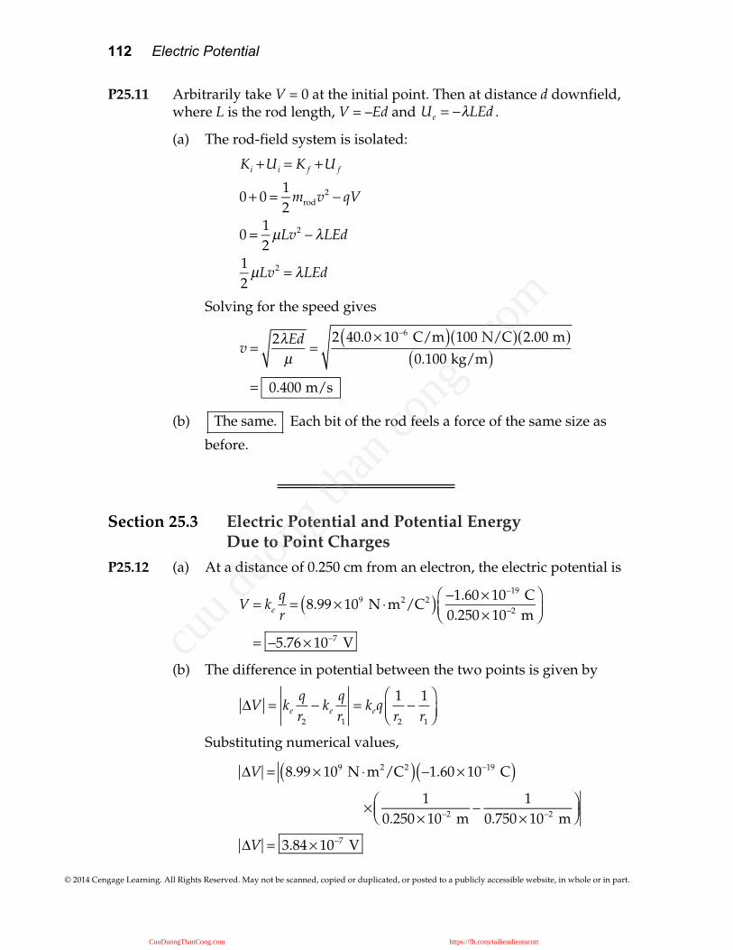
P25.11 Arbitrarily take V = 0 at the initial point. Then at distance d downfield, where L is the rod length, V = –Ed and Ue = −λLEd .

(a) The rod-field system is isolated:

Ki +Ui = K f +U f

0+ 0 = 12

mrodv2 − qV

0 = 12µLv2 − λLEd

12µLv2 = λLEd


v = 2λEdµ

=2 40.0× 10−6 C/m( ) 100 N/C( ) 2.00 m( )

0.100 kg/m( )= 0.400 m/s

(b)

The same. Each bit of the rod feels a force of the same size as

before.

Section 25.3 Electric Potential and Potential Energy Due to Point Charges

P25.12 (a) At a distance of 0.250 cm from an electron, the electric potential is

V = keqr= 8.99× 109 N ⋅m2/C2( ) −1.60× 10−19 C

0.250× 10−2 m⎛⎝⎜

⎞⎠⎟

= −5.76× 10−7 V

(b) The difference in potential between the two points is given by

ΔV = ke

qr2

− ke

qr1

= keq1r2

−1r1

⎛⎝⎜

⎞⎠⎟

Substituting numerical values,

ΔV = 8.99× 109 N ⋅m2/C2( ) −1.60× 10−19 C( ) × 1

0.250× 10−2 m− 1

0.750× 10−2 m⎛⎝⎜

⎞⎠⎟

ΔV = 3.84× 10−7 V


cuu d

uong

than

cong

. com



Chapter 25 113


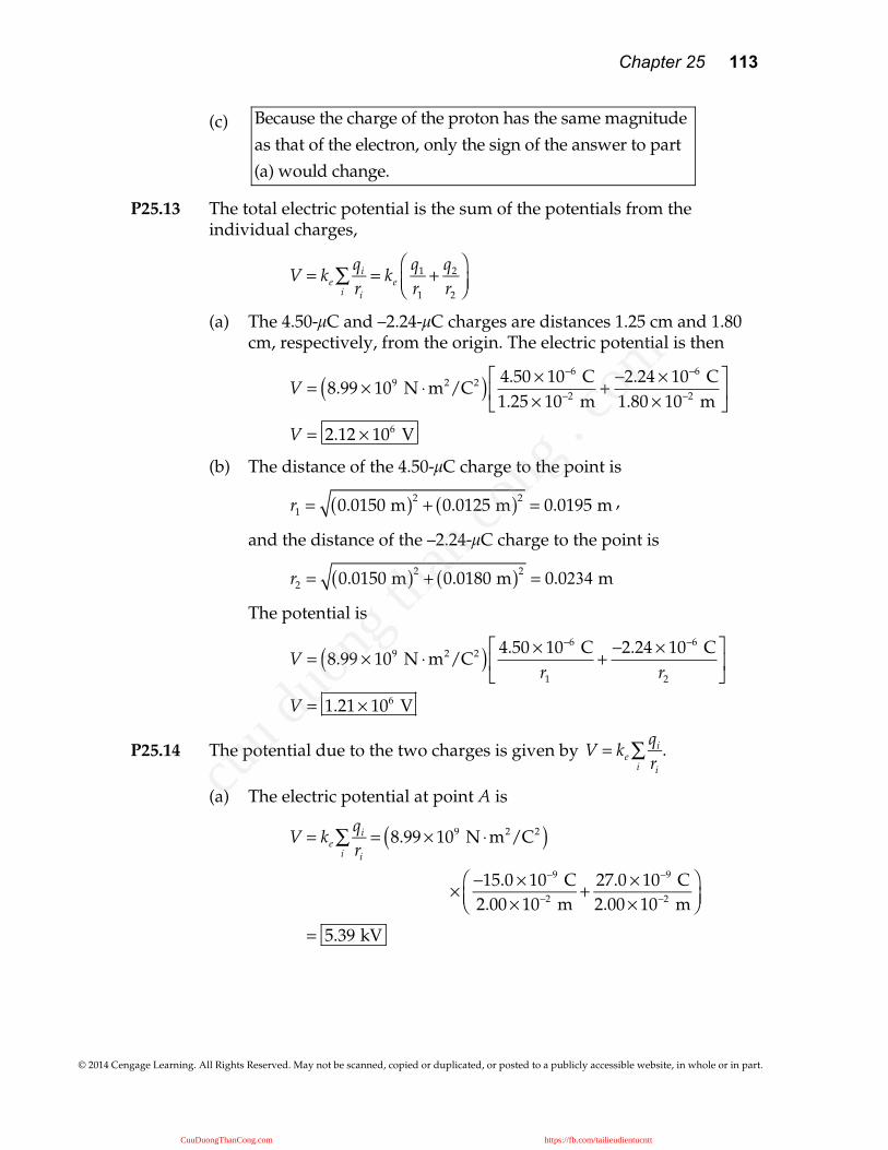
(c)

Because the charge of the proton has the same magnitude as that of the electron, only the sign of the answer to part (a) would change.

P25.13 The total electric potential is the sum of the potentials from the individual charges,

V = ke

qi

rii∑ = ke

q1

r1

+ q2

r2

⎛⎝⎜

⎞⎠⎟

(a) The 4.50-µC and –2.24-µC charges are distances 1.25 cm and 1.80 cm, respectively, from the origin. The electric potential is then

V = 8.99 × 109 N ⋅m2/C2( ) 4.50 × 10−6 C1.25 × 10−2 m

+−2.24 × 10−6 C1.80 × 10−2 m

⎡

⎣⎢

⎤

⎦⎥

V = 2.12 × 106 V

(b) The distance of the 4.50-µC charge to the point is

r1 = 0.0150 m( )2 + 0.0125 m( )2 = 0.0195 m ,

and the distance of the –2.24-µC charge to the point is

r2 = 0.0150 m( )2 + 0.0180 m( )2 = 0.0234 m

The potential is

V = 8.99 × 109 N ⋅m2/C2( ) 4.50 × 10−6 Cr1

+−2.24 × 10−6 C

r2

⎡

⎣⎢

⎤

⎦⎥

V = 1.21× 106 V

P25.14 The potential due to the two charges is given by V = ke

qi

rii∑ .

(a) The electric potential at point A is

V = keqi

rii∑ = 8.99× 109 N ⋅m2/C2( )

× −15.0 × 10−9 C2.00× 10−2 m

+ 27.0 × 10−9 C2.00× 10−2 m

⎛⎝⎜

⎞⎠⎟

= 5.39 kV


cuu d

uong

than

cong

. com





(b) The electric potential at point B is

V = keqi

rii∑ = 8.99× 109 N ⋅m2/C2( )

× −15.0 × 10−9 C1.00× 10−2 m

+ 27.0 × 10−9 C1.00× 10−2 m

⎛⎝⎜

⎞⎠⎟

= 10.8 kV

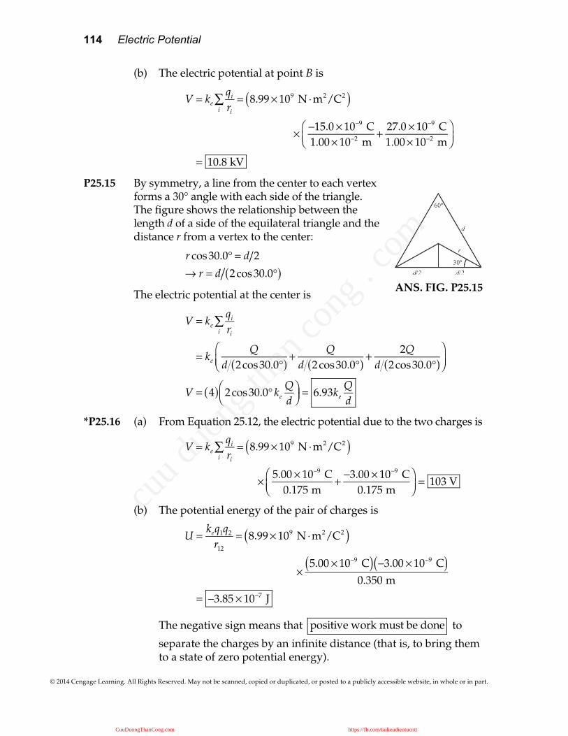
P25.15 By symmetry, a line from the center to each vertex forms a 30° angle with each side of the triangle. The figure shows the relationship between the length d of a side of the equilateral triangle and the distance r from a vertex to the center:

r cos30.0° = d 2→ r = d 2cos30.0°( )

The electric potential at the center is

V = keqi

rii∑

= keQ

d 2cos30.0°( ) +Q

d 2cos30.0°( ) +2Q

d 2cos30.0°( )⎛⎝⎜

⎞⎠⎟

V = 4( ) 2cos30.0° keQd

⎛⎝⎜

⎞⎠⎟ = 6.93ke

Qd

*P25.16 (a) From Equation 25.12, the electric potential due to the two charges is

V = keqi

rii∑ = 8.99× 109 N ⋅m2/C2( )

× 5.00 × 10−9 C0.175 m

+ −3.00 × 10−9 C0.175 m

⎛⎝⎜

⎞⎠⎟= 103 V

(b) The potential energy of the pair of charges is

U = keq1q2

r12

= 8.99× 109 N ⋅m2/C2( )

×5.00 × 10−9 C( ) −3.00 × 10−9 C( )

0.350 m

= −3.85 × 10−7 J

The negative sign means that

positive work must be done to

separate the charges by an infinite distance (that is, to bring them to a state of zero potential energy).

ANS. FIG. P25.15


cuu d

uong

than

cong

. com



Chapter 25 115


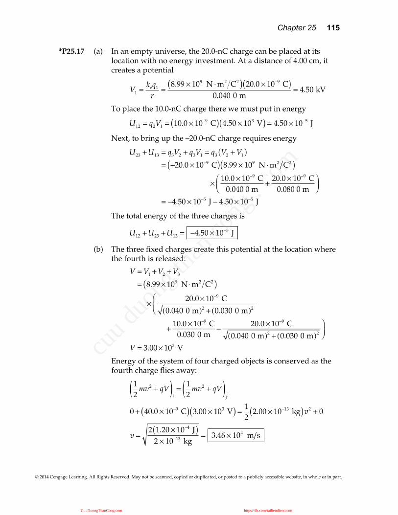
*P25.17 (a) In an empty universe, the 20.0-nC charge can be placed at its location with no energy investment. At a distance of 4.00 cm, it creates a potential

V1 =

keq1

r=

8.99 × 109 N ⋅m2 C2( ) 20.0 × 10−9 C( )0.040 0 m

= 4.50 kV

To place the 10.0-nC charge there we must put in energy

U12 = q2V1 = 10.0 × 10−9 C( ) 4.50 × 103 V( ) = 4.50 × 10−5 J

Next, to bring up the –20.0-nC charge requires energy

U23 +U13 = q3V2 + q3V1 = q3 V2 +V1( )= −20.0 × 10−9 C( ) 8.99 × 109 N ⋅m2 C2( ) × 10.0 × 10−9 C

0.040 0 m+ 20.0 × 10−9 C

0.080 0 m⎛⎝⎜

⎞⎠⎟

= −4.50 × 10−5 J − 4.50 × 10−5 J

The total energy of the three charges is

U12 +U23 +U13 = −4.50 × 10−5 J

(b) The three fixed charges create this potential at the location where the fourth is released:

V = V1 +V2 +V3

= 8.99× 109 N ⋅m2 C2( )

× 20.0× 10−9 C0.040 0 m( )2 + 0.030 0 m( )2

⎛⎝⎜

+ 10.0× 10−9 C0.030 0 m

− 20.0× 10−9 C0.040 0 m( )2 + 0.030 0 m( )2

⎞⎠⎟

V = 3.00× 103 V

Energy of the system of four charged objects is conserved as the fourth charge flies away:

12

mv2 + qV( )i= 1

2mv2 + qV( )

f

0 + 40.0 × 10−9 C( ) 3.00 × 103 V( ) = 12

2.00 × 10−13 kg( )v2 + 0

v =2 1.20 × 10−4 J( )

2 × 10−13 kg= 3.46 × 104 m s


cuu d

uong

than

cong

. com





P25.18 (a) VA = ke

qi

rii∑ = ke

Qd+ 2Q

d 2⎛⎝⎜

⎞⎠⎟ = ke

Qd

1+ 2( )

V = 8.99× 109 N ⋅m2/C2( ) 5.00 × 10−9 C

2.00× 10−2 m⎛⎝⎜

⎞⎠⎟

1+ 2( ) = 5.43 kV

(b) VB = ke

qi

rii∑ = ke

Qd 2

+ 2Qd

⎛⎝⎜

⎞⎠⎟ = ke

Qd

12+ 2⎛

⎝⎜⎞⎠⎟

VB = 8.99× 109 N ⋅m2/C2( ) 5.00 × 10−9 C

2.00× 10−2 m⎛⎝⎜

⎞⎠⎟

12+ 2⎛

⎝⎜⎞⎠⎟ = 6.08 kV

(c) VB −VA = ke

Qd

12+ 2⎛

⎝⎜⎞⎠⎟− ke

Qd

1+ 2( ) = keQd

12+ 1− 2⎛

⎝⎜⎞⎠⎟

VB −VA = 8.99× 109 N ⋅m2/C2( ) 5.00 × 10−9 C2.00× 10−2 m

⎛⎝⎜

⎞⎠⎟

12+ 1− 2⎛

⎝⎜⎞⎠⎟

= 658 V

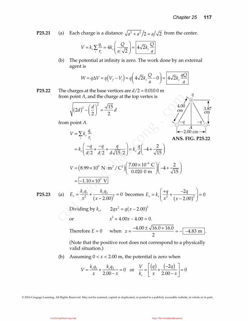
P25.19 (a) Since the charges are equal and placed symmetrically, F = 0 .

(b) Since F = qE = 0, E = 0 .

(c)

V = 2ke

qr

= 2 8.99 × 109 N ⋅m2 C2( ) 2.00 × 10−6 C0.800 m

⎛⎝⎜

⎞⎠⎟

V = 4.50 × 104 V = 45.0 kV

P25.20 At a distance r from a charged particle, the voltage is V =

keQr

and the

field magnitude is E =

ke Qr2 .

(a) r =

VE

=3.00 × 103 V

5.00 × 102 V m= 6.00 m

(b) V = −3 000 V =

Q4π ∈0 6.00 m( )

Then,

Q = 6.00 m( ) −3 000 V( ) 4π ∈0( ) = −2.00 µC

ANS. FIG. P25.19


cuu d

uong

than

cong

. com



Chapter 25 117


P25.21 (a) Each charge is a distance a2 + a2 2 = a 2 from the center.

V = ke

qi

rii∑ = 4ke

Qa 2

⎛⎝⎜

⎞⎠⎟= 4 2ke

Qa

(b) The potential at infinity is zero. The work done by an external agent is

W = qΔV = q Vf −Vi( ) = q 4 2ke

Qa− 0⎛

⎝⎜⎞⎠⎟ = 4 2ke

qQa

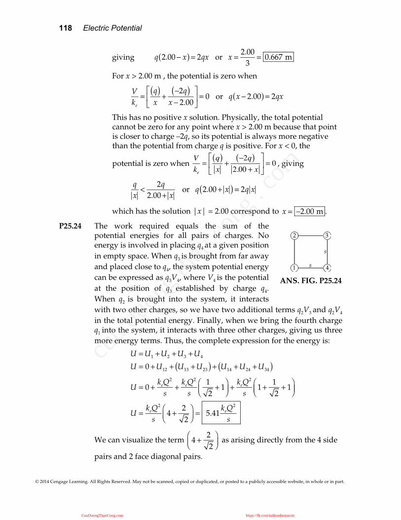
P25.22 The charges at the base vertices are d/2 = 0.010 0 m from point A, and the charge at the top vertex is

2d( )2 −d2

⎛⎝⎜

⎞⎠⎟

2

=152

d

from point A.

V = keqi

rii∑

= ke−qd 2

+ −qd 2

+ qd 15 2

⎛⎝⎜

⎞⎠⎟= ke

qd

−4+ 215

⎛⎝⎜

⎞⎠⎟

V = 8.99× 109 N ⋅m2 /C2( ) 7.00× 10−6 C0.020 0 m

⎛⎝⎜

⎞⎠⎟

−4+ 215

⎛⎝⎜

⎞⎠⎟

= −1.10× 107 V

P25.23 (a) Ex =

keq1

x2 +keq2

x − 2.00( )2 = 0 becomes Ex = ke

+qx2 +

−2qx − 2.00( )2

⎛

⎝⎜⎞

⎠⎟= 0

Dividing by ke, 2qx2 = q x − 2.00( )2

or x2 + 4.00x – 4.00 = 0.

Therefore E = 0 when x =

−4.00 ± 16.0 + 16.02

= − −4.83 m .

(Note that the positive root does not correspond to a physically valid situation.)

(b) Assuming 0 < x < 2.00 m, the potential is zero when

V = keq1

x+ keq2

2.00− x= 0 or

Vke

=q( )x

+−2q( )

2.00− x⎡

⎣⎢

⎤

⎦⎥ = 0

ANS. FIG. P25.22


cuu d

uong

than

cong

. com





giving q 2.00− x( ) = 2qx or x = 2.00

3= 0.667 m

For x > 2.00 m , the potential is zero when

Vke

=q( )x

+−2q( )

x − 2.00⎡

⎣⎢

⎤

⎦⎥ = 0 or q x − 2.00( ) = 2qx

This has no positive x solution. Physically, the total potential cannot be zero for any point where x > 2.00 m because that point is closer to charge –2q, so its potential is always more negative than the potential from charge q is positive. For x < 0, the

potential is zero when Vke

=q( )x

+−2q( )

2.00 + x⎡

⎣⎢

⎤

⎦⎥ = 0 , giving

qx< 2q

2.00+ x or q 2.00+ x( ) = 2q x

which has the solution |x| = 2.00 correspond to x = −2.00 m .

P25.24 The work required equals the sum of the potential energies for all pairs of charges. No energy is involved in placing q4 at a given position in empty space. When q3 is brought from far away and placed close to q4, the system potential energy can be expressed as q3V4, where V4 is the potential at the position of q3 established by charge q4. When q2 is brought into the system, it interacts with two other charges, so we have two additional terms q2V3 and q2V4

in the total potential energy. Finally, when we bring the fourth charge q1 into the system, it interacts with three other charges, giving us three more energy terms. Thus, the complete expression for the energy is:

U =U1 +U2 +U3 +U4

U = 0 +U12 + U13 +U23( ) + U14 +U24 +U34( )

U = 0 +keQ

2

s+

keQ2

s12+ 1⎛

⎝⎜⎞⎠⎟+

keQ2

s1+

12+ 1⎛

⎝⎜⎞⎠⎟

U =keQ

2

s4 +

22

⎛⎝⎜

⎞⎠⎟= 5.41

keQ2

s

We can visualize the term

4 +22

⎛⎝⎜

⎞⎠⎟

as arising directly from the 4 side

pairs and 2 face diagonal pairs.

ANS. FIG. P25.24


cuu d

uong

than

cong

. com



Chapter 25 119


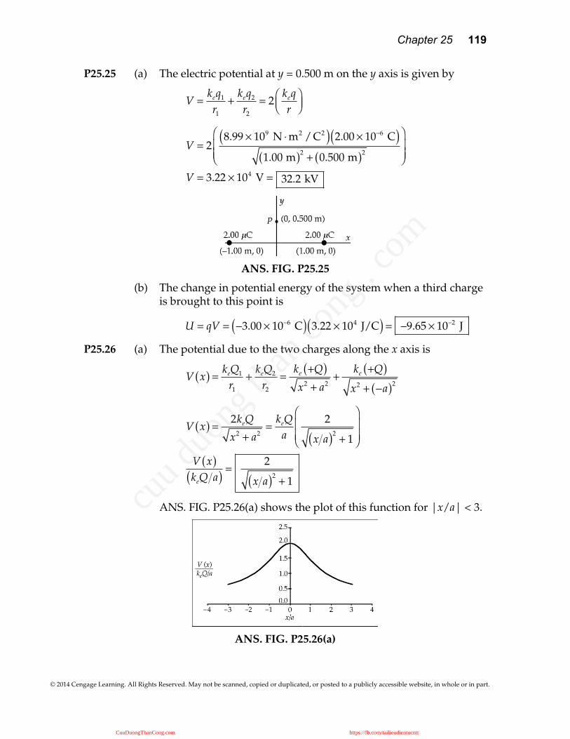
P25.25 (a) The electric potential at y = 0.500 m on the y axis is given by

V =

keq1

r1

+keq2

r2

= 2keqr

⎛⎝⎜

⎞⎠⎟

V = 28.99 × 109 N ⋅m2 / C2( ) 2.00 × 10−6 C( )

1.00 m( )2 + 0.500 m( )2

⎛

⎝⎜⎜

⎞

⎠⎟⎟

V = 3.22 × 104 V = 32.2 kV

ANS. FIG. P25.25

(b) The change in potential energy of the system when a third charge is brought to this point is

U = qV = −3.00 × 10−6 C( ) 3.22 × 104 J/C( ) = −9.65 × 10−2 J

P25.26 (a) The potential due to the two charges along the x axis is

V x( ) = keQ1

r1

+keQ2

r2

=ke +Q( )x2 + a2

+ke +Q( )

x2 + −a( )2

V x( ) = 2keQ

x2 + a2=

keQa

2

x a( )2 + 1

⎛

⎝⎜⎜

⎞

⎠⎟⎟

V x( )keQ a( ) =

2

x a( )2 + 1

ANS. FIG. P25.26(a) shows the plot of this function for |x/a| < 3.

ANS. FIG. P25.26(a)


cuu d

uong

than

cong

. com





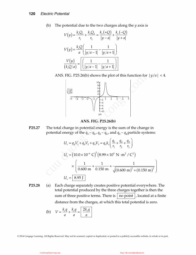
(b) The potential due to the two charges along the y axis is

V y( ) = keQ1

r1

+keQ2

r2

=ke +Q( )y − a

+ke −Q( )y + a

V y( ) = keQa

1y a − 1

−1

y a + 1

⎛

⎝⎜⎞

⎠⎟

V y( )keQ a( ) =

1y a − 1

−1

y a + 1

⎛

⎝⎜⎞

⎠⎟

ANS. FIG. P25.26(b) shows the plot of this function for |y/a| < 4.

ANS. FIG. P25.26(b)

P25.27 The total change in potential energy is the sum of the change in potential energy of the q1 – q4 , q2 – q4 , and q3 – q4 particle systems:

Ue = q4V1 + q4V2 + q4V3 = q4ke

q1

r1

+ q2

r2

+ q3

r3

⎛⎝⎜

⎞⎠⎟

Ue = 10.0 × 10−6 C( )28.99 × 109 N ⋅m2 / C2( )

×1

0.600 m+

10.150 m

+1

0.600 m( )2 + 0.150 m( )2

⎛

⎝⎜⎜

⎞

⎠⎟⎟

Ue = 8.95 J

P25.28 (a) Each charge separately creates positive potential everywhere. The total potential produced by the three charges together is then the sum of three positive terms. There is

no point , located at a finite

distance from the charges, at which this total potential is zero.

(b) V =

keqa

+keqa

=2keq

a


cuu d

uong

than

cong

. com



Chapter 25 121


P25.29 Each charge creates equal potential at the center. The total potential is

V = 5

ke −q( )R

⎡

⎣⎢

⎤

⎦⎥ = −

5keqR

P25.30 The original electrical potential energy is

Ue = qV = q

keqd

In the final configuration we have mechanical equilibrium. The spring and electrostatic forces on each charge are

Fspring + Fcharge = −k 2d( ) + q

keq3d( )2 = 0

Then k =

keq2

18d3

In the final configuration the total potential energy is

12

kx2 + qV =12

keq2

18d3 2d( )2 + qkeq3d

=49

keq2

d

The missing energy must have become internal energy, as the system is isolated:

ΔU + ΔEint = 0

4keq2

9d− keq

2

d+ ΔEint = 0

The increase in internal energy of the system is then

ΔEint =

5keq2

9d

P25.31 Consider the two spheres as a system. (a) Conservation of momentum:

0 = m1v1i + m2v2 − i( ) or

v2 =

m1v1

m2

By conservation of energy,

0 =

ke −q1( )q2

d=

12

m1v12 +

12

m2v22 +

ke −q1( )q2

r1 + r2

and

keq1q2

r1 + r2

−keq1q2

d=

12

m1v12 +

12

m12v1

2

m2

, which yields

v1 =

2m2keq1q2

m1 m1 + m2( )1

r1 + r2

−1d

⎛⎝⎜

⎞⎠⎟


cuu d

uong

than

cong

. com





suppressing units,

v1 =2 0.700( ) 8.99 × 109( ) 2 × 10−6( ) 3 × 10−6( )

0.100( ) 0.800( )1

8 × 10−3 −1

1.00⎛⎝⎜

⎞⎠⎟

= 10.8 m s

v2 =m1v1

m2

=0.100 kg( ) 10.8 m s( )

0.700 kg= 1.55 m s

(b) If the spheres are metal, electrons will move around on them with negligible energy loss to place the centers of excess charge on the insides of the spheres. Then just before they touch, the effective distance between charges will be less than r1 + r2 and the spheres

will really be moving

faster than calculated in (a) .

P25.32 Consider the two spheres as a system.

(a) Conservation of momentum:

0 = m1v1i + m2v2 − i( )

or v2 =

m1v1

m2

.

By conservation of energy,

0 =ke −q1( )q2

d=

12

m1v12 +

12

m2v22 +

ke −q1( )q2

r1 + r2

and

keq1q2

r1 + r2

−keq1q2

d=

12

m1v12 +

12

m12v1

2

m2

.

v1 =2m2keq1q2

m1 m1 + m2( )1

r1 + r2

−1d

⎛⎝⎜

⎞⎠⎟

v2 =m1

m2

⎛⎝⎜

⎞⎠⎟

v1 =2m1keq1q2

m2 m1 + m2( )1

r1 + r2

−1d

⎛⎝⎜

⎞⎠⎟

(b) If the spheres are metal, electrons will move around on them with negligible energy loss to place the centers of excess charge on the insides of the spheres. Then just before they touch, the effective distance between charges will be less than r1 + r2 and the spheres

will really be moving

faster than calculated in (a) .


cuu d

uong

than

cong

. com



Chapter 25 123


P25.33 A cube has 12 edges and 6 faces. Consequently, there are 12 edge pairs separated by s, 2 × 6 = 12 face diagonal pairs separated by 2s , and 4 interior diagonal pairs separated by 3s .

U =

keq2

s12 +

122+

43

⎡⎣⎢

⎤⎦⎥= 22.8

keq2

s

P25.34 Each charge moves off on its diagonal line. All charges have equal speeds.

K +U( )i∑ = K +U( ) f∑

0+ 4keq2

L+ 2keq

2

2L= 4

12

mv2⎛⎝⎜

⎞⎠⎟ +

4keq2

2L+ 2keq

2

2 2L

2 + 12

⎛⎝⎜

⎞⎠⎟

keq2

L= 2mv2


v = 1+ 1

8⎛⎝⎜

⎞⎠⎟

keq2

mL

P25.35 Using conservation of energy for the alpha particle-nucleus system,

we have K f +U f = Ki +Ui .

But Ui =

keqαqgold

ri

and ri ≈ ∞. Thus, Ui = 0.

Also, Kf = 0 (vf = 0 at turning point),

so Uf = Ki

or

keqαqgold

rmin

=12

mαvα2

rmin =2keqαqgold

mαvα2

=2 8.99 × 109 N ⋅m2 / C2( ) 2( ) 79( ) 1.60 × 10−19 C( )2

6.64 × 10−27 kg( ) 2.00 × 107 m/s( )2

= 2.74 × 10−14 m = 27.4 fm


cuu d

uong

than

cong

. com





Section 25.4 Obtaining the Value of the Electric Field from the Electric Potential

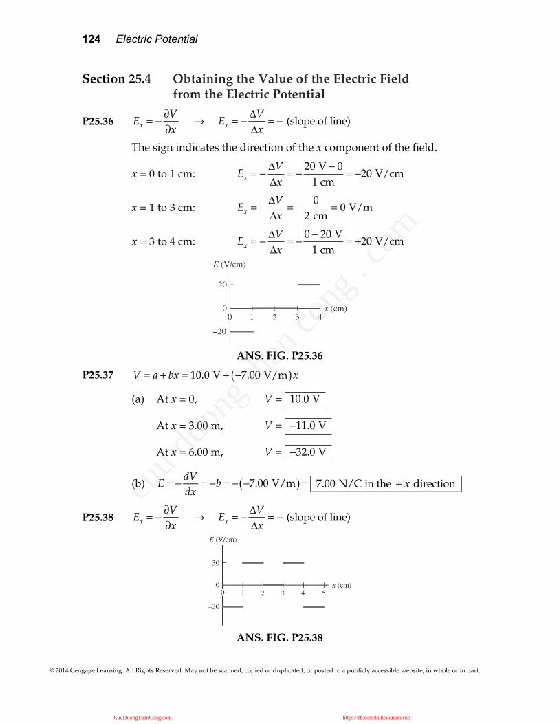
P25.36 Ex = −

∂V∂x

→ Ex = −ΔVΔx

= − (slope of line)

The sign indicates the direction of the x component of the field.

x = 0 to 1 cm: Ex = −

ΔVΔx

= −20 V − 0

1 cm= −20 V/cm

x = 1 to 3 cm: Ex = −

ΔVΔx

= −0

2 cm= 0 V/m

x = 3 to 4 cm: Ex = −

ΔVΔx

= −0 − 20 V

1 cm= +20 V/cm

ANS. FIG. P25.36

P25.37 V = a + bx = 10.0 V + −7.00 V/m( )x

(a) At x = 0, V = 10.0 V

At x = 3.00 m, V = −11.0 V

At x = 6.00 m, V = −32.0 V

(b) E = − dV

dx= −b = − −7.00 V/m( ) = 7.00 N/C in the + x direction

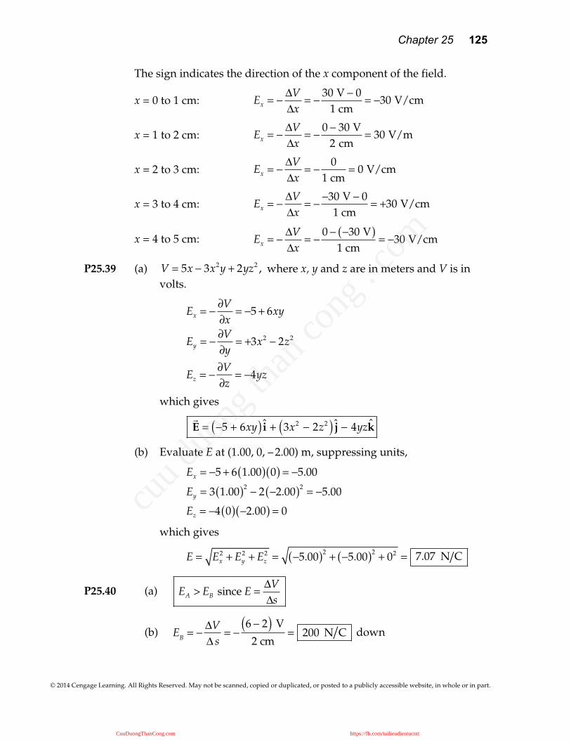
P25.38 Ex = −

∂V∂x

→ Ex = −ΔVΔx

= − (slope of line)

ANS. FIG. P25.38


cuu d

uong

than

cong

. com



Chapter 25 125


The sign indicates the direction of the x component of the field.

x = 0 to 1 cm: Ex = −

ΔVΔx

= −30 V − 0

1 cm= −30 V/cm

x = 1 to 2 cm: Ex = −

ΔVΔx

= −0 − 30 V

2 cm= 30 V/m

x = 2 to 3 cm: Ex = −

ΔVΔx

= −0

1 cm= 0 V/cm

x = 3 to 4 cm: Ex = −

ΔVΔx

= −−30 V − 0

1 cm= +30 V/cm

x = 4 to 5 cm: Ex = −

ΔVΔx

= −0 − −30 V( )

1 cm= −30 V/cm

P25.39 (a) V = 5x − 3x2y + 2yz2 , where x, y and z are in meters and V is in volts.

Ex = −∂V∂x

= −5 + 6xy

Ey = −∂V∂y

= +3x2 − 2z2

Ez = −∂V∂z

= −4yz

which gives

E = −5 + 6xy( ) i + 3x2 − 2z2( ) j − 4yzk

(b) Evaluate E at (1.00, 0, – 2.00) m, suppressing units,

Ex = −5 + 6 1.00( ) 0( ) = −5.00

Ey = 3 1.00( )2 − 2 −2.00( )2 = −5.00

Ez = −4 0( ) −2.00( ) = 0

which gives

E = Ex

2 + Ey2 + Ez

2 = −5.00( )2 + −5.00( )2 + 02 = 7.07 N C

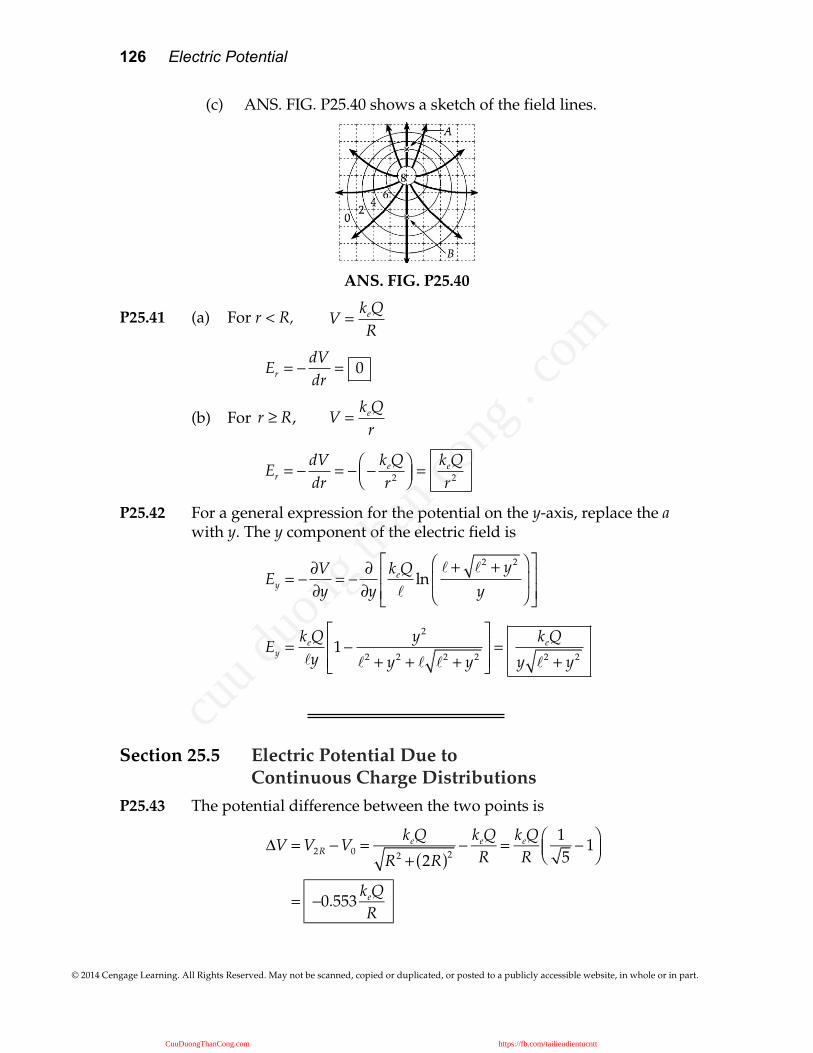
P25.40 (a)

EA > EB since E =ΔVΔs

(b) EB = −

ΔVΔ s

= −6 − 2( ) V

2 cm= 200 N C down


cuu d

uong

than

cong

. com





(c) ANS. FIG. P25.40 shows a sketch of the field lines.

ANS. FIG. P25.40

P25.41 (a) For r < R, V =

keQR

Er = −

dVdr

= 0

(b) For r ≥ R, V =

keQr

Er = −

dVdr

= − −keQr2

⎛⎝⎜

⎞⎠⎟ =

keQr2

P25.42 For a general expression for the potential on the y-axis, replace the a with y. The y component of the electric field is

Ey = −∂V∂y

= −∂∂y

keQ

ln + 2 + y2

y

⎛

⎝⎜

⎞

⎠⎟

⎡

⎣⎢⎢

⎤

⎦⎥⎥

Ey =keQy

1−y2

2 + y2 + 2 + y2

⎡

⎣⎢⎢

⎤

⎦⎥⎥=

keQ

y 2 + y2

Section 25.5 Electric Potential Due to Continuous Charge Distributions

P25.43 The potential difference between the two points is

ΔV = V2R −V0 =keQ

R2 + 2R( )2− keQ

R= keQ

R15− 1⎛

⎝⎜⎞⎠⎟

= −0.553keQR


cuu d

uong

than

cong

. com



Chapter 25 127


P25.44 V = dV∫ =

14π ∈0

dqr∫

All bits of charge are at the same distance from O. So

V =1

4π ∈0

QR

⎛⎝⎜

⎞⎠⎟ = 8.99 × 109 N ⋅m2 / C2( ) −7.50 × 10−6 C

0.140 m π⎛⎝⎜

⎞⎠⎟

= −1.51 MV

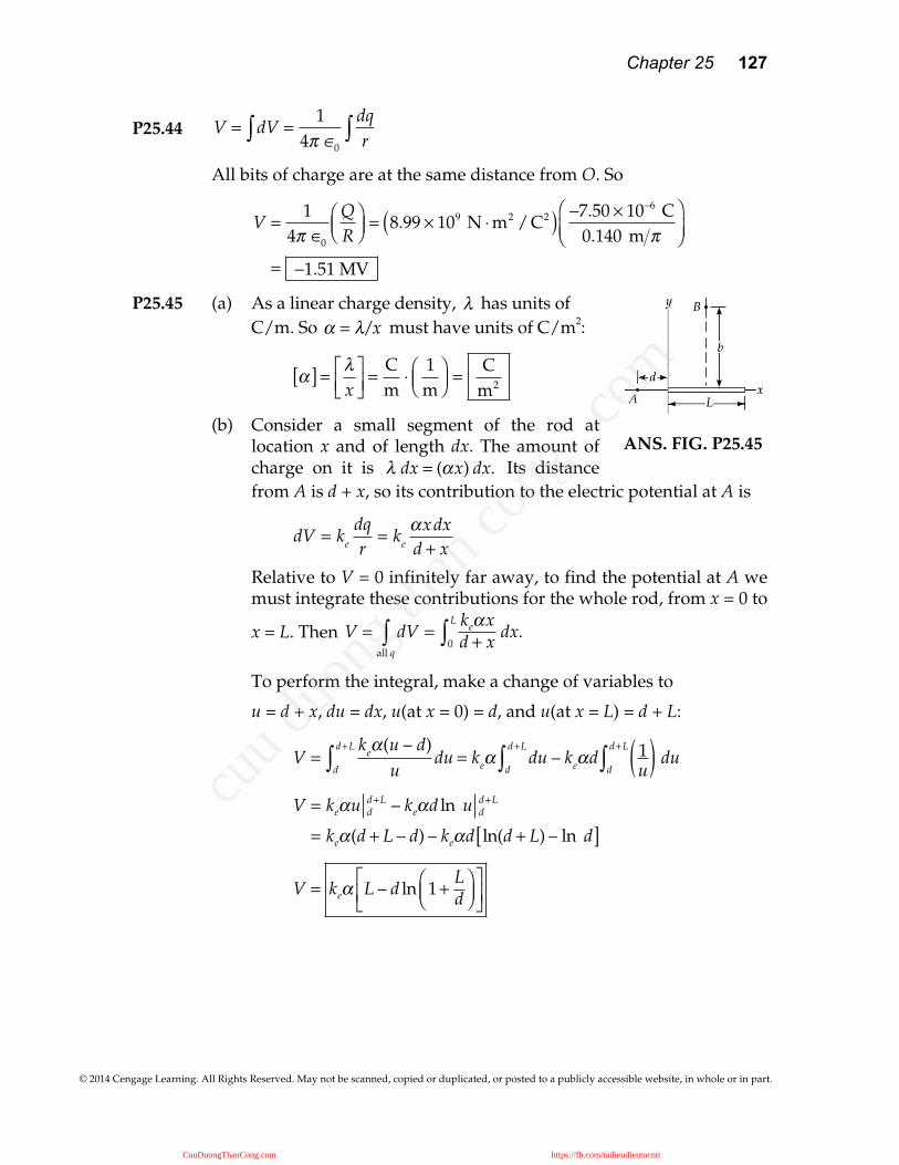
P25.45 (a) As a linear charge density, λ has units of C/m. So α = λ/x must have units of C/m2:

α[ ] = λ

x⎡⎣⎢

⎤⎦⎥=

Cm

⋅1m

⎛⎝⎜

⎞⎠⎟ =

Cm2

(b) Consider a small segment of the rod at location x and of length dx. The amount of charge on it is λ dx = (αx) dx. Its distance from A is d + x, so its contribution to the electric potential at A is

dV = ke

dqr

= ke

αxdxd + x

Relative to V = 0 infinitely far away, to find the potential at A we must integrate these contributions for the whole rod, from x = 0 to

x  = L. Then V = dV

all q∫ =

keαxd + x dx

0

L

∫ .

To perform the integral, make a change of variables to

u = d + x, du = dx, u(at x = 0) = d, and u(at x = L) = d + L:

V =

keα(u – d)ud

d+L

∫ du = keα du – d

d+L

∫ keαd 1u( )d

d+L

∫ du

V = keαu dd+L – keαd ln u d

d+L

= keα(d + L – d) – keαd ln(d + L) – ln d[ ]

V = keα L – d ln 1+

Ld

⎛⎝⎜

⎞⎠⎟

⎡⎣⎢

⎤⎦⎥

ANS. FIG. P25.45


cuu d

uong

than

cong

. com





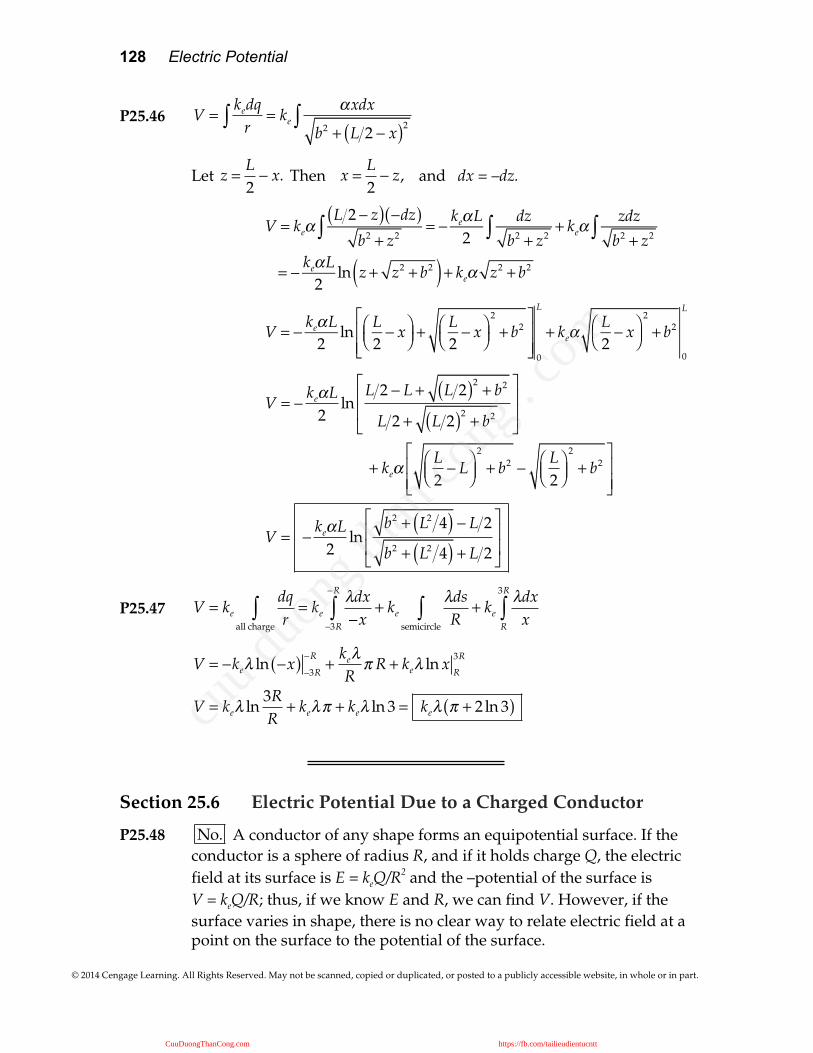
P25.46

V =kedq

r∫ = keαxdx

b2 + L 2 − x( )2∫

Let z =

L2− x. Then

x =

L2− z, and dx = –dz.

V = keαL 2 − z( ) −dz( )

b2 + z2= − keαL

2dz

b2 + z2∫ + keαzdz

b2 + z2∫∫

= − keαL2

ln z + z2 + b2( ) + keα z2 + b2

V = − keαL2

lnL2− x⎛

⎝⎜⎞⎠⎟ +

L2− x⎛

⎝⎜⎞⎠⎟

2

+ b2⎡

⎣⎢⎢

⎤

⎦⎥⎥

0

L

+ keαL2− x⎛

⎝⎜⎞⎠⎟

2

+ b2

0

L

V = −keαL

2ln

L 2 − L + L 2( )2 + b2

L 2 + L 2( )2 + b2

⎡

⎣

⎢⎢

⎤

⎦

⎥⎥

+ keαL2− L⎛

⎝⎜⎞⎠⎟

2

+ b2 −L2

⎛⎝⎜

⎞⎠⎟

2

+ b2⎡

⎣⎢⎢

⎤

⎦⎥⎥

V = −keαL

2ln

b2 + L2 4( ) − L 2

b2 + L2 4( ) + L 2

⎡

⎣

⎢⎢

⎤

⎦

⎥⎥

P25.47 V = ke

dqrall charge

∫ = keλdx−x−3R

−R

∫ + keλdsRsemicircle

∫ + keλdx

xR

3R

∫

V = −keλ ln −x( ) −3R

−R +keλR

π R + keλ ln xR

3R

V = keλ ln3RR

+ keλπ + keλ ln 3 = keλ π + 2 ln 3( )

Section 25.6 Electric Potential Due to a Charged Conductor

P25.48 No. A conductor of any shape forms an equipotential surface. If the conductor is a sphere of radius R, and if it holds charge Q, the electric field at its surface is E = keQ/R2 and the –potential of the surface is V = keQ/R; thus, if we know E and R, we can find V. However, if the surface varies in shape, there is no clear way to relate electric field at a point on the surface to the potential of the surface.


cuu d

uong

than

cong

. com



Chapter 25 129


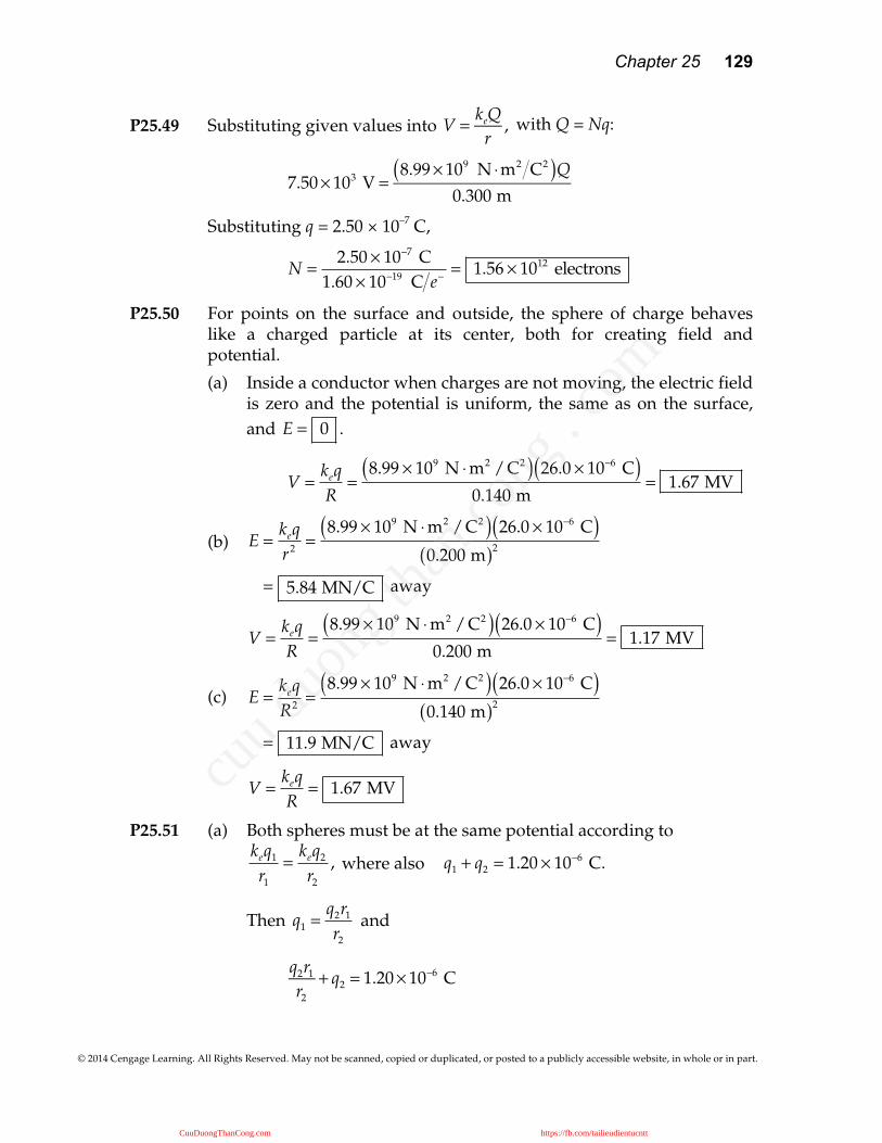
P25.49 Substituting given values into V = keQ

r, with Q = Nq:

7.50× 103 V =

8.99× 109 N ⋅m2 C2( )Q0.300 m

Substituting q = 2.50 × 10–7 C,

N =

2.50 × 10−7 C1.60 × 10−19 C e− = 1.56 × 1012 electrons

P25.50 For points on the surface and outside, the sphere of charge behaves like a charged particle at its center, both for creating field and potential.

(a) Inside a conductor when charges are not moving, the electric field is zero and the potential is uniform, the same as on the surface, and

E = 0 .

V =

keqR

=8.99 × 109 N ⋅m2 / C2( ) 26.0 × 10−6 C( )

0.140 m= 1.67 MV

(b)

E =keqr2 =

8.99 × 109 N ⋅m2 / C2( ) 26.0 × 10−6 C( )0.200 m( )2

= 5.84 MN/C away

V =

keqR

=8.99 × 109 N ⋅m2 / C2( ) 26.0 × 10−6 C( )

0.200 m= 1.17 MV

(c)

E =keqR2 =

8.99 × 109 N ⋅m2 / C2( ) 26.0 × 10−6 C( )0.140 m( )2

= 11.9 MN/C away

V =

keqR

= 1.67 MV

P25.51 (a) Both spheres must be at the same potential according to

keq1

r1

=keq2

r2

, where also q1 + q2 = 1.20 × 10−6 C.

Then q1 =

q2r1

r2

and

q2r1

r2

+ q2 = 1.20× 10−6 C


cuu d

uong

than

cong

. com





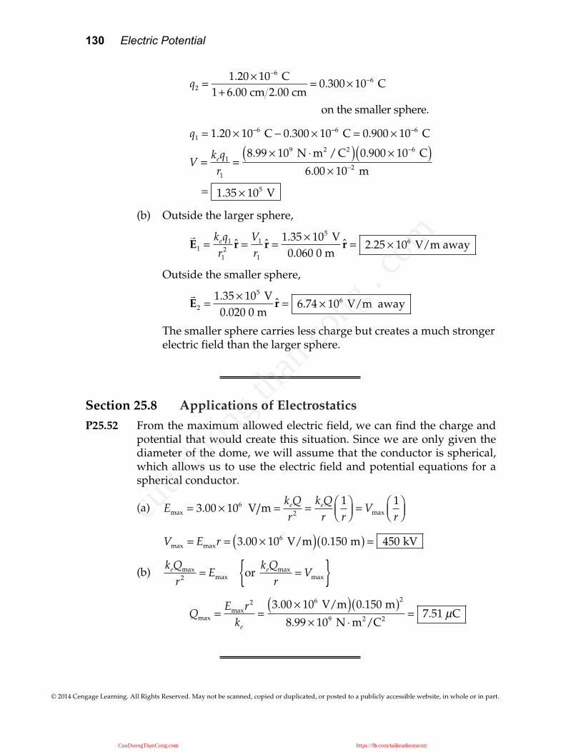
q2 =1.20× 10−6 C

1+ 6.00 cm 2.00 cm= 0.300× 10−6 C

on the smaller sphere.

q1 = 1.20 × 10−6 C − 0.300 × 10−6 C = 0.900 × 10−6 C

V =keq1

r1

=8.99 × 109 N ⋅m2 / C2( ) 0.900 × 10−6 C( )

6.00 × 10−2 m

= 1.35 × 105 V

(b) Outside the larger sphere,

E1 =

keq1

r12 r =

V1

r1

r =1.35 × 105 V

0.060 0 mr = 2.25 × 106 V/m away

Outside the smaller sphere,

E2 =

1.35 × 105 V0.020 0 m

r = 6.74 × 106 V/m away

The smaller sphere carries less charge but creates a much stronger electric field than the larger sphere.

Section 25.8 Applications of Electrostatics P25.52 From the maximum allowed electric field, we can find the charge and

potential that would create this situation. Since we are only given the diameter of the dome, we will assume that the conductor is spherical, which allows us to use the electric field and potential equations for a spherical conductor.

(a) Emax = 3.00 × 106 V m =

keQr2 =

keQr

1r

⎛⎝⎜

⎞⎠⎟ = Vmax

1r

⎛⎝⎜

⎞⎠⎟

Vmax = Emaxr = 3.00 × 106 V/m( ) 0.150 m( ) = 450 kV

(b)

keQmax

r2 = Emax or keQmax

r= Vmax{ }

Qmax =

Emaxr2

ke

=3.00 × 106 V/m( ) 0.150 m( )2

8.99 × 109 N ⋅m2/C2 = 7.51 µC


cuu d

uong

than

cong

. com



Chapter 25 131


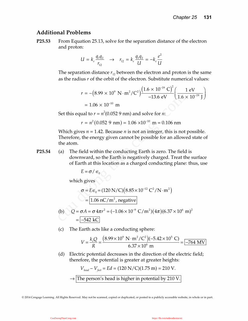
Additional Problems P25.53 From Equation 25.13, solve for the separation distance of the electron

and proton:

U = ke

q1q2

r12

→ r12 = ke

q1q2

U = −ke

e2

U

The separation distance r12 between the electron and proton is the same as the radius r of the orbit of the electron. Substitute numerical values:

r = − 8.99 × 109 N ⋅m2/C2( ) 1.6 × 10−19 C( )2

−13.6 eV1 eV

1.6 × 10−19 J⎛⎝⎜

⎞⎠⎟

= 1.06 × 10−10 m

Set this equal to r = n2(0.052 9 nm) and solve for n:

r = n2 0.052 9 nm( ) = 1.06 ×10−10 m = 0.106 nm

Which gives n = 1.42. Because n is not an integer, this is not possible. Therefore, the energy given cannot be possible for an allowed state of the atom.

P25.54 (a) The field within the conducting Earth is zero. The field is downward, so the Earth is negatively charged. Treat the surface of Earth at this location as a charged conducting plane: thus, use

E = σ/∈ 0

which gives

σ = E ∈ 0 = (120 N/C) 8.85× 10−12 C2/N ⋅m2( )= 1.06 nC/m2 , negative

(b)

Q = σA = σ 4πr2 = (−1.06 × 10−9 C/m2 ) 4π( )(6.37 × 106 m)2

= −542 kC

(c) The Earth acts like a conducting sphere:

V = keQ

R=

8.99× 109 N ⋅m2/C2( )(−5.42 × 105 C)6.37 × 106 m

= −764 MV

(d) Electric potential decreases in the direction of the electric field; therefore, the potential is greater at greater heights:

Vhead – Vfeet = Ed = (120 N/C)(1.75 m) = 210 V.

→ The person’s head is higher in potential by 210 V.


cuu d

uong

than

cong

. com





(e) Like charges repel:

FE =keq1q2

r2 =8.99 × 109 N ⋅m2/C2( )(5.42 × 105 C)2(0.273)

(3.84 × 108 m)2

FE = 4.88 × 103 N = 4.88 × 103 N away from Earth

(f) The gravitational force is

FG =GMEMM

r2

=6.67 × 10−11 N ⋅m2/kg2( )(5.98 × 1024 kg)(7.36 × 1022 kg)

(3.84 × 108 m)2

FG = 1.99 × 1020 N

Comparing the two forces,

FG

FE

=1.99 × 1020 N4.88 × 103 N

= 4.08 × 1016

The gravitational force is in the opposite direction and 4.08 × 1016

times larger. Electrical forces are negligible in accounting forplanetary motion.

P25.55 Assume the particles move along the x direction.

(a) Momentum is constant within the isolated system throughout the process. We equate it at the large-separation initial point and the point c of closest approach.

m1v1i + m2

v2 i = m1

v1c + m2

v2c

m1vi + 0 = m1v c + m2

v c

v c =

m1vm1 + m2

i =2.00 × 10−3 kg( ) 21.0 m/s( )

7.00 × 10−3 kgi = 6.00i m/s

(b) Energy is conserved within the isolated system. Compare energy terms between the large-separation initial point and the point of closest approach:

Ki +Ui = K f +U f

12

m1v1i2 +

12

m2v2 i2 + 0 =

12

m1 + m2( )vc2 +

keq1q2

rc

12

m1v2 + 0 =

12

m1 + m2( ) m1vm1 + m2

⎛⎝⎜

⎞⎠⎟

2

+keq1q2

rc


cuu d

uong

than

cong

. com



Chapter 25 133


→ m1v2 + 0 =

m12v2

m1 + m2

+ 2keq1q2

rc

→ m1 + m2( )m1v2 − m1

2v2 = 2keq1q2 m1 + m2( )

rc

m1m2v2 = 2keq1q2 m1 + m2( )

rc

rc =2keq1q2 m1 + m2( )

m1m2v2

=2 8.99 × 109 N ⋅m2/C2( ) 15.0 × 10−6 C( ) 8.50 × 10−6 C( ) 7.00 × 10−3 kg( )

2.00 × 10−3 kg( ) 5.00 × 10−3 kg( ) 21.0 m/s( )2

= 3.64 m

(c) The overall elastic collision is described by conservation of momentum:

m1v1i + m2

v2 i = m1

v1 f + m2

v2 f

m1vi + 0 = m1v1 f i + m2v2 f i

and by the relative velocity equation:

v1i − v2 i = v2 f − v1 f

v − 0 = v2 f − v1 f → v2 f = v + v1 f

We substitute the expression for v2f into the momentum equation:

m1v = m1v1 f + m2v2 f

m1v = m1v1 f + m2(v + v1 f )

m1v = m1v1 f + m2v + m2v1 f

m1v − m2v = m1v1 f + m2v1 f

m1 − m2( )v = m1 + m2( )v1 f

v1 f =m1 − m2

m1 + m2

⎛⎝⎜

⎞⎠⎟

v =2.00g − 5.00g2.00g + 5.00g

⎛⎝⎜

⎞⎠⎟

21.0 m/s( )

= −9.00 m/s

Therefore, the velocity of the particle of mass m1 is −9.00 i m/s .

(d) Substitute the expression for v1f back into v2f = v + v1f :

v2 f = v + v1 f = 21.0 m/s( ) + −9.00 m/s( ) = 12.0 m/s

Therefore, the velocity of the particle of mass m2 is 12.0 i m/s .


cuu d

uong

than

cong

. com





P25.56 Assume the particles move along the x direction.

(a) Momentum is constant within the isolated system throughout the process. We equate it at the large-separation initial point and the point c of closest approach.

m1v1i + m2

v2 i = m1

v1 f + m2

v2 f

m1vi + 0 = m1vci + m2vci → vc =m1v

m1 + m2

(b) Energy is conserved within the isolated system. Compare energy terms between the large-separation initial point and the point of closest approach:

Ki +Ui = K f +U f

12

m1v1i2 +

12

m2v2 i2 + 0 =

12

m1 + m2( )vc2 +

keq1q2

rc

12

m1v2 + 0 =

12

m1 + m2( ) m1vm1 + m2

⎛⎝⎜

⎞⎠⎟

2

+keq1q2

rc

→ m1v2 + 0 =

m12v2

m1 + m2

+ 2keq1q2

rc

→ m1 + m2( )m1v2 − m1

2v2 = 2keq1q2 m1 + m2( )

rc

m1m2v2 = 2keq1q2 m1 + m2( )

rc

→ rc =2keq1q2 m1 + m2( )

m1m2v2

(c) The overall elastic collision is described by conservation of momentum:

m1v1i + m2

v2 i = m1

v1 f + m2

v2 f

m1vi + 0 = m1v1 f i + m2v2 f i → m1v = m1v1 f + m2v2 f

and by the relative velocity equation:

v1i − v2 i = v2 f − v1 f

v − 0 = v2 f − v1 f → v2 f = v + v1 f

We substitute the expression for v2f into the momentum equation:

m1v = m1v1 f + m2v2 f

m1v = m1v1 f + m2 v + v1 f( )m1v = m1v1 f + m2v + m2v1 f


cuu d

uong

than

cong

. com



Chapter 25 135


m1v− m2v = m1v1 f + m2v1 f

m1 − m2( )v = m1 + m2( )v1 f → v1 f =m1 − m2

m1 + m2

⎛⎝⎜

⎞⎠⎟

v

Therefore, the velocity of the particle of mass m1 is

m1 − m2

m1 + m2

⎛⎝⎜

⎞⎠⎟

v i .

(d) Substitute the expression for v1f back into v2f = v + v1f :

v2 f = v + v1 f = v +m1 − m2

m1 + m2

⎛⎝⎜

⎞⎠⎟

v

=m1 + m2( ) + m1 − m2( )

m1 + m2

⎡

⎣⎢

⎤

⎦⎥v =

2m1

m1 + m2

⎛⎝⎜

⎞⎠⎟

v

Therefore, the velocity of the particle of mass m2 is

2m1

m1 + m2

⎛⎝⎜

⎞⎠⎟

v i .

P25.57 The two spheres of charge have together electric potential energy

U = qV = keq1q2

r12

= 8.99× 109 N ⋅m2/C2( ) 38( ) 54( ) 1.60× 10−19 C( )2

5.50+ 6.20( )× 10−15 m

= 4.04× 10−11 J = 253 MeV

P25.58 (a) To make a spark 5 mm long in dry air between flat metal plates requires potential difference

ΔV = Ed = 3 × 106 V/m( ) 5 × 10−3 m( ) = 1.5 × 104 V ~ 104 V

(b) The area of your skin is perhaps 1.5 m2, so model your body as a sphere with this surface area. Its radius is given by 1.5 m2 = 4π r2 , r = 0.35 m. We require that you are at the potential found in part

(a), with V =

keqr

. Then,

q =

Vrke

=1.5 × 104 V 0.35 m( )

8.99 × 109 N ⋅m2 / C2

JV ⋅C

⎛⎝⎜

⎞⎠⎟

N ⋅mJ

⎛⎝⎜

⎞⎠⎟

q = 5.8 × 10−7 C ~ 10−6 C


cuu d

uong

than

cong

. com





P25.59 We have V1 = keQ/R = 200 V and V2 = keQ/(R + 10 cm) = 150 V.

(a)

V1

V2

=R + 10 cm

R=

200150

→ 150 R + 10 cm( ) = 200R → R = 30.0 cm

(b) From V1 = ke

QR

, we have

Q = V1R

ke

= 200 V( ) 0.300 m( )8.99× 109 N ⋅m2/C2 = 6.67 × 10−9 C = 6.67 nC

(c) We have V = keQ/R = 210 V and E = keQ/(R + 10 cm)2 = 400 V/m. Therefore,

VE

=R + 10 cm( )2

R=

210400

=2140

→ 40 R + 0.100( )2 = 21R

where R is in meters.

Thus, we have

40R2 + 8R + 0.4 = 21R → 40R2 – 13R + 0.4 = 0

There are two possibilities, according to

R =

+13 ± 132 − 4(40) 0.4( )80

= either 0.291 m or 0.034 4 m

= 29.1 cm or 3.44 cm

(d) If the radius is 29.1 cm,

Q =

VRke

=210 V( ) 0.291 m( )

8.99 × 109 N ⋅m2/C2 = 6.79 × 10−9 C = 6.79 nC

If the radius is 3.44 cm,

Q =

VRke

=210 V( ) 0.0344 m( )

8.99 × 109 N ⋅m2/C2 = 8.04 × 10−10 C = 804 pC

(e) No; two answers exist for each part.

P25.60 (a) The exact potential is

+

keqr + a

−keq

r − a= +

keq3a + a

−keq

3a − a=

keq4a

−2keq4a

= −keq4a

(b) The approximate expression –2keqa/x2 gives

–2keqa/(3a)2 = –keq/4.5a


cuu d

uong

than

cong

. com



Chapter 25 137


Compare the exact to the approximate solution:

1/ 4 − 1/ 4.51/ 4

=0.54.5

= 0.111 .

The approximate expression − 2keqa/x2 gives − keq/4.5a, which is different by only 11.1%.

P25.61 W = Vdq

0

Q

∫ , where V =

keqR

.

Therefore, W =

keQ2

2R=

8.99 × 109 N ⋅m2/C2( ) 125 × 10−6 C( )2

2 0.100 m( ) = 702 J .

P25.62 W = Vdq

0

Q

∫ , where V =

keqR

. Therefore, W =

keQ2

2R.

P25.63 For a charge at (x = –1 m, y = 0), the radial distance away is given by

(x + 1)2 + y2 . So the first term will be the potential it creates if

(8.99 × 109 N ⋅ m2/C2)Q1 = 36 V⋅m → Q1 = 4.00 nC

The second term is the potential of a charge at (x = 0, y = 2 m) with

(8.99 × 109 N ⋅ m2/C2)Q2 = –45 V⋅m → Q2 = –5.01 nC

Thus we have 4.00 nC at ( − 1.00 m, 0) and − 5.01 nC at (0, 2.00 m).

P25.64 From Example 25.5, the potential along the x axis of a ring of charge of radius R is

V =

keQ

R2 + x2

Therefore, the potential at the center of the ring is

V =

keQ

R2 + 0( )2 =

keQR

When we place the point charge Q at the center of the ring, the electric potential energy of the charge–ring system is

U = QV = Q

keQR

⎛⎝⎜

⎞⎠⎟ =

keQ2

R

Now, apply Equation 8.2 to the isolated system of the point charge and the ring with initial configuration being that with the point charge at the center of the ring and the final configuration having the point


cuu d

uong

than

cong

. com





charge infinitely far away and moving with its highest speed:

ΔK + ΔU = 0 →

12

mvmax2 − 0⎛

⎝⎜⎞⎠⎟ + 0 − keQ

2

R⎛⎝⎜

⎞⎠⎟ = 0

Solve for the maximum speed:

vmax =

2keQ2

mR⎛⎝⎜

⎞⎠⎟

1 / 2

Substitute numerical values:

vmax =2 8.99 × 109 N ⋅m2/C2( ) 50.0 × 10−6 C( )2

0.100 kg( ) 0.500 m( )⎛

⎝⎜⎜

⎞

⎠⎟⎟

1/2

= 30.0 m/s

Therefore, even if the charge were to accelerate to infinity, it would only achieve a maximum speed of 30.0 m/s, so it cannot strike the wall of your laboratory at 40.0 m/s.

P25.65 In Equation 25.3, V2 – V1 = ΔV = –

E ⋅ ds

1

2

∫ , think about stepping from

distance r1 out to the larger distance r2 away from the charged line. Then d

s = drr, and we can make r the variable of integration:

V2 – V1 = – λ

2π ∈0 r

r1

r2∫ r ⋅ dr r with r ⋅ r = 1 ⋅ 1cos0 = 1

The potential difference is

V2 – V1 = – λ

2π ∈0

drrr1

r2∫ = – λ2π ∈0

ln rr1

r2

and V2 – V1 = – λ

2π ∈0ln r2 – ln r1( ) = – λ

2π ∈0ln r2

r1

P25.66 (a) Modeling the filament as a single charged particle, we obtain

V = keQ

r=

8.99 × 109 N ⋅m2/C2( ) 1.60 × 10−9 C( )2.00 m

= 7.19 V

(b) Modeling the filament as two charged particles, we obtain

V = keQ1

r1

+ keQ2

r2

= keQ1

r1

+ Q2

r2

⎛⎝⎜

⎞⎠⎟

= 8.99 × 109 N ⋅m2/C2( ) 0.800 × 10−9 C1.50 m

+ 0.800 × 10−9 C2.50 m

⎛⎝⎜

⎞⎠⎟

= 7.67 V


cuu d

uong

than

cong

. com



Chapter 25 139


(c) Modeling the filament as four charged particles, we obtain

V = keQ1

r1

+ Q2

r2

+ Q3

r3

+ Q4

r4

⎛⎝⎜

⎞⎠⎟

= 8.99 × 109 N ⋅m2/C2( ) × 0.400 × 10−9 C

1.25 m+ 0.400 × 10−9 C

1.75 m⎛⎝⎜

+ 0.400 × 10−9 C2.25 m

+ 0.400 × 10−9 C2.75 m

⎞⎠⎟

= 7.84 V

(d) We represent the exact result as

V = keQ

ln+ a

a⎛⎝⎜

⎞⎠⎟

=8.99 × 109 N ⋅m2/C2( ) 1.60 × 10−9 C( )

2.00 m

⎡

⎣⎢⎢

⎤

⎦⎥⎥ln

31

⎛⎝⎜

⎞⎠⎟

= 7.901 2 V

Modeling the line as a set of points works nicely. The exact result, represented as 7.90 V, is approximated to within 0.8% by the four-particle version.

P25.67 We obtain the electric potential at P by integrating:

V = keλdxx2 + b2

a

a+L

∫ = keλ ln x + x2 + b2( )⎡⎣

⎤⎦ a

a+L

= keλ lna + L+ a + L( )2 + b2

a + a2 + b2

⎡

⎣⎢⎢

⎤

⎦⎥⎥

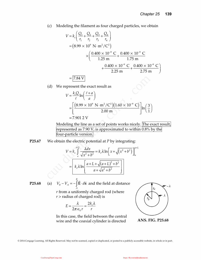
P25.68 (a) VB −VA = −

E ⋅ds

A

B

∫ and the field at distance

r from a uniformly charged rod (where r > radius of charged rod) is

E = λ

2π∈0 r= 2keλ

r

In this case, the field between the central wire and the coaxial cylinder is directed ANS. FIG. P25.68


cuu d

uong

than

cong

. com





perpendicular to the line of charge so that

VB −VA = −

2keλr

drra

rb

∫ = 2keλ lnra

rb

⎛⎝⎜

⎞⎠⎟

or

ΔV = 2keλ ln

ra

rb

⎛⎝⎜

⎞⎠⎟

.

(b) From part (a), when the outer cylinder is considered to be at zero potential, the potential at a distance r from the axis is

V = 2keλ ln

ra

r⎛⎝⎜

⎞⎠⎟

The field at r is given by

E = −

∂V∂r

= −2keλrra

⎛⎝⎜

⎞⎠⎟

−ra

r2⎛⎝⎜

⎞⎠⎟ =

2keλr

But, from part (a), 2keλ =

ΔVln ra rb( ) .

Therefore,

E =ΔV

ln ra rb( )1r

⎛⎝⎜

⎞⎠⎟ .

P25.69 (a) The positive plate by itself creates a field

E = σ

2∈0

= 36.0× 10−9 C m2

2 8.85× 10−12 C2 N ⋅m2( ) = 2.03 kN C

away from the positive plate. The negative plate by itself creates the same size field and between the plates it is in the same direction. Together the plates create a uniform field

4.07 kN C

in the space between.

(b) Take V = 0 at the negative plate. The potential at the positive plate is then

ΔV = V − 0 = − Exdx

xi

x f

∫ = − −4.07 kN C( )dx0

12.0 cm

∫

The potential difference between the plates is

V = 4.07 × 103 N C( ) 0.120 m( ) = 488 V

(c) The positive proton starts from rest and accelerates from higher to lower potential. Taking Vi = 488 V and Vf = 0, by energy


cuu d

uong

than

cong

. com



Chapter 25 141


conservation, we find the proton’s final kinetic energy.

K + qV( )i

= K + qV( ) f→ K f = qVi

12

mv2 + qV⎛⎝⎜

⎞⎠⎟ i

=12

mv2 + qV⎛⎝⎜

⎞⎠⎟ f

qVi = 1.60 × 10−19 C( ) 488 V( ) = 1

2mv f

2 = 7.81× 10−17 J

(d) From the kinetic energy of part (c),

K =12

mv f2

v f =2Km

=2 7.81× 10−17 J( )1.67 × 10−27 kg

= 3.06 × 105 m/s = 306 km/s

(e) Using the constant-acceleration equation, v f

2 = vi2 + 2a x f − xi( ) ,

a =v f

2 − vi2

2 x f − xi( ) =3.06× 105 m/s( )2

− 02 0.120 m( )

= 3.90× 1011 m/s2 toward the negative plate

(f) The net force on the proton is given by Newton’s second law:

F∑ = ma = 1.67 × 10−27 kg( ) 3.90× 1011 m/s2( )= 6.51× 10−16 N toward the negative plate

(g) The magnitude of the electric field is

E =

Fq=

6.51× 10−16 N1.60 × 10−19 C

= 4.07 kN C

(h) They are the same.

P25.70 (a) Inside the sphere, Ex = Ey = Ez = 0 .

(b) Outside,

Ex = − ∂V∂x

= − ∂∂x

V0 −E0z +E0a3z x2 + y2 + z2( )−3 2( )

= − 0+ 0+E0a3z − 3

2⎛⎝⎜

⎞⎠⎟ x2 + y2 + z2( )−5 2

2x( )⎡⎣⎢

⎤⎦⎥

Ex = 3E0a3xz x2 + y2 + z2( )−5 2


cuu d

uong

than

cong

. com





Ey = − ∂V∂y

= − ∂∂y

V0 −E0z +E0a3z x2 + y2 + z2( )−3 2( )

= −E0a3z − 3

2⎛⎝⎜

⎞⎠⎟ x2 + y2 + z2( )−5 2

2y

Ey = 3E0a3yz x2 + y2 + z2( )−5 2

Ez = − ∂V∂z

= − ∂∂z

V0 −E0z +E0a3z x2 + y2 + z2( )−3 2⎡

⎣⎤⎦

= E0 −E0a3z − 3

2⎛⎝⎜

⎞⎠⎟ x2 + y2 + z2( )−5 2

2z( )−E0a3 x2 + y2 + z2( )−3 2

Ez = E0 +E0a3 2z2 − x2 − y2( ) x2 + y2 + z2( )−5 2

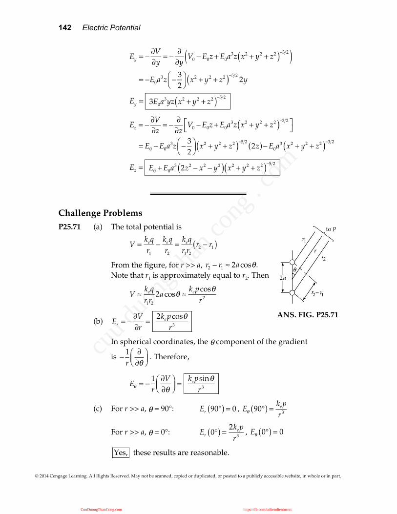
Challenge Problems P25.71 (a) The total potential is

V =

keqr1

−keqr2

=keqr1r2

r2 − r1( )

From the figure, for r >> a, r2 − r1 ≈ 2acosθ. Note that r1 is approximately equal to r2. Then

V ≈

keqr1r2

2acosθ ≈kepcosθ

r2

(b) Er = −

∂V∂r

=2kepcosθ

r3

In spherical coordinates, the θ component of the gradient

is −

1r

∂∂θ

⎛⎝⎜

⎞⎠⎟

. Therefore,

Eθ = −

1r

∂V∂θ

⎛⎝⎜

⎞⎠⎟=

kepsinθr3

(c) For r >> a, θ = 90°: Er 90°( ) = 0 , Eθ 90°( ) = kep

r3

For r >> a, θ = 0°: Er 0°( ) = 2kep

r3 , Eθ 0°( ) = 0

Yes, these results are reasonable.

ANS. FIG. P25.71


cuu d

uong

than

cong

. com



Chapter 25 143


(d) No, because as r → 0, E → ∞. The magnitude of the electric field between the charges of the dipole is not infinite.

(e) Substituting r1 ≈ r2 ≈ r = (x2 + y2 )1/2 and cos θ =

y

x2 + y2( )1/2 into

V =

kep cosθr2 gives

V =kepy

x2 + y2( )3 2 .

(f)

Ex = −∂V∂x

=3kepxy

x2 + y2( )5 2 and

Ey = −∂V∂y

=kep 2y2 − x2( )

x2 + y2( )5 2

P25.72 Following the problem’s suggestion, we use dU = Vdq, where the

potential is given by V =

keqr

. The element of charge in a shell is

dq = ρ (volume element) or dq = ρ 4π r2dr( ) and the charge q in a sphere of radius r is

q = 4πρ r2dr

0

r

∫ = ρ4π r3

3⎛⎝⎜

⎞⎠⎟

Substituting this into the expression for dU, we have

dU =keqr

⎛⎝⎜

⎞⎠⎟ dq = keρ

4π r3

3⎛⎝⎜

⎞⎠⎟

1r

⎛⎝⎜

⎞⎠⎟ ρ 4π r2dr( ) = ke

16π 2

3⎛⎝⎜

⎞⎠⎟ρ2r4dr

U = dU∫ = ke16π 2

3⎛⎝⎜

⎞⎠⎟ρ2 r4dr

0

R

∫ = ke16π 2

15⎛⎝⎜

⎞⎠⎟ρ2R5

But the total charge, Q = ρ 4

3π R3 . Therefore,

U =

35

keQ2

R.

P25.73 For an element of area which is a ring of radius r and width dr, the

incremental potential is given by dV =

kedq

r2 + x2, where

dq = σdA = Cr 2π rdr( )

The electric potential is then given by

V = C 2π ke( ) r2dr

r2 + x20

R

∫


cuu d

uong

than

cong

. com





From a table of integrals,

r2drr2 + x2∫ = r

2r2 + x2 − x2

2ln r + r2 + x2( )

The potential then becomes, after substituting and rearranging,

V = C 2π ke( ) r2drr2 + x2

0

R

∫

= π keC R R2 + x2 + x2 lnx

R + R2 + x2

⎛⎝⎜

⎞⎠⎟

⎡

⎣⎢

⎤

⎦⎥

P25.74 Take the illustration presented with the problem as an initial picture. No external horizontal forces act on the set of four balls, so its center of mass stays fixed at the location of the center of the square. As the charged balls 1 and 2 swing out and away from each other, balls 3 and 4 move up with equal y-components of velocity. The maximum-kinetic-energy point is illustrated. System energy is conserved because it is isolated:

Ki +Ui = K f +U f

0 +Ui = K f +U f

→Ui = K f +U f

keq2

a=

12

mv2 +12

mv2 +12

mv2 +12

mv2 +keq

2

3a

2keq2

3a= 2mv2 → v =

keq2

3am

P25.75 (a) Take the origin at the point where we will find the potential. One

ring, of width dx, has charge

Qdxh

and, according to Example

25.5, creates potential

dV =

keQdx

h x2 + R2

The whole stack of rings creates potential

V = dVall charge∫ =

keQdx

h x2 + R2d

d+h

∫ =keQh

ln x + x2 + R2( )d

d+h

=keQh

lnd + h + d + h( )2 + R2

d + d2 + R2

⎛

⎝⎜⎜

⎞

⎠⎟⎟

ANS. FIG. P25.74


cuu d

uong

than

cong

. com



Chapter 25 145


(b) A disk of thickness dx has charge

Qdxh

and charge-per-area

Qdxπ R2h

. According to Example 25.6, it creates potential

dV = 2π ke

Qdxπ R2h

x2 + R2 − x( )

Integrating,

V = 2keQR2h

x2 + R2 dx − xdx( )d

d+h

∫

= 2keQR2h

12

x x2 + R2 + R2

2ln x + x2 + R2( )− x2

2⎡⎣⎢

⎤⎦⎥d

d+h

V =

keQR2h

d + h( ) d + h( )2 + R2 − d d2 + R2⎡⎣⎢

− 2dh− h2 + R2 lnd + h+ d + h( )2 + R2

d + d2 + R2

⎛

⎝⎜⎜

⎞

⎠⎟⎟

⎤

⎦⎥⎥

P25.76 The plates create a uniform electric field to the right in the picture, with magnitude

V0 − −V0( )d

= 2V0

d

Assume the ball swings a small distance x to the right so that the thread is at angle θ from the vertical. The ball moves to a place where the voltage created by the plates is lower by

−Ex = −

2V0

dx

Because its ground connection maintains the ball at V = 0, charge q flows from ground onto the ball, so that

− 2V0x

d+ keq

R= 0 → q = 2V0xR

ked

Then the ball feels an electric force

F = qE =

4V02xR

ked2


cuu d

uong

than

cong

. com





to the right. For equilibrium, the electric force must be balanced by the horizontal component of string tension according to

T sinθ = qE =

4V02xR

ked2

and the weight of the ball must be balanced by the vertical component of string tension according to T cosθ = mg. Dividing the expression for the horizontal component by that for the vertical component, we find that

tanθ = 4V0

2xRked

2mg

For very small angles, we can approximate tanθ sinθ = x

L, so the

above expression becomes

xL= 4V0

2xRked

2mg → V0 =

ked2mg

4RL⎛⎝⎜

⎞⎠⎟

1 2

for small x

If V0 is less than this value, the only equilibrium position of the ball is hanging straight down. If V0 exceeds this value, the ball will swing over to one plate or the other.

P25.77 For the given charge distribution,

V x, y, z( ) = ke q( )

r1

+ke −2q( )

r2

where r1 = x + R( )2 + y2 + z2

and r2 = x2 + y2 + z2

The surface on which V (x, y, z) = 0 is given by

keq

1r1

−2r2

⎛⎝⎜

⎞⎠⎟= 0 or 2r1 = r2

This gives:

4 x + R( )2 + 4y2 + 4z2 = x2 + y2 + z2

which may be written in the form:

x2 + y2 + z2 +

83

R⎛⎝⎜

⎞⎠⎟ x + 0( )y +

0( )z + 4

3R2⎛

⎝⎜⎞⎠⎟ = 0 [1]


cuu d

uong

than

cong

. com



Chapter 25 147


The general equation for a sphere of radius a centered at (x0, y0, z0) is:

x − x0( )2 + y − y0( )2 + z − z0( )2 − a2 = 0

or

x2 + y2 + z2 + −2x0( )x + −2y0( )y + −2z0( )z + x0

2 + y02 + z0

2 − a2( ) = 0

[2]

Comparing equations [1] and [2], it is seen that the equipotential surface for which V = 0 is indeed a sphere and that:

−2x0 =

83

R; − 2y0 = 0; − 2z0 = 0; x02 + y0

2 + z02 − a2 = 4

3R2

Thus, x0 = −

43

R , y0 = z0 = 0 , and a2 =

169

−43

⎛⎝⎜

⎞⎠⎟ R2 =

49

R2

The equipotential surface is therefore a sphere centered at

−

43

R, 0, 0⎛⎝⎜

⎞⎠⎟ , having a radius

23

R .


cuu d

uong

than

cong

. com





ANSWERS TO EVEN-NUMBERED PROBLEMS P25.2 (a) –6.00 × 10–4 J; (b) –50.0 V

P25.4 1.35 MJ

P25.6 See P25.6 for full explanation.

P25.8 (a) –2.31 kV; (b) Because a proton is more massive than an electron, a proton traveling at the same speed as an electron has more initial kinetic energy and requires a greater magnitude stopping potential; (c)

ΔVp ΔVe = −mp me

P25.10 (a) isolated; (b) electric potential energy and elastic potential energy;

(c)

2QEk

; (d) Particle in equilibrium; (e)

QEk

; (f)

d2 ′xdt2 = −

k ′xm

;

(g) 2π m

k; (h) The period does not depend on the electric field. The

electric field just shifts the equilibrium point for the spring, just like a gravitational field does for an object hanging from a vertical spring.

P25.12 (a) –5.76 × 10–7 V; (b) 3.84 × 10–7 V; (c) Because the charge of the proton has the same magnitude as that of the electron, only the sign of the answer to part (a) would change.

P25.14 (a) 5.39 kV; (b) 10.8 kV

P25.16 (a) 103 V; (b) −3.85 × 10−7 J, positive work must be done

P25.18 (a) 5.43 kV; (b) 6.08 kV; (c) 658 V

P25.20 (a) 6.00 m; (b) –2.00 µC

P25.22 –11.0 × 107 V

P25.24 5.41

keQ2

s

P25.26 (a)

2

x / a( )2 + 1; (b) See ANS. FIG. P25.26(b).

P25.28 (a) no point; (b)

2keqa

P25.30 ΔEint =

5keq2

9d


cuu d

uong

than

cong

. com



Chapter 25 149


P25.32 (a) v1 =

2m2keq1q2

m1 m1 + m2( )1

r1 + r2

−1d

⎛⎝⎜

⎞⎠⎟

and v2 =

2m1keq1q2

m2 m1 + m2( )1

r1 + r2

−1d

⎛⎝⎜

⎞⎠⎟

; (b) faster than calculated in (a)

P25.34 v = 1+

18

⎛⎝⎜

⎞⎠⎟

keq2

mL

P25.36 See ANS. FIG. P25.36.

P25.38 See ANS. FIG. P25.38.

P25.40 (a) EA > EB since E =

ΔVΔs

; (b) 200 N/C; (c) See ANS. FIG. P25.40.

P25.42 Ey =

keQy 2 + y2

P25.44 –1.51 MV

P25.46

− keαL2

lnb2 + L2 4( ) − L 2

b2 + L2 4( ) + L 2

⎡

⎣

⎢⎢

⎤

⎦

⎥⎥

P25.48 No. A conductor of any shape forms an equipotential surface. However, if the surface varies in shape, there is no clear way to relate electric field at a point on the surface to the potential of the surface.

P25.50 (a) 0, 1.67 MV; (b) 5.84 MN/C away, 1.17 MV; (c) 11.9 MN/C away, 1.67 MV

P25.52 (a) 450 kV; 7.51 µC

P25.54 (a) 1.06 nC/m2, negative; (b) –542 kC; (c) –764 MV; (d) The person’s head is higher in potential by 210 V; (e) 4.88 × 103 N away from Earth; (f) The gravitational force is in the opposite direction and 4.08 × 1016

times larger. Electrical forces are negligible in accounting for planetary motion.

P25.56 (a)

m1vm1 + m2

; (b)

2keq1q2 m1 + m2( )m1m2v2 ; (c)

m1 − m2

m1 + m2

⎛⎝⎜

⎞⎠⎟

v i; (d)

2m1

m1 + m2

⎛⎝⎜

⎞⎠⎟

v i

P25.58 (a) ~104 V; (b) ~10–6 C

P25.60 (a) −

keq4a

; (b) The approximate expression –2keqa/x2 gives –keq/4.5,

which is different by only 11.1%.


cuu d

uong

than

cong

. com





P25.62

keQ2

2R

P25.64 Even if the charge were to accelerate to infinity, it would only achieve a maximum speed of 30.0 m/s, so it cannot strike the wall of your laboratory at 40.0 m/s.

P25.66 (a) 7.19 V; (b) 7.67 V; (c) 7.84 V; (d) The exact result, represented as 7.90 V, is approximated to within 0.8% by the four-particle version.

P25.68 (a) ΔV = 2keλ ln

ra

rb

⎛⎝⎜

⎞⎠⎟

; (b) E =

ΔVln ra rb( )

1r

⎛⎝⎜

⎞⎠⎟

P25.70 (a) Ex = Ey = Ez = 0; (b) Ex =3E0a3xz x2 + y2 + z2( )−5 2

,

Ey = 3E0a3yz x2 + y2 + z2( )−5 2

, Ez = E0 +E0a3 2z2 − x2 − y2( ) x2 + y2 + z2( )−5 2

P25.72 U =

35

keQ2

R

P25.74 v =

keq2

3am

P25.76 See P25.76 for full explanation.


cuu d

uong

than

cong

. com



vật lý 2,dhspkthcm

Documents