Gabriel M. Ahlfeldt and Alexandra Mastro Valuing iconic design: Frank Lloyd Wright architecture in Oak Park, Illinois Article (Accepted version) (Refereed) Original citation: Ahlfeldt, Gabriel M. and Mastro, Alexandra (2012) Valuing iconic design: Frank Lloyd Wright architecture in Oak Park, Illinois. Housing studies, 27 (8). pp. 1079-1099. ISSN 0267-3037 DOI: 10.1080/02673037.2012.728575 © 2012 Taylor & Francis This version available at: http://eprints.lse.ac.uk/43470/ Available in LSE Research Online: July 2013 LSE has developed LSE Research Online so that users may access research output of the School. Copyright © and Moral Rights for the papers on this site are retained by the individual authors and/or other copyright owners. Users may download and/or print one copy of any article(s) in LSE Research Online to facilitate their private study or for non-commercial research. You may not engage in further distribution of the material or use it for any profit-making activities or any commercial gain. You may freely distribute the URL (http://eprints.lse.ac.uk) of the LSE Research Online website. This document is the author’s final accepted version of the journal article. There may be differences between this version and the published version. You are advised to consult the publisher’s version if you wish to cite from it.

Welcome message from author
This document is posted to help you gain knowledge. Please leave a comment to let me know what you think about it! Share it to your friends and learn new things together.
Transcript

Gabriel M. Ahlfeldt and Alexandra Mastro
Valuing iconic design: Frank Lloyd Wright architecture in Oak Park, Illinois Article (Accepted version) (Refereed)
Original citation:
Ahlfeldt, Gabriel M. and Mastro, Alexandra (2012) Valuing iconic design: Frank Lloyd Wright architecture in Oak Park, Illinois. Housing studies, 27 (8). pp. 1079-1099. ISSN 0267-3037
DOI: 10.1080/02673037.2012.728575 © 2012 Taylor & Francis This version available at: http://eprints.lse.ac.uk/43470/ Available in LSE Research Online: July 2013 LSE has developed LSE Research Online so that users may access research output of the School. Copyright © and Moral Rights for the papers on this site are retained by the individual authors and/or other copyright owners. Users may download and/or print one copy of any article(s) in LSE Research Online to facilitate their private study or for non-commercial research. You may not engage in further distribution of the material or use it for any profit-making activities or any commercial gain. You may freely distribute the URL (http://eprints.lse.ac.uk) of the LSE Research Online website. This document is the author’s final accepted version of the journal article. There may be differences between this version and the published version. You are advised to consult the publisher’s version if you wish to cite from it.
1
Valuing Iconic Design:
Frank Lloyd Wright Architecture in Oak Park, Illinois
Gabriel M. Ahlfeldt*
Alexandra Mastro
London School of Economics
Forthcoming in Housing Studies
Abstract: This study investigates the willingness of homebuyers to pay for co-location with iconic architecture.
Oak Park, Illinois was chosen as the study area given its unique claim of having 24 residential structures
designed by world-famous American architect Frank Lloyd Wright, in addition to dozens of other designated
landmarks and three preservation districts. This study adds to the limited body of existing literature on the
external price effects of architectural design and is unique in its focus on residential architecture. We find a
premium of about 8.5% within 50-100m of the nearest Wright building and about 5% within 50-250m. These
results indicate that an external premium to iconic architecture does exist, although it may partially be
attributable to the prominence of the architect.
Keywords: Frank Lloyd Wright, hedonic analysis, iconic architecture, property prices
JEL: R21, Z11
* DEPARTMENT OF GEOGRAPHY AND ENVIRONMENT AND SERC, HOUGHTON STREET | LONDON WC2A 2AE, [email protected],WWW.AHLFELDT.COM
2
1. Introduction
While the built environment plays a significant role in the overall appeal of a neighbourhood,
few studies have tried to quantify the external effects of high quality design. This study will
contribute to the limited body of research on the subject and consider the premium achieved
by houses in the vicinity of iconic architecture. The results of this study should be of interest
to local governments and communities who could use the development of iconic structures to
increase the appeal and prestige of their areas. In addition, a positive result would show that
the preservation of architecturally significant buildings can be warranted.
There are two major challenges faced by researchers conducting empirical analyses on the
value of architecture; first, since a certain architectural design or style may be liked by some
and not by others, it is difficult to determine explicitly what constitutes ‘good’ design; and
second, many of the most significant architectural designs are found in public buildings such
as stadia or museums and in these cases the benefit of the architectural element cannot be
isolated from the use of the building. This study circumvents both of these issues by focusing
on residential properties designed by a well-known architect, Frank Lloyd Wright.
While the current media culture has given rise to many famous architects such as Frank
Gehry, Zaha Hadid, and Shigeru Ban (to name just a few), who are known for their
distinctive designs, Frank Lloyd Wright occupies a unique position among the general
populace in terms of their familiarity with both his name and his architectural style. In a
national survey in 1991 the American Institute of Architects named Wright the “greatest
American architect of all time” (Brewster, 2004). His overwhelming popularity permits this
study to proceed under the assumption that his designs are considered architecturally
significant and add prestige to the neighbourhoods in which they are located. In addition,
unlike many architects who became well-known for large public projects, Wright was
primarily a residential architect. This allows for the separation of design and use since the
subject properties are privately owned and the only benefit to outsiders is their exterior
appearance. Oak Park, Illinois provides a unique case study for empirical research as Wright
built 24 homes in the village between 1892 and 1914.
Wright’s designs are considered by many to be works of art. Residents are likely to benefit
both from the added prestige of being located near a Wright home and also from the view as
they are likely to pass by the home regularly. As long as homebuyers acknowledge these

3
benefits and bid up the prices of houses near Wright houses, the benefit will be capitalised in
property prices. To assess whether such a premium exists, we conducted a spatial hedonic
property price analysis, guided by a simple bid-rent model. Previewing our findings, the
study will conclude that an external premium to iconic architecture does exist and that the
effect steeply decays with distance. In addition, significant benefits were found to be
associated with location in one of the designated preservation districts as well as proximity
to designated landmarks more generally. These results should be of interest to local and
national governments and communities as they illustrate the potential for promoting the
attractiveness and desirability of local areas through iconic architecture.
2. Frank Lloyd Wright and the Prairie Architectural Style
Frank Lloyd Wright was born in Wisconsin in 1867 and spent most of his early years in
Madison. He did not formally train as an architect but instead completed two semesters of
civil engineering before moving to Chicago in 1887. In Chicago, he worked directly under
Louis Sullivan, a prominent architect at that time, and was greatly influenced by Sullivan’s
strong belief that form should follow function and that American architecture should not be
overly influenced by European styles. In 1893 Wright started his own practice in Chicago,
but in 1898 he relocated to a studio attached to his home in Oak Park, a suburb directly west
of Chicago. Wright was at the forefront of the uniquely American Prairie architecture
movement which was based on the idea that a structure should be designed to fit with its
natural surroundings. The Prairie architects “rejected the historic styles because they, like
many of their predecessors in the nineteenth century, believed themselves to be living in a
new cultural age whose architecture deserved an aesthetic expression of its own” (Sprague,
1986, p. 7).
The Prairie style is characterised by strong horizontal lines, geometric shapes and a lack of
ornamentation. The materials used – including wood, stucco, brick and concrete – were
never painted and therefore retained a natural appearance. Gently sloping roofs, deep
overhangs and rows of small windows are typical design features. Geometric stained glass
windows are a unique feature that defines many of Wright’s buildings.
Between 1892 and 1914, Frank Lloyd Wright completed several homes in Oak Park for
prominent Chicago families. There are 24 properties in total, 23 of which (excluding 400 S
Home Street) are located in close proximity to each other as shown in Figure 1. The homes
are all privately owned with the exception of Wright’s home and studio which is open to the
public. While this study is not focused on the internal price premiums achieved by Wright
4
houses, five properties sold between 2003 and 2009 at a statistically significant 41 percent
price premium. The respective transaction will be omitted from the analyses.
3. Background and Existing Literature
There is large and growing body of hedonic house price research in the tradition of Rosen
(1974) demonstrating that the price of a property not only depends on the characteristics of a
building itself, but also on the amenities its location has to offer. Glaeser et al. (2001)
classify four basic categories of urban amenities: the quality and variety of consumption
goods; the physical setting, including aesthetic and in particular architectural beauty; public
services; and efficient transport. While Florida et. al. (2009) in a recent survey find that the
perceived beauty or aesthetic character of a location is among the most significant factors for
community satisfaction, this dimension has been difficult to address in house price
capitalization research. There have been several studies completed which focus on the
premiums achieved for a variety of visually attractive amenities such as lakes, parks, open
space, wetlands, streams and golf courses among others (e.g. Anderson & West, 2006; Do &
Grudnitski, 1995; Mahan, Polasky, & Adams, 2000; Wu, Adams, & Plantinga, 2004), but to
date, there has been limited research on the external price effects of architectural design.
By measuring the premium for proximity to Wright houses this study is considering iconic
architecture as a consumption amenity to residents. Ahlfeldt & Maennig (2010b) provide a
typology of characteristics of iconic architecture and its economic impacts. A distinctive
feature of iconic architecture, accordingly, is that the decorativeness, colour, texture, quality
of surface materials, as well as the spatial configuration, the shape and the massing produce a
unique and condensed image with high recognition value. While the development cost is
higher for iconic architecture compared to functional design(Vandell & Lane, 1989), iconic
architecture has the potential for positive economic impact due to: [1] spending by tourists
visiting iconic architecture, [2] image effects, increased social capital and consumer
optimism, [3] a direct utility derived from the aesthetic setting and [4] increased
identification and civic pride related to a landmark. Through an increase in demand for space
in proximity to iconic architecture, these effects potentially capitalize into property prices.
While this study is unique in its focus on iconic residential architecture, there are a number
of related strands in the house price capitalization literature. A few studies have attempted to
assess the external property price effects of facilities with an iconic design, especially sports
stadia (Ahlfeldt & Kavetsos, 2011; Ahlfeldt & Maennig, 2009, 2010a). While these studies
indicate that architectural landmark facilities exhibit positive effects on their surroundings,
5
their focus on arenas makes it difficult to isolate the benefits of the design element from the
use of the building. Another strand of literature has concentrated on internal price effects of
architectural design, i.e. the willingness to pay for living or working inside a building with a
particular design. Hough and Kratz (1983), Vandell and Lane (1989) and Gat (1998) all
studied the effect of architecture on commercial properties and found that a rental premium
was achieved by buildings with ‘good’ architectural design. Other studies find that premiums
can be achieve for certain architectural styles (Asabere, Hachey, & Grubaugh, 1989),
exterior design features (Moorhouse & Smith, 1994) and new urbanism communities (Song
& Knaap, 2003). These findings are informative for our case as they demonstrate that
markets value architectural design, in principle. However, we distinguish our contribution
from this strand of research by concentrating on the effect of iconic architecture on prices of
nearby buildings, i.e. a technological externality that is not traded on the market.
Another strand of literature which is relevant to this study is historic preservation research,
because even though the focus of research in this area is often not architecture per se,
architecture is normally one of the main reasons a structure is given landmark status or an
area is designated as a historic district. Similar to studies focused on architecture, studies on
historic preservation mostly test the internal impact of how house prices change when a
district is established or landmark status is granted. Leichenko et al (2001) provide a
thorough summary of historic preservation research between 1975 and 2001 that indicates
mixed results. Their own analysis of nine Texas cities showed that effects were, mostly,
positive. Lately, studies have also started to consider the external benefits of landmarks
which are more directly related to this study. Looking at densities within census tracts
(Coulson & Lahr, 2005), block groups (Noonan, 2007) or various distance rings (Lazrak,
Nijkamp, Rietveld, & Rouwendal, 2010; Noonan & Krupka, 2011), these studies have all
found a premium associated with the proximity of an increasing number of historic
landmarks. Similarly, Ahlfeldt and Maennig (2010c) using a range of distance, density and
potentiality measures, find significantly positive effects associated with proximity to and
variety of historic landmarks. While nearby historic landmarks and preservation districts are
incorporated into this analysis, the main objective is to better isolate any visual and prestige
effect that are specific to Wright houses in order to avoid them being confounded with
potentially spatially correlated general heritage effects.
6
4. Study Area, Data and Methodology
Oak Park, Illinois is located on the west side of Chicago, approximately 16km from the city
centre. While it is technically designated as a village, it would be considered by residents as
a suburb of Chicago. It covers an area of approximately 4.7 square miles and, as of the 2000
US Census, had 52,524 residents and 23,723 housing units. The village is predominately
white at 67 percent but also includes 22 percent African Americans. Oak Park is considered
a middle to upper middle class suburb and according to the 2000 US Census the median
income for the village was $59,183 compared to $38,625 for Chicago. The area is dominated
by typically suburban medium density single family residences along relatively wide
rectilinear streets. The landscape is not particularly sloped and there are no natural barriers
(mountains, forests, etc.) that would prevent access to or views of Wright buildings. A map
of Oak Park is shown in Figure 1.
The analysis of this study includes 3,334 observations of homes that sold in Oak Park
between 2003 and 2009 (net of transactions of Wright houses). The transactions include
detached single family homes and townhouses (attached single family homes). Several
structural characteristics as well as sales price and year are available from the Cook County
Assessor’s Office. The role of the Cook County Assessor’s Office is to value properties in
the county for tax purposes. Therefore, they have a database of all properties which they
continually update as they receive permit information from the municipality on new houses
or renovations. When they receive a permit, a surveyor is sent to the property to assess the
changes. While the surveyor generally does not enter the house, he/she will try to speak to
the owner and request information about the interior of the house. However, if the owner is
unavailable the surveyor will estimate interior characteristics based on experience and
therefore all of the data may not be completely accurate. When a house is sold, the seller
must file a transfer declaration form with the Recorder of Deeds and the Assessor’s Office
adds the sales price information from this form to its database. For each property, the Cook
County Assessor provided the information summarised under structural characteristics in
Figure 3. This information is extensive and should be sufficient to control for all of the
physical components that give a house its value. All houses that sold under foreclosure were
excluded from the analysis in order to avoid bias in the results. In addition, five Wright
houses that sold between 2003 and 2009 have also been excluded.
To complement the data obtained from the Cook County Assessor’s Office, a number of
geographic variables were generated in a GIS environment to control for characteristics that
are external to the property and potentially correlated with proximity to Wright houses.
Typically, a powerful determinant of the desirability of location is school quality (Gibbons &
7
Machin, 2008). There are eight public primary schools that are accessible to residents
depending on where they live within the village and two public middle schools that can be
attended depending on primary school. To capture the effects of school quality, dummy
variables were assigned to indicate which primary school district a property is located in. In
addition to public schools, the amenities of the village include several transportation
connections to downtown Chicago, a number of recreational park areas as well as a town
centre with stores, restaurants and other entertainment. Oak Park has access to two subway
lines, the blue and the green lines, as well as easy access to the Eisenhower Expressway at
Harlem Avenue/ Harrison Street and Austin Avenue/ Harrison Street. The blue line follows
the route of the expressway and can be accessed at three stops: Harlem Avenue, Oak Park
Avenue and Austin Avenue. The green line runs between North and South Boulevard and
can be accessed at four stops: Harlem Avenue, Oak Park Avenue, Ridgeland Avenue and
Austin Avenue. The town centre is bordered on the west by Harlem Avenue, on the east by
Oak Park Avenue/Euclid Avenue, on the south by South Boulevard/Pleasant Street, and on
the north by Ontario Street. Within a GIS environment, variables are generated that capture
the distance to the town centre, the nearest subway and park. The impact of the motorway is
potentially ambiguous. To account for countervailing externalities emerging from the
associated benefits (accessibility) and cost (noise and pollution), we distinguish between the
road distance to the nearest highway entrance and the straight-line distance to the motorway
itself.
Oak Park’s easy access to downtown Chicago made it an obvious location choice when
prominent individuals began leaving the city in the early 20th century for more space and less
pollution in peripheral areas. Frank Lloyd Wright designed 24 homes in Oak Park including
his own between 1892 and 1914. The majority of the homes are located north of the town
centre. Today the area is part of the Frank Lloyd Wright- Prairie School of Architecture
Historic District created in 1972 by the Village of Oak Park and listed on the National
Register in 1973. The district is bounded roughly by Division Street to the north, Lake Street
to the south, Ridgeland Avenue to the east, and Marion Street and Woodbine Avenue to the
west (see Figure 1). There are 1,500 buildings within the boundaries and 1,300 contribute to
the historic character of the district with homes designed in several styles including Prairie,
Queen Anne, Stick, Italianate, Shingle, Gothic, Revival, Tudor Revival, Classical Revival,
Colonial Revival, Art Deco, Craftsman, Bungalow and American Foursquare (Village of
Oak Park Community Planning and Development, 2010a).
There are also two other historic districts in Oak Park: the Ridgeland-Oak Park Historic
District and the Gunderson Historic District. The Ridgeland-Oak Park Historic District was

8
listed on the National Register in 1983 but not locally until 1994. There are around 1,700
buildings in the district and 1,500 contribute to the architectural character. The Ridgeland-
Oak Park Historic District contains most of the same architectural styles as the Frank Lloyd
Wright-Prairie School of Architecture Historic District. However, there are few examples of
the Prairie style (Village of Oak Park Community Planning and Development, 2010c). The
Gunderson Historic District is small in relation to the other two and only includes two
subdivisions with single-family homes and apartment buildings developed by the firm S.T.
Gunderson and Sons during the first decade of the 20th century. The single family homes are
mostly in the American Foursquare architectural style (Village of Oak Park Community
Planning and Development, 2010b).
Dummy variables have been assigned to observations in each historic district which should
provide additional neighbourhood controls as well as capture the effect of historic
designation. Designation can have both a positive and negative impact on house prices. On
the positive side, it provides residents with the security that the houses around them cannot
change dramatically and there is a prestige that comes with living in an area of historical
importance. However, there are costs including potentially higher maintenance costs and the
inability to change the structure which could reduce profitability to the owner. Besides the
three heritage districts, 52 individual landmarks feature on the Oak Park Historic Landmark
Lists, which will be incorporated into the empirical models in varying spatial setups.
As with any house price study of this kind, a critical question is how to set up an appropriate
hedonic model with the data at hand. While hedonic models for their theoretical foundation
typically refer to Rosen (1974), the variable selection is often motivated by intuition. As our
benchmark specification will deviate from the common practice of other applied house price
capitalization studies, we choose to motivate it with a simple bid-rent model that is a
derivative of Ahlfeldt (2011) and shares much in common with classic housing models in the
spirit of Mills (1972) and Muth (1969). We assume a very simplistic world where identical
and mobile individuals at a location i derive a Cobb-Douglas type utility from the
consumption of a composite (local) non-housing good (C) and housing space (H).
=
1 (1)
where A captures the effect of location related amenities, among others the aesthetic beauty
of a place, which shift the utility for any given level of consumption depending on the
endowment with amenities n at place i (AE). Residents take the wages as given, which net
of commuting cost defines the budget for consumption (Bi).
9
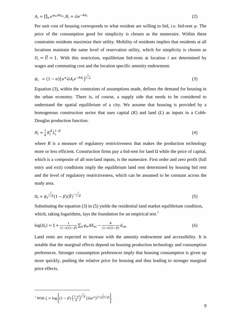
= ∏ , = (2)
Per unit cost of housing corresponds to what resident are willing to bid, i.e. bid-rent ψ. The
price of the consumption good for simplicity is chosen as the numeraire. Within these
constraints residents maximize their utility. Mobility of residents implies that residents at all
locations maintain the same level of reservation utility, which for simplicity is chosen as
= = 1. With this restriction, equilibrium bid-rents at location i are determined by
wages and commuting cost and the location specific amenity endowment.
= (1 − ) 1
1 (3)
Equation (3), within the constraints of assumptions made, defines the demand for housing in
the urban economy. There is, of course, a supply side that needs to be considered to
understand the spatial equilibrium of a city. We assume that housing is provided by a
homogenous construction sector that uses capital (K) and land (L) as inputs in a Cobb-
Douglas production function.
=1
1
(4)
where R is a measure of regulatory restrictiveness that makes the production technology
more or less efficient. Construction firms pay a bid-rent for land Ω while the price of capital,
which is a composite of all non-land inputs, is the numeraire. First order and zero profit (full
entry and exit) conditions imply the equilibrium land rent determined by housing bid rent
and the level of regulatory restrictiveness, which can be assumed to be constant across the
study area.
Ωi =
1
1(1 − )
1
1 (5)
Substituting the equation (3) in (5) yields the residential land market equilibrium condition,
which, taking logarithms, lays the foundation for an empirical test.1
logΩ = ξ +
∑ −
(6)
Land rents are expected to increase with the amenity endowment and accessibility. It is
notable that the marginal effects depend on housing production technology and consumption
preferences. Stronger consumption preferences imply that housing consumption is given up
more quickly, pushing the relative price for housing and thus leading to stronger marginal
price effects.
1 With ξ = log(1− ) 1
11 1
11.
10
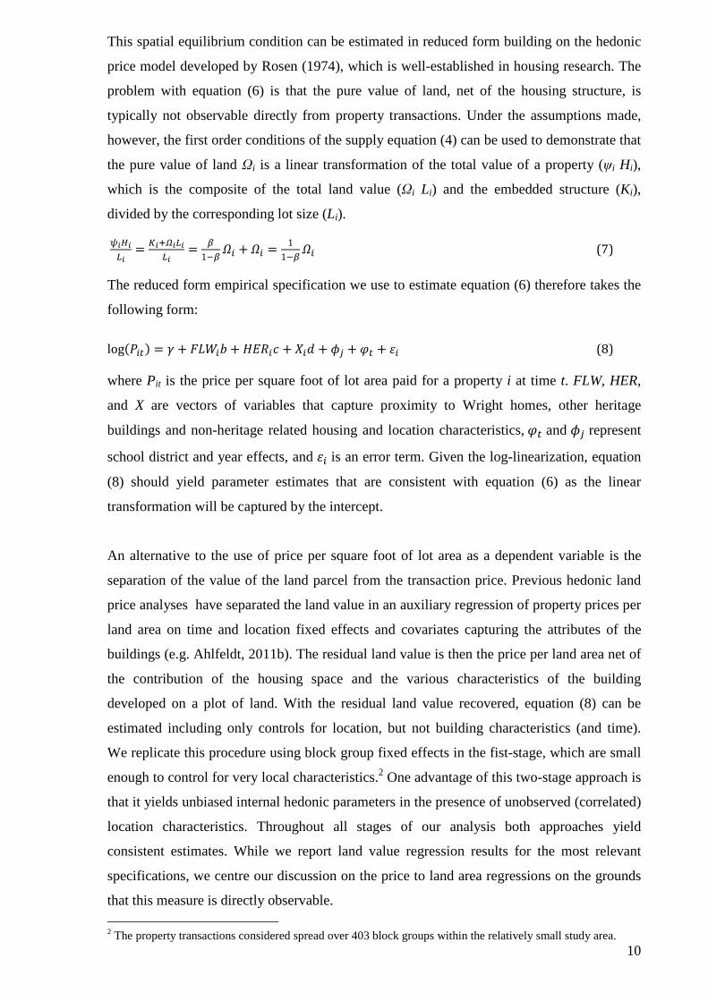
This spatial equilibrium condition can be estimated in reduced form building on the hedonic
price model developed by Rosen (1974), which is well-established in housing research. The
problem with equation (6) is that the pure value of land, net of the housing structure, is
typically not observable directly from property transactions. Under the assumptions made,
however, the first order conditions of the supply equation (4) can be used to demonstrate that
the pure value of land Ωi is a linear transformation of the total value of a property (ψi Hi),
which is the composite of the total land value (Ωi Li) and the embedded structure (Ki),
divided by the corresponding lot size (Li).
=
=
1 + =
1
1 (7)
The reduced form empirical specification we use to estimate equation (6) therefore takes the
following form:
log = + + + + ! + + " (8)
where Pit is the price per square foot of lot area paid for a property i at time t. FLW, HER,
and X are vectors of variables that capture proximity to Wright homes, other heritage
buildings and non-heritage related housing and location characteristics, and represent
school district and year effects, and is an error term. Given the log-linearization, equation
(8) should yield parameter estimates that are consistent with equation (6) as the linear
transformation will be captured by the intercept.
An alternative to the use of price per square foot of lot area as a dependent variable is the
separation of the value of the land parcel from the transaction price. Previous hedonic land
price analyses have separated the land value in an auxiliary regression of property prices per
land area on time and location fixed effects and covariates capturing the attributes of the
buildings (e.g. Ahlfeldt, 2011b). The residual land value is then the price per land area net of
the contribution of the housing space and the various characteristics of the building
developed on a plot of land. With the residual land value recovered, equation (8) can be
estimated including only controls for location, but not building characteristics (and time).
We replicate this procedure using block group fixed effects in the fist-stage, which are small
enough to control for very local characteristics.2 One advantage of this two-stage approach is
that it yields unbiased internal hedonic parameters in the presence of unobserved (correlated)
location characteristics. Throughout all stages of our analysis both approaches yield
consistent estimates. While we report land value regression results for the most relevant
specifications, we centre our discussion on the price to land area regressions on the grounds
that this measure is directly observable.
2 The property transactions considered spread over 403 block groups within the relatively small study area.
11
We note that the vector X does not include a control for housing size as building density is
endogenous in the model and incorporated into the spatial equilibrium condition (6) via the
supply side. Adding such a control to specification (8) presumably inflates the explanatory
power of the model at the risk of partially absorbing variation in prices that is originally
caused by the variables of interest (FWL), a so called bad control problem (Angrist &
Pischke, 2009). A similar argument applies to socio-economic composition of the
neighbourhood as some types of households may tend to locate closer to iconic architecture
because of particular preferences and tastes. In specification (8) school district fixed effects,
which we include to control for school quality and unobserved location effects, may also
capture socio-economic variation to some degree. School districts, however, are relatively
large so that we expect sufficient within school district variation to identify proximity to
Wright building effects. It is important to note, of course, that the location of Wright
buildings themselves could be endogenous, e.g. because they were built at the most suitable
locations. Failure to control for these conditions could yield biased estimates. We will
provide evidence, however, that controlling for historic conditions reflected in land values
does not affect the estimated proximity premium.
We prefer the transaction price per associated land unit (or the residual land value) to be the
dependent variable in a hedonic housing analysis since land within our study area is scarce
and the supply side can (largely) be ignored. With regard to (missing) controls for the size of
a property, this setup stands in some contrast to the common practice in the applied house
price capitalization literature, so we decided to run an alternative specification for selected
models with the (log) price of a property transaction as the dependent variable which
controls (including squares) for lot and floor size. Table 1 gives an overview on the control
variables used in this study.
The main (spatial) dimension of interest for this study is proximity to Frank Lloyd Wright
homes. Recent house price capitalization studies have used different spatial settings to
capture amenity effects. The most popular measure is distance from each observation to the
point of interest, with the results stating the (percentage) change in property prices with each
additional distance unit away. In many cases, the amenity such as a park or a lake has a use
to residents apart from visual impact and therefore the impact is felt over greater distances.
Some of the channels through which iconic architecture may capitalize into property prices
discussed in section 3 can have effects over larger distances if they are associated with a
benefit to a community as whole, e.g. tourist spending [1], image effects [2] or civic pride
[4]. To the contrary, the aesthetic utility [3] either associated with direct views out of a
12
window, from a garden or when passing by buildings regularly, canbe felt only over a
relatively short distance. Therefore, besides variables capturing distance to the nearest
Wright home, a set of dummy variables for properties within mutual exclusive distance rings
of 0-50 m, 50-100m, 100-250m, 250-500m, 500-1000m, and 1000m-2000m will be used to
allow for non-linearities in the distance effect.
With these distance variables the premium residents attach to having one Wright building in
close proximity can be measured (proximity effect). As demonstrated by Ahlfeldt & Maennig
(2010c) for listed historic buildings, there may be additional benefits of having a variety of
buildings of a particular style nearby as they jointly constitute a particular character of a
neighbourhood. A popular measure to capture the variety effect at the expense of ignoring
the proximity effect is a density variable that counts the number of buildings within a certain
distance or tract. We will use distance and density variables in conjunction to test whether,
conditional on having one Wright building in the neighbourhood (proximity effect), there is
an incremental benefit of having several Wright buildings nearby (variety effect). One
limitation of the density variable is that it restricts the impact of additional Wright buildings
to a certain area that has to be defined arbitrarily. Within this area, all Wright buildings are
treated in the same way, irrespectively of their distance to a given point of observation.
These limitations can be overcome with a potentiality measure that creates an index that
incorporates the distance to all Wright buildings (FLWPOT) and, hence, proximity and
variety effects simultaneously.
#$ = ∑ − (9)
, where τ determines that the spatial decay effect on average across all Wright buildings
diminishes with distance. It is estimated using a non-linear least squares estimator (NLS).
When used in conjunction with the distance variables mentioned above, a significant impact
of the latter will indicate that residents attach particular value to one Wright building in
proximity as opposed to proximity to several Wright buildings). Ahlfeldt and Maennig
(2010c) for historic landmarks in Berlin, which arguably exhibit a generally appealing but
not necessarily distinctive architecture, found a strong preference for variety but not for a
proximity effect . Given the uniqueness of the architectural style and the prestige attached to
a well known building and its architect, the proximity effect could be more important for
iconic landmarks.
6. Results We start the presentation of our results with the basic specifications, which focus on the
proximity effect discussed above. We assume that Wright buildings are perceived as perfect
13
substitutes and an associated location premium only depends on the proximity of a given
property to the nearest Wright building. Table 2 presents our findings. In models (1) and (2)
we regress the (log) transaction price per square foot of lot area on the distance to the nearest
Wright building and control for internal structural characteristics (except size), location
features and time of transaction. We find the (conditional) prices decline, on average, by
about 2.9% for each 1 km increase in straight line distance and 1.9% road distance to the
nearest Wright building. The difference in the coefficient estimates is perfectly in line with
road distances typically exceeding straight lines by about a factor of 1.5 (Ahlfeldt &
Maennig, 2009).3 These results are in line with the hypothesis of a significantly positive
amenity effect related to co-location with Wright buildings. While the effect may seem
quantitatively small in light of the limited variation in the distance (1km roughly corresponds
to a move from the lower to the upper quartile), it is still a (highly) statistically significant
impact.
As discussed above, the visual amenity of iconic residential architecture potentially exhibits
a very localized impact. Model (5) allows for a more flexible functional form by replacing
the continuous distance measure with dummy variables that denote selected distance bands.
The resulting pattern points to a significant premium of about 8.2% within 50m, diminishing
to about 6% in 50-100m and 5.2% in 100-250m, compared to a control group of properties
beyond 1km. Coefficients are not statistically significant for the 250-1000m area. This
pattern of results remains relatively stable when adding school district fixed effects and
controls for heritage builds, though the 0-50m dummy fails to satisfy conventional
significance criteria (4). It does also not change considerably when replacing the dependent
variable with residual land prices discussed in the context of the empirical strategy. For
further comparison we also replicate the full model with the log of sales price as dependent
variable, adding controls of lot size and floor size plus squares of both variables (6). Not
surprisingly in light of the bad control problem described in the section above, the
coefficients are slightly smaller in the model with potentially endogenous right hand side
controls (7% in the 0-50m and 3% in the 100-250m). A surprise, however, is that the 50-
100m area treatment coefficient becomes statistically insignificant. A closer look reveals that
building densities are significantly increased within this area.4 One admittedly ambitious
3 Road distances are calculated using MS Mappoint. 4 A regression of the floor-space-index (ratio of floor space over lot area) on the same explanatory variables as in model (4) indicates a significant differential within the 50-100m area (about 5%), but in none of the other distance rings.
14
interpretation could be that some buildings were built or extended to maximize the benefits
of the view despite properties not being located immediately adjacent to one another.5
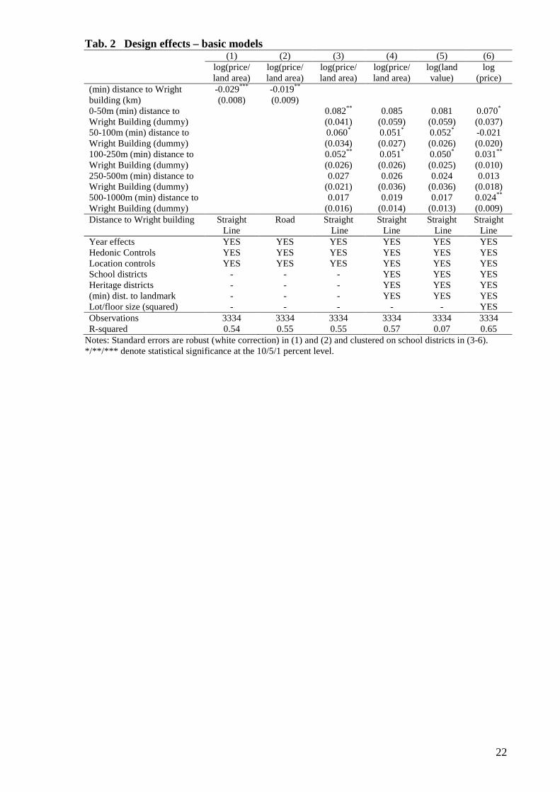
In the next step, we turn our attention to the variety effect discussed above, precisely on
whether, given the proximity effect found related to the nearest Wright building, there is any
incremental effect of having a larger number of Wright buildings nearby. In model (1) of
Table (3), we first add a variable that counts the number of Wright buildings within 250m
(Wright building density), a threshold based on the Table 2 estimates. We control for the
density of listed landmarks with a similarly defined variable (heritage density) to disentangle
the effects of Wright buildings and landmarks appropriately. The results for this specification
provide little support for the existence of a significant variety effect. The effect of the Wright
building density cannot be rejected from being zero. At the same time, the point estimates on
the effects of distance even slightly increase, even though significance levels are reduced.
To allow for a continuous effect of distance in the variety effect, we set up a potentiality
equation where each Wright building enters the equation with a weight depending on the
distance to a given property (see equation 9). We use a non-linear least squares estimator
(NLS) to estimate the spatial decay parameter τ. Note that in column (2) we omit other
heritage variables to not overload the NLS models. It turns out that the Wright potentiality
variable exhibits a positive and significant coefficient. In contrast to the level parameters,
however, the decay parameter is not estimated as satisfying statistical precision, which sheds
some doubts on the efficiency of the variable to capture the associated Wright building
amenity effects. At least, the estimated decay function is plausible as it indicates a localized
view effect largely concentrated in the first hundreds of meters around Wright buildings (see
Figure 2).
Holding the estimated decay parameters constant and adding heritage variables, including a
similarly defined heritage potentiality, as well as the distance to Wright building dummies
yields somewhat ambiguous results. On the one hand, the potentiality variable performs well
in the sense that it almost entirely picks up effects associated with distance to the nearest
Wright building, which is reflected in the distance dummy variable coefficients becoming
very close to and statistically undistinguishable from zero. On the other hand, the potentiality
variable itself fails to satisfy conventional significance criteria in this specification. This
pattern is indicative of a conflict between the distance dummy variable and the potentiality
5 Another explanation could be that the results are particularly sensitive to altering model specification because of too few observations in the distance band. However, with 84 and (2.5% of the all) observations in the 50-100m ring alone, the area seems reasonably populated.

15
variable in capturing a similar phenomenon. Given that the potentiality variable also covers
proximity to the nearest Wright building, the common theme emerging from a) significant
effects of nearest distance variables alone, b) insignificant effects of count variables (pure
measure of variety) and c) insignificant effects of potentiality variables when conditioning
on nearest building effects, suggests that the effects of iconic (Wright) architecture do not
operate primarily through a variety effect. Minimally, comparing these results to recent
findings in the historic preservation literature (Ahlfeldt & Maennig, 2010c; Lazrak, et al.,
2010; Noonan & Krupka, 2011), it seems fair to state that residents put a stronger emphasis
on having one iconic Wright building in their immediate proximity – presumably within
view distance of their property – than on proximity to an arbitrary historic building.
In the last step of the empirical analysis, we address the typical concern in cross-sectional
hedonic analyses that the estimated treatment effect could be the result of a spatial
correlation in the variable of interest and one or more unobserved location characteristics as
– no matter how sophisticated a model is – one can hardly control for all attributes that drive
the willingness to pay of the (marginal) buyers. In this specific case, such unobserved
location characteristics could have even determined the location of Wright buildings. In an
attempt to deal with this problem, we introduce a measure of the historic land value into our
specification. We argue that positive location features that were important enough to impact
the location of Wright buildings should have been capitalized in land values so that they can
be controlled for. One obvious way to respond to the problem, thus, would be to introduce a
measure of the value of location that dates back to a period before Wright buildings were
built, so to control for unobserved determinants of the location of Wright buildings without
confounding the measure with the effects of Wright buildings. To our knowledge, such a
measure that would predate the 1890s is not available at a sufficiently fine spatial level. The
earliest suitable data we could get hold of were assessed land values as provided in the 1913
edition of Olcott’s Land Value Blue Book of Chicago, which was just after all Wright
buildings considered in this analysis had been developed. Olcott’s land values enjoy a high
reputation in the academic literature and have been used in important contributions such as
McMillen (1996), although not at a similarly high spatial detail as we propose.6 A control for
1913 land valuation still adds important insights as it encompasses all relevant location
features of that time, including any potential external impact Wright buildings had right after
their construction. They allow, thus, for an investigation of whether the “iconic” view effect
of Wright buildings identified above is a relatively recent phenomenon, which we presume
6 Data from “Olcott’s Land Values Blue Book of Chicago” has also been used by Bednarz (1975), Berrry (1976), McDonald and Bowman (1979), McDonald (1981), McMillen (1979), McDonald and McMillan (1990), McMillen and McDonald (1991), Mills (1969), and Yates (1965).

16
given that the reputation of the architect clearly has increased with time and revolutionary
architecture may develop a wider appeal with a considerably delay due to slowly adjusting
preferences and tastes. If the Wright building premium was already fully priced in by 1913,
our extended specification, which effectively corresponds to a long difference in the
willingness to pay for land, should not reveal any additional effect of Wright building
proximity.
We make use of GIS to merge 1913 land values and contemporary transactions. First,
Olcott’s land value maps are georeferenced to fit with a geographic coordinate system
(decimal degrees). Second, each of the about 1200 land values provided on these maps for
the Oak Park study area is assigned to an individual (point) observation. Third, a spatial land
value surface is created using an inverse distance weight interpolation technique. Fourth,
interpolated land values are assigned to contemporary property transactions, which are
identified by geographic coordinates (latitudes / longitudes). The resulting spatial land value
surface is illustrated in Figure 3. To allow for a visual comparison, we also create a
contemporary land price surface. The contemporary land price proxy comes from a
regression of transaction prices per lot area on the hedonic controls listed in Table 1 plus
fixed effects for years and census block groups, which are then recovered and interpolated. A
correlation with the distribution of Wright buildings is evident from both maps, although
high land values are considerably more dispersed in the contemporary surface.
Columns (4-6) of Table 3 show the results for specifications that correspond to the respective
columns of Table 2, in each case extended by (log) of 1913 land values. It turns out that
neither in our preferred specification (4) nor in the alternative specifications (5-6) do historic
land values have a significant impact, conditional on the employed location controls.
Moreover, the estimated Wright building proximity effects remain virtually unchanged and
even slightly increase in (log) price regressions. These results indicate that the employed
location controls are strong and that, as suspected, the iconic design premium emerged over
time. It's noteworthy that in unpublished extended specifications we could not find evidence
for an increase in the proximity effect during our years of observation, indicating that the
adaption of preferences was completed before 2003.7 Finally we note that our results do not
seem to be sensitive to problems of spatial dependency. LM tests do not indicate the
presence of spatial specification problems and a robustness test with a spatial error correction
7 Our tests are based on an extended Table 2, column (1) specification introducing an interaction term of distance to the nearest Wright building and a yearly trend variable. We thank an anonymous referee for this suggestion.
17
model did not change the pattern of results qualitatively, but even slightly increased the point
estimates and the estimation precision.8
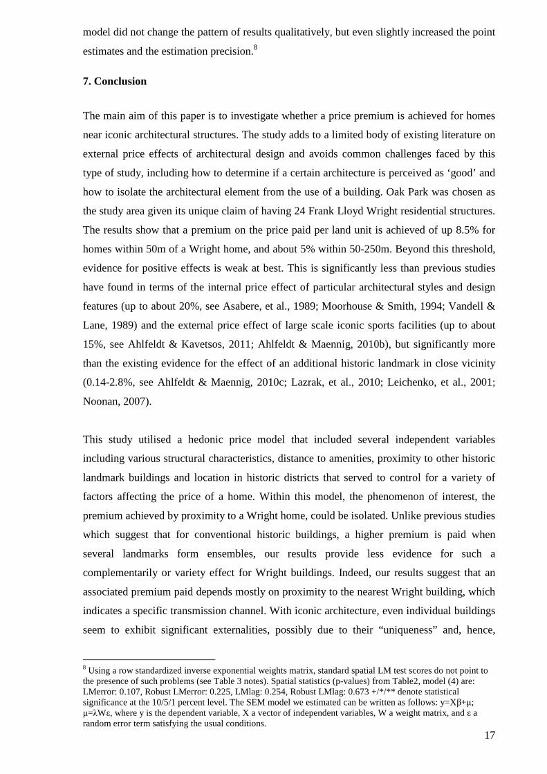
7. Conclusion
The main aim of this paper is to investigate whether a price premium is achieved for homes
near iconic architectural structures. The study adds to a limited body of existing literature on
external price effects of architectural design and avoids common challenges faced by this
type of study, including how to determine if a certain architecture is perceived as ‘good’ and
how to isolate the architectural element from the use of a building. Oak Park was chosen as
the study area given its unique claim of having 24 Frank Lloyd Wright residential structures.
The results show that a premium on the price paid per land unit is achieved of up 8.5% for
homes within 50m of a Wright home, and about 5% within 50-250m. Beyond this threshold,
evidence for positive effects is weak at best. This is significantly less than previous studies
have found in terms of the internal price effect of particular architectural styles and design
features (up to about 20%, see Asabere, et al., 1989; Moorhouse & Smith, 1994; Vandell &
Lane, 1989) and the external price effect of large scale iconic sports facilities (up to about
15%, see Ahlfeldt & Kavetsos, 2011; Ahlfeldt & Maennig, 2010b), but significantly more
than the existing evidence for the effect of an additional historic landmark in close vicinity
(0.14-2.8%, see Ahlfeldt & Maennig, 2010c; Lazrak, et al., 2010; Leichenko, et al., 2001;
Noonan, 2007).
This study utilised a hedonic price model that included several independent variables
including various structural characteristics, distance to amenities, proximity to other historic
landmark buildings and location in historic districts that served to control for a variety of
factors affecting the price of a home. Within this model, the phenomenon of interest, the
premium achieved by proximity to a Wright home, could be isolated. Unlike previous studies
which suggest that for conventional historic buildings, a higher premium is paid when
several landmarks form ensembles, our results provide less evidence for such a
complementarily or variety effect for Wright buildings. Indeed, our results suggest that an
associated premium paid depends mostly on proximity to the nearest Wright building, which
indicates a specific transmission channel. With iconic architecture, even individual buildings
seem to exhibit significant externalities, possibly due to their “uniqueness” and, hence,
8 Using a row standardized inverse exponential weights matrix, standard spatial LM test scores do not point to the presence of such problems (see Table 3 notes). Spatial statistics (p-values) from Table2, model (4) are: LMerror: 0.107, Robust LMerror: 0.225, LMlag: 0.254, Robust LMlag: 0.673 +/*/** denote statistical significance at the 10/5/1 percent level. The SEM model we estimated can be written as follows: y=Xβ+µ; µ=λWε, where y is the dependent variable, X a vector of independent variables, W a weight matrix, and ε a random error term satisfying the usual conditions.

18
higher associated visual utility and prestige. Notably, the iconic effect seems to have
emerged with delay as historic land values assessed right after the last Wright buildings had
been developed in the neighbourhood cannot account for the estimated contemporary
premium. This phenomenon may be related to an increase in prominence of the architect
over time or a relatively slow adaption of tastes and preferences to innovative architecture.
While the results from this study are interesting, they may not easily generalize to other
locations given the uniqueness of Frank Lloyd Wright’s architecture and popularity. In this
study, it is difficult to separate the prestige element from the actual architectural design and
it would be interesting to study the external impact of sophisticated design by lesser-known
architects. Still, the existence of significant externalities of iconic architecture opens avenues
for conceptionally appealing policies. One could argue that if better architecture were
achieved across the board, not only would liveable and enjoyable public spaces be created,
but, due to mutual externality effects, homeowners would also benefit from the increased
value of their neighbourhoods and eventually their properties. While in this scenario,
theoretically, everyone could be made better off, there is, of course, a downside to be
considered, requiring that the benefit of such policies be weighed carefully against the cost.
Enforcing higher investment into architecture, e.g. by imposing regulatory standards,
increases construction costs and potentially discourages (re)development. A rather
undesirable result would be a property price increase that is supply rather than demand
driven, with potentially negative welfare effects.9 Clearly, more research is required into the
nature of architectural externalities and associated welfare effects before fully informative
and reliable policy recommendations can be made.
9 In the model world, this scenario would correspond to an increase in R.

19
Figure 1: Frank Lloyd Wright Houses and Built Herit age in Oak Park, IL
Source: Own illustration. Background map from Google Maps.

20
Fig. 2 Spatial decay in Wright potentiality
Notes: Decay function based on Table 3, column (3) model estimate.. Fig. 3 Land Value and Land Price Prices 1913
2000s
Notes: Historic land values are estimates taken from the 1913 edition of Olcott’s Land Value Blue Book of Chicago. Current Land Prices are estimated in an auxiliary regression of residential transaction prices per square foot of land area on structural characteristics and census block group fixed effects, which are then retrieved. In both maps, for the purposes of visibility a continuous spatial surface is interpolated using an inverse distance weight interpolation technique.

21
Tab. 1 Control Variable Description Lot/floor size Size of lot in square ft Size of house in square ft Hedonic controls
A set of variables capturing the attributes below
Age in yrs of house Number of stories Number of bedrooms Number of bathrooms A (0,1) dummy variable equal to one if house is stand-alone single family A (0,1) dummy variable equal to one if building construction material is frame A (0,1) dummy variable equal to one if building construction material is masonry A (0,1) dummy variable equal to one if building construction material is masonry and
frame A (0,1) dummy variable equal to one if building construction material is stucco A (0,1) dummy variable equal to one if house’s basement is a formal recreational
room A (0,1) dummy variable equal to one if house’s basement is an apartment A (0,1) dummy variable equal to one if house’s basement is unfinished A (0,1) dummy variable equal to one if building has an attic A (0,1) dummy variable equal to one if house’s attic is an apartment A (0,1) dummy variable equal to one if house’s attic is unfinished A (0,1) dummy variable equal to one if house’s attic is a living area A (0,1) dummy variable equal to one if building has warm air heating A (0,1) dummy variable equal to one if building has hot water heating A (0,1) dummy variable equal to one if building has electric heating A (0,1) dummy variable equal to one if building has no heating A (0,1) dummy variable equal to one if building has air-conditioning Number of fireplaces Number of commercial units in building Number of car spaces in garage A (0,1) dummy variable equal to one if garage is attached to house A (0,1) dummy variable equal to one if garage is under the house A (0,1) dummy variable equal to one if house has porch A (0,1) dummy variable equal to one if house has been renovated Month (1-12) in which a transaction took place Historic Districts
A set of (0,1) dummy variables denoting following heritage districts: Frank Lloyd Wright-Prairie School of Architecture historic district, Ridgeland-Oak Park historic district and Gunderson historic district (see also Figure 1))
Location Controls
(Road) distance to the nearest highway entrance, (straight line) distance to the highway, distance to the town centre, distance to the nearest subway station, distance to the nearest park
School Districts A set of (0,1) dummy variables denoting following school districts (average test scores in parentheses): Mann (93.7), Lincoln (89.9), Longfellow (89.7), Beye (88.6), Holmes (87.3), Hatch (85.5), Irving (85.4), Whittier (82.3), Percy Julian (90.3), Gwendolyn Brooks (87.8)
Year Effects A set of (0,1) dummy variables each denoting a year 2003-2009
22
Tab. 2 Design effects – basic models (1) (2) (3) (4) (5) (6) log(price/
land area) log(price/ land area)
log(price/ land area)
log(price/ land area)
log(land value)
log (price)
(min) distance to Wright building (km)
-0.029*** (0.008)
-0.019** (0.009)
0-50m (min) distance to Wright Building (dummy)
0.082** (0.041)
0.085 (0.059)
0.081 (0.059)
0.070* (0.037)
50-100m (min) distance to Wright Building (dummy)
0.060* (0.034)
0.051* (0.027)
0.052* (0.026)
-0.021 (0.020)
100-250m (min) distance to Wright Building (dummy)
0.052** (0.026)
0.051* (0.026)
0.050* (0.025)
0.031** (0.010)
250-500m (min) distance to Wright Building (dummy)
0.027 (0.021)
0.026 (0.036)
0.024 (0.036)
0.013 (0.018)
500-1000m (min) distance to Wright Building (dummy)
0.017 (0.016)
0.019 (0.014)
0.017 (0.013)
0.024** (0.009)
Distance to Wright building Straight Line
Road Straight Line
Straight Line
Straight Line
Straight Line
Year effects YES YES YES YES YES YES Hedonic Controls YES YES YES YES YES YES Location controls YES YES YES YES YES YES School districts - - - YES YES YES Heritage districts - - - YES YES YES (min) dist. to landmark - - - YES YES YES Lot/floor size (squared) - - - - - YES Observations 3334 3334 3334 3334 3334 3334 R-squared 0.54 0.55 0.55 0.57 0.07 0.65
Notes: Standard errors are robust (white correction) in (1) and (2) and clustered on school districts in (3-6). */**/*** denote statistical significance at the 10/5/1 percent level.
23
Tab. 3 Design effects – extended models (1) (2) (3) (4) (5) (6) OLS NLS OLS OLS OLS OLS log(price/ land area)
log(price) log(price/ land area)
log(price/ land area)
log(land value)
log(price)
(min) distance to Wright 0.1 0.013 0.083 0.084 0.080* Building 0-50m (dummy) (0.08) (0.073) (0.056) (0.052) (0.033) (min) distance to Wright 0.08 -0.009 0.051* 0.053** -0.015 Building 50-100m (dummy) (0.048) (0.053) (0.022) (0.022) (0.018) (min) distance to Wright 0.062* 0.02 0.050* 0.051* 0.034** Building 100-250m (dummy) (0.03) (0.042) (0.024) (0.022) (0.01) (min) distance to Wright 0.024 0.008 0.023 0.026 0.018 Building 250-500m (dummy) (0.037) (0.061) (0.038) (0.034) (0.018) (min) distance to Wright 0.02 0.012 0.015 0.017 0.022* Building 500-1000m (dummy) (0.014) (0.02) (0.017) (0.013) (0.009) Wright building density -0.011 (Count within 250m) (0.007) Wright potentiality 0.007** 0.003 (FLWPOT) (0.002) (0.009) Decay parameter 1.646 (τ) (1.473) (log) Land value 1913 -0.002 -0.004 -0.018
(0.015) (0.014) (0.01) Year Effects YES YES YES YES - YES Hedonic controls YES YES YES YES - YES Location controls YES YES YES YES YES YES School Districts YES YES YES YES YES YES Heritage Density YES - - - - - Heritage District YES - YES YES YES YES (min) dist. to landmark YES - YES YES YES - Heritage potential - - YES - - YES Lot/floor size (squared) - - - - - YES Observations 3334 3334 3334 3334 3334 3334 R-squared 0.57 0.57 0.57 0.57 0.07 0.65
Notes: Heritage density and potentiality is defined analogically to Wright building density and Wright potentiality using all listed landmarks. Standard errors are clustered on school districts in all models. Standard errors in (2) are from OLS regressions holding the previously decay parameter estimated by means of NLS constant. */**/*** denote statistical significance at the 10/5/1 percent level.

24
References
Ahlfeldt, G. M. (2011). The Hidden Dimensions of Urbanity. Working Paper. Ahlfeldt, G. M., & Kavetsos, G. (2011). Form or Function? The impact of new football
stadia on property prices in London. SERC Discussion Paper 87. Ahlfeldt, G. M., & Maennig, W. (2009). Arenas, Arena Architecture and the Impact on
Location Desirability: The Case of “Olympic Arenas” in Berlin-Prenzlauer Berg. Urban Studies, 46(7), 1343-1362.
Ahlfeldt, G. M., & Maennig, W. (2010a). Impact of Sports Arenas on Land Values: Evidence from Berlin. The Annals of Regional Science, 44(2), 205-227.
Ahlfeldt, G. M., & Maennig, W. (2010b). Stadium Architecture and Urban Development from the Perspective of Urban Economics. International Journal of Urban and Regional Research, 34(3), 629-646.
Ahlfeldt, G. M., & Maennig, W. (2010c). Substitutability and Complementarity of Urban Amenities: External Effects of Built Heritage in Berlin. Real Estate Economics, 38(2), 285-323.
Anderson, S. T., & West, S. E. (2006). Open space, residential property values, and spatial context. Regional Science and Urban Economics, 36(6), 773-789.
Angrist, J. D., & Pischke, J.-S. (2009). Mostly Harmless Econometrics: An Empiricist's Companion: Princton University Press.
Asabere, P. K., Hachey, G., & Grubaugh, S. (1989). Architecture, Historic Zoning, and the Value of Homes. Journal of Real Estate Finance and Economics, 2(3), 181-195.
Bednarz, R. S. (1975). The Effect of Air Pollution on Property Value in Chicago. Chicago: University of Chicago Press.
Berry, B. J. L. (1976). Ghetto Expansion and Single-Family Housing Prices. Journal of Urban Economics, 3(4), 397.
Brewster, M. (Producer). (2004) Frank Lloyd Wright: America’s architect. Businessweek Online.
Coulson, N. E., & Lahr, M. L. (2005). Gracing the Land of Elvis and Beale Street: Historic Designation and Property Values in Memphis. Real Estate Economics, 33(3), 487-507.
Do, A. Q., & Grudnitski, G. (1995). Golf courses and residential house prices: An empirical examination. The Journal of Real Estate Finance and Economics, 10(3), 261-270.
Florida, R., Mellander, C., & Stolarick, K. (2009). Beautiful Places: The Role of Perceived Aesthetic Beauty in Community Satisfaction. Martin Prosperity Institute Working Paper.
Gat, D. (1998). Urban Focal Points and Design Quality Influence Rents: The Case of the Tel Aviv Office Market. Journal of Real Estate Research, 16(2), 229-247.
Gibbons, S., & Machin, S. (2008). Valuing school quality, better transport, and lower crime: evidence from house prices. Oxford Review of Economic Policy, 24(1), 99-119.
Glaeser, E. L., Kolko, J., & Saiz, A. (2001). Consumer city. Journal of Economic Geography, 1(1), 27-50.
Hough, D. E., & Kratz, C. G. (1983). Can "good" architecture meet the market test? Journal of Urban Economics, 14(1), 40-54.
Lazrak, F., Nijkamp, P., Rietveld, P., & Rouwendal, J. (2010). The market value of listed heritage: An urban economic application of spatial hedonic pricing. VU University Amsterdam Working Paper, http://www.tinbergen.nl/files/papers/flpnprjr_laatste_versie_okt_2010.pdf.
Leichenko, R. M., Coulson, N. E., & Listokin, D. (2001). Historic Preservation and Residential Property Values: An Analysis of Texas Cities. Urban Studies, 38(11), 1973-1987.
Mahan, B. L., Polasky, S., & Adams, R. M. (2000). Valuing Urban Wetlands: A Property Price Approach. Land Economics, 76(1), 100-113.
25
McDonald, J. F. (1981). Spatial patterns of business land values in chicago. Urban Geographie, 3, 201-215.
McDonald, J. F., & Bowman, H. W. (1979). Land value functions: A reevaluation. Journal of Urban Economics, 6(1), 25-41.
McDonald, J. F., & McMillen, D. P. (1990). Employment subcenters and land values in a polycentric urban area: the case of Chicago. Environment and Planning A, 22(5), 1561-1574.
McMillen, D. P. (1979). Economic analysis of an urban housing market. New York: Academic Press.
McMillen, D. P. (1996). One Hundred Fifty Years of Land Values in Chicago: A Nonparametric Approach. Journal of Urban Economics, 40(1), 100-124.
McMillen, D. P., & McDonald, J. F. (1991). Urban land value functions with endogenous zoning. Journal of Urban Economics, 29(1), 14-27.
Mills, E. S. (1969). The value of urban land. In H. Perloff (Ed.), The quality of urban environment. Baltimore, MA: Resources for the Future, Inc.
Mills, E. S. (1972). Studies in the Structure of the Urban Economy. Baltimore: Johns Hopkins Press.
Moorhouse, J. C., & Smith, M. S. (1994). The Market for Residential Architecture: 19th Century Row Houses in Boston's South End. Journal of Urban Economics, 35(3), 267-277.
Muth, R. F. (1969). Cities and Housing: The Spatial Pattern of Urban Residential Land Use. Chicago: University of Chicago Press.
Noonan, D. S. (2007). Finding an Impact of Preservation Policies: Price Effects of Historic Landmarks on Attached Homes in Chicago, 1990-1999. Economic development quarterly, 21(1), 17-33.
Noonan, D. S., & Krupka, D. J. (2011). Making—or Picking—Winners: Evidence of Internal and External Price Effects in Historic Preservation Policies. Real Estate Economics, 39(2), 379-407.
Rosen, S. (1974). Hedonic Prices and Implicit Markets: Product Differentiation in Pure Competition. Journal of Political Economy, 82(1), 34-55.
Song, Y., & Knaap, G.-J. (2003). New urbanism and housing values: a disaggregate assessment. Journal of Urban Economics, 54(2), 218-238.
Sprague, P. E. (1986). Guide to Frank Lloyd Wright & Prairie School Architecture in Oak Park: USA: Village of Oak Park.
Vandell, K. D., & Lane, J. S. (1989). The Economics of Architecture and Urban Design: Some Preliminary Findings. Journal of the American Real Estate & Urban Economics Association, 17(2), 235-260.
Village of Oak Park Community Planning and Development. (2010a). Frank Lloyd Wright-Prairie School of Architecture Brochure. http://www.oak-park.us/Planning/Historic_Preservation.html, Retrieved on July 6, 2010.
Village of Oak Park Community Planning and Development. (2010b). Gunderson Historic District Brochure. Http://www.oak-park.us/Planning/Historic_Preservation.html, Retrieved on July 6, 2010.
Village of Oak Park Community Planning and Development. (2010c). Ridgeland-Oak Park Historic District Brochure. http://www.oak-park.us/Planning/Historic_Preservation.html, Retrieved on July 6, 2010.
Wu, J., Adams, R. M., & Plantinga, A. J. (2004). Amenities in an Urban Equilibrium Model: Residential Development in Portland, Oregon. Land Economics, 80(1), 19-32.
Yeates, M. H. (1965). Some Factors Affecting the Spatial Distribution of Chicago Land Values, 1910-1960. Economic Geography, 41(1), 57-70.
Related Documents