The Trade-FDI Nexus: Evidence from the European Union Valeriano Martínez-San Román Marta Bengoa-Calvo Blanca Sánchez-Robles Rute 2013 / 15

Welcome message from author
This document is posted to help you gain knowledge. Please leave a comment to let me know what you think about it! Share it to your friends and learn new things together.
Transcript

The Trade-FDI Nexus: Evidence from the European Union
Valeriano Martínez-San Román Marta Bengoa-Calvo Blanca Sánchez-Robles Rute
2013 / 15
The Trade-FDI Nexus: Evidence from the European Union
Valeriano Martínez-San Román
Universidad de Cantabria
Marta Bengoa-Calvo
City College of New York (CUNY)
Colin Powell Center for Policy Studies
2013 / 15
Abstract
The objective of this paper is to examine the relationship between international
trade and Foreign Direct Investment (FDI) empirically. It analyses whether the
reduction of trade barriers over time has increased FDI for the particular case of
the European Union (EU) during the period from 1995 to 2009. To analyze this
issue the authors estimate in first place the European Border Effect by means of a
gravity equation. Once the border effect is obtained we test whether there is a
positive (complementary) or negative (substitution) relationship between this
border effect and the FDI within the European countries. A gravity model for
trade and FDI is estimated using the Poisson pseudo-maximum likelihood. The
results suggest that there is a positive and decreasing border effect up to 2007
while it turns upward for 2008 and 2009, offsetting the previous decline. For the
particular case of the EU, commercial integration and FDI reinforce each other,
thus being complements rather than substitutes. In addition to trade integration
measures, this paper also analyzes the potential role of other traditional
determinants of FDI, as the market size of the host country and the cost
differential among home-host economies. Cost differentials are not as relevant as
the possibility of gaining market share which leads us to conclude that in the EU
the FDI pattern follows a market-seeking strategy rather than a cost-efficient
model.
Keywords: International Trade; FDI; Gravity model; Home Bias; Border Effect;
European Union
JEL classification: F10; F14; F15, F21
Blanca Sánchez-Robles Rute
Universidad de Cantabria
1
The Trade-FDI Nexus: Evidence from the European Union
Valeriano Martínez San Román Universidad de Cantabria
Marta Bengoa Calvo City College of New York (CUNY)
Colin Powell Center for Policy Studies [email protected]
Blanca Sánchez-Robles Rute
Universidad de Cantabria [email protected]
ABSTRACT The objective of this paper is to examine the relationship between international trade and Foreign Direct Investment (FDI) empirically. It analyses whether the reduction of trade barriers over time has increased FDI for the particular case of the European Union (EU) during the period from 1995 to 2009. To analyze this issue the authors estimate in first place the European Border Effect by means of a gravity equation. Once the border effect is obtained we test whether there is a positive (complementary) or negative (substitution) relationship between this border effect and the FDI within the European countries. A gravity model for trade and FDI is estimated using the Poisson pseudo-maximum likelihood. The results suggest that there is a positive and decreasing border effect up to 2007 while it turns upward for 2008 and 2009, offsetting the previous decline. For the particular case of the EU, commercial integration and FDI reinforce each other, thus being complements rather than substitutes. In addition to trade integration measures, this paper also analyzes the potential role of other traditional determinants of FDI, as the market size of the host country and the cost differential among home-host economies. Cost differentials are not as relevant as the possibility of gaining market share which leads us to conclude that in the EU the FDI pattern follows a market-seeking strategy rather than a cost-efficient model. Keywords: International Trade; FDI; Gravity model; Home Bias; Border Effect; European Union JEL classification: F10; F14; F15, F21.
2
1. INTRODUCTION
The opening decade of the 21st century has witnessed a remarkable increase of
flows between countries, both in terms of trade and of investment. A favourable
economic climate during the first part of the decade and a widespread trend among
firms towards the geographical reorganization of production have been some of the
reasons underlying this pattern.
Not surprisingly, the global stock of inward Foreign Direct Investment (FDI
mounted from US$ 7.5 trillion in 2000 to US$ 19 trillion in 2010, its share in world
GDP rising from 23% in 2000 to over 31% in 2010. In turn, trade in goods and
services has grown from US$ 16 trillion in 2000 to over US$ 37 trillion in 2010. The
ratio world trade to GDP has increased 10 percentage points (from 49% in 2000 to
59%) during the first decade of the 21st century (UNCTAD, 2010a, 2011a).
The financial and economic crisis of the second half of the decade, however, has
induced a turning point in the upward trend of trade and FDI. Thus, inward FDI flows
fell 15% in 2008, 37% in 2009 and increased only by a modest 5% in 2010. The total
amount of FDI inflows was 37% lower in 2010 than in 2007. (UNCTAD, 2010b,
2011b)
Trade has also decreased during the economic crisis. After a significant
slowdown in 2008, the volume of world trade dropped by over 13% in 2009, this fall
representing its greatest decline since World War II. However, the volume of world
merchandise trade registered a 14 per cent increase in 2010, which roughly offset its
decline in 2009.
The expansion in international trading and investment activities has coincided
over time with an increase in the number of Regional Economic Integration
Agreements (RIAs) and with a further deepening in the removal of restrictions on
3
factor movements. For the particular case of the European Union –and in addition to
the 1992 Single European Act, which fully liberalized the internal mobility of goods,
services, capital and people, and an extension in 1995– other important landmarks
in the 21st century have been the implementation of the single currency in 2002 and
subsequent enlargements in 2004 and 2007.
This paper focuses on two particular aspects of the integration process of the
European economy. First, it analyses to what extent the institutional steps mentioned
above correspond in effect to a more integrated over time EU, as far as trade is
concerned. For this purpose the paper proposes and estimates an indicator of trade
integration, the so-called border effect or home bias. Second, it assesses the
connection between trade integration and FDI flows within the EU. The home bias is
the effect whereby consumers prefer domestic to foreign goods of similar
characteristics. Its presence in even highly integrated areas has been regarded as
one of the six major puzzles in international economics (Obstfeld and Rogoff, 2001).
The path breaking contribution of Mccallum (1995), which used a gravity model as
his framework of analysis and found a substantial degree of home bias in the
Canadian-USA trade, was followed by other pieces of research covering OCDE
countries (Wei, 1996, 1998), the EU (Nitsch, 2000; Chen, 2004; Quian, 2007) and the
border effect between the regions that encompass specific countries (Combes et al.,
2005; Gil Pareja et al., 2005; Wolf, 2009; Llano et al., 20011; Esteban et al., 2012.
The size of the home bias, as documented by these and other papers, is still a
matter of controversy, and according to some authors (Helliwell, 1998; Anderson and
Wincoop, 2003; Liu et al., 2010) it is heavily contingent upon the methodology
employed for its estimation and the variables included. Wei (1996, 1998) found a
4
home bias of 10 for the OCDE countries whereas Nitsch reported a value of 11.3 for
EU countries.
Econometric analyses of this issue have become more sophisticated over time.
Santos-Silva and Tenreyro (2006) have replaced the original log linear estimations of
the gravity model by an equation in multiplicative form and propose Poisson Pseudo-
Maximum Likelihood estimation (PPML). This approached has also been used by
Llano et al (2011), while Dias (2010, 2011) employs a non linear specification.
The literature has not reached a consensus yet on the sign of the connection
between trade and FDI. On a priori grounds, it is reasonable to assert that trade and
FDI are alternative ways of serving a foreign market, thus the correlation being
negative. As a matter of fact, some early empirical studies highlighted the existence
of a substitution relationship between trade and FDI (Mundell, 1957, Graham, 1996;
Bayoumi and Lipworth, 1997; Nakamura and Oyama, 1998). Contrarily to this view,
though, other contributions argue that FDI and trade are complements rather than
substitutes (Pfaffermayer, 1996; Brainard, 1997; Brenton et al, 1999;
Balasubramanyam et al, 2002, Egger and Pfaffermayer, 2004a, 2004b; Cuadros et
al, 2004; Alguacil et al, 2008; Neary, 2009; Martinez et al, 2012a). Furthermore,
another group o papers has found both types of relationship, of complementarity and
of substitution, between trade and FDI (Goldberg and Klein, 1999; Blonigen, 2001,
Head and Ries, 2001, Swenson, 2004; Fillat-Castejón et al, 2008). These authors
find that trade and FDI are complements in aggregate terms whereas depending on
the industry analysed, they can behave either as substitutes or complements.
The remainder of the paper is as follows. Section 2 presents a discussion of our
conceptual framework along with a brief summary of the data and the empirical
5
specifications considered in this paper. We report our findings in the third section and
conclude with policy implications and possible extensions.
2. EMPIRICS
2.1. GRAVITY MODEL
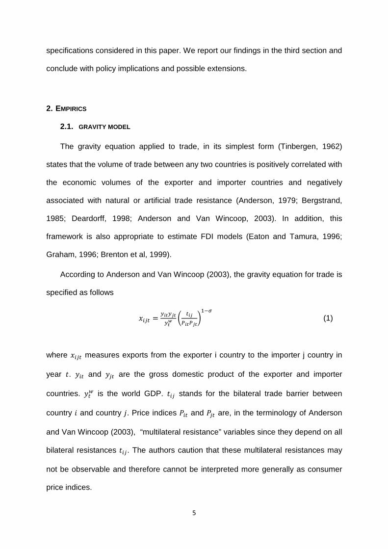
The gravity equation applied to trade, in its simplest form (Tinbergen, 1962)
states that the volume of trade between any two countries is positively correlated with
the economic volumes of the exporter and importer countries and negatively
associated with natural or artificial trade resistance (Anderson, 1979; Bergstrand,
1985; Deardorff, 1998; Anderson and Van Wincoop, 2003). In addition, this
framework is also appropriate to estimate FDI models (Eaton and Tamura, 1996;
Graham, 1996; Brenton et al, 1999).
According to Anderson and Van Wincoop (2003), the gravity equation for trade is
specified as follows
���� = �������
� �������
��� (1)
where ���� measures exports from the exporter i country to the importer j country in
year �. ��� and ��� are the gross domestic product of the exporter and importer
countries. ��� is the world GDP. ��� stands for the bilateral trade barrier between
country � and country �. Price indices ��� and ��� are, in the terminology of Anderson
and Van Wincoop (2003), “multilateral resistance” variables since they depend on all
bilateral resistances ���. The authors caution that these multilateral resistances may
not be observable and therefore cannot be interpreted more generally as consumer
price indices.
6
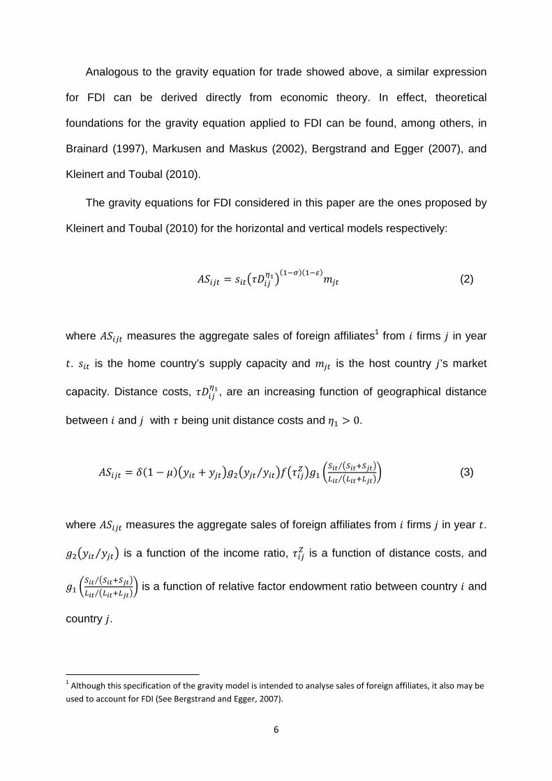
Analogous to the gravity equation for trade showed above, a similar expression
for FDI can be derived directly from economic theory. In effect, theoretical
foundations for the gravity equation applied to FDI can be found, among others, in
Brainard (1997), Markusen and Maskus (2002), Bergstrand and Egger (2007), and
Kleinert and Toubal (2010).
The gravity equations for FDI considered in this paper are the ones proposed by
Kleinert and Toubal (2010) for the horizontal and vertical models respectively:
����� = ����������� ���! ��"!#�� (2)
where ����� measures the aggregate sales of foreign affiliates1 from � firms � in year
�. ��� is the home country’s supply capacity and #�� is the host country �’s market
capacity. Distance costs, ������, are an increasing function of geographical distance
between � and � with � being unit distance costs and $� > 0.
����� = ' 1 − *!���� + ����,-���� ���⁄ �/����0�,� �1�� �1��21��⁄3�� �3��23��⁄ (3)
where ����� measures the aggregate sales of foreign affiliates from � firms � in year �. ,-���� ���⁄ � is a function of the income ratio, ���0 is a function of distance costs, and
,� �1�� �1��21��⁄3�� �3��23��⁄ is a function of relative factor endowment ratio between country � and
country �.
1 Although this specification of the gravity model is intended to analyse sales of foreign affiliates, it also may be
used to account for FDI (See Bergstrand and Egger, 2007).
7
2.2. DATA
The OECD in their Structural Analysis Dataset (STAN) and International Direct
Investment database provides data on bilateral exports and bilateral foreign direct
investment, respectively. Disaggregated bilateral exports data is measured in current
US dollars for each of the 23 industries considered while FDI data is provided on
aggregate bases and also measured in current US dollars. The GDPs in real terms
and US dollars are taken from the National Accounts Dataset provided by the OECD.
Bilateral trade flows and FDI series have been deflated using the GDPs deflactors
taken from the National Accounts Dataset as well.
In order to account for the “countries’ imports from themselves” data, which are
necessary to estimate the home bias effect, we have followed Wei (1996) computing
this variable for each industry and country as the difference between total production
of goods and exports to the rest of the world. Data on these variables have been also
extracted from the STAN Datasets and deflated using GDPs deflactors.
Data provided by the Centre d´Etudes Prospectives et d´Informations
Internationals (CEPII) is used to account for bilateral and intra-national distances and
also to account for adjacency and language dummies. Bilateral geodesic distances
are calculated following the great circle formula, which uses latitudes and longitudes
of the most important cities/agglomerations (in terms of population) in each country.
The internal distance of a country, which is a proxy of the average distance between
producer and consumers in a country is calculated using the area-based formula
proposed by Head and Mayer (2002)2. Language variable takes value 1 if two
2 ��� = 0.67789:;<
8
countries share the same official language, adjacency variable measure whether two
countries are contiguous –share land border–.
Relative factor endowments, needed to estimate the FDI models, have been
constructed using data on skilled3 and total employment from the Yearbook of Labour
Statistics published by the international labour organization (ILO).
Other variables such as the Corruption Perception Index or Trade Freedom
Indices are provided by Transparency International and The Heritage Foundation
respectively.
2.3. EMPIRICAL FRAMEWORK
In the first part of this section, to estimate the border effect by means of a gravity
equation, data on bilateral trade for 23 sectors of activity among 19 European
countries4 over the period 1995 to 2009 has been used. We follow Gourieroux, et al.
(1984a, 1984b) and Santos-Silva and Tenreyro (2006) to estimate a Poisson
Pseudo-Maximum Likelihood model (PPML). This estimation technique is robust to
different patterns of heteroskedasticity and provides a natural way to deal with zeros
in our data5.
The standard log-linear specification of the gravity model has important
disadvantages over a non-linear specification. Santos-Silva and Tenreyro (2006)
show that in the presence of heteroskedasticity in the error term, the parameters of
3 Skilled employment is defined as the sum of occupational categories 1 (legislators, senior officials and managers), 2 (professionals) and 3 (technicians and associate professionals) from the ISCO-88 classification.
4 Austria, Belgium, Czech Republic, Denmark, Finland, France, Germany, Greece, Hungary, Ireland, Italy, Netherlands, Belgium-Luxembourg (considered jointly), Poland, Portugal, Spain, Slovakia, Sweden and the United Kingdom.
5 Panel dataset has 111,780 observations (23-sectors x 18-exporting countries x 18-importing countries x 15-years) of which 4,463 are zero.
9
log-linearized models estimated by OLS lead to biased estimations of the true
elasticities since the log-linearization of the dependent variable changes the
properties of the error term, which becomes correlated with the explanatory variables
in the presence of heteroskedasticity (the Jensen’s inequality). In addition, log-
linearization is not compatible with the presence of zero values in the dependent
variable. Empirically, the PPML method estimates the parameters by entering the
dependent variable in levels while the independent ones are expressed in natural
logarithms.
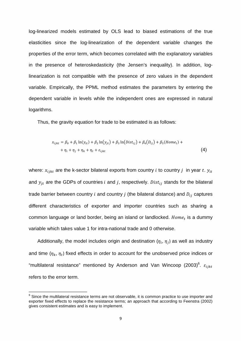
Thus, the gravity equation for trade to be estimated is as follows:
���=� = >? + >� ln ���! + >- ln����� + >B ln�������� + >C����� + >D EF#G�! +
+$� + $� + $= + $� + I��=� (4)
where: ���=� are the k-sector bilateral exports from country � to country � in year �. ���
and ��� are the GDPs of countries� and �, respectively. ������ stands for the bilateral
trade barrier between country � and country � (the bilateral distance) and ��� captures
different characteristics of exporter and importer countries such as sharing a
common language or land border, being an island or landlocked. EF#G� is a dummy
variable which takes value 1 for intra-national trade and 0 otherwise.
Additionally, the model includes origin and destination ($�, $�) as well as industry
and time ($=, $�) fixed effects in order to account for the unobserved price indices or
“multilateral resistance” mentioned by Anderson and Van Wincoop (2003)6. I��=� refers to the error term.
6 Since the multilateral resistance terms are not observable, it is common practice to use importer and exporter fixed effects to replace the resistance terms; an approach that according to Feenstra (2002) gives consistent estimates and is easy to implement.
10
On an a priori basis, bilateral exports from country � to country � are supposed to
show a positive relation with the economic sizes of both countries; as well as sharing
special characteristics such as language or a common land border are supposed to
reduce transaction costs and consequently foster bilateral trade. The bilateral
distance between them should act as a barrier to trade so it should exhibit a negative
sign.
For the purpose of this paper, the key parameters in equation (4) are those
corresponding to the dummy for EF#G� since we can recover yearly border effects
from their point estimates. The exponential of the coefficient of EF#G�, is the ratio of
intra-national trade to international trade for certain year, country or industry, after
controlling for size of GDP, distance, language, adjacency…7 Therefore, small
estimates for the home dummies indicate a lower relative weight of intra-national
trade and thus an increase in the importance of international trade in the countries,
industries or years of the sample, i.e., greater trade integration.
The next step is to test whether trade integration, measured as the inverse of the
evolution of home bias, is correlated with FDI. In order to do so, we construct a trade
integration variable based on the previously estimates of home bias. Firstly we
normalize the home bias estimates (equalizing 1995’s to one). The reason for doing
this is to eliminate the size of the estimates since it depends crucially on the measure
of intra-national distances used in the estimation (see Wei (1996) for a very good
example). Once we have normalized the coefficients, we calculate their inverse to
obtain our measure of trade integration (JK�G,LM!.
7 See, among others, McCallum (1995), Helliwell (1996), Wei (1996), Nitsch (2000), Wolf (2009), Chen (2004)
and Liu et al. (2010) for further explanation.
11
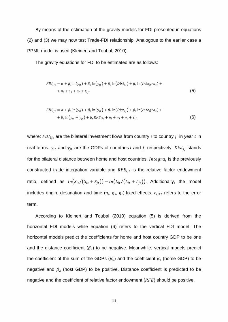
By means of the estimation of the gravity models for FDI presented in equations
(2) and (3) we may now test Trade-FDI relationship. Analogous to the earlier case a
PPML model is used (Kleinert and Toubal, 2010).
The gravity equations for FDI to be estimated are as follows:
N�J��� = O + >� ln ���! + >- ln����� + >B ln�������� + >C ln JK�G,LM�! +
+$� + $� + $� + I��� (5)
N�J��� = O + >� ln ���! + >- ln����� + >B ln�������� + >C ln JK�G,LM�! +
+>D ln���� + ���� + >PQNR��� + $� + $� + $� + I��� (6)
where: N�J��� are the bilateral investment flows from country � to country � in year � in
real terms. ��� and ��� are the GDPs of countries� and �, respectively. ������ stands
for the bilateral distance between home and host countries. JK�G,LM� is the previously
constructed trade integration variable and QNR��� is the relative factor endowment
ratio, defined as SK���� ���� + ����⁄ � − SK�T�� �T�� + T���⁄ �. Additionally, the model
includes origin, destination and time ($�, $�, $�) fixed effects. I��=� refers to the error
term.
According to Kleinert and Toubal (2010) equation (5) is derived from the
horizontal FDI models while equation (6) refers to the vertical FDI model. The
horizontal models predict the coefficients for home and host country GDP to be one
and the distance coefficient (>B) to be negative. Meanwhile, vertical models predict
the coefficient of the sum of the GDPs (>D) and the coefficient >� (home GDP) to be
negative and >- (host GDP) to be positive. Distance coefficient is predicted to be
negative and the coefficient of relative factor endowment (QNR) should be positive.
12
3. RESULTS
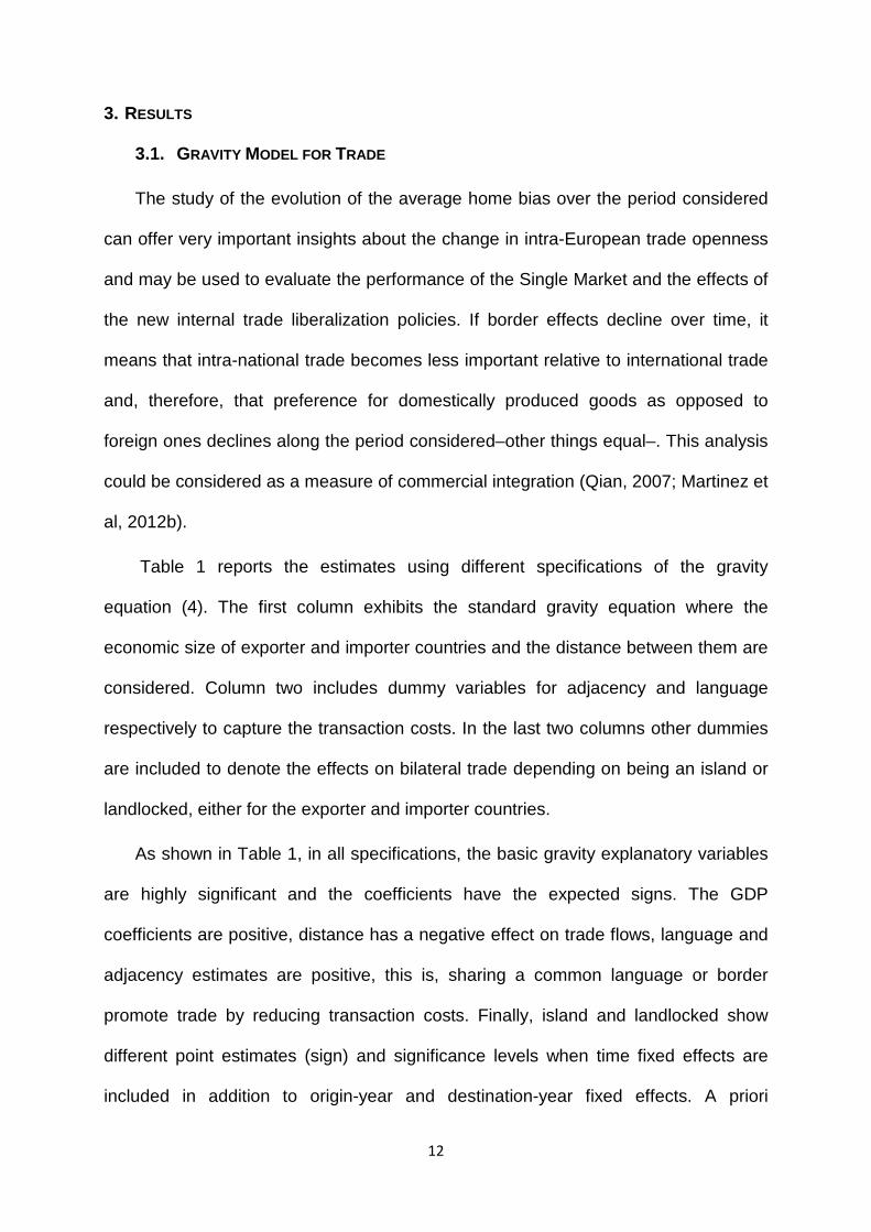
3.1. GRAVITY MODEL FOR TRADE
The study of the evolution of the average home bias over the period considered
can offer very important insights about the change in intra-European trade openness
and may be used to evaluate the performance of the Single Market and the effects of
the new internal trade liberalization policies. If border effects decline over time, it
means that intra-national trade becomes less important relative to international trade
and, therefore, that preference for domestically produced goods as opposed to
foreign ones declines along the period considered–other things equal–. This analysis
could be considered as a measure of commercial integration (Qian, 2007; Martinez et
al, 2012b).
Table 1 reports the estimates using different specifications of the gravity
equation (4). The first column exhibits the standard gravity equation where the
economic size of exporter and importer countries and the distance between them are
considered. Column two includes dummy variables for adjacency and language
respectively to capture the transaction costs. In the last two columns other dummies
are included to denote the effects on bilateral trade depending on being an island or
landlocked, either for the exporter and importer countries.
As shown in Table 1, in all specifications, the basic gravity explanatory variables
are highly significant and the coefficients have the expected signs. The GDP
coefficients are positive, distance has a negative effect on trade flows, language and
adjacency estimates are positive, this is, sharing a common language or border
promote trade by reducing transaction costs. Finally, island and landlocked show
different point estimates (sign) and significance levels when time fixed effects are
included in addition to origin-year and destination-year fixed effects. A priori
13
expectations for these coefficients are not straightforward; on the one hand, being an
island or landlocked reduce potential exports due to transport limitations. On the
other hand, they may raise bilateral exports due to the increase in the multilateral
resistances. Results obtained are not conclusive in this regards since coefficients
vary in sign and significance across specifications. These changes may be due to the
fact that only 2 countries out of 19 (Ireland and the United Kingdom) are islands and
solely 4 out of 19 are landlocked (Austria, Czech Rep., Hungary and Slovakia).
Moreover, except for the United Kingdom, their economic size and their relative
commercial proportion are small.
In order to retrieve the border effect from the estimations we should calculate the
exponential of the point estimate of the EF#G variable. That is, taking forth column
and year 2009 (EF#G-??U = 2.689), on average, a European country traded 14.7
times (exp^ 2.689!= 14.71) more with itself than with another European partner.
According to the estimations presented in table 1, the average overall border
effect shows a net increase of around 3% from 1995 to 2009 for the EU-19 countries
(see table 2). Point estimates for the border effects in column 1 show lower values
than in the rest of columns; however, since this is a very basic model where some
relevant variables are omitted, those coefficients may be biased. Once dummy
variables are included, and different fixed effects are considered, the border effects
rise but show comparable values across specifications.
14
TABLE 1. GRAVITY EQUATION FOR TRADE WITH YEARLY BORDER EFFECTS.
VARIABLES (1) (2) (3) (4)
Ln (Yi) 1.000 ** (0.064) 1.049 ** (0.082) 1.203 ** (0.070) 1.201 ** (0.064)
Ln (Yj) 1.099 ** (0.061) 1.156 ** (0.072) 1.284 ** (0.075) 1.144 ** (0.083)
Ln (Distij) -1.389 ** (0.017) -0.941 ** (0.021) -0.9360 ** (0.021) -0.971 ** (0.022)
Adjacency 0.554 ** (0.033) 0.596 ** (0.032) 0.594 ** (0.034)
Common Language 1.031 ** (0.039) 1.018 ** (0.039) 1.040 ** (0.040)
Islandi 1.779 ** (0.212) -1.349 ** (0.168)
Islandj -2.597 ** (0.288) -0.530 * (0.239)
Landlockedi 2.598 ** (0.174) 0.476 * (0.191)
Landlockedj -2.340 ** (0.269) -2.966 ** (0.311)
Home 1995 1.720 ** (0.064) 2.623 ** (0.071) 2.626 ** (0.071) 2.667 ** (0.093)
Home 1996 1.864 ** (0.058) 2.776 ** (0.066) 2.741 ** (0.066) 2.757 ** (0.068)
Home 1997 1.947 ** (0.058) 2.858 ** (0.066) 2.818 ** (0.066) 2.835 ** (0.068)
Home 1998 1.941 ** (0.060) 2.848 ** (0.067) 2.811 ** (0.067) 2.825 ** (0.069)
Home 1999 1.973 ** (0.060) 2.878 ** (0.067) 2.844 ** (0.067) 2.862 ** (0.069)
Home 2000 2.053 ** (0.060) 2.959 ** (0.067) 2.916 ** (0.067) 2.935 ** (0.069)
Home 2001 2.079 ** (0.062) 2.979 ** (0.069) 2.975 ** (0.069) 2.997 ** (0.071)
Home 2002 2.043 ** (0.062) 2.951 ** (0.069) 2.909 ** (0.069) 2.928 ** (0.070)
Home 2003 1.879 ** (0.061) 2.786 ** (0.068) 2.743 ** (0.068) 2.760 ** (0.070)
Home 2004 1.766 ** (0.063) 2.671 ** (0.069) 2.631 ** (0.069) 2.654 ** (0.071)
Home 2005 1.719 ** (0.063) 2.631 ** (0.069) 2.588 ** (0.069) 2.602 ** (0.071)
Home 2006 1.667 ** (0.064) 2.580 ** (0.071) 2.539 ** (0.070) 2.554 ** (0.072)
Home 2007 1.592 ** (0.064) 2.484 ** (0.071) 2.474 ** (0.070) 2.479 ** (0.072)
Home 2008 1.627 ** (0.078) 2.510 ** (0.083) 2.503 ** (0.082) 2.508 ** (0.084)
Home 2009 1.758 ** (0.080) 2.649 ** (0.083) 2.664 ** (0.082) 2.689 ** (0.084)
# Observations 109,932 109,953 109,881 109,400
R2 0.881 0.882 0.883 0.882
Source: Own elaboration.
Notes: Poisson pseudo-maximum likelihood estimation. The dependent variable is the real bilateral exports from country i to country j. Clustered robust standard errors in parentheses. *, ** denote significant at the 5% and 1% level, respectively. Industry fixed effects and year-specific exporter and importer fixed effects are included in all the regressions (Feenstra, 2002). The last column also includes time fixed effects.
In all the specifications a very similar pattern arises for the border effect
estimates and three stages may be easily identified. In a first stage they show
increasingly higher values until 2001. A second period, from 2002 to 2007 is
characterised by a sharp decline in border effects. Finally, the border effect increases
15
again in the last two years of analysis. Up to 2001, border effects increase by around
40 per cent in the EU; while there seems to be a commercial integration for the
period from 2001 to 2007, when the decline averages, again, the 40%. The increase
in the last two years goes from 18 to 23 per cent, being especially important in 2009
when the border effect increased by 14 to 19 per cent from the previous year
depending on the specification considered.
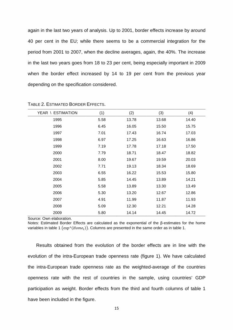
TABLE 2. ESTIMATED BORDER EFFECTS.
YEAR \ ESTIMATION (1) (2) (3) (4)
1995 5.58 13.78 13.68 14.40
1996 6.45 16.05 15.50 15.75
1997 7.01 17.43 16.74 17.03
1998 6.97 17.25 16.63 16.86
1999 7.19 17.78 17.18 17.50
2000 7.79 18.71 18.47 18.82
2001 8.00 19.67 19.59 20.03
2002 7.71 19.13 18.34 18.69
2003 6.55 16.22 15.53 15.80
2004 5.85 14.45 13.89 14.21
2005 5.58 13.89 13.30 13.49
2006 5.30 13.20 12.67 12.86
2007 4.91 11.99 11.87 11.93
2008 5.09 12.30 12.21 14.28
2009 5.80 14.14 14.45 14.72
Source: Own elaboration. Notes: Estimated Border Effects are calculated as the exponential of the β-estimates for the home variables in table 1 �exp^ EF#G�!�. Columns are presented in the same order as in table 1.
Results obtained from the evolution of the border effects are in line with the
evolution of the intra-European trade openness rate (figure 1). We have calculated
the intra-European trade openness rate as the weighted-average of the countries
openness rate with the rest of countries in the sample, using countries’ GDP
participation as weight. Border effects from the third and fourth columns of table 1
have been included in the figure.
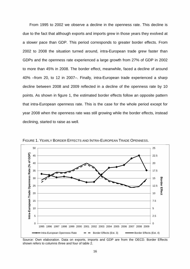
16
From 1995 to 2002 we observe a decline in the openness rate. This decline is
due to the fact that although exports and imports grew in those years they evolved at
a slower pace than GDP. This period corresponds to greater border effects. From
2002 to 2008 the situation turned around, intra-European trade grew faster than
GDPs and the openness rate experienced a large growth from 27% of GDP in 2002
to more than 45% in 2008. The border effect, meanwhile, faced a decline of around
40% –from 20, to 12 in 2007–. Finally, intra-European trade experienced a sharp
decline between 2008 and 2009 reflected in a decline of the openness rate by 10
points. As shown in figure 1, the estimated border effects follow an opposite pattern
that intra-European openness rate. This is the case for the whole period except for
year 2008 when the openness rate was still growing while the border effects, instead
declining, started to raise as well.
FIGURE 1. YEARLY BORDER EFFECTS AND INTRA-EUROPEAN TRADE OPENNESS.
Source: Own elaboration. Data on exports, imports and GDP are from the OECD. Border Effects shown refers to columns three and four of table 2.
0
2.5
5
7.5
10
12.5
15
17.5
20
22.5
25
0
5
10
15
20
25
30
35
40
45
50
1995 1996 1997 1998 1999 2000 2001 2002 2003 2004 2005 2006 2007 2008 2009
Bo
rder E
ffectIn
tra-
Eu
rop
ean
Tra
de
Op
enn
ess
Rat
e (%
of
GD
P)
Intra-European Openness Rate Border Effects (Est. 3) Border Effects (Est. 4)
17
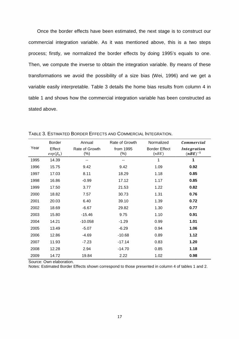
Once the border effects have been estimated, the next stage is to construct our
commercial integration variable. As it was mentioned above, this is a two steps
process; firstly, we normalized the border effects by doing 1995’s equals to one.
Then, we compute the inverse to obtain the integration variable. By means of these
transformations we avoid the possibility of a size bias (Wei, 1996) and we get a
variable easily interpretable. Table 3 details the home bias results from column 4 in
table 1 and shows how the commercial integration variable has been constructed as
stated above.
TABLE 3. ESTIMATED BORDER EFFECTS AND COMMERCIAL INTEGRATION.
Year Border Annual Rate of Growth Normalized ^_``abcdef Effect
G�g >h! Rate of Growth
(%) from 1995
(%) Border Effect
(KiR! jklambeld_k
kno!�p
1995 14.39 -- -- 1 1
1996 15.75 9.42 9.42 1.09 0.92
1997 17.03 8.11 18.29 1.18 0.85
1998 16.86 -0.99 17.12 1.17 0.85
1999 17.50 3.77 21.53 1.22 0.82
2000 18.82 7.57 30.73 1.31 0.76
2001 20.03 6.40 39.10 1.39 0.72
2002 18.69 -6.67 29.82 1.30 0.77
2003 15.80 -15.46 9.75 1.10 0.91
2004 14.21 -10.058 -1.29 0.99 1.01
2005 13.49 -5.07 -6.29 0.94 1.06
2006 12.86 -4.69 -10.68 0.89 1.12
2007 11.93 -7.23 -17.14 0.83 1.20
2008 12.28 2.94 -14.70 0.85 1.18
2009 14.72 19.84 2.22 1.02 0.98
Source: Own elaboration. Notes: Estimated Border Effects shown correspond to those presented in column 4 of tables 1 and 2.
18
For the purpose of this paper we have also addressed the border effect issue
from a country point of view by estimating the country-specific evolution of the home
bias over the period considered. Estimated border effects and commercial integration
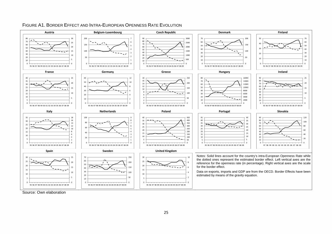
variables for each country are presented in table A2 and figure A1 in the appendix8.
3.2. GRAVITY MODEL FOR FDI. THE TRADE-FDI NEXUS
We analyse the impact of intra-European trade integration on the bilateral FDI
flows within the nineteen European countries using the gravity model specifications
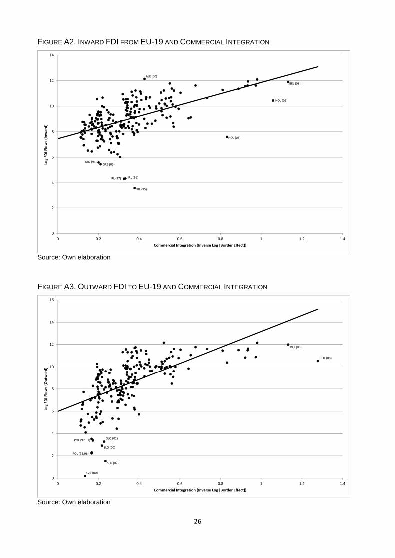
discussed above. Tentatively figures A2 and A3 in the appendix show the correlation
between commercial integration, computed as the inverse of the border effects
estimates, and FDI inflows and outflows respectively. More specifically, FDI for a
reporting country accounts for the logarithm of the aggregate flows to/from the rest of
the European countries in the sample. Both figures suggest a positive relationship
between FDI and Commercial Integration. Thus, we may expect a priori positive
estimates for the integration variables in the estimation of the gravity model for FDI.
The results of these regressions are presented in table 4. The results presented
in columns 1 and 3 correspond to the horizontal model shown in equation (5).
Estimates regarding home and host GDP are in line with earlier results from gravity
equations and are significant at 1% level. However, the horizontal (proximity-
concentration) model suggests that the coefficients on both GDP variables should be
equal to one. Yet, this is not supported by the data. The restriction on both
coefficients equals to unity is rejected at the 1% level in columns 1 and 3. We have
included the corruption perception index (CPI) from Transparency International as a
control variable. We do find significant impact of this index –for the host country– on
8 Complete estimation results are available from the authors upon request.
19
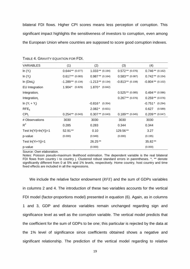
bilateral FDI flows. Higher CPI scores means less perception of corruption. This
significant impact highlights the sensitiveness of investors to corruption, even among
the European Union where countries are supposed to score good corruption indexes.
TABLE 4. GRAVITY EQUATION FOR FDI.
VARIABLES (1) (2) (3) (4)
ln (Yi) 0.644 ** (0.077) 1.033 ** (0.194) 0.572 ** (0.076) 0.746 ** (0.162)
ln (Yj) 0.617 ** (0.083) 0.987 ** (0.164) 0.583 ** (0.087) 0.742 ** (0.154)
ln (Distij) -1.289 ** (0.134) -1.213 ** (0.134) -0.813 ** (0.108) -0.804 ** (0.102)
EU Integration 1.904 * (0.829) 1.870 * (0.842)
Integrationi 0.525 ** (0.085) 0.494 ** (0.086)
Integrationj 0.267 ** (0.076) 0.259 ** (0.076)
ln (Yi + Yj) -0.816 * (0.354) -0.751 * (0.294)
RFEij 2.082 * (0.821) 0.627 (0.589)
CPIj 0.254 ** (0.043) 0.307 ** (0.043) 0.189 ** (0.045) 0.209 ** (0.047)
# Observations 3030 3030 3030 3030
R2 0.285 0.283 0.344 0.344
Test ln(Yi)=ln(Yj)=1 52.91 ** 0.10 129.56 ** 3.27
p-value (0.000) (0.949) (0.000) (0.195)
Test ln(Yi+Yj)=1 26.25 ** 35.82 **
p-value (0.000) (0.000)
Source: Own elaboration. Notes: Poisson pseudo-maximum likelihood estimation. The dependent variable is the real bilateral FDI flows from country i to country j. Clustered robust standard errors in parentheses. *, ** denote significantly different from 0 at 5% and 1% levels, respectively. Home country, host country and time fixed effects are included in all the regressions.
We include the relative factor endowment (QNR) and the sum of GDPs variables
in columns 2 and 4. The introduction of these two variables accounts for the vertical
FDI model (factor-proportions model) presented in equation (6). Again, as in columns
1 and 3, GDP and distance variables remain unchanged regarding sign and
significance level as well as the corruption variable. The vertical model predicts that
the coefficient for the sum of GDPs to be one; this particular is rejected by the data at
the 1% level of significance since coefficients obtained shows a negative and
significant relationship. The prediction of the vertical model regarding to relative
20
factor endowments is that FDI should increase in the high-skilled labour abundance
of the home country, relative to the host country. Evidence from the data is mixed
and inconclusive. While it may exert a positive impact in specification (2),
specification (4) shows a coefficient not significantly different form zero. In the case
of the European countries, home and host economic structures and human capital
endowments are quite similar so it is understandable that this measure will show
mixed evidence for this group of countries.
Finally and what is more interesting for the purpose of this paper, commercial
integration variables are included in all the regressions to account for the Trade-FDI
nexus. In column 1 and 3 the average commercial integration is suggested while in
columns 2 and 4 we consider the home and host country trade integration variables
separately. Results indicate a complementary relationship between intra-European
trade and FDI. This result is supported by the data in the four specifications
considered. The estimated coefficients are positive and statistically significant at 5%
in the cases of the average commercial integration variable. The evidence from the
home and host country variables is even stronger.
4. CONCLUSIONS
The empirical analysis carried out in this paper states that commercial
integration, captured by the evolution of the home bias, and FDI within the European
Union during 1995-2009 exhibit a positive correlation, thus displaying a relationship
of complementarity. The results also point out that cost differentials, for the country
sample considered, are not as relevant as the possibility of gaining market share.
The gravity equation for trade points out a positive and decreasing, up to 2007,
border effect, which means that in spite of the establishment of the Single Market Act
21
there is still a bias in favor of domestic goods. This bias, in the case of the EU, is
probably caused by informal trade barriers, features related to marginal propensity to
consume and the degree of substitution between goods.
Our findings support the idea that policies targeted to promote further
consolidations of the European Single Market –removing informal trade barriers,
promoting liberalization and reducing bureaucracy–, may have positive effects, not
only regarding the commercial performance of the EU but also helping to intensify
FDI flows among the European countries, and indirectly, stimulating economic
growth.
REFERENCES Agarwal (1980): “Determinants of Foreign Direct Investment: a Survey”,
Weltwirtschaftliches Archiv, 116, 739-773. Alguacil, M., Cuadros, A., and Orts, V. (2008): “EU Enlargement and Inward FDI”,
Review of Development Economics, 12, 594-604. Anderson, J. (1979): “A Theoretical Foundation of the Gravity Equation”, American
Economic Review, 69, 106-116. _____ and Van Wincoop, E. (2003): “Gravity with gravitas: a solution to the border
puzzle”, American Economic Review, 93, 170-192. Balasubramanyam, V., Salisu, M. and Sapsford, D. (1999): “Foreign Direct
Investment as an Engine of Growth”, Journal of International Trade and Economic Development, 8, 27-40.
Balasubramanian, V., Sapsford, D. and Griffiths, D. (2002): “Regional Integration Agreements and Foreign Direct Investment: Theory and Preliminary Evidence”, The Manchester School, 70, 460-482.
Bayoumi, T. and Lipworth, G. (1997): “Japanese Foreign Direct Investment and Regional Trade”, Finance and Development, 34, 11-13.
Bergstrand, J. (1985): “The Gravity Equation in International Trade: some Microeconomic Foundations and Empirical Evidence”, Review of Economics and Statistics, 67, 474-481.
_____ and Egger, P. (2007): “A Knowledge-and-Physical-Capital Model of International Trade Flows, Foreign Direct Investment, and Multinational Enterprises”, Journal of International Economics, 73, 278-308.
Blonigen, B. (2001): “In Search of Substitution between Foreign Production and Exports”, Journal of International Economics, 53, 81-104.
22
Brainard, S. (1997): “An Empirical Assessment of the Proximity-Concentration Trade-off between Multinational Sales and Trade”, American Economic Review, 87, 520-544.
Brenton, P., Di Mauro, F and Lucke, M (1999): “Economic Integration and FDI: an Empirical Analysis of Foreign Investment in the EU and in Central and Eastern Europe”, Empirica, 26, 95-121.
Buckley, P. and Casson, M. (1976): The Future of the Multinational Enterprise. Holmes & Meier Publishers. New York.
Caves, R. (1971): “International Corporations: The Industrial Economics of Foreign Investments”, Economica, 39, 1-27.
Chen, N. (2004): “Intra-national versus international trade in the European Union: why do national borders matter”, Journal of International Economics, 63, 93-118.
Cuadros, A., Orts, V,. and Alguacil, M. (2004): “Openness and Growth: Re-Examining Foreign Direct Investment, Trade and Output Linkages in Latin America”, The Journal of Development Studies, 40, 167-192.
Deardorff, A. (1998): “Determinants of Bilateral Trade: Does Gravity Work in a Neoclassical World?” in The Regionalization of the World Economy, 7-22. University of Chicago Press. Chicago.
Dunning, J. (1973): “The Determinants of International Production”, Oxford Economic Papers, 25, 289-336.
_____ (1981): International Production and the Multinational Enterprise. George Allen and Unwin. London.
Eaton, J. and Tamura, A. (1996): “Japanese and US Exports and Investment as Conduits of Growth”, NBER Working Paper No. 5457.
Egger, P and Pfaffermayer, M. (2004a): “Foreign Direct Investment and European Integration in the 1990s”, World Economy, 27, 99-110.
_____ and _____ (2004b): “Distance, Trade and FDI: A Hausman-Taylor SUR Approach”, Journal of Applied Econometrics, 19, 227-246.
Feenstra, R. (2002): “Border effects and the gravity equation: consistent method for estimation”, Scottish Journal of Political Economy, 49, 491-506.
Fillat-Castejón, C. Francois, J. and Wörz, J. (2008): “Cross-Border Trade and FDI in Services”, CEPR Discussion Paper No. 7074.
Goldberg, L. and Klein, M. (1999): “International Trade and Factor Mobility: an Empirical Investigation”, NBER Working Paper No. 7196.
Graham, E. (1996): “On the Relationship among Foreign Direct Investment and International Trade in the Manufacturing Sector: Empirical Results for the United States and Japan”, WTO Staff Working Paper RD-96-008.
Gourieroux, C., Monfort, A. and Trognon, A. (1984a): “Pseudo Maximum Likelihood Methods: Theory”, Econometrica, 52, 681-700.
_____, _____ and _____ (1984b): “Pseudo Maximum Likelihood Methods: Applications to Poisson Models”, Econometrica, 52, 701-720.
Head, K. and Mayer, T. (2002): “Illusory Border Effects: Distance Mismeasurement Inflates Estimates fo Home Bias in Trade”, CEPII Working Paper 2002-01.
23
_____ and Ries, J. (2001): “Increasing returns versus national product differentiation as an explanation for the pattern of US-Canada trade”, American Economic Review, 91, 858-876.
Helliwell, J. F. (1996): “Do national borders matter for Québec’s trade?”, Canadian Journal of Economics, 29, 507-522.
Hymer, S. (1976): The International Operations of National Firms: a Study of Foreign Direct Investment. MIT Press. Cambridge, MA.
Kleinert, J. and Toubal, F. (2010): “Gravity for FDI”, Review of International Economics, 18, 1-13.
Liu, X., Whalley, J. and Xin, X., (2010): “Non-tradable goods and the border effect puzzle”, Economic Modelling, 27, 909-914.
Martinez, V., Bengoa, M and Sanchez-Robles, B. (2012a): “Foreign Direct Investment and Trade: Complements or Substitutes? Empirical Evidence for the European Union”, Technology and Investment, 3, 105-112.
_____, _____ and _____ (2012b): “European Union and Trade Integration: Does the Home Bias Puzzle Matter?” Revista de Economia Mundial, 32, 173-188.
Markusen, J. and Maskus, K. (2002): “Discriminating among Alternative Theories of the Multinational Enterprise”, Review of International Economics, 10, 694-707.
McCallum, J. (1995): “National borders matter: Canada-US regional trade patterns”, American Economic Review, 37, 615-623.
Motta, M. and Norman, G. (1996): “Does Economic Integration Cause Foreign Direct Investment?” International Economic Review, 37, 757-783.
Mundell, R. (1957): “International Trade and Factor Mobility”, American Economic Review, 57, 321-335.
Nakamura, J. and Oyama, T. (1998): “The Determinants of Foreign Direct Investment from Japan and the United States to East Asian Countries and the Linkages between FDI and Trade”, Bank of Japan Working Paper No. 98-11.
Neary, J. (2009): “Trade Costs and Foreign Direct Investment”, International Review of Economics and Finance, 19, 207-218.
Nitsch, V. (2000): “National borders and international trade: evidence from the European Union”, Canadian Journal of Economics, 33, 1091-1105.
Pfaffermayer, M. (1996): “Foreign Outward Direct Investment and Exports I Austrian Manufacturing: Substitues or Complements?” Weltwirtschaftliches Archiv, 132,501-552.
Qian, Z. (2007): “FDI and European Economic Integration, Master dissertation, M. A. Economics of International Trade and European Integration”, mimeo, University of Antwerp, Belgium.
Sanna-Randaccio, F. (1996): “New Protectionism and Multinational Companies”, Journal of International Economics, 41, 29-51.
Santos Silva, J. and Tenreyro, S. (2006): “The Log of Gravity”, The Review of Economics and Statistics, 88, 641-658.
Swenson, D. (2004): “Foreign Investment and the Mediation of Trade Flows”, Review of International Economics, 12, 609-629.
Tinbergen, J. (1962): Shaping the World Economy: Suggestions for an International Economic Policy, Twentieth Century Fund, New York.
24
UNCTAD (2010a, 2011a): Trade and Development Report. United Nations. New York and Geneve.
_____ (2010b, 2011b): World Investment Report. United Nations. New York and Geneve.
Wei, S. (1996): “Intra-national versus international trade: how stubborn are nations in global integration”, NBER Working Paper No. 5531, Cambridge, MA.
Wolf, N. (2009): “Was Germany Ever United? Evidence from Intra- and International Trade”, The Journal of Economic History, 69, 846-881.
APPENDIX TABLE A1. SECTORS OF ACTIVITY.
1 2 3 4 5 6 7 8 9 10 11 12
Agriculture, forestry and fishing Mining and quarrying Food, beverages and tobacco Textiles, leather and footwear Wood and cork Pulp paper, printing and publishing Coke, refined petroleum and nuclear fuel Chemical excluding pharmaceuticals Pharmaceuticals Rubber and plastics Non-metallic products Basic metals
13 14 15 16 17 18 19 20 21 22 23
Fabricated metal products Machinery and equipment n.e.c Office, accounting and computing machinery Electrical machinery and apparatus n.e.c Radio TV communication equipment Medical precision and optical instrument Motor vehicles, trailers and semi-trailers Shipbuilding Aircraft and spacecraft Railroad and transport equipment n.e.c Manufacturing n.e.c and recycling
Source: Own elaboration
25
FIGURE A1. BORDER EFFECT AND INTRA-EUROPEAN OPENNESS RATE EVOLUTION Austria Belgium-Luxembourg Czech Republic Denmark Finland
France Germany Greece Hungary Ireland
Italy Netherlands Poland Portugal Slovakia
Spain Sweden United Kingdom
Notes: Solid lines account for the country’s intra-European Openness Rate while the dotted ones represent the estimated border effect. Left vertical axes are the reference for the openness rate (in percentage). Right vertical axes are the scale for the border effect.
Data on exports, imports and GDP are from the OECD. Border Effects have been estimated by means of the gravity equation.
Source: Own elaboration
0
5
10
15
20
25
30
0
10
20
30
40
50
60
70
80
95 96 97 98 99 00 01 02 03 04 05 06 07 08 09
0
1
2
3
4
5
6
7
0
50
100
150
200
95 96 97 98 99 00 01 02 03 04 05 06 07 08 09
0
500
1000
1500
2000
2500
3000
0
10
20
30
40
50
60
70
80
90
95 96 97 98 99 00 01 02 03 04 05 06 07 08 09
0
50
100
150
200
0
10
20
30
40
50
60
70
95 96 97 98 99 00 01 02 03 04 05 06 07 08 09
0
10
20
30
40
50
60
70
0
10
20
30
40
50
95 96 97 98 99 00 01 02 03 04 05 06 07 08 09
0
5
10
15
20
25
0
5
10
15
20
25
30
35
40
95 96 97 98 99 00 01 02 03 04 05 06 07 08 09
0
2
4
6
8
10
12
0
10
20
30
40
50
60
95 96 97 98 99 00 01 02 03 04 05 06 07 08 09
0
50
100
150
200
250
0
2
4
6
8
10
12
14
16
18
95 96 97 98 99 00 01 02 03 04 05 06 07 08 09
0
2000
4000
6000
8000
10000
12000
14000
16000
0
10
20
30
40
50
60
70
80
95 96 97 98 99 00 01 02 03 04 05 06 07 08 09
0
5
10
15
20
25
0
10
20
30
40
50
60
70
80
90
95 96 97 98 99 00 01 02 03 04 05 06 07 08 09
0
2
4
6
8
10
12
14
16
18
0
5
10
15
20
25
30
35
95 96 97 98 99 00 01 02 03 04 05 06 07 08 09
0
1
2
3
4
5
6
7
8
9
0
20
40
60
80
100
95 96 97 98 99 00 01 02 03 04 05 06 07 08 09
0
50
100
150
200
250
300
350
400
450
0
5
10
15
20
25
30
35
40
95 96 97 98 99 00 01 02 03 04 05 06 07 08 09
0
5
10
15
20
25
30
35
40
0
5
10
15
20
25
30
35
40
45
95 96 97 98 99 00 01 02 03 04 05 06 07 08 09
0
20
40
60
80
100
120
0
10
20
30
40
50
60
70
80
90
97 98 99 00 01 02 03 04 05 06 07 08 09
0
5
10
15
20
25
0
5
10
15
20
25
30
95 96 97 98 99 00 01 02 03 04 05 06 07 08 09
0
50
100
150
200
250
0
10
20
30
40
50
60
70
95 96 97 98 99 00 01 02 03 04 05 06 07 08 09
0
2
4
6
8
10
0
5
10
15
20
25
30
95 96 97 98 99 00 01 02 03 04 05 06 07 08 09
26
FIGURE A2. INWARD FDI FROM EU-19 AND COMMERCIAL INTEGRATION
Source: Own elaboration
FIGURE A3. OUTWARD FDI TO EU-19 AND COMMERCIAL INTEGRATION
Source: Own elaboration
0
2
4
6
8
10
12
14
0 0.2 0.4 0.6 0.8 1 1.2 1.4
Log
FD
I Flo
ws
(In
wa
rd)
Commercial Integration (Inverse Log [Border Effect])
IRL (96)IRL (97)
GRE (05)
BEL (08)
IRL (95)
HOL (09)
HOL (06)
ALE (00)
DIN (96)
0
2
4
6
8
10
12
14
16
0 0.2 0.4 0.6 0.8 1 1.2 1.4
Log
FD
I Flo
ws
(Ou
twa
rd)
Commercial Integration (Inverse Log [Border Effect])
POL (97,01)
POL (95,96)
SLO (00)
SLO (01)
SLO (02)
CZE (00)
HOL (08)
BEL (08)
Related Documents


![Fondo A151 Funtsa Francisco Bengoa Berbejillo INVENTARIO ......A151/A-101 Bengoa Berbejillo, Francisco de Adios [sic] a "Elema" = Agur "Elema" Partitura (1903-1977) A151/A-102 Bengoa](https://static.cupdf.com/doc/110x72/608d03eaa02d6212c65f55d7/fondo-a151-funtsa-francisco-bengoa-berbejillo-inventario-a151a-101-bengoa.jpg)