Using the National Training Center Instrumentation System ...

Dissertation

Using the National Training Center Instrumentation System to Aid Simulation-Based Acquisition

Andrew Cady

This document was submitted as a dissertation in September 2017 in partial fulfillment of the requirements of the doctoral degree in public policy analysis at the Pardee RAND Graduate School. The faculty committee that supervised and approved the dissertation consisted of Bryan Hallmark (Chair), Joe Martz, and Randall Steeb.

PARDEE RAND GRADUATE SCHOOL

For more information on this publication, visit http://www.rand.org/pubs/rgs_dissertations/RGSD406.html

Published 2018 by the RAND Corporation, Santa Monica, Calif.

R® is a registered trademark

Limited Print and Electronic Distribution Rights

This document and trademark(s) contained herein are protected by law. This representation of RAND intellectual property is provided for noncommercial use only. Unauthorized posting of this publication online is prohibited. Permission is given to duplicate this document for personal use only, as long as it is unaltered and complete. Permission is required from RAND to reproduce, or reuse in another form, any of its research documents for commercial use. For information on reprint and linking permissions, please visit www.rand.org/pubs/permissions.html.

The RAND Corporation is a research organization that develops solutions to public policy challenges to help make communities throughout the world safer and more secure, healthier and more prosperous. RAND is nonprofit, nonpartisan, and committed to the public interest.

RAND’s publications do not necessarily reflect the opinions of its research clients and sponsors. The views expressed in this dissertation are those of the author and do not represent the official policy or position of the United States Air Force, or the U.S. Government.

Support RAND Make a tax-deductible charitable contribution at

www.rand.org/giving/contribute

www.rand.org

iii

Abstract

Though current data sources for simulation models used in the United States Department of Defense (DoD) acquisition process are many and varied, none adequately represents how weapon systems behave in combat in a robust, quantifiable manner, leading to uncertainty in the acquisition decision making process. The objective of this dissertation is to improve this process by developing empirically derived measures of direct fire behaviors from U.S. Army National Training Center (NTC) data and by demonstrating how these measures can be used to support acquisition decisions based on the output of simulation-based modeling. To accomplish this, I employ a three-part methodology.

First, I identify the current data sources for models and simulations used in the defense acquisition process. Of these four data sources—historical combat, operational testing, other simulations, and subject matter expert (SME) judgment—no single source can adequately describe combat behaviors of weapon systems across a wide range of operational environments.

Second, I turn to the NTC data as a potential solution to this gap in data sources. I first examine prior NTC-based research and lessons this literature holds for current and future research. I examine the doctrinal underpinnings of maneuver combat behaviors, deriving five important aspects of direct fire—two of which are operationalized in this dissertation: direct fire engagement and movement and maneuver. I examine the NTC instrumentation system data generation process, strengths, and drawbacks to determine if it could measure these. Finally, I describe four measures that I derive to describe maneuver combat behavior—weapon system probability of hit, weapon system rate of fire, unit dispersion, and unit speed.

Third, I compare the measures derived in this dissertation against baseline measures from the Joint Conflict and Tactical Simulation (JCATS) simulation model to determine the difference the two sources of measures – actual NTC behavior and JCATS baseline - make in three outcomes: exchange ratio, drawdown of forces rate, and volume of fire. To perform this comparison, I create a scenario based on prior simulation studies along with four excursions to test the influence of changes in mission, enemy, and terrain on the impact of data source. I analyze the results of 300 runs of the JCATS model using a series of linear regressions. For each excursion, regression models indicate a highly significant effect of data source on each model outcome.

I conclude this dissertation with a recommendation that the measures described herein form the basis for a larger system of NTC-based behavioral measurement for modeling and simulation (M&S) data. I also recommend several software and hardware improvements to the NTC instrumentation system that could improve its utility as both a data source and a training resource. As future research, I recommend applying advanced analytic techniques to these data, applying these methods to other combat training centers and applying these measures to training and tactics development.

v

Table of Contents

Abstract .......................................................................................................................................... iiiTable of Contents ............................................................................................................................ vFigures........................................................................................................................................... viiTables ............................................................................................................................................. ixAcknowledgements ........................................................................................................................ xiAbbreviations ............................................................................................................................... xiii1. Introduction ................................................................................................................................. 1

Background............................................................................................................................................... 1Objective .................................................................................................................................................. 3Structure of This Dissertation ................................................................................................................... 4Limitations ................................................................................................................................................ 7

2. Current Sources of Data for Combat Simulation Modeling ....................................................... 8Introduction .............................................................................................................................................. 8Historical Combat ..................................................................................................................................... 9Operational Testing ................................................................................................................................ 14Other Simulations ................................................................................................................................... 16SME Judgment ....................................................................................................................................... 21Discussion and Summary of Existing Data Sources............................................................................... 25

3. Deriving Behavioral Combat Measures from NTC-IS ............................................................. 27What Is the NTC and How Can Its Data Be Useful? ............................................................................. 27Historical Methods for Analyzing the NTC-IS ...................................................................................... 29Doctrinal Overview of Key Behavioral Aspects of Direct Fire ............................................................. 39NTC-IS Data Overview .......................................................................................................................... 47Deriving Measures of Direct Fire Planning and Execution .................................................................... 53Discussion .............................................................................................................................................. 59

4. Testing the Difference in JCATS Model Outcomes from Using NTC-based Data .................. 60Model Selection ...................................................................................................................................... 60Variable Selection .................................................................................................................................. 61Experimental Design .............................................................................................................................. 65Analysis Methodology ............................................................................................................................ 72Model Results ......................................................................................................................................... 73Discussion .............................................................................................................................................. 90

5. Conclusions and Policy Recommendations .............................................................................. 92Conclusions ............................................................................................................................................ 92Policy Recommendations ....................................................................................................................... 94Suggestions for Additional Research ..................................................................................................... 97

Appendix A: Pairing Fires and Hits in NTC-IS .......................................................................... 100

vi

Initial Fire-Hit Pairing .......................................................................................................................... 102Advanced Fire-Hit Pairing ................................................................................................................... 106Contact Creation ................................................................................................................................... 111Indirect Fire Advanced Pairing ............................................................................................................. 115

Appendix B: Line of Sight Algorithm Description and Assumptions ........................................ 117Appendix C: Additional NTC-IS Measures Not Tested in this Research .................................. 120Appendix D: Verification and Validation of the NTC-IS Data .................................................. 125

Conceptual Model Validation ............................................................................................................... 127Computerized Model Verification ........................................................................................................ 127Operational Validation ......................................................................................................................... 135

Appendix E: Full Results of NTC-IS Analysis ........................................................................... 151Appendix F: Regression Model Specifications and Diagnostics ................................................ 152

Experimental Design Matrices ............................................................................................................. 152Regression Equations ........................................................................................................................... 154Model Diagnostics ................................................................................................................................ 155

Works Cited ................................................................................................................................ 163

vii

Figures

Figure 2.1. Spectrum of Combat Simulations ............................................................................... 16Figure 3.1: MILES Beam Diffusion Patterns ............................................................................... 49Figure 4.1: Scenario Sampling Design ......................................................................................... 68Figure A.1: Fire-Hit Pairing Process .......................................................................................... 101Figure A.2: Initial Fire-Hit Pairing ............................................................................................. 105Figure A.3: Advanced Fire-Hit Pairing ...................................................................................... 110Figure A.4: Contact Creation ...................................................................................................... 114Figure A.5: Advanced Indirect Fire Pairing ............................................................................... 116Figure B.1: Line of Sight Data Resolution Correction ............................................................... 118Figure D.1: Model Validation Framework ................................................................................. 125Figure D.2: Significance levels with varying window duration: all weapon systems ................ 149Figure D.3: Significance levels with varying window duration: Tanks ..................................... 149Figure D.4: Significance levels with varying window duration: IFVs ....................................... 150Figure F.1: Exchange Ratio Q-Q Plot ......................................................................................... 156Figure F.2: Exchange Ratio Model Residuals ............................................................................ 157Figure F.3: Exchange Ratio Log-Linear Q-Q Plot ...................................................................... 157Figure F.3: Drawdown of Forces Rate Q-Q Plot ........................................................................ 158Figure F.4: Rate of Fire Linear Q-Q Plot .................................................................................... 159Figure F.5: Rate of Fire Log-Linear Q-Q Plot ............................................................................ 160Figure F.6: Quantity of Fire Linear Q-Q Plot ............................................................................. 161Figure F.7: Quantity of Fire Log-Linear Q-Q Plot ..................................................................... 162

ix

Tables

Table 1.1: List of NTC-IS Derived Measures ................................................................................. 5Table 1.2: Crosswalk of NTC-IS and JCATS Measures ................................................................ 5Table 1.3: JCATS Output Measures ............................................................................................... 6Table 2.1: Summary of Existing Data Sources ............................................................................. 25Table 3.1: List of De-Identified Data Fields ................................................................................. 52Table 3.2: List of NTC-IS Derived Measures ............................................................................... 55Table 4.1: Weapon Systems and Munition Types for Rate of Fire Data Modification ................ 63Table 4.2: Excursion Specifications ............................................................................................. 68Table 4.3: Summary of Experimental Design Effect Estimation ................................................. 70Table 4.4: Aliasing Structure for Design A .................................................................................. 71Table 4.5: Aliasing Structure for Design B .................................................................................. 71Table 4.6: Summary of Mission Variable Effects on JCATS Excursions .................................... 71Table 4.7: Summary of Observed Force Exchange Ratios ........................................................... 73Table 4.8: Regression Results: Effects on Force Exchange Ratio ................................................ 75Table 4.9: Kills by Side and Enemy Variable Setting .................................................................. 76Table 4.10: Observed Values of Drawdown of Forces Rate ........................................................ 77Table 4.11: Regression Results – Effects on Drawdown of Forces Rate ..................................... 78Table 4.12: Model Estimates of Drawdown of Force Rate by Side and Input Source ................. 79Table 4.13: Effect of Input Source with Enemy Interactions ....................................................... 80Table 4.14: Observed Values of Rate of Fire ............................................................................... 81Table 4.15: Regression Results: Effects on Rate of Fire .............................................................. 82Table 4.16: Model Estimates of Rate of Fire by Side and Input Source ...................................... 83Table 4.17: Rate of Fire—Effect of Input Source with Mission Interactions ............................... 84Table 4.18: Rate of Fire—Effect of Input Source with Enemy Interactions ................................ 84Table 4.19: Rate of Fire—Effect of Input Source with Terrain Interactions ................................ 85Table 4.20: Observed Values of Quantity of Fire ......................................................................... 86Table 4.21: Regression Results: Effects on Quantity of Fire ........................................................ 86Table 4.22: Model Estimates of Quantity of Fire by Side and Input Source ................................ 88Table 4.23: Quantity of Fire—Effect of Input Source with Mission Interactions ........................ 88Table 4.24: Quantity of Fire—Effect of input Source with Enemy Interactions .......................... 89Table 4.25: Quantity of Fire—Effect of Input Source with Terrain Interactions ......................... 89Table D.1: Initial Fire-Hit Pairing Assumptions ......................................................................... 129Table D.2: Advanced Fire-Hit Pairing Assumptions .................................................................. 130Table D.3: Contact Creation Assumptions ................................................................................. 131Table D.4: Initial Fire-Hit Pairing: First and Total Order Effect Statistics ................................ 133

x

Table D.5: Advanced Fire-Hit Pairing: First and Total Order Effect Statistics .......................... 133Table D.6: Contact Creation: First and Total Order Effect Statistics ......................................... 134Table D.7: All non-BMP Companies–Effect Sizes and Significance for Overall Probability of Hit

............................................................................................................................................. 139Table D.8: M1 Abrams–Effect Sizes and Significance for Overall Probability of Hit .............. 140Table D.9: T-80–Effect Sizes and Significance for Overall Probability of Hit .......................... 140Table D.10: M2/3 Bradley–Effect Sizes and Significance for Overall Probability of Hit ......... 141Table D.12: Tanks—Effect Sizes and Significance for Rate of Fire .......................................... 143Table D.13: IFVs—Effect Sizes and Significance for Rate of Fire ............................................ 143Table D.15: Effect Sizes and Significance for Unit Dispersion ................................................. 146Table D.17: Effect Sizes and Significance for Unit Speed ......................................................... 148Table D.18: IFVs—Effect Sizes and Significance for Unit Speed ............................................. 148Table D.19: Tanks—Effect Sizes and Significance for Unit Speed ........................................... 148Table F.1: Design A Data Matrix ............................................................................................... 152Table F.2: Design B Data Matrix ................................................................................................ 152

xi

Acknowledgements

As with any dissertation, this was far from a lonely effort. A great many people had a hand in making this document and this research a success—more than can possibly be listed here. I would first like to thank the other graduate students at the Pardee RAND Graduate School, particularly Stefan Zavislan, Chris Carson, and Dan Basco, for the homework help, life advice, and commiseration that make the time here worthwhile. Several instructors here also shaped by analytic toolbox and gave me the requisite skills to complete this dissertation in the extremely short time available, particularly Bart Bennett, Jeffrey Wasserman, and Chris Nelson. Connor Jackson was along for nearly every step of the journey, and was instrumental in helping to keep the vast amount of Python code required for this dissertation running.

I would next like to thank my committee chair, Bryan Hallmark. Through my entire time at RAND, I have worked for and with Bryan on a wide variety of projects. Through it all, his expertise, advice, and mentorship have proved invaluable in my growth as a policy analyst and in this dissertation. Without Bryan, this would not have been possible. I would also like to thank the other members of my committee, Randy Steeb and Lt Gen (ret.) Joe Martz. Their guidance and advice through the dissertation process has kept my on the right path, despite my best efforts to dive down every rabbit hole I encountered. I also could not have finished this dissertation on time were it not for the incredible help of Morgan Kisselburg, the RAND resident JCATS Jedi Master. Finally, I am very grateful for the support I received from the RAND Arroyo Center.

I would like to thank the leaders, soldiers and civilians at U.S. Army Forces Command and the National Training Center. I thank General Robert B. Abrams and Lieutenant General Patrick J Donahue II, the Commander and Deputy Commander of Forces Command for their support. Also, I thank Chief Warrant 5 John Robinson, Mr. Kirk Palan and Ms. Kristin Blake for their assistance at several key points in this research process. At the National Training Center, I appreciate the support of Major General Joseph Martin and Brigadier General Jeffrey Broadwater, the former and current commanders of the Center. Joe Moore and Maurice Marchbanks at the Raytheon Warrior Training Alliance provided invaluable help with the NTC-Instrumentation System and database. Sam Mallon helped work through many kinks, uncertainties, and bizarre data questions that I came up with during the course of this research.

Finally, I would like to thank my girlfriend, Irina. Over the past three years, I’ve probably spent more time talking to her about this dissertation than I have actually writing it. She gave me substantive, editorial, and most importantly, moral support every step of the way.

xiii

Abbreviations

AoA Analysis of Alternatives

ACR Armored Cavalry Regiment

ADP Army Doctrine Publication

ADRP Army Doctrine Reference Publication

AMSAA US Army Materiel Systems Analysis Activity

AR Army Regulation

ARI Army Research Institute for the Behavioral and Social Sciences

ATGM Anti-Tank Guided Missile

ATP Army Techniques Publication

AVCATT Aviation Combined Arms Tactical Trainer

BCT Brigade Combat Team

BEB Brigade Engineer Battalion

B-FIST Bradley Fire Support Team Vehicle

BFV Bradley Fighting Vehicle

BLUEFOR Blue Forces (generally referring to U.S. forces)

BSB Brigade Support Battalion

CAB Combined Arms Battalion

CALL Center for Army Lessons Learned

CBO Congressional Budget Office

CCTT Close Combat Tactical Trainer

COA Course Of Action

COMBATXXI Combined Arms Analysis Tool for the 21st Century

CSSB Combat Sustainment Support Battalion

CTC Combat Training Center

DATE Decisive Action Training Environment

DoD Department of Defense

xiv

FA Field Artillery

FIST Fire Support Team

FM Field Manual

FO Forward Observer

FORSCOM Forces Command

FOUO For Official Use Only

FSO Fire Support Officer

GCV Ground Combat Vehicle

GPS Global Positioning System

HHC Headquarters and Headquarters Company

ICV Infantry Carrier Vehicle

ID Identity

IFV Infantry Fighting Vehicle

JCATS Joint Conflict and Tactical Simulation

JMRC Joint Multinational Readiness Center

JRTC Joint Readiness Training Center

METL Mission Essential Task List

METT-TC Mission, Enemy, Terrain, Time, Troops and Support Available, Civil Considerations

MDMP Military Decision-Making Process

MILES Multiple Integrated Laser Engagement System

MOUT Military Operations in Urban Terrain

M&S Modeling and Simulation

NDV Non-Developmental Vehicle

NTC National Training Center

NTC-IS National Training Center Instrumentation System

OCT Observer Coach Trainer

OneSAF One Semi-Automated Forces

OPFOR Opposing Force (generally refers to anti-U.S. forces)

xv

OT&E Operational Testing and Evaluation

PH Probability of Hit

PK Probability of Kill

Q-Q Quantile-Quantile

RADGUNS Radar Directed Gun System Simulation

RPG Recommended Practices Guide

SAWE Simulation of Area Weapons Effects

SIMNET Simulator Networking

SME Subject Matter Expert

SRTM Shuttle Radar Topography Mission

SURVIAC Survivability/Vulnerability Information Analysis Center

TAFF Training Analysis and Feedback Facility

TESS Tactical Engagement Simulation System

TOW Tube-launched, Optically-tracked, Wire-guided Antitank Missile

TRADOC Training and Doctrine Command

TRAC TRADOC Analysis Command

U Unclassified

V&V Verification and Validation

1

1. Introduction

Background

Nearly every major Army acquisition decision is supported by the output of simulation models. These models enable the Army to understand how changes to weapons, organization, or tactics would affect the behavior and outcomes of future formations. Simulation models require accurate input data and model algorithms to produce useful results; however, in many cases, accurate input data based on actual behaviors of soldiers in combat or near-real combat conditions are not available. As a result, senior leaders may not trust the output of the simulation process or, worse yet, they might make a decision based on erroneous information.

A salient example of this is the Army’s recent Ground Combat Vehicle (GCV) acquisition program.1 This program, which sought to acquire a replacement to the M2/M3 Bradley Infantry Fighting Vehicle (IFV), included a large modeling and simulation (M&S) effort in several Analyses of Alternatives (AoAs) conducted by both the Training and Doctrine Command (TRADOC) Analysis Center (TRAC) and the Congressional Budget Office (CBO).2 One problem analysts quickly discovered in these studies was the lack of quantitative data on the effect of vehicle carrying capacity on combat outcomes. One of the chief arguments for replacing the Bradley in favor of the GCV was the larger capacity of the latter—the former fit a full 9-soldier squad rather than the 7-soldier carrying capacity of the legacy vehicle.3 Although the Army widely perceives that a vehicle carrying a full 9-soldier squad would enable more effective infantry employment than the current situation in which the squad must be split up among two vehicles,4 there was no reliable combat or test data describing the difference in effectiveness between the two configurations. This lack of accurate parameters was manifest in the results of the simulations: the Army and CBO’s simulations came to different conclusions about optimal choices from among the alternatives examined in the process, which was partially because of differences in opinion and data about the effect of a larger crew compartment.5

1Although this program was ultimately cancelled, a large amount of resources were invested in research and development to determine the program’s objectives and alternatives. 2Garrett R. Lambert et al., "Ground Combat Vehicle (GCV) Analysis of Alternatives (AoA) Final Report," (White Sands Missile Range, NM: TRADOC Analysis Center, 2011). Not available to the general public; "The Army's Ground Combat Vehicle Program and Alternatives," (Congressional Budget Office, 2013). 3"The Army's Ground Combat Vehicle Program and Alternatives." 4For an interesting discussion of the nine-soldier squad, see Bruce J. Held et al., "Understanding Why a Ground Combat Vehicle that Carries Nine Dismounts is Important to the Army," (Santa Monica, CA: RAND Corporation, 2013). 5Michael Hoffman, "Army, Industry Slam CBO's Scathing GCV Report," DoD Buzz 2013.

2

To estimate the effect of vehicle carrying capacity on combat performance, the Army conducted a series of live operational tests with a 7-soldier vehicle, the M2 Bradley IFV, and a 9-soldier alternative, the M1126 Stryker Infantry Carrier Vehicle (ICV).6 This test took place over two weeks and involved two different platoons in a two different operational scenarios. The study ultimately concluded that on most metrics as measured by a survey instrument, the 9-soldier configuration was superior to the 7-soldier.7 Although this analysis proved the ways in which a larger carrying capacity was valuable, it did not do so in a way that enabled future simulation modelers to quantify these ways and use them in future simulation models. This shortcoming can be seen in the controversy over the CBO report, which was published over a year after the experiment’s completion. Despite using several different weights for the relative importance of a larger crew compartment, the report still took criticism for its modeling methodology.

This episode demonstrates the broad uncertainty about the effect that many acquisition requirements have. In this example, simulation modelers found themselves unsure of the effect that a larger carrying capacity would have on the behavior of a hypothetical IFV. Later in the GCV acquisition program, the Army had to conduct a second series of operational tests to estimate performance parameters for Non-Developmental Vehicles (NDVs) under consideration, including a German and an Israeli IFV. In both cases, the operational tests, an expensive and slow means of gathering information, lengthened the overall process and did not completely stamp out controversy about expected behaviors for each weapon system.8

Because of the increasing complexity of weapon systems, defense acquisition programs rely more and more on detailed and accurate M&S to test the many disparate parts of a new program.9 Furthermore, testing designed to derive data for simulation models is increasingly becoming a cause of acquisition schedule delay, 10 In some cases, the only way these systems can

6The Army also considered using a closed-form simulation to determine the effect of a larger vehicle carrying capacity, but ultimately deemed an operational test to be the best analytical venue. 7Training and Doctrine Command Analysis Center, "Ground Combat Vehicle (GCV) Soldier Carrying Capacity Experiment," (White Sands Missile Range, NM2011). Not available to the general public. 8Hoffman, "Army, Industry Slam CBO's Scathing GCV Report."; Scott R. Gourley, "CBO Report on Ground Combat Vehicle Neglects Army data," Defense Media Network 2013., "The Army's Ground Combat Vehicle Program and Alternatives." 9For a description of this concept and an example using the Joint Strike Fighter program (the largest defense acquisition program to date), see Randy C. Zittel, "The Reality of Simulation-Based Acquisition--And an Example of US Military Implementation," Acquisition Review Quarterly 8, no. 2 (2001). 10Bernard Fox et al., "Test and Evaluation Trends and Costs for Aircraft and Guided Weapons," (Santa Monica, CA: RAND Corporation, 2004). John V. Farr, William R. Johnson, and Robert P. Birmingham, "A Multitiered Approach to Army Acquisition," Defense Acquisition Review Journal 12.2 (2005).

3

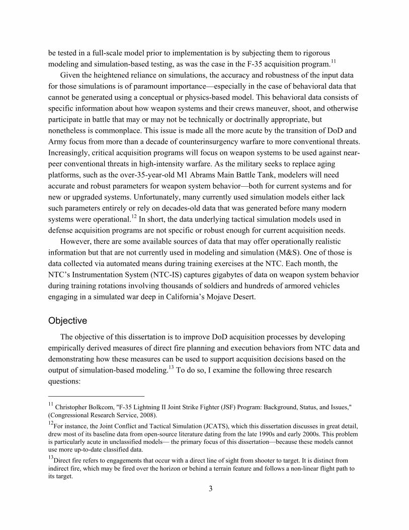
be tested in a full-scale model prior to implementation is by subjecting them to rigorous modeling and simulation-based testing, as was the case in the F-35 acquisition program.11

Given the heightened reliance on simulations, the accuracy and robustness of the input data for those simulations is of paramount importance—especially in the case of behavioral data that cannot be generated using a conceptual or physics-based model. This behavioral data consists of specific information about how weapon systems and their crews maneuver, shoot, and otherwise participate in battle that may or may not be technically or doctrinally appropriate, but nonetheless is commonplace. This issue is made all the more acute by the transition of DoD and Army focus from more than a decade of counterinsurgency warfare to more conventional threats. Increasingly, critical acquisition programs will focus on weapon systems to be used against near-peer conventional threats in high-intensity warfare. As the military seeks to replace aging platforms, such as the over-35-year-old M1 Abrams Main Battle Tank, modelers will need accurate and robust parameters for weapon system behavior—both for current systems and for new or upgraded systems. Unfortunately, many currently used simulation models either lack such parameters entirely or rely on decades-old data that was generated before many modern systems were operational.12 In short, the data underlying tactical simulation models used in defense acquisition programs are not specific or robust enough for current acquisition needs.

However, there are some available sources of data that may offer operationally realistic information but that are not currently used in modeling and simulation (M&S). One of those is data collected via automated means during training exercises at the NTC. Each month, the NTC’s Instrumentation System (NTC-IS) captures gigabytes of data on weapon system behavior during training rotations involving thousands of soldiers and hundreds of armored vehicles engaging in a simulated war deep in California’s Mojave Desert.

Objective

The objective of this dissertation is to improve DoD acquisition processes by developing empirically derived measures of direct fire planning and execution behaviors from NTC data and demonstrating how these measures can be used to support acquisition decisions based on the output of simulation-based modeling.13 To do so, I examine the following three research questions:

11 Christopher Bolkcom, "F-35 Lightning II Joint Strike Fighter (JSF) Program: Background, Status, and Issues," (Congressional Research Service, 2008). 12For instance, the Joint Conflict and Tactical Simulation (JCATS), which this dissertation discusses in great detail, drew most of its baseline data from open-source literature dating from the late 1990s and early 2000s. This problem is particularly acute in unclassified models— the primary focus of this dissertation—because these models cannot use more up-to-date classified data. 13Direct fire refers to engagements that occur with a direct line of sight from shooter to target. It is distinct from indirect fire, which may be fired over the horizon or behind a terrain feature and follows a non-linear flight path to its target.

4

1. Is NTC data better than existing simulation data sources? I first identify what the current data sources are for models and simulations used in the defense acquisition process. I then compare the NTC data against this status quo to determine which more accurately represents direct fire, company-level maneuver combat behaviors.

2. How can NTC data be leveraged as a simulation data source? This dissertation is by no means the first research effort that has sought to measure combat using NTC data. In this section, I seek to learn the lessons of prior attempts to create measures of combat behavior from NTC data to craft a new, more robust methodology for extracting measures.

3. What difference does the use of NTC data make in simulation model outcomes? Using a new data source is only worth the time and effort if doing so makes a meaningful difference in model outcomes. To determine this difference, I use a scenario and several excursions created with the Joint Conflict and Tactics Simulation (JCATS) entity-level combat simulation model.

By showing that the NTC data are superior to the status quo data sources, that it is possible to extract measures of combat behavior from the NTC, and that such measures make a meaningful difference in model outcomes compared with status quo data, this dissertation concludes that the acquisition process could be improved by using NTC data for models and simulations.

Structure of This Dissertation

In the following sections, I outline the structure of the dissertation, including methodologies employed to answer each of the research questions, as well as associated caveats.

Is NTC Data Better Than Existing Simulation Data Sources?

I address this question in Chapter 2 with an extensive literature review pertaining to Army simulation models and parameters derived from them. There are four current sources of simulation input data—historical analysis, operational testing, virtual simulations, and subject-matter expert (SME) judgment. Each of these data sources is compared on the basis of its quantity, specificity, and realism.

How Can the NTC Be Leveraged As a Simulation Data Source?

Based on the need identified in the literature review of existing data sources, I turn to the NTC-IS and quantitative measures of combat behavior in Chapter 3. I outline a new method for deriving measures of combat behavior from NTC data. I first examine past studies that have attempted to use NTC-IS to derive such behaviors, including work done by RAND Arroyo Center, the Army Research Institute for the Behavioral and Social Science (ARI), and the Center for Army Lessons Learned (CALL). From this review, I conclude that prior research involving

5

NTC data was unsuitable for deriving quantitative, micro-level measures of direct fire behaviors. Next, I analyze Army doctrine and relevant training literature to determine five important aspects of direct fire that can inform future simulation model parameters. These aspects are direct fire control, combined arms integration, pre-combat preparation, direct fire engagement, and movement and maneuver, although only measures describing the last two are created in this dissertation.

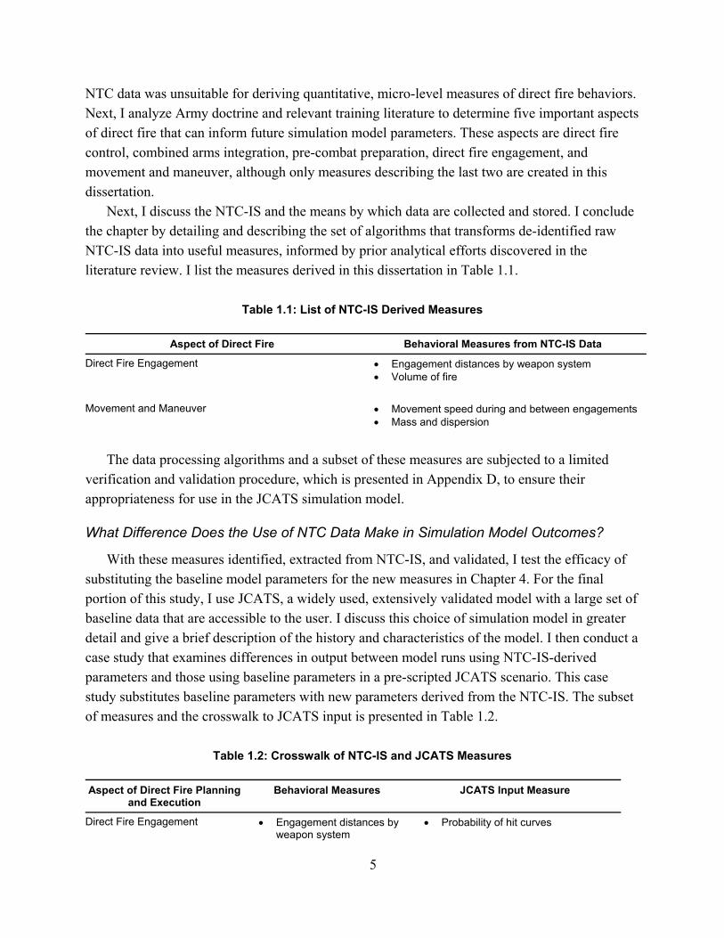
Next, I discuss the NTC-IS and the means by which data are collected and stored. I conclude the chapter by detailing and describing the set of algorithms that transforms de-identified raw NTC-IS data into useful measures, informed by prior analytical efforts discovered in the literature review. I list the measures derived in this dissertation in Table 1.1.

Table 1.1: List of NTC-IS Derived Measures

The data processing algorithms and a subset of these measures are subjected to a limited

verification and validation procedure, which is presented in Appendix D, to ensure their appropriateness for use in the JCATS simulation model.

What Difference Does the Use of NTC Data Make in Simulation Model Outcomes?

With these measures identified, extracted from NTC-IS, and validated, I test the efficacy of substituting the baseline model parameters for the new measures in Chapter 4. For the final portion of this study, I use JCATS, a widely used, extensively validated model with a large set of baseline data that are accessible to the user. I discuss this choice of simulation model in greater detail and give a brief description of the history and characteristics of the model. I then conduct a case study that examines differences in output between model runs using NTC-IS-derived parameters and those using baseline parameters in a pre-scripted JCATS scenario. This case study substitutes baseline parameters with new parameters derived from the NTC-IS. The subset of measures and the crosswalk to JCATS input is presented in Table 1.2.

Table 1.2: Crosswalk of NTC-IS and JCATS Measures

Aspect of Direct Fire Behavioral Measures from NTC-IS Data

Direct Fire Engagement Engagement distances by weapon system Volume of fire

Movement and Maneuver Movement speed during and between engagements Mass and dispersion

Aspect of Direct Fire Planning and Execution

Behavioral Measures JCATS Input Measure

Direct Fire Engagement Engagement distances by weapon system

Probability of hit curves

6

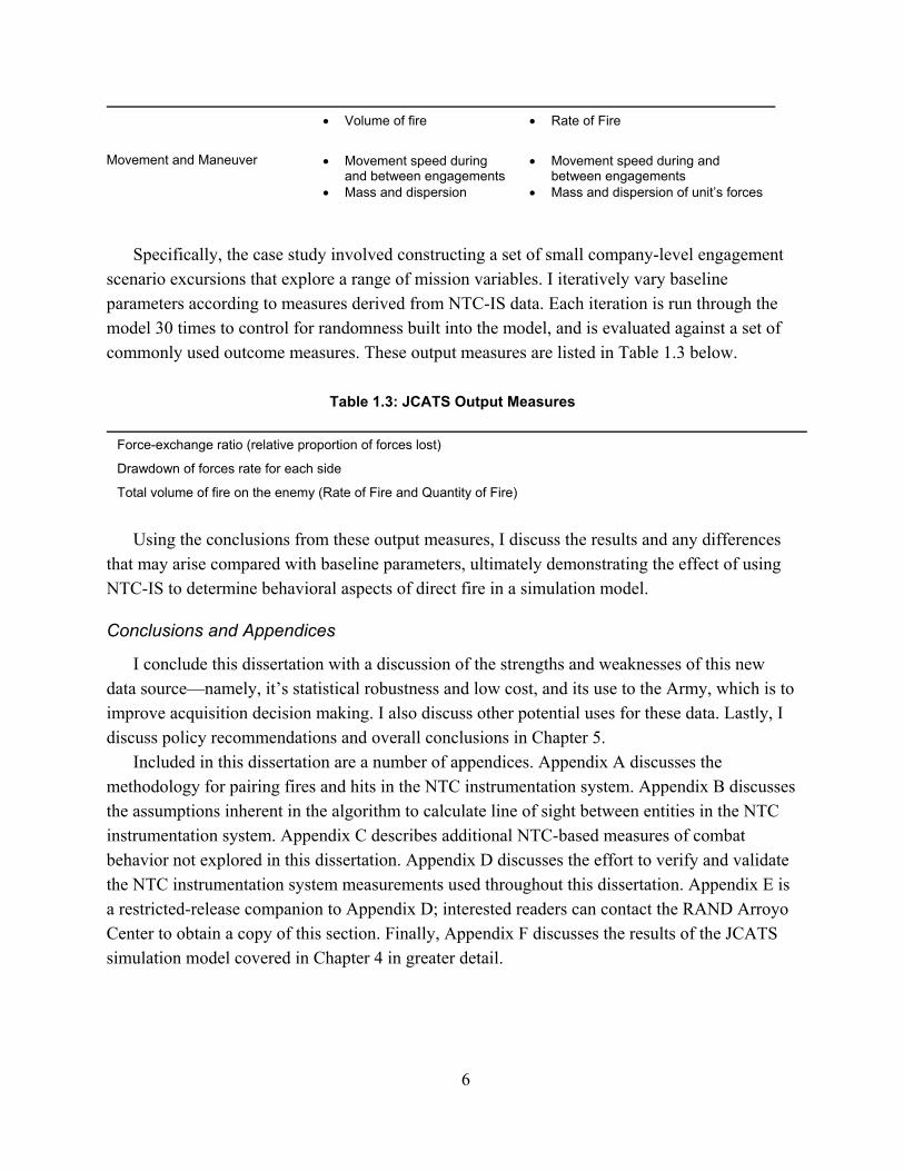
Specifically, the case study involved constructing a set of small company-level engagement

scenario excursions that explore a range of mission variables. I iteratively vary baseline parameters according to measures derived from NTC-IS data. Each iteration is run through the model 30 times to control for randomness built into the model, and is evaluated against a set of commonly used outcome measures. These output measures are listed in Table 1.3 below.

Table 1.3: JCATS Output Measures

Using the conclusions from these output measures, I discuss the results and any differences

that may arise compared with baseline parameters, ultimately demonstrating the effect of using NTC-IS to determine behavioral aspects of direct fire in a simulation model.

Conclusions and Appendices

I conclude this dissertation with a discussion of the strengths and weaknesses of this new data source—namely, it’s statistical robustness and low cost, and its use to the Army, which is to improve acquisition decision making. I also discuss other potential uses for these data. Lastly, I discuss policy recommendations and overall conclusions in Chapter 5.

Included in this dissertation are a number of appendices. Appendix A discusses the methodology for pairing fires and hits in the NTC instrumentation system. Appendix B discusses the assumptions inherent in the algorithm to calculate line of sight between entities in the NTC instrumentation system. Appendix C describes additional NTC-based measures of combat behavior not explored in this dissertation. Appendix D discusses the effort to verify and validate the NTC instrumentation system measurements used throughout this dissertation. Appendix E is a restricted-release companion to Appendix D; interested readers can contact the RAND Arroyo Center to obtain a copy of this section. Finally, Appendix F discusses the results of the JCATS simulation model covered in Chapter 4 in greater detail.

Volume of fire

Rate of Fire

Movement and Maneuver Movement speed during and between engagements

Mass and dispersion

Movement speed during and between engagements

Mass and dispersion of unit’s forces

Force-exchange ratio (relative proportion of forces lost)

Drawdown of forces rate for each side

Total volume of fire on the enemy (Rate of Fire and Quantity of Fire)

7

Limitations

Before continuing, I would like to note a few caveats and limitations of this work. First and foremost, this dissertation presents a proof of concept—it is neither possible nor recommended for an Army user to take the measures and computer code created in this dissertation and put them to immediate use. Rather, I present one possible way forward, discuss its strengths and weaknesses, and provide direction for future researchers and practitioners. Second, this dissertation focuses exclusively on armored and mechanized infantry units at the company level, because these weapon systems and unit types generate reliable data at the NTC. Similarly, the measures derived represent only a small subset of the behavioral measures possible from the NTC instrumentation system. Many more could be derived—and for other weapon systems and unit types—if additional resources, expertise, and computational power were at the researcher’s disposal, to include other NTC-based data sources beyond the instrumentation system.14 Third, the JCATS scenario tested in this dissertation represents only a small subset of the possible missions and scenarios a modeler could use. It is not intended to be representative of all combat scenarios, but rather to provide insight into potential effects of this system with some small degree of qualitative generalizability. Fourth, this dissertation exclusively discussed data from the NTC—three other maneuver combat training centers (CTCs) exist,15 they are not examined. Finally, this research does not intend to evangelize NTC data as the best possible source for simulation models—only that it is superior to the status quo. Other data sources may exist, either now or in the future, that could be of more value to simulation modelers than are NTC data.

14 For example, the Brigade Sustainment Battalion training team at the NTC, the Goldminers, collect a host of statistics detailing a unit’s supply, maintenance, and medical operations during a rotation—data that are not incorporated into the instrumentation system. 15Located at Ft. Polk, LA and founded in 1987, the Joint Readiness Training Center (JRTC) is a light and airborne infantry-focused training center that focuses much more heavily on small-unit engagements. The Joint Multinational Readiness Center (JMRC) is located in Hohenfels, Germany, and was founded in 1988. Its main focus is on the readiness and interoperability of Europe-based U.S. Army and allied forces. Finally, the fourth CTC, the Mission Command Training Program (MCTP) at Ft. Leavenworth, KS, focuses its training on command staffs using constructive simulations, rather than live force-on-force maneuver.

8

2. Current Sources of Data for Combat Simulation Modeling

Introduction

Although the ability of combat simulation models to accurately represent the real world is constantly improving with advancements in technology, even the most brilliantly designed model on the fastest hardware available will only be as realistic as the quality of its underlying data. Nearly every action of an entity in a model and its effects on other entities in the simulation are specified based on extensive databases of parameters, behaviors, and user inputs. Despite the outsize influence of these data on model outcomes and the criticality of ensuring their accuracy, surprisingly little attention is paid in the modeling and simulation (M&S) community to the source of input data,1 the vetting process it must go through to be used in a major combat simulation model, and uncertainties that may be inherent in the data—oftentimes simulation modelers are forced to accept whatever input data they can acquire expediently.. To fill this gap in the literature, I explore the four most widely used data sources currently used in combat simulation models, providing interpretations about the utility and potential shortfalls of each.

However, before reviewing the various sources of data, I first constrain the scope of this review. One can consider a large number of different categories of data. For instance, the Department of Defense Modeling and Simulation Coordination Office’s (M&SCO) Data Validation Recommended Practices Guide lists eight categories of input data.2 This dissertation is chiefly concerned with data on system performance and behavior, as those data are difficult to collect using existing means.3

Because a simulation model seeks to replicate the real world of military combat with a computer abstraction, any valid input data must come from a source that is closely representative of military combat and must be validated as such.4 Of course, the best possible representations of 1 Robert G. Sargent, "Verification and Validation of Simulation Models," Proceedings of the 2003 Winter Simulation Conference (2003). 2These categories include the simulated natural environment, man-made obstacles, weather, force structure, system characteristics, system performance, behavior, and command and control, although this list is not meant to be exhaustive. "Recomended Practices Guide: Data Verification and Validation (V&V) for Legacy Simulations," ed. Modeling and Simulation Coordination Office (2006). 3For instance, weather data is very well understood and is broadly available to a general audience. Data about the natural environment, especially terrain elevation data, can be challenging to obtain, but is becoming more readily available as advanced remote sensing technologies become increasingly available. System and man-made obstacle characteristics (in optimal conditions) are obtained through operational testing during the acquisition process. Force structure and command and control are generally set by the analyst during the construction of a simulation scenario, and depend highly on the scenario parameters and desired testing outcomes of whatever model is being built (although they could be interesting extensions of this methodology). 4"Department of Defense Instruction 5000.61 DoD Modeling and Simulation (M&S) Verification, Validation, and Accreditation (VV&A)," (Undersecretary of Defense for Acquisition Technology and Logistics, 2009).

9

combat are historical battles and wars, but detailed, quantitative behavioral data are sparse and often unreliable, precluding many simulation designers from incorporating such data into their models. Instead, modelers are often forced to look to other sources for data, although always with the goal of keeping the data source as objective and as close to actual combat as possible. The other three data sources that modelers can generally turn to are operational test and evaluation, other simulation models, and subject-matter experts (SMEs). While each method has strengths and weaknesses, all suffer from a trade-off between data quantity, specificity, and realism. In the coming pages, I examine how these sources can be used to inform how weapon system behaviors change in different combat scenarios and comment on the quantity, specificity, and realism of any parameters derived from each source.

Historical Combat

Because all combat simulation models seek to replicate the conditions and experience of actual combat, historical engagements are the natural first place to look for data because of their near-perfect validity. However, upon further inspection, two prominent issues with using historical data for simulation model input arise. First, measurement instrumentation is often inaccurate, sporadic, or altogether non-existent during combat, primarily because of the general intensity of combat situations and the focus of soldiers on more immediate needs than data collection. When data are collected at all, they often only detail the actions and outcomes of one side of a given conflict; and both sides are needed for modeling. Second, instances of combat are fortunately rare, especially instances of full-scale combined-arms conflict between near-peer adversaries. Thus, researchers often need to reach far back into history, to the point where changes in doctrine and technology reduce the representativeness of a given combat episode for modern conflicts being simulated in a model.

Additionally, the types of parameters researchers can estimate are generally only useful for broad abstractions about the combat capability of a certain force, or at best a certain weapon system. While these parameters can be quite useful from a lessons-learned perspective and can provide valuable inputs into soldier training, the lack of micro-level detail (such as the exact engagement distances for each shot fired or the number of hits per shot fired by distance and weapon system) means that these data are far less useful for simulation modelers. Despite these difficulties, many researchers and model developers have attempted to overcome the difficulties of using historical combat data. In this section I detail several notable efforts.

Efforts to Aggregate Historical Data

Early models relied extensively on a series of differential attrition equations developed by Fredrick Lanchester in World War One.5 These laws model the attrition that each side

5Frederick William Lanchester, Aircraft in Warfare: The Dawn of the Fourth Arm (Constable Limited, 1916).

10

experiences as a function of the number of troops on the opposing side—more enemy troops result in greater friendly attrition. A number of parameters can vary according to the laws, making them both flexible and difficult to specify precisely. This latter point has traditionally weakened their interpretability and utility in real-world combat planning.

However, with the advent of capable computers and high-quality combat data in the 1980s, a wave of research focused on verifying the parameters of—or disproving entirely—the Lanchester law with real-world combat data. Researchers included engagements such as the World War II battles of Kursk, 6,7 the Ardennes Forest, 8,9,10 Iwo Jima, 11 and the Incheon campaign of the Korean War. 12 Each attempted a different formulation of the Lanchester laws and came up with varying results; however, nearly all found that the laws poorly predicted the battle data in their raw form and that additional transformation or additional variables were required to achieve a good fit for the data. Additionally, the broad force advantage parameters that many of these studies focused on deriving is of extremely limited use in developing simulation models beyond validating strategies and model outcomes.13

Although Lancaster modeling remains popular, some researchers, such as Rotte and Schmidt,14 Dupuy,15 and Biddle,16 employ regression methods to create other models of combat performance. These researchers sought to understand more nuance behind a given force’s performance in battle by examining the impact on a wide range of observed characteristics of a

6Thomas W. Lucas and Turker Turkes, "Fitting Lanchester Equations to the Battles of Kursk and Ardennes," Naval Research Logistics 51 (2004). 7Thomas W. Lucas and John A Dinges, "The Effect of Battle Circumstances on Fitting Lanchester Equations to the Battle of Kursk," Military Operations Research (2004). 8Jerome Bracken, "Lanchester Models of the Ardennes Campaign," Naval Research Logistics 42 (1995). 9Ronald D. Jr. Fricker, "Attrition Models of the Ardennes Campaign," ibid. (1998). 10M.P. Wiper, Pettit L.I., and K.D.S. Young, "Bayesian Inference for a Lanchester Type Combat Model," ibid.47 (2000). 11J. H. Engel, "A Verification of Lanchester's Law," Journal of the Operations Research Society of America 2, no. 2 (1954). 12Dean S. Hartley III and Robert L. Helmbold, "Validating Lanchester's Square Law and Other Attrition Models," Naval Research Logistics 42 (1995). 13While each of the authors listed has attempted some type of “advantage parameter” under varying names, the foremost figure in the literature is Robert L. Helmbold, who wrote a number of articles detailing formulations of such a parameter. For a compendium of them, please see Robert L. Helmbold, "The Advantage Parameter: A Compilation of Phalanx Articles Dealing With the Motivation and Empirical Data Supporting Use of the Advantage Parameter as a General Measure of Bombat Power," (Bethesda, MD: US Army Concepts Analysis Agency, 1997). 14Ralph Rotte and Christoph Schmidt, "On the Production of Victory; Emperical Determinants of Battlefield Success in Modern War," Defesnse and Peace Economics 14, no. 3 (2003). 15Trevor N. Dupuy, Numbers, Predictions, and War: Using History to Evaluate Combat Factors and Predict the Outcome of Battles (VA: NOVA Publications, 1985). 16Stephen Biddle, Military Power: Explaining Victory and Defeat in Modern Battle (Princeton, New Jersey: Princeton University Press, 2004).

11

force and by regressing those against battle outcomes, rather than by focusing solely on outcomes as Lancasterian modelers tended to. Rotte and Schmidt employ a linear regression analysis of the extensive CDB90 dataset of 625 historical battles from the time period 1600–1973.17 In their analysis, they determine success to be a manually coded variable “success or failure” based on professional military historian judgment of the battle’s outcome. They construct other variables, including surprise, leadership, training, morale, logistics, intelligence, and technology, in a similar manner. They evaluate the collective effect of the covariates on overall battle success using a probit regression model and identified all but training, technology, and posture as significant.

Biddle states that the primary factor in combat success is the way forces are employed, rather than the number of soldiers involved or the technological sophistication of their weapon systems. He lays out specific behaviors that are characteristic of successful armies in both the offense and the defense,18 which he demonstrates with a simulation model of the Battle of 73 Easting19 and a historical case study analysis of several battles in the Second World War, using a similar regression analysis as Rotte and Schmidt.

Dupuy’s Quantified Judgment Model relies on a team of experts to code aspects of military action, such as combat effectiveness and leadership capability for historical battles, and includes variables for each in his model.20 Like many other studies, it uses expert judgment to determine these values and partly validates the parameters based on how well the model predicts the outcome. The model does gain some external validity through building a model based on a database of World War II battles and testing the model’s predictions on a separate database from the 1970s Arab-Israeli wars.

Although these studies do produce parameters that predict with moderate accuracy if a given force will prevail, the model is inadequate for producing system or soldier-level data needed in entity-level models. Additionally, the models created through regression methods generally lack any information on how a force’s operations changed throughout a given battle, instead offering only starting and ending statistics. This presents acute challenges for any sort of behavioral parameters or estimation of how a given force’s performance will change when it engages in different types of combat.

17For a more in-depth discussion of the CDB 90 dataset, see ibid. 18For the offense, he lists these behaviors as cover, concealment, dispersion, small-unit independent maneuver, suppression, and combined-arms integration. For the defense, he lists these behaviors as depth, well-placed reserves, counterattack, combined-arms integration, and interlocking fields of fire. 19The battle of 73 Easting is a famous engagement between American armored forces of the 2nd Armored Cavalry Regiment and the Iraqi Republican Guard which took place on 26 February, 1991 and resulted in a decisive victory for the Americans. 20 Dupuy, Numbers, Predictions, and War: Using History to Evaluate Combat Factors and Predict the Outcome of Battles.

12

Efforts to Improve Historical Data Quality

Other researchers have attempted to improve data collection to enhance the utility of combat data for simulation modeling. An excellent example of these attempts is a data collection effort that model developers undertook to record the Battle of the 73 Easting from the 1991 Gulf War. The battle, which occurred on 26 February, 1991 consisted of forward troops of the 2nd U.S. Armored Cavalry Regiment (ACR) engaging in a hasty attack against the 18th Brigade of the Iraqi Republican Guard Tawakalna Division in the Iraqi desert. The battle resulted in an overwhelming victory for the Americans21 and took place in a heavy sandstorm that precluded most elements of combined arms from operating effectively—essentially, only the direct fire systems available to the Coalition and Iraqi forces participated in the battle. 22 73 Easting also happened to coincide with a realization by the defense M&S community that the war in Iraq was playing out as exactly the sort of decisive conflict against modern armored forces that many models, including the then-state-of-the-art Janus and Simulator Networking (SIMNET) models,23 sought to represent. The community quickly dispatched a team to the Persian Gulf to collect enough data to reconstruct battle as completely as was possible in a simulation model, so that excursions and different scenarios could be tested using an indisputable real-world baseline. The battle of 73 Easting was ultimately decided on as the best representation of such a battle because of the size and decisiveness of the conflict, as well as because of the isolation of direct fire weapon systems and the availability of requisite data.

The team, which arrived on the 73 Easting battlefield about two weeks after the battle occurred, conducted multiple rounds of interviews with the soldiers of the 2nd ACR, reviewed battle logs, and visited the battlefield itself to inspect vehicle tracks, destroyed hulls, and spent casings. From these data, the team successfully reconstructed the battle in SIMNET and further validated the scenario by soliciting feedback from the 2nd ACR troops that participated in the battle.24 The resulting model was then used by researchers to, among other goals, determine the causes behind the decisiveness of the U.S. victory.25 While the initial SIMNET modelers were

21The 18th Republican Guard brigade was also equipped with the then-top-of-the-line T-72 tank, the most modern Russian tank available for export. The U.S. Force consisted of three troops from the 2nd ACR (G, E and I troops) equipped with the M1A1 tank, also the most modern in the American inventory. 22Gary Bloedorm, "--73 Easting-- Presentataion of the Fight (Troops)," in 73 Easting: Lessons Learned from Desert Storm via Advanced Distributed Simulation Technology, ed. Jesse Orlansky and Col Jack Thorpe, USAF (Alexandria, VA: Defense Advanced Research Projects Agency, 1991). 23Though neither of these models are currently maintained, they each formed the basis for a separate modern simulation model. Janus was later developed into JCATS, and SIMNET was used to develop OneSAF. 24Gary Bloedorn, "--73 Easting-- Data Collection Methodology," in 73 Easting: Lessons Learned from Desert Storm via Advanced Distributed Simulation Technology, ed. Jesse Orlansky and Col Jack Thorpe, USAF (Alexandria, VA: Institute for Defense Analyses, 1991). 25 W.M. Christenson and Robert A. Zirkle, "73 Easting Battle Replication--A Janus Combat Simulation," (Alexandria, VA: Institute for Defense Analyses, 1992).

13

forced to coerce the model into behaving in a historically accurate manner,26 this effort led to an invaluable database of information, which has proved useful in validating contemporary combat models and their parameters.

This database did not, however, come without cost. The data collection effort was expensive and time-consuming, requiring in-person interviews and inspection of the battlefield. It also required access to requisite data sources, such as radio recorders located in a variety of vehicles on the battlefield; had any of these vehicles been destroyed, the logs of radio traffic during the battle would have been lost. Access to the battlefield by civilian modelers is also not always possible, particularly if there are unexploded munitions, mines, or a continuing enemy presence. Data on Iraqi actions and casualties is also less known. While vehicle hulks were inspected, it was not always clear what destroyed the vehicle or when the destruction occurred. 27 Finally, the conditions of battle may not extrapolate to broader armored combat. Many have noted that conditions throughout Operation Desert Storm were heavily favored toward the Coalition, who were significantly less hindered by the poor visibility because of thermal sights, had a fully functioning command and control structure in place, and had a significant training and morale advantage over the Iraqis. The Iraqis, by contrast, had older technology,28 were heavily weakened by the intense Coalition bombing campaign over the preceding weeks, were poorly trained, suffered from weak morale, and employed ineffective tactics.29 It could be dangerous to base acquisition and force structure decisions on model conclusions that assume that this episode is representative of modern conflict in general and that future conflicts will be so heavily tilted toward the Americans.

Attempts have been made to integrate data from other instances of combat, but they are generally related to the technical capabilities of systems and are generally subject to stringent classification restrictions. For instance, while there is some combat engagement-range and lethality data available for a few systems, the latest data available at the unclassified level are for out-of-date systems in Vietnam War-era combat. Of course, these data are not without value because many of these systems, or others with similar properties, are currently in use. To this end, historical data have been used, for example, to inform the probability of hit and probability of kill (PH/PK) tables in JCATS by the Survivability/Vulnerability Information Analysis Center

26 Bloedorn, "--73 Easting-- Data Collection Methodology." 27 Ibid. 28 The gap between average date of introduction for Coalition and Iraqi military hardware was over twelve years—by far the largest such difference observed in Biddle, Military Power: Explaining Victory and Defeat in Modern Battle. 29 These are but a few of many explanations for the historically decisive Coalition victory in 73 Easting and Operation Desert Storm as a whole. For a more detailed discussion, see ibid.

14

(SURVIAC).30 However, even with these unclassified parameters, classification restrictions preclude public release of the data for general use.

Indeed, unless efforts, like those for 73 Easting are possible and systematically undertaken throughout any future conflict, the utility of any single instance of combat simulation data for parameter estimation and model validation is limited.

Conclusion: Historical Data Are Ideal, but Rare

Historical data as a source of input data in combat simulation models are unquestionably useful, because they are the most realistic source for input data possible. However, the lack of specificity and sparsity in the data render their uses somewhat limited, especially for estimating parameters of combat behavior. The large number of unsuccessful attempts to derive stable parameters of even simple, aggregated measures of combat effectiveness in most historical studies of combat outcomes indicates that, for the majority of conflicts, data are not specific enough to serve as inputs into simulation models. The 73 Easting project indicates the potential value of conducting a robust data collection effort, but even this meticulously executed effort is not without significant faults. Notably, it is impossible to robustly estimate how parameters will change in different situations using data from only a single engagement. The use of various engagements in earlier conflicts by the JCATS Verification and Validation (V&V) effort indicates that larger datasets may exist, but classification issues prevent most of them from being used in unclassified simulation models. These both point to a considerable problem with data quantity. Thus, historical combat, while theoretically the best possible representation of combat behaviors, simply is not complete enough to be an effective data source.

Operational Testing

Operational Testing and Evaluation (OT&E), a requirement for any defense acquisition program, 31 is conducted throughout the life cycle of the system. These tests subject systems to a variety of conditions designed to reflect both expected and extreme operating environments and system capabilities. OT&E will often include a variety of conditions in the set of test specifications, but because of the cost and time taken to run an operational test, every permutation of many conditions cannot be tested. Because the purpose of testing is to replicate realistic conditions to ascertain how a system will perform in combat, OT&E studies are generally representative of at least a narrow set of combat situations and by design allow an analyst to compare parameter estimates across at least a few different scenarios.

30Jon A. Wheeler, "Developing Unclassified Hit and Kill Probabilities for JCATS," in SURVIAC Bulletin (Arlington, VA: JAS Program Office, 2008).

31Title 10 U.S. Code § 2399(a) (2011).

15

When creating the database of PH/PK curves in JCATS, SURVIAC extensively used data from weapons testing, conducted either by the manufacturer or by the Army that was posted on unclassified websites.32 While this approach allowed the creators of the database to include a great many munitions and weapon systems in the baseline data for the model, its reliance on unofficial sources is problematic for data accuracy and required adjustment by SMEs to ensure somewhat accurate representation of battlefield effects on weapon system performance.33 This problem is compounded by the fact that many of the articles on two of the websites appear to be virtually identical and cite few (if any) up-to-date sources.34

Charlebois and Pecha used data from the Battle of the Little Bighorn (1876) to determine best practices for using the JCATS model and to help settle an argument among historians about the actual events of the battle, in which there were no American survivors. In recreating the battle, the authors were forced to build nearly all weapon systems from scratch, because JCATS does not include Springfield 1873 breech-loading rifles among its baseline weapon systems. The authors used data from various weapons manufacturers and field tests by the Army to model detailed PH/PK curves and reload rates for each weapon system used in the historical battle. The authors admit that these curves and times represent optimal conditions rather than actual combat and that they are thus likely overstated. They also note that the baseline data in JCATS for the few weapon systems they were able to find were less than ideal, including in one case, a greater PH for moving targets than for stationary targets.35

Other field tests specifically examine how systems will affect combat behaviors. For instance, the test cited in the introduction of this dissertation focused on the effects that a 7-vs-9-soldier carrying capacity has on soldier behaviors. In that case, the experiment gave highly detailed results about very specific aspects of platoon behaviors and on the efficacy of different configurations of vehicles and soldiers. However, because of budget and schedule constraints, the experiment occurred over about one week, involved three platoons of soldiers, and evaluated four vignettes.36 Despite a clever experimental design, the small sample size presented challenges for generalizability because of the low statistical significance of many findings.37 These difficulties exemplify the difficulty of using parameters derived from operational tests for

32Two of the websites specifically mentioned by JCATS documentation are the Federation of American Scientists’ Military Analysis Network (http://fas.org/man/), Globalsecurity.org, and Janes Defense (http://www.janes.com/defence), all of which compile data from publicly available documentation by the Army and various weapon systems manufacturers. 33Wheeler, "Developing Unclassified Hit and Kill Probabilities for JCATS." 34Compare, for instance, the articles on the M1A1 tank from FAS.org and GlobalSecurity.org. 35Michael A. Charlebois and Keith E. Pecha, "Historical Analysis of the Battle of Little Bighorn Utilizing the Joint Conflict and Tactical Simulation (JCATS)" (Naval Postgraduate School, 2004). 36Each platoon completed each vignette once in a 7-soldier vehicle and once in a 9-soldier vehicle. 37Center, "Ground Combat Vehicle (GCV) Soldier Carrying Capacity Experiment." Not available to the general public.

16

simulation models: Without a sufficient number of excursions or statistical significance, it would be difficult to justify using parameters for the effect of a 7-vs-9-soldier vehicle in a model intended to represent the entire spectrum of combat based on this small test alone.

Conclusion: Operational Tests Are Useful in Narrow Situations

In conclusion, operational testing and evaluation data are highly desirable for simulation modelers, because they are well-instrumented and designed to replicate real-world combat situations. Because of the scientific nature of the tests and the meticulous detail of their planning and execution, the data specificity is extremely high relative to other potential data sources. Operational tests, while not a perfect representation of combat, are moderately realistic. However, problems can emerge when simulations attempt to leverage operational test data for situations other than what was tested. Test data can also be stored at inaccessible classification levels or can cover too few scenarios to be of use to simulation modelers. In either case, the sparsity of data presents a significant challenge to incorporating operational testing data into simulation models.

Other Simulations

When data requirements are highly specific to a given application, are untested, or require detail beyond that gleaned from live operational tests, modelers often turn to other validated simulation models to derive input parameters. There are a wide range of such models, described conceptually in Figure 2.1 on a scale from increased control over exogenous parameters to more realistic representations of combat.38

Figure 2.1. Spectrum of Combat Simulations

38The collection of military simulation categories—Live, Virtual, and Constructive—is often referred to in compendium as “LVC,” but recently the term has come to refer more to the networking and of models in each category together in an integrated training environment.

17

Constructive simulations, which have the most control, have the least realistic representation of combat and consist of entirely computerized models with no man-in-the-loop human interaction. Virtual simulations, which offer a mix of control and realism compared with other simulation types, are computerized simulations that rely on user input for some functionality. Live simulations, in contrast to the other two types, consist of live field exercises that attempt to simulate combat using systems as close to combat as possible. I focus this review on the two computerized categories of constructive and virtual simulations. I address live simulations at greater length in the following chapter.

Constructive Simulations

Constructive simulations are often used for generating data that is either missing or not available at a high level of granularity from other sources. Generally speaking, constructive simulations that provide input into entity-level combat simulation models seek to represent lower-level systems and are excellent for exploring technical details.39 These lower-level models often describe physical phenomena that are difficult or impossible to measure directly and allow for extremely flexible experimentation to generalize to different circumstances.

Ballistics and vulnerability models are good examples of lower-level simulation models being used as inputs into higher-level models. For instance, in the JCATS simulation, most ballistics parameters were derived through experimentation with the Radar Directed Gun System Simulation (RADGUNS) simulation model,40 an engineering-level model that has gone through extensive validation and has seen considerable use throughout the DoD.41 JCATS also employed the Vulnerability Toolkit suite of models to ascertain vulnerabilities for a wide variety of systems to different munitions.42 Again, the Vulnerability Toolkit has been extensively validated by operational testing data and has a number of customers in the vulnerability assessment

39For simulation modeling, the terms higher level and lower level refer to the overall level of granularity of the model. Lower-level models have extremely high levels of detail but are usually more constrained in scope (e.g., ballistics model of a bullet), while higher-level models rely on generalizations and aggregations but can cover a much larger scope (e.g., JCATS). 40Jon A. Wheeler, Eric Schwartz, and Gerald Bennett, "Joint Conflict and Tactical Simulation (JCATS) Database Support: Module 3, Volume 2 Air-to-Air, Surface-to-Air, and Air-to-Ground Munitions - Interim Report," (Wright-Patterson AFB, OH: SURVIAC, 2009). Cited materiel is from abstract and is publicly available, report is unavailable to the general public. 41"RADGUNS: Radar-Directed Gun System Simulation," Defense Systems Information Analysis Center, https://www.dsiac.org/resources/models_and_tools/radguns. 42"Joint Conflict and Tactical Simulation (JCATS) Database Support: Module 3, Volume 2 Air-to-Air, Surface-to-Air, and Air-to-Ground Munitions - Interim Report." Cited materiel is from abstract and is publicly available, report is unavailable to the general public.

18

community. 43 Because both models have already undergone a validation procedure, the parameters they produce offer an acceptable degree of confidence, as specified by the M&SCO Recommended Practices Guide for data validation.44 However, the conclusions from validated simulation models such as these are generally restricted to engineering-level parameters such as ballistics penetration from RADGUNS or vulnerable area calculations from the Vulnerability Toolkit.

Other efforts are under way to tie a greater number of these models together to improve overall model confidence and enable greater predictive power. The U.S. Air Force digital thread initiative is an example. The term “digital thread,” coined by Lockheed Martin, refers to the “thread” of data linking three-dimensional models of a part with computer-aided manufacturing of that same part.45 However, the U.S. Air Force is expanding this concept to include models used in every part of a weapon system’s manufacturing process, enabling prototyping and design modifications to occur quickly, accurately, and with minimal retooling. This initiative proposes that various models used throughout a complex system’s acquisition lifecycle be integrated, such that the outputs from models used early in the system lifecycle feed directly into models used later in the lifecycle. Proponents of the digital thread postulate that models can generate reduced-form outputs to satisfy this requirement, although such an approach relies on simplified regression model equations rather than verbose and detailed model outputs.46 While this concept is still in its infancy, it demonstrates both the interest of the community and current technical capabilities in simulation model integration.

Others in the U.S. Air Force and in the National Aeronautics and Space Administration (NASA) advocate pushing this idea of highly networked and interdependent simulation modeling even further to create a simulated “digital twin” for every operational system that is maintained in real time. This digital twin model is composed of a vast array of simulation models, from structural failure models to predictive maintenance models, all continually updated with system operation data downloaded from the system’s computerized monitoring system. With sufficient computational power, a digital twin model can streamline maintenance costs and reduce system

43"Vulnerability Toolkit," Defense Systems Information Analysis Center, https://www.dsiac.org/resources/models_and_tools/vulnerability-toolkit. 44"Recomended Practices Guide: Data Verification and Validation (V&V) for Legacy Simulations." 45"Weaving the Threads of the Digital Tapestry," Lockheed Martin, http://www.lockheedmartin.com/us/news/features/2014/digital-tapestry.html. The US Air Force defines “digital thread” using the following (somewhat verbose) definition:

An extensible, configurable and Agency enterprise-level analytical framework that seamlessly expedites the controlled interplay of authoritative data, information, and knowledge in the enterprise data-information-knowledge systems, based on the Digital System Model template, to inform decision makers throughout a system's life cycle by providing the capability to access, integrate and transform disparate data into actionable information. (Edward M. Kraft, "HPCMP CREATE-AV and the Air Force Digital Thread," in 53rd AIAA Aerospace Sciences Meeting (Kissimmee, Florida: AIAA SciTech, 2015).)

46 "HPCMP CREATE-AV and the Air Force Digital Thread."

19

downtime by maintaining a real-time picture of system health, maintenance status, and probability of failure.47 However, such a concept requires computing power on a scale not currently attainable with today’s (2017) levels of performance.48,49 Attempts are under way to test the concept in a limited fashion, including tests of aircraft tire wear50 and aircraft wing leading-edge crack growth.51 The heavy emphasis that is being placed on this capability in the Air Force and NASA underscores the importance of integrating simulation models to provide input data for one another based on model outputs, particularly as computational capability and model complexity grow at ever faster rates.

Models used as data sources can also include nontraditional simulations, such as the logistics modeling suite created by RAND researchers in a 2015 study of vehicle logistics effects on combat modeling outcomes. In that particular study, logistics needs were modeled using a combination of Microsoft Excel spreadsheets, Army-created logistics planning tools, and logistics requirement data provided by the Army. Together, these logistics needs served as inputs into the entity-level combat model (Janus),52 which enabled previously impossible analyses of operational energy constraints on a combat scenario.

While the examples discussed above show the power of using constructive simulation models to produce model input data, there are several critical problems that reduce this data source’s effectiveness. First, useful models for input data are largely restricted to models of physical phenomena and are usually constructed to reflect optimal conditions. In this restriction, they share a flaw with operational testing data in that they cannot account for the myriad factors that alter or degrade behavior in the stress of actual combat. Second, models are only as good as the verification and validation that was performed when constructing and testing the model. Because not all model builders have conducted full V&V processes or have only validated portions of their models, not all model outputs can be depended on. When inaccurate or un-validated model

47E. H. Glaessgen and D. S. Stargel, "The Digital Twin Paradign for Future NASA and U.S. Air Force Vehicles" (paper presented at the 53rd Structures, Structural Dynamics, and Materials Conference, Honolulu, Hawaii, 2012). 48Timothy D. West and Art Pyster, "Untangling the Digital Thread: The Challenge and promise of Model-Based Engineering in Defense Acquisition," Insight 18, no. 2 (2015). 49Eric J. Tuegel et al., "Reengineering Aircraft Scructural Life Prediction Using a Digital Twin," International Journal of Aerospace Engineering (2011). 50Andrew J Zakrajsek and Shankar Mall, "The Development and Use of a Digital Twin Model for Tire Touchdown Health Monitoring," in 58th AIAA/ASCE/AHS/ASC Structures, Structural Dynamics, and Materials Conference (Grapevine, TX2017). 51Chenzhao Li et al., "Dynamic Bayesian Network for Aircraft Wing Health Monitoring Digital Twin," AIAA Journal 0, no. 0 (2017). 52Endy M. Daehner et al., "Integrating Operational Energy Implications into System-Level Combat Effects Modeling: Assessing the Combat Effectiveness and Fuel Use of ABCT 2020 and Current ABCT," (Santa Monica, CA: RAND Corporation, 2015).

20

outputs are used as input data into a second model without being inspected or validated, it creates a significant risk of model validity that can produce unpredictable effects.53

Virtual Simulations

One method for increasing the representativeness of a simulation model is to employ virtual, or man-in-the-loop, simulation models. This type of simulation, often used for training, is widely used for flight training and is increasingly becoming adapted for ground combat. These simulations allow soldiers to participate interactively in a constructive simulation environment with a varying degree of realism—from symbols on a laptop screen map to immersive virtual reality in full-scale vehicle mock-ups. As the environment is simulated, data can feasibly be collected on nearly all aspects of combat and all entities in each battle at a very high level of detail. Scenarios can be set up to include any possible situation, terrain type, or weather pattern, thus subjecting units and equipment to a large number of different situations much more inexpensively than conducting operational tests. However, the virtual nature of these scenarios means that only actions and situations that have been pre-programmed can be represented—other aspects of combat or potential actions that cannot or are not simulated will not factor into participant decision making and detract from the overall representativeness of the model.54 More intrinsic factors are also not factored into a simulation model, further reducing the representativeness of actual combat. Finally, the output data can only be as good as the input data used to define the model.

One especially fruitful potential area for data collection is the use of virtual simulations for training purposes. Every year, hundreds of thousands of soldiers use virtual simulations, ranging from the OneSAF simulation model on desktop computers to fully immersive Close Combat Tactical Trainers (CCTTs).55 While current use of CCTT for this purpose has not been extensively documented, virtual prototyping using interactive simulations is common across the DoD56 and in industry,57 demonstrating the potential for this data source to be used in the future for simulation modeling inputs. While data derived from this hypothetical source would suffer from the same potential weaknesses discussed above, it offers the potential to quantitatively

53Anders Skoogh and Bjorn Johansson, "A Methodology for Input Data Management in Discrete Event Simulation Projects" (paper presented at the 2008 Winter Simulation Conference, Miami, FL, 2008). 54For example, in a simulation model, a participant may only be able to enter a structure through a door or a destroyed wall, while in a real battle they may also be able to enter through a window or through the roof. 55The CCTT is a collective training system that uses networked virtual reality devices to simulate an immersive world in which a unit of soldiers can conduct training exercises. 56Notably, at the US Army’s Armament Research, Development, and Engineering Center (http://www.pica.army.mil/techtran/facilities/virtual_prototyping.asp) 57See, for instance, John A. Boldovici and David W. Bessemer, "Training Research with Distributed Interactive Simulations: Lessons Learned from Simulation Networking," (Alexandria, VA: U.S. Army Research Institute for the Behavioral and Social Sciences, 1994).

21

describe how behaviors are affected by combat situations in a manner currently impossible with constructive simulation models.

Conclusions: Other Simulations Are Useful, As Long As They Are Validated

Validated simulation models offer a wide range of potential benefits to a modeler interested in using them for the purposes of deriving input data. They can provide a great degree of control over scenario inputs and produce reliable outputs without being affected by exogenous factors. They can also provide detail on small or nuanced concepts that would be impossible or prohibitively expensive to measure otherwise. This control and nuance allows for excellent data specificity. However, this capability comes at a significant cost of model realism that can lead to unknown uncertainties when data are aggregated in a higher-level model.58 The dearth of properly validated simulations is also problematic, because only a fraction of models in use throughout the DoD M&S community have the time and resources available to undergo a full-scale Verification, Validation, and Accreditation (VV&A) effort.59 However, the capability of simulation models to be modified relatively quickly and replicated many times or for virtual models to be run for thousands of training exercises indicates a high quantity of potential data.

SME Judgment

SME judgment is a fourth major data source for simulation models’ input data. This broad category includes doctrinal publications, parameters derived from expert interviews or focus groups, and parameters derived from survey instruments. SME judgment is excellent for developing guidelines for soldiers during combat because it reflects the idiosyncrasies of actual combat experience and can provide insight on qualitative aspects of combat and unit leadership. SME judgment is also a relatively low-cost means of data collection, especially when compared to an operational test, and provides more detailed (if less quantitative) data than does historical combat. Despite the availability of quantitative data sources such as simulation models or operational tests, at times a closer representation of the realities of combat is desired; in those situations, modelers will often rely on SME judgment for parameter estimation. There are many situations in which this judgment is elicited, but the majority fall into two categories. The first is after-action interviews, which involve a researcher interviewing soldiers immediately after the conclusion of a battle to determine how the battle was conducted. When this method is not feasible or when additional generalization is desired, researchers will turn to interviewing

58This downside is reflected in the Validation Recommended Practices Guide’s guidance that real-world empirical data are best when available. "Recomended Practices Guide: Data Verification and Validation (V&V) for Legacy Simulations." 59This effort is required by the DoD Instruction 5000.61, though the regulation is somewhat vague about the degree of VV&A required for any given model. "Department of Defense Instruction 5000.61 DoD Modeling and Simulation (M&S) Verification, Validation, and Accreditation (VV&A)."

22

seasoned soldiers about general experiences in combat. In the following subsections, I explore each category in more detail, providing examples of each.

After-Action Interviews

After-action interviews have been used extensively for decades as a method for determining the overall conduct and outcome of battles. One of the earliest researchers using such an interview technique to derive quantitative parameters was S.L.A. Marshall, who relied primarily on after-action interviews of American troops in the Second World War to derive an estimate of the number of troops that fired their weapons in any given battle.60 Though his conclusions have many critics, the methodology he employed has been replicated many times by researchers as a way to determine second-hand how troops performed in battle while the action was still fresh in their minds. Nearly 50 years later, an almost identical technique was employed by researchers reconstructing the Battle of 73 Easting in the Gulf War.61 In addition to collecting quantitative data from direct observation of the battlefield and from analyzing audio logs, the research team interviewed each unit of combat troops to gain their perception of the events of the battle, which they then compared to their physical observations and clarified in a second round of interviews.62

This approach, especially when conducted with a large sample of soldiers participating in the same battle, is an excellent method of deriving parameters specific to that battle. When combined in multiple battles throughout a conflict, it can even provide an approximation of how parameters may change in different situations. However, even among a group of battle participants, memory recall may not be perfect, as demonstrated by discovery of the 73 Easting researchers of inconsistencies between soldiers’ memory of the battle and recorded logs of their actions.63 Additionally, this technique is extremely manpower-intensive, because it requires researchers to be embedded in forward units and have access to troops immediately after combat actions. This method also ignores the experience of any soldiers killed in the engagement (and usually those wounded as well), thus forming perceptions based on a potentially biased set of respondents. Finally, this method is unable to capture the perspective of the adversary, resulting in a one-sided discussion of the engagement.

60S.L.A Marshall, Men Against Fire: The Problem of Battle Command in Future War (New York: William Morrow & Co., 1947). 61 This effort was also described in the Historical Combat section of this chapter. 62Bloedorn, "--73 Easting-- Data Collection Methodology." 63Ibid.

23

Experienced Soldier Interviews

A good example of a parameter derived largely from SME judgment is the doctrinal guide on company-level combat formations.64 While there is usually sufficient detail to aid a commander’s decision making process, additional detail in these guidelines would be useful for simulation modelers. For instance, while it is sufficient for a company commander to know that a wedge formation “allows rapid transition to bounding overwatch,”65 a simulation modeler would find additional detail—such as expected transition time given differences in terrain or unit composition—extremely useful when scripting combat behaviors in a simulation model. It is often difficult to reach this level of specificity based on SME judgment alone, because natural variations in opinion and experience between individuals prevents such highly detailed conclusions from being made with any statistical confidence.66 Because of these shortcomings, SME judgment is not an appropriate data source by itself to provide inputs into entity-level models and simulations.

Because of this lack of quantitative specificity, elicitation from a set of experienced soldiers is often more suited for validating parameters and models derived from other sources, rather than for initially deriving those parameters. This validation technique is usually referred to as face validity,67 and is the most used technique for data validation.68,69 This technique is often the basis for various doctrinal behavior parameters, which then serve as inputs to simulation models. It can however, also be useful when examining the validity of data gathered from other sources, such as the PH/PK data used in JCATS. SME judgment was used to determine the validity of parameters derived from various sources, in many cases reducing the probabilities of hit or kill to make the optimal, field-test data more realistic for simulating troops in combat.70

An excellent example of the SME judgment approach to data validation is the V&V process for the JCATS simulation model. This V&V, like most validation efforts, simultaneously validated the input data and the model itself by using SMEs to validate model outputs, because it is nearly impossible to isolate the effects of the model versus the effects of the data when

64"Army Techniques Publication 3-90.1 Armor and Mechanized Infantry Company Team," (Headquarters, Department of the Army, 2016). 65Ibid. 66Mark K. Snell, "Report on Project Action Sheet PP05 Task 3 between the U.S. Department of Energy and the Republic of Korea Ministry of Education, Science, and Technology (MEST)," (Albequerque, NM: Sandia National Laboratories, 2013). 67Sargent, "Verification and Validation of Simulation Models." 68"Recomended Practices Guide: Data Verification and Validation (V&V) for Legacy Simulations." 69Simon R. Goerger, "Validating Human Behavioral Models for Combat Simulations Using Techniques for the Evaluation of Human Performance," in Summer Computer Simulation Conference (Montreal, Quebec, Canada: The Society for Modeling and Simulation International, 2003). 70Wheeler, "Developing Unclassified Hit and Kill Probabilities for JCATS."

24

analyzing model outputs.71 The effort utilized a survey instrument to collect feedback from 22 SMEs over a series of 424 tests of the model. The survey instrument largely consisted of items that asked respondents to rate the model’s replication of a given outcome (e.g., “Does JCATS adequately represent a MOUT environment?”72) on a 1-5 scale.73 While there are some issues with this method for validation,74 it is an effective, cost-efficient, and commonly accepted means for validating simulation models and data.

Such a solicitation of expert judgment is not unique to the JCATS V&V process. Other simulation models in wide use across the DoD have also undergone V&V using similar methodologies. For instance, the Combined Arms Analysis Tool for the 21st Century (COMBATXXI) model75 underwent a validation process in 2009 that included a significant amount of SME input. After validating algorithms and data inputs via manual inspection, validators used several techniques to determine the reasonableness and consistency of the model output. Those techniques included peer review groups within the study process, as well as independent review by functional area experts.76

Conclusion: SMEs Are an Excellent Qualitative Source for Determining Behaviors

SMEs provide an excellent real-world perspective with very high realism that can greatly enhance the representativeness of any model and are oftentimes the only viable source for data on how various parameters change when systems are engaged in real-world combat. However, SME input can be biased if there have been casualties in a given combat action, because a non-random subset of SMEs will be sampled by any parameter relying on their input. Additionally, SMEs cannot provide specific, finer-level parameters such as those derived from operational tests or simulation models. Finally, there may be a limited number of soldiers who have personally experienced a situation of interest to simulation modelers, thus potentially reducing

71Jeff Rothenberg et al., "Data Verification, Validation, and Certification (VV&C): Guidelines for Modeling and Simulation," (Santa Monica, CA: RAND Corporation, 1997). 72MOUT is an acronym for Military Operations in Urban Terrain. 73W.M. Christenson et al., "JCATS Verification and Validation Report," (Alexandria, VA: Institute for Defense Analyses, 2002). 74A primary criticism of this method for validation is the ambiguity of the survey instrument, which relies on SME interpretation of the question to determine acceptability. Not all SMEs have the same idea of what, for instance, a MOUT environment should look like, nor do they have the same baseline on which to compare the model to. For further discussion of the shortcomings of SME validation, see Carl Rodger Jacquet, Maj, "A Study of Simulation Effectiveness in Modeling Heavy Combined Arms Combat in Urban Environments" (United States Army Command and General Staff College, 2007). 75This model is created and maintained by the US Army Training and Doctrine Command Analysis Center 76"Verification and Validation of the Physical Models Employed by the Combined Arms Analysis Tool for the 21st Century (COMBATXXI) Study Release," (Aberdeen Proving Ground, MD: US Army Materiel Systems Analysis Activity, 2010). Not available to the general public.

25

the number of data points that can be sampled to derive a particular parameter. This indicates a moderate level of data quantity.

Discussion and Summary of Existing Data Sources

While each method has strengths and weaknesses, all suffer from a trade-off between data quantity, specificity, and realism. I summarize the sources with regard to these three factors in Table 2.1

Table 2.1: Summary of Existing Data Sources

Data Source Data Quantity Data Specificity Realism

Historical Combat Low Moderate High

Operational Tests Low High Moderate

Other Simulations High High Low

SME Judgment Moderate Low High

Actual historical combat data from engagements can provide accurate real-world data, but

with only limited specificity, and usually with a small sample size, if it exists at all. Classification issues are also often problematic in deriving unclassified parameters from combat data. Because data from actual combat is generally limited to a small number of conflicts that may not be representative of a broader range of potential future engagements, it is difficult to generalize parameters derived from actual engagements beyond the situation in which those conflicts occurred. In those instances, however, historical combat is the preferred source of data to validate existing parameters or model behaviors. It is also an interesting data source for ascertaining how certain parameters vary when systems are engaged in combat.

Operational tests can provide detailed and generally realistic answers for specific parameters, but are expensive and time-consuming to do and are often subject to classification restrictions, thus resulting in data too sparse to provide comprehensive inputs into simulation models. Such tests are best used in narrow situations aligned with test parameters rather than globally in a simulation model. Also, tests are more narrowly focused on the environment they intend to replicate; thus, few are appropriate to derive parameters for system performance in actual combat scenarios.

Constructive models provide large amounts of highly detailed and specific data, which makes validated simulation models an excellent data source for low-level parameters but makes them generally unsuitable for behavioral parameters or for ascertaining how system performance may change in actual combat. Simulation models may also be subject to unforeseeable biases if they are applied beyond the scope of the underlying model’s validation efforts. Virtual simulations could supply a large amount of quantitative behavioral data (albeit without much of the nuance

26

and realism of actual combat), but there is little evidence of data from training environments being used for such a purpose.

SME input can provide detailed qualitative impressions of actual combat experience and is crucial in developing training guidance for soldiers, and it is quite effective as a confirmatory data source for model or data validation. The critical weakness of SME input is its lack of quantitative specificity and moderate quantity of data, exposing the analyst to potential biases associated with imperfect memory recall. There are also only a limited number of SMEs that can be called on to inform any particular aspect of combat behavior.

From these data sources, an image emerges of a gap in the current data sources. While each data source has strengths, no single source is adequate for describing the world a simulation model seeks to replicate. Instead, most simulation models use a combination of data sources, depending on the aspect of the model and the scenario employed. However, even this approach is imperfect if no current data source exists to inform a specific aspect of a scenario. Thus, there is a notable need for a different data source—one that covers a wide range of combat situations with a large amount of specific and realistic data.

27

3. Deriving Behavioral Combat Measures from NTC-IS

In the previous chapter, I identified gaps in data sources that are used to populate simulation models that are used to support simulation-based acquisition decisions. Because acquisition programs must seek to acquire weapon systems that will perform well in a wide variety of different situations, these gaps substantially reduce the effectiveness of models and simulations in the acquisition process. Therefore, in this chapter, I leverage National Training Center (NTC) data to solve this need.

In this section, I first describe what the NTC is and how its data can be useful. I then explore prior attempts to analyze quantitative instrumentation data from NTC and what lessons can be learned from them. Next, I begin the process of constructing measures by compiling and categorizing aspects of direct fire behavior from relevant Army doctrine. Fourth, I delve into the specific data streams from the NTC-Instrumentation System (NTC-IS) and potential challenges or opportunities of each. Finally, I outline the methods by which I process the raw NTC-IS data to create measures of direct fire planning and execution that can then be used as inputs into combat simulation models.

What Is the NTC and How Can Its Data Be Useful?

The NTC is the U.S. Army’s premier armored warfare training area. It consists of over 1,000 square miles of maneuver space in the Mojave Desert just north of Barstow, California. This training space allows for maneuvers of up to brigade-level forces (roughly 5,000 troops) and realistically simulates an austere, hostile combat environment. The NTC features a full-time opposing force (OPFOR), composed of the first and second battalions of the 11th Armored Cavalry Regiment (ACR), which fights with the materiel of a near-peer force, the terrain familiarity of a guerrilla army, and the combat experience of a battle-hardened unit. Every month, the OPFOR presents a formidable and adaptive enemy to the rotational unit (referred to as BLUEFOR in this chapter) being trained at simulated combat for two weeks. During the live simulation, the rotational unit has a unique opportunity to bring all its combat systems to bear, including mission command communication systems, sustainment and casualty evacuation processes, U.S. Air Force close air support, and armored direct fire weapon systems. Throughout the conflict, and after each major battle phase, the simulation is paused to allow the full-time training staff of the Center—the NTC Operations Group1 —to debrief the rotational unit on its actions and offer suggestions to improve future performance.

1There are many different ways used Army literature to write or abbreviate the position title “observer coach trainer,” including, OC (for Observer/Controller, an older position name), O/C-T, and OC/T. This dissertation uses

28

To assist in this training, each weapon system is equipped with the Multiple Integrated laser Engagement System (MILES), which enables realistic engagement using eye-safe laser emitters and reflective receivers positioned at critical points on the soldier or vehicle it is mounted on. This system simulates and records unit “kills” and if they were “killed” during combat operations. After each battle phase, destroyed systems are revived by the Observer Coach Trainers (OCT), who carry specially coded laser emitters.2 All armored vehicles and a substantial number of infantry are also equipped with Global Positioning System (GPS)-enabled tracking devices and radio transmitters, which relay the system’s location back to a central database, the NTC-IS, along with any fires, hits, or deaths. These data are tracked in real time in a central facility, called the Training Analysis and Feedback Facility (TAFF) by members of the Operations Group.

The NTC provides some of the most realistic mounted maneuver training in the world, but it also represents the most fruitful opportunity for modeling combat behavior available to the military analyst. This dissertation asserts that the NTC-IS can be used to derive measures of combat behavior for use in simulation models. These data are abundant, specific, and realistic in a manner unparalleled by any other data source currently used and thus provide an excellent opportunity to improve the rigor and quality of simulation modeling input data. With improved data, models used throughout the acquisition process can more effectively represent the actual battlefield behavior of current weapon systems. Additionally, since NTC constantly generates data for use in simulation models, acquisition personnel can investigate with greater confidence specific, lower-level behaviors at any time, without needing to run an expensive and time-consuming operational test. I discuss the abundance, specificity, and realism of the data in more detail below.

Data from the NTC are extremely abundant. Every year approximately ten training rotations take place, including two weeks of simulated combat between approximately 5,000 soldiers on both sides. Nearly every unit type in an Army brigade combat team takes part in NTC rotations,3 and during these rotations, units perform most tasks they could be asked to perform if deployed.

NTC data are also highly specific, with analyses possible down to the weapon system level in most cases. This specificity includes location data at a resolution on the order of meters up to every six seconds and a record of each shot and hit event involving each weapon system involved in the exercise. These data are as specific as any currently used as an input data source for entity-level combat models and simulation.

Finally, NTC data offer the advantage of being derived from highly realistic live operational training events. In live combat simulations at the NTC, units experience many of the conditions the name as it is written in Army Regulation 350-50 Combat Training Center Program, which is the guiding publication of the NTC: without dashes or slashes in either the written or abbreviated name. 2 Commonly referred to as “god guns” 3 If not at NTC, units take part in training rotations at the other CTCs—JRTC or JMRC. Additionally, some echelons above brigade participate in NTC rotations.

29

and stresses associated with actual combat, such as extreme weather, an adaptive enemy, and compressed planning timelines. The Army strives to ensure the training that units receive at the NTC is as close to actual combat as is possible, so the data flowing from the center is based on some of the most realistic conditions possible short of actual combat.

Still, the data are not perfect. The NTC, despite its size, is still too small for some modern combat scenarios. Furthermore, it cannot fully replicate the stress of battle, most notably the fear of death or injury.4 It is also only a two-week long training exercise, meaning longer duration campaigns cannot be simulated, nor can the full fatigue of prolonged combat on soldiers and equipment be represented. Also, not all combat behaviors are practiced at the NTC; for instance, jamming and electronic warfare is practiced at the NTC far less than it would be in real combat.5 Finally, the MILES system used to simulate direct fire engagement is also far from perfect which can affect data quality and realism.

To counteract these differences and constrain the scope of analysis in this dissertation, I focus the following analysis and discussion solely on armored and mechanized infantry companies employing the M1 Abrams tank and M2/3 Bradley IFV/Cavalry Fighting Vehicle (CFV) for the BLUEFOR and the T80 tank and BMP IFV for the OPFOR.6 These company types and weapon systems have the most reliable data in the NTC-IS and are most suited to engagements in the terrain at NTC.7 As this dissertation is by design a proof of concept, future researchers could expand this methodology and discussion to other company types and weapon systems.

Historical Methods for Analyzing the NTC-IS

This dissertation is not the first study to propose using NTC data for research purposes. The RAND Arroyo Center, the Center for Army Lessons Learned (CALL), the Army Research Institute for Behavioral and Social Sciences (ARI), and the Naval Postgraduate School (NPS)

4Anne W. Chapman, "The Origins and Development of the National Training Center," ed. U.S. Army Training and Doctrine Command Office of the Command Historian (Washington, D.C.1992). 5Jamming and electronic warfare interfere with civilian radio spectrum rights, precluding their use at NTC. Anne Chapman, The National Training Center Matures: 1985-1993, ed. James T Stensvaag and John L. Romjue, TRADOC Historical Monograph Series (Fort Monroe, VA: U.S. Army Training and Doctrine Command, 1997). 6Because the OPFOR is intended to replicate a foreign threat, its weapon systems are visually modified to look like those of Russian manufacture and are expected to behave like an actual T-80 or BMP would in combat. Additionally, the MILES-based probabilities of hit and kill are adjusted for these vehicles to match the expected numbers for T-80s and BMPs. 7Machine guns—the primary munition of M1126 Stryker ICVs and M113 Armored Personnel carriers, are not well represented by MILES because of the narrow width of the shooting laser beam at the average engagement distance. See Figure 3.1 and associated discussion for more detail on this phenomena. Furthermore, the terrain at the NTC is largely open desert punctuated by rugged mountain ranges and rolling ridgelines. The long sightlines of this terrain give longer-range systems, such as tanks or ATGMs, a distinct advantage over shorter-range weapons, such as machine guns.

30

have all managed major streams of research that have analyzed data from the NTC. Additionally, other studies outside these streams sought to create measures from NTC data similar to those proposed in this dissertation. These studies were highly informative and have yielded insights related to combat behaviors, but they were largely focused on doctrinal issues or on performance measurement, rather than on describing combat behaviors. Below is a summary of this prior research.

RAND Studies

The first studies using NTC data were performed by RAND from the early days of the NTC in the 1980s and continue through to the present day. There are two main phases of RAND work related to the NTC. The first, which spans 1983–1992, consisted of studies that sought solutions to tactical issues identified during NTC training rotations. The second, spanning from 1993 through to the present day, consists of policy-focused studies. What follows is a synopsis of publicly available studies from each phase, along with overall descriptions of the work and its implications for this dissertation.

Phase I: 1983–1992

The first phase of work began in the early days of both the NTC and the Arroyo Center,8 which became operational in 1981 and 1983, respectively. Although only a single report was published prior to the Arroyo Center’s move to RAND in 1985,9 the work continued at RAND as Army interest led researchers to explore the mechanisms for deriving and disseminating lessons learned from the NTC to the broader Army.10 The methods researchers used throughout this period varied depending on the task at hand, but broadly consisted of firsthand observation, analysis of after-action review documents, and limited instrumentation data. A selection of the studies published during this period include: a methodology for deriving lessons learned from NTC data11; the incidence of direct-fire fratricide12; deficiencies in tactical reconnaissance13;

8From its founding in 1982 until 1985, the Arroyo Center was housed at the California Institute for Technology’s Jet Propulsion Laboratory. In 1985 it moved to the RAND Corporation, where it exists to this day. William H. Pickering et al., "Arroyo Center Report Collection," (Pasadena, CA: Caltech JPL, 1985). 9Richard W. Davies, "A Scientist's First look at the NTC," (Pasadena, CA: JPL, 1983). 10Martin Goldsmith, Jon Grossman, and Jerry Solinger, "Quantifying the battlefield," in Documented Briefing (Santa Monica: RAND Corporation, 1993). 11Robert A. Levine, James S. Hodges, and Martin Goldsmith, "Utilizing the Data from the Army's National Training Center: Analytical Plan," in RAND Note (Santa Monica, CA: RAND Corporation, 1986). 12Martin Goldsmith, "Applying the National Training Center Experience: Incidence of Ground-to-Ground Fratricide," (Santa Monica, CA: RAND Corporation, 1986). 13Martin Goldsmith and James Hodges, "Applying the National Training Center Experience: Tactical Reconnaissance," (Santa Monica, CA: RAND Corporation, 1987).

31

TOW (Tube-launched, Optically-tracked, Wire-guided antitank missile) employment14 ;and mortar utilization.15 Because the Army had recently completed the acquisition of a number of new weapon systems (such as the M1 tank and M2 IFV), it was still learning how to most effectively use them. This new equipment, coupled with the novelty of the large, instrumented, and realistic training environment at NTC created a highly receptive environment for these studies.

Phase II: 1993 to Present

However, after Operation Desert Storm,16 the relationship between the NTC and the RAND Arroyo Center fundamentally changed. With the great success in that conflict, the Army began to have increased confidence in its ability to effectively employ its systems. Additionally, the Army began turning increasingly to its own internal Center for Army Lessons Learned (CALL) for the types of tactical answers and broadly disseminated reports that it had previously asked for from the Arroyo Center. Instead, the Army increasingly began to pose more strategic NTC-related policy questions to the Arroyo Center and has continued to do so to the present day.

These post-Desert-Storm studies have addressed a wide range of policy problems, but most use one of only a small number of data sources in their analysis. In the late 1990s, RAND developed a series of questionnaire cards to elicit ratings for unit behaviors from the OCTs at the NTC.17 A number of these cards were developed for each company type in the Army, each with questions tailored specifically to that unit’s mission and capabilities. The questionnaires employed a Likert-type scale, rating each item on a 0–5 scale. These scales were then used in a wide range of studies (many of which are not publicly releasable because of data sensitivity and/or classification concerns). The topics of these studies include: improving training and technology for battalion-level command and control NTC18; the effect of commander stability on

14Martin Goldsmith, "TOW Missile System Utilization at the National Training Center," (Santa Monica, CA: RAND Corporation, 1990). 15Stephen J. Kirin and Martin Goldsmith, "Mortar Utilization at the Army's Combat Training Centers," (Santa Monica, CA: RAND Corporation, 1992). 16Operation Desert Storm is a name for the 1991 U.S. intervention in Kuwait that drove out an invading Iraqi army. 17A similar survey technique was also used by ARI in attempts to measure unit performance in the early 1990s. For further information on ARI’s instrument, see Gene W. Fober, Jean L. Dyer, and Margaret S. Salter, "Measurement of Performance at the Joint Readiness Training Center: Tools of Assessment," Research on Measuring and Managing Unit Training Readiness (1994). 18Jon Grossman, "Battalion-Level Command and Control at the National Training Center," (Santa Monica, CA: RAND Corporation, 1994).

32

unit performance at NTC;19 and the effect of knowledge management tools on unit performance at NTC.20

Of these RAND studies, the first to develop a comprehensive form of this survey instrument was Hallmark and Crowley in 1997. This study, which explored company-level direct fire proficiency, broke direct fire planning and execution proficiency into four broad areas: command and control, movement and positioning, reacting and readjusting, and direct fire control. The authors also included in their questionnaire several factors relating to planning and preparation. In their analysis of questionnaire results over multiple years, they found a strong and positive relationship between various planning factors—such as operations order timeliness and weapons placement planning—and the overall outcome.21

These questionnaires have seen continued use by RAND for over twenty years because of their ability to gather information on the nuances of the NTC environment. Oftentimes, RAND was asked questions about the effect of a given policy on “unit performance.” Given the many ways to measure unit performance, these questionnaires provided a way for SMEs–OCTs–to provide input on each of the important tasks of a unit.22 In particular, these surveys were able to capture mission command and planning performance, aspects not recorded by any instrumentation system at the NTC.

However, there are still several drawbacks to the questionnaires that warrant additional exploration of other data sources. First, these questionnaires impose a non-trivial burden on NTC personnel because of the time required to complete them, thus detracting from a unit’s training time. This burden has led to several substantial gaps in the survey data over the years, as it is generally only collected when there is a specific study that requests them. Additionally, questionnaires were limited by what OCTs could observe—specific aspects of direct fire, such as engagement distances, could not be derived from these surveys. Finally, the questionnaires are inherently subjective in nature, meaning that different raters may score the same unit differently solely because of how they interpret what each item means.

Thus, though the questionnaires developed through RAND research are an excellent means to answer the types of high-level, outcome-focused policy questions that RAND is asked, they are not appropriate as a quantitative data source for simulation models that this dissertation

19Jeffrey D. Peterson, "The Effect of Personnel Stability on Organizational Performance: Do Battalions with Stable Command Groups Achieve Higher Training Proficiency at the National Training Center?" (Pardee RAND Graduate School, 2008). 20Bryan W. Hallmark and S. Jamie Gayton, "Improving Soldier and Unit Effectiveness with the Stryker Brigade Combat Team Warfighter's Forum," (Santa Monica, CA: RAND Corporation, 2011). 21Overall outcome is measured both by combinations of combat proficiency and in an overarching “mission success” item. See Bryan W. Hallmark and James C. Crowley, "Company Performance at the National Training Center: Battle Planning and Execution," (Santa Monica, CA: RAND Corporation, 1997). 22Francis E. O'Mara, "Relationship of Training and Personnel Factors to Combat Performance," (Monterey, CA: U.S. Army Research Institute for the Social and Behavioral Sciences, 1989).

33

seeks. However, the conclusions from Hallmark and Crowley, and the general content of the questionnaires, are useful references for contextualizing such quantitative measures.

CALL Studies

CALL conducts many observational studies of units and their behaviors at the NTC. CALL, established in 1985 under the Combined Arms Command, was to become the Army’s central repository for lessons-learned data.23 Though the Army had engaged in some form of lessons-learned collection and dissemination activity in World War I, World War II, and the Korean War, in each of these instances, any lessons-learned system was only set up after the conflict was well under way and was largely abandoned after its conclusion.24 With the establishment of the NTC, however, Army leadership saw an opportunity to systematically analyze combat operations and provide continuous feedback to the broader Army. Thus, when the Center was initially authorized in 1979, it was given a mandate to serve as a laboratory for testing operational concepts and distributing lessons learned. Though set-up difficulties precluded the establishment of a dedicated lessons-learned center until 1985, CALL eventually filled this role, both for the NTC and for the Army as a whole—a role it continues to play to this day.25 The capabilities of CALL are tailored toward wartime collection from embedded observers experiencing firsthand the heat of battle, which leads to cogent observations of operational concerns. However, such observations have a relatively narrow scope and are almost exclusively qualitative. Furthermore, CALL studies are almost entirely forward-focused, specifying behaviors that occurred for the purposes of improving future behavior. Thus, the resulting reports largely discuss changes or recommended best practices rather than describe behaviors that would be useful for simulation modelers.

CALL publishes a number of products, ranging from quarterly NTC Bulletins to combat operations reports to general interest pieces. Though most of these products are classified or not publicly releasable, some are available, such as Musicians of Mars II, which gives a narrative of armored combat and describes takeaways for current operational commanders.26 NTC Bulletins focus on activities observed at the NTC and how to improve operations in each of the Army’s mission areas27. Recently, CALL published a number of reports detailing the decisive action training environment (DATE) and lessons learned from recent rotations at the NTC. Though these CALL reports do occasionally touch on direct fire behaviors, they always do so

23Chapman, "The Origins and Development of the National Training Center," 126. 24Ibid. 25"A Guide to the Services and the Gateway of Center for Army Lessons Learned," ed. Center for Army Lessons Learned (U.S. Army Training and Doctrine Command, 1997). 26Center for Army Lessons Learned, "Musicians of Mars II," (2016). 27"Decisive Action Training Environment at the National Training Center, Volume IV," (Center for Army Lessons Learned, 2016).

34

qualitatively, which is more useful for soldiers and commanders rather than for modelers. The value of CALL reports to the quantitative measures proposed by this dissertation is thus primarily in their exposition of the doctrinal definition of battlefield concepts, such as in Musicians of Mars II.

ARI Studies

In 1986, ARI established a research team at NTC with the goal of providing information to improve Army training performance and readiness. The NTC was initially created with a dual mandate: to provide the best training possible to units and to collect and disseminate lessons learned from training exercises throughout the Army. ARI’s effort was to be in direct support of the NTC’s second mission.28 The team’s initial set of tasks was to aggregate lessons learned into guidebooks (to be distributed only among the OCTs at the NTC) to serve as references during a new OCT’s training period. The guidebooks included various duties and responsibilities and helped to standardize and improve training procedures throughout the Center.29 The team also attempted to create an instrument for electronically collecting lessons learned (an “electronic clipboard”), though there are few examples of such a device being used for actual data collection.30 The team published a comprehensive report detailing the effect of home-station training on NTC unit performance.31 Finally, ARI subcontracted dozens of research efforts in the early years of the NTC that attempted to standardize and clean NTC-IS data output.32 Though the unit was shut down in 1995 because of budget cuts, it represented a considerable step forward in the measuring and analyzing NTC training data.33

Among the studies published by ARI was one conducted by Geohring and Sulzen in 1994, which defined a parsimonious measure of battlefield mass and speed using NTC-IS data. In this study, the authors defined a unit’s center of mass as the median of locations in the north-south and east-west axes for each member of the unit. They then defined mass as the radius of a circle with its origin at the unit’s center of mass that contains 25 percent of the unit’s members. Speed was calculated by tracking the movement over time of a unit’s center of mass. The authors

28Robert H. Sulzen, "National Training Center Research Element, Fort Irwin, California, 1986-1996," (U.S. Army Research Institute for the Behavioral and Social Sciences1997). 29Ibid. 30Only one such published study exists describing the data collection instrument’s use in a 1994 experimental rotation. Jack H. Hiller, "Deriving Useful Lessons From Combat Simulations," in Determinants of Effective Performance: Research on Measuring and Managing Unit Training Readiness, ed. Robert Holz, Jack Hiller, and H. McFann (Alexandria, VA: U.S. Army Research Institute for the Behavioral and Social Sciences, 1994). 31Robert Holz, Jack Hiller, and H. McFann, eds., Determinants of Effective Performance: Research on Measuring and Managing Unit Training Readiness (Alexandria, VA: U.S. Army Research Institute for the Behavioral and Social Sciences, 1994). 32T.R. Kemper, "Final Technical Report: History of the Combat Training Center Archive," (Alexandria, VA: BDM Federal, Inc., 1996). 33Sulzen, "National Training Center Research Element, Fort Irwin, California, 1986-1996."

35

demonstrated their measure’s effectiveness by finding significant correlations of both mass and speed with attrition.34 Subsequent reports documented the automated system for measuring mass and speed that was developed as a result of their research.35

ARI and its primary contractor, the BDM Corporation, also engaged in substantial efforts to standardize data and develop measures of performance from NTC data. These efforts ultimately sought to make these data suitable for performance analysis of units rotating through the NTC,36 but the questionnaire they employed was long, cumbersome, and difficult to use.37 ARI successfully created and maintained a database containing several years of instrumentation data and qualitative data, such as take-home packages and after-action reviews. ARI also created and managed a software package to enable analysis of these data.38 Their attempts at measuring unit proficiency were largely based on a unit’s Mission Essential Task List (METL) and were unit- and mission-specific. However, because of primitive computing power and an underdeveloped instrumentation system—leading to poor data reliability—they were not successful in creating a lasting, useful system for objectively measuring unit performance.

In their analysis of the NTC-IS data, ARI and their contractors uncovered a number of difficulties in using the data for analysis, many of which have persisted to the present day. The first of these issues was the unreliability of location data for entities in each training exercise. Despite an upgrade of the location technique from radio triangulation to GPS location in the early 1990s, gaps in coverage still exist because of the extremely rugged terrain at Ft. Irwin.39 Another problem noted by researchers throughout the history of the NTC has been the lack of an effective means to pair fires and hits. From the early days of the Center through the 2000s, only about 30 percent of the total shots and hits could be paired.40 While this has been identified as an issue since the inception of the NTC, the situation is only somewhat improved at present because of the technical limitations of the MILES.41 A third critical problem identified was the

34Dwight J. Goehring and Robert H. Sulzen, "Measuring Mass and Speed at the National Training Center," (Alexandria, VA: U.S. Army Research Institute for the Behavioral and Social Sciences, 1994). 35Dwight J. Goehring, "An Automated System for the Analysis of Combat Training Center Information: Strategy and Development," (Alexandria, VA: U.S. Army Research Institute for the Behavioral and Social Sciences, 1995). 36Chapman, "The Origins and Development of the National Training Center," 126. 37 James W. Kerins and Nancy K. Atwood, "Concept for a Common Performance Measurement System for Unit Training at the National Training Center (NTC) and with Simulation Networking (SIMNET) Platooon-Defend," (BDM Inc., 1990). 38William E. Walsh, "Final CTC Archive Status Report: Operations and Maintenance Support for the CTC Archive," (Alexandria, VA: U.S. Army Research Institute for the Behavioral and Social Sciences, 1996). 39Chapman, The National Training Center Matures: 1985-1993. 40Dennis L. Heath, "The National Training Center (NTC) Instrumentation System -- A Cause of Degraded Training at the National Training Center," in Strategy Research Project (Carlisle Barracks, PA: U.S. Army War College, 2001). 41Current estimates of proportion of hits matched in any given rotation are about 60–80 percent. Warrior Training Alliance, interview by Bryan Hallmark, Nicole Curtis, and Andrew Cady, 8 January, 2016.

36

representativeness of the MILES itself. While it does provide a means to approximate real-world direct fire, a laser beam is not a perfect substitute for a ballistic munition. For instance, MILES lasers reach their target instantaneously, removing the need to “lead” a target by aiming slightly in front of its course. MILES lasers cannot penetrate dust, smoke, rain, camouflage netting, underbrush, or any other barrier to light. Additionally, the lack of pairing for missed fires makes shot evaluations considerably more difficult for vehicle crews and OCTs alike.42 Finally, the instrumentation system itself is subject to technical failures. Telecommunications signals may interfere with the radio communications used by MILES, leading to false kills or other irregularities.43

ARI, in cooperation with NTC personnel, proposed upgrades to the instrumentation system to address these issues, but their steep cost, combined with the uncertainties of success, led to the upgrades (termed the NTC Feedback System) being canceled soon after being proposed, in early 198444. This was the first in a long string of attempts to clean the data and make it useful for analysis—attempts that spent millions of dollars over a decade of work. Finally, after considerable difficulty, cost, and time, ARI presented TRADOC with an analytical package, complete with data post processing software, an analysis suite, sample analyses, and even prepackaged workstations in 199545. Again, however, TRADOC declined to fund the system, a decision that signaled the beginning of the end of ARI’s involvement in NTC-based research.

ARI’s line of research is currently inactive and has been so since the mid-1990s when its funding was terminated.46 The eventual termination of this series of studies points to the inherent difficulty and inadvisability of attempting to measure unit performance with NTC-IS data.47

Naval Postgraduate School Studies and Theses

The Naval Postgraduate School (NPS) represents a final stream of research aimed at creating measures from NTC-IS data. NPS published a number of research reports and Master’s degree theses spanning from 1989 to 1996. Of the three streams of research, this series of studies holds the most relevance for the measures proposed in this dissertation.

The first of these studies published by NPS was David Dryer’s master’s thesis in 1989.48 Dryer’s thesis notes that, as of its publication, no formal study had attempted to derive

42Heath, "The National Training Center (NTC) Instrumentation System -- A Cause of Degraded Training at the National Training Center." 43Ibid. 44The $2.9 million requested for this system upgrade was instead allocated to fund the creation of the Center for Army Lessons Learned. Chapman, "The Origins and Development of the National Training Center." 45Kemper, "Final Technical Report: History of the Combat Training Center Archive." 46Chapman, The National Training Center Matures: 1985-1993. 47The distinction between performance and behavior is critical. This dissertation focuses on the latter of the two, which describes the processes by which a unit operates rather than the outcomes observed. It also offers no value judgement of one behavior or set of behaviors over another in a given situation.

37

quantitative measures of battlefield synchronization—a broad term that describes the manner in which a unit maneuvers together, including its mass, speed, and dispersion. He also describes the NTC instrumentation system in detail—a useful snapshot of what the system looked like in the late 1980s. In his thesis, he derives a measure of force concentration during physical contact with the enemy. Dryer defines force concentration as the 25th percentile of Euclidian distances from unit members to the center of mass of a unit.49 He defines a unit’s concentration during battle as its concentration during “the battle point of critical attrition,” or the time of battle when 25 percent of kills had occurred in the location with the highest concentration of kills. Finally, he compares this measure against an outcome, a form of force exchange ratio, with which he finds a significant relationship.50 He concludes his thesis with a discussion of the applicability of this measure and notes that combat simulation models could stand to gain from using such measures either as input data or as a validation data source.

Parker extends Dryer’s research in his 1990 NPS thesis.51 He defines concentration as the number of systems within a given radius of the unit center, a departure from Dryer’s method. He also defines a unit centroid as the average of all vehicle locations in a given unit but concedes that outliers can have a significant impact on that average and that a clustering algorithm may yield more reliable results. Parker then calculates unit velocity as the movement of a unit centroid between five-minute time steps. He creates a measure, which he terms “momentum,” as the product of a unit’s mass and its velocity. Though his measures are conceptually interesting, none were found to have a statistically significant relationship with the force exchange ratio.52 Furthermore, the large amount of manual effort required to tune the clustering algorithm and determine the “critical point” of a battle renders this technique less useful for large data streams, such as those examined in this dissertation.

After publication of these two theses, NPS was tasked by TRADOC to develop analytic methods for creating graphical measures of combat performance and behavior. This effort, titled the Battle Enhanced Analysis Methodologies (BEAM) study, resulted in four studies or theses published between 1992 and 1996.

The first of these publications, a master’s thesis published by Michael Nelson in 1992, describes different methods to calculate and display a unit’s center of mass and a unit’s

48David A Dryer, "An Analysis of Ground Maneuver Concentration During NTC Deliberate Attack Missions and its Influence on Mission Effectiveness" (Masters, Naval Postgraduate School, 1989). 49Dryer does not directly define how the unit center of mass is ascertained, but he hints that it represents the point of maximum density for a unit. 50Dryer uses proportion of force remaining on both sides as his measure of force exchange ratio and finds, using a linear Ordinary Least Squares regression, an R-squared of 0.405. 51Joel R. Parker, "Methodology and Analysis of Ground Maneuver Synchronization at the National Training Center" (Masters, Naval Postgraduate School, 1990). 52This ratio is calculated in the same manner as in Dryer 1989.

38

dispersion.53 In his thesis, he notes the variety of issues that surround calculating a unit’s centroid—namely, that there are a great number of outliers or other erroneous data points in NTC data that must be controlled for. He describes a method that first eliminates distant vehicles (by either raw distance from the center or by eliminating the furthest proportion of units) and then calculates the centroid using the mean of entity locations. He also describes a clustering algorithm that, like that described by Parker, requires a substantial amount of tuning and manual adjustment for proper use. Finally, he proposes as his preferred method a simple median of entity locations in each dimension, because this method requires the fewest assumptions while still being robust to outlier locations. He proposes three measures for dispersion: the mean and median of intra-neighbor distance,54 the nearest-neighbor distance,55 and a convex hull of vehicle locations. Of these, he notes that the intra-neighbor distance can be highly susceptible to outliers, and the nearest-neighbor distance may be biased if vehicles move in pairs. The convex hull mechanism could be effective for graphically displaying unit dispersion, but it does not result in a quantitative parameter of unit dispersion.

The other three studies published as a result of this project attempted to define a unit’s overall synchronization by creating a “lethality index” for each weapon system participating in the battle, which was a combination of factors such as rate of fire, munition employed, and weapon range. The authors applied this lethality index over the entire visible area of a given system, which they called the vehicle’s destructive potential, creating a surface of overlapping potentials for an entire unit. Lamont (1992) attempted to correlate a unit’s destructive potential with its performance (as measured by the loss-exchange ratio, a common metric for battle

outcome) in the Janus simulation model.56 Larson et al. (1996) summarized the effort,

demonstrating the method for deriving the measure and discussing potential uses.57 Kemple and

Larson (1996) extended this analytic technique to indirect fire.58 Finally, Gillespie (1997) applied

this technique to Marine Corps close air support.59 Though interesting and potentially valuable as measures of a unit’s positioning and potential effect on the enemy, the measure these authors derived does not capture the full meaning of dispersion or concentration. It is focused exclusively on combat potential—it provides no insight into the execution of a given battle,

53Michael S Nelson, "Graphical Methods for Depicting Combat Units" (Masters, Naval Postgraduate School, 1992). 54Intra neighbor distance calculates, for each vehicle, he set of distances from that vehicle to all other vehicles in a unit. 55The minimum of the intra-neighbor distance, nearest neighbor describes the distance from each vehicle to its closest neighbor. 56Robert W. Lamont, "Direct Fire Synchronization" (Masters, Naval Postgraduate School, 1992). 57H. J. Larson, W. G. Kemple, and D. A. Dryer, "Graphical Displays of Synchronization of Tactical Units," Mathematical Computer Modeling 23, no. 1 (1996). 58W. G. Kemple and H. J. Larson, "Computer Visualization of Battlefield Tenets," ibid. 59Thomas C Gillespie, "Modeling the Combat Power Potential of Marine Corps Close Air Support" (Masters, Naval Postgraduate School, 1997).

39

including how weapon systems distribute their fires among potential targets. This focus on potential limits its utility as a measure to be used in training feedback and lessons learned.

Summary of Prior NTC Research

To date, no research effort has yet been able to measure direct fire behavior in a way that could serve as a data source for combat simulations. RAND research has focused primarily on measuring qualitative aspects of unit performance to answer policy questions for the broader Army. CALL likewise has been able to accomplish its mission using qualitative descriptors of unit actions and best practices by drawing on the deep subject-matter expertise of its staff members and observational teams. The efforts by ARI to create a quantitative system of performance measurement were notable but ultimately faltered because of the undeveloped computing and instrumentation infrastructure of the day and institutional resistance to performance measurement. Lastly, the theses and studies published by NPS in the 1990s represent the closest that prior attempts have come to creating measures useful for simulation modeling, but the measures described by that series of reports required too much human input for applicability to large data sets, were primarily oriented toward graphical displays, or did not adequately control for outliers in the data.

Despite these shortcomings, this body of literature does point to three key requirements for a system of behavioral measurement using NTC data to be effective. First, measures must be grounded in both doctrine and in the operational context of the NTC. Effective measures draw their descriptions of battlefield behaviors from doctrinal definitions of operational concepts, and data cleaning processes must intimately account for how units operate at the NTC and how those operations manifest themselves in the instrumentation data. Second, the data—and the instrumentation system used to generate it—must be reliable. Without reliable data, it is impossible to generate measures that would provide any value in simulation models. Third, the measures must be tested. While the NPS and ARI studies were innovative in their exploration of new measures, studies generally put forth very little effort toward testing the measure against other data sources, which led to uncertain utility of their measures.

With these difficulties, and lessons to be learned from them in consideration, I next turn to doctrine describing key aspects of direct fire behavior in combat and a thorough description of NTC data at present before applying the lessons learned in this section to create new measures of direct fire behavior at NTC.

Doctrinal Overview of Key Behavioral Aspects of Direct Fire

With the historical context in mind, I now turn to a detailed exploration of Army doctrine to inform measure development. Both Armor and the Mechanized infantry companies are governed by the same doctrinal publication: Army Techniques Publication (ATP) 3-90.1, Armor and

40

Mechanized Infantry Company Team.60 Other relevant publications include ATP 3-20.15 Tank Platoon,61 ATP 3-21.8 Infantry Platoon and Squad,62 ATP 3-90.5, Combined Arms Battalion,63 and Field Manual (FM) 3-90.1, Offense and Defense.64 Additionally, this section leverages RAND research on company-level direct-fire performance measurement. This section takes information from all these publications to give an overall picture of the key behavioral aspects of direct fire as employed by armor and mechanized infantry companies in the U.S. Army. I first describe the overall organization of these units to give the reader perspective, before proposing a list of key aspects and providing explanations and doctrinal references for each.

Armored and Mechanized Company Organization

An armor company typically consists of two or three tank platoons, each with four Abrams tanks and possibly one mechanized infantry platoon equipped with M2 Bradley IFVs.65 The company also includes a headquarters element, with two additional tanks and several other support vehicles.66 A mechanized infantry company is similarly organized, with three infantry platoons equipped with M2 IFVs and an optional tank platoon. Tank platoons are manned with 16 troops (4 per tank),67 and mechanized infantry platoons are manned with approximately 43 troops, spread between three infantry squads, four vehicle crews, and a command section.68

The weapon systems employed by these two unit types are somewhat different from one another. An armor company is organized entirely around the combat power represented by the M1 Abrams tank. This tank is primarily armed with the M265A1 120mm smoothbore main cannon, which can fire a variety of different munitions depending on the situation. The Abrams tank also carries a .50 caliber M2HB machine gun operated by the vehicle commander and two 7.62 M240 machine guns (one coaxial gun operated by the gunner, and a separate externally mounted gun operated by the loader).69

In contrast, the mechanized infantry company is primarily organized to synergize the combat effects of the dismounted infantry squads and of the armored and highly lethal M2 Bradley IFVs carrying the infantry into battle. An M2 IFV is armed with three primary weapon systems: an

60"Army Techniques Publication 3-90.1 Armor and Mechanized Infantry Company Team." 61"Army Techniques Publication 3-20.15 Tank Platoon," (Headquarters, Department of the Army, 2012). 62"ATP 3-21.8 Infantry Platoon and Squad," (Headquarters, Department of the Army, 2016). 63"Army Techniques Publication 3-90.5 Combined Arms Battalion," (Headquarters, Department of the Army, 2016). 64"Field Manual 3-90-1 Offense and Defense," (Headquarters, Department of the Army, 2013). 65 If the company includes a mechanized infantry platoon, it is instead referred to as a “company team” 66Ibid. 67"Army Techniques Publication 3-20.15 Tank Platoon." 68"ATP 3-21.8 Infantry Platoon and Squad." 69ATP 3-20.15 "Army Techniques Publication 3-20.15 Tank Platoon."

41

M242 automatic 25mm cannon, a 7.62mm M240 machine gun, and a BGM-71 TOW missile launcher. However, the mechanized infantry company’s most valuable weapon system is the infantry squad, which is highly mobile, adaptive, resilient and which can project an impressive amount of firepower. Though 9-soldier infantry squads are forced to split up to fit in the 6- or 7-seat M2 IFV,70 the close coordination between dismounted infantry and mounted armored vehicle employment is critical to the combat success of a mechanized infantry company.71

The greatest benefits of an armor company are its speed and its power, especially in open terrain, on the move, and at long range. An armor company is especially vulnerable to enemy anti-armor infantry in restrictive terrain or when presented with an obstacle, gap, or other choke points. Armor companies excel at supporting an assault, providing route security, serving as a Brigade Combat Team (BCT) reserve, augmenting screen or reconnaissance missions, or augmenting Stryker BCT/Infantry BCT formations,72 especially with engineer support to build fighting positions for each tank.73 Mechanized infantry companies and infantry platoons within Armor companies excel at similar functions but with additional emphasis on the flexibility and close combat capability of the unit’s infantry squads.74

Armor and mechanized infantry companies seldom operate as independent units; rather, they operate as members of higher echelons, such as the Combined Arms Battalion (CAB). The immediate command authority for an armor company is the CAB, followed by the BCT. A significant portion of the responsibilities of these higher echelons is command, control, and synchronization of lower echelons.75 These echelons provide the bulk of the operational direction and support to company commanders and other tactical leaders. This structure serves to place additional emphasis on coordination with, and reporting to, higher elements for the company. For an armor or mechanized infantry company specifically, successful employment as a part of a CAB will include synchronization and coordination with other elements.

Armored and Mechanized Company Employment

There are four primary missions that an armor or mechanized infantry company could be tasked to undertake: Attack (to include movement to contact), Defense, Stability, and Defense Support of Civil Authorities.76 Though specific tasks, actions, and tactics are highly mission- 70There has traditionally been some consternation about the composition of a mechanized infantry company. For more in-depth discussion, please see Held et al., "Understanding Why a Ground Combat Vehicle that Carries Nine Dismounts is Important to the Army." 71"ATP 3-21.8 Infantry Platoon and Squad." 72Armor and Mechanized Infantry companies are generally assigned to Armored BCT formations, though there are a limited number of armored units in each other brigade type as well. 73Ibid. 74ATP 3-90.1 75"Army Techniques Publication 3-90.5 Combined Arms Battalion." 76"Field Manual 3-90-1 Offense and Defense."

42

dependent,77 companies are expected to practice the seven warfighting functions of Mission Command, Movement and Maneuver, Intelligence, Fires, Sustainment, Protection, and Engagement in each of these missions. 78 Three of these functions that are most germane to company-level direct fire operations are discussed in more depth below: mission command, movement and maneuver, and fires.79 While protection, sustainment, intelligence, and engagement are also critical skills for an armored company team, they are less directly related to activities that take place while in physical contact with the enemy.

Mission Command

Mission command is defined in ATP 3-90-1 as invoking the greatest possible freedom of action to subordinates, and facilitating their abilities to develop situations, adapt, and act decisively in dynamic conditions.80 In practice, mission command means providing commander’s guidance while simultaneously delegating authority and developing subordinates to work flexibly within that guidance. When planning combat operations, planners must assign subordinates to their missions and impose control measures as necessary to synchronize and maintain control over the operation.81 The commander must also plan for contingencies and synchronize with combat enablers.82 The commander must use the mission command systems at his or her disposal, such as Blue Force Tracking and combat radios to efficiently and clearly communicate intent both to subordinates and to superiors. 83 Also critical are reporting tasks. Whenever a company encounters enemy direct fire, one of the first actions (after redeploying and returning initial direct fire) is to report the contact to higher echelons, so that they may take appropriate action.

Movement and Maneuver

Movement and maneuver is perhaps the most critical Army warfighting function of an armor or mechanized infantry company. There are many factors that affect how the company moves and maneuvers, though they can be summed up using the acronym METT-TC, for Mission, Enemy, Terrain, Time, Troops available, and Civilian considerations. 77Mission is only one of several factors that are important to consider. The Army has developed an acronym, METT-TC (which stands for Mission, Enemy, Terrain, Troops and support available, Time available and Civil considerations) that describes other factors in plans, execution, and outcomes. 78See Army Doctrine Reference Publication (ADRP) 3-0 for a detailed explanation of each function. 79Fires in Army parlance refer to indirect fires, such as artillery and mortars that can be fired from a distance and without having a line of sight to the enemy. This is as opposed to direct fires, which are fired directly at an enemy in sight. 80Ibid. 81Ibid. 82Enablers refer to non-maneuver (combat) units that deploy with and support maneuver forces. Common examples include sustainment or engineer units. 83Blue Force Tracker is a system that displays information on locations of friendly and enemy forces.

43

The formation a company adopts at any given time is one example of an action that is highly METT-TC dependent. There are six primary formations given in ATP 3-90.1,84 but in practice there are many more that are not highlighted in doctrine. Each of these formations is described with specific instances or terrain in which it is most effective. For instance, a vee formation is used when enemy contact is possible, because it permits more firepower to the front of the formation than other formations allow. It is less suitable for fast movement over restrictive terrain, because it is difficult for the commander to control his vehicles and maintain the formation. Over such terrain, a staggered column formation may be more appropriate, because it allows for greater commander control over his vehicles while still providing substantial firepower to the front and to the flanks.

Target acquisition and tracking is another critical movement and maneuver task that depends highly on METT-TC. Proper target identification allows the unit to both engage the enemy rapidly and to avoid fratricide. Companies may establish fire control measures, such as target reference points or phase lines and may develop engagement areas to facilitate target acquisition. Fire control measures help a unit operate as a contiguous force, effectively distributing direct fire to targets across the enemy formation as they appear. Ideally, use of these measures will result in a unit massing fires when necessary but avoiding overkill of enemy targets.85 Fire control measures enable a unit to lift fires when advancing on an enemy or shift fires to accommodate newly emerging threats or changing friendly force posture. The company team seeks to destroy the greatest threat first while employing optimal weapons for each target type and avoiding fratricide.

Fires

In contrast to direct fire, the warfighting function “fires” refers to the ability of a unit to coordinate and synchronize with indirect fire assets, such as mortars and howitzers. Although an armor or mechanized infantry company does not organically have any indirect fire assets assigned to it, it does contain a Fire Support Team (FIST) with specialized personnel and equipment to coordinate with indirect fire assets86 and may be allocated a number of embedded forward observers.87 Depending on the mission, the company FIST may instead be centrally controlled during execution by the battalion fires cell, but the FIST will still advise and assist the

84Formations include Column, staggered column, wedge, vee, line and echelon. 85Overkill refers to allocating more direct or indirect fire to a target than is necessary to neutralize it. 86The FIST vehicle is generally an M7 Bradley Fire Support Vehicle that is equipped with extensive digital and voice communications links to available fire support assets. Personnel assigned to the FIST vary by company, but all FISTs include a Fire Support Officer (FSO), sergeant, and specialist, along with at least one radio operator. DoD affiliated readers may see ATP 3-09.30 Techniques for Observed Fire, Chapter Two for additional detail. Other readers may see ATP 3-90.5, chapter eight, section three. 87"Army Techniques Publication 3-90.1 Armor and Mechanized Infantry Company Team."

44

company commander during the preparation phase.88 A company team may also be assigned a mortar section by its parent battalion. This section consists of one or more squads, each employing one 120mm M121 mortar.89

There are two important aspects of indirect fire that the company is involved in: observing or reporting to support the overall battalion or brigade scheme of maneuver, and incorporating fires into the company-level scheme of maneuver. The first of these, observing and reporting, comes into play anytime the company is engaged with the enemy. Reports of enemy position and movement are required to engage with indirect fires, and observations of effects are necessary before re-engaging targets (if, for instance, the first artillery barrage did not destroy the targets as desired). These reports can come from a variety of sources, including two at the company level. The first is the FIST itself; using its extensive sensing and communications equipment, the FIST can provide highly detailed reports rapidly to the appropriate channels. Additionally, Forward Observers (FOs) may be integrated into the company’s platoons and squads. These FOs, though employing less sophisticated communications and sensing equipment than the FIST, still provide reporting to appropriate channels that enables indirect fire to succeed.90

The other aspect of indirect fire at the company level is integration into the scheme of maneuver. Three main components must be integrated. First, the company must appropriately place its FIST, if assigned, for the current operation. Because the FIST represents a powerful combat multiplier as a powerful observation and reporting asset, proper employment of the team contributes to a successful indirect fire plan. Mortars, if assigned, represent another facet of indirect fire that a company commander may have direct control over. Mortars provide a rapidly responsive capability that can inhibit enemy movement and provide a base of fire for friendly maneuver.91 Finally, furthest from a company commander’s control are other indirect fire assets, such as field artillery or close air support. Planning for these assets primarily occurs at higher echelons, but the company provides input and refinement to the plan. These other assets bring powerful capabilities that can support the company or higher echelon scheme of maneuver and require close coordination, often using a FIST.92

Measurement Constructs of Armored and Mechanized Company Combat Behavior

Following from the doctrinal underpinnings of company organization and employment, I specified measurement constructs that define direct fire behavior. These constructs are intended 88For instance, a defense mission may see the FIST centrally controlled during the execution phase, while a movement to contact may see the FIST controlled at the company level to better handle the uncertainty of the enemy’s disposition. For more discussion, see Chapter 8 of "Army Techniques Publication 3-90.5 Combined Arms Battalion." 89"Army Techniques Publication 3-90.1 Armor and Mechanized Infantry Company Team." 90"Army Techniques Publication 3-90.5 Combined Arms Battalion." 91"Army Techniques Publication 3-90.1 Armor and Mechanized Infantry Company Team." 92For additional detail on the employment of FISTs and FOs, see ATP 3-09.30, Chapter 2.

45

to reflect the most relevant combat actions of a company, combining the relevant warfighting functions, the key capabilities, and the main missions of an armor and mechanized infantry company. While these constructs are drawn mainly from doctrine, they also acknowledge previous research into direct fire planning and execution—notably, a 1997 RAND report, Company Performance at the National Training Center, by Hallmark and Crowley, and several publicly available CALL publications. Note that these constructs aim to measure direct fire behaviors, not performance—no value judgment is or should be placed on the behaviors described below.

Direct Fire Control

Units that engage in physical direct fire contact must carefully control their fire with a wide range of pre-planned control measures, such as engagement areas, trigger lines, target reference points, and designated fighting positions. Additionally, units must dynamically control direct fire by lifting fires as their forces advance toward the enemy or shifting fires as targets are destroyed or new targets appear. Units must prioritize targets and adequately distribute their fire to avoid overkill and make the best use of the ammunition and firepower at hand. Finally, units must avoid fratricide, both by limiting firing vectors and carefully identifying targets prior to engagement. Units that excel at direct fire control have significantly more combat capability than those units that lack fire control. This measure is also discussed at length in Hallmark and Crowley (1997) as an important component of company-level direct fire action at the NTC.

Combined Arms Integration

While a company brings substantial combat power to bear on the enemy, it will nearly always act as a member of a larger formation, most often operating in conjunction with a battalion. Integrating the combat power of these different formations and echelons is a major task of leaders at all echelons. Although an armored company team will be limited to armored direct-fire vehicles, infantry, a B-FIST, and perhaps a mortars section, as a component of a CAB, they will have support from aviation, indirect fire, and other armored units during most engagements. As illustrated in The Musicians of Mars II, integrating these various components of combined arms can greatly impact a company’s combat effect on the enemy.93 This aspect of direct fire integrates not only the Fires warfighting function, but also the Mission Command function, given that coordination and synchronization with the various elements of the combined force is a crucial component of mission command.

Pre-Combat Preparation

As illustrated in Musicians of Mars II, commanders will spend a great deal of time prior to any engagement planning detailing different courses of action (COAs) and practicing those

93Center for Army Lessons Learned, "Musicians of Mars II."

46

COAs with their unit according to the Military Decision-Making Process (MDMP).94 These actions also include pre-combat checks and inspections, such as boresighting weapons, to ensure that all equipment is functioning properly prior to combat. Any preparation of the engagement area, such as setting up target reference points or digging fighting positions with support from combat engineering units will also fall under this preparation construct. This item draws from the Mission Command warfighting function in part, but also largely on Hallmark and Crowley , which also provide several more detailed constructs of various aspects of planning.

Direct Fire Engagement

Units may attempt to engage the enemy with different mixes of forces and weapon systems or at different ranges. Furthermore, a unit can select a different time or place to mass its fires against the enemy, a key task of any attacking or defending unit. In contrast to Direct Fire Control, Direct Fire Engagement relates to how the individual weapon systems in a unit engage the enemy, both individually and massed together as a unit.

Movement and Maneuver

A unit’s use of terrain is of crucial importance, especially when given time to carefully plan and rehearse actions. For instance, oftentimes defensive positions are prepared on the reverse-slope of a terrain feature to reduce the enemy’s visibility and to enhance surprise. Units also often seek enfiladed positions or make flanking maneuvers during contact to gain favorable fighting positions. Finally, units may take one of several fighting formations when stationary or on the move, according to (among other factors) the enemy disposition and the surrounding terrain. This construct largely draws on the Movement and Maneuver warfighting function and from Hallmark and Crowley.

Summary of Key Behavioral Aspects of Direct Fire

The five aspects of direct fire described in this section form the theoretical basis for the measures derived and tested in this dissertation: direct fire control, combined arms integration, pre-combat preparation, direct fire engagement, and movement and maneuver. From these high-level constructs, I examine the NTC-IS data to determine the most accurate and reliable means for creating operationalized, quantitative measures that can then be used as input for combat simulation models.

94MDMP is a seven-step decisionmaking process that focuses on commander and staff activities to produce orders: (1) Receive Mission, (2) Analyze mission, (3) COA development, (4) COA analysis, (5) COA comparison, (6) COA approval, and (7) Orders production, dissemination, and transition. For a detailed discussion of MDMP, please see the CALL publication "MDMP," (2015).

47

NTC-IS Data Overview

Using the five constructs of direct-fire behavior, I now turn to the NTC-IS data to operationalize quantitative measures of the five constructs. All the measures rely exclusively on the NTC-IS as a data source. The NTC-IS is the program of record for capturing data generated by each training exercise at NTC. The core of the system is an event-based Oracle relational database that records information generated throughout the training exercise. Five data types from this database are used in this dissertation: (1) entity positions, (2) direct fire shots, (3) direct fire hits, (4) indirect fire, and (5) organizational affiliation. For this discussion, an entity is any MILES-equipped vehicle participating in an NTC exercise. Though dismounted soldiers also participate in NTC rotations and are instrumented using MILES equipment, only mounted weapon systems are analyzed in this dissertation.

Entity Positions

The first data type is positional data. Each combat vehicle is fitted with a GPS tracking device that relays location information to the central database. Prior to 2010 NTC-IS location data was generated every six seconds for every entity on the battlefield for the entirety of the two-week exercise. Because of the tremendous quantity of duplicated location data that this approach generated, this method was changed in the mid-2010s to transmit an entity’s location to the central database only when that entity moved at least 25 meters, with a maximum time between transmissions of ten minutes. Entity tracking is sometimes interrupted because of transmission errors or connectivity issues.95When such an interruption occurs, the data are cached in the transmitter until a connection with the database is established, at which time the cached data is transmitted in bulk. These data are then back-dated in the database, such that the user sees an uninterrupted stream of location data. The current system is limited to tracking 3,300 entities at any given time, meaning some entities cannot be tracked. 96,97 Other entities may have malfunctioning location transponders that do not send any data back to the central database.

There are two main weaknesses with location data generated by the NTC-IS. First, the exclusion of a number of active entities from the tracking database represents a significant weakness of the current set of location data. The loss of these entities gives an incomplete picture of unit strength and movements, biasing measures of unit maneuver. Second, the system occasionally mishandles the back-propagation of cached locations because of bugs in the database software or because the system becomes overloaded during periods of heavy activity

95Though the information presented in this section was largely collected from interviews with instrumentation personnel at NTC, a comprehensive (if somewhat dated) discussion of the NTC-IS can be found in Anne Chapman’s excellent two-volume history of the NTC, cited throughout this section and dissertation. 96 This number is less than half of the total number of vehicles active in NTC exercises at any given time.

48

and dropping data. This mishandling causes these back-propagated locations to be lost in the database, which in turn reduces confidence in any one location record. With lower confidence in any given record, analysis involving location data is best conducted at a unit level, so as to leverage multiple simultaneous streams of data, and to use robust estimators to aggregate these streams together.

Direct Fire Shots

The second data type is data on direct fire shots. Each time a trigger is pulled by a weapon associated with a person or vehicle, two events occur. First, the weapon transmits a signal to the central database, which creates a record describing who fired, where they were located, what weapon was fired, and what the current time is. Second, the weapon fires a MILES laser beam, which can hit vehicles or personnel outfitted with the appropriate sensor belts. This laser beam is coded with the type of the firing weapon and the firing entity to aid hit adjudication.98 The time of effect of the beam on the target can vary depending on the munition employed. For instance, an entity firing a TOW missile must track the target by illuminating it with a MILES laser for a number of seconds before a hit event is registered. While the laser is tracking the target and before the simulated impact occurs, the system is still alive and can maneuver, shoot, or be hit by other weapons. Rapid-fire weapons generate a constant laser beam that can generate a number of hit events, depending on the characteristics of the munition employed. Rapid-fire weapons may also generate a single shot event that indicates multiple rounds fired. The beam diffuses with distance, covering a wider area, but with less power, as it travels. As a result, the “lethal area” caused by each shot varies in size as it travels roughly according to the distributions presented in Figure 3.1. Note that these patterns are different for small arms and large-caliber munitions, the cutoff for which is a round caliber of 25mm.

98Chapman, "The Origins and Development of the National Training Center."

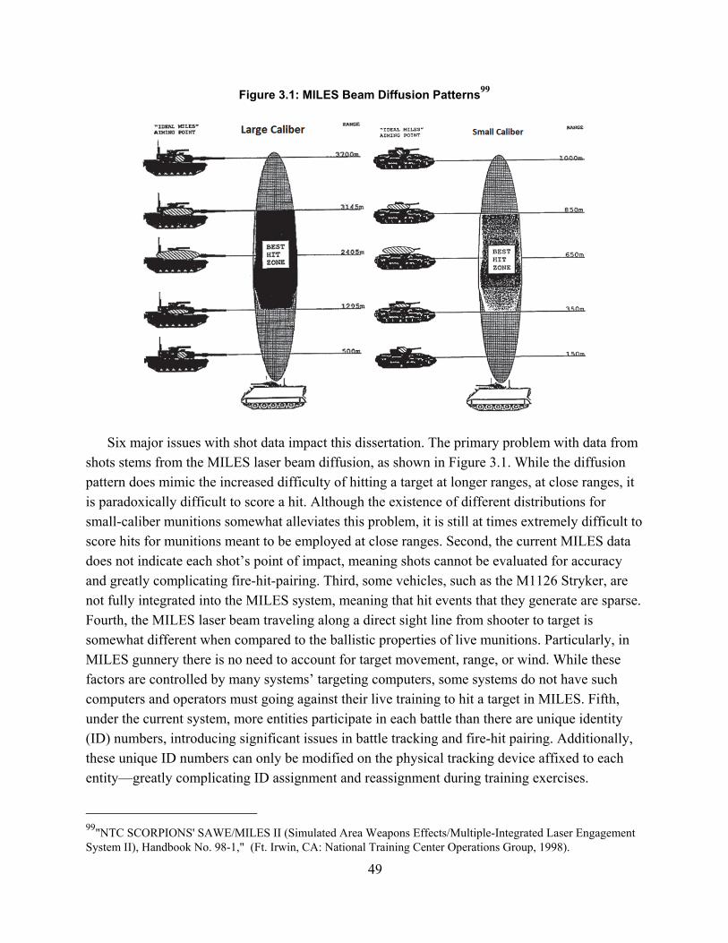
49

Figure 3.1: MILES Beam Diffusion Patterns99

Six major issues with shot data impact this dissertation. The primary problem with data from shots stems from the MILES laser beam diffusion, as shown in Figure 3.1. While the diffusion pattern does mimic the increased difficulty of hitting a target at longer ranges, at close ranges, it is paradoxically difficult to score a hit. Although the existence of different distributions for small-caliber munitions somewhat alleviates this problem, it is still at times extremely difficult to score hits for munitions meant to be employed at close ranges. Second, the current MILES data does not indicate each shot’s point of impact, meaning shots cannot be evaluated for accuracy and greatly complicating fire-hit-pairing. Third, some vehicles, such as the M1126 Stryker, are not fully integrated into the MILES system, meaning that hit events that they generate are sparse. Fourth, the MILES laser beam traveling along a direct sight line from shooter to target is somewhat different when compared to the ballistic properties of live munitions. Particularly, in MILES gunnery there is no need to account for target movement, range, or wind. While these factors are controlled by many systems’ targeting computers, some systems do not have such computers and operators must going against their live training to hit a target in MILES. Fifth, under the current system, more entities participate in each battle than there are unique identity (ID) numbers, introducing significant issues in battle tracking and fire-hit pairing. Additionally, these unique ID numbers can only be modified on the physical tracking device affixed to each entity—greatly complicating ID assignment and reassignment during training exercises.

99"NTC SCORPIONS' SAWE/MILES II (Simulated Area Weapons Effects/Multiple-Integrated Laser Engagement System II), Handbook No. 98-1," (Ft. Irwin, CA: National Training Center Operations Group, 1998).

50

However, the NTC is currently considering system upgrades, which will allow thousands more entities to be tracked by the system. Sixth and finally, there is no indication of which shots were valid combat shots versus which shots that occurred during calibration or by accident outside of battle periods. The lack of such data means that such categories can be at best inferred based on other data attributes or concurrent events.

Direct Fire Hits

The third data type is hit. Each vehicle and tracked soldier is equipped with a number of laser sensors, a GPS receiver, and a radio transmitter. The laser sensors detect MILES laser beams, read the weapon code in any beam detected, and calculate the probability that the detected beam will result in a vehicle/soldier’s destruction. Based on that probability of kill (Pk), one of six outcomes occurs: (1) “near miss,” whereby the fire has no effect on the entity; (2) “hit,” whereby a fire is registered as hitting the entity, but has no effect; (3) “communications kill,” whereby a fire renders the entity unable to communicate with its comrades; (4) “firepower kill,” whereby a fire renders the entity unable to fire; (5) “mobility kill,” whereby a fire renders the entity unable to move; and (6) a “catastrophic kill,” whereby a fire destroys the vehicle (killing all occupants) or kills the soldier.100 Once the outcome of the hit event has been determined by MILES, two subsequent events occur. First, the system transmits a message to the central database, which generates a hit event containing the entity that was hit, what weapon hit it, where the entity was located (based off GPS location), what time the hit occurred, and the weapon that hit it. The system will also usually transmit the ID number of the entity that fired the shot, but because of a small number of ID numbers available, transmission errors, and human error in system initialization, this ID number is not always accurate and must occasionally be discarded. In a separate database event, the entity’s change of state is recorded (from, for example, “healthy” to “catastrophic kill,” based on the outcome of the hit event. If a miss occurs, the weapon type in the database hit event will contain “near miss” as the weapon type and the state will not change. In addition to database events, if the hit resulted in damage or destruction of the vehicle/soldier, audible and visual alarms will indicate a hit and/or kill.101

There are several relevant considerations for hit events. First, fires and hits are not inherently paired in the data transmitted by each MILES laser beam, though the shooter’s identity, when transmitted, greatly aids in pairing accuracy. 102 Second, as discussed with shot events, calibration, accidental shots, or other data errata can artificially generate a number of hit events that are not directly related to combat activity. When calibrating MILES in the first few days of a rotation and after the force-on-force portion of the rotation concludes, many hit events are

100This dissertation does not process entity kill data, because the sensitivity of these would data preclude open publication of this dissertation. 101Chapman, "The Origins and Development of the National Training Center." 102Warrior Training Alliance.

51

generated because of system testing. Hit events may also be created while a vehicle is undergoing maintenance during a rotation. When entities are killed and have their state set to “catastrophic kill,” the system is not supposed to create additional hit events when the entity is subsequently hit; however, because of system errors, this restriction does not always occur. Third, when being hit by a rapid-fire weapon, an entity may generate a number of hit events, with only one corresponding shot event, if that single shot event is recorded as firing multiple rounds. Finally, the auditory and visual signals a hit or killed vehicle emits are at times insufficient to notify the shooting crew that they have scored a hit or kill. At present, the primary means a shooting crew ascertains if they scored a hit is by a small rotating beacon, but a signal can be easily missed if the beacon is obscured or unseen because of the harsh bright desert sunshine. When these signals are missed, shooting crews may mistakenly continue to engage a system that has already been disabled or killed.

Indirect Fire

In addition to direct fire weapons, the Army employs many indirect fire munitions, such as field artillery or mortars, for which a direct laser engagement system would not be effective. For these indirect fires, NTC employs a separate system called Simulation of Area Weapons Effects (SAWE). This system takes as inputs such information from firing vehicles as angle, range, and munitions type and generates a simulated blast, chemical contamination area, or minefield based in the centralized database. Once this simulated area has been populated, the system calculates Pk values for each entity within the area and changes entity states in the database as appropriate. The system then transmits these state changes down to the entities involved, triggering auditory and visual alarms signaling soldiers that they have been hit or killed.103

This data type is excellent from a data completeness point of view, because each shot’s firing position, effective area, central point of impact, and target entities are included with full confidence in each shot event. However, kills generated through indirect fire shots do not generate hit events, so care must be taken to ensure continuity between different data types. Additionally, indirect fire is oftentimes used to create nonlethal effects on the battlefield, such as smoke to obscure friendly movements or illumination to aid reconnaissance. The entities these shots are intended to affect will not be identified in the data as recorded by the database.

Organizational Affiliation

The fourth data type is organizational affiliation. Soldiers and vehicles are assigned in bulk to organizations at the outset of each training rotation. Given that Army organizations follow a hierarchical structure whereby larger organizations command a number of smaller organizations, each organization’s position within the structure and the organization type (i.e., infantry battalion or engineer company) is recorded. These organizations are simplified in preprocessing to include 103 Chapman, The National Training Center Matures: 1985-1993.

52

only the side (Friendly or Hostile), the company, and the parent battalion. As the central unit of analysis in this dissertation is the company, such a simplification will ease processing without losing analytic fidelity. These organizations will also be subject to de-identification in preprocessing, such that each will be represented by a randomized integer number and a unit type description (e.g. support company, armor battalion), rather than a unit name.

While personnel and vehicles may be reassigned to different organizations throughout the rotation, such shuffling is relatively uncommon—especially for the BLUEFOR.104 Additionally, some organizations are marked as down for maintenance, indicating that entities currently assigned to that unit are undergoing maintenance and not directly participating in the battle.

Each of these data types is represented in the Oracle database by a table with component data fields. In its raw form, these data also contain unit, rotational, and date identifying information. This information is removed in preprocessing, thus precluding unit attribution from these data. The list of tables and fields that correspond to these four data types is listed in Table 3.1, along with the data type and any de-identification made for each field.

Table 3.1: List of De-Identified Data Fields

Data Type Table

Field Transformation/Units

Indirect Fire

Fire Mission ID Fire Mission Number

Munitions Quantity Number

Munitions Type Descriptive

Shooter Location_latitude Latitude

Shooter Location_Longitude Longitude

Hit location_Latitude Latitude

Hit location_longitude Longitude

Shooter Entity ID ID number

Time De-identified (time from start of rotation)

Direct Fire

Munitions Quantity Number

Munitions Type Descriptive

Shooter Location_Latitude Latitude

Shooter Location_Longitude Longitude

Shooter Entity ID ID number

Time De-identified (time from start of rotation)

Hit Event

Munitions Quantity Number

Munitions Type Descriptive

Hit Entity Location_latitude Latitude

Hit Entity Longitude

104Personal communication with Warrior Training Alliance.

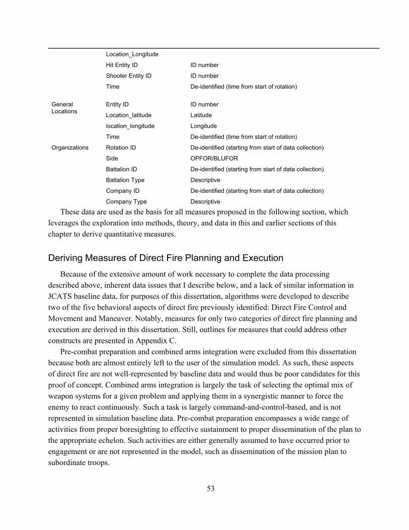
53

Location_Longitude

Hit Entity ID ID number

Shooter Entity ID ID number

Time De-identified (time from start of rotation)

General Locations

Entity ID ID number

Location_latitude Latitude

location_longitude Longitude

Time De-identified (time from start of rotation)

Organizations

Rotation ID De-identified (starting from start of data collection)

Side OPFOR/BLUFOR

Battalion ID De-identified (starting from start of data collection)

Battalion Type Descriptive

Company ID De-identified (starting from start of data collection)

Company Type Descriptive

These data are used as the basis for all measures proposed in the following section, which leverages the exploration into methods, theory, and data in this and earlier sections of this chapter to derive quantitative measures.

Deriving Measures of Direct Fire Planning and Execution

Because of the extensive amount of work necessary to complete the data processing described above, inherent data issues that I describe below, and a lack of similar information in JCATS baseline data, for purposes of this dissertation, algorithms were developed to describe two of the five behavioral aspects of direct fire previously identified: Direct Fire Control and Movement and Maneuver. Notably, measures for only two categories of direct fire planning and execution are derived in this dissertation. Still, outlines for measures that could address other constructs are presented in Appendix C.

Pre-combat preparation and combined arms integration were excluded from this dissertation because both are almost entirely left to the user of the simulation model. As such, these aspects of direct fire are not well-represented by baseline data and would thus be poor candidates for this proof of concept. Combined arms integration is largely the task of selecting the optimal mix of weapon systems for a given problem and applying them in a synergistic manner to force the enemy to react continuously. Such a task is largely command-and-control-based, and is not represented in simulation baseline data. Pre-combat preparation encompasses a wide range of activities from proper boresighting to effective sustainment to proper dissemination of the plan to the appropriate echelon. Such activities are either generally assumed to have occurred prior to engagement or are not represented in the model, such as dissemination of the mission plan to subordinate troops.

54

Direct fire control, which includes such tasks as ensuring distribution of fires among potential targets and massing fires in a critical area, are not modified by any one set of parameters in JCATS, and are thus not tested in this dissertation. Deriving data for sustainment functions (such as maintenance or casualty evacuation) is not viable with the NTC-IS database, nor is it germane to the scenarios that will be modeled in this study.

The scope of measure derivation thus constrained, I derived a total of four measures: Weapon System Probability of Hit, Weapon System Rate of Fire for Direct Fire Control, Unit Dispersion and Unit Speed. These measures are summarized in Table 3.2.

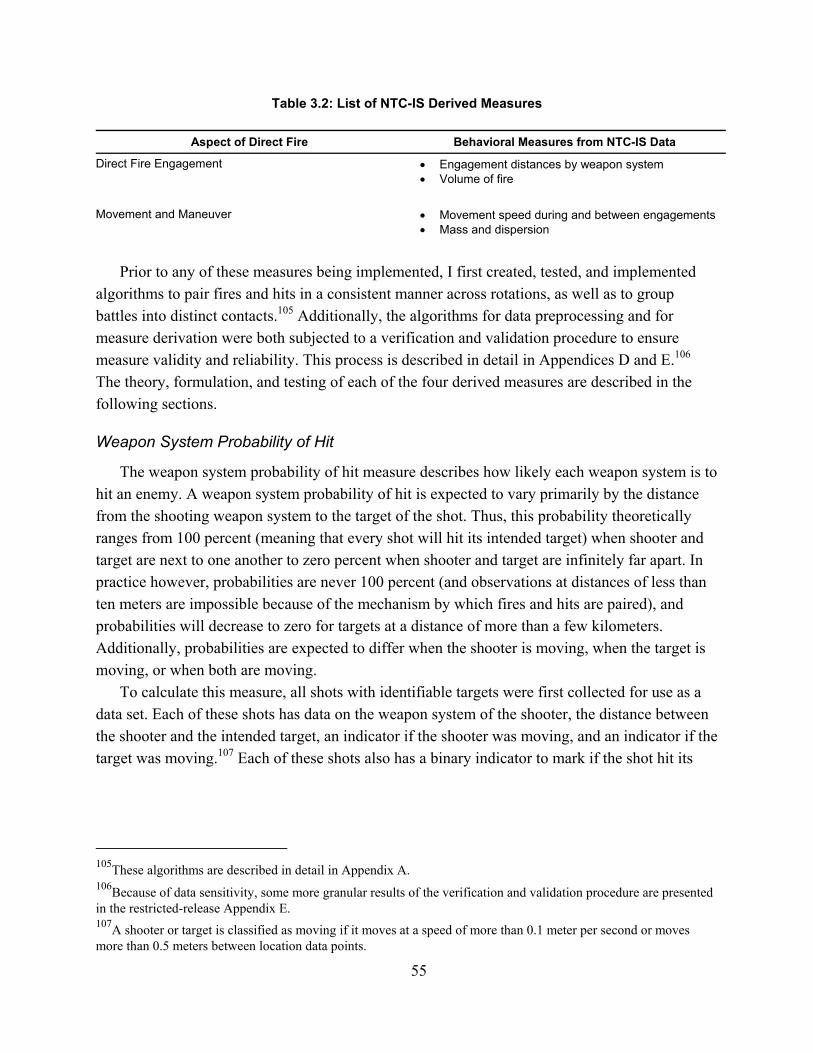
55

Table 3.2: List of NTC-IS Derived Measures

Prior to any of these measures being implemented, I first created, tested, and implemented

algorithms to pair fires and hits in a consistent manner across rotations, as well as to group battles into distinct contacts.105 Additionally, the algorithms for data preprocessing and for measure derivation were both subjected to a verification and validation procedure to ensure measure validity and reliability. This process is described in detail in Appendices D and E.106 The theory, formulation, and testing of each of the four derived measures are described in the following sections.

Weapon System Probability of Hit

The weapon system probability of hit measure describes how likely each weapon system is to hit an enemy. A weapon system probability of hit is expected to vary primarily by the distance from the shooting weapon system to the target of the shot. Thus, this probability theoretically ranges from 100 percent (meaning that every shot will hit its intended target) when shooter and target are next to one another to zero percent when shooter and target are infinitely far apart. In practice however, probabilities are never 100 percent (and observations at distances of less than ten meters are impossible because of the mechanism by which fires and hits are paired), and probabilities will decrease to zero for targets at a distance of more than a few kilometers. Additionally, probabilities are expected to differ when the shooter is moving, when the target is moving, or when both are moving.

To calculate this measure, all shots with identifiable targets were first collected for use as a data set. Each of these shots has data on the weapon system of the shooter, the distance between the shooter and the intended target, an indicator if the shooter was moving, and an indicator if the target was moving.107 Each of these shots also has a binary indicator to mark if the shot hit its

105These algorithms are described in detail in Appendix A. 106Because of data sensitivity, some more granular results of the verification and validation procedure are presented in the restricted-release Appendix E. 107A shooter or target is classified as moving if it moves at a speed of more than 0.1 meter per second or moves more than 0.5 meters between location data points.

Aspect of Direct Fire Behavioral Measures from NTC-IS Data

Direct Fire Engagement Engagement distances by weapon system Volume of fire

Movement and Maneuver Movement speed during and between engagements Mass and dispersion

56

intended target or not. These data are then used to fit a logistic regression model of hit against shooter system type, shooter movement, victim movement, distance, and other controls.108

The coefficients from this regression model were then used to estimate probabilities of hit at 500 meter increments for all weapon systems and for all combinations of shooter and target moving/stationary status.109 As all observed probabilities of hit dropped to zero beyond distances of 5,000 meters, probabilities were only estimated from 0 to 5000 meters.

Weapon System Rate of Fire

The Weapon System Rate of Fire measures how rapidly weapon systems fire their munitions during combat. While each weapon system has a theoretical maximum rate of fire, which is limited by the technology and physical firing mechanism, over a period of many seconds in combat, systems will rarely attain this maximum rate of fire. Instead, battle damage assessment, target reacquisition, maneuver, and other factors will degrade a system’s actual rate of fire.

To assess this rate, this measure first identifies the fastest rate of fire for each entity in each contact that it is involved in over a given time window. In this dissertation, a window duration of 20 seconds is used, because that time is long enough for all weapon systems to fire at least two rounds but still short enough that all shots will likely engage the same target. This measure does not seek to identify initial target acquisition time. These rates thus established at a weapon-system-contact level, I then turn to a Multiple Least Squares regression to precisely estimate rate of fire values for each weapon system and contact type, controlling for a number of potential confounding variables. As rate of fire has a minimum possible value of 0, the natural logarithm of the each weapon-system-contact maximum rate was used as the outcome variable in this analysis. The final model regressed the natural logarithm of a weapon-system-contact maximal rate against the entity type and the contact type, as well as a number of other controls.110 The outputs from this regression model were then used to estimate the rate of fire of each weapon system type at average observed levels of the controlling variables.

Unit Dispersion

Dispersion is the spacing of systems in a unit to protect against enemy fire. Theoretically, a more dispersed unit will survive enemy fire more effectively by both giving the enemy more

108Other controls include the phase of the rotation in which the shot occurred—first third, middle third, or last third— if the shooter was a member of a killer company, the speed of the unit at the time of the shot, and the dispersion of the unit at the time of the shot. 109500 meters was selected as an increment to match as closely as possible the increments of JCATS baseline data. Because the regression coefficients used to predict the final probabilities are continuous, any increment could be used. 110Other controls include the phase of the rotation in which the shot occurred—first third, middle third, or last third—the average accuracy of the weapon system in the contact, an indicator for if the shooter was a member of a killer company (the top 20% of companies when ranked by exchange ratio), the average speed of the firing unit in the contact, and the average dispersion of the firing unit in the contact.

57

targets to engage and by ensuring that not more than one friendly system could be lost to a single enemy shot.111

Different measures for dispersion have been proposed by several researchers attempting to derive measures of combat behavior from NTC data. Proposed measures have included the number of systems within a circle of a given radius centered about a unit’s center of mass,112 the 25th percentile of distance from a unit’s center of mass,113 intra-neighbor distances, and nearest neighbor distances.114 Of these, the two methods requiring the center of mass to be calculated for a unit require the researcher to make a blanket assumption about the distance or proportion of entities to include in the measure, which may not be appropriate for all unit or entity types. Intra-neighbor distances are unacceptably influenced by outliers.115 Nearest-neighbor distance is both robust and matches the doctrinal definition of dispersion, which is based on protection from enemy fire. This dissertation measures dispersion by aggregating the nearest-neighbor distances for all entities in a unit.

This measure is calculated from the NTC-IS at 100-second intervals for each unit in each observed contact. At each sampling interval, the locations of all weapon systems in a given unit are compared and the minimum distance from each system to one of its neighbors is calculated.116 The median of these distances is then used to describe the unit’s dispersion at that sampling interval.

To aggregate this measure by weapon system type, the observed dispersion values are first averaged for each unit over all observed values for that contact. This averaging weights the resultant measure by units and contacts only, without regard for the duration of the contact.117 A Multiple Least Squares linear regression is then used to estimate dispersion values for each unit type and contact type. Because the resultant dispersion values have an absolute minimum at zero meters, the natural logarithm of the observed unit-contact dispersion value is used as the outcome variable in this regression. In the final model, this natural logarithm of dispersion is regressed against unit type, contact type, and a number of controls.118

111If the enemy employs area effect weapons, this distance could be quite large. 112Parker, "Methodology and Analysis of Ground Maneuver Synchronization at the National Training Center." 113Goehring and Sulzen, "Measuring Mass and Speed at the National Training Center." 114Nelson, "Graphical Methods for Depicting Combat Units." 115Ibid. 116This distance is commonly referred to as nearest-neighbor distance. 117Because the goal is to understand how units disperse themselves, the duration of the contact would serve to bias results toward longer contact at the expense of shorter contacts. 118Other controls include the phase of the rotation in which the contact occurred—first third, middle third, or last third—an indicator for if the unit is a killer company, and the average speed of the unit in the contact.

58

Unit Speed

Unit speed is the rate of movement of a unit’s center of mass during physical contact with the enemy. Like Rate of Fire, this speed is limited by the technical specifications of each weapon system. However, also like Rate of Fire, these theoretical maxima are rarely attained—especially during physical contact—because units are actively maneuvering, seeking cover, traversing difficult terrain, firing on the enemy, or otherwise moving at a less-than-maximum rate. Furthermore, because this measure is reported at a unit-level, speed refers to the movement of a unit’s center of mass. Unless all weapon systems in a unit have identical velocities, the aggregate movement speed of that company will be less than that of its members.

Defining the center of mass of a unit centroid of a unit has been the subject of some research in the past. Techniques have ranged from simple averages of entity positions,119 to clustering algorithms,120 to medians of positions along each axis.121 The first of these methods is extremely vulnerable to outliers, which are common in the NTC location database. The second method is time and assumption-intensive, because it requires the researcher to create and tune a clustering algorithm manually. The third is the preferred method, but could be improved on by using the geometric median, the point which has the smallest Euclidian distance to all entities in a unit, rather than the median location along each axis, because this statistic more closely and robustly represents the true center point of a unit.122

To calculate this measure then, the geometric median of all companies in all contacts is calculated at 100-second intervals. The speed for a unit in contact is then defined as the maximal rate of movement of the unit over a defined time window—this dissertation uses 128 seconds as the window duration to cover at least two median locations for each unit.

A unit’s speed in contact thus defined, two methods for aggregating speeds by unit type were investigated. The first employed a regression model in a similar manner to the Unit Dispersion measure—unit speeds were first averaged for each contact,123 then the natural log of the resultant contact speed was taken.124 The natural log of average unit-contact speed was then regressed against entity type and contact type, as well as other controls.125 The resultant coefficients from this model were then used to estimate a unit type’s speed in each contact type.

119Parker, "Methodology and Analysis of Ground Maneuver Synchronization at the National Training Center." 120Ibid. 121Michael S Nelson, "Graphical Methods for Depicting Combat Units" (ibid.1992). 122Hendrik P Lopuhaa and Peter J Rousseeuw, "Breakdown Points of Affine Equivariant Estimators of Multivariate Location and Covariance Matrices," The Annals of Statistics (1991). 123This averaging serves to weight the resultant model by contact, rather than by contact duration. 124Because speed has an absolute lower bound of zero, the log transformation forces the model to estimate coefficients that cannot result in a speed lower than zero. 125Other controls include the phase of the rotation in which the contact occurred—first third, middle third, or last third—an indicator for if the unit is a killer company, and the average dispersion of the unit in the contact.

59

The second method for estimating a unit type’s speed in each contact type is comparatively simple but allows for multiple settings for speed—a feature that made this formulation substantially more useful for creating inputs into the JCATS simulation model. Rather than construct a regression model, which can only estimate a single parameter for each unit type-contact type combination, sufficient data exist to estimate speeds by taking a percentile of the observed data for each unit type and contact type. While this method sacrifices accuracy and precision by removing the ability of the model to control for variation in other variables, it allows for the flexible estimation of as many speed settings as desired. In this dissertation, two such speeds were calculated—one at the 50th percentile of observed speeds, and one at the 75th.126

Discussion

The measures created in this chapter represent a major step forward in filling the data need motivated and identified in Chapters 1 and 2 of this dissertation. These four measures build on previous attempts to measure combat behaviors from NTC data while avoiding the pitfalls of prior studies. In particular, these measures were well-motivated by doctrinal concepts and were developed with an understanding of both the NTC as a data source and the operational environment it represents.

With proper use as data inputs to combat models and simulations, these measures can considerably improve the representativeness of these models of a difficult operational environment such as is represented by the NTC without the need for an expensive operational test or without needing to rely on the limited historical data available. In the next chapter, I examine the use of these measures to improve representativeness in this manner with a scenario developed and tested using the JCATS combat simulation model.

126 There were a great many speeds at or near zero due to a unit being stationary during contact. Using a speed at the 50th percentile controlled well for these extremely low speeds.

60

4. Testing the Difference in JCATS Model Outcomes from Using NTC-based Data

The third portion of this research examines the difference that the NTC-based measures derived in Chapter 3 have on simulation model outcomes. I evaluate this difference by conducting a case study that examines the magnitude and nature of the difference in outputs a simulation model will produce when NTC-IS derived parameters are used in lieu of baseline data. This methodology is in line with best practices for data validation recommended by RAND experts and the Modeling and Simulation Coordination Office. 1

In this chapter, I discuss the model chosen, the inputs to be varied, the outcomes to be examined, the scenario and experimental design used to test the effects. I describe the regression model used to determine effects, and test each outcome variable. From these results, I find a significant difference between runs with NTC inputs compared with baseline inputs. I conclude this chapter by discussing this difference, its generalizability, and its interpretation.

Model Selection

In formulating this case study, I considered a variety of simulation models before ultimately selecting the JCATS model. For this dissertation, I needed a simulation that was well-validated and widely used to maximize the external validity of the dissertation’s findings and ensure generalizability across the DoD. The model also needed to have an extensive set of baseline data that was user-editable to some degree, such that the baseline data may be substituted for data derived from NTC-IS. Finally, the underlying data needed to be accessible and easy enough to manipulate so that a single analyst could modify a number of data fields with minimal set-up and execution time. Three common Army models were considered for this dissertation: One Semi-Automated Forces (OneSAF), Combined Arms Analysis Tool for the 21st Century (COMBATXXI), and (JCATS).

OneSAF is the Army’s internal effort to construct an entity-level tactical combat simulation model that also serves as a connection to virtual training devices, such as the Aviation Combined Arms Tactical Trainer (AVCATT) or CCTT.2 This model has advanced graphics and a large amount of data that is editable by the user and that is strongly influential over behavioral aspects

1Rothenberg et al., "Data Verification, Validation, and Certification (VV&C): Guidelines for Modeling and Simulation."; "Recomended Practices Guide: Data Verification and Validation (V&V) for Legacy Simulations." 2AVCATT is a full-motion helicopter simulation device. CCTT, mentioned previously, is a ground forces virtual reality training system. (see the program office’s websites at http://www.peostri.army.mil/PRODUCTS/AVCATT/ and http://www.peostri.army.mil/PRODUCTS/CCTT/, respectively for more information)

61

of combat. 3 However, it requires a large amount of hardware and manpower to set-up and run—significantly more than was available to complete this dissertation.

COMBATXXI was also examined. This model, developed and maintained by the U.S. Army Training and Doctrine Command Analysis Center (TRAC), is dedicated to analysis, is entirely constructive, and is closed to human intervention once the simulation is under way. TRAC uses this simulation extensively to test and evaluate operational and doctrinal concepts.4 However, the manpower and computing resources required to set-up the model and analyze its results are significant, which precludes its use in this dissertation.

JCATS is an entity-level tactical combat simulation model developed by Lawrence Livermore National Laboratories as an evolution of the older Janus simulation model. Janus was used in many prior simulation studies and has been extensively validated by comparison to historical combat data and to NTC exercise data.5 JCATS, first launched in 1997, adds sea and air capabilities that the earlier model lacked and incorporates a wide range of data that is editable by the user. JCATS is also, according to its capabilities brief, the most widely used combat simulation model in the world, used by over 350 DoD organizations and 30 foreign nations.6 It is designed primarily for training, but is also used for experimentation and analysis and allows for users to adjust thousands of different parameters or construct entirely new weapon systems, thus making this simulation ideal for use in acquisition programs. JCATS can also be installed on a laptop, and pre-scripted scenarios can be rapidly run in batch mode by a single analyst. Thus, this model satisfied all requirements for this research project and was selected for use in this dissertation for this test.

Variable Selection

Here, I discuss the variables used in the model, including the input parameters and the model outcomes.

Input Parameters

To test the difference in outcome between model runs employing baseline inputs compared with those using NTC inputs, four NTC-IS based measures described in Chapter 3 are used in lieu of baseline input parameters that come standard with the JCATS model. Each input

3See http://www.peostri.army.mil/PRODUCTS/ONESAF/ for more information about OneSAF system capabilities. 4"COMBAT XXI," US Army Training and Doctrine Command Analysis Center (TRAC), http://www.trac.army.mil/COMBATXXI.pdf. 5Christenson and Zirkle, "73 Easting Battle Replication--A Janus Combat Simulation.", Lester Ingber, Fujio Hirome, and Michael F. Wehner, "Mathematical Comparison of Combat Computer Models to Exercise Data," Mathematical Computer Modeling 15, no. 1 (1991). 6"Joint Conflict and Tactical Simulation (JCATS) Capabilities Brief," (Livermore, CA: Lawrence Livermore National Laboratories, 2014).

62

parameter required some modifications or transformations to be suitable as an input into the JCATS model; those modifications are described in the following paragraphs.

Weapon System Probability of Hit

Probability of hit is modeled in JCATS with a large number of probability of hit curves, each corresponding to a firing munition type and a target weapon system. Each of these shooter-target pairs has, in turn, 16 different probability of hit curves describing situations in which the shooter is in enfilade or defilade, the target is in enfilade or defilade, the shooter is moving, or the target is moving. Each of these curves manifests itself as a series of points describing a probability at a given distance between shooter and target. In all cases, these probabilities range from 100 percent at a distance of zero from shooter to target to zero percent at distances outside of the given data.

Because information on the enfilade or defilade status of shooter or target is nearly impossible to estimate with the current set of NTC-IS data, the measure for probability of hit derived in this dissertation does not break out results by enfilade or defilade status. Instead, the curves for each of the four possible shooter/target moving/stationary states were averaged together,7 producing a total of four probability of hit curves for each firing weapon system. Using the regression coefficients calculated for the probability of hit measure from the NTC data, estimates for each of these four curves for each firing weapon system were generated. Because of irregularities observed in IFV data (M2s and BMPs), only tank probabilities of hit were used as JCATS input in this dissertation.8 For each curve and each distance from shooter to target, a proportion was calculated by dividing the NTC-based estimate of probability at that distance by the baseline probability at that distance. These proportions were then multiplied by each of the original baseline data curves to obtain the modified probability of hit curve, which was then used as the probability of hit in the JCATS model.

7Because only tanks and IFVs exchanged direct fire in the scenario tested in this dissertation, only tank and IFV target curves were used. Each curve thus became an average of eight total curves. For instance, the “average moving-target-moving-shooter-shooter M1” curve represents the average of the following curves:

moving target-moving shooter- target enfilade-shooter enfilade-target IFV-shooter M1

moving target-moving shooter- target defilade -shooter enfilade-target IFV-shooter M1

moving target-moving shooter- target enfilade-shooter defilade-target IFV-shooter M1

moving target-moving shooter- target defilade-shooter defilade-target IFV-shooter M1

moving target-moving shooter- target enfilade-shooter enfilade-target Tank-shooter M1

moving target-moving shooter- target defilade-shooter enfilade-target Tank-shooter M1

moving target-moving shooter- target enfilade-shooter defilade-target Tank-shooter M1

moving target-moving shooter- target defilade-shooter defilade-target Tank-shooter M1 8See Appendix D for a discussion of this phenomena.

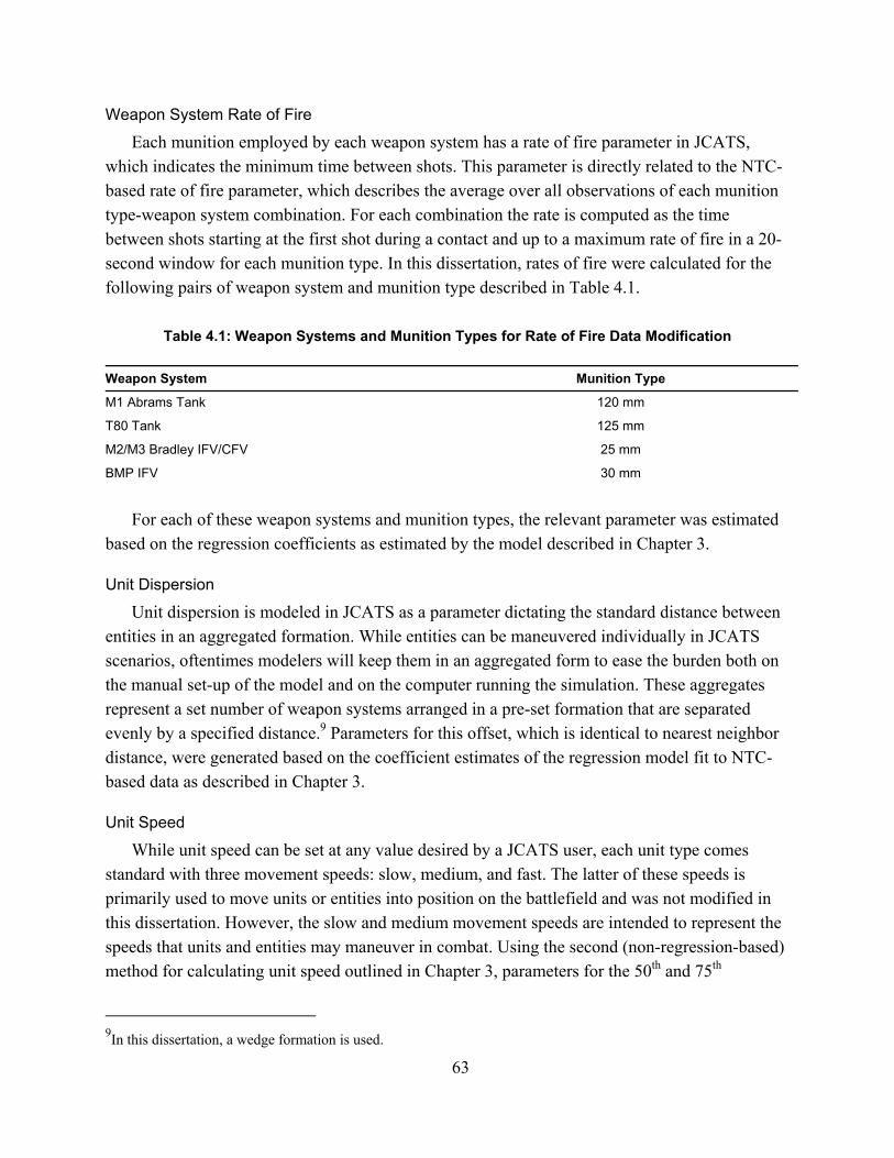
63

Weapon System Rate of Fire

Each munition employed by each weapon system has a rate of fire parameter in JCATS, which indicates the minimum time between shots. This parameter is directly related to the NTC-based rate of fire parameter, which describes the average over all observations of each munition type-weapon system combination. For each combination the rate is computed as the time between shots starting at the first shot during a contact and up to a maximum rate of fire in a 20-second window for each munition type. In this dissertation, rates of fire were calculated for the following pairs of weapon system and munition type described in Table 4.1.

Table 4.1: Weapon Systems and Munition Types for Rate of Fire Data Modification

Weapon System Munition Type

M1 Abrams Tank 120 mm

T80 Tank 125 mm

M2/M3 Bradley IFV/CFV 25 mm

BMP IFV 30 mm

For each of these weapon systems and munition types, the relevant parameter was estimated

based on the regression coefficients as estimated by the model described in Chapter 3.

Unit Dispersion

Unit dispersion is modeled in JCATS as a parameter dictating the standard distance between entities in an aggregated formation. While entities can be maneuvered individually in JCATS scenarios, oftentimes modelers will keep them in an aggregated form to ease the burden both on the manual set-up of the model and on the computer running the simulation. These aggregates represent a set number of weapon systems arranged in a pre-set formation that are separated evenly by a specified distance.9 Parameters for this offset, which is identical to nearest neighbor distance, were generated based on the coefficient estimates of the regression model fit to NTC-based data as described in Chapter 3.

Unit Speed

While unit speed can be set at any value desired by a JCATS user, each unit type comes standard with three movement speeds: slow, medium, and fast. The latter of these speeds is primarily used to move units or entities into position on the battlefield and was not modified in this dissertation. However, the slow and medium movement speeds are intended to represent the speeds that units and entities may maneuver in combat. Using the second (non-regression-based) method for calculating unit speed outlined in Chapter 3, parameters for the 50th and 75th

9In this dissertation, a wedge formation is used.

64

percentile of observed unit speeds were used for these slow and medium speeds, respectively, for each company type.

Model Outcomes

Four combat outcomes are measured from the JCATS model as a result of varying the inputs described in the previous subsection. Model outcomes are commonly accepted combat outcome variables that have been used in prior studies of simulation model effectiveness.10 These measures include: force exchange ratio, drawdown of forces rate for each side, and the total volume of fire on the enemy for each side. For this discussion, the side employing M1 tanks and M2 IFVs is termed the BLUEFOR or “blue”, while the side employing T-80 tanks and BMP IFVs is termed the OPFOR or “red.”

Force Exchange Ratio

The force-exchange ratio is calculated according to the formula:

This ratio defines the proportion of total kills that BLUEFOR caused. The number will be higher for more effective BLUEFOR forces and lower for more effective OPFOR forces.

Drawdown of Forces Rate

The drawdown of forces rate captures the rate of losses of BLUEFOR and OPFOR systems in each of the scenario excursions. This rate gives the average rate of system destruction, in losses per minute, over a one-minute span. This average is weighted by event and reported for each side.11

Volume of Fire

Volume of fire is captured using two separate measures: one for the observed rate of fire, and one for the overall quantity of fire. Each is derived and analyzed separately but is interpreted and discussed here and in the conclusion of this chapter as one measurement construct. The total rate of fire captures the average rate of fire over all systems for each side, expressed in shots per minute. This rate is over a one-minute span and is weighted by shot event, in a manner similar to the drawdown of forces rate measure described in the previous subsection. The second measure

10For an excellent example of such a study that used each of these measures, see John Matsumura et al., "Lightning Over Water: Sharpening America's Light Forces for Rapid Reaction Missions," (Santa Monica, CA: RAND Corporation, 2000). 11 Throughout this section, an event refers to a single shot or hit to or by a weapon system. In this instance an event is a hit on a weapon system that results in that system’s destruction.

65

of volume of fire, the total quantity of fire, is measured by summing all shots taken by each side during the JCATS scenario.

Readers may note that these measures, which here are expressed as outcome measures, are very similar to the rate of fire measure derived from the NTC-IS, which is expressed as a behavioral measure. The difference between these two measures lies in their calculation: the NTC-based input measure calculates the maximal rate of fire over a given time window for each entity in each contact, which it then aggregates at a unit level. The JCATS outcome measure - rate of fire - calculates the average observed rate of fire over a given time window for all shots by a side, weighted by shot event. The former is a measure of maximal system behavior, while the latter is an outcome measuring average unit behavior that results from the JCATS simulation scenario. Furthermore, as the JCATS measure is weighted by shot event, it represents the average intensity of combat in which the side’s shots took place. Because units are expected to mass fires at a key point in the battle to achieve maximal effects on the enemy, a higher rate of fire can be interpreted as a largely positive quality. A higher NTC-based rate of fire has no such interpretation; rather, it simply indicates that the system fires more rapidly, on average. Without knowledge of other system behavior at the time of each shot, it is impossible to make a value judgment on the appropriateness of a high or low individual rate of fire.

Experimental Design

Baseline Scenario Description

To test the sensitivity of the model’s results to changes in mission variables, a baseline scenario and a set of excursions were constructed.

The baseline,12 scenario that this dissertation uses is modeled on a hypothetical NATO conflict in the Baltic states. Specifically, it features an attack by the OPFOR on the BLUEFOR in the area of Jekabpils, Latvia. Because the goal of the modeling effort of this dissertation is to keep as much baseline information in the model as possible for comparison purposes, the order of battle, formation, and system types are all from standard JCATS units. Additionally, all system characteristics remain at the standard baseline levels that JCATS defaults to, unless explicitly adjusted using NTC-based parameters.

BLUEFOR units consist of one combined arms battalion employing two companies of M1A2SEP Abrams tanks, which are armed with a 120mm smoothbore cannon, a .50 caliber machine gun, and a 7.62mm machine gun. In addition to the armor units, BLUEFOR forces include one company of M2A3 Bradley IFVs, which will each be armed with a 25mm cannon, a TOW missile system, and a 7.62mm machine gun. Also included in the BLUEFOR forces are 12 indirect fire assets, 4 Shadow UAS assets, and 4 AH64E Apache Longbow attack helicopters,

12 The baseline scenario is also discussed as the “center” scenario, as it represents central values of each of the three mission variables examined in this study relative to the excursion scenarios.

66

employing the Hellfire Anti-Tank Guided Missile (ATGM) and a 30mm cannon. BLUEFOR begins the battle in defensive positions approximately 6 kilometers outside of the city center.

The OPFOR order of battle consists of one tank battalion primarily employing the T-80, which employs a 125mm main gun, the AT-11 ATGM, and a 7.62mm machine gun. Additionally, OPFOR include one motor-rifle battalion, primarily employing the BMP-2D, which is armed with a 30mm cannon, the AT-5 ATGM, and a 7.62mm machine gun. Finally, OPFOR include 42 indirect fire assets and 9 UAS assets.

The battle consists of a mobile BLUEFOR defense with a focus on the close, direct-fire fight between the two forces. Thus, the scenario begins with both forces located at a distance of 10 kilometers apart (well beyond the maximum range of any direct fire system). Though it is highly likely that in real conflict, forces would have experienced significant attrition before reaching this point in the battle, this scenario ignores such attrition by assuming that the forces that begin the simulation are those that survived earlier attacks.

Once BLUEFOR begins taking losses from OPFOR direct fire, its forces begin to withdraw, using the terrain for cover, into the town of Jekabpils. The BLUEFOR engages in a retrograde defense in depth to slow the OPFOR advance while maintaining combat power as long as possible. In the base scenario, BLUEFOR does not engage in significant spoiling attacks but instead relies on a single engagement area to engage and slow down the OPFOR, before retreating into the city. The scenario ends after 30 minutes of simulation time.

Excursion Scenarios

Because this dissertation proposed a case study methodology for data validation, the selection of scenarios for experimentation was of paramount importance. This study used the six mission variables defined in Army Doctrine Publication (ADP) 3-0 to specify scenario types: Mission, Enemy, Terrain, Troops and support available, Time available and Civil considerations (abbreviated as METT-TC). Since these variables form the basis for mission planning, the tactics employed by the BLUEFOR can be determined by a precise combination of these variables.

Given that the scope of this dissertation is limited to armored and mechanized infantry company-level engagements, three of these factors were held constant throughout the set of scenarios analyzed: civil considerations, because civilian interactions are not well modeled in JCATS; time available, because this factor primarily impacts mission planning timelines, which are assumed to be ideal for this dissertation;13 and troops available, because this dissertation focuses solely on armored companies given time and resource constraints and data reliability. Excluding these factors from consideration is a notable simplification that is applied to the

13Time available does refer to other aspects of time in battle, such as how quickly a given battle should progress, or at which point friendly units need to synchronize with other echelons. However, given the constraints of the simulation model, these factors could not be well modeled. Also, time is an explicit component of some of the measures, such as, rate of fire. Future research efforts may include investigations into the effects of time constraints on model outcomes.

67

potential space of scenarios, the effects of which will be discussed in the conclusion of this chapter.

Thus, the three variables of Mission, Enemy and Terrain form the expected variability between simulation scenarios that this dissertation seeks to generalize to. The three variables thus compose a three-dimensional space which can be sampled to identify the range of operations that adjusted data in the simulation model may affect.

This dissertation creates scenario excursions at points in this three-dimensional space defined by these mission variables, then tests those scenarios using both NTC and JCATS baseline inputs to determine what differences in the outcome variables examined may arise. Though there are an infinite number of possible cases in the three-dimensional Mission, Enemy and Terrain space, each scenario takes considerable time and effort to plan, develop, and test. Given time and resources available, any increase in the number of scenarios to develop would inevitably result in a reduction in scenario quality. I thus used the parsimonious Plackett-Burman experimental design to efficiently sample the space with four corner cases and one center point.1415 The center point helps to control and test for possible curvature in mission variable effects, though it will not allow for curvature testing in the effect of NTC data on outcomes or the effect of side on outcomes. This design is depicted in graphical form in Figure 4.1, with green dots indicating the configurations of the five scenarios that were constructed and tested.

14R. L. Plackett and J.P. Burman, "The Design of Optimum Multifactorial Experiments," Biometrika 33, no. 4 (1946). 15The center point is not included in most Plackett-Burman designs but is added in this case to enable the testing for curvature of effects and to provide an additional degree of freedom for sampling confidence.

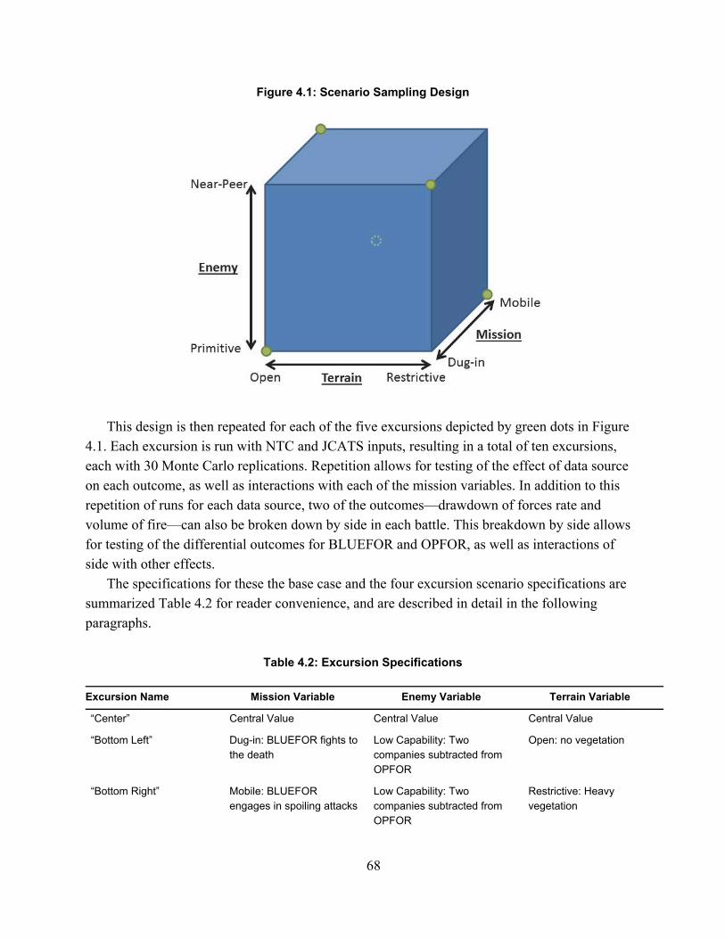
68

Figure 4.1: Scenario Sampling Design

This design is then repeated for each of the five excursions depicted by green dots in Figure

4.1. Each excursion is run with NTC and JCATS inputs, resulting in a total of ten excursions, each with 30 Monte Carlo replications. Repetition allows for testing of the effect of data source on each outcome, as well as interactions with each of the mission variables. In addition to this repetition of runs for each data source, two of the outcomes—drawdown of forces rate and volume of fire—can also be broken down by side in each battle. This breakdown by side allows for testing of the differential outcomes for BLUEFOR and OPFOR, as well as interactions of side with other effects.

The specifications for these the base case and the four excursion scenario specifications are summarized Table 4.2 for reader convenience, and are described in detail in the following paragraphs.

Table 4.2: Excursion Specifications

Excursion Name Mission Variable Enemy Variable Terrain Variable

“Center” Central Value Central Value Central Value

“Bottom Left” Dug-in: BLUEFOR fights to the death

Low Capability: Two companies subtracted from OPFOR

Open: no vegetation

“Bottom Right” Mobile: BLUEFOR engages in spoiling attacks

Low Capability: Two companies subtracted from OPFOR

Restrictive: Heavy vegetation

69

“Top Left” Mobile: BLUEFOR engages in spoiling attacks

High Capability: Two companies added to OPFOR

Open: no vegetation

“Top Right” Dug-in: BLUEFOR fights to the death

High Capability: Two companies added to OPFOR

Restrictive: Heavy vegetation

Bottom Left Excursion

In this scenario, BLUEFOR does not move from its initial positions, instead fighting to the death. OPFOR strength is also reduced by one T80 company and one BMP company (from the front and rear of OPFOR’s starting formation, respectively) compared with the center scenario. Finally, this scenario simulates open terrain by raising each vehicle’s sensor height to 150% of normal.

Bottom Right Excursion

In this scenario, BLUEFOR engages in a more active defense, engaging in a small spoiling attack as OPFOR approaches. This spoiling attack involves the BLUEFOR’s “lower” tank company emplacing itself about a kilometer to the East (in a position where OPFOR cannot observe them until they are quite close). Once the remainder of BLUEFOR begins engaging OPFOR, this company launches a small attack on OPFOR’s flank to cover the retreat of their compatriots. After briefly engaging, this company begins to retreat along with its compatriots. Additionally, the more southerly pair of AH64s is emplaced about three kilometers to the east of their final location to cover the retreat of all three companies. Two companies are subtracted from the OPFOR, as in the Bottom Left scenario. This scenario also simulates restrictive terrain by reducing each vehicle’s sensor height to 66.7 percent of normal.

Top Left Excursion

In this scenario, BLUEFOR engages in spoiling attacks as in the Bottom Right scenario. OPFOR strength is increased by adding two companies (one T80 and one BMP) to the front and rear of the starting force positions, respectively. This scenario simulates open terrain by raising each vehicle’s sensor height to 150 percent of normal.

Top Right Excursion

In this scenario, BLUEFOR fights to the death as in the Bottom Left scenario. OPFOR is strengthened with two additional companies as in the Top Right scenario. Restrictive terrain is simulated by reducing sensor height to 66.7 percent of normal.

70

Effect Aliasing

There were two experimental designs employed for all analyses. The first design applies to analyses when an input could not be differentiated for both sides (e.g., force exchange ratio): this design is listed as “Design A: Repeated by Input Source” in Table 4.3. The second experimental design was applied when the input sources can be broken down by side, will be referred to as Design B. The specific effects to be tested for are summarized in Table 4.3.

Table 4.3: Summary of Experimental Design Effect Estimation

Design A: Repeated by Input Source Design B: Repeated by Data Source and Side

Applicable Outcomes Exchange Ratio Drawdown of Forces Rate Volume of Fire—Rate Volume of Fire--Quantity

First-Order Effects Data Source Mission Enemy Terrain

Data Source Side Mission Enemy Terrain

Second-Order Effects Mission & Data Source Enemy & Data Source Terrain & Data Source

Side & Data Source Mission & Data Source Enemy & Data Source Terrain & Data Source Mission & Side Enemy & Side Terrain & Side

Third-Order Effects Mission & Side & Data Source Enemy & Side & Data Source Terrain & Side & Data Source

Although these designs are efficient, requiring few specifications to estimate the desired

effects, it comes with a major cost in the form of aliased effects. Each lower-order effect examined in this dissertation is aliased with a higher-order interaction term.16 It is impossible to determine without doubt whether the observed effect is the result of the lower-order primary effect or its higher-order aliased effect. This dissertation assumes, in line with the experimental design literature, that these higher-order effects have comparatively little impact on outcome and thus that the observed coefficient on each effect is primarily the result of the lower-order effect. While this research assumes that the potentially aliasing higher-order effects are greatly outweighed by the corresponding lower-order effects, potential aliasing will be mentioned and incorporated into analysis of model results. The aliasing structure for each design is listed in Tables 4.4 and 4.5, for Design A and B, respectively.

16 For instance, a first-order effect may be aliased with a second or third-order effect, a second order effect may be aliased with a third or fourth-order effect, and so on, as indicated in tables 4.3 and 4.4

71

Table 4.4: Aliasing Structure for Design A

Order of Primary Effect Low-Order Primary Effect High-Order Aliased Effect

First Order Data Source Mission Enemy Terrain

= = = =

Enemy & Mission & Terrain Enemy & Terrain Mission & Terrain Enemy & Mission

Second Order Mission & Data Source Enemy & Data Source Terrain & Data Source

= = =

Enemy & Terrain & Data Source Mission & Terrain & Data Source Enemy & Mission & Data Source

Table 4.5: Aliasing Structure for Design B

Order of Primary Effect Low-Order Primary Effect High-Order Aliased Effect

First Order Data Source Side

Enemy Mission Terrain

= = = = =

Mission & Enemy & Terrain & Data Source Mission & Enemy & Terrain & Side Mission & Terrain Enemy & Terrain Mission & Enemy

Second Order Side & Data Source

Mission & Data Source Enemy & Data Source Terrain & Data Source

Mission & Side Enemy & Side Terrain & Side

= = = = = = =

Mission & Enemy & Terrain & Side & Data Source Enemy & Terrain & Data Source Mission & Terrain & Data Source Mission & Enemy & Data Source Enemy & Terrain & Side Mission & Terrain & Side Mission & Enemy & Side

Third Order Mission & Side & Data Source Enemy & Side & Data Source Terrain & Side & Data Source

= = =

Enemy & Terrain & Side & Data Source Mission & Terrain & Side & Data Source Mission & Enemy & Side & Data Source

Factor Coding and Sample Size

For analytical purposes, factors are included in a regression model coded as a -1, 1, or 0 value, indicating a high, low, or central value for that factor, respectively. Additionally, data source is coded a 1 or a 0, with 0 indicating JCATS baseline data and 1 indicating NTC-based data. Side is coded 1 or 0, with a 0 indicating the BLUEFOR and a 1 indicating the OPFOR. The settings are summarized for the mission variables in Table 4.6 and are described in greater detail in the following section.17

Table 4.6: Summary of Mission Variable Effects on JCATS Excursions

Excursion Name

Mission Enemy Terrain

17The full experimental design matrix for designs A and B are included in Appendix F.

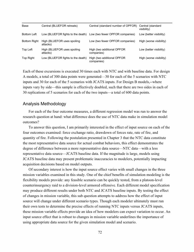
72

Base Central (BLUEFOR retreats) Central (standard number of OPFOR) Central (standard visibility)

Bottom Left Low (BLUEFOR fights to the death) Low (two fewer OPFOR companies) Low (better visibility)

Bottom Right High (BLUEFOR uses spoiling attacks)

Low (two fewer OPFOR companies) High (worse visibility)

Top Left High (BLUEFOR uses spoiling attacks)

High (two additional OPFOR companies)

Low (better visibility)

Top Right Low (BLUEFOR fights to the death) High (two additional OPFOR companies)

High (worse visibility)

Each of these excursions is executed 30 times each with NTC and with baseline data. For design A models, a total of 300 data points were generated—30 for each of the 5 scenarios with NTC inputs and 30 for each of the 5 scenarios with JCATS inputs. For Design B models,--where inputs vary by side—this sample is effectively doubled, such that there are two sides in each of 30 replications of 5 scenarios for each of the two inputs—a total of 600 data points.

Analysis Methodology

For each of the four outcome measures, a different regression model was run to answer the research question at hand: what difference does the use of NTC data make in simulation model outcomes?

To answer this question, I am primarily interested in the effect of input source on each of the four outcomes examined: force exchange ratio, drawdown of forces rate, rate of fire, and quantity of fire. Following the postulation presented in Chapter 3 that the NTC data constitute the most representative data source for actual combat behaviors, this effect demonstrates the degree of difference between a more representative data source—NTC data—with a less representative data source—JCATS baseline data. If the magnitude is large, models using JCATS baseline data may present problematic inaccuracies to modelers, potentially impacting acquisition decisions based on model outputs.

Of secondary interest is how the input source effect varies with small changes in the three mission variables examined in this study. One of the chief benefits of simulation modeling is the flexibility models provide: any feasible scenario can be quickly tested, from a platoon-level counterinsurgency raid to a division-level armored offensive. Each different model specification may produce different results under both NTC and JCATS baseline inputs. By testing the effect of changes in mission variable, this sub question attempts to address how the effect of input source will change under different scenario types. Though each modeler ultimately must run their own tests to determine the precise effects of running NTC inputs versus JCATS inputs, these mission variable effects provide an idea of how modelers can expect variation to occur. An input source effect that is robust to changes in mission variable underlines the importance of using appropriate data source for the given simulation model and scenario.

73

Effect sizes are estimated using a Multiple Least Squares (MLS) regression, with the outcomes for each variable regressed against the factor settings corresponding to each sample. Standard errors are computed according to a bootstrap procedure with 1,000 replications.

In addition to estimates for coefficients on variables for each effect and combination of higher-order effects,18 all four models include an estimate for a constant term and a curvature term. The constant term is standard in multiple linear regression and represents a scenario with “0” values for each of input source and the three mission variables, which is the specification for the baseline/JCATS input scenario. All coefficients collectively add to or subtract from this constant value in each regression model result.

The curvature term is the coefficient on a variable indicating the center scenario and, if significant, indicates some degree of non-linearity of effect between the high and low settings of any given variable. Said differently, the coefficient on the curvature term indicates the degree to which the outcome in the center-point scenario is higher or lower than would otherwise be expected given the independent variables in this model. Given the qualitative nature of the mission variables and their specification, some degree of non-linearity of effects sizes is expected. A significant curvature term further emphasizes that any extrapolation of these coefficients to other values of mission variable, or to other scenarios, will almost certainly be biased to some degree. Rather, trends and qualitative conclusions can be drawn from this research, instead of specific effect magnitudes.

Model Results

Force Exchange Ratio

The force exchange ratio measures the proportion of total hits in each simulation run that were scored by the BLUEFOR. The average numbers of OPFOR and BLUEFOR kills over all 30 replications of each scenario are displayed in Table 4.7. The far right column contains the exchange ratio average across all repetitions for each scenario excursion. To interpret the table, consider the first row of results. The “Base” scenario represents middle values of each of the three mission variables, and the baseline input source indicates JCATS inputs, rather than NTC. Under this specification, the OPFOR kills 15.7 Blue weapon systems and the BLUEFOR kills 74 Red weapon systems. These losses equate to an exchange ratio of 0.83. One can also think of this ratio as BLUEFOR killing approximately 4.9 Red weapon systems for every Blue system lost.

Table 4.7: Summary of Observed Force Exchange Ratios

Scenario Name Input source OPFOR Kills BLUEFOR Kills Exchange Ratio

18 Second and third order

74

Base Baseline 15.733 74.167 0.830

Bottom Left (dug-in Mission/low Enemy/open Terrain)

Baseline 8.067 71.900 0.901

Bottom Right (mobile Mission/low Enemy/rest. Terrain)

Baseline 8.867 49.867 0.854

Top Left (mobile Mission/high Enemy/open Terrain)

Baseline 15.500 83.533 0.847

Top Right (dug-in Mission/high Enemy/rest. Terrain)

Baseline 12.600 133.933 0.916

Base NTC 22.933 75.067 0.764

Bottom Left (dug-in Mission/low Enemy/open Terrain)

NTC 13.433 65.700 0.838

Bottom Right (mobile Mission/low Enemy/rest. Terrain)

NTC 10.100 48.933 0.831

Top Left (mobile Mission/high Enemy/open Terrain)

NTC 28.733 70.833 0.709

Top Right (dug-in Mission/high Enemy/rest. Terrain)

NTC 29.500 96.867 0.758

From these results, one can see that both NTC and JCATS inputs result in ordinally logical

results—BLUEFOR far outmatches OPFOR in each scenario, but OPFOR performs better with more forces—but there are substantial differences in magnitude that indicate significant input source effects. Based on the averages across scenario excursions, there is a uniform reduction in exchange ratio—meaning the outcome was less favorable to BLUEFOR—in scenarios using NTC data compared with those using baseline data. Specifically, the exchange ratios for excursions with JCATS inputs ranged from 0.83 to 0.92 and the range of exchange ratios with NTC inputs ranged from 0.71 to 0.84. As described in the experimental design section of this dissertation, a Multiple Least Squares regression model was estimated to test the magnitude of these differences and to determine if these observed differences between input sources were statistically significant. Because this outcome cannot be broken down by side for each engagement,19 the effect is modeled according to Design A, the exact experimental design for which is presented in Appendix F along with the regression equation and model diagnostics.

The resulting model has an R-squared value of 0.3710, 291 degrees of freedom and an overall chi-squared statistic of 276.111 (p value <0.0001).The coefficients on each effect are presented in Table 4.8. Those coefficients significant at the 95% level or greater are discussed in the following paragraphs.

19The exchange ratio from the perspective of the OPFOR is simply the inverse of the ratio used in this analysis

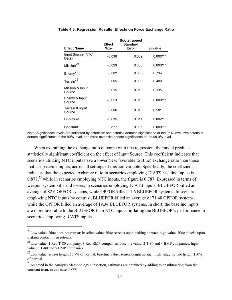
75

Table 4.8: Regression Results: Effects on Force Exchange Ratio

Effect Name Effect Size

Bootstrapped Standard

Error p-value

Input Source (NTC Data)

-0.090 0.009 0.000***

Mission20

-0.029 0.006 0.000***

Enemy21

0.002 0.006 0.734***

Terrain22

0.005 0.006 0.400***

Mission & Input Source

0.015 0.010 0.135***

Enemy & Input Source

-0.053 0.010 0.000***

Terrain & Input Source

0.006 0.010 0.581***

Curvature -0.035 0.011 0.002***

Constant 0.877 0.006 0.000***

Note: Significance levels are indicated by asterisks: one asterisk denotes significance at the 95% level, two asterisks denote significance at the 99% level, and three asterisks denote significance at the 99.9% level.

When examining the exchange ratio outcome with this regression, the model predicts a

statistically significant coefficient on the effect of Input Source. This coefficient indicates that scenarios utilizing NTC inputs have a lower (less favorable to Blue) exchange ratio than those that use baseline inputs, across all settings of mission variable. Specifically, the coefficient indicates that the expected exchange ratio in scenarios employing JCATS baseline inputs is 0.877,23 while in scenarios employing NTC inputs, the figure is 0.787. Expressed in terms of weapon system kills and losses, in scenarios employing JCATS inputs, BLUEFOR killed an average of 82.6 OPFOR systems, while OPFOR killed 11.6 BLUEFOR systems. In scenarios employing NTC inputs by contrast, BLUEFOR killed an average of 71.48 OPFOR systems, while the OPFOR killed an average of 19.34 BLUEFOR systems. In short, the baseline inputs are more favorable to the BLUEFOR than NTC inputs, inflating the BLUEFOR’s performance in scenarios employing JCATS inputs.

20Low value: Blue does not retreat; baseline value: Blue retreats upon making contact; high value: Blue attacks upon making contact, then retreats. 21Low value: 1 Red T-80 company, 3 Red BMP companies; baseline value: 2 T-80 and 4 BMP companies; high value: 3 T-80 and 5 BMP companies. 22Low value: sensor height 66.7% of normal, baseline value: sensor height normal, high value: sensor height 150% of normal. 23As noted in the Analysis Methodology subsection, estimates are obtained by adding to or subtracting from the constant term, in this case 0.877)

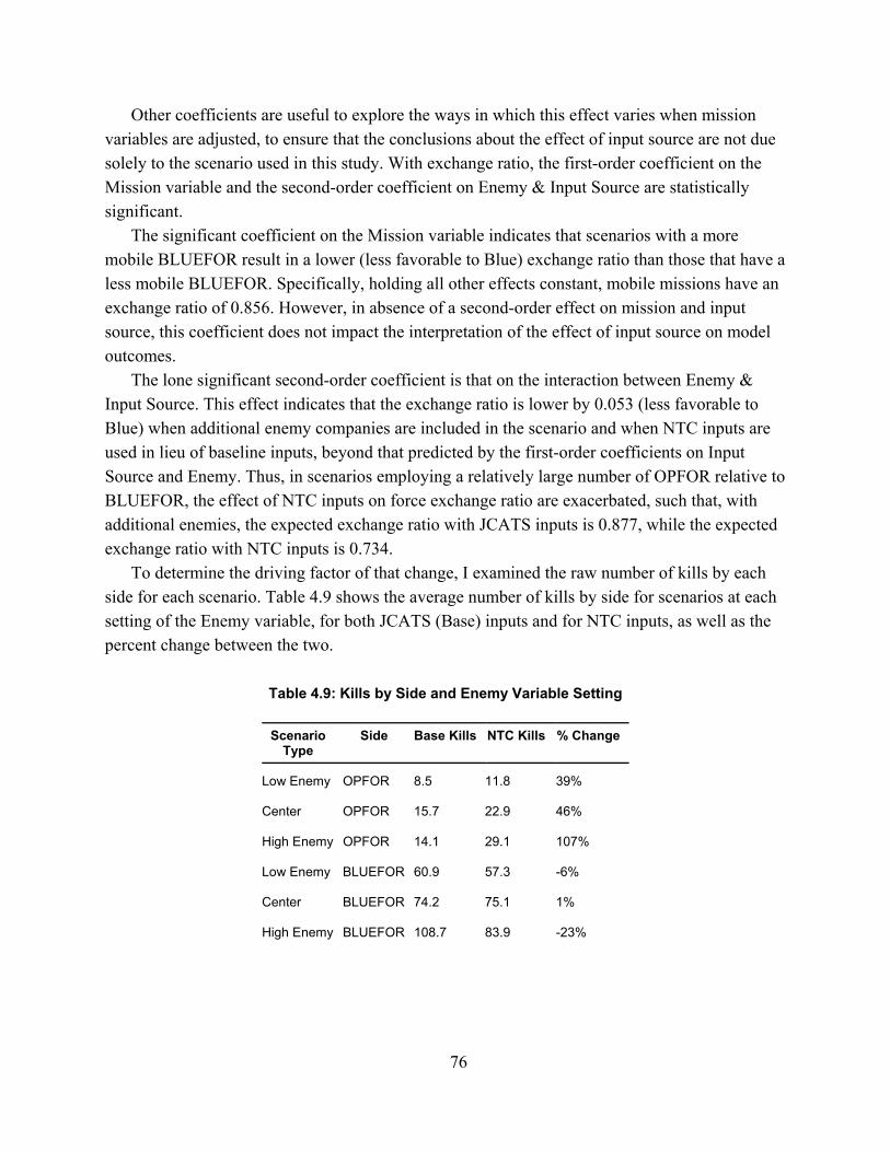
76

Other coefficients are useful to explore the ways in which this effect varies when mission variables are adjusted, to ensure that the conclusions about the effect of input source are not due solely to the scenario used in this study. With exchange ratio, the first-order coefficient on the Mission variable and the second-order coefficient on Enemy & Input Source are statistically significant.

The significant coefficient on the Mission variable indicates that scenarios with a more mobile BLUEFOR result in a lower (less favorable to Blue) exchange ratio than those that have a less mobile BLUEFOR. Specifically, holding all other effects constant, mobile missions have an exchange ratio of 0.856. However, in absence of a second-order effect on mission and input source, this coefficient does not impact the interpretation of the effect of input source on model outcomes.

The lone significant second-order coefficient is that on the interaction between Enemy & Input Source. This effect indicates that the exchange ratio is lower by 0.053 (less favorable to Blue) when additional enemy companies are included in the scenario and when NTC inputs are used in lieu of baseline inputs, beyond that predicted by the first-order coefficients on Input Source and Enemy. Thus, in scenarios employing a relatively large number of OPFOR relative to BLUEFOR, the effect of NTC inputs on force exchange ratio are exacerbated, such that, with additional enemies, the expected exchange ratio with JCATS inputs is 0.877, while the expected exchange ratio with NTC inputs is 0.734.

To determine the driving factor of that change, I examined the raw number of kills by each side for each scenario. Table 4.9 shows the average number of kills by side for scenarios at each setting of the Enemy variable, for both JCATS (Base) inputs and for NTC inputs, as well as the percent change between the two.

Table 4.9: Kills by Side and Enemy Variable Setting

Scenario Type

Side Base Kills NTC Kills % Change

Low Enemy OPFOR 8.5 11.8 39%

Center OPFOR 15.7 22.9 46%

High Enemy OPFOR 14.1 29.1 107%

Low Enemy BLUEFOR 60.9 57.3 -6%

Center BLUEFOR 74.2 75.1 1%

High Enemy BLUEFOR 108.7 83.9 -23%

77

From this table, two points are immediately clear. The first is that, in nearly all cases, OPFOR kills more and BLUEFOR kills less with NTC inputs compared with JCATS inputs.24 Additionally, the High Enemy scenarios have a percent change between kills with JCATS and NTC inputs substantially different from the other scenarios. This difference suggests that the driving data points behind the Enemy & Input Source term are the High Enemy scenarios, which cause significantly more OPFOR kills and BLUEFOR losses. Thus, as comparable threats grow more numerous and capable in simulation models, the effect of using the appropriate input source significantly increases.

Finally, the curvature term in this model is significant, indicating some degree of non-linearity of effect between the high and low settings for at least one variable. This non-linearity emphasizes the need for future researchers to conduct their own tests for effect sizes using their own scenarios, rather than taking the given coefficients as-is.

Drawdown of Forces Rate

The drawdown of forces rate measures the rate at which weapon systems are destroyed for each side. The average loss rates of OPFOR and BLUEFOR weapon systems over all 30 replications of each scenario are displayed in Table 4.10. Loss rates are expressed in terms of losses per minute. Consider the first row of the table, displaying data from the “base” scenario with JCATS inputs. The base scenario specifies middle values for each of the three middle values and JCATS inputs, rather than NTC. Under this specification, the average OPFOR loss rate is 19.546 weapon systems (of any type) per minute, while the BLUEFOR rate is 3.779 systems per minute.

Table 4.10: Observed Values of Drawdown of Forces Rate

Scenario Name Input Source OPFOR Loss Rate BLUEFOR Loss Rate

Base Baseline 19.546 3.779

Bottom Left (dug-in Mission/low Enemy/open Terrain)

Baseline 14.770 2.486

Bottom Right (mobile Mission/low Enemy/rest. Terrain)

Baseline 13.456 2.200

Top Left (mobile Mission/high Enemy/open Terrain)

Baseline 21.096 3.919

Top Right (dug-in Mission/high Enemy/rest. Terrain)

Baseline 22.387 3.678

Base NTC 15.646 5.998

24 In the Center –BLUEFOR case, the difference is minimal

78

Bottom Left (dug-in Mission/low Enemy/open Terrain)

NTC 13.997 3.719

Bottom Right (mobile Mission/low Enemy/rest. Terrain)

NTC 12.077 2.680

Top Left (mobile Mission/high Enemy/open Terrain)

NTC 14.467 6.467

Top Right (dug-in Mission/high Enemy/rest. Terrain)

NTC 13.603 6.950

As with the force exchange ratio outcome, these results show broadly similar outcomes under

both NTC and JCATS inputs—BLUEFOR loss rates are lower than OPFOR rates, but increase when they face more enemies. Again however, there exist substantial differences in magnitude under the two inputs sources, revealing important input source effects. Under every scenario specification, the BLUEFOR loss rate increases and the OPFOR loss rate decreases in scenarios employing NTC inputs, compared with those using JCATS inputs. OPFOR loss rates under JCATS inputs ranged from 13.456 to 22.387 systems per minute, while under NTC inputs they ranged from 12.077 to 15.646. BLUEFOR loss rates under JCATS inputs ranged from 2.200 to 3.919 systems per minute while under NTC inputs they ranged from 2.680 to 6.950. To identify the magnitude and significance of this effect, as well as other variations that result from changes in mission variable and side, I further analyzed these results with a Multiple Least Squares regression. Because this outcome can be broken down by side for each engagement, this effect is modeled according to Design B, the exact experimental design for which is presented in Appendix F along with the regression equation and model diagnostics.

The resulting model has an R-squared value of 0.8862 and an overall chi-squared statistic of 5424.48 (P value <0.0001). The coefficients on each effect are presented in Table 4.11; those significant at the 95% level or higher are discussed in more detail in the following paragraphs.

Table 4.11: Regression Results – Effects on Drawdown of Forces Rate

Effect Name Effect Size Bootstrapped Standard Error P-value

Input Source (NTC Inputs) 1.950 0.189 0.000***

Side (OPFOR) 15.039 0.283 0.000***

Mission25

-0.011 0.128 0.932***

Enemy26

0.728 0.128 0.000***

Terrain27

-0.132 0.128 0.304***

25Low value: Blue does not retreat; baseline value: Blue retreats upon making contact; high value: Blue attacks upon making contact, then retreats. 26Low value: 1 Red T-80 company, 3 Red BMP companies; baseline value: 2 T-80 and 4 BMP companies; high value: 3 T-80 and 5 BMP companies.

79

Side & Input Source -6.243 0.387 0.000***

Mission & Input Source -0.369 0.207 0.073***

Enemy & Input Source 1.027 0.207 0.000***

Terrain & Input Source -0.007 0.207 0.971***

Mission & Side -0.640 0.326 0.051***

Enemy & Side 3.087 0.326 0.000***

Terrain & Side 0.126 0.326 0.708***

Mission & Side & Input Source 0.757 0.436 0.082***

Enemy & Side & Input Source -4.342 0.436 0.000***

Terrain & Side & Input Source -0.683 0.436 0.121***

Curvature 1.370 0.235 0.000***

Constant 2.938 0.127 0.000***

Note: Significance levels are indicated by asterisks: one asterisk denotes significance at the 95% level, two asterisks denote significance at the 99% level, and three asterisks denote significance at the 99.9% level.

When examining the drawdown of forces rate outcome with this regression, the model

predicts a statistically significant coefficient on the effect of Input Source, as well as on side and the interaction between Input Source & Side. The significance of all three of these coefficients indicates all four possible drawdown of forces rates are significantly distinct. Specifically, this model estimates that the drawdown of forces rate for OPFOR units under JCATS baseline inputs is 17.977 and under NTC inputs is 13.683.28 For BLUEFOR units, the model estimates a drawdown rate of 2.938 under JCATS inputs and 4.888 under NTC inputs. These results indicate that when NTC input is used instead of JCATS baseline input the battle proceeds less favorably for BLUEFOR in that they lose combat power much more quickly, while their opponents maintain their combat power for longer. These results are summarized, along with percentage changes in Table 4.12.

Table 4.12: Model Estimates of Drawdown of Force Rate by Side and Input Source

Side Base Inputs NTC Inputs % Change

BLUEFOR 2.938 4.889 66.4%

OPFOR 17.977 13.684 -23.9%

To explore the ways in which the effect of input source varies when mission variables are

adjusted, statistically significant coefficients on interaction terms of mission variables and input

27Low value: sensor height 66.7% of normal, baseline value: sensor height normal, high value: sensor height 150% of normal. 28 As noted in the Analysis Methodology subsection, estimates are obtained by adding to or subtracting from the constant term, in this case 2.938 losses per minute)

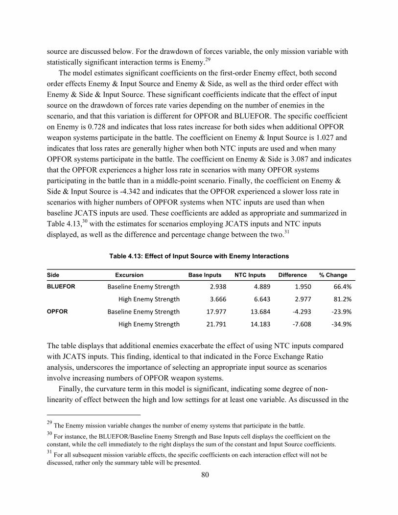
80

source are discussed below. For the drawdown of forces variable, the only mission variable with statistically significant interaction terms is Enemy.29

The model estimates significant coefficients on the first-order Enemy effect, both second order effects Enemy & Input Source and Enemy & Side, as well as the third order effect with Enemy & Side & Input Source. These significant coefficients indicate that the effect of input source on the drawdown of forces rate varies depending on the number of enemies in the scenario, and that this variation is different for OPFOR and BLUEFOR. The specific coefficient on Enemy is 0.728 and indicates that loss rates increase for both sides when additional OPFOR weapon systems participate in the battle. The coefficient on Enemy & Input Source is 1.027 and indicates that loss rates are generally higher when both NTC inputs are used and when many OPFOR systems participate in the battle. The coefficient on Enemy & Side is 3.087 and indicates that the OPFOR experiences a higher loss rate in scenarios with many OPFOR systems participating in the battle than in a middle-point scenario. Finally, the coefficient on Enemy & Side & Input Source is -4.342 and indicates that the OPFOR experienced a slower loss rate in scenarios with higher numbers of OPFOR systems when NTC inputs are used than when baseline JCATS inputs are used. These coefficients are added as appropriate and summarized in Table 4.13,30 with the estimates for scenarios employing JCATS inputs and NTC inputs displayed, as well as the difference and percentage change between the two.31

Table 4.13: Effect of Input Source with Enemy Interactions

Side Excursion Base Inputs NTC Inputs Difference % Change

BLUEFOR Baseline Enemy Strength 2.938 4.889 1.950 66.4%

High Enemy Strength 3.666 6.643 2.977 81.2%

OPFOR Baseline Enemy Strength 17.977 13.684 ‐4.293 ‐23.9%

High Enemy Strength 21.791 14.183 ‐7.608 ‐34.9%

The table displays that additional enemies exacerbate the effect of using NTC inputs compared with JCATS inputs. This finding, identical to that indicated in the Force Exchange Ratio analysis, underscores the importance of selecting an appropriate input source as scenarios involve increasing numbers of OPFOR weapon systems.

Finally, the curvature term in this model is significant, indicating some degree of non-linearity of effect between the high and low settings for at least one variable. As discussed in the

29 The Enemy mission variable changes the number of enemy systems that participate in the battle. 30 For instance, the BLUEFOR/Baseline Enemy Strength and Base Inputs cell displays the coefficient on the constant, while the cell immediately to the right displays the sum of the constant and Input Source coefficients. 31 For all subsequent mission variable effects, the specific coefficients on each interaction effect will not be discussed, rather only the summary table will be presented.

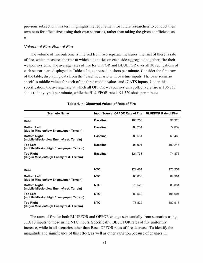
81

previous subsection, this term highlights the requirement for future researchers to conduct their own tests for effect sizes using their own scenarios, rather than taking the given coefficients as-is.

Volume of Fire: Rate of Fire

The volume of fire outcome is inferred from two separate measures; the first of these is rate of fire, which measures the rate at which all entities on each side aggregated together, fire their weapon systems. The average rates of fire for OPFOR and BLUEFOR over all 30 replications of each scenario are displayed in Table 4.14, expressed in shots per minute. Consider the first row of the table, displaying data from the “base” scenario with baseline inputs. The base scenario specifies middle values for each of the three middle values and JCATS inputs. Under this specification, the average rate at which all OPFOR weapon systems collectively fire is 106.753 shots (of any type) per minute, while the BLUEFOR rate is 91.320 shots per minute

Table 4.14: Observed Values of Rate of Fire

Scenario Name Input Source OPFOR Rate of Fire BLUEFOR Rate of Fire

Base Baseline 106.753 91.320

Bottom Left (dug-in Mission/low Enemy/open Terrain)

Baseline 85.284 72.039

Bottom Right (mobile Mission/low Enemy/rest. Terrain)

Baseline 80.561 69.466

Top Left (mobile Mission/high Enemy/open Terrain)

Baseline 91.991 100.244

Top Right (dug-in Mission/high Enemy/rest. Terrain)

Baseline 121.733 74.875

Base NTC 122.461 173.251

Bottom Left (dug-in Mission/low Enemy/open Terrain)

NTC 80.033 84.981

Bottom Right (mobile Mission/low Enemy/rest. Terrain)

NTC 75.526 83.831

Top Left (mobile Mission/high Enemy/open Terrain)

NTC 80.562 198.694

Top Right (dug-in Mission/high Enemy/rest. Terrain)

NTC 75.822 182.918

The rates of fire for both BLUEFOR and OPFOR change substantially from scenarios using

JCATS inputs to those using NTC inputs. Specifically, BLUEFOR rates of fire uniformly increase, while in all scenarios other than Base, OPFOR rates of fire decrease. To identify the magnitude and significance of this effect, as well as other variation because of changes in

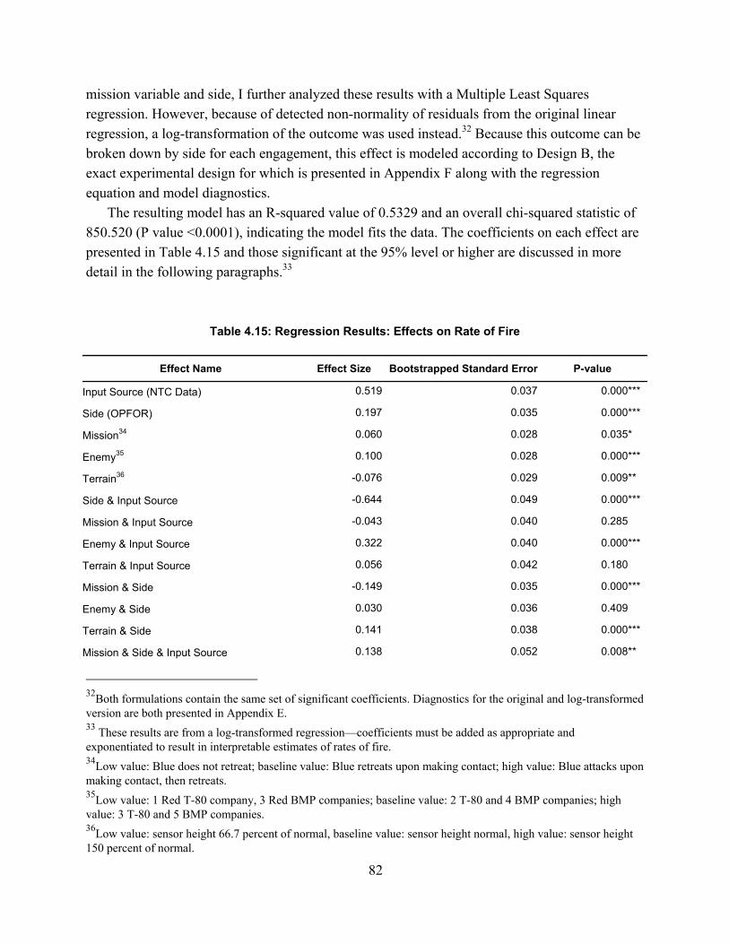
82

mission variable and side, I further analyzed these results with a Multiple Least Squares regression. However, because of detected non-normality of residuals from the original linear regression, a log-transformation of the outcome was used instead.32 Because this outcome can be broken down by side for each engagement, this effect is modeled according to Design B, the exact experimental design for which is presented in Appendix F along with the regression equation and model diagnostics.

The resulting model has an R-squared value of 0.5329 and an overall chi-squared statistic of 850.520 (P value <0.0001), indicating the model fits the data. The coefficients on each effect are presented in Table 4.15 and those significant at the 95% level or higher are discussed in more detail in the following paragraphs.33

Table 4.15: Regression Results: Effects on Rate of Fire

Effect Name Effect Size Bootstrapped Standard Error P-value

Input Source (NTC Data) 0.519 0.037 0.000***

Side (OPFOR) 0.197 0.035 0.000***

Mission34 0.060 0.028 0.035***

Enemy35 0.100 0.028 0.000***

Terrain36 -0.076 0.029 0.009***

Side & Input Source -0.644 0.049 0.000***

Mission & Input Source -0.043 0.040 0.285***

Enemy & Input Source 0.322 0.040 0.000***

Terrain & Input Source 0.056 0.042 0.180***

Mission & Side -0.149 0.035 0.000***

Enemy & Side 0.030 0.036 0.409***

Terrain & Side 0.141 0.038 0.000***

Mission & Side & Input Source 0.138 0.052 0.008***

32Both formulations contain the same set of significant coefficients. Diagnostics for the original and log-transformed version are both presented in Appendix E. 33 These results are from a log-transformed regression—coefficients must be added as appropriate and exponentiated to result in interpretable estimates of rates of fire. 34Low value: Blue does not retreat; baseline value: Blue retreats upon making contact; high value: Blue attacks upon making contact, then retreats. 35Low value: 1 Red T-80 company, 3 Red BMP companies; baseline value: 2 T-80 and 4 BMP companies; high value: 3 T-80 and 5 BMP companies. 36Low value: sensor height 66.7 percent of normal, baseline value: sensor height normal, high value: sensor height 150 percent of normal.

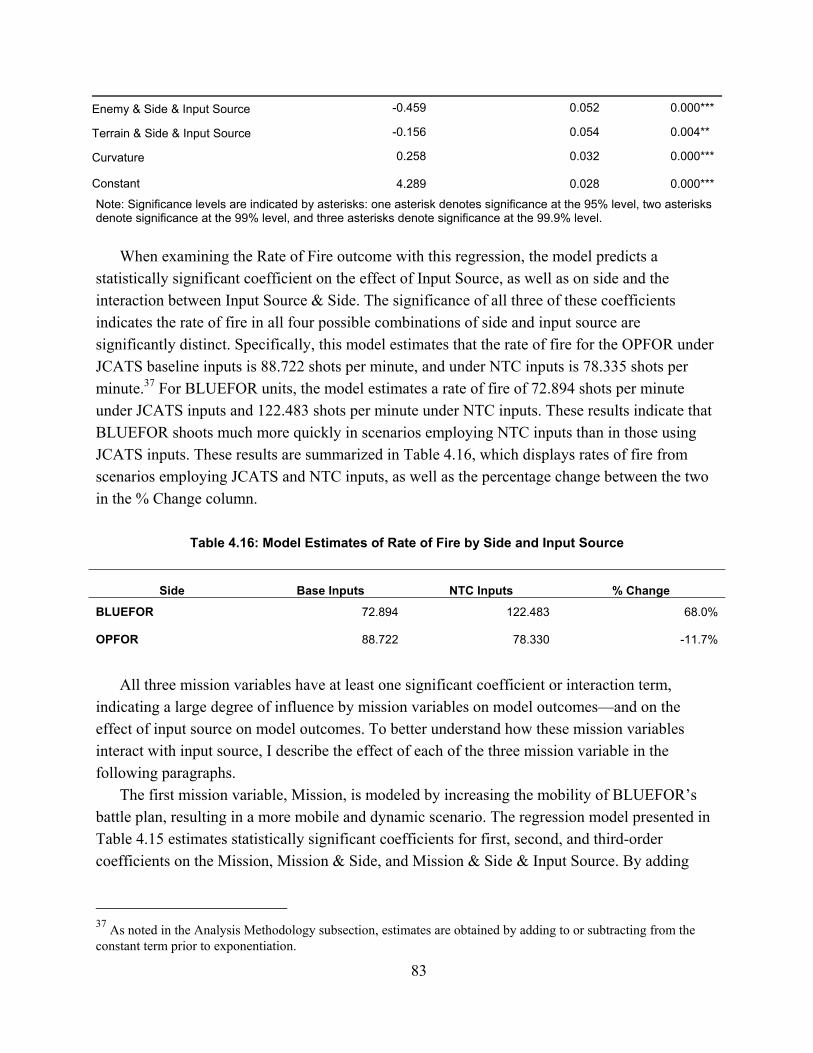
83

Enemy & Side & Input Source -0.459 0.052 0.000***

Terrain & Side & Input Source -0.156 0.054 0.004***

Curvature 0.258 0.032 0.000***

Constant 4.289 0.028 0.000***

Note: Significance levels are indicated by asterisks: one asterisk denotes significance at the 95% level, two asterisks denote significance at the 99% level, and three asterisks denote significance at the 99.9% level.

When examining the Rate of Fire outcome with this regression, the model predicts a

statistically significant coefficient on the effect of Input Source, as well as on side and the interaction between Input Source & Side. The significance of all three of these coefficients indicates the rate of fire in all four possible combinations of side and input source are significantly distinct. Specifically, this model estimates that the rate of fire for the OPFOR under JCATS baseline inputs is 88.722 shots per minute, and under NTC inputs is 78.335 shots per minute.37 For BLUEFOR units, the model estimates a rate of fire of 72.894 shots per minute under JCATS inputs and 122.483 shots per minute under NTC inputs. These results indicate that BLUEFOR shoots much more quickly in scenarios employing NTC inputs than in those using JCATS inputs. These results are summarized in Table 4.16, which displays rates of fire from scenarios employing JCATS and NTC inputs, as well as the percentage change between the two in the % Change column.

Table 4.16: Model Estimates of Rate of Fire by Side and Input Source

Side Base Inputs NTC Inputs % Change

BLUEFOR 72.894 122.483 68.0%

OPFOR 88.722 78.330 -11.7%

All three mission variables have at least one significant coefficient or interaction term,

indicating a large degree of influence by mission variables on model outcomes—and on the effect of input source on model outcomes. To better understand how these mission variables interact with input source, I describe the effect of each of the three mission variable in the following paragraphs.

The first mission variable, Mission, is modeled by increasing the mobility of BLUEFOR’s battle plan, resulting in a more mobile and dynamic scenario. The regression model presented in Table 4.15 estimates statistically significant coefficients for first, second, and third-order coefficients on the Mission, Mission & Side, and Mission & Side & Input Source. By adding

37 As noted in the Analysis Methodology subsection, estimates are obtained by adding to or subtracting from the constant term prior to exponentiation.

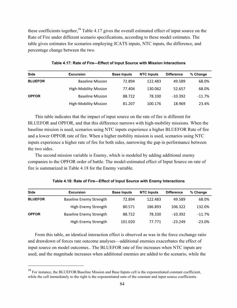
84

these coefficients together,38 Table 4.17 gives the overall estimated effect of input source on the Rate of Fire under different scenario specifications, according to these model estimates. The table gives estimates for scenarios employing JCATS inputs, NTC inputs, the difference, and percentage change between the two.

Table 4.17: Rate of Fire—Effect of Input Source with Mission Interactions

Side Excursion Base Inputs NTC Inputs Difference % Change

BLUEFOR Baseline Mission 72.894 122.483 49.589 68.0%

High‐Mobility Mission 77.404 130.062 52.657 68.0%

OPFOR Baseline Mission 88.722 78.330 ‐10.392 ‐11.7%

High‐Mobility Mission 81.207 100.176 18.969 23.4%

This table indicates that the impact of input source on the rate of fire is different for

BLUEFOR and OPFOR, and that this difference narrows with high-mobility missions. When the baseline mission is used, scenarios using NTC inputs experience a higher BLUEFOR Rate of fire and a lower OPFOR rate of fire. When a higher mobility mission is used, scenarios using NTC inputs experience a higher rate of fire for both sides, narrowing the gap in performance between the two sides.

The second mission variable is Enemy, which is modeled by adding additional enemy companies to the OPFOR order of battle. The model-estimated effect of Input Source on rate of fire is summarized in Table 4.18 for the Enemy variable.

Table 4.18: Rate of Fire—Effect of Input Source with Enemy Interactions

Side Excursion Base Inputs NTC Inputs Difference % Change

BLUEFOR Baseline Enemy Strength 72.894 122.483 49.589 68.0%

High Enemy Strength 80.571 186.893 106.322 132.0%

OPFOR Baseline Enemy Strength 88.722 78.330 ‐10.392 ‐11.7%

High Enemy Strength 101.020 77.771 ‐23.249 ‐23.0%

From this table, an identical interaction effect is observed as was in the force exchange ratio

and drawdown of forces rate outcome analyses—additional enemies exacerbates the effect of input source on model outcomes.. The BLUEFOR rate of fire increases when NTC inputs are used, and the magnitude increases when additional enemies are added to the scenario, while the

38 For instance, the BLUEFOR/Baseline Mission and Base Inputs cell is the exponentiated constant coefficient, while the cell immediately to the right is the exponentiated sum of the constant and input source coefficients.

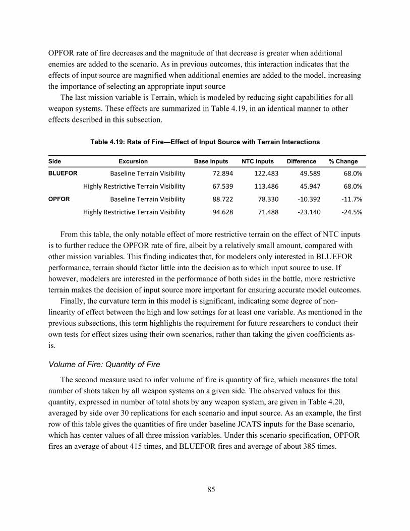
85

OPFOR rate of fire decreases and the magnitude of that decrease is greater when additional enemies are added to the scenario. As in previous outcomes, this interaction indicates that the effects of input source are magnified when additional enemies are added to the model, increasing the importance of selecting an appropriate input source

The last mission variable is Terrain, which is modeled by reducing sight capabilities for all weapon systems. These effects are summarized in Table 4.19, in an identical manner to other effects described in this subsection.

Table 4.19: Rate of Fire—Effect of Input Source with Terrain Interactions

Side Excursion Base Inputs NTC Inputs Difference % Change

BLUEFOR Baseline Terrain Visibility 72.894 122.483 49.589 68.0%

Highly Restrictive Terrain Visibility 67.539 113.486 45.947 68.0%

OPFOR Baseline Terrain Visibility 88.722 78.330 ‐10.392 ‐11.7%

Highly Restrictive Terrain Visibility 94.628 71.488 ‐23.140 ‐24.5%

From this table, the only notable effect of more restrictive terrain on the effect of NTC inputs

is to further reduce the OPFOR rate of fire, albeit by a relatively small amount, compared with other mission variables. This finding indicates that, for modelers only interested in BLUEFOR performance, terrain should factor little into the decision as to which input source to use. If however, modelers are interested in the performance of both sides in the battle, more restrictive terrain makes the decision of input source more important for ensuring accurate model outcomes.

Finally, the curvature term in this model is significant, indicating some degree of non-linearity of effect between the high and low settings for at least one variable. As mentioned in the previous subsections, this term highlights the requirement for future researchers to conduct their own tests for effect sizes using their own scenarios, rather than taking the given coefficients as-is.

Volume of Fire: Quantity of Fire

The second measure used to infer volume of fire is quantity of fire, which measures the total number of shots taken by all weapon systems on a given side. The observed values for this quantity, expressed in number of total shots by any weapon system, are given in Table 4.20, averaged by side over 30 replications for each scenario and input source. As an example, the first row of this table gives the quantities of fire under baseline JCATS inputs for the Base scenario, which has center values of all three mission variables. Under this scenario specification, OPFOR fires an average of about 415 times, and BLUEFOR fires and average of about 385 times.

86

Table 4.20: Observed Values of Quantity of Fire

Scenario Name Input Source OPFOR Quantity of Fire BLUEFOR Quantity of Fire

Base Baseline 415.067 385.567

Bottom Left (dug-in Mission/low Enemy/open Terrain)

Baseline 367.067 479.567

Bottom Right (mobile Mission/low Enemy/rest. Terrain)

Baseline 309.100 326.833

Top Left (mobile Mission/high Enemy/open Terrain)

Baseline 399.600 346.867

Top Right (dug-in Mission/high Enemy/rest. Terrain)

Baseline 559.967 819.333

Base NTC 875.500 483.533

Bottom Left (dug-in Mission/low Enemy/open Terrain)

NTC 654.933 412.467

Bottom Right (mobile Mission/low Enemy/rest. Terrain)

NTC 389.300 322.733

Top Left (mobile Mission/high Enemy/open Terrain)

NTC 1085.033 344.267

Top Right (dug-in Mission/high Enemy/rest. Terrain)

NTC 2596.333 505.700

Upon first look at these results, the OPFOR quantity of fire appears to dramatically increase

when NTC inputs are used in lieu of JCATS inputs. The BLUEFOR quantity of fire changes when input sources are changed, but the difference is not uniform and is not of large magnitude (relative to the changes in OPFOR quantity). To precisely identify the magnitude and significance of this effect, as well as other variation because of changes in mission variable and side, I further analyzed these results with a Multiple Least Squares regression. Because this outcome can be broken down by side for each engagement, this effect is modeled according to Design B, the exact experimental design for which is presented in Appendix F along with the regression equation and model diagnostics.

The resulting model has an R-squared value of 0.677 and an overall chi-squared statistic of 687.520 (P value <0.0001). Again due to non-normality of residuals, a log-transformation of the dependent variable in this regression was conducted, meaning that the coefficients in the following table must be exponentiated to arrive at estimates of shot volume. Those coefficients significant at the 95% level or higher are discussed in more detail in the following paragraphs.

Table 4.21: Regression Results: Effects on Quantity of Fire

Effect Name Effect Size Bootstrapped Standard Error P-value

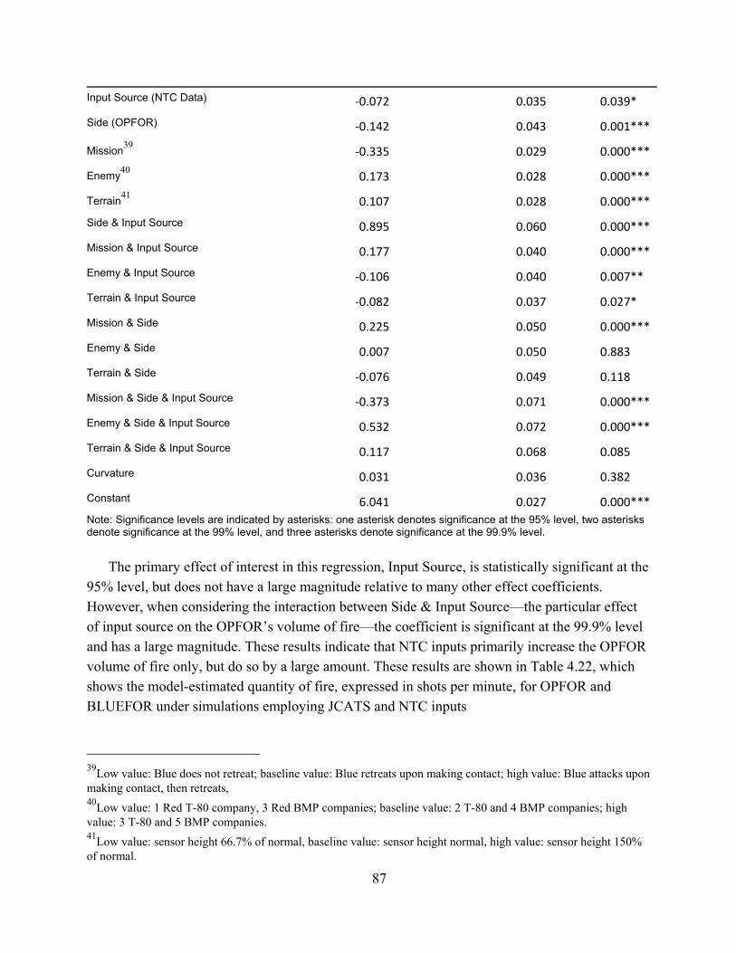
87

Input Source (NTC Data) ‐0.072 0.035 0.039***

Side (OPFOR) ‐0.142 0.043 0.001***

Mission39

‐0.335 0.029 0.000***

Enemy40

0.173 0.028 0.000***

Terrain41

0.107 0.028 0.000***

Side & Input Source 0.895 0.060 0.000***

Mission & Input Source 0.177 0.040 0.000***

Enemy & Input Source ‐0.106 0.040 0.007***

Terrain & Input Source ‐0.082 0.037 0.027***

Mission & Side 0.225 0.050 0.000***

Enemy & Side 0.007 0.050 0.883***

Terrain & Side ‐0.076 0.049 0.118***

Mission & Side & Input Source ‐0.373 0.071 0.000***

Enemy & Side & Input Source 0.532 0.072 0.000***

Terrain & Side & Input Source 0.117 0.068 0.085***

Curvature 0.031 0.036 0.382***

Constant 6.041 0.027 0.000***

Note: Significance levels are indicated by asterisks: one asterisk denotes significance at the 95% level, two asterisks denote significance at the 99% level, and three asterisks denote significance at the 99.9% level.

The primary effect of interest in this regression, Input Source, is statistically significant at the

95% level, but does not have a large magnitude relative to many other effect coefficients. However, when considering the interaction between Side & Input Source—the particular effect of input source on the OPFOR’s volume of fire—the coefficient is significant at the 99.9% level and has a large magnitude. These results indicate that NTC inputs primarily increase the OPFOR volume of fire only, but do so by a large amount. These results are shown in Table 4.22, which shows the model-estimated quantity of fire, expressed in shots per minute, for OPFOR and BLUEFOR under simulations employing JCATS and NTC inputs

39Low value: Blue does not retreat; baseline value: Blue retreats upon making contact; high value: Blue attacks upon making contact, then retreats, 40Low value: 1 Red T-80 company, 3 Red BMP companies; baseline value: 2 T-80 and 4 BMP companies; high value: 3 T-80 and 5 BMP companies. 41Low value: sensor height 66.7% of normal, baseline value: sensor height normal, high value: sensor height 150% of normal.

88

Table 4.22: Model Estimates of Quantity of Fire by Side and Input Source

Side Base Inputs NTC Inputs % Change

BLUEFOR 420.341 391.102 -7.0%

OPFOR 364.684 830.409 127.7%

The estimates of all three mission variable coefficients and their interaction terms in this

model include at least one statistically significant term, indicating a degree of influence by mission variables on both model outcomes and on the effect of input source on model outcomes. To better understand how these mission variables impact the effect of input source, I examine in detail the effect of each of the three mission variables in the following paragraphs.

The first mission variable effect, that of Mission, indicates that, when BLUEFOR has a higher-mobility mission and when NTC inputs are used, the OPFOR fires its weapons less over the simulation run than in runs with other specifications. The exact effect of Input Source on quantity of shots depends on the scenario specifications, as summarized in Table 4.23.42

Table 4.23: Quantity of Fire—Effect of Input Source with Mission Interactions

Side Excursion Base Inputs NTC Inputs Difference % Change

BLUEFOR Baseline Mission 420.341 391.102 ‐29.239 ‐7.0%

High‐Mobility Mission 300.763 334.160 33.396 11.1%

OPFOR Baseline Mission 364.684 830.409 465.724 127.7%

High‐Mobility Mission 326.894 612.159 285.265 87.3%

The results presented in this table indicate that the impact of the Mission variable on the

effect of NTC inputs is to narrow the gap between BLUEFOR and OPFOR effects. The BLUEFOR effect turns from a small negative effect to a small positive effect, while the magnitude of the OPFOR effect is cut nearly in half. Thus, the effect of NTC inputs on OPFOR and BLUEFOR converges when BLUEFOR is engaged in a high-mobility mission.

The second mission variable, Enemy indicates that, when additional OPFOR combat power is added to their order of battle, OPFOR quantity of fire dramatically increases. This increase in input source effect on the outcome is not matched by a substantial change for the effect on BLUEFOR quantity of fire. The detailed interaction effects of Enemy on the effect of input source are described in Table 4.24 for each scenario specification.

42 Again, the values in this table were transformed back to estimates of shot volume to ease interpretation.

89

Table 4.24: Quantity of Fire—Effect of input Source with Enemy Interactions

Side Excursion Base Inputs NTC Inputs Difference % Change

BLUEFOR Baseline Enemy Strength 420.341 391.102 ‐29.239 ‐7.0%

High Enemy Strength 499.509 417.926 ‐81.584 ‐16.3%

OPFOR Baseline Enemy Strength 364.684 830.409 465.724 127.7%

High Enemy Strength 433.370 1511.115 1077.745 248.7%

This table indicates that, when enemy strength is increased, the effect of NTC inputs on

overall quantity of fire is exacerbated. This is an unsurprising result—if NTC inputs increase overall OPFOR quantity of fire, then increasing the number of OPFOR in the scenario should also increase the effect by at least a proportional amount, which is seen in these results.

The last mission variable is Terrain, which describes how the impact of input source changes when the sight lines of all weapon systems are reduced, simulating more restrictive terrain. These effects are summarized in Table 4.25, in an identical manner to other effects described in this subsection.

Table 4.25: Quantity of Fire—Effect of Input Source with Terrain Interactions

Side Excursion Base Inputs NTC Inputs Difference % Change

BLUEFOR Baseline Terrain Visibility 420.341 391.102 ‐29.239 ‐7.0%

Highly Restrictive Terrain Visibility 467.815 400.847 ‐66.968 ‐14.3%

OPFOR Baseline Terrain Visibility 364.684 830.409 465.724 127.7%

Highly Restrictive Terrain Visibility 405.872 851.099 445.227 109.7%

The differences in results presented in this table are small in terms of percentage change, particularly when compared to other effect sizes. Still, these results indicate that the relative effect of NTC inputs on both the OPFOR and BLUEFOR are reduced by a small amount in restrictive terrain. This reduction makes intuitive sense, as restrictive terrain will reduce the number of possible shots by reducing the detection capabilities of any given weapon system—which is seen in these results. The final coefficient of note, on the curvature term, indicates that these estimates are largely linear between the high and low settings of each mission variable. This finding signals that, within the bounds of the scenario tested in this dissertation, estimates of quantity of fire can be accurately predicted with the fitted model. However, as with other estimates presented in this dissertation, extrapolation of these results to other models or to settings of mission variables not

90

tested here will result in unknown bias—researchers should subject models to their own tests to determine the specific effect of input data on their scenario.

Discussion

One of the primary goals of this research was to determine whether NTC inputs instead of the JCATS baseline inputs had an effect on model outcomes. For all four of the outcome measures examined, there were large and statistically significant differences between runs that employed JCATS baseline inputs and runs that used NTC inputs. As an example, for the force exchange ratio outcome, the effect was observed across mission conditions but it was differentially affected as the enemy task organization changed: the exchange ratio is lower (less favorable to BLUEFOR) when additional enemy companies were included in the scenario and when NTC inputs were used in lieu of baseline inputs.

In addition to this difference, I found that the input source affected the outcomes differentially as the mission conditions changed. For instance, the results from the volume of fire outcomes showed that in general BLUEFOR fired more rapidly and OPFOR fired more total shots. However, many mission-variable-by-input-source interaction effects were statistically significant, indicating that the effect of input source varies as the conditions varied. Of these interaction effects however, only one was consistent across all outcomes; that of Enemy, which was modeled by adding or subtracting two companies from the OPFOR order of battle.

In the remainder of this chapter, I discuss in greater detail these two key takeaways; that the baseline inputs are more favorable to BLUEFOR, and that the effects of NTC inputs are more pronounced with additional enemies.

Baseline Inputs Are Favorable to BLUEFOR

Overall, BLUEFOR was successful in the scenario employed for this dissertation in terms of force exchange ratios and drawdown of forces under both NTC and JCATS inputs; however, that is a merely a reflection of the scenario used and not of particular interest. Of interest is if and how using inputs derived from the NTC would change scenario outcomes. This research finds that, across all outcome measures, there was a consistent pattern in which using the NTC inputs would decrease the differences between Red and Blue relative to when the JCATS inputs were used. In other words, the JCATS input make it appear that Blue significantly overmatches Red; however, when input derived from realistic training are applied, the degree of Blue overmatch diminishes greatly.

Take the force exchange ratio, which can most closely be tied to a unit’s overall performance in the simulation. With this outcome, the difference in ratio between scenarios using NTC inputs and those using JCATS inputs was -0.09, a substantial decrease. A similar trend is seen when examining the drawdown of forces rates which increase for the BLUEFOR and decrease for the OPFOR in scenarios using NTC inputs. Finally, the two volume of fire measures indicate that the

91

BLUEFOR fires more rapidly, while the OPFOR fires more shots overall when NTC inputs are used—a finding that holds across nearly all mission variables.

Across each of these outcomes, a pattern becomes clear. Scenarios utilizing NTC-based input data result in less BLUEFOR overmatch of OPFOR. This pattern should not suggest that JCATS inputs are useless and should be discarded—indeed, JCATS and NTC inputs produce ordinally identical results. Rather, JCATS inputs represent a more optimistic state of the world than do NTC inputs, a difference that simulation modelers should be cognizant of and account for when creating scenarios, or when making decisions based on scenario outcomes.

Effects of NTC Inputs Are More Pronounced with Additional Enemies

In addition, the effects of NTC inputs on model outcomes become more pronounced when OPFOR systems are added to the scenario. For the force exchange ratio, the rate becomes even more equitable when both NTC inputs and additional enemy systems are used in a scenario (0.737 compared with 0.787 for scenarios with a baseline number of enemies). For the drawdown of forces rate, the effect of NTC inputs on loss rate converges when additional enemies are added to the scenario, from an increase of 1.95 and 12.70 for BLUEFOR and OPFOR, respectively, with baseline numbers of enemy systems to 2.98 and 9.38 for BLUEFOR and OPFOR, respectively. Finally, for volume of fire, additional enemies exacerbate the directions of both rate of fire and quantity of fire for both sides. Taken together, these findings suggest that any differences in outcome resulting from input data will be exacerbated by adding additional OPFOR weapon systems to the scenario.

92

5. Conclusions and Policy Recommendations

In this final chapter, I provide some conclusions and some policy recommendations based on the results from this dissertation. I conclude with some suggestions for further research.

Conclusions

This dissertation included a through literature review of current input sources for simulation models and an exposition on new methodologies for measure derivation. Based on past research, I identified a potential gap in current mounted maneuver simulation modeling: inputs based on realistic direct fire behaviors. I derived measures from NTC training events and tested if inputs derived from these data would yield substantially different model results as compared to the input data that currently is in use. The tests revealed that no matter how the variables of mission, enemy, and terrain were changed, that the input source – NTC versus baseline – made a significant difference in all outcomes estimated. The NTC-based measures derived and tested in this dissertation form the starting point for what could be an extremely robust, specific, and representative input source of combat behaviors that could provide significant insights to future acquisition programs.

I analyzed current input data sources for combat modeling and simulation used in support of acquisition processes, to assess the strengths and weaknesses of each. and found that each of the four current sources of input data—historical combat, operational testing, other simulations, and SME judgment -have weaknesses in data quantity, specificity, and/or realism such that no single data source is sufficient. In particular, historical combat and operational testing suffer from a dearth of available data, other simulations suffer from a lack of realism, and SME judgments lack sufficient specificity to be useful for simulation input data. Based on these findings, there is a gap in current input data sources that could be filled with input data from live instrumented training events at the NTC.

I explored historical attempts to measure combat behavior from instrumented combat at the NTC, drawing lessons from each of the four major streams of research.1 I leveraged these previous studies to define methods for analyzing it to produce useful measures of combat behavior in simulation models: weapon system probability of hit, weapon system rate of fire, unit dispersion, and unit speed. I use the four measures to address identified gaps and test model outcomes that result with these “more realistic” inputs. Across each outcome I find that, while both data sources result in generally expected outcomes, the baseline JCATS inputs systematically favor BLUEFOR compared with NTC-based inputs. Furthermore, I find that any

1 The four streams of research were conducted by the RAND Arroyo Center, CALL, ARI, and NPS.

93

differences between input data sources are exacerbated when additional enemies are added to the OPFOR order of battle. These findings indicate that there is significant value to simulation modelers in considering NTC-based inputs for future simulation models; otherwise, they, and the Army, are likely to underestimate adversary armor capability and overestimate blue capabilities. This mis-estimation could negatively affect investment decisions for future armor systems.

The key takeaway from this research for simulation modelers is that parameters of combat behavior based on NTC data do provide a notable difference in model outcomes and represent a potentially rich source of untapped data. The key takeaway for acquisition decision makers is that parameters indicating weapon system behavior in combat may be obtained from NTC data without having to resort to expensive or time-consuming operational tests. The key takeaway for personnel and decision makers at the NTC is that data from the instrumentation system can be of great use for describing unit behaviors in combat and as a new way for providing feedback to rotational training units.

Caveats

Though this research represents an improvement in simulation modeling capabilities, it has three main drawbacks that policymakers and modelers seeking to use its methods and conclusions need to be aware of. First, the NTC data are not perfect—although every effort was made to ensure robustness and accuracy the measures described herein, errata in the data may affect measure values in unforeseen ways. Several means to modify the NTC-IS software and hardware to correct for these errata are outlined below. Second, the test of input data effect on model outcomes conducted in Chapter 4 of this dissertation has only limited generalizability to other simulation models. Each model has a unique way of treating and processing its input data, meaning the effects of NTC data relative to baseline data may change across models. Third, the scenario tested in this dissertation, while created based on an operationally relevant and outside-vetted scenario, is not representative of all possible mission sets. The existence of interaction effects between mission variables and effect of data source on outcomes suggests that the impact of NTC data use on model outcomes could differ if other scenarios are used. Though the trends discussed in this dissertation are broadly applicable, the specific effect sizes presented in Chapter 4 are only directly applicable to the specific JCATS scenarios tested, not to other scenarios or models.

Before delving into the policy recommendations of this dissertation, I offer a cautionary note about what this dissertation does and does not focus on, as well as where the results from this research should and should not be applied. First and foremost, this research represents a proof of concept for a set of measures that attempt to capture direct fire behavior from instrumented training exercises—measures that can then be used to improve weapon system representation in models and simulations.

However, this dissertation does not create a system of performance or readiness measurement. The measures created herein are unsuitable for either use because of two sets of

94

concerns. First, data from the NTC-IS are not of sufficient accuracy on a unit level to serve as readiness or performance measures. While the algorithms described in this dissertation significantly improve data reliability and accuracy from the NTC-IS in its raw form, the measures derived in this dissertation take advantage of hundreds of observations over years of data collection to reliably estimate direct fire behaviors. A single unit participating in a NTC rotation will, by comparison, have very few observations and may contain one or more erroneous data points, introducing a large amount of uncertainty into the overall results.

Second, the NTC is a training environment—the main objective of both the NTC and the rotational units is to ensure each unit ends the rotation at the highest possible level of readiness. Not only does this objective mean that the unit, during most of its time at the NTC, is improving in performance, but it also means that measuring unit performance or readiness would fundamentally alter the training process at NTC. To learn at NTC, the unit must take risks and be willing to make mistakes in order to learn, and the trainers at the NTC must be able to coach them candidly throughout. If the measures described here were to be used for readiness or performance measurement purposes, this training process would be adulterated: Units may become less willing to make risky decisions, trainers may become less willing to offer critical feedback, and, most important, the relationship between rotational unit and trainer would deteriorate, thus stifling potential learning. It is thus critically important that measures derived from NTC-IS not be tied to readiness reporting or to unit-level performance measurement at any level.

Policy Recommendations

I next present recommendations for policy actions that can be taken by the NTC and/or other analytical organizations within the Army.

Apply Measures Derived from NTC Data to Simulation Model Input Data

The methods outlined in this dissertation form the foundation for what could be a much larger and more comprehensive system of behavioral measurement for simulation model data that could prove useful in the acquisition process. The four measures described and tested herein, as well as the additional measures outlined in Appendix C, represent a starting set of measures that are expedient to implement. Additional measures that use more sophisticated analytical techniques are also possible and represent an excellent next step for researchers interested in advancing this methodology.

The tests conducted in this dissertation indicate that baseline simulation inputs in the JCATS model systematically overstate BLUEFOR capabilities and/or understate OPFOR capabilities compared with NTC inputs. Furthermore, the tests concluded that these differences in performance were exacerbated when additional Red forces participate in the battle. These conclusions strongly suggest that the NTC data represent a more difficult state of the world than

95

that described with JCATS data—a state of the world that includes confusion, imperfect training, and an extremely skilled and cunning enemy. The outcome differences are non-trivial and are robust to minor changes to the scenario.

These measures do not describe an ideal picture of the battlefield, nor do they represent the maximum potential combat power of any given weapon system. Rather, they attempt to describe combat as it is actually fought—fraught with confusion and difficulty. These measures should be treated as such by any modeler attempting to use them. In most cases, it will be beneficial to run two sets of scenarios—one in which the maximal capabilities of each weapon system are used to test the best possible case and another in which realistic capabilities based on NTC-derived inputs are used to test a more difficult case. To be effective, a weapon system should perform well under both circumstances.

To implement use of these measures, modelers could take an approach similar to that used in this dissertation; namely, replacing baseline input data with inputs derived from the NTC. First, modelers would identify data in the simulation model that they would like to modify to reflect more difficult battlefield conditions. Next, they would examine the NTC data to identify situations where conditions closely match the simulation scenario. Third, they use would data generated from relevant NTC training events to create measures of combat behavior that can then replace the baseline input data, ideally after validating any newly created measures. This procedure can be time intensive, but is effective in reflecting conditions at NTC in the simulation model. Additionally, once measures are created and validated, they could be included in future releases of the simulation model with an option for the modeler to select NTC or baseline inputs as appropriate. Such a feature would allow modelers maximum flexibility to efficiently use the most appropriate data source and provide the greatest potential benefit to simulation-based acquisition decisions.

Improve NTC-IS Data Quality

Although the NTC-IS data are sufficient for basic measures such as those discussed in this dissertation, they have a number of weaknesses—highlighted in Chapter 3—that reduce confidence in any measures derived from them. Some solutions to these weaknesses would be extremely expensive and require an overhaul of the entire instrumentation system; however, others would be inexpensive and simple to implement. Most of these improvements would simultaneously improve data reliability and improve the instrumentation system’s utility as a training aid. These improvements are discussed in the following paragraphs.

Improve System ID Numbering Capabilities

The current NTC-IS has a limitation on the amount of unique ID numbers that can be assigned to entities participating in the exercise. This limitation is currently a significant hindrance to both weapon system tracking and to fire-hit pairing, because multiple weapon systems are forced, under the current system, to share a single ID number. Relatedly, a capability

96

to change ID numbers from the command center would aid in tracking and number allocation. Under the current system, ID numbers can only be changed on each individual device, making adjustments to ID allocation once the exercise has begun extremely difficult. This potential improvement would provide the most cost-effective means of improving fire-hit pairing from MILES, thus improving significantly the quality of engagement-based measures, such as probability of hit.

Add Enhanced System Status Identifiers

Another potential upgrade includes adding a set of consistent identifiers in the database that indicate the status of each weapon system. While the current instrumentation system does include an indicator about whether a given weapon system is destroyed or healthy, greater accuracy and fidelity in this category would vastly increase analytic confidence and capability. First, a data field that indicates when entities are boresighting, down for maintenance, or inactive—ideally with separate codes—would greatly help filter out data unrelated to physical contact. Second, a data field that indicates when main battle period starts and concludes in each rotation would help categorize data by battle, further filtering out non-physical-contact data.

Add Capability to Locate Points of Impact

A third NTC-IS improvement is an indication of the precise point of impact for every shot, regardless of if it hit a target or not. Such a hardware solution could be as simple as an accelerometer mounted to the firing weapon system’s barrel indicating its orientation and angle, as well as a laser rangefinder indicating the distance to target. The remainder of the required calculations could be conducted using software and a detailed terrain map. This information would have several benefits. First, it would allow for greatly improved pairing of fires and hits. The current data source does not have any explicit pair between fires and hits—rather, it relies on inference-based and error-prone algorithms to pair fires and hits. A laser engagement system upgrade that included information on the exact impact point of every shot would remove much of the uncertainty in these algorithms.2 Knowledge on the impact point of each shot would also allow for measures detailing firing patterns for weapon systems and units as a whole, including accuracy.

Improve MILES Feedback to Soldiers

A fourth effective NTC-IS upgrade would be a more enhanced feedback mechanism to soldiers participating in the training exercise. Under the current system, an auditory and visual alarm is sounded on the target vehicle if it is hit or killed. However, the shooting weapon system crew can rarely hear the auditory alarm and the visual alarm is easily missed in the harsh

2Also useful would be a richer laser beam that could carry additional data about the shooting weapon system. However, such an upgrade would likely require an overhaul of the entire MILES system and is thus not recommended here.

97

brightness of the desert or if the system is obscured from view. This missed alarm often results in “overkill,” in which shooting weapon systems will continue to engage a target after it has already been killed, simply because the crew does not realize they have already scored a hit. Solutions to this range from pyrotechnic markers on hit systems simulating the smoke that billows from destroyed systems in real life to software solutions that display to a shooting vehicle’s crew that they killed their target. To enhance realism is to improve the representativeness of the data to actual combat; thus, any improvement in a crew’s feedback will not only improve the quality of the training simulation at NTC but will also improve the accuracy and reliability of NTC-based measures described and tested in this dissertation.

Improve Storage and Computational Power of the NTC-IS Database

The final upgrade suggested by this dissertation is increased storage and computational capacity for the database backend of the instrumentation system. The current system can become overworked in periods of intense combat, as thousands of simultaneous transmissions and events pour into a single central server. A more powerful server would both reduce the amount of dropped events from this server overload and enable the implementation of a more complex (and accurate) fire-hit pairing algorithm. Such an improvement would aid the training mission at NTC by improving battle tracking by Operations Group personnel while simultaneously markedly improving engagement data used to create measures such as those derived and tested in this dissertation.

Suggestions for Additional Research

This dissertation represents a proof of concept for an analytic technique, and it seems that there is great value to be gained by future researchers extending this methodology. Three fruitful directions of research are suggested and discussed in the following paragraphs.

Apply Advanced Analytic Techniques to Data and Measures

The techniques used in this dissertation for data processing and measures derivation are simple by design—given that this research is a proof of concept, the primary goal was to produce valid measures that had any explanatory power. However, research applying the current state of the art in classification and regression machine learning algorithms could result in significant gains in measure reliability, accuracy, and fidelity.3 Several particularly fruitful areas for future researchers to apply these advanced algorithms include the contact creation algorithm, the fire-hit-pairing algorithm, and the regression models used to compute each measure. The contact

3Because the code used for this dissertation was developed using the Python programming language, and because there are a number of extremely feature-rich and widely used packages for applying machine learning algorithms to datasets in Python, the Scikit-Learn package documentation is cited for algorithm references. Researchers are highly encouraged to leverage the extremely powerful open-source tools in this package.

98

creation algorithm is, as currently designed, a custom-built agglomerative clustering algorithm. Clustering is a well-understood and well-researched area of application for machine learning algorithms; applying an advanced clustering algorithm could improve overall performance.4 Similarly, fire-hit-pairing can be conceptualized as a classification problem—each shot event or hit event should have exactly one dyadic counterpart, which can be identified based on a number of event attributes. Currently, this pairing is accomplished with a two-stage algorithm consisting of complex set of filters and an agglomerative clustering algorithm. Applying an advanced classification algorithm could improve matching performance.5 Finally, measure values were calculated in this dissertation using a multiple least squares linear regression—a computationally simple and easily interpretable statistical model. A more sophisticated regression model, such as a random forest6 or a neural network,7 could be applied to measure derivation, with potentially substantial improvements in performance.

Apply Methods to Other Combat Training Centers

This dissertation focuses exclusively on armored combat at the NTC—which is an interesting and well-instrumented but small subset of the missions Army units may undertake. Other missions and unit types train both at NTC and at the other maneuver Combat Training Centers (CTCs), the Joint Readiness Training Center (JRTC) and the Joint Multinational Readiness Center (JMRC). These other CTCs have instrumentation systems as robust as the one at NTC and could similarly provide great benefit for simulation modelers seeking behavioral representations of other unit types. While these centers, their data, and their operational context are unique and require special study prior to any researcher attempting to create measures, this method could be applied with equal validity to these other centers.

Explore Other Uses for Data and Measures

Although this dissertation discusses NTC-based measures of combat behavior purely from a perspective of M&S data, such measures could also be applied with little modification to training processes at the NTC. These measures could be calculated for units while training and used as instructional aides to Operations Group personnel describing to a rotational unit exactly what occurred during each battle period. They could also be analyzed for trends among units, allowing

4For a discussion of open-source clustering algorithms available for implementation in Python and Scikit-Learn, please see http://scikit-learn.org/stable/modules/clustering.html 5For a discussion of open-source classification algorithms available for implementation in Python and Scikit-Learn, please see http://scikit-learn.org/stable/auto_examples/classification/plot_classifier_comparison.html 6For a discussion of open-source Random Forests and other related ensemble machine learning regression algorithms available for implementation in Python and Scikit-Learn, please see http://scikit-learn.org/stable/modules/ensemble.html 7For a discussion of open-source neural network algorithms available for implementation in Python and Scikit-Learn, please see http://scikit-learn.org/stable/modules/neural_networks_supervised.html

99

Operations Group personnel to demonstrate to a unit how they differed from other units in similar situations at NTC.

Extending this other application, the measures created and tested in this dissertation could also be applied toward tactics development. Once trends have been established and tracked at NTC, professional tactics experts at the respective Centers of Excellence throughout the Army could leverage behavior indicated by these measures to create new recommendations for best practices or tactical guidance for operational units.

100

Appendix A: Pairing Fires and Hits in NTC-IS

As discussed in Chapter 3, NTC-IS in its current form does not inherently pair fire and hit events generated by MILES-equipped weapon systems. Rather, a separate shot and hit event is generated by the shooter and the target entity, respectively. At best, the hit event may contain the ID number of the shooter, but even then there is no indication of exactly which shot event caused the hit. As information on fire-hit pairs is considerably more valuable for training purposes than unpaired fire and hit information, efforts have been made throughout the years to algorithmically pair shot and hit events once both are recorded in the database. However, as the algorithm used changes frequently, any analysis that covers a years-long timespan, such as this dissertation, must use a custom pairing algorithm to ensure consistency.

There are two basic mechanisms by which fires and hits can generally be paired, filter-based and likelihood-based. The filter-based methods utilizes a number of binary filters to pare down the potential shot events any hit may be paired with, or any hit events a shot may be paired with, until only one remains. These filters concern the relative attributes of the two events. For instance, in order to pair with a hit event, a shot event’s time must be no more than two seconds before the hit. This is the primary method generally used by NTC-IS administrators.

A second, more computationally intense method calculates a dyadic likelihood for each hit event to be paired with each shot event—the pairs with the highest likelihood are selected. To reduce the amount of computing power required, the set of candidate pairs for any given event can be filtered by some criteria, such as a requirement that the two events must occur within five minutes of one another. This dissertation proposes a version of this method be used to supplement a filter-based approach in a two-step pairing algorithm.

Any fire-hit pairing algorithm must inherently trade off accuracy and completeness. An algorithm with extremely strict match requirements will yield very few matches, but will have an extremely high confidence in each being a valid pair. On the other hand, an algorithm with looser requirements will yield many matches, but at a lower confidence of each being a true match. Because there is no comparison data set of known matches in the NTC-IS database, it is difficult to evaluate an algorithm’s performance relative to these two extremes. Still, in the development of algorithms for this dissertation, every attempt was made to evaluate algorithmic performance, even if such an evaluation is only qualitative in nature. These validation efforts are discussed in detail in Appendix D.

The overall design of the fire-hit pairing used in this dissertation is depicted in Figure A.1. To summarize, it ingests raw NTC-IS data, including a stream of shot events and hit events, as

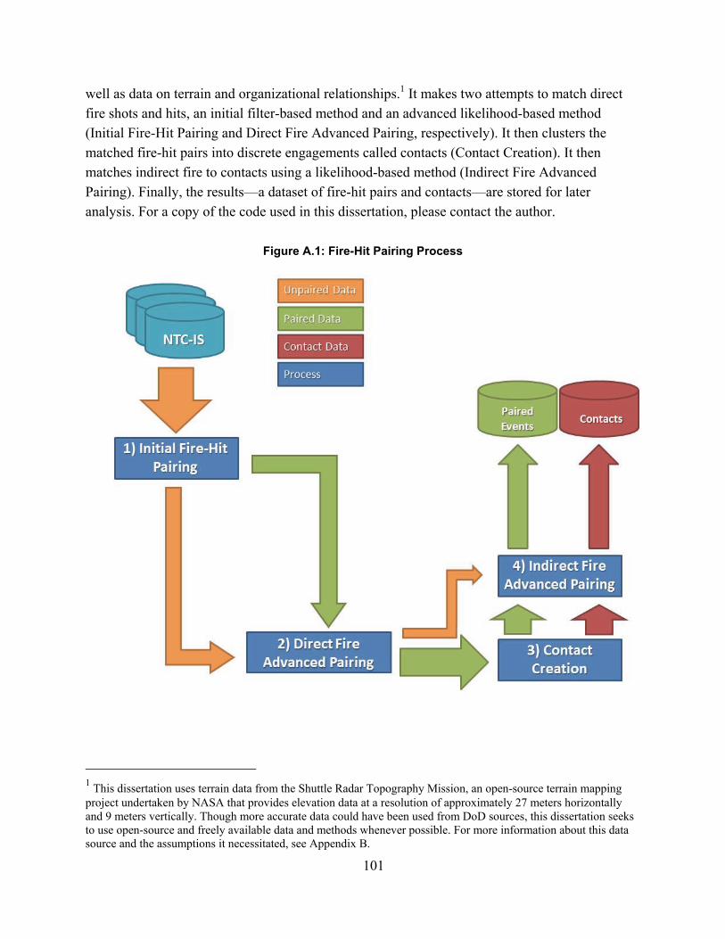
101

well as data on terrain and organizational relationships.1 It makes two attempts to match direct fire shots and hits, an initial filter-based method and an advanced likelihood-based method (Initial Fire-Hit Pairing and Direct Fire Advanced Pairing, respectively). It then clusters the matched fire-hit pairs into discrete engagements called contacts (Contact Creation). It then matches indirect fire to contacts using a likelihood-based method (Indirect Fire Advanced Pairing). Finally, the results—a dataset of fire-hit pairs and contacts—are stored for later analysis. For a copy of the code used in this dissertation, please contact the author.

Figure A.1: Fire-Hit Pairing Process

1 This dissertation uses terrain data from the Shuttle Radar Topography Mission, an open-source terrain mapping project undertaken by NASA that provides elevation data at a resolution of approximately 27 meters horizontally and 9 meters vertically. Though more accurate data could have been used from DoD sources, this dissertation seeks to use open-source and freely available data and methods whenever possible. For more information about this data source and the assumptions it necessitated, see Appendix B.

102

Initial Fire-Hit Pairing

The first step in the pairing process is an algorithm nicknamed “Initial Fire-Hit Pairing”, and is the most similar to the NTC’s current approach to matching fires and hits. This process uses a series of filters to associate events together. The algorithm essentially assumes that events occurring nearly simultaneously at feasible distances, with entities that can see each other, and with appropriate weapon systems are valid matches, especially if the shooter code is available and matches the shooting entity. Following is a description of each of the filters used, as well as a block diagram of the overall algorithm.

Algorithm Description

The algorithm executes one rotation at a time, as it is impossible for shots and hits to be paired between rotations. Once data have been ingested, the algorithm begins by looping over all observed hit events in a rotation. Once these hit events have been validated as suitable for matching in the first filter, the algorithm loops over all shot events, comparing each against filters 2 through 7 to identify candidate matches. Any shot event that passes all six filters is added to a list of candidate pairs for the hit event in question. Once all shot events have been examined, this list of candidate pairs is reduced and, if a single event or events from a single company remain in the candidate list, a pairing is made and added to the database of paired events.

Filter 1: hit event suitability

This filter eliminates hit events that should not be paired whatsoever as they likely represent erroneous data. These erroneous data include weapon systems that are flagged in the system as down for maintenance (as indicated by an organizational name). Second, they also include hits generated as a result of controller guns, as these are irrelevant for the purposes of analysis. Third, they include events that not have any location data, as it is impossible to ascertain line of sight between shooter and target without both valid location data for both events. Finally, they include all mines and Javelin events, which un pair-able as both munitions will generate hit events without a corresponding shot event—these hits are added to the database of paired events as-is. Each of these data types are excluded from consideration for pairing.

Filter 2: shot event suitability

As occurs with hit events, each shot event is checked to ensure it is possible to pair at all. First, if the If the shot event was generated by a controller gun, it is eliminated as these events are irrelevant for the purposes of analysis. Additionally, if a shot matches any of four different indicators of data errors, it is eliminated from consideration: if the shot was fired by a dismounted infantry and is reported as a munition type of “miss,” if the shot has a munition type of “none,” if its organizational name indicates the system is down for maintenance, or if the number of shots reported in the event is zero.

103

Filter 3 munition type match

In this filter, the munition type reported in the shot event is compared against that reported in the hit event. If the two munition types do not match, the shot event is eliminated from consideration. This filter is skipped if the hit event contains an “unknown” munition, which is due to a system error, but can still represent a valid event. If the shot event contains an unknown munition, several potential munition types are inferred based on the weapon system and checked against the munition type reported in the hit event.2

Filter 4: shooter ID

Most MILES lasers will have encoded in them a shooter identification number. This number is reported in both hit events and in shot events. However, due to MILES system errors or mis-assigned ID numbers, that number is sometimes missing or is too generic to allow for system-level matching. If both the shot and hit event contain ID numbers that are valid, an exact match is required to continue through the pairing process. If, however, one or both of the ID numbers reported by the hit and shot events are missing or generic, the potential pair is allowed to continue through the pairing process, though the time filter is tightened to control for the uncertainty introduced into the potential pair by the lack of ID match.

Filter 5: time

Each pair of events is examined for nearness in time. Generally, shots should occur before hits, though due to delays in event propagation or MILES transmission from either system, the shot event could be recorded in the NTC-IS database up to a few seconds after the hit. To account for this potential effect, shot events that occur in a relatively large time window of 30 seconds prior to 10 seconds after the hit event continue through the pairing process, so long as there is an exact ID match in both events. If one or both events does not have a valid ID number, three possible time windows are used, depending on the pair. If the shot event indicates only a single round was fired, a time window of 1 second prior to 0 seconds after the hit event is used. If the hit event indicates a miss, a time window of 3 seconds prior to 0 seconds after is used, because miss events take somewhat longer to propagate through the NTC-IS database than do hit events.3 Finally, if the shot event indicates more than one round was fired, the window dramatically increases to 9 seconds prior to 0 seconds after, each adjusted forward 0.1 seconds times the number of shots taken.4

2 For instance, an M2 Bradley could shoot a 25mm round, a TOW missile, or a .50 caliber machine gun. 3 Corroborated with NTC-IS administrators. 4 For instance, consider two potential shot events. Shot event A occurs at 12:00:11 AM, does not have an ID number, and indicates 1 round was fired. Shot A could thus potentially be paired to any hit that occurs from 12:00:11 to 12:00:12. Shot event B also occurs at 12:00:11 AM and doesn’t have an ID number, but indicates 15 rounds were fired. Shot B could thus potentially be paired to any hit that occurs from 12:00:12.5 to 12:00:21.5.

104

Filter 6: distance

As stated in Chapter 3, each MILES laser emitter has a maximum range of about 5,000 meters—beyond which it is nearly impossible to score a hit. Additionally, pairs closer than 10 meters are assumed to be impossible due to the extremely narrow MILES laser beam widths at close ranges. AH-64 Apache pairs are assumed to have a maximum possible range of 8,000 meters, as fewer obscurants at altitude increase beam power and make it possible to achieve hits at longer ranges. This distance is taken as a straight-line approximation, without accounting for terrain or the curvature of the Earth.

Filter 7: line of sight

Due to its computational complexity, the line of sight filter is the final check on a potential pair before it is added to the database. This filter uses a line of sight detection algorithm (described in detail in Appendix B) written by the author specifically for the present application. The algorithm uses terrain data at a resolution of approximately 27 meters horizontally and 9 meters vertically to determine if terrain blocks a linear sightline between the shooter and target entities in a potential pair. Due to the resolution of the terrain data as well as the heights of the barrels for each weapon system, entity heights are assumed to be 20.5 meters above the ground.5 This filter is intended to be a gross check on pair feasibility, rather than an absolute determination of whether or not a potential shooter can see a potential target at the time of the shot. Due to the ruggedness and vegetation of NTC terrain, as well as the effect obscurants such as smoke or dust have on the efficacy of MILES lasers, it is nearly impossible to determine precisely if a line of sight does or does not exist at the time of the shot.

Each shot event that passes these six filters (# 2-7) is added to a list of candidate matches for the current hit event. Once all shot events have been examined, the list is evaluated for matches. If the list is empty, the hit event is discarded as un pair-able. If there is a single event in the list, the hit event is paired to that shot event and the match is added to the database. If there are a number of events from the same shooter or the same company, the list trimmed by removing all shot events with an absolute time difference of greater than double the smallest time difference. If only shot events of a single munition type remain in the candidate list after this trimming, the location of the shot is interpolated by averaging the locations of the shot events in the candidate list, and a match is added to the database.6

5 Please see Appendix B for a more in-depth explanation of this entity height assumption 6 Requiring a weapon system match for pairing allows analytic breakdowns by weapon system with greater accuracy.

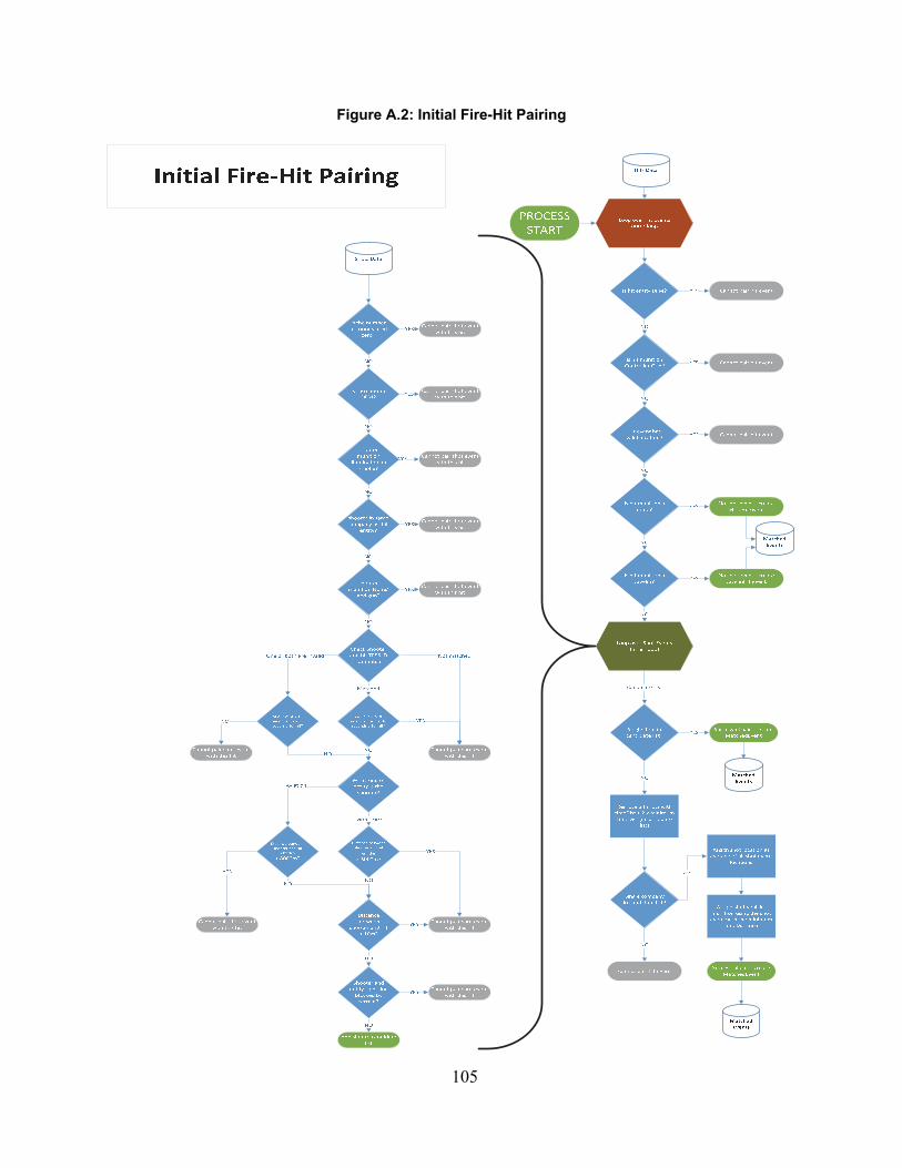
105

Figure A.2: Initial Fire-Hit Pairing

106

Advanced Fire-Hit Pairing

The second step in the fire-hit pairing process is called “Direct Fire Advanced Pairing,” and seeks to pair direct fire shot events that were not matched in Initial Fire-Hit Pairing with their intended target using a likelihood-based pairing algorithm.

I created a framework for this algorithm from knowledge about the NTC and observed patterns of fire-hit pairings, and subsequently extensively tested and iteratively tuned its parameters to ensure the outputs were reasonable. One of the recommendations of this dissertation is to modify the NTC-IS database to include data on the impact point for direct fire munitions. This modification would not only vastly improve pairing accuracy for future rotations, but could provide a set of known data that could then be used to more precisely tune the parameters for this algorithm to retroactively provide higher-fidelity matches for past rotations, thus improving historical analyses. Furthermore, such a set of known data could be used to apply a commercial reinforcement machine learning algorithm to this problem, which reduces the number of assumptions and parameters to tune while increasing pairing accuracy. If modifications to the MILES system are made according to the recommendations of this dissertation, future researchers are highly encouraged to apply such an algorithm to this problem in lieu of the approach described in this subsection.7

Algorithm Description

The algorithm assumes that the entities firing these unpaired events missed their intended target by so wide a margin as to not register on the MILES receiver, but that they were most likely shooting at the same target as other nearby shooters (to include themselves). It models this association by assigning each paired event a likelihood of being associated with a given shot event. This likelihood is calculated using inverse normal transformations of time and physical distance as decrements, as well as static decrements for unit, and weapon system affiliation. Associations are made at the company level and only if the algorithm’s confidence in the association is sufficiently high. Finally, locations are interpolated according to the weighted average of associated fire-hit pair locations, weighted by each event’s likelihood.

A description of the algorithm developed and used in this dissertation is given in the paragraphs below, and a block diagram of its execution is presented in Figure A.3. A validation procedure for this algorithm was also undertaken, the description and results for which can be found in Appendix D.

Step 1: shot event pre-processing

Before beginning the matching process, irrelevant shot events are removed from consideration. First, all events that have already been paired in the initial fire-hit pairing step are removed—these events are later used to evaluate likelihoods of association. Because location 7 See Chapter 5 for a discussion of potential algorithms.

107

plays a large role in determining likelihood of association between a given shot event and a matched pair, the former must have valid location data.8 Finally, shots from controller guns are assumed to be irrelevant and are removed.

Step 2: determine set of candidate matches

Because this process is non-trivially complex, the set of candidate matches that the algorithm calculates likelihood of association for is restricted to those that are feasible to match. The simplest way to filter matched events is by time: matched events that occur more than 15 minutes before or after a given shot event will be assigned a negligible likelihood—small enough to be ignored by this algorithm. Thus, likelihoods of association are only calculated for matched events that occur within 15 minutes of a given shot event.

Step 3: Calculate Time and Distance Standard Deviations

Before assigning likelihoods for each candidate paired event, the standard deviations used in the inverse normal transformations of the time and physical distance between events is calculated. These standard deviations are based on the number of candidate matches—a larger number of candidates indicates a denser collection of shots and hits, and indicates the algorithm should be stricter about assigning likelihoods. These standard deviations are set according to the following two formulae:

.

Max#

1000

,

.

#

1000

,

Where

215

50

320

100

8 The latter must have location data in order to be paired in the first place—see the algorithm description for Initial Fire-Hit Pairing

108

As the search window changes, the standard deviation will be scaled according to the following graphs:

Step 4: evaluate likelihood of association with each candidate paired event

The likelihood of association is calculated based on “nearness” of a given unmatched shot event to a matched pair. This concept is approximated by applying an inverse normal distribution to each paired event’s distance and time difference from the unpaired event. A closer paired event in space and time will be “nearer” and will increase the likelihood of its associated unit also being associated with the unpaired event. Sharing a battalion, brigade, or weapon system also increases a paired event’s likelihood of being associated with the unpaired event.

The likelihood that a shot event is associated with an event pair is calculated for each candidate matched event according to the series of formulae below, and is in the range [0,1].

, , ∗ , ∗ , ∗ ,

Where

,

, 2 ∗ 0,∆ ,

, 2 ∗ 0,∆ ,

,

1.0 0.4

0.50.20.0

, 1.0 0.5

∆ ,

∆ ,

109

Step 5: sum likelihoods over candidate companies

The algorithm then aggregates candidate matched events by the unit associated with the current shot event, thus assuming that a given shot is more likely to be associated with a more active unit. Likelihoods that exceed 0.01 are summed for each associated company (even if the match occurred at the battalion level). This aggregation is expressed in the formula below.

, , , 0.01 0

Where

Step 6: evaluate match confidence

Match confidence for this algorithm is evaluated based on discriminability—how well can

the algorithm say that a shot is associated with one company rather than another?

, 1 ,

,

An association with a company and its events is only accepted if the confidence statistic,

, , exceeds 0.8.

Once a company has been selected for association, a hit location and weapon system for the

shot event is interpolated based on the individual likelihoods of the matched events of the associated company. The interpolated location is the weighted average of locations in the candidate company, with weights as confidence of each event, as a proportion of the company total. This summation is expressed in the formula below:

,

,∗

Where

A block diagram of this process is depicted in Figure A.3 below.

110

Figure A.3: Advanced Fire-Hit Pairing

111

Contact Creation

In the fourth step, “Contact Creation,” paired shots and hits are clustered into discrete battles. Contacts form the base of analysis for much of this dissertation, as they provide a discretized means of examining small unit combat. Contacts represent an extremely small fraction of the total time of any NTC rotation. Much of the time is spent briefing, debriefing, resting, or maneuvering, rather than actively shooting. That time, is ignored by the contact detection algorithm, which instead only focuses on the time weapon systems spend in direct, physical contact with the enemy. For the purposes of direct fire combat behavior and the measures derived in this dissertation, this time spent in contact is all that is required. Future researchers may be interested in capturing some aspects of this pre-combat preparation (on exemplary measure, involving boresighting, is discussed in Appendix C).

A contact describes a discrete physical contact action involving an exchange of fire between BLUEFOR and OPFOR weapons systems. It contains a number of matched fire-hit pair events organized into companies. A contact itself has two pieces of data that are relevant for the purposes of the creation algorithm: duration and area. Contact duration is defined as the difference in time between the earliest and latest fire-hit pair contained within it (which also define the contact start/stop time, respectively). Contact area is defined as a convex hull of all shot and hit events that take place as a part of the contact. Each unit also has a contact area, which is an analogous measure that only counts shot or hit events generated by weapon systems assigned to a given unit in the contact.

An individual weapon system cannot be involved in more than one contact at any given time. A unit can be involved in one or several contacts if its member weapon systems are sufficiently far apart and engaged in separate battles. Also, more than one contact may occur simultaneously, again so long as the participants are far enough apart and engaged in different battles. Finally,

Algorithm Description

The process begins by examining each fire-hit pairing successfully matched to this point. It compares each pair of fires and hits with contacts that have already been created. If either unit in the event is involved in a contact that is within fifteen minutes of the shot, and the relevant entity in the event is located near the other entities involved in the contact, the paired fire-hit is added to the contact. If no match can be made, a new contact is created with that fire and hit. Each contact will thus have at a minimum one shot and one hit, though most will contain a substantial number of events. If a unit currently involved in a contact engages with a new unit, any shots originating from that new unit will be added to the current contact. If the new unit was involved in a separate contact simultaneously, it will be merged with the current contact by moving all of the component fire-hit pairs from the separate contact to the current contact.

112

Step 1: sort matched fire-hit pair events

Events are added to contacts in order of decreasing pair confidence, such that contacts are based on the most certain events. This order is: entity-level initial fire-hit pairs, company-level initial fire-hit pairs, initial fire-hit pair fratricides, advanced fire-hit pairs. Mine hits are eliminated, as they do not have a defined shooter and do not represent an exchange of direct fires.9 Additionally, fratricides matched in the Advanced Fire-Hit Pairing process are not added to contacts.10

Step 2: Evaluate existing contacts for association with each event

Drawing from the sorted event list created in the previous step, each event tests for membership in each existing contact. If no membership or association is found, a new contact, is created using the event.

There are three filters used to determine an event’s association with a contact. The first examines the time of the event relative to the contact’s start and end times. If the event is less than 20 minute before the contact start or 20 minutes after the contact end (or occurred during the contact’s duration), the event is considered as having co-occurred with the contact. If the time difference is larger than 20 minutes, no membership association is possible and the next contact is examined.

The second filter examines entity membership. In order to associate an event with a contact, either the shooting or target unit—up to the battalion level—must already be involved in that contact. Membership in the specific part of the unit engaged in the contact is determined using a convex hull of unit locations and a line of sight check. To be considered for membership in a contact, a weapon system matching a given unit must be inside of, or within 250 (company-level match) or 500 (battalion-level match) meters of the convex hull created by all of a unit’s shot and hit events that occur throughout the contact. Furthermore, it must have a direct line of sight to at least one other member of its matched unit at the time of the shot. Of one of these conditions is false, no membership association is possible and the next contact is examined.

The third filter examines unit membership. Because units may sometimes be involved in more than one contact simultaneously, this filter ensures that the group of weapon systems the recently added event is associated with is actually near the contact. This nearness is determined by comparing the centroid of the unit against the convex hull formed by all shot and hit events in the contact. If the current unit centroid (at the time of the shot) is within 500 meters of the contact convex hull, the unit is considered to be currently participating in the contact and the event is associated with the contact.

9 Future researchers may want to include these events in contacts to investigate the impact shaping effects have on contact progression. 10 Advanced Fire-Hit pairs are intended to signify events that were targeting a given unit. Because no unit purposefully targets friendly forces, fratricides matched in the Advanced Fire-Hit Pairing step have no meaningful interpretation.

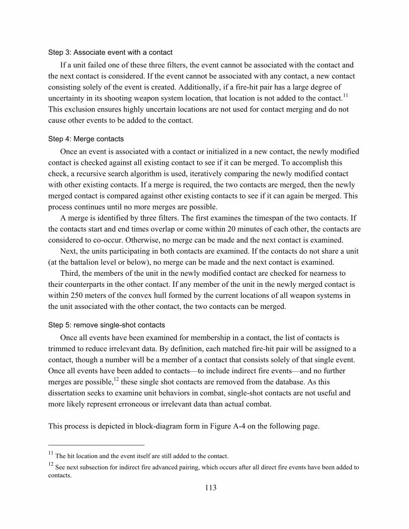
113

Step 3: Associate event with a contact

If a unit failed one of these three filters, the event cannot be associated with the contact and the next contact is considered. If the event cannot be associated with any contact, a new contact consisting solely of the event is created. Additionally, if a fire-hit pair has a large degree of uncertainty in its shooting weapon system location, that location is not added to the contact.11 This exclusion ensures highly uncertain locations are not used for contact merging and do not cause other events to be added to the contact.

Step 4: Merge contacts

Once an event is associated with a contact or initialized in a new contact, the newly modified contact is checked against all existing contact to see if it can be merged. To accomplish this check, a recursive search algorithm is used, iteratively comparing the newly modified contact with other existing contacts. If a merge is required, the two contacts are merged, then the newly merged contact is compared against other existing contacts to see if it can again be merged. This process continues until no more merges are possible.

A merge is identified by three filters. The first examines the timespan of the two contacts. If the contacts start and end times overlap or come within 20 minutes of each other, the contacts are considered to co-occur. Otherwise, no merge can be made and the next contact is examined.

Next, the units participating in both contacts are examined. If the contacts do not share a unit (at the battalion level or below), no merge can be made and the next contact is examined.

Third, the members of the unit in the newly modified contact are checked for nearness to their counterparts in the other contact. If any member of the unit in the newly merged contact is within 250 meters of the convex hull formed by the current locations of all weapon systems in the unit associated with the other contact, the two contacts can be merged.

Step 5: remove single-shot contacts

Once all events have been examined for membership in a contact, the list of contacts is trimmed to reduce irrelevant data. By definition, each matched fire-hit pair will be assigned to a contact, though a number will be a member of a contact that consists solely of that single event. Once all events have been added to contacts—to include indirect fire events—and no further merges are possible,12 these single shot contacts are removed from the database. As this dissertation seeks to examine unit behaviors in combat, single-shot contacts are not useful and more likely represent erroneous or irrelevant data than actual combat. This process is depicted in block-diagram form in Figure A-4 on the following page.

11 The hit location and the event itself are still added to the contact. 12 See next subsection for indirect fire advanced pairing, which occurs after all direct fire events have been added to contacts.

114

Figure A.4: Contact Creation

115

Indirect Fire Advanced Pairing

Though indirect fires are not examined in this dissertation, a method was explored for adding non-lethal indirect fires to contacts. Lethal indirect fires are inherently paired in the NTC-IS database in an entirely separate subsystem from MILES-based direct fire analyzed throughout the rest of this dissertation. However, other indirect fires such as illumination or smoke can still have a sizeable effect on the battlefield, but cannot directly be paired to a hit event. This algorithm seeks to identify the unit that these effects target using a filter-based pairing process after all contacts have been created, but before single-shot contacts have been deleted.

Algorithm Description

Because indirect fire events record an impact location in the database, this algorithm uses the central location of units within contacts to determine “effects” rather than hits. This process loops over each unpaired indirect fire event, examining each contact that is in progress at the time of that fire event, and calculating the weighted average of the locations of each unit in the contact. If the indirect fire event’s hit location is sufficiently near to this convex hull, the fire event is paired to the unit and the pairing is added to the contact.

Step 1: determine if fire event occurred during contact

The algorithm begins by comparing each non-lethal indirect fire event against all existing contacts. If the fire event occurs less than 15 minutes before the start time or 15 minutes after the end time of a contact, the event is considered to occur during that contact. If not, no association is possible and the next contact is examined.

Step 2: determine if fire event impacted a unit

The algorithm then checks the fire event’s point of impact against each unit’s location in the contact. The event is judged as having affected the unit if the point of impact falls inside of or within 300 meters of a convex hull formed by the current locations of the unit’s weapon systems at the time of the shot. If the impact location does not fall within or near the area of any unit, no association is possible and the next contact is examined.

Step 3: resolve conflicts

If the impact location is close to multiple units, the algorithm makes an attempt to resolve the conflict by again determining if the point of impact for an event falls within each unit’s convex hull—this time only impacts strictly inside of the hull are allowed.13 A block diagram of this process is depicted in Figure A.5 on the following page.

13 Other potential conflict resolution solutions do exist, such as associating an event with the closest unit to the point of impact or associating an event with multiple units.

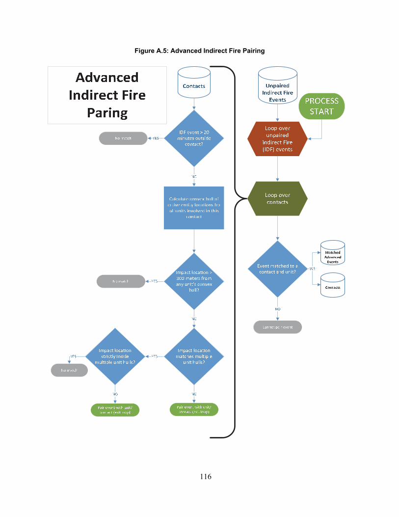
116

Figure A.5: Advanced Indirect Fire Pairing

117

Appendix B: Line of Sight Algorithm Description and Assumptions

The line of sight algorithm I implemented during this research is based on the GRASS GIS14 algorithm for calculating viewsheds of a given point.15 A viewshed is a description (usually a map) of all points that are visible from a starting position.16 It is computationally efficient for the large number of executions required in this analysis—a single processor can calculate over 100 sight lines per second for entities about 2000 meters apart in NTC terrain.17

This algorithm was implemented using the Python programming language, and accounts for not only the terrain between origin and target as well as the curvature of the earth. The terrain is sampled using data from the NASA Shuttle Radar Topography Mission (SRTM), which flew in February, 2000.18 Elevation data from SRTM are available at a 1-arcsecond of latitude and longitude resolution for nearly all landmasses between 60 degrees north and south latitude. At the NTC (about 35 degrees North latitude), this resolution translates to about 30 meters latitude and 25 meters longitude. Any variation in elevation between sample points is not resolved by these data. Additionally, the SRTM data have a vertical height resolution of about nine meters in North America. This data uncertainty presents an acute problem for calculating line of sight in tactical engagements—where vehicles may be mere centimeters above the terrain when firing to maximize protection from enemy fire.

Given these uncertainties, the line of sight criteria is best thought of more in as a blunt instrument used to eliminate clearly impossible shots. Thus, the algorithm is very lenient in establishing line of sight between two entities. This leniency takes the form of entity height above ground level. In addition to the entity’s actual height above the ground, I also add a correction factor to account for sampling height uncertainty and terrain resolution. To account for sampling height uncertainty, I add nine meters to the height of each entity, precluding the possibility that line of sight will be blocked by erroneous terrain.19 To account for possible

14 Geographic Resources Analysis Support System (GRASS) Geographic Information System (GIS) 15 See https://grass.osgeo.org/grass70/manuals/r.viewshed.html. Algorithm is based on Herman Haverkort, Laura Toma, and Yi Zhuang, "Computing Visibility on Terrains in External Memory," ACM Journal on Experimental Algorithmics 13 (2009). 16 While I do not calculate viewsheds due to their computational complexity, such analysis has been used in the past with NTC data and could form an interesting direction for future researchers interested in extending this work. The design of the algorithm, then, provides an extensible base for future researchers to implement viewshed analysis. 17 Based on a test of 500 randomly generated points between 1950 and 2050 meters from a given point within NTC. This algorithm is implemented purely in the Python programming language. It can be considerably accelerated by using a different language, such as C, or by using multiple processors in calculation. 18 Tom G Farr et al., "The Shuttle Radar Topography Mission," Reviews of geophysics 45, no. 2 (2007). 19 This approach is imperfect—for instance, the stated uncertainty of nine meters is given at the 90 percent confidence level, indicating that the value may actually be greater. Additionally, height uncertainty is increased in

118

terrain features unresolved by the data, I make a worst-case assumption based on the M1 Abrams. If one assumes that the M1 can traverse all terrain in a given unresolved area, the side slope limit of 40 degrees becomes the steepest possible terrain in all directions.20 Furthermore, I assume that the hull length of an M1 is 7.92 meters and is width is 3.6 meters,21 along with a resolution of 30 meters in the north-south direction and 25 meters in the east-west direction, and that it is located on flat ground atop a hill.22 These assumptions and the associated distances are displayed graphically below in Figure B.1. The worst case unresolvable height is the minimum height of these two trapezoids: 9.13 meters. I thus increase all entity heights by this amount in all line of sight calculations.

Figure B.1: Line of Sight Data Resolution Correction

Of course, there are many situations where these assumptions would not hold. Vehicles need

not fire from flat ground, and the maximum frontal slope for an M1 Abrams is significantly greater at 60 degrees. Other vehicles have different dimensions and different capabilities for

rugged terrain or sandy and smooth terrain, both of which exist in parts of the NTC. However, without additional elevation data to cross-validate the SRTM data, it is not possible to get a higher-fidelity estimate of error. 20 Though the M1 can traverse terrain up to 60 degrees if approached straight-on, the side-slope limit of 40 degrees is more broadly applicable to most combat systems. 21 "M1A1 Abrams," Military Today, http://www.military-today.com/tanks/m1a1_abrams.htm. 22 Removing the flat-ground requirement would increase the resolution uncertainty correction by about 16.5%

119

traversing terrain. However, I selected these parameters and use them across all line of sight calculations as they apply broadly (the M2/M3 Bradley has similar capabilities and dimensions), and differences between these parameters and those of other vehicles are negligible relative to the magnitude of uncertainties in these calculations.

As a result of these uncertainty corrections, 18.13 meters are added to the actual height of all entities when conducting line of sight calculations. Entities are all assumed to be 2.37 meters tall,23 resulting in a total height of 20.5 meters above ground level.

Though obtaining higher-resolution and more precise elevation data could reduce these worst-case assumptions, using line of sight for precise discrimination of potential shooters is a nearly impossible task due to the unique nature of tactical engagement at NTC as well as the MILES system itself. When defending, entities will often dig into the ground to increase protection form enemy fire, reducing their effective height relative to the ground as depicted by elevation terrain data. With current data sources, it is impossible to determine how far into the ground defenders are dug, if at all. Additionally, shrub vegetation is common at NTC, growing up to several meters tall. Such vegetation commonly blocks MILES lasers, making entities impossible to hit. Due to the ubiquity of such vegetation and its random distribution, it is infeasible to include its location in any line of sight calculation. Thus, the current set of assumptions and line of sight calculations are sufficient for the purposes of pairing fires and hits at NTC.

23 The height of the M1 Abrams turret, "M1A1 Abrams". As with the resolution uncertainty assumption, adjusting this height for each vehicle would result in negligible differences relative to the total uncertainty amount.

120

Appendix C: Additional NTC-IS Measures Not Tested in this Research

In addition to the four measures derived and tested in this dissertation, it is feasible and expedient to extract a number of other measures from the NTC-IS. For a variety of reasons, chiefly that there was no direct input field for many measures into the JCATS simulation model, I explored, but did not fully derive or test these other measures in this dissertation. For the benefit of future researchers, I have included descriptions of each of these other measures in this appendix, categorized by the five aspects of direct fire planning and execution.

Direct Fire Control

Lifting/shifting Fires

This measure seeks to identify situations in which units lift or shift their fires according to changing situations during a contact. It identifies a lifting in fires as a shift in firing on one nearer set of targets to a more distant set of targets as friendly vehicles or troops approach the nearer targets. A shift is more general and is defined as a change in targets from one enemy entity to another during a contact.

Occurrences of lifting fire are identified first by extracting starting and ending times for each contact in the database. The algorithm then retrieves location tracks for each vehicle for a given company during that contact, as well as the locations of all enemy vehicles during the duration of the contact. I then measures the distance between each friendly entity and its nearest enemy for each minute of the contact. The algorithm continues by identifying each engagement during the contact, noting when each vehicle either ceases firing on its target or begins firing on a new target. If the algorithm identifies friendly vehicles firing on an enemy near to an advancing friendly vehicle, the algorithm identifies that engagement as a “near-friendly” engagement. If, while the friendly vehicle continues to advance, its comrade switches targets to an enemy further away, the engagement is identified as a “lift,” and the distance between friendly and enemy is marked. If others in the unit also shift fires, the time taken for the entire unit to complete its lifts is returned as the “time to lift fires.” The average distance between friendly and engaged enemy is also given as the “lifting distance.” These aggregate measures are similarly calculated for shifting fires.

Volume of Fire

This algorithm attempts to ascertain the amount of firepower directed at each enemy entity and unit during contact. Volume of fire is a somewhat nebulous term, but in general it refers to the aggregated rate of fire for all friendly units against the enemy. Thus, the algorithm sums all

121

shots directed at each enemy entity or unit in combat and divides by the time that entity spent in contact. It then aggregates these volumes by taking the total sum of shots directed at a unit’s enemies during all contacts in a rotation and dividing by the total duration of all contacts to arrive at a point estimate of each unit’s volume of fire. To provide an additional level of granularity, this algorithm gives the total volume against companies as well as against individual weapon systems, giving an impression of how directed a given company’s fire was towards specific systems vice a company as a whole.

Time Taken to Return Fire

This measure calculates, for each contact, the time that it took for the unit that was initially fired upon by the initiating unit to return fire against any enemy unit (even if that fire did not hit a target). Note that return fire does not necessarily occur for each contact.

Proportion of Suppressed Systems in Contact

This measure attempts to ascertain to what extent units in contact used suppression against their enemies. NTC-IS represents suppression by disabling a weapon system’s ability to fire for one second after that system has been hit or received a near miss. Thus, the total time that an enemy weapon system was suppressed is the sum of the hits that entity received multiplied by the suppression duration—one second. That time is then divided by the total duration of the contact and is averaged for each side in the contact.

Direct Fire Engagement

Utilization Rate of Assets in Combat

This measure seeks to identify what proportion of a unit’s total combat assets participated in each contact. The algorithm will identify all of the entities within a given company by searching the set of contacts in that rotation and including any entities assigned to a unit that both fired and were fired upon at some point. Due to the nature of the NTC as a training center, nearly every vehicle and crew experiences combat at least once throughout the rotation. Keeping only data from systems that experienced combat will filter out any irrelevant entities, any entities permanently down for maintenance, and other aberrations that may be present in the data. This subset of subordinate entities thus identified, each contact is examined to determine the proportion of each participating unit’s combat assets that were involved. This measure will be aggregated over the rotation by averaging the number over all contacts.1

1 This measure may include contacts of dramatically different lengths and types. Further research into the results of this measure may reveal a need to subdivide this measure into, for example, contacts with a duration of 0-15 minutes, 15-45 minutes, and >45 minutes to account for time required to bring systems to bear against the enemy.

122

Total Shots and Hits Attributed to Each Weapon system

This measure takes a simple total of a company’s shots that it inflicted on all enemies during a contact, as well as a total of hits it suffered from all sources during a contact. It divides these totals by weapon system category involved to ascertain the relative centrality of each weapon system in the contact.

Movement and Maneuver

Mass

This measure evaluates how concentrated any given unit or group of units is at any given time. Mass is measured according to the methodology employed by Geohring and Sulzen; it identifies the proportion of a unit’s assets that are less than one-fourth of the distance from the unit centroid as are the furthest entities from that centroid. As location data are available throughout the rotation, this measure continuously changes. To provide a point estimate, I take the median mass over all times that a particular unit spends in contact with the enemy.

Combined Arms Integration

M7 B-FIST Involvement in Contact with Indirect Fires

The M7 B-FIST contains specialized sighting and communications equipment to enhance indirect fire support to armor and mechanized infantry companies. As such, its use in contacts involving indirect fires will generally enhance the accuracy and effect of those fires. Thus, this measure identifies contacts that included an M7 B-FIST within the area of a unit in contact during the engagement time period and sums them for units and sides.

Number of Contacts Involving Indirect Fires

There are two main ways that indirect fires can affect a battle: shaping enemy actions indirectly, or attempting to directly disable enemy weapon systems. The former can consist of nonlethal means, such as smoke to obscure friendly maneuvers or illumination to highlight enemy positions, or lethal means, such as mines to slow or redirect enemy movement. The latter can consist of precision guided rounds, such as ATACMS, or more suppressive rounds such as Dual Purpose Improved Cluster Munitions (DPICM). This category can also include mortars, though those are generally attached to units at the company level and report directly to the company commander, whereas other indirect fire requires a call for fires directed to units outside of the company. For this reason, mortars are broken out into a third category. Thus, this algorithm counts the number of contacts involving shaping fires, destructive fires, and mortar fires, giving an image of the level of indirect fire support provided to units and the type of that support.

123

Number of Contacts Involving Multiple Maneuver Companies/Helicopter Support

This measure ascertains the complexity of any given contact by determining the number and types of companies that are involved. This algorithm summarizes the different companies that are involved in each combat and counts the number that fire in each. To add a level of granularity, the algorithm also breaks out companies in different types, according to categories assigned by a text parsing algorithm prior to data de-identification. 2 This text parsing algorithm also ensures that each company is represented in the data exactly once. 3 The number of companies of each type are reported in addition to the raw count of companies involved in the contact. These statistics are summarized for each company by counting the number of companies that involved multiple maneuver units in contact.4 Number of contacts involving helicopter support is calculated by summarizing the number of contacts that included fires from combat rotary-wing units.5

Number of Weapon systems Used in Each Contact

Similar to the measure counting number of contacts involving multiple maneuver companies of various types, this measure applies an additional level of granularity by focusing on the individual weapon systems employed in each contact. A company of a given type may include a variety of weapon systems, such as a TOW missile, a 7.62mm machine gun, and a 25mm cannon all within a mechanized infantry company. Each of these weapon systems has different effects on the enemy, and when used in concert, enables the employing force to affect enemy actions to a much greater extent than if they used only one system. In recognition of this synergistic effect, the number and types of weapon systems involved in each contact is calculated and summarized for each company by averaging the number over all contacts throughout the rotation.6

2 Battalion types include: infantry, Field Artillery (FA), armored, cavalry, Brigade Support Battalion (BEB), Brigade Engineer Battalion (BEB), aviation, Combat Sustainment Support Battalion and Other. Company types include: Headquarters and Headquarters Company (HHC), support, command, engineer, mortar, and other (generally combat arms). 3 To ensure consistency, a manual review of the classification of each company was also conducted and any classification errors were corrected prior to data de-identification. 4 Maneuver units are defined as “other” companies that are subordinate to infantry, armored, or cavalry battalions. 5 Combat rotary wing units are defined as “other” companies that are subordinate to aviation brigades. 6 Similar to the utilization rate of units in contact, this measure may vary dramatically depending on different contact lengths and types. Further research into the results of this measure may reveal a need to subdivide this measure into, for example, contacts with a duration of 0-15 minutes, 15-45 minutes, and >45 minutes to account for time required to bring systems to bear against the enemy.

124

Pre-Combat Preparation

Time since Last Boresight/Number of Boresights

This measure uses a special type of contact that was determined in the “contact creation” step of the fire-hit-pairing described above to determine the last time that a unit boresighted their weapons.

Boresighting can occur in two ways at NTC: the first is to use a special piece of equipment that illuminates the point of impact of the lasers directed at it. Units place this device in the field and fire at it from different distances while adjusting their weapons’ sights to ensure the sight is accurate to where the laser beam will impact the target. This method of boresighting generally occurs in the early phases of the rotation, while the unit is still preparing to go into the field. The second way units boresight is by using a friendly vehicle. The unit will park the vehicle in the field, and then fire at it from different distances while adjusting their sights. As the vehicle will flash a light mounted on its roof when it is hit, it provides a similar feedback mechanism as the device used in the early phases of the rotation. This vehicle may be “killed” during the process, but Operations Group personnel are usually on hand to revive the vehicle so it can continue to receive hits.

The algorithm takes advantage of the distinctive character of both methods of boresighting to capture an approximation of the time between units’ boresights. A boresighting contact is separated from a normal contact by the algorithm by identifying all contacts consisting entirely of fratricide that could not be associated with any other contact. This set of fratricide contacts is then filtered into those in which either the shooter or the victim remains stationary while the other gradually moves either closer or further away during the contact. As boresights against the illumination device will not be captured by this algorithm, the simplifying assumption is also made that the “boresighting event” occurred first set of shots generated by each weapon system, unless those events occurred during a contact, in which case the entity did not boresight. The time of the last shot event in last boresighting contact or event is then subtracted from the start time of the current contact to give the time since each entity’s last boresighting. This measure also includes a count of total boresighting events or boresighting contacts for each unit, to give a general image of the level of boresighting each unit engaged in during the rotation.

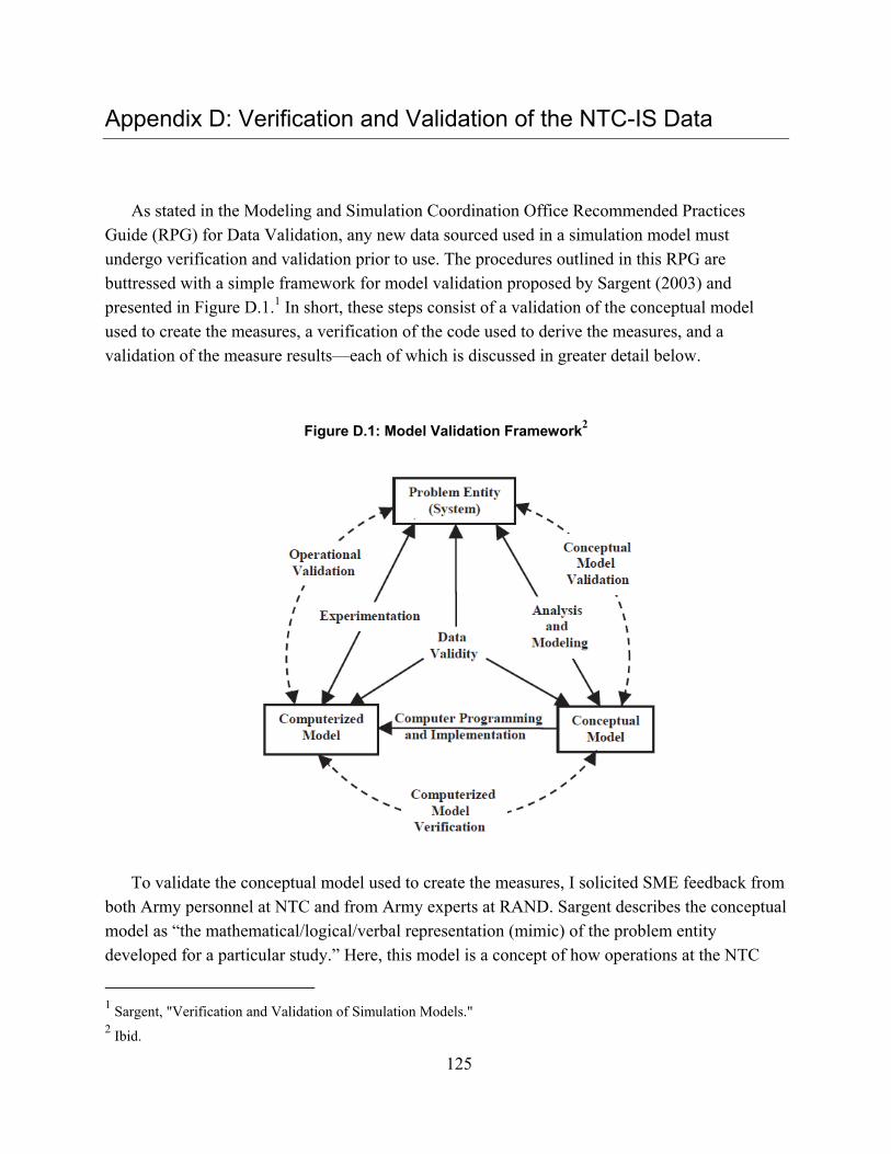
125

Appendix D: Verification and Validation of the NTC-IS Data

As stated in the Modeling and Simulation Coordination Office Recommended Practices Guide (RPG) for Data Validation, any new data sourced used in a simulation model must undergo verification and validation prior to use. The procedures outlined in this RPG are buttressed with a simple framework for model validation proposed by Sargent (2003) and presented in Figure D.1.1 In short, these steps consist of a validation of the conceptual model used to create the measures, a verification of the code used to derive the measures, and a validation of the measure results—each of which is discussed in greater detail below.

Figure D.1: Model Validation Framework2

To validate the conceptual model used to create the measures, I solicited SME feedback from

both Army personnel at NTC and from Army experts at RAND. Sargent describes the conceptual model as “the mathematical/logical/verbal representation (mimic) of the problem entity developed for a particular study.” Here, this model is a concept of how operations at the NTC

1 Sargent, "Verification and Validation of Simulation Models." 2 Ibid.

126

take place, how these operations are currently reflected in instrumentation data, and what inaccuracies or idiosyncrasies may exist in that data. For instance, the conceptual model of the algorithm to pair fires and hits includes an assumption that MILES cannot shoot through terrain, and that events nearer in time are more likely to be associated with each other than events further in time. There are no outputs or results from this portion of the verification and validation process, rather a summary of the process employed is presented.

To verify the computer code used to derive these measures, I examined assumptions both qualitatively and quantitatively. Qualitatively, I worked with my dissertation committee as well as other programmers at RAND and the OIS team at NTC to examine key pieces of analytic code. Quantitatively, I conducted a comprehensive sensitivity analysis of the impact of various assumptions identified in the conceptual model stage of this procedure. In most V&V procedures, sensitivity testing is a form of operational validation by testing how the model’s outcomes respond to changing input parameters. In this dissertation, I instead adjusted assumptions in the data pre-processing stage, such as the maximum engagement distance of various entity types, or the maximum allowable distance in time between a shot and a hit when pairing the two. Ideally, the pre-processing procedure will be robust to changes in any one individual parameter,3 thus indicating a degree of robustness to uncertainty. Additionally, a visual analysis of the impact of each parameter on each model outcome was conducted in order to identify and avoid values in which the model ceases to function normally due to each parameter.

To validate the outcomes produced by the model, I explored the distributions of measures derived from NTC-IS data to ensure that their values are reasonable, and to ensure that various hypothesized effects on measure outcomes are present and statistically significant. As the goal of this system of measurement is was describe the real world, the operational validation component of this study assessed the degree to which measures are valid and reliable, thus appropriately representing the real-world system they purport to represent. Each measure is tested for both face validity—through a qualitative examination of the observed distribution of measure values—as well as convergent/divergent validity through a quantitative examination of correlations with expected effects. Finally, each measure is also tested for reliability through a qualitative examination of potential sources of measurement error (and ways to correct for those sources of error) as well as a quantitative examination of significance levels in an ordinary least squares regression of a number of controls on observed measure values.

Due to data sensitivity, many of the specific values which inform the results of each of these V&V procedures are presented in the restricted-release Appendix E of this dissertation. However, included in the remainder of this Appendix are significance levels, detailed descriptions of the methodology for each component of the process, as well as high-level, qualitative descriptions of results.

3 so long as that parameter is not set to an extreme quantity, such as a maximum engagement distance of zero

127

Conceptual Model Validation

The conceptual model validation utilized a qualitative investigative procedure into assumptions made throughout the measurement process. Specifically, this procedure included explorations of the parameters used in the initial fire-hit pairing process, the advanced fire-hit pairing process, and the contact creation process. It also included assumptions as to the exact form of each of the measures derived from these data.

For the fire-hit pairing stages, the assumptions included the parameters used in the process to determine whether or not a particular hit could be paired to a particular shot. The parameters used would be employed to filter the list of potential shot events down to (ideally) a single shot event that could then be paired with the hit event. To validate these parameters, I discussed the algorithm with NTC personnel familiar with the NTC-IS,4 as well as researchers at RAND knowledgeable of Army operations.

For the contact creation stage, the assumptions included the logic for adding matched events to contacts as well as the thresholds for time and distance for a new event to be included into an existing contact. These assumptions were discussed with NTC personnel familiar with the NTC-IS and RAND researchers knowledgeable of Army operations.

For each of the measures, conceptual model validation was obtained chiefly through a literature review of relevant doctrine and prior measurement studies. Every attempt was made to find a doctrinal definition of each measure and align the derivation of the measure to that doctrinal definition. Additionally, the final formulation of each measure was discussed with RAND researchers familiar with Army operations.

Computerized Model Verification

The RPG for Data Validation recommends that any computational methods used to process or transform input data be tested to ensure its reliability and validity independent from the data it generates.5 As these methods form the computerized model used to derive measures in this dissertation, I employ one of verification methods proposed by Sargent, sensitivity analysis, to accomplish this testing.

Sensitivity Analysis Methodology

The purpose of this sensitivity analysis is to test the assumptions that were made throughout the algorithm development process. I employ a variance-based approach to conduct this sensitivity analysis, as laid out by Saltelli et al. in Global Sensitivity Analysis.6 This method

4 These personnel employ their own version of the initial fire-hit pairing algorithm as well. 5 "Recomended Practices Guide: Data Verification and Validation (V&V) for Legacy Simulations." 6 Andrea Saltelli, "Making Best Use of Model Evaluations to Compute Sensitivity Indices," Computer Physics Communications 145, no. 2 (2002).

128

enables an exploration of the total interaction effects between variables over the entire range of possible values for each variable. The major downside to this method is computational cost—many thousands of iterations of the fire-hit pairing and contact creation algorithms are required to satisfy the requirements of these methods.7 This drawback is reflected in the relatively small number of runs that this analysis will conduct, as well as the separation of the fire-hit pairing and contact creation analyses due to the high computational complexity of the latter.

To further increase confidence in sensitivity values and improve the power of this analysis, I filter the data such that it includes only relevant engagements. As discussed earlier, the NTC-IS data are subject to error from several sources ranging from human error to radio interference. Thus, to extract the meaningful shot and hit events, I utilize two filters to remove irrelevant events. First, I remove all events that are not considered at all in the matching process—those that involve entities that are listed as down for maintenance, that are the result of an OCT controller gun, and those that have no location data. Second, I remove all events from consideration that occur more than a set amount of time before or after a contact, as defined by the initial set of parameters.8

In the following paragraphs, I describe the sensitivity testing methodology for each of the three steps in the fire-hit pairing process: initial fire-hit pairing, advanced fire-hit pairing, and contact creation. After describing the method I will employ to test each, I give an overview of the results from this analysis for each step.

Initial Fire-Hit Pairing

First are several assumptions about expected positions of firing and hit entities that relate to

the Initial Fire-Hit-Pairing step. There are three parameters relating to weapons ranges examined in this analysis: the maximum distance for direct fire systems, the maximum distance for attack helicopters, and the minimum distance for all systems. Each refers to distances between the firing weapon system and the presumed target weapon system at the time of the shot and hit events. If this distance exceeds either the minimum value for all systems, or the relevant maximum value, the pairing is declared invalid and removed from consideration. Please see Appendix A for more details.

7 Specifically, N*(k+2) calculations are required, where k is the number of parameters to test and N is the number of “base runs,” which can range from several hundred to several thousand. Andrea Saltelli et al., Global Sensitivity Analysis: the Primer (John Wiley & Sons, 2008). 8 I also examined the effect of not applying a filter, or of applying one of several other methods of filtration. When not using any filter, the dataset of matched events was cluttered by a number of one-off shots or hits, indicating either calibration events or erroneous hits. Even if these events did constitute a combat action, the focus of this dissertation on company-level combat behaviors greatly reduces the value of these small engagements. Filtering events based on the frequency of hit events was the first alternative method considered, as it is model-free and eliminates low-volume background errors or calibration shot/hit events that occur outside of major combat action. However, it provides now any of capturing small conflicts, and the threshold for determining “high frequency” would itself be a contrived parameter that would need to be sensitized.

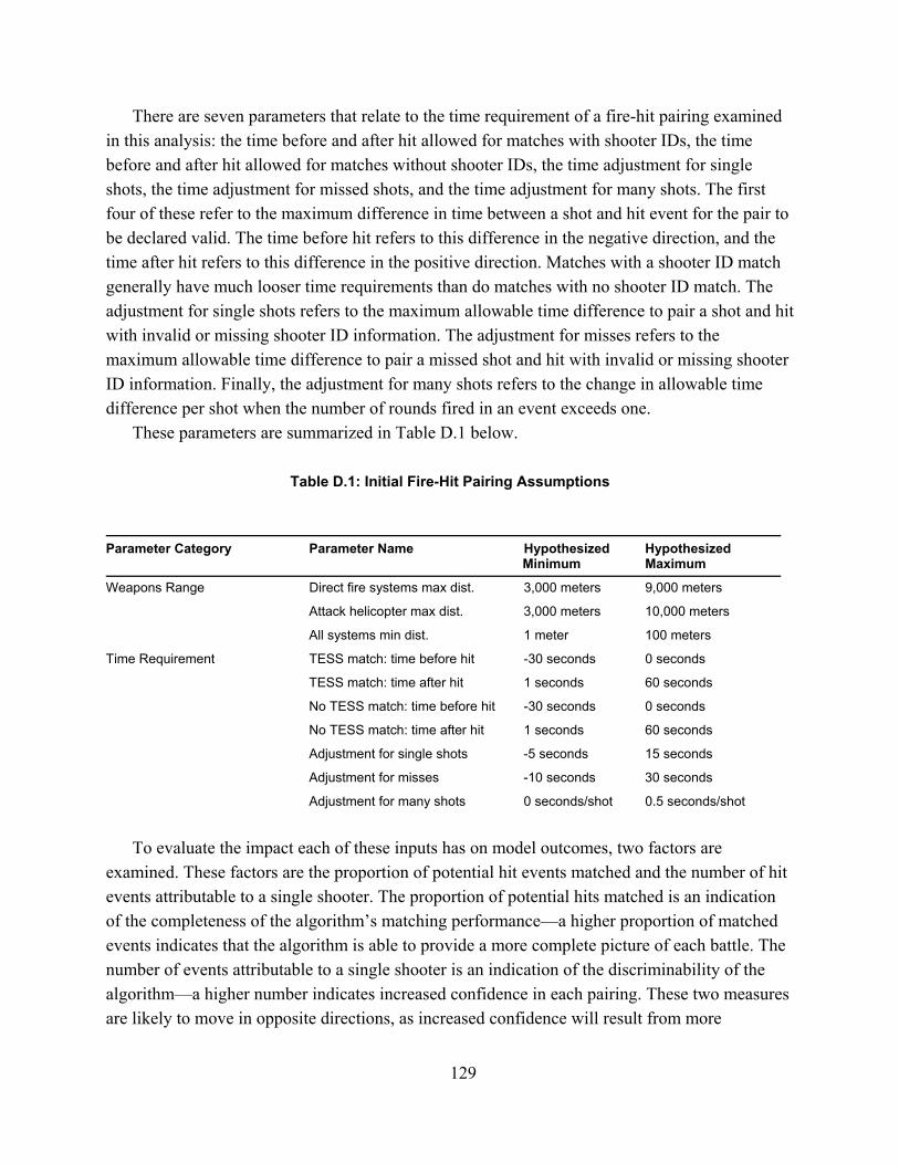
129

There are seven parameters that relate to the time requirement of a fire-hit pairing examined in this analysis: the time before and after hit allowed for matches with shooter IDs, the time before and after hit allowed for matches without shooter IDs, the time adjustment for single shots, the time adjustment for missed shots, and the time adjustment for many shots. The first four of these refer to the maximum difference in time between a shot and hit event for the pair to be declared valid. The time before hit refers to this difference in the negative direction, and the time after hit refers to this difference in the positive direction. Matches with a shooter ID match generally have much looser time requirements than do matches with no shooter ID match. The adjustment for single shots refers to the maximum allowable time difference to pair a shot and hit with invalid or missing shooter ID information. The adjustment for misses refers to the maximum allowable time difference to pair a missed shot and hit with invalid or missing shooter ID information. Finally, the adjustment for many shots refers to the change in allowable time difference per shot when the number of rounds fired in an event exceeds one.

These parameters are summarized in Table D.1 below.

Table D.1: Initial Fire-Hit Pairing Assumptions

Parameter Category Parameter Name Hypothesized Minimum

Hypothesized Maximum

Weapons Range Direct fire systems max dist. 3,000 meters 9,000 meters

Attack helicopter max dist. 3,000 meters 10,000 meters

All systems min dist. 1 meter 100 meters

Time Requirement TESS match: time before hit -30 seconds 0 seconds

TESS match: time after hit 1 seconds 60 seconds

No TESS match: time before hit -30 seconds 0 seconds

No TESS match: time after hit 1 seconds 60 seconds

Adjustment for single shots -5 seconds 15 seconds

Adjustment for misses -10 seconds 30 seconds

Adjustment for many shots 0 seconds/shot 0.5 seconds/shot

To evaluate the impact each of these inputs has on model outcomes, two factors are

examined. These factors are the proportion of potential hit events matched and the number of hit events attributable to a single shooter. The proportion of potential hits matched is an indication of the completeness of the algorithm’s matching performance—a higher proportion of matched events indicates that the algorithm is able to provide a more complete picture of each battle. The number of events attributable to a single shooter is an indication of the discriminability of the algorithm—a higher number indicates increased confidence in each pairing. These two measures are likely to move in opposite directions, as increased confidence will result from more

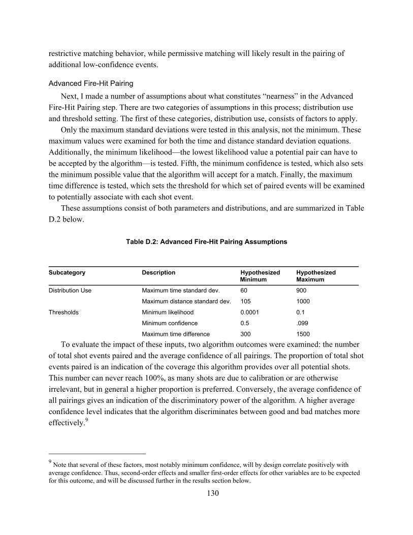
130

restrictive matching behavior, while permissive matching will likely result in the pairing of additional low-confidence events.

Advanced Fire-Hit Pairing

Next, I made a number of assumptions about what constitutes “nearness” in the Advanced Fire-Hit Pairing step. There are two categories of assumptions in this process; distribution use and threshold setting. The first of these categories, distribution use, consists of factors to apply.

Only the maximum standard deviations were tested in this analysis, not the minimum. These maximum values were examined for both the time and distance standard deviation equations. Additionally, the minimum likelihood—the lowest likelihood value a potential pair can have to be accepted by the algorithm—is tested. Fifth, the minimum confidence is tested, which also sets the minimum possible value that the algorithm will accept for a match. Finally, the maximum time difference is tested, which sets the threshold for which set of paired events will be examined to potentially associate with each shot event.

These assumptions consist of both parameters and distributions, and are summarized in Table D.2 below.

Table D.2: Advanced Fire-Hit Pairing Assumptions

Subcategory Description Hypothesized Minimum

Hypothesized Maximum

Distribution Use

Maximum time standard dev. 60 900

Maximum distance standard dev. 105 1000

Thresholds Minimum likelihood 0.0001 0.1

Minimum confidence 0.5 .099

Maximum time difference 300 1500

To evaluate the impact of these inputs, two algorithm outcomes were examined: the number of total shot events paired and the average confidence of all pairings. The proportion of total shot events paired is an indication of the coverage this algorithm provides over all potential shots. This number can never reach 100%, as many shots are due to calibration or are otherwise irrelevant, but in general a higher proportion is preferred. Conversely, the average confidence of all pairings gives an indication of the discriminatory power of the algorithm. A higher average confidence level indicates that the algorithm discriminates between good and bad matches more effectively.9

9 Note that several of these factors, most notably minimum confidence, will by design correlate positively with average confidence. Thus, second-order effects and smaller first-order effects for other variables are to be expected for this outcome, and will be discussed further in the results section below.

131

Contact Creation

The third set of assumptions focus on what constitutes a “contact” and are used in the Contact Creation step. There are three parameters tested in this process, each relating to the distance threshold for one entity or unit to be considered a member of a unit or contact. The first of these is company-level convex hull distance, which describes the maximum allowable distance outside the convex hull formed by entities in a company in contact for a weapon system to be considered part of that company in that contact. The second, battalion-level convex hull distance, describes the analogous distance for a weapon system to be considered part of a battalion. The third, mean distance threshold, describes the threshold for a fire-hit pair’s locations to be included in that of a contact. If the candidate locations in a fire-hit pair have a standard deviation greater than this threshold, the shooting entity locations from that event are not added to the contact (though the event itself is added).10 These assumptions consist of thresholds and parameters, and are summarized in Table D.3 below.

Table D.3: Contact Creation Assumptions

Subcategory Description Hypothesized Minimum

Hypothesized Maximum

Distance Membership Company-Level convex hull distance

0 1000

Battalion-Level convex hull distance

0 2000

Mean distance threshold 0 500

There are three outcomes that are investigated for the contact creation process: Number of

single shot contacts, average contact area, and average number of events per contact. The number of single shot contacts indicates the number of contacts created throughout a rotation that contain only a single fire-hit pair. This outcome gives an indication of the algorithm’s effectiveness at merging contacts together, when appropriate. The average contact area describes the average area, measured by the convex hull of all weapon system locations over the duration of the contact, of all contacts in a rotation. The average number of events per contact indicates the average number of fire-hit pairs in each contact, over all contacts in a rotation. Moderate values of these two outcomes indicate that the algorithm was effective at both merging contacts together as well as not excessively merging contacts.

10 This restriction ensures highly uncertain locations are not used in contact merging or event joining calculations.

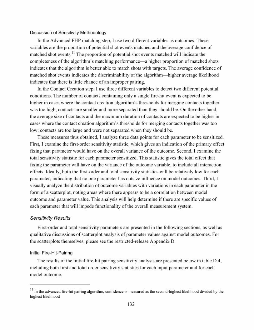
132

Discussion of Sensitivity Methodology

In the Advanced FHP matching step, I use two different variables as outcomes. These variables are the proportion of potential shot events matched and the average confidence of matched shot events.11 The proportion of potential shot events matched will indicate the completeness of the algorithm’s matching performance—a higher proportion of matched shots indicates that the algorithm is better able to match shots with targets. The average confidence of matched shot events indicates the discriminability of the algorithm—higher average likelihood indicates that there is little chance of an improper pairing.

In the Contact Creation step, I use three different variables to detect two different potential conditions. The number of contacts containing only a single fire-hit event is expected to be higher in cases where the contact creation algorithm’s thresholds for merging contacts together was too high; contacts are smaller and more separated than they should be. On the other hand, the average size of contacts and the maximum duration of contacts are expected to be higher in cases where the contact creation algorithm’s thresholds for merging contacts together was too low; contacts are too large and were not separated when they should be.

These measures thus obtained, I analyze three data points for each parameter to be sensitized. First, I examine the first-order sensitivity statistic, which gives an indication of the primary effect fixing that parameter would have on the overall variance of the outcome. Second, I examine the total sensitivity statistic for each parameter sensitized. This statistic gives the total effect that fixing the parameter will have on the variance of the outcome variable, to include all interaction effects. Ideally, both the first-order and total sensitivity statistics will be relatively low for each parameter, indicating that no one parameter has outsize influence on model outcomes. Third, I visually analyze the distribution of outcome variables with variations in each parameter in the form of a scatterplot, noting areas where there appears to be a correlation between model outcome and parameter value. This analysis will help determine if there are specific values of each parameter that will impede functionality of the overall measurement system.

Sensitivity Results

First-order and total sensitivity parameters are presented in the following sections, as well as qualitative discussions of scatterplot analysis of parameter values against model outcomes. For the scatterplots themselves, please see the restricted-release Appendix D.

Initial Fire-Hit-Pairing

The results of the initial fire-hit pairing sensitivity analysis are presented below in table D.4, including both first and total order sensitivity statistics for each input parameter and for each model outcome.

11 In the advanced fire-hit pairing algorithm, confidence is measured as the second-highest likelihood divided by the highest likelihood

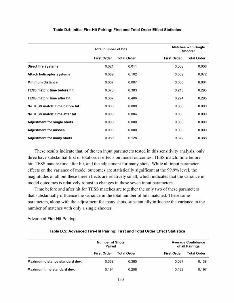
133

Table D.4: Initial Fire-Hit Pairing: First and Total Order Effect Statistics

Total number of hits Matches with Single

Shooter

First Order Total Order First Order Total Order

Direct fire systems 0.021 0.011 0.008 0.006

Attack helicopter systems 0.089 0.102 0.069 0.072

Minimum distance 0.007 0.007 0.006 0.004

TESS match: time before hit 0.373 0.383 0.215 0.293

TESS match: time after hit 0.367 0.406 0.224 0.295

No TESS match: time before hit 0.000 0.000 0.000 0.000

No TESS match: time after hit 0.003 0.004 0.000 0.000

Adjustment for single shots 0.000 0.000 0.000 0.000

Adjustment for misses 0.000 0.000 0.000 0.000

Adjustment for many shots 0.088 0.128 0.372 0.388

These results indicate that, of the ten input parameters tested in this sensitivity analysis, only

three have substantial first or total order effects on model outcomes: TESS match: time before hit, TESS match: time after hit, and the adjustment for many shots. While all input parameter effects on the variance of model outcomes are statistically significant at the 99.9% level, the magnitudes of all but these three effects are relatively small, which indicates that the variance in model outcomes is relatively robust to changes in these seven input parameters.

Time before and after hit for TESS matches are together the only two of these parameters that substantially influence the variance in the total number of hits matched. These same parameters, along with the adjustment for many shots, substantially influence the variance in the number of matches with only a single shooter.

Advanced Fire-Hit Pairing

Table D.5: Advanced Fire-Hit Pairing: First and Total Order Effect Statistics

Number of Shots Paired

Average Confidence

of all Pairings

First Order Total Order First Order Total Order

Maximum distance standard dev. 0.338 0.360 0.067 0.138

Maximum time standard dev. 0.194 0.206 0.122 0.197

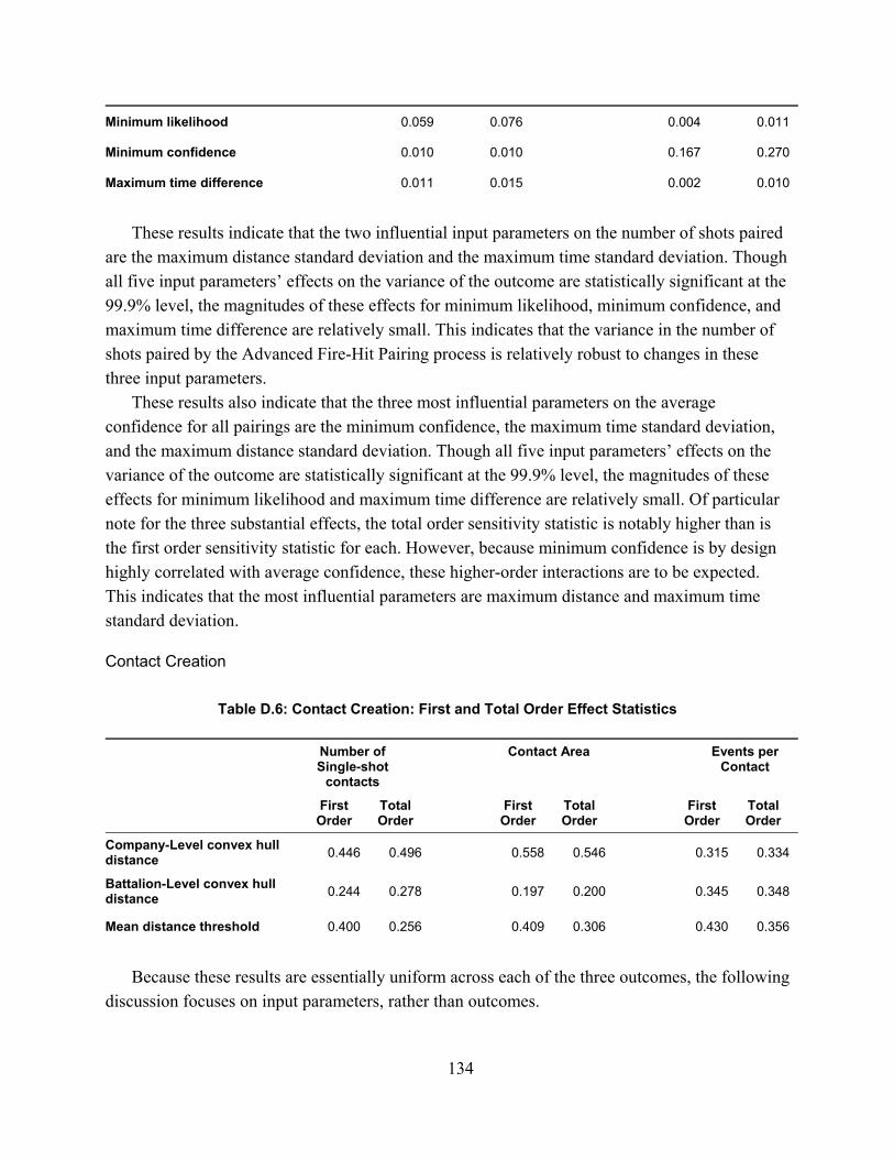
134

Minimum likelihood 0.059 0.076 0.004 0.011

Minimum confidence 0.010 0.010 0.167 0.270

Maximum time difference 0.011 0.015 0.002 0.010

These results indicate that the two influential input parameters on the number of shots paired

are the maximum distance standard deviation and the maximum time standard deviation. Though all five input parameters’ effects on the variance of the outcome are statistically significant at the 99.9% level, the magnitudes of these effects for minimum likelihood, minimum confidence, and maximum time difference are relatively small. This indicates that the variance in the number of shots paired by the Advanced Fire-Hit Pairing process is relatively robust to changes in these three input parameters.

These results also indicate that the three most influential parameters on the average confidence for all pairings are the minimum confidence, the maximum time standard deviation, and the maximum distance standard deviation. Though all five input parameters’ effects on the variance of the outcome are statistically significant at the 99.9% level, the magnitudes of these effects for minimum likelihood and maximum time difference are relatively small. Of particular note for the three substantial effects, the total order sensitivity statistic is notably higher than is the first order sensitivity statistic for each. However, because minimum confidence is by design highly correlated with average confidence, these higher-order interactions are to be expected. This indicates that the most influential parameters are maximum distance and maximum time standard deviation.

Contact Creation

Table D.6: Contact Creation: First and Total Order Effect Statistics

Number of Single-shot

contacts

Contact Area Events per Contact

First Order

Total Order

First Order

Total Order

First Order

Total Order

Company-Level convex hull distance

0.446 0.496 0.558 0.546 0.315 0.334

Battalion-Level convex hull distance

0.244 0.278 0.197 0.200 0.345 0.348

Mean distance threshold 0.400 0.256 0.409 0.306 0.430 0.356

Because these results are essentially uniform across each of the three outcomes, the following

discussion focuses on input parameters, rather than outcomes.

135

The company-level convex hull distance has a considerable effect on model outcomes at extreme ranges of its possible values. When this parameter approaches zero, the average value of all three outcome variables changes substantially; the number of single shot contacts increases, the average contact area decreases markedly, and the number of events per contact drops slightly. These perturbations cease with company-level convex hull distances greater than 250 meters, which is the value this parameter takes on in this dissertation. At extremely high values of this parameter, generally greater than 800 meters, the variance in each model outcome increases. The trend in outcomes at these high levels of company-level convex hull is opposite those at small values of the parameter—the number of single-shot contacts decreases, contact area increases, though the number of events per contact remains essentially unchanged. This indicates that 250 meters is an appropriate value for this parameter.

The battalion-level convex hull distance has a somewhat weaker effect on each model outcome at extreme ranges of its potential values. At extremely small values of this parameter, the number of single-shot contacts increases, the average contact area increases, and the variance in number of events per contact increases without a change in the overall average. These perturbations cease at parameter values greater than 500 meters, which is the value this parameter takes on in this dissertation. There is little to no change in model outcome when this value takes on extremely large values. This indicates that 500 meters is an appropriate value for this parameter.

The mean distance threshold has the weakest effect of the three parameters examined here on model outcomes. However, at extremely small levels of mean distance threshold, outcome values shift in a similar manner to those observed with other parameters in this section. When the mean distance threshold approaches zero, the number of single shot contacts increases, the average contact area dramatically decreases, and the variance in number of events per contact increases. These perturbations cease at parameter values greater than 100 meters, just below the parameter value of 125 meters used in this dissertation.

Computerized model Verification Conclusion

To conclude this portion of the computerized model verification, the overall performance of the model is not solely dependent on any single parameter. While model outcomes do increase in variance with extreme values of each of these parameters, such increases only occurs at values below those used in this analysis.

Operational Validation

The operational validation component of this dissertation consists of an effort to test the validity and reliability of the measures that are extracted from the processed data. In the following paragraphs I describe the methodology for testing the validity and reliability of each of

136

the measures, along with high-level results from validity testing and potential threats to reliability.

Measure Validity Testing Methodology

For the operational validation component of this effort, I conduct an exploratory statistical analysis of each of the measures to be used in JCATS. This analysis seeks to identify the presence or absence of four hypothesized effects on measure outcomes.12 Specifically, I examine four effects: a training effect, and OPFOR effect, a mission type effect, and a “killer” effect. For each effect, observed NTC data is dichotomized according to effect specifications. The differences in means between the two groups are then tested for statistical significance using an approximate permutation test with 10,000 Monte Carlo samples,13 including the P-value correction proposed by Davison and Hinkley (1997).14 Significance levels are indicated by asterisks: one asterisk denotes significance at the 95% level, two asterisks denote significance at the 99% level, and three asterisks denote significance at the 99.9% level.15 Those coefficients significant at the 95% level or greater are discussed in additional detail for each measure. I first explain each of these hypothesized effects before presenting the actual effects observed for each of the measures.

Training effect

The NTC is, as its name suggests, primarily a training institution. Though units undergo a months-long training period to prepare for their NTC rotation, a substantial amount of learning takes place while at the center itself. Oftentimes, the NTC rotation is the first instance in which the entire brigade has maneuvered as a single unit, meaning that some command relationships and communication paths are used for the first time in the early days of each rotation. This lack of practice can lead to significant difficulties as the unit orients itself in both the training environment of the NTC and with its own components. One would expect for these difficulties to

12 For each measure, the observed mean, median, standard deviation, bootstrapped 95% confidence interval,

minimum observed value and maximum observed value are presented in Appendix E. Due to data sensitivity, this Appendix is For Official Use Only and is not releasable to the general public. Please contact the author for access. 13 Andrew S Zieffler, Jeffrey R Harring, and Jeffrey D Long, Comparing Groups: Randomization and Bootstrap Methods Using R (John Wiley & Sons, 2011). 14 Anthony Christopher Davison and David Victor Hinkley, Bootstrap methods and their application, vol. 1 (Cambridge university press, 1997). This correction adds one degree of freedom to the overall model. For a more concise explanation of this correction, see Bernard V North, David Curtis, and Pak C Sham, "A note on the calculation of empirical P values from Monte Carlo procedures," The American Journal of Human Genetics 71, no. 2 (2002). 15 This three-tiered method of hypothesis testing is used throughout this dissertation.

137

peak in the first few days of the rotation and for the unit’s performance to improve as the rotation goes on.16

OPFOR effect

This effect attempts to determine how parameters differ when examining BLUEFOR versus OPFOR units. Because the OPFOR units are based at NTC, they participate in approximately ten rotations per year. This experience means forces are familiar with the terrain and with the environment that they are fighting in. These forces also employ tactics and materiel that are representative of potential adversaries.17 Finally, the goal of the OPFOR is to train the BLUEFOR by exploiting weaknesses, exposing flaws, and fighting with generally little regard for self-preservation. In these regards, they operate in markedly different ways from the BLUEFOR, and one expects these differences to manifest themselves in each measure.

Mission type effect

During each training rotation at NTC, units will engage in a number of distinct missions.18 These missions will vary each rotation, but will generally consist of at least one each of attack, defense, and movement to contact. Though missions and mission types are not directly identified in NTC data, mission types are approximated by examining the magnitude and direction of the aggregate movements in each side during each contact identified. If a given side moved at least 10% of the distance between its center of mass and the enemy’s center of mass,19 that side is marked as “highly mobile.” If the opposing side is not highly mobile, the action is marked as an attack for the mobile side, and a defense for the non-mobile side. If both sides are marked as highly mobile, the action is marked as a “movement to contact.” If neither side is highly mobile, the action type is unknown.20 Each of these mission types requires a different set of planning

16 This effect was noted in Hallmark and Crowley, "Company Performance at the National Training Center: Battle Planning and Execution." 17 Prior to the end of the Cold War, the OPFOR at NTC trained to Soviet Army tactics. Though the present threat is less country-specific, it is still focused on a near-peer threat. "The Soviet Army: Troops, Organization, and Equipment," ed. Headquarters , Department of the Army (Washington, DC1991). 18 Referred to as battle periods by NTC personnel 19 As in other places in this dissertation, center of mass for companies is defined as the geometric median of all component entities in the company. Center of mass for a side is the geometric median of all company centers. 20 These labels are by no means perfect. In particular, movement to contact missions may involve little to no movement on one side (thus looking like an attack/defense to this algorithm), while it is entirely possible for a defensive mission to engage in large spoiling attacks (thus appearing as a movement to contact to this algorithm). Far better would be a qualitative coding of each contact type, followed by a more holistic approach at mission type identification including duration, positions of forces, and more specific movement patterns, possibly employing a machine learning algorithm to categorize these patterns. With that stated however, this measure is intended as a broad look into the existence of a significant mission effect, so the additional accuracy gained by a more complex procedure would only marginally add to this effort. The major effect that one would expect based off this naive coding would be a reduction in overall significance levels, as this effect carries a significant amount of random noise due to measurement error.

138

considerations,21 and units may fight each type in very different ways. One would thus expect unit behaviors to differ based on mission type.

Killer effect

It is recognized by many subject matter experts at the NTC that there is a distinct difference between normal companies and “killer” companies.22 Killer companies are defined as those companies with exceptionally favorable force exchange ratios.23 As force exchange ratio is an outcome variable that captures the great number of skills a unit must master to perform well in combat, units with exceptional exchange ratios will likely differ on other measures from less exemplary units.

Measure Reliability Testing Methodology

From a measurement standpoint, reliability assesses the degree of internal consistency within an item. A simple way of expressing this consistency is in the following equation:

Where Resulti is the measure value for a particular observation, Signali is the unobserved quantity that the measure purports to ascertain, and Errori is some unobserved error in measurement, both random and systemic. A reliable measure will have a relatively high value for Signali and a relatively low value for Errori, while an unreliable measure will have the opposite relationship. In particular, reliable measures will be relatively free from measurement error and uncontrolled third variable effects.

To assess the reliability of the four measures derived in this dissertation then, I qualitatively examine each for the presence of measurement error. I discuss potential solutions for these sources of measurement error when possible. I also qualitatively discuss potential third variable effects on measure outcomes, referencing the results of measure validity testing, when appropriate.

I also quantitatively test the impact of these effects on measure results using a multiple least squares regression. This measure regresses each outcome against effects coded as binary dummy variables, as well as several controls. The exact specifications of each regression differ and will be elaborated for each measure, but all seek to identify overall regression significance, indicating that the variation accounted for by the expected covariates is substantial relative to the

21 As evidenced by the fact that each of these mission types has a separate chapter in most unit doctrinal publications, such as ATP 3-90.1 and FM 3-21.10. Additionally, the confounding nature of mission type was highlighted in Hallmark and Crowley, "Company Performance at the National Training Center: Battle Planning and Execution." 22 Warrior Training Alliance. 23 Here, as in Chapter 4, I define this ratio as that of opposing killed over friendly lost for a given company

139

unexplained variation. This significance is measured in two ways: through the R-squared statistic, and through the overall F or Chi-squared statistic. As the above equation for model validity is directly related to the overall R-squared value for an MLS regression which examines the effect of expected covariates on measure values,24 a high R-squared value indicates a reasonable level of measure reliability. The overall F or chi-squared test for model significance indicates the probability that at least one expected covariate has an effect statistically significantly different from zero. If this statistic is significant, it indicates that at least one of the expected covariates has some explanatory power over the measure. While there is not a single value for either that definitively states whether or not a measure is reliable, the concept of reliability itself is qualitative—at best, one can indicate a satisfying degree of reliability.

Operational Validation Results

Weapon System Probability of Hit

The probability of hit item is calculated over each shot event that has an identifiable target entity. This is a small subset of the total number of shot events that occur in each rotation. However, this subset does allow for a considerable number of covariates to be controlled for when testing validity and reliability. For full results, please see the restricted-release Appendix E.

Measure Validity

To assess the validity of this measure, I test for the presence of the four expected effects: killer, OPFOR, phase, and mission. P-values and significance levels of these effect sizes are presented in an identical manner to other sections, with significance levels of 95% represented with a single asterisk, 99% with two asterisks, and 99.9% with three asterisks.

Prior to testing for measure validity, BMPs are excluded from the dataset. Though data from BMPs and BMP companies appears to be valid for all other measures,25 there are virtually no recorded hits scored by BMPs on BLUEFOR weapon systems. I will not hypothesize as to a cause of this phenomenon, but for the purposes of this measure, and for the JCATS simulation test, will exclude BMP probability of hit data from aggregate calculations.

These significance levels are presented in Table D.7 below.

Table D.7: All non-BMP Companies–Effect Sizes and Significance for Overall Probability of Hit

Effect Name P Value of Difference in Means

24 Robin K Henson, "Understanding Internal Consistency Reliability Estimates: A Conceptual Primer on Coefficient Aalpha," Measurement and Evaluation in Counseling and Development 34, no. 3 (2001). 25 Effects magnitudes and significance levels are in the same range and summary statistics indicate similar central tendency as other weapon systems for rate of fire, unit dispersion, and unit movement speed.

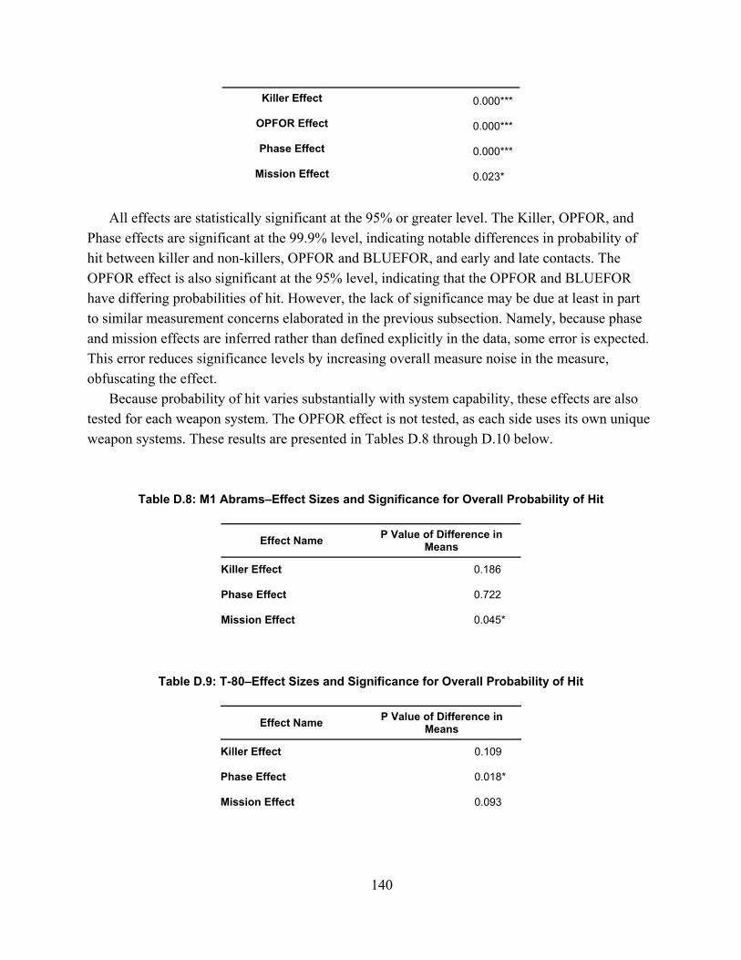
140

Killer Effect 0.000***

OPFOR Effect 0.000***

Phase Effect 0.000***

Mission Effect 0.023***

All effects are statistically significant at the 95% or greater level. The Killer, OPFOR, and

Phase effects are significant at the 99.9% level, indicating notable differences in probability of hit between killer and non-killers, OPFOR and BLUEFOR, and early and late contacts. The OPFOR effect is also significant at the 95% level, indicating that the OPFOR and BLUEFOR have differing probabilities of hit. However, the lack of significance may be due at least in part to similar measurement concerns elaborated in the previous subsection. Namely, because phase and mission effects are inferred rather than defined explicitly in the data, some error is expected. This error reduces significance levels by increasing overall measure noise in the measure, obfuscating the effect.

Because probability of hit varies substantially with system capability, these effects are also tested for each weapon system. The OPFOR effect is not tested, as each side uses its own unique weapon systems. These results are presented in Tables D.8 through D.10 below.

Table D.8: M1 Abrams–Effect Sizes and Significance for Overall Probability of Hit

Effect Name P Value of Difference in

Means

Killer Effect 0.186***

Phase Effect 0.722***

Mission Effect 0.045***

Table D.9: T-80–Effect Sizes and Significance for Overall Probability of Hit

Effect Name P Value of Difference in

Means

Killer Effect 0.109***

Phase Effect 0.018***

Mission Effect 0.093***

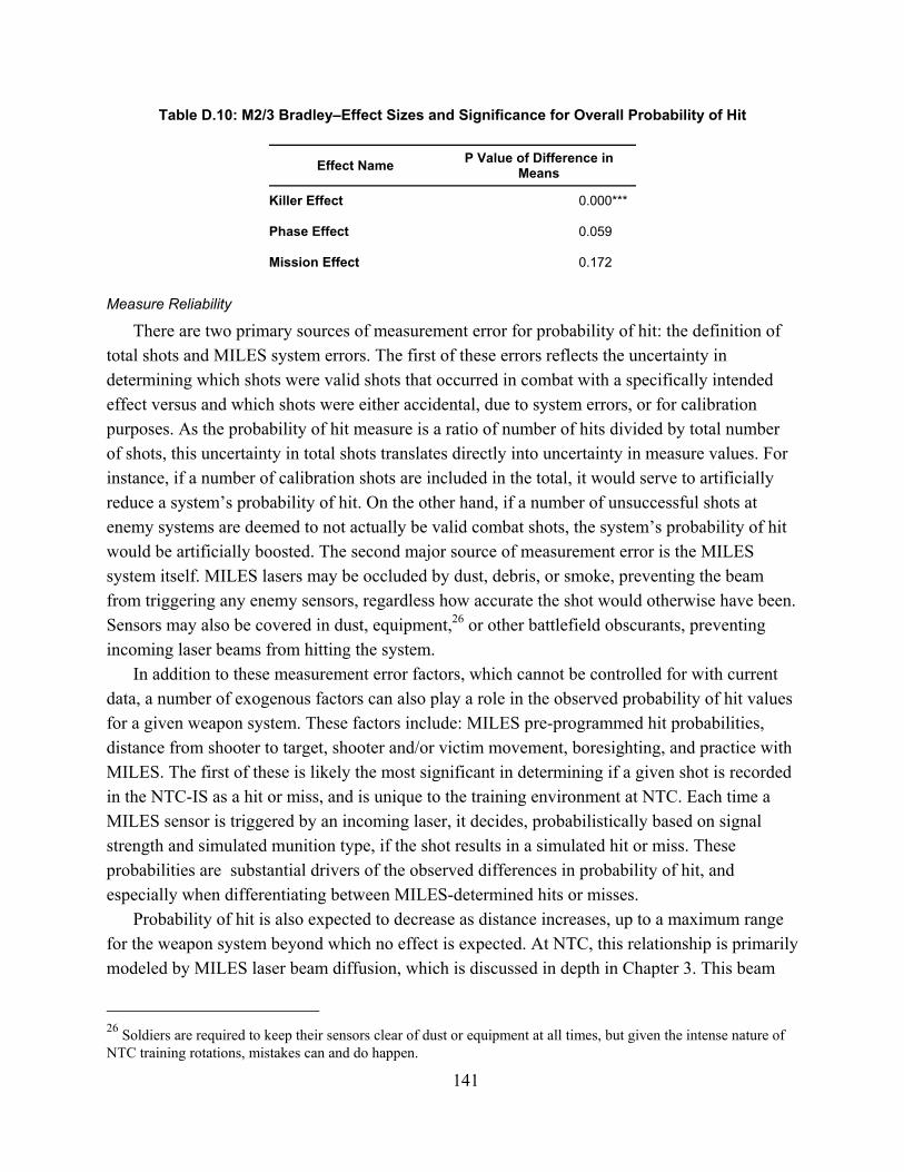
141

Table D.10: M2/3 Bradley–Effect Sizes and Significance for Overall Probability of Hit

Effect Name P Value of Difference in

Means

Killer Effect 0.000***

Phase Effect 0.059***

Mission Effect 0.172***

Measure Reliability

There are two primary sources of measurement error for probability of hit: the definition of total shots and MILES system errors. The first of these errors reflects the uncertainty in determining which shots were valid shots that occurred in combat with a specifically intended effect versus and which shots were either accidental, due to system errors, or for calibration purposes. As the probability of hit measure is a ratio of number of hits divided by total number of shots, this uncertainty in total shots translates directly into uncertainty in measure values. For instance, if a number of calibration shots are included in the total, it would serve to artificially reduce a system’s probability of hit. On the other hand, if a number of unsuccessful shots at enemy systems are deemed to not actually be valid combat shots, the system’s probability of hit would be artificially boosted. The second major source of measurement error is the MILES system itself. MILES lasers may be occluded by dust, debris, or smoke, preventing the beam from triggering any enemy sensors, regardless how accurate the shot would otherwise have been. Sensors may also be covered in dust, equipment,26 or other battlefield obscurants, preventing incoming laser beams from hitting the system.

In addition to these measurement error factors, which cannot be controlled for with current data, a number of exogenous factors can also play a role in the observed probability of hit values for a given weapon system. These factors include: MILES pre-programmed hit probabilities, distance from shooter to target, shooter and/or victim movement, boresighting, and practice with MILES. The first of these is likely the most significant in determining if a given shot is recorded in the NTC-IS as a hit or miss, and is unique to the training environment at NTC. Each time a MILES sensor is triggered by an incoming laser, it decides, probabilistically based on signal strength and simulated munition type, if the shot results in a simulated hit or miss. These probabilities are substantial drivers of the observed differences in probability of hit, and especially when differentiating between MILES-determined hits or misses.

Probability of hit is also expected to decrease as distance increases, up to a maximum range for the weapon system beyond which no effect is expected. At NTC, this relationship is primarily modeled by MILES laser beam diffusion, which is discussed in depth in Chapter 3. This beam

26 Soldiers are required to keep their sensors clear of dust or equipment at all times, but given the intense nature of NTC training rotations, mistakes can and do happen.

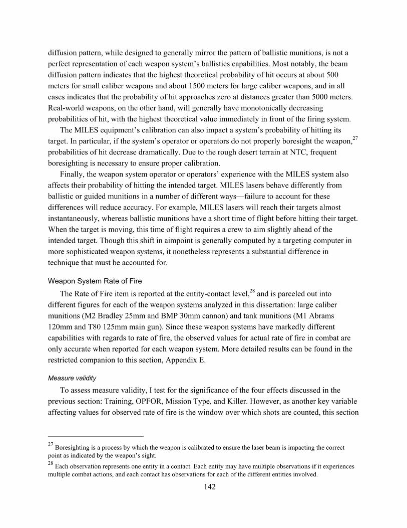
142

diffusion pattern, while designed to generally mirror the pattern of ballistic munitions, is not a perfect representation of each weapon system’s ballistics capabilities. Most notably, the beam diffusion pattern indicates that the highest theoretical probability of hit occurs at about 500 meters for small caliber weapons and about 1500 meters for large caliber weapons, and in all cases indicates that the probability of hit approaches zero at distances greater than 5000 meters. Real-world weapons, on the other hand, will generally have monotonically decreasing probabilities of hit, with the highest theoretical value immediately in front of the firing system.

The MILES equipment’s calibration can also impact a system’s probability of hitting its target. In particular, if the system’s operator or operators do not properly boresight the weapon,27 probabilities of hit decrease dramatically. Due to the rough desert terrain at NTC, frequent boresighting is necessary to ensure proper calibration.

Finally, the weapon system operator or operators’ experience with the MILES system also affects their probability of hitting the intended target. MILES lasers behave differently from ballistic or guided munitions in a number of different ways—failure to account for these differences will reduce accuracy. For example, MILES lasers will reach their targets almost instantaneously, whereas ballistic munitions have a short time of flight before hitting their target. When the target is moving, this time of flight requires a crew to aim slightly ahead of the intended target. Though this shift in aimpoint is generally computed by a targeting computer in more sophisticated weapon systems, it nonetheless represents a substantial difference in technique that must be accounted for.

Weapon System Rate of Fire

The Rate of Fire item is reported at the entity-contact level,28 and is parceled out into different figures for each of the weapon systems analyzed in this dissertation: large caliber munitions (M2 Bradley 25mm and BMP 30mm cannon) and tank munitions (M1 Abrams 120mm and T80 125mm main gun). Since these weapon systems have markedly different capabilities with regards to rate of fire, the observed values for actual rate of fire in combat are only accurate when reported for each weapon system. More detailed results can be found in the restricted companion to this section, Appendix E.

Measure validity

To assess measure validity, I test for the significance of the four effects discussed in the previous section: Training, OPFOR, Mission Type, and Killer. However, as another key variable affecting values for observed rate of fire is the window over which shots are counted, this section

27 Boresighting is a process by which the weapon is calibrated to ensure the laser beam is impacting the correct point as indicated by the weapon’s sight. 28 Each observation represents one entity in a contact. Each entity may have multiple observations if it experiences multiple combat actions, and each contact has observations for each of the different entities involved.

143

also examines how each of these effects varies with changes in the time span over which this measure is calculated.

In Appendix E,29 summary statistics and histograms of observed values are presented for the interested reader, as well as detailed charts highlighting effects over different window sizes. Included below are effect sizes for each of the four main effects analyzed in this dissertation, broken out by weapon system.

Table D.12: Tanks—Effect Sizes and Significance for Rate of Fire

Effect Name P Value of Difference in Means

Killer Effect 0.006*** 

OPFOR Effect 0.000*** 

Phase Effect 0.530*** 

Mission Effect 0.300*** 

Table D.13: IFVs—Effect Sizes and Significance for Rate of Fire

Effect Name P Value of Difference inMeans

Killer Effect 0.000*** 

OPFOR Effect 0.000*** 

Phase Effect 0.072*** 

Mission Effect 0.536*** 

These results indicate a favorable degree of measure validity. In particular, the strong

significance of the OPFOR and Killer effects indicate a promising degree of differentiability for this measure. The lack of significance for the Phase and Mission effects is not ideal, but the measurement error for both of these effects (discussed in the previous section) is likely a substantial factor in reducing effect sizes. It is also possible that actual rates of fire do not, in fact, change with changes in phase and mission type.

These effects do vary somewhat when the window duration is adjusted. Expanding this window will almost always reduce the observed rate of fire, as direct fire entities tend to shoot in

29 Appendix E is release-restricted due to data sensitivity. Please contact the author for access.

144

short bursts punctuated by long pauses, rather than constant rates throughout an entire contact. For much of this research, 20 seconds is used as a window duration, as it is longer than the reload time for any munition, but is still short enough to produce significant variation between entities’ observed rates. However, when examining each of the effects presented in the following subsection, a multitude of other window sizes were also examined, from 1 to 1000 seconds. Each of the effects described persists with most of these different window sizes, indicating that comparative effects are robust to window size.

The Killer effect is most pronounced at larger window sizes: The difference in mean rates of fire between killer companies and non-killer companies becomes insignificant (at the 95% level) at window durations less than 14 seconds for tanks and 2 seconds for IFVs. The OPFOR effect also varies substantially with window duration. For tanks, OPFOR fires at a faster rate (at the 95% level) for windows only between 5 and 30 seconds. For IFVs, BLUEFOR shoots at a faster rate for short windows (1 to 3 seconds) while OPFOR shoots at a faster rate for longer windows (8 seconds and longer). This latter pattern suggests BLUEFOR IFVs tend to shoot in short bursts, while OPFOR IFVs tend to shoot in a more sustained manner. The Phase and Mission effects are not significant (at the 95% level) for any window duration between 1 and 1000 seconds for either tanks or IFVs.

Measure reliability

There are four main sources of measurement error in this measure. The first comes from potential errors in the grouping of shots into contacts. As this measure is aggregated at the entity-contact level, the correct definition of contacts is important in ensuring shots are counted in an appropriate manner. If contacts are excessively aggregated, the measure value will be inflated, while if contacts are incorrectly separated, the measure value will be artificially reduced. The second source of measurement error is the classification of contacts as boresighting or non-boresighting contacts. During calculation of this measure, events flagged as boresighting or otherwise non-combat related are removed under the assumption that those values do not adequately represent a physical contact situation. However, the algorithms to detect boresighting contacts are not perfect; misclassification of regular contacts as boresighting and vice versa may introduce additional random error into measure values. The MILES system itself is a third source of measurement error. The MILES transmission system can mis-handle incoming shot event data, resulting in those events being dropped from the database. The transmission system can also duplicate incoming data streams, either due to faults in the laser receiver on the target vehicle or to faults in the radio transmitter signal. Finally, this measure only uses shot events that were matched to a target unit or entity in order to reduce the number of irrelevant shot events composing the measure.30 Though these shot events compose the majority of shots that occurred

30These events include shots that hit the target as well as those that missed, but were picked up by the MILES system, and those that missed, but occurred near enough to other shots such that the target could be inferred through

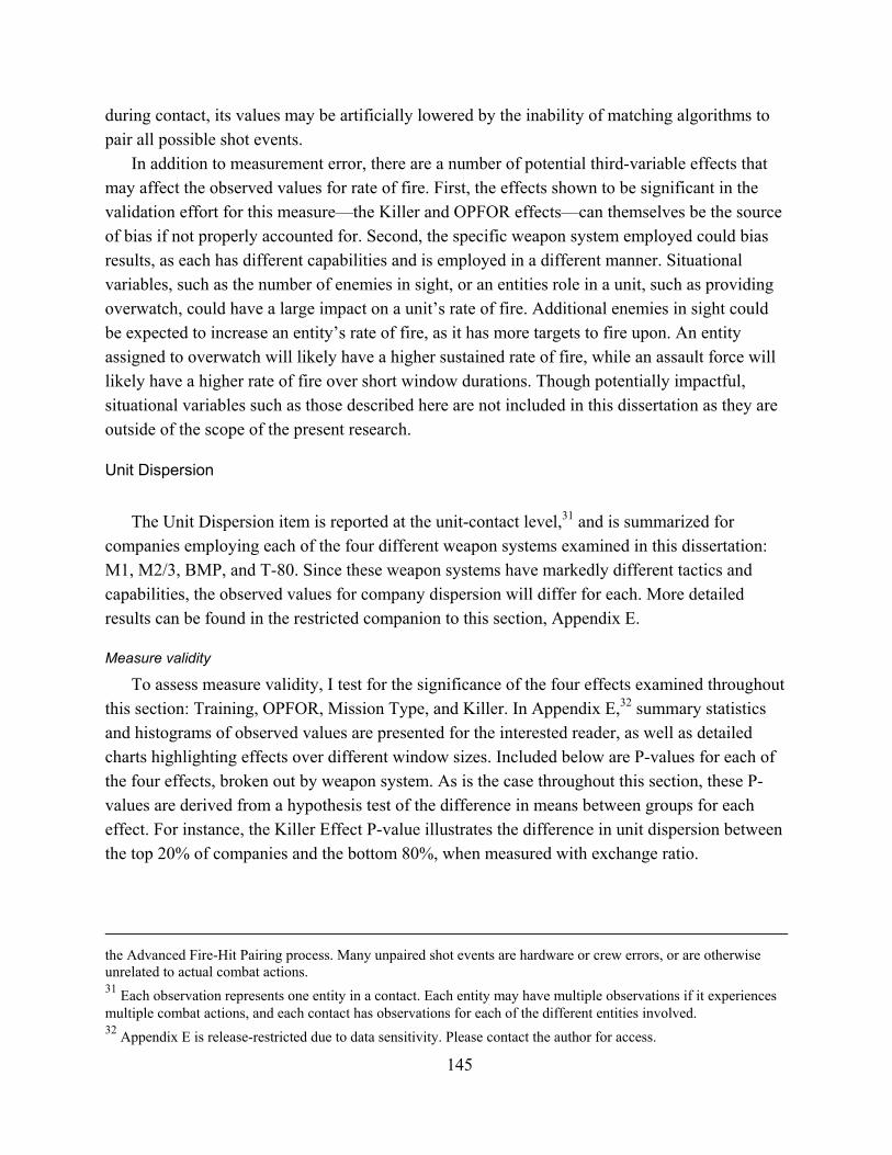
145

during contact, its values may be artificially lowered by the inability of matching algorithms to pair all possible shot events.

In addition to measurement error, there are a number of potential third-variable effects that may affect the observed values for rate of fire. First, the effects shown to be significant in the validation effort for this measure—the Killer and OPFOR effects—can themselves be the source of bias if not properly accounted for. Second, the specific weapon system employed could bias results, as each has different capabilities and is employed in a different manner. Situational variables, such as the number of enemies in sight, or an entities role in a unit, such as providing overwatch, could have a large impact on a unit’s rate of fire. Additional enemies in sight could be expected to increase an entity’s rate of fire, as it has more targets to fire upon. An entity assigned to overwatch will likely have a higher sustained rate of fire, while an assault force will likely have a higher rate of fire over short window durations. Though potentially impactful, situational variables such as those described here are not included in this dissertation as they are outside of the scope of the present research.

Unit Dispersion

The Unit Dispersion item is reported at the unit-contact level,31 and is summarized for

companies employing each of the four different weapon systems examined in this dissertation: M1, M2/3, BMP, and T-80. Since these weapon systems have markedly different tactics and capabilities, the observed values for company dispersion will differ for each. More detailed results can be found in the restricted companion to this section, Appendix E.

Measure validity

To assess measure validity, I test for the significance of the four effects examined throughout this section: Training, OPFOR, Mission Type, and Killer. In Appendix E,32 summary statistics and histograms of observed values are presented for the interested reader, as well as detailed charts highlighting effects over different window sizes. Included below are P-values for each of the four effects, broken out by weapon system. As is the case throughout this section, these P-values are derived from a hypothesis test of the difference in means between groups for each effect. For instance, the Killer Effect P-value illustrates the difference in unit dispersion between the top 20% of companies and the bottom 80%, when measured with exchange ratio.

the Advanced Fire-Hit Pairing process. Many unpaired shot events are hardware or crew errors, or are otherwise unrelated to actual combat actions. 31 Each observation represents one entity in a contact. Each entity may have multiple observations if it experiences multiple combat actions, and each contact has observations for each of the different entities involved. 32 Appendix E is release-restricted due to data sensitivity. Please contact the author for access.

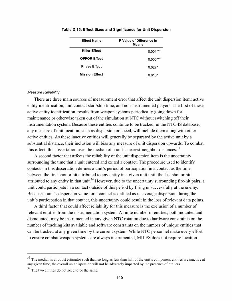
146

Table D.15: Effect Sizes and Significance for Unit Dispersion

Effect Name P Value of Difference in Means

Killer Effect 0.001***

OPFOR Effect 0.000***

Phase Effect 0.027***

Mission Effect 0.016***

Measure Reliability

There are three main sources of measurement error that affect the unit dispersion item: active entity identification, unit contact start/stop time, and non-instrumented players. The first of these, active entity identification, results from weapon systems periodically going down for maintenance or otherwise taken out of the simulation at NTC without switching off their instrumentation system. Because these entities continue to be tracked, in the NTC-IS database, any measure of unit location, such as dispersion or speed, will include them along with other active entities. As these inactive entities will generally be separated by the active unit by a substantial distance, their inclusion will bias any measure of unit dispersion upwards. To combat this effect, this dissertation uses the median of a unit’s nearest-neighbor distances.33

A second factor that affects the reliability of the unit dispersion item is the uncertainty surrounding the time that a unit entered and exited a contact. The procedure used to identify contacts in this dissertation defines a unit’s period of participation in a contact as the time between the first shot or hit attributed to any entity in a given unit until the last shot or hit attributed to any entity in that unit.34 However, due to the uncertainty surrounding fire-hit pairs, a unit could participate in a contact outside of this period by firing unsuccessfully at the enemy. Because a unit’s dispersion value for a contact is defined as its average dispersion during the unit’s participation in that contact, this uncertainty could result in the loss of relevant data points.

A third factor that could affect reliability for this measure is the exclusion of a number of relevant entities from the instrumentation system. A finite number of entities, both mounted and dismounted, may be instrumented in any given NTC rotation due to hardware constraints on the number of tracking kits available and software constraints on the number of unique entities that can be tracked at any given time by the current system. While NTC personnel make every effort to ensure combat weapon systems are always instrumented, MILES does not require location

33 The median is a robust estimator such that, so long as less than half of the unit’s component entities are inactive at any given time, the overall unit dispersion will not be adversely impacted by the presence of outliers. 34 The two entities do not need to be the same.

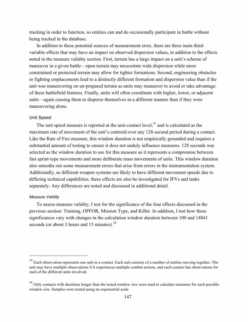
147

tracking in order to function, so entities can and do occasionally participate in battle without being tracked in the database.

In addition to these potential sources of measurement error, there are three main third-variable effects that may have an impact on observed dispersion values, in addition to the effects noted in the measure validity section. First, terrain has a large impact on a unit’s scheme of maneuver in a given battle—open terrain may necessitate wide dispersion while more constrained or protected terrain may allow for tighter formations. Second, engineering obstacles or fighting emplacements lead to a distinctly different formation and dispersion value than if the unit was maneuvering on un-prepared terrain as units may maneuver to avoid or take advantage of these battlefield features. Finally, units will often coordinate with higher, lower, or adjacent units—again causing them to disperse themselves in a different manner than if they were maneuvering alone.

Unit Speed

The unit speed measure is reported at the unit-contact level,35 and is calculated as the maximum rate of movement of the unit’s centroid over any 128-second period during a contact. Like the Rate of Fire measure, this window duration is not empirically grounded and requires a substantial amount of testing to ensure it does not unduly influence measures. 128 seconds was selected as the window duration to use for this measure as it represents a compromise between fast sprint-type movements and more deliberate mass movements of units. This window duration also smooths out some measurement errors that arise from errors in the instrumentation system. Additionally, as different weapon systems are likely to have different movement speeds due to differing technical capabilities, these effects are also be investigated for IFVs and tanks separately. Any differences are noted and discussed in additional detail.

Measure Validity

To assess measure validity, I test for the significance of the four effects discussed in the previous section: Training, OPFOR, Mission Type, and Killer. In addition, I test how these significances vary with changes in the calculation window duration between 100 and 14841 seconds (or about 3 hours and 15 minutes).36

35 Each observation represents one unit in a contact. Each unit consists of a number of entities moving together. The unit may have multiple observations if it experiences multiple combat actions, and each contact has observations for each of the different units involved.

36 Only contacts with durations longer than the tested window size were used to calculate measures for each possible window size. Samples were tested using an exponential scale

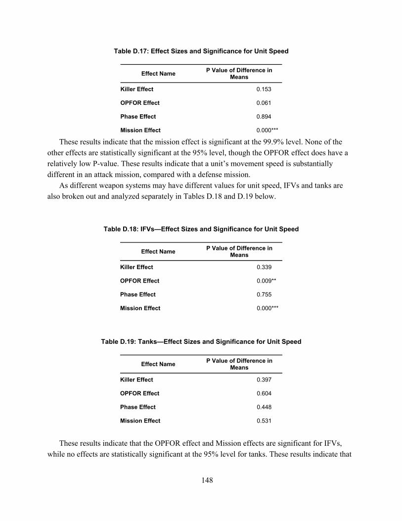
148

Table D.17: Effect Sizes and Significance for Unit Speed

Effect Name P Value of Difference in

Means

Killer Effect 0.153***

OPFOR Effect 0.061***

Phase Effect 0.894***

Mission Effect 0.000***

These results indicate that the mission effect is significant at the 99.9% level. None of the other effects are statistically significant at the 95% level, though the OPFOR effect does have a relatively low P-value. These results indicate that a unit’s movement speed is substantially different in an attack mission, compared with a defense mission.

As different weapon systems may have different values for unit speed, IFVs and tanks are also broken out and analyzed separately in Tables D.18 and D.19 below.

Table D.18: IFVs—Effect Sizes and Significance for Unit Speed

Effect Name P Value of Difference in

Means

Killer Effect 0.339***

OPFOR Effect 0.009***

Phase Effect 0.755***

Mission Effect 0.000***

Table D.19: Tanks—Effect Sizes and Significance for Unit Speed

Effect Name P Value of Difference in

Means

Killer Effect 0.397***

OPFOR Effect 0.604***

Phase Effect 0.448***

Mission Effect 0.531***

These results indicate that the OPFOR effect and Mission effects are significant for IFVs,

while no effects are statistically significant at the 95% level for tanks. These results indicate that

149

there is substantially more uncertainty in tank movement speeds than there is in IFV movement speeds, as indicated by relationships with expected effects.

When the window over which this measure is calculated is varied, these effects largely remain the same. Below in Figures D.2 through D.4 are plots of the P-values of the difference in means for each effect over each of the three populations examined here—all weapons, only tanks, and only IFVs. These graphs are each truncated at P-values of 0.2 for readability, and include a red line indicating the 95% significance level.

Figure D.2: Significance levels with varying window duration: all weapon systems

Figure D.3: Significance levels with varying window duration: Tanks

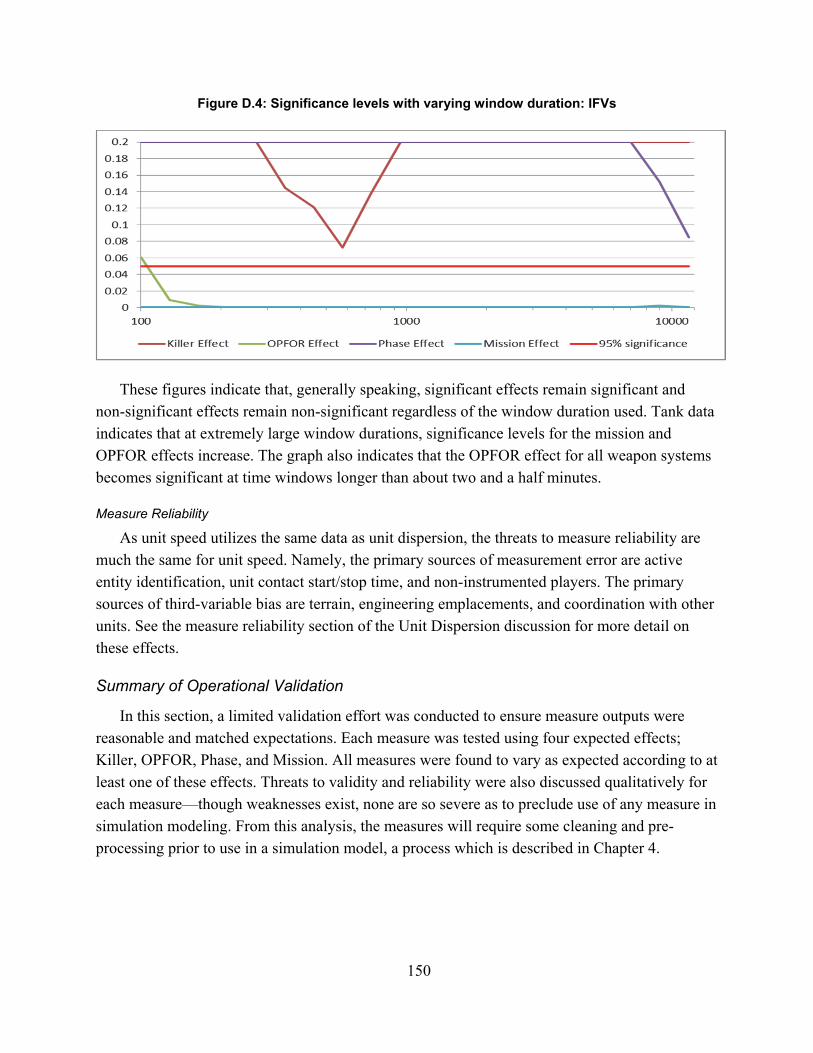
150

Figure D.4: Significance levels with varying window duration: IFVs

These figures indicate that, generally speaking, significant effects remain significant and non-significant effects remain non-significant regardless of the window duration used. Tank data indicates that at extremely large window durations, significance levels for the mission and OPFOR effects increase. The graph also indicates that the OPFOR effect for all weapon systems becomes significant at time windows longer than about two and a half minutes.

Measure Reliability

As unit speed utilizes the same data as unit dispersion, the threats to measure reliability are much the same for unit speed. Namely, the primary sources of measurement error are active entity identification, unit contact start/stop time, and non-instrumented players. The primary sources of third-variable bias are terrain, engineering emplacements, and coordination with other units. See the measure reliability section of the Unit Dispersion discussion for more detail on these effects.

Summary of Operational Validation

In this section, a limited validation effort was conducted to ensure measure outputs were reasonable and matched expectations. Each measure was tested using four expected effects; Killer, OPFOR, Phase, and Mission. All measures were found to vary as expected according to at least one of these effects. Threats to validity and reliability were also discussed qualitatively for each measure—though weaknesses exist, none are so severe as to preclude use of any measure in simulation modeling. From this analysis, the measures will require some cleaning and pre-processing prior to use in a simulation model, a process which is described in Chapter 4.

151

Appendix E: Full Results of NTC-IS Analysis

This appendix is For Official Use Only and is thus not available to the general public. Please contact the RAND Arroyo Center to request access.

152

Appendix F: Regression Model Specifications and Diagnostics

Experimental Design Matrices

Table F.1: Design A Data Matrix

Data Source

Scenario Name

Data Source

Mission Enemy Terrain Mission & Data

Source

Enemy & Data

Source

Terrain & Data

Source

Curvature

Baseline Base 0 0 0 0 0 0 0 1

Baseline Bottom Left

0 -1 -1 -1 0 0 0 0

Baseline Bottom Right

0 1 -1 1 0 0 0 0

Baseline Top Left 0 1 1 -1 0 0 0 0

Baseline Top Right 0 -1 1 1 0 0 0 0

NTC Base 1 0 0 0 0 0 0 1

NTC Bottom Left

1 -1 -1 -1 -1 -1 -1 0

NTC Bottom Right

1 1 -1 1 1 -1 1 0

NTC Top Left 1 1 1 -1 1 1 -1 0

NTC Top Right 1 -1 1 1 -1 1 1 0

Table F.2: Design B Data Matrix

Side Data Source

Scenario Name

Data Source

Side Side & Data

Source

Mission Enemy Terrain Mission & Data Source

Enemy & Data Source

BLUEFOR Baseline Base 0 0 0 0 0 0 0 0

BLUEFOR Baseline Bottom Left

0 0 0 -1 -1 -1 0 0

BLUEFOR Baseline Bottom Right

0 0 0 1 -1 1 0 0

BLUEFOR Baseline Top Left 0 0 0 1 1 -1 0 0

BLUEFOR Baseline Top Right 0 0 0 -1 1 1 0 0

BLUEFOR NTC Base 1 0 0 0 0 0 0 0

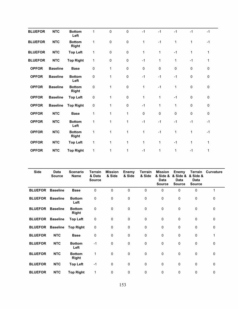
153

BLUEFOR NTC Bottom Left

1 0 0 -1 -1 -1 -1 -1

BLUEFOR NTC Bottom Right

1 0 0 1 -1 1 1 -1

BLUEFOR NTC Top Left 1 0 0 1 1 -1 1 1

BLUEFOR NTC Top Right 1 0 0 -1 1 1 -1 1

OPFOR Baseline Base 0 1 0 0 0 0 0 0

OPFOR Baseline Bottom Left

0 1 0 -1 -1 -1 0 0

OPFOR Baseline Bottom Right

0 1 0 1 -1 1 0 0

OPFOR Baseline Top Left 0 1 0 1 1 -1 0 0

OPFOR Baseline Top Right 0 1 0 -1 1 1 0 0

OPFOR NTC Base 1 1 1 0 0 0 0 0

OPFOR NTC Bottom Left

1 1 1 -1 -1 -1 -1 -1

OPFOR NTC Bottom Right

1 1 1 1 -1 1 1 -1

OPFOR NTC Top Left 1 1 1 1 1 -1 1 1

OPFOR NTC Top Right 1 1 1 -1 1 1 -1 1

Side Data Source

Scenario Name

Terrain & Data Source

Mission & Side

Enemy & Side

Terrain & Side

Mission & Side &

Data Source

Enemy & Side &

Data Source

Terrain & Side &

Data Source

Curvature

BLUEFOR Baseline Base 0 0 0 0 0 0 0 1

BLUEFOR Baseline Bottom Left

0 0 0 0 0 0 0 0

BLUEFOR Baseline Bottom Right

0 0 0 0 0 0 0 0

BLUEFOR Baseline Top Left 0 0 0 0 0 0 0 0

BLUEFOR Baseline Top Right 0 0 0 0 0 0 0 0

BLUEFOR NTC Base 0 0 0 0 0 0 0 1

BLUEFOR NTC Bottom Left

-1 0 0 0 0 0 0 0

BLUEFOR NTC Bottom Right

1 0 0 0 0 0 0 0

BLUEFOR NTC Top Left -1 0 0 0 0 0 0 0

BLUEFOR NTC Top Right 1 0 0 0 0 0 0 0

154

OPFOR Baseline Base 0 0 0 0 0 0 0 1

OPFOR Baseline Bottom Left

0 -1 -1 -1 0 0 0 0

OPFOR Baseline Bottom Right

0 1 -1 1 0 0 0 0

OPFOR Baseline Top Left 0 1 1 -1 0 0 0 0

OPFOR Baseline Top Right 0 -1 1 1 0 0 0 0

OPFOR NTC Base 0 0 0 0 0 0 0 1

OPFOR NTC Bottom Left

-1 -1 -1 -1 -1 -1 -1 0

OPFOR NTC Bottom Right

1 1 -1 1 1 -1 1 0

OPFOR NTC Top Left -1 1 1 -1 1 1 -1 0

OPFOR NTC Top Right 1 -1 1 1 -1 1 1 0

Regression Equations

Design A

_

_

_

_

Design B

_

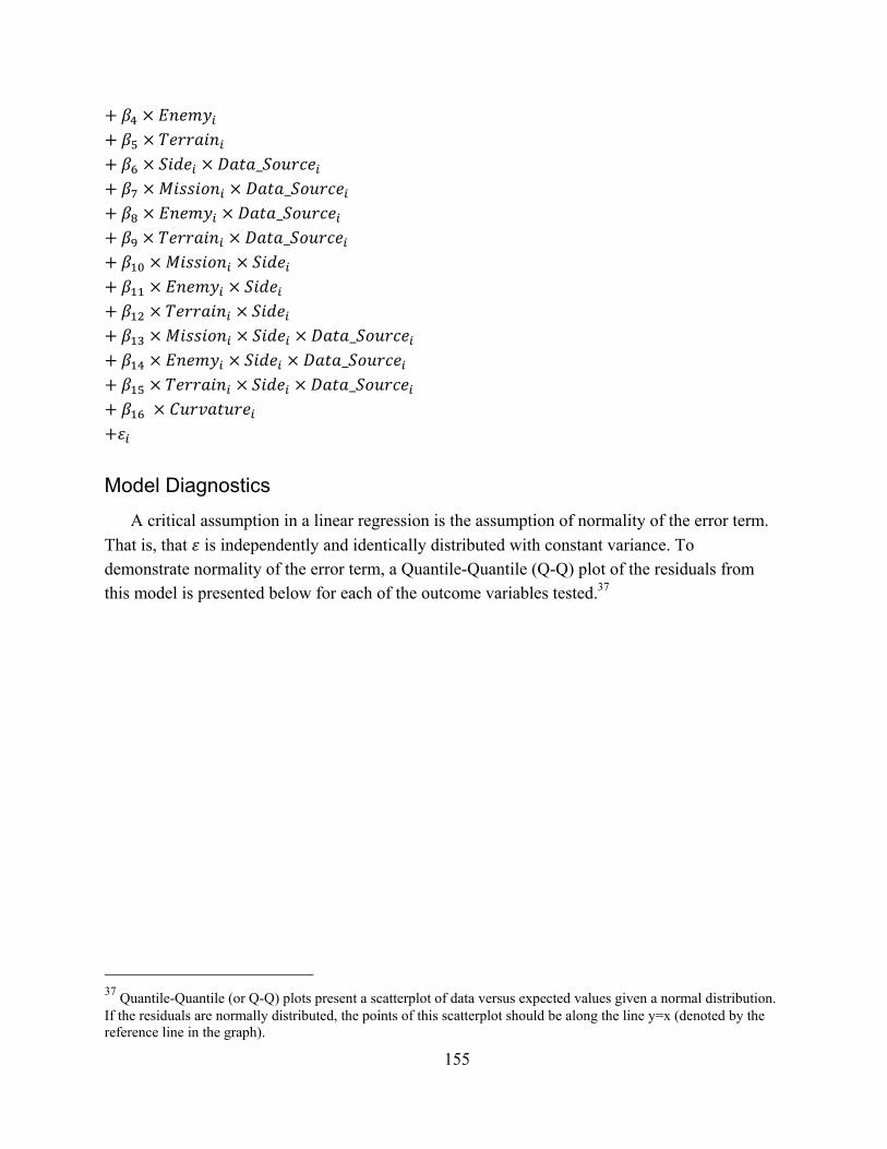
155

_

_

_

_

_

_

_

Model Diagnostics

A critical assumption in a linear regression is the assumption of normality of the error term.

That is, that is independently and identically distributed with constant variance. To demonstrate normality of the error term, a Quantile-Quantile (Q-Q) plot of the residuals from this model is presented below for each of the outcome variables tested.37

37 Quantile-Quantile (or Q-Q) plots present a scatterplot of data versus expected values given a normal distribution. If the residuals are normally distributed, the points of this scatterplot should be along the line y=x (denoted by the reference line in the graph).

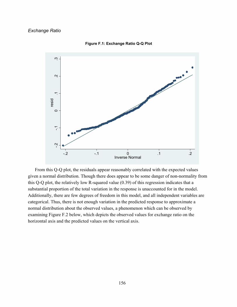
156

Exchange Ratio

Figure F.1: Exchange Ratio Q-Q Plot

From this Q-Q plot, the residuals appear reasonably correlated with the expected values

given a normal distribution. Though there does appear to be some danger of non-normality from this Q-Q plot, the relatively low R-squared value (0.39) of this regression indicates that a substantial proportion of the total variation in the response is unaccounted for in the model. Additionally, there are few degrees of freedom in this model, and all independent variables are categorical. Thus, there is not enough variation in the predicted response to approximate a normal distribution about the observed values, a phenomenon which can be observed by examining Figure F.2 below, which depicts the observed values for exchange ratio on the horizontal axis and the predicted values on the vertical axis.

-.2

-.1

0.1

.2.3

resi

d

-.2 -.1 0 .1 .2Inverse Normal

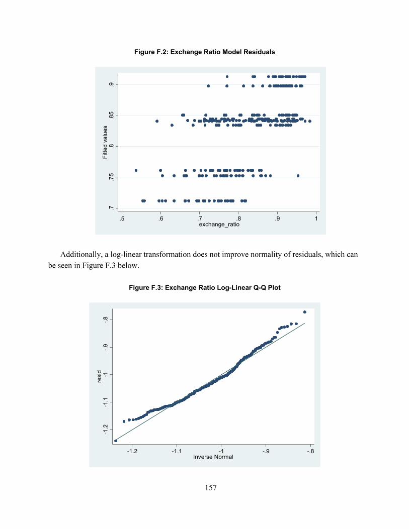
157

Figure F.2: Exchange Ratio Model Residuals

Additionally, a log-linear transformation does not improve normality of residuals, which can

be seen in Figure F.3 below.

Figure F.3: Exchange Ratio Log-Linear Q-Q Plot

.7.7

5.8

.85

.9F

itted

va

lues

.5 .6 .7 .8 .9 1exchange_ratio

-1.2

-1.1

-1-.

9-.

8re

sid

-1.2 -1.1 -1 -.9 -.8Inverse Normal

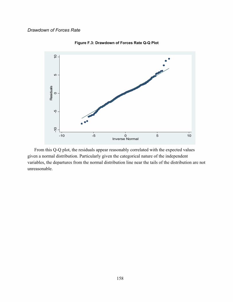
158

Drawdown of Forces Rate

Figure F.3: Drawdown of Forces Rate Q-Q Plot

From this Q-Q plot, the residuals appear reasonably correlated with the expected values

given a normal distribution. Particularly given the categorical nature of the independent variables, the departures from the normal distribution line near the tails of the distribution are not unreasonable.

-10

-50

510

Res

idual

s

-10 -5 0 5 10Inverse Normal

159

Volume of Fire: Rate of Fire

Figure F.4: Rate of Fire Linear Q-Q Plot

From this Q-Q plot, there appears to be a substantial concern of heteroskedasticity. It appears

as though residuals from this model follow a normal distribution save for those at a very low value for rate of fire. Intuitively, these are observations for which the model predicts a negative rate—however, as the rate cannot drop below zero, this is impossible from the data.

To account for this heteroskedasticity, a log-linear transformation was applied to the outcome variable in this regression, the rate of fire. An identical linear regression was run using this log-transformed variable as the outcome, the Q-Q plot for which is located in Figure F.4 below.

-150

-100

-50

050

100

resi

d

-100 -50 0 50 100Inverse Normal

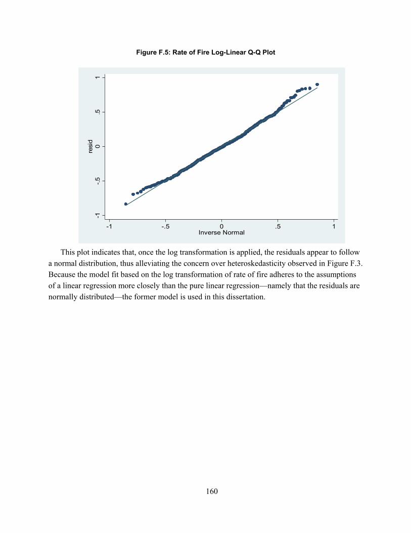
160

Figure F.5: Rate of Fire Log-Linear Q-Q Plot

This plot indicates that, once the log transformation is applied, the residuals appear to follow

a normal distribution, thus alleviating the concern over heteroskedasticity observed in Figure F.3. Because the model fit based on the log transformation of rate of fire adheres to the assumptions of a linear regression more closely than the pure linear regression—namely that the residuals are normally distributed—the former model is used in this dissertation.

-1-.5

0.5

1re

sid

-1 -.5 0 .5 1Inverse Normal

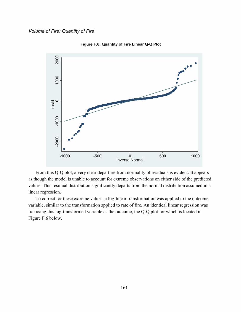
161

Volume of Fire: Quantity of Fire

Figure F.6: Quantity of Fire Linear Q-Q Plot

From this Q-Q plot, a very clear departure from normality of residuals is evident. It appears

as though the model is unable to account for extreme observations on either side of the predicted values. This residual distribution significantly departs from the normal distribution assumed in a linear regression.

To correct for these extreme values, a log-linear transformation was applied to the outcome variable, similar to the transformation applied to rate of fire. An identical linear regression was run using this log-transformed variable as the outcome, the Q-Q plot for which is located in Figure F.6 below.

-20

00-1

000

010

0020

00re

sid

-1000 -500 0 500 1000Inverse Normal

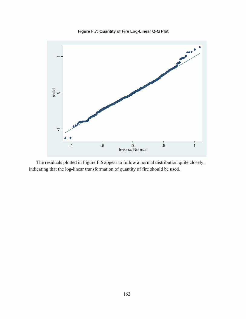
162

Figure F.7: Quantity of Fire Log-Linear Q-Q Plot

The residuals plotted in Figure F.6 appear to follow a normal distribution quite closely,

indicating that the log-linear transformation of quantity of fire should be used.

-10

1re

sid

-1 -.5 0 .5 1Inverse Normal

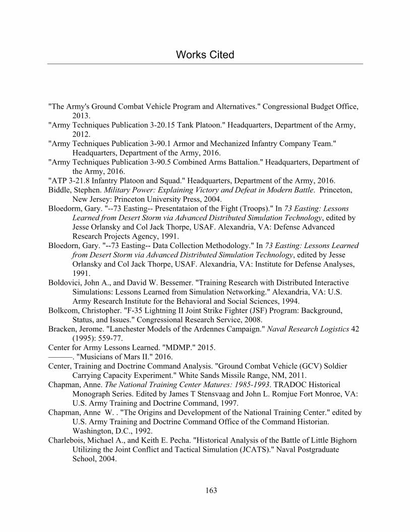
163

Works Cited

"The Army's Ground Combat Vehicle Program and Alternatives." Congressional Budget Office,

2013. "Army Techniques Publication 3-20.15 Tank Platoon." Headquarters, Department of the Army,

2012. "Army Techniques Publication 3-90.1 Armor and Mechanized Infantry Company Team."

Headquarters, Department of the Army, 2016. "Army Techniques Publication 3-90.5 Combined Arms Battalion." Headquarters, Department of

the Army, 2016. "ATP 3-21.8 Infantry Platoon and Squad." Headquarters, Department of the Army, 2016. Biddle, Stephen. Military Power: Explaining Victory and Defeat in Modern Battle. Princeton,

New Jersey: Princeton University Press, 2004. Bloedorm, Gary. "--73 Easting-- Presentataion of the Fight (Troops)." In 73 Easting: Lessons

Learned from Desert Storm via Advanced Distributed Simulation Technology, edited by Jesse Orlansky and Col Jack Thorpe, USAF. Alexandria, VA: Defense Advanced Research Projects Agency, 1991.

Bloedorn, Gary. "--73 Easting-- Data Collection Methodology." In 73 Easting: Lessons Learned from Desert Storm via Advanced Distributed Simulation Technology, edited by Jesse Orlansky and Col Jack Thorpe, USAF. Alexandria, VA: Institute for Defense Analyses, 1991.

Boldovici, John A., and David W. Bessemer. "Training Research with Distributed Interactive Simulations: Lessons Learned from Simulation Networking." Alexandria, VA: U.S. Army Research Institute for the Behavioral and Social Sciences, 1994.

Bolkcom, Christopher. "F-35 Lightning II Joint Strike Fighter (JSF) Program: Background, Status, and Issues." Congressional Research Service, 2008.

Bracken, Jerome. "Lanchester Models of the Ardennes Campaign." Naval Research Logistics 42 (1995): 559-77.

Center for Army Lessons Learned. "MDMP." 2015. ———. "Musicians of Mars II." 2016. Center, Training and Doctrine Command Analysis. "Ground Combat Vehicle (GCV) Soldier

Carrying Capacity Experiment." White Sands Missile Range, NM, 2011. Chapman, Anne. The National Training Center Matures: 1985-1993. TRADOC Historical

Monograph Series. Edited by James T Stensvaag and John L. Romjue Fort Monroe, VA: U.S. Army Training and Doctrine Command, 1997.

Chapman, Anne W. . "The Origins and Development of the National Training Center." edited by U.S. Army Training and Doctrine Command Office of the Command Historian. Washington, D.C., 1992.

Charlebois, Michael A., and Keith E. Pecha. "Historical Analysis of the Battle of Little Bighorn Utilizing the Joint Conflict and Tactical Simulation (JCATS)." Naval Postgraduate School, 2004.

164

Christenson, W.M., Mary Catherine Flythe, Terri J. Walsh, and Robert A. Zirkle. "JCATS Verification and Validation Report." Alexandria, VA: Institute for Defense Analyses, 2002.

Christenson, W.M., and Robert A. Zirkle. "73 Easting Battle Replication--A Janus Combat Simulation." Alexandria, VA: Institute for Defense Analyses, 1992.

"COMBAT XXI." US Army Training and Doctrine Command Analysis Center (TRAC), http://www.trac.army.mil/COMBATXXI.pdf.

Daehner, Endy M. , John Matsumura, Thomas J. Herbert, Jeremy R. Kurz, and Keith Walters. "Integrating Operational Energy Implications into System-Level Combat Effects Modeling: Assessing the Combat Effectiveness and Fuel Use of ABCT 2020 and Current ABCT." Santa Monica, CA: RAND Corporation, 2015.

Davies, Richard W. "A Scientist's First look at the NTC." Pasadena, CA: JPL, 1983. Davison, Anthony Christopher, and David Victor Hinkley. Bootstrap methods and their

application. Vol. 1: Cambridge university press, 1997. "Decisive Action Training Environment at the National Training Center, Volume IV." Center for

Army Lessons Learned, 2016. "Department of Defense Instruction 5000.61 DoD Modeling and Simulation (M&S) Verification,

Validation, and Accreditation (VV&A)." Undersecretary of Defense for Acquisition Technology and Logistics, 2009.

Dryer, David A. "An Analysis of Ground Maneuver Concentration During NTC Deliberate Attack Missions and its Influence on Mission Effectiveness." Masters, Naval Postgraduate School, 1989.

Dupuy, Trevor N. . Numbers, Predictions, and War: Using History to Evaluate Combat Factors and Predict the Outcome of Battles. VA: NOVA Publications, 1985.

Engel, J. H. "A Verification of Lanchester's Law." Journal of the Operations Research Society of America 2, no. 2 (1954): 163-71.

Farr, John V., William R. Johnson, and Robert P. Birmingham. "A Multitiered Approach to Army Acquisition." Defense Acquisition Review Journal 12.2 (2005): 235-45.

Farr, Tom G, Paul A Rosen, Edward Caro, Robert Crippen, Riley Duren, Scott Hensley, Michael Kobrick, et al. "The Shuttle Radar Topography Mission." Reviews of geophysics 45, no. 2 (2007).

"Field Manual 3-90-1 Offense and Defense." Headquarters, Department of the Army, 2013. Fober, Gene W., Jean L. Dyer, and Margaret S. Salter. "Measurement of Performance at the

Joint Readiness Training Center: Tools of Assessment." Research on Measuring and Managing Unit Training Readiness (1994): 39-70.

Fox, Bernard, Michael Boito, John C. Graser, and Obaid Younossi. "Test and Evaluation Trends and Costs for Aircraft and Guided Weapons." Santa Monica, CA: RAND Corporation, 2004.

Fricker, Ronald D. Jr. "Attrition Models of the Ardennes Campaign." Naval Research Logistics (1998).

Gillespie, Thomas C. "Modeling the Combat Power Potential of Marine Corps Close Air Support." Masters, Naval Postgraduate School, 1997.

Glaessgen, E. H. , and D. S. Stargel. "The Digital Twin Paradign for Future NASA and U.S. Air Force Vehicles." Paper presented at the 53rd Structures, Structural Dynamics, and Materials Conference, Honolulu, Hawaii, 2012.

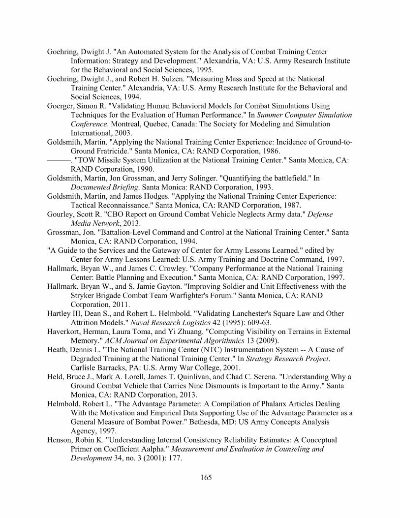
165

Goehring, Dwight J. "An Automated System for the Analysis of Combat Training Center Information: Strategy and Development." Alexandria, VA: U.S. Army Research Institute for the Behavioral and Social Sciences, 1995.

Goehring, Dwight J., and Robert H. Sulzen. "Measuring Mass and Speed at the National Training Center." Alexandria, VA: U.S. Army Research Institute for the Behavioral and Social Sciences, 1994.

Goerger, Simon R. "Validating Human Behavioral Models for Combat Simulations Using Techniques for the Evaluation of Human Performance." In Summer Computer Simulation Conference. Montreal, Quebec, Canada: The Society for Modeling and Simulation International, 2003.

Goldsmith, Martin. "Applying the National Training Center Experience: Incidence of Ground-to-Ground Fratricide." Santa Monica, CA: RAND Corporation, 1986.

———. "TOW Missile System Utilization at the National Training Center." Santa Monica, CA: RAND Corporation, 1990.

Goldsmith, Martin, Jon Grossman, and Jerry Solinger. "Quantifying the battlefield." In Documented Briefing. Santa Monica: RAND Corporation, 1993.

Goldsmith, Martin, and James Hodges. "Applying the National Training Center Experience: Tactical Reconnaissance." Santa Monica, CA: RAND Corporation, 1987.

Gourley, Scott R. "CBO Report on Ground Combat Vehicle Neglects Army data." Defense Media Network, 2013.

Grossman, Jon. "Battalion-Level Command and Control at the National Training Center." Santa Monica, CA: RAND Corporation, 1994.

"A Guide to the Services and the Gateway of Center for Army Lessons Learned." edited by Center for Army Lessons Learned: U.S. Army Training and Doctrine Command, 1997.

Hallmark, Bryan W., and James C. Crowley. "Company Performance at the National Training Center: Battle Planning and Execution." Santa Monica, CA: RAND Corporation, 1997.

Hallmark, Bryan W., and S. Jamie Gayton. "Improving Soldier and Unit Effectiveness with the Stryker Brigade Combat Team Warfighter's Forum." Santa Monica, CA: RAND Corporation, 2011.

Hartley III, Dean S., and Robert L. Helmbold. "Validating Lanchester's Square Law and Other Attrition Models." Naval Research Logistics 42 (1995): 609-63.

Haverkort, Herman, Laura Toma, and Yi Zhuang. "Computing Visibility on Terrains in External Memory." ACM Journal on Experimental Algorithmics 13 (2009).

Heath, Dennis L. "The National Training Center (NTC) Instrumentation System -- A Cause of Degraded Training at the National Training Center." In Strategy Research Project. Carlisle Barracks, PA: U.S. Army War College, 2001.

Held, Bruce J., Mark A. Lorell, James T. Quinlivan, and Chad C. Serena. "Understanding Why a Ground Combat Vehicle that Carries Nine Dismounts is Important to the Army." Santa Monica, CA: RAND Corporation, 2013.

Helmbold, Robert L. "The Advantage Parameter: A Compilation of Phalanx Articles Dealing With the Motivation and Empirical Data Supporting Use of the Advantage Parameter as a General Measure of Bombat Power." Bethesda, MD: US Army Concepts Analysis Agency, 1997.

Henson, Robin K. "Understanding Internal Consistency Reliability Estimates: A Conceptual Primer on Coefficient Aalpha." Measurement and Evaluation in Counseling and Development 34, no. 3 (2001): 177.

166

Hiller, Jack H. "Deriving Useful Lessons From Combat Simulations." In Determinants of Effective Performance: Research on Measuring and Managing Unit Training Readiness, edited by Robert Holz, Jack Hiller and H. McFann, 7-17. Alexandria, VA: U.S. Army Research Institute for the Behavioral and Social Sciences, 1994.

Hoffman, Michael. "Army, Industry Slam CBO's Scathing GCV Report." DoD Buzz, 2013. Holz, Robert, Jack Hiller, and H. McFann, eds. Determinants of Effective Performance:

Research on Measuring and Managing Unit Training Readiness. Alexandria, VA: U.S. Army Research Institute for the Behavioral and Social Sciences, 1994.

Ingber, Lester, Fujio Hirome, and Michael F. Wehner. "Mathematical Comparison of Combat Computer Models to Exercise Data." Mathematical Computer Modeling 15, no. 1 (1991): 65-90.

Jacquet, Carl Rodger, Maj. "A Study of Simulation Effectiveness in Modeling Heavy Combined Arms Combat in Urban Environments." United States Army Command and General Staff College, 2007.

"Joint Conflict and Tactical Simulation (JCATS) Capabilities Brief." Livermore, CA: Lawrence Livermore National Laboratories, 2014.

Kemper, T.R. "Final Technical Report: History of the Combat Training Center Archive." Alexandria, VA: BDM Federal, Inc., 1996.

Kemple, W. G. , and H. J. Larson. "Computer Visualization of Battlefield Tenets." Mathematical Computer Modeling 23, no. 1 (1996): 25-37.

Kerins, James W. , and Nancy K. Atwood. "Concept for a Common Performance Measurement System for Unit Training at the National Training Center (NTC) and with Simulation Networking (SIMNET) Platooon-Defend." BDM Inc., 1990.

Kirin, Stephen J., and Martin Goldsmith. "Mortar Utilization at the Army's Combat Training Centers." Santa Monica, CA: RAND Corporation, 1992.

Kraft, Edward M. "HPCMP CREATE-AV and the Air Force Digital Thread." In 53rd AIAA Aerospace Sciences Meeting. Kissimmee, Florida: AIAA SciTech, 2015.

Lambert, Garrett R., Morris Hayes, LTC Christopher P. Holmes, David Hull, LTC Shawn Lucas, Rick Pierce, Martha Roper, Thomas Stadterman, and Saul Solis. "Ground Combat Vehicle (GCV) Analysis of Alternatives (AoA) Final Report." White Sands Missile Range, NM: TRADOC Analysis Center, 2011.

Lamont, Robert W. "Direct Fire Synchronization." Masters, Naval Postgraduate School, 1992. Lanchester, Frederick William. Aircraft in Warfare: The Dawn of the Fourth Arm. Constable

Limited, 1916. Larson, H. J., W. G. Kemple, and D. A. Dryer. "Graphical Displays of Synchronization of

Tactical Units." Mathematical Computer Modeling 23, no. 1 (1996): 15-24. Levine, Robert A., James S. Hodges, and Martin Goldsmith. "Utilizing the Data from the Army's

National Training Center: Analytical Plan." In RAND Note. Santa Monica, CA: RAND Corporation, 1986.

Li, Chenzhao, Sankaran Mahadevan, You Ling, Sergio Choze, and Liping Wang. "Dynamic Bayesian Network for Aircraft Wing Health Monitoring Digital Twin." AIAA Journal 0, no. 0 (2017).

Lopuhaa, Hendrik P, and Peter J Rousseeuw. "Breakdown Points of Affine Equivariant Estimators of Multivariate Location and Covariance Matrices." The Annals of Statistics (1991): 229-48.

167

Lucas, Thomas W., and John A Dinges. "The Effect of Battle Circumstances on Fitting Lanchester Equations to the Battle of Kursk." Military Operations Research (2004).

Lucas, Thomas W., and Turker Turkes. "Fitting Lanchester Equations to the Battles of Kursk and Ardennes." Naval Research Logistics 51 (2004).

"M1A1 Abrams." Military Today, http://www.military-today.com/tanks/m1a1_abrams.htm. Marshall, S.L.A. Men Against Fire: The Problem of Battle Command in Future War. New York:

William Morrow & Co., 1947. Matsumura, John, Randall Steeb, John Gordon IV, Thomas J. Hervert, Russel W. Glenn, and

Paul S. Steinberg. "Lightning Over Water: Sharpening America's Light Forces for Rapid Reaction Missions." Santa Monica, CA: RAND Corporation, 2000.

Nelson, Michael S. "Graphical Methods for Depicting Combat Units." Masters, Naval Postgraduate School, 1992.

North, Bernard V, David Curtis, and Pak C Sham. "A note on the calculation of empirical P values from Monte Carlo procedures." The American Journal of Human Genetics 71, no. 2 (2002): 439-41.

"NTC SCORPIONS' SAWE/MILES II (Simulated Area Weapons Effects/Multiple-Integrated Laser Engagement System II), Handbook No. 98-1." Ft. Irwin, CA: National Training Center Operations Group, 1998.

O'Mara, Francis E. "Relationship of Training and Personnel Factors to Combat Performance." Monterey, CA: U.S. Army Research Institute for the Social and Behavioral Sciences, 1989.

Parker, Joel R. "Methodology and Analysis of Ground Maneuver Synchronization at the National Training Center." Masters, Naval Postgraduate School, 1990.

Peterson, Jeffrey D. "The Effect of Personnel Stability on Organizational Performance: Do Battalions with Stable Command Groups Achieve Higher Training Proficiency at the National Training Center?", Pardee RAND Graduate School, 2008.

Pickering, William H., Charles H. Terhune, Jr., Richard A. Montgomery, Lawrence Caldwell, David Kassing, Christopher Layne, Leslie Lewis, et al. "Arroyo Center Report Collection." Pasadena, CA: Caltech JPL, 1985.

Plackett, R. L. , and J.P. Burman. "The Design of Optimum Multifactorial Experiments." Biometrika 33, no. 4 (1946): 305-25.

"RADGUNS: Radar-Directed Gun System Simulation." Defense Systems Information Analysis Center, https://www.dsiac.org/resources/models_and_tools/radguns.

"Recomended Practices Guide: Data Verification and Validation (V&V) for Legacy Simulations." edited by Modeling and Simulation Coordination Office, 2006.

Rothenberg, Jeff, Walter Stanley, George Hanna, and Mark Ralston. "Data Verification, Validation, and Certification (VV&C): Guidelines for Modeling and Simulation." Santa Monica, CA: RAND Corporation, 1997.

Rotte, Ralph, and Christoph Schmidt. "On the Production of Victory; Emperical Determinants of Battlefield Success in Modern War." Defesnse and Peace Economics 14, no. 3 (2003): 175-92.

Saltelli, Andrea. "Making Best Use of Model Evaluations to Compute Sensitivity Indices." Computer Physics Communications 145, no. 2 (2002): 280-97.

Saltelli, Andrea, Marco Ratto, Terry Andres, Francesca Campolongo, Jessica Cariboni, Debora Gatelli, Michaela Saisana, and Stefano Tarantola. Global Sensitivity Analysis: the Primer. John Wiley & Sons, 2008.

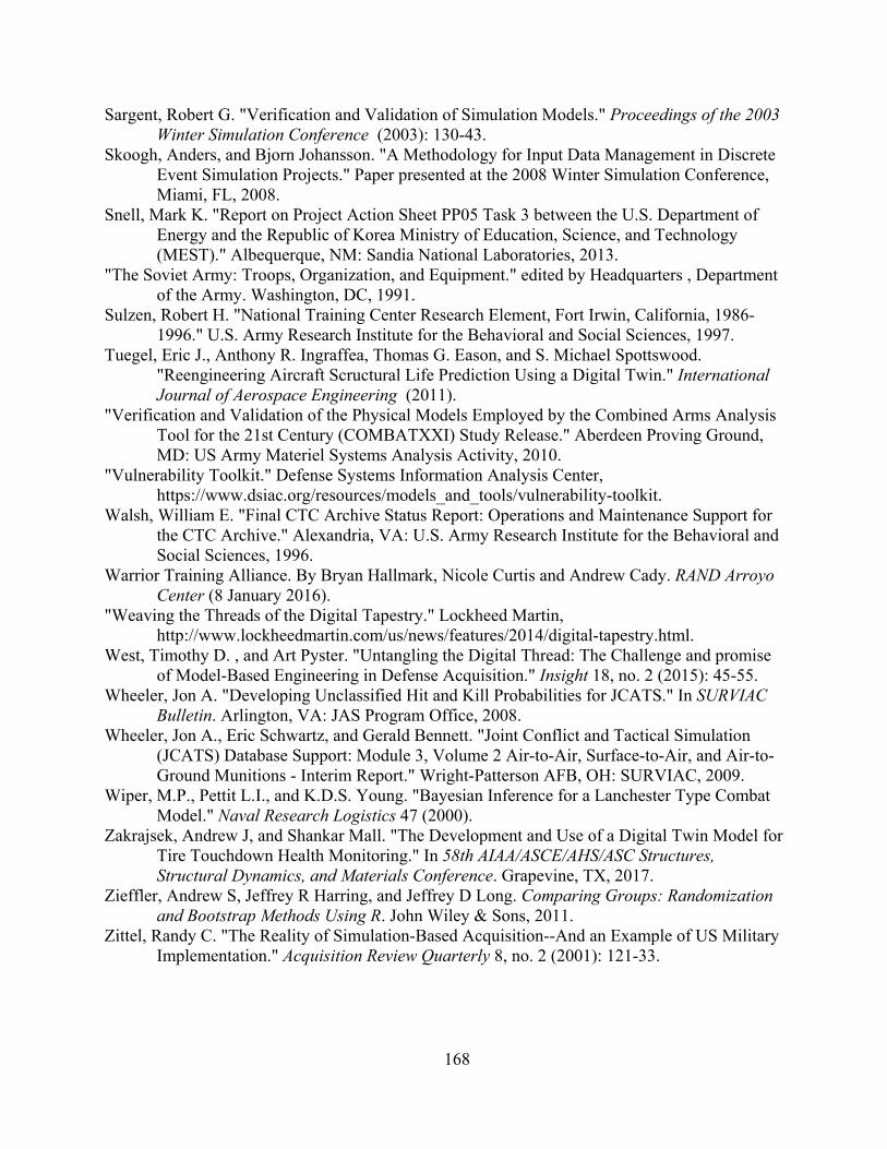
168

Sargent, Robert G. "Verification and Validation of Simulation Models." Proceedings of the 2003 Winter Simulation Conference (2003): 130-43.

Skoogh, Anders, and Bjorn Johansson. "A Methodology for Input Data Management in Discrete Event Simulation Projects." Paper presented at the 2008 Winter Simulation Conference, Miami, FL, 2008.

Snell, Mark K. "Report on Project Action Sheet PP05 Task 3 between the U.S. Department of Energy and the Republic of Korea Ministry of Education, Science, and Technology (MEST)." Albequerque, NM: Sandia National Laboratories, 2013.

"The Soviet Army: Troops, Organization, and Equipment." edited by Headquarters , Department of the Army. Washington, DC, 1991.

Sulzen, Robert H. "National Training Center Research Element, Fort Irwin, California, 1986-1996." U.S. Army Research Institute for the Behavioral and Social Sciences, 1997.

Tuegel, Eric J., Anthony R. Ingraffea, Thomas G. Eason, and S. Michael Spottswood. "Reengineering Aircraft Scructural Life Prediction Using a Digital Twin." International Journal of Aerospace Engineering (2011).

"Verification and Validation of the Physical Models Employed by the Combined Arms Analysis Tool for the 21st Century (COMBATXXI) Study Release." Aberdeen Proving Ground, MD: US Army Materiel Systems Analysis Activity, 2010.

"Vulnerability Toolkit." Defense Systems Information Analysis Center, https://www.dsiac.org/resources/models_and_tools/vulnerability-toolkit.

Walsh, William E. "Final CTC Archive Status Report: Operations and Maintenance Support for the CTC Archive." Alexandria, VA: U.S. Army Research Institute for the Behavioral and Social Sciences, 1996.

Warrior Training Alliance. By Bryan Hallmark, Nicole Curtis and Andrew Cady. RAND Arroyo Center (8 January 2016).

"Weaving the Threads of the Digital Tapestry." Lockheed Martin, http://www.lockheedmartin.com/us/news/features/2014/digital-tapestry.html.

West, Timothy D. , and Art Pyster. "Untangling the Digital Thread: The Challenge and promise of Model-Based Engineering in Defense Acquisition." Insight 18, no. 2 (2015): 45-55.

Wheeler, Jon A. "Developing Unclassified Hit and Kill Probabilities for JCATS." In SURVIAC Bulletin. Arlington, VA: JAS Program Office, 2008.

Wheeler, Jon A., Eric Schwartz, and Gerald Bennett. "Joint Conflict and Tactical Simulation (JCATS) Database Support: Module 3, Volume 2 Air-to-Air, Surface-to-Air, and Air-to-Ground Munitions - Interim Report." Wright-Patterson AFB, OH: SURVIAC, 2009.

Wiper, M.P., Pettit L.I., and K.D.S. Young. "Bayesian Inference for a Lanchester Type Combat Model." Naval Research Logistics 47 (2000).

Zakrajsek, Andrew J, and Shankar Mall. "The Development and Use of a Digital Twin Model for Tire Touchdown Health Monitoring." In 58th AIAA/ASCE/AHS/ASC Structures, Structural Dynamics, and Materials Conference. Grapevine, TX, 2017.

Zieffler, Andrew S, Jeffrey R Harring, and Jeffrey D Long. Comparing Groups: Randomization and Bootstrap Methods Using R. John Wiley & Sons, 2011.

Zittel, Randy C. "The Reality of Simulation-Based Acquisition--And an Example of US Military Implementation." Acquisition Review Quarterly 8, no. 2 (2001): 121-33.