Use of a Radar Wind Profiler and Sodar to Characterize PM 2.5 Air Pollution in Cleveland, Ohio Clinton P. MacDonald 1, Adam N. Pasch 1, Robert Gilliam.

Use of a Radar Wind Profiler and Sodar to Characterize PM2.5 Air Pollution in Cleveland, Ohio

Clinton P. MacDonald1, Adam N. Pasch1, Robert Gilliam2, Charley A. Knoderer1, Paul T. Roberts1, and Gary Norris2

1Sonoma Technology, Inc.2U.S. Environmental Protection Agency

Presented at the National Air Quality ConferencesMarch 7-10, 2011

San Diego, CA

4070

2

About Cleveland

• Geography

• Population~430,000 Cleveland

• Emissions– Large power plants,

steel mills, marine vessels, and on-road vehicles

• Non-attainment for PM2.5

Regional scale

Cleveland

3

About EPA’s CMAPS

• Cleveland Multiple Air Pollutant Study from August 2009 to August 2010– identify particulate matter (PM) and mercury (Hg) sources

– characterize emissions

– understand the role of meteorology

– characterize the spatial and temporal variability of multi-pollutant exposures

• Two five-week intensives

• EPA Principal Investigators include Gary Norris, Matthew Landis, and Ian Gilmour

4

Complex PM2.5 Concentrations

Urban PM2.5

Upwind PM2.5

Hourly PM2.5 Concentrations

5

10

15

20

25

30

35

40

45

50

55

0 2 4 6 8 10 12 14 16 18 20 22

Hour (EST)

Co

nc

en

tra

tio

n (

ug

/m3

)

BARR

MEDINA

ST_THEODOS

5

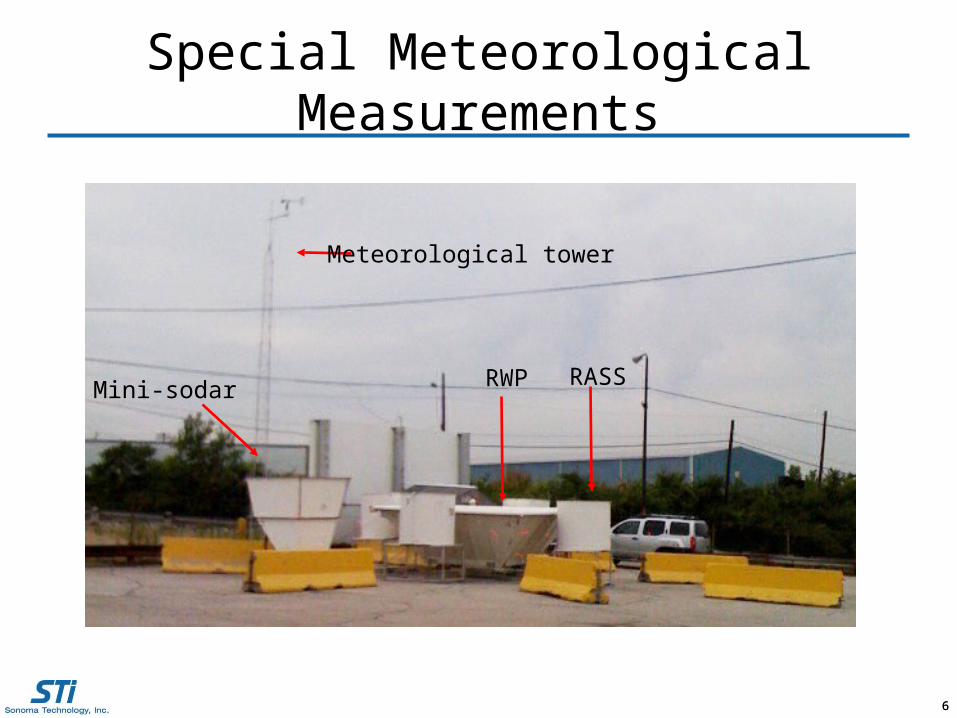
Understand the Role of Meteorology

• Radar wind profiler (RWP)

• Radio acoustic sounding system (RASS)

• Mini-sodar

• Surface meteorology

6

Special Meteorological Measurements

6

Meteorological tower

Mini-sodar RWP RASS

7

Methods

• Case Studies

• Episodes* versus non-episodes:

– Diurnal PM2.5

– Large-scale meteorology

– Mixing height

– Boundary layer winds

• RWP, RASS, and mini-sodar

• WRF 4-km backward trajectories (EPA)

• Hybrid Single-Particle Lagrangian Integrated Trajectory (HYSPLIT) backward trajectories

• Representativeness of CMAPS

7

*24-hr PM2.5 concentrations > 34.4 μg/m3 at St. Theodosis or G.T. Craig

Episode Date

Maximum 24-hr Average PM2.5

Concentration (μg/m3)

8/9/2009 37

8/15/2009 54

8/16/2009 51

2/2/2010 41

2/3/2010 45

2/20/2010 39

2/21/2010 38

3/8/2010 42

3/9/2010 62

3/10/2010 39

3/11/2010 42

8

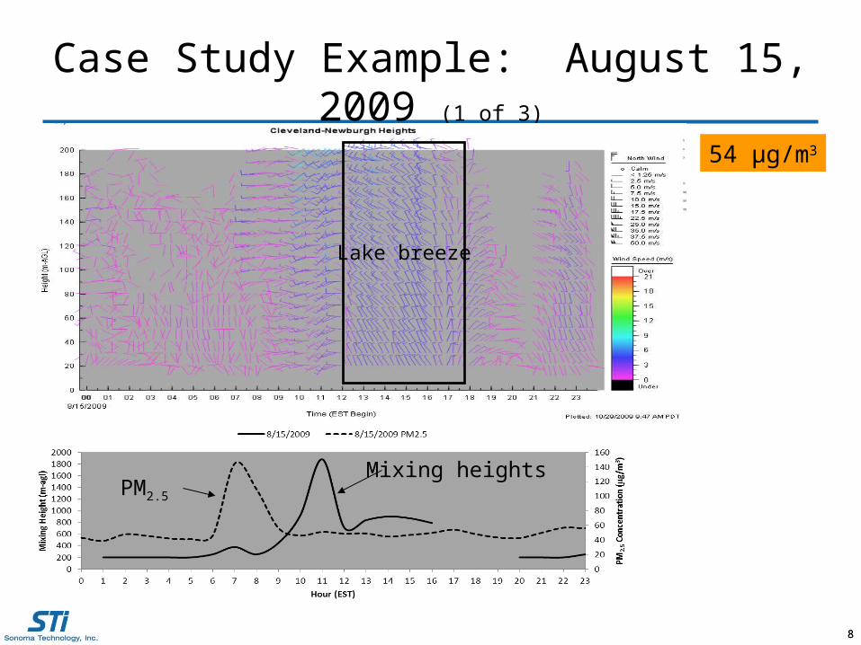
Case Study Example: August 15, 2009 (1 of 3)

8

54 μg/m3

Lake breeze

Mixing heightsPM2.5

9

Case Study Example: August 15, 2009 (2 of 3)

9

54 μg/m3

Southerly winds aloft

Mixing height Lake boundary layer

CB

L

10

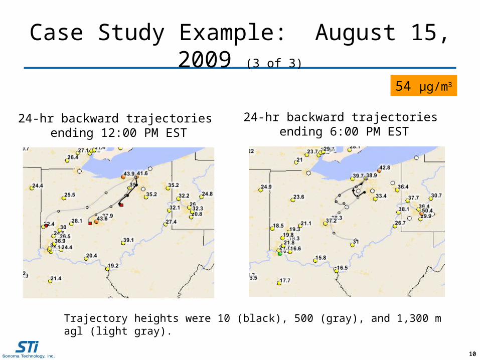
Case Study Example: August 15, 2009 (3 of 3)

10

24-hr backward trajectories ending 12:00 PM EST

Trajectory heights were 10 (black), 500 (gray), and 1,300 m agl (light gray).

54 μg/m3

24-hr backward trajectories ending 6:00 PM EST

11

Case Study Example: March 08, 2010

High ventilation driven by moderate winds, but recirculation. 42 μg/m3

12

Results: Episode vs. Non-episode: PM2.5

12

13

Results: Episode vs. Non-episode: Peak Mixing

Summer

Winter

Episode

Non-Episode

14

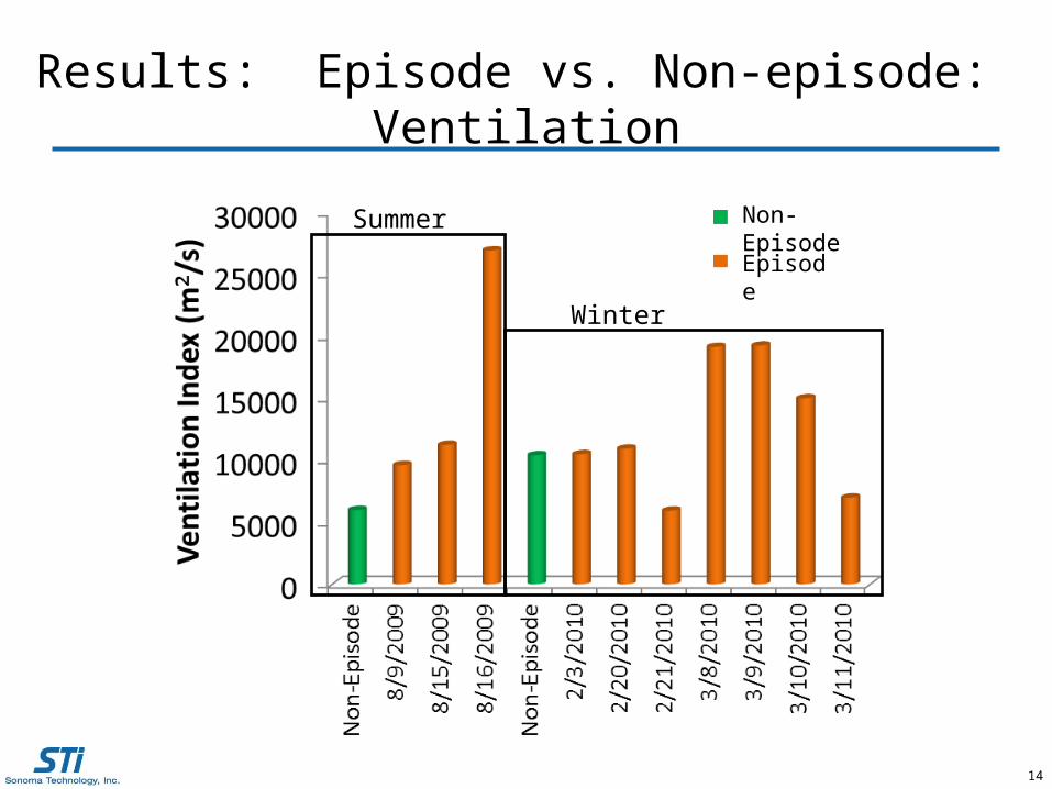
Results: Episode vs. Non-episode: Ventilation

Summer

Winter

Episode

Non-Episode

15

Results: Episode vs. Non-episode: Transport

Episode DateRWP/Sodar

NAM WRF ConcensusLocal Carryover of

Upwind AQI

8/9/2009 M S S/M Mod

8/15/2009 S S M S Mod

8/16/2009 M M M M Mod

2/2/2010 M S S S Mod

2/3/2010 M M S M Mod

2/20/2010 M M M M Good/Mod

2/21/2010 S S S S Mod

3/8/2010 M M M Good/Mod

3/9/2010 M S S/M Mod

3/10/2010 L L L Mod/USG

3/11/2010 L M M/L Mod

S = 24-hr transport < ~100 kmM = 24-hr transport between ~100 and 350 kmL = 24-hr transport > ~400 km

16

Summary of Episodes (1 of 2)

• Moderate AQI carryover or transport on all days

• Summer episodes (3): high ventilation – High mixing heights and moderate boundary layer

winds from the southwest (2)– High mixing heights, but light winds with a lake breeze

(1)

16

17

Summary of Episodes (2 of 2)

Winter episodes (7): wide variety of conditions– High ventilation driven by moderate winds, but

recirculation (3)– Moderate ventilation driven by moderate west

winds (2)– Low ventilation (low mixing and light winds) (2)

17