JSS Journal of Statistical Software November 2010, Volume 37, Issue 6. http://www.jstatsoft.org/ US Census Spatial and Demographic Data in R: The UScensus2000 Suite of Packages Zack W. Almquist University of California, Irvine Abstract The US Decennial Census is arguably the most important data set for social science research in the United States. The UScensus2000 suite of packages allows for convenient handling of the 2000 US Census spatial and demographic data. The goal of this article is to showcase the UScensus2000 suite of packages for R, to describe the data contained within these packages, and to demonstrate the helper functions provided for handling this data. The UScensus2000 suite is comprised of spatial and demographic data for the 50 states and Washington DC at four different geographic levels (block, block group, tract, and census designated place). The UScensus2000 suite also contains a number of functions for selecting and aggregating specific geographies or demographic information such as metropolitan statistical areas, counties, etc. These packages rely heavily on the spatial tools developed by Bivand, Pebesma, and G´ omez-Rubio (2008), i.e., the sp and maptools packages. This article will provide the necessary background for working with this data set, helper functions, and finish with an applied spatial statistics example. Keywords : spatial data, spatial analysis, spatial data handling, US Census, demography, R. 1. Introduction The US Decennial Census is arguably the most important data set for social science research in the United States. The US conducts a census of the entire population every ten years to de- termine proper Congressional representation based on the population. Along with population counts, the US Census Bureau collects thousands of basic demographic characteristics and aggregates these into various geographical regions (represented as polygons). This paper will provide an overview of the UScensus2000 suite of packages. The packages contain geographic representations of the 2000 US Census, a common set of demographic variables, and various helper functions. These packages also provide easy access to the US Census data for R users, including: Improved accessibility, polygon/spatial data management, detailed meta-data and

Welcome message from author
This document is posted to help you gain knowledge. Please leave a comment to let me know what you think about it! Share it to your friends and learn new things together.
Transcript
JSS Journal of Statistical SoftwareNovember 2010, Volume 37, Issue 6. http://www.jstatsoft.org/
US Census Spatial and Demographic Data in R:
The UScensus2000 Suite of Packages
Zack W. AlmquistUniversity of California, Irvine
Abstract
The US Decennial Census is arguably the most important data set for social scienceresearch in the United States. The UScensus2000 suite of packages allows for convenienthandling of the 2000 US Census spatial and demographic data. The goal of this articleis to showcase the UScensus2000 suite of packages for R, to describe the data containedwithin these packages, and to demonstrate the helper functions provided for handlingthis data. The UScensus2000 suite is comprised of spatial and demographic data forthe 50 states and Washington DC at four different geographic levels (block, block group,tract, and census designated place). The UScensus2000 suite also contains a number offunctions for selecting and aggregating specific geographies or demographic informationsuch as metropolitan statistical areas, counties, etc. These packages rely heavily on thespatial tools developed by Bivand, Pebesma, and Gomez-Rubio (2008), i.e., the sp andmaptools packages. This article will provide the necessary background for working withthis data set, helper functions, and finish with an applied spatial statistics example.
Keywords: spatial data, spatial analysis, spatial data handling, US Census, demography, R.
1. Introduction
The US Decennial Census is arguably the most important data set for social science researchin the United States. The US conducts a census of the entire population every ten years to de-termine proper Congressional representation based on the population. Along with populationcounts, the US Census Bureau collects thousands of basic demographic characteristics andaggregates these into various geographical regions (represented as polygons). This paper willprovide an overview of the UScensus2000 suite of packages. The packages contain geographicrepresentations of the 2000 US Census, a common set of demographic variables, and varioushelper functions. These packages also provide easy access to the US Census data for R users,including: Improved accessibility, polygon/spatial data management, detailed meta-data and
2 UScensus2000: US Census Spatial and Demographic Data in R
conveniently sourced inbuilt documentation.
The UScensus2000 suite of packages integrates seamlessly with the geographical informationsystem Bivand et al. (2008) built for the R programing language (R Development Core Team2010). In their book GIS: A Computing Perspective, Worboys and Duckham (2004) explainthat “[a] geographic information system (GIS) is a special type of computer-based informationsystem tailored to store, process, and manipulate geospatial data.”This type of geospatial datahas proven to be extremely valuable to a diverse range of fields, from geology to economics;any scientist who wishes to display and analyze spatial data. Worboys and Duckham (2004)proceeds to write “[a]t the heart of any GIS is the database, which organizes data in a formthat is easy to store and retrieve.” That is to say, managing spatial data is a difficult taskdue to the large amount of mathematically complex polygon files and accompanying covariateinformation. Consequently, a competently built data management system for handling largescale geospatial data is an important enterprise, crucial to enabling the analyst to performhis or her task at optimal efficiency.
These packages represent a template for the managing of spatial and demographic cen-sus data, which might be used for other US Censuses, and similar types of data world-wide (e.g., http://2010.census.gov/2010census/, https://international.ipums.org,http://epp.eurostat.ec.europa.eu/, etc.). Specifically, we take advantage of the rigidCensus hierarchy of geographic scale and data attributes (e.g., administrative borders) tosimplify common tasks in spatial analysis, such as data acquisition, plotting, map overlayfunctions, and statistical analysis. The US Census geography maintains a strict hierarchysuch that states contain counties, counties contain tracts, tracts contain block groups, andblock groups contain blocks. Strictly speaking there should be no overlap between each con-tainer level. The US Census data files are publicly available, but are maintained in a seriesof disparate flat text files which include the actual demographic information, shapefiles, andrelevant accompanying documentation (explaining the organization of the files, definitions ofvariables, etc.). The UScensus2000 suite provides an intuitive organization of these separateentities into a single coherent package that includes inbuilt documentation, help files, exam-ples, and a series of general helper functions for identifying and extracting important anduseful subsets of the spatial and demographic data. These helper functions allow the user toextract and aggregate geographies, demographic characteristics, and also allow the user toadd demographic data from the US Census Summary File 100 (SF1) percent files (US CensusBureau 2001).
The US Census Bureau aggregates data at four basic geographic levels: county, tract, blockgroup, and block. In addition, two other geographic conglomerations, metropolitan statisticalareas (MSA) and census designated places (CDP), are defined. The first four geographic areas(county, tract, block group, and block) exist in a hierarchical system (US Census Bureau 2001,Figure 1). This is explained in great detail at either the US Census website (http://www.census.gov/) or the SF1 technical report (US Census Bureau 2001). MSAs are composedof counties, and census designated places are political entities defined by states and the USCensus Bureau, e.g., incorporated and unincorporated cities, townships, etc. (US CensusBureau 2001).
The US Census Bureau provides polygon representations of the geographic data in a formatknown as shapefiles (or ESRI shapefiles) through the TIGER/LINE data repository (http://www.census.gov/geo/www/tiger/) and provides access to demographic data through the USCensus Bureau’s online data extractor, American FactFinder (http://factfinder.census.
Journal of Statistical Software 3
Figure 1: Representation of block, block group, tract, and county hierarchy in US Censusgeography. Note that CDPs do not observe boundaries of the other polygons and that MSAsare composed of counties.
gov/). The shapefiles are meant for use in geographic information systems (GIS) software –such as GRASS and ArcGIS.
A myriad of reasons exist to want such data readily available in an R based format, includingsimulation modeling, spatial statistics, GIS-style plotting and so forth; however, this data hasnot been imported into R on a large scale due to the complexity and size of the data set.Fortunately, a number of the basic tools necessary for this task have been implemented in Rincluding the maptools and sp packages (Lewin-Koh and Bivand 2009; Pebesma and Bivand2005). This article will concentrate on covering the relevant information needed to manipulatethe 2000 US Census geographic and demographic data contained within the UScensus2000suite. This article will introduce functions for acquiring specific conglomerations of censusdata: Counties, MSA, and cities (county, MSA and poly.clipper), as well as selecting de-mographics (demographics); and functions for adding data to these packages’ spatial objects(demographics.add). In addition to addressing examples of these functions and some stan-dard uses of these functions, a spatial statistics application using the spdp package (Bivand2009) is demonstrated.
2. Data structure basics
The UScensus2000 suite is composed of six packages – four of which contain spatial anddemographic data – each of which maintains the same basic nomenclature and data struc-
4 UScensus2000: US Census Spatial and Demographic Data in R
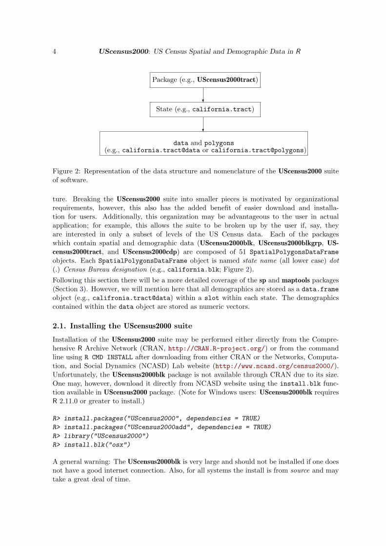
Package (e.g., UScensus2000tract)
State (e.g., california.tract)
data and polygons(e.g., california.tract@data or california.tract@polygons)
?
?
Figure 2: Representation of the data structure and nomenclature of the UScensus2000 suiteof software.
ture. Breaking the UScensus2000 suite into smaller pieces is motivated by organizationalrequirements, however, this also has the added benefit of easier download and installa-tion for users. Additionally, this organization may be advantageous to the user in actualapplication; for example, this allows the suite to be broken up by the user if, say, theyare interested in only a subset of levels of the US Census data. Each of the packageswhich contain spatial and demographic data (UScensus2000blk, UScensus2000blkgrp, US-census2000tract, and UScensus2000cdp) are composed of 51 SpatialPolygonsDataFrame
objects. Each SpatialPolygonsDataFrame object is named state name (all lower case) dot(.) Census Bureau designation (e.g., california.blk; Figure 2).
Following this section there will be a more detailed coverage of the sp and maptools packages(Section 3). However, we will mention here that all demographics are stored as a data.frame
object (e.g., califronia.tract@data) within a slot within each state. The demographicscontained within the data object are stored as numeric vectors.
2.1. Installing the UScensus2000 suite
Installation of the UScensus2000 suite may be performed either directly from the Compre-hensive R Archive Network (CRAN, http://CRAN.R-project.org/) or from the commandline using R CMD INSTALL after downloading from either CRAN or the Networks, Computa-tion, and Social Dynamics (NCASD) Lab website (http://www.ncasd.org/census2000/).Unfortunately, the UScensus2000blk package is not available through CRAN due to its size.One may, however, download it directly from NCASD website using the install.blk func-tion available in UScensus2000 package. (Note for Windows users: UScensus2000blk requiresR 2.11.0 or greater to install.)
R> install.packages("UScensus2000", dependencies = TRUE)
R> install.packages("UScensus2000add", dependencies = TRUE)
R> library("UScensus2000")
R> install.blk("osx")
A general warning: The UScensus2000blk is very large and should not be installed if one doesnot have a good internet connection. Also, for all systems the install is from source and maytake a great deal of time.
Journal of Statistical Software 5
3. The sp and maptools packages
The sp (Pebesma and Bivand 2005) and maptools (Lewin-Koh and Bivand 2009) packagesprovide the backbone of the UScensus2000 suite of packages; to be fully conversant in spatialanalysis and spatial data in R one should read Bivand et al. (2008)’s book Applied SpatialData Analysis with R. All spatial data stored in the UScensus2000 suite are of the formSpatialPolygonsDataFrame (e.g., california.tract is a SpatialPolygonsDataFrame ob-ject). SpatialPolygonsDataFrame objects are a so-called S4 class object in R and con-tain detailed attribute data. In general, each SpatialPolygonsDataFrame object may betreated like a data.frame object – which means the standard data.frame methods apply,e.g., oregon.tract$pop2000) – which is characterized by special attributes for spatial infor-mation. The two most important of these attributes are the bounding box and the coordinatereference system (CRS). The bounding box, which is used mostly for plotting, represents theminimum and maximum values of the spatial polygons. The CRS represents the projectionof the data (commonly this is Longitude and Latitude). The sp and maptools packages alsoprovide a number of routines so that R knows how to perform many common tasks such asplot and summary.
There are two basic methods for directly accessing polygon and demographic data inSpatialPolygonsDataFrame objects. The first is the slot method (accessed by either slot()or @-symbol). The second is through the standard method calls: [,], [[ ]] and $. Take forexample the SpatialPolygonsDataFrame object oregon.tract:
R> library("UScensus2000tract")
R> data("oregon.tract")
R> slotNames(oregon.tract)
[1] "data" "polygons" "plotOrder" "bbox" "proj4string"
The function slotNames provides us the names of the five objects which comprise eachSpatialPolygonsDataFrame. Excerpts describing each of these objects, pulled from theirrespective help files (Pebesma and Bivand 2005; Lewin-Koh and Bivand 2009), are shownbelow:
data: Object of class data.frame; the number of rows in data should equal the number ofPolygons class objects (help("SpatialPolygonsDataFrame")).
polygons: Sets of spatial coordinates to create spatial data, or retrieve spatial coordinates(help("polygons")).
plotOrder: Object of class integer; integer array giving the order in which objects shouldbe plotted (help("SpatialPolygons-class")).
bbox: Retrieves spatial bounding box from spatial data (help("bbox")).
proj4string: Sets or retrieves projection attributes on classes extending spatial data(help("proj4string")).
Each of the four data packages of the UScensus2000 suite is broken down into
6 UScensus2000: US Census Spatial and Demographic Data in R
51 SpatialPolygonsDataFrame objects which are comprised, in part, of polygon and de-mographic data (see the example above). One may directly access the list of polygondata through the slot(*, "polygons") and the data.frame object of demographic datavia slot(*, "data"). There are two types of information stored within the "data" slot
of each SpatialPolygonsDataFrame objects in the UScensus2000 suite: ID variables, whichare stored as factors, and demographic variables, which are stored as numeric. All SF1data is count data and represents X number of the given variable at a given geography (e.g.,california.tract$white provides all counts of white individuals in each tract in Califor-nia, and california.tract$hh.units provides all counts of household units in each tract inCalifornia).
Some useful functions provided in the sp package include summary, bbox, proj4string,plot/spplot, spRbind, unionSpatialPolygons and overlay. The summary function pro-vides a standard summary of the sp objects; proj4string provides for some manipula-tion of the CRS; the bbox function pulls out the bounding box of the entire object (e.g.,bbox(california.tract)), where a bounding box is a rectangle of minimum and maximumcoordinates of the sp object. spRbind allows for combining two sp objects of the same typewith the same data.frame columns, and unionSpatialPolygons allows one to combine sp
polygons into larger polygons. These functions are useful for summarizing, plotting and/orstatistical techniques. The overlay function is a particularly useful command and performsa type of point-in-polygon procedure (i.e. overlay(points, polygons)).
It is always good practice to run a summary on the data; however, users should be awarethat running summary directly on a SpatialPolygonsDataFrame results in both the sum-mary for data.frame information and the SpatialPolygons information. To generate theSpatialPolygons summary information, one applies the following code:
R> summary(as(oregon.tract, "SpatialPolygons"))
Object of class SpatialPolygons
Coordinates:
min max
r1 -124.55244 -116.4635
r2 41.99179 46.2710
Is projected: FALSE
proj4string :
[+proj=longlat +datum=NAD83 +ellps=GRS80 +towgs84=0,0,0]
If one wants the bounding box information or the CRS information one may do the following:
R> bbox(oregon.tract)
min max
r1 -124.55244 -116.4635
r2 41.99179 46.2710
R> proj4string(oregon.tract)
[1] " +proj=longlat +datum=NAD83 +ellps=GRS80 +towgs84=0,0,0"
Journal of Statistical Software 7
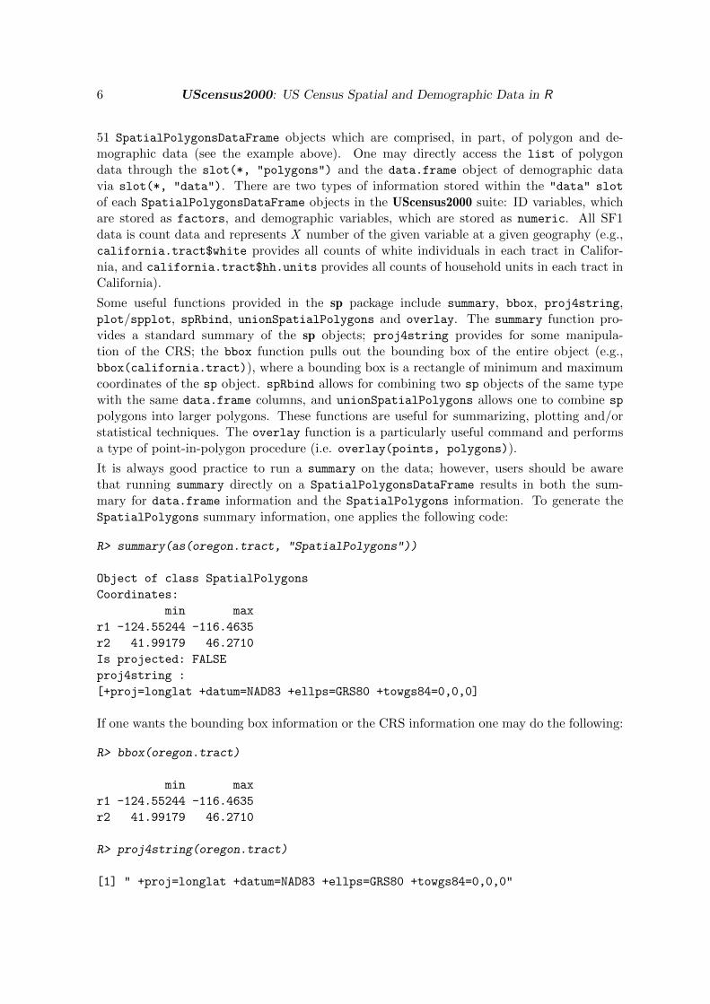
Figure 3: A plot of the Pacific Northwest.
Combining data is another common activity and is made straight forward through the sp
package. There are two basic types of data integration: spRbind – for binding spatial dataand unionSpatialPolygons – for aggregating spatial data.
Take for example the case of the Pacific Northwest (Oregon, Washington, and Idaho; Figure 3).A user might want to have a single data object which contains all the spatial and demographicdata of the Pacific Northwest, or one might want to simply have the border of the PacificNorthwest. The following example provides the necessary code:
R> data("washington.tract")
R> data("idaho.tract")
R> pacificNW <- spRbind(oregon.tract, washington.tract)
R> pacificNW <- spRbind(pacificNW, idaho.tract)
R> summary(as(pacificNW, "SpatialPolygons"))
Object of class SpatialPolygons
Coordinates:
min max
x -124.73317 -111.04356
y 41.98806 49.00249
Is projected: FALSE
proj4string :
[+proj=longlat +datum=NAD83 +ellps=GRS80 +towgs84=0,0,0]
R> gpclibPermit()
R> pacNWol <- unionSpatialPolygons(pacificNW,
+ rep("x", length(slot(pacificNW, "polygons"))))
R> par(mfrow = c(1, 2), par(mfrow = c(1, 2), mar = c(0, 0, 4, 0) + 0.1)
8 UScensus2000: US Census Spatial and Demographic Data in R
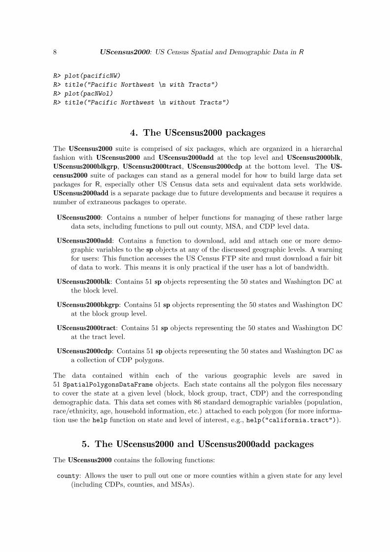
R> plot(pacificNW)
R> title("Pacific Northwest \n with Tracts")
R> plot(pacNWol)
R> title("Pacific Northwest \n without Tracts")
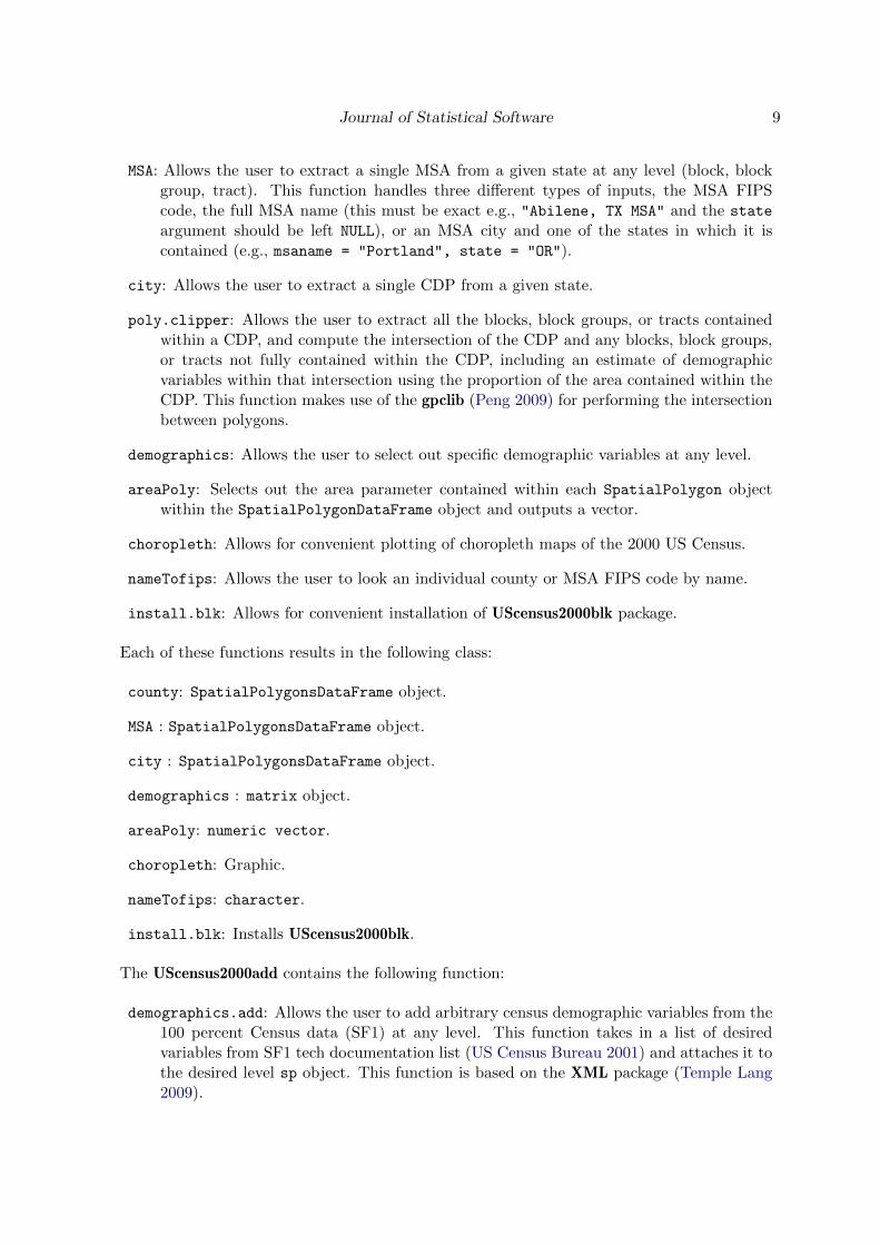
4. The UScensus2000 packages
The UScensus2000 suite is comprised of six packages, which are organized in a hierarchalfashion with UScensus2000 and UScensus2000add at the top level and UScensus2000blk,UScensus2000blkgrp, UScensus2000tract, UScensus2000cdp at the bottom level. The US-census2000 suite of packages can stand as a general model for how to build large data setpackages for R, especially other US Census data sets and equivalent data sets worldwide.UScensus2000add is a separate package due to future developments and because it requires anumber of extraneous packages to operate.
UScensus2000: Contains a number of helper functions for managing of these rather largedata sets, including functions to pull out county, MSA, and CDP level data.
UScensus2000add: Contains a function to download, add and attach one or more demo-graphic variables to the sp objects at any of the discussed geographic levels. A warningfor users: This function accesses the US Census FTP site and must download a fair bitof data to work. This means it is only practical if the user has a lot of bandwidth.
UScensus2000blk: Contains 51 sp objects representing the 50 states and Washington DC atthe block level.
UScensus2000bkgrp: Contains 51 sp objects representing the 50 states and Washington DCat the block group level.
UScensus2000tract: Contains 51 sp objects representing the 50 states and Washington DCat the tract level.
UScensus2000cdp: Contains 51 sp objects representing the 50 states and Washington DC asa collection of CDP polygons.
The data contained within each of the various geographic levels are saved in51 SpatialPolygonsDataFrame objects. Each state contains all the polygon files necessaryto cover the state at a given level (block, block group, tract, CDP) and the correspondingdemographic data. This data set comes with 86 standard demographic variables (population,race/ethnicity, age, household information, etc.) attached to each polygon (for more informa-tion use the help function on state and level of interest, e.g., help("california.tract")).
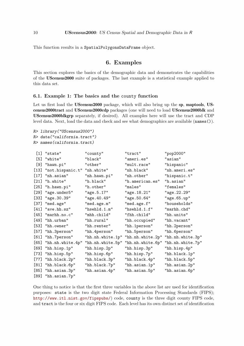
5. The UScensus2000 and UScensus2000add packages
The UScensus2000 contains the following functions:
county: Allows the user to pull out one or more counties within a given state for any level(including CDPs, counties, and MSAs).
Journal of Statistical Software 9
MSA: Allows the user to extract a single MSA from a given state at any level (block, blockgroup, tract). This function handles three different types of inputs, the MSA FIPScode, the full MSA name (this must be exact e.g., "Abilene, TX MSA" and the state
argument should be left NULL), or an MSA city and one of the states in which it iscontained (e.g., msaname = "Portland", state = "OR").
city: Allows the user to extract a single CDP from a given state.
poly.clipper: Allows the user to extract all the blocks, block groups, or tracts containedwithin a CDP, and compute the intersection of the CDP and any blocks, block groups,or tracts not fully contained within the CDP, including an estimate of demographicvariables within that intersection using the proportion of the area contained within theCDP. This function makes use of the gpclib (Peng 2009) for performing the intersectionbetween polygons.
demographics: Allows the user to select out specific demographic variables at any level.
areaPoly: Selects out the area parameter contained within each SpatialPolygon objectwithin the SpatialPolygonDataFrame object and outputs a vector.
choropleth: Allows for convenient plotting of choropleth maps of the 2000 US Census.
nameTofips: Allows the user to look an individual county or MSA FIPS code by name.
install.blk: Allows for convenient installation of UScensus2000blk package.
Each of these functions results in the following class:
county: SpatialPolygonsDataFrame object.
MSA : SpatialPolygonsDataFrame object.
city : SpatialPolygonsDataFrame object.
demographics : matrix object.
areaPoly: numeric vector.
choropleth: Graphic.
nameTofips: character.
install.blk: Installs UScensus2000blk.
The UScensus2000add contains the following function:
demographics.add: Allows the user to add arbitrary census demographic variables from the100 percent Census data (SF1) at any level. This function takes in a list of desiredvariables from SF1 tech documentation list (US Census Bureau 2001) and attaches it tothe desired level sp object. This function is based on the XML package (Temple Lang2009).
10 UScensus2000: US Census Spatial and Demographic Data in R
This function results in a SpatialPolygonsDataFrame object.
6. Examples
This section explores the basics of the demographic data and demonstrates the capabilitiesof the UScensus2000 suite of packages. The last example is a statistical example applied tothis data set.
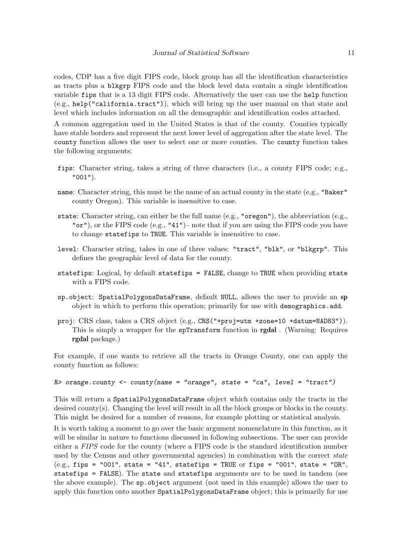
6.1. Example 1: The basics and the county function
Let us first load the UScensus2000 package, which will also bring up the sp, maptools, US-census2000tract and UScensus2000cdp packages (one will need to load UScensus2000blk andUScensus2000blkgrp separately, if desired). All examples here will use the tract and CDPlevel data. Next, load the data and check and see what demographics are available (names()).
R> library("UScensus2000")
R> data("california.tract")
R> names(california.tract)
[1] "state" "county" "tract" "pop2000"
[5] "white" "black" "ameri.es" "asian"
[9] "hawn.pi" "other" "mult.race" "hispanic"
[13] "not.hispanic.t" "nh.white" "nh.black" "nh.ameri.es"
[17] "nh.asian" "nh.hawn.pi" "nh.other" "hispanic.t"
[21] "h.white" "h.black" "h.american.es" "h.asian"
[25] "h.hawn.pi" "h.other" "males" "females"
[29] "age.under5" "age.5.17" "age.18.21" "age.22.29"
[33] "age.30.39" "age.40.49" "age.50.64" "age.65.up"
[37] "med.age" "med.age.m" "med.age.f" "households"
[41] "ave.hh.sz" "hsehld.1.m" "hsehld.1.f" "marhh.chd"
[45] "marhh.no.c" "mhh.child" "fhh.child" "hh.units"
[49] "hh.urban" "hh.rural" "hh.occupied" "hh.vacant"
[53] "hh.owner" "hh.renter" "hh.1person" "hh.2person"
[57] "hh.3person" "hh.4person" "hh.5person" "hh.6person"
[61] "hh.7person" "hh.nh.white.1p" "hh.nh.white.2p" "hh.nh.white.3p"
[65] "hh.nh.white.4p" "hh.nh.white.5p" "hh.nh.white.6p" "hh.nh.white.7p"
[69] "hh.hisp.1p" "hh.hisp.2p" "hh.hisp.3p" "hh.hisp.4p"
[73] "hh.hisp.5p" "hh.hisp.6p" "hh.hisp.7p" "hh.black.1p"
[77] "hh.black.2p" "hh.black.3p" "hh.black.4p" "hh.black.5p"
[81] "hh.black.6p" "hh.black.7p" "hh.asian.1p" "hh.asian.2p"
[85] "hh.asian.3p" "hh.asian.4p" "hh.asian.5p" "hh.asian.6p"
[89] "hh.asian.7p"
One thing to notice is that the first three variables in the above list are used for identificationpurposes: state is the two digit state Federal Information Processing Standards (FIPS);http://www.itl.nist.gov/fipspubs/) code, county is the three digit county FIPS code,and tract is the four or six digit FIPS code. Each level has its own distinct set of identification
Journal of Statistical Software 11
codes, CDP has a five digit FIPS code, block group has all the identification characteristicsas tracts plus a blkgrp FIPS code and the block level data contain a single identificationvariable fips that is a 13 digit FIPS code. Alternatively the user can use the help function(e.g., help("california.tract")), which will bring up the user manual on that state andlevel which includes information on all the demographic and identification codes attached.
A common aggregation used in the United States is that of the county. Counties typicallyhave stable borders and represent the next lower level of aggregation after the state level. Thecounty function allows the user to select one or more counties. The county function takesthe following arguments:
fips: Character string, takes a string of three characters (i.e., a county FIPS code; e.g.,"001").
name: Character string, this must be the name of an actual county in the state (e.g., "Baker"county Oregon). This variable is insensitive to case.
state: Character string, can either be the full name (e.g., "oregon"), the abbreviation (e.g.,"or"), or the FIPS code (e.g., "41")– note that if you are using the FIPS code you haveto change statefips to TRUE. This variable is insensitive to case.
level: Character string, takes in one of three values: "tract", "blk", or "blkgrp". Thisdefines the geographic level of data for the county.
statefips: Logical, by default statefips = FALSE, change to TRUE when providing state
with a FIPS code.
sp.object: SpatialPolygonsDataFrame, default NULL, allows the user to provide an spobject in which to perform this operation; primarily for use with demographics.add.
proj: CRS class, takes a CRS object (e.g., CRS("+proj=utm +zone=10 +datum=NAD83")).This is simply a wrapper for the spTransform function in rgdal . (Warning: Requiresrgdal package.)
For example, if one wants to retrieve all the tracts in Orange County, one can apply thecounty function as follows:
R> orange.county <- county(name = "orange", state = "ca", level = "tract")
This will return a SpatialPolygonsDataFrame object which contains only the tracts in thedesired county(s). Changing the level will result in all the block groups or blocks in the county.This might be desired for a number of reasons, for example plotting or statistical analysis.
It is worth taking a moment to go over the basic argument nomenclature in this function, as itwill be similar in nature to functions discussed in following subsections. The user can provideeither a FIPS code for the county (where a FIPS code is the standard identification numberused by the Census and other governmental agencies) in combination with the correct state(e.g., fips = "001", state = "41", statefips = TRUE or fips = "001", state = "OR",statefips = FALSE). The state and statefips arguments are to be used in tandem (seethe above example). The sp.object argument (not used in this example) allows the user toapply this function onto another SpatialPolygonsDataFrame object; this is primarily for use
12 UScensus2000: US Census Spatial and Demographic Data in R
with the demographics.add function discussed in section 6.6 (an example is also provided).The proj argument (not discussed in this article) allows the user to re-project the datausing the spTransform function provided in the rgdal package (Keitt, Bivand, Pebesma, andRowlingson 2009).
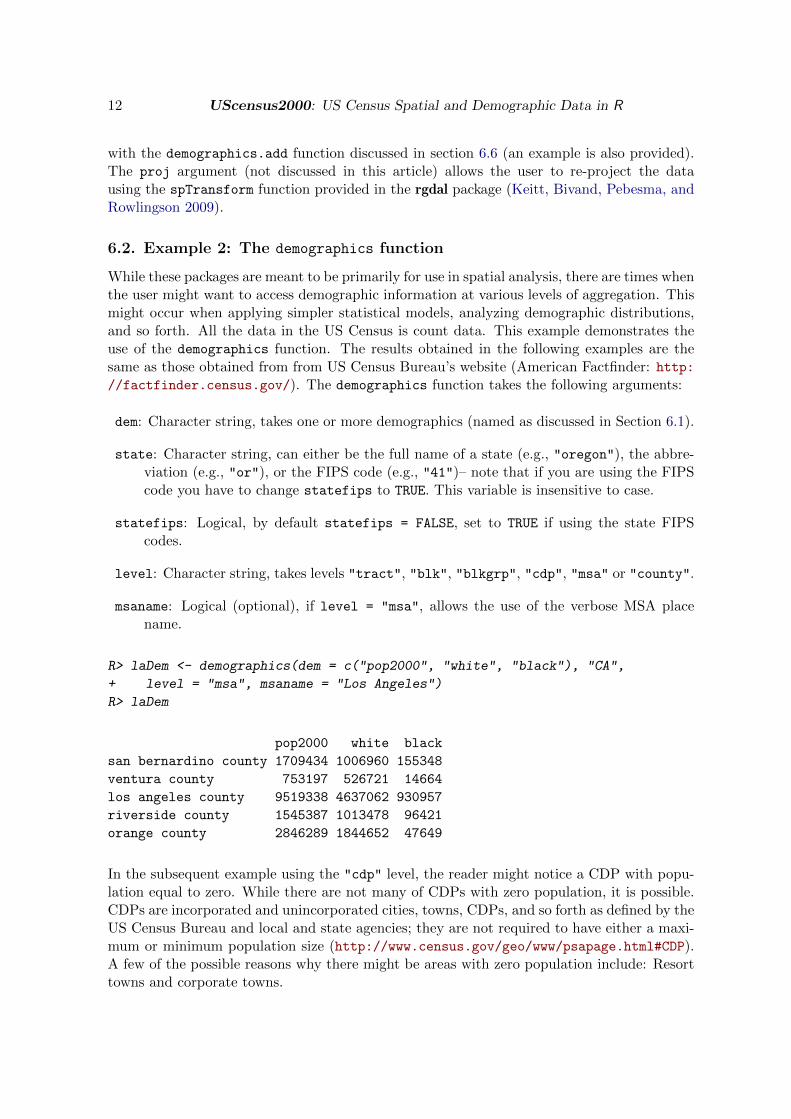
6.2. Example 2: The demographics function
While these packages are meant to be primarily for use in spatial analysis, there are times whenthe user might want to access demographic information at various levels of aggregation. Thismight occur when applying simpler statistical models, analyzing demographic distributions,and so forth. All the data in the US Census is count data. This example demonstrates theuse of the demographics function. The results obtained in the following examples are thesame as those obtained from from US Census Bureau’s website (American Factfinder: http://factfinder.census.gov/). The demographics function takes the following arguments:
dem: Character string, takes one or more demographics (named as discussed in Section 6.1).
state: Character string, can either be the full name of a state (e.g., "oregon"), the abbre-viation (e.g., "or"), or the FIPS code (e.g., "41")– note that if you are using the FIPScode you have to change statefips to TRUE. This variable is insensitive to case.
statefips: Logical, by default statefips = FALSE, set to TRUE if using the state FIPScodes.
level: Character string, takes levels "tract", "blk", "blkgrp", "cdp", "msa" or "county".
msaname: Logical (optional), if level = "msa", allows the use of the verbose MSA placename.
R> laDem <- demographics(dem = c("pop2000", "white", "black"), "CA",
+ level = "msa", msaname = "Los Angeles")
R> laDem
pop2000 white black
san bernardino county 1709434 1006960 155348
ventura county 753197 526721 14664
los angeles county 9519338 4637062 930957
riverside county 1545387 1013478 96421
orange county 2846289 1844652 47649
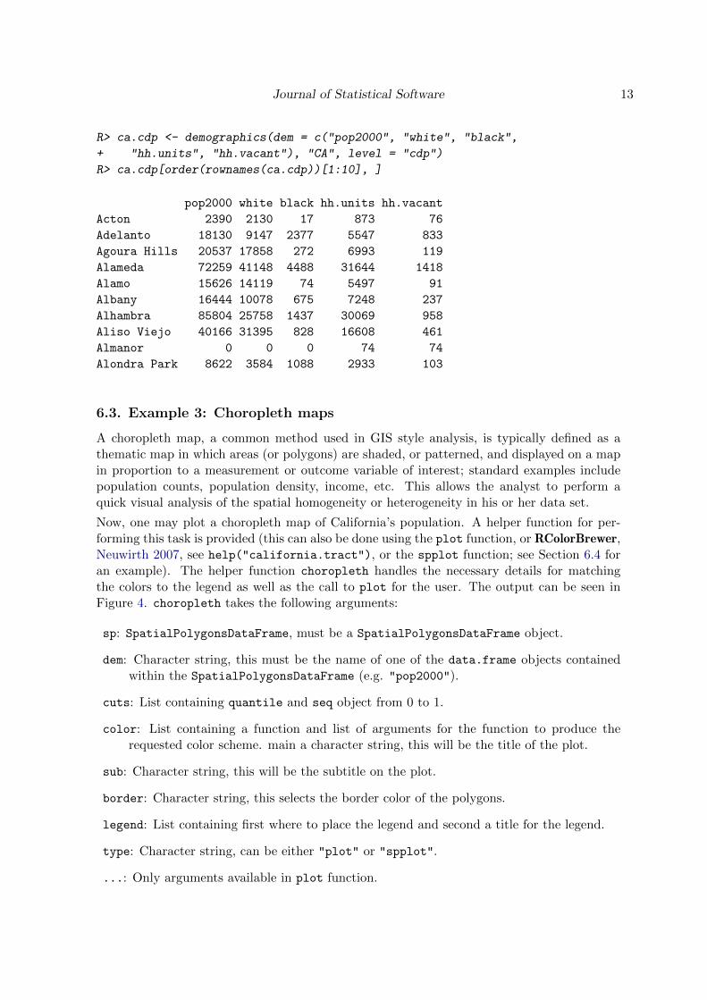
In the subsequent example using the "cdp" level, the reader might notice a CDP with popu-lation equal to zero. While there are not many of CDPs with zero population, it is possible.CDPs are incorporated and unincorporated cities, towns, CDPs, and so forth as defined by theUS Census Bureau and local and state agencies; they are not required to have either a maxi-mum or minimum population size (http://www.census.gov/geo/www/psapage.html#CDP).A few of the possible reasons why there might be areas with zero population include: Resorttowns and corporate towns.
Journal of Statistical Software 13
R> ca.cdp <- demographics(dem = c("pop2000", "white", "black",
+ "hh.units", "hh.vacant"), "CA", level = "cdp")
R> ca.cdp[order(rownames(ca.cdp))[1:10], ]
pop2000 white black hh.units hh.vacant
Acton 2390 2130 17 873 76
Adelanto 18130 9147 2377 5547 833
Agoura Hills 20537 17858 272 6993 119
Alameda 72259 41148 4488 31644 1418
Alamo 15626 14119 74 5497 91
Albany 16444 10078 675 7248 237
Alhambra 85804 25758 1437 30069 958
Aliso Viejo 40166 31395 828 16608 461
Almanor 0 0 0 74 74
Alondra Park 8622 3584 1088 2933 103
6.3. Example 3: Choropleth maps
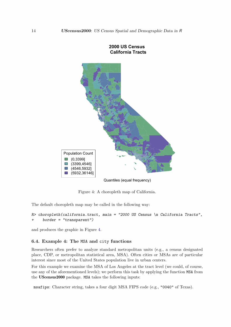
A choropleth map, a common method used in GIS style analysis, is typically defined as athematic map in which areas (or polygons) are shaded, or patterned, and displayed on a mapin proportion to a measurement or outcome variable of interest; standard examples includepopulation counts, population density, income, etc. This allows the analyst to perform aquick visual analysis of the spatial homogeneity or heterogeneity in his or her data set.
Now, one may plot a choropleth map of California’s population. A helper function for per-forming this task is provided (this can also be done using the plot function, or RColorBrewer,Neuwirth 2007, see help("california.tract"), or the spplot function; see Section 6.4 foran example). The helper function choropleth handles the necessary details for matchingthe colors to the legend as well as the call to plot for the user. The output can be seen inFigure 4. choropleth takes the following arguments:
sp: SpatialPolygonsDataFrame, must be a SpatialPolygonsDataFrame object.
dem: Character string, this must be the name of one of the data.frame objects containedwithin the SpatialPolygonsDataFrame (e.g. "pop2000").
cuts: List containing quantile and seq object from 0 to 1.
color: List containing a function and list of arguments for the function to produce therequested color scheme. main a character string, this will be the title of the plot.
sub: Character string, this will be the subtitle on the plot.
border: Character string, this selects the border color of the polygons.
legend: List containing first where to place the legend and second a title for the legend.
type: Character string, can be either "plot" or "spplot".
...: Only arguments available in plot function.
14 UScensus2000: US Census Spatial and Demographic Data in R
Figure 4: A choropleth map of California.
The default choropleth map may be called in the following way:
R> choropleth(california.tract, main = "2000 US Census \n California Tracts",
+ border = "transparent")
and produces the graphic in Figure 4.
6.4. Example 4: The MSA and city functions
Researchers often prefer to analyze standard metropolitan units (e.g., a census designatedplace, CDP, or metropolitan statistical area, MSA). Often cities or MSAs are of particularinterest since most of the United States population live in urban centers.
For this example we examine the MSA of Los Angeles at the tract level (we could, of course,use any of the aforementioned levels); we perform this task by applying the function MSA fromthe UScensus2000 package. MSA takes the following inputs:
msafips: Character string, takes a four digit MSA FIPS code (e.g., "0040" of Texas).
Journal of Statistical Software 15
msaname: Character string, this can either be in conjunction with the variable state or not.Case 1: Full MSA name (state should be left NULL in this case, e.g., "Abilene, TX
MSA"); this must be exact. Case 2: Takes one of the city names of the MSA and the oneof the states which contain the MSA (e.g., msaname = "Albany" and state = "NY").
state: Character string, can either be the full name (e.g., "oregon"), the abbreviation (e.g.,"or"), or the FIPS code (e.g., "41"). Note that if you are using the FIPS code youhave to change statefips to TRUE. This variable is insensitive to case. This is used inconjunction with msaname, see above for more details.
statefips: Logical, by default statefips = FALSE, change to TRUE when providing state
with a FIPS code. msaname must also be a FIPS code when using this mode.
level: Character string, takes in one of three values: "tract", "blk", or "blkgrp". Thisdefines the geographic level of data for the MSA.
proj: CRS class, takes a CRS object (e.g., CRS("+proj=utm +zone=10 +datum=NAD83")).This is simply a wrapper for the spTransform function in rgdal. (Warning: Requiresrgdal package.)
To plot the boundary of Los Angeles proper on top of this MSA area we will use the followingfunction: city, also from the UScensus2000 package. The output can be seen in Figure 5.city takes the following inputs:
name: Character string, takes the value of a string or string vector and has to be the exactname or names of CDP(s). (If you are unsure of the exact name a quick way to findit is to load the library("UScensus2000cdp") and pull out the list of names for thestate you are interested in (see example below).
state: Character string, can either be the full name (e.g., "oregon"), the abbreviation (e.g.,"or"), or the FIPS code (e.g., "41")– note that if you are using the FIPS code you haveto change statefips to TRUE. This variable is insensitive to case.
statefips: Logical, by default statefips = FALSE, change to TRUE when providing state
with a FIPS code. name must also be a FIPS code when using this mode.
sp.object: SpatialPolygonsDataFrame, default NULL, allows the user to provide an spobject in which to perform this operation; primarily for use with demographics.add
function.
proj: CRS class, takes a CRS object (e.g., CRS("+proj=utm +zone=10 +datum=NAD83")).This is simply a wrapper for the spTransform function in rgdal. (Warning: Requiresrgdal package.)
Let us breakdown these two functions. MSA has three main ways of extracting a specified MSA:By using the five digit MSA FIPS code via the variable msafips (not used in this example);by supplying the full MSA name to msaname (e.g., "Portland-Salem, OR-WA CMSA"); or byproviding the name of one of the cities from the full name of the MSA (e.g., "Portland") andone of the state abbreviations from the full MSA name or one of the state FIPS codes (e.g.,"OR") in the state argument. The level argument specifies the geographical level and can
16 UScensus2000: US Census Spatial and Demographic Data in R
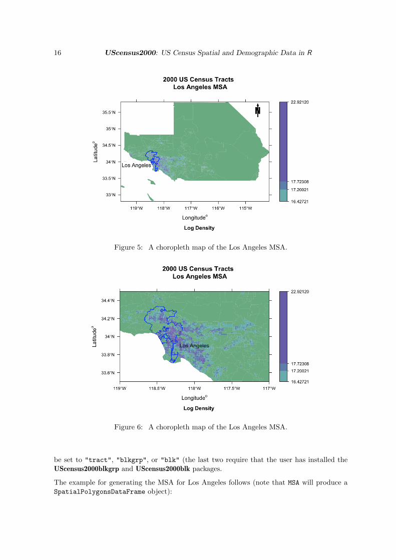
Figure 5: A choropleth map of the Los Angeles MSA.
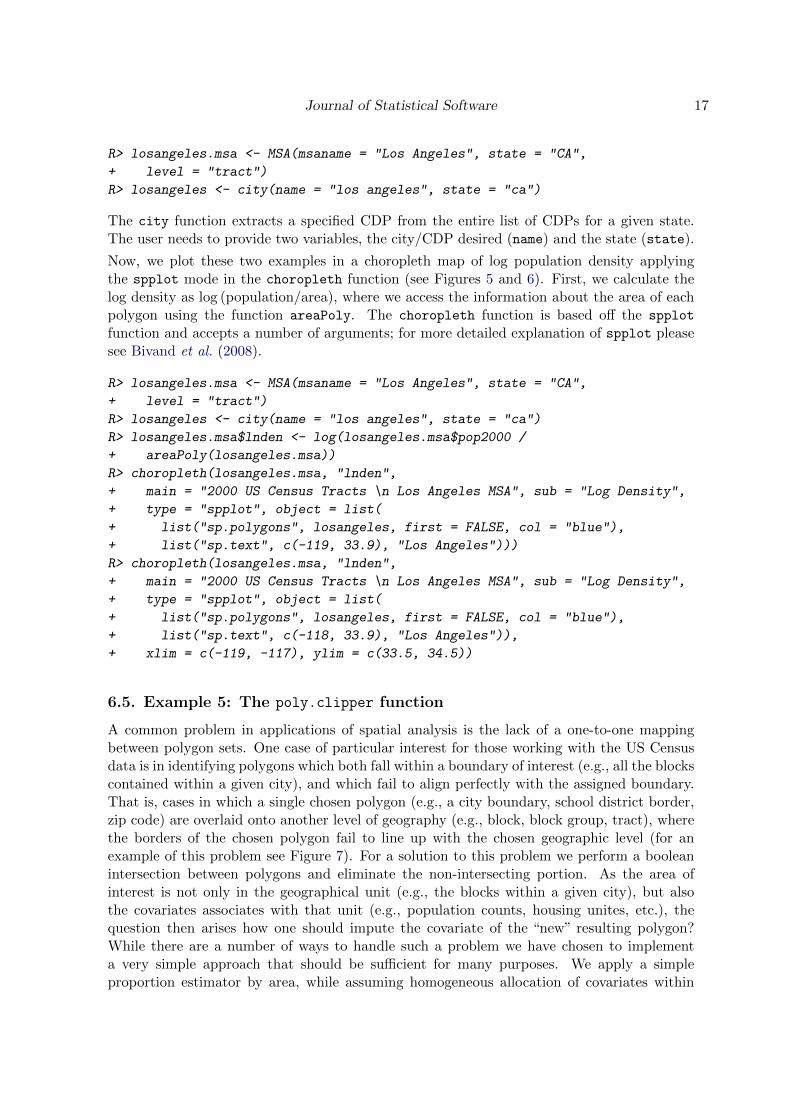
Figure 6: A choropleth map of the Los Angeles MSA.
be set to "tract", "blkgrp", or "blk" (the last two require that the user has installed theUScensus2000blkgrp and UScensus2000blk packages.
The example for generating the MSA for Los Angeles follows (note that MSA will produce aSpatialPolygonsDataFrame object):
Journal of Statistical Software 17
R> losangeles.msa <- MSA(msaname = "Los Angeles", state = "CA",
+ level = "tract")
R> losangeles <- city(name = "los angeles", state = "ca")
The city function extracts a specified CDP from the entire list of CDPs for a given state.The user needs to provide two variables, the city/CDP desired (name) and the state (state).
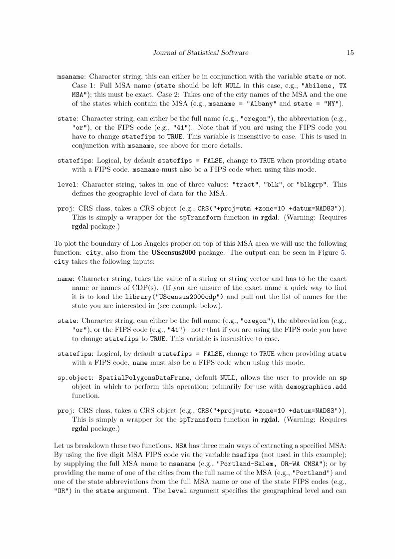
Now, we plot these two examples in a choropleth map of log population density applyingthe spplot mode in the choropleth function (see Figures 5 and 6). First, we calculate thelog density as log (population/area), where we access the information about the area of eachpolygon using the function areaPoly. The choropleth function is based off the spplot
function and accepts a number of arguments; for more detailed explanation of spplot pleasesee Bivand et al. (2008).
R> losangeles.msa <- MSA(msaname = "Los Angeles", state = "CA",
+ level = "tract")
R> losangeles <- city(name = "los angeles", state = "ca")
R> losangeles.msa$lnden <- log(losangeles.msa$pop2000 /
+ areaPoly(losangeles.msa))
R> choropleth(losangeles.msa, "lnden",
+ main = "2000 US Census Tracts \n Los Angeles MSA", sub = "Log Density",
+ type = "spplot", object = list(
+ list("sp.polygons", losangeles, first = FALSE, col = "blue"),
+ list("sp.text", c(-119, 33.9), "Los Angeles")))
R> choropleth(losangeles.msa, "lnden",
+ main = "2000 US Census Tracts \n Los Angeles MSA", sub = "Log Density",
+ type = "spplot", object = list(
+ list("sp.polygons", losangeles, first = FALSE, col = "blue"),
+ list("sp.text", c(-118, 33.9), "Los Angeles")),
+ xlim = c(-119, -117), ylim = c(33.5, 34.5))
6.5. Example 5: The poly.clipper function
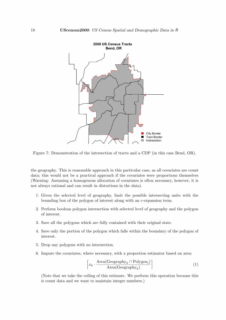
A common problem in applications of spatial analysis is the lack of a one-to-one mappingbetween polygon sets. One case of particular interest for those working with the US Censusdata is in identifying polygons which both fall within a boundary of interest (e.g., all the blockscontained within a given city), and which fail to align perfectly with the assigned boundary.That is, cases in which a single chosen polygon (e.g., a city boundary, school district border,zip code) are overlaid onto another level of geography (e.g., block, block group, tract), wherethe borders of the chosen polygon fail to line up with the chosen geographic level (for anexample of this problem see Figure 7). For a solution to this problem we perform a booleanintersection between polygons and eliminate the non-intersecting portion. As the area ofinterest is not only in the geographical unit (e.g., the blocks within a given city), but alsothe covariates associates with that unit (e.g., population counts, housing unites, etc.), thequestion then arises how one should impute the covariate of the “new” resulting polygon?While there are a number of ways to handle such a problem we have chosen to implementa very simple approach that should be sufficient for many purposes. We apply a simpleproportion estimator by area, while assuming homogeneous allocation of covariates within
18 UScensus2000: US Census Spatial and Demographic Data in R
Figure 7: Demonstration of the intersection of tracts and a CDP (in this case Bend, OR).
the geography. This is reasonable approach in this particular case, as all covariates are countdata; this would not be a practical approach if the covariates were proportions themselves(Warning: Assuming a homogenous allocation of covariates is often necessary, however, it isnot always rational and can result in distortions in the data).
1. Given the selected level of geography, limit the possible intersecting units with thebounding box of the polygon of interest along with an ε-expansion term.
2. Perform boolean polygon intersection with selected level of geography and the polygonof interest.
3. Save all the polygons which are fully contained with their original state.
4. Save only the portion of the polygon which falls within the boundary of the polygon ofinterest.
5. Drop any polygons with no intersection.
6. Impute the covariates, where necessary, with a proportion estimator based on area:⌈xk ·
Area(Geographyk ∩ Polygoni)
Area(Geographyk)
⌉(1)
(Note that we take the ceiling of this estimate. We perform this operation because thisis count data and we want to maintain integer numbers.)
Journal of Statistical Software 19
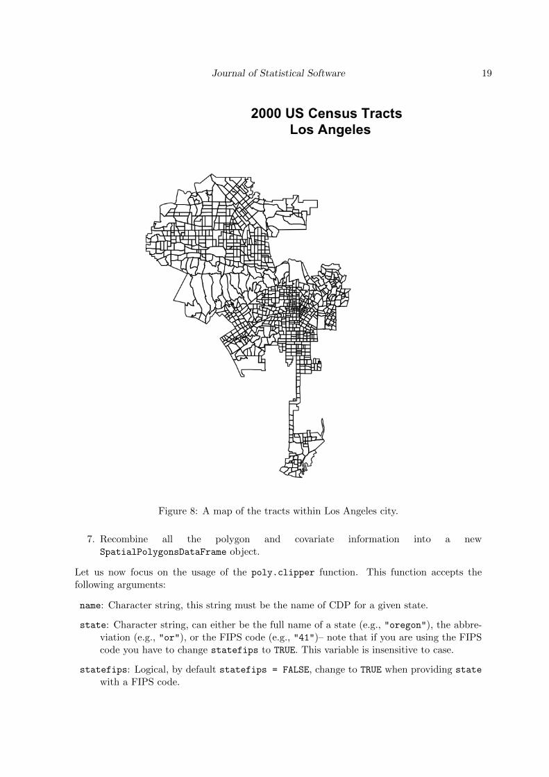
Figure 8: A map of the tracts within Los Angeles city.
7. Recombine all the polygon and covariate information into a newSpatialPolygonsDataFrame object.
Let us now focus on the usage of the poly.clipper function. This function accepts thefollowing arguments:
name: Character string, this string must be the name of CDP for a given state.
state: Character string, can either be the full name of a state (e.g., "oregon"), the abbre-viation (e.g., "or"), or the FIPS code (e.g., "41")– note that if you are using the FIPScode you have to change statefips to TRUE. This variable is insensitive to case.
statefips: Logical, by default statefips = FALSE, change to TRUE when providing state
with a FIPS code.
20 UScensus2000: US Census Spatial and Demographic Data in R
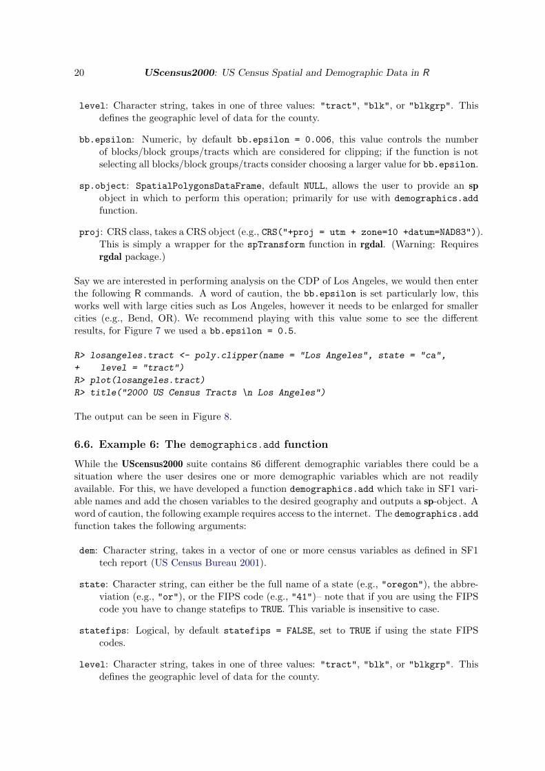
level: Character string, takes in one of three values: "tract", "blk", or "blkgrp". Thisdefines the geographic level of data for the county.
bb.epsilon: Numeric, by default bb.epsilon = 0.006, this value controls the numberof blocks/block groups/tracts which are considered for clipping; if the function is notselecting all blocks/block groups/tracts consider choosing a larger value for bb.epsilon.
sp.object: SpatialPolygonsDataFrame, default NULL, allows the user to provide an spobject in which to perform this operation; primarily for use with demographics.add
function.
proj: CRS class, takes a CRS object (e.g., CRS("+proj = utm + zone=10 +datum=NAD83")).This is simply a wrapper for the spTransform function in rgdal. (Warning: Requiresrgdal package.)
Say we are interested in performing analysis on the CDP of Los Angeles, we would then enterthe following R commands. A word of caution, the bb.epsilon is set particularly low, thisworks well with large cities such as Los Angeles, however it needs to be enlarged for smallercities (e.g., Bend, OR). We recommend playing with this value some to see the differentresults, for Figure 7 we used a bb.epsilon = 0.5.
R> losangeles.tract <- poly.clipper(name = "Los Angeles", state = "ca",
+ level = "tract")
R> plot(losangeles.tract)
R> title("2000 US Census Tracts \n Los Angeles")
The output can be seen in Figure 8.
6.6. Example 6: The demographics.add function
While the UScensus2000 suite contains 86 different demographic variables there could be asituation where the user desires one or more demographic variables which are not readilyavailable. For this, we have developed a function demographics.add which take in SF1 vari-able names and add the chosen variables to the desired geography and outputs a sp-object. Aword of caution, the following example requires access to the internet. The demographics.addfunction takes the following arguments:
dem: Character string, takes in a vector of one or more census variables as defined in SF1tech report (US Census Bureau 2001).
state: Character string, can either be the full name of a state (e.g., "oregon"), the abbre-viation (e.g., "or"), or the FIPS code (e.g., "41")– note that if you are using the FIPScode you have to change statefips to TRUE. This variable is insensitive to case.
statefips: Logical, by default statefips = FALSE, set to TRUE if using the state FIPScodes.
level: Character string, takes in one of three values: "tract", "blk", or "blkgrp". Thisdefines the geographic level of data for the county.
Journal of Statistical Software 21
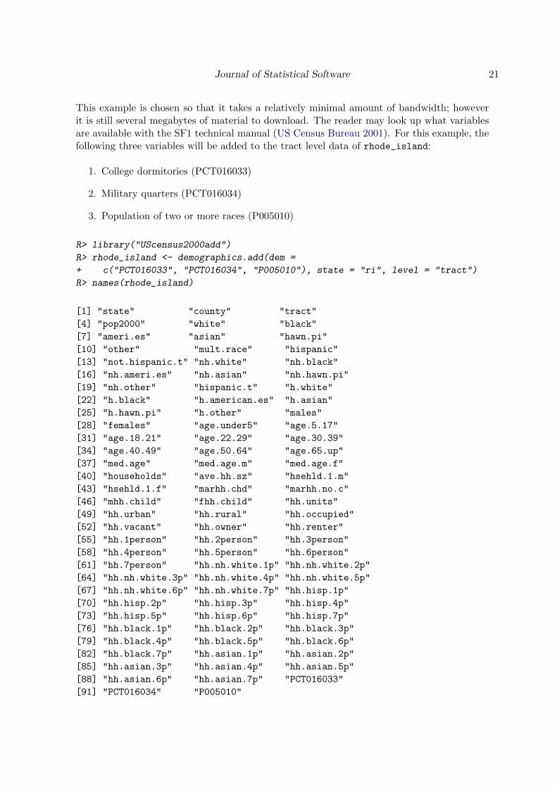
This example is chosen so that it takes a relatively minimal amount of bandwidth; howeverit is still several megabytes of material to download. The reader may look up what variablesare available with the SF1 technical manual (US Census Bureau 2001). For this example, thefollowing three variables will be added to the tract level data of rhode_island:
1. College dormitories (PCT016033)
2. Military quarters (PCT016034)
3. Population of two or more races (P005010)
R> library("UScensus2000add")
R> rhode_island <- demographics.add(dem =
+ c("PCT016033", "PCT016034", "P005010"), state = "ri", level = "tract")
R> names(rhode_island)
[1] "state" "county" "tract"
[4] "pop2000" "white" "black"
[7] "ameri.es" "asian" "hawn.pi"
[10] "other" "mult.race" "hispanic"
[13] "not.hispanic.t" "nh.white" "nh.black"
[16] "nh.ameri.es" "nh.asian" "nh.hawn.pi"
[19] "nh.other" "hispanic.t" "h.white"
[22] "h.black" "h.american.es" "h.asian"
[25] "h.hawn.pi" "h.other" "males"
[28] "females" "age.under5" "age.5.17"
[31] "age.18.21" "age.22.29" "age.30.39"
[34] "age.40.49" "age.50.64" "age.65.up"
[37] "med.age" "med.age.m" "med.age.f"
[40] "households" "ave.hh.sz" "hsehld.1.m"
[43] "hsehld.1.f" "marhh.chd" "marhh.no.c"
[46] "mhh.child" "fhh.child" "hh.units"
[49] "hh.urban" "hh.rural" "hh.occupied"
[52] "hh.vacant" "hh.owner" "hh.renter"
[55] "hh.1person" "hh.2person" "hh.3person"
[58] "hh.4person" "hh.5person" "hh.6person"
[61] "hh.7person" "hh.nh.white.1p" "hh.nh.white.2p"
[64] "hh.nh.white.3p" "hh.nh.white.4p" "hh.nh.white.5p"
[67] "hh.nh.white.6p" "hh.nh.white.7p" "hh.hisp.1p"
[70] "hh.hisp.2p" "hh.hisp.3p" "hh.hisp.4p"
[73] "hh.hisp.5p" "hh.hisp.6p" "hh.hisp.7p"
[76] "hh.black.1p" "hh.black.2p" "hh.black.3p"
[79] "hh.black.4p" "hh.black.5p" "hh.black.6p"
[82] "hh.black.7p" "hh.asian.1p" "hh.asian.2p"
[85] "hh.asian.3p" "hh.asian.4p" "hh.asian.5p"
[88] "hh.asian.6p" "hh.asian.7p" "PCT016033"
[91] "PCT016034" "P005010"
22 UScensus2000: US Census Spatial and Demographic Data in R
Now that we have added the demographics: PCT016033, PCT016034, P005010, we can buildan sp object of Providence, RI from this object with the following command
R> providence <- poly.clipper(name = "providence", state = "RI",
+ level = "tract", sp.object = rhode_island)
There is only a small difference between this code and that from Section 6.5; the sp.object
= rhode_island argument. The sp.object tells the poly.clipper function to use therhode_island object for the base of the clipping; this has the added benefit of perform-ing the proportion estimator to the newly added demographics. A word of caution if one addsa covariate to the sp object which is not of a count type variable (e.g., a ratio), the resultingestimation performed should be ignored.
6.7. Example 7: A statistical application of the UScensus2000 suite
The last example is a statistical example based on the spdep package (Bivand 2009) andmotivated by the example given in Bivand et al. (2008, Section 10.2). It will walk the readerthrough using this data in performing a common model based approach for handling spatialautocorrelation.
There are many different possible models for spatial autocorrelation, however one of the mostused in practice is that of the simultaneous autoregressive (SAR) models (Bivand et al. 2008).These are models of the form Y = WY + µ+ e, where W is a weight matrix, µ is estimatedwith the standard linear model (µ = X>β) and e is assumed to be distributed N(0, σ2). Oneway to think about this model is to assume that the observations arise from the equilibriumof a linear diffusion process with a weight matrix W and initial state vector µ+ e.
Say one is interested in modeling the percent of home owners in a given tract in Los Angeles.There is a long history of the study of segregation and inequality in neighborhoods (Masseyand Fong 1990; Massey and Denton 1988a,b, 1993) much of which suggest the hypothesisthat we will see lower home ownership rates in minority tracts. One might endeavor to modelthis hypothesis by adding covariates for race/ethnicity in the form of: Percent non-hispanicwhite, non-hispanic black, non-hispanic asian, and hispanic, where we would expect to seea positive effect for non-hispanic white (i.e., increase in home ownership) and a decrease forall minorities. Another potential hypothesis is that families with children are more likely toown houses, so we might propose the hypothesis that the percentage of married householdswith children should increase the likelihood of home ownership. We could test this by addinga covariate for the percent of married families with children. To confirm our hypothesis weshould see a positive effect.
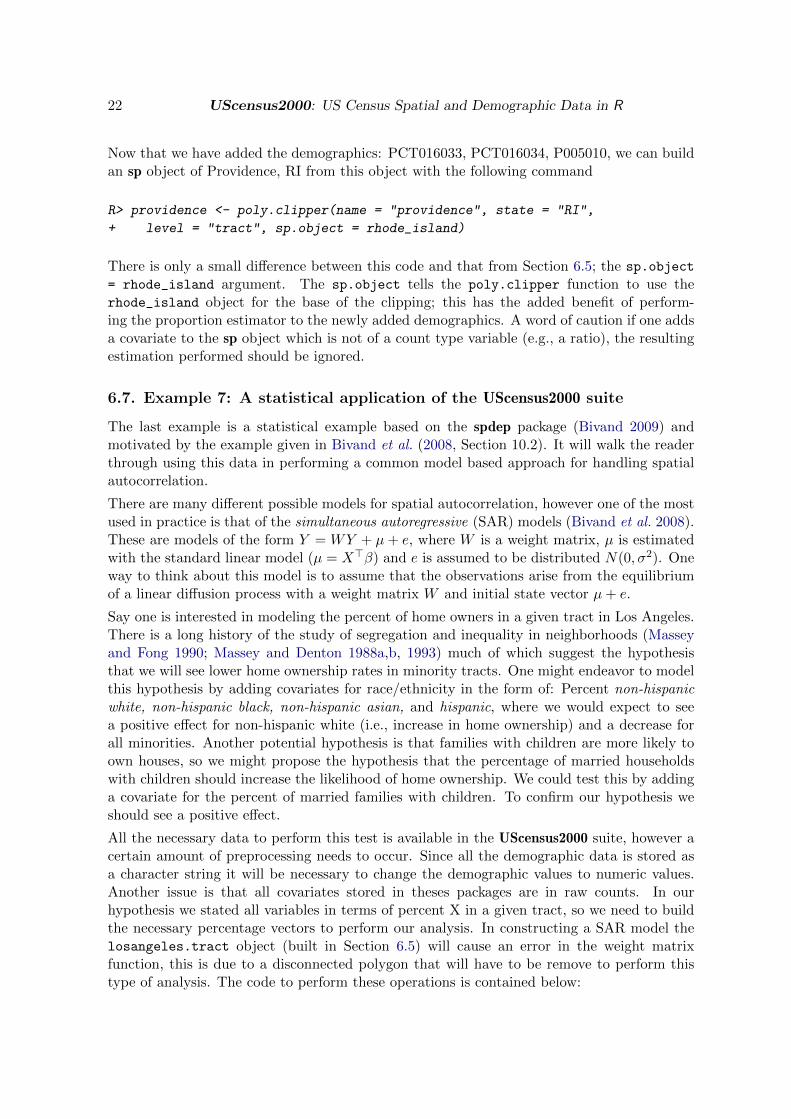
All the necessary data to perform this test is available in the UScensus2000 suite, however acertain amount of preprocessing needs to occur. Since all the demographic data is stored asa character string it will be necessary to change the demographic values to numeric values.Another issue is that all covariates stored in theses packages are in raw counts. In ourhypothesis we stated all variables in terms of percent X in a given tract, so we need to buildthe necessary percentage vectors to perform our analysis. In constructing a SAR model thelosangeles.tract object (built in Section 6.5) will cause an error in the weight matrixfunction, this is due to a disconnected polygon that will have to be remove to perform thistype of analysis. The code to perform these operations is contained below:
Journal of Statistical Software 23
R> library("spdep")
R> la.pop.tot <- losangeles.tract$pop2000
R> la.hh.tot <- losangeles.tract$households
R> losangeles.tract$pctowner <- losangeles.tract$hh.owner/la.hh.tot
R> losangeles.tract$pct.nh.white <- losangeles.tract$nh.white/la.pop.tot
R> losangeles.tract$pct.nh.black <- losangeles.tract$nh.black/la.pop.tot
R> losangeles.tract$pct.hispanic <- losangeles.tract$hispanic/la.pop.tot
R> losangeles.tract$pct.nh.asian <- losangeles.tract$asian/la.pop.tot
R> losangeles.tract$pct.marhh.chd <- losangeles.tract$marhh.chd/la.hh.tot
R> losangeles.tract <- losangeles.tract[c(1:297,
+ 299:length(losangeles.tract@polygons)),]
To test our hypothesis a reasonable approach is to start by fitting a simple linear regressionmodel with the aforementioned covariates. We notice that we can treat theSpatialPolygonDataFrame objects just like the standard R data.frame object.
R> la.lm <- lm(pctowner ~ pct.nh.white + pct.hispanic + pct.nh.black +
+ pct.nh.asian + pct.marhh.chd, data = losangeles.tract)
R> summary(la.lm)
Call:
lm(formula = pctowner ~ pct.nh.white + pct.hispanic + pct.nh.black +
pct.nh.asian + pct.marhh.chd, data = losangeles.tract)
Residuals:
Min 1Q Median 3Q Max
-0.795045 -0.115970 -0.009655 0.106370 0.637660
Coefficients:
Estimate Std. Error t value Pr(>|t|)
(Intercept) 0.33941 0.02598 13.064 <2e-16 ***
pct.nh.white 0.04386 0.03791 1.157 0.248
pct.hispanic -0.80911 0.04686 -17.268 <2e-16 ***
pct.nh.black -0.04052 0.03621 -1.119 0.263
pct.nh.asian -0.46423 0.04723 -9.830 <2e-16 ***
pct.marhh.chd 1.87897 0.07207 26.071 <2e-16 ***
---
Signif. codes: 0 *** 0.001 ** 0.01 * 0.05 . 0.1 1
Residual standard error: 0.1747 on 881 degrees of freedom
(1 observation deleted due to missingness)
Multiple R-squared: 0.5945, Adjusted R-squared: 0.5922
F-statistic: 258.3 on 5 and 881 DF, p-value: < 2.2e-16
Looking at this standard linear regression we see that our initial race/ethnicity hypothesis ispartially confirmed (although, percentage non-hispanic white is not significant) and that ourmarried household with children hypothesis is also confirmed.
24 UScensus2000: US Census Spatial and Demographic Data in R
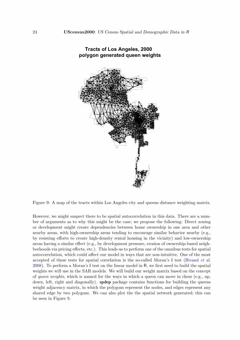
Figure 9: A map of the tracts within Los Angeles city and queens distance weighting matrix.
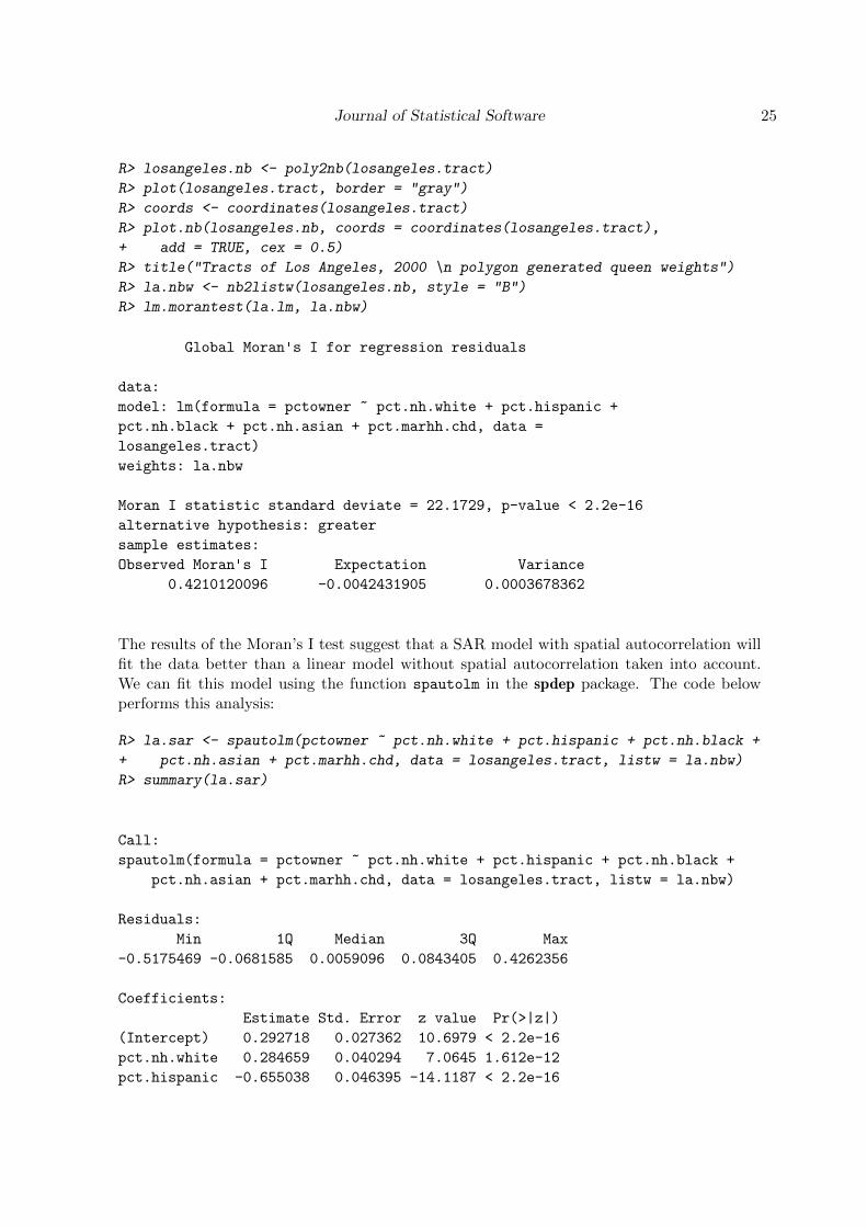
However, we might suspect there to be spatial autocorrelation in this data. There are a num-ber of arguments as to why this might be the case; we propose the following: Direct zoningor development might create dependencies between home ownership in one area and othernearby areas, with high-ownership areas tending to encourage similar behavior nearby (e.g.,by resisting efforts to create high-density rental housing in the vicinity) and low-ownershipareas having a similar effect (e.g., by development pressure, erosion of ownership-based neigh-borhoods via pricing effects, etc.). This leads us to perform one of the omnibus tests for spatialautocorrelation, which could affect our model in ways that are non-intuitive. One of the mostaccepted of these tests for spatial correlation is the so-called Moran’s I test (Bivand et al.2008). To perform a Moran’s I test on the linear model in R, we first need to build the spatialweights we will use in the SAR models. We will build our weight matrix based on the conceptof queen weights, which is named for the ways in which a queen can move in chess (e.g., up,down, left, right and diagonally). spdep package contains functions for building the queensweight adjacency matrix, in which the polygons represent the nodes, and edges represent anyshared edge by two polygons. We can also plot the the spatial network generated; this canbe seen in Figure 9.
Journal of Statistical Software 25
R> losangeles.nb <- poly2nb(losangeles.tract)
R> plot(losangeles.tract, border = "gray")
R> coords <- coordinates(losangeles.tract)
R> plot.nb(losangeles.nb, coords = coordinates(losangeles.tract),
+ add = TRUE, cex = 0.5)
R> title("Tracts of Los Angeles, 2000 \n polygon generated queen weights")
R> la.nbw <- nb2listw(losangeles.nb, style = "B")
R> lm.morantest(la.lm, la.nbw)
Global Moran's I for regression residuals
data:
model: lm(formula = pctowner ~ pct.nh.white + pct.hispanic +
pct.nh.black + pct.nh.asian + pct.marhh.chd, data =
losangeles.tract)
weights: la.nbw
Moran I statistic standard deviate = 22.1729, p-value < 2.2e-16
alternative hypothesis: greater
sample estimates:
Observed Moran's I Expectation Variance
0.4210120096 -0.0042431905 0.0003678362
The results of the Moran’s I test suggest that a SAR model with spatial autocorrelation willfit the data better than a linear model without spatial autocorrelation taken into account.We can fit this model using the function spautolm in the spdep package. The code belowperforms this analysis:
R> la.sar <- spautolm(pctowner ~ pct.nh.white + pct.hispanic + pct.nh.black +
+ pct.nh.asian + pct.marhh.chd, data = losangeles.tract, listw = la.nbw)
R> summary(la.sar)
Call:
spautolm(formula = pctowner ~ pct.nh.white + pct.hispanic + pct.nh.black +
pct.nh.asian + pct.marhh.chd, data = losangeles.tract, listw = la.nbw)
Residuals:
Min 1Q Median 3Q Max
-0.5175469 -0.0681585 0.0059096 0.0843405 0.4262356
Coefficients:
Estimate Std. Error z value Pr(>|z|)
(Intercept) 0.292718 0.027362 10.6979 < 2.2e-16
pct.nh.white 0.284659 0.040294 7.0645 1.612e-12
pct.hispanic -0.655038 0.046395 -14.1187 < 2.2e-16
26 UScensus2000: US Census Spatial and Demographic Data in R
pct.nh.black -0.049928 0.043829 -1.1392 0.2546
pct.nh.asian -0.276466 0.051743 -5.3430 9.140e-08
pct.marhh.chd 1.320579 0.071883 18.3712 < 2.2e-16
Lambda: 0.12459 LR test value: 394.72 p-value: < 2.22e-16
Log likelihood: 489.1817
ML residual variance (sigma squared): 0.01688, (sigma: 0.12992)
Number of observations: 887
Number of parameters estimated: 8
AIC: -962.36
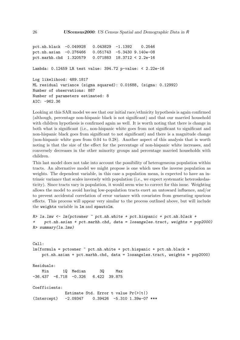
Looking at this SAR model we see that our initial race/ethnicity hypothesis is again confirmed(although, percentage non-hispanic black is not significant) and that our married householdwith children hypothesis is confirmed again as well. It is worth noting that there is change inboth what is significant (i.e., non-hispanic white goes from not significant to significant andnon-hispanic black goes from significant to not significant) and there is a magnitude change(non-hispanic white goes from 0.04 to 0.28). Another aspect of this analysis that is worthnoting is that the size of the effect for the percentage of non-hispanic white increases, andconversely decreases in the other minority groups and percentage married households withchildren.
This last model does not take into account the possibility of heterogeneous population withintracts. An alternative model we might propose is one which uses the inverse population asweights. The dependent variable, in this case a population mean, is expected to have an in-trinsic variance that scales inversely with population (i.e., we expect systematic heteroskedas-ticity). Since tracts vary in population, it would seem wise to correct for this issue. Weightingallows the model to avoid having low-population tracts exert an untoward influence, and/orto prevent accidental correlation of error variance with covariates from generating spuriouseffects. This process will appear very similar to the process outlined above, but will includethe weights variable in lm and spautolm.
R> la.lmw <- lm(pctowner ~ pct.nh.white + pct.hispanic + pct.nh.black +
+ pct.nh.asian + pct.marhh.chd, data = losangeles.tract, weights = pop2000)
R> summary(la.lmw)
Call:
lm(formula = pctowner ~ pct.nh.white + pct.hispanic + pct.nh.black +
pct.nh.asian + pct.marhh.chd, data = losangeles.tract, weights = pop2000)
Residuals:
Min 1Q Median 3Q Max
-36.437 -6.718 -0.326 6.422 39.875
Coefficients:
Estimate Std. Error t value Pr(>|t|)
(Intercept) -2.09347 0.39426 -5.310 1.39e-07 ***
Journal of Statistical Software 27
pct.nh.white 2.51193 0.41695 6.025 2.49e-09 ***
pct.hispanic 1.48667 0.40471 3.673 0.000254 ***
pct.nh.black 2.45677 0.40878 6.010 2.71e-09 ***
pct.nh.asian 2.03148 0.41617 4.881 1.25e-06 ***
pct.marhh.chd 2.29162 0.07894 29.028 < 2e-16 ***
---
Signif. codes: 0 *** 0.001 ** 0.01 * 0.05 . 0.1 1
Residual standard error: 10.62 on 881 degrees of freedom
(1 observation deleted due to missingness)
Multiple R-squared: 0.6107, Adjusted R-squared: 0.6085
F-statistic: 276.4 on 5 and 881 DF, p-value: < 2.2e-16
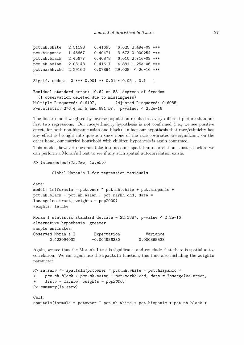
The linear model weighted by inverse population results in a very different picture than ourfirst two regressions. Our race/ethnicity hypothesis is not confirmed (i.e., we see positiveeffects for both non-hispanic asian and black). In fact our hypothesis that race/ethnicity hasany effect is brought into question since none of the race covariates are significant; on theother hand, our married household with children hypothesis is again confirmed.
This model, however does not take into account spatial autocorrelation. Just as before wecan perform a Moran’s I test to see if any such spatial autocorrelation exists.
R> lm.morantest(la.lmw, la.nbw)
Global Moran's I for regression residuals
data:
model: lm(formula = pctowner ~ pct.nh.white + pct.hispanic +
pct.nh.black + pct.nh.asian + pct.marhh.chd, data =
losangeles.tract, weights = pop2000)
weights: la.nbw
Moran I statistic standard deviate = 22.3887, p-value < 2.2e-16
alternative hypothesis: greater
sample estimates:
Observed Moran's I Expectation Variance
0.423094032 -0.004956330 0.000365538
Again, we see that the Moran’s I test is significant, and conclude that there is spatial auto-correlation. We can again use the spautolm function, this time also including the weights
parameter.
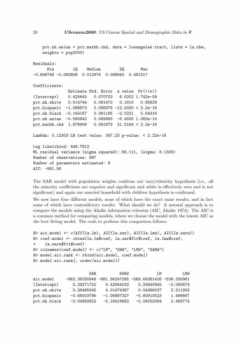
R> la.sarw <- spautolm(pctowner ~ pct.nh.white + pct.hispanic +
+ pct.nh.black + pct.nh.asian + pct.marhh.chd, data = losangeles.tract,
+ listw = la.nbw, weights = pop2000)
R> summary(la.sarw)
Call:
spautolm(formula = pctowner ~ pct.nh.white + pct.hispanic + pct.nh.black +
28 UScensus2000: US Census Spatial and Demographic Data in R
pct.nh.asian + pct.marhh.chd, data = losangeles.tract, listw = la.nbw,
weights = pop2000)
Residuals:
Min 1Q Median 3Q Max
-0.846746 -0.063808 0.012976 0.088940 0.491317
Coefficients:
Estimate Std. Error z value Pr(>|z|)
(Intercept) 0.425640 0.070702 6.0202 1.742e-09
pct.nh.white 0.014744 0.081470 0.1810 0.85639
pct.hispanic -1.068973 0.085979 -12.4330 < 2.2e-16
pct.nh.black -0.164167 0.081185 -2.0221 0.04316
pct.nh.asian -0.580842 0.089983 -6.4550 1.082e-10
pct.marhh.chd 1.976906 0.091879 21.5164 < 2.2e-16
Lambda: 0.12303 LR test value: 347.23 p-value: < 2.22e-16
Log likelihood: 448.7812
ML residual variance (sigma squared): 66.111, (sigma: 8.1309)
Number of observations: 887
Number of parameters estimated: 8
AIC: -881.56
The SAR model with population weights confirms our race/ethnicity hypothesis (i.e., allthe minority coefficients are negative and significant and white is effectively zero and is notsignificant) and again our married household with children hypothesis is confirmed.
We now have four different models, none of which have the exact same results, and in factsome of which have contradictory results. What should we do? A natural approach is tocompare the models using the Akaike information criterion (AIC, Akaike 1974). The AIC isa common method for comparing models, where we choose the model with the lowest AIC asthe best fitting model. The code to perform this comparison follows:
R> aic.model <- c(AIC(la.lm), AIC(la.sar), AIC(la.lmw), AIC(la.sarw))
R> coef.model <- cbind(la.lm$coef, la.sar$fit$coef, la.lmw$coef,
+ la.sarw$fit$coef)
R> colnames(coef.model) <- c("LM", "SAR", "LMW", "SARW")
R> model.aic.rank <- rbind(aic.model, coef.model)
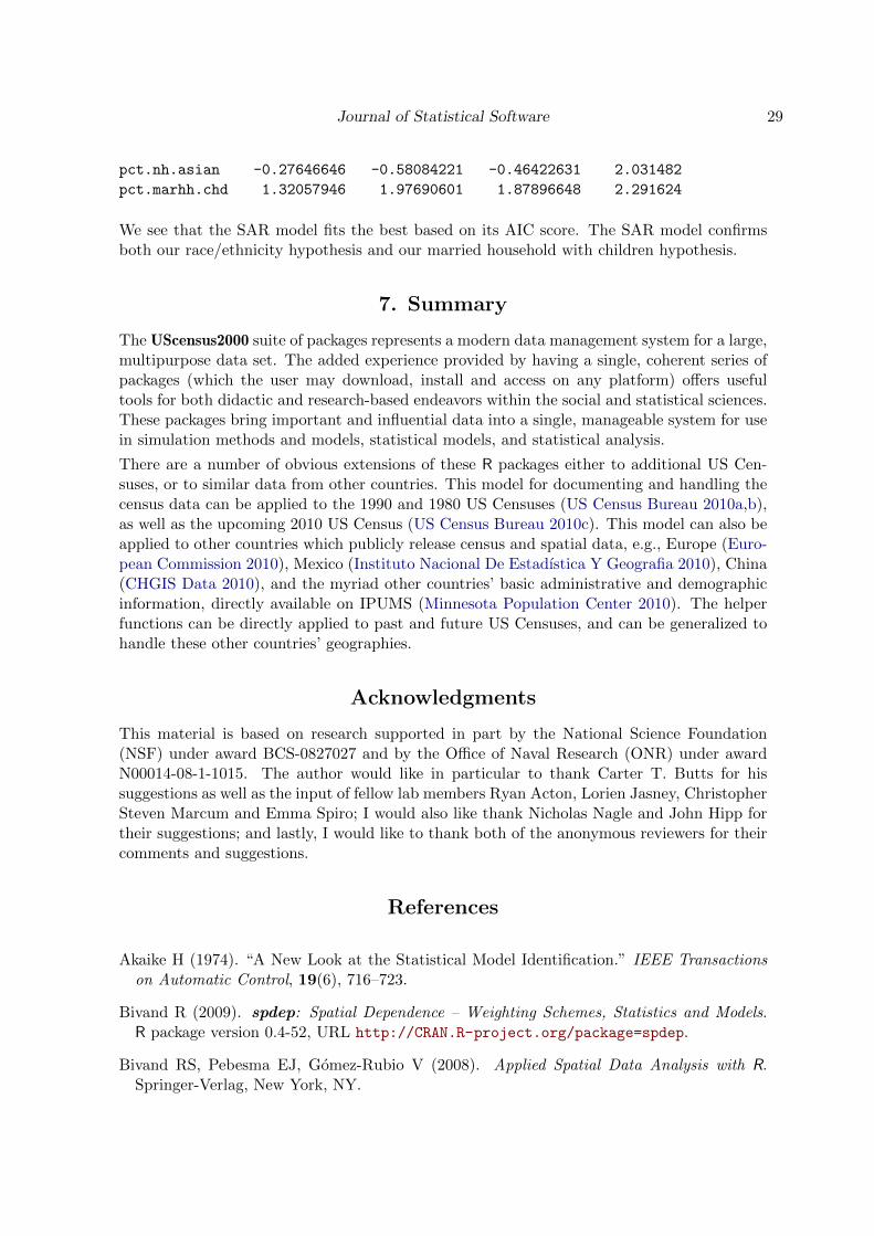
R> model.aic.rank[, order(aic.model)]
SAR SARW LM LMW
aic.model -962.36330848 -881.56247395 -569.64381426 -536.330961
(Intercept) 0.29271752 0.42564032 0.33940945 -2.093474
pct.nh.white 0.28465945 0.01474367 0.04386037 2.511933
pct.hispanic -0.65503795 -1.06897327 -0.80910523 1.486667
pct.nh.black -0.04992822 -0.16416682 -0.04052084 2.456774
Journal of Statistical Software 29
pct.nh.asian -0.27646646 -0.58084221 -0.46422631 2.031482
pct.marhh.chd 1.32057946 1.97690601 1.87896648 2.291624
We see that the SAR model fits the best based on its AIC score. The SAR model confirmsboth our race/ethnicity hypothesis and our married household with children hypothesis.
7. Summary
The UScensus2000 suite of packages represents a modern data management system for a large,multipurpose data set. The added experience provided by having a single, coherent series ofpackages (which the user may download, install and access on any platform) offers usefultools for both didactic and research-based endeavors within the social and statistical sciences.These packages bring important and influential data into a single, manageable system for usein simulation methods and models, statistical models, and statistical analysis.
There are a number of obvious extensions of these R packages either to additional US Cen-suses, or to similar data from other countries. This model for documenting and handling thecensus data can be applied to the 1990 and 1980 US Censuses (US Census Bureau 2010a,b),as well as the upcoming 2010 US Census (US Census Bureau 2010c). This model can also beapplied to other countries which publicly release census and spatial data, e.g., Europe (Euro-pean Commission 2010), Mexico (Instituto Nacional De Estadıstica Y Geografia 2010), China(CHGIS Data 2010), and the myriad other countries’ basic administrative and demographicinformation, directly available on IPUMS (Minnesota Population Center 2010). The helperfunctions can be directly applied to past and future US Censuses, and can be generalized tohandle these other countries’ geographies.
Acknowledgments
This material is based on research supported in part by the National Science Foundation(NSF) under award BCS-0827027 and by the Office of Naval Research (ONR) under awardN00014-08-1-1015. The author would like in particular to thank Carter T. Butts for hissuggestions as well as the input of fellow lab members Ryan Acton, Lorien Jasney, ChristopherSteven Marcum and Emma Spiro; I would also like thank Nicholas Nagle and John Hipp fortheir suggestions; and lastly, I would like to thank both of the anonymous reviewers for theircomments and suggestions.
References
Akaike H (1974). “A New Look at the Statistical Model Identification.” IEEE Transactionson Automatic Control, 19(6), 716–723.
Bivand R (2009). spdep: Spatial Dependence – Weighting Schemes, Statistics and Models.R package version 0.4-52, URL http://CRAN.R-project.org/package=spdep.
Bivand RS, Pebesma EJ, Gomez-Rubio V (2008). Applied Spatial Data Analysis with R.Springer-Verlag, New York, NY.
30 UScensus2000: US Census Spatial and Demographic Data in R
CHGIS Data (2010). China DCW GIS Data. Harvard University. URL http://www.fas.
harvard.edu/~chgis/data/dcw/.
European Commission (2010). Eurotat. URL http://epp.eurostat.ec.europa.eu/.
Instituto Nacional De Estadıstica Y Geografia (2010). Statistical Yearbook of the UnitedMexican States. URL http://www.inegi.org.mx/inegi/.
Keitt TH, Bivand R, Pebesma E, Rowlingson B (2009). rgdal: Bindings for the GeospatialData Abstraction Library. R package version 0.6-21, URL http://CRAN.R-project.org/
package=rgdal.
Lewin-Koh NJ, Bivand R (2009). maptools: Tools for Reading and Handling Spatial Objects.R package version 0.7-25, URL http://CRAN.R-project.org/package=maptools.
Massey DS, Denton NA (1988a). “The Dimensions of Residential Segregation.” Social Forces,67(2), 281–315.
Massey DS, Denton NA (1988b). “Suburbanization and Segregation in US MetropolitanAreas.” The American Journal of Sociology, 94(3), 592–626.
Massey DS, Denton NA (1993). American Apartheid: Segregation and the Making of theUnderclass. Harvard University Press, Cambridge.
Massey DS, Fong E (1990). “Segregation and Neighborhood Quality: Blacks, Hispanics, andAsians in the San Francisco Metropolitan Area.” Social Forces, 69(1), 15–32.
Minnesota Population Center (2010). Integrated Public Use Microdata Series, International:Version 6.0. University of Minnesota. URL https://international.ipums.org/.
Neuwirth E (2007). RColorBrewer: ColorBrewer Palettes. R package version 1.0-2, URLhttp://CRAN.R-project.org/package=RColorBrewer.
Pebesma EJ, Bivand RS (2005). “Classes and Methods for Spatial Data in R.” R News, 5(2),9–13. URL http://CRAN.R-project.org/doc/Rnews/.
Peng RD (2009). gpclib: General Polygon Clipping Library for R. R package version 1.4-4,URL http://CRAN.R-project.org/package=gpclib.
R Development Core Team (2010). R: A Language and Environment for Statistical Computing.R Foundation for Statistical Computing, Vienna, Austria. ISBN 3-900051-07-0, URL http:
//www.R-project.org/.
Temple Lang D (2009). XML: Tools for Parsing and Generating XML within R and S-PLUS.R package version 2.6-0, URL http://CRAN.R-project.org/package=XML.
US Census Bureau (2001). Census 2000 Summary File 1 United States – Prepared by the USCensus Bureau. URL http://www.census.gov/prod/cen2000/doc/sf1.pdf.
US Census Bureau (2010a). United States Census 1980. URL http://www.census.gov/
prod/www/abs/decennial/1980.htm.

Journal of Statistical Software 31
US Census Bureau (2010b). United States Census 1990. URL http://www.census.gov/
main/www/cen1990.html.
US Census Bureau (2010c). United States Census 2010. URL http://2010.census.gov/.
Worboys M, Duckham M (2004). GIS: A Computing Perspective. 2nd edition. CRC Press,Boca Raton, FL.
Affiliation:
Zack W. AlmquistDepartment of SociologyUniversity of California, Irvine3151 Social Science Plaza AIrvine, CA 92697, United States of AmericaE-mail: [email protected]: http://www.socsci.uci.edu/~almquist/
Journal of Statistical Software http://www.jstatsoft.org/
published by the American Statistical Association http://www.amstat.org/
Volume 37, Issue 6 Submitted: 2010-01-29November 2010 Accepted: 2010-10-04
Related Documents