University of Alberta - Bibliothèque et Archives Canada

University of Alberta

Power Quality Characteristics of MGN Distribution Systems

by

Janak Raj Acharya

A thesis submitted to the Faculty of Graduate Studies and Research in partial fulfillment of the requirements for the degree of

Doctor of Philosophy

in

Power Engineering and Power Electronics

Electrical and Computer Engineering

©Janak Raj Acharya Edmonton, Alberta

Fall 2010

Permission is hereby granted to the University of Alberta Libraries to reproduce single copies of this thesis and to lend or sell such copies for private, scholarly or

scientific research purposes only. Where the thesis is converted to, or otherwise made available in digital form, the University of Alberta will advise potential users of the

thesis of these terms.

The author reserves all other publication and other rights in association with the copyright in the thesis and, except as herein before provided, neither the thesis nor

any substantial portion thereof may be printed or otherwise reproduced in any material form whatsoever without the author's prior written permission.

Library and Archives Canada

Published Heritage Branch

Bibliotheque et Archives Canada

Direction du Patrimoine de I'edition

395 Wellington Street Ottawa ON K1A0N4 Canada

395, rue Wellington Ottawa ON K1A 0N4 Canada

Your file Votre reference

ISBN: 978-0-494-87885-9

Our file Notre reference

ISBN: 978-0-494-87885-9

NOTICE:

The author has granted a nonexclusive license allowing Library and Archives Canada to reproduce, publish, archive, preserve, conserve, communicate to the public by telecommunication or on the Internet, loan, distrbute and sell theses worldwide, for commercial or noncommercial purposes, in microform, paper, electronic and/or any other formats.

AVIS:

L'auteur a accorde une licence non exclusive permettant a la Bibliotheque et Archives Canada de reproduire, publier, archiver, sauvegarder, conserver, transmettre au public par telecommunication ou par I'lnternet, preter, distribuer et vendre des theses partout dans le monde, a des fins commerciales ou autres, sur support microforme, papier, electronique et/ou autres formats.

The author retains copyright ownership and moral rights in this thesis. Neither the thesis nor substantial extracts from it may be printed or otherwise reproduced without the author's permission.

L'auteur conserve la propriete du droit d'auteur et des droits moraux qui protege cette these. Ni la these ni des extraits substantiels de celle-ci ne doivent etre imprimes ou autrement reproduits sans son autorisation.

In compliance with the Canadian Privacy Act some supporting forms may have been removed from this thesis.

While these forms may be included in the document page count, their removal does not represent any loss of content from the thesis.

Conformement a la loi canadienne sur la protection de la vie privee, quelques formulaires secondaires ont ete enleves de cette these.

Bien que ces formulaires aient inclus dans la pagination, il n'y aura aucun contenu manquant.

Canada

Examining Committee

Wilsun Xu, Electrical and Computer Engineering

John Salmon, Electrical and Computer Engineering

Venkata Dinavahi, Electrical and Computer Engineering

Ming Zuo, Mechanical Engineering

David Xu, Electrical and Computer Engineering, Ryerson University

Abstract

Modern power distribution systems in North America adopt

multi-grounded neutral (MGN) configuration. The presence of the

neutral conductor and its grounding arrangement make it difficult to

understand and characterize the system's behavior. Examples are the

temporary overvoltage (TOV) and ground potential rise (GPR)

problems when the system experiences faults, and the stray voltages

and telephone interference problems when the system is in normal

operating condition.

These problems cannot be investigated by using the well-known

symmetrical-components-based techniques since they cannot include

the neutral conductors. The circuit-based simulation methods such as

the EMTP package are capable of simulating complex MGN systems,

but offer few insights into the underlying mechanisms of the electrical

phenomena involved. Therefore, some new analytical approaches that

can bridge the gaps in MGN system assessment need to be established.

The main objectives of this thesis are to develop an analytical

understanding of the electric characteristics of the MGN system, with

the phenomena of ground potential rise, temporary overvoltage and

stray voltage as the main focus. Based on the analytical results

obtained in this research, the important MGN parameters are

identified, and some of the complex phenomena are clarified. These

findings are applied to establish a novel concept that determines the

contributions of off-site and on-site sources to the stray voltage level at

the utility-customer interface point. Extensive simulation and

measurement studies demonstrate the effectiveness of the proposed

method.

Acknowledgements

First and foremost, I would like to thank and express my deep

appreciation to my supervisor, Professor Wilsun Xu, for his invaluable

guidance, support, encouragement, and patience throughout the course

of this research work. It has been my honor and privilege to work

under his supervision.

As well, I highly appreciate the scholarships, teaching assistantships,

and travel grants that I received from the University of Alberta, and

the research assistantship that I received from Professor Xu.

I would like to thank all my colleagues for their friendship and for

providing a congenial environment in the power lab. It was a great

opportunity to work with them, especially Yunfei Wang, during the

various stages of this project. I am also grateful to Dr. Ved Sharma,

Andrew Hakman and Govin Timsina for providing access to their

homes for collecting experimental data.

I am grateful to my parents and siblings in Nepal, cousin Dr. Nirmala

Sharma and her family in Saskatoon, Canada and cousin Tarapati

Paudel in Edmonton, Canada for their love, enduring support, and

encouragement.

Finally, I would like to express my sincere appreciation to my wife,

Bhagawati Poudel. Without her endless support, patience and

encouragement, this work would have never been completed. I dedicate

this thesis to her.

Table of Contents

1. Introduction 1

1.1 Problems with MGN System Performances 1

1.2 Challenges of MGN in Power System Analysis 5

1.3 Research Objectives 7

1.4 Main Contributions of the Thesis 8

1.5 Organization of the Thesis 10

1.6 Assumptions and Limitations of the Thesis 11

2. Overview of MGN Systems and Previous Research 13

2.1 Characteristics of MGN Systems 13

2.1.1 Grounding of Neutral, Substation and Transformer 14

2.1.2 Phase-to-Neutral Coupling 20

2.1.3 Load Unbalance 21

2.1.4 Neutral Current Harmonics 22

2.2 Current and Voltage Distribution in MGN Neutral 25

2.2.1 Neutral Currents and Voltages during Steady State 26

2.2.2 Neutral Currents and Voltages during Faults 27

2.3 Overview of the Previous Research 30

2.3.1 Determination of Line Parameters 30

2.3.2 Symmetrical Components and Their Limitations 33

2.3.3 Multi-phase Circuit Analysis and Tools 36

2.3.4 Secondary Circuit Analysis 39

2.4 Summary 40

3. Analytical Approaches to Ground Potential Rise Assessment 42

3.1 Ground Potential Rise of MGN Neutral 42

3.2 Proposed Approach 43

3.3 Equivalent Impedance of MGN Network 44

3.4 Mechanism of GPR Generation 49

3.4.1 Neutral Terminated in the Substation 52

3.4.2 Neutral Isolated from the Substation 53

3.4.3 Phase-to-Neutral Faults 54

3.5 Analytical and Simulation Results 55

3.6 Application Examples 57

3.6.1 Underbuilt Distribution Line 58

3.6.2 Aerial-lift Vehicle Working under the Power Lines 62

3.7 Practical Issues of Proposed Technique 64

3.7.1 Irregular Grounding Interval 64

3.7.2 Non-identical Grounding Resistances 65

3.7.3 Line-to-Line Fault 65

3.8 Conclusions 65

4. Analytical Approaches to Temporary Overvoltage Assessment....67

4.1 Introduction 67

4.2 Temporary Overvoltage Assessment 68

4.2.1 Mechanism of Temporary Overvoltage 69

4.2.2 Substation Neutral Voltage Rise 71

4.2.3 Voltage Induced by Fault Current 72

4.2.4 Voltage Induced by Neutral Current 72

4.3 Analytical and Simulation Results 77

4.4 Sensitivity Studies 79

4.4.1 Effect of Neutral Grounding Resistance 79

4.4.2 Effect of Neutral Conductor Size 80

4.4.3 Effect of Neutral Grounding Interval 81

4.5 Application of Analytical Investigations 82

4.6 Conclusions 84

5. A Novel Approach to Stray Voltage Contribution Determination. 85

5.1 Introduction 85

5.1.1 Terms and Definitions 86

5.1.2 Main Causes of Stray Voltage 88

5.2 Mechanism of Stray Voltage Generation 89

5.3 Proposed Measurement-Based Approach 90

5.3.1 Concepts and Motivation 92

5.3.2 Modeling the Stray Voltage Sources 95

5.4 Analytical Investigation 97

5.4.1 Decoupling the Neutral Current 97

5.4.2 Calculation of Current Return Ratio 99

5.4.3 Ground Currents and Their Contributions 105

5.5 Simulation Verifications 107

5.5.1 Simulation Study 107

5.5.2 Verification of Current Return Ratio 108

5.5.3 Verification of Current and Stray Voltage 109

5.6 Field Test Results Ill

5.6.1 Instrument Set-up Ill

5.6.2 Stray Voltage and Neutral Current 112

5.6.3 Neutral Current Return Ratio 113

5.6.4 Contributions of Utility and Customer 114

5.7 Application and Sensitivity Study 118

5.7.1 Customer Grounding Conditions 118

5.7.2 Secondary Neutral Conductor Conditions 119

5.7.3 Primary Neutral Grounding Conditions 121

5.7.4 Broken Primary Neutral 122

5.7.5 Operating Customer Loads Only 124

5.7.6 Operating Feeder Load Only 125

5.8 Implementation Issues 126

5.8.1 Measurement Duration 126

5.8.3 Load Configuration 130

5.9 Conclusions 133

6. Conclusions and Recommendations 135

6.1 Conclusions 135

6.2 Recommendations for Future Work 138

6.2.1 Estimating the GPR along the Neutral Length 138

6.2.2 Stray Voltage Tracking 139

References 141

Appendices 152

A. Resistance of Ground Rod with Variety of Soils 152

B. Substation Source Impedance 153

C. Stray Voltage and Neutral Current Harmonics 155

List of Tables

Table 2.1 Equivalent resistance of multiple ground rods 18

Table 3.1 MGN system impedance data 55

Table 3.2 Impedance data for the underbuilt circuit 59

Table 4.1 Nomenclature of parameters 70

Table 4.2 Phase voltage components for the fault at 6km 76

Table 4.3 Percentage contribution of individual factors to Vb 77

Table 4.4 Percentage contribution of individual factors to Vc 78

Table 5.1 Neutral network parameters 100

Table 5.2 K for various Rgn and Rc 101

Table 5.3 K for various Rgn and Rc for a bad neutral 102

Table 5.4 Customer loads and their impedance model 107

Table 5.5 Feeder loads and their impedance model 107

Table 5.6 Currents measured in the simulation 108

Table 5.7 Verification of the current return ratio (K) 109

Table 5.8 Verification of ground currents 110

Table 5.9 Comparison of the changes in currents 110

Table 5.10 Verification of stray voltages 110

Table 5.11 Stray voltages with a broken primary neutral 123

Table 5.12 Stray voltages for different loading conditions 125

Table 5.13 Impact of two-phase loads 132

Table A.l Resistivity of variety of soils and resistances of a 10ft rod. 152

List of Figures

Figure 1.1 Configurations of distribution systems 2

Figure 1.2 Four-wire MGN system 3

Figure 2.1 Layout of MGN distribution system 14

Figure 2.2 Distribution neutral grounding 15

Figure 2.3 Ground rod driven into the earth 16

Figure 2.4 Substation grid and transformer grounding 19

Figure 2.5 Distribution transformer grounding 20

Figure 2.6 Neutral current due to coupling effects 21

Figure 2.7 Many single-phase loads connected to the system 21

Figure 2.8 Currents in the three phases and neutral 22

Figure 2.9 Harmonic spectra of the currents (60Hz removed) 23

Figure 2.10 Harmonic spectra of the currents (9th to 27th order) 23

Figure 2.11 MGN system with four possible neutral layouts 25

Figure 2.12 Neutral current distribution during steady state 26

Figure 2.13 Neutral voltage distribution during steady state 27

Figure 2.14 Neutral current distribution during a fault in the middle.

28

Figure 2.15 Neutral current distribution during a fault at the end 28

Figure 2.16 Distribution of GPR during a fault in the middle 29

Figure 2.17 Distribution of GPR during a fault at the end 30

Figure 2.18 Geometry of the conductors 31

Figure 2.19 Three-phase line impedances 34

Figure 2.20 Sequence components of phase voltages 34

Figure 2.21 Analytical and simulation approaches 38

Figure 3.1 Current through a ground resistance during a fault 43

Figure 3.2 The GPR model of MGN network 44

Figure 3.3 The MGN ladder network 45

Figure 3.4 Impedance of MGN ladder for various resistances 47

Figure 3.5 Impedance of MGN ladder for various conductor sizes 47

Figure 3.6 Impedance of MGN ladder for various grounding spans. ...48

Figure 3.7 Equivalent impedance of MGN ladder at fault location 48

Figure 3.8 Induced voltages in the neutral during a SLG fault 49

Figure 3.9 Step-by-step transformation of MGN network 50

Figure 3.10 GPRs caused by the individual current sources 51

Figure 3.11 Net GPR due to two current sources 51

Figure 3.12 Shunt current sources for a line-to-wire fault 54

Figure 3.13 Distribution of GPR along the neural wire 56

Figure 3.14 Analytical and simulation results of maximum GPRs 57

Figure 3.15 Parallel transmission and distribution lines 58

Figure 3.16 Geometry of the conductors on a shared structure 59

Figure 3.17 Neutral shunt currents for a distribution line fault 60

Figure 3.18 Neutral shunt currents for a transmission line fault 61

Figure 3.19 A truck bonded to the system neutral 63

Figure 3.20 Touch voltage at truck location during a remote fault 63

Figure 4.1 Voltage rise during a fault in the adjacent phase 68

Figure 4.2 A three-phase MGN system under a SLG fault 69

Figure 4.3 Phasor representation of the TOV components 76

Figure 4.4 Main components of the temporary overvoltage 78

Figure 4.5 Comparison of analytical and simulation results 79

Figure 4.6 Effect of grounding resistance on overvoltage 80

Figure 4.7 Effect of neutral conductor size on overvoltage 81

Figure 4.8 Effect of grounding interval on overvoltage 82

Figure 4.9 TOV profiles with fault current and fault distance 83

Figure 5.1 A customer supplied from the MGN feeder 89

Figure 5.2 Electrical bonding in the service panel 90

Figure 5.3 Ground currents from the utility and customer 93

Figure 5.4 Neutral and ground current components 93

Figure 5.5 Current flow pattern in the secondary circuit 96

Figure 5.6 Equivalent model of the stray voltage sources 96

Figure 5.7 Neutral current from the customer loads only 97

Figure 5.8 Neutral current from the utility only 98

Figure 5.9 Variation of K with length of a good neutral 102

Figure 5.10 Variation of K with length of a bad neutral 103

Figure 5.11 Unbalanced current versus neutral current 104

Figure 5.12 Phasor representation of ground current components.... 105

Figure 5.13 Simulation model to verify the current return ratio 108

Figure 5.14 The measurement set-up in a residential facility Ill

Figure 5.15 Stray voltage and neutral current (Site#l) 112

Figure 5.16 Stray voltage and neutral current (Site#2) 113

Figure 5.17 The neutral current return ratio (Site #1) 113

Figure 5.18 The neutral current return ratio (Site#2) 114

Figure 5.19 Ground currents from the utility and customer (Site#l) 115

Figure 5.20 Contributions of the utility and customer (Site#l) 115

Figure 5.21 Ground currents from the utility and customer (Site#2).116

Figure 5.22 Contributions of the utility and customer (Site#2) 116

Figure 5.23 Measured SV and computed ground current (Site#l) 117

Figure 5.24 Measured SV and computed ground current (Site#2) 117

Figure 5.25 Effect of Rc on stray voltage 119

Figure 5.26 Effect of Rc on percentage contributions 119

Figure 5.27 Effect of neutral resistance on stray voltage 120

Figure 5.28 Effect of neutral resistance on percentage contribution. 120

Figure 5.29 Effect of Rgn on stray voltage 121

Figure 5.30 Effect of Rgn on percentage contributions 122

Figure 5.31 Primary neutral broken at X one at a time 123

Figure 5.32 Current flow pattern in a broken neutral 124

Figure 5.33 Percentage contributions with customer load only 125

Figure 5.34 In versus Iu for 5-min data 126



Figure 5.37 In versus Iu for 1-hour data 128

Figure 5.38 Harmonics of the neutral current 129

Figure 5.39 Harmonics of the stray voltage 129

Figure 5.40 Neutral current return ratios for the harmonics 130

Figure 5.41 Delta-wye conversion of the loads 131

Figure 5.42 Equivalent circuit with wye-connected load 131

Figure 5.43 Three-phase load supplied from the MGN system 133

Figure 6.1 The sample GPR profile 139

Figure B.l Three-phase source with impedances 153

Figure C.l Stray voltage and neutral current (60Hz) 155

Figure C.2 Stray voltage and neutral current (180Hz) 155




EMP

EMTP

GPR

IEEE

KCL

LG

LLG

MGN

MHLF

NESC

NEV

SLG

Sub

SV

TOV

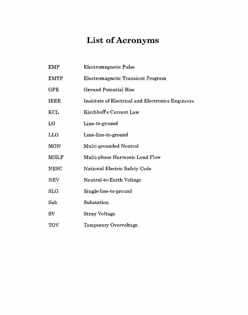
List of Acronyms

Electromagnetic Pulse

Electromagnetic Transient Program

Ground Potential Rise

Institute of Electrical and Electronics Engineers

Kirchhoff s Current Law

Line-to-ground

Line-line-to-ground

Multi-grounded Neutral

Multi-phase Harmonic Load Flow

National Electric Safety Code

Neutral-to-Earth Voltage

Single-line-to-ground

Substation

Stray Voltage

Temporary Overvoltage

1. Introduction

Modern power distribution systems are generally grounded at various

locations across the systems. According to the National Electric Safety

Code [1], the neutral conductor needs to be grounded at least four

times per mile to qualify as a multi-grounded neutral (MGN) system.

Grounding refers to the intentional connection of a system component

to the earth by means of a conductor. The objectives of grounding are to

ensure the proper operation of a system and the safety of the line

workers, public and animals. However, grounding can affect the power

system performance and power quality [2]-[4], The multi-grounding

nature of a distribution system often complicates its performance

analysis. This chapter highlights the problems associated with the

MGN system performance and discusses the challenges faced in power

system analysis concerning MGN systems. Then the objectives and

contributions of this thesis are presented. Finally, the thesis outline

and limitations of the thesis are provided.

1.1 Problems with MGN System Performances

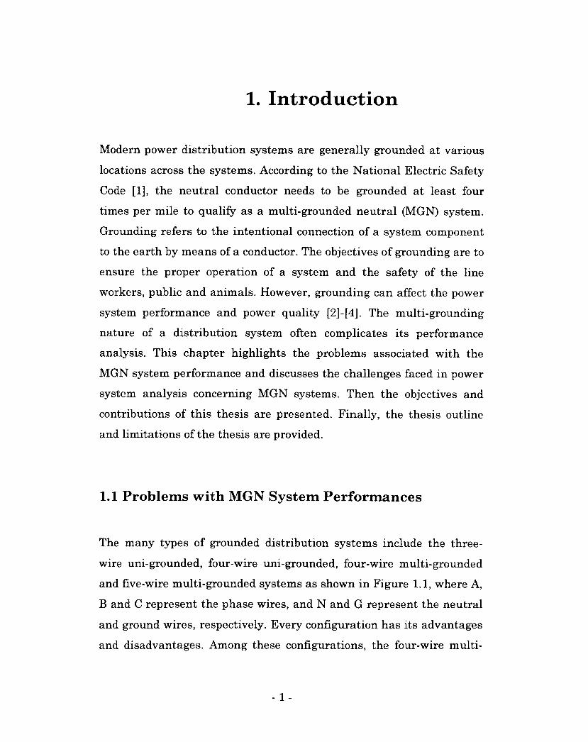
The many types of grounded distribution systems include the three-

wire uni-grounded, four-wire uni-grounded, four-wire multi-grounded

and five-wire multi-grounded systems as shown in Figure 1.1, where A,

B and C represent the phase wires, and N and G represent the neutral

and ground wires, respectively. Every configuration has its advantages

and disadvantages. Among these configurations, the four-wire multi-

- 1 -

grounded neutral (MGN) systems are the preferred choice in North

America [5]-[6]. The term "MGN system" is used throughout this thesis

to refer to the four-wire MGN systems.

(a) Three-wire uni-grounded.

N

(b) Four-wire uni-grounded.

N

TTT7T

(c) Four-wire multi-grounded.

N

T7T7T

(d) Five-wire multi-grounded.

Figure 1.1 Configurations of distribution systems.

The performance characteristics of MGN systems cause various

problems. In this thesis, the temporary overvoltage (TOV) or voltage

swell, ground potential rise (GPR) and stray voltage problems are

investigated. The TOV and GPR problems arise from the faults, or

short circuits, in the system, whereas the stray voltage problem arises

under the normal operations of the system. Historically, the GPR is

concerned mainly with the ground voltage rise in the substation. With

the advent of MGN systems, the ground voltage rise in the grounding

points of the neutral across the system has become a continuous

concern. The basic concepts associated with stray voltage, GPR and

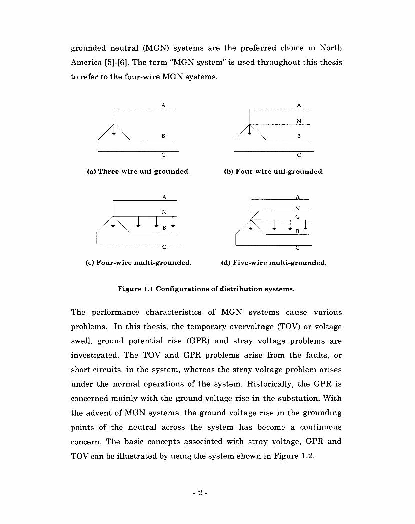
TOV can be illustrated by using the system shown in Figure 1.2.

- 2 -

Phase conductors

Aggregate loads

Source

Neutral conductor

Figure 1.2 Four-wire MGN system.

Assume that the system in Figure 1.2 is operating normally. Naturally,

the loads are not balanced. Therefore, some current will always be in

the neutral. This current also passes to the earth through the

grounding electrodes. The voltage measured between the neutral and

remote ground is called the neutral-to-earth voltage (NEV). The NEV

during the normal operation of the system is one of the main sources of

stray voltage problems because it propagates to the secondary system

through transformer neutrals. This thesis investigates the extent to

which this NEV creates stray voltage in the secondary circuit.

When this thesis was being prepared, no unanimous definition of stray

voltage existed. The most recent definition of stray voltage proposed by

the IEEE Working Group [7] is as follows:

Stray voltage refers to a voltage resulting from the normal delivery

and/or use of electricity (usually smaller than 10 volts) that may be

present between two conductive surfaces that can be

simultaneously contacted by members of the general public and/or

their animals. Stray voltage is caused by primary and/or secondary

return current, and power system induced currents, as these

- 3 -

currents flow through the impedance of the intended return

pathway, its parallel conductive pathways, and conductive loops in

close proximity to the power system.

Historically, the main concern regarding stray voltage was its

interference with dairy farm animals, but recently, stray voltage has

been a wider concern in North America. Evidence of stray voltage in

swimming pools, shower stalls, and public places has been reported [8].

As well, investigations have been carried out, and mitigation measures

have been implemented on a case-by-case basis. Contact voltage is

another phenomenon which is sometimes incorrectly referred to as

stray voltage. Contact voltage exists during faults and in levels that

can be dangerous, but is not included within the scope of this research

project.

Now consider a LG fault on Phase C between the source and loads in

Figure 1.2. Unlike the case of normal operation, a significantly large

current will flow in the neutral due to the mutual coupling effects. A

part of the neutral current dissipates to the earth through grounding

resistances, and large voltages are developed across them. The voltage

differential measured between the grounded point of the neutral and

remote earth during the system fault conditions is called the ground

potential rise (GPR). High GPR magnitudes can present a safety

hazard to the line-workers, public and animals and may also damage

nearby telecommunication cables and associated equipment.

The state of increase in the voltage magnitude above the rated

operating voltage is called temporary overvoltage (TOV) or voltage

swell. The voltage magnitude is typically between 1.1 to 1.8 times the

normal voltage for a period of up to one minute [9]-[10]. Overvoltages

- 4 -

can result in insulation failure of equipment, malfunction or damage to

equipment, or failure of surge arresters. The overvoltages in power

systems are usually generated by single-line to ground (SLG) faults,

switching off a large load, or energizing a large capacitor bank [10].

Other causes of overvoltage include a broken neutral, voltage transfer

from the high voltage side, inadvertent backfeeding of a transformer,

or ferroresonance [11]. Among these events, the SLG faults occur most

frequently. This thesis investigates the TOV associated with the SLG

faults. In the event of faults, the induction effects of the fault current

and neutral current can considerably increase the voltages of the

healthy phases.

1.2 Challenges of MGN in Power System Analysis

The MGN schemes have complications and cause problems. Multi-

grounding complicates the system design, especially in terms of

satisfying the power quality and safety requirements. Both theoretical

and technical challenges are associated with the performance analysis

of MGN systems. The symmetrical-components-based techniques used

in most power system analyses cannot be applied to the analysis of the

multi-phase systems with a multi-grounded neutral because these

techniques do not recognize the mutual coupling effects and the

neutral network. In the presence of a neutral conductor, these models

combine its impedance with the impedances of the phase conductors

and treat the grounding resistances as zero, i.e., as a solidly grounded

neutral. Other advanced techniques, such as the EMTP and load flow

programs, cannot reveal the analytical concepts of the interaction of

the various parameters. Therefore, the mechanisms or components

- 5 -

leading to the power quality and safety problems associated with MGN

systems have not been fully analyzed.

It is generally accepted that the short circuit current in MGN

distribution systems is relatively higher compared to that of other

systems. As a result, one may misunderstand that the TOV also

increases, because the traditional methods eliminate the neutral

network to simplify the problem. Similarly, the attributes of the GPR

in the MGN systems are different from those in other systems. The

highest GPR in the MGN network can be found along the neutral

conductor. However, such characteristics of MGN performance cannot

be understood unless the underlying circuit behavior is analytically

proven. This thesis presents the analytical concepts of the TOV and

GPR mechanisms in the presence of a multi-grounded neutral

conductor.

In the past, the stray voltage was found to be a problem within animal

farms, and other stray voltage issues and concerns have been well

documented in recent years. A common reason why stray voltages

originate from MGN schemes has been identified as the neutral-to-

earth voltage (NEV). The NEV transfers to the customer grounds

through the interconnection of the transformer's primary and

secondary neutrals. In addition, on-site sources such as unbalanced

loads are also responsible for stray voltages. Therefore, the

contributions of the main sources need to be identified. However, the

lack of suitable methods for such studies has been the main obstacle in

this area of research. This thesis develops a concept and investigates

the associated method for distinguishing between the main causes of

the off-site and on-site sources of the stray voltage.

- 6 -

1.3 Research Objectives

The primary objectives of the research work described in this thesis

were to investigate the MGN distribution systems to examine the

impacts of the MGN neutral on the ground potential rise (GPR),

temporary overvoltage (TOV) and stray voltage. The objectives of this

research were accomplished by focusing on the following tasks:

• Studying the mechanism of GPR generation in the MGN system

and establishing an analytical technique to determine the GPR

in the MGN neutral. The method identifies the MGN parameters

affecting the GPR.

• Investigating the potential applications of the GPR analysis

technique.

• Studying the mechanism of the TOV in MGN systems. The

neutral conductor is incorporated in the model.

• Identifying the main factors that contribute to the TOV and

developing a method to quantify these factors.

• Developing a concept and associated methods to determine the

contributions of the main stray voltage sources in the customer-

utility interface point.

• Investigating the potential applications and implementation

issues of the proposed method.

- 7 -

1.4 Main Contributions of the Thesis

In order to achieve the research objectives outlined in the previous

section, the performance of the MGN distribution system was

investigated analytically, through simulation and field tests. The main

contributions of this thesis include the following:

• This research illustrates the mechanism of GPR generation in

MGN systems. An analytical method has been developed to

evaluate the GPR. The main advantage of this method is that

the effects of main parameters, such as the grounding interval,

grounding resistance and the size of neutral conductor, can be

readily quantified.

• It is difficult to understand why the maximum GPR in the case

of MGN topology occurs along the neutral wire. A significant

finding of this work is that the maximum GPR occurs at the

location in the grounded node of the neutral where the

equivalent shunt-current source is located.

• The mechanism of the temporary overvoltage (TOV) or voltage

swell in the presence of multi-grounded neutral conductor is

studied. A 'total neutral current' approach is introduced to

incorporate the effect of the neutral currents and an analytical

tool is established to estimate the TOV. The significance of the

analytical formula is that it identifies the factors contributing to

the TOV. It is found that the neutral current can help to reduce

the TOV in the MGN systems.

- 8 -

• Another significant contribution of this thesis is the novel idea

proposed to identify the contributions of stray voltage sources at

the customer-utility interface point. The main advantage of the

proposed measurement-based technique is that the test can be

performed without switching off any loads. Moreover, the

percentage contributions are obtained by measuring the currents

only, but not the voltages so that the ground rod required for a

reference ground is also eliminated.

To date, the findings of this research have resulted in five journal

publications in the field of ground potential rise, overvoltage (or

voltage swell), and coupling effects of neutral currents [12]-[16]. The

findings of this thesis can be applied in various applications. The GPR

analysis technique can be used to estimate the GPR of any multi-

grounded conductors such as the shield wire of the transmission

system and the neutral wire of the distribution system, and the

telephone cable. The results of the TOV analysis are important in

power system applications such as the selection of surge arresters and

insulation coordination. The 'total neutral current' approach

introduced for the TOV calculation is also applicable for analyzing the

power-line-telephone interference problem and estimating the induced

voltages in nearby conductors such as pipelines and cables. The

method developed for allocating the stray voltage contributions can be

used for the trouble-shooting of a stray voltage problem by locating the

main causes. As well, this method has the potential to be implemented

into modern metering equipment to monitor the customer grounding

and neutral conditions.

- 9 -

1.5 Organization of the Thesis

This thesis is organized in six chapters as follows:

Chapter 2 provides the fundamental concepts of multi-grounded

neutral systems. Their basic characteristics such as grounding, neutral

current and voltage distributions and harmonic response are discussed.

An extensive review of previous research focusing on MGN system

performance assessment is provided. This chapter also highlights the

limitations of the existing techniques and discusses the motivation for

this present research.

Chapter 3 presents the analytical techniques for assessing the ground

potential rise (GPR) in MGN systems. The equivalent impedance

approach is introduced to simplify the problem. The GPR analysis

method identifies the factors affecting the amount of GPR that

develops during a SLG fault in the system. This method is applied to

estimate the GPR of the double-circuit line. An example of the

application of this method to the safety analysis of an aerial-lift vehicle

working under a live distribution line is also provided. The analytical

results are confirmed through simulation results.

Chapter 4 discusses the temporary overvoltage (TOV) or voltage swell

in MGN systems. The "total neutral current" approach is proposed to

incorporate the effect of neutral currents. Analytical equations are

developed, and the individual factors contributing to the TOV are

identified. The analytical results closely agree with those of the

simulation method.

- 10 -

Chapter 5 discusses the causes of stray voltage and illustrates the

mechanism of stray voltage generation. In this chapter, a

measurement-based approach is proposed for distinguishing the stray

voltage contributions of the utility (off-site source) and customer (on-

site source). The feasibility of the proposed method is verified through

analytical studies, simulations and field tests. The potential

applications of the method are investigated, and the implementation

issues such as the measurement duration and harmonics are clarified.

Chapter 6 summarizes the main conclusions of this research and

provides recommendations for the future work.

1.6 Assumptions and Limitations of the Thesis

During the preparation of this thesis, many assumptions were made to

focus on the main objectives of the project. As a result, this thesis has

some limitations including the following:

• The grounding impedance of the neutral conductor is assumed to

be purely resistive. The soil is assumed to be uniform, and its

reactance is neglected. The study of multi-layer soil structure is

beyond the scope of this thesis.

• The grounding of the substation is assumed to be resistive. The

other possible grounding configurations, such as capacitive or

inductive grounding, that may exist in the substations are

ignored.

- 11 -

• The concepts and techniques are illustrated by using the three-

phase systems only. However, except for TOV, these techniques

can be applied for single-phase systems as well.

• This project deals with the power frequency phenomena. The

effects of high frequency transients, such as lightning and

capacitive switching, are not considered in the GPR and TOV

studies.

• This research does not examine the effect of nearby electrical

installations or grounded structures on the estimated GPR of the

neutral conductor.

• The stray voltage study is limited to within the main service

panel of a customer. This study does not investigate the effects

that may have on stray voltage due to the presence of other

customers in the neighborhood.

- 12 -

2. Overview of MGN Systems and Previous Research

An overview of MGN systems is given together with a review of

previous research associated with MGN performance evaluation. First,

the characteristics of MGN systems are presented so that the problems

of MGN performance can be understood. Then developments in the

techniques and methods from the literatures are discussed by focusing

on ground potential rise, temporary overvoltage and stray voltage.

2.1 Characteristics of MGN Systems

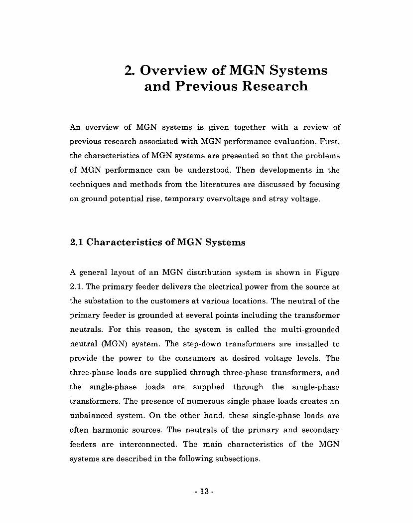
A general layout of an MGN distribution system is shown in Figure

2.1. The primary feeder delivers the electrical power from the source at

the substation to the customers at various locations. The neutral of the

primary feeder is grounded at several points including the transformer

neutrals. For this reason, the system is called the multi-grounded

neutral (MGN) system. The step-down transformers are installed to

provide the power to the consumers at desired voltage levels. The

three-phase loads are supplied through three-phase transformers, and

the single-phase loads are supplied through the single-phase

transformers. The presence of numerous single-phase loads creates an

unbalanced system. On the other hand, these single-phase loads are

often harmonic sources. The neutrals of the primary and secondary

feeders are interconnected. The main characteristics of the MGN

systems are described in the following subsections.

- 13 -

House N House 2 House 1

Secondary feeder

Single-phase transformer fy-TA

"FT

t=Hii Neutral tie

Primary feeder

i r !|[0-

Secondary feeder

Three-phase transformer

I

Secondary feeder

Single-phase transformer

Industry House 1 House 2 House N

Figure 2.1 Layout of MGN distribution system.

2.1.1 Grounding of Neutral, Substation and Transformer

Grounding refers to the intentional connection of electrical

installations to the earth by means of earth-embedded electrodes [17].

Electrical power systems are grounded for a number of reasons: (a) to

assure correct operation of electrical devices, (b) to provide safety

during normal or fault conditions, (c) to dissipate lightning strokes,

and so on. The grounding system of a typical distribution line consists

of a substation grid, neutral conductor grounding and distribution

transformer grounding.

- 14-

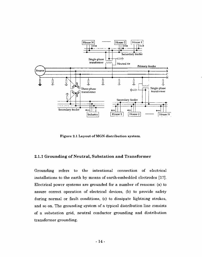
2.1.1.1 Grounding of Neutral Conductor

The neutral conductor is grounded at several locations at regular

intervals as shown in Figure 2.2. The NESC requires that the MGN

neutral be grounded at least four times per mile. The grounding is

achieved by driving a metal rod into the soil. The neutral conductor is

connected to the ground rod by means of a jumper wire capable of

carrying the maximum expected current.

Phase conductors

Neutral wire

Pole

Jumper wire

Earth surface

Ground rod

Figure 2.2 Distribution neutral grounding.

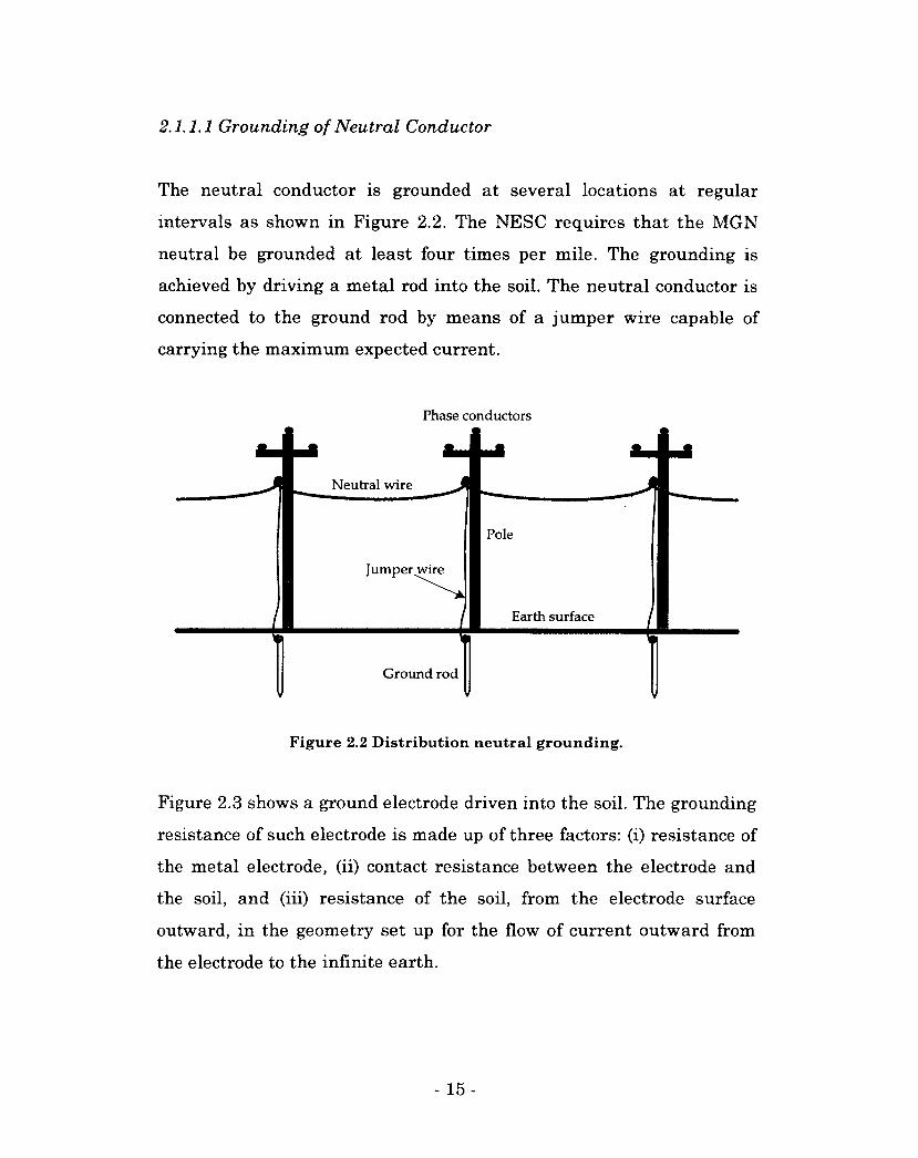
Figure 2.3 shows a ground electrode driven into the soil. The grounding

resistance of such electrode is made up of three factors: (i) resistance of

the metal electrode, (ii) contact resistance between the electrode and

the soil, and (iii) resistance of the soil, from the electrode surface

outward, in the geometry set up for the flow of current outward from

the electrode to the infinite earth.

- 15 -

Ground rod

V Earth shells

Figure 2.3 Ground rod driven into the earth.

Of the three composite factors, the soil resistance is most significant

because the first two are very small fractions of an ohm and can be

disregarded for all practical purposes. The grounding resistance is thus

determined from the resistance of the soil. The resistance around the

rod is the sum of the series resistances of virtual shells of earth,

located progressively outward from the rod. The resistance of an

element is inversely proportional to the circumferential area. The shell

nearest the rod has a small cross section, so it has the highest

resistance. Successive shells outside this one have progressively larger

cross sections or circumferential areas, and thus have progressively

lower resistances. The resistance of a ground rod is given by [18]

(2.1)

where

p = soil resistivity (Qm)

L = length of the ground rod (m)

a = radius of the ground rod (m)

n = 3.1416.

- 1 6 -

A typical ground electrode is a 10ft (3m) long and 5/8 in (16mm)

diameter rod. In practice, the diameter varies only slightly, whereas

the soil resistivity can vary from less than 10£2m to above lOOOQm.

Therefore, the rod's diameter has little effect on the grounding

resistance. The diameter is needed mainly for mechanical strength and

to ensure the rod has enough material to survive corrosion. A rod can

be driven deeper to lower the resistance when the deeper levels of the

soil have lower resistivity. If the desired resistance cannot be achieved

by using one rod, multiple ground rods in parallel can be used to

effectively reduce the overall resistance. Care must be taken when

using multiple rods. When two ground rods are too close together, they

act as one ground rod with a larger diameter, reducing much of the

gain of using parallel rods. A common rule of thumb is to separate the

rods by a distance of at least the length of one of the ground rods. The

NESC requires ground rods to be at least 6ft (1.8m) apart [18]. The

equivalent resistance of n parallel ground rods with this separation is

more than 1/n times the resistance of a single rod as given by (2.2).

Req = -xF, (2.2) n

where

R = grounding resistance of one rod

F = multiplying factor

n = number of rods in parallel.

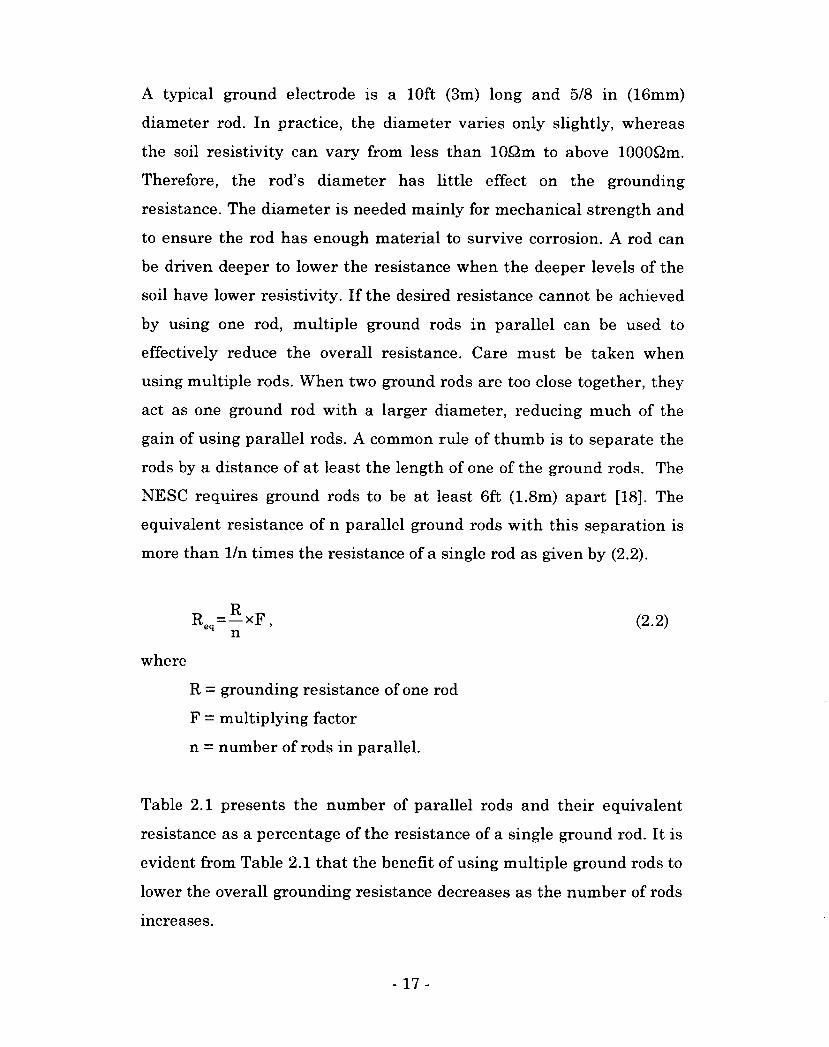
Table 2.1 presents the number of parallel rods and their equivalent

resistance as a percentage of the resistance of a single ground rod. It is

evident from Table 2.1 that the benefit of using multiple ground rods to

lower the overall grounding resistance decreases as the number of rods

increases.

- 17 -

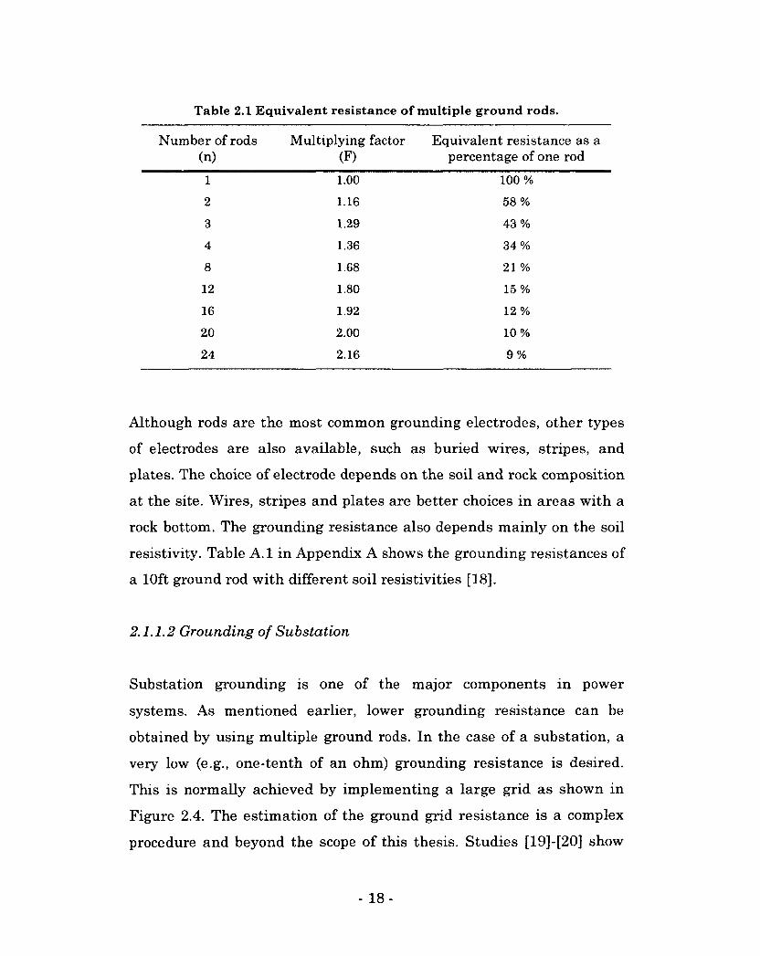
Table 2.1 Equivalent resistance of multiple ground rods.

Number of rods Multiplying factor (F)

Equivalent resistance as a percentage of one rod

1

2

3

4

8

12

16

20

24

1.00

1.16

1.29

1.36

1.68

1.80

1.92

2.00

2.16

100 %

21 %

5 8 %

4 3 %

3 4 %

15 %

12 %

10%

9%

Although rods are the most common grounding electrodes, other types

of electrodes are also available, such as buried wires, stripes, and

plates. The choice of electrode depends on the soil and rock composition

at the site. Wires, stripes and plates are better choices in areas with a

rock bottom. The grounding resistance also depends mainly on the soil

resistivity. Table A. 1 in Appendix A shows the grounding resistances of

a 10ft ground rod with different soil resistivities [18].

2.1.1.2 Grounding of Substation

Substation grounding is one of the major components in power

systems. As mentioned earlier, lower grounding resistance can be

obtained by using multiple ground rods. In the case of a substation, a

very low (e.g., one-tenth of an ohm) grounding resistance is desired.

This is normally achieved by implementing a large grid as shown in

Figure 2.4. The estimation of the ground grid resistance is a complex

procedure and beyond the scope of this thesis. Studies [19]-[20] show

- 18-

that the ground grid resistance is usually very low, e.g., less than 1Q.

In this thesis, a ground grid resistance of 0.15^2 is considered which is

typical in Alberta's substations.

Neutral

Ground wire

Ground grid

Figure 2.4 Substation grid and transformer grounding.

2.1.1.3 Grounding of Distribution Transformer

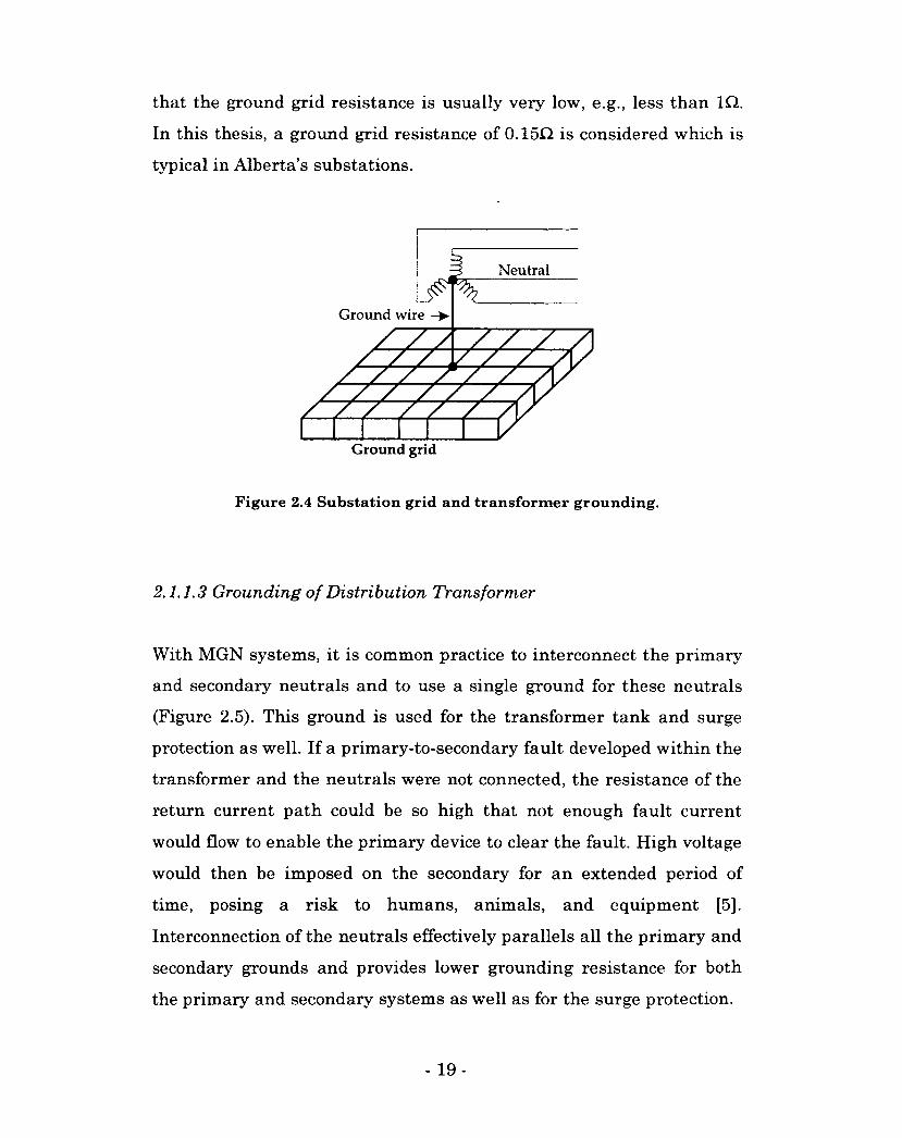
With MGN systems, it is common practice to interconnect the primary

and secondary neutrals and to use a single ground for these neutrals

(Figure 2.5). This ground is used for the transformer tank and surge

protection as well. If a primary-to-secondary fault developed within the

transformer and the neutrals were not connected, the resistance of the

return current path could be so high that not enough fault current

would flow to enable the primary device to clear the fault. High voltage

would then be imposed on the secondary for an extended period of

time, posing a risk to humans, animals, and equipment [5].

Interconnection of the neutrals effectively parallels all the primary and

secondary grounds and provides lower grounding resistance for both

the primary and secondary systems as well as for the surge protection.

- 19-

Transformer

Phase

Primary system

Arrester

Neutral Interconnection

Fhasel

Secondary

"7S5 system

Phase 2

[J Common ground

Figure 2.5 Distribution transformer grounding.

A disadvantage of this practice is the occurrence of stray voltage on the

secondary system, emanating from the high neutral-to-earth voltage

(NEV) of the primary system. The neutral of the secondary system is

bonded with the metal works such as the water pipes. This neutral

bonding is one of the main reasons for stray voltage problems in farms,

residences and swimming pools.

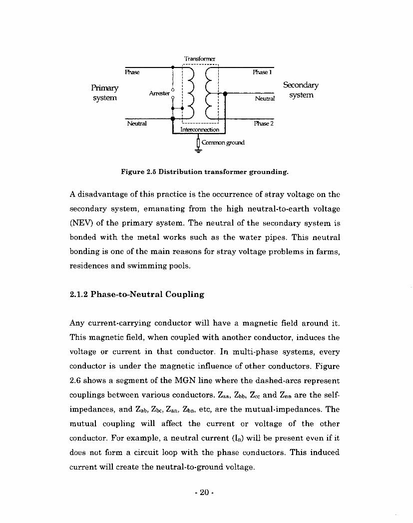
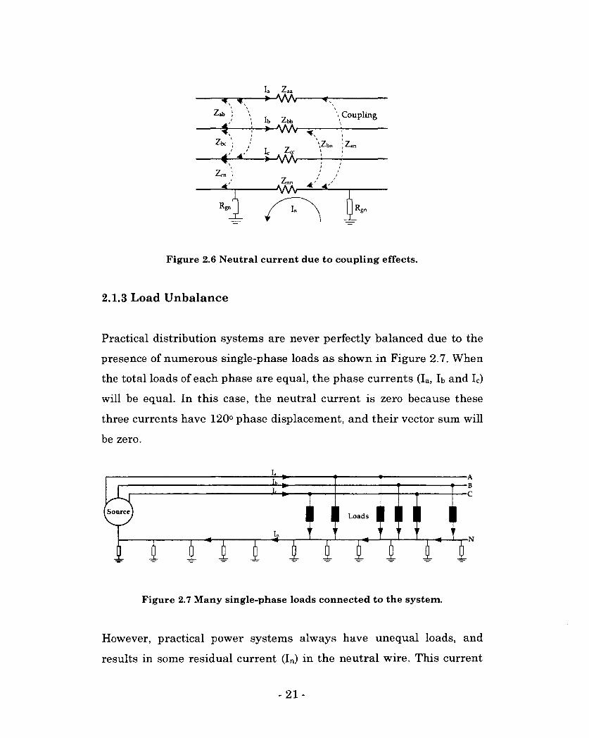
2.1.2 Phase-to-Neutral Coupling

Any current-carrying conductor will have a magnetic field around it.

This magnetic field, when coupled with another conductor, induces the

voltage or current in that conductor. In multi-phase systems, every

conductor is under the magnetic influence of other conductors. Figure

2.6 shows a segment of the MGN line where the dashed-arcs represent

couplings between various conductors. Zaa, Zbb, Zcc and Znn are the self-

impedances, and Zab, Zbc, Zan, Zbn, etc, are the mutual-impedances. The

mutual coupling will affect the current or voltage of the other

conductor. For example, a neutral current (In) will be present even if it

does not form a circuit loop with the phase conductors. This induced

current will create the neutral-to-ground voltage.

- 20-

—

Zab 1

Zbc ;

Zen I

R, gn

Ia Zaa

•MMr

lb Zbb

-^-AAAr \ Coupling

Ic Zee -*-VW-

\Zbn

Znn

•AAAr •* ̂

In

Figure 2.6 Neutral current due to coupling effects.

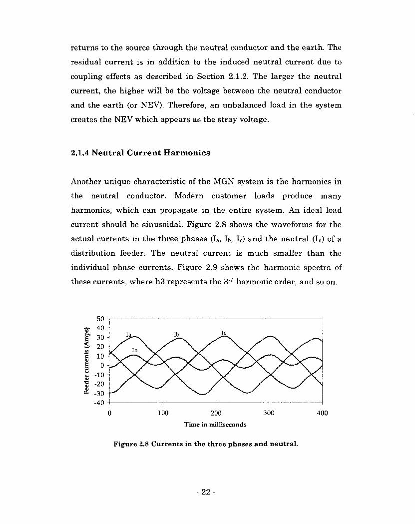
2.1.3 Load Unbalance

Practical distribution systems are never perfectly balanced due to the

presence of numerous single-phase loads as shown in Figure 2.7. When

the total loads of each phase are equal, the phase currents (Ia, lb and Ic)

will be equal. In this case, the neutral current is zero because these

three currents have 120° phase displacement, and their vector sum will

be zero.

Ih 1 LI . A I . I Source 1

Loads

I, rr i rn i i •N

Figure 2.7 Many single-phase loads connected to the system.

However, practical power systems always have unequal loads, and

results in some residual current (In) in the neutral wire. This current

- 21 -

returns to the source through the neutral conductor and the earth. The

residual current is in addition to the induced neutral current due to

coupling effects as described in Section 2.1.2. The larger the neutral

current, the higher will be the voltage between the neutral conductor

and the earth (or NEV). Therefore, an unbalanced load in the system

creates the NEV which appears as the stray voltage.

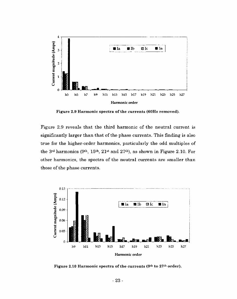
2.1.4 Neutral Current Harmonics

Another unique characteristic of the MGN system is the harmonics in

the neutral conductor. Modern customer loads produce many

harmonics, which can propagate in the entire system. An ideal load

current should be sinusoidal. Figure 2.8 shows the waveforms for the

actual currents in the three phases (Ia, lb, Ic) and the neutral (In) of a

distribution feeder. The neutral current is much smaller than the

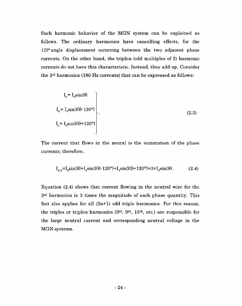
individual phase currents. Figure 2.9 shows the harmonic spectra of

these currents, where h3 represents the 3rd harmonic order, and so on.

50

01 •g -20 -01 * -30 -

-40 -

0 100 200 300 400

Time in milliseconds

Figure 2.8 Currents in the three phases and neutral.

- 22 -

4

I 3 • la H lb £3 Ic • In

01 -a

h3 h5 h7 h9 hll hl3 hl5 hl7 hl9 h21 h23 h25 h27

Harmonic order

Figure 2.9 Harmonic spectra of the currents (60Hz removed).

Figure 2.9 reveals that the third harmonic of the neutral current is

significantly larger than that of the phase currents. This finding is also

true for the higher-order harmonics, particularly the odd multiples of

the 3rd harmonics (9th, 15th, 21st and 27th), as shown in Figure 2.10. For

other harmonics, the spectra of the neutral currents are smaller than

those of the phase currents.

0.15

a g 0.12 •

• la S lb 3 Ic • In

Jj 0.09 -

i 1 0.0

£ 0.03 -3

h9 hll hl3 hi 5 hl7 hl9 h21 h23 h25 h27

Harmonic order

Figure 2.10 Harmonic spectra of the currents (9th to 27th order).

- 23 -

Such harmonic behavior of the MGN system can be explained as

follows. The ordinary harmonics have cancelling effects, for the

120° angle displacement occurring between the two adjacent phase

currents. On the other hand, the triplen (odd multiples of 3) harmonic

currents do not have this characteristic. Instead, they add up. Consider

the 3rd harmonics (180 Hz currents) that can be expressed as follows:

Ia= I3sin30

Ib=I3sin3(0-12O°) (23)

Ic= I3sin3(0+12O°)

The current that flows in the neural is the summation of the phase

currents; therefore,

In 3=I3sin30+I3sin3(e- 12O°)+I3sin3(0+12O°)=3xI3sin30. (2.4)

Equation (2.4) shows that current flowing in the neutral wire for the

3rd harmonics is 3 times the magnitude of each phase quantity. This

fact also applies for all (2n+l) odd triple harmonics. For this reason,

the triples or triplen harmonics (3rd, 9th, 15th, etc.) are responsible for

the large neutral current and corresponding neutral voltage in the

MGN systems.

- 24-

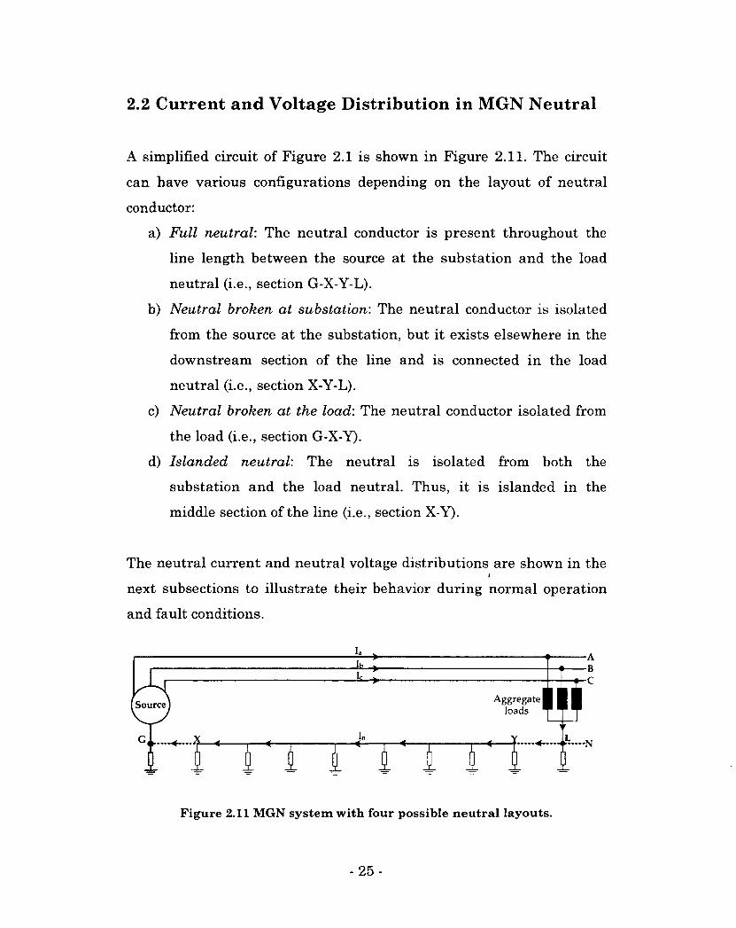
2.2 Current and Voltage Distribution in MGN Neutral

A simplified circuit of Figure 2.1 is shown in Figure 2.11. The circuit

can have various configurations depending on the layout of neutral

conductor:

a) Full neutral: The neutral conductor is present throughout the

line length between the source at the substation and the load

neutral (i.e., section G-X-Y-L).

b) Neutral broken at substation: The neutral conductor is isolated

from the source at the substation, but it exists elsewhere in the

downstream section of the line and is connected in the load

neutral (i.e., section X-Y-L).

c) Neutral broken at the load: The neutral conductor isolated from

the load (i.e., section G-X-Y).

d) Islanded neutral: The neutral is isolated from both the

substation and the load neutral. Thus, it is islanded in the

middle section of the line (i.e., section X-Y).

The neutral current and neutral voltage distributions are shown in the

next subsections to illustrate their behavior during normal operation

and fault conditions.

Source

a.

Aggregatel 11 loads T T

r l ' i ' i i ' A ' i i —< —l •N

i

Figure 2.11 MGN system with four possible neutral layouts.

- 25 -

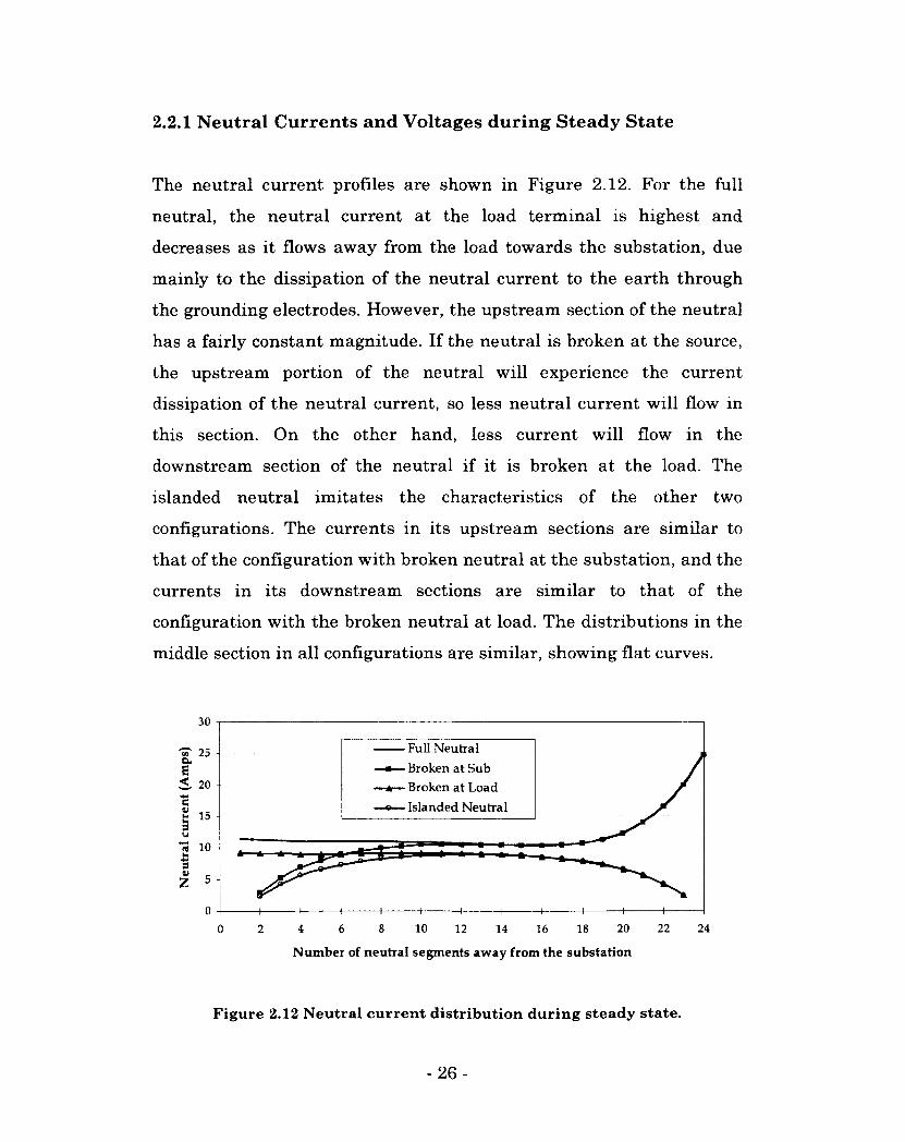
2.2.1 Neutral Currents and Voltages during Steady State

The neutral current profiles are shown in Figure 2.12. For the full

neutral, the neutral current at the load terminal is highest and

decreases as it flows away from the load towards the substation, due

mainly to the dissipation of the neutral current to the earth through

the grounding electrodes. However, the upstream section of the neutral

has a fairly constant magnitude. If the neutral is broken at the source,

the upstream portion of the neutral will experience the current

dissipation of the neutral current, so less neutral current will flow in

this section. On the other hand, less current will flow in the

downstream section of the neutral if it is broken at the load. The

islanded neutral imitates the characteristics of the other two

configurations. The currents in its upstream sections are similar to

that of the configuration with broken neutral at the substation, and the

currents in its downstream sections are similar to that of the

configuration with the broken neutral at load. The distributions in the

middle section in all configurations are similar, showing flat curves.

Full Neutral

Broken at Sub

Broken at Load

Islanded Neutral

"m 25 -

< 20

20 22 6 8 10 24 0 2 4 12 14 16 18

Number of neutral segments away from the substation

Figure 2.12 Neutral current distribution during steady state.

- 2 6 -

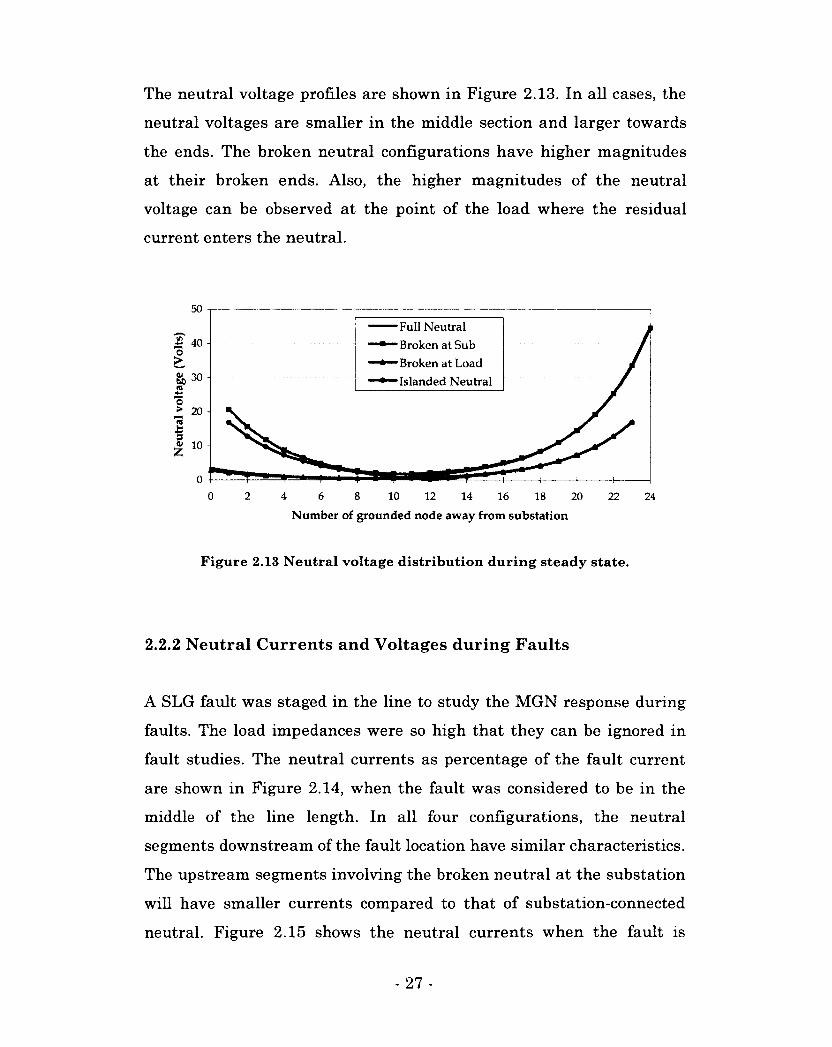
The neutral voltage profiles are shown in Figure 2.13. In all cases, the

neutral voltages are smaller in the middle section and larger towards

the ends. The broken neutral configurations have higher magnitudes

at their broken ends. Also, the higher magnitudes of the neutral

voltage can be observed at the point of the load where the residual

current enters the neutral.

Full Neutral

Broken at Sub

Broken at Load

Islanded Neutral

« 40

v 10

4 6 8 10 12 14 16 18 20

Number of grounded node away from substation

Figure 2.13 Neutral voltage distribution during steady state.

2.2.2 Neutral Currents and Voltages during Faults

A SLG fault was staged in the line to study the MGN response during

faults. The load impedances were so high that they can be ignored in

fault studies. The neutral currents as percentage of the fault current

are shown in Figure 2.14, when the fault was considered to be in the

middle of the line length. In all four configurations, the neutral

segments downstream of the fault location have similar characteristics.

The upstream segments involving the broken neutral at the substation

will have smaller currents compared to that of substation-connected

neutral. Figure 2.15 shows the neutral currents when the fault is

- 27 -

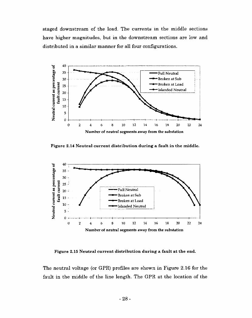
staged downstream of the load. The currents in the middle sections

have higher magnitudes, but in the downstream sections are low and

distributed in a similar manner for all four configurations.

35 - Full Neutral

Broken at Sub

Broken at Load

Islanded Neutral

30 -

10 -

12 2 8 10 14 16 18 20 22 24 0 4 6


Figure 2.14 Neutral current distribution during a fault in the middle.

35 -

30 -

Full Neutral

• Broken at Sub

* Broken at Load

• Islanded Neutral 10 -

12 8 10 14 16 18 20 22 24 0 2 4 6


Figure 2.15 Neutral current distribution during a fault at the end.

The neutral voltage (or GPR) profiles are shown in Figure 2.16 for the

fault in the middle of the line length. The GPR at the location of the

- 28-

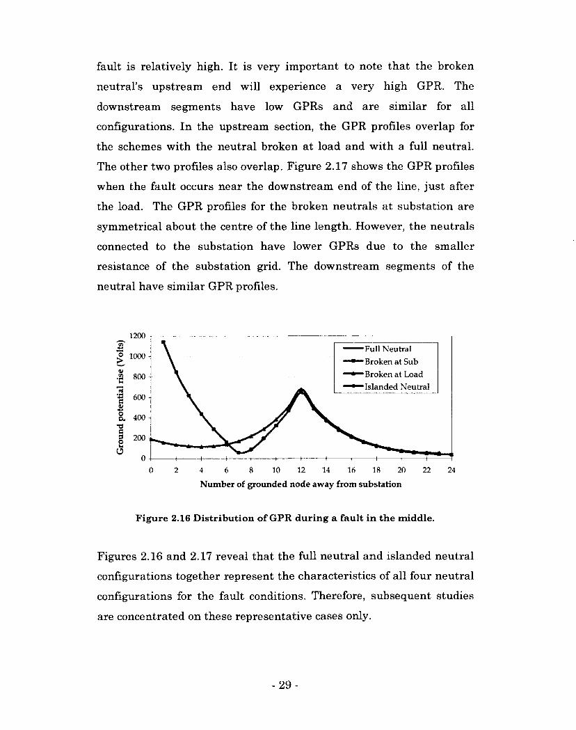
fault is relatively high. It is very important to note that the broken

neutral's upstream end will experience a very high GPR. The

downstream segments have low GPRs and are similar for all

configurations. In the upstream section, the GPR profiles overlap for

the schemes with the neutral broken at load and with a full neutral.

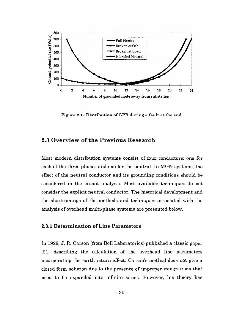
The other two profiles also overlap. Figure 2.17 shows the GPR profiles

when the fault occurs near the downstream end of the line, just after

the load. The GPR profiles for the broken neutrals at substation are

symmetrical about the centre of the line length. However, the neutrals

connected to the substation have lower GPRs due to the smaller

resistance of the substation grid. The downstream segments of the

neutral have similar GPR profiles.

1200

Full Neutral

• Broken at Sub

* Broken at Load

• Islanded Neutral

o 1000 -

12 14 18 0 2 6 8 10 16 20 22 24 4


Figure 2.16 Distribution of GPR during a fault in the middle.

Figures 2.16 and 2.17 reveal that the full neutral and islanded neutral

configurations together represent the characteristics of all four neutral

configurations for the fault conditions. Therefore, subsequent studies

are concentrated on these representative cases only.

- 29 -

800

3 700- Full Neutral

Broken at Sub

Broken at Load

Islanded Neutral

T 600 -

o 300 -a, "5 200 -

2 IOO

2 6 8 10 12 14 16 18 0 4 20 22 24


Figure 2.17 Distribution of GPR during a fault at the end.

2.3 Overview of the Previous Research

Most modern distribution systems consist of four conductors: one for

each of the three phases and one for the neutral. In MGN systems, the

effect of the neutral conductor and its grounding conditions should be

considered in the circuit analysis. Most available techniques do not

consider the explicit neutral conductor. The historical development and

the shortcomings of the methods and techniques associated with the

analysis of overhead multi-phase systems are presented below.

2.3.1 Determination of Line Parameters

In 1926, J. R. Carson (from Bell Laboratories) published a classic paper

[21] describing the calculation of the overhead line parameters

incorporating the earth return effect. Carson's method does not give a

closed form solution due to the presence of improper integrations that

need to be expanded into infinite series. However, his theory has

- 30 -

become the foundation for almost all successive methods of line

parameter calculations. The new methods are based mainly on

approximation [22].

Later, A. Deri [23] proposed the complex depth approach, which

eliminates the improper integrations of Carson's equations. In this

method, the extensive earth is replaced by a set of earth return

conductors located underneath the overhead lines with the depth of

complex value. Another advantage of this method is that additional

terms do not need to be added when calculating high-frequency

impedances. In this thesis, the line parameters were calculated using

this method, which is explained below.

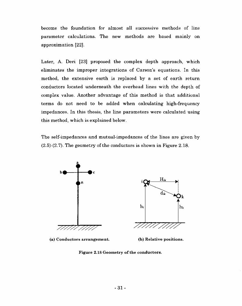
The self-impedances and mutual-impedances of the lines are given by

(2.5)-(2.7). The geometry of the conductors is shown in Figure 2.18.

»n

/////////// ///////////

(a) Conductors arrangement. (b) Relative positions.

Figure 2.18 Geometry of the conductors.

- 31 -

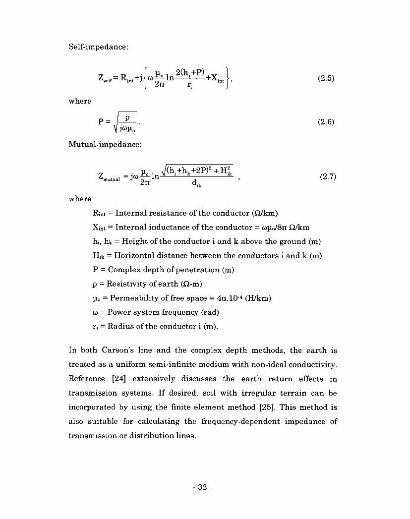
Self-impedance:

^self (2.5)

where

(2.6)

Mutual-impedance:

mutual (2.7)

where

Rint = Internal resistance of the conductor (Q/km)

Xint = Internal inductance of the conductor = «p0/8n £2/km

hi, hk = Height of the conductor i and k above the ground (m)

Hik = Horizontal distance between the conductors i and k (m)

P = Complex depth of penetration (m)

p = Resistivity of earth (£2-m)

p0 = Permeability of free space = 4n.l0 4 (H/km)

co = Power system frequency (rad)

ri = Radius of the conductor i (m).

In both Carson's line and the complex depth methods, the earth is

treated as a uniform semi-infinite medium with non-ideal conductivity.

Reference [24] extensively discusses the earth return effects in

transmission systems. If desired, soil with irregular terrain can be

incorporated by using the finite element method [25]. This method is

also suitable for calculating the frequency-dependent impedance of

transmission or distribution lines.

- 32 -

2.3.2 Symmetrical Components and Their Limitations

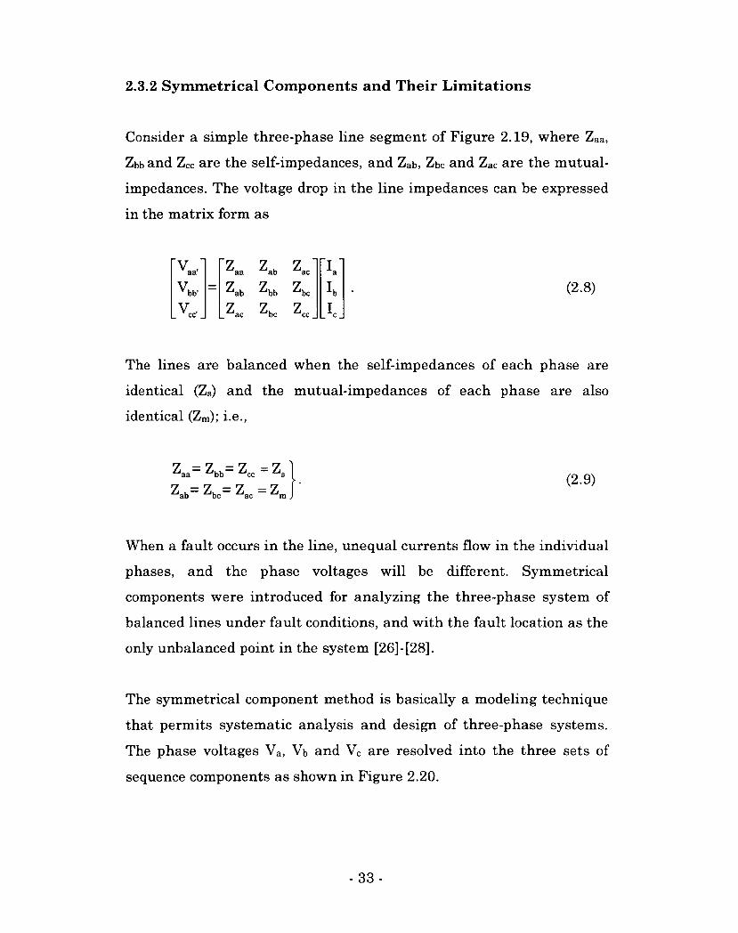
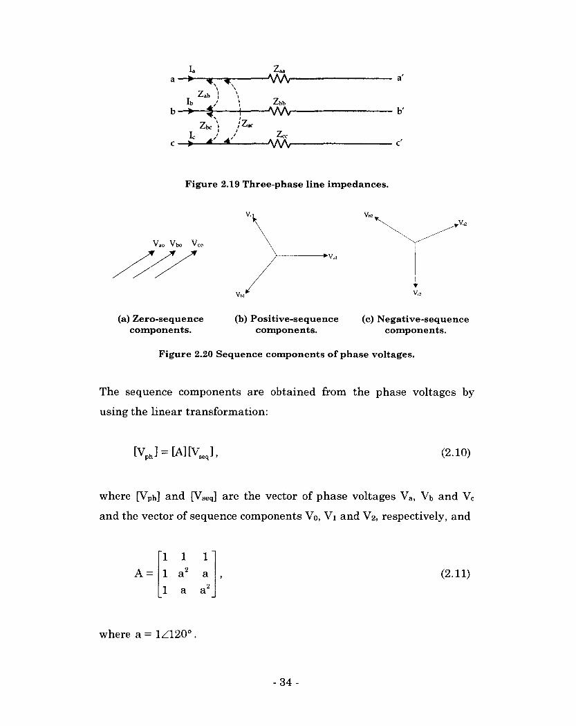
Consider a simple three-phase line segment of Figure 2.19, where Zaa,

Zbb and Zee are the self-impedances, and Zab, Zbc and Zac are the mutual-

impedances. The voltage drop in the line impedances can be expressed

in the matrix form as

Va," "Zaa Zab Zac" "la"

Vbb. r: zab Zbb Zbc lb (2.8)

Vc, .Zac Zbc Zcc Ic

The lines are balanced when the self-impedances of each phase are

identical (Zs) and the mutual-impedances of each phase are also

identical (Z m)j I.Q.,

When a fault occurs in the line, unequal currents flow in the individual

phases, and the phase voltages will be different. Symmetrical

components were introduced for analyzing the three-phase system of

balanced lines under fault conditions, and with the fault location as the

only unbalanced point in the system [26]-[28].

The symmetrical component method is basically a modeling technique

that permits systematic analysis and design of three-phase systems.

The phase voltages Va, Vb and Vc are resolved into the three sets of

sequence components as shown in Figure 2.20.

- 33 -

Ib -•

Ic

—*r Zab ! /

Zbc ) /

<7

Zaa •AAAr

Zbb -AMr b'

Zee -AAAr

Figure 2.19 Three-phase line impedances.

Vao Vbo VCI

->v»,

V*

(a) Zero-sequence components.

(b) Positive-sequence (c) Negative-sequence components. components.

Figure 2.20 Sequence components of phase voltages.

The sequence components are obtained from the phase voltages by

using the linear transformation:

[Vph] = [A][V„,], (2.10)

where [VPh] and [Vseq] are the vector of phase voltages Va, Vb and Vc

and the vector of sequence components Vo, Vi and V2, respectively, and

" 1 1 1 " A = 1 a2 a (2.11)

1 a a2

where a = 1Z1200.

- 3 4 -

Now (2.8) can be expressed as

[Vph] = [Zpl][I„J. (2.12)

By using the relationship of (2.10), Equation (2.12) becomes

tv_]= ([A]'[Zph][A])[I„„] (2.13)

[v»]=[Z„,]tI,„] (2.14)

[Z„,]=[A]'tZph][A]. (2.15)

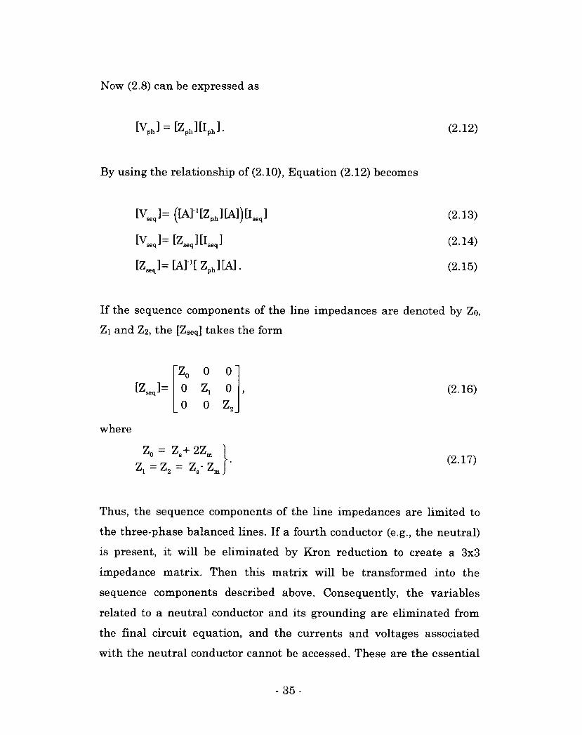
If the sequence components of the line impedances are denoted by Zo,

Zi and Z2, the [Zseq] takes the form

0

0

0

0

0

0

z,

where

Z0 = Z + 2Z_ u s m

z, = z9 = z - z 1 *-*2 s n

(2.16)

(2.17)

Thus, the sequence components of the line impedances are limited to

the three-phase balanced lines. If a fourth conductor (e.g., the neutral)

is present, it will be eliminated by Kron reduction to create a 3x3

impedance matrix. Then this matrix will be transformed into the

sequence components described above. Consequently, the variables

related to a neutral conductor and its grounding are eliminated from

the final circuit equation, and the currents and voltages associated

with the neutral conductor cannot be accessed. These are the essential

- 3 5 -

elements for the GPR, TOV and NEV analysis. Therefore, the

symmetrical components cannot represent the MGN systems. The

conventional methods that can explicitly represent the neutral

conductor and its grounding resistances are suitable.

2.3.3 Multi-phase Circuit Analysis and Tools

Historically, analytical methods were the major tools in the studies

published before powerful computers were easily accessible. In 1967, J.

Endrenyi presented an analytical method to determine the

transmission tower potentials during ground faults [29], using a multi-

grounded network. Similar grounding networks were examined for

fault current distribution in ground wires in [31]-[34], involving

exhaustive equations. In [35], Levey represented the multi-grounded

neutral by a three-terminal circuit to find the line-to-neutral fault

current for a single-phase circuit and then used this model in [36] to

compute the voltages of the multi-grounded cable. Later, in [37], he

expanded the model for a multi-phase circuit for TOV and GPR

calculations. The neutral current and GPR distribution were also

obtained by using a computer algorithm. However, these methods

failed to reveal the impact of the individual neutral parameters. In

[38], Lat presented different analytical methods to estimate the TOV in

MGN configurations, by using matrix algebra to solve the prevailing

equations for the entire system. In [39], Millard investigated the effect

of electromagnetic pulses (EMP) on the transmission line overvoltage

due to detonation of a nuclear device. Recently in 2007, an attempt to

analytically predict the overvoltage was made [40], but this study was

confined to ungrounded systems.

- 36 -

In recent years, simulation tools have been developed and become

dominant in the industry. Numerous tools and methods have been

proposed and used extensively [41]-[55]. These techniques have the

ability to represent multi-wire models and provide the opportunity to

explore the neutral current and voltages. Reference [41] discusses the

implication of using the symmetrical components in multi-phase

distribution line performance analysis. The Multi-phase Harmonic

Load Flow (MHLF) was developed in [42] to solve the harmonics and

unbalanced load flow problems. This technique also enables one to

investigate the multi-phase systems with a MGN configuration. The

neutral conductor and its multiple groundings can be explicitly

represented in the associated model. The detailed instructions are

provided in [43]. Similarly, the Electromagnetic Transient Program

(EMTP) [44] was developed to study the transients, which is

extensively used in power system transient analysis. The MHLF

technique has been integrated into the EMTP. The application of

similar multi-phase load flow techniques were examined in [45]-[46].

The effects of neutral grounding in the distribution system were

analyzed in [47]-[48] by using the EMTP approaches. The grounding

models were implemented in the EMTP to characterize the impedance

of multi-grounded neutrals on rural distribution systems in [49]-[50]

and to investigate the lightning-caused transient overvoltages in [51]-

[52]. The use of the PSpice simulation tool was proposed in [53]. While

this tool can provide the neutral currents and voltages, it cannot model

the coupling effects between the lines. Other methods, such as those in

[54]-[55], focus on improving the computational techniques.

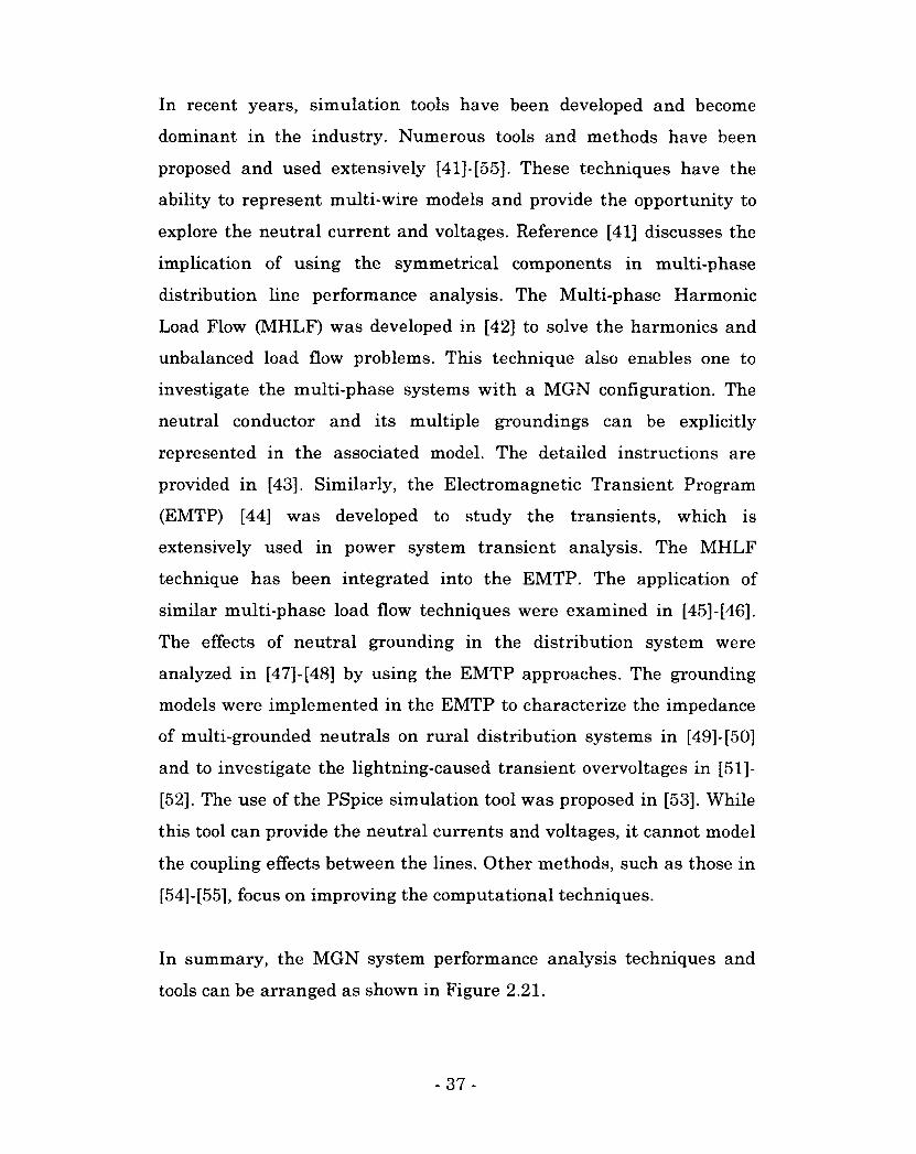
In summary, the MGN system performance analysis techniques and

tools can be arranged as shown in Figure 2.21.

- 37 -

Multi-phase Load Flow (e.g., MHLF)

EMTP (e.g., PSCAD)

Analytical approaches

Matrix algebra (e.g., Mesh equations)

Network reduction

Symmetrical components (i.e., sequence networks)

Simulation approaches

Other simulation tools (e.g., PSpice)

MGN System Performance Analysis (e.g., Overvoltage, GPR, NEV, etc.)

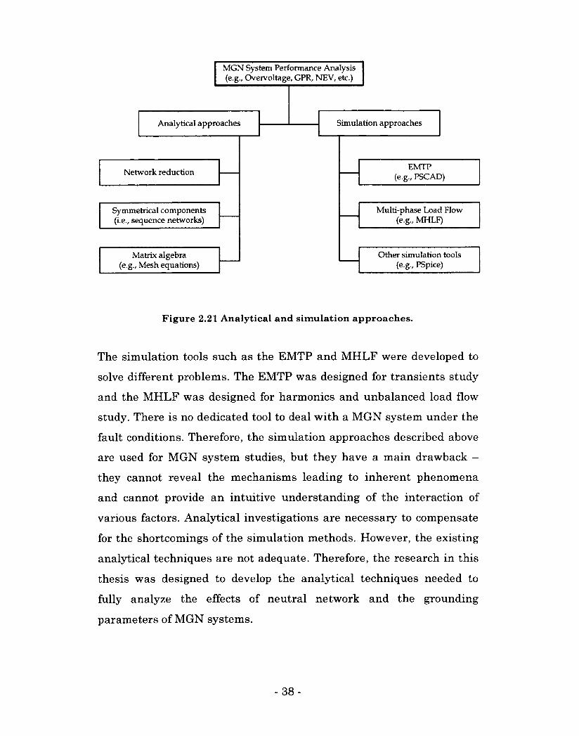
Figure 2.21 Analytical and simulation approaches.

The simulation tools such as the EMTP and MHLF were developed to

solve different problems. The EMTP was designed for transients study

and the MHLF was designed for harmonics and unbalanced load flow

study. There is no dedicated tool to deal with a MGN system under the

fault conditions. Therefore, the simulation approaches described above

are used for MGN system studies, but they have a main drawback -

they cannot reveal the mechanisms leading to inherent phenomena

and cannot provide an intuitive understanding of the interaction of

various factors. Analytical investigations are necessary to compensate

for the shortcomings of the simulation methods. However, the existing

analytical techniques are not adequate. Therefore, the research in this

thesis was designed to develop the analytical techniques needed to

fully analyze the effects of neutral network and the grounding

parameters of MGN systems.

- 3 8 -

2.3.4 Secondary Circuit Analysis

The above-mentioned methods and tools are applicable to the primary

system analysis, but they are not applicable to secondary circuit,

especially in the stray voltage assessments, because the stray voltage

on the secondary side results from both the primary and secondary

circuit conditions.

The stray voltage problems are often considered to be the side-effects of

MGN systems. The stray voltage is a small voltage, not exceeding 10V

and, thus, is not considered to be dangerous to humans [6],[8],[56]-[59].

On the other hand, cattle can be sensitive to small voltages, even IV or

less [60]-[62]. After stray voltage was initially noticed in dairy farms, it

was explored extensively by engineers and researchers wishing to

improve farm productivity [63]-[66]. The interest in stray voltage was

limited to the farm industry for many years, but in the present context,

stray voltage problems involve not only animals, but also the public.

Cases of electric shocks due to stray voltages in public facilities such as

showers and swimming pools [8] have been reported. In fact, many

jurisdictions in the US and Canada are mandating rules and

regulations in an attempt to limit stray voltage levels [67]-[68].

Experiences indicate that one of the major causes of stray voltage is

the primary neutral-to-earth voltage (NEV) resulting from four-wire

distribution systems. The four-wire MGN systems continue to remain

dominant in North America. The NEV is of concern to utilities,

regulators, and the public [71], and investigations are under way in

order to help mitigate the stray voltage problems. In [72], the NEV

originating from a nearby transmission lines by electromagnetic

- 39 -

induction was studied. The way that harmonics cause stray voltage

through an elevated NEV was discussed in [71], [73]-[76]. Other factors

affecting the NEV, such as load balancing and grounding resistances,

are presented in [77]-[78]. The primary NEV was the main focus of the

previous studies. It is well understood that stray voltage results from

both the utility system (off-site) and customer facility (on-site) [69].

Available stray voltage testing protocols [68]-[70] are based on field

measurement. Unfortunately, analytical methods for such studies are

virtually non-existent, and the question "To what extent does the

primary NEV cause stray voltage in customer facilities?" remains

unanswered analytically. Therefore, this present research was

designed to establish an analytical assessment method to quantify the

relative contributions from the off-site and on-site sources of stray

voltages.

2.4 Summary

This chapter reviewed the characteristics of MGN systems and the

progress on the techniques and methods for analyzing them. The

fundamentals of distribution system grounding, including neutral

grounding, substation grounding and transformer grounding, were

presented. Other characteristics such as coupling and neutral current

harmonics were discussed. This chapter also presented the

distributions of the voltage and current in the neutral conductor. As a

result, the representative system configurations have been identified

as the full-neutral system and islanded-neutral system.

The techniques and methods associated with the MGN system

performance evaluation available in the literature were reviewed. The

- 40 -

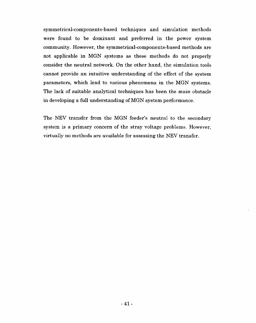
symmetrical-components-based techniques and simulation methods

were found to be dominant and preferred in the power system

community. However, the symmetrical-components-based methods are

not applicable in MGN systems as these methods do not properly

consider the neutral network. On the other hand, the simulation tools

cannot provide an intuitive understanding of the effect of the system

parameters, which lead to various phenomena in the MGN systems.

The lack of suitable analytical techniques has been the main obstacle

in developing a full understanding of MGN system performance.

The NEV transfer from the MGN feeder's neutral to the secondary

system is a primary concern of the stray voltage problems. However,

virtually no methods are available for assessing the NEV transfer.

- 41 -

3. Analytical Approaches to Ground Potential Rise

Assessment

An analytical model for ground potential rise (GPR) assessment is

proposed. Analytical studies of the GPR phenomena associated with

MGN configurations are conducted. This chapter also reveals the

mechanisms leading to the phenomena and their affecting factors.

Approximate formulae are derived to quantify the impacts of various

factors. Simulation is performed to compare its results with the

analytical results. The effects of different parameters associated with

the MGN neutral are presented through sensitivity studies. The

application of proposed technique is demonstrated by using examples

of underbuilt distribution system and the aerial-lift vehicle working

under live power lines.

3.1 Ground Potential Rise of MGN Neutral

Consider a system like that represented in Figure 3.1 where a LG fault

in a MGN feeder drives a large amount of current in the phase wire,

the neutral wire, and the substation grounding resistance. The neutral

current dissipates into the earth through the grounding resistances,

leading to a large GPR in each grounded node of the neutral. The GPR

of any grounded node is the voltage potential of that node measured

with respect to the remote earth.

- 42 -

Aggregate loads

•A B C

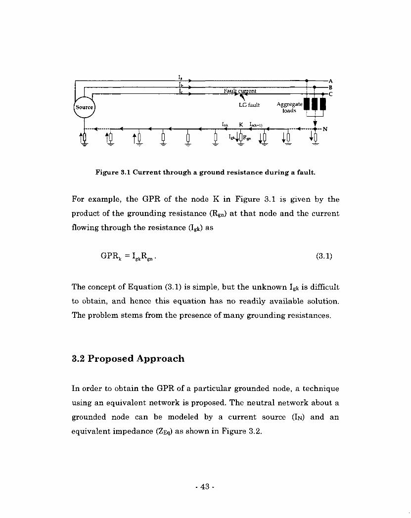
Figure 3.1 Current through a ground resistance during a fault.

For example, the GPR of the node K in Figure 3.1 is given by the

product of the grounding resistance (Rgn) at that node and the current

flowing through the resistance (Igk) as

The concept of Equation (3.1) is simple, but the unknown Igk is difficult

to obtain, and hence this equation has no readily available solution.

The problem stems from the presence of many grounding resistances.

3.2 Proposed Approach

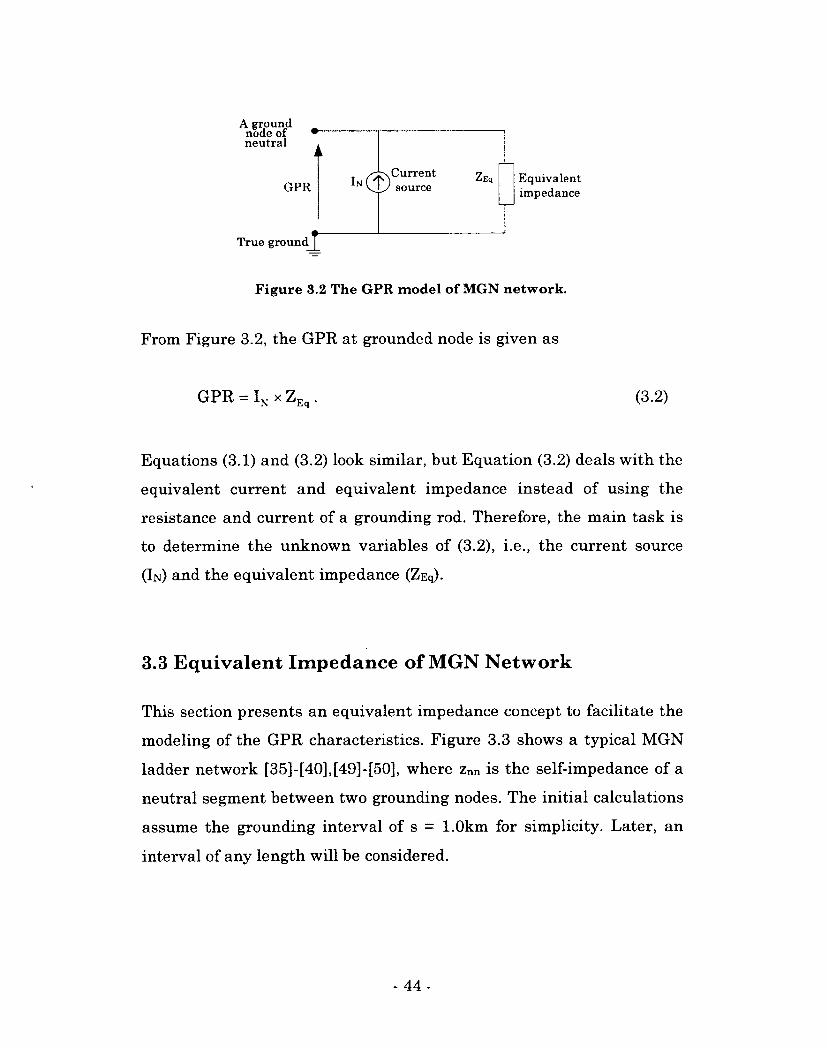
In order to obtain the GPR of a particular grounded node, a technique

using an equivalent network is proposed. The neutral network about a

grounded node can be modeled by a current source (IN) and an

equivalent impedance (ZEq) as shown in Figure 3.2.

GPRk Igk^gn • (3.1)

- 43 -

A ground node of • neutral

A

GPR

True ground

Current source

ZEq Equivalent impedance

Figure 3.2 The GPR model of MGN network.

From Figure 3.2, the GPR at grounded node is given as

GPR = IN x ZEq . (3.2)

Equations (3.1) and (3.2) look similar, but Equation (3.2) deals with the

equivalent current and equivalent impedance instead of using the

resistance and current of a grounding rod. Therefore, the main task is

to determine the unknown variables of (3.2), i.e., the current source

(In) and the equivalent impedance (zeq).

3.3 Equivalent Impedance of MGN Network

This section presents an equivalent impedance concept to facilitate the

modeling of the GPR characteristics. Figure 3.3 shows a typical MGN

ladder network [35]-[40],[49]-[50], where znn is the self-impedance of a

neutral segment between two grounding nodes. The initial calculations

assume the grounding interval of s = 1.0km for simplicity. Later, an

interval of any length will be considered.

- 44 -

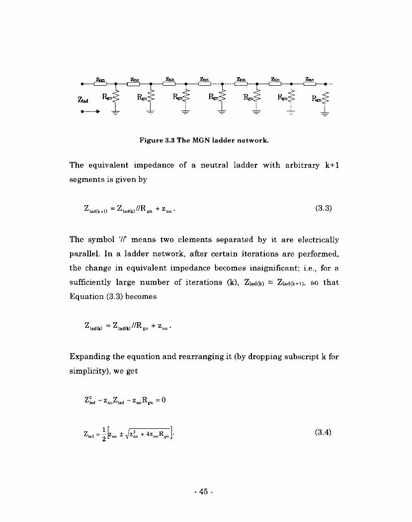
Zlnd Rgn^> Rgn^> Rgn<I R™

— ± -L ± I 1 1 ±

Figure 3.3 The MGN ladder network.

The equivalent impedance of a neutral ladder with arbitrary k+1

segments is given by

The symbol 'IT means two elements separated by it are electrically

parallel. In a ladder network, after certain iterations are performed,

the change in equivalent impedance becomes insignificant; i.e., for a

sufficiently large number of iterations (k), Ziad(k) ~ Ziad(k+i>, so that

Equation (3.3) becomes

^ lad(k) ~~ ^ lad(k) gn ^nn '

Expanding the equation and rearranging it (by dropping subscript k for

simplicity), we get

Z lad(k+l) lad(k) (3.3)

^lad Znn^lad Znn^gn ~~ ^

(3.4)

-45-

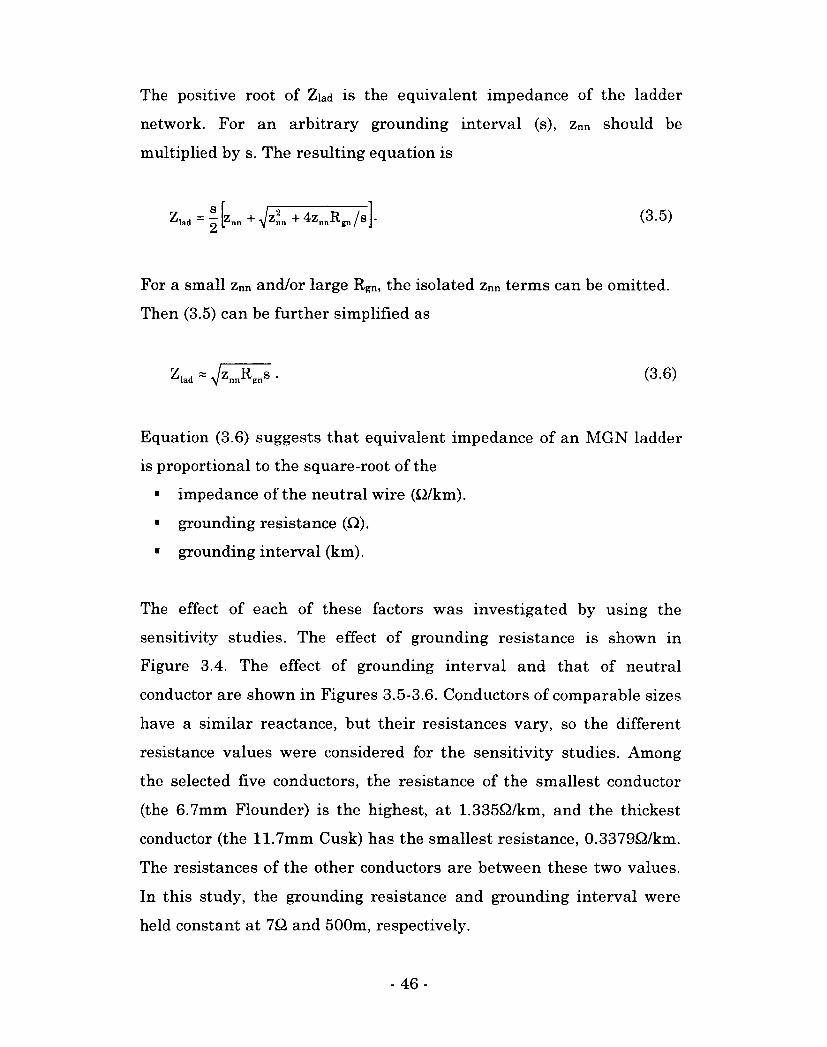
The positive root of Ziad is the equivalent impedance of the ladder

network. For an arbitrary grounding interval (s), znn should be

multiplied by s. The resulting equation is

For a small znn and/or large Rgn, the isolated znn terms can be omitted.

Then (3.5) can be further simplified as

Equation (3.6) suggests that equivalent impedance of an MGN ladder

is proportional to the square-root of the

• impedance of the neutral wire (Q/km).

• grounding resistance (Q).

• grounding interval (km).

The effect of each of these factors was investigated by using the

sensitivity studies. The effect of grounding resistance is shown in

Figure 3.4. The effect of grounding interval and that of neutral

conductor are shown in Figures 3.5-3.6. Conductors of comparable sizes

have a similar reactance, but their resistances vary, so the different

resistance values were considered for the sensitivity studies. Among

the selected five conductors, the resistance of the smallest conductor

(the 6.7mm Flounder) is the highest, at 1.335£2/km, and the thickest

conductor (the 11.7mm Cusk) has the smallest resistance, 0.3379Q/km.

The resistances of the other conductors are between these two values.

In this study, the grounding resistance and grounding interval were

held constant at 70, and 500m, respectively.

(3.5)

(3.6)

- 46 -

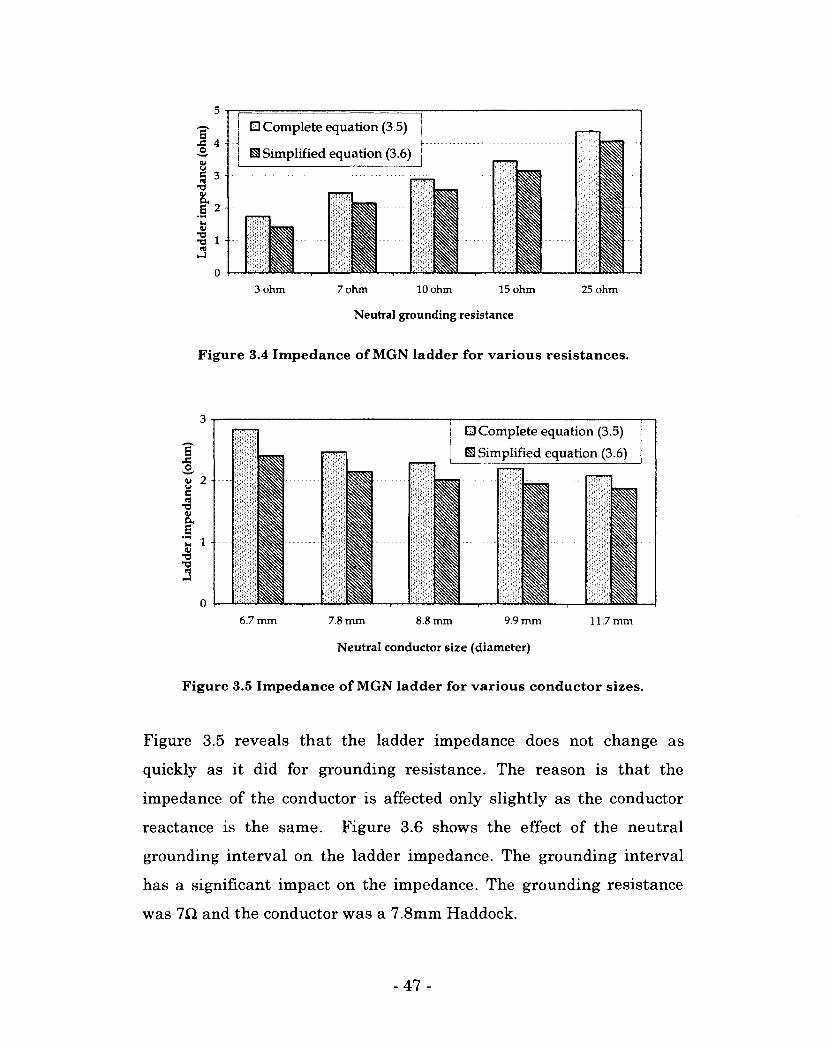
ED Complete equation (3.5)

• Simplified equation (3.6)

3 ohm 7 ohm 10 ohm 15 ohm 25 ohm

Neutral grounding resistance

Figure 3.4 Impedance of MGN ladder for various resistances.

GO Complete equation (3.5)

El Simplified equation (3.6)

6.7 mm 7.8 nun 8.8 mm 9.9 mm

Neutral conductor size (diameter)

11.7 mm

Figure 3.5 Impedance of MGN ladder for various conductor sizes.

Figure 3.5 reveals that the ladder impedance does not change as

quickly as it did for grounding resistance. The reason is that the

impedance of the conductor is affected only slightly as the conductor

reactance is the same. Figure 3.6 shows the effect of the neutral

grounding interval on the ladder impedance. The grounding interval

has a significant impact on the impedance. The grounding resistance

was 7Q and the conductor was a 7.8mm Haddock.

-47 -

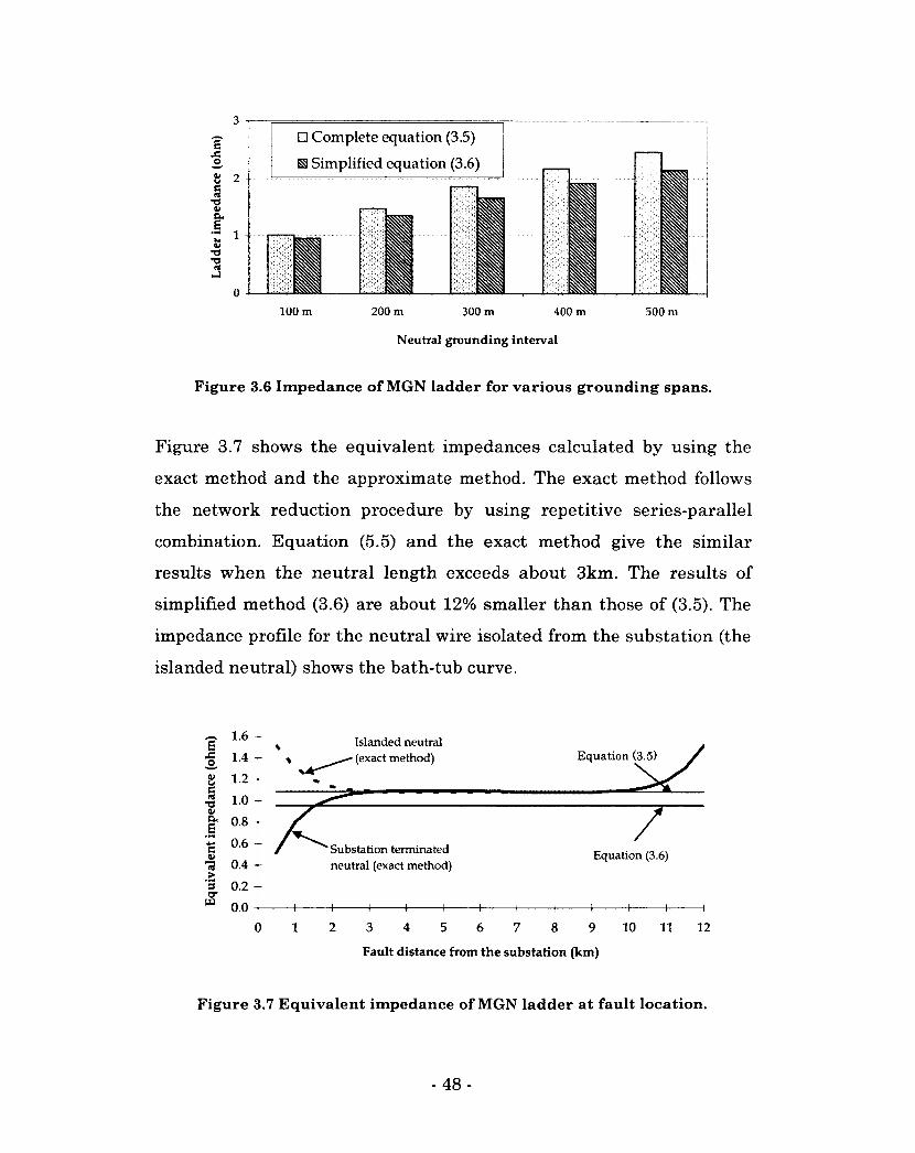
s

V o u z C <« T3 4> a s <u

T3 H3 nJ

1 -

• Complete equation (3.5)

^ Simplified equation (3.6)

100 m 200 m 300 m 400 m

Neutral grounding interval

500 m

Figure 3.6 Impedance of MGN ladder for various grounding spans.

Figure 3.7 shows the equivalent impedances calculated by using the

exact method and the approximate method. The exact method follows

the network reduction procedure by using repetitive series-parallel

combination. Equation (5.5) and the exact method give the similar

results when the neutral length exceeds about 3km. The results of

simplified method (3.6) are about 12% smaller than those of (3.5). The

impedance profile for the neutral wire isolated from the substation (the

islanded neutral) shows the bath-tub curve.

0.8 --

0.6 -

Islanded neutral (exact method)

Substation terminated neutral (exact method)

-+- -4-

Equation (3. (3.5) /

/ Equation (3.6)

-+-

3 4 5 6 7 8 9

Fault distance from the substation (km)

10 11 12

Figure 3.7 Equivalent impedance of MGN ladder at fault location.

- 48 -

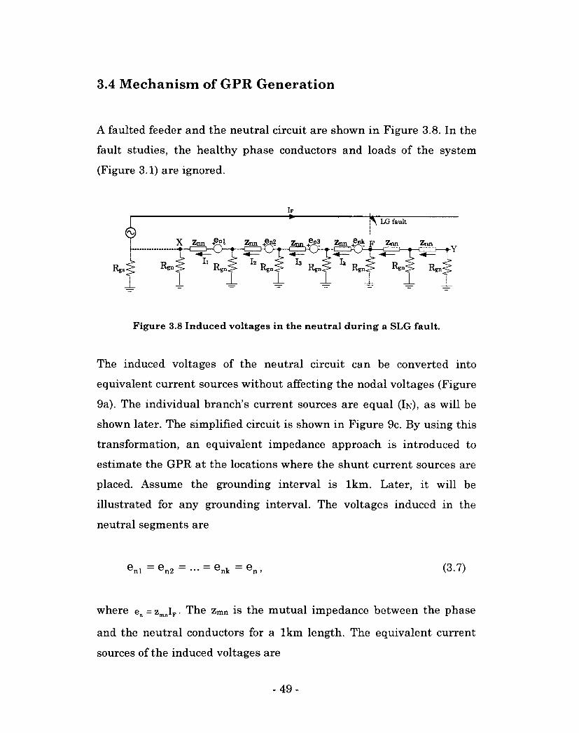
3.4 Mechanism of GPR Generation

A faulted feeder and the neutral circuit are shown in Figure 3.8. In the

fault studies, the healthy phase conductors and loads of the system

(Figure 3.1) are ignored.

IF

Figure 3.8 Induced voltages in the neutral during a SLG fault.

The induced voltages of the neutral circuit can be converted into

equivalent current sources without affecting the nodal voltages (Figure

9a). The individual branch's current sources are equal (IN), as will be

shown later. The simplified circuit is shown in Figure 9c. By using this

transformation, an equivalent impedance approach is introduced to

estimate the GPR at the locations where the shunt current sources are

placed. Assume the grounding interval is 1km. Later, it will be

illustrated for any grounding interval. The voltages induced in the

neutral segments are

enl = en2 = = enk = en > (3.7)

where en = zmnIF • The zmn is the mutual impedance between the phase

and the neutral conductors for a 1km length. The equivalent current

sources of the induced voltages are

-49-

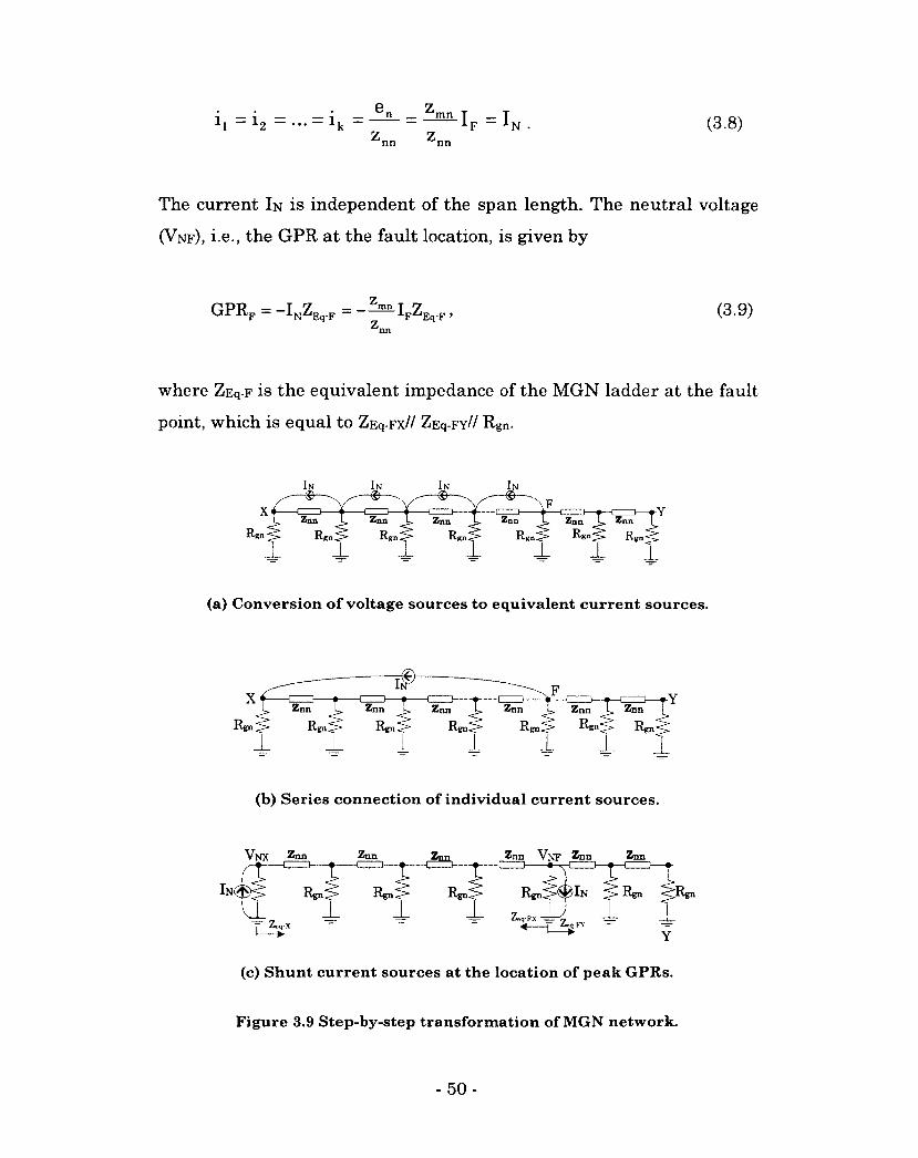
ij = i2 = ... = ik = = -âs-Ip = IN . (3.8) Znn Znn

The current IN is independent of the span length. The neutral voltage

(VNF), i.e., the GPR at the fault location, is given by

GPRF = -INZEqF = -^MFZEq.F, (3.9) Z nn

where ZEq-F is the equivalent impedance of the MGN ladder at the fault

point, which is equal to ZEq-Fx// Zeq-fy// Rgn.

Znn Znn Znn Znn Znn Znn

'gn; •gn

(a) Conversion of voltage sources to equivalent current sources.

•—i 1 > Znn Znn Znn Znn Znn

Rgn

(b) Series connection of individual current sources.

(c) Shunt current sources at the location of peak GPRs.

Figure 3.9 Step-by-step transformation of MGN network.

- 50 -

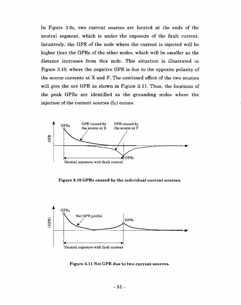
In Figure 3.9c, two current sources are located at the ends of the

neutral segment, which is under the exposure of the fault current.

Intuitively, the GPR of the node where the current is injected will be

higher than the GPRs of the other nodes, which will be smaller as the

distance increases from this node. This situation is illustrated in

Figure 3.10, where the negative GPR is due to the opposite polarity of

the source currents at X and F. The combined effect of the two sources

will give the net GPR as shown in Figure 3.11. Thus, the locations of

the peak GPRs are identified as the grounding nodes where the

injection of the current sources (IN) occurs.

GPR caused by GPR caused by the source at X the source at F

GPRx

•

Neutral exposure with fault current

Figure 3.10 GPRs caused by the individual current sources.

GPRx

Net GPR profile GPRF

Neutral exposure with fault current

Figure 3.11 Net GPR due to two current sources.

- 51 -

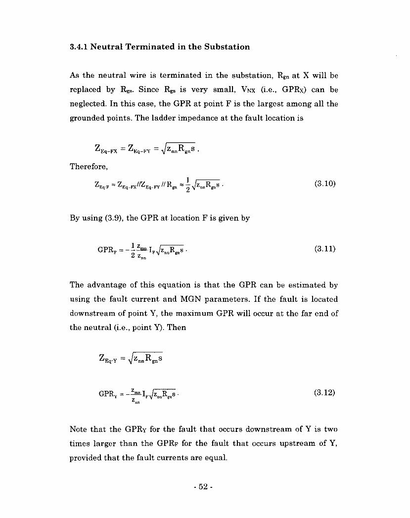
3.4.1 Neutral Terminated in the Substation

As the neutral wire is terminated in the substation, Rgn at X will be

replaced by Rgs. Since Rgs is very small, VNX (i.e., GPRx) can be

neglected. In this case, the GPR at point F is the largest among all the

grounded points. The ladder impedance at the fault location is

Êq-FX — Êq-FY — V2nn^gnS •

Therefore,

(3'10)

By using (3.9), the GPR at location F is given by

GPRF = -I^BBLI Jz R a • (3.11) » n „ f V nn gn

nn

The advantage of this equation is that the GPR can be estimated by

using the fault current and MGN parameters. If the fault is located

downstream of point Y, the maximum GPR will occur at the far end of

the neutral (i.e., point Y). Then

Êq-Y = -y/ZnnRgnS

GPRY=-?mIF^J^J. (3.12) z nn

Note that the GPRY for the fault that occurs downstream of Y is two

times larger than the GPRF for the fault that occurs upstream of Y,

provided that the fault currents are equal.

- 52 -

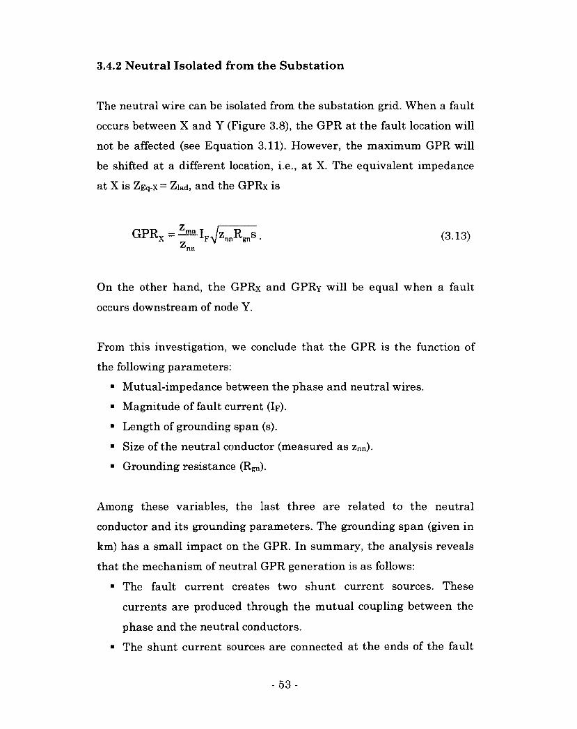
3.4.2 Neutral Isolated from the Substation

The neutral wire can be isolated from the substation grid. When a fault

occurs between X and Y (Figure 3.8), the GPR at the fault location will

not be affected (see Equation 3.11). However, the maximum GPR will

be shifted at a different location, i.e., at X. The equivalent impedance

at X is ZEq-x = Ziad, and the GPRx is

On the other hand, the GPRx and GPRY will be equal when a fault

occurs downstream of node Y.

From this investigation, we conclude that the GPR is the function of

the following parameters:

• Mutual-impedance between the phase and neutral wires.

• Magnitude of fault current (IF).

• Length of grounding span (s).

• Size of the neutral conductor (measured as znn).

• Grounding resistance (Rgn).

Among these variables, the last three are related to the neutral

conductor and its grounding parameters. The grounding span (given in

km) has a small impact on the GPR. In summary, the analysis reveals

that the mechanism of neutral GPR generation is as follows:

• The fault current creates two shunt current sources. These

currents are produced through the mutual coupling between the

phase and the neutral conductors.

• The shunt current sources are connected at the ends of the fault

(3.13)

- 53 -

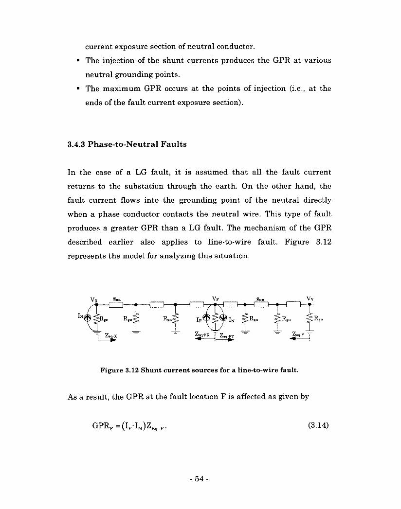
current exposure section of neutral conductor.

• The injection of the shunt currents produces the GPR at various

neutral grounding points.

• The maximum GPR occurs at the points of injection (i.e., at the

ends of the fault current exposure section).

3.4.3 Phase-to-Neutral Faults

In the case of a LG fault, it is assumed that all the fault current

returns to the substation through the earth. On the other hand, the

fault current flows into the grounding point of the neutral directly

when a phase conductor contacts the neutral wire. This type of fault

produces a greater GPR than a LG fault. The mechanism of the GPR

described earlier also applies to line-to-wire fault. Figure 3.12

represents the model for analyzing this situation.

As a result, the GPR at the fault location F is affected as given by

Figure 3.12 Shunt current sources for a line-to-wire fault.

GPRF - (iF^NÊq-F • (3.14)

- 54 -

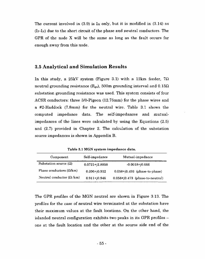
The current involved in (3.9) is IN only, but it is modified in (3.14) as

(IF-IN) due to the short circuit of the phase and neutral conductors. The

GPR of the node X will be the same as long as the fault occurs far

enough away from this node.

3.5 Analytical and Simulation Results

In this study, a 25kV system (Figure 3.1) with a 12km feeder, 7Q

neutral grounding resistance (Rgn), 500m grounding interval and 0.15H

substation grounding resistance was used. This system consists of four

ACSR conductors: three 3/0-Pigeon (12.75mm) for the phase wires and

a #2-Haddock (7.8mm) for the neutral wire. Table 3.1 shows the

computed impedance data. The self-impedances and mutual-

impedances of the lines were calculated by using the Equations (2.5)

and (2.7) provided in Chapter 2. The calculation of the substation

source impedances is shown in Appendix B.

Table 3.1 MGN system impedance data.

Component Self-impedance Mutual-impedance

Substation source (Q) 0.0721+j2.8858 -0.0018+j0.666

Phase conductors (Q/km) 0.396+j0.912 0.058+j0.493 (phase-to-phase)

Neutral conductor (ft /km) 0.911+jO.946 0.058+j0.473 (phase-to-neutral)

The GPR profiles of the MGN neutral are shown in Figure 3.13. The

profiles for the case of neutral wire terminated at the substation have

their maximum values at the fault locations. On the other hand, the

islanded neutral configuration exhibits two peaks in its GPR profiles -

one at the fault location and the other at the source side end of the

- 55-

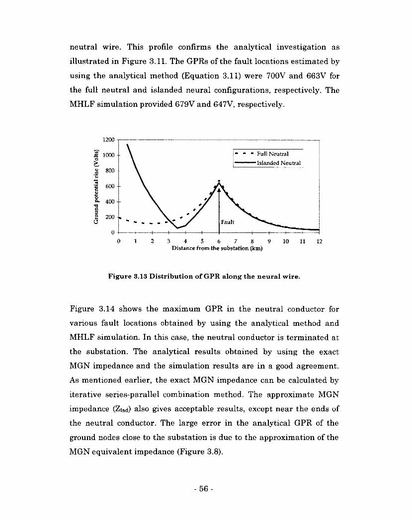
neutral wire. This profile confirms the analytical investigation as

illustrated in Figure 3.11. The GPRs of the fault locations estimated by

using the analytical method (Equation 3.11) were 700V and 663V for

the full neutral and islanded neural configurations, respectively. The

MHLF simulation provided 679V and 647V, respectively.

1200

Full Neutral

Islanded Neutral 1000 --

600 --

a- 400

200 Fault

0 1 2 3 4 5 6 7 8 9 10 12 11 Distance from the substation (km)

Figure 3.13 Distribution of GPR along the neural wire.

Figure 3.14 shows the maximum GPR in the neutral conductor for

various fault locations obtained by using the analytical method and

MHLF simulation. In this case, the neutral conductor is terminated at

the substation. The analytical results obtained by using the exact

MGN impedance and the simulation results are in a good agreement.

As mentioned earlier, the exact MGN impedance can be calculated by

iterative series-parallel combination method. The approximate MGN

impedance (Ziad) also gives acceptable results, except near the ends of

the neutral conductor. The large error in the analytical GPR of the

ground nodes close to the substation is due to the approximation of the

MGN equivalent impedance (Figure 3.8).

- 56 -

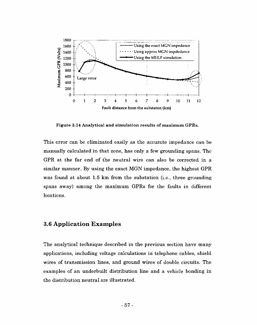
1800 ~i—

1600 •• / Using the exact MGN impedance

Using approx MGN impdedance

Using; the MHLF simulation

* 1400 --

1200

1000 --U g 800 -

I 600 --

J 400 -S

200 --

0 -0 1 2 3 4 5 6 7 8 9 1 0 1 1 1 2

Fault distance from the substaton (km)

Figure 3.14 Analytical and simulation results of maximum GPRs.

This error can be eliminated easily as the accurate impedance can be

manually calculated in that zone, has only a few grounding spans. The

GPR at the far end of the neutral wire can also be corrected in a

similar manner. By using the exact MGN impedance, the highest GPR

was found at about 1.5 km from the substation (i.e., three grounding

spans away) among the maximum GPRs for the faults in different

locations.

3.6 Application Examples

The analytical technique described in the previous section have many

applications, including voltage calculations in telephone cables, shield

wires of transmission lines, and ground wires of double circuits. The

examples of an underbuilt distribution line and a vehicle bonding in

the distribution neutral are illustrated.

- 57 -

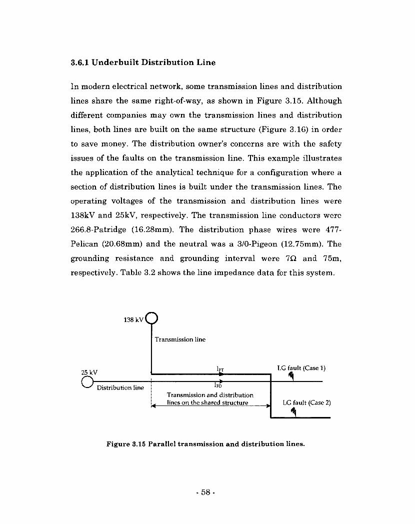
3.6.1 Underbuilt Distribution Line

In modern electrical network, some transmission lines and distribution

lines share the same right-of-way, as shown in Figure 3.15. Although

different companies may own the transmission lines and distribution

lines, both lines are built on the same structure (Figure 3.16) in order

to save money. The distribution owner's concerns are with the safety

issues of the faults on the transmission line. This example illustrates

the application of the analytical technique for a configuration where a

section of distribution lines is built under the transmission lines. The

operating voltages of the transmission and distribution lines were

138kV and 25kV, respectively. The transmission line conductors were

266.8-Patridge (16.28mm). The distribution phase wires were 477-

Pelican (20.68mm) and the neutral was a 3/0-Pigeon (12.75mm). The

grounding resistance and grounding interval were 7Q. and 75m,

respectively. Table 3.2 shows the line impedance data for this system.

Transmission line

25 kV I FT LG fault (Case 1)

i o Distribution line Transmission and distribution lines on the shared structure LG fault (Case 2)

Figure 3.15 Parallel transmission and distribution lines.

- 58 -

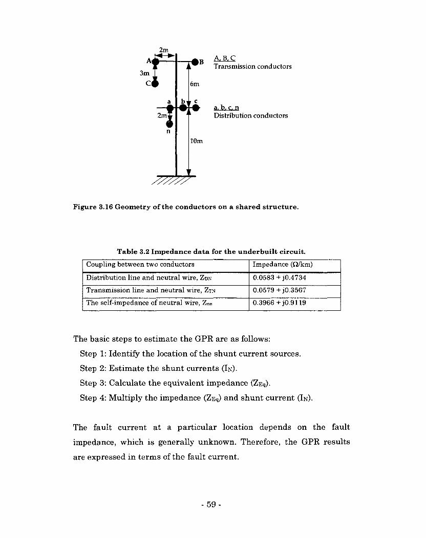
2m Ai

3m

C

f i*B

i

2m.

10m

A. B.C Transmission conductors

a, b, c. n Distribution conductors

Figure 3.16 Geometry of the conductors on a shared structure.

Table 3.2 Impedance data for the underbuilt circuit.

Coupling between two conductors Impedance (T2/km)

Distribution line and neutral wire, ZDN 0.0583 + j0.4734

Transmission line and neutral wire, ZTN 0.0579+j0.3567

The self-impedance of neutral wire, Znn 0.3966+j0.9119

The basic steps to estimate the GPR are as follows:

Step 1: Identify the location of the shunt current sources.

Step 2: Estimate the shunt currents (IN).

Step 3: Calculate the equivalent impedance (ZEq).

Step 4: Multiply the impedance (ZEq) and shunt current (IN).

The fault current at a particular location depends on the fault

impedance, which is generally unknown. Therefore, the GPR results

are expressed in terms of the fault current.

- 59 -

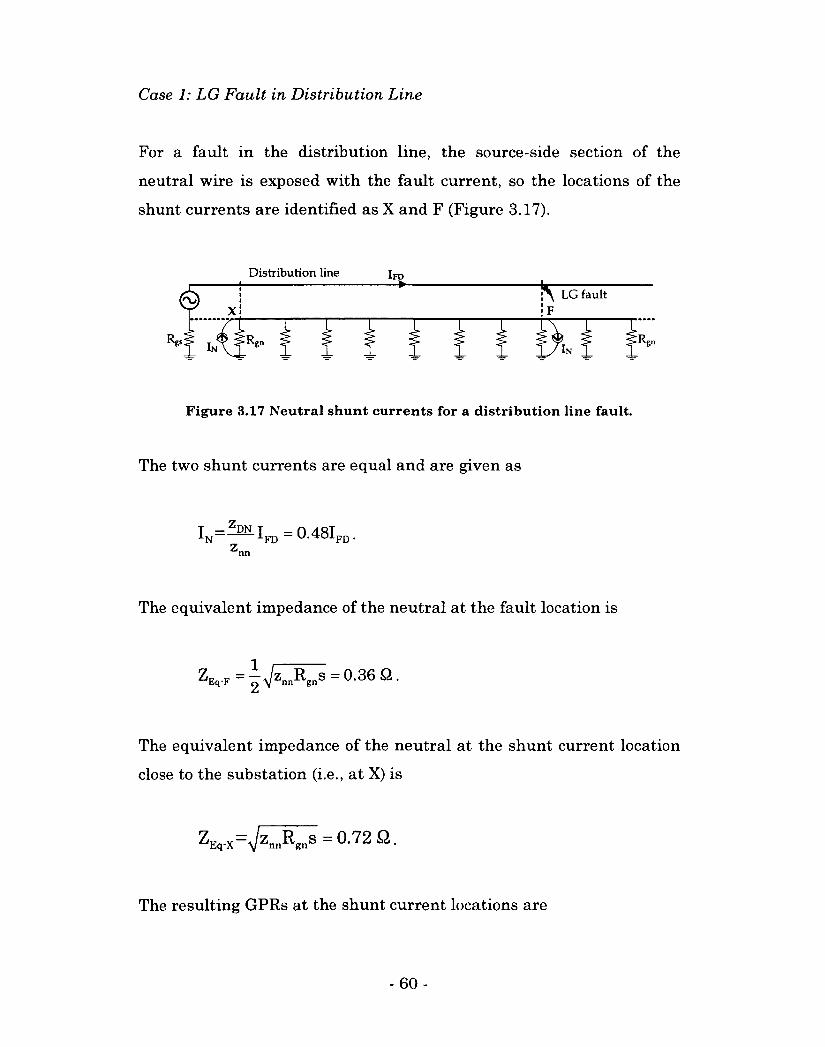
Case 1: LG Fault in Distribution Line

For a fault in the distribution line, the source-side section of the

neutral wire is exposed with the fault current, so the locations of the

shunt currents are identified as X and F (Figure 3.17).

Distribution line Ipp

Figure 3.17 Neutral shunt currents for a distribution line fault.

The two shunt currents are equal and are given as

IN=SALIRO=0.48IPD. Znn

The equivalent impedance of the neutral at the fault location is

ZF„.F = -JznnRras = 0.36 Q. "Q * 2 * g

The equivalent impedance of the neutral at the shunt current location

close to the substation (i.e., at X) is

ZFnX=\/Zm,R<mS = 0-72 Q . bq-A yj nn gn

The resulting GPRs at the shunt current locations are

-60-

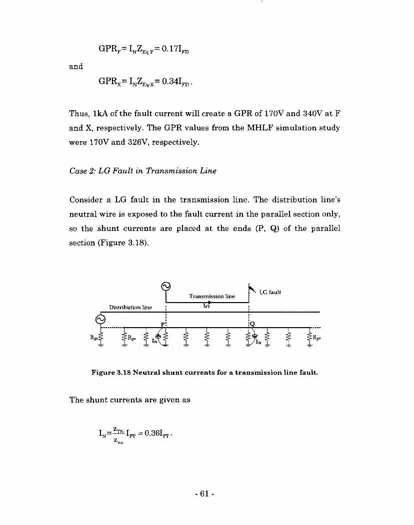
GPRF- lAqF- 0.17IFD

and

GPRX= INZEqX= 0.34Ifd

Thus, IkA of the fault current will create a GPR of 170V and 340V at F

and X, respectively. The GPR values from the MHLF simulation study

were 170V and 326V, respectively.

Case 2: LG Fault in Transmission Line

Consider a LG fault in the transmission line. The distribution line's

neutral wire is exposed to the fault current in the parallel section only,

so the shunt currents are placed at the ends (P, Q) of the parallel

section (Figure 3.18).

Transmission line

Distribution line

Figure 3.18 Neutral shunt currents for a transmission line fault.

The shunt currents are given as

I N =—I fr=0-36IFT. z„„

- 61 -

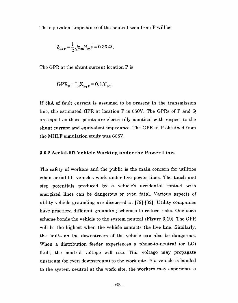
The equivalent impedance of the neutral seen from P will be

ZEq P = |>/Zn„RgnS = 0 36 Q •

The GPR at the shunt current location P is

GPRp= INZEq.P= 0.131pp.

If 5kA of fault current is assumed to be present in the transmission

line, the estimated GPR at location P is 650V. The GPRs of P and Q

are equal as these points are electrically identical with respect to the

shunt current and equivalent impedance. The GPR at P obtained from

the MHLF simulation study was 605V.

3.6.2 Aerial-lift Vehicle Working under the Power Lines

The safety of workers and the public is the main concern for utilities

when aerial-lift vehicles work under live power lines. The touch and

step potentials produced by a vehicle's accidental contact with

energized lines can be dangerous or even fatal. Various aspects of

utility vehicle grounding are discussed in [79]-[82]. Utility companies

have practiced different grounding schemes to reduce risks. One such

scheme bonds the vehicle to the system neutral (Figure 3.19). The GPR

will be the highest when the vehicle contacts the live line. Similarly,

the faults on the downstream of the vehicle can also be dangerous.

When a distribution feeder experiences a phase-to-neutral (or LG)

fault, the neutral voltage will rise. This voltage may propagate

upstream (or even downstream) to the work site. If a vehicle is bonded

to the system neutral at the work site, the workers may experience a

-62-

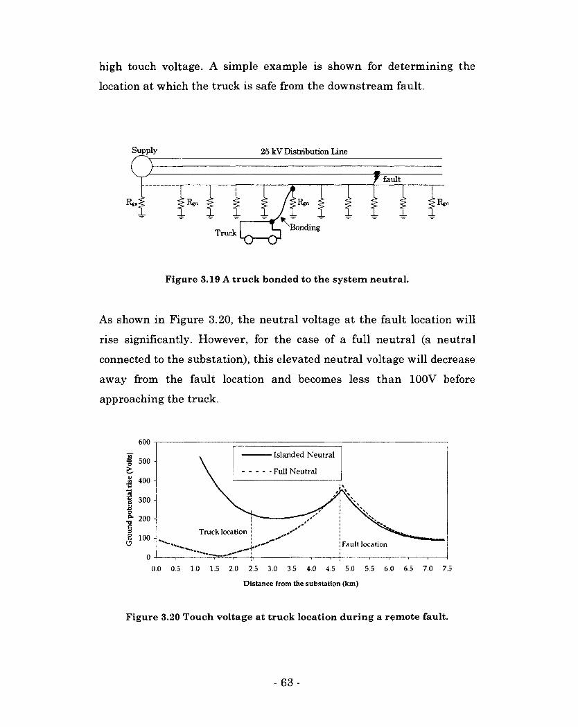
high touch voltage. A simple example is shown for determining the

location at which the truck is safe from the downstream fault.

Supply 25 kV Distribution Line

y fault

"Bonding Truck

Figure 3.19 A truck bonded to the system neutral.

As shown in Figure 3.20, the neutral voltage at the fault location will

rise significantly. However, for the case of a full neutral (a neutral

connected to the substation), this elevated neutral voltage will decrease

away from the fault location and becomes less than 100V before

approaching the truck.

600

Islanded Neutral € 500 -

Full Neutral

300 -

200 -

Truck location 100 -

Fault location

0.0 0.5 1.0 1.5 2.0 2.5 3.0 3.5 4.0 4.5 5.0 5.5 6.0 6.5 7.0 7.5

Distance from the substation (km)

Figure 3.20 Touch voltage at truck location during a remote fault.

- 63 -

However, in the case of an islanded neutral, the GPR at the upstream

ending point is higher than the GPR at the fault location. The workers

can be exposed to a higher GPR than in the case of a full neutral.

However, the worst case of GPR for a remote fault corresponds to a

truck working at the upstream ending point of the islanded neutral.

3.7 Practical Issues of Proposed Technique

The formulae derived in this chapter are based on the main

assumptions of the presence of a regular grounding interval and

identical grounding resistances. The developed formulae are applied to

SLG faults. Questions may arise about the accuracy of the results

when these assumptions are not met. Moreover, the equivalent

impedance of ZEq is assumed to be constant. These issues are addressed

in the following subsections.

3.7.1 Irregular Grounding Interval

The equivalent impedance (Zsq) is a function of the grounding interval

(s). For a practical range of grounding intervals, the variation of ZEq is

not significant. For example, Figure 3.6 reveals that the ladder

impedance increases from 1.5Q to about 1.8Q only when the grounding

interval changes from 200m to 300m. Using an average grounding

interval will have only marginal effects on the results. The voltages

induced in the neutral segments will differ if the distances between

adjacent grounding resistances are not equal. However, the equivalent

current sources are independent of the distance between two

- 64 -

grounding points (Equation 3.8). Thus, the assumption of a uniform

grounding interval is acceptable.

3.7.2 Non-identical Grounding Resistances

It is known that the grounding resistance varies as the soil resistivity

changes at various locations along the line corridor. In such cases,

neutral segments of alike grounding resistances can be grouped

together to obtain the equivalent impedance for that particular line

section and so forth. The actual GPR profiles can deviate from the

analytical ones. However, the maximum GPRs that occur at the

current injection locations can be estimated easily. Therefore, the

estimation assuming the identical grounding resistances neither

complicates the analytical process, nor affects the results significantly.

3.7.3 Line-to-Line Fault

Although the proposed model was examined by using the single-line-to-

ground (SLG) faults, the equations developed are equally applicable to

double-line-to-ground (LLG) faults. The only difference is the fault

current magnitude, which is the sum of the currents of the two phases

under fault and is usually less than the SLG fault current. The

resulting GPR will change accordingly. A separate study is not needed

to illustrate the mechanisms.

3.8 Conclusions

The GPR mechanisms were illustrated, and an analytical technique

was established to estimate the GPR. This technique is capable of

-65-

identifying and quantifying the impact of various factors such as the

grounding resistance, grounding interval and neutral conductor size.

The method developed in this chapter was applied to estimate the GPR

in a distribution line built below the transmission line. The simulation

studies confirmed the accuracy of the analytical findings. Based on the

findings of this chapter, the following conclusions can be made:

• The mutual coupling between the phase and neutral conductors

induces the voltage in the neutral conductor, which consequently

produces the GPR.

• The magnitude of the maximum GPR is dictated mainly by the

fault current through the induced neutral current and the

equivalent impedance of the MGN.

• The GPR is proportional to the equivalent impedance of the

MGN and the square-root of the grounding resistance, the

impedance of the neutral conductor, and the grounding interval.

• The maximum GPR is located at the grounded node where the

induced current source is located.

• The induced current sources are located at the ends of the

section of the neutral length exposed to the fault current.

-66-

4. Analytical Approaches to Temporary Overvoltage

Assessment

The neutral current varies in the different segments of the neutral

wire due to the groundings at multiple points along the neutral length.

One of the challenges with a MGN system is incorporating its neutral

current in the temporary overvoltage (TOV) calculation. As a result,

the mechanisms or components leading to TOV in the MGN systems

during SLG faults have not been fully analyzed, and the effect of

neutral current on TOV has not been understood. This chapter

illustrates the mechanism of TOV and analyzes the factors that affect

its magnitude. Their impacts are quantified by establishing the

approximate formulae. The findings are confirmed by the simulation

results. Sensitivity studies are performed to examine the effects of

neural grounding parameters.

4.1 Introduction

The TOV or swell is defined as an increase of rms voltage to between

1.1 and 1.8 per unit at power frequency for durations from 0.5 cycles to

1 min [10]. A simple concept of overvoltage is shown in Figure 4.1

where the phase voltage of one phase rises above the nominal voltage

during the fault on the other phase. The overvoltages are usually

associated with system fault conditions. They can also occur due to

switching off a large load, or energizing a large capacitor bank [10].

- 67-

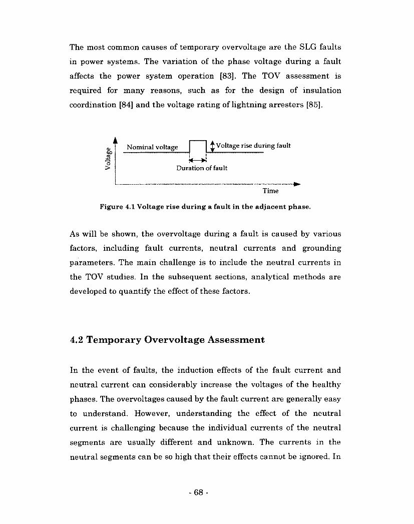
The most common causes of temporary overvoltage are the SLG faults

in power systems. The variation of the phase voltage during a fault

affects the power system operation [83]. The TOV assessment is

required for many reasons, such as for the design of insulation

coordination [84] and the voltage rating of lightning arresters [85].

<v to 2 "o >

Nominal voltage ^ Voltage rise during fault

*—•! Duration of fault

Time

Figure 4.1 Voltage rise during a fault in the adjacent phase.

As will be shown, the overvoltage during a fault is caused by various

factors, including fault currents, neutral currents and grounding

parameters. The main challenge is to include the neutral currents in

the TOV studies. In the subsequent sections, analytical methods are

developed to quantify the effect of these factors.

4.2 Temporary Overvoltage Assessment

In the event of faults, the induction effects of the fault current and

neutral current can considerably increase the voltages of the healthy

phases. The overvoltages caused by the fault current are generally easy

to understand. However, understanding the effect of the neutral

current is challenging because the individual currents of the neutral

segments are usually different and unknown. The currents in the

neutral segments can be so high that their effects cannot be ignored. In

-68-

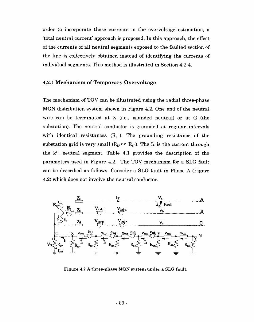
order to incorporate these currents in the overvoltage estimation, a

'total neutral current' approach is proposed. In this approach, the effect

of the currents of all neutral segments exposed to the faulted section of

the line is collectively obtained instead of identifying the currents of

individual segments. This method is illustrated in Section 4.2.4.

4.2.1 Mechanism of Temporary Overvoltage

The mechanism of TOV can be illustrated using the radial three-phase

MGN distribution system shown in Figure 4.2. One end of the neutral

wire can be terminated at X (i.e., islanded neutral) or at G (the

substation). The neutral conductor is grounded at regular intervals

with identical resistances (Rgn). The grounding resistance of the

substation grid is very small (Rgs« Rgn). The Ik is the current through

the kth neutral segment. Table 4.1 provides the description of the

parameters used in Figure 4.2. The TOV mechanism for a SLG fault

can be described as follows. Consider a SLG fault in Phase A (Figure

4.2) which does not involve the neutral conductor.

Vind- Vind:

Znn

Isub

Figure 4.2 A three-phase MGN system under a SLG fault.

- 69 -

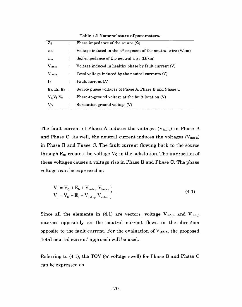
Table 4.1 Nomenclature of parameters.

Va,Vb,V(

VG

Vind-p

6nk

Zs

Znn

IF

Ea, Eb, Ei

Phase impedance of the source (£2)

Voltage induced in the kth segment of the neutral wire (V/km)

Self-impedance of the neutral wire (Q/km)

Voltage induced in healthy phase by fault current (V)

Total voltage induced by the neutral currents (V)

Fault current (A)

Source phase voltages of Phase A, Phase B and Phase C

Phase-to-ground voltage at the fault location (V)

Substation ground voltage (V)

The fault current of Phase A induces the voltages (Vind-p) in Phase B

and Phase C. As well, the neutral current induces the voltages (Vind-n)

in Phase B and Phase C. The fault current flowing back to the source

through Rgs creates the voltage VG in the substation. The interaction of

these voltages causes a voltage rise in Phase B and Phase C. The phase

voltages can be expressed as

Since all the elements in (4.1) are vectors, voltage Vind-n and Vind-p

interact oppositely as the neutral current flows in the direction

opposite to the fault current. For the evaluation of Vind-n, the proposed

'total neutral current' approach will be used.

Referring to (4.1), the TOV (or voltage swell) for Phase B and Phase C

can be expressed as

(4.1)

- 70 -

VtOV _ + Xnd-p"înd-n • (4-2)

The three components of (4.2) are individually computed in the

following subsections.

4.2.2 Substation Neutral Voltage Rise

The first component, the substation neutral voltage rise (Vg), is the

product of the amount of fault current returning to the substation and

grounding resistance of substation Rgs, which is given by

Y3 ~ "URgs > (4.3)

where ISub is the current that flows through Rgs. The highest possible

amount of this current is equal to the fault current (IF) when the

neutral conductor is isolated from the substation. Therefore, the

maximum substation neutral voltage rise is given as

Vo islandN — "^F^gs • (4-4)

When the neutral is terminated in the substation, the Isub is

approximately given by IF-II; then

Va-fuiiN — "^F ~~ Ii)R„ • (4.5)

As shown in Chapter 2, II is about 35% of IF- Then the substation GPR

will be 35% less than that of the islanded neutral case.

- 71 -

4.2.3 Voltage Induced by Fault Current

The component Vind-P in (4.2) is the voltage induced by the fault current

in the healthy phases (B and C) through mutual impedances. This

voltage is given by

where

d = the fault distance from substation (km)

Zmp = the phase-to-phase mutual impedance (Q/km)

ZSM = the source mutual impedance (Q)

IF = the fault current (A).

4.2.4 Voltage Induced by Neutral Current

Again, consider the neutral circuit of Figure 4.2 where the voltages

induced in the neutral conductor by the fault current are also shown.

The neutral section downstream of the fault location does not have any

induced voltages. The total voltage induced in a phase conductor by

neutral current is given by

VIND-P - (ZSM +Zmpd)lF> (4-6)

Vmd-n = -GlZmn + l2Zmn + I3Zmn + ) = "Lm2: sum mn > (4.7)

where

I sum 2X for all k

Now the goal is to find I8um. The voltage VNF is expressed as sum.

- 72 -

sum' sum nn

I 1

(V-V^d) , (4.8) sum z nn

where

(4-9)

Equation (4.8) has a special meaning. The unknown variables on the

right-hand side of the equation are the GPRs at the fault location and

upstream end of the neutral wire (or substation), which can be

obtained by the method developed in Chapter 3. Thus, the sum of the

currents of the neutral segments is obtained by substituting these GPR

values as shown below.

Case 1: Neutral Terminated in the Substation

In this case, the voltage drop in the substation grounding resistance is

very small such that VG « VNF (typical Rgs ~ 0.15Q). Then from (4.9),

"'•sum _ (^NF + en^)^Znn

where

VNF = -iNz N Eq-F •

Then

= (-IwZP„ F + e„d)/zn„ sum \ N bq*r n / nn

~ ( Êq F/Znn +^N^)

Isum = (-Êq F/Znn + * (4.10)

- 73 -

Thus, the voltage induced by the neutral current will be

v ind-n sum

(4.11) nn

Case 2: Neutral Isolated from the Substation

For the islanded case, the neutral terminates at X, affecting the

amount of current flowing in the neutral segments, so the ISum needs to

be recalculated. By replacing the VG by VNX in (4.8), the total current

becomes

As the equivalent impedance at X is two times the equivalent

impedance of F, the GPR at X will be two times larger than the GPR at

F. However, the polarity is opposite; i.e., VNX= -2VNF- Substituting VNF

= -iNZEq-F in Equation (4.12),

U = — (VNF-V N X + e„d) . z

(4.12)

^sum ~~ ( ^Êq-F/Znn + * (4.13)

The voltage induced by the neutral current will be

ind-n sum mn nn

(4.14)

which is less than the value given by (4.11).

- 74-

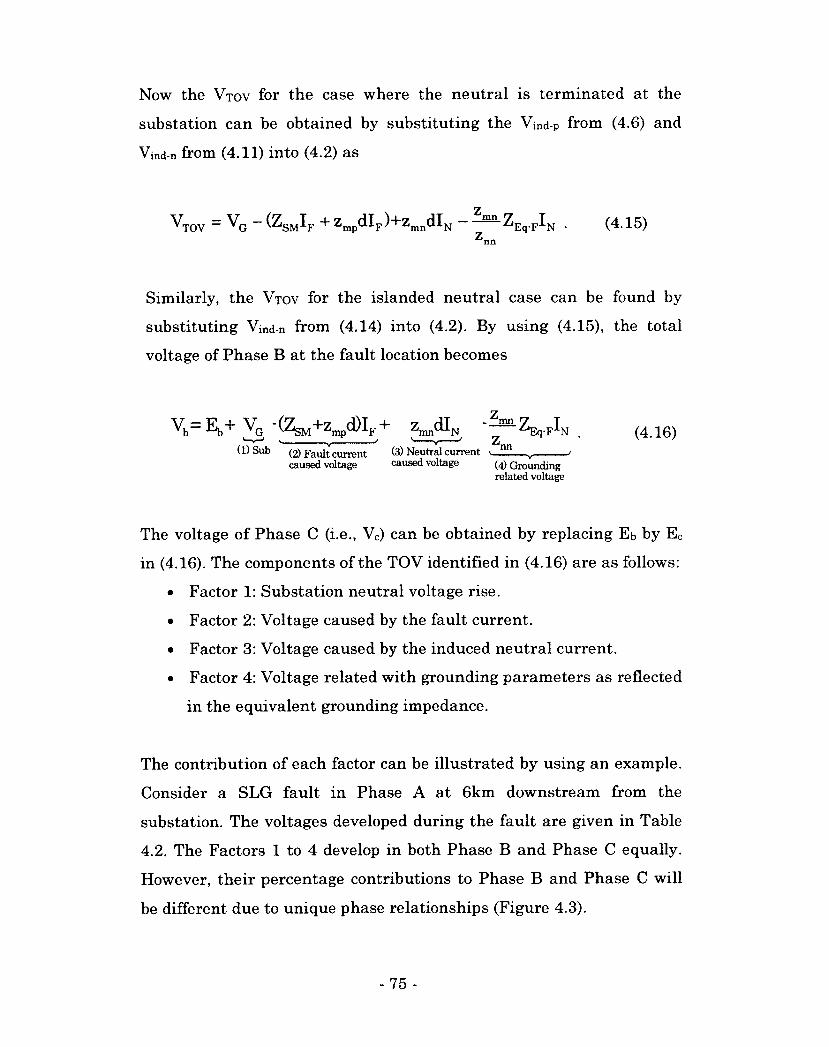
Now the VTOV for the case where the neutral is terminated at the

substation can be obtained by substituting the Vind-p from (4.6) and

Vind-n from (4.11) into (4.2) as

Vtov = ^G ~ ^SM^F + Zmp^F^Zmn^N ÊqF^N • (4.15) Znn

Similarly, the VTOV for the islanded neutral case can be found by

substituting Vind-n from (4.14) into (4.2). By using (4.15), the total

voltage of Phase B at the fault location becomes

^b-Eh+ Vq "(ZSM+zmpd)IF+ zmndIN " J™ _ (4.16) 1 » v i v v

(1) Sub (2) Fault current (3) Neutral current » „ caused voltage caused voltage (4) Grounding

related voltage

The voltage of Phase C (i.e., Vc) can be obtained by replacing EB by EC

in (4.16). The components of the TOV identified in (4.16) are as follows:

• Factor 1: Substation neutral voltage rise.

• Factor 2: Voltage caused by the fault current.

• Factor 3: Voltage caused by the induced neutral current.

• Factor 4: Voltage related with grounding parameters as reflected

in the equivalent grounding impedance.

The contribution of each factor can be illustrated by using an example.

Consider a SLG fault in Phase A at 6km downstream from the

substation. The voltages developed during the fault are given in Table

4.2. The Factors 1 to 4 develop in both Phase B and Phase C equally.

However, their percentage contributions to Phase B and Phase C will

be different due to unique phase relationships (Figure 4.3).

- 75 -

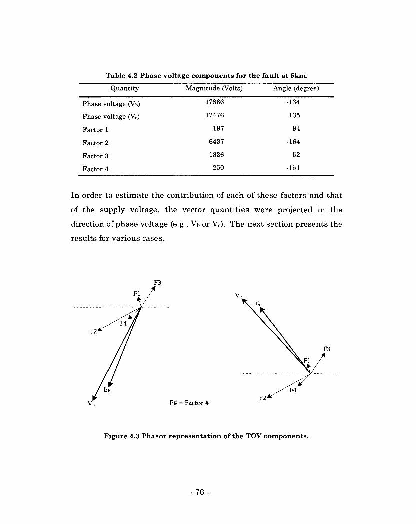
Table 4.2 Phase voltage components for the fault at 6km.

Quantity Magnitude (Volts) Angle (degree)

Phase voltage (Vb) 17866 -134

Phase voltage (Vc) 17476 135

Factor 1 197 94

Factor 2 6437 -164

Factor 3 1836 52

Factor 4 250 -151

In order to estimate the contribution of each of these factors and that

of the supply voltage, the vector quantities were projected in the

direction of phase voltage (e.g., Vb or Vc). The next section presents the

results for various cases.

F3

F2

Figure 4.3 Phasor representation of the TOY components.

- 76-

4.3 Analytical and Simulation Results

The system and data described in Chapter 3 were used for this study

as well. Tables 4.3-4.4 show the individual components in the

percentage of the phase voltages at different fault locations for Phase B

and Phase C, respectively. As these tables reveal, the contribution level

of a particular factor is different for Phase B and Phase C voltages

because that factor is separated from the phase voltages with a unique

displacement angle as shown in Figure 4.3.

Among the four factors, the biggest contributor is Factor 2 (i.e., the

coupling between phase conductors). Its contribution increases with

the increase in fault distance because the length of fault exposure of

the phase conductor increases. The contribution of this factor to Vb is

greater than that to Vc. Another significant contributor is Factor 3,

which is related to the coupling with neutral current. Its contribution

also increases in a negative direction with fault distance or exposure

length. The differences in effects of this factor on Phase B and Phase C

voltages are due to its orientation as illustrated in the phasor diagram

(Figure 4.3). Factor 1 (i.e., VG) has the least impact in the case of

Phase B and Factor 4 has the least impact in the case of Phase C,

generally below 2%. The fourth factor is also small.

Table 4.3 Percentage contribution of individual factors to Vb.

Fault (km) Vb(pu) Eb (%) Factor 1 Factor 2 Factor 3 Factor 4

2 1.190 81.6 -1.8 23.8 -6.2 2.3

4 1.220 79.4 -1.2 28.7 -8.9 1.7

6 1.238 78.2 -0.9 31.4 -10.1 1.3

8 1.250 77.5 -0.7 33.0 -11.0 1.1

10 1.258 76.6 -0.6 34.1 -11.6 0.9

- 77-

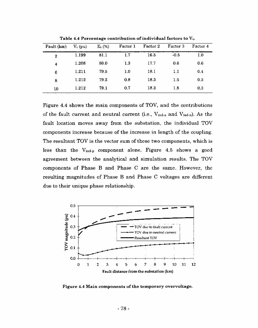
Table 4.4 Percentage contribution of individual factors to Vc.

Fault (km) Vc (pu) Ec (%) Factor 1 Factor 2 Factor 3 Factor 4

2 1.199 81.1 1.7 16.5 -0.5 1.0

4 1.208 80.0 1.3 17.7 0.6 0.6

6 1.211 79.5 1.0 18.1 1.1 0.4

8 1.212 79.2 0.8 18.3 1.5 0.3

10 1.212 79.1 0.7 18.3 1.8 0.3

Figure 4.4 shows the main components of TOV, and the contributions

of the fault current and neutral current (i.e., Vind-a and Vind-n). As the

fault location moves away from the substation, the individual TOV

components increase because of the increase in length of the coupling.

The resultant TOV is the vector sum of these two components, which is

less than the Vind-p component alone. Figure 4.5 shows a good

agreement between the analytical and simulation results. The TOV

components of Phase B and Phase C are the same. However, the

resulting magnitudes of Phase B and Phase C voltages are different

due to their unique phase relationship.

0.5

1? 0.4 -•£>

0.4 -0)

•o 2 0.3 -

1 / £ 0.2 -

> O H 0.1 -

• TOV due to fault current

-TOV due to neutral current

•Resultant TOV

+

2 3 4 5 6 7 8 9 1 0


11 12

Figure 4.4 Main components of the temporary overvoltage.

- 78-

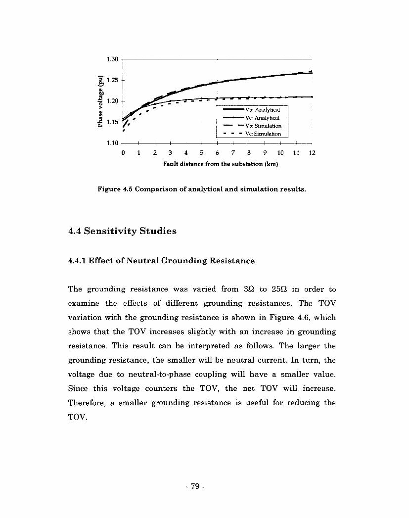
1.30

g. 1-25 -

3 1-20 -

Vb: Analytical -• Vc: Analytical " •— Vb: Simulation " " Vc: Simulation

rfi 1.15

1.10

0 2 3 5 7 1 4 6 8 9 10 11 12


Figure 4.5 Comparison of analytical and simulation results.

4.4 Sensitivity Studies

4.4.1 Effect of Neutral Grounding Resistance

The grounding resistance was varied from 3£2 to 25Q in order to

examine the effects of different grounding resistances. The TOV

variation with the grounding resistance is shown in Figure 4.6, which

shows that the TOV increases slightly with an increase in grounding

resistance. This result can be interpreted as follows. The larger the

grounding resistance, the smaller will be neutral current. In turn, the

voltage due to neutral-to-phase coupling will have a smaller value.

Since this voltage counters the TOV, the net TOV will increase.

Therefore, a smaller grounding resistance is useful for reducing the

TOV.

- 79-

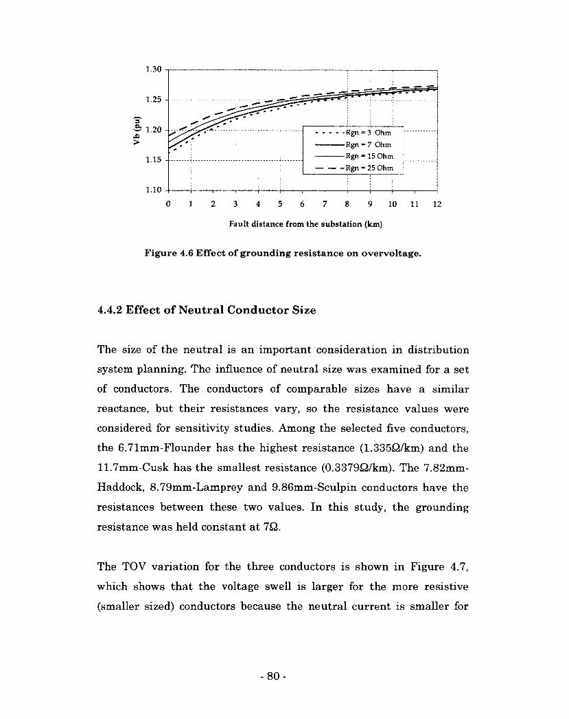
1.30

1.25 -

& 1.20 < •® "V/ — • Rgn = 3 Ohm

— Rgn = 7 Ohm

— Rgn = 15 Ohm

• - Rgn = 25 Ohm 1.15 -

1.10

0 1 2 3 4 5 7 6 8 9 10 11 12


Figure 4.6 Effect of grounding resistance on overvoltage.

4.4.2 Effect of Neutral Conductor Size

The size of the neutral is an important consideration in distribution

system planning. The influence of neutral size was examined for a set

of conductors. The conductors of comparable sizes have a similar

reactance, but their resistances vary, so the resistance values were

considered for sensitivity studies. Among the selected five conductors,

the 6.71mm-Flounder has the highest resistance (1.335£2/km) and the

11.7mm-Cusk has the smallest resistance (0.3379Q/km). The 7.82mm-

Haddock, 8.79mm-Lamprey and 9.86mm-Sculpin conductors have the

resistances between these two values. In this study, the grounding

resistance was held constant at 7Q.

The TOV variation for the three conductors is shown in Figure 4.7,

which shows that the voltage swell is larger for the more resistive

(smaller sized) conductors because the neutral current is smaller for

-80-

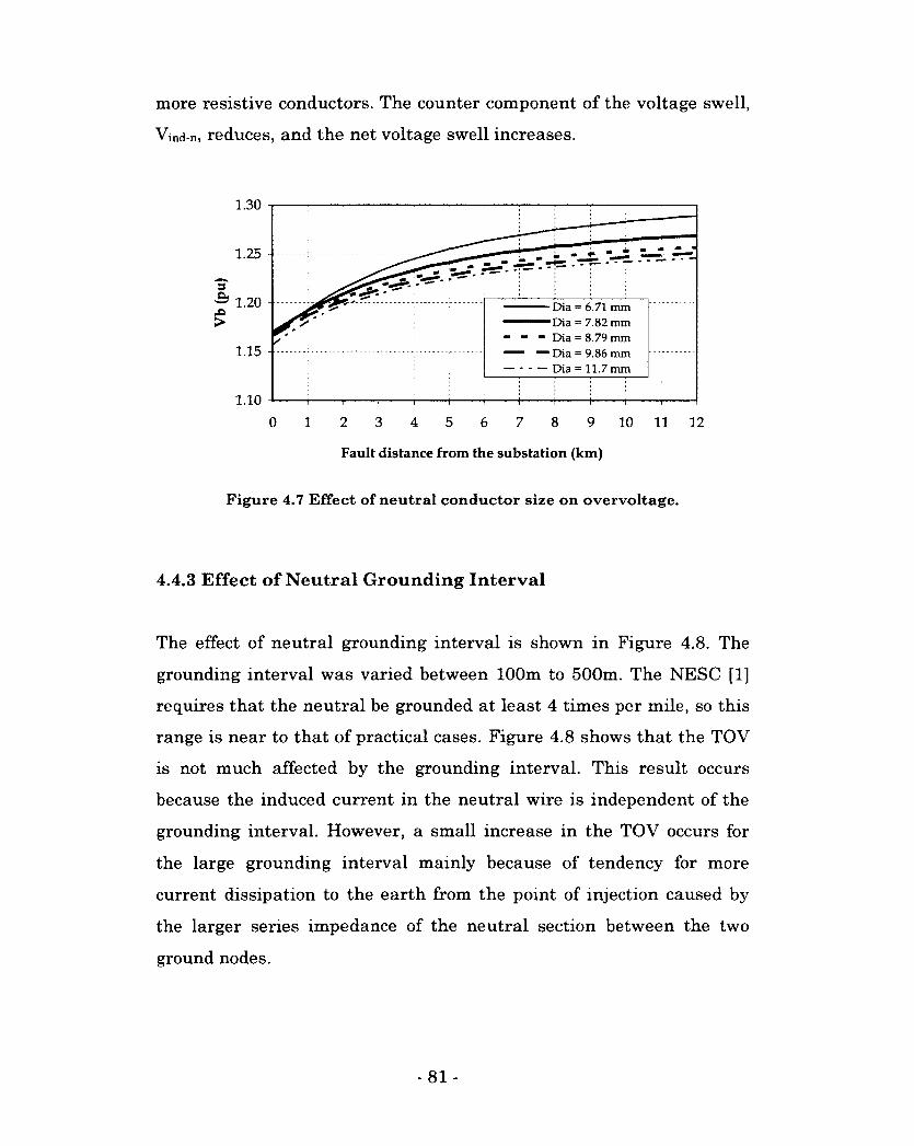
more resistive conductors. The counter component of the voltage swell,

Vind-n, reduces, and the net voltage swell increases.

1.30

1.25 -

•=> 1.20 - Dia = 6.71 mm 1 Dia = 7.82 mm

" ~ Dia = 8.79 mm " — Dia = 9.86 mm - - — Dia = 11.7 mm

1.15 -

1.10 4

0 2 3 4 5 7 8 9 10 11 12 1 6


Figure 4.7 Effect of neutral conductor size on overvoltage.

4.4.3 Effect of Neutral Grounding Interval

The effect of neutral grounding interval is shown in Figure 4.8. The

grounding interval was varied between 100m to 500m. The NESC [1]

requires that the neutral be grounded at least 4 times per mile, so this

range is near to that of practical cases. Figure 4.8 shows that the TOV

is not much affected by the grounding interval. This result occurs

because the induced current in the neutral wire is independent of the

grounding interval. However, a small increase in the TOV occurs for

the large grounding interval mainly because of tendency for more

current dissipation to the earth from the point of injection caused by

the larger series impedance of the neutral section between the two

ground nodes.

- 81 -

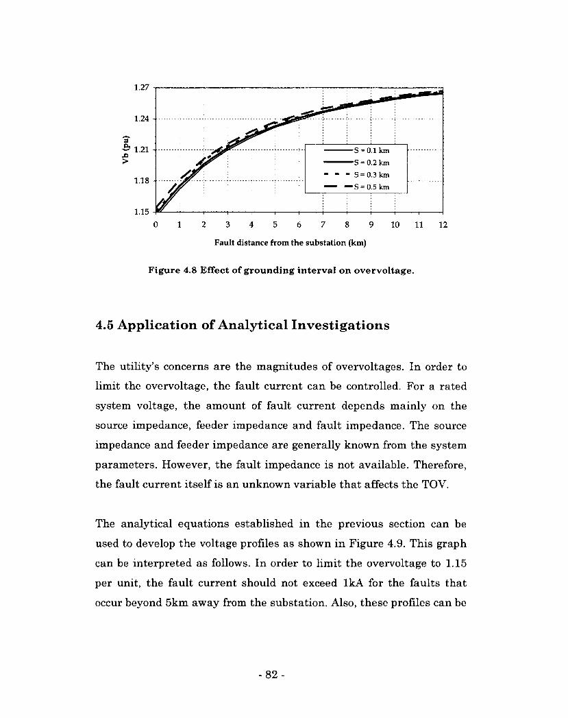
1.27

1.24

— 1.21 S = 0.1 km

S = 0.2 km

" " S = 0.3 km

" — S = 0.5 km 1.18 -

1.15 -I 0 1 2 3 7 4 5 6 8 9 10 11 12


Figure 4.8 Effect of grounding interval on overvoltage.

4.5 Application of Analytical Investigations

The utility's concerns are the magnitudes of overvoltages. In order to

limit the overvoltage, the fault current can be controlled. For a rated

system voltage, the amount of fault current depends mainly on the

source impedance, feeder impedance and fault impedance. The source

impedance and feeder impedance are generally known from the system

parameters. However, the fault impedance is not available. Therefore,

the fault current itself is an unknown variable that affects the TOV.

The analytical equations established in the previous section can be

used to develop the voltage profiles as shown in Figure 4.9. This graph

can be interpreted as follows. In order to limit the overvoltage to 1.15

per unit, the fault current should not exceed lkA for the faults that

occur beyond 5km away from the substation. Also, these profiles can be

-82-

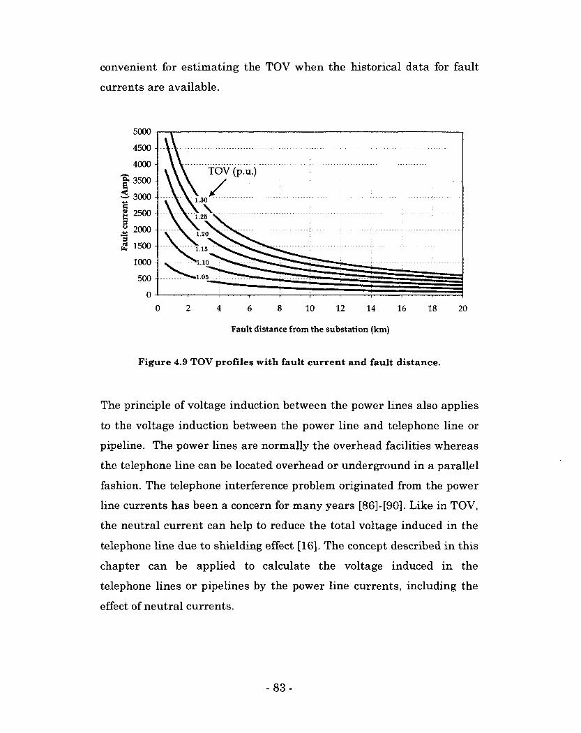
convenient for estimating the TOV when the historical data for fault

currents are available.

5000

4500

4000 TOV (p.u.)

"S E <

3500

3000 1.30 c a s u

2500 1.25

_ 2000

| 1500 1.20

1.15

1000 '1.10

.1.05 500

2 4 8 0 6 10 12 14 16 18 20


Figure 4.9 TOV profiles with fault current and fault distance.

The principle of voltage induction between the power lines also applies

to the voltage induction between the power line and telephone line or

pipeline. The power lines are normally the overhead facilities whereas

the telephone line can be located overhead or underground in a parallel

fashion. The telephone interference problem originated from the power

line currents has been a concern for many years [86]-[90]. Like in TOV,

the neutral current can help to reduce the total voltage induced in the

telephone line due to shielding effect [16]. The concept described in this

chapter can be applied to calculate the voltage induced in the

telephone lines or pipelines by the power line currents, including the

effect of neutral currents.

-83-

4.6 Conclusions

In this chapter, the temporary overvoltage (TOV) mechanism was

illustrated and the analytical technique was developed to calculate the

TOV. The "total neutral current" approach was introduced to include

the neutral currents in calculations. This method distinguishes the

overvoltage contributions of various factors such as the fault current

and neutral current. The analytical results were confirmed through the

simulation studies. The following are the main conclusions:

• The voltages induced by the fault current and the neutral

current are the most decisive factors for the TOV. While the

fault current caused about 30% to the TOV, the neutral current

compensated by about 10%. Therefore, the neutral currents

should be included in the overvoltage calculation.

• The substation neutral voltage contributed less than 2% when

the substation grounding resistance is 0.15Q.

• The neutral grounding parameters such as the grounding

resistance and grounding interval also have a small impact on

the TOV.

The concept of the total neutral current approach proposed in this

chapter can be also applied to calculate the voltage induction in the

nearby parallel conductors such as the pipelines and telephone cables.

The finding of neutral current effects is significant in the study of the

power-line-to-telephone interference problem.

- 84-

5. A Novel Approach to Stray Voltage Contribution

Determination

The incorrect usage of stray-voltage-related terms has created

confusion. As well, several factors are responsible for stray voltage

problems. After defining stray-voltage-related terms and briefly

discussing the causes of stray voltage, this chapter illustrates the

mechanism of stray voltage generation. The utility is generally blamed

for the stray voltage problems in a customer facility because the high

NEV of the MGN (utility circuit) propagates to the customer circuit. In

this chapter, a measurement-based approach is proposed for

distinguishing the stray voltage contributions of the utility (off-site

source) and customer (on-site source). The feasibility of the proposed

method is verified through analytical studies, simulations and field

tests. The potential applications of the method are investigated, and

various implementation issues are clarified.

5.1 Introduction

Stray voltage has been a danger to farm livestock for many years.

Animals are more susceptible to problems associated with stray voltage

than humans due to their physiological differences. Therefore, stray

voltage studies have been carried out on animals such as cows, pigs,

sheep, and poultry [61],[91]-[94].

- 85 -

In recent years, complaints of stray-voltage-related problems involving

humans have become more frequent. For instance, cases of an

electrical sensation felt when showering, and a tingling sensation felt

when entering and exiting swimming pools have been reported.

Investigations revealed that these problems originated from the bare

corroded concentric neutral of the distribution system. Stray voltage

has been blamed for similar electrical phenomena that commonly occur

in metallic fences, street lights or utility poles, and underground

manholes. However, these phenomena could have been caused by

something else, such as contact voltage, step or touch voltage and

static discharge. To appreciate the difference between stray voltage

and other phenomena that are incorrectly referred to as stray voltages,

the definitions must be reviewed so that the actual sources of stray

voltage can be understood.

5.1.1 Terms and Definitions

The terms commonly associated with stray-voltage-related electrical

phenomena are defined as follows:

Stray voltage: Generally, it refers to a small voltage, not exceeding

about 10V, due mainly to return currents originating from an

unbalanced load during the normal operations of power delivery.

Stray voltages are significantly less than the voltages considered

dangerous by the National Electrical Safety Code [1], which sets

the limit at 50V. Therefore, stray voltage is not considered lethal.

Stray current: Some people use this term to refer to the situation in

which any current is entering the earth, because they believe that

-86-

the current, not the voltage, causes death [57], In fact, however,

the current is created from the stray voltage.

Touch voltage: This is the potential difference between the ground

potential rise (GPR) of a grounded structure and the surface

potential at the point where a person is standing while at the same

time touching that grounded structure [19]. The touch voltage is

related to the faults in the system. A person can experience touch

voltage between a hand and a foot.

Step voltage: This is the difference in surface potential experienced

by a person bridging a distance of lm with his/her feet without

contacting any other grounded object [19]. Step voltage is also

associated with the faults in the system. This voltage can occur

between the two feet of an individual during a fault.

Contact voltage: Contact voltage occurs in places similar to those of

stray voltage, but can be dangerous and can result in death. This

voltage is a result of faults in the system [19] and can arise from

improper wiring, a fault or leakage current. Using a neutral

conductor as a ground wire, or interchanging the neutral and phase

wires in the connections are examples of incorrect wiring. The

voltages originating from equipment faults and damaged insulation

of the conductor or equipment fall under this category.

Static discharge: Static electricity is usually produced by friction,

i.e., when two materials are rubbed together. A person may

experience an electrical shock when he or she touches an object,

and static electricity suddenly discharges. This phenomenon does

not occur with stray voltage [57].

- 87 -

5.1.2 Main Causes of Stray Voltage

The first step in the investigation of the stray voltage problem is to

identify its major causes. Its main cause is the voltage that develops on

a grounded neutral wiring network of a power delivery system (a

primary circuit) and/or a power utilization system (a secondary circuit)

due to the primary return current, secondary return current and power

system induced current [7]. Grounding is provided to keep the voltage

potential between the neutral system and the earth below levels that

could be harmful to people or animals [17]. Thus, the voltage potentials

in the primary and secondary neutral circuits are the main causes of

stray voltage. Such voltage potentials may arise for a variety of

reasons, including the following:

• Unbalanced single-phase loads in the secondary system.

• Excessive neutral current in the primary feeder.

• High resistance or loose connections.

• High resistance in the neutral conductor.

• Inductive coupling between the neutral wire and the energized

parallel conductors in the primary system.

• Excessive harmonics in the system.

The secondary circuit consists of two phase wires and a neutral. Some

loads are connected between the first phase wire and the neutral, some

are connected between the second phase wire and the neutral, and the

other loads are connected between the two phases. Normally, the group

of loads in one phase is not equal to the group of loads in the other

phase. Therefore, the current resulting from this unbalanced load will

flow into the neutral of the secondary system. High resistance in the

neutral wire prevents this current from returning through the neutral

wire, so more current is diverted to the ground, creating high stray

- 88 -

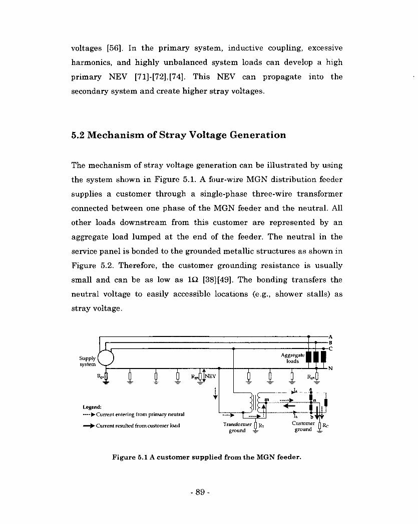
voltages [56], In the primary system, inductive coupling, excessive

harmonics, and highly unbalanced system loads can develop a high

primary NEV [71]-[72],[74]. This NEV can propagate into the

secondary system and create higher stray voltages.

5.2 Mechanism of Stray Voltage Generation

The mechanism of stray voltage generation can be illustrated by using

the system shown in Figure 5.1. A four-wire MGN distribution feeder

supplies a customer through a single-phase three-wire transformer

connected between one phase of the MGN feeder and the neutral. All

other loads downstream from this customer are represented by an

aggregate load lumped at the end of the feeder. The neutral in the

service panel is bonded to the grounded metallic structures as shown in

Figure 5.2. Therefore, the customer grounding resistance is usually

small and can be as low as in [38] [49]. The bonding transfers the

neutral voltage to easily accessible locations (e.g., shower stalls) as

stray voltage.

Aggregate loads Supply

system

•A B

•C

N

a

Legend: • Current entering from primary neutral

Transformer ground I* cg~ifc Customer Current resulted from customer load

Figure 5.1 A customer supplied from the MGN feeder.

- 89-

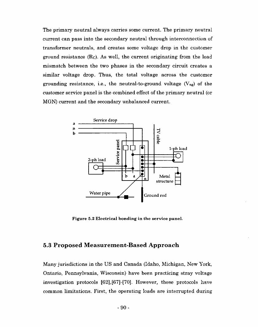
The primary neutral always carries some current. The primary neutral

current can pass into the secondary neutral through interconnection of

transformer neutrals, and creates some voltage drop in the customer

ground resistance (Rc). As well, the current originating from the load

mismatch between the two phases in the secondary circuit creates a

similar voltage drop. Thus, the total voltage across the customer

grounding resistance, i.e., the neutral-to-ground voltage (Vng) of the

customer service panel is the combined effect of the primary neutral (or

MGN) current and the secondary unbalanced current.

Service drop

1-ph load

2-ph load

Metal structure

Water pipe Ground rod

DP

Figure 5.2 Electrical bonding in the service panel.

5.3 Proposed Measurement-Based Approach

Many jurisdictions in the US and Canada (Idaho, Michigan, New York,

Ontario, Pennsylvania, Wisconsin) have been practicing stray voltage

investigation protocols [62],[67]-[70]. However, these protocols have

common limitations. First, the operating loads are interrupted during

-90-

the test, but such an interruption is not desirable. Second, one or more

proxy loads such as a portable load box are required. Finally, these

approaches need to measure the stray voltage even during the

preliminary assessment for which the relative contributions of the

utility and customer are sufficient. Measuring a stray voltage requires

a reference ground, which is generally provided by using a temporary

ground rod. In some cases, driving a temporary ground rod is difficult

or sometimes not feasible.

In this thesis, a novel idea is proposed for distinguishing the on-site

and off-site sources of the stray voltage in a customer facility. The

primary goal is to identify whether the stray voltage source is located

within or outside the customer facility by measuring the currents only.

The secondary goal is to investigate the potential applications for

helping to pinpoint the parameters, such as the grounding resistance

or neutral conductor, responsible for the stray voltage problem. The

stray voltage is included in the measurement for the same purpose. In

order to achieve these goals, a method is established by performing the

following main tasks:

• The concept of decoupling the neutral current into two

components (utility-component and customer-component) is

introduced. To decouple the neutral current, an analytical model

is developed based on the concept of the current return ratio (K).

• Based on the analytical model, a measurement-based technique is

proposed to determine the ratio K. Subsequently, the

contributions of the utility and customer are calculated.

• The proposed method was verified through simulation and tested

by using the field results.

-91 -

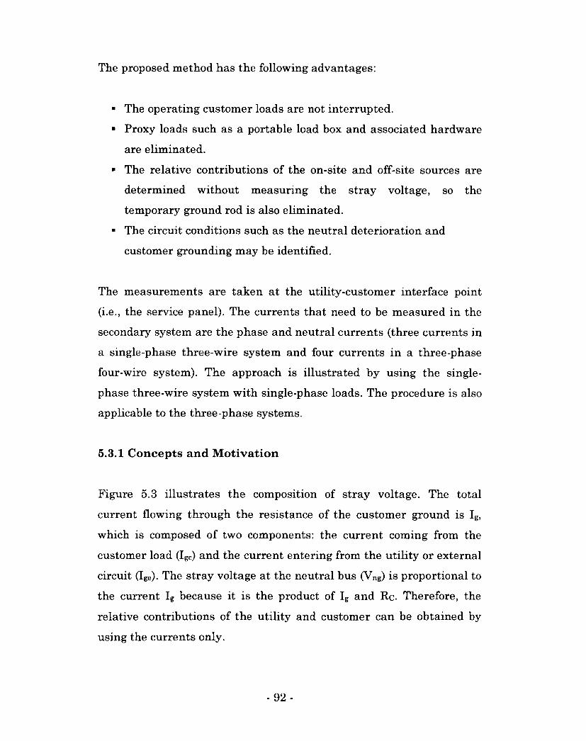
The proposed method has the following advantages:

• The operating customer loads are not interrupted.

• Proxy loads such as a portable load box and associated hardware

are eliminated.

• The relative contributions of the on-site and off-site sources are

determined without measuring the stray voltage, so the

temporary ground rod is also eliminated.

• The circuit conditions such as the neutral deterioration and

customer grounding may be identified.

The measurements are taken at the utility-customer interface point

(i.e., the service panel). The currents that need to be measured in the

secondary system are the phase and neutral currents (three currents in

a single-phase three-wire system and four currents in a three-phase

four-wire system). The approach is illustrated by using the single-

phase three-wire system with single-phase loads. The procedure is also

applicable to the three-phase systems.

5.3.1 Concepts and Motivation

Figure 5.3 illustrates the composition of stray voltage. The total

current flowing through the resistance of the customer ground is Ig,

which is composed of two components: the current coming from the

customer load (Igc) and the current entering from the utility or external

circuit (Ige). The stray voltage at the neutral bus (Vng) is proportional to

the current Ig because it is the product of Ig and Re- Therefore, the

relative contributions of the utility and customer can be obtained by

using the currents only.

- 92 -

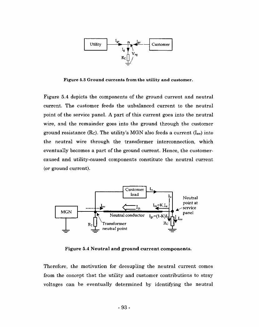
Utility Customer

Figure 5.3 Ground currents from the utility and customer.

Figure 5.4 depicts the components of the ground current and neutral

current. The customer feeds the unbalanced current to the neutral

point of the service panel. A part of this current goes into the neutral

wire, and the remainder goes into the ground through the customer

ground resistance (Rc). The utility's MGN also feeds a current (Ine) into

the neutral wire through the transformer interconnection, which

eventually becomes a part of the ground current. Hence, the customer-

caused and utility-caused components constitute the neutral current

(or ground current).

MGN

Customer load

I u >

Iu

C=In Inc=K.Iu

^ Neutral conductor lgc=(l-K)Iu

Transformer Rc RTIj

Neutral point at service panel

1 neutral point

»J | ! T

Figure 5.4 Neutral and ground current components.

Therefore, the motivation for decoupling the neutral current comes

from the concept that the utility and customer contributions to stray

voltages can be eventually determined by identifying the neutral

- 93 -

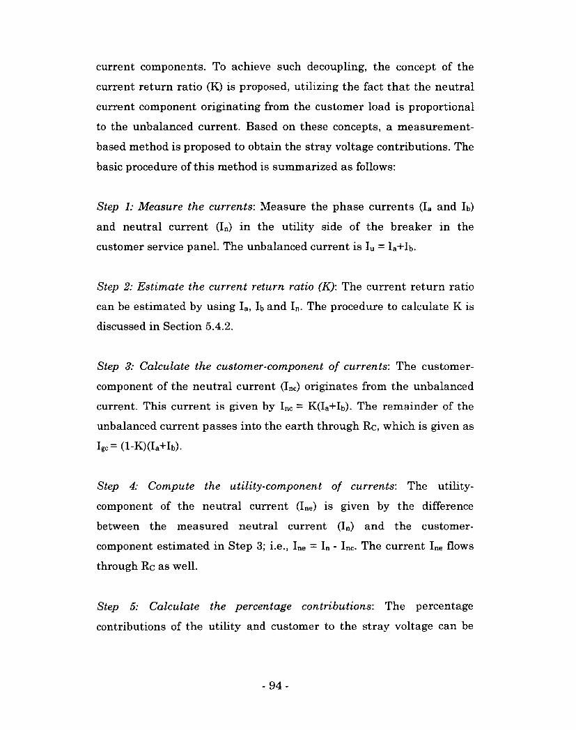
current components. To achieve such decoupling, the concept of the

current return ratio (K) is proposed, utilizing the fact that the neutral

current component originating from the customer load is proportional

to the unbalanced current. Based on these concepts, a measurement-

based method is proposed to obtain the stray voltage contributions. The

basic procedure of this method is summarized as follows:

Step 1: Measure the currents: Measure the phase currents (Ia and lb)

and neutral current (In) in the utility side of the breaker in the

customer service panel. The unbalanced current is Iu = Ia+Ib.

Step 2: Estimate the current return ratio (K): The current return ratio

can be estimated by using Ia, lb and In. The procedure to calculate K is

discussed in Section 5.4.2.

Step 3: Calculate the customer-component of currents: The customer-

component of the neutral current (Inc) originates from the unbalanced

current. This current is given by Inc — K(Ia+Ib). The remainder of the

unbalanced current passes into the earth through Rc, which is given as

Igc= (l-K)(Ia+Ib).

Step 4: Compute the utility-component of currents: The utility-

component of the neutral current (Ine) is given by the difference

between the measured neutral current (In) and the customer-

component estimated in Step 3; i.e., Ine = In - Inc. The current Ine flows

through Rc as well.

Step 5: Calculate the percentage contributions: The percentage

contributions of the utility and customer to the stray voltage can be

-94-

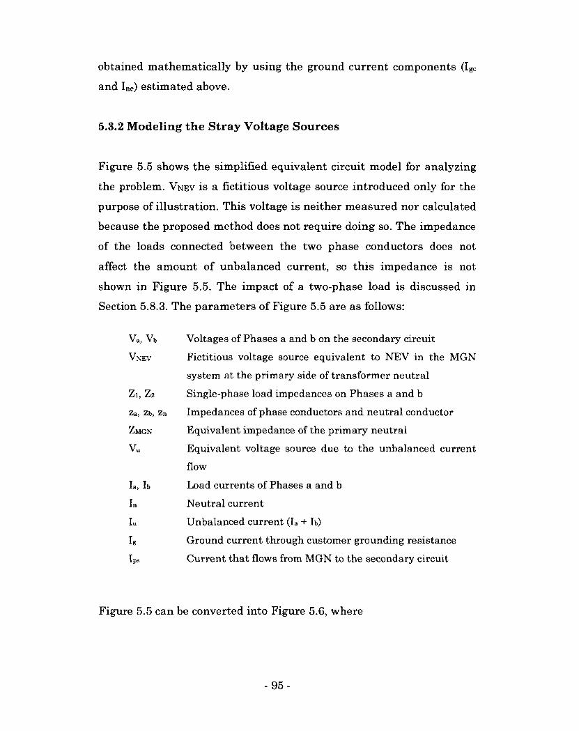
obtained mathematically by using the ground current components (Igc

and Ine) estimated above.

5.3.2 Modeling the Stray Voltage Sources

Figure 5.5 shows the simplified equivalent circuit model for analyzing

the problem. VNEV is a fictitious voltage source introduced only for the

purpose of illustration. This voltage is neither measured nor calculated

because the proposed method does not require doing so. The impedance

of the loads connected between the two phase conductors does not

affect the amount of unbalanced current, so this impedance is not

shown in Figure 5.5. The impact of a two-phase load is discussed in

Section 5.8.3. The parameters of Figure 5.5 are as follows:

Va, Vb Voltages of Phases a and b on the secondary circuit

VNEV Fictitious voltage source equivalent to NEV in the MGN

system at the primary side of transformer neutral

ZI, Z2 Single-phase load impedances on Phases a and b

za, Zb, zn Impedances of phase conductors and neutral conductor

ZMGN Equivalent impedance of the primary neutral

Vu Equivalent voltage source due to the unbalanced current

flow

la, lb Load currents of Phases a and b

In Neutral current

Iu Unbalanced current (Ia + lb)

Ig Ground current through customer grounding resistance

Ips Current that flows from MGN to the secondary circuit

Figure 5.5 can be converted into Figure 5.6, where

- 95-

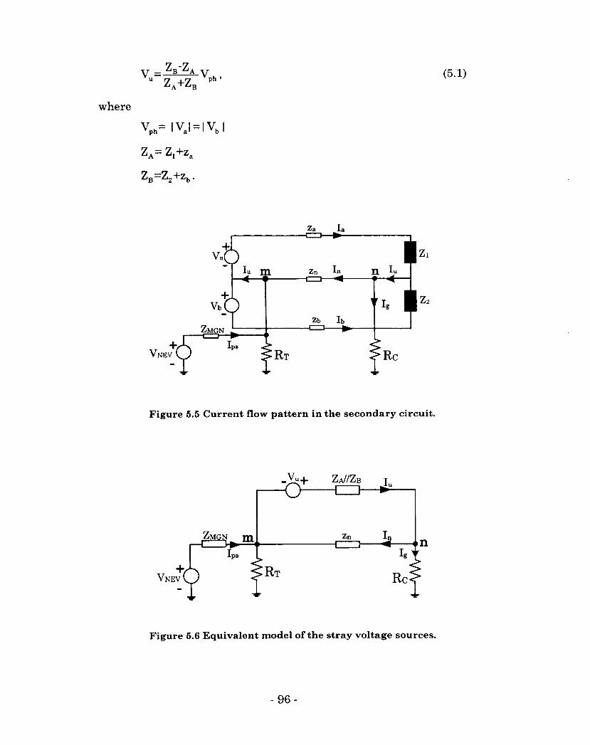
y - Zb'Za y (5 y

" ZA+ZB

where

VP H=IVJ = |VB |

ZA= Zi+za

^B—^2~*"Zb *

Za

Zn

ZMGN

VNEV RT RC

Figure 5.5 Current flow pattern in the secondary circuit.

ZMGN M

p®

-Vu+ ZA//ZB T -<>—tb—

Zn In

VNEV^P • RT Rc«

n

Figure 5.6 Equivalent model of the stray voltage sources.

- 96-

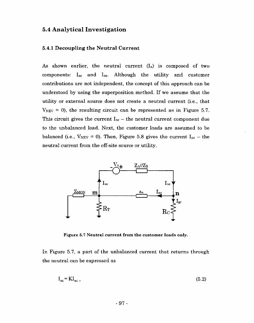
5.4 Analytical Investigation

5.4.1 Decoupling the Neutral Current

As shown earlier, the neutral current (In) is composed of two

components: Inc and Ine. Although the utility and customer

contributions are not independent, the concept of this approach can be

understood by using the superposition method. If we assume that the

utility or external source does not create a neutral current (i.e., that

VNEV = 0), the resulting circuit can be represented as in Figure 5.7.

This circuit gives the current Inc — the neutral current component due

to the unbalanced load. Next, the customer loads are assumed to be

balanced (i.e., VNEV = 0). Then, Figure 5.8 gives the current Ine - the

neutral current from the off-site source or utility.

ZA//ZB

UC

ZMGN m zn nc

RT RC

Figure 5.7 Neutral current from the customer loads only.

In Figure 5.7, a part of the unbalanced current that returns through

the neutral can be expressed as

I „c= KI U C ) (5.2)

- 97 -

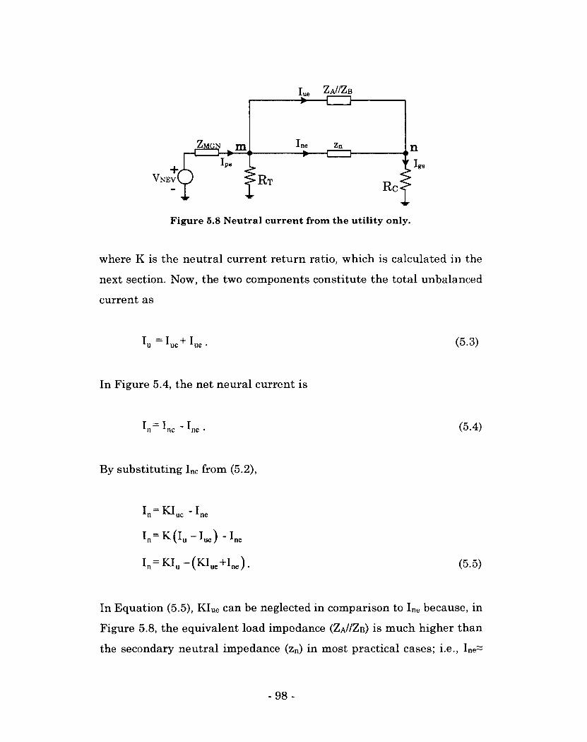
Iue ZA//ZB "• 1 I"

ZMGN m -*—•

4y VNEVV

I PB

Ine Zn n t Ige

•RT RC-

Figure 5.8 Neutral current from the utility only.

where K is the neutral current return ratio, which is calculated in the

next section. Now, the two components constitute the total unbalanced

current as

Iu luc+ ûe (5.3)

In Figure 5.4, the net neural current is

^nc " ^ne (5.4)

By substituting Inc from (5.2),

T = KT - T An ^*uc ~ ne

K(I U Iue) " ̂ ne

I n =KI u - (KI u e +I n e ) . (5.5)

In Equation (5.5), KIUe can be neglected in comparison to Ine because, in

Figure 5.8, the equivalent load impedance (ZA//ZB) is much higher than

the secondary neutral impedance (zn) in most practical cases; i.e., Ine~

- 98 -

Ige. For instance, the zn is only 0.065C2 for a lOOm-long, AWG #2,

neutral conductor [95]. A simple estimate of the load resistance for a

20A load at 120V is 6£2, which is much greater than the neutral

impedance. Then, Equation (5.5) becomes

In = KJ u - I„e (5 .6)

I n= K(I a +I b ) - I n e

I n e =K(I a +I b ) - I n , (5 .7)

where Ia> lb and In are obtained directly from the measurement. From

(5.4) and (5.7),

I„ c =K(I a +I b ) . (5 .8)

Thus, Equations (5.7) and (5.8) provide both decoupled components of

the neutral current.

5.4.2 Calculation of Current Return Ratio

In Figure 5.7, the KCL at node n gives the neutral current as

Zpnu+Rr

+R +z <59) Eqv C n

where

K= ZEqv+RC ^ 1Q^

Êqv+^C+Zn

and

- 99 -

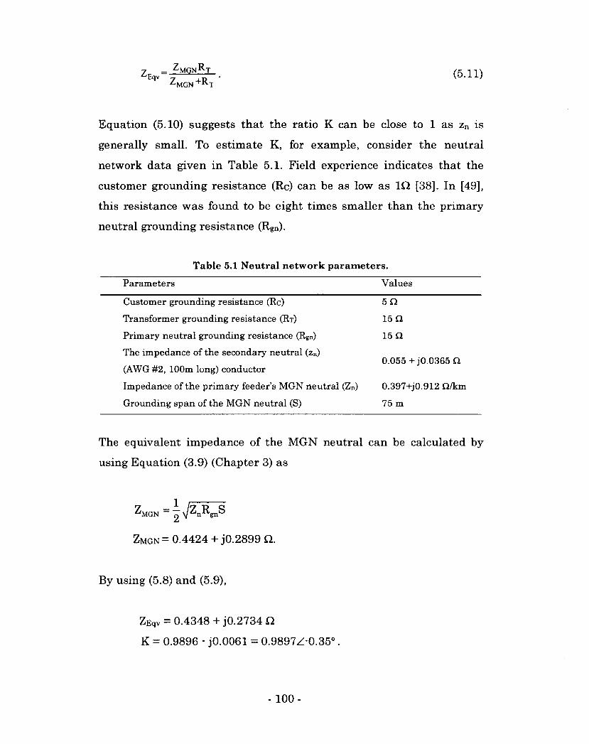
- Zmgn^T 7 xD ^MGN

(5.11)

Equation (5.10) suggests that the ratio K can be close to 1 as zn is

generally small. To estimate K, for example, consider the neutral

network data given in Table 5.1. Field experience indicates that the

customer grounding resistance (Rc) can be as low as 1Q [38], In [49],

this resistance was found to be eight times smaller than the primary

neutral grounding resistance (Rgn).

Table 5.1 Neutral network parameters.

Parameters Values

Customer grounding resistance (Rc) 5£2

Transformer grounding resistance (RT) 15 Q

Primary neutral grounding resistance (Rgn) 15 a

The impedance of the secondary neutral (zn) The impedance of the secondary neutral (zn) 0.055 + j0.0365 CI

(AWG#2, 100m long) conductor 0.055 + j0.0365 CI

Impedance of the primary feeder's MGN neutral (Zn) 0.397+j0.912 Q/km

Grounding span of the MGN neutral (S) 75 m

The equivalent impedance of the MGN neutral can be calculated by

using Equation (3.9) (Chapter 3) as

^MGN =

ZMGN = 0.4424 + j0.2899 Q.

By using (5.8) and (5.9),

ZEqv = 0.4348 + j0.2734 Q.

K = 0.9896 - j0.0061 = 0.9897Z-0.350.

- 100-

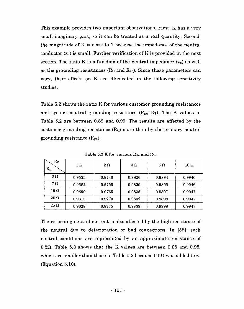
This example provides two important observations. First, K has a very

small imaginary part, so it can be treated as a real quantity. Second,

the magnitude of K is close to 1 because the impedance of the neutral

conductor (zn) is small. Further verification of K is provided in the next

section. The ratio K is a function of the neutral impedance (zn) as well

as the grounding resistances (Rc and Rgn). Since these parameters can

vary, their effects on K are illustrated in the following sensitivity

studies.

Table 5.2 shows the ratio K for various customer grounding resistances

and system neutral grounding resistance (Rgn=RT). The K values in

Table 5.2 are between 0.82 and 0.99. The results are affected by the

customer grounding resistance (Rc) more than by the primary neutral

grounding resistance (Rgn).

Table 5.2 K for various Rgn and Rc.

\ R c

Rgn 1 ft 2ft 3ft 5 ft 10 ft

3ft 0.9533 0.9746 0.9826 0.9894 0.9946

7 a 0.9562 0.9755 0.9830 0.9895 0.9946

15 n 0.9599 0.9765 0.9835 0.9897 0.9947

20 ft 0.9615 0.9770 0.9837 0.9898 0.9947

25 ft 0.9628 0.9775 0.9839 0.9898 0.9947

The returning neutral current is also affected by the high resistance of

the neutral due to deterioration or bad connections. In [58], such

neutral conditions are represented by an approximate resistance of

0.5Q. Table 5.3 shows that the K values are between 0.68 and 0.95,

which are smaller than those in Table 5.2 because 0.5Q was added to zn

(Equation 5.10).

- 101 -

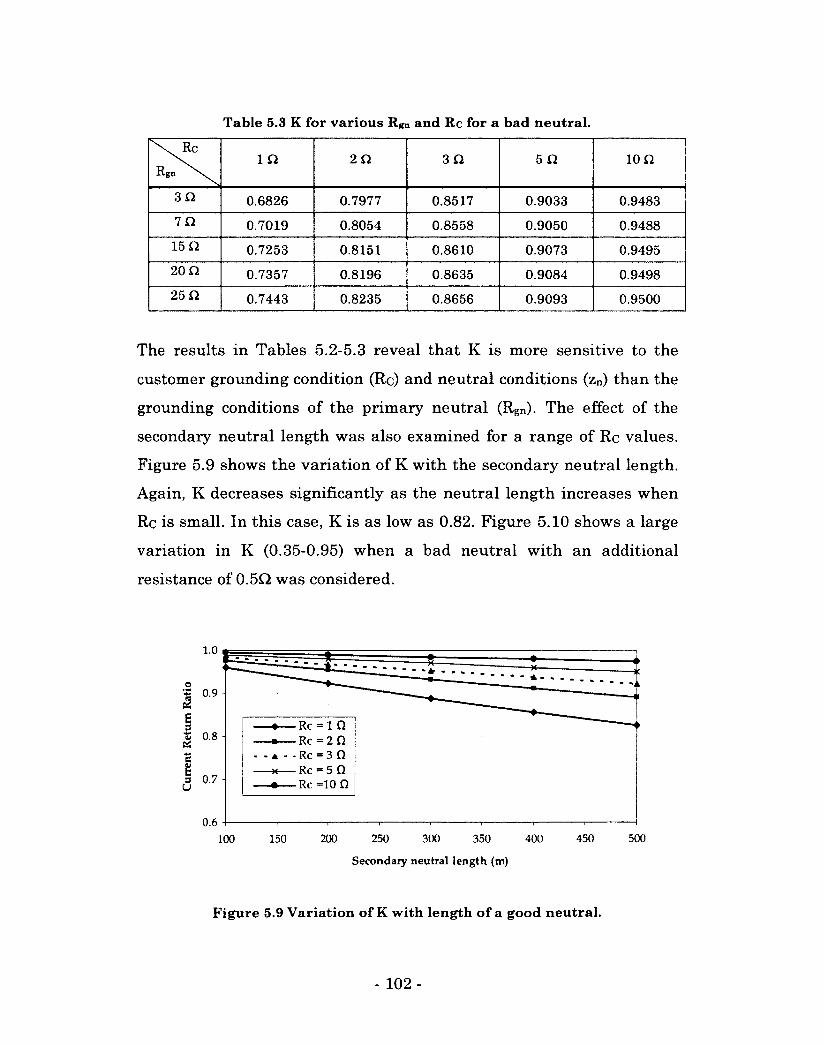
Table 5.3 K for various Rgn and Rc for a bad neutral.

\ R c

Rgn 1 n 2 Q 3 Q 5 n i o n

3Q 0.6826 0.7977 0.8517 0.9033 0.9483

1Q. 0.7019 0.8054 0.8558 0.9050 0.9488

15 n 0.7253 0.8151 0.8610 0.9073 0.9495

20 Q 0.7357 0.8196 0.8635 0.9084 0.9498

25 Q 0.7443 0.8235 0.8656 0.9093 0.9500

The results in Tables 5.2-5.3 reveal that K is more sensitive to the

customer grounding condition (Rc) and neutral conditions (zn) than the

grounding conditions of the primary neutral (Rgn). The effect of the

secondary neutral length was also examined for a range of Rc values.

Figure 5.9 shows the variation of K with the secondary neutral length.

Again, K decreases significantly as the neutral length increases when

Rc is small. In this case, K is as low as 0.82. Figure 5.10 shows a large

variation in K (0.35-0.95) when a bad neutral with an additional

resistance of 0.5Q was considered.

1.0

o 0.9

-Rc = 1 Q - Rc = 2 Q • Rc = 3 Q - Rc = 5 Q - Rc =10 Q

0.8

c t 3 0.7 u

0.6

450 200 250 300 350 400 500 150 100

Secondary neutral length (m)

Figure 5.9 Variation of K with length of a good neutral.

- 102 -

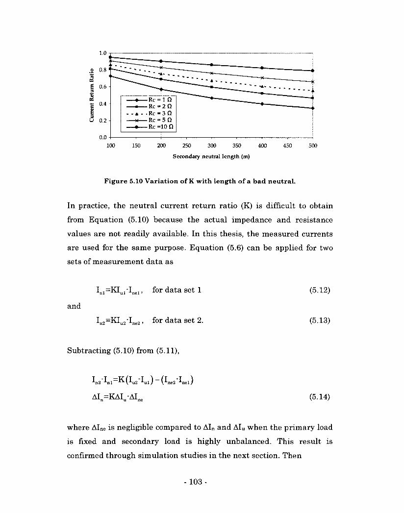
- - a - • Rc = 3 Q Rc = 5 Q

•— Rc =10 Q

100 150 200 250 300 350 400

Secondary neutral length (m)

450 500

Figure 5.10 Variation of K with length of a bad neutral.

In practice, the neutral current return ratio (K) is difficult to obtain

from Equation (5.10) because the actual impedance and resistance

values are not readily available. In this thesis, the measured currents

are used for the same purpose. Equation (5.6) can be applied for two

sets of measurement data as

Inl=KIul-Inel, for data set 1 (5.12)

and

In2=KIu2"Ine2 > for data Set 2- (5-13)

Subtracting (5.10) from (5.11),

^n2 ^nl—^(^2 ûl) (^ne2 ^nel)

Aln=KAlu-Alne (5.14)

where Alne is negligible compared to AIn and AIU when the primary load

is fixed and secondary load is highly unbalanced. This result is

confirmed through simulation studies in the next section. Then

- 103 -

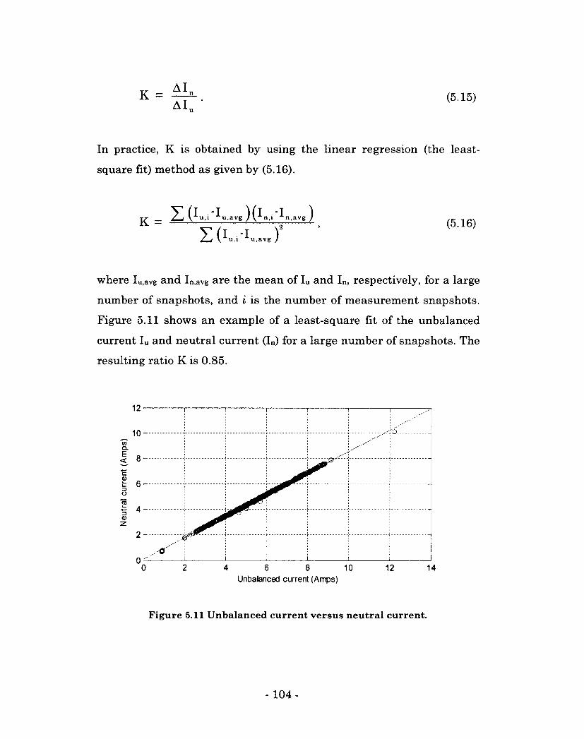
(5.15)

In practice, K is obtained by using the linear regression (the least-

square fit) method as given by (5.16).

where Iu,avg and In,avg are the mean of Iu and In, respectively, for a large

number of snapshots, and i is the number of measurement snapshots.

Figure 5.11 shows an example of a least-square fit of the unbalanced

current Iu and neutral current (In) for a large number of snapshots. The

resulting ratio K is 0.85.

(5.16)

12

10 c/> Q.

c a> 6

4

2

0 0 2 4 6 8 10

Unbalanced current (Amps) 12 14

Figure 5.11 Unbalanced current versus neutral current.

- 104-

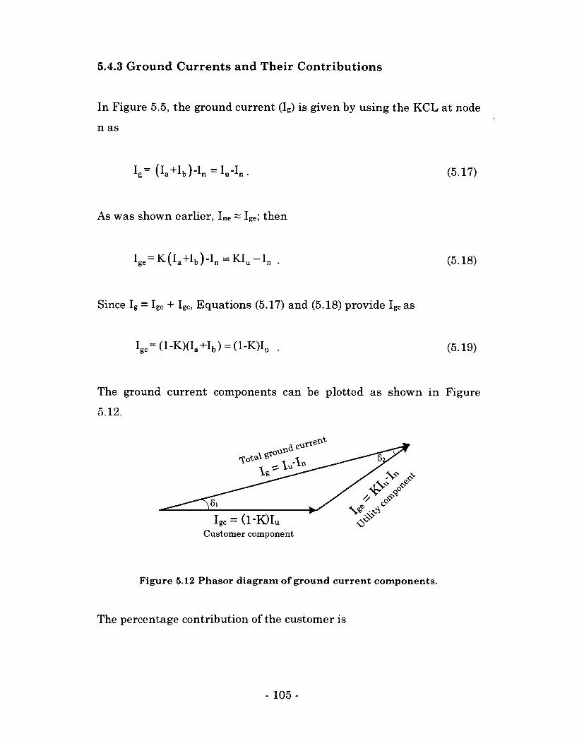
5.4.3 Ground Currents and Their Contributions

In Figure 5.5, the ground current (Ig) is given by using the KCL at node

n as

i.= (i,+ib)-i„=i„-in. (5.17)

As was shown earlier, Ine ~ Ige; then

I g e =K( l a +I b ) - I n =KI u - I„ . (5.18)

Since Ig = Ige + Igc, Equations (5.17) and (5.18) provide Igcas

Igc= (l-K)(Ia+Ib) = (1-K)IU . (5.19)

The ground current components can be plotted as shown in Figure

5.12.

V6

Igc = (l"K)lu

Customer component

Figure 5.12 Phasor diagram of ground current components.

The percentage contribution of the customer is

- 105

IIJcostf, | (l-K)I | F' =_i£ x 100% = —cos£, x 100%,

I I I I I - I I ' 6f ' 1 u n 1

(5.20)

and the percentage contribution of the utility is

11 I cos& F' = —e! * x 100% = cos£2 x 100%, (5.21) IIJ u n

where Fe and Fc are the percentage contributions of the primary

system or utility and the customer, respectively.

If K = 1 or Iu = 0, the Fc = 0 and Fe = 100%. These results mean that

when either all the customer load current returns through the neutral

or the customer loads are balanced, the utility is fully responsible for

the stray voltage. Similarly, K = 0 represents the case of a broken

secondary neutral so that In = 0. Then, Fe = 0 and Fc = 100%; i.e., the

customer is fully responsible for the stray voltage. In reality, 0<K<1

and Iu* 0. Therefore, both utility and customer contributions exist.

The contribution to the stray voltage will be same as that given by

(5.20) and (5.21) because the stray voltages at the neutral bus of the

customer service panel are simply obtained by multiplying the above

currents by the resistance Re-

Mathematically, the total stray voltage is Vng=IgRc ,

the stray voltage due to the customer is Vnc=IgcRc,

and the stray voltage due to the utility is Vne=IgeRc •

- 106-

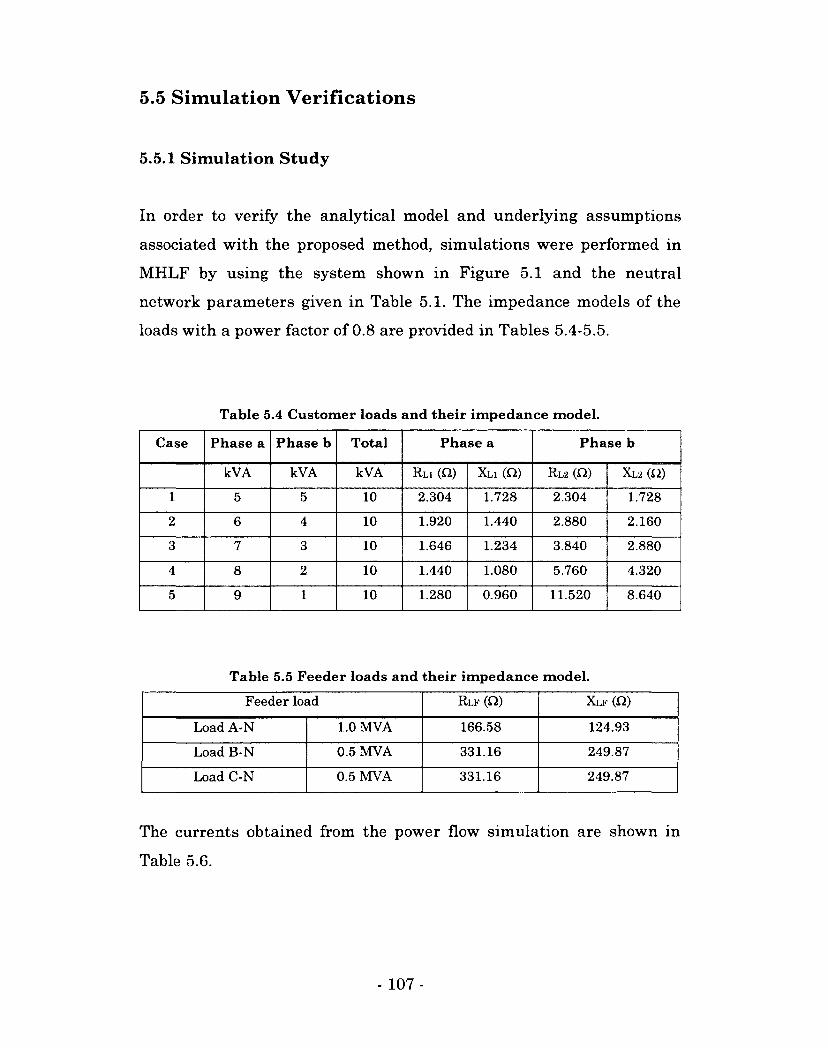
5.5 Simulation Verifications

5.5.1 Simulation Study

In order to verify the analytical model and underlying assumptions

associated with the proposed method, simulations were performed in

MHLF by using the system shown in Figure 5.1 and the neutral

network parameters given in Table 5.1. The impedance models of the

loads with a power factor of 0.8 are provided in Tables 5.4-5.5.

Table 5.4 Customer loads and their impedance model.

Case Phase a Phase b Total Phase a Phase b

kVA kVA kVA Ru (£2) XLI (ST2) Rl2 (£"2) XL2 («)

1 5 5 10 2.304 1.728 2.304 1.728

2 6 4 10 1.920 1.440 2.880 2.160

3 7 3 10 1.646 1.234 3.840 2.880

4 8 2 10 1.440 1.080 5.760 4.320

5 9 1 10 1.280 0.960 11.520 8.640

Table 5.5 Feeder loads and their impedance model.

Feeder load RLF (F2) XLF (P.)

Load A-N 1.0 MVA 166.58 124.93

Load B-N 0.5 MVA 331.16 249.87

Load C-N 0.5 MVA 331.16 249.87

The currents obtained from the power flow simulation are shown in

Table 5.6.

- 107 -

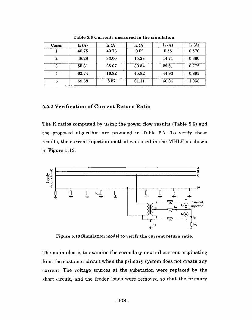
Table 5.6 Currents measured in the simulation.

Cases la (A) lb (A) lu (A) In (A) Ig (A)

1 40.75 40.73 0.02 0.55 0.576

2 48.28 33.00 15.28 14.71 0.660

3 55.61 25.07 30.54 29.81 0.772

4 62.74 16.92 45.82 44.93 0.895

5 69.68 8.57 61.11 60.06 1.058

5.5.2 Verification of Current Return Ratio

The K ratios computed by using the power flow results (Table 5.6) and

the proposed algorithm are provided in Table 5.7. To verify these

results, the current injection method was used in the MHLF as shown

in Figure 5.13.

CL -S

a t; C/> o

Current injection m

Figure 5.13 Simulation model to verify the current return ratio.

The main idea is to examine the secondary neutral current originating

from the customer circuit when the primary system does not create any

current. The voltage sources at the substation were replaced by the

short circuit, and the feeder loads were removed so that the primary

- 108-

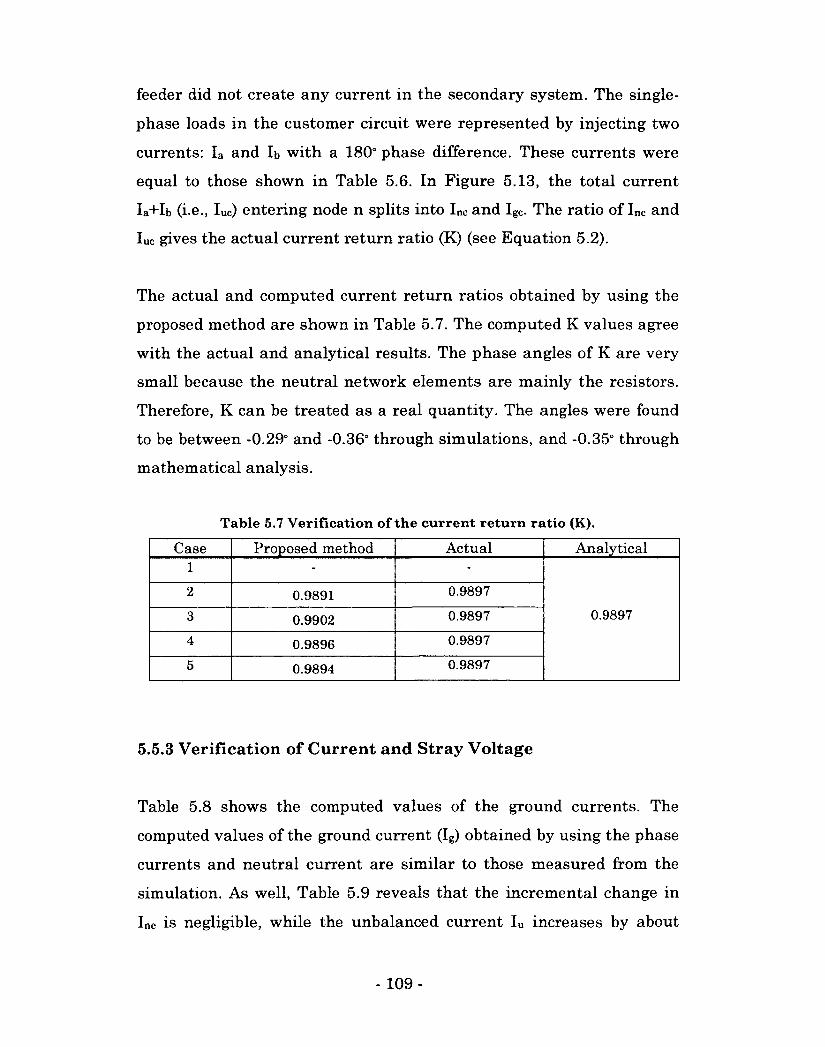
feeder did not create any current in the secondary system. The single-

phase loads in the customer circuit were represented by injecting two

currents: Ia and lb with a 180° phase difference. These currents were

equal to those shown in Table 5.6. In Figure 5.13, the total current

Ia+Ib (i e., Iuc) entering node n splits into Inc and Igc. The ratio of Inc and

Iuc gives the actual current return ratio (K) (see Equation 5.2).

The actual and computed current return ratios obtained by using the

proposed method are shown in Table 5.7. The computed K values agree

with the actual and analytical results. The phase angles of K are very

small because the neutral network elements are mainly the resistors.

Therefore, K can be treated as a real quantity. The angles were found

to be between -0.29° and -0.36° through simulations, and -0.35° through

mathematical analysis.

Table 5.7 Verification of the current return ratio (K).

Case Proposed method Actual Analytical 1 - -

2 0.9891 0.9897

3 0.9902 0.9897 0.9897

4 0.9896 0.9897

5 0.9894 0.9897

5.5.3 Verification of Current and Stray Voltage

Table 5.8 shows the computed values of the ground currents. The

computed values of the ground current (Ig) obtained by using the phase

currents and neutral current are similar to those measured from the

simulation. As well, Table 5.9 reveals that the incremental change in

Ine is negligible, while the unbalanced current Iu increases by about

- 109-

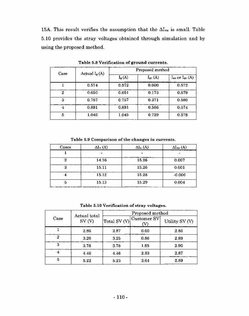
15A. This result verifies the assumption that the AIne is small. Table

5.10 provides the stray voltages obtained through simulation and by

using the proposed method.

Table 5.8 Verification of ground currents.

Case Actual Ig (A) Proposed method

Case Actual Ig (A) It (A) Igc (A) Ine Or Ige (A)

1 0.574 0.572 0.000 0.572

2 0.650 0.651 0.173 0.579

3 0.757 0.757 0.371 0.580

4 0.891 0.891 0.566 0.574

5 1.046 1.045 0.729 0.578

Table 5.9 Comparison of the changes in currents.

Cases AI„ (A) AIu (A) AIne (A)

1 - - -

2 14.16 15.26 0.007

3 15.11 15.26 0.001

4 15.12 15.28 -0.006

5 15.13 15.29 0.004

Table 5.10 Verification of stray voltages.

Case Actual total SV (V)

Proposed method Case Actual total

SV (V) Total SV (V) Customer SV (V) Utility SV (V)

1 2.86 2.87 0.00 2.86

2 3.26 3.25 0.86 2.89

3 3.78 3.78 1.85 2.90

4 4.46 4.46 2.83 2.87

5 5.22 5.23 3.64 2.89

- 110-

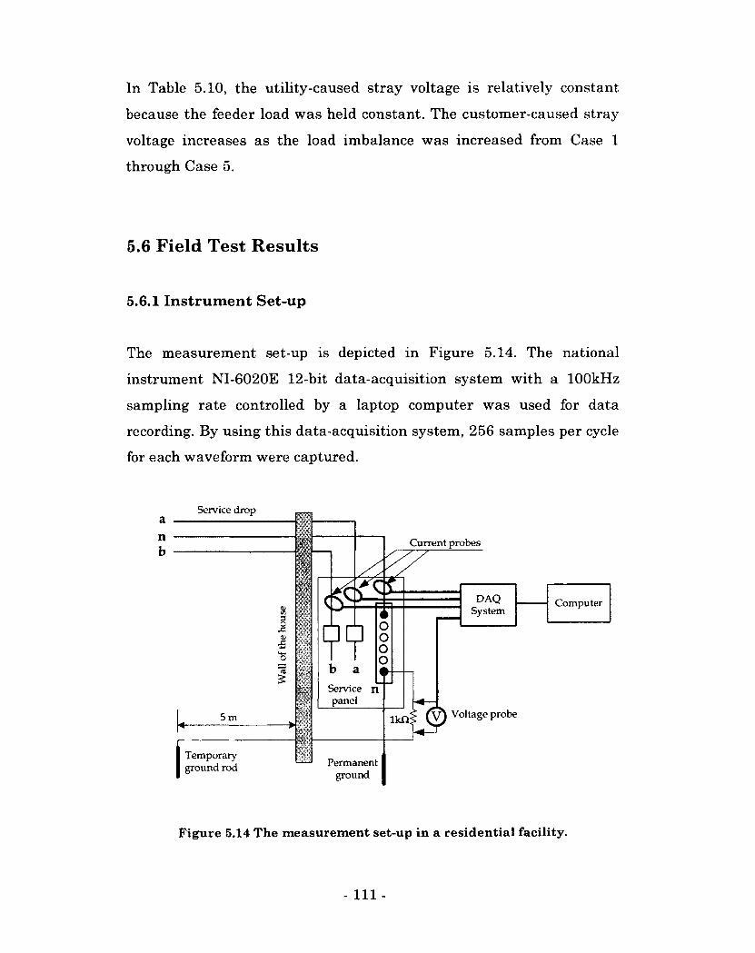
In Table 5.10, the utility-caused stray voltage is relatively constant

because the feeder load was held constant. The customer-caused stray

voltage increases as the load imbalance was increased from Case 1

through Case 5.

5.6 Field Test Results

5.6.1 Instrument Set-up

The measurement set-up is depicted in Figure 5.14. The national

instrument NI-6020E 12-bit data-acquisition system with a 100kHz

sampling rate controlled by a laptop computer was used for data

recording. By using this data-acquisition system, 256 samples per cycle

for each waveform were captured.

Service drop a n b

Current probes

DAQ System

Computer

S3

Service n panel

lkni fy) Voltage probe 5 m

Temporary ground rod Permanent

ground

Figure 5.14 The measurement set-up in a residential facility.

- Ill -

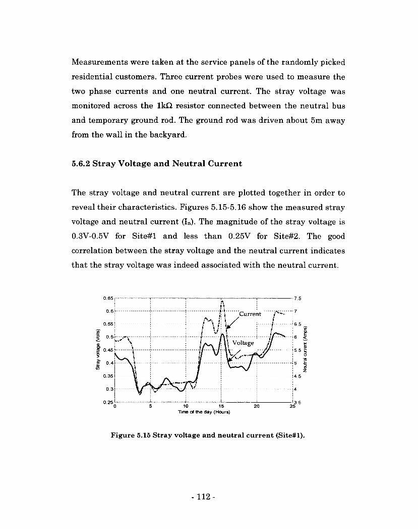
Measurements were taken at the service panels of the randomly picked

residential customers. Three current probes were used to measure the

two phase currents and one neutral current. The stray voltage was

monitored across the lkQ resistor connected between the neutral bus

and temporary ground rod. The ground rod was driven about 5m away

from the wall in the backyard.

5.6.2 Stray Voltage and Neutral Current

The stray voltage and neutral current are plotted together in order to

reveal their characteristics. Figures 5.15-5.16 show the measured stray

voltage and neutral current (In). The magnitude of the stray voltage is

0.3V-0.5V for Site#l and less than 0.25V for Site#2. The good

correlation between the stray voltage and the neutral current indicates

that the stray voltage was indeed associated with the neutral current.

0.65 7.5

Current

0.55 b 6.5

£ I

Voltage 0.45 h 5.5

0 35 4.5

0.3

0.25 3.5 10 15

Time o# the day (Hours) 20 25

Figure 5.15 Stray voltage and neutral current (Site#l).

- 112-

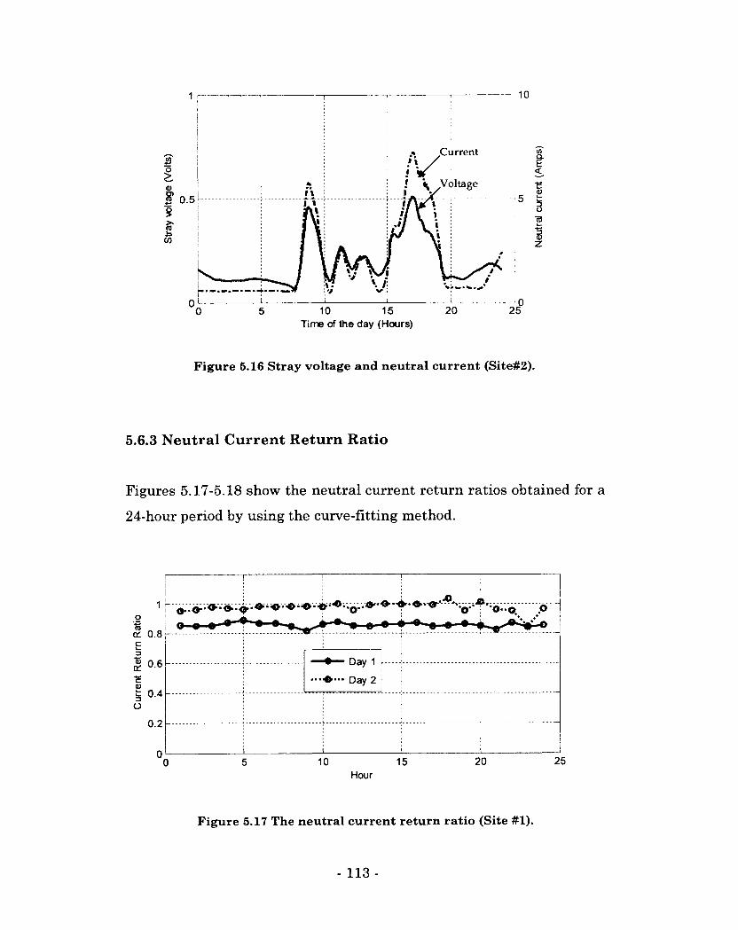
Current

Time of the day (Hours)

Figure 5.16 Stray voltage and neutral current (Site#2).

5.6.3 Neutral Current Return Ratio

Figures 5.17-5.18 show the neutral current return ratios obtained for a

24-hour period by using the curve-fitting method.

* Day 1

• •••©— Day 2

* Day 1

• •••©— Day 2

10 15 Hour

20 25

Figure 5.17 The neutral current return ratio (Site #1).

- 113 -

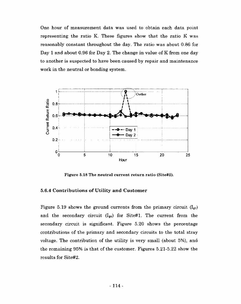
One hour of measurement data was used to obtain each data point

representing the ratio K. These figures show that the ratio K was

reasonably constant throughout the day. The ratio was about 0.86 for

Day 1 and about 0.96 for Day 2. The change in value of K from one day

to another is suspected to have been caused by repair and maintenance

work in the neutral or bonding system.

1

0 to 0.8 01 C

I 0.6 cc

t 0.4 3 o

0.2

0 0 5 10 15 20 25

Hour

Figure 5.18 The neutral current return ratio (Site#2).

5.6.4 Contributions of Utility and Customer

Figure 5.19 shows the ground currents from the primary circuit (Igc)

and the secondary circuit (Ige) for Site#l. The current from the

secondary circuit is significant. Figure 5.20 shows the percentage

contributions of the primary and secondary circuits to the total stray

voltage. The contribution of the utility is very small (about 5%), and

the remaining 95% is that of the customer. Figures 5.21-5.22 show the

results for Site#2.

T 7 M •-l \ • 1

Outlier

1 * J \

—<>•-• Day 1

O Day 2

- 114-

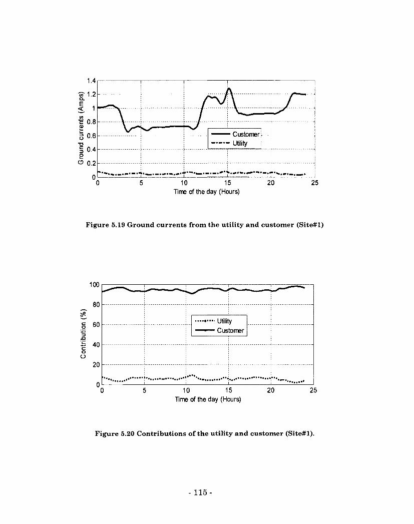
1.4

lo' 1.2 CL

I 1 •w* to c 0.8 ©

o T3 c 3 o

0.6

0.4

O 0.2

0

\ r \ / ^ / V

— Customer — Customer

10 15


20 25

Figure 5.19 Ground currents from the utility and customer (Site#l)

3 XI c o O

100

80

60

40

20

0

—•••• Utility

Customer

—•••• Utility

Customer

10 15


20 25

Figure 5.20 Contributions of the utility and customer (Site#l).

- 115-

• Customer

• Utility (/) Q.

CO * a> L—

3 o "S 3 s o

-0.5 20


Figure 5.21 Ground currents from the utility and customer (Site#2).

120

100

g. 80

1 60 3 .Q

'u. 40 1 o 20

0

-20

rW.-j"*'

Utility • Customer

/ *. A "'-f ; •»* • • • ••• • »

10 15 Time of the day (Hours)

20 25

Figure 5.22 Contributions of the utility and customer (Site#2).

The measured stray voltage and estimated ground currents are plotted

in Figure 5.23-5.24 for both sites. The ground current was obtained

from the neutral current and load currents, irrespective of the stray

voltage. These were found to be in good correlation with the stray

voltages. This result suggests that the method can effectively

reproduce the ground current.

- 116-

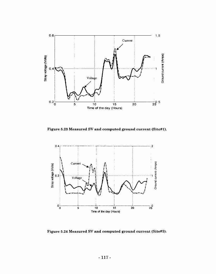
0.6

Current

Voltage

0.2 0.5 20 25


Figure 5.23 Measured SV and computed ground current (Site#l).

Current

Voltige


Figure 5.24 Measured SV and computed ground current (Site#2).

- 117 -

5.7 Application and Sensitivity Study

The potential applications of the proposed method were investigated

through sensitivity studies of various parameters such as the customer

grounding resistance, secondary neutral conductor impedance, primary

neutral grounding resistance, and broken primary neutral. In these

studies, a 2.0MVA unbalanced load (Table 5.5) was applied at the end

of the feeder, and a total load of lOkVA was connected (Phase-a: IkVA

and Phase-b: 9kVA) in the secondary system. As well, the application

of the method is discussed under operating conditions in which either

the customer load or the feeder load is acting alone.

5.7.1 Customer Grounding Conditions

The grounding resistance (Rc) was varied between 1Q and 15Q to

investigate its effect on the stray voltage. The primary neutral

grounding resistance was held constant at 15£2. As shown earlier, the

ratio K increases noticeably when Rc increases. Figures 5.25-5.26 show

the stray voltages and percentage contributions. The stray voltage

increases significantly as Rc increases. However, the percentage

contributions remain the same because both the customer and utility

components of the stray voltage increase proportionately. Based on

these results, the following conclusions can be made:

• The percentage contribution index is unable to respond to a

variation of Rc-

• A high Rc is the main suspect for the stray voltage problem if K

and the stray voltage increase, but the percentage contributions

remain stable. In other words, stray voltage monitoring can reveal

the grounding conditions.

- 118-

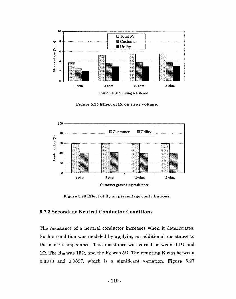
10

^ 8

0) bfi 2 w** o > ra £ c/5

1 ohm

E3 Total SV • Customer • Utility

5 ohm 10 ohm

Customer grounding resistance

15 ohm

Figure 5.25 Effect of Rc on stray voltage.

e _o s Xt '£ G O u

100

80

60 -

40 -

20 -

ED Customer E3 Utility

1 ohm 5 ohm 10 ohm

Customer grounding resistance

15 ohm

Figure 5.26 Effect of Rc on percentage contributions.

5.7.2 Secondary Neutral Conductor Conditions

The resistance of a neutral conductor increases when it deteriorates.

Such a condition was modeled by applying an additional resistance to

the neutral impedance. This resistance was varied between O.lil and

ID. The Rgn was 15Q, and the Rc was 5Q. The resulting K was between

0.8378 and 0.9897, which is a significant variation. Figure 5.27

- 119 -

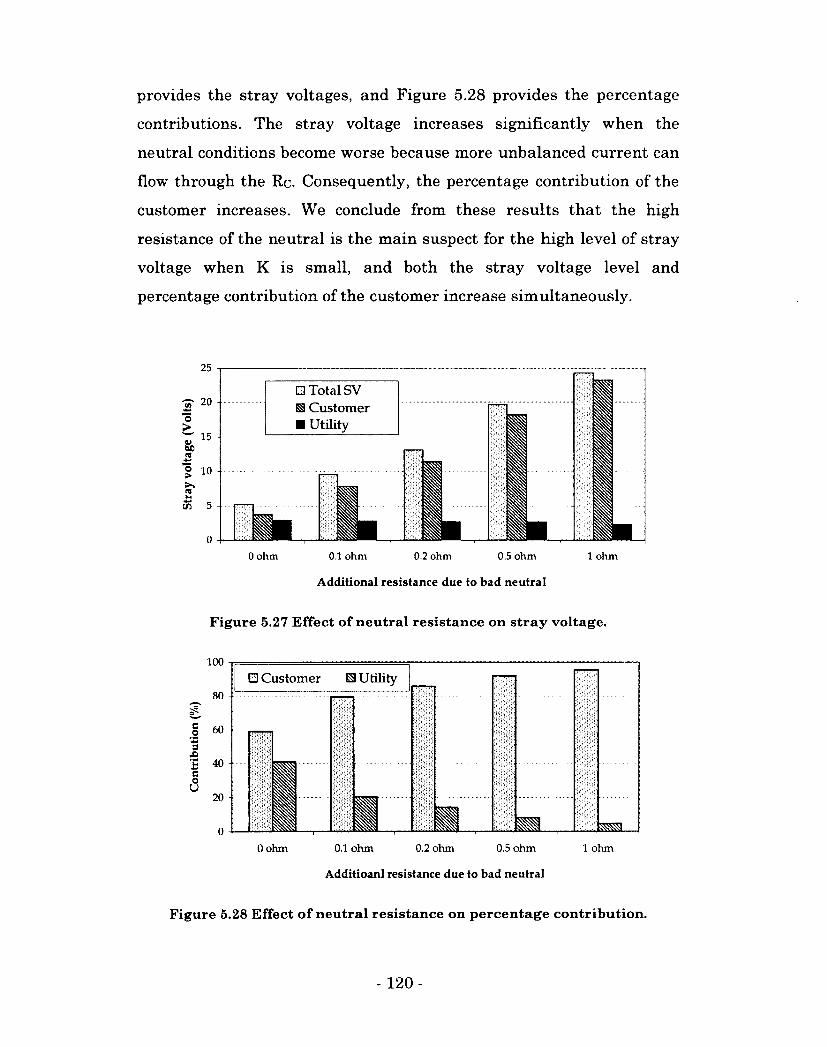
provides the stray voltages, and Figure 5.28 provides the percentage

contributions. The stray voltage increases significantly when the

neutral conditions become worse because more unbalanced current can

flow through the Rc. Consequently, the percentage contribution of the

customer increases. We conclude from these results that the high

resistance of the neutral is the main suspect for the high level of stray

voltage when K is small, and both the stray voltage level and

percentage contribution of the customer increase simultaneously.

25

• Total SV S3 Customer • Utility

0 ohm 0.1 ohm 0.2 ohm 0.5 ohm

Additional resistance due to bad neutral

1 ohm

Figure 5.27 Effect of neutral resistance on stray voltage.

100

80

60

40

20

0

c o •B 3 Xl £ C o U

E3 Customer ^ Utility

0 ohm 0.1 ohm 0.2 ohm 0.5 ohm

Additioanl resistance due to bad neutral

1 ohm

Figure 5.28 Effect of neutral resistance on percentage contribution.

- 120-

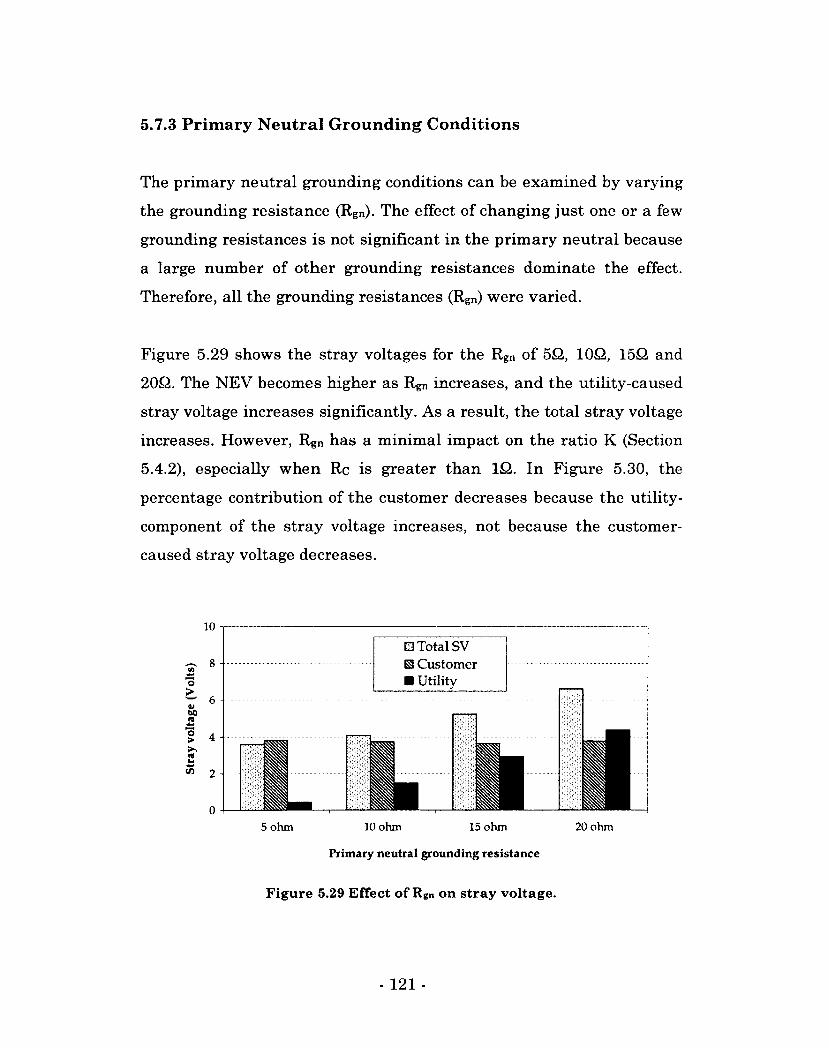
5.7.3 Primary Neutral Grounding Conditions

The primary neutral grounding conditions can be examined by varying

the grounding resistance (Rgn). The effect of changing just one or a few

grounding resistances is not significant in the primary neutral because

a large number of other grounding resistances dominate the effect.

Therefore, all the grounding resistances (Rgn) were varied.

Figure 5.29 shows the stray voltages for the Rgn of 5Q, 10£2, 15Q and

20Q. The NEV becomes higher as Rgn increases, and the utility-caused

stray voltage increases significantly. As a result, the total stray voltage

increases. However, Rgn has a minimal impact on the ratio K (Section

5.4.2), especially when Rc is greater than 1Q. In Figure 5.30, the

percentage contribution of the customer decreases because the utility-

component of the stray voltage increases, not because the customer-

caused stray voltage decreases.

10

o CO 8

• Total SV E3 Customer • Utility

5 ohm 10 ohm 15 ohm 20 ohm

Primary neutral grounding resistance

Figure 5.29 Effect of Rgn on stray voltage.

- 121 -

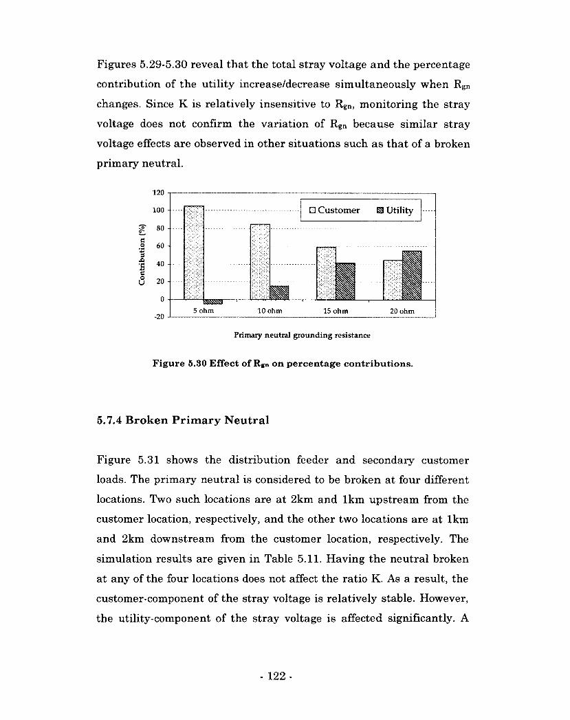
Figures 5.29-5.30 reveal that the total stray voltage and the percentage

contribution of the utility increase/decrease simultaneously when Rgn

changes. Since K is relatively insensitive to Rgn, monitoring the stray

voltage does not confirm the variation of Rgn because similar stray

voltage effects are observed in other situations such as that of a broken

primary neutral.

120

100

2 80

.2 60

I -<3 20

0

-20

Figure 5.30 Effect of Rgn on percentage contributions.

• Customer Utility

SSS5ST 5 ohm 10 ohm 15 ohm 20 ohm

Primary neutral grounding resistance

5.7.4 Broken Primary Neutral

Figure 5.31 shows the distribution feeder and secondary customer

loads. The primary neutral is considered to be broken at four different

locations. Two such locations are at 2km and 1km upstream from the

customer location, respectively, and the other two locations are at 1km

and 2km downstream from the customer location, respectively. The

simulation results are given in Table 5.11. Having the neutral broken

at any of the four locations does not affect the ratio K. As a result, the

customer-component of the stray voltage is relatively stable. However,

the utility-component of the stray voltage is affected significantly. A

- 122 -

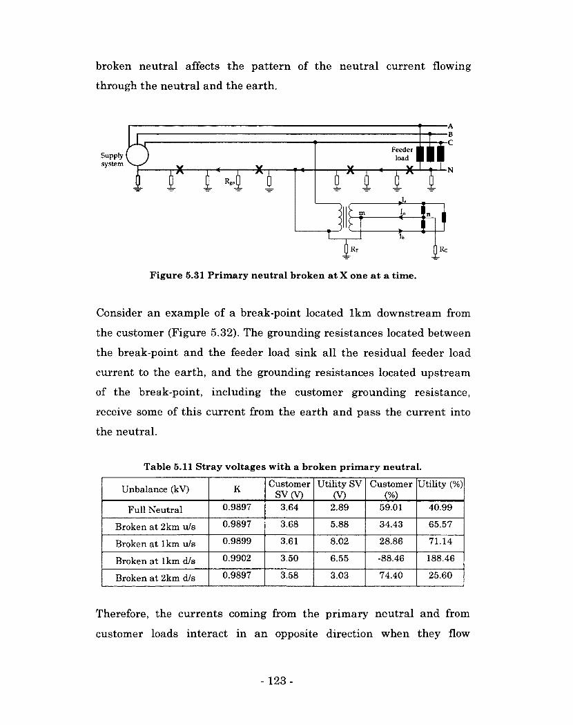
broken neutral affects the pattern of the neutral current flowing

through the neutral and the earth.

Feeder load Supply

system

m

Figure 5.31 Primary neutral broken at X one at a time.

Consider an example of a break-point located 1km downstream from

the customer (Figure 5.32). The grounding resistances located between

the break-point and the feeder load sink all the residual feeder load

current to the earth, and the grounding resistances located upstream

of the break-point, including the customer grounding resistance,

receive some of this current from the earth and pass the current into

the neutral.

Table 5.11 Stray voltages with a broken primary neutral.

Unbalance (kV) K Customer

SV(V) Utility SV

(V) Customer

(%) Utility (%)

Full Neutral 0.9897 3.64 2.89 59.01 40.99

Broken at 2km u/s 0.9897 3.68 5.88 34.43 65.57

Broken at 1km u/s 0.9899 3.61 8.02 28.86 71.14

Broken at 1km d/s 0.9902 3.50 6.55 -88.46 188.46

Broken at 2km d/s 0.9897 3.58 3.03 74.40 25.60

Therefore, the currents coming from the primary neutral and from

customer loads interact in an opposite direction when they flow

- 123 -

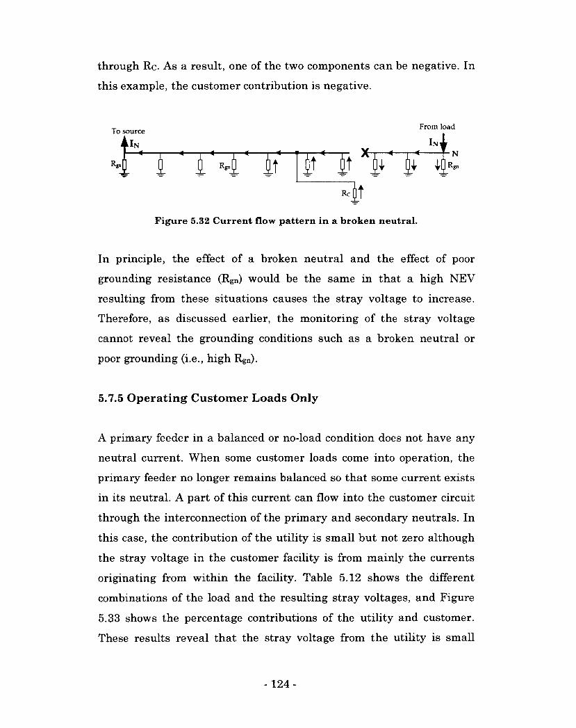
through Rc. As a result, one of the two components can be negative. In

this example, the customer contribution is negative.

i ' i ' 4 ' i f U t ' i t T T ~

From load

Figure 5.32 Current flow pattern in a broken neutral.

In principle, the effect of a broken neutral and the effect of poor

grounding resistance (Rgn) would be the same in that a high NEV

resulting from these situations causes the stray voltage to increase.

Therefore, as discussed earlier, the monitoring of the stray voltage

cannot reveal the grounding conditions such as a broken neutral or

poor grounding (i.e., high Rgn).

5.7.5 Operating Customer Loads Only

A primary feeder in a balanced or no-load condition does not have any

neutral current. When some customer loads come into operation, the

primary feeder no longer remains balanced so that some current exists

in its neutral. A part of this current can flow into the customer circuit

through the interconnection of the primary and secondary neutrals. In

this case, the contribution of the utility is small but not zero although

the stray voltage in the customer facility is from mainly the currents

originating from within the facility. Table 5.12 shows the different

combinations of the load and the resulting stray voltages, and Figure

5.33 shows the percentage contributions of the utility and customer.

These results reveal that the stray voltage from the utility is small

- 124-

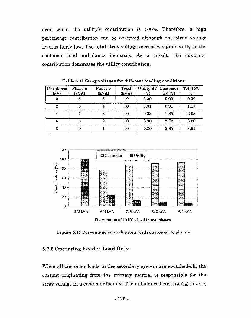
even when the utility's contribution is 100%. Therefore, a high

percentage contribution can be observed although the stray voltage

level is fairly low. The total stray voltage increases significantly as the

customer load unbalance increases. As a result, the customer

contribution dominates the utility contribution.

Table 5.12 Stray voltages for different loading conditions.

Unbalance (kV)

Phase a (kVA)

Phase b (kVA)

Total (kVA)

Utility SV (V)

Customer SV (V)

Total SV (V)

0 5 5 10 0.30 0.00 0.30

2 6 4 10 0.31 0.91 1.17

4 7 3 10 0.33 1.85 2.08

6 8 2 10 0.30 2.72 3.00

8 9 1 10 0.30 3.65 3.91

120

• Customer S Utility 100 -

2- 80 -c o 3 60 -XI

J3 e o U

40 -

20 -

6/4 kVA 5/5 kVA 7/3 kVA 8/2 kVA 9/1 kVA

Distribution of 10 kVA load in two phases

Figure 5.33 Percentage contributions with customer load only.

5.7.6 Operating Feeder Load Only

When all customer loads in the secondary system are switched-off, the

current originating from the primary neutral is responsible for the

stray voltage in a customer facility. The unbalanced current (Iu) is zero,

- 125 -

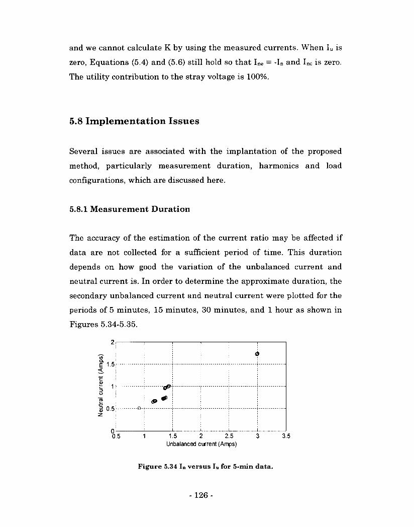
and we cannot calculate K by using the measured currents. When Iu is

zero, Equations (5.4) and (5.6) still hold so that Ine — -In and I nc is zero.

The utility contribution to the stray voltage is 100%.

5.8 Implementation Issues

Several issues are associated with the implantation of the proposed

method, particularly measurement duration, harmonics and load

configurations, which are discussed here.

5.8.1 Measurement Duration

The accuracy of the estimation of the current ratio may be affected if

data are not collected for a sufficient period of time. This duration

depends on how good the variation of the unbalanced current and

neutral current is. In order to determine the approximate duration, the

secondary unbalanced current and neutral current were plotted for the

periods of 5 minutes, 15 minutes, 30 minutes, and 1 hour as shown in

Figures 5.34-5.35.

2

wT Q. . _ E 1.5 <

11 0

"ro 1 0.5 z

0 0.5 1 1.5 2 2.5 3 3.5

Unbalanced current (Amps)

Figure 5.34 In versus Iu for 5-min data.

£ •

,

- 1 2 6 -

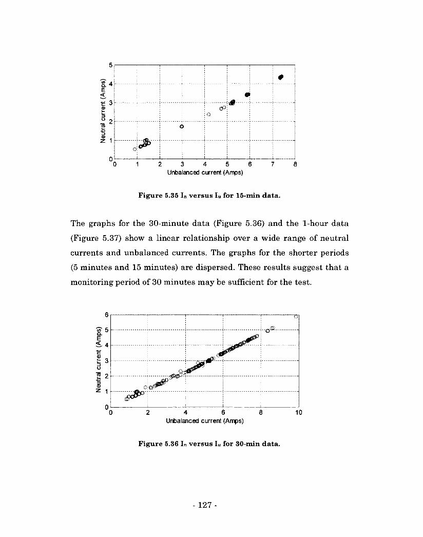
Q. t E <

« 3 <D l_ k_ 3 O o

3 0)

0

9 a

CP 0

CP

o

o «•>

0 1 2 3 4 5 6 7 8 Unbalanced current (Amps)


The graphs for the 30-minute data (Figure 5.36) and the 1-hour data

(Figure 5.37) show a linear relationship over a wide range of neutral

currents and unbalanced currents. The graphs for the shorter periods

(5 minutes and 15 minutes) are dispersed. These results suggest that a

monitoring period of 30 minutes may be sufficient for the test.

"3" 5 Q. E <4 -£ 0) i= 3 3 (J

2 2 3 0) 2 1

0 4 6

Unbalanced current (Amps) 10


- 127 -

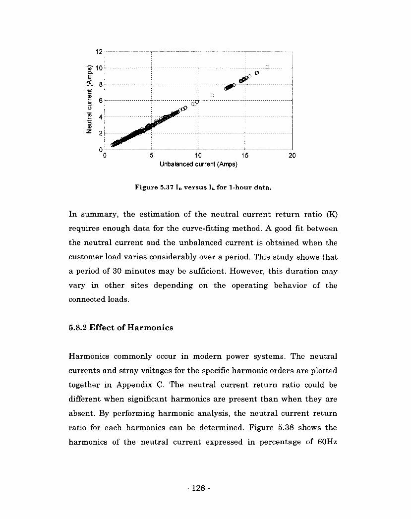
12

"5T 10 E

O

& c a> o 6 -

0 0 5 10 15 20

Unbalanced current (Amps)

Figure 5.37 In versus Iu for 1-hour data.

In summary, the estimation of the neutral current return ratio (K)

requires enough data for the curve-fitting method. A good fit between

the neutral current and the unbalanced current is obtained when the

customer load varies considerably over a period. This study shows that

a period of 30 minutes may be sufficient. However, this duration may

vary in other sites depending on the operating behavior of the

connected loads.

5.8.2 Effect of Harmonics

Harmonics commonly occur in modern power systems. The neutral

currents and stray voltages for the specific harmonic orders are plotted

together in Appendix C. The neutral current return ratio could be

different when significant harmonics are present than when they are

absent. By performing harmonic analysis, the neutral current return

ratio for each harmonics can be determined. Figure 5.38 shows the

harmonics of the neutral current expressed in percentage of 60Hz

- 128-

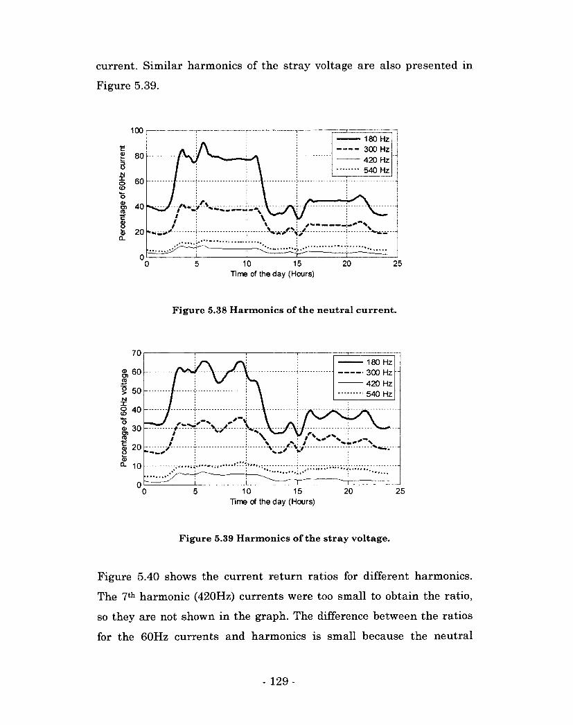
current. Similar harmonics of the stray voltage are also presented in

Figure 5.39.

100 180 Hz

— 300 Hz 420 Hz

•• • 540 Hz

80

CO

O) 40

20


Figure 5.38 Harmonics of the neutral current.

70 — 180 Hz — 300 Hz — 420 Hz

540 Hz 50

£ 40

w <u 30 cn

10


Figure 5.39 Harmonics of the stray voltage.

Figure 5.40 shows the current return ratios for different harmonics.

The 7th harmonic (420Hz) currents were too small to obtain the ratio,

so they are not shown in the graph. The difference between the ratios

for the 60Hz currents and harmonics is small because the neutral

- 129-

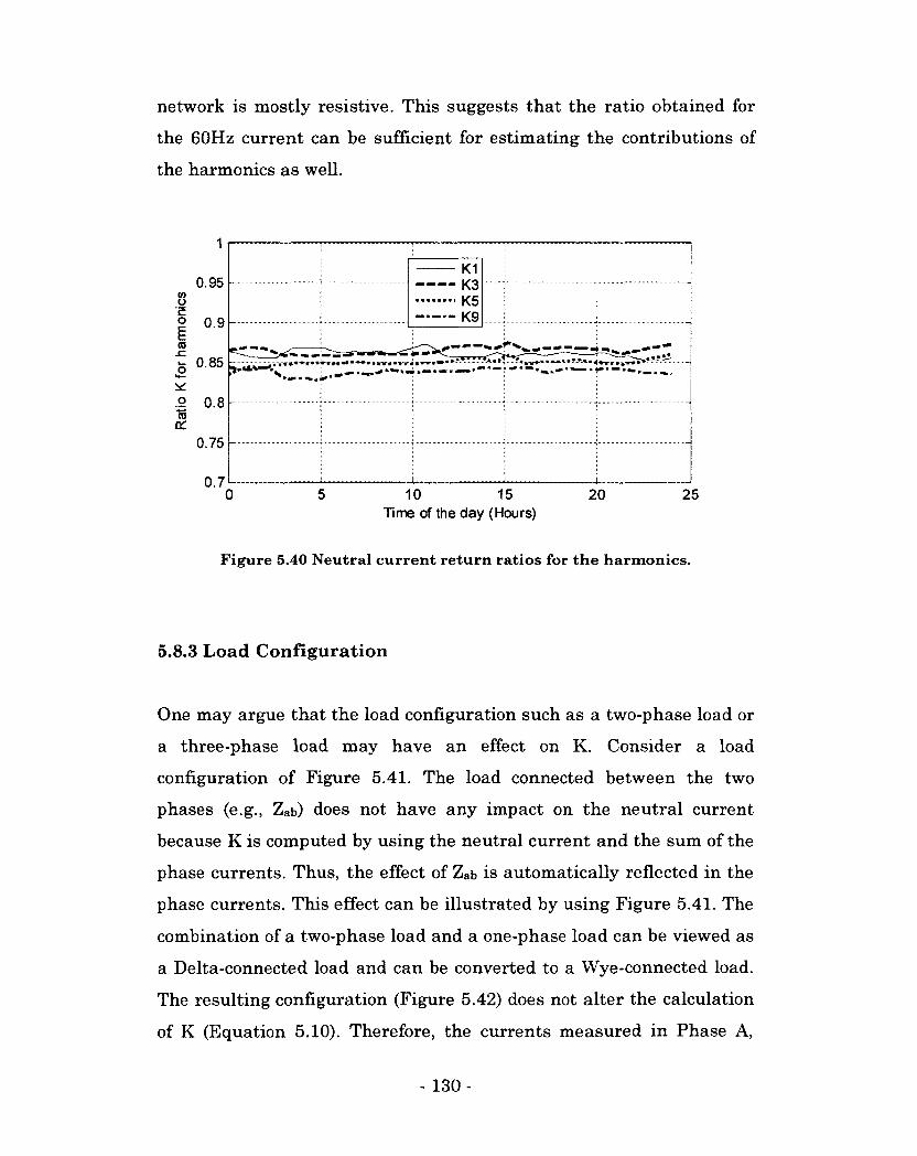
network is mostly resistive. This suggests that the ratio obtained for

the 60Hz current can be sufficient for estimating the contributions of

the harmonics as well.

0.95

- 0.85

0.75

0.7

- K3 K5

- K9

' I L i I I

0 5 10 15 20 25 Time of the day (Hours)

Figure 5.40 Neutral current return ratios for the harmonics.

5.8.3 Load Configuration

One may argue that the load configuration such as a two-phase load or

a three-phase load may have an effect on K. Consider a load

configuration of Figure 5.41. The load connected between the two

phases (e.g., Zab) does not have any impact on the neutral current

because K is computed by using the neutral current and the sum of the

phase currents. Thus, the effect of Zab is automatically reflected in the

phase currents. This effect can be illustrated by using Figure 5.41. The

combination of a two-phase load and a one-phase load can be viewed as

a Delta-connected load and can be converted to a Wye-connected load.

The resulting configuration (Figure 5.42) does not alter the calculation

of K (Equation 5.10). Therefore, the currents measured in Phase A,

- 130-

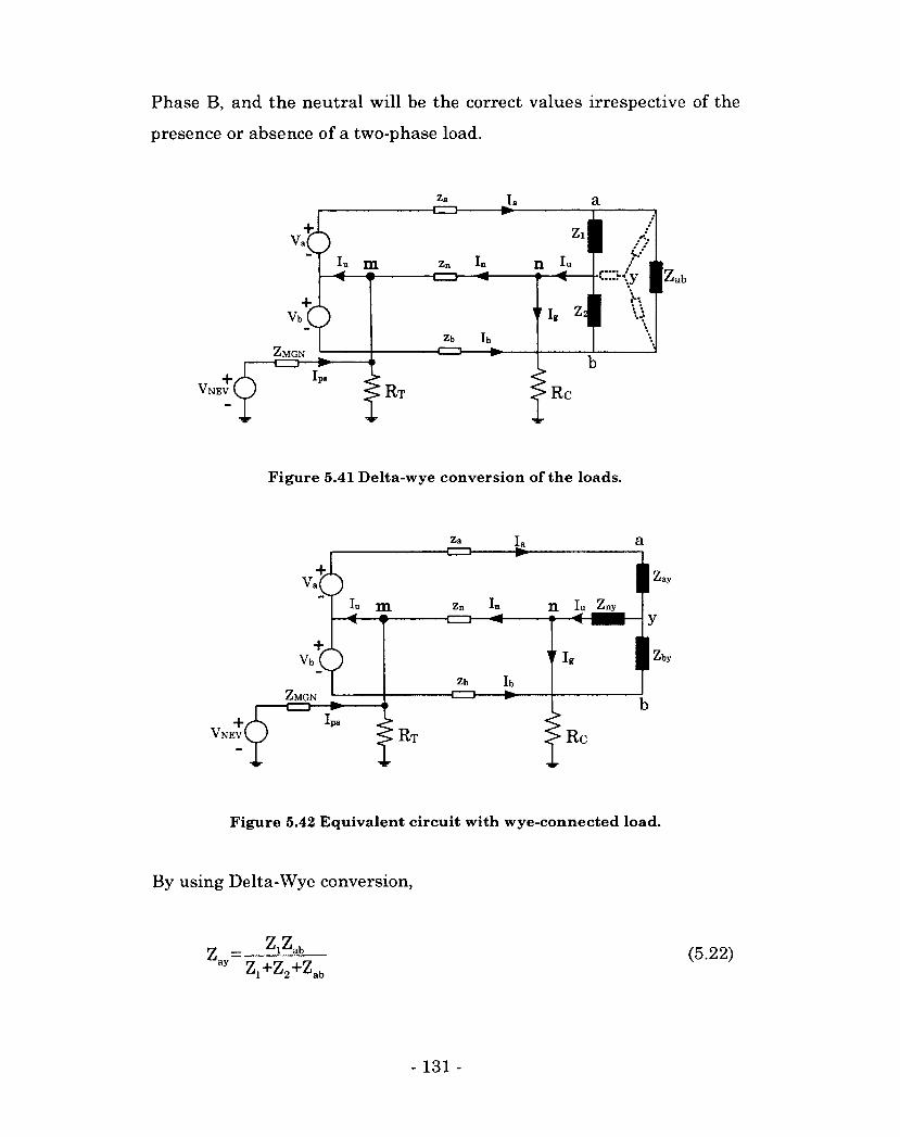
Phase B, and the neutral will be the correct values irrespective of the

presence or absence of a two-phase load.

ZMGN

VNEV Rc

Figure 5.41 Delta-wye conversion of the loads.

"ay

Zn

CZD-my

ZMGN

VNEV Rc

Figure 5.42 Equivalent circuit with wye-connected load.

By using Delta-Wye conversion,

Z = — — ( 5 2 2 ) ay Zj+Z2+Zab

- 131 -

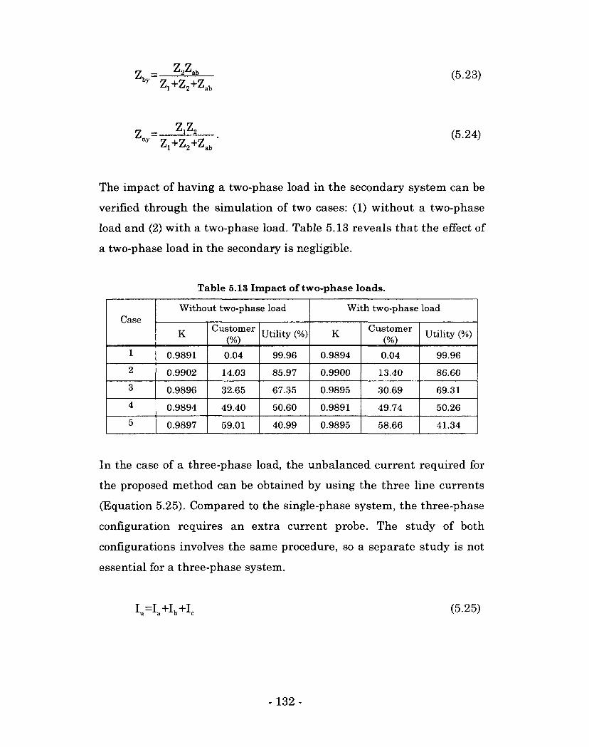
J b y ~

Z2Zab Zj+Z2+Z ab

(5.23)

ZIZ2 Zl+Z2+Z

ab

zny=„ ^ • (5-24)

The impact of having a two-phase load in the secondary system can be

verified through the simulation of two cases: (1) without a two-phase

load and (2) with a two-phase load. Table 5.13 reveals that the effect of

a two-phase load in the secondary is negligible.

Table 5.13 Impact of two-phase loads.

Case Without two-phase load With two-phase load

Case

K Customer

(%) Utility (%) K

Customer (%)

Utility (%)

1 0.9891 0.04 99.96 0.9894 0.04 99.96

2 0.9902 14.03 85.97 0.9900 13.40 86.60

3 0.9896 32.65 67.35 0.9895 30.69 69.31

4 0.9894 49.40 50.60 0.9891 49.74 50.26

5 0.9897 59.01 40.99 0.9895 58.66 41.34

In the case of a three-phase load, the unbalanced current required for

the proposed method can be obtained by using the three line currents

(Equation 5.25). Compared to the single-phase system, the three-phase

configuration requires an extra current probe. The study of both

configurations involves the same procedure, so a separate study is not

essential for a three-phase system.

Iu=Ia+Ib+Ic (5.25)

- 132 -

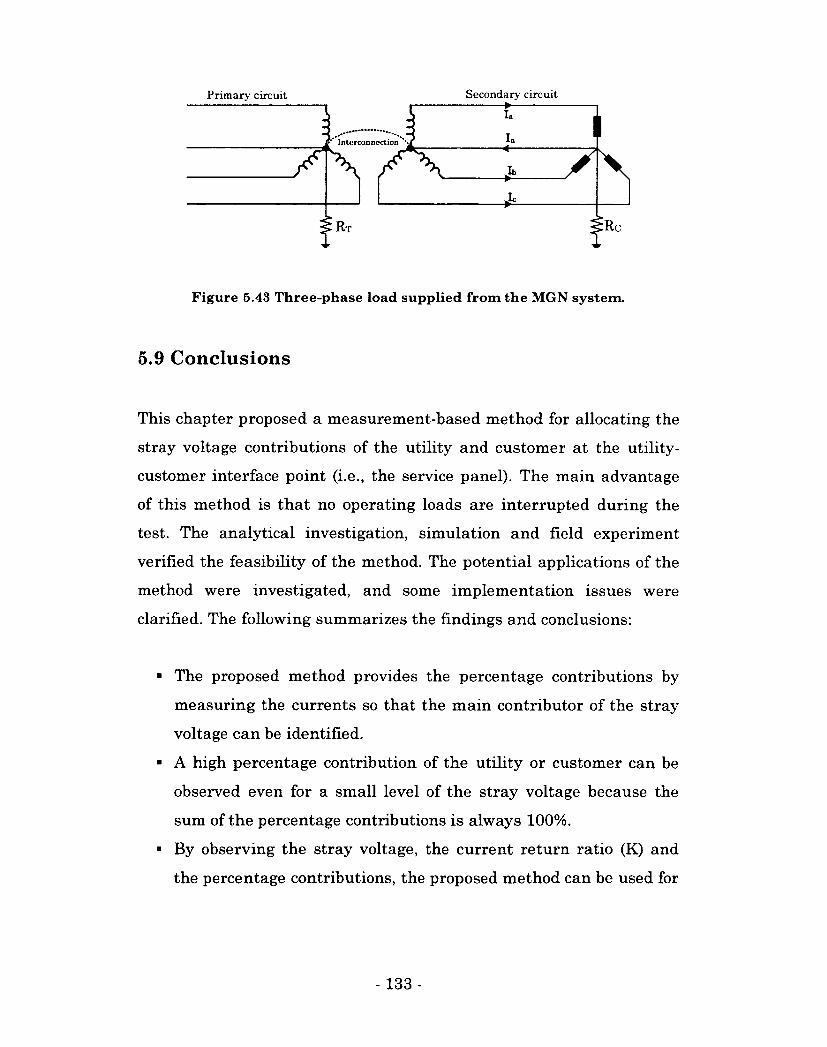
Primary circuit

Interconnection '

Secondary circuit •

la 1 y\ :Rc

Figure 5.43 Three-phase load supplied from the MGN system.

5.9 Conclusions

This chapter proposed a measurement-based method for allocating the

stray voltage contributions of the utility and customer at the utility-

customer interface point (i.e., the service panel). The main advantage

of this method is that no operating loads are interrupted during the

test. The analytical investigation, simulation and field experiment

verified the feasibility of the method. The potential applications of the

method were investigated, and some implementation issues were

clarified. The following summarizes the findings and conclusions:

• The proposed method provides the percentage contributions by

measuring the currents so that the main contributor of the stray

voltage can be identified.

• A high percentage contribution of the utility or customer can be

observed even for a small level of the stray voltage because the

sum of the percentage contributions is always 100%.

• By observing the stray voltage, the current return ratio (K) and

the percentage contributions, the proposed method can be used for

- 133 -

trouble-shooting the stray voltage problem and monitoring the

customer grounding and secondary neutral conditions.

• The ratio K changes significantly due to the variation of customer

grounding resistance and bad neutral conditions, but it does not

vary noticeably due to the grounding conditions of the primary

neutral.

• The field test results indicated that the data should be recorded

for about 30 minutes or more to obtain the ratio K by using a

curve-fitting method.

The stray voltage contribution determination method established in

this research is equally valid for a three-phase secondary system

although this method was developed by focusing on a single-phase

secondary system.

- 134-

6. Conclusions and Recommendations

6.1 Conclusions

The multi-grounded neutral (MGN) distribution systems are the most

common power delivery configurations in North America. The presence

of a neutral conductor and grounding arrangement makes these

systems' performances difficult to understand and assess. The existing

techniques to evaluate system performance are either not applicable to

MGN configurations or not able to provide a full understanding of the

electrical phenomena associated with operational problems. The main

objectives of this thesis were to develop an analytical understanding of

the electric characteristics of the MGN system, with the phenomena of

ground potential rise (GPR), temporary overvoltage (TOV) and stray

voltage as the main focus. Based on the analytical results obtained in

this research, the MGN parameters that play important roles were

identified, and some of the complex phenomena were clarified. These

findings were applied to establish a novel concept for determining the

contributions of off-site sources (e.g., the utility) and on-site sources

(e.g., the customer load) to the stray voltage level at the utility-

customer interface point.

The mechanism of GPR generation in MGN systems was illustrated,

and an analytical method was developed to assess the maximum GPR.

This method is capable of quantifying the impact of various MGN

- 135 -

parameters such as the grounding resistance, the neutral conductor

size and the grounding interval. The good agreement between the

analytical and simulation results demonstrated the accuracy of the

approximate methods. The following conclusions can be made from the

GPR studies:

• The voltage induced by the fault current through the coupling

with neutral conductor is the main cause of GPR in the case of

LG faults.

• The fault current is the most decisive factor for the magnitude of

the maximum GPR.

• The GPR is proportional to the equivalent impedance of the

MGN and the square-root of the grounding resistance, the

impedance of the neutral conductor, and the grounding interval.

• The maximum GPR occurs at the grounded node where the

induced shunt current source is located.

• The induced current sources are located at the ends of the

section of the neutral length exposed to the fault current.

One of the challenges with MGN systems is identifying the impacts of

the neutral current, which varies from segment to segment along the

neutral wire. A new "total neutral current" approach was proposed to

incorporate the effect of these currents in the TOV assessment. The

analytical equations developed for GPR calculation were employed to

further establish the TOV equations. The proposed method identifies

the various contributing factors such as the fault current and neutral

current, and quantifies their contributions to the TOV. The

effectiveness of the developed methods was verified through simulation

studies. From these studies, the following conclusions can be drawn:

- 136-

• The voltages induced by the fault current and the neutral

current are the most decisive factors for the TOV. While the

fault current caused about 30% to the TOV, the neutral current

compensated by about 10%. Therefore, the neutral currents

should be included in the overvoltage calculation.

• The substation neutral voltage, which contributed less than 2%,

is insignificant.

• The grounding parameters such as the grounding resistance and

grounding interval also have a small impact on the TOV.

A novel concept was conceived for allocating the stray voltage

contributions of the utility and the customer at the utility-customer

interface point, and a measurement-based method was established.

This method eliminates various practical difficulties associated with

the field test. For example, the operating loads are not interrupted,

and the portable loads are not required. The effectiveness of the

method was verified through analytical studies, simulations and field

experiments. A number of implementation issues, such as the duration

of the test, the harmonics and the load configurations, were clarified.

The main findings and conclusions are summarized as follows:

• The percentage contributions of the utility and customer can be

estimated effectively by measuring the currents only, and the

main contributor of the stray voltage can be identified.

• A high percentage contribution of the utility or customer can be

observed even for a small level of the stray voltage because the

sum of the percentage contributions is always 100%.

• The neutral-current return ratio (K) changes significantly due to

the variation of the customer grounding resistance and bad

neutral conditions, but does not vary noticeably with a change in

the grounding conditions of the primary neutral.

- 137 -

• The field test results suggest that recording data for 30 minutes

or more is sufficient to obtain the ratio K by using the curve-

fitting method.

• The effect of harmonics on the ratio K was minimal because this

ratio deals with neutral network which is mostly resistive.

The approximate formulae developed in this thesis to evaluate the

GPR of the MGN neutral can be used as a handy tool to evaluate the

GPR in many other applications, including the shield wire of the

transmission system, the neutral wire of the distribution system, and

the telephone cable. The findings of the TOV analysis are important for

the selection of surge arresters and insulation coordination. The

concept of the total neutral current approach in the TOV calculation

method together with the GPR analysis technique can be applied to

estimate the voltages created by the power line currents in nearby

conductors such as telephone cables, pipelines, and other power lines.

Similarly, the method established for distinguishing the stray voltage

sources can be used for the trouble-shooting of a stray voltage problem

by locating the main cause. As well, this method has the potential to be

applied in modern metering devices to monitor the customer grounding

and neutral conditions. The findings of the stray voltage studies also

provide an opportunity to explore stray voltage problems and

mitigation methods.

6.2 Recommendations for Future Work

6.2.1 Estimating the GPR along the Neutral Length

The magnitude and location of the highest GPR were identified in this

thesis. This result provides an opportunity to explore the technique to

- 138 -

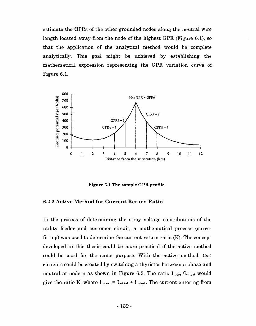
estimate the GPRs of the other grounded nodes along the neutral wire

length located away from the node of the highest GPR (Figure 6.1), so

that the application of the analytical method would be complete

analytically. This goal might be achieved by establishing the

mathematical expression representing the GPR variation curve of

Figure 6.1.

800 -r-

Max GPR = GPR6 700

^ 600 -v (O 'C 500 - GPR7-?

« 400 -- GPR5 = ?

300 - GPR4 = ? GPR8 = ?

100 -

0 1 2 3 4 5 6 7 8 9 1 0 1 1 1 2 Distance from the substation (km)

Figure 6.1 The sample GPR profile.

6.2.2 Active Method for Current Return Ratio

In the process of determining the stray voltage contributions of the

utility feeder and customer circuit, a mathematical process (curve-

fitting) was used to determine the current return ratio (K). The concept

developed in this thesis could be more practical if the active method

could be used for the same purpose. With the active method, test

currents could be created by switching a thyristor between a phase and

neutral at node n as shown in Figure 6.2. The ratio In-test/Iu-test would

give the ratio K, where Iu-test = la test + lb-test. The current entering from

- 139-

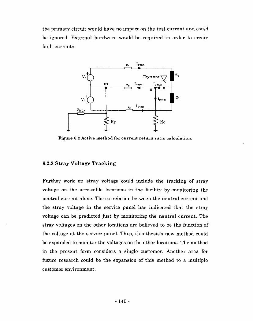
the primary circuit would have no impact on the test current and could

be ignored. External hardware would be required in order to create

fault currents.

Figure 6.2 Active method for current return ratio calculation.

6.2.3 Stray Voltage Tracking

Further work on stray voltage could include the tracking of stray

voltage on the accessible locations in the facility by monitoring the

neutral current alone. The correlation between the neutral current and

the stray voltage in the service panel has indicated that the stray

voltage can be predicted just by monitoring the neutral current. The

stray voltages on the other locations are believed to be the function of

the voltage at the service panel. Thus, this thesis's new method could

be expanded to monitor the voltages on the other locations. The method

in the present form considers a single customer. Another area for

future research could be the expansion of this method to a multiple

customer environment.

ZM

Thyristor

- 140 -

References

[1] ANSI/IEEE C2 — 2002, The National Electrical Safety Code®,

Section 09, IEEE Inc, 1995.

[2] R. Rudenberg, Transient Performance of Electric Power Systems,

New York: McGraw-Hill, 1950.

[3] A. P. Meliopoulos, "Impact of Grounding System Design on Power

Quality", IEEE Power Engineering Review, Nov 2001, p. 3-7.

[4] A. P. Meliopoulos, G. J. Cokkinides, K. R. Chakravarthi, "Effects

of Grounding on Distribution System Harmonic Resonance

Conditions", IEEE Transactions on Power Delivery, Vol. 4, No. 1,

January 1989, p. 475-682.

[5] IEEE C62.92.4-1991, Guide for the Application of Neutral

Grounding in Electrical Utility Systems, Part IV-Distribution,

1992.

[6] J. Burke, M. Marshal, "Distribution System Neutral Grounding,"

IEEE Proceedings of Transmission and Distribution Conference

and Exposition, Vol. 1, 2001, p. 166-170.

[7] IEEE Working Group, Voltages at Publicly and Privately

Accessible Locations, Trial Use Guide (Draft), 2009.

[8] D. W. Zipse, "Electrical Shock Hazard due to Stray Current (The

Shocking Shower) ", IEEE Industrial and Commercial Power

Systems Conference Record, 1999, p. 1-6.

[9] IEEE Std. 1159, Recommended Practice for Monitoring Electric

Power Quality, 1995.

[10] R. C. Dugan, M. F. McGranaghan, H. W. Beaty, Electrical Power

Systems Quality, McGraw-Hill Publishing, 1996.

- 141 -

[11] CIGRE WG 33.10 and IEEE Task Force on TOV, "Temporary

Overvoltages: Causes, Effects and Evaluation — Summary", IEEE

Power Engineering Review, Vol. 10, No. 6, p. 14-15.

[12] J. Acharya, W. Xu, "Voltage Swell Characteristics in Multi-

grounded Systems," IEEE Transactions on Power Delivery, Vol.

22, No. 2, April 2007, p. 1259-1260.

[13] J. Acharya, W. Xu, "Characteristics of Voltage Imbalance and

Neutral Current and Voltage Distributions in Multi-grounded

Systems," Journal of Power Energy and Systems, Vol. 29, No. 3,

2009, p. 193-199.

[14] J. Acharya, W. Xu, "Temporary Overvoltage and GPR

Characteristics of Distribution Feeders with Multi-grounded

Neutral", IEEE Transactions on Power Delivery, Vol. 25, No. 2,

April 2010, p. 1036-1044.

[15] J. Acharya, W. Xu, "Ground Potential Rise of Multi-grounded

Neutral and Shield Wires in Joint Systems", Electric Power

Systems Research, Vol. 80, April 2010, p. 1074-1081.

[16] Y. Wang, J. Acharya, W. Xu, "Shielding Effect of Multi-grounded

Neutral Wire on Power Line Induced Voltages", European

Transactions on Electric Power, Accepted, April 2010, 8p.

[17] A. P. Meliopoulos, Power System Grounding and Transients,

Marcel Dekker Inc., 1988.

[18] IEEE Std. 142-1991, Recommended Practice for Grounding of

Industrial and Commercial Power Systems, June 1992.

[19] IEEE Std. 80, Guide for Safety in AC Substation Grounding, 2000.

[20] A. P. Meliopoulos, G. Cokkinides, H. Abdallah, "A PC Based

Ground Impedance Measurement", IEEE Transactions on Power

Delivery, Vol. 8, No. 3, July 1993, p. 1095-1106.

[21] J. R. Carson, "Wave Propagation in Overhead Wires with Ground

Return", Bell System Tech. Journal, Vol. 5, 1926, p. 539-554.

- 142 -

[22] P. M. Anderson, Analysis of Faulted Power System, Ames, Iowa:

Iowa State University Press, 1973.

[23] A. Deri, G. Tevan, A. Semlyen, A. Castanheira, "A Simplified

Model for Homogeneous and Multi-layer Earth Return," IEEE

Transactions Power Apparatus And Systems, Vol. PAS-100, No. 8,

Aug. 1981, p. 3686-3693.

[24] E. D. Sunde, Earth Conduction Effects in Transmission Systems,

New York: Van Nostrand, 1949.

[25] D. G. Triantafyllidis, G. K. Papagiannis, D. P. Labridis,

"Calculation of Overhead Transmission Line Impedances: A Finite

Element Approach", IEEE Transactions Power Delivery, Vol. 14,

No. 1, Jan. 1999, p. 287-293.

[26] E. Clarke, Circuit Analysis ofA-C Power Systems, Volume I:

Symmetrical and Related Components, McGraw-Hill Book

Company, Inc., 1933.

[27] C. F. Wagner, R. D. Evans, Symmetrical Components, McGraw-

Hill Book Com. Inc., 1933.

[28] W. D. Stevenson, J. J. Grainger, Power System Analysis, McGraw-

Hill, Inc. 1994.

[29] J. Endrenyi, "Transmission Tower Potentials during Ground

Faults, and Their Reduction", Ontario Hydro Research Quarterly,

Vol. 17, Second Quarter, 1965, p. 14-18.

[30] J. Endrenyi, "Analysis of Transmission Tower Potentials during

Ground Faults", IEEE Transactions on Power Apparatus and

Systems Vol. PAS-86, No. 10, 1967, p. 1274-1283.

[31] S. A. Sebo, "Zero-Sequence Current Distribution along

Transmission Lines", IEEE Transactions on Power Apparatus and

Systems", Vol. PAS-88, No. 6, June 1969, p. 910-919.

[32] C. F. Desieno, P. P. Marchenko and G. S. Vessel, "General

Equations for Fault Currents in Transmission Line Ground

- 143 -

Wires", IEEE Transactions on Power Apparatus and Systems, Vol.

PAS-89, No. 8, 1970, p. 1891-1900.

[33] A. P. Meliopoulos, R. P. Webb, E. B. Joy, "Analysis of Grounding

Systems", IEEE Transactions on Power Apparatus and Systems,

Vol. PAS-100, No. 3, March 1981, p. 1031-1038.

[34] F. Dawalibi, G. B. Niles, "Measurements and Computations of

Fault Current Distribution on Overhead Transmission Lines",

IEEE Transactions on Power Apparatus and Systems, Vol. PAS-

103, No. 3, March 1984, p. 553-560.

[35] L. Levey, "Calculation of Ground Fault Currents using an

Equivalent Circuit and a Simplified Ladder Network", IEEE

Transactions on Power Apparatus and Systems, Vol. PAS-101, No.

8, August 1982, p. 2491-2497.

[36] L. Levey, "A New Method of Analysis for Multigrounded Cable

Shields Inductively and Conductively Coupled to Multigrounded

Neutral Power Lines", IEEE Transactions on Electromagnetic

Compatibility, Vol. EMC-29, No. 2, May 1987, p. 116-125.

[37] L. Levey, "Computation of Fault Currents and Voltages along a

Multigrounded Neutral Power Line Having Multiple Phase

Conductors", IEEE Transactions on Power Delivery, Vol. 6, No. 4,

October 1991, p. 1541-1548.

[38] M. V. Lat, "Determining Temporary Overvoltage Levels for

Application of Metal Oxide Surge Arresters on Multi-grounded

Distribution Systems", IEEE Transactions on Power Delivery, Vol.

5, No. 2, April 1990, p. 936-946.

[39] D. P. Millard, A. P. Meliopoulos, G. J. Cokkinides, "Parametric

Analysis of EMP Induced Overvoltages on Power Lines", IEEE

Transactions on Power Delivery, Vol. 3, No. 3, July 1988, p. 1224-

1231.

- 144-

[40] F. M. Gatta, A. Geri, S. Lauria, M. Maccioni, "Analytical

Prediction of Abnormal Temporary Overvoltages due to Ground

Faults in MV Networks", Electric Power Systems Research, Vol.

77, Issue 10, 2007, p. 1305-1313.

[41] J. M. Undrill, R. E. Clayton, "Distribution Line Performance with

Imperfect Grounding," IEEE Transactions on Industry

Applications, Vol. 24, No. 5, 1988, p. 805-811.

[42] W. Xu, J. Marti, H. W. Dommel, "Multiphase Harmonic Load Flow

Solution Technique", IEEE Transactions Power Systems, Vol. 6,

No. 1, 1991, p. 174-182.

[43] W. Xu, MHLFReference Manual, Powertech Lab Inc., Surrey,

British Columbia, Canada, 1991.

[44] H. W. Dommel, EMTP Theory Book, Microtran Power System

Analysis Corporation, Vancouver, BC, Canada, 1996.

[45] A. P. Meliopoulos, F. Zhang, "Multiphase Power Flow and State

Estimation for Power Distribution Systems", IEEE Transactions

on Power Systems, Vol. 11, No. 2, May 1996, p. 939-946.

[46] A. P. Meliopoulos, G. J. Cokkinides, R. Lasseter, "A Multiphase

Power Flow Model for Microgrid Analysis", Proceedings of the 36th

Hawaii International Conference on System Sciences, 2002, 7p.

[47] K. Oka, J. Yoshinaga, S. Koizumi, S. Uemura, Y. Ariga, "Study of

Neutral Grounding for 22kV Distribution Systems", IEEE

Transmission and Distribution Conference and Exhibition, Vol.

122-B, No. 3, 2002, p. 401-407.

[48] K. Oka, S. Koizumi, K. Oishi, T. Yokota, S. Uemura, "Analysis of

Neutral Grounding Method for a Three-Phase Four-Wire 11.4kV

Distribution System", IEEE Transmission and Distribution

Conference and Exhibition, Vol. 2, 2002, p. 998-1003.

- 145 -

[49] Y. Rajotte, J. Fortin, G. Raymond, "Impedance of Multi-grounded

Neutrals on Rural Distribution Systems", IEEE Transactions on

Power Delivery, Vol. 10, No. 3, July 1995, p. 1453-1459.

[50] Y. Rajotte, J. Fortin, B. Cyr, G. Raymond, "Characterization of the

Ground Impedance of Rural MY Lines on Hydro-Quebec's

System", CIRED-97, IEE Publication No. 438, 1997, p. 17/1-17/5.

[51] Y. Rajotte, J. Fortin, B. Cyr, "Lightning Overvoltages on LV

Networks Fed by MV Lines with a Multigrounded Neutral",

CIRED Conference, 1999.

[52] R. T. Mancao, J. Burke, A. Myer, "The Effect of Distribution

Grounding on MOV Selection", IEEE Transactions on Power

Delivery, Vol. 8, No. 1, January 1993, p. 139-145.

[53] T. H. Chen, W. C. Yang, "Analysis of Multi-Grounded Four-Wire

Distribution Systems Considering the Neutral Grounding", IEEE

Transactions on Power Delivery, Vol. 16, No. 4, 2001, p. 710-717.

[54] B. K. Chen, M. S. Chen, R. R. Shoults, C. C. Liang, "Hybrid Three-

Phase Load Flow", IEE Proceedings C, Vol. 137, No. 3, May 1990,

p. 177-185.

[55] R. M. Ciric, A. P. Feltrin, L. F. Ochoa, "Power Flow in Four-Wire

Distribution Networks - General Approach", IEEE Transactions

on Power Systems, Vol. 18, No. 4, November 2003, p. 1283-1290.

[56] D. W. Zipse, "The Hazardous Multi-Grounded Neutral

Distribution System and Dangerous Stray Currents", IEEE

Petroleum and Chemical Industry Committee Technical

Conference, 2003, p. 1-23.

[57] J. Burke, "The Confusion Over Stray Voltage", IEEE Industry

Applications Magazine, May/June 2008, p. 63-66.

[58] A. M. Lefcourt, Ef fec t o f E lec t r ica l Vol tage /Curren t on Farm

Animals, US Department of Agriculture, Handbook No. 196, 1991,

p. 1-142.

- 146-

[59] J. P. Nelson, "Grounding Power Systems above 600 V - A

Practical Viewpoint", IEEE Industry Applications Magazine,

Jan/Feb 2006, p. 50-58.

[60] J. Burke, "Stray Voltage - Two Different Perspectives", IEEE

Industry Applications Magazine, May/June 2009, p. 36-41.

[61] D. A. Halvorson, S. L. Noll, M. E. Bergeland, H. A. Cloud and R.

Pursley, "The Effects of Stray Voltage on Poults", Avian Diseases,

Vol. 13, No. 3, 1989, p. 582-585.

[62] D. J. Reinemann, Literature Review and Synthesis of Research

Findings on the Impact of Stray Voltages on Farm Operations, A

Report Prepared for the Ontario Energy Board, March 2008, 70p.

[63] T. C. Surbrook, N. D. Reese, "System and Equipment Grounding

and Their Effects on Stray Voltage", Proceedings of the National

Stray Voltage Symposium, Syracuse, NY, USA, ASAE Publication,

1985, p. 140-146.

[64] L. D. Lillmars, T. C. Surbrook, "Procedures for Investigating Stray

Voltage Problems on Farms", (Paper presented at ASAE Summer

Meeting, Jun 15-18, 1980, San Antonio, TX), American Society of

Agricultural Engineers, 1980, 16p.

[65] R. J. Gustafson, "Understanding and Dealing with Stray Voltage

in Livestock Facilities", 1985 Rural Electric Power Conference,

Springfield, IL, Rural Electric Power Conference, 1985, 19p.

[66] R. A. Peterson, "Stray Voltage Research: Past, Present and

Future", 1985 Winter Meeting - American Society of Agricultural

Engineers, Chicago, IL, American Society of Agricultural

Engineers, 1985, 3p.

[67] P. E. Ortmann, "Recent Developments in Stray Voltage Rules and

Regulations", IEEE Rural Electric Power Conference, 2006, p. 1-4.

- 147 -

[68] A. Charette, G. Simard, "Stray Voltage at Farm Site - Utilities

Practice and Review", IEEE Transmission and Distribution

Conference and Exposition, May 2006, p. 260-262.

[69] M. A. Cook, D. M. Dasho, R. S. Reines, "On Distinguishing

Various Contributors to Stray Voltage from Both 'On-Farm' and

'Off-farm' Sources", PSC Wisconsin - White Paper Series, 1994.

[70] T. C. Surbrook, J. R. Althouse, K. G. Tinsey, "Protocols and

Practices for Stray Voltage Testing", Proceeding from Stray

Voltage and Dairy Farms, April 9-11, 2003, 21p.

[71] A. Maitra, W. Sunderman, D. Dorr, "Studying the Impact of

Elevated Neutral to Earth Voltage on Distribution Systems due to

Triplen Harmonics", IEEE Power Engineering Society General

Meeting, June 2006, 3p.

[72] S. Patel, F. Lambert, "Induced Stray Voltages from Transmission

Lines", IEEE Transmission and Distribution Conference and

Exposition, 2006, p. 254-259.

[73] W. G. Sunderman, R. C. Dugan, D. S. Dorr, "The Neutral-to-Earth

Voltage (NEV) Test Case and Distribution System Analysis",

IEEE PES General Meeting, Pittsburgh, PA, July 2008, p. 1-6.

[74] R. Collins, J. Jiang, "Elevated NEV due to Triplen Harmonics",

IEEE Transmission and Distribution Conference and Exposition,

Dallas, May 2006, p. 263-267.

[75] E. R. Collins, J. Jiang, "Analysis of Elevated Neutral-to-Earth

Voltage in Distribution Systems with Harmonic Distortion," IEEE

Transactions on Power Delivery, Vol. 24, No. 3, 2009, p. 1696-

1702.

[76] T. Q. Tran, L. E. Conrad, B. A. Stallman, "Electric Shock and

Elevated EMF Levels due to Triplen Harmonics", IEEE

Transactions on Power Delivery, Vol. 11, No. 2, 1996, p. 1041-1049.

- 148 -

[77] J. N. Prothero, B. W. Lukecart, C. M. DeNardo, "Primary Neutral-

to-Earth Voltage Levels as Affected by System Grounding,

Neutral Separation, and Load Balancing", IEEE Industry

Application Society Meeting, California, October 1989, p. 1739-

1746.

[78] T. C. Surbrook, N. D. Reese, J. R. Althouse, "Parameters Affecting

Neutral-to-Earth Voltage along Primary Distribution Circuits",

IEEE Transactions on Industry Applications, Vol. 24, No. 5, 1988,

p. 798-804.

[79] IEEE Task Force 15.07.06.03-ESMOL Subcommittee of

Transmission and Distribution, "Methods for Protecting

Employees and Others From Electric Hazards Adjacent to Electric

Utility Vehicles", IEEE Transactions on Power Delivery, Vol. 10,

No. 2, April 1995, p. 950-960.

[80] B. Erga, "Test Results of Grounding Uninsulated Aerial Lift

Vehicle Near Energized Distribution Lines", IEEE PES Summer

Meeting, San Diego, California, July 28 - Aug 1, 1991, p. 1-7.

[81] A. P. Lyttle, "Vehicle Grounding Pros and Cons," 1988 Fall

Meeting of the Canadian Electrical Association.

[82] J. Beattie, "The Pros and Cons of Vehicle Grounding with

Reference to Bonding and Equipotential Zones", November 2000.

[83] A. Ketabi, A. M. Ranjbar, R. Feuillet, "Analysis and Control of

Temporary Overvoltages for Automated Restoration Planning",

IEEE Transactions on Power Delivery, Vol. 17, No. 4, October

2001, p. 1121-1127.

[84] Z. Zdravkovic, "Insulation Coordination for Continuous Operating

Voltages and Temporary Overvoltages", Electrical Engineering,

Springer-Verlang, Vol. 88, 2006, p. 441-446.

[85] IEEE WG of Surge Protective Devices, "Voltage Rating

Investigation for Application of Lightning Arresters on

- 149-

Distribution Systems", EEE Summer Meeting and International

Symposium on High Power Testing, Portland, Oregon, July 1971,

p. 1067-1074.

[86] H. R. Klewe, Interference between Power Systems and

Telecommunication Lines, London, Edward Arnold, 1958.

[87] W. S. Meyer and H. W. Dommel, "Telephone-Interference

Calculation for Multiconductor Power Lines", IEEE Transactions

on Power Apparatus and Systems, PAS-88, No. 1, 1969, p. 35-41.

[88] IEEE WG on Power System Harmonics, "Power Line Harmonics

Effects on Communication Line Interference", IEEE Transactions

on Power Apparatus and Systems, PAS-104, No. 9, 1985, p. 2578-

2587.

[89] W. Jewell, W. Miller and T. Casey, "Audible Telephone Noise from

Small Harmonic Sources on Single-Phase Distribution," IEEE

Proceedings of Harmonics and Quality of Power, Vol. 2, 1998, p.

890-895.

[90] R. Gundrum, "Power Line Interference", ABC of Telephone, Vol.

14, 1988, p. 1-50.

[91] R. D. Appleman, et al, "Source of Stray Voltage and Effect on Cow

Health and Performance", Journal of Dairy Science, Vol. 68, No. 6,

1985, p. 1554-1567.

[92] L. B. Craine, "Effects on Mammals of Grounded Neutral Voltage

from Distribution Power Lines", IEEE Rural Electric Power

Conference, 1975, 75-303-3-IA.

[93] C. Duvaux-Ponter, S. Roussel, F. Deschamps, "Determination of a

Stray Voltage Threshold Leading to Aversion in Sheep",

International Society of Applied Ethology, 2005, p. 130.

[94] S. Robert, J. J. Matte, J. Bertin-Mahieux, G. P. Martineau,

"Effects of Continuous Stray Voltage on Health, Growth, and

- 150 -

Welfare of Fattening Pigs", Canadian Journal of Veterinary

Research, Vol. 55, No. 4, p. 371-376.

[95] J. D. Glover, M. S. Sarma, Power System Analysis and Design,

Second Edition, PWS Publishing Company, Boston, 1994.

- 151 -

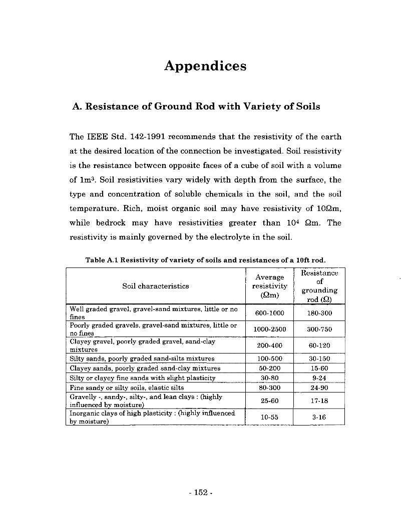
Appendices

A. Resistance of Ground Rod with Variety of Soils

The IEEE Std. 142-1991 recommends that the resistivity of the earth

at the desired location of the connection be investigated. Soil resistivity

is the resistance between opposite faces of a cube of soil with a volume

of lm3. Soil resistivities vary widely with depth from the surface, the

type and concentration of soluble chemicals in the soil, and the soil

temperature. Rich, moist organic soil may have resistivity of lOQm,

while bedrock may have resistivities greater than 104 flm. The

resistivity is mainly governed by the electrolyte in the soil.

Table A.l Resistivity of variety of soils and resistances of a 10ft rod.

Soil characteristics Average

resistivity (Qm)

Resistance of

grounding rod (£2)

Well graded gravel, gravel-sand mixtures, little or no fines

600-1000 180-300

Poorly graded gravels, gravel-sand mixtures, little or no fines

1000-2500 300-750

Clayey gravel, poorly graded gravel, sand-clay mixtures

200-400 60-120

Silty sands, poorly graded sand-silts mixtures 100-500 30-150 Clayey sands, poorly graded sand-clay mixtures 50-200 15-60 Silty or clayey fine sands with slight plasticity 30-80 9-24 Fine sandy or silty soils, elastic silts 80-300 24-90 Gravelly -, sandy-, silty-, and lean clays : (highly influenced by moisture)

25-60 17-18

Inorganic clays of high plasticity : (highly influenced by moisture)

10-55 3-16

- 152 -

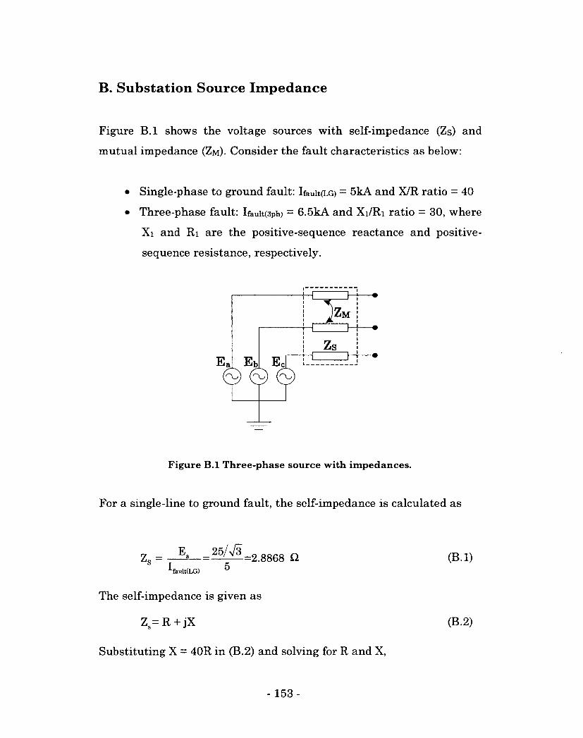
B. Substation Source Impedance

Figure B.l shows the voltage sources with self-impedance (Zs) and

mutual impedance (ZM)- Consider the fault characteristics as below:

• Single-phase to ground fault: IFAUIT(LG) = 5kA and X/R ratio = 40

• Three-phase fault: Ifauit(3ph) = 6.5kA and X1/R1 ratio = 30, where

Xi and Ri are the positive-sequence reactance and positive-

sequence resistance, respectively.

For a single-line to ground fault, the self-impedance is calculated as

Zs

Figure B.l Three-phase source with impedances.

fault(LG)

(B.l)

The self-impedance is given as

Zs= R + jX (B.2)

Substituting X = 40R in (B.2) and solving for R and X,

- 153 -

Zs = 0.072 + j2.8858 Q .

Similarly, for a three-phase symmetrical fault, the positive-sequence

impedance is given as

Zj = —^— = 25^= 2.2206 Q. (B.3) ^•fault(3ph) 6-5

Substituting Xi = 30Ri into Zi = Ri+jXi and solving for Ri and Xi,

Zi = 0.0740+ j2.2193 Q.

Also

^1 ~ Zs"

ZM = Zs - Zi = - 0.0018 + j0.6665 Q.

- 154 -

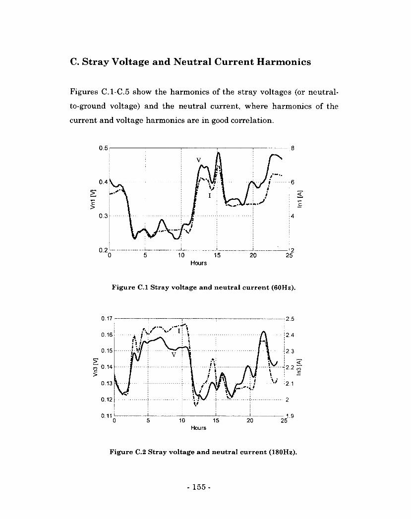
C. Stray Voltage and Neutral Current Harmonics

Figures C.1-C.5 show the harmonics of the stray voltages (or neutral-

to-ground voltage) and the neutral current, where harmonics of the

current and voltage harmonics are in good correlation.

Hours

Figure C.l Stray voltage and neutral current (60Hz).

0.17 2.5

0.16 2.4

0.15 2.3

0.14 2.2

0.13

0.12

11 0 20 25

Hours

Figure C.2 Stray voltage and neutral current (180Hz).

- 155-

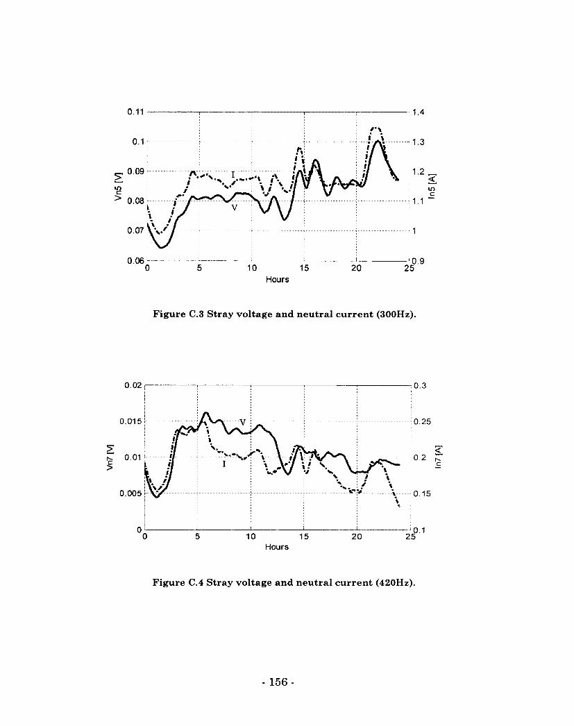
lO c >

0.11

0.1

0.09

0.08

0.07

0.06'

f'\ « '\

+'S. I

!\ i\

% . ' A i\ !f\

\J/\

A

l / w if i if \

}J \

w V

A V f

10 15 Hours

20

1.4

1.3

1.2

1.1

in c

- ' 0 . 9 25


0.02

0.015

£

0.005

if if il

1 // » il V '/ \* • # Y\y

A/A V \ vv. 1 V

I \ 'ft \ A7 < u* V / \ ^ \ v *» Vn V p A"

\

i

0.3

10 15 Hours

20

0 25

< 0 . 2 "

0.15

25 0.1


- 156 -

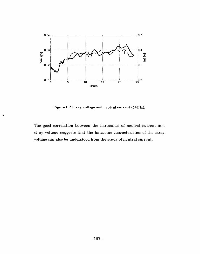
Hours


The good correlation between the harmonics of neutral current and

stray voltage suggests that the harmonic characteristics of the stray

voltage can also be understood from the study of neutral current.

- 157 -

University of Alberta - Bibliothèque et Archives Canada

Documents