NUMERICAL LINEAR ELASTIC INVESTIGATION OF STEEL ROOF DECK DIAPHRAGM BEHAVIOUR ACCOUNTING FOR THE CONTRIBUTION OF NON- STRUCTURAL COMPONENTS By Simon Mastrogiuseppe McGill Department of Civil Engineering and Applied Mechanics McGill University, Montréal, Québec, Canada February, 2006 A thesis submitted to the Faculty of Graduate and Postdoctoral Studies in partial fulfillment of the requirements of the degree of Master of Engineering © Simon Mastrogiuseppe, 2006

Welcome message from author
This document is posted to help you gain knowledge. Please leave a comment to let me know what you think about it! Share it to your friends and learn new things together.
Transcript

NUMERICAL LINEAR ELASTIC INVESTIGATION OF
STEEL ROOF DECK DIAPHRAGM BEHA VIOUR
ACCOUNTING FOR THE CONTRIBUTION OF NON
STRUCTURAL COMPONENTS
By
Simon Mastrogiuseppe
~ McGill
Department of Civil Engineering and Applied Mechanics
McGill University, Montréal, Québec, Canada
February, 2006
A thesis submitted to the Faculty of Graduate and
Postdoctoral Studies in partial fulfillment of the requirements
of the degree of Master of Engineering
© Simon Mastrogiuseppe, 2006

1+1 Library and Archives Canada
Bibliothèque et Archives Canada
Published Heritage Branch
Direction du Patrimoine de l'édition
395 Wellington Street Ottawa ON K1A ON4 Canada
395, rue Wellington Ottawa ON K1A ON4 Canada
NOTICE: The author has granted a nonexclusive license allowing Library and Archives Canada to reproduce, publish, archive, preserve, conserve, communicate to the public by telecommunication or on the Internet, loan, distribute and sell theses worldwide, for commercial or noncommercial purposes, in microform, paper, electronic and/or any other formats.
The author retains copyright ownership and moral rights in this thesis. Neither the thesis nor substantial extracts from it may be printed or otherwise reproduced without the author's permission.
ln compliance with the Canadian Privacy Act some supporting forms may have been removed from this thesis.
While these forms may be included in the document page cou nt, their removal does not represent any loss of content from the thesis.
• •• Canada
AVIS:
Your file Votre référence ISBN: 978-0-494-24996-3 Our file Notre référence ISBN: 978-0-494-24996-3
L'auteur a accordé une licence non exclusive permettant à la Bibliothèque et Archives Canada de reproduire, publier, archiver, sauvegarder, conserver, transmettre au public par télécommunication ou par l'Internet, prêter, distribuer et vendre des thèses partout dans le monde, à des fins commerciales ou autres, sur support microforme, papier, électronique et/ou autres formats.
L'auteur conserve la propriété du droit d'auteur et des droits moraux qui protège cette thèse. Ni la thèse ni des extraits substantiels de celle-ci ne doivent être imprimés ou autrement reproduits sans son autorisation.
Conformément à la loi canadienne sur la protection de la vie privée, quelques formulaires secondaires ont été enlevés de cette thèse.
Bien que ces formulaires aient inclus dans la pagination, il n'y aura aucun contenu manquant.

ABSTRACT
Dynamic analysis programs and empirical fonnulae are often used to compute the period of
vibration of single-storey steel buildings. Recent ambient vibration tests of buildings in
Québec and British Columbia have shown that the predicted period of vibration is typically
much longer than that measured. Software and empirical fonnulae do not usually take into
account the stiffening effects of the non-structural components; this could be the source of the
discrepancy between the results in the field and the results obtained by computational
methods.
This research project concentrates on the roof diaphragm system of single-storey steel
buildings and the contribution of the non-structural components to diaphragm stifihess. It is
believed that the non-structural components, roofing materials such as gypsum board and
fibreboard, add to the overall stifihess ofthe system. A roofing system called AMCQ SBS-34
consisting of gypsum board, ISO insulation board and fibreboard, aU hot bitumen adhered,
was studied. The full roof system, as weIl as its individual components and connections, were
first studied through laboratory testing. The flexural and shear stifihess of the fibreboard and
gypsum panels, as well as the shear stifihess and equivalent flexural stifihess of the complete
roof system and shear stiffuess of the roofing connections were detennined.
Linear elastic finite element models, using the SAP2000 software, were developed to
replicate the behaviour ofbare sheet steel and clad diaphragm test specimens. The test based
properties of the roofing components and connections were incorporated into the definition of
the elements. The models were then calibrated based on the results of large-scale diaphragm
tests by Yang. Once the elastic behaviour of the diaphragms had been matched, a parametric
study was perfonned in order to assess the importance of the contribution of the roofing
assembly relative to the roof deck panel thickness.
It was shown that as the deck thickness increases, the relative contribution of the non
structural components decreases on a percentage basis, but does not become non-negligible.
The increase in shear stifihess of the diaphragm ranges from 58.6% for the 0.76 mm deck
panel to 4.7% for the 1.51 mm roof deck panel, dependent on the sidelap and deck-to-frame
connection configuration.

RÉSUMÉ
Les programmes d'analyse dynamique et les formules empiriques sont souvent utilisés
pour calculer la fréquence naturelle de vibration de bâtiments à un étage en acier. De
récents résultats expérimentaux au Québec et en Colombie-Britannique démontrent que
ces analyses donnent des périodes beaucoup plus longues qu'avec des tests in-situ. Les
programmes d'analyse dynamique et les formules empiriques ne prennent pas en
considération les effets de renforcement des éléments non-structuraux: ces éléments
pourraient être la source de la différence entre les résultats in-situ et les analyses
numériques.
Ce projet porte sur le diaphragme de toit et la contribution des éléments non-structuraux à
la rigidité du diaphragme. On croit que les éléments non-structuraux - tels que les
matériaux de toiture du type panneaux de gypse ou fibre de bois - ajoutent à la rigidité du
système. Une combinaison de toiture appelée AMCQ SBS-34, composée de panneaux de
gypse, d'isolant en polyisocyanurate et de fibre de bois, a été étudiée. Les rigidités en
flexion et en cisaillement des composantes ont été déterminées séparément; de plus, la
rigidité en cisaillement et la rigidité équivalente en flexion de la combinaison de toiture
ont été déterminées.
Des modèles éléments finis, bâtis avec le logiciel SAP2000, ont été développés afin de
reproduire le comportement du diaphragme de toit sans et avec les composantes non
structurales. Les modèles, une fois bâti, ont été calibrés à partir des données
expérimentales obtenues par Yang. Une fois le modèle calibré, une étude paramétrique
est effectuée afin de déterminer la contribution relative des éléments non-structuraux à la
rigidité totale du diaphragme selon l'épaisseur du tablier métallique.
Il a été démontré que la contribution relative des composantes non-structurales diminue
lorsque l'épaisseur du tablier d'acier augmente, mais elle ne devient pas non-négligeable.
L'augmentation de la rigidité varie de 58.6% pour le tablier de 0.76 mm d'épaisseur à
4.7% pour le tablier de 1.51 mm, dépendamment de la configuration des connecteurs à la
structure et des connecteurs de couture.
11

ACKNOWLEDGEMENTS
First off, 1 would like to thank Professor Colin A. Rogers. Without your support,
kindness, guidance and constant input, this thesis would never have been completed.
Your constant presence during the whole two years of this project made is not only
possible, but thoroughly enjoyable. Thank you.
1 would also like to mention Prof essor Robert Tremblay from École Polytechnique de
Montréal. Your help in determining the direction of this study as weIl as for yOUf input
along the way were much appreciated.
1 would also like to thank the following people:
• Steve Kecani and Eddie Del Campo from the Department of Physics machine
shop. Thanks for helping me keep my fingers.
• Ronald Sheppard, Damon Kiperchuk, Marek Przykorski and John Bartczak.
Without yOUf help, 1 would not have finished.
• Denis Fortier for helping me decipher the ASTM drawings.
• Dr. William Cook, for saving my hard drive.
• Everybody in the civil administrative staff.
Special thanks to Camelia Dana Nedisan for yOUf help. It was a pleasure working with
you.
The following organizations and companies are highly appreciated for their contributions
on this project: the Natural Sciences and Engineering Research Council of Canada
(NSERC); The Canam Group Ltd.; Hilti Limited; André at Toitures Couture Inc.; André
at Anica Steel Inc.
Last but not least, 1 would like to thank my family and Caroline for their support and their
belief in me.
III
TABLE OF CONTENTS
Abstract. _________________________ _
Résumé __________________________ ll
Acknowledgements iii
Table of Contents iv
List of Figures ________________________ Vlll
List of Tables XVll
List of Symbols XIX
1
2
INTRODUCTION 1
1.1 General _______________________ 1
1.2
1.3
Statement ofproblem
Objectives
___________________3 _______________________ 4
1.4
1.5
Scope and Limitation of Study
Thesis outline
________________5 _____________________6
LITERA TURE REVIEW 7
2.1 General 7
2.2 Nilson 7
2.3 Luttrell 7
2.4 Tremblay and Stiemer 8
2.5 Medhekar 8
2.6 Rogers and Tremblay 10
2.7 Essa et al. 11
2.8 Martin 12
2.9 Nedisan 14
2.10 Yang 14
2.11 Lamarche 19
2.12 Turek 20
2.13 2005 NBCC 21
2.14 CSA S16 22
IV
2.15 Summary 23
3 MATERIAL AND CONNECTION EXPERIMENTS 24
3.1 General 24
3.2 Two-Sided Shear Test 24
3.2.1 Setup and Test Procedure 24
3.2.2 Test Specimens 26
3.2.3 Specimen Behaviour 27
3.2.3.1 Fibreboard 27
3.2.3.2 Gypsum Board 28
3.2.4 Data Analysis 29
3.2.5 Discussion 31
3.3 Flexural Test 34
3.3.1 Setup and Test Procedure 34
3.3.2 Test Specimens 34
3.3.3 Specimen Behaviour 36
3.3.3.1 Fibreboard 36
3.3.3.2 Gypsum Board 38
3.3.4 Data Analysis 41
3.3.4.1 Fibreboard Specimens 42
3.3.4.2 Gypsum board Specimens 43
3.3.5 Discussion 44
3.4 Four-Sided Shear Test 47
3.4.1 Setup and Test Procedure 47
3.4.2 Test Specimens 50
3.4.3 Specimen Behaviour 54
3.4.3.1 Unstiffened Specimens 54
3.4.3.1.1 Addition of Stiffeners 55
3.4.3.2 FB-STIFF (Stiffened Fibreboard) 56
3.4.3.3 GYP-STIFF (Stiffened Gypsum Board) 57
3.4.3.4 FB+ISO 58
v
3.4.3.5 FULL SECTION 60
3.4.4 Data Analysis 62
3.4.5 Discussion 65
3.4.5.1 Concentric Load Analysis 65
3.4.5.2 Finite Element Analysis 68
3.5 Connection Tests 70
3.5.1 Setup and Test Procedure 70
3.5.2 Test Specimens 72
3.5.2.1 Deck-to-Frame 72
3.5.2.2 Sidelap 72
3.5.2.3 Gypsum-to-Deck 73
3.5.3 Specimen Behaviour 74
3.5.3.1 Deck -to-frame 74
3.5.3.2 Sidelap 75
3.5.3.3 Gypsum-to-Deck 76
3.5.4 Data Analysis 77
3.5.5 Discussion 80
3.6 Conclusion 81
4 ELASTIC DIAPHRAGM ANALYSES 82
4.1 General 82
4.2 Roof Diaphragm Tests by Yang 82
4.2.1 Frame Setup 82
4.2.2 Specimen Configurations 84
4.2.3 Diaphragm Test Results 89
4.2.3.1 Test 43 90
4.2.3.2 Test 45 92
4.3 SAP2000 Models by Yang 94
4.3.1 General Information 94
4.3.2 Yang Elements 96
4.4 SAP2000 Models of Full Size Test Diaphragms 98
VI

4.4.1 General Information 98
4.4.2 Elements 102
4.4.2.1 Material Properties 102
4.4.2.2 Shell Elements 103
4.4.2.3 Link Elements 105
4.4.2.4 Frame Elements 107
4.4.3 Analysis Parameters 108
4.4.4 Model Specifie Properties 110
4.4.4.1 Multi-Linear Link Elements 110
4.4.4.2 Joint Constraints 110
4.5 Data Analysis, Results and Discussion 112
4.6 SDI Results and Discussion 117
4.7 Influence of Non-Structural Components on Diaphragm Stiffness:
Parametric Study 120
4.7.1 General Information 121
4.7.2 SDI Connector Stiffness 122
4.7.3 Results 122
5 CONCLUSION AND RECOMMENDATIONS 124
5.1 Conclusions ___________________ 124
5.2 Recommendations 127
REFERENCES ____________________ 129
APPENDIX A: TWO-SIDED SHEAR TEST DATA _________ 136
APPENDIX B: FLEXURAL TEST DATA 140
APPENDIX C: FOUR-SIDED SHEAR TEST DATA 156
APPENDIX D: CONNECTION TEST DATA 179
APPENDIX E: SAP2000 INPUT/OUTPUT FILE EXCERPTS 189
APPENDIX F: SDI CALCULATION EXCEL WORKSHEETS 195
vu
LIST OF FIGURES
Figure 1.1 Typical structural arrangement of a single storey steel building
(Rogers & Tremblay (2000)) 1
Figure 1.2 Non-structural roofing components 2
Figure 1.3 Roofing cross-section as tested by Yang (2003) 2
Figure 1.4 Periods of vibration 4
Figure 2.1 Roofing cross-section as tested by Yang (2003) 15
Figure 2.2 Undeformed shapes ofbare sheet steel deck and deck with
gypsum elements 18
Figure 3.1 Two-sided shear setup (Boudreault, 2005) 25
Figure 3.2 Gypsum shear test specimen 27
Figure 3.3 Fibreboard specimens - shear load vs. shear deformation 28
Figure 3.4 Gypsum board specimens - shear load vs. shear deformation 29
Figure 3.5 Deformation of steel deck and non-structural components
under shear load - Test 45 (Yang, 2003) 32
Figure 3.6 Comparison of gypsum board and fibreboard specimens -
shear load vs. shear deformation 33
Figure 3.7 Flexural test setup 34
Figure 3.8 Flexural test results - FI to F 16 36
Figure 3.9 Flexural test results - FDA and FDB 37
Figure 3.10 Flexuraltest results - G-pp 1 to G-pp Il 38
Figure 3.11 Flexural test results - G-PP12 to G-PP22 39
Figure 3.12 Flexural test results - G-PL1 to G-PL11 40
Figure 3.13 Flexural test results ~ G-PLI2 to GPL22 41
Figure 3.14 Flexural test results - G-PP vs. G-PL 46
Figure 3.15 Flexural test results - FB vs. G-PP vs. G-PL 47
Figure 3.16 Four-sided shear test frame 48
Figure 3.17 Hinge area close-up 49
Figure 3.18 Test specimen dimensions 50
Figure 3.19 Fibreboard and gypsum board specimens 51
Figure 3.20 Fibreboard specimen; hot bitumen application 51
Vlll
Figure 3.21 FB+ISO specimen plan view; FB+ISO specimen cross-section view _52
Figure 3.22 FULL SECTION specimen plan view; FULL SECTION specimen
cross-section view 53
Figure 3.23 FULL SECTION specimen in test frame before 54
Figure 3.24 Panelload forces 55
Figure 3.25 Stiffener installed on gypsum board panel 56
Figure 3.26 Stiffened fibreboard -load vs. elongation 57
Figure 3.27 Stiffened gypsum board -load vs. elongation 58
Figure 3.28 FB+ISO -load vs. elongation 59
Figure 3.29 FULL SECTION -load vs. elongation 60
Figure 3.30 Specimen free body diagram 61
Figure 3.31 Roof cross-section (Yang, 2003) 66
Figure 3.32 Spring-stiffuess diagram of non-structural roofing components 67
Figure 3.33 Modified spring-stiffness diagram of non-structural roofing
components 67
Figure 3.34 Undeformed and deformed FEM of FULL SECTION test specimen __ 69
Figure 3.35 Undeformed and deformed Shear Model 70
Figure 3.36 4 L VDT connection test setup gypsum test; 8 LVDT
connection test setup sidelap and deck-to-frame ________ 71
Figure 3.37 Typical deck-to-frame connection test specimen 73
Figure 3.38 Typical sidelap connection test specimen 73
Figure 3.39 Typical gypsum-to-deck connection test specimen 74
Figure 3.40 Screw and washer assembly used for gypsum-to-deck connections __ 74
Figure 3.41 Deck-to-frame connection -load vs. displacement 75
Figure 3.42 Sidelap connection -load vs. displacement 76
Figure 3.43 Gypsum-to-deck connection -load vs. displacement _______ 77
Figure 4.1
Figure 4.2
Figure 4.3
Figure 4.4
Plan view of frame setup (Essa et al., 2001) __________ 83
Diaphragm test setup (schematic plan view) 83
Hilti X-ENDK22-THQI2 nail and connection detail;
Hilti S-MD 12-14xl HWH #1 F.P. screw (Yang, 2003) _____ 84
Plan of Group 3 test layout (Yang, 2003) 85
IX

Figure 4.5 Roofing cross-section (Yang, 2003) 86
Figure 4.6 Gypsum-to-deck assemblies (Yang, 2003) 87
Figure 4.7 Steel deck installed on test frame (Yang, 2003) 87
Figure 4.8 Gypsum board layout (Yang, 2003) 88
Figure 4.9 Roofassembly procedure (Yang, 2003) 89
Figure 4.10 Warping deformation of steel deck profile (Yang, 2003) 90
Figure 4.11 Normalized shear vs. rotation curve of Test 43 (Yang, 2003) 91
Figure 4.12 Sheet buckling, screw tilt and pull out at C20 (Yang, 2003) 91
Figure 4.13 Deck-to-frame slip and bearing, tearing damage of
sheet steel at III (Yang, 2003) 92
Figure 4.14 Steel sheet deformation during loading, flute width enlarged; steel sheet
deformation during loading, flute width reduced (Yang, 2003) 93
Figure 4.15 Steel deck flute height diminished, gypsum board cracked
(Yang, 2003) _________________ 93
Figure 4.16 Warping deformation of steel deck and cracking ofgypsum
board (Yang, 2003) ________________ 93
Figure 4.17 Normalized shear vs. rotation curve of Test 45 (Yang, 2003) 94
Figure 4.18 Cantilever analysis model; Frame &joists; sheet layout (Yang, 2003) _95
Figure 4.19 Undeformed and deformed shape of small-scale steel deck
model (Yang, 2003) ________________ 95
Figure 4.20 Undeformed and deformed shape of small-scale steel
deck model with roofing elements (Yang, 2003) 96
Figure 4.21 Gap property types shown for axial deformations (CSL 2002) 97
Figure 4.22 Cantilever analysis model 99
Figure 4.23 Undeformed shape offull-scale steel deck model 101
Figure 4.24 Undeformed shape of full-scale steel deck model with
roofing elements 101
Figure 4.25 Multi-linear spring stiffness of GAP element 107
Figure 4.26 Support; Frame element and end releases 108
Figure 4.27 M-L (GAP) link element typicallocation 110
Figure 4.28 NL 1 link element with joint constraint 111
x

Figure 4.29 Deformed shape ofbare steel deck 113
Figure 4.30 Close-up ofwarping ofbare steel deck 114
Figure 4.31 Deformed shape of steel deck with roofing components 114
Figure 4.32 Close-up of warping for steel deck with roofing components 115
Figure 4.33 Deformation of non-structural components 115
Figure Al FB Test 2 138
Figure A2 FB Test 3 138
Figure A3 FB Test 4 138
Figure A4 FB Test 5 138
Figure A5 FB Test 6 138
Figure A6 GYP Test 1 139
Figure A7 GYP Test 2 139
Figure A8 GYP Test 3 139
Figure A9 GYP Test 4 139
Figure BI FBl 147
Figure B2 FB2 147
Figure B3 FB3 147
Figure B4 FB4 147
Figure B5 FB5 147
Figure B6 FB6 147
Figure B7 FB7 147
Figure B8 FB8 147
Figure B9 FB9 148
Figure BIO FBIO 148
Figure Bll FBll 148
Figure B12 FB12 148
Figure B13 FB13 148
Figure B14 FB14 149
Figure B15 FB15 148
Figure B16 FB16 148
Figure B17 FDA-l 149
Xl
Figure B18 FDA-2 149
Figure B19 FDA-3 149
Figure B20 FDA-4 149
Figure B21 FDB-l 149
Figure B22 FDB-2 149
Figure B23 FDB-3 149
Figure B24 FBD-4 149
Figure B25 G-PLI 150
Figure B26 G-PL2 150
Figure B27 G-PL3 150
Figure B28 G-PL4 150
Figure B29 G-PL5 150
Figure B30 G-PL6 150
Figure B31 G-PL7 150
Figure B32 G-PL8 150
Figure B33 G-PL9 151
Figure B34 G-PLI0 151
Figure B35 G-PLll 151
Figure B36 G-PLI2 151
Figure B37 G-PL13 151
Figure B38 G-PLI4 151
Figure B39 G-PLI5 151
Figure B40 G-PLI6 151
Figure B41 G-PLI7 152
Figure B42 G-PLI8 152
Figure B43 G-PLI9 152
Figure B44 G-PL20 152
Figure B45 G-PL21 152
Figure B46 G-PL22 152
Figure B47 G-PPI 152
Figure B48 G-PP2 152
Xll
Figure B49 G-PP3 153
Figure B50 G-PP4 153
Figure B51 G-PP5 153
Figure B52 G-PP6 153
Figure B53 G-PP7 153
Figure B54 G-PP8 153
Figure B55 G-PP9 153
Figure B56 G-PPIO 153
Figure B57 G-PPII 154
Figure B58 G-PPI2 154
Figure B59 G-PP13 154
Figure B60 G-PP14 154
Figure B61 G-PPI5 154
Figure B62 G-PP16 154
Figure B63 G-PP17 154
Figure B64 G-PP18 154
Figure B65 G-PP19 155
Figure B66 G-PP20 155
Figure B67 G-PP21 155
Figure B68 G-PP22 155
Figure Cl FB 1 load vs. elongation 157
Figure C2 FB2 load vs. elongation 158
Figure C3 FB3 load vs. elongation 159
Figure C4 FB4+FB5 load vs. elongation 160
Figure C5 GYP 1 load vs. elongation 161
Figure C6 FB-2 STIFF load vs. elongation 162
Figure C7 FB-3 STIFF load vs. elongation 163
Figure C8 FB-4 STIFF load vs. elongation 164
Figure C9 FB-5 STIFF load vs. elongation 165
Figure CIO GYP-1 STIFF load vs. elongation 166
Figure CU GYP-2 STIFF load vs. elongation 167
X111
Figure C12 GYP-3 STIFF load vs. elongation 168
Figure C13 GYP-4 STIFF load vs. elongation 169
Figure C14 GYP-5 STIFF load vs. elongation 170
Figure C15 GYP-6 STIFF load vs. elongation 171
Figure C16 FB+ISO 1 load vs. elongation 172
Figure C17 FB+ISO 2 load vs. elongation 173
Figure C18 FB+ISO 3 load vs. elongation 174
Figure C19 FULL SECTION load vs. elongation 175
Figure C20 FULL SECTION load vs. elongation 176
Figure C21 FULL SECTION load vs. elongation 177
Figure C22 FULL SECTION load vs. elongation 178
Figure Dl 076-N-A 180
Figure D2 076-N-B 180
Figure D3 076-N-C 180
Figure D4 076-N-D 180
Figure D5 076-N-E 180
Figure D6 076-N-H 180
Figure D7 076-N-I 180
Figure D8 091-N-A 180
Figure D9 091-N-B 181
Figure DIO 091-N-C 181
Figure D11 091-N-D 181
Figure D12 091-N-E 181
Figure D13 091-N-H 181
Figure D14 091-N-I 181
Figure D15 122-N-A 181
Figure D16 122-N-B 181
Figure D17 122-N-C 182
Figure D18 122-N-D 182
Figure D19 122-N-E 182
Figure D20 122-N-H 182
XIV

Figure D21 122-N-I 182
Figure D22 151-N-A 182
Figure D23 151-N-B 182
Figure D24 151-N-C 182
Figure D25 151-N-D 183
Figure D26 151-N-E 183
Figure D27 151-N-H 183
Figure D28 151-N-I 183
Figure D29 076-S-A 183
Figure D30 076-S-B 183
Figure D31 076-S-C 183
Figure D32 076-S-D 183
Figure D33 076-S-E 184
Figure D34 076-S-H 184
Figure D35 076-S-1 184
Figure D36 091-S-A 184
Figure D37 091-S-B 184
Figure D38 091-S-C 184
Figure D39 091-S-D 184
Figure D40 091-S-E 184
Figure D41 091-S-H 185
Figure D42 091-S-1 185
Figure D43 122-S-A 185
Figure D44 122-S-B 185
Figure D45 122-S-C 185
Figure D46 122-S-D 185
Figure D47 122-S-E 185
Figure D48 122-S-H 185
Figure D49 122-S-1 186
Figure D50 151-S-A 186
Figure D51 151-S-B 186
xv

Figure D52 151-S-C 186
Figure D53 151-S-D 186
Figure D54 151-S-E 186
Figure D55 151-S-H 186
Figure D56 076-G-A 186
Figure D57 076-G-B 187
Figure D58 076-G-C 187
Figure D59 076-G-D 187
Figure D60 076-G-E 187
Figure D61 091-G-A 187
Figure D62 091-G-B 187
Figure D63 091-G-C 187
Figure D64 091-G-D 187
Figure D65 122-G-A 188
Figure D66 122-G-B 188
Figure D67 122-G-C 188
Figure D68 122-G-D 188
Figure D69 151-G-A 188
Figure D70 151-G-B 188
Figure D71 151-G-C 188
Figure D72 151-G-D 188
Figure FI SDI 38-76-6-NS-M calculation sheet 196
Figure F2 SDI 38-91-6-NS-M calculation sheet 197
Figure F3 SDI 38-122-6-NS-M calculation sheet 198
Figure F4 SDI 38-151-6-NS-M calculation sheet 199
Figure F5 SDI* 38-76-6-NS-M calculation sheet 200
Figure F6 SDI* 38-91-6-NS-M calculation sheet 201
Figure F7 SDI** 38-76-6-NS-M calculation sheet 202
Figure F8 SDI** 38-91-6-NS-M calculation sheet 203
Figure F9 SDI** 38-122-6-NS-M calculation sheet 204
Figure F10 SDI** 38-151-6-NS-M calculation sheet 205
XVI

LIST OF TABLES
Table 2.1 Connection stiffness values (Rogers and Tremblay, 2003) 10
Table 2.2 Test series results conducted by Essa et al. (2001, 2003) 12
Table 2.3 Large-scale diaphragm test series by Martin (2002) 13
Table 2.4 Large-scale diaphragm test series by Yang (2003) 17
Table 2.5 Shear stiffness (Yang, 2003) 19
Table 3.1 Two-sided shear test - fibreboard results 31
Table 3.2 Two-sided shear test - gypsum results 31
Table 3.3 Flexural test - fibreboard results 43
Table 3.4 Flexural test - gypsum results 44
Table 3.5 Four-sided shear test results 64
Table 3.6 Deck-to-frame connection stiffness 78
Table 3.7 Sidelap connection stiffness 79
Table 3.8 Gypsum-to-deck connection stiffness 79
Table 3.9 Gypsum-to-deck connection average stiffness 80
Table 4.1 Large-scale diaphragm test results (Yang, 2003) 90
Table 4.2 Properties used by Yang in SAP models 98
Table 4.3 SAP2000 - material properties 103
Table 4.4 SAP2000 - shell element thickness (mm) 104
Table 4.5 SAP2000 - link properties (kN/mm) 105
Table 4.6 SAP2000 - frame element properties 108
Table 4.7 SAP2000 non-linear analysis parameters 109
Table 4.8 Analytical model displacements and stiffnesses 113
Table 4.9 Connection stiffness used for SDr calculation (kN/mm) 119
Table 4.10 SAP vs. SDr prediction ofbare steel diaphragm stiffness (kN/mm) _119
Table 4.11 SAP -link properties (kN/mm) 122
Table 4.12 SAP - diaphragm stiffness G' (kN/mm) 122
Table 4.13 rncrease in G' stiffness with gypsum board 122
Table Al Fibreboard and gypsum board specimen thickness 137
Table A2 Fibreboard and gypsum board specimen width 137
Table A3 Fibreboard and gypsum board maximum load 137
XVll
Table BI Fibreboard specimen thickness (mm) 141
Table B2 Fibreboard specimen width (mm) 142
Table B3 Gypsum board specimen thickness (mm) 143
Table B4 Gypsum board specimen width (mm) 144
Table B5 Fibreboard specimen ultimate load (N) 145
Table B6 Gypsum board specimen ultimate load (N) 146
Table Cl FBl data 157
Table C2 FB2 data 158
Table C3 FB3 data 159
Table C4 FB4+FB5 data 160
Table C5 GYP-l data 161
Table C6 FB-2 STIFF data 162
Table C7 FB-3 STIFF data 163
Table C8 FB-4 STIFF data 164
Table C9 FB-5 STIFF data 165
Table CIO GYP-l STIFF data 166
Table CIl GYP-2 STIFF data 167
Table C12 GYP-3 STIFF data 168
Table C13 GYP-4 STIFF data 169
Table C14 GYP-5 STIFF data 170
Table C15 GYP-6 STIFF data 171
Table C16 FB+ISO 1 data 172
Table C17 FB+ISO 2 data 173
Table C18 FB+ISO 3 data 174
Table C19 FULL SECTION 1 data 175
Table C20 FULL SECTION 2 data 176
Table C21 FULL SECTION 3 data 177
Table C22 FULL SECTION 4 data 178
XVlll
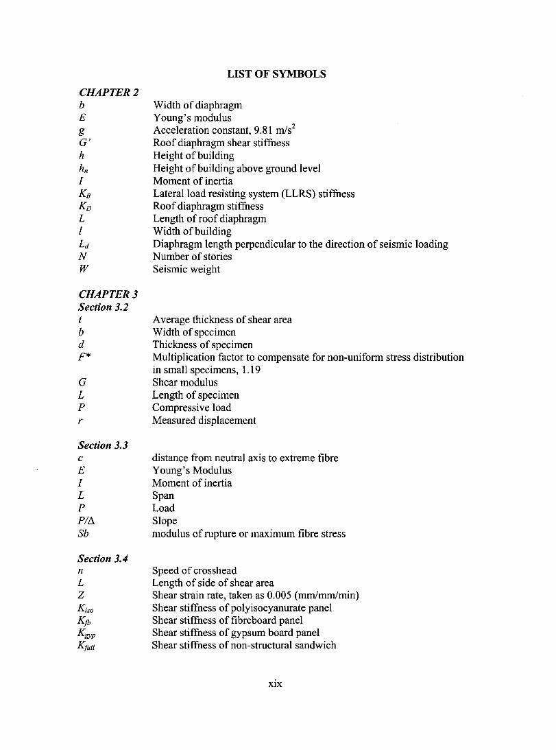
CHAPTER2 b E g G' h hn
1 KB
KD L 1 Ld N W
CHAPTER3 Section 3.2 t b d F*
G L P r
Section 3.3 c E 1 L P PI/). Sb
Section 3.4 n L Z Kiso
Kjb Kgyp
Kfull
LIST OF SYMBOLS
Width of diaphragm Young's modulus Acceleration constant, 9.81 m/s2
Roof diaphragm shear stiffness Height of building Height of building above ground level Moment of inertia Lateralload resisting system (LLRS) stiffness Roof diaphragm stiffness Length of roof diaphragm Width of building Diaphragm length perpendicular to the direction of seismic loading Number of stories Seismic weight
Average thickness of shear area Width of specimen Thickness of specimen Multiplication factor to compensate for non-uniform stress distribution in small specimens, 1.19 Shear modulus Length of specimen Compressive load Measured displacement
distance from neutral axis to extreme fibre Young's Modulus Moment of inertia Span Load Slope modulus of rupture or maximum fibre stress
Speed of crosshead Length of side of shear area Shear strain rate, taken as 0.005 (mm/mm/min) Shear stiffness of polyisocyanurate panel Shear stiffness of fibre board panel Shear stiffness of gypsum board panel Shear stiffness of non-structural sandwich
XIX

CHAPTER4 L A P S !!l
'Y G' !!ls !!lD !!le E t
C s d (jJ
Modellength, 6096 mm Model width, 3657.6 mm Unit point load Unit shear force, PIL y -direction deflection due to P Shear distortion, !!lIA Diaphragm shear stiffness Shear displacement Diaphragm warping displacement Connection displacement Young's modulus Base metal thickness Connector slip parameter Girth of corrugation per rib Corrugation pitch Reduction factor based on number of equal spans
xx
1.1 General
CHAPTERI
INTRODUCTION
Single-storey steel buildings make up a large percentage of the building stock in the light
industrial and commercial industry. These buildings can be located in regions of
moderate or active seismicity levels, such as the west coast of British Columbia and the
St. Lawrence and Ottawa River valleys. The lateral force resisting system is often
composed of concentrically braced frames (CBFs) placed on the perimeter of the building
and a flexible steel roof deck diaphragm. When these structures undergo wind or
earthquake loading, the forces flow from the roof diaphragm into the braced frames and
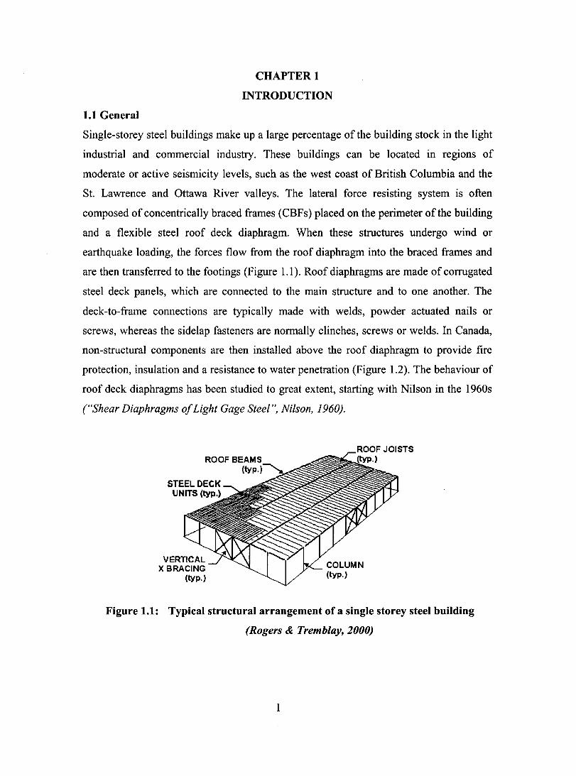
are then transferred to the footings (Figure 1.1). Roof diaphragms are made of corrugated
steel deck panels, which are connected to the main structure and to one another. The
deck-to-frame connections are typically made with welds, powder actuated nails or
screws, whereas the sidelap fasteners are normally clinches, screws or welds. In Canada,
non-structural components are then installed above the roof diaphragm to provide tire
protection, insulation and a resistance to water penetration (Figure 1.2). The behaviour of
roof deck diaphragms has been studied to great extent, starting with Nilson in the 1960s
("Shear Diaphragms of Light Gage Steel ", Ni/son, 1960).
Figure 1.1: Typical structural arrangement of a single storey steel building
(Rogers & Tremblay, 2000)
1

Figure 1.2: Non-structural roofing components
Figure 1.3: Roofing cross-section as tested by Yang (2003)
A research program on the behaviour of roof deck diaphragms under seismic loading has
been underway since 1999 at École Polytechnique of Montreal and McGill University.
Numerous bare steel diaphragm specimens featuring different connection configurations
and deck thickness have been tested to evaluate their inelastic performance (Es sa et al.
(2001), Martin (2002), Yang (2003». Yang also carried out tests oftwo diaphragms that
2
were constructed with non-structural components (Figure 1.3). It has been shown that
there is a significant difference in stiffness, strength and ductility depending mainly on
the connection detailing. However, the contribution of the non-structural components to
the roof diaphragm stiffness and strength is also of importance. These components cause
an increase in both the stiffness and strength according to Yang. Additional studies to
identify the period of vibration of low-rise buildings have been completed at the
University of Sherbrooke (Lamarche, 2005) and at the University of British Columbia
(Turek and Ventura, 2005). These ambient vibration tests have revealed that there exists a
discrepancy between the building period used for seismic design, as obtained from the
2005 National Building Code of Canada (NBCC) (NRCC, 2005) and from dynamic
analyses, compared with that which the buildings actually possess. It is possible that the
non-structural roofing components are, in part, responsible for a shortening of the natural
period of vibration.
1.2 Statement of Problem
The opportunity for engineers to carry out dynamic analyses has increased with the
advent of powerful analysis tools. In many design situations, it has become necessary to
use software to estimate the dynamic characteristics of buildings with non-symmetrical
geometry and stiffness discontinuities because they are outside the scope of the building
code (NRCC, 2005). However, recent studies have shown that dynamic analyses of
single-storey concentrically braced frame (CBF) buildings generate results that differ
from in-situ testing.
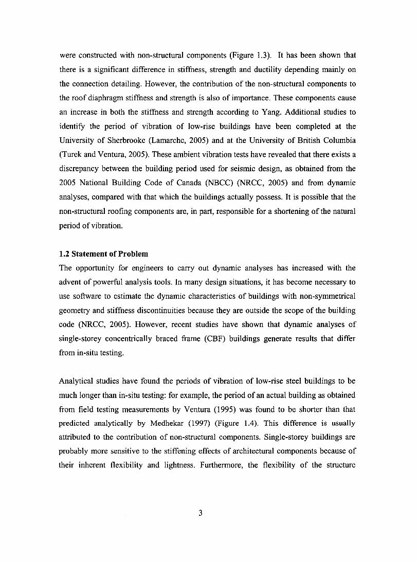
Analytical studies have found the periods of vibration of low-rise steel buildings to be
much longer than in-situ testing: for example, the period of an actual building as obtained
from field testing measurements by Ventura (1995) was found to be shorter than that
predicted analytically by Medhekar (1997) (Figure 1.4). This difference is usually
attributed to the contribution of non-structural components. Single-storey buildings are
probably more sensitive to the stiffening effects of architectural components because of
their inherent flexibility and lightness. Furthermore, the flexibility of the structure
3
originates largely from the roof diaphragm. Medhekar and Yang have shown that non
structural roofing components reduce diaphragm flexibility.
Furthermore, in the NBCC, the magnitude of the seismic loads at a given site depends on
the fundamental period of vibration of the structure, which is often estimated using the
empirical equations that are provided in the building code. These equations have typically
been derived for multi-Ievel buildings with rigid floor and roof diaphragms; therefore
they do not necessarily represent the behaviour of low-rise steel buildings with flexible
roof diaphragms.
At this stage, there remains doubt as to the ability of an engineer to accurately predict the
fundamental period of vibration of a low-rise steel building, and hence to determine
appropriate seismic loads, because of the influence of flexible roof deck diaphragms and
non-structural components.
1.3 Objectives
c o
:;::: ~ CI)
Qi (.) (.)
<C E -(.) CI) c.
ri)
/ Ambient Vibration Measurement
Computed l' Period
Period
Figure 1.4: Periods of vibration
The overall goal of this research is to provide a better understanding of the effect of non
structural roofing components on the performance of single-storey steel buildings
subjected to seismic loading.
The project can be divided into a series of specifie objectives as listed below:
4
a) Determine the material properties for the non-structural roofing components, such
as gypsum board and fibreboard, from ASTM standard laboratory tests.
b) Determine the increase in shear stiffness of the diaphragm due to the non
structural roofing materials, adhered together with hot bitumen.
c) Determine the connection properties between the non-structural roofing materials
and the steel deck diaphragm, as well as the connection stiffness for deck-to
frame and sidelap connections for different deck thicknesses.
d) Develop a linear elastic finite element model of a roof deck diaphragm that
accounts for both the steel panels and non-structural components.
e) Compare the analytical results with the findings of Yang (2003) and Essa et al.
(2001) and stiffness values obtained with the Steel Deck Institute (SDI) equations.
Using the model, carry out a parametric study of diaphragm systems with
different deck thickness and connection patterns to establish the contribution of
the non-structural elements to initial shear stiffness.
1.4 Scope and Limitation of Study
The scope of this project is limited to the materials typically used in the construction of
roof deck diaphragms in Canada. The non-structural roofing components are those used
in the construction of an AMCQ SBS-34 roof as tested by Yang. The gypsum board is
12.7 mm (11") type X, produced by CGC under the brand name Sheetrock, and the
fibreboard is Cascade Securpan 1". The steel roof deck panels specified for study were
those most commonly found in Canada. Four thicknesses of a 38 mm deep deck were
considered: 0.76 mm, 0.91 mm, 1.22 mm and 1.51 mm. The deck-to-frame fasteners were
Hilti X-EDNK-22 THQ 12M powder actuated nails. The gypsum-to-deck connectors
used were SFS intec #12 hex with round ga/va/ume plates, produced under the
Deckfast™ trademark. Hilti S-MD 12-14 X 1 HWH #1 screws were used for the sidelap
connections.
The SAP2000 finite element model was developed to reproduce the diaphragm tests,
3658 mm wide by 6096 mm long (12' X 20'), conducted by Yang, Essa and Martin.
Analyses of the model were conducted in order to obtain the initiallinear elastic response
5

of the roof deck diaphragm as opposed to the inelastic performance as studied by Essa,
Martin and Yang. Furthermore, the SDI design method for deck diaphragm stiffness
(1991) was used to evaluate the stiffness of models for which no test results existed.
1.5 Thesis Outline
This thesis is concemed with the contribution of non-structural components to roof
diaphragm shear stiffness in single-storey concentrically braced frame (CBF) steel
structures. It is divided into three main parts:
Chapter 2 is a review of previously completed research on roof diaphragm behaviour and
on dynamics of low-rise steel buildings.
Chapter 3 focuses on the experimental programs conducted to identify the material
properties of the non-structural roofing components, as weIl as the stiffness of the
diaphragm connections.
Chapter 4 describes the development of the finite element model and the numerical
analyses of roof deck diaphragms with and without non-structural components. A
comparison of the analytical results with the full-scaie diaphragm tests conducted by
Yang (2003) and Essa et al. (2001), as weIl as with the computed SDI values is also
provided. A parametric study of the contribution to shear stiffness of non-structural
components is also carried out, for which various diaphragm configurations are
considered.
Chapter 5 lists the conclusions of the study and highlights recommendations for further
research in this field.
6
2.1 General
CHAPTER2
LITERA TURE REVIEW
Johnson and Converse (1947) were the first to carry out the testing of cold fonned steel
diaphragms. Since then, an important and large body of work has been compiled. This
Chapter will review sorne of the research on cold fonned steel deck diaphragms that has
been completed over the years. Emphasis is placed on the previous studies by Rogers and
Tremblay (2000, 2003a,b), Essa et al. (2001,2003), Martin (2002) and Yang (2003) that
fonn the initial phases of the single-storey steel structure / flexible roof diaphragm
research project at École Polytechnique and McGill University.
2.2 Nilson
Nilson's publication "Shear Diaphragms of Light Gage Steel" (1960) was the first
substantial test pro gram on steel deck diaphragms. He developed two test approaches
(cantilever and simple beam) that are still used by researchers to this day. Both test setups
are now inc1uded in the ASTM E455 (2002) Standard.
Nilson carried out 39 monotonie tests of bare sheet steel diaphragms. He wrote that
"diaphragm strength of floor and roof elements can be utilized to resist horizontaUy
applied /oads" and "be effective as shear diaphragms". However, Nilson dec1ared that
the analysis of steel deck diaphragms is not feasible, as it is made up of many small parts
and stress concentrations at the welded connections. He also suggested using the
cantilever test frame rather than the simple beam. Nilson conc1uded that full-scale tests
are still the most reliable method to evaluate diaphragm behaviour.
2.3 Luttrell
Luttrell has been involved in the study of steel deck diaphragm design since the sixties
and has been technical advisor to the Steel Deck Institute (SDI) since 1965. A large
proportion of his research has been the testing of roof deck diaphragms and their
connections, from which he derived the SDI design method for light gauge steel roof
diaphragms (SDL 1981, 1991). The SDI method is commonly used by structural
7
engineers in North America for the design of diaphragms. The overall in-plane shear
stiffness of a bare sheet steel diaphragm depends on the type of panel, the number of
panels, the number of fasteners per panel, the stiffness of the fasteners (both deck-to
frame and sidelap), as well as the dimensions of the diaphragm. For a full review of the
SDI design method by Luttrell the reader is referred to the thesis ofNedisan (2002).
Luttrell also mentions that non-structural members may increase in-plane shear stiffness
and strength. He states that "systematic attachment of rigid fiat panels to the top
corrugations of a diaphragm can increase both diaphragm strength and stiffness. {. . .]
Properly located attachments through the panels and into the tops of the deck
corrugation, particularly on the diaphragm perimeter, limit warping and increase shear
stiffness" (Luttrell, 1995).
2.4 Tremblay and Stiemer
The non-linear response of 36 rectangular single-storey steel buildings subjected to
historical earthquake ground motion records was examined by Tremblay and Stiemer
(1996). The lateral load resisting systems of these structures were made up of a flexible
metal roof diaphragm and vertical bracing located along the exterior walls. Periods of
vibration of these buildings were computed firstly by assuming that the roof diaphragm
was perfectly rigid and secondly, by assuming that a flexible roof diaphragm existed.
Tremblay and Stiemer noted that the influence of the diaphragm is very clear: the period
of vibration of the structures increased dramatically. The period of vibration, when
accounting for the flexible diaphragm, was on average 1.5 times longer than with a rigid
diaphragm in the short direction of the building, and between 2 and 3 times longer in the
other direction. The study showed that diaphragm flexibility influenced the overall lateral
stiffness of a structure, and hence, should be taken into account when computing the
period of vibration of steel single-storey buildings.
2.5 Medhekar
Medhekar' s thesis entitled "Seismic evaluation of steel building with concentrically
braced frames" contained the findings of an investigation into the behaviour of single-
8

storey and two-storey steel buildings with concentrically braced frames (CBFs) designed
according to the 1995 NBCC (NRCC, 1995) provisions and the SI6.1-94 Standard (CSA,
1994). Medhekar also reviewed a seismic design method based on displacement limits
rather than force limits (Medhekar, 1997; Medhekar and Kennedy, 1999).
His study of single-storey CBF steel buildings showed that the roof diaphragm flexibility
has a significant impact on the overall period of vibration of the building. Based on
Medhekar's work, Tremblay et al. (2000) established the following equations to
determine the period based on a combination of the bracing and diaphragm stiffness:
where:
where:
KB = lateralload resisting system (LLRS) stiffness,
KD = roof diaphragm stiffness,
W = seismic weight,
L = length of roof diaphragm,
G ' = roof diaphragm shear stiffness,
E = modulus of elasticity of steel deck,
1 = steel deck equivalent inertia,
b = diaphragm width.
(2-1)
(2-2)
Furthermore, Medhekar accounted for the contribution of non-structural components to
overall building stiffness, and more specifically, included the shear stiffness of the
gypsum board to the in-plane roof diaphragm shear stiffness. He evaluated the in-plane
shear stiffness of the gypsum board to be 1.1 kN/mm. This value was based on a tangent
modulus of rigidity of 69 MPa.
9
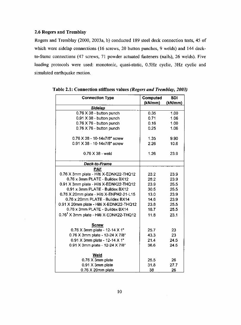
2.6 Rogers and Tremblay
Rogers and Tremblay (2000, 2003a, b) conducted 189 steel deck connection tests, 45 of
which were sidelap connections (16 screws, 20 button punches, 9 welds) and 144 deck
to-frame connections (47 screws, 71 powder actuated fasteners (nails), 26 welds). Five
loading protocols were used: monotonic, quasi-static, 0.5Hz cycIic, 3Hz cycIic and
simulated earthquake motion.
Table 2.1: Connection stiffness values (Rogers and Tremblay, 2003)
Connection Type Computed SOI (kN/mm) (kN/mm)
Side/ap 0.76 X 38 - butlon punch 0.35 1.00 0.91 X 38 - butlon punch 0.71 1.06 0.76 X 76 - butlon punch 0.16 1.00 0.76 X 76 - butlon punch 0.25 1.06
0.76 X 38 - 10-14x7/8" screw 1.35 9.90 0.91 X 38 -10-14x7/8" screw 2.26 10.6
0.76 X 38 - weld 1.26 23.9
Deck-to-Frame PAF
0.76 X 3mm plate - Hilti X-EDNK22-THQ12 23.2 23.9 0.76 x 3mm PLATE - Buildex BX12 28.2 23.9
0.91 X 3mm plate - Hilti X-EDNK22-THQ12 23.9 25.5 0.91 x 3mm PLATE - Buildex BX12 30.5 25.5
0.76 X 20mm plate - Hilti X-ENPH2-21-L 15 13.0 23.9 0.76 x 20mm PLATE - Buildex BX14 14.6 23.9
0.91 X 20mm plate - Hilti X-EDNK22-THQ12 23.8 25.5 0.76 x 3mm PLATE - Buildex BX14 18.7 25.5
0.761 X 3mm plate - Hilti X-EDNK22-THQ12 11.8 23.1
Screw 0.76 X 3mm plate - 12-14 X 1" 25.7 23
0.76 X 3mm plate - 12-24 X 7/8" 43.3 23 0.91 X 3mm plate - 12-14 X 1" 21.4 24.5
0.91 X 3mm plate - 12-24 X 7/8" 36.6 24.5
Weld 0.76 X 3mm plate 25.5 26 0.91 X 3mm plate 31.8 27.7
0.76 X 20mm plate 38 26
10

The obtained data revealed that the type of fastener influences the ultimate capacity,
stiffness and energy dissipating characteristics ofthe connection. For sidelaps, the welded
connections could absorb the greatest amount of energy, followed by button punched
connections and finally screwed connections. For the deck-to-frame connections, the
nailed connections proved to be the most effective energy dissipating connector, followed
closely by the screwed connections. The welded connections showed significant ultimate
capacities but very low ductility, failing at small displacements when subjected to
repeated loads, thus exhibiting low energy dissipation.
The data obtained from these tests is critical in the building of a finite element model that
will accurately recreate the actual behaviour of steel deck roof diaphragms. Although
tests were performed on connection specimens for this research project, this data was
used to build preliminary models. Sorne of the values obtained from their tests are
presented in Table 2.1.
2.7 Essa et al.
The main objective of the research pro gram was to investigate the overall behaviour of
the shear diaphragm, focussing on the energy dissipating capability, ductility, stiffness
and ultimate capacity. Other than overall behaviour of the diaphragm, connection
stiffness was also investigated: comparisons of SDI (1991) and CSSBI (1991) diaphragm
strength, Su, and shear stiffness, G' as defined previously, predictions were made with test
based values (Essa et al., 2001, 2003).
Eighteen full-scale (3.66 x 6.09 m) cantilever bare steel diaphragm tests were conducted:
16 of which were constructed of 0.76 mm panels and 2 with 0.91 mm panels. Both
standard (interlock) and B-deck (nestable) panels with a 38 mm deep profile were used.
A variety of connections were placed; for sidelap connectors, welded, button punched
and screwed connections were installed and for the deck-to-frame connectors, welds,
welds with washer, screws and nails were used. Of each connection configuration, two
specimens were tested: one loaded monotonically and the other with a quasi-static
reversed cyclic load protocol.
11
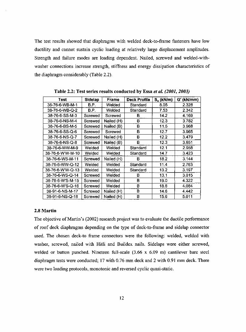
The test results showed that diaphragms with welded deck-to-frame fasteners have low
ductility and cannot sustain cyclic loading at relatively large displacement amplitudes.
Strength and failure modes are loading dependent. Nailed, screwed and welded-with
washer connections increase strength, stiffness and energy dissipation characteristics of
the diaphragm considerably (Table 2.2).
Table 2.2: Test series results conducted by Essa et al. (1001, 1003)
Test Sidelap Frame Deck Profile Su (kN/m) G' (kN/mm) 38-76-6-W8-M-1 8.P. Welded Standard 8.05 2.328 38-76-6-W8-Q-2 8.P. Welded Standard 7.53 2.342 38-76-6-SS-M-3 Screwed Screwed 8 14.2 4.169 38-76-6-NS-M-4 Screwed Nailed (H) 8 12.3 3.782 38-76-6-8S-M-5 Screwed Nailed (8) 8 11.5 3.968 38-76-6-SS-Q-6 Screwed Screwed 8 12.7 3.965 38-76-6-NS-Q-7 Screwed Nailed (H) 8 12.2 3.479 38-76-6-NS-Q-8 Screwed Nailed (8) 8 12.3 3.651
38-76-6-WW-M-9 Welded Welded Standard 12.1 2.958 38-76-6-W'W-M-10 Welded Welded Standard 14.7 3.423 38-76-6-WS-M-11 Screwed Nailed (H) 8 18.2 3.144
38-76-6-WW-Q-12 Welded Welded Standard 11.4 2.763 38-76-6-W'W-Q-13 Welded Welded Standard 13.2 3.197 38-76-6-WS-Q-14 Screwed Welded 8 13.1 3.015 38-76-6-W'S-M-15 Screwed Welded 8 19.0 4.322 38-76-6-W'S-Q-16 Screwed Welded 8 18.8 4.084 38-91-6-NS-M-17 Screwed Nailed (H) 8 14.6 4.442 38-91-6-NS-Q-18 Screwed Nailed (H) 8 15.6 5.011
2.8 Martin
The objective of Martin's (2002) research project was to evaluate the ductile performance
of roof deck diaphragms depending on the type of deck-to-frame and sidelap connector
used. The chosen deck-to frame connectors were the following: welded, welded with
washer, screwed, nailed with Hitli and Buildex nails. Sidelaps were either screwed,
welded or button punched. Nineteen full-scale (3.66 x 6.09 m) cantilever bare steel
diaphragm tests were conducted; 17 with 0.76 mm deck and 2 with 0.91 mm deck. There
were two loading protocols, monotonie and reversed cyclic quasi-static.
12

The experimental data showed that roof diaphragms made with button punched sidelap
and welded deck-to-frame connections must remain in the elastic range to resist seismic
loading. However, roof diaphragms with nailed deck-to-frame connections and screwed
sidelaps can undergo inelastic deformation while maintaining enough capacity to resist
the seismic loads. The results of the tests conducted by Martin are shown in Table 2.3.
Table 2.3: Large-scale diaphragm test series by Martin (2002)
Test Sidelap Frame Deck Su G' Profile (kN/m) (kN/mm)
38-91-6-N S-M-19 Screwed Nailed (H) (1) B 16.7 4.13
38-76-6-WB-SD-20 B.P. Welded (2) Standard 9.81 2.44
38-91-6-WB-SD-21 B.P. Welded (2) Standard 13.8 3.16
38-91-6-W'W-M-22 W.W.W.(3) W.W. washer (4) B 32.1 4.54
38-91-6-W'W-SD-23 W.W.W.(3) W.W. washer (4) B 34.6 4.60
38-91-6-W'W-LD-24 W.W.W.(3) W.W. washer (4) B 33.2 4.36
38-91-6-NW-M-25 W.W.W.(3) Nailed (H) (5) B 22.5 4.33
38-91-6-NW-SD-26 W.W.W.(3) Nailed (H) (5) B 26.5 4.09
38-91-6-NW-LD-27 W.W.W.(3) Nailed (H) (5) B 26.2 3.64
38-76-6-NS-SD-28 Screwed Nailed (H) (1) B 14.1 2.45
38-76-6-NS-LD-29 Screwed Nailed (H) (1) B 13.6 2.37
38-76-6-NS-M-30 (6) Screwed Nailed (H) (1) B 23.4 13.5
38-76-6-NS-SD-31 (6) Screwed Nailed (H) (1) B 26.5 15.0
38-76-6-NS-LD-32 (6) Screwed Nailed (H) (1) B 34.4 18.3
38-91-6-NS-SD-33 (6) Screwed Nailed (H) (1) B 35.2 18.4
38-91-6-NS-SD-34 Screwed Nailed (H) (1) B 17.0 4.01
38-91-6-NS-LD-35 Screwed Nailed (H) (1) B 17.3 3.90
38-76-6-WB-SD-36 B.P. Welded (2) Standard 5.80\ta) 2.40\fa) 5.69(7b) 0.94(7b)
38-91-6-WB-M-37 B.P. Welded (2) Standard 12.6 3.32 (1): Used Hilb (H) X-EDNK22-THQ12 fastener for nailed frame connection and 12-14-7/8" fastener for screwed sidelap connections. (2): Welded frame connections were made with 16 mm diameter arc spot welds. (3): Welded sidelap connection with washers (4);: Welded frame connections with washers. (5): Used Hilti (H) X-EDNK22-THQ12 fastener for nailed frame connections. (6): AlI fasteners spaced at 152 mm ole in both directions, spacing in aIl others tests equal to 305 mm. (7): 200 cycles at 0.4 'Yu (a) and 2 cycles at 0.6 'Yu (b) prior to short duration loading protocol.
Martin looked at the inelastic performance of the seismic force resisting system when the
diaphragm was selected as the energy dissipating element by means of dynamic analyses
with the software Ruaumoko (Carr, 2000). He showed that only certain connection
13
configurations (nail & screw) could be relied on to obtain the ductility needed to specify
force modification factors greater than one for seismic design. However, the diaphragm
element used in the non-linear time history dynamic analyses was calibrated from the
results of the tests by Essa et al .. No account of the effect of the non-structural roofing
components was made.
2.9 Nedisan
The objective of this project was to conduct numerical analyses of single-storey steel
buildings with flexible diaphragms (Nedisan, 2002). The first stage of this project was to
develop a better understanding of the SDI equations for the calculation of roof diaphragm
stiffness and strength. As a second stage, periods of vibration were calculated for
structures using three methods: a DRAIN-2D analysis model, the formula developed by
Medhekar (1997) and the FEMA273 (1994) equation. AIl methods gave similar results
for six buildings, while using both the 1995 NBCC and the 2005 NBCC (NRCC, 2005).
Nedisan, using the equations developed by Medhekar (1997), then calculated periods of
vibration of buildings and compared the values obtained to shake table tests conducted by
Tremblay and Bérair (1999). The results obtained by the equations were very similar to
the test results obtained by Medhekar.
2.10 Yang
Yang (2003) conducted 12 large-scale roof diaphragm tests under both monotonic and
reversed cyclic quasi-static loading. A total of 10 specimens consisted of bare steel roof
deck; however two of the diaphragms were constructed with the non-structural roofing
components. Roof construction can vary significantly from one project to another, thus
after conducting an extensive literature review and consulting with the Ontario Industrial
Roofing Contractors Association (OIRCA) and the Association des Maîtres Couvreurs.du
Québec (AMCQ), the AMCQ SBS-34 roofing system was chosen. It is a common and
conventional system composed of the following layers:
• Two layers (4 mm + 2.2 mm) ofSBS waterproof membrane;
14

• One layer of25 mm (1") thick 1219.2 mm by 1219.2 mm (4'x4') non-flammable
wood fibreboard, hot bitumen adhered;
• One layer of 63.5 mm (2.5") thick polyisocyanurate (ISO) insulation, hot bitumen
adhered;
• Two layers of paper vapour retarder (No. 15 asphalted felts), hot bitumen
adhered;
• One layer of 12.7 mm (12") thick 1219.2 mm by 2438.4 mm (4'x8') type X
gypsum board, 12 screws per panel mechanically fastened;
• Steel deck.
The bitumen used was Type 2 asphalt conforming to CSA A123.4 (Baker, 1980). A
cross-section of the final roof diaphragm specimen tested by Yang is shown in Figure 2.1.
Fibreboard
+--ISO board
board
Figure 2.1: Roof cross-section tested by Yang (2003)
Test specimens were constructed with various connection detailing, end lap conditions,
loading and deck thickness / height. The deck-to-frame connectors consisted of Buildex
powder actuated fasteners, Hilti powder actuated fasteners or welds. The sidelap
connections consisted of screwed fasteners (Hilti or Buildex screws) or button punches.
15
Three loading protocols were used: monotonic, seismic short duration loading or a cyclic
load protocol foHowed by a monotonic loading.
The test specimens were divided into four groups. Group 1 consisted of a single test,
specimen 38, which had screwed sidelap connections, Buildex powder actuated fasteners
(PAF) for the deck-to-frame connectors and P3615-B 0.91 mm thick steel deck. It
underwent the short duration seismic loading developed by Martin (2002), which lasts 25
seconds.
Group 2 contained four test specimens, tests 39 to 42. The defining characteristic was that
there was a longitudinal overlap at the mid-point of the specimens. Two specimens had
screwed sidelap connections and Hilti PAF deck-to-frame connections. The first of the
two was tested with a monotonie loading protocol; the second with a short duration
seismic loading protocol. The two others had button punched sidelap connections and
welded deck-to-frame connections. As with the two previous specimens in Group 2, the
first specimen was loaded monotonicaHy and the second underwent a short duration
seismic loading protocol. AH specimens were constructed with P3615-B 0.76 mm steel
deck.
Tests 43 to 46 made up Group 3. AH tests had screwed sidelap connectors and Hilti PAFs
for the deck-to-frame connectors and used a P3615-B 0.76 mm sheet steel deck. Tests 43
and 44 were bare sheet steel, whereas tests 45 and 46 had the non-structural roofing
components added. Tests 43 and 45 were loaded monotonicaHy and tests 44 and 46 were
loaded using a cyclic loading protocol foHowed by a monotonie loading. These tests were
done in order to determine the contribution of the non-structural components to overaH
in-plane strength and stiffness.
The three final tests were compiled in Group 4. AH were button punched for sidelap and
aH had welded deck-to-frame connections. Tests 47 and 48 had P2436 0.76 mm deck
whereas test 49 was made of P2436 0.91 mm deck. Tests 47 and 49 were tested with a
16
monotonic load protocol, while specimen 48 was tested with a short duration seismic
loading protocol.
The main topic of research was the inelastic behaviour of steel roof deck diaphragms. In
testing, it was found that the non-structural components, if appropriately fastened to the
steel roof deck, increased both the in-plane shear strength and stiffness of the diaphragm.
In this test model, gypsum board fastened by screws to the steel deck was found to
influence the diaphragm properties to the greatest extent. An increase of the mean
strength of approximately 26% was realised, in addition to a mean stiffness increase of
near 46% for the tested diaphragms.
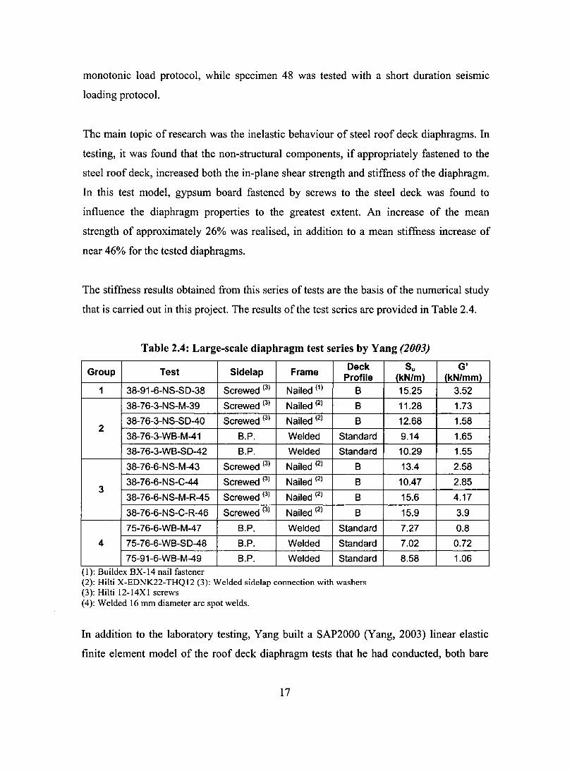
The stiffness results obtained from this series of tests are the basis of the numerical study
that is carried out in this project. The results of the test series are provided in Table 2.4.
Table 2.4: Large-scale diaphragm test series by Yang (2003)
Group Test Sidelap Frame Oeck
Profile 1 38-91-6-NS-SD-38 Screwed (3) Nailed (1) B
38-76-3-NS-M-39 Screwed (3) Nailed (2) B
38-76-3-NS-SD-40 2
Screwed (3) Nailed (2) B
38-76-3-WB-M-41 B.P. Welded Standard
38-76-3-WB-SD-42 B.P. Welded Standard
38-76-6-NS-M-43 Screwed (3) Nailed (2) B
38-76-6-NS-C-44 Screwed (3) Nailed (2) B 3
38-76-6-NS-M-R-45 Screwed (3) Nailed (2) B
38-76-6-NS-C-R-46 Screwed (3) Nailed (2) B
75-76-6-WB-M-47 B.P. Welded Standard
4 75-76-6-WB-SD-48 B.P. Welded Standard
75-91-6-WB-M-49 B.P. Welded Standard (1): Buildex BX-14 nail fastener (2): Hilti X-EDNK22-THQ12 (3): Welded sidelap connection with washers (3): Hilti 12-14X1 screws (4): Welded 16 mm diameter arc spot welds.
Su (kN/m)
15.25
11.28
12.68
9.14
10.29
13.4
10.47
15.6
15.9
7.27
7.02
8.58
G' ~kN/mml
3.52
1.73
1.58
1.65
1.55
2.58
2.85
4.17
3.9
0.8
0.72
1.06
In addition to the laboratory testing, Yang built a SAP2000 (Yang, 2003) linear elastic
finite element model of the roof deck diaphragm tests that he had conducted, both bare
17

steel and clad versions (Figure 2.2). The model was 914.4 mm wide by 3048 mm long,
representing a single width of roof deck that was half as long as the actual diaphragm test
specimen. A cantilever analysis mode1 was selected in an attempt to adequately recreate
the test conditions. Yang built models with different numbers of elements, dividing the
deck into 500, 1596 and 3192 elements, to identify the effect of the finite element mesh.
The gypsum board was also divided into firstly 40 shell elements and was later divided in
1596 shell elements. The linear elastic model was able to adequately recreate the warping
that the cross-section underwent under loading; as well, the results obtained became more
accurate as the number of shell elements was increased. The 1596 element model was
deemed sufficient to obtain outputs that were consistent with the experimental results.
For the model that included the non-structural components, the stiffness of the gypsum
was unknown at that point. Three values were assumed for flexural stiffness: 2.0 GPa, 1.0
GPa, and 0.293 GPa and Poisson's ratio was chosen to be 0.3. With respect to
connection stiffuess, values were taken from Rogers and Tremblay (2000, 2003a,b) for
both the sidelap and deck-to-frame connectors.
Figure 2.2: Underformed shapes ofbare sheet steel deck (left) and deck with
gypsum elements (right) (Yang, 2003).
The results of the linear elastic analyses conducted by Yang are presented in Table 2.5.
Based on test results the desired values were 2.58 kN/mm for the bare sheet steel and
4.17 kN/mm for the model with the roofing components. As can be seen, Yang was not
able to precisely replicate the measured stiffness of the test diaphragms using the finite
element analyses. The 1592 shell element model is an adequate mesh density as the
18
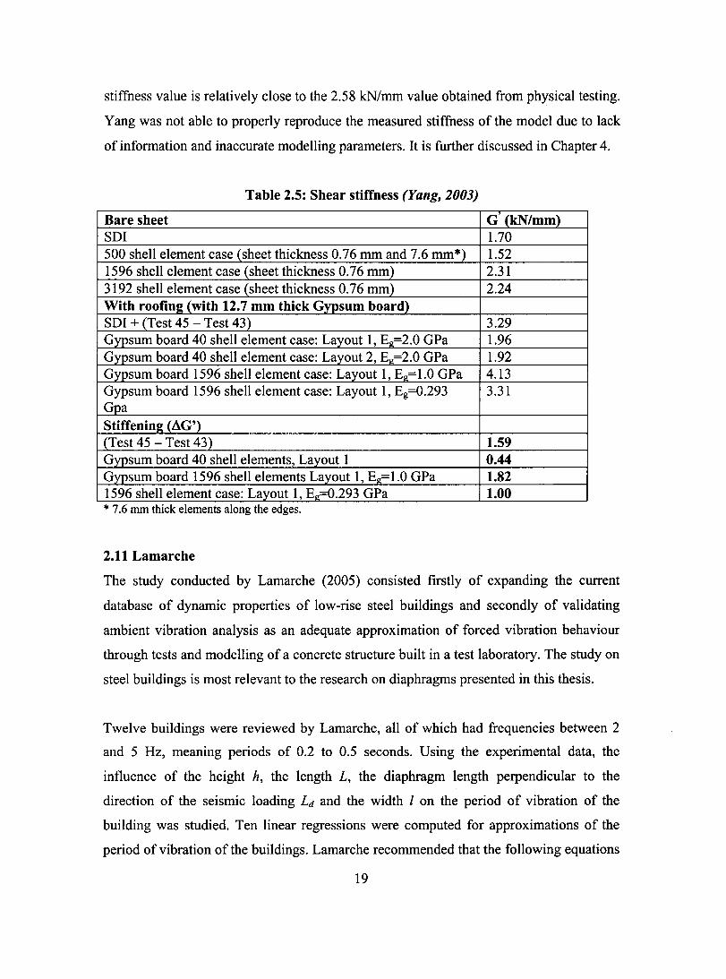
stiffness value is relatively close to the 2.58 kN/mm value obtained from physical testing.
Yang was not able to properly reproduce the measured stiffness of the model due to lack
of information and inaccurate modelling parameters. It is further discussed in Chapter 4.
Table 2.5: Shear stiffness (Yang, 2003)
Bare sheet G (kN/mm) SDI 1.70 500 shen element case (sheet thickness 0.76 mm and 7.6 mm*) 1.52 1596 shen element case (sheet thickness 0.76 mm) 2.31 3192 shen element case (sheet thickness 0.76 mm) 2.24 With rooting (with 12.7 mm thick Gypsum board) SDI + (Test 45 - Test 43) 3.29 Gypsum board 40 shen element case: Layout 1, Eg=2.0 GPa 1.96 Gypsum board 40 shen element case: Layout 2, Eg=2.0 GPa 1.92 Gypsum board 1596 shen element case: Layout 1, EI!=1.0 GPa 4.13 Gypsum board 1596 shen element case: Layout 1, Eg=0.293 3.31 Gpa Stiffening (AG') (Test 45 - Test 43) 1.59 Gypsum board 40 shen elements, Layout 1 0.44 Gypsum board 1596 shen elements Layout 1, EI!= 1.0 GPa 1.82 1596 shen element case: Layout 1, Eg=0.293 GPa 1.00 * 7.6 mm thick elements along the edges.
2.11 Lamarche
The study conducted by Lamarche (2005) consisted firstly of expanding the CUITent
database of dynamic properties of low-rise steel buildings and secondly of validating
ambient vibration analysis as an adequate approximation of forced vibration behaviour
through tests and modelling of a concrete structure built in a test laboratory. The study on
steel buildings is most relevant to the research on diaphragms presented in this thesis.
Twelve buildings were reviewed by Lamarche, an of which had frequencies between 2
and 5 Hz, meaning periods of 0.2 to 0.5 seconds. Using the experimental data, the
influence of the height h, the length L, the diaphragm length perpendicular to the
direction of the seismic loading Ld and the width 1 on the period of vibration of the
building was studied. Ten linear regressions were computed for approximations of the
period of vibration of the buildings. Lamarche recommended that the fonowing equations
19
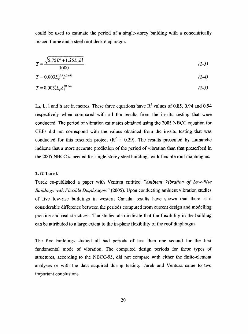
could be used to estimate the period of a single-storey building with a concentrically
braced frame and a steel roof deck diaphragm.
~5.75L2 + 1.25Ld hl T = -'--------'--
1000
T = 0.003L~75 hO.675
(2-3)
(2-4)
(2-5)
Ld, L,land h are in metres. These three equations have R2 values of 0.85, 0.94 and 0.94
respectively when compared with aIl the results from the in-situ testing that were
conducted. The period of vibration estimates obtained using the 2005 NBCC equation for
CBFs did not correspond with the values obtained from the in-situ testing that was
conducted for this research project (R2 = 0.29). The results presented by Lamarche
indicate that a more accurate prediction of the period of vibration than that prescribed in
the 2005 NBCC is needed for single-storey steel buildings with flexible roof diaphragms.
2.12 Turek
Turek co-published a paper with Ventura entitled "Ambient Vibration of Low-Rise
Buildings with Flexible Diaphragms" (2005). Upon conducting ambient vibration studies
of five low-rise buildings in western Canada, results have shown that there is a
considerable difference between the periods computed from current design and modelling
practice and real structures. The studies also indicate that the flexibility in the building
can be attributed to a large extent to the in-plane flexibility of the roof diaphragm.
The five buildings studied aIl had periods of less than one second for the first
fundamental mode of vibration. The computed design periods for these types of
structures, according to the NBCC-95, did not compare with either the finite-element
analyses or with the data acquired during testing. Turek and Ventura came to two
important conclusions.
20
For the three steel buildings that were tested, the periods of vibration ranged from 0.25 to
0.9 seconds, although they were aIl of similar height. This suggests that computing the
period of vibration based on height al one is not adequate for low-rise steel structures.
Furthermore, the mode shapes that were obtained showed that there is a significant
amount of flexibility in the roof diaphragm. These two conclusions suggest that the
current design methods for low-rise steel buildings are not adequate, as they do not
reproduce the actual dynamic behaviour of these structures.
2.13 2005 NBCC
The 2005 National Building Code of Canada (NBCC) (NRCC, 2005) is the model code
that will be used throughout Canada, in part, to estimate the loads that act on structures.
The sei smic provisions in this document declare that:
"Structures shall be designed with a clearly defined load path, or paths, to transfer the
inertia forces generated in an earthquake to the supporting ground. The structures shall
have a clearly defined Seismic Force Resisting System(s) (SFRS). The SFRS shall be
designed to resist 100% of the earthquake loads and their effects, other structural
framing elements not considered to be part of the SFRS must keep elastic, or have
sufficient nonlinear capacity to support both gravity loads and earthquake effects. "
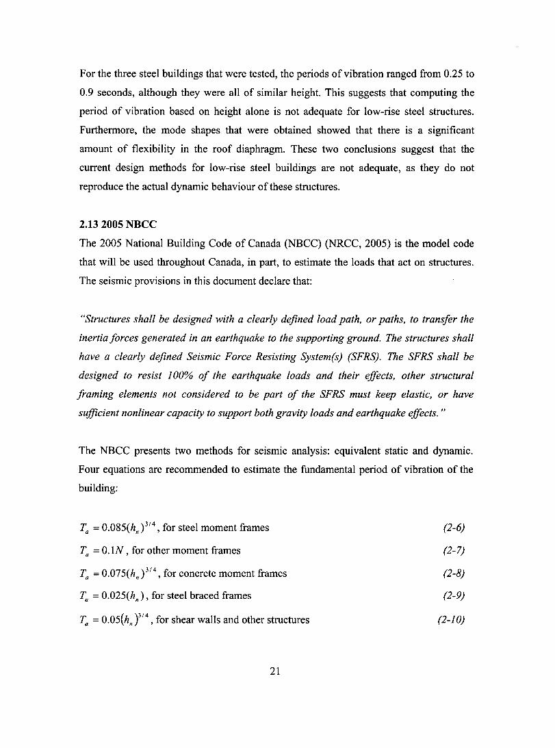
The NBCC presents two methods for seismic analysis: equivalent static and dynamic.
Four equations are recommended to estimate the fundamental period of vibration of the
building:
Ta = 0.085(hn )3/4 , for steel moment frames
Ta = O.lN , for other moment frames
Ta = 0.075(hn )3/4, for concrete moment frames
Ta = 0.025(hn ) , for steel braced frames
( )3/4
Ta = 0.05 hn , for shear waIls and other structures
21
(2-6)
(2-7)
(2-8)
(2-9)
(2-10)

In the above equations, hn is the height in metres of the building above ground level and
N in Eq. 2-7 is the total number of storeys. Equation 2.9 is used for single-storey
concentrically braced frame (CBF) steel buildings. If dynamic analyses or other means
are used to determine the value of Ta for a particular building, then the value must not be
greater than two times the result ofEq. 2-9 for the CBF seismic force resisting system.
These equations were developed for multi-storey buildings. It has been shown that they
do not adequately recreate single-storey steel building dynamic behaviour, mainly due to
the fact that the diaphragm flexibility is not accounted for (Tremblay, 2005). If Eq. 2-9 is
used to compute the period of vibration of CBF buildings, the values obtained do not
correspond to those measured by in-situ testing that was completed at the University of
British Columbia (Ventura and Turek, 2005) and at the Université de Sherbrooke
(Lamarche, 2005).
2.14 C8A 816
Clause 27 of the CSA S16 Standard (2001) provides for the seismic design of steel
buildings, which is based on a capacity design concept. No specific design information
with regards to roof deck diaphragms is prescribed; rather the S 16 Standard addresses
mainly the design of beams, columns, braces and common frames subjected to seismic
loads. However, it is stated that all members in the seismic force resisting system except
the weak link element must be capable of resisting the full seismic load. Only the chosen
element, typically the brace in CBFs, is allowed to reach the inelastic range. It also states
that the diaphragm and "collector elements are capable of transmitting the loads
developed at each level to the vertical lateral-load-resisting system." This obviously also
applies to roof deck diaphragms.
However, there is sorne flexibility in the requirements of the S 16 Standard. Clause 27.11
states that "Other framing systems and frames that incorporate [ ... ] other energy
dissipating devices shall be designed on the basis of published research results or design
guides, observed performance in past earthquakes, or special investigation. " Therefore,
22
the use of the roof deck diaphragm as the weak element, although not discussed in S 16, is
possible if justified through appropriate research and testing.
2.15 Summary
The behaviour of bare sheet steel roof deck diaphragms has been extensively studied. In
contrast, tests of only two diaphragms with non-structural components have been
conducted (Yang, 2003). It has been shown that these additional roofing components
result in a significant increase in both strength and stiffness of the diaphragm. In addition,
recent studies by Medhekar, Tremblay & Steimer, Lamarche as weIl as Ventura and
Turek have shown that the flexibility of the clad diaphragm affects the overall building
period. Rence there is a need to identify the impact of non-structural roof diaphragm
components on building behaviour, such that more accurate, and perhaps economic,
seismic designs can be obtained. The FEM study by Yang can be used as a starting point
for the development of a more detailed and larger scale linear elastic diaphragm mode!.
The connection data presented in this Chapter will also be useful in developing finite
element models. Moreover, the results of the large-scale diaphragm tests by Essa et al.,
Martin and Yang will be of significant importance in the calibration of any finite element
model that is developed.
23

CHAPTER3
MATERIAL AND CONNECTION EXPERIMENTS
3.1 General
The objective of the experimental phase of this research project was to determine the
material properties of the non-structural roofing components and their connections. These
properties are not readily available in the literature, and hence, physical testing was
necessary. The resulting material properties were needed for the development of the finite
element models described in Chapter 4. A total of four different test setups were used for
this research. The first is a simple two-sided shear test in which the shear stiffness of the
gypsum and fibreboard can be measured on a local scale (Section 3.2). The second test
setup is a centre point load flexural test, which was necessary to determine the flexural
stiffness of the gypsum and fibreboard (Section 3.3). The third test is a four-sided shear
test, for which the shear stiffness of the gypsum, fibre board and combinations of other
roofing components were measured (Section 3.4). It was the most complex of aIl setups,
but was necessary because of the type and size of roofing components. The final test
setup was of the screw connection between the gypsum and underlying steel deck, as weIl
as the screw sidelap connections and nailed deck-to-frame connections. In Section 3.5 a
discussion ofhow the stiffness values were determined for this connection type, and their
values, is presented. Each of the test setups will be described in detail; the size and shape
of tested specimens, test frame geometry and construction, testing protocol, material
combinations and results will be provided. In addition, the preliminary conclusions for aIl
of the experimental results are provided in Section 3.6.
The non-structural components remain constant throughout this chapter: the fibreboard is
Cascade Securpan 1" and the gypsum board is CGC Type X W'.
3.2 Two-Sided Shear Test
3.2.1 Setup and Test Procedure
The two-sided shear test was conducted in order to obtain shear stiffness values for the
roofing materials on a local scale. It was carried out in accordance with ASTM DI037
(1999). A similar setup was used by Boudreault (2005) for the testing / evaluation of
24

shear stiffness properties of plywood and oriented strand board (OSB) sheathing. Figure
3.1 shows a photograph of the test setup with a gypsum board specimen, as weIl as a
schematic drawing. The inner surface of the steel loading rails was serrated such that no
slippage would occur under loading when the bolts on each side of the specimen were
tightened. Slippage would compromise the accuracy of the test; in addition it would cause
bearing failure of the specimen against the bolts. This failure mode would result in a
much lower strength and stiffness than if shear failure were to occur along the length of
the specimen. The shear deformation of the specimen was directly measured by an L VDT
placed in line with the loading plates, as shown in Figure 3.1. The steelloading rails are
precisely 25.4 mm (1") apart.
The machine used for this setup was an MTS Sintech 30/G with a 150kN load cell. The
load was applied through a uniform rate of motion of the crosshead of the testing
machine. The rate of loading is taken as 0.2% of the length of the specimen per minute,
that is 0.508 mm/min (0.02 in/min). The L VDT and load cell were connected to a Vishay
Model 5100B scanner, which was used to record the data using the Vishay System 5000
StrainSmart software.
5' r i i
~ __ 1'h·(31.75mm)
Figure 3.1: Two-sided shear setup (Boudreault, 2005)
25
3.2.2 Test Specimens
Test specimens were cut in rectangular sections of254 mm by 88.9 mm (10" by 3.5") as
per the ASTM DI037 Standard. 12.7 mm (12") holes were drilled in order to secure the
specimen properly to the test setup. The specimens were also the full thickness of the
gypsum board (12.7 mm nominal) and the fibreboard (25.5 mm nominal). Furthermore,
according to the ASTM standard, aIl specimens were cut at least four inches from the
panel edges.
Special care was taken when cutting the gypsum board, as it is very brittle and the corners
tend to break. Therefore the gypsum board was cut by knife to slightly larger than
specified, and then the specimen was scraped along its edges with a knife blade until the
size of the specimen was acceptable. Furthermore, the same brittleness caused problems
when the holes were drilled: the paper on the back of the gypsum board tended to rip and
damage the board next to the hole. Therefore, the gypsum board had to be drilled with a
support underneath it, such as a piece of plywood.
The fibreboard was cut on the table saw and with the radial saw. When drilling the
fibre board, the same problem of ripping occurred as with the gypsum board, although this
time, it was caused by the low density of the material. The same method was used to limit
ripping at the back of the specimen.
The thickness of each specimen was measured prior to testing at six different locations on
the specimen. Afterwards, the arithmetic average and the standard deviation were
calculated. The average values were then used to calculate both stiffness and strength
values (Tables 3.1 & 3.2).
A total of six fibreboard specimens and four gypsum board specimens were tested.
However, only five test results are compiled for thefibreboard because the data obtained
from Test 1 was corrupted. A typical gypsum specimen after testing is shown in Figure
3.2.
26
Figure 3.2: Gypsum shear test specimen
3.2.3 Specimen Behaviour
3.2.3.1 Fibreboard
The fibreboard shear specimens behaved linearly up to approximately 40% of the
ultimate load. After this load level a non-linear region existed, that included a significant
decrease in strength once the peak shear load had been attained. Figure 3.3 shows the
shear load versus deformation curve of the fibreboard. In the post-elastic range, Test 2
did not behave in the same manner as the remaining specimens. However, the linear
elastic range of the data was relatively similar for aU tests. Since only these linear elastic
properties were used in the finite element analyses (Chapter 4) the unusual result obtained
for Test 2 after the elastic range did not play a substantial role. However, Test 2 was not
used to compute the average shear strength of the fibreboard.
27

8000 Test 2 --- Test 3
- Test 4 - Test 5
.,-f " - Test6
/ -' - ~c,
6000 Ir -~~\ \.
///
{Î -z 1 , ......... "0 ct!
/1; 'c,
0 4000 ...J L...
ct! Q) 2000 f ~ F (J)
1600
lC/ 1200
2000 800
400
0 1 1 1 1 1 1 1 1 1 1
0 0.040.080.120.160.2
0 r- I 0 2 3 4 5
Shear Deformation (mm)
Figure 3.3: Fibreboard specimens - shear load vs. shear deformation
3.2.3.2 Gypsum Board
The gypsum board behaved linearly up to approximately 50% of its ultimate load. As
with the fibreboard, it was followed by a non-linear region, however the decrease in
capacity was much more drastic and the overall behaviour of the gypsum board much
more brittle than that of the fibreboard. Figure 3.4 shows the shear load vs. shear
deformation for the gypsum board specimens.
The result of Test 4 was not used for the compilation of the average ultimate shear
strength. This specimen had a defect near the connector, thus causing a significant
decrease in strength. Failure occurred next to the connector, instead of in the shear plane,
thus reducing the capacity considerably. However, the load vs. deformation behaviour in
28
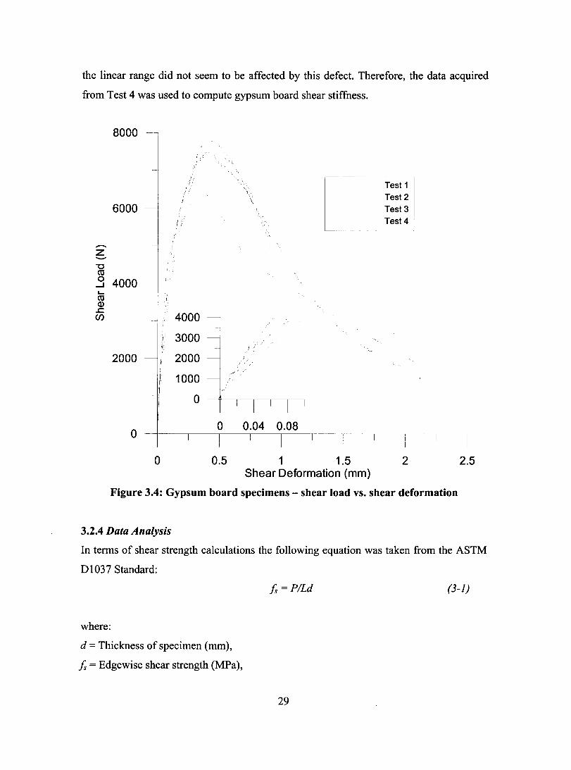
the linear range did not seem to be affected by this defect. Therefore, the data acquired
from Test 4 was used to compute gypsum board shear stiffness.
-Z -"0 ro
8000 -
6000
.3 4000 L-ro Q.) ~ Cf)
i ,
!
4000
3000
2000 2000
o
o
1000
o
.-.. '
o 0.04 0.08
0.5 1 1.5 Shear Deformation (mm)
Test 1 Test 2 Test 3 Test 4
2 2.5
Figure 3.4: Gypsum board specimens - shear load vs. shear deformation
3.2.4 Data Analysis
In terms of shear strength calculations the following equation was taken from the ASTM
D 1037 Standard:
where:
d = Thickness of specimen (mm),
!s = Edgewise shear strength (MPa),
!s =PILd (3-1)
29

L = Length of specimen (mm),
P = Maximum compressive load (N).
However, there is no recommended equation given in the ASTM standard to ca1culate the
stiffuess of the specimen for this specifie test setup. Two equations were used and the
results from both equations are shown. The two equations are presented below. The first
one is taken from the ASTM DI037, for shear stiffness (DI037a for this Thesis). This
equation was developed for a shear through the thickness of a plywood panel, therefore
the full width (b) of the specimen is used as opposed to the width between the rails.
G =P/dILbr (3-2)
where:
b = width of specimen (mm), taken as 88.9 mm (3.5"),
d = thickness of specimen (mm),
G = shear modulus (MPa),
L = length of specimen (mm),
P = load at proportionallimit, taken as 40% uItimate (N),
r = displacement of LVDT (mm).
The second stiffness equation, shown below is also taken from the ASTM Dl 037
(D 1 03 7b for this Thesis). This equation was developed by Boudreault (2005).
G = Pxb xF * Lxtxr
Where:
vp = Edgewise shear strength (MPa);
P max = Maximum compressive load (N);
G = Shear modulus (modulus ofrigidity) (MPa);
P = Compressive load (N);
b = Width of portion of the specimen in shear (mm) (b = 25.4 mm in this case);
L = Length of specimen (mm);
30
(3-3)

t = Average thickness of shear area (mm);
r = In-line displacement at load P (mm);
F = Multiplication factor to compensate nonuniform stress distribution in smaH
specimens. F= 1.19 (ASTM D2719, 1994)
The above equations were used to compute the values of the shear strength and stiffness
for aH the specimens. The results for stiffness and strength of the fibreboard and gypsum
board panels are shown in Tables 3.1 and 3.2, respectively.
Table 3.1: Two-sided shear test - fibreboard results
Test 2 Test 3 Test 4 TestS Test 6 Thickness (mm) 24.2 24.0 24.5 23.8 24.0
%CoV 0.77% 2.49% 1.66% 1.97% 1.38% 's (MPa) 0.88 1.05 1.11 1.02 1.09
Avg. '. (MPa) 1.07* %CoVof 'a 8.73%
ASTM 01037a - G (MPa) 134.6 105.4 152.4 253.7 232.7 Avg. G (MPa) 175 %CoVofG 36.7%
ASTM 01037b - G (MPa) 45.8 35.8 51.8 86.3 79.1 Avg. G (MPa) 59.8 %CoVofG 36.7%
*Note: the average/. was deternllned wlthout the result of Test 2.
Table 3.2: Two-sided shear test - gypsum results Test 1 Test 2 Test 3 Test 4
Thickness (mm) 15.4 15.2 15.2 15.4 %CoV 1.29% 0.83% 0.86% 3.11%
'. (MPa) 1.89 1.94 2.02 1.64 Avg.'. (MPa) 1.95*
%CoVof 'a 3.07% ASTM 01037a - G (MPa) 1460 1000 1240 1440
Avg. G (MPa) 1290 %CoVofG 16.6%
ASTM 01037b - G (MPa 497 340 423 488 Avg. G (MPa) 437 %CoVofG 16.6%
*Note: the average/. was detennined without the result of Test 4.
3.2.5 Discussion
It was found that on average the shear strength of the gypsum was approximately twice
that of the fibreboard. The average ultimate strength of the gypsum board, for this data
31
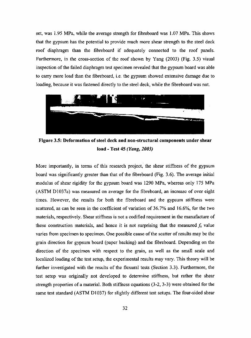
set, was 1.95 MPa, while the average strength for fibreboard was 1.07 MPa. This shows
that the gypsum has the potential to provide much more shear strength to the steel deck
roof diaphragm than the fibreboard if adequately connected to the roof panels.
Furthermore, in the cross-section of the roof shown by Yang (2003) (Fig. 3.5) visual
inspection of the failed diaphragm test specimen revealed that the gypsum board was able
to carry more load than the fibreboard, i.e. the gypsum showed extensive damage due to
loading, because it was fastened directly to the steel deck, while the fibre board was not.
Figure 3.5: Deformation of steel deck and non-structural components under shear
load - Test 45 (Yang, 2003)
More importantly, in terms of this research project, the shear stiffness of the gypsum
board was significantly greater than that of the fibreboard (Fig. 3.6). The average initial
modulus of shear rigidity for the gypsum board was 1290 MPa, whereas only 175 MPa
(ASTM D1037a) was measured on average for the fibreboard, an increase of over eight
times. However, the results for both the fibreboard and the gypsum stiffness were
scattered, as can be seen in the coefficient of variation of 36.7% and 16.6%, for the two
materials, respectively. Shear stiffness is not a codified requirement in the manufacture of
these construction materials, and hence it is not surprising that the measured!s value
varies from specimen to specimen. One possible cause of the scatter of results may be the
grain direction for gypsum board (paper backing) and the fibreboard. Depending on the
direction of the specimen with respect to the grain, as weIl as the small scale and
localized loading of the test setup, the experimental results may vary. This the ory will be
further investigated with the results of the flexural tests (Section 3.3). Furthermore, the
test setup was originally not developed to determine stiffness, but rather the shear
strength properties of a material. Both stiffness equations (3-2, 3-3) were obtained for the
same test standard (ASTM DI037) for slightly different test setups. The four-sided shear
32

test setup results (Section 3.4) willlater be relied on to provide additional information on
the shear stiffness of the non-structural components.
The two equations give very different results for local shear rigidity although they are
both taken from the ASTM DI037 standard. The interlaminar shear equation (DI037a)
gives a rigidity almost three times higher than the shear though the thickness equation
(DI037b). The results of the four-sided shear tests can be used to confirm which ofthese
two equations, if any, is adequate to calculate shear rigidity.
For comparison purposes the load vs. deformation curves for both the gypsum and
fibreboard are plotted in Figure 3.6. When comparing the gypsum board and the
fibreboard specimens, it is clear that the gypsum board has much higher local shear
rigidity than the fibreboard.
8000
6000
-z -'0 lU 0 4000 ....1 .... lU ID ..c en
2000
o 1
--- Fibreboard
Gypsum
2 3 4 Shear Deformation (mm)
5
Figure 3.6: Comparison of gypsum board and fibreboard specimens - shear load vs.
shear deformation
33

3.3 Flexural Test
3.3.1 Setup and Test Procedure
The flexural tests were conducted in order to obtain the flexural rigidity and strength of
the fibreboard and gypsum board panels. Even though the roof diaphragm structure is
assumed to be subjected to in-plane shear forces during lateral loading, due to the
warping deformation of the steel roof deck panels (Fig. 3.5), the flexural strength and
stiffness of the non-structural roofing components are of relevance (Yang, 2003). The
flexural test setup is a simple centre-point flexure test, which is based on ASTM Standard
C473 (1997). The loading plate and all bearing supports, which are rounded to a radius of
3.2 mm (Ys"), are the full width of the specimen. Figure 3.7 shows the test setup during
loading of a gypsum board specimen. The two bearing supports were placed at a distance
of355.6 mm (14").
The machine used for this setup was an MTS Sintech 30/G with a 150 kN load cell. Each
test was conducted in displacement control at a crosshead speed of 6.35 mm/sec (0.25
in/sec) until failure of the specimen. The load and the displacement of the crosshead
were used in the calculation of flexural properties.
l 'llllllii 1 - - --- -- ---- - ~ .'",::1" 1".-
Figure 3.7: Flexural test setup
3.3.2 Test Specimens
AlI test specimens were cut with a table and radial saw to 406.4 millimetres (16") long by
101.6 millimetres (4") wide, as per ASTM C473. The specimen dimensions were then
34

measured precisely using a micrometer and callipers. Three measurements were taken for
the width of each specimen and six were taken for the thickness. The arithmetic average
of the thickness and width for each specimen were used to compute the flexural stiffness
and strength. As required for the two-sided shear tests, test specimens were cut at least
four inches from the panel edges: aIl fibreboard specimens met this requirement.
However, specimens G-PLI, G-PLll, G-PL13, G-PL22, G-PPI, G-PP2, G-PPI2 and G
pp 13 were cut at less than 4 inches from the sides.
In aIl, 24 fibreboard specimens were tested. This included specimens FI to F16, which
were cut from a single panel but without a specific orientation with respect to the grain.
Eight additional specimens were cut from the same panel: Four were cut in one direction
and the other four were cut perpendicular to the previous specimens. These specimens
were labelled FDA and FDB, FDA meaning "Fibreboard Direction A" and FDB meaning
"Fibreboard Direction B." This approach was used to investigate the hypothesis that any
existing directionality of the wood fibres would affect the flexural properties. Directions
A and B have no precise meaning other than they are perpendicular to one another.
A total of 44 flexural gypsum board tests, consisting of two series of specimens, were
performed. The first series consisted of specimens parallei to the long side of the panel
(PL), while the second series was oriented perpendicular to the long side (PP). In the
identification of each test flexural specimen, the PL or PP designation is preceded by G,
identifying them as gypsum board specimens.
Gypsum board is typically fabricated with a finishing layer of paper on one side of the
panel. The fabrication direction of gypsum board panels is parallei to the long side of the
board. It was felt that this fabrication method may have an effect on the flexural stiffness
and strength of the panel depending on whether the paper was placed in tension or
compression during testing. Specimens G-PLI and G-PPI through G-PLII and G-PPII
were tested with the white finishing paper in compression. Specimens G-PL12 and G
PP12 through G-PL22 and G-PP22 were tested with the finishing paper in tension. These
specimens were cut from the same panel as the first specimens.
35

3.3.3 Specimen Behaviour
3.3.3.1 Fibreboard
Specimens FI through FI6 aIl behaved, in terms of flexural strength vs. stiffuess, in a
similar fashion. First, there existed a linear elastic range, which was then followed by a
decrease in stiffness (Fig. 3.8). The test specimen then reached its maximum load,
followed by a sudden brittle failure of the tensile fibres.
-z '-'
"C cu o
....J
250
200
150
100
50
o
o
-r--i-4 8 12 16
Displacement (mm)
Figure 3.8: Flexural test results - FI to F16
However, specimens FDA and FDB, which were cut perpendicular to one other, provided
test results which indicated that the behaviour of the fibreboard is direction dependent.
Figure 3.9 shows the load versus displacement curves for specimens FDA and FDB.
36
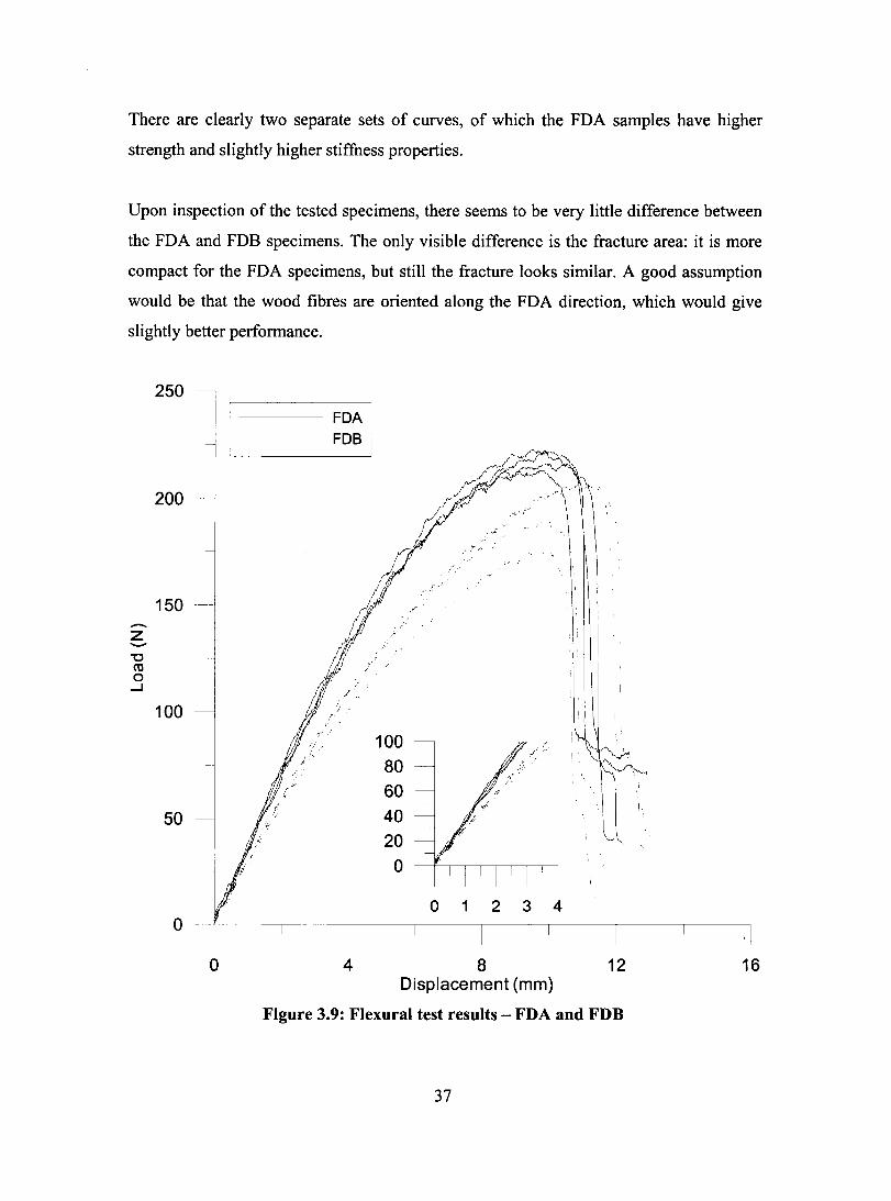
There are clearly two separate sets of curves, of which the FDA samples have higher
strength and slightly higher stiffness properties.
Upon inspection of the tested specimens, there seems to be very little difference between
the FDA and FDB specimens. The only visible difference is the fracture area: it is more
compact for the FDA specimens, but still the fracture looks similar. A good assumption
would be that the wood fibres are oriented along the FDA direction, which would give
slightly better performance.
-Z -"0 ca o ~
250
200
150
100
50
o
o
FDA 1
FDB
;' :
/ "
; 'j ,H
4 8 Displacement (mm)
12
Figure 3.9: Flexural test results - FDA and FDB
37
16

3.3.3.2 Gypsum Board
The gypsum board behaved quite differently from tibreboard for the flexural test. Figure
3.10 shows the behaviour of gypsum board with pp specimens where the tinishing paper
was in compression. There clearly exist two sections to the curve: tirst a linear elastic
range that extends to approximately 80-100 kN; second a yield plateau is developed until
a tinal brittle fracture of the specimen. Failure occurred on the tension side of the
specimen. The paper fails tirst, but at a low enough load that the gypsum itself still has
enough strength to resist the load applied. Cracks slowly propagate through the thickness
of the gypsum until the complete cross-section fractures.
-z -"0 cu o
...J
100
80
60
40
20
o
o 2 4 6 8 10 Displacement (mm)
Figure 3.10: Flexural test results - G-PPI to G-PPll
38

Specimens G-PPI2 through G-PP22, for which the finishing paper is in tension, behave
in roughly the same manner as specimens 1 through II. The capacity of the specimen is
slightly higher, probably due to the higher eapacity of the paper. When the paper breaks,
it goes down to roughly the same eapaeity as the previous specimens, which shows that
the gypsum itself seems isotropie (Fig. 3.11). The non-isotropie is probably due to paper
fibre orientation.
-Z ---0 ro o -1
120
80
40
o
o 246 8 10 Displacement (mm)
Figure 3.11: Flexural Test Results - G-PP12 to G-PP22
Figure 3.12 shows the behaviour of gypsum board with PL specimens. The behaviour is
mueh different from that of the pp specimens. The load versus displacement curve is
bilinear: at first a steep linear elastic curve up to approximately 150 N exists, which is
followed by a less steep linear zone that reaches approximately 300 N. This is followed
by a very brittle failure at a erosshead displacement between 8 and 10 millimetres. The
39
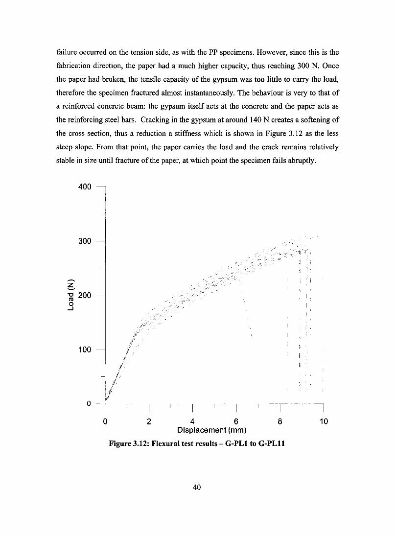
failure occurred on the tension side, as with the pp specimens. However, since this is the
fabrication direction, the paper had a much higher capacity, thus reaching 300 N. Once
the paper had broken, the tensile capacity of the gypsum was too little to carry the load,
therefore the specimen fractured almost instantaneously. The behaviour is very to that of
a reinforced concrete beam: the gypsum itself acts at the concrete and the paper acts as
the reinforcing steel bars. Cracking in the gypsum at around 140 N creates a softening of
the cross section, thus a reduction a stiffness which is shown in Figure 3.12 as the less
steep slope. From that point, the paper cames the load and the crack remains relatively
stable in size until fracture of the paper, at which point the specimen fails abruptly.
400
300
-z -'C 200 co o
....J
100
o
o
-'.'
2 4 6 Displacement (mm)
:.' ':. ::~:...:;:- ~~"fll', ' .< ~-:.:. ,.;.
""-:< -;:
8
! .
Figure 3.12: Flexural test results - G-PLI to G-PLll
40
10

Specimens PL-12 through PL-22 behaved in the same manner, although their ultimate
capacity was slightly lower. Still similar to a reinforced concrete beam, there are two
sections to the slope: the uncracked stiffness and the cracked stiffuess. From that point
the paper takes the load until it breaks. At that point, the load drops abruptly to zero.
300
- 200 z '-'
100
o
o
r·
Il ,Ji . . ' r'
)/ /7
l,V /
246 8 Displacement (mm)
Figure 3.13: Flexural test results - G-PL12 to G-PL22
3.3.4 Data Analysis
10
The two desired properties were the flexural strength and rigidity of the fibreboard and
gypsum board. In order to determine the flexural rigidity, El, the following ASTM D3043
(1995) equation was used:
EI= (L3/48)*(P/~) (3-4)
where:
E = Young's modulus in flexure (MPa),
41
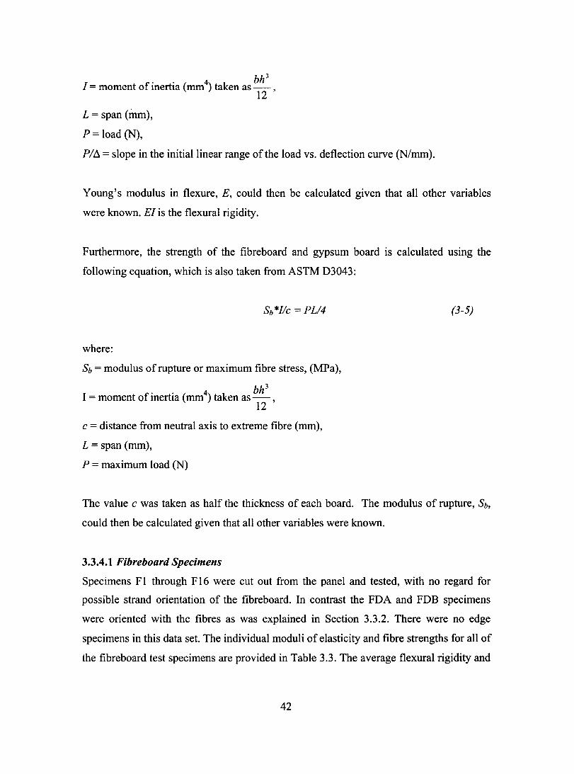
1 = moment of inertia (mm4) taken as bh3
,
12
L = span (mm),
P = load (N),
PIIl = slope in the initiallinear range of the load vs. deflection curve (N/mm).
Young's modulus in flexure, E, could then be calculated given that aIl other variables
were known. El is the flexural rigidity.
Furthermore, the strength of the fibre board and gypsum board is calculated using the
foIlowing equation, which is also taken from ASTM D3043:
Sb *l/c = PLI4
where:
Sb = modulus of rupture or maximum fibre stress, (MPa),
1 = moment ofinertia (mm4) taken as bh
3
, 12
c = distance from neutral axis to extreme fibre (mm),
L = span (mm),
P = maximum load (N)
(3-5)
The value c was taken as half the thickness of each board. The modulus of rupture, Sb,
could then be calculated given that aIl other variables were known.
3.3.4.1 Fibreboard Specimens
Specimens FI through F 16 were cut out from the panel and tested, with no regard for
possible strand orientation of the fibreboard. In contrast the FDA and FDB specimens
were oriented with the fibres as was explained in Section 3.3.2. There were no edge
specimens in this data set. The individual moduli of elasticity and fibre strengths for aIl of
the fibreboard test specimens are provided in Table 3.3. The average flexural rigidity and
42
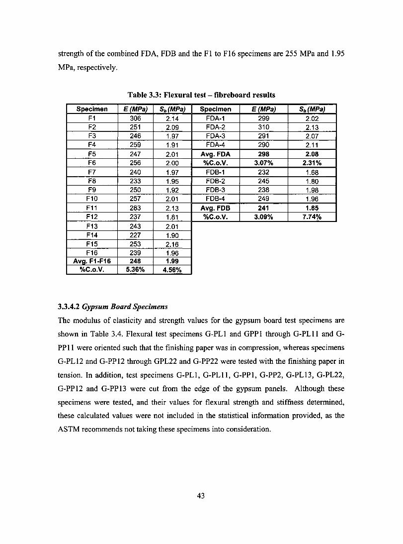
strength of the combined FDA, FDB and the FI to F16 specimens are 255 MPa and 1.95
MPa, respectively.
Table 3.3: Flexural test - tibreboard results
Specimen E(MPa) Sb (MPa) Specimen E(MPa) Sb (MPa) F1 306 2.14 FDA-1 299 2.02 F2 251 2.09 FDA-2 310 2.13 F3 246 1.97 FDA-3 291 2.07 F4 259 1.91 FDA-4 290 2.11 F5 247 2.01 Avg. FOA 298 2.08 F6 256 2.00 %C.o.V. 3.07% 2.31% F7 240 1.97 FDB-1 232 1.68 F8 233 1.95 FDB-2 245 1.80 F9 250 1.92 FDB-3 238 1.98
F10 257 2.01 FDB-4 249 1.96 F11 283 2.13 Avg. FOB 241 1.85 F12 237 1.81 %C.o.V. 3.09% 7.74%
F13 243 2.01 F14 227 1.90 F15 253 2.16 F16 239 1.96
Avg. F1-F16 248 1.99 %C.o.V. 5.36% 4.56%
3.3.4.2 Gypsum Board Specimens
The modulus of elasticity and strength values for the gypsum board test specimens are
shown in Table 3.4. Flexural test specimens G-PL1 and GPP1 through G-PLll and G
pp Il were oriented such that the finishing paper was in compression, whereas specimens
G-PL12 and G-PP12 through GPL22 and G-PP22 were tested with the finishing paper in
tension. In addition, test specimens G-PL1, G-PLll, G-PP1, G-PP2, G-PL13, G-PL22,
G-PP12 and G-PP13 were cut from the edge of the gypsum panels. Although these
specimens were tested, and their values for flexural strength and stiffness determined,
these calculated values were not inc1uded in the statistical information provided, as the
ASTM recommends not taking these specimens into consideration.
43
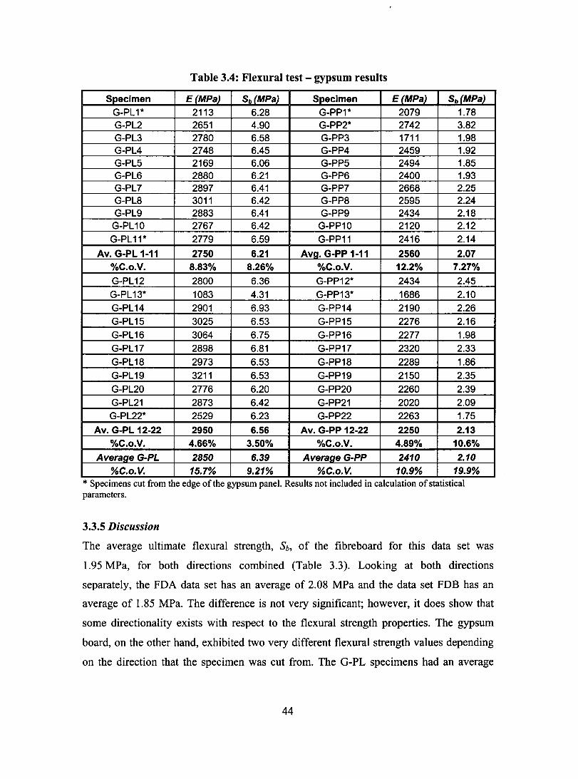
Table 3.4: Flexural test - gypsum results
Specimen E(MPa) Sb (MPa) Specimen E(MPa) Sb (MPa) G-PL 1* 2113 6.28 G-PP1* 2079 1.78 G-PL2 2651 4.90 G-PP2* 2742 3.82 G-PL3 2780 6.58 G-PP3 1711 1.98 G-PL4 2748 6.45 G-PP4 2459 1.92 G-PL5 2169 6.06 G-PP5 2494 1.85 G-PL6 2880 6.21 G-PP6 2400 1.93 G-PL7 2897 6.41 G-PP7 2668 2.25 G-PL8 3011 6.42 G-PP8 2595 2.24 G-PL9 2883 6.41 G-PP9 2434 2.18 G-PL 10 2767 6.42 G-PP10 2120 2.12
G-PL 11* 2779 6.59 G-PP11 2416 2.14
Av. G-PL 1-11 2750 6.21 Avg. G-PP 1-11 2560 2.07 %C.o.V. 8.83% 8.26% %C.o.V. 12.2% 7.27%
G-PL12 2800 6.36 G-PP12* 2434 2.45
G-PL 13* 1083 4.31 G-PP13* 1686 2.10 G-PL 14 2901 6.93 G-PP14 2190 2.26 G-PL15 3025 6.53 G-PP15 2276 2.16
G-PL16 3064 6.75 G-PP16 2277 1.98
G-PL17 2898 6.81 G-PP17 2320 2.33
G-PL18 2973 6.53 G-PP18 2289 1.86
G-PL19 3211 6.53 G-PP19 2150 2.35
G-PL20 2776 6.20 G-PP20 2260 2.39
G-PL21 2873 6.42 G-PP21 2020 2.09
G-PL22* 2529 6.23 G-PP22 2263 1.75
Av. G-PL 12-22 2950 6.56 Av. G-PP 12-22 2250 2.13 %C.o.V. 4.66% 3.50% %C.o.V. 4.89% 10.6%
Average G-PL 2850 6.39 Average G-PP 2410 2.10 %C.o.v. 15.7% 9.21% %C.o.V. 10.9% 19.9%
* SpecImens cut from the edge of the gypsum panel. Results not mcluded 10 calculatlOn of statIstICal parameters.
3.3.5 Discussion
The average ultimate flexural strength, Sb, of the fibreboard for this data set was
1.95 MPa, for both directions combined (Table 3.3). Looking at both directions
separately, the FDA data set has an average of 2.08 MPa and the data set FDB has an
average of 1.85 MPa. The difference is not very significant; however, it does show that
sorne directionality exists with respect to the flexural strength properties. The gypsum
board, on the other hand, exhibited two very different flexural strength values depending
on the direction that the specimen was cut from. The G-PL specimens had an average
44
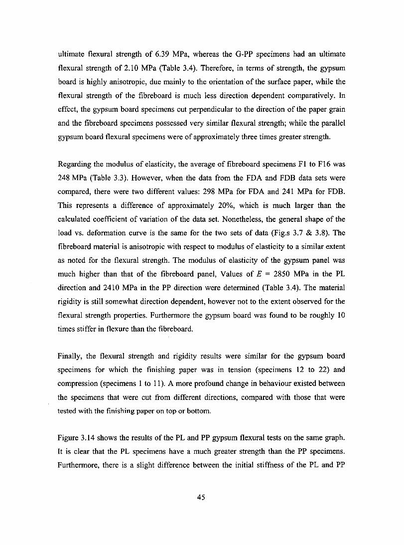
ultimate flexural strength of 6.39 MPa, whereas the G-PP specimens had an ultimate
flexural strength of 2.10 MPa (Table 3.4). Therefore, in terms of strength, the gypsum
board is highly anisotropic, due mainly to the orientation of the surface paper, while the
flexural strength of the fibreboard is much less direction dependent comparatively. In
effect, the gypsum board specimens cut perpendicular to the direction of the paper grain
and the fibreboard specimens possessed very similar flexural strength; while the parallel
gypsum board flexural specimens were of approximately three times greater strength.
Regarding the modulus of elasticity, the average of fibreboard specimens FI to F16 was
248 MPa (Table 3.3). However, when the data from the FDA and FDB data sets were
compared, there were two different values: 298 MPa for FDA and 241 MPa for FDB.
This represents a difference of approximately 20%, which is much larger than the
calculated coefficient of variation of the data set. Nonetheless, the general shape of the
load vs. deformation curve is the same for the two sets of data (Fig.s 3.7 & 3.8). The
fibre board material is anisotropic with respect to modulus of elasticity to a similar extent
as noted for the flexural strength. The modulus of elasticity of the gypsum panel was
much higher than that of the fibreboard panel, Values of E = 2850 MPa in the PL
direction and 2410 MPa in the PP direction were determined (Table 3.4). The material
rigidity is still somewhat direction dependent, however not to the extent observed for the
flexural strength properties. Furthermore the gypsum board was found to be roughly 10
times stiffer in flexure than the fibreboard.
Finally, the flexural strength and rigidity results were similar for the gypsum board
specimens for which the finishing paper was in tension (specimens 12 to 22) and
compression (specimens 1 to Il). A more profound change in behaviour existed between
the specimens that were cut from different directions, compared with those that were
tested with the finishing paper on top or bottom.
Figure 3.14 shows the results of the PL and PP gypsum flexural tests on the same graph.
It is clear that the PL specimens have a much greater strength than the PP specimens.
Furthermore, there is a slight difference between the initial stiffuess of the PL and PP
45
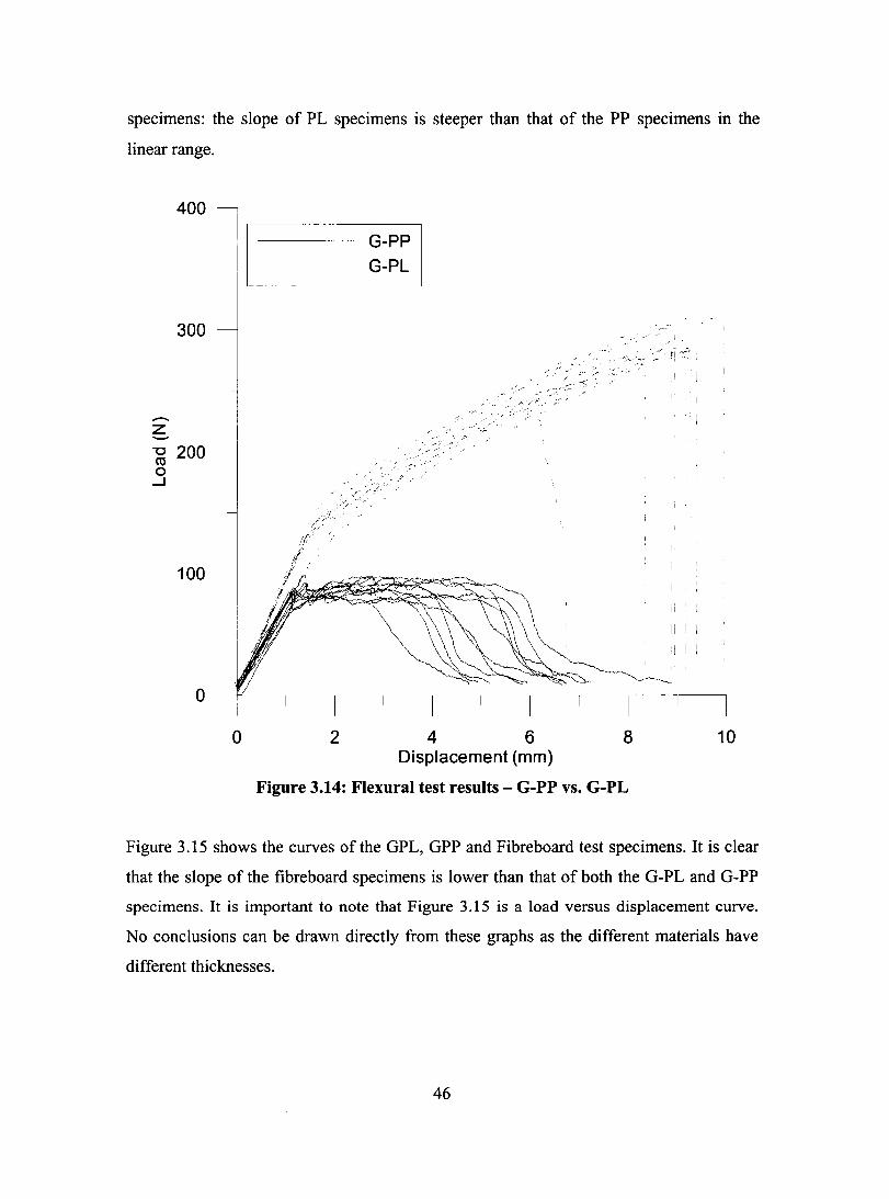
specimens: the slope of PL specimens is steeper than that of the PP specimens in the
linear range.
400
300
-Z -"0 200 m o
...J
100
o
o
G-PP
G-PL
<' - '--:> .... "'.:.-: -~',' -' .. , '.~... ',<.-: .;:", : "
,.r- -:<.' '
'. -.:-;;
-/" ,,'
. : -;;." ,>~;.J.:" .
1//" i
2 4 6 8 Displacement (mm)
Figure 3.14: Flexural test results - G-PP vs. G-PL
, ,
ii 1 J
,!
10
Figure 3.15 shows the curves of the GPL, GPP and Fibreboard test specimens. It is clear
that the slope of the fibreboard specimens is lower than that of both the G-PL and G-PP
specimens. It is important to note that Figure 3.15 is a load versus displacement curve.
No conclusions can be drawn directly from these graphs as the different materials have
different thicknesses.
46
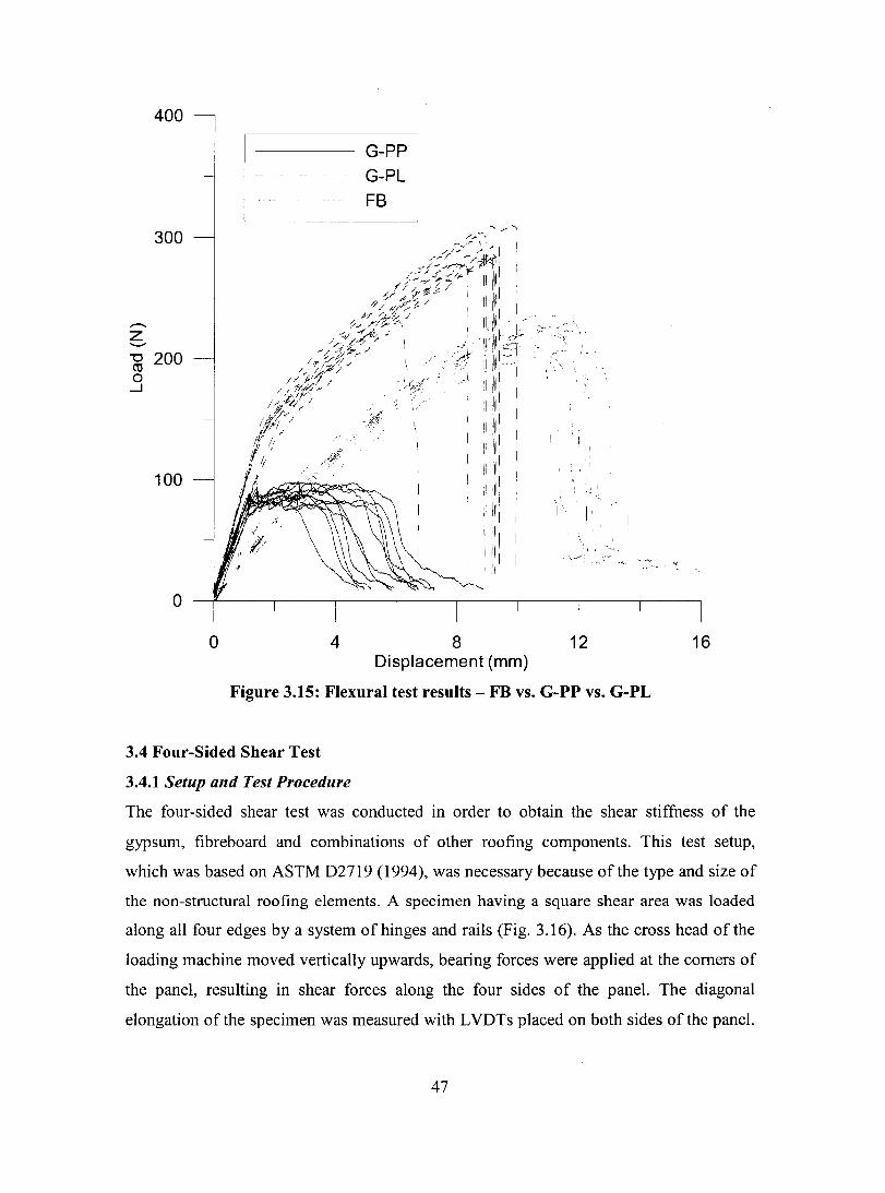
400
300
Z
"0 200 co o
..J
100
o
o
G-PP --- .- - --- -~ G-PL
FB
4 8 Displacement (mm)
12
Figure 3.15: Flexural test results - FB vs. G-PP vs. G-PL
3.4 Four-Sided Shear Test
3.4.1 Setup and Test Procedure
16
The four-sided shear test was conducted in order to obtain the shear stiffness of the
gypsum, tibreboard and combinations of other rooting components. This test setup,
which was based on ASTM D2719 (1994), was necessary because of the type and size of
the non-structural roofing elements. A specimen having a square shear area was loaded
along aIl four edges by a system ofhinges and rails (Fig. 3.16). As the cross head of the
loading machine moved vertically upwards, bearing forces were applied at the corners of
the panel, resulting in shear forces along the four sides of the panel. The diagonal
elongation of the specimen was measured with LVDTs placed on both sides of the panel.
47

With the acquired data, the shear load versus shear deformation curves were plotted, from
which the stiffuess of the material was calculated. The panels were not tested to failure
because the objective of these tests was to measure the shear stiffuess parameters and not
the ultimate strength.
o
Figure 3.16: Four-sided shear test frame
To avoid bearing at the ends of the panel and to provide a more uniform transfer ofshear,
two 19 mm (3/4") thick plywood rails were screw fastened to the panel along each edge.
Figure 3.17 shows a c1ose-up of the hinge area, with the plywood rails fastened to a
gypsum board test specimen. Thus the bearing load was applied to the ends of the
plywood rails, not directly to the panel. The rails, which were secured with 10 to 12
drywall screws, then transferred the applied loads in a uniform fashion to the test
specimen. To secure the rails to the gypsum board, 6xl" gypsum screws were used
whereas the fibreboard required 6x2" screws because of the higher thickness.
48

Figure 3.17: Dinge are a close-up
The most important aspect of the test setup was the alignment of the test specimen. It was
necessary to ensure that the specimen was directly in line with the centre of the load cell
and bottom support. The impact of any eccentricity in the installation of the test specimen
is further discussed in Section 3.4.3.
The machine used for this setup was an MTS Sintech 30/G with a 150 kN load cell. Each
test was conducted in displacement control at a crosshead speed of 2.1 mm/min (0.083
in/min). The L VDTs and load cell were connected to a Vishay Model 5100B scanner,
which was used to record the data using the Vishay System 5000 StrainSmart software.
The loading rate was determined using the recommendations of ASTM D2719, as
follows:
n = ZL/J2 (3-6)
where:
n = speed of crosshead (mm/min),
L = length of side of shear area (mm),
49
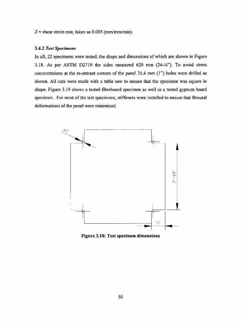
Z = shear strain rate, taken as 0.005 (mm/mm/min).
3.4.2 Test Specimens
In all, 22 specimens were tested, the shape and dimensions of which are shown in Figure
3.18. As per ASTM D2719 the sides measured 620 mm (24-W'). To avoid stress
concentrations at the re-entrant corners of the panel 25.4 mm (1") holes were drilled as
shown. AlI cuts were made with a table saw to ensure that the specimen was square in
shape. Figure 3.19 shows a tested tibreboard specimen as well as a tested gypsum board
specimen. For most of the test specimens, stiffeners were installed to ensure that flexural
deformations of the panel were minimized.
o]//
b
.'.ru 0
1 ,
ru
1
5" - -Figure 3.18: Test specimen dimensions
50

Figure 3.19: Fibreboard specimen (Ieft); Gypsum specimen (right)
Figure 3.20: Fibreboard specimen (Ieft); Hot bitumen application (right)
Of the 22 specimens, eight tibreboard panels and seven gypsum panels were tested in the
setup described above. These specimens are referred to by the name FB for tibreboard
and FB-STIFF for tibreboard with a stiffener, as well as GYP-STIFF for gypsum with a
stiffener. In addition to these single panel specimens, it was necessary to fabricate
specimens that consisted of combinations of tibreboard, ISO insulation, felt vapour
retarder and gypsum. These test specimens were similar to the diaphragm specimens with
non-structural components tested by Yang (2003). For three tests a 25.4 mm (1") by
609mm by 609mm (24"x24") insulation board was hot bitumen adhered to a tibreboard
51

panel, as shown in Figure 3.20. These specimens were called FB+ISO. Figure 3.21
shows the fini shed product once the insulation board had been added on top of the
fibreboard.
Figure 3.21: FB+ISO specimen plan view (left); FB+ISO specimen cross-section view (right)
A total of four FULL SECTION specimens were fabricated in an attempt to represent the
non-structural components of a roof. A 609mm by 609mm (24"x24") sheet of felt vapour
retarder was first hot bitumen adhered to the FB+ISO section. As a second step in the
fabrication a 609mm by 609mm (24"x24") gypsum layer was then hot bitumen adhered
to the vapour retarder. Figure 3.22 shows a plan view and an elevation view of a fini shed
speclmen.
52

Figure 3.22: FULL SECTION specimen plan view (Ieft); FULL SECTION specimen cross-section view (right)
The fibreboard was used as the base material in aIl the "sandwich" constructions
specimens because it has a lower stiffness than the gypsum board. This facilitated the
measurement of any change in stiffness as the additional non-structural layers were
added. If gypsum had been used as the base material, the relative increase in stiffness
due to the added layers would have been much lower than the stiffness of the gypsum
itself, perhaps even negligible. Also, note that only the fibreboard was sandwiched
between the two plywood rails; the other non-structural layers were located within the
central portion of the test specimen, as can be seen in Figure 3.18. These specimens were
tested in the same test setup as the plain gypsum board and fibreboard specimens (Fig.
3.23).
53

Figure 3.23: FULL SECTION specimen in test frame before loading
The ISO insulation board could not be tested by itself because of its relative shear
flexibility and its thickness. The testing frame as fabricated could not accommodate for
this thickness and type of material.
The thickness and length were precisely measured for each specimen before it was tested.
For the FB+ISO and the FULL SECTION specimens, only the thickness and length of
the fibre board base was taken into account. The reasons behind this will be further
explained in Section 3.4.4.
3.4.3 Specimen Behaviour
3.4.3.1 Unstiffened Specimens
In aH, four unstiffened fibreboard panels and one unstiffened gypsum panel were tested.
Although the ASTM D2719 test setup was respected, the failure mechanism was not what
was expected: a shear buckling failure of the panel in the vertical plane due to horizontal
54

compression forces occurred rather than a shear failure. Figure 3.24 shows the load paths
that exist in this type of test specimen. Because of this failure mode the results from these
specimens were not considered to represent the in-plane shear stiffuess of the fibreboard
and gypsum panels, and hence were not used.
..
Figure 3.24: Panelload forces
3.4.3.1.1 Addition of Stiffeners
Flexural deformations were quite significant in the first test specimens. Stiffening the
panels was attempted by testing two panels at once. The two panels were screwed
together with 6x2" gypsum screws. This procedure did reduce the amount of buckling
that occurred in the specimen, but not completely: failure still occurred by buckling. In
light of these results, a second method was conceived.
To counter the problem of buckling, a horizontal stiffener angle (50mm x 50mm x
6.5mm) was attached to each side of the test panel to increase its flexural rigidity and
strength (Fig. 3.25). The angles were attached at three locations with 12.7 mm (112")
threaded rods. The centre threaded rod hole was circular, while the two end holes were
55

slotted to allow for any axial defonnations of the panel and to ensure that the angles did
not carry any axial force. The nuts on the end threaded rods were hand-tightened to
minimize any friction forces between the panel and the angles. This stiffener setup was
used for aIl of the remaining tests.
-
.-- -
h
- ~
-
Figure 3.25: Stiffener installed on gypsum board panel
3.4.3.2 FB-STIFF (Stiffened Fihrehoard).
A typical load versus elongation curve for a fibreboard shear specimen is provided in
Figure 3.26. The two plots provide the readings for the two L VDTs that were installed on
each specimen. The load versus elongation curves for fibre board panels were very
consistent in shape. The first part of the graph, where the two curves are moving in
different directions represents the straightening of the panel. There typically exists a
56
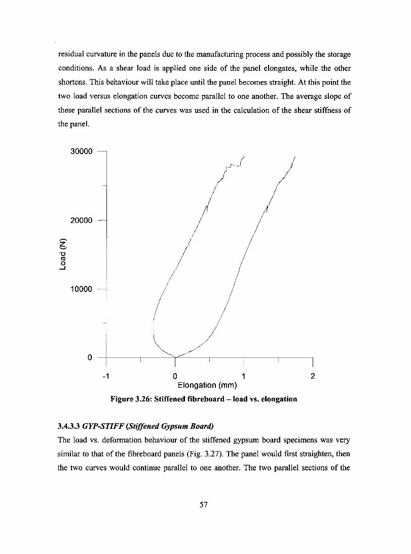
residual curvature in the panels due to the manufacturing process and possibly the storage
conditions. As a shear load is applied one side of the panel elongates, while the other
shortens. This behaviour will take place until the panel becomes straight. At this point the
two load versus elongation curves become parallel to one another. The average sI ope of
these parallel sections of the curves was used in the calculation of the shear stiffuess of
the panel.
30000
20000
...-.. Z -"0 co 0
.....J
10000
o
-1 o 1 2 Elongation (mm)
Figure 3.26: Stiffened tibreboard - Joad vs. eJongation
3.4.3.3 GYP-STIFF (Stiffened Gypsum Board)
The load vs. deformation behaviour of the stiffened gypsum board specimens was very
similar to that of the fibreboard panels (Fig. 3.27). The panel would first straighten, then
the two curves would continue parallel to one another. The two parallel sections of the
57

curves were once again used to detennine the shear stiffness of the test panel. The results
for the gypsum board tests were also consistent in shape.
25000
20000
15000 ......... Z -"0 co 0
.....J
10000
5000
o 1 ----
T 1 -1 o 1 2
Elongation (mm)
Figure 3.27: Stiffened gypsum board -load vs. elongation
3.4.3.4 ~ll-rI~l)
The load versus displacement curve of the FB-rISO specimens, shown in Figure 3.28,
were similar in shape to the curves obtained for the fibreboard panels alone. However,
upon doser inspection it can be seen that the two curves, once the specimen had
straightened, did not ron parallel to one another. For these tests an LVDT was attached
58
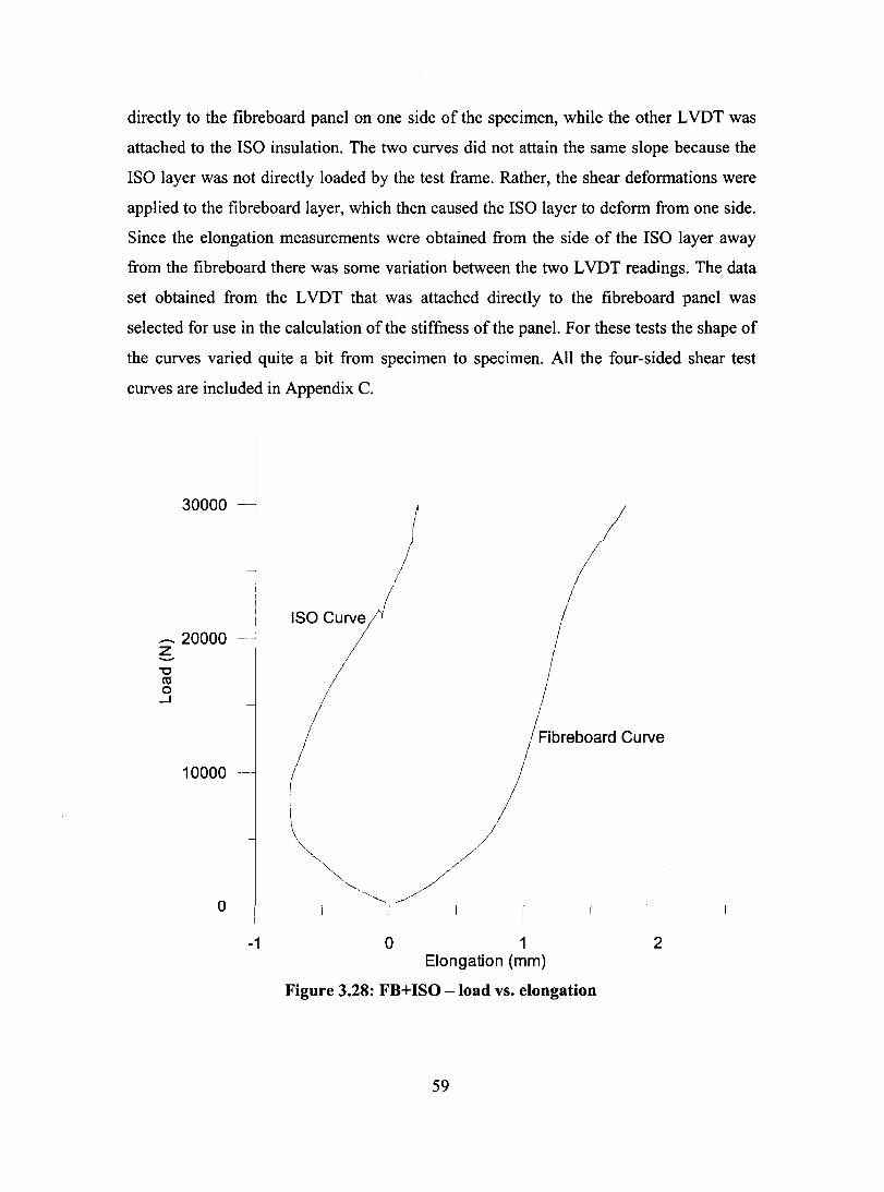
directly to the fibre board panel on one side of the specimen, while the other L VDT was
attached to the ISO insulation. The two curves did not attain the same slope because the
ISO layer was not directly loaded by the test frame. Rather, the shear deformations were
applied to the fibreboard layer, which then caused the ISO layer to deform from one side.
Since the elongation measurements were obtained from the side of the ISO layer away
from the fibreboard there was sorne variation between the two L VDT readings. The data
set obtained from the L VDT that was attached directly to the fibreboard panel was
selected for use in the calculation of the stiffuess of the panel. For these tests the shape of
the curves varied quite a bit from specimen to specimen. AB the four-sided shear test
curves are included in Appendix C.
30000
.- 20000 ~ ~ CIl o ~
10000
o
-1
ISO Curve
o
Fibreboard Curve
1 Elongation (mm)
2
Figure 3.28: FB+ISO - load vs. elongation
59
--1
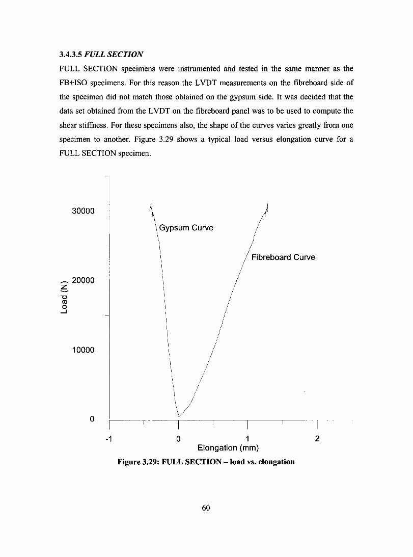
3.4.3.5 FULL SECTION
FULL SECTION specimens were instrumented and tested in the same manner as the
FB+ISO specimens. For this reason the LVDT measurements on the tibreboard side of
the specimen did not match those obtained on the gypsum side. It was decided that the
data set obtained from the L VDT on the tibreboard panel was to be used to compute the
shear stiffness. For these specimens also, the shape of the curves varies greatly from one
specimen to another. Figure 3.29 shows a typical load versus elongation CUrve for a
FULL SECTION specimen.
30000
_ 20000 z -"0 cu o
...J
10000
o
-1
Gypsum Curve
o
Fibreboard Curve
1 Elongation (mm)
Figure 3.29: FULL SECTION -load vs. elongation
60
2
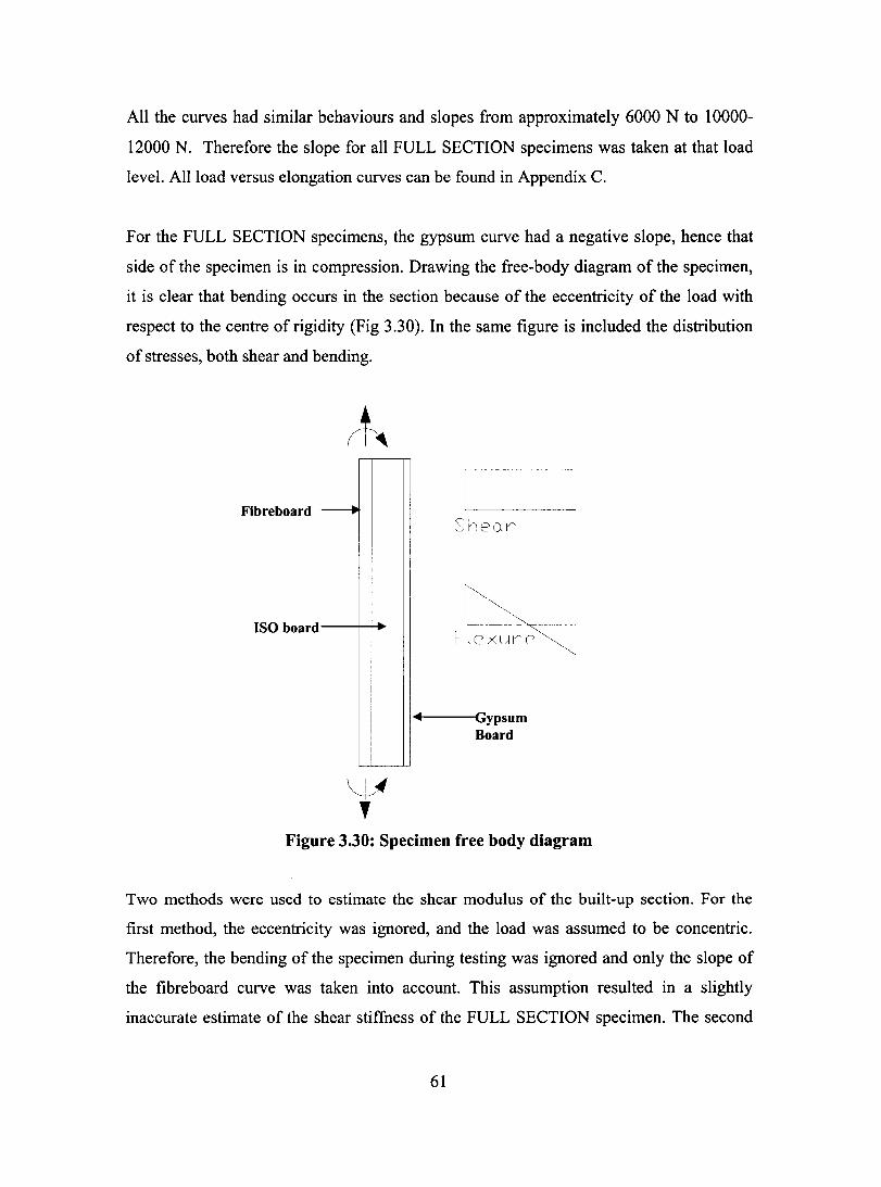
AU the curves had similar behaviours and slopes from approximately 6000 N to 10000-
12000 N. Therefore the slope for aU FULL SECTION specimens was taken at that load
level. Allload versus elongation curves can be found in Appendix C.
For the FULL SECTION specimens, the gypsum curve had a negative slope, hence that
side of the specimen is in compression. Drawing the free-body diagram of the specimen,
it is clear that bending occurs in the section because of the eccentricity of the load with
respect to the centre of rigidity (Fig 3.30). In the same figure is included the distribution
of stresses, both shear and bending.
Fibreboard -----
ISO board
...
1
Sh eo.r
l' Fl exure
Gypsum Board
Figure 3.30: Specimen free body diagram
Two methods were used to estimate the shear modulus of the built-up section. For the
first method, the eccentricity was ignored, and the load was assumed to be concentric.
Therefore, the bending of the specimen during testing was ignored and only the slope of
the fibre board curve was taken into account. This assumption resulted in a slightly
inaccurate estimate of the shear stiffness of the FULL SECTION specimen. The second
61

method consisted of building a finite element model of the built-up section and obtaining
the shear modulus of the FULL SECTION specimen from the analyses. Both methods
will be further discussed in Section 3.4.5. This investigation was needed to interpret the
results of the FB-ISO and FULL SECTION tests due to eccentricity present in the
speCImens.
3.4.4 Data Analysis
3.4.4.1 Concentrically loaded specimen
The stiffness of each test panel was obtained from the load vs. elongation graphs
described previously and Equation 3.6 from ASTM D2073 (1994). This equation has
been formulated for use with the four-sided shear test.
G = 0.3536(Plt::..)*[L, / (L*t)]
where:
G = modulus ofrigidity (MPa),
PIt::.. = slope offorce/deformation curve (N/mm)
LI = gauge length (mm),
L = length of side of shear areas (mm),
t = thickness of shear specimen (mm).
It is possible to derive this equation from the fOllowing:
G=rl"(
where:
r = shear stress defined as PI (2sin 45) * 2sin 451 (L * t) = PI (L * t), -y= shear strain defined as (2&os 45) / (L, 12cos45) = t::..1 (0.3536 * LÛ.
(3-6)
(3-7)
The thickness of the shear specimen, t, was defined simply as the thickness of the
fibreboard or gypsum panels when either of these two materials were tested alone.
However, for the FB+ISO and FULL SECTION specimens, the thickness was taken as
62
that of the tibreboard panel. With this assumption, it was possible to determine the
contribution provided by the insulation board and the gypsum board in terms of an
increased stiffness for the tibreboard. That is, the other non-structural layers were simply
thought of as reinforcement for the tibreboard test specimen. As noted previously, the
average slope of the two deformation curves once the test panel had straightened was
taken as P/,tj for the gypsum and tibreboard specimens. In the case of the FB+ISO and
FULL SECTION specimens, only the data acquired from the L VDT on the tibreboard
panel was used to calculate the slope of the load vs. elongation graph. The results of the
four-sided shear test have been provided in Table 3.5.
The test values for the unstiffened specimens are shown only for comparison with the
stiffened specimens. FB 1, FB2 and FB3 provided adequate results; it seems that buckling
was not problematic for the tibreboard specimens. However it is clear that for the
unstiffened gypsum specimen, buckling resulted in a severe reduction in stiffuess (see
Table 3.5). GYP-STIFFI was installed incorrectly in the test frame which explains the
very low stiffness value that was obtained even though the stiffener had been attached.
63

0'1 .J:>.
Table 3.5: Four-sided shear test results
Specimen FB1 FB2 FB3 FB4+FB5
G (MPa) 234 241 263 388
Average 282
%C.o.V. 25.6%
Specimen FB2-STIFF FB3-STIFF FB4-STIFF FB5-STIFF
G (Mpa) 287 198 265 191
Average 235
%C.o.V. 20.4%
Specimen GYP1-STIFF GYP2-STIFF GYP3-STIFF GYPS4-STIFF
G(MPa) 281* 1423 229* 997
Average 1284
%C.o.V. 15.11%
Specimen FB+IS01 FB+IS02 FB+IS03
G(MPa) 265 352 302
Average 306
%C.o.V. 14.13%
Specimen FULL SECTION1 FULL SECTION2 FULL SECTION3 FULL SECTION4
G(MPa) 401 280 310 492
Average 395
%C.o.V. 18.89%
* Specimens were not used to calculate average values.
GYP1
259
NIA
NIA
GYP5-STIFF GYP6-STIFF
1355 1363

3.4.5 Discussion
Upon reviewing the various results obtained from the four-sided shear tests, it became
c1ear that the gypsum board had the highest in-plane shear stiffness of aIl the materials
tested. Its average shear stiffness of 1284 MPa was 5.5 times higher than that of the
tibreboard (235 MPa) (Table 3.5). However, the most interesting information obtained
from this experimental research is the data from the FB+ISO and FULL SECTION
specimens. Firstly, the results using the concentric load method will be discussed,
followed by the results of a tinite element analysis.
3.4.5.1 Concentric Load Analysis
An increase in shear stiffness of 30 %, compared with the tibreboard alone, was
measured (Table 3.5) when the ISO board was added to the tibreboard. A total shear
stiffness increase of almost 70% compared to the tibreboard al one and an increase of
almost 30% compared to FB+ISO were realised when the gypsum board and vapour
retarder layers were added to the tibreboard and ISO board. However, it must be noted
that these values may not be accurate because the concentric data analysis did not take
into account the eccentric loading of the test specimen.
These results provide the stiffness of the rooting section with the load applied to the
tibreboard. However, in the actual roof section, as shown in Figure 3.31, the shear load /
deformation would tirst be applied to the gypsum board from the corrugated steel roof
deck panels. Screw fasteners are typically used to connect the gypsum board to the deck
panels. Hence, what needs to be addressed is the increase in stiffness to the gypsum board
because of the addition of the vapour retarder, ISO and tibreboard panels.
65

.~.
Figure 3.31: Roof Cross-Section (Yang, 2003)
The stiffness of the fibreboard and gypsum board panels is known, as well as the FULL
SECTION and the FB+ISO section. The only individual non-structural component for
which the shear stiffness is not known is the ISO board, excluding the vapour retarder
which can be assumed to have negligible in-plane shear stiffness. For this reason an
attempt was made to determine the stiffness of the ISO board given the test results listed
in Table 3.5. Figure 3.32 shows the spring model that was used to represent the non
structural roofing cross section. The gypsum board was connected in parallel because it is
directly attached to the steel deck, whereas the fibreboard and ISO board are attached in
series. This approach was taken because the fibreboard and ISO layers, although they
may stiffen the diaphragm, are not mechanically fastened to the steel deck.
66

Kgyp
Figure 3.32: Spring-stiffness diagram of non-structural roofing components
This same correlation can be used for the FULL SECTION four-sided test specimens.
Using the same concept and inversing the position of Kjb and Kgyp, it was possible to
compute the value of K iso . The modified spring diagram used to compute the ISO board
stiffness is shown in Figure 3.33.
Kgyp
Figure 3.33: Modified spring-stiffness dia gram of nonstructural roofing components
Simply by using Ohm's law, Equation 3-7 can be derived as:
K full = K fb + (_1_ + _l_J-1 , Kgyp K iso
Isolating K iso :
67
(3-7)
Kiso
-1 = (K full - K lb )-1 __ 1_ Kgyp
(3-8)
Using the average values listed in Table 3.5 and Equation 3-8, K jso is calculated to be
184 MPa. With this value, the stiffness of the full section, Ksys, with the gypsum board as
the base element can be computed. Using this approach the in,..plane shear stiffness of the
non-structural roofing components was found to be 1387 MPa.
3.4.5.2 Finite Element Analysis
In order to obtain a more realistic evaluation of the shear modulus of the built-up section,
two linear elastic finite element models (FEM) were developed using the SAP2000
software. Firstly, a finite element model resembling the four-sided shear test specimen
was built (Fig. 3.34). Loads were applied along the edges of the fibreboard panel in order
to simulate the shear load applied by the test frame. As Figure 3.34 shows, bending
occured in the built-up section due mainly to the eccentric loading. However, the values
of E and G of the ISO board were unknown; therefore this mode! was used to obtain the
value of the shear modulus and the modulus of el asti city of the polyisocyanurate panel.
The deformation of the model was obtained at the same locations as were used to
measure the deformation of the test specimens, followed by a comparison of the analysis
results with the test results. A constant Poisson's ration, chosen as 0.3, was maintained
throughout the parametric study. The values of E and G were systematically varied until
the analytical deformations matched those measured during testing.
The models shown in Figures 3.34 and 3.35 were built using eight-node Salid Elements.
These elements are direct extensions of rectangular plane element or shell elements
(Cook et al., 2001) and are produced by using the Extrude function. It is possible for
strains and stresses to vary through the thickness of these elements. The model shown in
Figure 3.34 has 1728 solid elements, 576 for each material. Continuity between the
different solid elements is automatically recreated if adjacent solid elements are built
using the same joints. If two faces of two distinct solid elements are bound by the same
joints, the deformations of the two faces will be same for the whole surface of that face
because their displacements are controlled by the same polynomial displacement field.
68

The elements are assigned the material properties of gypsum board and fibreboard that
were obtained in Sections 3.3 and 3.4.
Figure 3.34: Undeformed (Ieft) and deformed (right) FEM of FULL SECTION test
specimen
It is mentioned in the literature that values for the shear modulus of elasticity of
polyisocyanurate foams used in sandwich construction vary from 0 to 5 MPa (Vinson,
1999). Rence, the initial value of E, combined with a Poisson's ratio of 0.3, was assumed
to be in this range. Upon successful correlation of the analysis and test results, the
modulus of elasticity and the shear modulus of the polyisocyanurate board were
determined to be 9.4 MPa and 4.0 MPa, respectively.
Once the material properties of the three non-structural components had been obtained, a
second FEM was built (Fig. 3.35). A simple cantilever analysis model composed of only
the gypsum, ISO and fibreboard layers was constructed. The model is 24" by 24", the
same dimensions as the test specimen without the loading rails. The same eight-node
element types were used in the model, although only three elements were required, one
for each layer of material (Figure 3.35). The four sided shear test model was divided into
thousands of elements primarily because it was necessary to obtain displacement readings
at the specific locations that were used in the testing procedures. Furthermore, more
accurate results for flexure will be obtained by using multiple elements, whereas shear
deformation accuracy is not affected by the number of elements (Cook et al., 2001). The
cantilever model was supported at four locations; three of the supports were rollers and
the fourth was pinned. A point load was applied to the gypsum board at one corner of the
model which caused the shear deformation illustrated in Fig. 3.35. This deflection
69
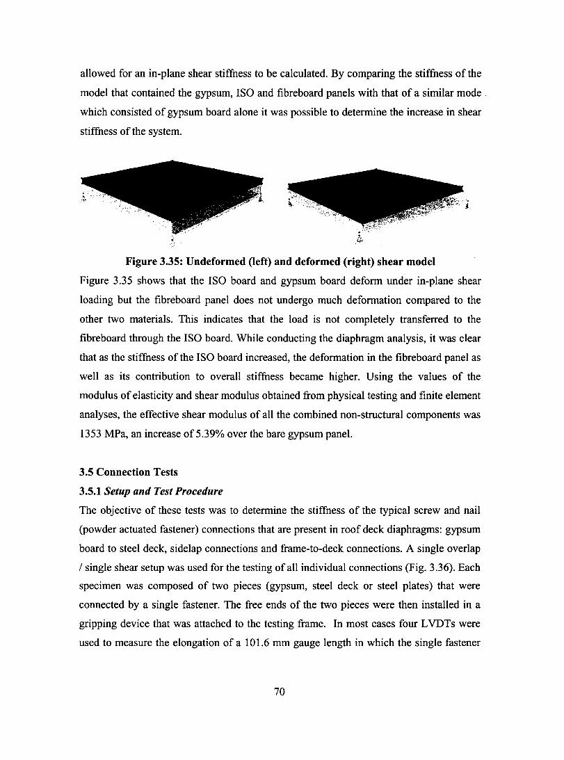
allowed for an in-plane shear stiffness to be calculated. By comparing the stiffness of the
model that contained the gypsum, ISO and fibreboard panels with that of a similar mode .
which consisted of gypsum board al one it was possible to determine the increase in shear
stiffness of the system.
Figure 3.35: Undeformed (left) and deformed (right) shear model
Figure 3.35 shows that the ISO board and gypsum board deform under in-plane shear
loading but the fibre board panel does not undergo much deformation compared to the
other two materials. This indicates that the load is not completely transferred to the
fibreboard through the ISO board. While conducting the diaphragm analysis, it was clear
that as the stiffness of the ISO board increased, the deformation in the fibreboard panel as
weIl as its contribution to overall stiffness became higher. Using the values of the
modulus of elasticity and shear modulus obtained from physical testing and finite element
analyses, the effective shear modulus of all the combined non-structural components was
1353 MPa, an increase of 5.39% over the bare gypsum panel.
3.5 Connection Tests
3.5.1 Setup and Test Procedure
The objective of these tests was to determine the stiffness of the typical screw and nai!
(powder actuated fastener) connections that are present in roof deck diaphragms: gypsum
board to steel deck, sidelap connections and frame-to-deck connections. A single overlap
/ single shear setup was used for the testing of aIl individual connections (Fig. 3.36). Each
specimen was composed of two pieces (gypsum, steel deck or steel plates) that were
connected by a single fastener. The free ends of the two pieces were then installed in a
gripping device that was attached to the testing frame. In most cases four L VDTs were
used to measure the elongation of a 101.6 mm gauge length in which the single fastener
70
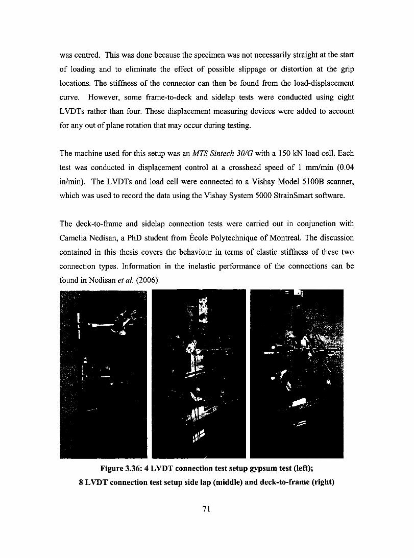
was centred. This was done because the specimen was not necessarily straight at the start
of loading and to eliminate the effect of possible slippage or distortion at the grip
locations. The stiffness of the connector can then be found from the load-displacement
curve. However, sorne frame-to-deck and sidelap tests were conducted using eight
L VDTs rather than foUf. These displacement measuring devices were added to account
for any out of plane rotation that may occur during testing.
The machine used for this setup was an MTS Sintech 30/G with a 150 kN load cell. Each
test was conducted in displacement control at a crosshead speed of 1 mm/min (0.04
in/min). The L VDTs and load cell were connected to a Vishay Model 5100B scanner,
which was used to record the data using the Vishay System 5000 StrainSmart software.
The deck-to-frame and sidelap connection tests were carried out in conjunction with
Camelia Nedisan, a PhD student from École Polytechnique of Montreal. The discussion
contained in this thesis covers the behaviour in terms of elastic stiffness of these two
connection types. Information in the inelastic performance of the connections can be
found in Nedisan et al. (2006).
Figure 3.36: 4 L VDT connection test setup gypsum test (left);
8 LVDT connection test setup side lap (middle) and deck-to-frame (right)
71

3.5.2 Test Specimens
Three types of connections were tested, deck-to-frame, sidelap, and gypsum board-to
deck. A short description of each specimen type is presented in the following sections. As
noted previously each test specimen was constructed of two pieces and a single fastener.
AlI steel test pieces were between 254 mm (10") and 406.4 mm (16") in length. It was
assumed that the length of the piece did not influence the results, because of the L VDT
arrangement which was used to measure the localized deformation around the connector.
The gypsum board pieces were approximately 254 mm (10") in length. In all cases the
connector was installed 50 mm (2") from the end of the overlapped segment of the test
plece.
The sheet steel pieces were fabricated with two 25.4 mm flanges at one end. This was
done because prior testing had shown that without these flanges the end portion of the test
piece would often deform due to the compression loading caused by the test setup. In a
real deck system this buckling is not observed under loading due to the stiffening effect
of the web elements. Hence, these flanges can, in effect, be assumed to represent the
webs of a typical roof deck panel. The gypsum and steel plate pieces were simply
fabricated from either flat panels or bar stock, respectively.
Test specimens were constructed of 0.76 mm, 0.91 mm, 1.22 mm and 1.51 mm ASTM
A653 (2002) Grade 230 MPa sheet steel. The gypsum board was 12.7 mm (112") CGC
Type X, and the steel plates were 4.8 mm (3/16") grade 300W CSAG40.20/G40.21
(1998) material.
3.5.2.1 Deck-to-Frame
Hilti X-ENDK22-THI2 powder actuated (nail) fasteners (Hilti, 2001) were used to
connect the deck elements to the frame (Fig. 3.37). These nails were installed with a
HILTI DX A41 SM tool and the 6.8/11M HILTI #5 short red cartridge. The tool setting
was at the maximum, which allowed for the nail standoffheight limits to be met.
72
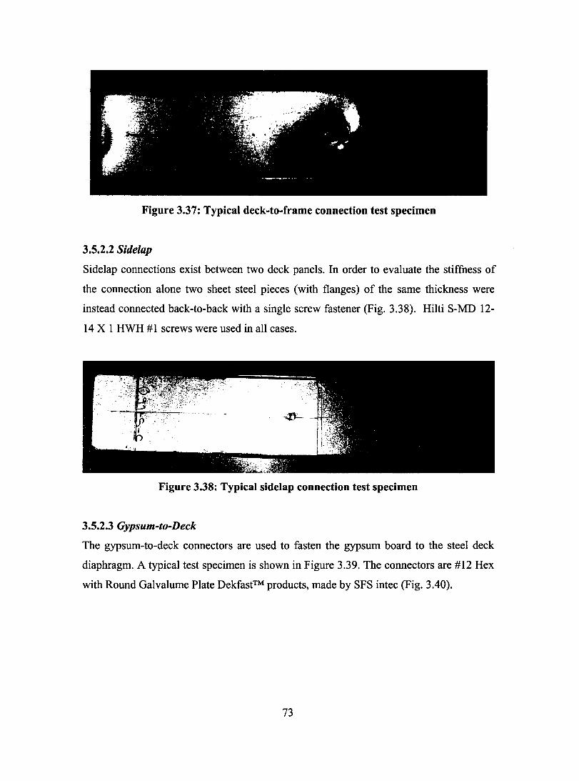
Figure 3.37: Typical deck-to-frame connection test specimen
3.5.2.2 Sidelap
Sidelap connections exist between two deck panels. In order to evaluate the stiffness of
the connection alone two sheet steel pieces (with flanges) of the same thickness were
instead connected back-to-back with a single screw fastener (Fig. 3.38). Hilti S-MD 12-
14 X 1 HWH #1 screws were used in aIl cases.
Figure 3.38: Typical sidelap connection test specimen
3.5.2.3 Gypsum-to-Deck
The gypsum-to-deck connectors are used to fasten the gypsum board to the steel deck
diaphragm. A typical test specimen is shown in Figure 3.39. The connectors are #12 Hex
with Round Galvalume Plate Dekfast™ products, made by SFS intec (Fig. 3.40).
73
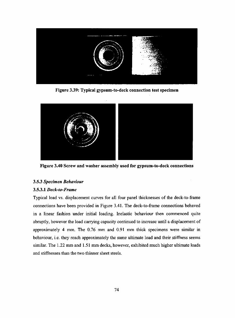
Figure 3.39: Typical gypsum-to-deck connection test specimen
Figure 3.40 Screw and washer assembly used for gypsum-to-deck connections
3.5.3 Specimen Behaviour
3.5.3.1 Deck-to-Frame
Typical load vs. displacement curves for aIl four panel thicknesses of the deck-to-frame
connections have been provided in Figure 3.41. The deck-to-frame connections behaved
in a linear fashion under initial loading. Inelastic behaviour then commenced quite
abruptly, however the load carrying capacity continued to increase until a displacement of
approximately 4 mm. The 0.76 mm and 0.91 mm thick specimens were similar in
behaviour, i.e. they reach approximately the same ultimate load and their stiffness seems
similar. The 1.22 mm and 1.51 mm decks, however, exhibited much higher ultimate loads
and stiffnesses than the two thinner sheet steels.
74

~ "0 ro 0
...J
12000
8000
4000
~--0.76mm
r
---~ 0.91 mm
1.22 mm
1.51 mm
3000
2000
1000 /
-~
/ !
o 0.04 0.08 0.12 0.16 0.2
-' .. _-"', .. --
o ~~-------,---------,---------,----------,---------~------__
o 4 8 12 Displacemenl (mm)
Figure 3.41 Deck-to-frame connection -load vs. displacement
3.5.3.2 Sidelap
Typical load vs. displacement curves for aH four panel thicknesses of the sidelap
connections have been provided in Figure 3.42. As with the deck-to-frame connections,
the behaviour is linear at first and then followed by an inelastic zone. A substantial
increase in capacity is obtained in this inelastic zone for the 1.22 and 1.51 mm thick
specimens; however, this was not the case for the two thinner specimens. Similar to the
deck-to-frame specimens, stiffness and strength increased with the deck thickness.
75
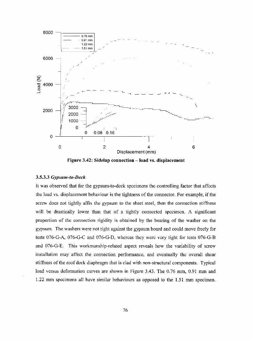
8000
6000
z '-"'
"0 4000 CO 0
--l
2000
0
1
f l'
0
~~~0.76mm
0.91 mm 1.22 mm
1.51 mm
..r"-
2000 1000
0 0
- ...., - "L oh .JI '-...., - - - -I
'-
/'~
.>
h:J
0.08 0.16
1
2 4 Displacement (mm)
Figure 3.42: Sidelap connection -load vs. displacement
3.5.3.3 Gypsum-to-Deck
- '0
\
6
It was observed that for the gypsum-to-deck specimens the controlling factor that affects
the load vs. displacement behaviour is the tightness of the connector. For example, if the
screw do es not tightly affix the gypsum to the sheet steel, then the connection stiffness
will be drastically lower than that of a tightly connected specimen. A significant
proportion of the connection rigidity is obtained by the bearing of the washer on the
gypsum. The washers were not tight against the gypsum board and could move freely for
tests 076-G-A, 076-G-C and 076-G-D, whereas they were very tight for tests 076-G-B
and 076-G-E. This workmanship-related aspect reveals how the variability of screw
installation may affect the connection performance, and eventually the overall shear
stiffness of the roof deck diaphragm that is c1ad with non-structural components. Typical
load versus deformation curves are shown in Figure 3.43. The 0.76 mm, 0.91 mm and
1.22 mm specimens aIl have similar behaviours as opposed to the 1.51 mm specimen.
76

This can be attributed somewhat to the thickness of the sheet steel; however the screw
and washer tightness was more influential on the measured performance.
1600
1200
z ......... "0 800 ctI 0 ~
400
0
---0.76mm
0.91 mm
1.22 mm 1.51 mm
J'
! 0 0.4
/------------. 800
600
400
200
0
0 0.040.080.120.160.2
0.8 1.2 1.6 2 Displacement (mm)
Figure 3.43: Gypsurn-to-deck connection -load vs. displacernent
3.5.4 Data Analysis
The connection stiffness for each of the test specimens was obtained from the slope of the
load versus displacement curve. In most cases, the range between zero load and 40% of
the ultimate load was used to evaluate the stiffuess. However, in sorne instances the
initial portion of the test curve was ignored because of slack and out-of-straightness of
the connection test specimen. Test results for the deck-to-frame, sidelap and gypsum
board-to-deck are listed in Tables 3.6, 3.7 and 3.8, respectively. Table 3.9 contains the
average gypsum board-to-deck connection stiffuess values for those specimens that were
considered to have been adequately constructed, i.e. those which had a tightly installed
screw and washer. The values that were not taken into account had failures modes that
were different from the majority of the specimens.
77

Table 3.6: Deck-to-frame connection stiffness
0.76 mm 0.91 mm Specimen Stiffness Specimen Stiffness
(kN/mm) JkN/mml 076-N-A 36.8 091-N-A 25.9 076-N-B 11.6* 091-N-B 14.1* 076-N-C 32.7 091-N-C 32.1 076-N-D 31.4 091-N-D 16.25* 076-N-E -49.8* 091-N-E 36.2 076-N-H 34.7 091-N-H 57.33* 076-N-1 25.7 091-N-1 32.8
AVERAGE 32.3 AVERAGE 31.7 %COV 13.0% %COV 13.6%
1.22 mm 1.51 mm Specimen Stiffness Specimen Stiffness
(kN/mm) (kN/mm) 122-N-A 47.9 151-N-A 54.2 122-N-B 49.0 151-N-B 49.9 122-N-C 32.0* 151-N-C 36.4* 122-N-D 42.7 151-N-D 43.7 122-N-E 43.6 151-N-E 45.9 122-N-H 50.7 151-N-H 57.6 122-N-1 45.6 151-N-1 40.0*
AVERAGE 46.6 AVERAGE 50.3 %COV 6.7% %COV 11.4%
* Not used in the calculation of average values.
78
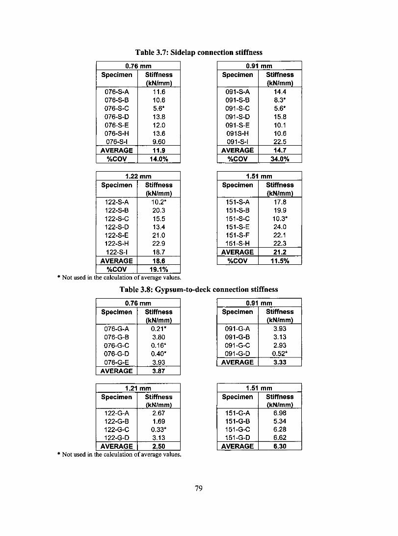
Table 3.7: Sidelap connection stiffness
0.76 mm 0.91 mm Specimen Stiffness Specimen Stiffness
(kN/mm) (kN/mm) 076-5-A 11.6 091-5-A 14.4 076-5-8 10.6 091-5-8 8.3* 076-5-C 5.6* 091-5-C 5.6* 076-5-0 13.8 091-5-0 15.8 076-5-E 12.0 091-5-E 10.1 076-5-H 13.6 0915-H 10.6 076-5-1 9.60 091-5-1 22.5
AVERAGE 11.9 AVERAGE 14.7 %COV 14.0% %COV 34.0%
1.22 mm 1.51 mm Specimen Stiffness Specimen Stiffness
(kN/mm) (kN/mm) 122-5-A 10.2* 151-5-A 17.8 122-5-B 20.3 151-5-B 19.9 122-5-C 15.5 151-5-C 10.3* 122-5-0 13.4 151-5-E 24.0 122-5-E 21.0 151-5-F 22.1 122-5-H 22.9 151-5-H 22.3 122-5-1 18.7 AVERAGE 21.2
AVERAGE 18.6 %COV 11.5% %COV 19.1%
* Not used in the calculation of average values.
Table 3.8: Gypsum-to-deck connection stiffness
0.76 mm 0.91 mm Specimen Stiffness Specimen Stiffness
(kN/mm) (kN/mml 076-G-A 0.21* 091-G-A 3.93 076-G-B 3.80 091-G-B 3.13 076-G-C 0.16* 091-G-C 2.93 076-G-0 0.40* 091-G-0 0.52* 076-G-E 3.93 AVERAGE 3.33
AVERAGE 3.87
1.21 mm 1.51 mm Specimen Stiffness Specimen Stiffness
(kN/mm) (kN/mm)
122-G-A 2.67 151-G-A 6.98 122-G-B 1.69 151-G-B 5.34 122-G-C 0.33* 151-G-C 6.28 122-G-0 3.13 151-G-0 6.62
AVERAGE 2.50 AVERAGE 6.30 * Not used in the calculatlOn of average values.
79
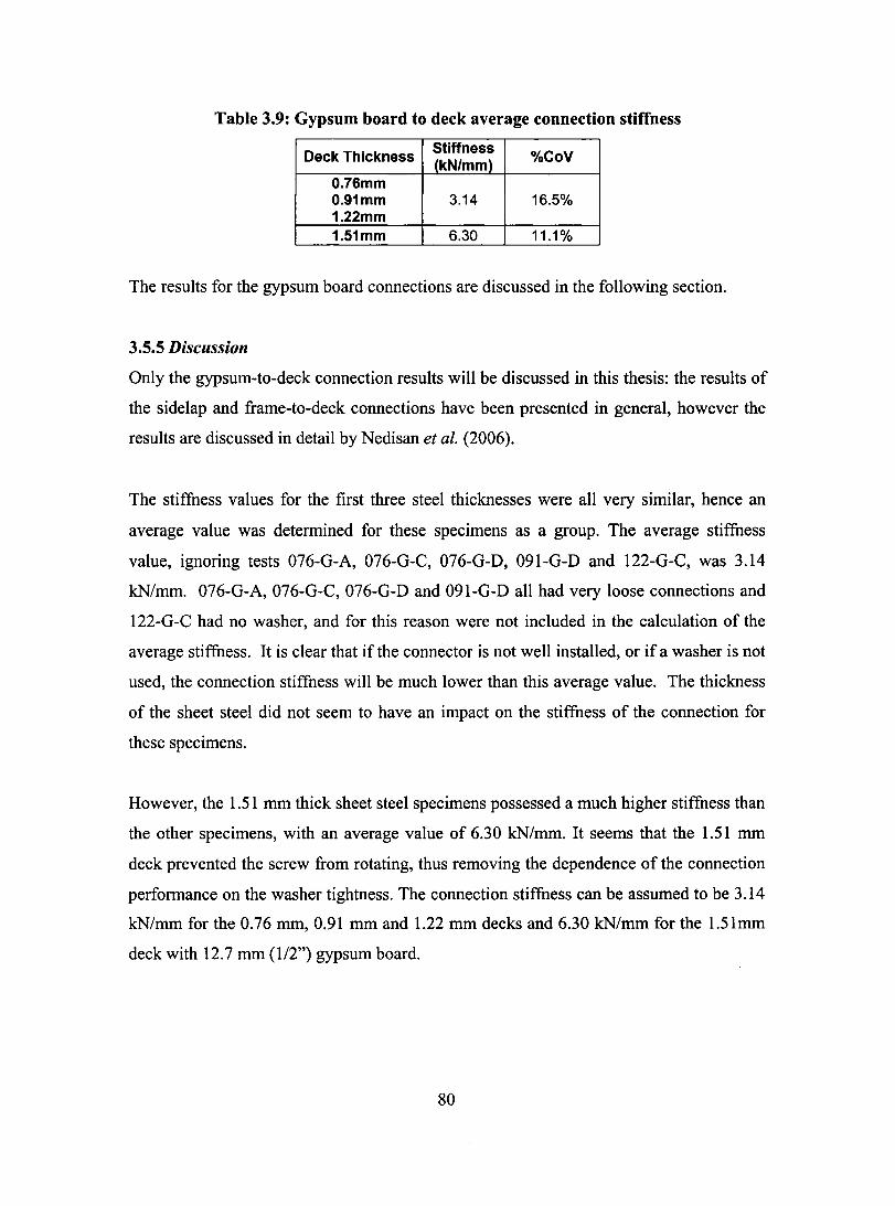
Table 3.9: Gypsum board to deck average connection stiffness
Deck Thickness Stiffness
%CoV (kN/mm) O.76mm O.91mm 3.14 16.5% 1.22mm 1.51mm 6.30 11.1%
The results for the gypsum board connections are discussed in the following section.
3.5.5 Discussion
Only the gypsum-to-deck connection results will be discussed in this thesis: the results of
the sidelap and frame-to-deck connections have been presented in general, however the
results are discussed in detail by Nedisan et al. (2006).
The stiffness values for the first three steel thicknesses were aIl very similar, hence an
average value was determined for these specimens as a group. The average stiffness
value, ignoring tests 076-G-A, 076-G-C, 076-G-D, 091-G-D and 122-G-C, was 3.14
kN/mm. 076-G-A, 076-G-C, 076-G-D and 091-G-D aIl had very 100 se connections and
122-G-C had no washer, and for this reason were not included in the caIculation of the
average stiffness. It is clear that if the connector is not weIl instaIled, or if a washer is not
used, the connection stiffness will be much lower than this average value. The thickness
of the sheet steel did not seem to have an impact on the stiffness of the connection for
the se specimens.
However, the 1.51 mm thick sheet steel specimens possessed a much higher stiffness than
the other specimens, with an average value of 6.30 kN/mm. It seems that the 1.51 mm
deck prevented the screw from rotating, thus removing the dependence of the connection
performance on the washer tightness. The connection stiffness can be assumed to be 3.14
kN/mm for the 0.76 mm, 0.91 mm and 1.22 mm decks and 6.30 kN/mm for the 1.51mm
deck with 12.7 mm (112") gypsum board.
80

3.6 Conclusions
This section contains a review of the results obtained from the experimental material and
connection testing. The stiffness properties that are presented will later be used for the
elastic analyses of diaphragms which is described in Chapter 4. The following
conclusions have been obtained:
1. Cascade 1" Securpan fibreboard: tlexural Young's modulus is 250 MPa and in
plane shear modulus is 235 MPa.
2. Type X 'il" CGC gypsum board: tlexural Young's modulus is 2625 MPa and in
plane shear modulus is 1284 MPa.
3. ISO-board: In-plane shear modulus is 4.0 MPa, obtained from finite element
analysis model.
4. Non-structural roofing section: In-plane shear modulus is 1353 MPa, obtained
from finite element analysis model.
5. Gypsum board-to-steel deck: Connection stiffness for 0.76 mm, 0.91mm and
1.22 mm sheet steel is 3.14 kN/mm; for 1.51 mm sheet steel is 6.31 kN/mm.
6. Frame-to-deck: Connection stiffness for 0.76 mm, 0.91mm, 1.22 mm and
1.51 mm sheet steel are 32.3 kN/mm, 31.7 kN/mm, 46.6 kN/mm and 50.3
kN/mm, respectively.
7. Sidelap: Connection stiffness for 0.76 mm, 0.91 mm, 1.22 mm and 1.51 mm sheet
steel are 11.9 kN/mm, 14.7 kN/mm, 18.6 kN/mm and 21.2 kN/mm, respectively
8. The four-sided shear tests have shown that the small scale shear tests are adequate
to compute the shear stiffness of materials, using equation D-1037a. The test
results in Tables 3.2 and 3.5 are similar for both the gypsum board and fibreboard.
81

CHAPTER4
ELASTIC DIAPHRAGM ANALYSES
4.1 General
The objective of the analytical phase of this research project was to develop linear elastic
finite element analysis models that would adequately reproduce the initial stages of the
roof diaphragm in-plane shear behaviour for different steel panel thicknesses with or
without the presence of non-structural roofing elements. The analytical models, based on
the large-scale diaphragm tests conducted by Yang (2003) (Section 4.2), were built using
the SAP2000 v.8.2.3 software (CSI, 2002). Two models were constructed, using the data
acquired in the experimental stages ofthis project (Chapter 3), to try to reproduce the test
results obtained by Yang of a bare steel diaphragm specimen, as well as a diaphragm that
was constructed with non-structural roofing components. The first model, which was
initially developed by Yang, was modified to suit the context of this research project
(Section 4.3), whereas the second model was built specifically for this research project
(Section 4.4). The data obtained from the analytical models is presented in Section 4.5
along with the computed results. A comparative study of the numerical results with the
SDI calculated stiffness values for multiple connection properties is also provided.
Section 4.6 is dedicated to the discussion of the analytical results.
4.2 Roof Diaphragm Tests by Yang
To understand the finite element models that are presented in this thesis, it is necessary to
first provide an overview of the diaphragm tests conducted by Yang (2003). Yang
carried out twelve large-scale roof diaphragm tests (3.658 m x 6.096 m, 12' x 20'), two of
which were constructed with non-structural components. The following sub-sections
present a description of the test frame and test configurations.
4.2.1 Frame Setup
The test frame used by Yang was identical to that used by Essa et al. (2001) and Martin
(2002). It consisted of a system of pin connected beams and joists (Fig. 4.1), which
represent the framing of a portion of a larger roof structure. The cantilever test frame
82

was constructed of perimeter beams along the edges of the specimen and three joists
spanning the width of the diaphragm.
A Vertical Support
Joist B
t North
o
1... 6096 mm Dog Bones.1
3658 mm
HSS 10 1.6x50.8x4. 78 /Steel Dec
L 100x75xlO
PL 304.8x25.4
Figure 4.1: Plan view of frame setup (Essa et al., 2001)
.1 Figure 4.2: Diaphragm test setup (schematic plan view)
83
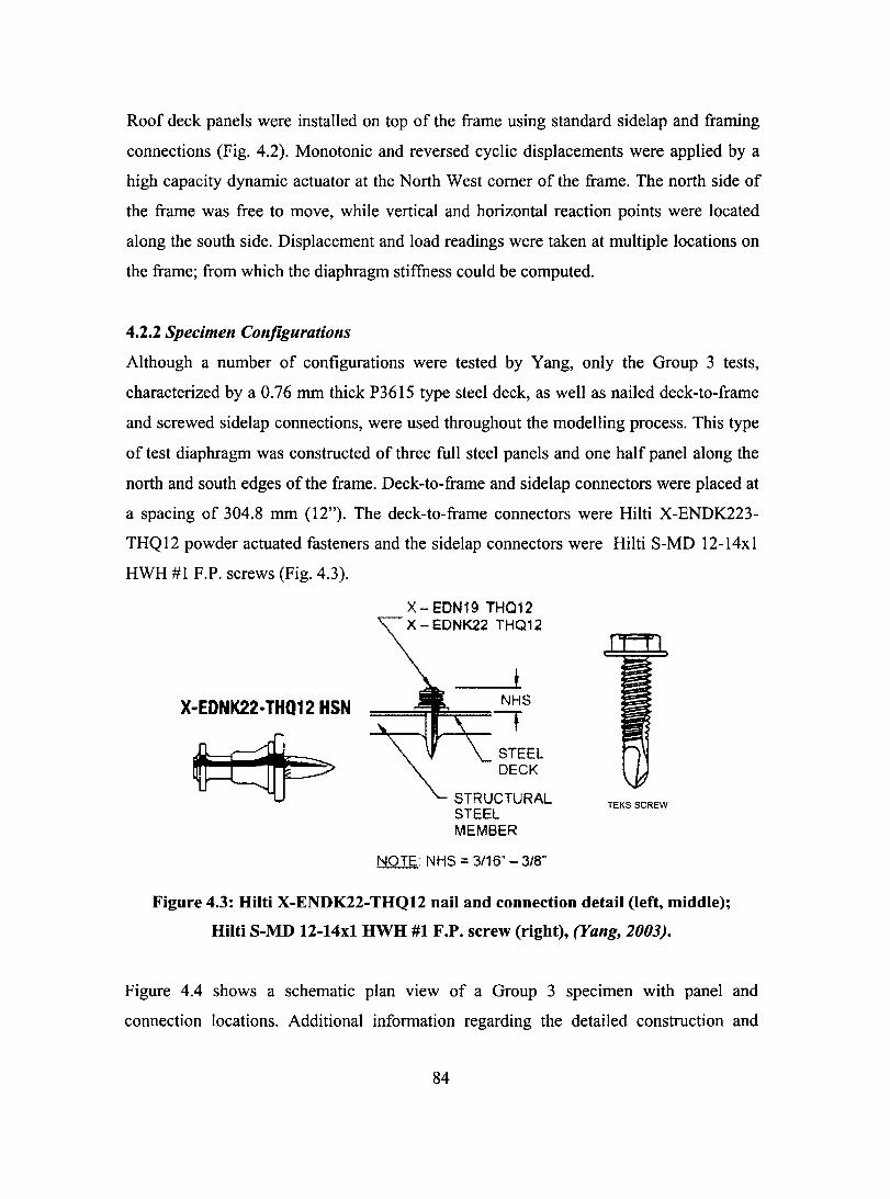
Roof deck panels were installed on top of the frame using standard sidelap and framing
connections (Fig. 4.2). Monotonic and reversed cyclic displacements were applied by a
high capacity dynamic actuator at the North West corner of the frame. The north side of
the frame was free to move, while vertical and horizontal reaction points were located
along the south side. Displacement and load readings were taken at multiple locations on
the frame; from which the diaphragm stiffness could be computed.
4.2.2 Specimen Configurations
Although a number of configurations were tested by Yang, only the Group 3 tests,
characterized by a 0.76 mm thick P3615 type steel deck, as weIl as nailed deck-to-frame
and screwed sidelap connections, were used throughout the modelling process. This type
of test diaphragm was constructed of three full steel panels and one half panel along the
north and south edges of the frame. Deck-to-frame and sidelap connectors were placed at
a spacing of 304.8 mm (12"). The deck-to-frame connectors were Hilti X-ENDK223-
THQ12 powder actuated fasteners and the sidelap connectors were Hilti S-MD 12-14xl
HWH #1 F.P. screws (Fig. 4.3).
X-EDNK22 .. TH012 HSN
X-EDN19 THQ12 X - EDNK22 THQ12
t NHS
~-JIL--~t STEEL DECK
STRUCTURAL STEEL MEMBER
NOTE: NHS = 3/16' -3/8"
TEKS SCREW
Figure 4.3: Hilti X-ENDK22-THQ12 nail and connection detail (Ieft. middle);
Hilti S-MD 12-14x1 HWH #1 F.P. screw (right), (Yang, 2003).
Figure 4.4 shows a schematic plan view of a Group 3 specimen with panel and
connection locations. Additional information regarding the detailed construction and
84

testing procedures, as well as test results, has been documented by Tremblay et al.
(2004), Yang (2003), Martin (2002) and Essa et al. (2001,2003).
Essa developed a nomenclature system which will be used throughout the following
sections. An example of a name for a test specimen is 38-76-6-NS-M, which refers to a
38 mm deep deck, 0.76 mm thick deck, 6 m long specimen (actually 6.1 m, 20'), nailed
deck-to-frame connectors and screwed sidelap connections and monotonic loading.
2 3 4 5 6 7 8 9 10 11 12 13 14 15 16 17 18 19 20 21 • A • • • • • • • • • • • • • • • • • • • • • ~~~' B • • • • • ~,
c
o •
E • • • • • -- --F
;... .• ----* -- -- )(------)(-- -)(-----._ --)(- ~ -)Çr_ .~)t~-.'_. _ •. ==- ._=--=lL-~~~---)(---________ )(-----------)(---~----x - --.. ---" ,
G • • H
J • • K • •
lA
lA
M • •
€ .--'j •
• • • •
• •
• è0
• . · ~ N • • • • • • • • • • • • • • • • • • • ~~~~~~~~~~~~~~~~~~~~~~~~.~~. ~--,
2".1 1.' ]" ]' lI' l, ]' II,)' ! .••. ']' l, ]' 1)' IlrvPi~c 1 1 =42,"'-....... -. 2".'1: "5'+' l -,j~5' -'- 5' r 5' -++', ----""'-----------,(,~-----"----.,f'--------''--------__+_--''''---- " -
. 20'4"
• Sheet to frame connection--Hilti na ils x Side lop connection-Hilti -Screws A-A
Figure 4.4: Plan of Group 3 test layout (Yang, 2003)
Although 49 diaphragms tests have been carried out since 1999, no tests were conducted
with 1.22 and 1.51 mm thick deck. Furthermore, information on diaphragms with non
structural components is limited. Only two tests, both by Yang, included non-structural
components and they had identical rooting assemblies. For the diaphragm tests conducted
with the non-structural components, the rooting material composition was the AMCQ
SBS-34. It is a common roof system composed of the following layers (Fig 4.5) (from top
to bottom):
85

• Two layers (4 mm + 2.2 mm) ofSBS waterproof membrane;
• One layer of 25.4 mm (1") thick non-flammable wood tibreboard, hot bitumen
adhered;
• One layer of 63.5 mm (2.5") thick polyisocyanurate (ISO) insulation, hot bitumen
adhered;
• Two layers ofpaper vapour retarder (No. 15 asphalted felts, hot bitumen adhered;
• One layer of 12.7 mm (1/2") thick gypsum board, 12 screws per panel;
• Steel deck.
\ / 1 \ ' \ ( \ \ f \ ... •
Figure 4.5: Roofing cross-section (Yang, 2003)
Yang (2003) described the gypsum-to-deck fasteners as "[. . .] special screws. Its washer
is made of a 0.46 mm thick galvanized steel dise with a 76.2 mm (3 in.) diameter. The
screw itselfis 4.76 mm in diameter, 41 mm long, with 16 threads per inch long." Figure
4.6 shows the screws, which are produced by SFS Intec as an insulation assembly product
under the name #12 Rex w/ Round Galvalume Plate.
86
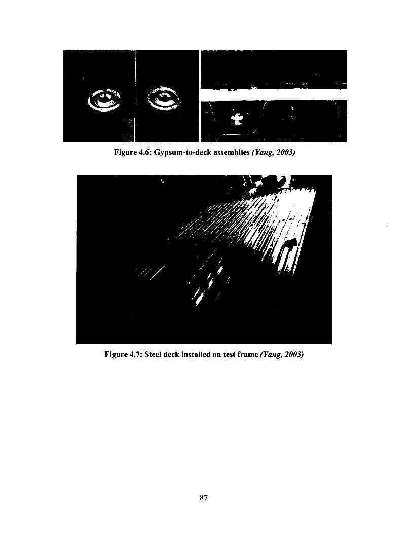
· -.... --~ ---
Figure 4.6: Gypsum-to-deck assemblies (Yang, 2003)
Figure 4.7: Steel deck installed on test frame (Yang, 2003)
87
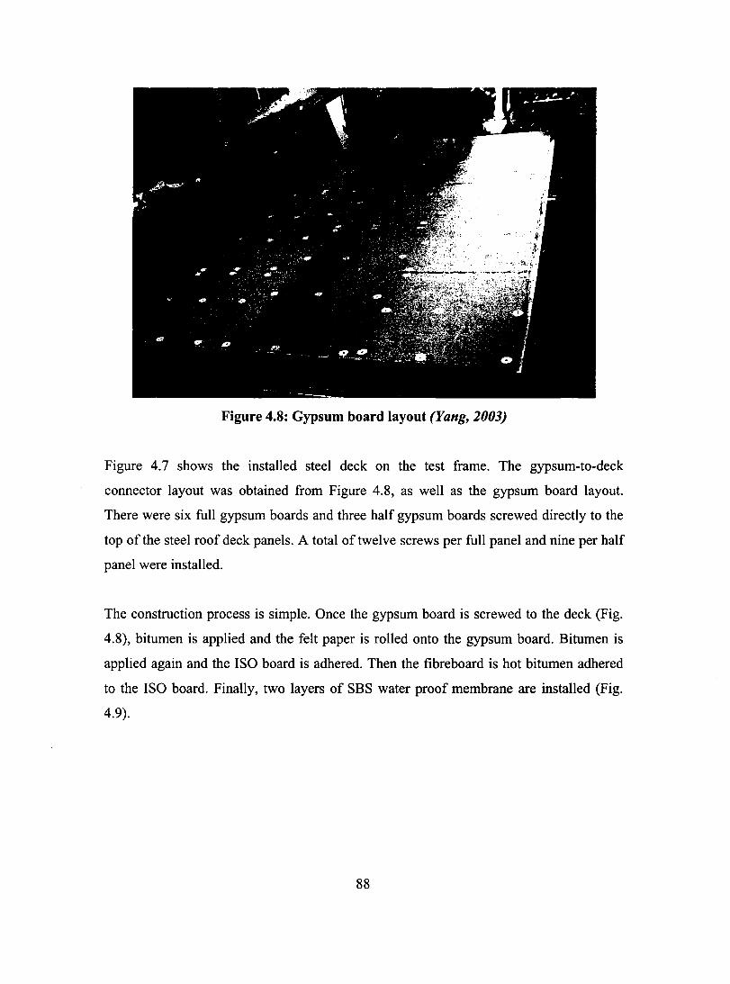
Figure 4.8: Gypsum board layout (Yang, 2003)
Figure 4.7 shows the installed steel deck on the test frame. The gypsum-to-deck
connector layout was obtained from Figure 4.8, as well as the gypsum board layout.
There were six full gypsum boards and three half gypsum boards screwed directly to the
top of the steel roof deck panels. A total of twelve screws per full panel and ni ne per half
panel were installed.
The construction process is simple. Once the gypsum board is screwed to the deck (Fig.
4.8), bitumen is applied and the felt paper is rolled onto the gypsum board. Bitumen is
applied again and the ISO board is adhered. Then the tibreboard is hot bitumen adhered
to the ISO board. Finally, two layers of SBS water proof membrane are installed (Fig.
4.9).
88

Figure 4.9: Roof assembly procedure (Yang, 2003)
4.2.3 Diaphragm Test Results
Group 3 monotonicaHy loaded diaphragm tests 43 and 45 are the two that are of interest
to this study. The first is composed ofa bare sheet steel deck diaphragm (Fig. 4.7) and the
second includes the non-structural components. Subsections 4.2.3.1 and 4.2.3.2 provide a
review of the experimental results for the two deck diaphragms. Table 4.1 shows the
results for aH diaphragm specimens tested by Yang. Specimens 44 and 46 cannot be used
for comparison purposes as the loading protocol was cyclic at a a.5Hz frequency. Thus its
results could only be compared to the SAP model if a similar loading protocol was used,
which is not.
89

T able 4.1: Lar2e-scale diaphraJ m test results (Yang, 200 3)
Test number Test result
GROUP Description Su G' kN/m kN/mm
1 Buildex nail 38 15.25 3.52 39 II.28 1.73
2 Longitudinal overlapped 40 12.68 1.58 41 9.14 1.65 42 10.29 1.55
Bare sheet 43 13.40 2.58 44 10.47 2.85
3 45 15.60 4.17
With roofing 46 15.90 3.90 47 7.27 0.80
4 New profile 48 7.02 0.72 49 8.58 1.06
4.2.3.1 Test 43
As the load increased, the warping defonnation of the panel profile became more and
more extensive (Fig. 4.10). Warping is characterized by the elongation and shortening of
the flutes. Figure 4.11 shows the nonnalized load versus rotation graph. At a load of 75.4
kN (S/Su = 0.92), there was a sudden decrease in capacity due to failure of a deck-to
frame fastener. The load was then distributed to the other adjacent connectors. The
ultimate capacity was 13.40 kN/m and the calculated initial stiffness was 2.58 kN/mm
Figure 4.10: Warping deformation of steel deck profile (Yang, 2003)
90
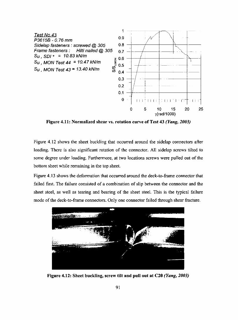
Test No.43 P3615B - 0.76 mm Sidelap fasteners : screwed @ 305 Frame fasteners : Hilti nailed @ 305 Su, SOI * = 10.83 kN/m
1
0.9
0.8
0.7
~ 0.6 ::; Su, MON Test 44 = 10.47 kN/m
Su , MON Test 43 = 13.40 kN/m ~ 0.5
Ci5 0.4
0.3
0.2
0.1
o
---
-
- r------
-
- / - / - / - / - / - Il -
1 1 1 1
o
- --. - ---
r/ '\ I/ v
1\
/ ~~
~"\ Î
1 1 1 1 1 1 1 1 1 1 1 1 1 1 1 1
5 10 15 20 y(rad/1000)
Figure 4.11: Normalized shear vs. rotation curve of Test 43 (Yang, 2003)
-
25
Figure 4.12 shows the sheet buckling that occurred around the sidelap connectors after
loading. There is also significant rotation of the connector. AlI sidelap screws tilted to
sorne degree under loading. Furthermore, at two locations screws were pulled out of the
bottom sheet while remaining in the top sheet.
Figure 4.13 shows the deformation that occurred around the deck-to-frame connector that
failed first. The failure consisted of a combination of slip between the connector and the
sheet steel, as well as tearing and bearing of the sheet steel. This is the typical failure
mode ofthe deck-to-frame connectors. Only one connector failed through shear fracture.
Figure 4.12: Sheet buckling, screw tilt and pull out at C20 (Yang, 2003)
91

4.2.3.2 Test 45
Figure 4.13: Deck-to-frame slip and bearing, tearing
damage of steel sheet at Ill, (Yang, 2003)
The general failure modes for this test were deformation of the steel sheet, the cracking of
the gypsum board, as weIl as the buckling and tearing of the steel sheet around the nails.
Significant warping deformations occurred in the sheet steel, as shown in Figure 4.14,
although this was not as extensive as observed for Test 43. Gypsum-to-deck fasteners
caused the gypsum board to crack (Fig. 4.15). The steel deck pulled the gypsum down,
causing a flexural failure of the gypsum board. No significant deformation was visibly
apparent in the non-structural components other than the gypsum board. Figure 4.16
shows the overall warping and cracking of the gypsum board along its width. No
connector shear failures occurred during the testing of this specimen.
Figure 4.17 shows the normalized load versus rotation graph for test 45. The ultimate
capacity was 15.60 kN/m and the calculated initial stiffness was 4.17 kN/mm.
92

, ". ,
-,-~. i' ,{.
--- -. • dt II .-
- - .. , \ ~
'-",- - ...... ; ......~ ~
Figure 4.14: Steel sheet deformation during loading, fiute width enlarged (left), Steel
sheet deformation during loading, fiute width reduced (right) (Yang, 2003)
Figure 4.15: Steel deck fiute height diminished, gypsum board cracked (Yang, 2003)
Figure 4.16: Warping deformation of steel deck and
cracking of gypsum board - Test 45 (Yang, 2003)
93
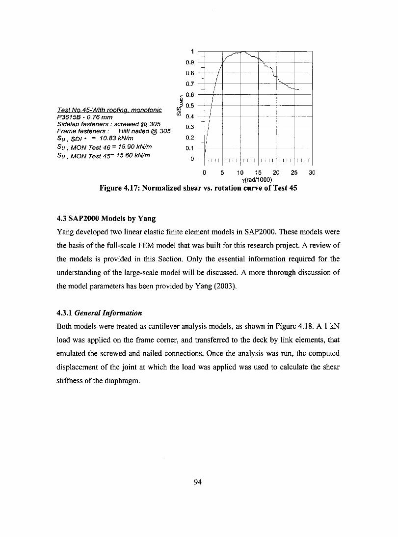
Test No.45-With fOofing. monotonie P3615B - 0.76 mm Sidelap fasteners : serewed @ 305 Frame fasteners : Hilti nailed @ 305 Su, SOI * = 10.83 kN/m Su, MON Test 46 = 15.90 kN/m Su, MON Test 45= 15.60 kN/m
0.9
0.8
0.7
z 0.6 ~
uf 0.5
en 0.4
0.3
0.2
0.1
o
- /" ~ ......,. - / ~ - / "\. - 1 ~ -- 1 - 1
~---- -~. ~--
Il -- ~~.
-
-II - -
-
1111 1111 1111 1111 1111 ,III
o 5 1 0 15 20 25 30 y(rad/1000)
Figure 4.17: Normalized shear vs. rotation curve of Test 45
4.3 SAP2000 Models by Yang
Yang developed two linear elastic finite element models in SAP2000. These models were
the basis of the full-scale FEM model that was built for this research project. A review of
the models is provided in this Section. Only the essential information required for the
understanding of the large-scale model will be discussed. A more thorough discussion of
the model parameters has been provided by Yang (2003).
4.3.1 General Information
Both models were treated as cantilever analysis models, as shown in Figure 4.18. A 1 kN
load was applied on the frame corner, and transferred to the deck by Hnk elements, that
emulated the screwed and nailed connections. Once the analysis was ron, the computed
displacement of the joint at which the load was applied was used to calculate the shear
stiffness of the diaphragm.
94
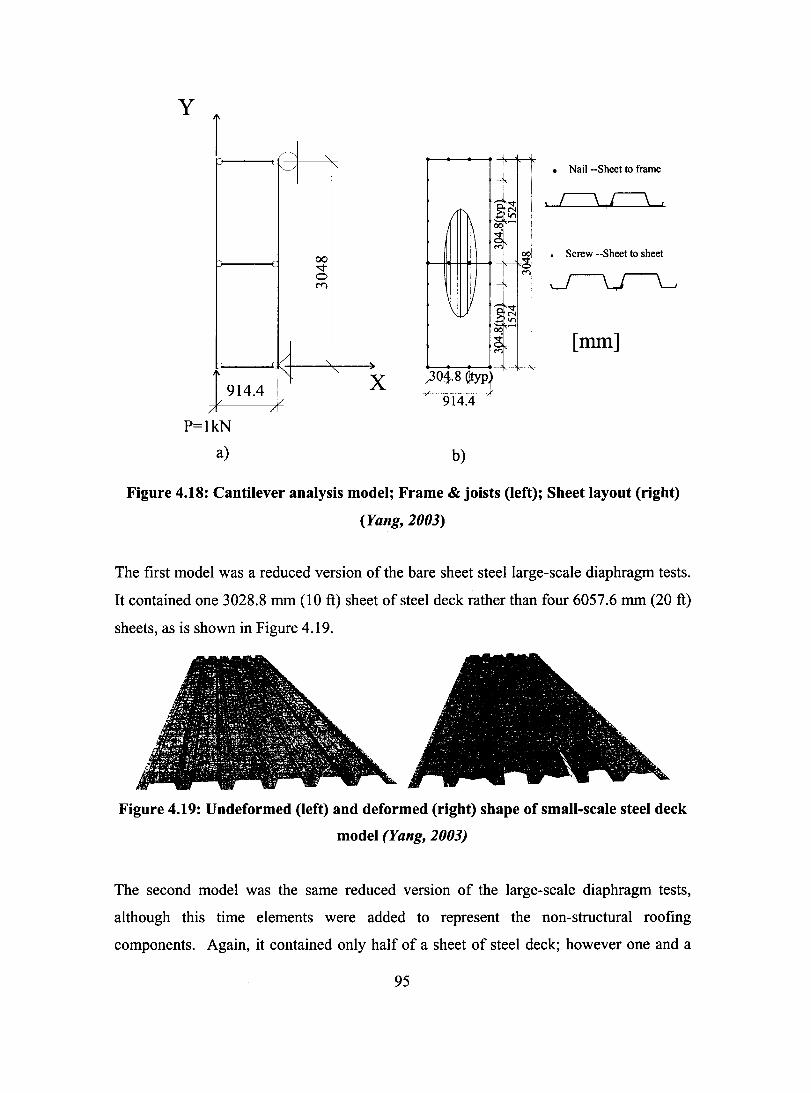
y
,~
J 1 ~/
, C
1 (/ "-
!
]914.4 ,Y P=lkN
a)
"-"- • Naïl --Sheet to frame
00 • Screw --Sheet to sheet
..q-0 M
[mm] "- x J30~.~ ~Pf
914.4
b)
Figure 4.18: Cantilever analysis model; Frame & joists (left); Sheet layout (right)
(Yang, 2003)
The first model was a reduced version of the bare sheet steel large-scale diaphragm tests.
It contained one 3028.8 mm (10 ft) sheet of steel deck rather than four 6057.6 mm (20 ft)
sheets, as is shown in Figure 4.19.
Figure 4.19: Undeformed (left) and deformed (right) shape of small-scale steel deck
model (Yang, 2003)
The second model was the same reduced version of the large-scale diaphragm tests,
although this time elements were added to represent the non-structural roofing
components. Again, it contained only half of a sheet of steel deck; however one and a
95

quarter gypsum boards were added to the previous model rather than the six full boards
and three halfboards (Fig. 4.20). The steel deck sheet was 3048 mm (10') long, whereas
the gypsum boards were only 2438.4 mm (8') long. Therefore a full sheet and a 609.6
mm (2') section were modelled. A gap of 2 mm was placed between the two boards to
avoid contact between the sheets.
Figure 4.20: Undeformed (Ieft) and deformed (right) shape of small-scale steel deck
model with roofing elements (Yang, 1003)
4.3.2 Yang Elements
The steel deck and gypsum board were modelled using shell elements. The shell element
properties were detennined from experimental data acquired through testing and a
literature review done by Yang. The gypsum board thickness was taken as 12.7 mm
(112") and its flexural modulus of elasticity and Poisson's ratio were assumed for this
model, because no data on shear or flexural stiffness was available in the literature.
The screws and nails were modeled using link elements called rubber iso/alors. The link
properties were detennined through testing. These link elements simply act as springs
when a linear static analysis is mn. For this analysis, axial and shear stiffness of the
connections were assigned, however a rotational or bending stiffness were not input.
Finally, link elements called gap elements were inserted in order to prevent the
movement of the gypsum board into the steel deck or of the steel deck into the frame
below. These link elements were present at each joint where there could be contact
between two elements. Figure 4.21 shows a typical gap link element location: joint "i"
96

would be the top of the steel deck and joint "j" would be the bottom ofgypsum board, for
example.
Figure 4.21: Gap property types, shown for axial deformations (CS!, 2002)
The intent is for gap elements to act as "compression only" springs; however, gap
elements are actuaIly linear springs that work both in compression and tension when
simple static linear analyses are run. This was not taken into account when Yang (2003)
carried out his analyses; therefore the gap elements acted as linear springs, not as non
linear link elements. Instead of simply preventing the two elements to coincide, these
elements caused a stiffening of the axial component of the screw connections, which
resulted in a higher stiffness than expected because of added warping rigidity. Proper use
of the gap elements is addressed in the construction of the large-scale model in Section
4.4. Table 4.2 shows aIl the properties that were used in Yang's two finite element
models.
97
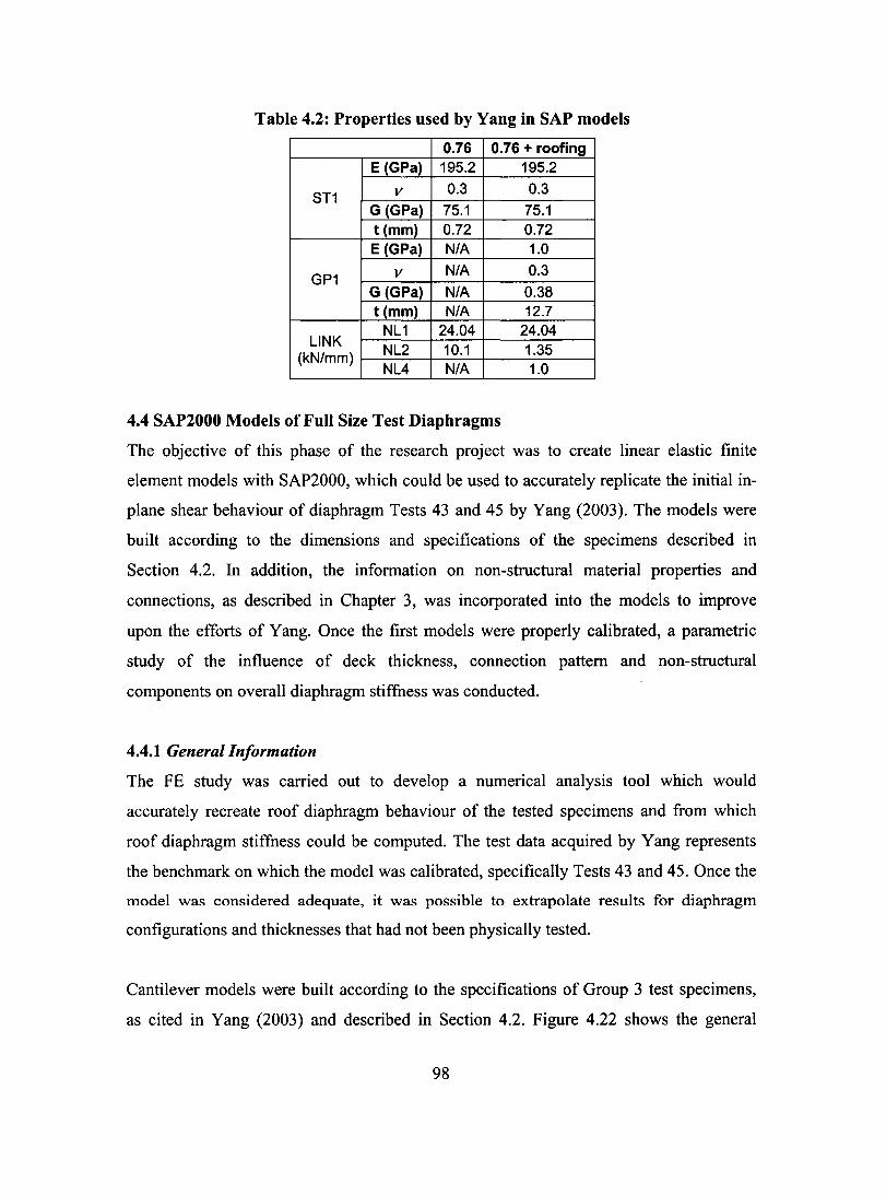
Table 4.2: Properties used by Yang in SAP models
0.76 0.76 + roofing E (GPa) 195.2 195.2
ST1 v 0.3 0.3
G (GPa) 75.1 75.1 t (mm) 0.72 0.72 E (GPa) NIA 1.0
GP1 v NIA 0.3
G (GPa) NIA 0.38 t (mm) NIA 12.7
LlNK NL1 24.04 24.04 NL2 10.1 1.35 (kN/mm) NL4 NIA 1.0
4.4 SAP2000 Models of Full Size Test Diaphragms
The objective of this phase of the research project was to create linear elastic finite
element models with SAP2000, which could be used to accurately replicate the initial in
plane shear behaviour of diaphragm Tests 43 and 45 by Yang (2003). The models were
built according to the dimensions and specifications of the specimens described in
Section 4.2. In addition, the information on non-structural material properties and
connections, as described in Chapter 3, was incorporated into the models to improve
upon the efforts of Yang. Once the first models were properly calibrated, a parametric
study of the influence of deck thickness, connection pattern and non-structural
components on overall diaphragm stiffness was conducted.
4.4.1 General Information
The FE study was carried out to develop a numerical analysis tool which would
accurately recreate roof diaphragm behaviour of the tested specimens and from which
roof diaphragm stiffness could be computed. The test data acquired by Yang represents
the benchmark on which the model was calibrated, specifically Tests 43 and 45. Once the
model was considered adequate, it was possible to extrapolate results for diaphragm
configurations and thicknesses that had not been physically tested.
Cantilever models were built according to the specifications of Group 3 test specimens,
as cited in Yang (2003) and described in Section 4.2. Figure 4.22 shows the general
98

geometry of the model and the steel deck orientation. A total of eight models were
created for this research project: four bare sheet steel roof deck diaphragms with deck
thickness of 0.76 mm, 0.91 mm, 1.22 mm and 1.51 mm, and four roofdeck diaphragms
clad with non-structural components. Additional analyses were carried out while varying
the deck-to-frame and sidelap connector steel deck diaphragms with and without gypsum
board. InitiaIly, the connectors were spaced 305mm (12") apart for both sidelap and
deck-to-frame connectors for aIl four deck thicknesses. Subsequently the spacing was
reduced to 152mm (6"): firstly for the sidelap connectors, then for deck-to-frame
connec tors only, and finally both connector spacings were reduced to 152mm (6"). In aIl,
40 SAP2000 analyses were performed.
The nomenclature used to identify these models was similar to that specified by Essa
(2001). There is one slight difference: a monotonie loading in this case implies a 1 kN
load applied at the corner of the model, not a monotonically increasing load as with a
pushover analysis.
X
/-
"-
-----. ------
// ()
l l ,~~~~~~-n6096~~~~~-7' ,y Figure 4.22: Cantilever analysis model
99

The bare sheet steel model had three full 6.096 m (20') long sheets and two half width
sheets, similar to the tests that were conducted by Yang (2003). The deck-to-frame,
sidelap and gypsum board to steel deck layout is shown in Figures 4.4 and 4.8. The deck
to-frame and sidelap connector spacing was 304.8mm (12"). The model contained 600
frame elements, 17812 shell elements, 1999 link elements and 20456 nodes. Mesh
density was established by Yang (2003). His convergence study showed that his 1592
shell element model was sufficient, therefore the same mesh density was used for this
mode!. The frame elements were restrained in terms of the z-direction translation and for
rotations about x and y. The boundary conditions were continuous for the interior
elements and pinned-tixed for the outer elements. With these boundary conditions, the
frame elements acted as continuous members that were pin connected to one another. The
middle purlins had pinned end connections at the outer elements and continuous at the
inner elements. The frame setup is explained in Section 4.4.2.4 and Figure 4.27 shows the
member end conditions, loading points and supports.
The non-structural rooting component model consisted of the same number of frame
elements, 600, as weIl as 35092 sheIl elements, 1870 link elements and 37264 nodes.
There were less link elements than with the bare sheet steel model in order for a
converged solution to be reached and to reduce computation times. A model was tirst
built with approximately 9000 link elements. Regardless of what parameters were used,
the computations would not converge, even after 1000 steps, with very high convergence
criteria. Therefore "gap" links were inserted at every 152 mm (6") instead of 50.8 mm
(2"), which gave a decent approximation of the real behaviour. A single layer of material
that represented the complete non-structural section was used, not the gypsum board
alone. This is fully explained in Section 4.4.2.
The end conditions of aIl the shell elements were continuous. However, each sheet was
modelled separately such that link elements, which represent the sidelap or deck-to-frame
connections, were needed to connect the various panels and framing members.
100
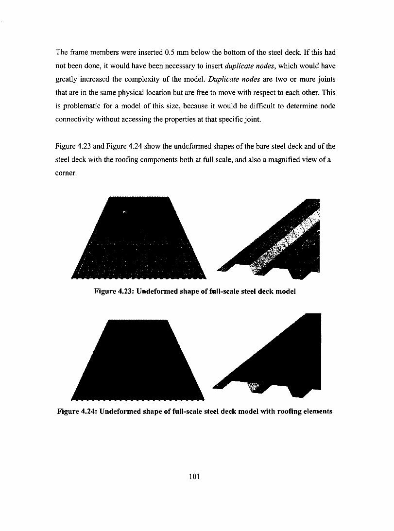
The frame members were inserted 0.5 mm below the bottom of the steel deek. If this had
not been done, it would have been neeessary to insert duplicate nodes, whieh would have
greatly inereased the eomplexity of the mode!. Duplicate nodes are two or more joints
that are in the same physical location but are free to move with respect to eaeh other. This
is problematie for a model of this size, beeause it would be difficult to determine node
eonneetivity without accessing the properties at that specifie joint.
Figure 4.23 and Figure 4.24 show the undeformed shapes of the bare steel deek and ofthe
steel deek with the roofing eomponents both at full seale, and also a magnified view of a
corner.
Figure 4.23: Undeformed shape of full-scale steel deck model
Figure 4.24: Undeformed shape of full-scale steel deck model with roofing elements
101

4.4.2 Elements
Each element in the model is thoroughly discussed in this section. Firstly, the material
properties are presented, followed by shell elements, link elements and finally frame
elements.
4.4.2.1 Material Properties
It was necessary to assign material properties to the frame and shell elements. Two
different material properties were used throughout the analyses: the properties of the steel
were called STI and the non-structural component properties were called OPI.
The STI material properties were taken from the test data compiled in Yang (2003) for
the 0.76 and 0.91 mm thick deck. Since testing of the two thicker deck types has not been
carried out the material properties were defined as prescribed by the CSA S 136 Standard
(2001) for the design of cold-formed steel members. The properties of the non-structural
components (OPl) were taken from the results of the tests presented in Chapter 3.
However, the values that were required for input in SAP2000 were the modulus of
elasticity and Poisson's ratio, not the shear stiffness. The modulus of elasticity (E) in
flexure was known for the gypsum board, as weIl as the shear modulus (0). The
relationship between the flexural modulus of elasticity and shear modulus is described as
for a Hookean material:
E= G 2(1 + v)
where:
E = Flexural modulus of elasticity (MPa),
G = Shear modulus (MPa),
v= Poisson's ratio.
Isolating v in equation (4-1):
(4-1)
102
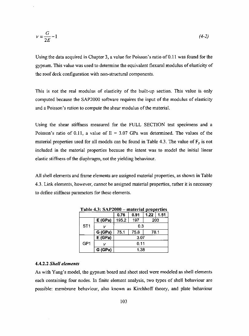
G v=--l
2E (4-2)
Using the data acquired in Chapter 3, a value for Poisson's ratio of 0.11 was found for the
gypsum. This value was used to determine the equivalent flexural modulus of elasticity of
the roof deck configuration with non-structural components.
This is not the real modulus of elasticity of the built-up section. This value is only
computed because the SAP2000 software requires the input of the modulus of elasticity
and a Poisson's ration to compute the shear modulus of the material.
Using the shear stiffuess measured for the FULL SECTION test specimens and a
Poisson's ratio of 0.11, a value of E = 3.07 GPa was determined. The values of the
material properties used for aU models can be found in Table 4.3. The value of Fy is not
included in the material properties because the intent was to model the initial linear
elastic stiffness of the diaphragm, not the yielding behaviour.
An shen elements and frame elements are assigned material properties, as shown in Table
4.3. Link elements, however, cannot be assigned material properties, rather it is necessary
to define stiffness parameters for these elements.
T bl 4 3 SAP2000 a e . . • 1 - matena proper les 0.76 1 0.91 11.22 11.51
E (GPa) 195.2 1 197 1 203 5T1 v 0.3
G (GPa) 75.1 1 75.8 1 78.1 E (Gpa) 3.07
GP1 v 0.11 G (GPa) 1.38
4.4.2.2 Shell elements
As with Yang's model, the gypsum board and sheet steel were modeled as shen elements
each containing four nodes. In finite element analysis, two types of shen behaviour are
possible: membrane behaviour, also known as Kirchhoff theory, and plate behaviour
103
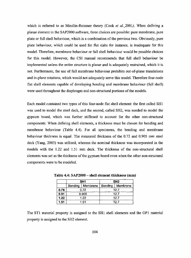
which is referred to as Mindlin-Reissner theory (Cook et al., 2001). When defining a
pl anar element in the SAP2000 software, three choices are possible: pure membrane, pure
plate or full shell behaviour, which is a combination of the previous two. Obviously, pure
plate behaviour, which could be used for flat slabs for instance, is inadequate for this
model. Therefore, membrane behaviour or full shell behaviour would be possible choices
for this model. However, the CSI manual recommends that full shell behaviour be
implemented unless the entire structure is planar and is adequately restrained, which it is
not. Furthermore, the use of full membrane behaviour prohibits out-of-plane translations
and in-plane rotations, which would not adequately serve this model. Therefore four-node
flat shell elements capable of developing bending and membrane behaviour (full shell)
were used throughout the diaphragm and non-structural portions of the models.
Each model contained two types ofthis four-node flat shell element: the first called SHI
was used to model the steel deck, and the second, called SH2, was needed to model the
gypsum board, which was further stiffened to account for the other non-structural
components. When defining shell elements, a thickness must be chosen for bending and
membrane behaviour (Table 4.4). For aIl specimens, the bending and membrane
behaviour thickness is equal. The measured thickness of the 0.72 and 0.905 mm steel
deck (Yang, 2003) was utilized, whereas the nominal thickness was incorporated in the
models with the 1.22 and 1.51 mm deck. The thickness of the non-structural shell
elements was set as the thickness of the gypsum board even when the other non-structural
components were to be modeled.
Table 4.4: SAP2000 - shell element thickness (mm)
SH1 SH2 Bending l Membrane Bending 1 Membrane
0.76 0.72 12.7 0.91 0.905 12.7 1.22 1.22 12.7 1.51 1.51 12.7
The STI material property is assigned to the SHI shell elements and the GPl material
property is assigned to the SH2 element.
104
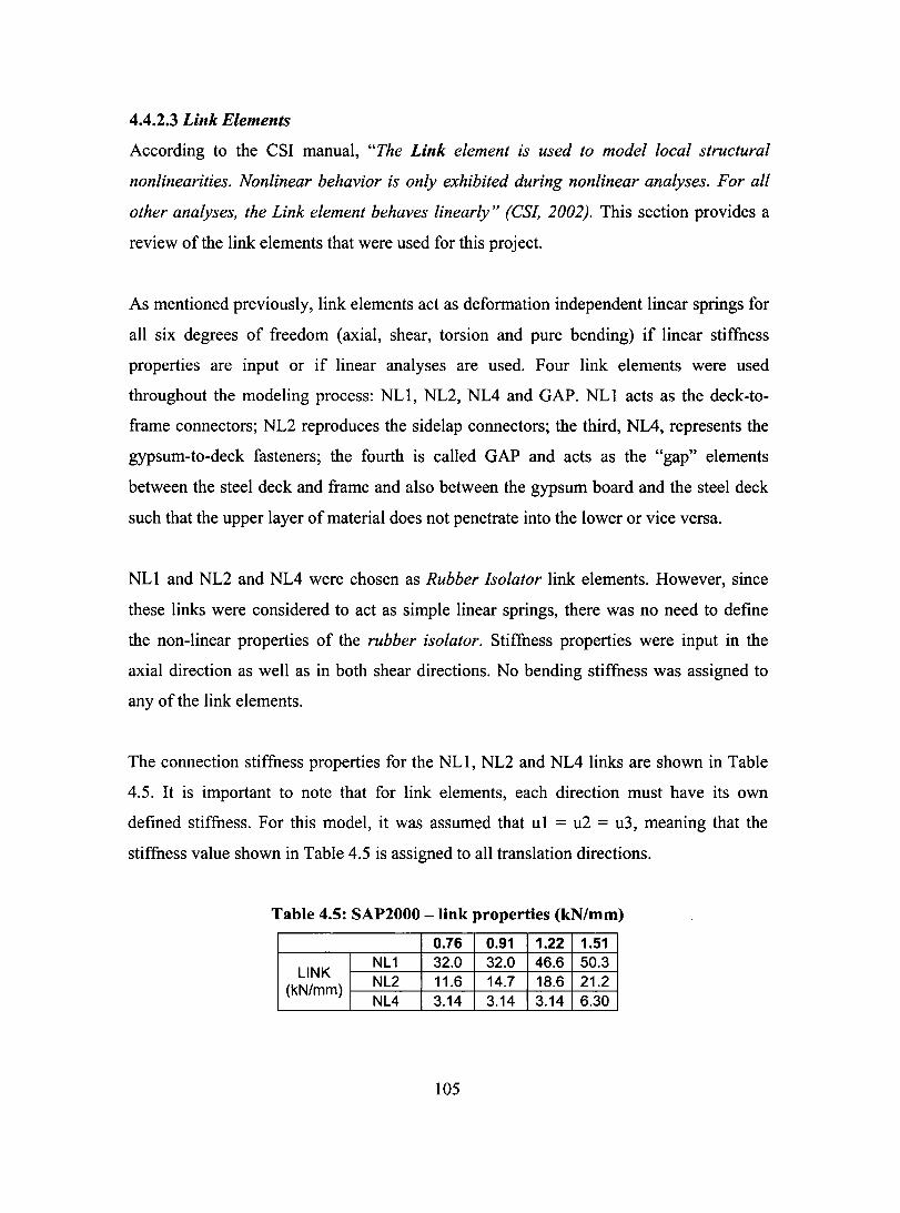
4.4.2.3 Link Elements
According to the CSI manual, "The Link element is used to model local structural
nonlinearities. Nonlinear behavior is only exhibited du ring nonlinear analyses. For al!
other analyses, the Link element behaves linearly" (CSL 2002). This section provides a
review of the link elements that were used for this project.
As mentioned previously, link elements act as deformation independent linear springs for
aIl six degrees of freedom (axial, shear, torsion and pure bending) if linear stiffness
properties are input or if linear analyses are used. Four link elements were used
throughout the modeling process: NL l, NL2, NL4 and GAP. NL 1 acts as the deck-to
frame connectors; NL2 reproduces the sidelap connectors; the third, NL4, represents the
gypsum-to-deck fasteners; the fourth is caIled GAP and acts as the "gap" elements
between the steel deck and frame and also between the gypsum board and the steel deck
such that the upper layer of material does not penetrate into the lower or vice versa.
NL 1 and NL2 and NL4 were chosen as Rubber Isolator link elements. However, since
these links were considered to act as simple linear springs, there was no need to define
the non-linear properties of the rubber isolator. Stiffness properties were input in the
axial direction as weIl as in both shear directions. No bending stiffness was assigned to
any of the link elements.
The connection stiffness properties for the NL l, NL2 and NL4 links are shown in Table
4.5. It is important to note that for link elements, each direction must have its own
defined stiffness. For this model, it was assumed that ul = u2 = u3, meaning that the
stiffness value shown in Table 4.5 is assigned to aIl translation directions.
Table 4.5: SAP2000 - Iink properties (kN/mm)
0.76 0.91 1.22 1.51
LlNK NL1 32.0 32.0 46.6 50.3
(kN/mm) NL2 11.6 14.7 18.6 21.2 NL4 3.14 3.14 3.14 6.30
105
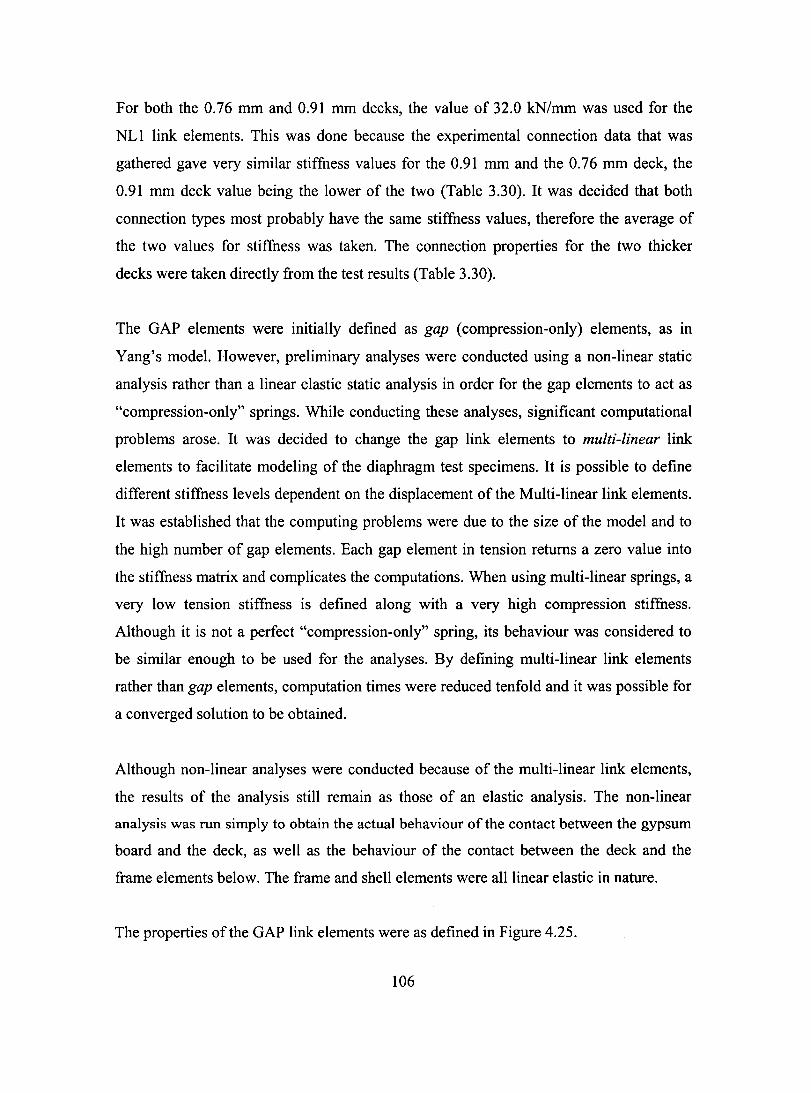
For both the 0.76 mm and 0.91 mm decks, the value of 32.0 kN/mm was used for the
NL 1 link elements. This was done because the experimental connection data that was
gathered gave very similar stiffness values for the 0.91 mm and the 0.76 mm deck, the
0.91 mm deck value being the lower of the two (Table 3.30). It was decided that both
connection types most probably have the same stiffness values, therefore the average of
the two values for stiffness was taken. The connection properties for the two thicker
decks were taken directly from the test results (Table 3.30).
The GAP elements were initially defined as gap (compression-only) elements, as in
Yang's model. However, preliminary analyses were conducted using a non-linear static
analysis rather than a linear elastic static analysis in order for the gap elements to act as
"compression-only" springs. While conducting these analyses, significant computational
problems arose. It was decided to change the gap link elements to multi-linear link
elements to facilitate modeling of the diaphragm test specimens. It is possible to define
different stiffness levels dependent on the displacement of the Multi-linear link elements.
It was established that the computing problems were due to the size of the model and to
the high number of gap elements. Each gap element in tension retums a zero value into
the stiffness matrix and complicates the computations. When using multi-linear springs, a
very low tension stiffness is defined along with a very high compression stiffness.
Although it is not a perfect "compression-only" spring, its behaviour was considered to
be similar enough to be used for the analyses. By defining multi-linear link elements
rather than gap elements, computation times were reduced tenfold and it was possible for
a converged solution to be obtained.
Although non-linear analyses were conducted because of the multi-linear link elements,
the results of the analysis still remain as those of an elastic analysis. The non-linear
analysis was mn simply to obtain the actual behaviour of the contact between the gypsum
board and the deck, as weIl as the behaviour of the contact between the deck and the
frame elements below. The frame and shell elements were aIllinear elastic in nature.
The properties ofthe GAP link elements were as defined in Figure 4.25.
106

80
40
........ z ~ '-" Q) 0 ~ 0 u.
-40
-80
-1.2
~Jacement Force 1 0.01 0 0
-1 -100
1 -0.8 -0.4 0 0.4
Displacement (mm) 0.8
Il 1.2
Figure 4.25: Multi-linear spring stiffness of GAP element
4.4.2.4 Frame Elements
Frame elements are small beam elements with specific cross-sectional properties and
boundary conditions with anode at each end. The element has aIl 6 degrees of freedom,
as it recreates aIl three translations and rotations. The frame elements were used to
recreate the frame setup shown in Figures 4.1 and 4.22. This setup by itself has no in
plane shear stiffness as the members are pin-ended as it is shown in Figure 4.22. Two
frame elements were used throughout: FM 1 and FM2. They have the same cross
sectional properties (Table 4.6), and both are assigned STI material properties. Two
elements were used to differentiate the elements in the X-direction from the elements in
the Y-direction (Figure 4.22). The properties were chosen so that no deformation would
take place in the frame. A test ron was conducted without any steel deck panels to check
for any shear stiffness of the frame setup. It was concluded that the frame setup had no
shear stiffness and very low stresses were present throughout the frame elements.
107

Table 4.6: SAP2000 - frame element properties
FM1 and FM2 Cross-section (axiall area 10000000
T orsional Constant 0 Moment of Inertia about 3 axis 1.00E+10 Moment of Inertia about 2 axis 1.00E+10
Shear area in 2 direction 0 Shear area in 3 direction 0
Section Modulus about 3 axis 0 Section Modulus about 2 axis 0 Plastic Modulus about 3 axis 0 Plastic Modulus about 2 axis 0
Radius of Gyration about 3 axis 0 Radius of G~''ration about 2 axis 0
Figure 4.26 shows a corner of the frame as well as the whole frame outline. As mentioned
previously, the FM2 elements have continuous end connection between each other, but
are pinned when connected to the FM 1, and vice versa for the FM 1 elements.
FM2 • FM2 • FM2
Figure 4.26: Support (lower left); Frame elements and end releases (lower right)
4.4.3 Analysis Parameters
As mentioned above, the analyses were run as non-linear static analyses even though a
linear elastic analysis was actually sought. When running these types of analyses, many
parameters must be defined, including: the number of steps and iterations, convergence
criteria - called lumping tolerances in the SAP2000 software - and the load redistribution
method (hinge unloading method). The maximum number of steps, null steps, iterations
108

per step and the unloading method are the default setting. The incremental displacement
convergence criteria and the load imbalance convergence criteria - called iteration
loading tolerance and event loading tolerance in the SAP2000 software - have been
defined differently than the default values (Table 4.7).
The convergence criteria values were found by trial and error. These values define the
level of precision of the calculation for the incremental displacement as well as for the
load imbalance. As the values for these two parameters increase, the computation time
decreases; as the number of steps needed to arrive to an answer decreases, the results
obtained from the analysis becomes less and less precise. These values must be chosen
with care or the results obtained may be rendered unacceptable. Through a convergence
study, by comparing the calculated results with the physical diaphragm test results for
these models, it was determined that a twelve to fifteen step procedure was necessary to
ensure that the finite element analysis was acceptable.
The hinge unloading option is primarily intended for pushover analysis using frame hinge
properties that exhibit sharp drops in their load-carrying capacity. The "Apply Local
Distribution" setting attempts to imitate how local inertia forces stabilize a rapidly
unloading frame hinge element. However, we are not conducting a SAP2000 pushover
analysis or using frame hinge elements, therefore this option has little effect the model
results but does affect computation tîmes. The "Apply Local Distribution" setting, which
îs considered to be the most effective of all the methods (CS! 2002), was chosen for its
lower computation times for the model used in this research.
Table 4.7: Non-Iinear analysis parameter values
Bare Sheet Steel Model Roofing Model 0.76 0.91 1.22 1.51 0.76 0.91 1.22 1.51
Max. Steps 200 200 200 200 200 200 200 200 Max. Null Steps 50 50 50 50 50 50 50 50
Max. Iterations per Step 10 10 10 10 10 10 10 10 Iteration Convergence Tolerance 0.04 0.04 0.05 0.04 0.01 0.01 0.01 0.01
Event Lumping Tolerance 0.08 0.08 0.10 0.08 0.02 0.01 0.01 0.01
109
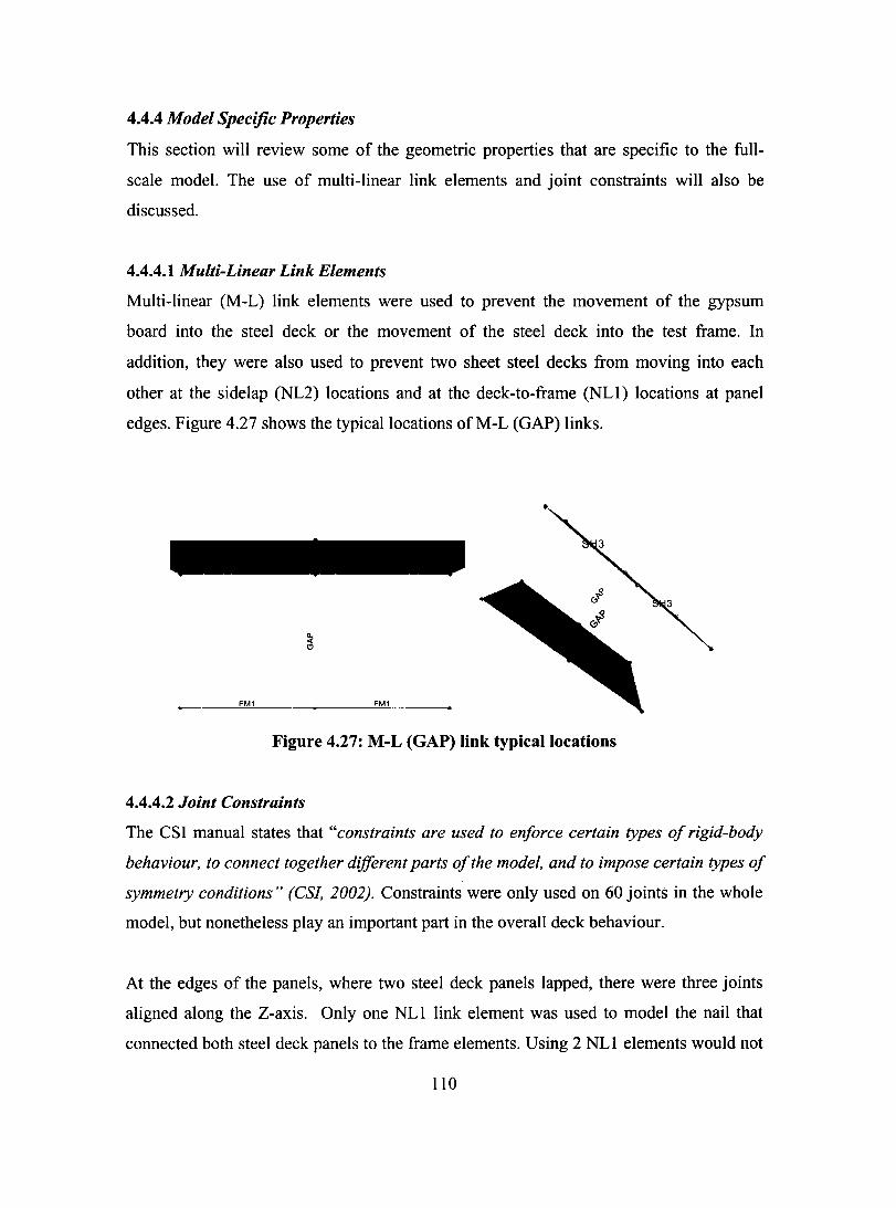
4.4.4 Model Specifie Properties
This section will review sorne of the geometric properties that are specifie to the full
scale mode!. The use of multi-linear link elements and joint constraints will also be
discussed.
4.4.4.1 Multi-Linear Link Elements
Multi-linear (M-L) link elements were used to prevent the movement of the gypsum
board into the steel deck or the movement of the steel deck into the test frame. In
addition, they were also used to prevent two sheet steel decks from moving into each
other at the sidelap (NL2) locations and at the deck-to-frame (NLI) locations at panel
edges. Figure 4.27 shows the typicallocations ofM-L (GAP) links.
FM1 FM1
Figure 4.27: M-L (GAP) link typicallocations
4.4.4.2 Joint Constraints
The CSI manual states that "constraints are used to enforce certain types of rigid-body
behaviour, to connect together difJerent parts of the model, and to impose certain types of
symmetry conditions" (CSL 2002). Constraints were only used on 60 joints in the whole
model, but nonetheless play an important part in the overall deck behaviour.
At the edges of the panels, where two steel deck panels lapped, there were three joints
aligned along the Z-axis. Only one NL 1 link element was used to model the nail that
connected both steel deck panels to the frame elements. Using 2 NLI elements would not
110
have been adequate, because the stiffness would have been double that which existed in a
real roof. Furthermore by using two link elements, unrealistic displacement could occur.
Therefore, a line joint constraint was used to model the behaviour of the nail.
Aline constraint is modeled as equal displacement behaviour for the constrained joints.
Therefore, aIl three joints behave as if they were connected by a straight line, i.e. the two
edge joints move freely while the middle joint movement is controlled by the constraint
conditions. Furthermore, they are also free to move independently in the axial direction
of the constraint. It is adequate to assume this, because deck-to-frame tests have shown
that, except for the 1.51 mm deck, the connection behaviour was controlled by rotation of
the nail and not bending of the nail. Figure 4.28 shows the link element configuration,
where the three joints were assigned with a line constraint. The top and middle nodes
were separated by an M-L link element to prevent movement of the joints into each other.
Only the top and bottom joints were connected with the NL1 link element, which was
used to model the deck-to-frame connections.
Only the top and bottom joints are connected by the link. AlI three joints along the NL1
link are assigned the LINE joint constraint, and therefore the displacement of the middle
joint is govemed by the constraint and the displacement of the top and bottomjoints.
Figure 4.28: NLI link element with 'joint constraint
111
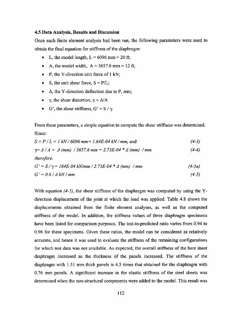
4.5 Data Analysis, ResuUs and Discussion
Once each finite element analysis had been run, the following parameters were used to
obtain the final equation for stiffness of the diaphragm:
• L, the modellength, L = 6096 mm = 20 ft;
• A, the model width, A = 3657.6 mm = 12 ft;
• P, the Y-direction unit force of 1 kN;
• S, the unit shear force, S = P/L;
• IJ., the Y -direction deflection due to P, mm;
• y, the shear distortion, y = /).fA
• G', the shear stiffness, G' = S / "1.
From these parameters, a simple equation to compute the shear stiffness was determined.
Since:
s = P / L = 1 kN /6096 mm= 1. 64E-04 kN / mm, and
r- L1 / A = L1 (mm) /3657.6 mm = 2. 73E-04 * L1 (mm) / mm
therefore,
G' = S / "1 = 164E-04 kN/mm / 2.7 3E-04 * L1 (mm) / mm
G' = 0.6/ L1 kN /mm
(4-3)
(4-4)
(4-5a)
(4-5)
With equation (4-5), the shear stiffness of the diaphragm was computed by using the Y
direction displacement of the joint at which the load was applied. Table 4.8 shows the
displacements obtained from the finite element analyses, as weIl as the computed
stiffness of the model. In addition, the stiffness values of three diaphragm specimens
have been listed for comparison purposes. The test-to-predicted ratio varies from 0.94 to
0.96 for these specimens. Given these ratios, the model can be considered as relatively
accurate, and hence it was used to evaluate the stiffness of the remaining configurations
for which test data was not available. As expected, the overall stiffness of the bare sheet
diaphragm increased as the thickness of the panels increased. The stiffness of the
diaphragm with 1.51 mm thick panels is 4.5 times that obtained for the diaphragm with
0.76 mm panels. A significant increase in the elastic stiffness of the steel sheets was
determined when the non-structural components were added to the model. This result was
112

most evident for the diaphragm with the thinnest steel deck panels. The effect of the non
structural components diminished as the sheet steel thickness increased, i.e. a 58.6%
increase in stiffness was calculated for the 0.76 mm steel, whereas only a 16.9% increase
was obtained for the 1.51 mm panels. Nonetheless, even with the thickest roof deck panel
commonly available on the market, the non-structural components still caused a
substantial increase to the initial elastic stiffness of the diaphragm.
Table 4.8: Analytical model displacements and stiffnesses
Specimen Displacement Stiffness Test Value %Inc %Inc Test/SAP Vs.
(mm) (kN/mm) (kN/mm) Prey. vs. Bare 38-76-6-NS-M 0.219 2.74 2.58 NIA NIA 0.94 38-91-6-NS-M 0.134 4.49 4.22 63.5% NIA 0.94
38-122-6-NS-M 0.072 8.30 NIA 85.0% NIA NIA 38-151-6-NS-M 0.046 13.04 NIA 57.1% NIA NIA 38-76-6-NS-R-M 0.138 4.35 4.17 NIA 58.6% 0.96 38-91-6-NS-R-M 0.093 6.42 NIA 47.7% 43.2% NIA 38-122-6-NS-R-M 0.055 10.85 NIA 68.9% 30.8% NIA 38-151-6-NS-R-M 0.039 15.24 NIA 40.4% 16.9% NIA
Figures 4.29 through 4.32 show the deformed bare steel deck diaphragm and the
deformed shape of the deck with the gypsum board, respectively. The displacement
values listed in Table 4.8 were taken at the bottom left corner of the model at coordinates
(X,Y,Z) = (25.4, 50.8, -0.5).
Figure 4.29: Deformed shape of bare steel deck
113

Figure 4.30 Close-up of warping for bare steel deck
Figure 4.31: Deformed shape of steel deck with roofing components
114

Figure 4.32: Close-up of warping for steel deck with rooting components
As it is shown in Figures 4.29 and 4.30, there is warping in the steel deck, which
corresponds to that observed during testing of the bare steel specimens. The warping
distortion is much less apparent in the model with the non-structural components (Figs.
4.31 & 4.32). Based on observations and the reduced displacement values it can be said
that the non-structural roofing elements limit the extent of deck warping. Figures 4.30
and 4.32 were taken with the same scale factor to amplify the deformations, so a visual
comparison between the two figures is possible. Figure 4.33 shows the flexural
deformation in the non-structural components, as was observed in the diaphragm
specimens tested by Yang (Fig. 4.16). The gypsum board is pulled down at both ends
where NL4 link elements are present. Furthermore, there is no flexural deformation in the
non-structural components over the middle flute because there is no link element.
Figure 4.33: Deformation of non-structural components
115
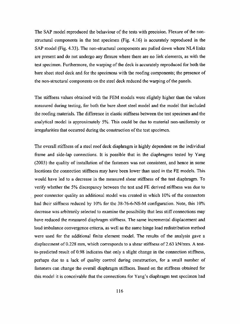
The SAP model reproduced the behaviour of the tests with precision. Flexure of the non
structural components in the test specimen (Fig. 4.16) is accurately reproduced in the
SAP model (Fig. 4.33). The non-structural components are pulled down where NL4 links
are present and do not undergo any flexure where there are no link elements, as with the
test specimen. Furthermore, the warping of the deck is accurately reproduced for both the
bare sheet steel deck and for the specimens with the roofing components; the presence of
the non-structural components on the steel deck reduced the warping of the panels.
The stiffness values obtained with the FEM models were slightly higher than the values
measured during testing, for both the bare sheet steel model and the model that included
the roofing materials. The difference in elastic stiffness between the test specimen and the
analytical model is approximately 5%. This could be due to material non-uniformity or
irregularities that occurred during the construction of the test specimen.
The overall stiffness of a steel roof deck diaphragm is highly dependent on the individual
frame and side-Iap connections. It is possible that in the diaphragms tested by Yang
(2003) the quality of installation of the fasteners was not consistent, and hence in sorne
locations the connection stiffness may have been lower than used in the FE models. This
would have led to a decrease in the measured shear stiffness of the test diaphragm. To
verify whether the 5% discrepancy between the test and FE derived stiffness was due to
poor connector quality an additional model was created in which 10% of the connectors
had their stiffness reduced by 10% for the 38-76-6-NS-M configuration. Note, this 10%
decrease was arbitrarily selected to examine the possibility that less stiff connections may
have reduced the measured diaphragm stiffness. The same incremental displacement and
load imbalance convergence criteria, as weB as the same hinge load redistribution method
were used for the additional finite element mode!. The results of the analysis gave a
displacement of 0.228 mm, which corresponds to a shear stiffness of 2.63 kN/mm. A test
to-predicted result of 0.98 indicates that only a slight change in the connection stiffness,
perhaps due to a lack of quality control during construction, for a small number of
fasteners can change the overall diaphragm stiffness. Based on the stiffness obtained for
this model it is conceivable that the connections for Yang's diaphragm test specimen had
116
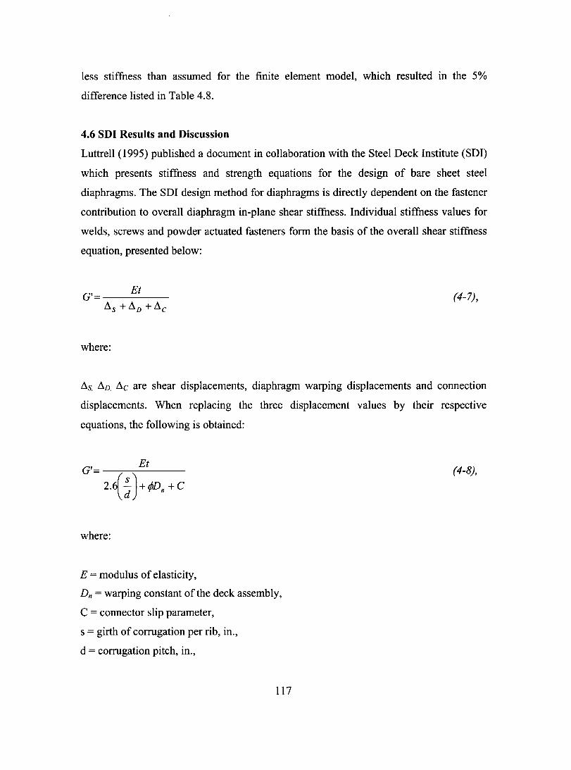
less stiffness than assumed for the finite element model, which resulted in the 5%
difference listed in Table 4.8.
4.6 SDI Results and Discussion
Luttrell (1995) published a document in collaboration with the Steel Deck Institute (SDI)
which presents stiffness and strength equations for the design of bare sheet steel
diaphragms. The SDI design method for diaphragms is directly dependent on the fastener
contribution to overall diaphragm in-plane shear stiffness. Individual stiffness values for
welds, screws and powder actuated fasteners form the basis of the overall shear stiffness
equation, presented below:
Et G'=-----
~S+~D+~C (4-7),
where:
~s. ~D. ~c are shear displacements, diaphragm warping displacements and connection
displacements. When replacing the three displacement values by their respective
equations, the following is obtained:
where:
E = modulus of elasticity,
Dn = warping constant of the deck assembly,
C = connector slip parameter,
s = girth of corrugation per rib, in.,
d = corrugation pitch, in.,
117
(4-8),
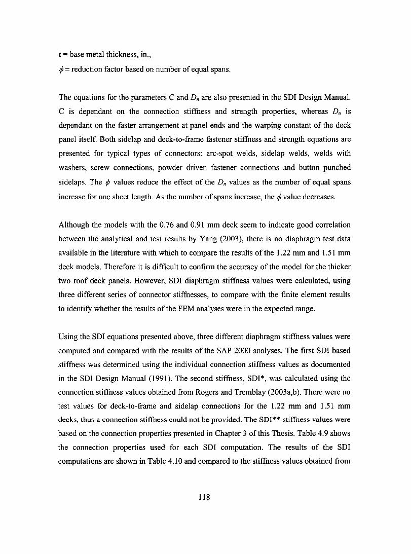
t = base metal thickness, in.,
ljJ = reduction factor based on number of equal spans.
The equations for the parameters C and Dn are also presented in the SDI Design Manual.
C is dependant on the connection stiffness and strength properties, whereas Dn is
dependant on the faster arrangement at panel ends and the warping constant of the deck
panel itself. Both sidelap and deck-to-frame fastener stiffness and strength equations are
presented for typical types of connectors: arc-spot welds, sidelap welds, welds with
washers, screw connections, powder driven fastener connections and button punched
sidelaps. The ljJ values reduce the effect of the Dn values as the number of equal spans
increase for one sheet length. As the number of spans increase, the ljJ value decreases.
Although the models with the 0.76 and 0.91 mm deck seem to indicate good correlation
between the analytical and test results by Yang (2003), there is no diaphragm test data
available in the literature with which to compare the results of the 1.22 mm and 1.51 mm
deck models. Therefore it is difficult to confirm the accuracy of the model for the thicker
two roof deck panels. However, SDI diaphragm stiffness values were calculated, using
three different series of connector stiffnesses, to compare with the finite element results
to identify whether the results of the FEM analyses were in the expected range.
Using the SDI equations presented above, three different diaphragm stiffness values were
computed and compared with the results of the SAP 2000 analyses. The first SDI based
stiffness was determined using the individual connection stiffness values as documented
in the SDI Design Manual (1991). The second stiffness, SDI*, was calculated using the
connection stiffness values obtained from Rogers and Tremblay (2003a,b). There were no
test values for deck-to-frame and sidelap connections for the 1.22 mm and 1.51 mm
decks, thus a connection stiffness could not be provided. The SDI** stiffness values were
based on the connection properties presented in Chapter 3 ofthis Thesis. Table 4.9 shows
the connection properties used for each SDI computation. The results of the SDI
computations are shown in Table 4.10 and compared to the stiffness values obtained from
118
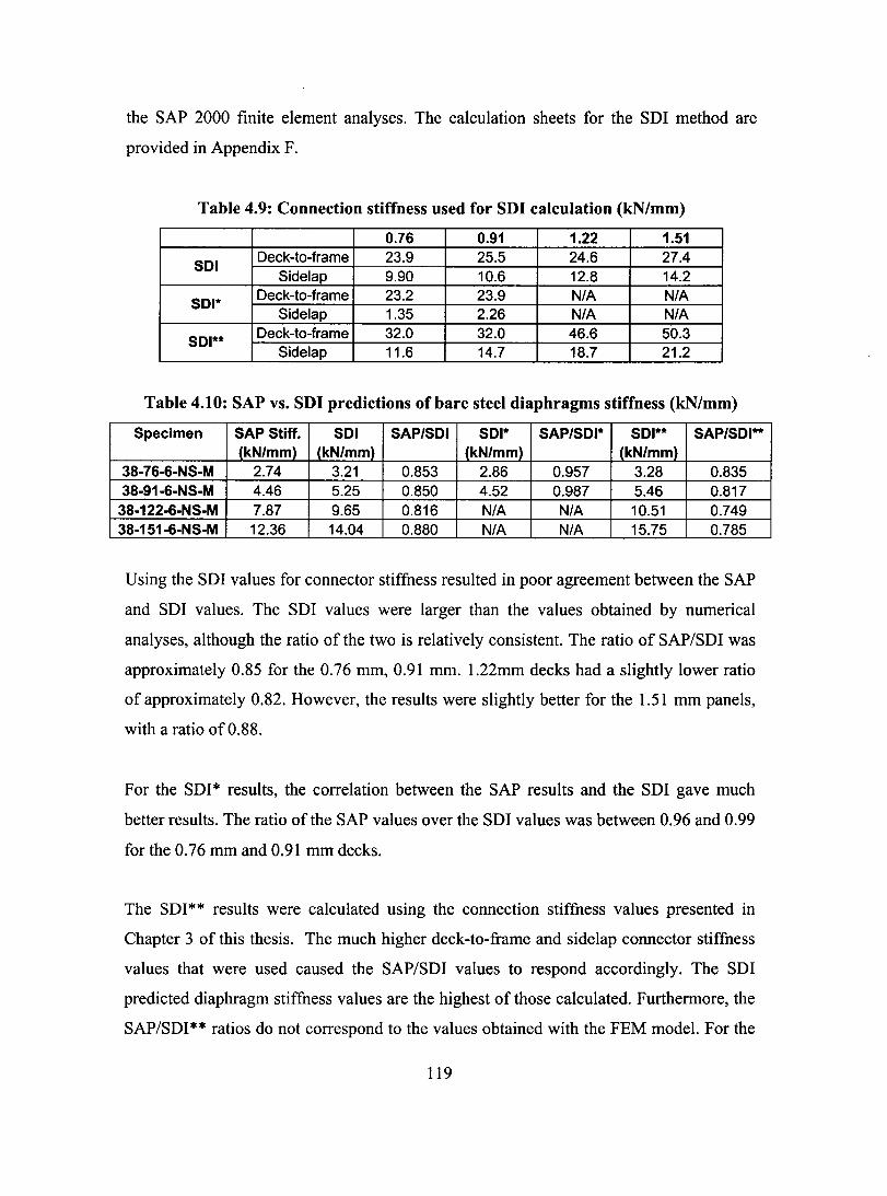
the SAP 2000 finite e1ement analyses. The calculation sheets for the SDI method are
provided in Appendix F.
Table 4.9: Connection stiffness used for SDI calculation (kN/mm)
0.76 0.91 1.22 1.51
SOI Deck-to-frame 23.9 25.5 24.6 27.4
Sidelap 9.90 10.6 12.8 14.2
501* Deck-to-frame 23.2 23.9 NIA NIA
Sidelap 1.35 2.26 NIA NIA
501** Deck-to-frame 32.0 32.0 46.6 50.3
Sidelap 11.6 14.7 18.7 21.2
Table 4.10: SAP vs. SDI predictions of bare steel diaphragms stiffness (kN/mm)
Specimen SAP Stiff. SOI SAP/SOI 501* SAP/SOI* 501** SAP/SOI** (kN/mm) (kN/mm) (kN/mm) (kN/mm)
38-76-6-NS-M 2.74 3.21 0.853 2.86 0.957 3.28 0.835 38-91-6-NS-M 4.46 5.25 0.850 4.52 0.987 5.46 0.817 38-122-6-NS-M 7.87 9.65 0.816 NIA NIA 10.51 0.749 38-151-6-NS-M 12.36 14.04 0.880 NIA NIA 15.75 0.785
Using the SDI values for connector stiffness resulted in poor agreement between the SAP
and SDI values. The SDI values were larger than the values obtained by numerical
analyses, although the ratio of the two is relatively consistent. The ratio of SAP/SDI was
approximate1y 0.85 for the 0.76 mm, 0.91 mm. 1.22mm decks had a slightly lower ratio
of approximately 0.82. However, the results were slightly better for the 1.51 mm panels,
with a ratio of 0.88.
For the SDI* results, the correlation between the SAP results and the SDI gave much
better results. The ratio of the SAP values over the SDI values was between 0.96 and 0.99
for the 0.76 mm and 0.91 mm decks.
The SDI** results were calculated using the connection stiffness values presented in
Chapter 3 of this thesis. The much higher deck-to-frame and sidelap connector stiffness
values that were used caused the SAP/SDI values to respond accordingly. The SDI
predicted diaphragm stiffness values are the highest of those calculated. Furthermore, the
SAP/SDI** ratios do not correspond to the values obtained with the FEM model. For the
119
lighter panels, the ratio is approximately 0.82, but for the two thicker panels, the ratios
are 0.749 and 0.785 for the 1.22 mm and 1.51 mm decks respectively.
The results presented above show that the SDI results consistently overestimate the
stiffness values of the deck diaphragms. Regardless of the combination of stiffness values
used, the model results were much lower than the SDI values obtained. Because the SDI*
values are the closest to the SAP analysis values and the values obtained by Yang (2003),
it seems clear that the connection properties calculated by Rogers and Tremblay
(2003a,b) are more accurate than the values predicted by the SDI equations.
In light of these results, it is safe to assume the finite element model adequately estimates
diaphragm behaviour of thicker decks. The consistency with which the model
overestimates the SDI values points to a realistic estimation of deformations of the steel
deck diaphragms for thicker steel panels.
However, the analysis was run with a 1 kN point load only. The behaviour of this model
is most likely non-linear. The interaction between the gypsum board and the steel deck is
likely to change as deformations in the steel deck increase due to higher loads. As the
load increases, the shear stiffness of the diaphragm may decrease because of this
interaction. Further analyses should be run, using higher loading values.
4.7 Influence of Non-Structural Components on Diaphragm Stiffness: Parametric
Study
The goal of this parametric study was to determine the contribution of the non-structural
components to overall roof diaphragm in-plane shear stiffness for different sheet steel
thicknesses and, more importantly, connection configurations using SDI values of deck
to-frame and sidelap connector stiffness. Designers commonly rely on SDr connection
stiffness values to calculate steel deck diaphragm stiffness and capacity, therefore this
series of analyses was conducted to identify the possible impact that non-structural
components may have on SDI calculated G' values.
120

The findings in the previous Section seem to point to a significant contribution to shear
stiffness by the non-structural components, although the effect of structural connector
spacing is unknown. The purpose of this study was to explore the effects of deck-to
frame and sidelap connector layouts on non-structural component contribution to overall
in-plane diaphragm shear stiffness. In addition, it was previously found that the gypsum
board provided for most of the increase in diaphragm shear stiffness, and that the
remaining non-structural components were for the most part ineffective in changing G' of
the overall roof system. For this reason the properties of the non-structural e1ements in
the models used for the parametric study were defined based on the gypsum panels alone.
4.7.1 General Information
A total of 32 analyses were carried out for this study, comprising of four different steel
deck thicknesses - 0.76, 0.91, 1.22 and 1.51 mm - and four structural connector
configurations, with and without the gypsum board. Two spacings are typically used in
construction for the deck-to-frame and sidelap connectors of a roof diaphragm: 305 mm
and 152 mm. This study consisted of four connector spacing combinations: 305/305,
305/152, 152/305 and 152/152, where the first number is the deck-to-frame connector
spacing and the second is the sidelap connector spacing, in millimetres. Although sorne
minor changes were made to the FE models for these parametric study analyses, the
elements and analysis settings were defined as for the previous models (Sections 4.4 &
4.5).
Given that the finite element analysis of the shear test model in Section 3.4.5.2 indicated
that the actual contribution of the ISO board and fibreboard to the stiffness of the non
structural sandwich to be bare1y over 5%, it was decided that the material properties of
the non-structural components for these analyses would be the shear modulus and
modulus of elasticity of the gypsum board alone. Therefore, the SH2 shell element was
defined to have values of 2625 MPa for the modulus of elasticity (E) and 1284 MPa for
the shear modulus (G).
121

4.7.2 SDI Connector Stiffness
The SDI equations for deck-to-frame and sidelap connectors were used to calculate the
values for the connector stiffnesses. These deck-to-frame and sidelap values were used in
the SAP model for the NLI and NL2 link elements respectively (Table 4.11). There are
no equations or values provided for the gypsum-to-deck connector stiffness in the
literature, therefore the data acquired in Chapter 3 was used for the NL4 elements, as was
done for the previous models.
Table 4.11: SAP -link properties (kN/mm)
0.76 0.91 1.22 1.51 NL 1 19.42 21.25 24.60 27.37
L1NK NL2 10.10 11.05 12.79 14.23 (kN/mm) NL4 3.14 3.14 3.14 6.28
4.7.3 Results
Using the connector stiffness values shown in Table 4.11 in conjunction with the four
nominal deck thicknesses and four connector configurations, diaphragm shear stiffness
values were obtained for bare steel deck diaphragms and for diaphragms with a gypsum
board layer (Table 4.12). The percentage increase in diaphragm stiffness due to the
addition of the gypsum board is tabulated in Table 4.13 for aIl sixteen of the diaphragms
that were modelled.
Table 4.12: SAP - diaphragm stiffness G' (kN/mm)
Bare Steel With Roofing 305/305 305/152 152/305 152/152 305/305 305/152 152/305 152/152
0.76 3.26 4.05 9.29 11.84 4.78 5.59 10.71 13.25 0.91 5.17 5.40 12.35 15.51 6.46 7.06 13.71 16.88 1.22 8.51 8.70 17.39 23.06 10.05 10.15 18.74 24.36 1.51 12.55 13.11 22.32 30.05 13.82 14.42 23.76 31.47
Table 4.13: Increase in G' stiffness with gypsum board
305/305 305/152 152/305 152/152 0.76 46.4% 38.1% 15.3% 11.9% 0.91 25.0% 30.6% 11.0% 8.8% 1.22 18.1% 16.7% 7.8% 5.6% 1.51 10.1% 10.0% 6.5% 4.7%
122
The results clearly indicate a trend: as the steel diaphragm becomes stiffer due to either
the use of a thicker deck or more closely spaced structural connections, the contribution
of the gypsum board to overall diaphragm stiffness decreases on a percentage basis. For
the 0.76 mm specimen with a 305/305 connector spacing, a significant increase in G'
(46.4 %) was caused by the addition of the gypsum layer. Conversely, for the 1.51 mm
specimen with a 152/152 spacing, the increase was less than 5%. However, when
comparing G' values for bare diaphragms versus diaphragms with the gypsum board, the
actual contribution of the non-structural layer is very similar in absolute terms for aIl of
the configurations modeled. The increase in shear stiffness between the diaphragm with
the gypsum board and the bare sheet steel diaphragm varied between 1.27 and 1.65
kN/mm, with an average value of 1.41 kN/mm and a Co V of 7.6%. These results indicate
that the structural connector layout does not influence the non-structural component
contribution to in-plane shear stiffuess of a roof diaphragm.
In summary, it was possible to recreate the diaphragm test results in a realistic fashion
through the use of a finite element model. The contribution to overall diaphragm shear
stiffness of the non-structural components diminishes on a percentage basis as the overall
stiffness of the bare sheet steel deck increases. Furthermore, the absolute contribution of
the gypsum remains relatively constant, regardless of connector spacing or thickness of
the roof deck panels.
123
CHAPTER5
CONCLUSION AND RECOMMENDATIONS
5.1 Conclusions
The overall goal of this research was to provide a better understanding of the effect of
non-structural rooting components on the performance of single-storey steel buildings
subjected to seismic loading, specitically on roof diaphragm behaviour. This has been
achieved by means of materials tests, tinite element analyses and a comparative study of
predicted diaphragm and stiffness values.
Firstly, series of experiments were conducted to evaluate the shear and flexural stiffness
values of the non-structural components in a roof assembly, as well as the stiffness of the
deck-to-frame, sidelap, and gypsum-to-deck connectors. In total, 171 tests were
conducted: 9 small scale shear tests, 68 flexural tests, 22 large scale shear tests and 72
connection tests.
From these tests, the following data was acquired:
• Cascade Securpan tibreboard: Young's modulus in flexure is 250 MPa and in
plane shear stiffness is 235 MPa,
• Type X 12.7 mm (W') CGC gypsum board: Young's modulus in flexure is 2625
MPa and in-plane shear stiffness is 1284 MPa,
• ISO board: in-plane shear stiffness is calculated as 4.0 MPa, from the tinite
element analysis,
• AMCQ SBS-34 rooting system: In-plane shear stiffness is 1353 MPa, from the
tinite element analysis,
• Gypsum board to steel deck connection: connection stiffness for 0.76, 0.91 and
1.22 mm deck is 3.14 kN/mm; for 1.51 mm sheet steel is 6.30 kN/mm,
• Deck-to-frame: connection stiffness for 0.76, 0.91, 1.22 and 1.51 mm deck are
32.3,31.7,46.6 and 50.3 kN/mm, respectively,
• Sidelap: connection stiffness for 0.76, 0.91, 1.22 and 1.51 mm deck are 11.6,
14.7, 18.6 and 21.2 kN/mm, respectively,
124
• Small scale shear tests are adequate to compute the shear stiffness of materials
with the ASTM D1073a equation, although non-isotropic materials could give
multiple results.
It can be seen from the test data that the gypsum board is the stiffest element of the non
structural components, and because of this has the greatest influence on the in-plane
force-deformation behaviour of the steel roof deck diaphragm. The other non-structural
elements, either due to their low in-plane shear stiffness or lack of a direct connection to
the steel deck, do not have as much of an effect.
A finite element model was developed using SAP2000 to analyse the linear elastic
behaviour of bare sheet steel deck diaphragms and diaphragms constructed with non
structural roofing components. The material and connection test data was input into the
finite element model, and a comparison of the measured stiffness of three diaphragm
specimens tested by Yang (2003) and Essa et al. (2000) was carried out. The stiffness
results of analyses 38-76-6-NS-M, 38-91-6-NS-M and 38-76-6-NS-R-M correlated weIl
to the measured values, with test-to-predicted ratios in the range of 0.94 to 0.96. Given
the close agreement of the test and analytical results it was concluded that the finite
element model is adequate for the prediction of the linear elastic behaviour of roof deck
diaphragms.
A study was then carried out in which the elastic stiffness of five additional roof
diaphragms with varying configuration was evaluated with the finite element model. Test
data for diaphragms of these configurations was not available. In general, the diaphragm
stiffness increased as the thickness of the steel roof deck panels increased. Furthermore,
the contribution of the non-structural components, in terms of an increase in in-plane
shear stiffness, was apparent for aIl deck thicknesses. This increase in stiffness became
less on a percentage basis as the deck thickness was increased. As an example, for the
0.76 mm deck, the increase in stiffness due to the non-structural roofing components was
approximately 58.6% compared with a 16.9% increase for the 1.51 mm deck.
125

At this point, the stiffness resuIts that were obtained by the finite element model were
compared to three sets of SDI predicted values: SDI, SDI* and SDI**. SDI was
calculated using the SDI values for connection stiffness, SDI** with the connection
stiffness values obtained from Rogers and Tremblay (2003a,b) and SDI** with the
connection property values presented in Chapter 3 of this Thesis. The SDI values gave
consistently higher stiffnesses than the SAP models, for all three SDI resuIts. However,
the best convergence was obtained with SDI*.
To explain the 5% over-stiffness obtained using the SAP models, the 38-78-6-NS-M
model was tested with 10% of its sidelap and deck-to-frame connectors at 90% of their
original stiffness. The results of the analysis showed that the diaphragm shear stiffness
decreased from 2.74 to 2.63 kN/mm. The Test/SAP ratio went from 0.94 to 0.98, which
shows that an overestimate of the connection stiffness or a faulty installation of even a
small percentage of connectors might be the cause of the higher stiffness in the SAP
model than in the test diaphragms. However, as was discussed in Chapter 4, the event and
iteration lumping tolerances play an important role with respect to the accuracy of the
analysis results. Therefore, it is possible that the use of lower lumping tolerances would
retum more adequate results.
A parametric study was conducted in order to determine the contribution of gypsum
board to overall in-plane shear stiffness of the steel deck diaphragm, with multiple deck
thicknesses and connector layouts. For these FE models the stiffness of the sidelap and
deck-to-frame connectors was based on the SDI predicted values, not test results. The
study showed that the contribution of the gypsum board remained relatively constant
regardless of deck thickness and connector spacing. On average, the diaphragm with the
gypsum board was 1.41 kN/mm stiffer than the equivalent bare diaphragm. Moreover, the
percentage increase in shear stiffness of the diaphragm became less as the deck thickness
was increased and as the structural connectors were placed at a closer spacing.
As stated in Chapter 2, Medhekar (1997) and Tremblay et al. (1995, 2000) have shown
that diaphragm stiffness influences the natural period of buildings to a large extent.
126
Therefore, non-structural roofing elements, when gypsum board is used, should be
considered in the overall in-plane diaphragm stiffness when calculating the natural period
of vibration.
5.2 Recommendations
This study has shown that the gypsum board has a much higher shear stiffness than the
other non-structural components considered. From this finding, it can be assumed that
the contribution of the non-structural components to the roof diaphragm stiffuess would
be significantly less if the gypsum board were not present.
One of this project's objectives was to accurately determine the in-plane shear stiffness
properties of the non-structural components. The values obtained in Chapter 3 using the
finite element analysis model of the four sided shear test specimen confirm that the shear
stiffness of the AMCQ SBS-34 roof system is greater than that of the gypsum board
alone. The SAP2000 analyses were run with the shear modulus determined with the
simplifying equation of the concentric load. Although additional SAP2000 analyses could
be carried out with the new shear stiffness values for the non-structural components, the
change in predicted diaphragm deformations would be minor.
To better understand the contribution of non-structural components to overall structure
behaviour, inelastic analyses of diaphragms including the non-structural components
should be conducted.
Furthermore, a broader database of test information should be compiled for diaphragms
constructed of 1.22 and 1.51 mm decks. Although the results of the SAP analyses of 0.76
and 0.91 mm decks showed good agreement with the diaphragm tests, the 1.22 and 1.51
mm decks have not been tested and their predicted behaviour cannot be confirmed.
Moreover, performing a finite element analysis to determine the diaphragm in-plane
shear stiffness is tedious and time consuming. The development of empirical equations to
127

account of the contribution of the non-structural components to diaphragm in-plane shear
stiffness or the addition of a term to the SDI equations should be carried out.
Lastly, the values obtained for diaphragm stiffness should be introduced into the
equations developed by Medhekar (1997) and Tremblay (2005) to find new predictions
for the natural periods of single storey steel buildings, which could be compared with the
data acquired by Ventura and Turek (2005) and Lamarche (2005). This comparison
should shed light on the actual influence of roof deck diaphragm stiffness on overall
building period of vibration.
128

REFERENCES
AMERICAN SOCIETY FOR TESTING AND MATERIALS, A653 (2002), Standard
Specifications for Steel Sheet, Zinc-Coated (galvanized) or Zinc-Iron Alloy-Coated
(Galvannealed) by the Hot-Dip Process., Philadelphia, PA, USA.
AMERICAN SOCIETY FOR TESTING AND MATERIALS, C203 (1999), Standard
Test Methods for Breaking Load and Flexural Properties of Block-Type Thermal
Insulation. West Conshohocken, PA, USA.
AMERICAN SOCIETY FOR TESTING AND MATERIALS, C473 (1997), Standard
Test Methods for Physical Testing of Gypsum Panels Products. West Conshohocken, PA,
USA.
AMERICAN SOCIETY FOR TESTING AND MATERIALS, DI037 (1999). Evaluating
the Properties of Wood-Base Fibre and Particle Panel Materials. West Conshohocken,
PA, USA.
AMERICAN SOCIETY FOR TESTING AND MATERIALS, D2719 (1989, Reapproved
1994). Standard Test Methods for Structural Panels in Shear Through-the-Thickness.
West Conshohocken, PA, USA.
AMERICAN SOCIETY FOR TESTING AND MATERIALS, D3043 (1995)., Standard
Methods of Testing Structural Panels in Flexure. West Conshohocken, PA, USA.
AMERICAN SOCIETY FOR TESTING AND MATERIALS, E455 (2002), Test Method
for Static Load Testing of Framed Floor or Roof Diaphragm Construction for Buildings.,
West Conshohocken, PA, USA.
BAKER, M.C., (1980), Roofs----Design, Application and Maintenance., Sponsored by
the National Research Council of Canada, Montréal, Qc., Canada.
129

BÉRAIR, T., (1999), Étude expérimentale sur le comportement sismique de bâtiments
d'un seul étage en acier avec diaphragme de toit flexible., École Polytechnique de
Montréal, Montréal, Qc., Canada.
BOUDREAULT, F.A., (2005), Seismic Analysis of Steel Frame / Wood Panel Shear
Walls., Masters Thesis, Department of Civil Engineering and Applied Mechanics, McGill
University, Montréal, Qc., Canada.
CANADIAN SHEET STEEL BUILDING INSTITUTE, (1991), Design of Steel Deck
Diaphragms., BI3-91, Cambridge, Ont. Canada.
CANADIAN STANDARDS ASSOCIATION, CSA, (2004), AI23.4, Asphalt for
Construction of Built-Up Roof Coverings and Waterproofing Systems., Etobicoke, Ont.,
Canada.
CANADIAN STANDARDS ASSOCIATION, CSA, (1992), CAN/CSA-G40.20/G40.21-
92, General Requirements for Rolled or Welded Structural Ouality Steel/Structural
Ouality Steels., Etobicoke, Ont. Canada.
CANADIAN STANDARDS ASSOCIATION, CSA, (1994), CAN/CSA-SI6. Limit
States Design of Steel Structures. Etobicoke, Ont., Canada.
CANADIAN STANDARDS ASSOCIATION, CSA, (2001), CAN/CSA-SI6. Limit
States Design of Steel Structures. Etobicoke, Ont., Canada.
CANAM (1999). Steel deck. Canam Manac Gr., www.canammanac.com.
CARR, A.J., (2000), Ruaumoko - Inelastic Dynamic Analysis., Version March 15th
2000. Dept. Of Civil Eng., University of Canterbury, Christchurch, New Zealand.
130

COMPUTERS AND STRUCTURES, !Ne. (2002). SAP2000 Version 8.0, Integrated
Finite Element Analysis and Design of Structures. Berkeley, CA, USA.
COOK, R.D., MALKUS, D.S., PLESHA, M.E., WITT, R.J., (2001), Concepts and
Applications of Finite Element Analysis., Fourth Edition, Jon Wiley & Sons, Inc. New
York, NY, USA.
ESSA, H.S., TREMBLAY, R., ROGERS, C.A., (2001), Inelastic Seismic Behaviour of
Steel Deck Roof Diaphragms Under Oasui-static Cyclic Loading., Report no. EPM/CGS-
2001-11. Department of Civil, Geologiccal and Mining Engineering, École Polytechnique
de Montréal, Montréal, Qc., Canada.
ESSA, H.S., TREMBLAY, R., ROGERS, C.A., (2003), Behaviour of Roof Deck
Diaphragms Under Ouasi-Static Cyclic Loàding., Journal of Structural Engineering,
ASCE, Vol. 129 No. 12, 1658-1666.
FEDERAL EMERGENCY MANAGEMENT AGENCY, FEMA, (1997),
FEMA2731274, Guidelines for the Seismic Rehabilitation of Buildings., Washington,
District of Columbia, USA.
HIL TI, (2001), Hilti North America. Product Technical Guide-200 1 Edition., Hilti
Corporation, Schaan, Principality of Liechstenstein.
LAMARCHE, e.P., (2005), Étude Expérimentale du comprtement Dynamique des
Bâtiments de Faible Hauteur en Acier., Masters Thesis, Dept. of Civil Engineering,
Université de Sherbrooke, Sherbrooke, Qc., Canada.
LUTTRELL, L.D., (1995), Steel Deck Institute Design Manual., Second Edition,
Department of Civil Engineering, West Virginia University, Morgantown, WV, USA.
131
MARTIN, E., (2002), Inelastic Response of Steel Roff Deck Diaphragms Under
Simulated Dynamically Applied Seismic Loading., Masters Thesis, Dept. Of Civil,
Geological and Mining Engineering, École Polytechnique de Montréal, Montréal, Qc.,
Canada.
MEDHEKAR, M.S., (1997), Seismic Evaluation of Steel Buildings with Concetrically
Braced Frames., Ph.D. in Structural Engineering thesis, Department of Civil and
Environmental Engineering, University of Alberta, Edmonton, Alberta, Fall, 1997.
MEDHEKAR, M.S., KENNEDY, D.J.L., (1999), Seismic Evaluation of Single-Storey
Buildings., Canadian Journal of Civil Engineering, 26, p.379-394.
NEDISAN, C.D., MASTROGIUSEPPE, S., TREMBLAY, R., ROGERS, C.A., (2006),
Shear tests on HILTI nailed frame and screwed side-Iap fasteners for 0.76 to 1.52 mm
thick cold-formed sheet steel., Research Report No.EPMlCGS-2006-1, Department of
Civil, Geological and Mining Engineering, École Polytechnique, Montréal, Canada.
NEDISAN, C., (2002), Comportement Sismique de Bâtiments d'un Seul Étage en Acier
avec Diaphragme de Toit Flexible., Masters Thesis, Dept. of Civil, Geological and
Mining Engineering, École Polytechnique de Montréal, Montréal, Qc., Canada.
NILSON, A.H., (1960), Shear Diaphragm of Light Gage Steel., Journal of the Structural
Division, Proceedings of the American Society of Civil Engineers, Vol. 86, No. STll,
p.111-139.
NRCC, (1995), National Building Code of Canada 1995 CNBCC)., Ilth ed .. Canadian
Commission on Building and Fire Codes, National Research Council of Canada, Ottawa,
Ontario, Canada.
132
NRCC, (2005), National Building Code of Canada 2005 (NBCC)., 12th ed .. Canadian
Commission on Building and Fire Codes, National Research Council of Canada, Ottawa,
Ontario, Canada.
ROGERS, c.A., TREMBLAY, R., (2000), Inelastic Seismic Response of Frame and
Sidelap Fasteners of Steel Roof Decks., Research Report No. EPM/CGS-2000-09,
Department of Civil, Geological and Mining Engineering, École Polytechnique de
Montréal, Montréal, Qc., Canada.
ROGERS, C.A., TREMBLAY, R., (2003a), Inelastic Seismic Response of Sidelap
Fasteners for Steel Roof Deck Diaphragms., Journal of Structural Engineering, ASCE,
Vol. 129 No12, p.1637-1646.
ROGERS, C.A., TREMBLAY, R., (2003b), Inelastic Seismic Response of Frame
Fasteners for Steel Roof Deck Diaphragms. Journal of Structural Engineering, ASCE,
Vol. 129 No. 12, p.1647-1657
ROGERS, c.A., TREMBLAY, R., YANG, W., MARTIN, E., (2004). Ductile design of
steel roof deck diaphragms for earthquake resistance. Proceeding of the 13 th W orld
Conference on Earthquake Engineering, Paper N 0.1997.
STEEL DECK INSTITUTE, SDI, (1981), Diaphragm Design Manual., Canton, OH,
USA.
STEEL DECK INSTITUTE, SDI, (1991), Diaphragm Design Manual., Second Edition,
Canton, OH, USA.
TREMBLAY, R., BÉRAIR, T., (1999), Shake table testing of low-rise steel buildings
with flexible roof diaphragms. Proceedings of the 8th Canadian Conference on
Earthquake Engineering, Vancouver, Canada. 585-590.
133
TREMBLAY, R. AND STIEMER, S.F. (1996), Seismic behaviour of single-storey steel
structures with flexible diaphragm. Canadian Journal of Civil Engineering, Vol. 23: 49-
62.
TREMBLAY, R., (2005), Fundamental Period of Vibration of Braced Steel Frames for
Seismic Design., Earthquake Spectra 2005, August, Vol.21 No.3, p.831-861.
TREMBLAY, R., et al., (2000), Experimental Behaviour of Low-Rise Steel Buildings
with Flexible Roof Diaphragms., Proceeding of the 12th World Conference on
Earthquake Engineering, Auckland, NZ. Paper No. 2567.
TREMBLAY, R., et al., (2004), Experimental investigation and dynamic simulation of
low-rise steel buildings for efficient seismic design., 13th World Conference on
Earthquake Engineering, Paper No.2919.
TREMBLAY, R., ROGERS, C.A., MARTIN, E., YANG, W., (2004). Analysis. Testing and
Design of Steel Roof Deck Diaphragms for Ductile Earthquake Resistance., Journal of
Earthquake Engineering, Vol. 8 No. 5, 775-816.
TREMBLAY, R., STIEMER, S.F., (1996), Use of Uniform Hazard Spectrum and
Computed Period in the Seismic Design of Single-Storey Steel Structures., Proceedings
ofthe 7th U.S. National Conference on Earthquake Engineering, Boston, MA, USA.
TUREK, M., VENTURA, C., (2005), Ambient Vibration of Low-Rise Buildings with
Flexible Diaphragms., Proceedings of the 23rd International Modal Analysis Conference,
Orlando, FL, USA, Februrary 2005, Paper 304.
VENTURA, C., (1995), Ambient Vibration test of the Safeway Store., report by the UBC
Ambient Vibration Team, Dept. of Civil Engineering, University of British Columbia,
Vancouver, BC, Canada.
134

VINSON, J.R., (1999), The Behaviour of Sandwich Structures of Isotropic and
Composite Materials., Technomic Publishing Co., Lancaster, PA, USA.
YANG, W., (2003), Inelastic Seismic Response of Steel Roof Deck Diaphragms
Including Effects of Non-Structural Components and End Laps., Masters Thesis, Dept.
Of Civil, Geological and Mining Engineering, École Polytechnique de Montréal,
Montréal, Qc., Canada.
135

APPENDIXA
TWO-SIDED SHEAR TEST DATA
The results of the two-sided shear tests are presented in Chapter 3, Section 3.2 and in this
Appendix. The maximum loads and the thickness measurements of each specimen are
presented in this Appendix. The shear load versus shear deformation curve is shown for
each specimen as well.
136

Table Al: Fibreboard and gypsum board specimen thickness (mm) Fibreboard Gypsum Board
Test 1 Test 2 Test 3 Test 4 Test 5 Test 6 Test 1 Test 2 Test 3 Test 4 23.96 24.48 25.22 24.50 24.52 23.85 15.77 15.27 15.17 15.84 22.96 24.14 23.81 24.44 24.00 24.20 15.64 15.25 15.13 15.54
24.25 23.53 24.01 23.36 23.76 15.24 15.44 14.96 15.56 24.26 23.51 24.47 23.36 24.06 15.36 15.24 15.12 15.56 24.31 23.87 24.85 24.22 24.41 15.32 15.15 15.40 14.28 24.39 23.97 25.32 23.60 24.48 15.25 15.10 15.16 15.59 23.99 23.73 24.44 23.22 23.70 15.33 15.06 15.24 15.24 23.94 24.66 24.15 24.00 23.60 15.58 15.09 15.29 15.21
Table A2: Fibreboard and gypsum board specimen width (mm) Fibreboard Gypsum Board
Test 1 Test 2 Test 3 Test 4 Test 5 Test 6 Test 1 Test 2 Test 3 Test 4 Average 23.46 24.22 24.04 24.52 23.79 24.01 15.44 15.20 15.18 15.35 Std Dev. 0.71 0.19 0.60 0.41 0.47 0.33 0.20 0.13 0.13 0.48
%CoV 3.01% 0.77% 2.49% 1.66% 1.97% 1.38% 1.29% 0.83% 0.86% 3.11%
Table A3: Fibreboard and 2YPsum board maximum load (N) Fibreboard Gypsum Board
Test 1 1 Test 2 1 Test 3 1 Test 4 1 Test 5 1 Test 6 Test 1 1 Test 2 1 Test 3 1 Test 4
NIA 1 5439 1 6396 1 6904 1 6171 1 6615 7417 1 7485 1 7774 1 6387
137
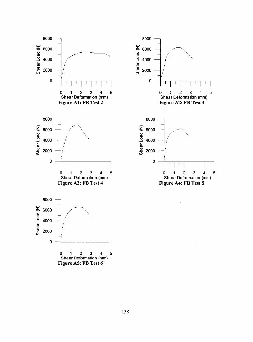
8000
-~ 6000 "0 (tJ
.3 4000 L. (tJ
~ 2000 Cf)
o
8000
-~ 6000 "0 (tJ
.3 4000 L. (tJ
~ 2000 Cf)
o
8000
-~ 6000 "0 (tJ
.3 4000 L. (tJ
~ 2000 Cf)
o
1 1 1 1 1 1 1 1 1 1
o 1 234 5 Shear Deformation (mm)
Figure Al: FB Test 2
1 1 1 1 1 1 1 1 1 1 1
o 1 234 5 Shear Deformation (mm)
Figure A3: FB Test 4
1 1 1 1 1 1 1 1 1 1 1
o 1 234 5 Shear Deformation (mm)
Figure AS: FB Test 6
138
8000
~ 6000 "0 (tJ
.3 4000 L. (tJ
~ 2000 Cf)
o
8000
-~ 6000 "0 (tJ
.3 4000 L. (tJ
~ 2000 Cf)
o
1 1 1 1 1 1 1 1 1 1
o 1 234 5 Shear Deformation (mm) Figure A2: FB Test 3
1 1 1 1 1 1 1 1 1 1 1
o 1 234 5 Shear Deformation (mm)
Figure A4: FB Test S
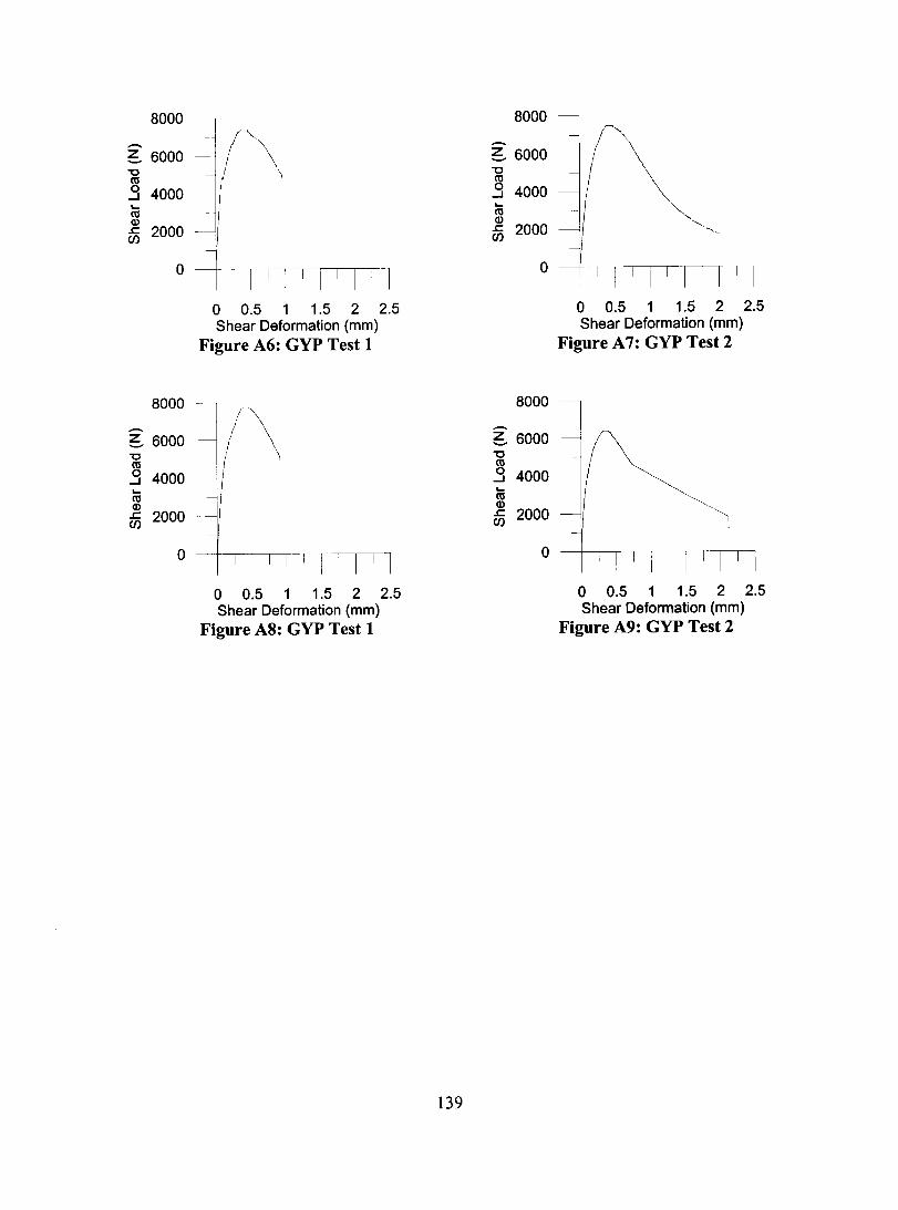
8000
-~ 6000 "0 CIl
..9 4000 ... CIl Q)
fA 2000
o
8000
-~ 6000 "0 CIl
..9 4000 ... CIl Q)
(\
1 1 1 1 1 r 1 1 1 1
o 0.5 1 1.5 2 2.5 Shear Deformation (mm)
Figure A6: GYP Test 1
fA 2000 -
o
o 0.5 1 1.5 2 2.5 Shear Deformation (mm)
Figure A8: GYP Test 1
139
8000
-~ 6000 "0 CIl
..9 4000 ... CIl Q)
fA 2000
o
8000
-~ 6000 "0 CIl
..9 4000 ... CIl Q)
fA 2000
o
o 0.5 1 1.5 2 2.5 Shear Deformation (mm)
Figure A7: GYP Test 2
o 0.5 1 1.5 2 2.5 Shear Deformation (mm)
Figure A9: GYP Test 2

APPENDIXB
FLEXURAL TEST DATA
The results of the flexural tests are presented in Chapter 3, Section 3.3 and in this
Appendix. The maximum loads as weIl as the thickness measurements of each specimen
are presented in this Appendix. Furthermore, the load versus displacement curve of each
specimen is also shown.
140
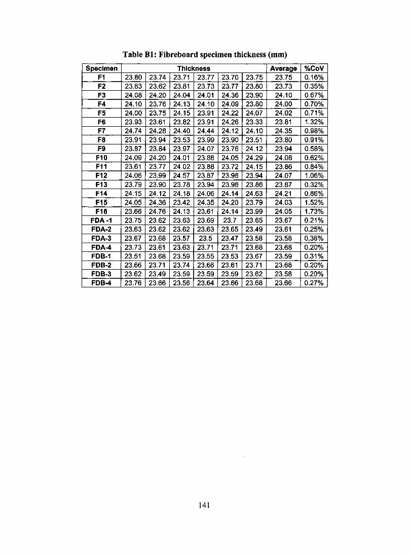
Table B1: Fibreboard specimen thickness (mm)
Specimen Thickness Average %CoV F1 23.80 23.74 23.71 23.77 23.70 23.75 23.75 0.16% F2 23.63 23.62 23.81 23.73 23.77 23.80 23.73 0.35% F3 24.08 24.20 24.04 24.01 24.36 23.90 24.10 0.67% F4 24.10 23.76 24.13 24.10 24.09 23.80 24.00 0.70% F5 24.00 23.75 24.15 23.91 24.22 24.07 24.02 0.71% F6 23.93 23.61 23.82 23.91 24.26 23.33 23.81 1.32% F7 24.74 24.28 24.40 24.44 24.12 24.10 24.35 0.98% F8 23.91 23.94 23.53 23.99 23.90 23.51 23.80 0.91% F9 23.87 23.84 23.97 24.07 23.76 24.12 23.94 0.58% F10 24.09 24.20 24.01 23.86 24.05 24.29 24.08 0.62% F11 23.61 23.77 24.02 23.88 23.72 24.15 23.86 0.84% F12 24.06 23.99 24.57 23.87 23.96 23.94 24.07 1.06% F13 23.79 23.90 23.78 23.94 23.96 23.86 23.87 0.32% F14 24.15 24.12 24.18 24.06 24.14 24.63 24.21 0.86% F15 24.05 24.36 23.42 24.35 24.20 23.79 24.03 1.52% F16 23.66 24.76 24.13 23.61 24.14 23.99 24.05 1.73%
FDA-1 23.75 23.62 23.63 23.69 23.7 23.65 23.67 0.21% FDA-2 23.63 23.62 23.62 23.63 23.65 23.49 23.61 0.25% FDA-3 23.67 23.68 23.57 23.5 23.47 23.58 23.58 0.36% FDA-4 23.73 23.61 23.63 23.71 23.71 23.68 23.68 0.20% FDB-1 23.51 23.68 23.59 23.55 23.53 23.67 23.59 0.31% FDB-2 23.66 23.71 23.74 23.66 23.61 23.71 23.68 0.20% FDB-3 23.62 23.49 23.59 23.59 23.59 23.62 23.58 0.20% FDB-4 23.76 23.66 23.56 23.64 23.66 23.68 23.66 0.27%
141
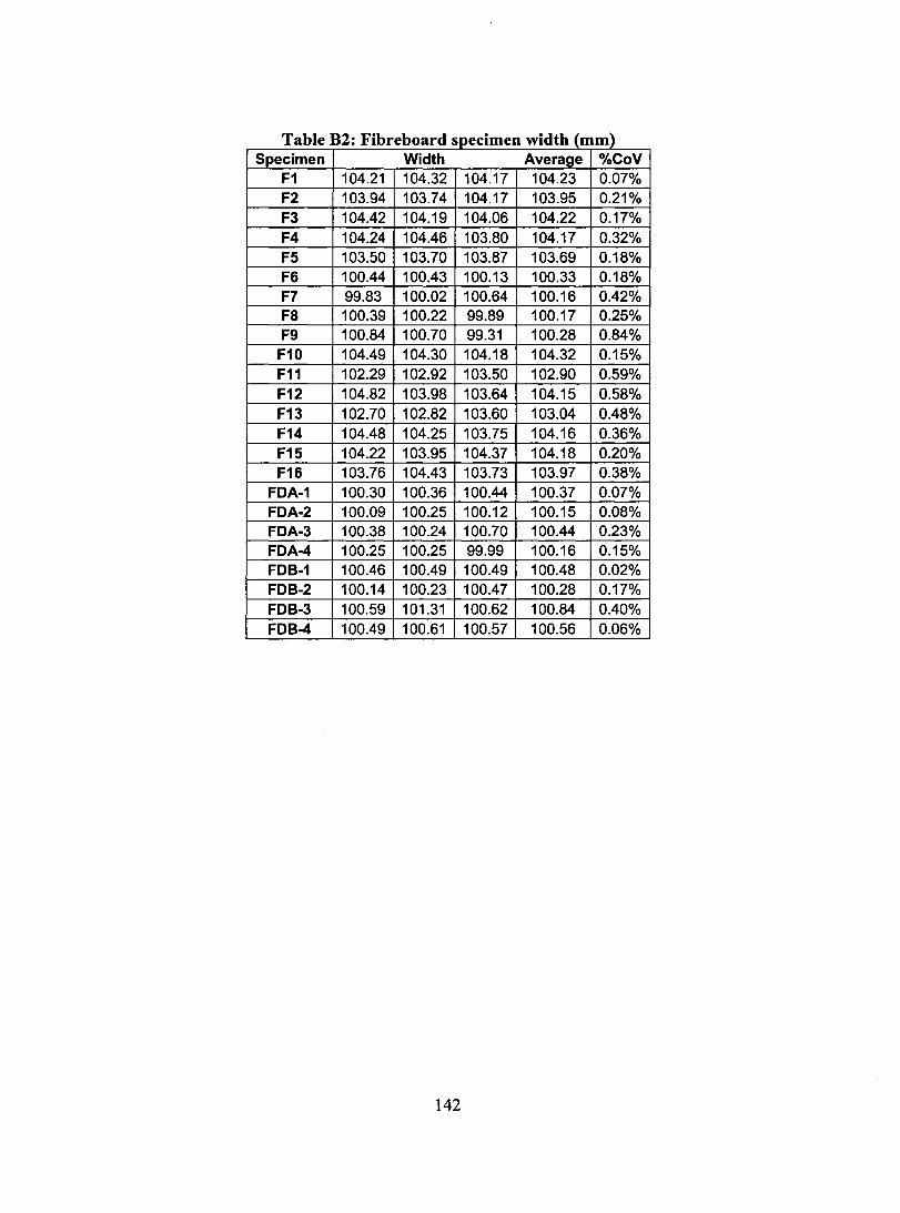
Table B2: Fibreboard specimen width (mm) Specimen Width Average %CoV
F1 104.21 104.32 104.17 104.23 0.07% F2 103.94 103.74 104.17 103.95 0.21% F3 104.42 104.19 104.06 104.22 0.17% F4 104.24 104.46 103.80 104.17 0.32% F5 103.50 103.70 103.87 103.69 0.18% F6 100.44 100.43 100.13 100.33 0.18% F7 99.83 100.02 100.64 100.16 0.42% F8 100.39 100.22 99.89 100.17 0.25% F9 100.84 100.70 99.31 100.28 0.84% F10 104.49 104.30 104.18 104.32 0.15% F11 102.29 102.92 103.50 102.90 0.59% F12 104.82 103.98 103.64 104.15 0.58% F13 102.70 102.82 103.60 103.04 0.48% F14 104.48 104.25 103.75 104.16 0.36% F15 104.22 103.95 104.37 104.18 0.20% F16 103.76 104.43 103.73 103.97 0.38%
FDA-1 100.30 100.36 100.44 100.37 0.07% FDA-2 100.09 100.25 100.12 100.15 0.08% FDA-3 100.38 100.24 100.70 100.44 0.23% FDA-4 100.25 100.25 99.99 100.16 0.15% FDB-1 100.46 100.49 100.49 100.48 0.02% FDB-2 100.14 100.23 100.47 100.28 0.17% FDB-3 100.59 101.31 100.62 100.84 0.40% FDB-4 100.49 100.61 100.57 100.56 0.06%
142

Table B3: Gypsum board specimen thickness (mm) Specimen Thickness Average %CoV
G-PL1 15.61 15.61 15.64 14.93 14.97 15.01 15.30 2.33% G-PL2 15.59 15.61 15.65 15.58 15.61 15.57 15.60 0.18% G-PL3 15.53 15.49 15.51 15.59 15.56 15.54 15.54 0.23% G-PL4 15.40 15.39 15.40 15.61 15.65 15.59 15.51 0.79% G-PL5 15.57 15.44 15.37 15.58 15.51 15.30 15.46 0.73% G-PL6 15.25 15.40 15.49 15.53 15.26 15.30 15.37 0.78% G-PL7 15.30 15.23 15.25 15.20 15.23 15.22 15.24 0.23% G-PL8 15.52 15.25 15.26 15.21 15.24 15.41 15.32 0.80% G-PL9 15.31 15.21 15.35 15.27 15.17 15.23 15.26 0.44%
G-PL10 15.68 15.51 15.60 15.60 15.36 15.34 15.52 0.89% G-PL11 15.63 15.65 15.68 15.59 15.61 15.57 15.62 0.26% G-PL 12 15.85 15.67 15.32 15.21 15.92 15.77 15.62 1.87% G-PL 13 15.52 15.52 15.51 15.55 15.53 15.50 15.52 0.11% G-PL14 15.52 15.52 15.51 15.45 15.45 15.44 15.48 0.25% G-PL 15 15.31 15.41 15.37 15.34 15.33 15.31 15.35 0.25% G-PL 16 15.32 15.32 15.29 15.22 15.22 15.22 15.27 0.33% G-PL 17 15.24 15.24 15.26 15.19 15.20 15.23 15.23 0.17% G-PL 18 15.25 15.22 15.22 15.19 15.23 15.23 15.22 0.13% G-PL 19 15.25 15.24 15.19 15.10 15.11 15.14 15.17 0.43% G-PL20 15.43 15.44 15.42 15.57 15.60 15.58 15.51 0.55% G-PL21 15.29 15.10 15.12 15.32 15.36 15.33 15.25 0.74% G-PL22 15.60 15.66 15.67 14.68 14.60 14.50 15.12 3.83% G-PP1 15.58 15.65 15.77 15.61 15.59 15.62 15.64 0.45% G-PP2 15.58 15.59 15.57 15.51 15.57 15.53 15.56 0.20% G-PP3 15.49 15.50 15.57 15.51 15.57 15.45 15.52 0.30% G-PP4 15.49 15.52 15.50 15.47 15.57 15.60 15.53 0.32% G-PP5 15.52 15.39 15.47 15.50 15.49 15.39 15.46 0.36% G-PP6 15.49 15.51 15.39 15.48 15.45 15.35 15.45 0.40% G-PP7 15.18 15.19 15.19 15.20 15.14 15.14 15.17 0.18% G-PP8 15.17 15.20 15.15 15.16 15.14 15.19 15.17 0.15% G-PP9 15.20 15.46 15.17 15.26 15.20 15.19 15.25 0.71%
G-PP10 15.17 15.17 15.18 15.19 15.19 15.12 15.17 0.17% G-PP11 15.14 15.15 15.16 15.17 15.14 15.11 15.15 0.14% G-PP12 15.85 15.67 15.32 15.21 15.92 15.77 15.62 1.87% G-PP13 15.52 15.52 15.51 15.55 15.53 15.50 15.52 0.11% G-PP14 15.52 15.52 15.51 15.45 15.45 15.44 15.48 0.25% G-PP15 15.31 15.41 15.37 15.34 15.33 15.31 15.35 0.25% G-PP16 15.32 15.32 15.29 15.22 15.22 15.22 15.27 0.33% G-PP17 15.24 15.24 15.26 15.19 15.20 15.23 15.23 0.17% G-PP18 15.25 15.22 15.22 15.19 15.23 15.23 15.22 0.13%
G-PP19 15.25 15.24 15.19 15.10 15.11 15.14 15.17 0.43% G-PP20 15.43 15.44 15.42 15.57 15.60 15.58 15.51 0.55% G-PP21 15.29 15.10 15.12 15.32 15.36 15.33 15.25 0.74% G-PP22 15.60 15.66 15.67 14.68 14.60 14.50 15.12 3.83%
143

Table B4: Gypsum board specimen width mm) Specimen Width Average %CoV
G-PL1 103.43 102.97 103.31 103.24 0.23% G-PL2 104.21 104.35 103.99 104.18 0.17% G-PL3 101.75 101.04 101.16 101.32 0.38% G-PL4 101.00 101.58 101.45 101.34 0.30% G-PL5 101.90 102.25 103.30 102.48 0.71% G-PL6 102.35 102.03 101.38 101.92 0.48% G-PL7 101.58 101.05 101.57 101.40 0.30% G-PL8 100.88 101.36 101.46 101.23 0.31% G-PL9 101.75 101.70 102.52 101.99 0.45%
G-PL10 102.07 102.74 103.03 102.61 0.48% G-PL11 102.66 102.64 103.03 102.78 0.21% G-PL12 103.73 104.02 103.21 103.65 0.40% G-PL13 103.95 103.75 104.10 103.93 0.17% G-PL 14 103.78 103.90 103.86 103.85 0.06% G-PL15 104.10 104.30 104.23 104.21 0.10% G-PL 16 104.12 103.88 104.16 104.05 0.15% G-PL17 104.18 103.95 104.20 104.11 0.13% G-PL 18 104.30 103.98 104.21 104.16 0.16% G-PL19 104.43 104.14 104.03 104.20 0.20% G-PL20 103.82 104.43 104.61 104.29 0.40% G-PL21 103.85 104.40 103.96 104.07 0.28% G-PL22 104.29 104.27 104.42 104.33 0.08% G-PP1 100.70 100.82 101.11 100.88 0.21% G-PP2 102.10 102.00 102.15 102.08 0.07% G-PP3 102.94 102.53 102.95 102.81 0.23% G-PP4 100.92 101.14 100.97 101.01 0.11% G-PP5 101.09 101.42 102.22 101.58 0.57% G-PP6 102.60 102.70 103.31 102.87 0.37% G-PP7 101.72 101.72 102.09 101.84 0.21% G-PP8 101.03 101.98 101.05 101.35 0.54% G-PP9 102.30 102.80 103.16 102.75 0.42%
G-PP10 101.91 101.91 101.95 101.92 0.02% G-PP11 101.07 101.08 101.14 101.10 0.04% G-PP12 104.31 104.54 104.42 104.42 0.11% G-PP13 102.75 102.83 103.85 103.14 0.59% G-PP14 104.11 103.86 103.79 103.92 0.16% G-PP15 103.60 103.90 103.58 103.69 0.17% G-PP16 104.15 103.85 103.75 103.92 0.20% G-PP17 103.12 103.58 103.76 103.49 0.32% G-PP18 104.24 104.30 104.19 104.24 0.05% G-PP19 103.99 103.96 103.81 103.92 0.09% G-PP20 103.85 103.77 103.82 103.81 0.04% G-PP21 103.75 103.79 103.89 103.81 0.07% G-PP22 104.20 104.63 104.25 104.36 0.23%
144

Table B5: FOb b d 1 re oar If ate load (N) specimen U lm Specimen Ultimate Load
F1 235.66 F2 229.4 F3 223.23 F4 215.1 F5 225.26 F6 211.18 F7 219.16 Fa 207.04 F9 206.96 F10 227.67 F11 233.62 F12 204.93 F13 220.82 F14 218.03 F15 243.49 F16 220.82
FDA-1 235.66
FDA-2 222.7
FDA-3 216.6 FDA-4 222.4 FDB-1 175.63 FDB-2 190.02 FDB-3 208.09 FDB-4 207.11
145
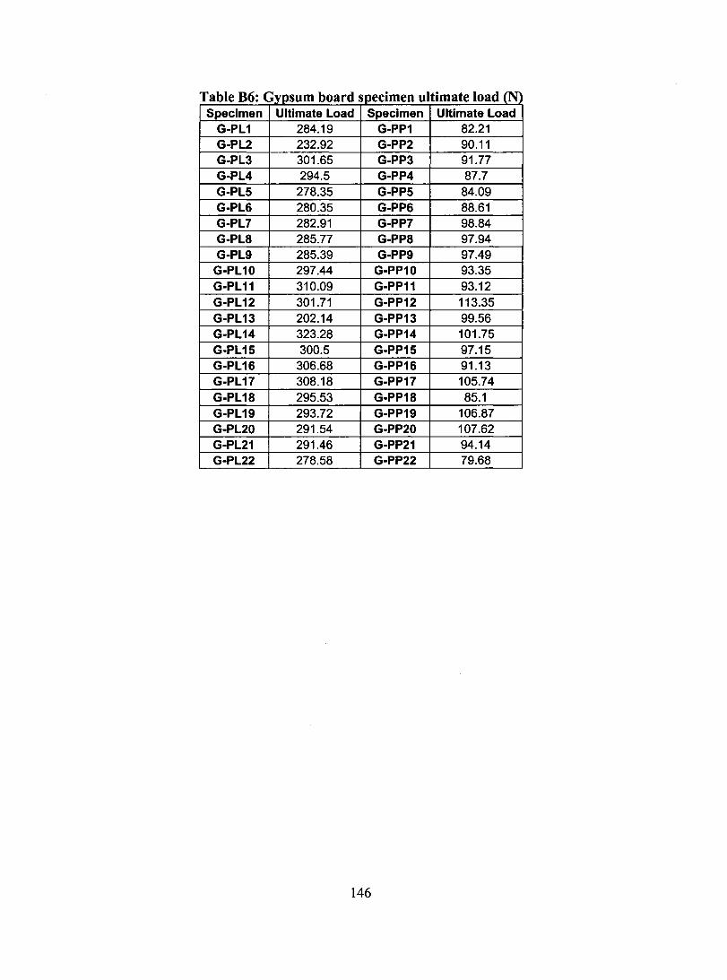
Table B6: Gypsum board specimen ultimate load (N) Specimen Ultimate Load Specimen Ultimate Load
G-PL1 284.19 G-PP1 82.21 G-PL2 232.92 G-PP2 90.11 G-PL3 301.65 G-PP3 91.77 G-PL4 294.5 G-PP4 87.7 G-PL5 278.35 G-PP5 84.09 G-PL6 280.35 G-PP6 88.61 G-PL7 282.91 G-PP7 98.84 G-PL8 285.77 G-PP8 97.94 G-PL9 285.39 G-PP9 97.49
G-PL10 297.44 G-PP10 93.35 G-PL11 310.09 G-PP11 93.12 G-PL12 301.71 G-PP12 113.35 G-PL13 202.14 G-PP13 99.56 G-PL14 323.28 G-PP14 101.75 G-PL15 300.5 G-PP15 97.15 G-PL16 306.68 G-PP16 91.13 G-PL17 308.18 G-PP17 105.74 G-PL18 295.53 G-PP18 85.1 G-PL19 293.72 G-PP19 106.87 G-PL20 291.54 G-PP20 107.62 G-PL21 291.46 G-PP21 94.14 G-PL22 278.58 G-PP22 79.68
146

..-..
250
200
~ 150 "t:I
~ 100 ....J
..-..
50
o
250
200
~ 150 "t:I
~ 100 ....J
..-..
50
o
250
200
~ 150 "t:I
~ 100 ....J
..-..
50
o
250
200
~ 150 "t:I
~ 100 ....J
50
o
o 4 8 12 16 20 Displacement (mm)
Figure BI: FBl
o 4 8 12 16 20 Displacement (mm)
Figure B3: FB3
o 4 8 12 16 20 Displacement (mm)
Figure B5: FB5
o 4 8 12 16 20 Displacement (mm)
Figure B7: FB7
147
..-..
250
200
~ 150 "t:I
~ 100 ....J
50
o
..-..
250
200
~ 150 "t:I
~ 100 ....J
..-..
50
o
250
200
~ 150 "t:I
~ 100 ....J
..-..
50
o
250
200
~ 150 "t:I
~ 100 ....J
50
o
o 4 8 12 16 20 Displacement (mm)
Figure B2: FB2
o 4 8 12 16 20 Displacement (mm) Figure B4: FB4
o 4 8 12 16 20 Displacement (mm) Figure B6: FB6
o 4 8 12 16 20 Displacement (mm) Figure B8: FB8
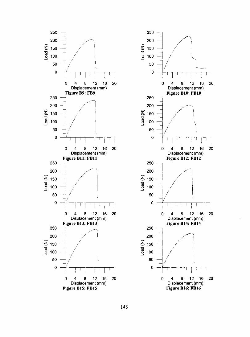
-250
200
~ 150 "t:l
~ 100 ..J
-
50
o
250
200
~ 150 "t:l
~ 100 ..J
-
50
o
250
200
~ 150 "t:l
~ 100 ..J
-
50
o
250
200
~ 150 "t:l
~ 100 ...J
50
o
1 1 1 1
o 4 8 12 16 20 Displacement (mm)
Figure B9: FB9
o 4 8 12 16 20 Displacement (mm)
Figure B11: FB11
o 4 8 12 16 20 Displacement (mm)
Figure B13: FB13
o 4 8 12 16 20 Displacement (mm)
Figure BIS: FB15
148
-250
200
~ 150 "t:l
~ 100 ..J
50
o --~~~~~~~~-
-250
200
~ 150 "t:l
~ 100 ..J
50
o
250
200
~ 150 "t:l
~ 100 ...J
50
o 4 8 12 16 20 Displacement (mm)
Figure BIO: FBI0
o 4 8 12 16 20 Displacement (mm)
Figure B12: FB12
o --~~~~~~~~-
-250
200
~ 150 "t:l
~ 100 ...J
50
o
o 4 8 12 16 20 Displacement (mm)
Figure B14: FB14
o 4 8 12 16 20 Displacement (mm)
Figure B16: FB16

250 250
200 200 - -~ 150 ~ 150 "0 "0 cu 100 cu 100 0 0
..J ..J
50 50
0 0
0 4 8 12 16 0 4 8 12 16 Displacement (mm) Displacement (mm)
Figure B17: FDA-l Figure B18: FDA-2 250 250
200 200 - -~ 150 ~ 150 "0 "0 cu 100 cu 100 0 0 ..J ..J
50 50
0 0
0 4 8 12 16 0 4 8 12 16 Displacement (mm) Displacement (mm)
Figure B19: FDA-3 Figure B20: FDA-4 250 250
200 200 - -~ 150 ~ 150 "0 "0 cu 100 cu 100 0 0
..J ..J
50 50
0 0
0 4 8 12 16 0 4 8 12 16 Displacement (mm) Displacement (mm)
Figure B21: FDB-l Figure B22: FDB-2 250 250
200 200 - -~ 150 ~ 150 "0 "0 cu 100 cu 100 0 0
...J ...J
50 50
0 0
0 4 8 12 16 0 4 8 12 16 Displacement (mm) Displacement (mm)
Figure B23: FDB-3 Figure B24: FDB-4
149
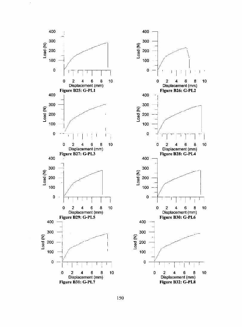
400 400
300 300 ..-. ..-. b z -"0 200 "0 200 co co a a ...J ...J
100 100
0 0
0 2 4 6 8 10 0 2 4 6 8 10 Displacement (mm) Displacement (mm)
Figure B25: G-PLI Figure B26: G-PL2 400 400
300 300 ..-. ..-. b b "0 200 "0 200 co co a a ...J ...J
100 100
0 T Tl- T TiT-r-1 0 1
1
1
1
1
1
1 Il
0 2 4 6 8 10 0 2 4 6 8 10 Displacement (mm) Displacement (mm)
Figure B27: G-PL3 Figure B28: G-PL4 400 400
300 300 ..-. ..-. b z -"0 200 "0 200 co co a a ...J ...J
100 100
0 - 0
0 2 4 6 8 10 0 2 4 6 8 10 Displacement (mm) Displacement (mm)
Figure B29: G-PL5 Figure B30: G-PL6 400 400
300 300 ..-. ..-. z b -"0 200 "0 200 co co 0 a
...J ...J
100 100
0 0
0 2 4 6 8 10 0 2 4 6 8 10 Displacement (mm) Displacement (mm)
Figure B31: G-PL7 Figure B32: G-PL8
150

400
300 -~ "0 200 CIl o -1
100
o
400
300 -~ -g 200 o -1
100
o
400
1 1 1 1 1 1 1
o 2 4 6 8 10 Displacement (mm)
Figure B33: G-PL9
--TT~rl
o 2 4 6 8 10 Displacement (mm)
Figure B35: G-PLll
300 ---~ -g 200 o -1
-z -
100
o
400
300
"0 200 CIl o
...J
100
o
o 2 4 6 8 10 Displacement (mm)
Figure B37: G-PL13
Till l--rrl o 2 4 6 8 10
Displacement (mm) Figure B39: G-PL15
151
400
300 z --g 200 o -1
~
100
o
400
300
-g 200 o -1
-~
100
o
400
300
-g 200 o -1
z -
100
o
400
300
-g 200 o
...J
100
o
o 2 4 6 8 10 Displacement (mm)
Figure B34: G-PLIO
o 2 4 6 8 10 Displacement (mm)
Figure B36: G-PL12
o 2 4 6 8 10 Displacement (mm)
Figure B38: G-PL14
o 2 4 6 8 10 Displacement (mm)
Figure B40: G-PL16
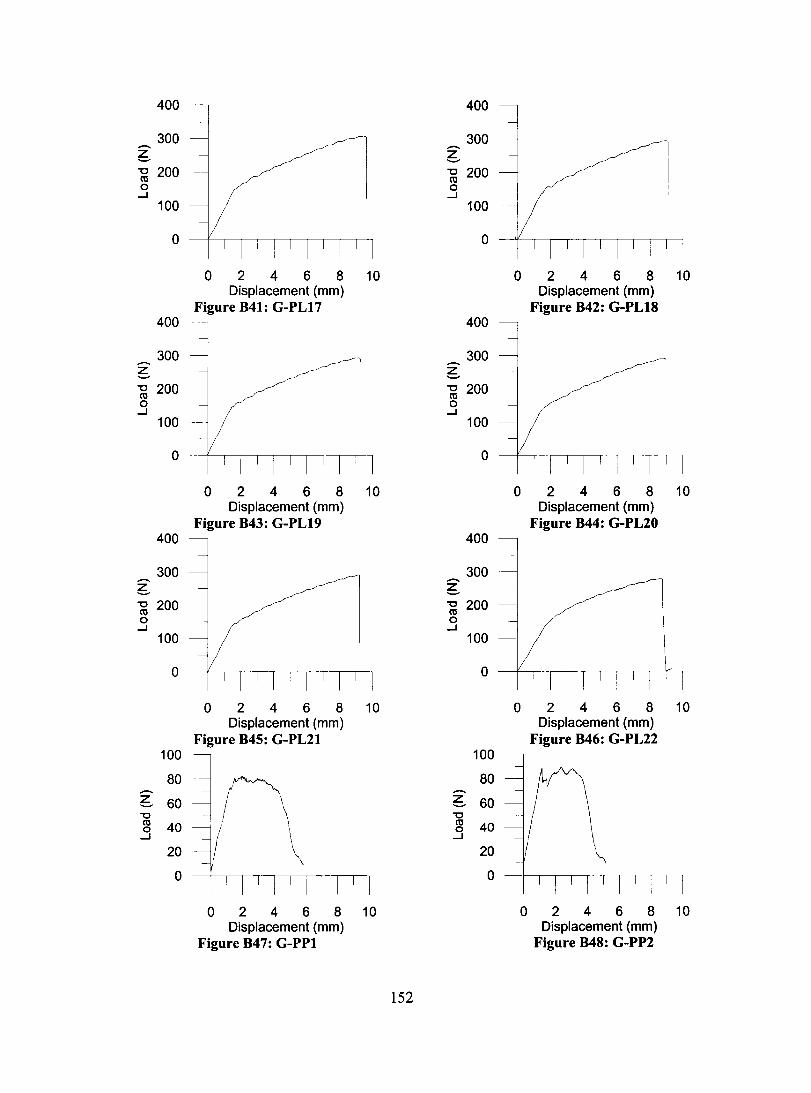
400
300 ~ "0 200 «l o
....J
100
o
400
300 z -"0 200 «l o
....J 100
o
400
300
"0 200 «l o
....J
-
100
o
100
80
~ 60 "0
~ 40 ....J
20
o
o 2 4 6 8 10 Displacement (mm)
Figure B41: G-PLI7
1 1 1 I~l o 2 4 6 8 10
Displacement (mm) Figure B43: G-PLI9
o 2 4 6 8 10 Displacement (mm)
Figure B45: G-PL21
o 2 4 6 8 10 Displacement (mm)
Figure B47: G-PPI
152
400
300 ~ "0 200 «l o
....J
100
o
400
300 -z -"0 200 «l o
....J 100
o
400
300
"0 200 «l o
....J
-
100
o
100
80
~ 60 "0
~ 40 ....J
20
o
o 2 4 6 8 10 Displacement (mm)
Figure B42: G-PLI8
1 1 1 'T'TIl o 2 4 6 8 10
Displacement (mm) Figure B44: G-PL20
o 2 4 6 8 10 Displacement (mm)
Figure B46: G-PL22
o 2 4 6 8 10 Displacement (mm)
Figure B48: G-PP2
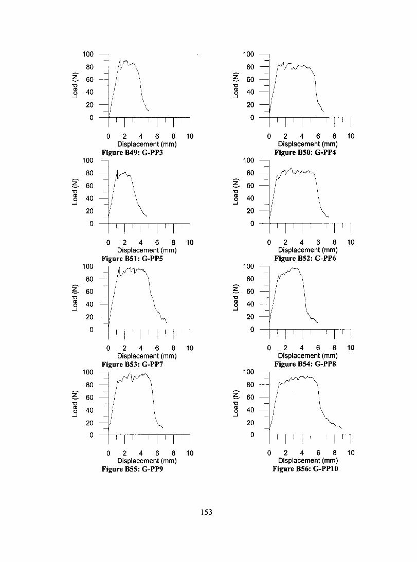
100 100
80 - 80 - -
\ z 60 z 60 - -"0 "0 (Il 40 (Il 40 0 0
....J ....J
20 20
0 0
0 2 4 6 8 10 0 2 4 6 8 10 Displacement (mm) Displacement (mm)
Figure B49: G-PP3 Figure B50: G-PP4 100 -~ 100
80 80 - -z 60 z 60 - -"0 "0 (Il 40 (Il 40 0 0
....J ....J
20 20
0 1
1
1
1
1
1
1
1
0
0 2 4 6 8 10 0 2 4 6 8 10 Displacement (mm) Displacement (mm)
Figure B51: G-PP5 Figure B52: G-PP6 100 100
80 80 - -~ 60 ~ 60 "0 "0 (Il 40 (Il 40 0 0
....J ....J
20 20
0 0
0 2 4 6 8 10 0 2 4 6 8 10 Displacement (mm) Displacement (mm)
Figure B53: G-PP7 Figure B54: G-PP8 100 100
80 80 - -z 60 ~ 60 -"0 "0 (Il 40 (Il 40 0 0
....J ....J
20 20
0 0
0 2 4 6 8 10 0 2 4 6 8 10 Displacement (mm) Displacement (mm)
Figure B55: G-PP9 Figure B56: G-PPI0
153
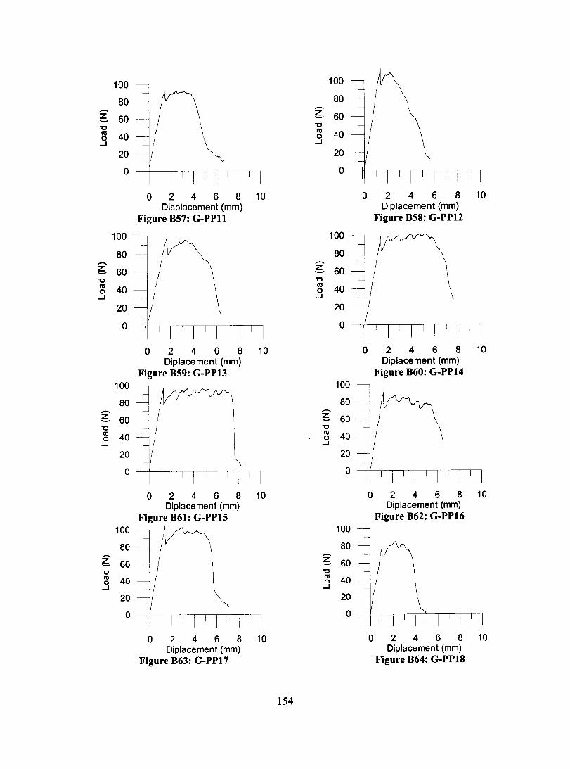
100 100
80 80 -z 60 '-' 6 60
"0 "0 ro 40
ro 40 0 0 ...J ...J
20 20
0 1
1
1
1
1
1
1 0 -l
0 2 4 6 8 10 0 2 4 6 8 10 Displacement (mm) Diplacement (mm)
Figure B57: G-PPll Figure B58: G-PP12
100 100
80 -- 80 - -6 60 6 60 "0 "0 ro 40 ro 40 0 0
...J ...J
20 20
0 0
0 2 4 6 8 10 0 2 4 6 8 10 Diplacement (mm) Diplacement (mm)
Figure B59: G-PP13 Figure B60: G-PPI4 100 100
80 80 - -~ 60 ~ 60 "0 "0 ro 40 ro 40 0 0
...J ...J
20 20
0 0
0 2 4 6 8 10 0 2 4 6 8 10 Diplacement (mm) Diplacement (mm)
Figure B61: G-PPI5 Figure B62: G-PPI6 100 100
80 80
~ -60 ~ 60 "0 "0 ro 40 ro 40 0 0
...J ...J
20 20
0 0
0 2 4 6 8 10 0 2 4 6 8 10 Diplacement (mm) Diplacement (mm)
Figure B63: G-PPI7 Figure B64: G-PPI8
154
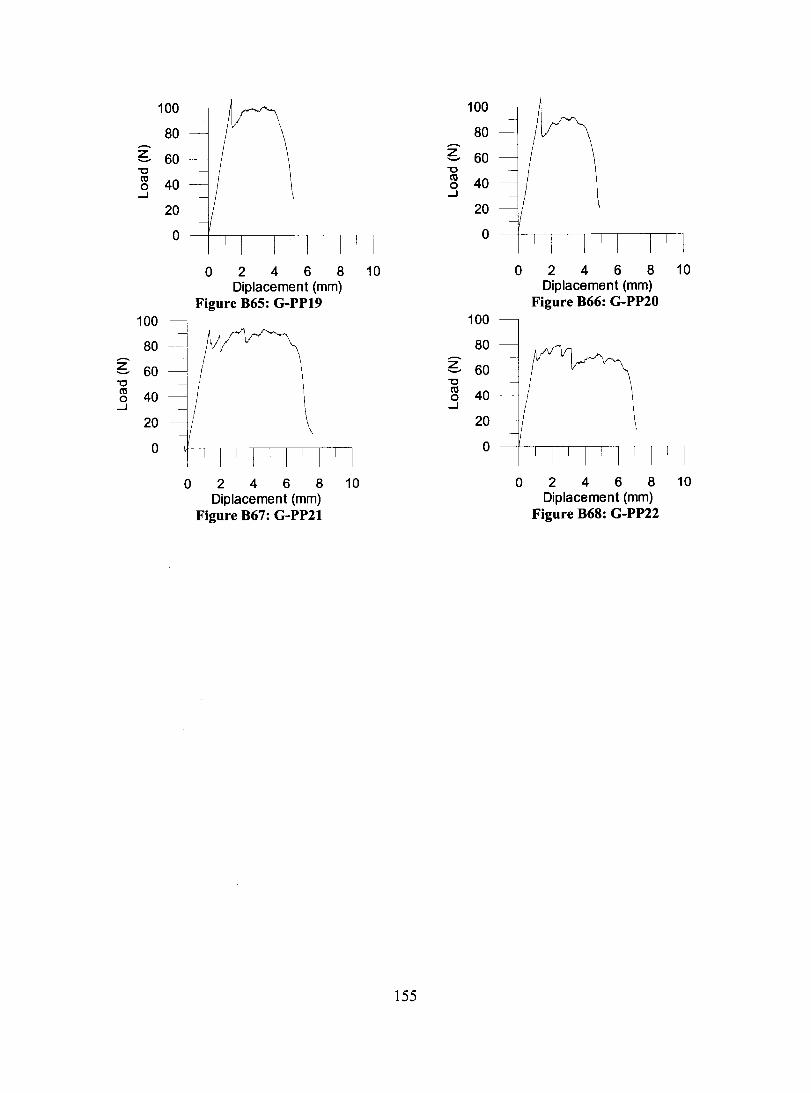
100 100
80 80 - -z 60 z 60 - -"0 "0 co 40 co 40 0 0 ...J ...J
20 20
0 0
0 2 4 6 8 10 0 2 4 6 8 10 Diplacement (mm) Diplacement (mm)
Figure B65: G-PP19 Figure B66: G-PP20 100 100
80 80 - Z ~ 60 - 60 "0 "0 co 40 co 40 0 0 ...J ...J
20 - 20
0 1
1
1
1
1
1
1
1
1
1
0
0 2 4 6 8 10 0 2 4 6 8 10 Diplacement (mm) Diplacement (mm)
Figure B67: G-PP21 Figure B68: G-PP22
155

APPENDIXC
FOUR-SIDED SHEAR TEST DATA
The results of the four-sided shear tests are presented in Chapter 3, Section 3.4 and in this
Appendix. The load versus elongation curve and a table summarizing the experimental
data acquired for each specimen in presented in this Appendix.
156

Table Cl: FBI data
FB1 Dimensions measured before testing Stiffness
Thickness at corners (mm) T1
1
T2
1
T3
1
T4 Siope 1 Siope 2 NIA NIA NIA NIA 18938 NIA
Average Thickness (mm) Average Siope 23.52
Length of Sides (in) L1
1
L2 24.25 24.31
Average Length (mm) 616.35
40000
30000
-z -'0 20000 ca o .....J
10000 -
o
-1
18938
1
L3
1
L4 Stiffness 24.25 24.25 234
Gauge Length (mm) 508
o 1 Elongation(mm)
Figure Cl: FBlload vs. elongation
157
MPa
2

Table C2: FB2 data FB2
Dimensions measured before testing Stiffness
Thickness at corners (mm) T1
1
T2
1
T3
1
T4 Siope 1 Siope 2 NIA NIA NIA NIA 19334 NIA
Average Thickness (mm) Average Siope 23.52
Length of Sides (in) L1
1
L2 24.13 24.13
Average Length (mm) 613.30
40000
30000
-z -""C 20000 -rn o ....J
10000
o
-1
19334
Stiffness
1 L3
1
L4 24.19 NIA 241
Gauge Length (mm) 508
o 1 Elongation(mm)
Figure C2: FB2load vs. elongation
158
MPa
2
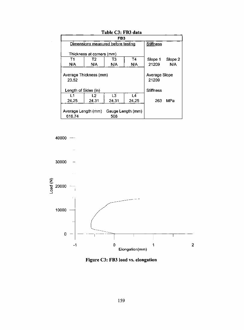
Table C3: FB3 data FB3
Dimensions measured before testing Stiffness
Thickness at corners (mm) T1
1
T2
1
T3
1
T4 Siope 1 Siope 2 NIA NIA NIA NIA 21209 NIA
Average Thickness (mm) Average Siope 23.52
Length of Sides (in) L1
1
L2 24.25 24.31
Average Length (mm) 616.74
40000
30000
-~ -g 20000 o
....J
10000
o
-1
21209
Stiffness
1
L3
1
L4 24.31 24.25 263
Gauge Length (mm) 508
o 1 Elongation(mm)
Figure C3: FB3 load vs. elongation
159
MPa
2
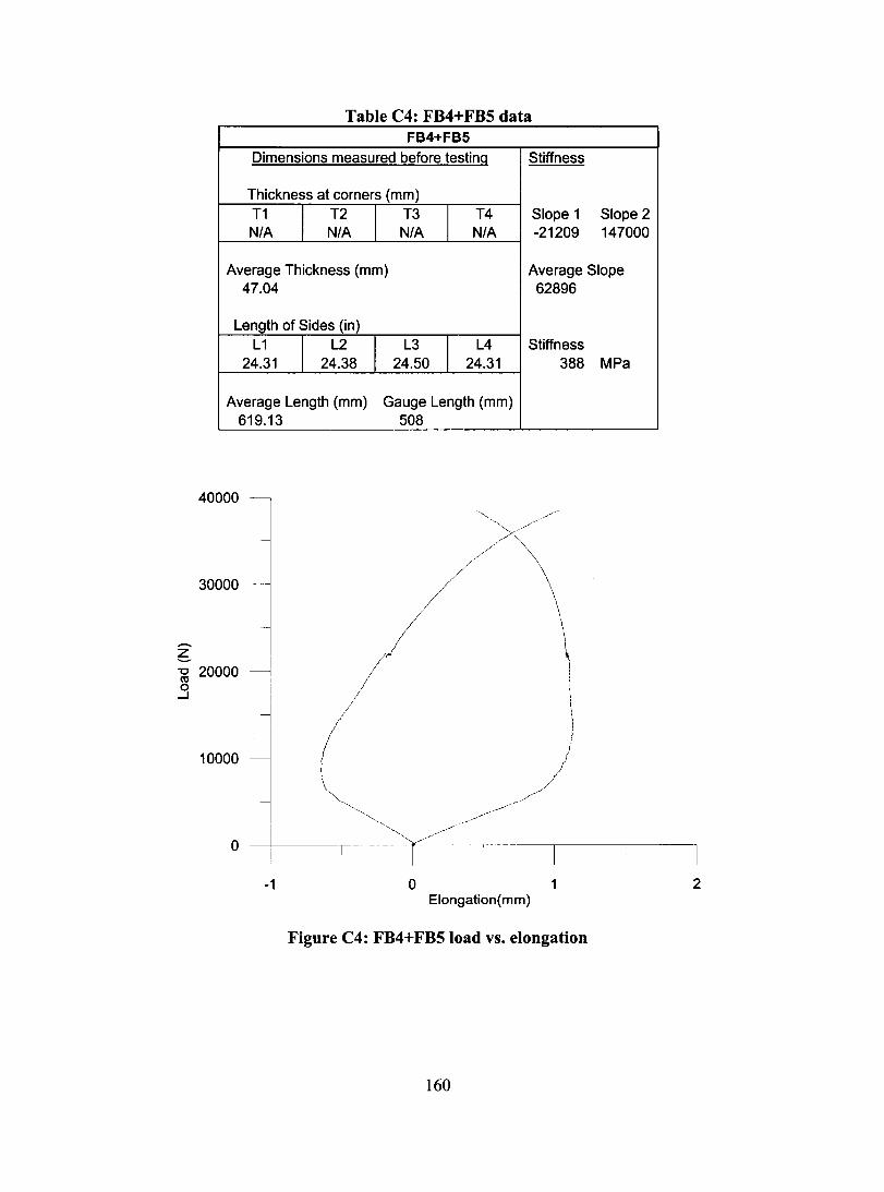
Table C4: FB4+FB5 data FB4+FB5
Dimensions measured before testing Stiffness
Thickness at corners (mm) T1
1
T2
1
T3
1
T4 Siope 1 Siope 2 NIA NIA NIA NIA -21209 147000
Average Thickness (mm) Average Siope 47.04
Length of Sides (in) L1
1
L2 24.31 24.38
Average Length (mm) 619.13
40000
30000
-~ ~ 20000 o
...J
10000
o
-1
62896
1
L3
1
L4 Stiffness 24.50 24.31 388
Gauge Length (mm) 508
o 1 Elongation(mm)
Figure C4: FB4+FB5Ioad vs. elongation
160
MPa
2
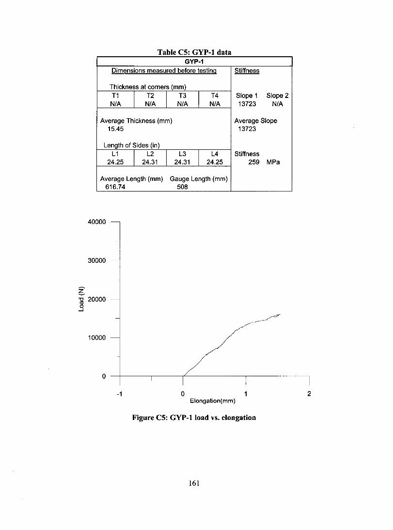
Table CS: GYP-l data GYP-1
Dimensions measured before testing Stiffness
Thickness at corners (mm) T1
1
T2
1
T3
1
T4 Siope 1 Siope 2 NIA NIA NIA NIA 13723 NIA
Average Thickness (mm) Average Siope 15.45
Length of Sides (in) L1
1
L2 24.25 24.31
Average Length (mm) 616.74
40000
30000
.-.. ~ ~ 20000 o
...J
10000
o
-1
13723
1
L3
1
L4 Stiffness 24.31 24.25 259
Gauge Length (mm) 508
o 1 Elongation(mm)
Figure CS: GYP-l load vs. elongation
161
MPa
2

Table C6: FB-2 STIFF data FB-2 STIFF
Dimensions measured before testing Stiffness
Thickness at corners (mm) T1
1
T2
1
T3
1
T4 Siope 1 Siope 2 23.26 23.06 23 22.88 19693 25743
Average Thickness (mm) Average Siope 23.05 22718
Length of Sides (in) L1
1 L2 1
L3
1
L4 Stiffness 24.25 24.3125 24.25 24.25 287 MPa
Average Length (mm) Gauge Length (mm) 616.34 508
30000
20000
...-~ "0 CIl 0
...J
10000
o
-1 o 1 2 Elongation (mm)
Figure C6: FB-2 STIFF load vs. elongation
162

-z -"0 CIl o
...J
Table C7: FB-3 STIFF data FB-3 STIFF
Dimensions measured before testing Stiffness
Thickness at corners (mm) T1
1
T2 1 T3
1
T4 Siope 1 Siope 2 23.26 23.10 23.14 23.1 13869 17431
Average Thickness (mm) Average Siope 23.15 15650
Length of Sides (in) L1
1
L2
1
L3
1
L4 Stiffness 24.13 24.13 24.19 NIA 198 MPa
Average Length (mm) Gauge Length (mm) 613.30 508
30000
20000
10000 ~
o
-1 o 1 2 Elongation (mm)
Figure C7: FB-3 STIFF load vs. elongation
163
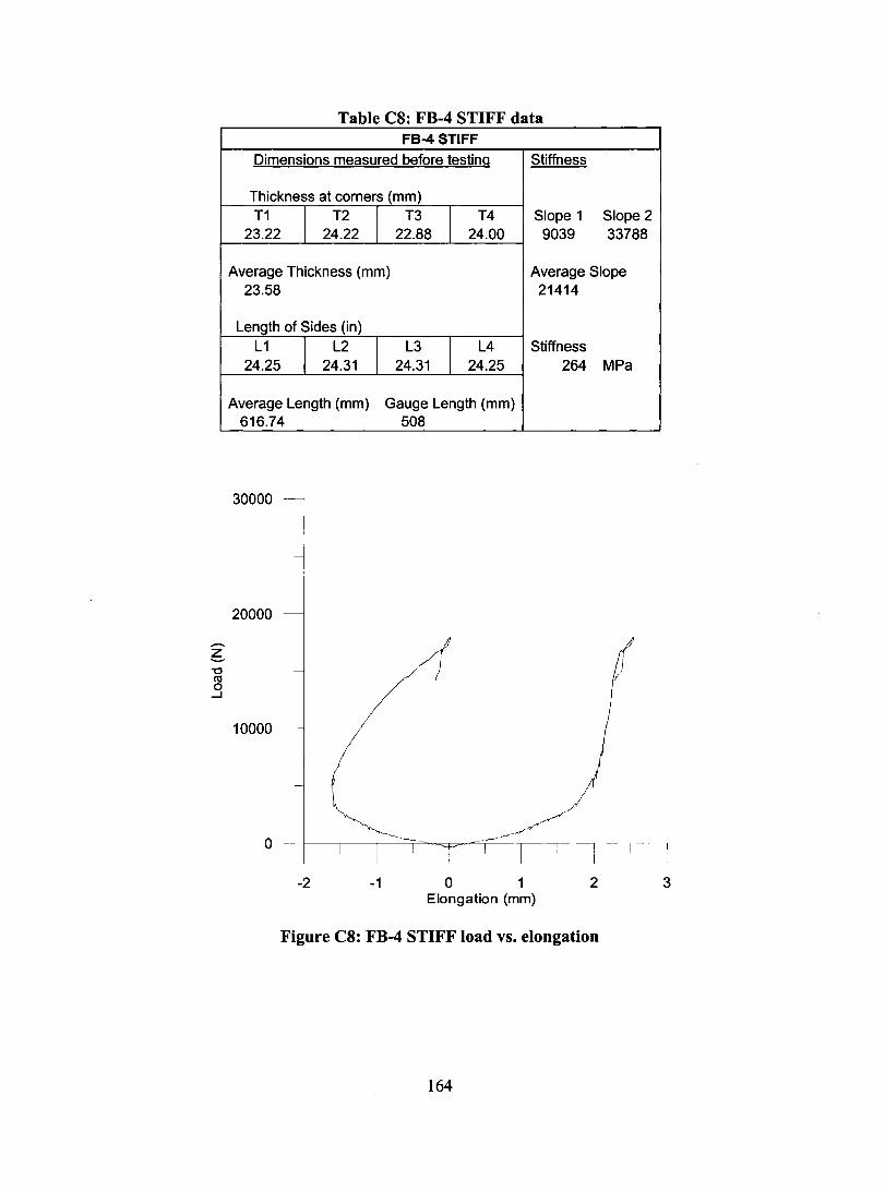
Table CS: FB-4 STIFF data FB-4 STIFF
Dimensions measured before testing Stiffness
Thickness at corners (mm) T1
1 T2 1
T3
1
T4 Siope 1 Siope 2 23.22 24.22 22.88 24.00 9039 33788
Average Thickness (mm) Average Siope 23.58 21414
Length of Sides (in) L1
_1
L2 1 L3
1
L4 Stiffness 24.25 24.31 24.31 24.25 264 MPa
Average Length (mm) Gauge Length (mm) 616.74 508
30000
20000
.-.. 6--0 «l 0
...J
10000
o
-2 -1 o 1 2 3 Elongation (mm)
Figure C8: FB-4 STIFF load vs. elongation
164
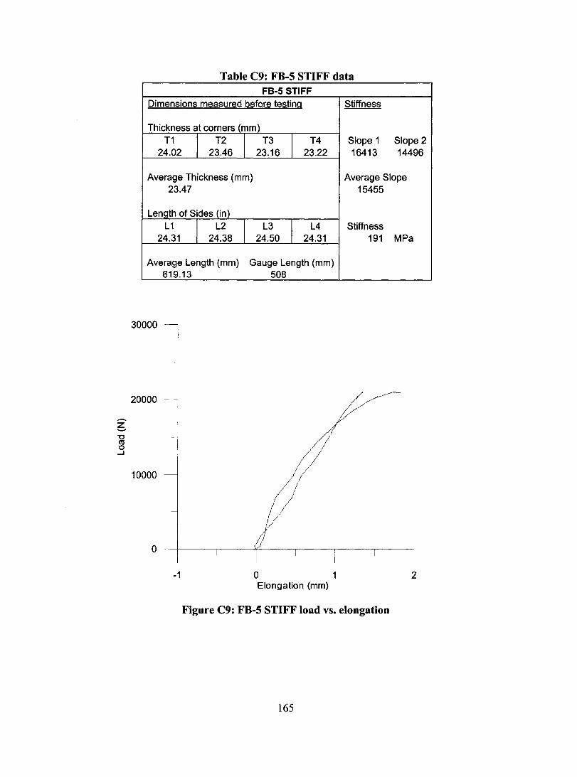
Table C9: FB-5 STIFF data FB-5 STIFF
Dimensions measured before testing Stiffness
Thickness at corners (mm) T1
1 T2 l T3
1
T4 Siope 1 Siope 2 24.02 23.46 23.16 23.22 16413 14496
Average Thickness (mm) Average Siope 23.47 15455
Length of Sides (in) L1
1
L2
1
L3
1
L4 Stiffness 24.31 24.38 24.50 24.31 191 MPa
Average Length (mm) Gauge Length (mm) 619.13 508
30000
20000
-z -'0 ro 0
.....J
10000
o
-1 o 1 2 Elongation (mm)
Figure C9: FB-5 STIFF load vs. elongation
165

Table CIO: GYP-I STIFF data GYP-1STIFF
Dimensions measured before testing Stiffness
Thickness at corners (mm) T1
1 T2 1
T3
1
T4 Siope 1 Siope 2 15.52 15.58 15.28 15.42 17456 12540
Average Thickness (mm) Average Siope 15.45 14998
Length of Sides (in) L1
1
L2
1
L3
1
L4 Stiffness 24.50 24.50 24.38 NIA 281 MPa
Average Length (mm) Gauge Length (mm) 621.24 508
25000
20000
15000 z .........
10000
5000
o
-1 o 1 2 Elongation (mm)
Figure CIO: GYP-I STIFF load vs. elongation
166

Table CU: GYP-2 STIFF data GYP-2 STIFF
Dimensions measured before testing Stiffness
Thickness at corners (mm) T1
1 T2 1 T3 1 T4 Slope 1 Slope 2 15.28 15.70 15.50 15.72 60304 91898
Average Thickness (mm) Average Slope 15.55 76101
Length of Sides (in) Stiffness L1
1 2;.;1 1
L3
1
L4 24.34 24.34 24.31 1423 MPa
Average Length Gauge Length (mm) (mm)
617.93 508
25000
20000
15000 ..-.. z -'0 CIl 0
....J 10000 -
5000
o
-1 o 1 2 Elongation (mm)
Figure CU: GYP-2 STIFF load vs. elongation
167

Table CI2: GYP-3 STIFF data GYP-3 STIFF
Dimensions measured before testing Stiffness
Thickness at corners (mm) T1
1
T2
1
T3
1
T4 Siope 1 Siope 2 15.40 15.56 15.46 15.50 16335 8081
Average Thickness (mm) Average Siope 15.48 12208
Length of Sides (in) L1
1
L2
1
L3
1
L4 Stiffness 24.38 24.38 24.38 24.38 229 MPa
Average Length (mm) Gauge Length (mm) 619.13 508
25000
20000 --
15000 ........ ~ "0 en 0
...J
10000
5000
o
-1 o 1 2 Elongation (mm)
Figure CI2: GYP-3 STIFF load vs. elongation
168
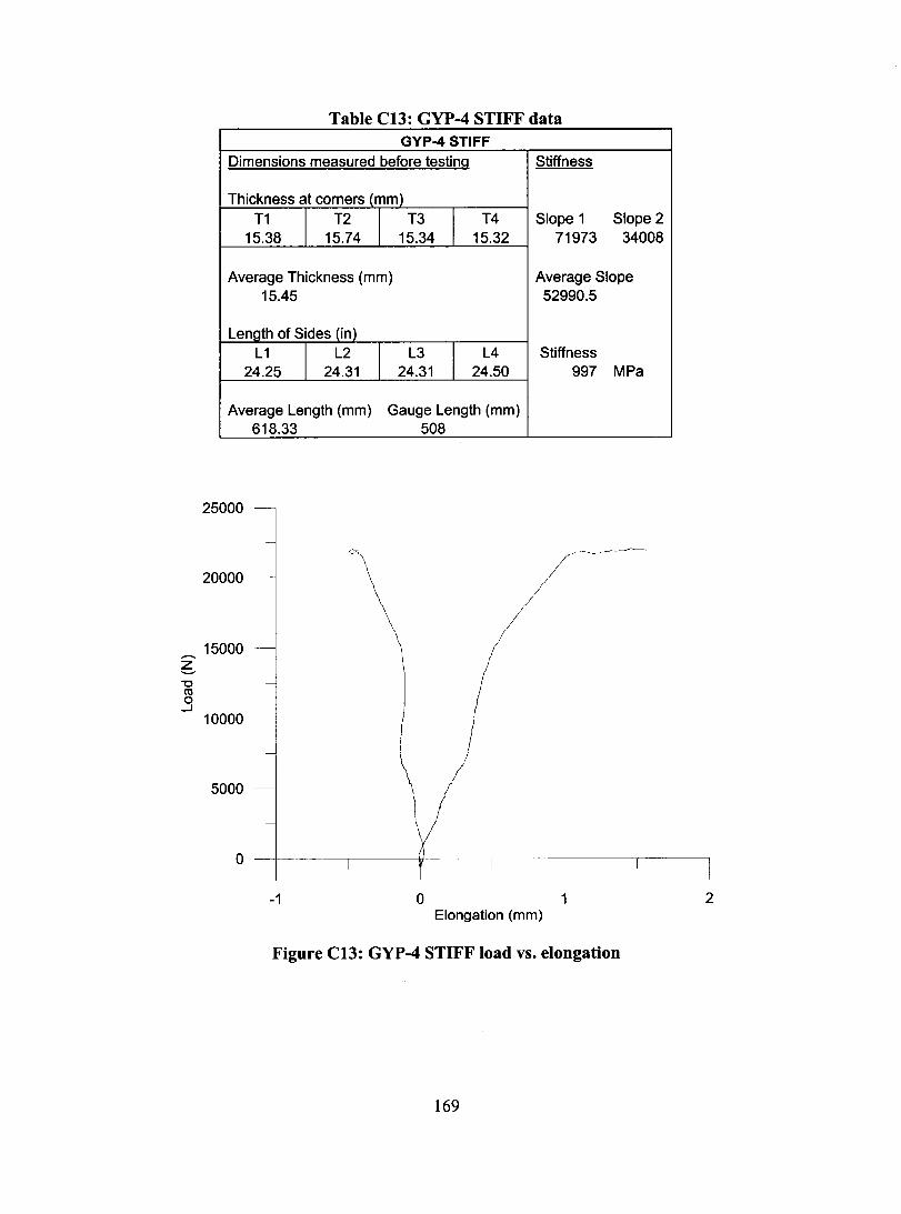
Table C13: GYP-4 STIFF data GYP-4STIFF
Dimensions measured before testing Stiffness
Thickness at corners (mm) T1
1
T2
1
T3
1
T4 Siope 1 Siope 2 15.38 15.74 15.34 15.32 71973 34008
Average Thickness (mm) Average Siope 15.45 52990.5
Length of Sides (in) L1
1 L2
1
L3 1
L4 Stiffness 24.25 24.31 24.31 24.50 997 MPa
Average Length (mm) Gauge Length (mm) 618.33 508
25000
20000
15000 z -
10000
5000
o
-1 o 1 2 Elongation (mm)
Figure C13: GYP-4 STIFF load vs. elongation
169
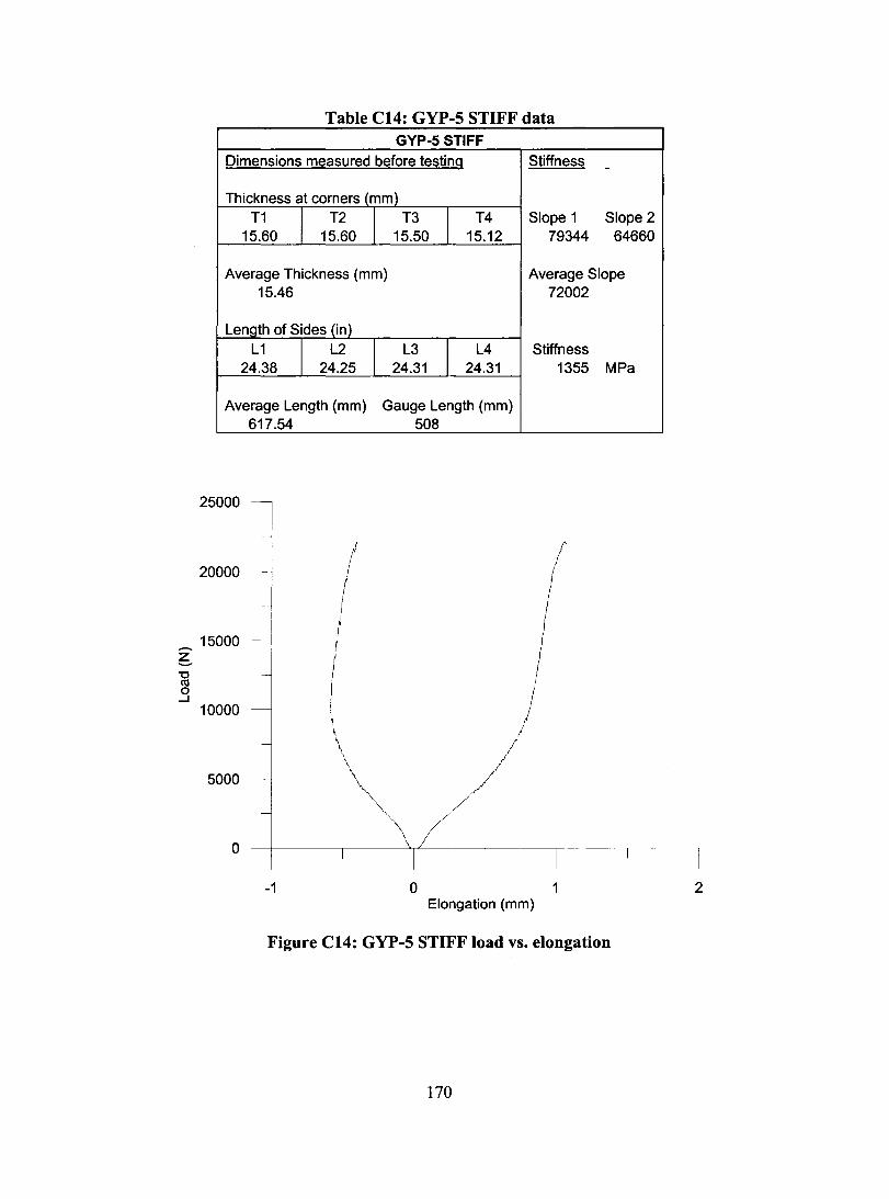
Table C14: GYP-5 STIFF data GYP-5 STIFF
Dimensions measured before testing Stiffness -Thickness at corners (mm)
T1
1
T2
1
T3
1
T4 Siope 1 Siope 2 15.60 15.60 15.50 15.12 79344 64660
Average Thickness (mm) Average Siope 15.46
Length of Sides (in) L1
1
L2 24.38 24.25
Average Length (mm)
25000
20000
_ 15000 z -"0 !Il o ..J
10000
617.54
5000 -
o
-1
72002
1
L3
1
L4 Stiffness 24.31 24.31 1355 MPa
Gauge Length (mm) 508
o 1 Elongation (mm)
Figure C14: GYP-5 STIFF load vs. elongation
170
2

z -"C ro o
..J
Table C15: GYP-6 STIFF data GYP-6STIFF
Dimensions measured before testing Stiffness
Thickness at corners (mm) T1
1
T2 1 T3
1
T4 Siope 1 Siope 2 15.28 15.46 15.36 15.24 41241 102245
Average Thickness (mm) Average Siope 15.34 71743
Length of Sides (in) L1
1
L2
1
L3
1
L4 Stiffness 24.25 24.31 24.25 24.31 1363 MPa
Average Length (mm) Gauge Length (mm) 616.74 508
25000
20000
15000
10000
5000
o
-1 o 1 2 Elongation (mm)
Figure C15: GYP-6 STIFF load vs. elongation
171

Table C16· FB+ISO 1 data FB+ISO 1
Dimensions measured before testing Stiffness
Thickness at corners (mm) T1
1
T2
1
T3
1
T4 Siope 1 Siope 2 23.44 24 24.06 24 21777 NIA
Average Thickness (mm) Average Siope 23.875 21777
Length of Sides (in)
L1 1 L2 1 L3
1
L4 Stiffness 24.3125 24.3125 24.3125 24.25 265 MPa
Average Length (mm) Gauge Length (mm) 617.1406 508
30000
~ 20000
"0 ro o
....J
10000
o --+-------,-----+-----,---,-----,---------,-----,
-1 o 1 Elongation (mm)
Figure C16: FB+ISO lload vs. elongation
172
2

Table C17: FB+ISO 2 data FB+ISO 2
Dimensions measured before testing Stiffness
Thickness at corners (mm) T1
1 T2 1
T3
1
T4 Siope 1 Siope 2 23.42 23.36 23.22 23.42 28261 NIA
Average Thickness (mm) Average Siope 23.36
Length of Sides (in) L1
1
L2 24.31 24.25
Average Length (mm) 617.93
30000 -
~ 20000
'0 ct! o
....J
10000
-1
1
28261
L3
1
L4 Stiffness 24.31 24.44
Gauge Length (mm)
o
508
1 Elongation (mm)
352
Figure C17: FB+ISO 2 load vs. elongation
173
MPa
2
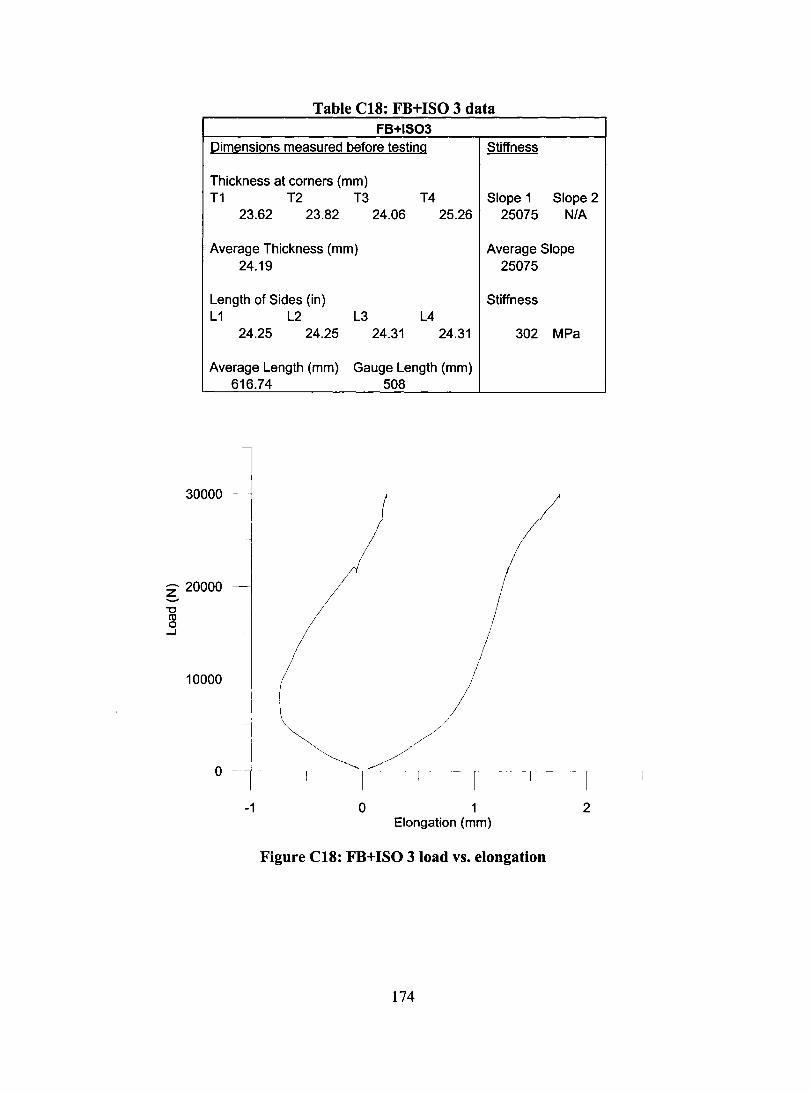
Table C18: FB+ISO 3 data FB+IS03
Dimensions measured before testing Stiffness
Thickness at corners (mm) T1 T2 T3 T4 Siope 1 Siope 2
23.62 23.82 24.06 25.26 25075 NIA
Average Thickness (mm) Average Siope 24.19
Length of Sides (in) L1 L2
24.25 24.25
Average Length (mm) 616.74
30000
Z 20000 '-"
'0 co o
....J
10000 ---
o
-1
25075
Stiffness L3 L4
24.31 24.31 302
Gauge Length (mm)
o
508
1 Elongation (mm)
Figure C18: FB+ISO 3 load vs. elongation
174
MPa
2

Table C19: FULL SECTION 1 data FULL SECTION 1
Dimensions measured before testing Stiffness
Thickness at corners (mm) T1 J T2 j T3
1
T4 Siope 1 Siope 2 23.54 23.32 24.48 23.16 32535 NIA
Average Thickness (mm) Average Siope 23.63 32535
Length of Sides (in) Stiffness L1
1
L2
1
L3
1
L4 24.25 24.31 24.13 24.38 401 MPa
Average Length (mm) Gauge Length (mm) 617.33 508
30000
Gypsum Curve /
Z 20000 -"'C Cl! o
....J
10000
o -
o
Fibreboard Curve
-j-T 1
Elongation (mm)
Figure C19: FULL SECTION lload vs. elongation
175
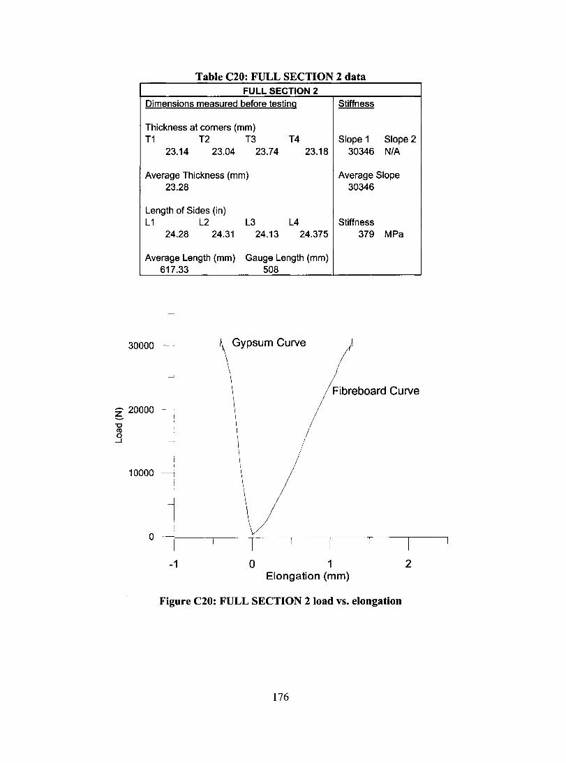
Table C20: FULL SECTION 2 data FULL SECTION 2
Dimensions measured before testing Stiffness
Thickness at corners (mm) T1 T2 T3 T4 Siope 1 Siope 2
23.14 23.04 23.74 23.18 30346 NIA
Average Thickness (mm) Average Siope 23.28 30346
Length of Sides (in) L1 L2 L3 L4 Stiffness
24.28 24.31 24.13 24.375 379 MPa
Average Length (mm) Gauge Length (mm) 617.33 508
30000 Gypsum Curve
Fibreboard Curve
~ 20000
"C ro o
....J
10000
o
-1 o 1 Elongation (mm)
Figure C20: FULL SECTION 2 load vs. elongation
176
2
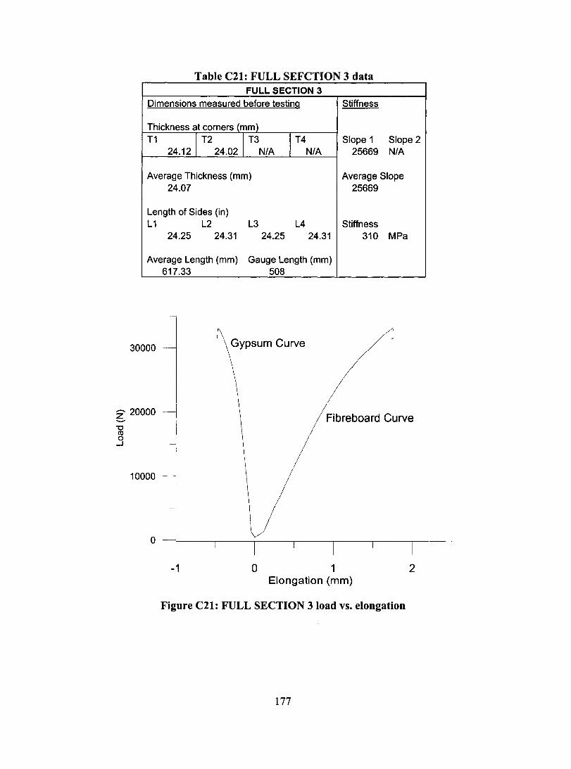
Table C21: FULL SEFCTION 3 data FULL SECTION 3
Dimensions measured before testing Stiffness
Thickness at corners (mm) T1
1 T2 1 T3 1 T4 Siope 1 Siope 2 24.12 24.02 NIA NIA 25669 NIA
Average Thickness (mm) Average Siope 24.07 25669
Length of Sides (in) L1 L2 L3 L4 Stiffness
24.25 24.31 24.25 24.31 310 MPa
Average Length (mm) Gauge Length (mm) 617.33 508
30000 Gypsum Curve
Z 20000 Fibreboard Curve -
10000
o
-1 o 1 Elongation (mm)
Figure C21: FULL SECTION 310ad vs. elongation
177
2
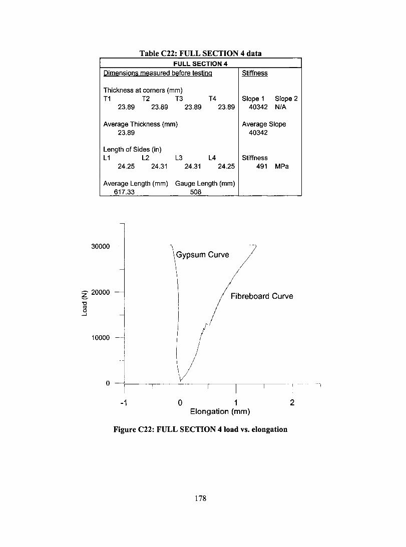
Table C22: FULL SECTION 4 data FULL SECTION 4
Dimensions measured before testing Stiffness
Thickness at corners (mm) T1 T2 T3 T4 Siope 1 Siope 2
23.89 23.89 23.89 23.89 40342 NIA
Average Thickness (mm) Average Siope 23.89 40342
Length of Sides (in) L1 L2 L3 L4 Stiffness
24.25 24.31 24.31 24.25 491 MPa
Average Length (mm) Gauge Length (mm) 617.33 508
30000 Gypsum Curve
~ 20000 Fibreboard Curve "0 CIl o
....J
10000
o
-1 o 1 Elongation (mm)
Figure C22: FULL SECTION 4 load vs. elongation
178
2

APPENDIXD
CONNECTION TEST DATA
The results of the connection tests were presented in Chapter 3, Section 3.5 and in this
Appendix. The load versus elongation curve of each specimen is shown in this Appendix.
179
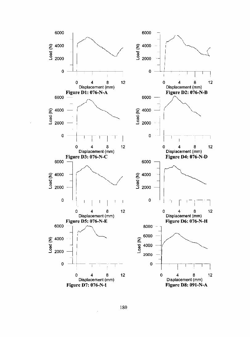
6000 6000
~ 4000 ~ 4000 "0 "0 ca ca 0 2000 0 2000 -l -l
0 0
0 4 8 12 0 4 8 12 Displacement (mm) Displacement (mm)
Figure Dl: 076-N-A Figure D2: 076-N-B 6000 6000
Z 4000 Z 4000 ........ ........ "0 "0 ca ca 0 2000 0 2000 -l -l
0 li 0 1 0 4 8 12 0 4 8 12
Displacement (mm) Displacement (mm) Figure D3: 076-N-C Figure D4: 076-N-D
6000 6000
Z 4000 Z 4000 ........ ........ "0 "0 ca ca 0 2000 0 2000 -l -l
0 0
0 4 8 12 0 4 8 12 Displacement (mm) Displacement (mm)
Figure D5: 076-N-E Figure D6: 076-N-H 6000 8000
~ 4000 - 6000 z ........
"0 "0 4000 ca ca 0 2000 0 -l -l
2000
0 -----r-~ 0
0 4 8 12 0 4 8 12 Displacement (mm) Displacement (mm)
Figure D7: 076-N-I Figure D8: 091-N-A
180

8000 8000
6000 - 6000 z z - -"'C 4000 ~ 4000 ro 0 0
...J ...J 2000 2000
0 0
0 4 8 12 0 4 8 12 Displacement (mm) Displacement (mm)
Figure D9: 091-N-B Figure DIO: 091-N-C 8000 8000
- 6000 - 6000 ~ z -"'C 4000 ~ 4000 ro 0 0
...J ...J 2000 2000
0 0 l 0 4 8 12 0 4 8 12
Displacement (mm) Displacement (mm) Figure Dll: 091-N-D Figure D12: 091-N-E
8000 8000
6000 - 6000 z z - -"'C 4000 "'C 4000 ro ro 0 0
...J ...J 2000 2000
0 0
0 4 8 12 0 4 8 12 Displacement (mm) Displacement (mm)
Figure D13: 091-N-H Figure D14: 091-N-I 12000 12000
- 8000 - 8000 z z - -"'C "'C ro ro 0 4000 0 4000 ...J ...J
0 0
0 4 8 12 0 4 8 12 Displacement (mm) Displacement (mm)
Figure DIS: 122-N-A Figure D16: 122-N-B
181

12000 12000
- 8000 - 8000 z ~ -"'0 "'0 (Il (Il 0 4000 0 4000 ....J ....J
0 0
0 4 8 12 0 4 8 12 Displacement (mm) Displacement (mm)
Figure D17: 122-N-C Figure D18: 122-N-D 12000 12000
8000 - 8000 z z - -"0 "0 (Il (Il 0 4000 0 4000 ....J ....J
0 0
0 4 8 12 0 4 8 12 Displacement (mm) Displacement (mm)
Figure D19: 122-N-E Figure D20: 122-N-H 12000
12000
- 8000 - 8000 ~ ~ "'0 "'0 (Il (Il 0 4000 0 4000 ....J
....J
0 -1 1
0
0 4 8 12 0 4 8 12 Displacement (mm) Displacement (mm)
Figure D21: 122-N-I Figure D22: 151-N-A 12000 12000
- 8000 - 8000 z z - -"0 "0 (Il (Il 0 4000 0 4000 -....J ....J
0 0
0 4 8 12 0 4 8 12 Displacement (mm) Displacement (mm)
Figure D23: 151-N-B Figure D24: 151-N-C
182

12000
~ 8000 "0 ro .3 4000
o
16000
_ 12000 ~ -g 8000 o
...J 4000
o
4000
_ 3000 ~ -g 2000 o
...J 1000
o
4000
_ 3000 ~ -g 2000 o
o 4 8 Displacement (mm)
Figure D25: 151-N-D
o 4 8 Displacement (mm)
Figure D27: 151-N-H
12
12
o 2 4 6 8 10 Displacement (mm)
Figure D29: 076-S-A
...J 1000 -
o
o 2 4 6 8 10 Displacement (mm)
Figure D31: 076-S-C
183
12000
Z 8000 -"0 ro .3 4000
16000
_ 12000 ~ -g 8000 o
...J 4000
o
4000
_ 3000 z ....... -g 2000 o
...J 1000
o
4000
_ 3000 z ....... -g 2000 o
...J 1000
o
o
o
4 8 12 Displacement (mm) Figure D26: 151-N-E
4 8 12 Displacement (mm) Figure D28: 151-N-I
o 2 4 6 8 10 Displacement (mm) Figure D30: 076-S-B
o 2 4 6 8 10 Displacement (mm) Figure D32: 076-S-D
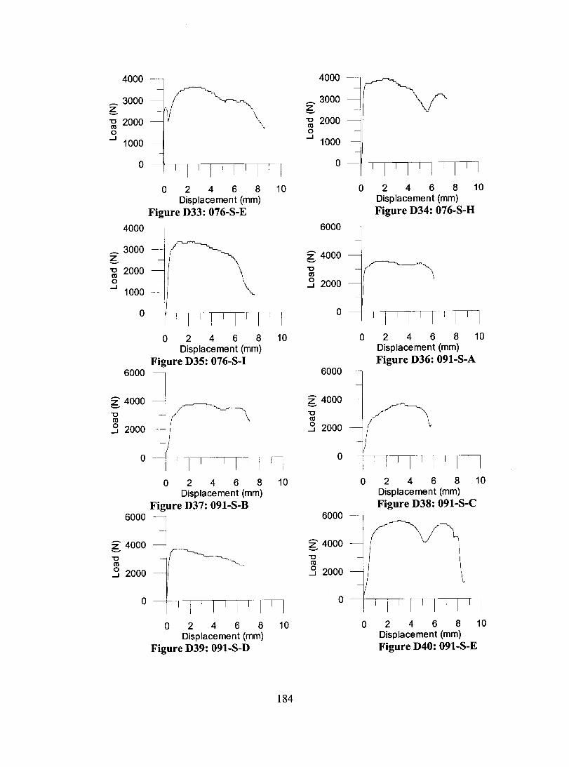
4000
_ 3000 b ~ 2000 o
....J 1000
o
4000
_ 3000 b ~ 2000 o
....J 1000
o
o 2 4 6 8 10 Displacement (mm)
Figure D33: 076-S-E
o 2 4 6 8 10 Displacement (mm)
Figure D35: 076-S-1 6000 -
~ 4000 "'0 ro .3 2000
o --t-----,--,~_,___I '--1 -'-1 --'--1 lTTl
6000
Z 4000 -"'0 ro .3 2000
o
o 2 4 6 8 10 Displacement (mm)
Figure D37: 091-S-B
o 2 4 6 8 10 Displacement (mm)
Figure D39: 091-S-D
184
4000
_ 3000 b ~ 2000 o
....J 1000
o
6000
~ 4000 "'0 ro .3 2000
o
6000
~ 4000 "'0 ro .3 2000
o
6000
Z 4000 -"'0 ro .3 2000
o 2 4 6 8 10 Displacement (mm) Figure D34: 076-S-H
o 2 4 6 8 10 Displacement (mm) Figure D36: 091-S-A
1 1 1 1 1 1
o 2 4 6 8 10 Displacement (mm) Figure D38: 091-S-C
o 2 4 6 8 10 Displacement (mm) Figure D40: 091-S-E
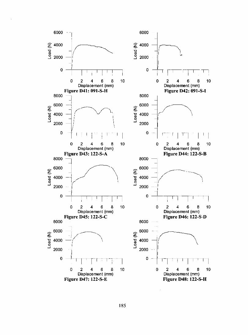
6000
~ 4000 "0 CIl
.3 2000
8000
_ 6000 6 ~ 4000 o
....J 2000
o
8000
_ 6000 6 ~ 4000 o
....J 2000
o
8000
_ 6000 6 ~ 4000 o
....J 2000
o 2 4 6 8 10 Displacement (mm)
Figure D41: 091-S-H
o 2 4 6 8 10 Displacement (mm)
Figure D43: 122-S-A
o 2 4 6 8 10 Displacement (mm)
Figure D45: 122-S-C
o 2 4 6 8 10 Displacement (mm)
Figure D47: 122-S-E
185
6000
~ 4000 "0 CIl
.3 2000
8000
_ 6000 6 ~ 4000 o
....J 2000
o
8000
_ 6000 6 ~ 4000 o
....J 2000
o
8000
_ 6000 6 ~ 4000 o
....J 2000
o 2 4 6 8 10 Displacement (mm) Figure D42: 091-S-1
o 2 4 6 8 10 Displacement (mm) Figure D44: 122-S-B
o 2 4 6 8 10 Displacement (mm) Figure D46: 122-S-D
o --~~~~~~~~~
o 2 4 6 8 10 Displacement (mm) Figure D48: 122-S-H
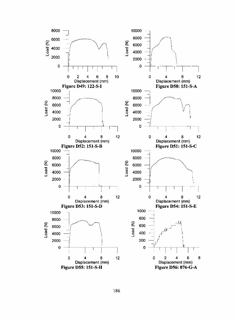
8000
.- 6000 ~ ~ 4000 o
....J 2000
o
10000
8000
~ 6000 "0
~ 4000 ....J
.-
2000
o
10000
8000
~ 6000 "0
~ 4000 ....J
.-
2000
o
10000
8000
~ 6000 "0
~ 4000 ....J
2000
o
o 2 4 6 8 10 Displacement (mm)
Figure D49: 122-8-1
il o 4 8 12
Displacement (mm) Figure D52: 151-8-B
o 4 8 12 Displacement (mm)
Figure D53: 151-S-D
o 4 8 12 Displacement (mm)
Figure D55: 151-S-H
186
10000
8000 .-~ 6000 "0
~ 4000 ....J
2000
o
10000
8000
~ 6000 "0
~ 4000 ....J
2000
o
10000
8000 z - 6000 "0
~ 4000 ....J
2000
o
1000
o 4 8 12 Displacement (mm) Figure D50: 151-8-A
o 4 8 12 Displacement (mm) Figure D51: 151-S-C
o 4 8 12 Displacement (mm) Figure D54: 151-S-E
800 -
~ 600 "0
~ 400 ....J
200
o
o 2 4 6 8 Displacement (mm)
Figure D56: 076-G-A
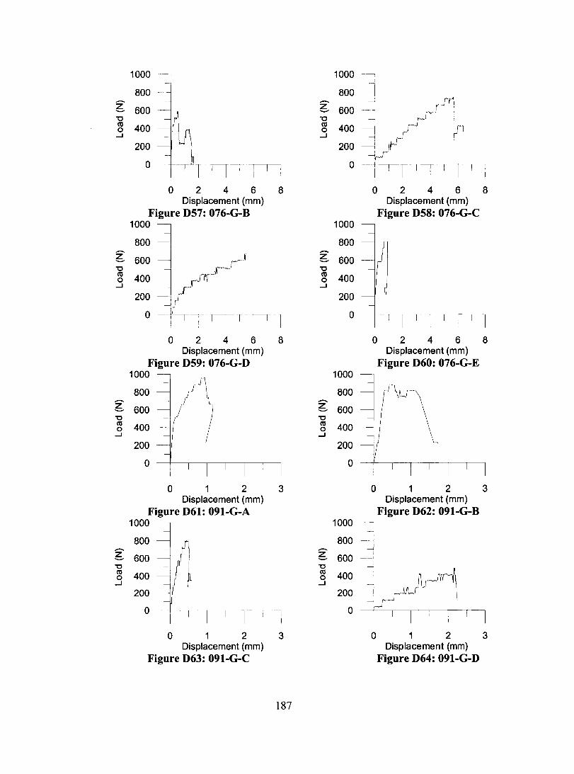
1000 1000
800 800 Z 600 Z 600 - -"0 "0 ct! 400 ct! 400 0 0
....1 ....1
200 200
0 0
0 2 4 6 8 0 2 4 6 8 Displacement (mm) Displacement (mm)
Figure D57: 076-G-B Figure D58: 076-G-C 1000 1000
800 800
~ -600 ~ 600 "0 "0 ct! 400 ct! 400 0 0
....1 ....1
200 200
0 0
0 2 4 6 8 0 2 4 6 8 Displacement (mm) Displacement (mm)
Figure D59: 076-G-D Figure D60: 076-G-E 1000 1000
800 800
~ -600 ~ 600 "0 "0 ct! 400 ct! 400 0 0
....1 ....1
200 200
0 0
0 1 2 3 0 1 2 3 Displacement (mm) Displacement (mm)
Figure D61: 091-G-A Figure D62: 091-G-B 1000 1000
800 800 - -~ 600 ~ 600 -"0 "0
nr1 ct! 400 ct! 400 0 0 ....1 ....1
200 200
o --I~I------r-~ l------r---1 0 li
0 1 2 3 0 1 2 3 Displacement (mm) Displacement (mm)
Figure D63: 091-G-C Figure D64: 091-G-D
187
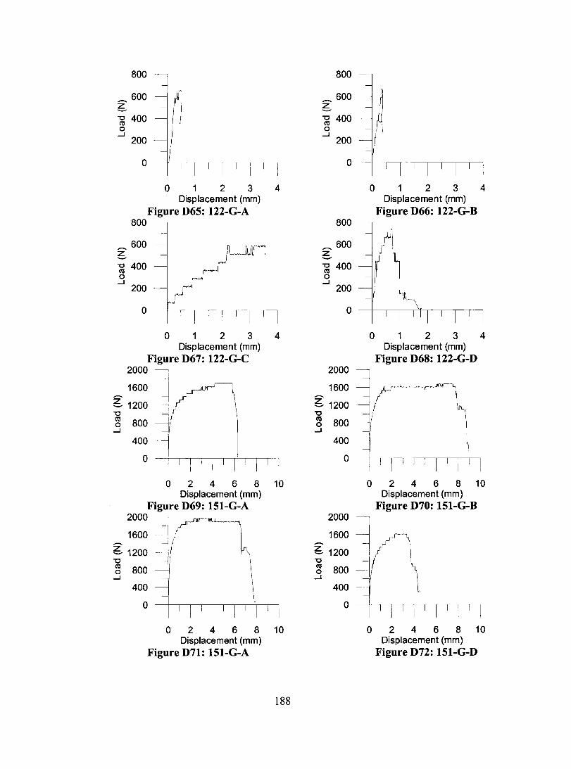
800
_ 600 ~ "0 400 co o
...J 200
o
o 1 234 Displacement (mm)
Figure D65: 122-G-A 800
_ 600 ~ "0 400 co o
...J 200
o
o 1 234 Displacement (mm)
Figure D67: 122-G-C 2000
1600
~ 1200 "0
~ 800 ...J
400
o
o 2 4 6 8 10 Displacement (mm)
Figure D69: 151-G-A 2000
1600
~ 1200 "0
~ 800 ...J
400
o
o 2 4 6 8 10 Displacement (mm)
Figure D71: 151-G-A
188
800
_ 600 ~ ~ 400 o
...J 200
o
800
_ 600 z -"0 400 co o ...J
200
o
2000
1600
~ 1200 "0
~ 800 ...J
400
o
2000
1600
~ 1200 "0
~ 800 ...J
400
o
1 1 1 1 1
o 1 234 Displacement (mm)
Figure D66: 122-G-B
o 1 234 Displacement (mm)
Figure D68: 122-G-D
o 2 4 6 8 10 Displacement (mm)
Figure D70: 151-G-B
o 2 4 6 8 10 Displacement (mm)
Figure D72: 151-G-D

APPENDIXE
SAP2000 INPUT/OUTPUT FILE EXCERPTS
The analytical results are presented in Chapter 4. Excerpts of the input and output files of
the 38-76-6-NS-R-M models are shown in this Appendix. AH input files and output files
are similar therefore only this model's input and output files are shown.
The actual input file for the 38-76-6-NS-M model is 1009 pages long and the output file
contains more than 5000 pages. Therefore, only excerpts of each section of the input and
output files are presented in this Appendix. AH tables are unformatted, therefore not
included in the List of Tables.
For the input, sample node, element and link definitions are be presented.
For the output, sorne sample node deflections and element stresses are presented.
189

FOR MODEL 38-76-6-NS-R-M
INPUT:
File G:\Thesis\SAP\Finals\With Roofing\076\38-76-6-NS-R-M.$2k was saved on 10/10/05 at 22:28:44
TABLE: "JOINT COORDINATES" Joint=l CoordSys=GLOBAL CoordType=Cartesian XorR=482.6 Y=O Z=0.5 Joint=2 CoordSys=GLOBAL CoordType=Cartesian XorR=514.35 Y=O Z=38.1 Joint=3 CoordSys=GLOBAL CoordType=Cartesian XorR=482.6 y=101.6 Z=0.5 Joint=4 CoordSys=GLOBAL CoordType=Cartesian XorR=558.8 Y=O Z=38.1 Joint=5 CoordSys=GLOBAL CoordType=Cartesian XorR=603.25 Y=O Z=38.1 Joint=6 CoordSys=GLOBAL CoordType=Cartesian XorR=615.95 Y=O Z=O Joint=7 CoordSys=GLOBAL CoordType=Cartesian XorR=635 Y=O Z=O Joint=8 CoordSys=GLOBAL CoordType=Cartesian XorR=654.05 Y=O Z=O Joint=9 CoordSys=GLOBAL CoordType=Cartesian XorR=666.75 Y=O Z=38.1 Joint=10 CoordSys=GLOBAL CoordType=Cartesian XorR=711.2 Y=O Z=38.1 Joint=ll CoordSys=GLOBAL CoordType=Cartesian XorR=755.65 Y=O Z=38.1 Joint=12 CoordSys=GLOBAL CoordType=Cartesian XorR=768.35 Y=O Z=O Joint=13 CoordSys=GLOBAL CoordType=Cartesian XorR=787.4 Y=O Z=O Joint=14 CoordSys=GLOBAL CoordType=Cartesian XorR=806.45 Y=O Z=O Joint=15 CoordSys=GLOBAL CoordType=Cartesian XorR=819.15 Y=O Z=38.1 Joint=967 CoordSys=GLOBAL CoordType=Cartesian XorR=25.4 y=50.8 Z=-0.5
TABLE: "CONNECTIVITY - FRAME/CABLE" Frame=l JointI=967 JointJ=968 Frame=2 JointI=968 JointJ=969 Frame=3 JointI=969 JointJ=970 Frame=4 JointI=970 JointJ=971 Frame=5 JointI=971 JointJ=972 Frame=6 JointI=972 JointJ=973 Frame=7 JointI=973 JointJ=974 Frame=8 JointI=974 JointJ=975 Frame=9 JointI=975 JointJ=742 Frame=10 JointI=742 JointJ=741 Frame=ll JointI=741 JointJ=724 Frame=12 JointI=724 JointJ=725 Frame=13 JointI=725 JointJ=726 Frame=14 JointI=726 JointJ=727 Frame=15 JointI=727 JointJ=728
TABLE: "CONNECTIVITY - AREA" Area=l Joint1=460 Joint2=461 Joint3=946 Joint4=947 Area=2 Joint1=461 Joint2=462 Joint3=947 Joint4=948 Area=3 Jointl=462 Joint2=463 Joint3=948 Joint4=949 Area=4 Joint1=463 Joint2=465 Joint3=949 Joint4=950 Area=5 Joint1=465 Joint2=466 Joint3=950 Joint4=951 Area=6 Jointl=466 Joint2=951 Joint3=467 Joint4=952 Area=7 Joint1=467 Joint2=468 Joint3=952 Joint4=953 Area=8 Joint1=468 Joint2=469 Joint3=953 Joint4=954 Area=9 Joint1=469 Joint2=954 Joint3=470 Joint4=955 Area=10 Joint1=470 Joint2=471 Joint3=955 Joint4=956 Area=ll Joint1=471 Joint2=472 Joint3=956 Joint4=957
190

Area=12 Jointl=472 Joint2=473 Joint3=957 Joint4=958 Area=13 Jointl=473 Joint2=474 Joint3=958 Joint4=959 Area=14 Jointl=474 Joint2=475 Joint3=959 Joint4=960 Area=15 Jointl=475 Joint2=960 Joint3=476 Joint4=961
TABLE: "CONNECTIVITY - LINK" Link=l JointI=36442 JointJ=36462 Link=2 JointI=25252 JointJ=25272 Link=3 JointI=947 JointJ=967 Link=4 JointI=14062 JointJ=14082 Link=5 JointI=47372 JointJ=47427 Link=6 JointI=36182 JointJ=36237 Link=7 JointI=462 JointJ=489 Link=8 JointI=460 JointJ=487 Link=9 JointI=461 JointJ=488 Link=10 JointI=24992 JointJ=25047 Link=l1 JointI=13802 JointJ=13857 Link=12 JointI=687 JointJ=742 Link=13 JointI=467 JointJ=490 Link=14 JointI=468 JointJ=491 Link=15 JointI=469 JointJ=492
191
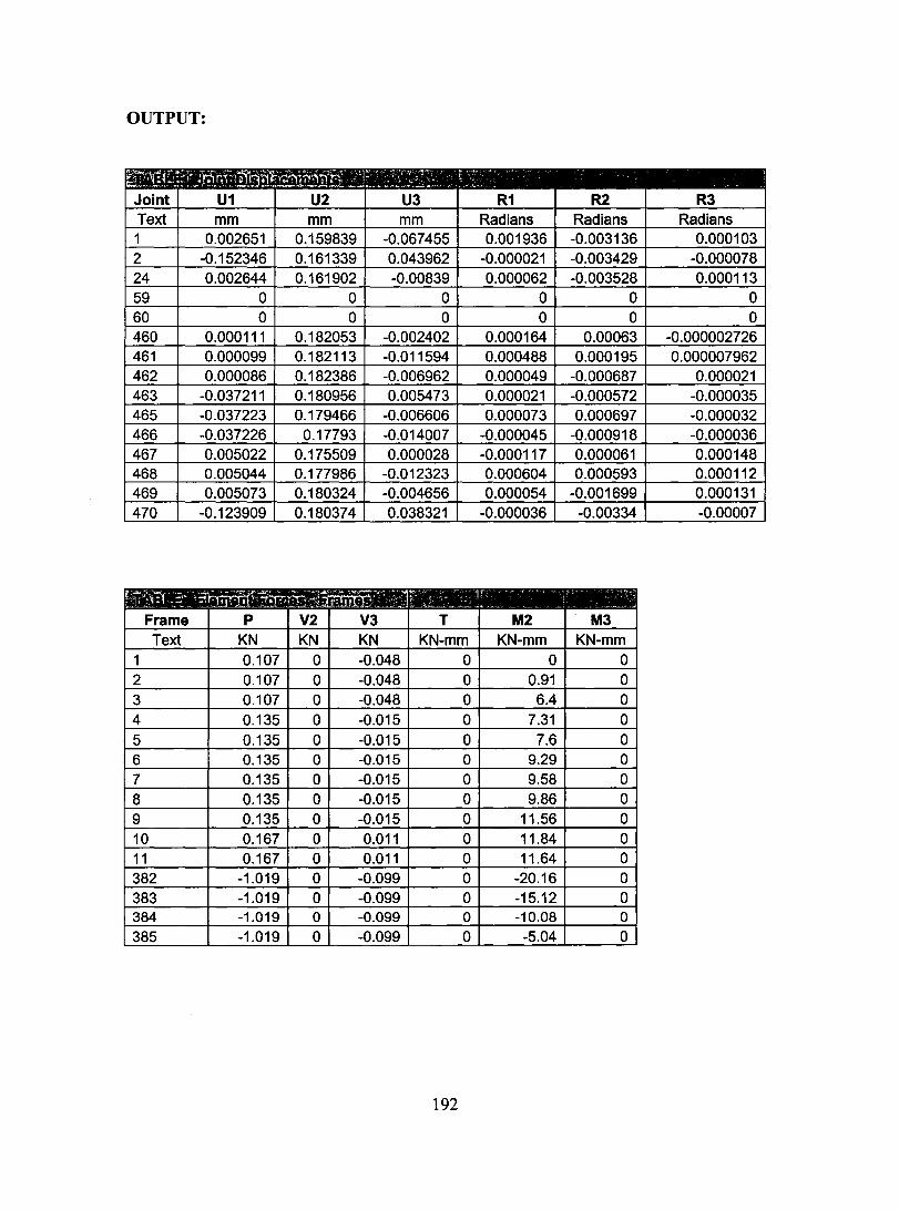
OUTPUT:
e~~:r ,,"' ~.. . ë\î- lf.t;;::?t p' - '.' .~'" «. -- "' • .. -' -,
~~: _ :':":t_·JF!\[;f~~~I)!1.~~...-'i!lUn _~~.~ .:':L;':"';: .. , .~.,;"" . Joint U1 U2 U3 R1 R2 R3 Text mm mm mm Radians Radians Radians 1 0.002651 0.159839 -0.067455 0.001936 -0.003136 0.000103 2 -0.152346 0.161339 0.043962 -0.000021 -0.003429 -0.000078 24 0.002644 0.161902 -0.00839 0.000062 -0.003528 0.000113 59 0 0 0 0 0 0 60 0 0 0 0 0 0 460 0.000111 0.182053 -0.002402 0.000164 0.00063 -0.000002726 461 0.000099 0.182113 -0.011594 0.000488 0.000195 0.000007962 462 0.000086 0.182386 -0.006962 0.000049 -0.000687 0.000021 463 -0.037211 0.180956 0.005473 0.000021 -0.000572 -0.000035 465 -0.037223 0.179466 -0.006606 0.000073 0.000697 -0.000032 466 -0.037226 0.17793 -0.014007 -0.000045 -0.000918 -0.000036 467 0.005022 0.175509 0.000028 -0.000117 0.000061 0.000148 468 0.005044 0.177986 -0.012323 0.000604 0.000593 0.000112 469 0.005073 0.180324 -0.004656 0.000054 -0.001699 0.000131 470 -0.123909 0.180374 0.038321 -0.000036 -0.00334 -0.00007
192

193
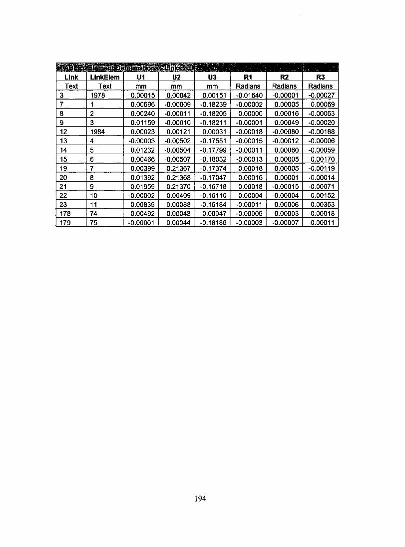
'~I\':r"·'''·<~!:B:l: . _ .. ~~.<."~ .. , , .. '. ., .. r"'[f" ~~~-, ~ ~%J~-. ~-, ~, - , , . ~<'.,~._....... . 8!ût1 ;.;-~.,._"_ ~ ~ .. ,' ~ ~ '" ~ >: -" ''''-- - . .
Link LinkElem U1 U2 U3 R1 R2 R3 Text Text mm mm mm Radians Radians Radians
3 1978 0.00015 0.00042 0.00151 -0.01640 -0.00001 -0.00027 7 1 0.00696 -0.00009 -0.18239 -0.00002 0.00005 0.00069 8 2 0.00240 -0.00011 -0.18205 0.00000 0.00016 -0.00063 9 3 0.01159 -0.00010 -0.18211 -0.00001 0.00049 -0.00020 12 1984 0.00023 0.00121 0.00031 -0.00018 -0.00080 -0.00188 13 4 -0.00003 -0.00502 -0.17551 -0.00015 -0.00012 -0.00006 14 5 0.01232 -0.00504 -0.17799 -0.00011 0.00060 -0.00059 15 6 0.00466 -0.00507 -0.18032 -0.00013 0.00005 0.00170 19 7 0.00399 0.21367 -0.17374 0.00018 0.00005 -0.00119 20 8 0.01392 0.21368 -0.17047 0.00016 0.00001 -0.00014 21 9 0.01959 0.21370 -0.16718 0.00018 -0.00015 -0.00071 22 10 -0.00002 0.00409 -0.16110 0.00004 -0.00004 0.00152 23 11 0.00839 0.00088 -0.16184 -0.00011 0.00006 0.00353 178 74 0.00492 0.00043 0.00047 -0.00005 0.00003 0.00018 179 75 -0.00001 0.00044 -0.18186 -0.00003 -0.00007 0.00011
194

APPENDIXF
SDI CALCULATION EXCEL WORKSHEETS
The computed values for the diaphragm stiffness using the SDI equations are presented in
Chapter 4, Section 4.5.1. The calculation sheets used to compute the stiffness of the
diaphragm are presented in this Appendix.
195
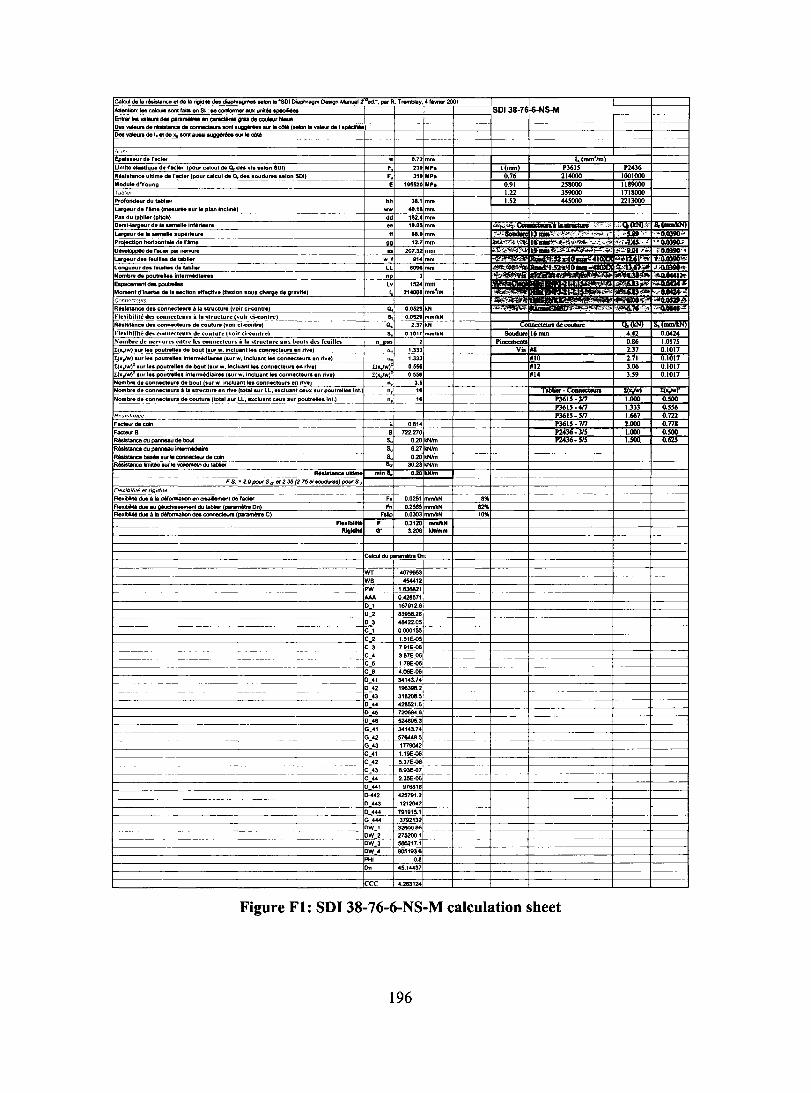
• la no.'. _ . "SOI DIa ..... m OOOign Manual rode. "'" R. Hem"'y, 4 ,.,.... 200' ...... 1ion: ... _oonc' ... ..,SI , __ en ....... valMndll __ on ~_,
"""va,"""de, • __ ou<lecOlé('-lava_det_ Ilesva .... d.~de-"'_ • .,..;_ou< .. _
u"' Épal ... u, do l'oc'" •• 7: mm Limite .... tiqu. d. l'oc", (pou, .. Icul da a. da •• 1 ••• Ion SDi) F, MP. P3615
, do l'oci., • a. do •• oudu ..... Ion SOI) F. 310 MP.
"''''' MPo L,!>r", P,ofond .. , du lablie, hh 3.. mm La, ... , d. , ..... (m".'" .uli, plan incll"') ww 40." mm P •• du t.bll.' (p"ch) dd ,.2. mm
"a, .. 19 .• ' mm L""au, do 1. , .... mm Projection honzon .... da ".... •• 12.: mm
,,"""'........... os 207. mm _.,
~~=~:~~U:~.~· .. pou'~~ ... ~_::,: .. 'do~.·::.I'~·:~·:·bi~'''~I., .. ~.~~~~~~~====E== wni·p~~~:~~E==~.~· ~ . . ".' '.
~omen. d'In.rtie do 1 .... Oon eff",' •• (".'on sou. ch .... d •• , .... ) ::()I1I1,Vt'~!HS
IR .... ...,c. d •• connee ...... ,. ,,,"C'U,, ('01, cl-con ... ) a. ...... 1'. '·'ulbm •• d" ,onnecte.,," ., .. ".<I.,e . • .• mlmm"'.
IR ...... nee_con~ .. u .. d.cou.u .. ( ... 'cl.co_) ,0. ~371.N kNJ • .,,,Ibill", • dHO.'Ul< ('0;' o;-<onll.) S. ..1." ImmlkN SoucI ... 16 mm
INomb .. d,' ..... ,,, en ... ,,~ ,0nn«I<.'" • la "IO"U" a.x bo.h d .. reuUl,~ • po. Pineomen. 1I( .. /w) .ull .. pou ... ,ta. de houll ,la. ecn~"u ... n "".) " '.333 ~ ~ lI(x,./w).u, la. pou ... ,Ia. in"~,,,.I ... (OUI w, inelu.n."', " ... ) " .33: IMIO IIj',./w)' .u' la. poullOl". d. bout (.u, w, Inc'uant Ia .. onnee"u, .. n ,"'.) I(x,./w)' ,.... I~I; I(',./w)' .u' , •• po .... , ... in'a ... "'.'".(.u, w. lnelu.n' la. connacteuII.n rive) I(.,./w)' ..... IN14 INomb .. d., • hou' ,.U, w. Incl •• n.' IOn "".) n. -,.'
"""""J O.
o. O. 0,
f.1.om~b .. ~.~ .. '~'con~MC .. ~u"'~r.".~ .. Nct~ ... '~'.n'"~y.'~.o .. ,"~'U"~LL", .. ~eiu~.n •• ee~u.'~ •• "po~U."~"~ ... "M~===~ .. ===~"====t=====+=====t::T~~~ ~~~~~~~~~~~~~ !"omb'. dOl ocoutu .. "0 •• 1 .U" .... Iuanteeux OUI pou" ..... Int. n."
IF_8
• ou<" oonneeIeUI do_ ' ........... du .. _ _tance .....
s.. s.. s.. ..
m'." F.S.-2.0 ..... S" .. 2.35' 1.7' 'S,
IFlexib"". el ".'rl'" '1a"'~Iion..,,·
'dul .Ia, 'CI
F. Fn
FSI<> F ... _I F
ftig_1 O'
0 .• 14 722.270
0·201·Nlm 6,271.NIm
··201·Nlm JO.23 1kN1m
0"'1'"""
0.0251 ImmlkN 0.2585 ImmlkN 0.OJ03 ImmlkN
3.2OIl ,"""m
,"",",du ,,,-'1
IWl 407"" IWB. 454412 IPW 1.636821 lMA 0.'2.571
'6791 . _2 • 3~2.
." 82% '0"
4 .. 22 ...
~ .. ~-------------------------------------~~~~~~--~----~-----+-------------+-----+-----1
_2 I.51E-<>. _3 r.91§.-06 _4 '.,7E-06
-' .79E-06 _6 4.06E-06 _41 34143.74 _42 196398.: _43 318208.: . 44 42852' . _45 7_ .. _4. 52481i5. ,_4t 34143.74 ,_42 .7 ...... : ,43 rl9042 _41 .19E-06 _42 ~-06 _43 •. 9JE-<>7 .44 2.35E-06 _441 9788t.
1""""" ~ _44' '212042
444 79'91'. ---,_444 3792132
IOW. ~ .. IDW. '75200. IDW_ 586211. low 4 Il00193.6 IPHI O .•
IOn 4'.14437
4.263t24
Figure FI: SDI 38-76-6-NS-M calculation sheet
196

::a,,",de~ , ,la ,,"d"_, ,,. "SO. O~"""m Des"" Manua':r'ed.', pa< R. Tremblay, •• _ 200'
IAllenI'o,,, ... """uIo ""'. fft en S, , .. _"'"* 0'" I;UI38,91 .lj,NS-M ~ ~ dao pora_ on _ groo cie couleur bleue
'''''''lance'', •• _ ..... _(_~ ......... _
1~· .. •· ...... sonIa ... '._ ... ,._ ._.
,."" lEp."".' de "",,10, O .... Imm (mm'Im)
.... rK .... 'po", c.'"", da a, .. , vi, lO'on SOI, F, 230 IMP, "",,) "" IR'.' •• anes .Olm. da rKI .. ,pou' calc.1 d. a, da, ,o.d.~, ,.ion SOI) F. 310 IMP, .76 IMod.,. d'Yo.ng .197000 IMP, '.91 18,2 IT .. '''"" ,""10, hh 3!, lm", La, .. u, da " .... (m"u'" .u, le plan InCil",) ww 40.1' Imm IP •• du ,.bila, (pitch) dd 152,' Imm
~ "","~, da..'! .. m!"a ln ....... ' •. .. ".05 Imm L .... u' da 1. _'le .... "" ... ".' Imm "". ." "
:~:.=::.~=:.~~. gg 12. Imm f.=: .. 207. Imm .• c' ,V' ,_' '."C. .' r ""g •• , d •• fouilla. da tab'lo, w ". Imm
Long ... , d •• f •• illa. da ',bl;', .... Imm ,,","'''''c
Il INomb .. da po., .. IIa. 'n'.,,"'dl.I ... np ~
;1 ~ Espacemen' dao ......... 1524 Imm 'iir·""CIiotI j".""" ",-' , .... _tian' 1 cha' .. d. g'av.') ~
(' .. """.".""" '-~""-,,,,~
"'" '.41 ,kN ...-"....""''''' .'I .. ihlli,é d .. conn",'eu" à la, • c1-con',,) S, 0.0472 mm"'N
Q, I.37,kN N) ISo tN) ..onibllit. de> co •• ",teu" de co.,.,. s. O ..... 'mm"'N - 16 mm Nomb .. de nccv.'", cn'" , \. ",.ct ..... , bu." d .. I •• illes n po> Pinc:emenll I(.Jw) .u, la. po ..... ," d. bout (.u, w, Incluant 10. ' "lva) a, ),333 Vil III! I('Jw) •• , la, po.t"''', , " Inc'uant le. connect ..... n ,Iv., o. '.333 Il!,Iw)"'" 10. ~ ... , ..... bou' (.u, w, Incluant'" connKtau .. an ... ) lOI"""')' O .... \2 I(x,Jw)" .u, la. pou .. '''' In""'OOI.I ... (.u' w, Incluant ... , "lva, lOI...".,' O .... 1. No,nb .. da connecta ... de bou' (mw, Incl •• nt"" , riv" 3.1 Nomb .... conOK"." ..... "'ct ... an rive ('otal ,." ",' •• n' es •••• , po ........ In' n. fi
Nomb,. da connecta ... da ,outu .. (total t co •• •• , ... " ..... Int., .n, -'!
R.",'."ce Fad ... de_ O." F ....... ".47E Rés~lance du panneau de ..... "- 23.80 kNim Réslslancedu __ •
. "- "." kNIm . Réslslance"'" '"" ,- "- 10.80 kNim R .... lance .. _ lU< le .. 35." kNim ...........
F.S .• 2.0pou< S •• <2.35, '.7501 ........ ) ...... S.
FI"",-bil'''-'-'''g"",, Fie'''''' dua' la ""_lion, 'r ..... F. 0.0191 mmlkN 10% - ._.-F","'Héd .... , .• ( .... """"'On\ J" _0.14:17 m .... N 75% Fie ...... duo' la """"""lion deolXlMadeuB (para"""'" C) F"~ 0.0270 mml1<N 14%
FieSlOt ... 0.1"" ....... Rigld" G' '.247 ......
cale .. d. 1 ... m'"
4079953
f---- ._--~ '544" 1.161521
MA 0.428571 16791
'_2 !..,...~
41422.0' 0.000155
"51E ... .3 7.91E"" -,_.
!.57E""
f--------- . 5 .rge .... , 6 ~~~ '.41 34143.74 '_42 1!I6391,
'-" 316201.
'." 421521.'
'.45 720664.' '.41 524695.
'_41 34143.74
' .. : 576448.,
'-'3. -'-"00.2 .41 .1BE""
'.s.. 5.37E"" _43 6.93E-07 _ .. 2.35E""
'-~ 976616 0-«2 '21791.
,_ .. ~ ~1204~
. 444 791915 . 444 ...:l792~
OW_2. '11528" OW_3 401799 OW. 642343.: PHI O.,
On 32.03535
'.615718
Figure F2: SDI 38-91-6-NS-M calculation sheet
197
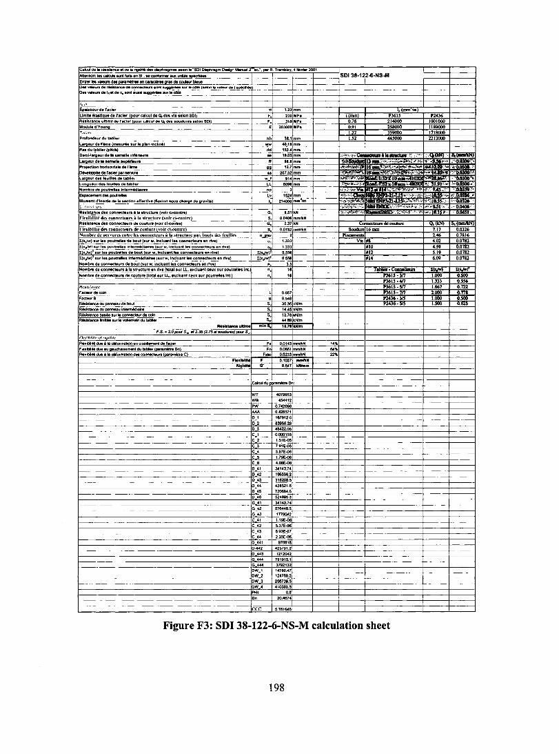
lcalcul de la, ,la ,;gd ........................ ,. "SO' Oia_m Des"" Manua' Z-o<!.', po, R. nomblay, ,,_ 200' 'U
, .......... ,.-1000 ......... ' ... ""-... -._. __ ..... _
[E;~.~rd~,~--------------------------~----r-~I~,,"~[m~m~~--~-----+------TJ'-=mm,~c~~----f---~ Limite .... tlqu. d. "ader (pou, e.'eu'de a, de. v" .o'on SO'j F, IMP. IR"'slance u"'m. de "ac'.r (pou, cafeu' de , ,do •• oudu ... se'on SOI) -", J10 IMP' [Modu', d'Young 2.JOOOIMP,
"ab'ler hh 3 •. [mm
, roonee"u" d, cou'ure ('01, ';-<on".) S. • .• 7.' Imm"'" [Nombre de ne<vu,,, ,n", I,~ eonnecteu" • ,. "ructure aux bou" d,~ reulll,~ n"po> t(x,/wj'u' le. pou""1es de bou' (.u' w,'nc'uan' le. conneeteurs on rivo) 0, 1.33: [""".,) .u, 'o. pou,,,"" 'nte .. Id'.,,,. (.u, w,'nc'u.n' ,on ,",,' 0, 1.333 Ej',lwj' .u, 'o. pou ... 'Io. do bout (.ur w, 'nc'uant les H'VO) t(x,/w)' ..... [t(.".,j' su, , .. po .... ,Ie.; , 'W, 'ncluan' les connecteurs.n rivej EI.".,j' O .... INomb .. , , de baufl.u, w, 'nclu.ntl.sconneeteurs on rive) n. 'Nomb .. ' ",. s.ructu .. en ov. ('0'" .ur' ... ,,'uanl ceu. sur pou"Oi' .. ,nl: n. ,Nomb,., • decoulU .. (lol,"u" , .. e'u,ntc,u"ur~u"OiIe.Int.: n,
Foct ....
,. ,. ).857 . ....
iR"isIance du",,"",,"u do bout s.. 35.'5 [kNim R_lance du ponnoaulntennédlslr. Résistance ..... sur" connecteu< .. _
."''',nce lm'" sur iOiOiiiiiietn~ F.S . • 2.0 pour S. of 2.35 (2. 70" _si pour S,
FI."b,'''' ct "u,d", Fie"",,! d ... 1
FIe' ..... d ... ,
--_.
-
-.
-
,""_de~ .du .. _( .......... Onj
'Ie ....... RIg""
s.. ''''5 kNim s.. 1.7.kNlm
'" ..... ,'N1m ',7I'kNhn
-", 0~43 m""'~ Fn 0.0861 ..-"
Fs .. 0.0233 m""'"
• 0.1037 mmIkN O' 9.847 kNhnm
[ca .... du po ...... On,
[WT 4079953 IW. .... ,2 [pw 0.742096 IAM 0.428571
167912.6 2 !3956.2.
-' 484".05 0.000155
..2. I."E-O • ' .• 'E-O J.57E-OS
-' '.79E-OS _6 4.06E-OS _41 34143.74
196398.: _43 31B208-' _44 428521. _45 720864. _46 .2 ..... :
~'- 34143. _42 578448.' 43 ln""
1.19E'" 42 5.37E'"
:_43 B.93E-O) .44 !.35E'"
'_441 9768" 0 .... 2 425791.
_443 1212042
_444 7.'~'~. _444 >7921:
OW. 14780.' OW_2 124769.: OW..3.. ?~.! ,OW_4 410393.' ,PHI O .• On 20."7<
'.76184'
,.,, 84" ..,.
mm
',91 .22 ,,li
Vis N8 NIO NI: N14
,..,,, .. -<.:-
Figure F3: SDI 38-122-6-NS-M calculation sheet
198
-
P2436
18000 1l'lOO_
r-- - ,-

1"""" ............ nco ..... Ia .. ~ .. , 'Manue' '·od.', pa< R. ,20(11
,5DI38 0 1S11-6o NS-M IAttention, ieo .. IcuIo"'"" ...... S', .. """""""'.ux ................
~:.. "":"'...:.==:...... __ ... "'cOIt 1'-" .. _det"""'"
IDes ....... del, .. de ... _."""_ .... locOlt
14.,", IEpa' ••• U' do "oclo, 1." ,mm I,(mm'/m) Llm' ...... tlqu. d. "ocle, lpou, <o'eu' de a, de •• , ••• 'on So'l FJ _230 '",Pa P36IS '2436 1.4.,.t.ne. u",ma de "oc,., (pou, ca'eu' d. a. de •• oudu~ •• o'on SO', 310 MP. 1.76 214000 101000 'Modu'. d'Young 'O!OOO ",Pa 189000 T"U,-, 3~9000 ,.8000 'P,ofond .. , du tab'le, "" 3 •. 1 mm L .... u'de , .u' la plan Inc"") ww 40,16 mm P,. du t.bllo' (D"ch) d' "2,' mm
".- .. 1.,0' mm .... _,. <hlOH' , L ..... 'd.l. _ .... n'm
B P~joet;on hon.ontale do "am. •• 12: mm ".c, . -."""""..,,,c " ...... par noMKa .. 207.3' mm k'i L ...... ' de. f.ulll .. de "b'le, w, "4 mm
Longu.u' do. foull". do t.bllo, 1096 mm !é",~.?,,,"C;;,
Nombre do pou ... 'Ie.lnt.~..".;'o. n,
.""" ..... L, 1524 mm "~>'dJIII M~ntd .... rt;;' dOl. section offectl,o (n."on .ou. ch'fII. d. g'''''') ~.,'t",. ~ :''''''''','',,,", , .. }.' .60' ... nco da. connoctou ... la .uuclu,. ('0" cl-con"', a, '.41 kN "',,'hilil' , , la ,"uctu .. ("01, cI"",n"c) O,OllS mm,.N ."'."nc. _ connec ..... d. cou'u .. ('0" e'-contr.' Q, '.37 kN ~ ,<NJ 1" (tDDIfltNJ "I.,ibm .. , • de coutu" (.oi, "-<on"., S, 0.0703 mm"N Soudure l6aun 0,0293 Nomhre d. nc!"Vu,.., en"e 1.., connecteu" » la ",ucture aux houlo d" r.uill" n Da, I(xJw) .u, ,.. pou .... ,.. da bout 1 t le. connac .. u .. en "'0) ., Vis liN! 0,0703
,p) .u, , •• poutrel". 'n .. ~Sd' .. ro. (.u, w,'nc'uant les, , 'lvo) 0, '.333 I( • .Iw)' .u, ........ 1reIIo. de -"""' (su, w,lnclu.nt ,.. , HOVo) I(sJw)' o .... lOI: 0.0703
,Pl" 'u'''' pou ... , ... lnt.onSdI.I ... (.u, w,lnclu.nt' .. n"'.) "",)' o .... 1014 53 0.0703 Nombre de connect.u .. da bout (.u, w, Incluant •• n"'o) " Nombre do connoc ...... " IINetu ... n rIv. (tota' .u, LL, exc'uent coux su, pou'"',,. 'nC n. Tabl, ..... Nombrodo' • coutu .. (tota' .u,· , oxcluant c .. x .u, pou.roI ... 'nt, n. " IR.,,,, .. ,," IFact ..... _ 0,87: IF_B 1.476 IR .. istance du panneau da bout S, 23.8' IkNlm IR_tance du panneau __ S, ".80 IkNim
lIurlo, S, 10,83 IkNlm , .. """"'"""du_ o. 52.68 Ik_ R .... tanceu ..... -",In~ ~ .. , JkN1m
F.S.- •. 0 .... S" 0/2.35, '.75 'S, IFlexibi/;!' " "g'd,'. IF .. ' ..... duo' la "'onnation en, F. 0.0115 Im~
~ IF le"",," , Idu' ,On) Fn 0.0J88 Immll<N IFIeX.,...d ..... , Fslip 0.0209 Immll<N "'" fie ....... • 0.0712 ......
R,. .... 0' 14,036 ..... m
I~du .......... ,
IWl . 4071)953 IWB 454412 IPW 0.5389" IAM 0,428571
f-- 16791:. .2 83956.'8
f--- 46422.05 0,0001" 1.51E-OS
'------ .3 1.9,.-05 _4 3,57E-05
~-- .5 1.79E-05 .8 '.08E-05 _41 34143,74 _42 196398,: _43 3111208.1 _44 428521,
.4' 720684.1 _48 524895.: ,_41 34143.74 _42 578448.1 ,.43 1n9l)42 _41 1.19E-O
.42 5,37E-05 _43 8,93E-O _44 2.3SE-05 .441 976818 ~, 425701, .443 121204' _444 791915, _444 3792132
low_, 90611. 10W. 186430.:
10W-' 298040.:
IPHI 0.8 IOn 14,86404
8,409958
Figure F4: SDI 38-151-6-NS-M calculation sheet
199

:alcul de la , ,la rigid'. dee ,,",pIVag .... .- le '50' Oiaphragm Design Manua' Z-..... pa< R. nombla,. 4 ''''"''' ""'" ~~ ,,, .. 1'''' en S, ,se conIonner .UII ....... __ SOI' Entr .. In YB""" deI __ en ~ grae de couleur bleue
-----""" ................ nce .. _"""'._ ... ,._(.-la,.,... .. ,._ """ .. ,.... .. , ....... """ ...... _ ... ,.-0''''
_p.""u," ""'10, 0.72 Imm I,Joun'II1' lImito .".tlquo" roclo, , a, ... ". '''on SO', F, lM., (101 P36" P24:
,deroclo, , a, dao .oudu ..... Ion SDI, F. IMP, O. 14000 JOOII 19.520 IMP, O.' 258000 1189<
IT"b','" ,,~
IP,o'on"" du tab'lo, hh 3 •. Imm 445000 221 1""' .... '" , • ...,. (mosu," .u, 10 plan 'ncII'" - ... " Imm IP" du tabll.' (pllch, dd 152. Imm IDom' ...... u, da , ....... ' .. 'n ••• ou'. .. " .. , Imm LMO.U' da" ._'10 .u .... u,. . .. Imm "." .• '" 1'·
ri IPlOject,on hori.on ...... r...,. I!!! 12.11mm
,"""""" Il 207.32 Imm ~., ,._._",c.~ ... _
L"oeu, dao feu"'" de tab'lo, ~ _91' jn1oI>
§ ~ Longueu, de. feu"", .. ',b'ler .... Imm --."", INomb'.", np
'pouI- 1524 Imm IMomen' d"n_ do'" , , (ne"on .ou. ch.",. d •• ,av"., , 21 .... Imm'Im
II~., :o<", .• "~,, IRe.,.tanc. d •• conn~'eu~ •••• truetu," ('0" c'-conllO' a, 6.41 IkN "'OJIMI~',
• ,onn«'.u" à , •• IIuc.u,.· . •. 1)431 ImmlkN IR ...... nc .... connac ...... do coulure (vol, CI-con"'" "- 2.37 IkN mecteun de couture <J.\"") .. tIIIIIIItN) ..
,~ooec' ... " de <ou'urel,oi, ri-<on,,,) S. •. 7", ImmlkN 4~
INomb .. de ,1 .. <onoe<leurs • 1. ",uClu,e .u. bou'. d" reuilles o po> Pinœmenb 0.8 1l:(x,Jw) 'u' los pou ..... , .... bou' (mw.'nc'uan''', connecteu .. en rive) ., '.333 ViS .. j;(',,/w) .u' le. pou ... 'Ie. ,nie ... ,""'''' (.u, w. 'nc'u.nt .. n,".' 0, 1.333 NIO Il:(,,,/wr 'u' les pou ... 'Ie. de bQut l'u, w. 'nc'u.nt le. , , "v., l:(>"Iw' ..... NIl
j;(',,/w" .u' les pou'"'''' , • 'nc'u.n. les connectou~ .n riv., I(,,,/w" .. , .. NI4 1.59 INomb .. .boull • les conn.ctou~.n riv., n • INomb ... • • , •• 'ruetu ... n ri,. ('ota' .u" .. "c'u.n. ceu, .u, poull •• Ie. 'nL: n • ,. Tobl, cteun JW)
INomb" • cou'u," ('ota' .u, 1 .• ,,'u.n' c.u' .u, POU'IO'Io. 'nl.· n • ,. JOU
~ o .... !Fact ... B 11.'7" R"""nce "",.;;..eau .. bout 23 .• 3 kNim R .... ",ncedu __
11.88 ;kNlm ._""nce _ ... le connecteu," coin .1().83 ikNlm ........ nce"" ........ _au ...... m'nS 10 .• ' ONIm
.fS.=..>c0 ""'" ~. III 2.35 (2.75, FI.x;bI/I" of no'.", FIe,ibilOi duo" ,1 d. racier Fs 0.0251 mmIkN 7'11 FIe,ibiI'éduo. 1 du "_Iparamètre On, Fn 0.2065 mmll<N 73'11
F"'''''".-'-oo'' , (po .. méInI C) FsIip 0.067' mmll<N ''''' FIo ....... F 0.34.' .......... Rigld .. G' 2 .... ONIm ..
Calcul du , .ramètrttO
IWT .. 7995l IWB ..... " IPW 1.63882' IAM 0.42851
167.".' _2 83956." _3 .... 22 . .,
O.OOOl5! _2 1.51E'()! _3 '.91E'()
-' 3~-O<
_5 1.79E-O< _6 4.06E-O< '_41 34 •• 3.7. _42 106398.: _'3 31.208.! _44 '28521.
•• 720S04 . '_46 524895.: _41 J4!43..7' _42 57 ..... "
ln"':
'-" '.'9E-OO _. _42 '.37E-OO '_43 •.• ,..()7 _44 '.3SE-OO '_441 .78818
IJ.442 .257.,. --_443 '212042
r- '_'44 791.15: _444 ".21'
DW, 32000" OW_2 275200: OW 3 566217.
OW_' 905193.8
PH' 0.8 On '5.144'
f------ •.•• 2152
Figure F5: SDI* 38-76-6-NS-M calculation sheet
200

IcalCUlae .. , • ng~ •• dei _mes ...... 10 "SO' Oiaplvagm Design Manua' : '-..... pa. R. r .... bIa' .• ,_ 200' 1_ .... ca""""_'_..,8' ... _ .... SDI' lE"""'''' va,""" dei, , g,.. de """"'" bleue
IDes v.""',,''''',,''''',,, .10_'.- .......... ,.-... 1° .......... ' ........ _ .... ,._""10_
,'"' IEpa;' •• u. de '·ac'" 0.90' Imm I.(mm·/m) .-.... ac,.. lpou. caloul de 0, ... v's s"on SOli f. 23. IMP. IR .. lslanco ultimo a. rac' •• lpou. calcula. o, .. s soudu .. s "'on .0'1 f. ". IMPa 0.16 !l4OOO 100 IModU" d'Young 1~". l"!- 0.91 2S8000 118' Ir"b"'" ,3S9OOO
,"""10. hh 38,1 lm., I.S: 44S000 L ... _. d."_lm_u'" .u, 10 plan 'n<l''', ww 40.1. Imm Ip •• du tabll"lpU,h' dd 152" Imm lo..ni ..... u. do ,. _ .... 'n""u,. .. 1 •.• ' Imm ,; .• ,1'" "H lat ...... 'a .. mo'" su"rioure .... Imm IPtOjec1,on ho",ontal ••• 1· ..... •• ·Imm l'',''''''~·,,'-~-, :0< -~ ~ l~doracior"'neMK. os 207.3' Imm
laIO_~I' .•.
l .... u. dos '.uill_ do labll" w_ ". Imm I~~"'-L'~ ~ longueu, d.s foull .. s a. 'ab'ie. .... Imm '"C INomb .. d. poutl.'''. in'.~"'.'res np l 'C' 'Ylo-IEspacemen' ... pout ..... '52' Imm ' 'C\ouI IIccp, .. 'do , ... ,Uon i "ou .. h .... do ""U" ",,,. 'mm'Im b:C.~:,,' C.", ,-'"''', I~ !<!s'Sla~, • • ,. _''''clure Ivo" c,-contto) 0, ... , ION ~ "cdhilile d" connecleu" à la 'lructu,el,'ol, ci .. nnl"l S, •.•• , .. , mm"'N
• d.couture Q, 2.37 kN "'ulbml ..... cunnecle"", de cuulure I,oi' ci",ont" " S.46 Nombre de nervu'es entre les connec",un. "," 'lructure aux boubd .. r.um,~ "..P" Pint:emcnU ,,<,,",wl'u, los pout •• ,," d. bout (OUt w, 'nc'uant los' 'riv'l 0, . 331 Vis .. ",.-"" ••• 1_ po.tI.,Io. 'nlo~ .. iai ... , .... ,onnoçlou," .n .... , o. 1.333 NIO
, pout ... Io. do bout , • , .. connoct'u ... n .'v.' "<'-"'l' •.• 56 ~ .. "1'-"'1' su.'" pout~l"s'n'.~"'ol~. (su. w. lnc'usnl los , , riv.1 "!.-"'l' •.• 56 ~14 4. Nomb~ do con_ta da bout Isu, w. inc'usn' los connectauta an riv.1 n.. 3.1 Nombre do connecteurs. la Slructu .. en rive Ilola' su. " •• cluonl ceux su. poutrolles inL n, , . Nomb .. , • do coutu .. (tOIa! su, LL, .xc'uent coux su, pou ... '''s 'nt.) n, ,.
1·· ReS"'''"e
',034 1·'
~ ... -"- -'!O76 V5 R"is .. "", du ......... bout S, 23,83 ONim ,.: .......... du panneau Int"""'"" S. ,72 kNJm
R"~""''''''' '"' le ............. de..,., .. '",83 ONfm R .. islanceOnilOe"" .. _du_ .. 35,88 ONim
........... u .... ,m.n., _,..03 t<NIm F.5.·',Opour5, ) pour 5.
Flexib,I," " rigidite
flex""'é.ueà' • doracior f • 0,.'98 mmlkN ... FI.,,,,, .. duo au • lpa ....... Onl F • •. "37 mmlkN .. " fie ...... duo ., • 1 .......... CI F., • 0.0'76 mmlkN 26"
R ...... li' .~52' ...... m
calCUldu' ........ O
.WT 407995:1 iWB .... " PW ,'6'52' 'MA 0.426571
'679",'
.' 83956,'1 '''22,Qli O.OOOt35 '-51E.o. 7.9"'" ' .• 7E.o
-' 1,79E"" --:... .~"" _41 341.3,7. '_42 t96398,2 ,--'.4: "6206,'
44 .2652'. '.45 720 ..... '.46 52'69'.: _4' ,."3.7' _42 .7 .... ,.
.43 1779042 '_41 I.1QE'" :.42 5.37E'"
r------------ :_43 6,93E.o1 :.44 '.3!lE'" '.44' 9~11
"..., "579'. 443 12'204'
'_444 79'915.' 444 '792132
~& '95287. ,.- 1- -
,- 4O,m _. OW' 84'343. PHI 0,1 On 32,.3"
' •. 2678'
Figure F6: SDI* 38-91-6-NS-M calculation sheet
201

ca"", ..... lario" ..... 1 .. .T"""OIa, . ',.2" Attention, 1 , ... SI
, ...... _ .... SOI·· 38· i6~.N5.m
~~':r.~ d .. _~_ .. ,on~.:... ....... cOIél.-1a ,,".u,,'.'iPéCi,j.· f--' Des--""~"""'" .• onl.' ... _ .... ~Ie __
'"",. Ep ..... u, .. l'oc;o, o. mm l.!mnnm) L",,11e ~Ia!tlqua d. l'ocle, (pou, <alcul d. Q, de __ vl •• el~ SOI) F, m M.P~ mm '36)5 '2436
• de l'oc'o, (po .. calcul da Q, de •• oudu~ ... Ion SOI) F. m MP. '.76 !)4000 JOlOOO ~520 ~ ).91 !58000 189000
T"N.o, .22 159000 '18000 P,o'on"", d. !abllo, hh 3 •. 1 mm 1.5l 145000 13000 L ...... ' de I· ... ;{m"~urla pl.n Incl'''') ww ... mm P •• d. t.b" .. (pilch) dd t52.' mm
1 " ......... 'n,e"".~ .. 1 •.• ' mm
L ...... 'd.,. , . ... mm 1 ' .. , ..... ~ -'2.: """ , ........ SI 207. mm '",,,
lEI L ..... ' .... 'eu"" de tablle' w -"14 l""". .... ', Lono.e., de. feuill •• de ... " ... .... Imm '''',l''· Nomb .. de poutnlila. Inlo"""'., ... np .2'i
• pout- t52' Imm .. >." Mom.nt d'lnOl'tle de le _tion en .... o Inaxlon .0.' ch .... de ., •• ilO) 1!t!: . lm e",,,,···,,·"'" ,..., .
• ,,'.tance .... connect .. " • la ....... ct ... ('01, cl.çon .. ) Q, -0," \'N_ ';';.<0 .. t .. .,'bm" de< conn",te." ,,. 'lructu" ("0" cI-<onl«) .ésl,"nco da. connecte.," de co.tu" (v";, cI .. o",,") ~ ~37 i"". ,c:outure Q, ItNJ 50 mItN)
"'.x'bilit. de> <onn«"." d. coul." I,oi, d-<onleo) S. SoucI"" 16mm 42 1424 INomb« do .o .. u,'" e.leel", conn .. " .... à ,. ",.ctu" a.x bo.b d .. re.lII", . n...l'-", Pincemenb 86 175 [l:(x.'w) •• , le. po ........ de boull Ile. connecte." .n rive) 0, Vil IfNI 37 01' ll:(x"Jw) •• , les po.lcello. Inl."""'.I".I •• ' w.Incl •• nlles • , ,lva) a, Ell 1*10 71 01' [l:(x,IWJ' •• , les po.t"lle. d. bout I •• r w.lncl.ant'" , Hlve) l:(x,/W)' 0.'5< I~); 06 01' l:(x"Jw)' •• , les poUl"IIe. Inl.mOdl ..... , Iles connectou" en rive) tlx"Jw)' O .... 1~14 1.59 0.101' [Nombre de connecteurs de bo.'I •• r w. Incl •• nl riva) n, J.' INomb .. de connaclO.,e • la ""'ct." on riva 1'0101 •• , , ... cI •• nl ce.x .u, pou,,,'Io. 'nL n. 11 Tob> ~ [Nomb .. da connacle.," de cou'."I'olal .u, LL, axcl.an' ca.x s., pou ..... lo. Inl.) n. " ~ 0.814 IF_. 1.'76 [R"~tance du....- da bout S, 23.83 [kNim IR .... tanced • ....-'nt_ ~ 1.68 IkNlm
.... ,. c:onnacIeu, da coin ... '0.63 l'Nlm .... ,._d.ta_ .. JO.2J l'Nlm ........... ,
F.S .• 2.0",,", S" .. 2.35 (2.15 .. 'S, IFJ<';""" .,,,",d,," [Flox_. dua. la dOl ..... tion an , Fs 0.0251 Im"""N 8% IFIo,""., ldu' On) Fn 0.2565 Im"""N -~
C) FIlip 0.022. ImmJI<N • 1o.IbINN • 0.>04'
_ . R" .. IN G' 3.284 .. -
-
IcalcUd ......... ,
IWl "7995: ~ ~,2
[pw 1.636821 0.428571 167.12,< 63 .... 2.
'-' "'~05 0.000155
.2 1.51E-<l5
'."E-<16 _4 3.57E-06
-' 1.79E-06 _6 '.06E-06
-" 34143.7< _42
'96396.2
'_43 318208.'
-"- 428521. _45 720684.' _48 .2 ..... :
'-" 34t43.74 .~. r--~'-_.- -
'42 576<48.' '_'3 17790<2
-" .19E-06 ~
_42 '.37E-06 _43 •. 93E-07 _44 2.35E.()6
_44' '76818 .... 2 4257" . _443 1212042 _444 791'''. ,444 3792132
low. 32eOO."
-- lO~_2 27~
10W. 566217. IOW_4 905"3.1 [PHI _0.' IOn 4'.14437
3.: 1279'
Figure F7: SDI** 38-76-6-NS-M calculation sheet
202
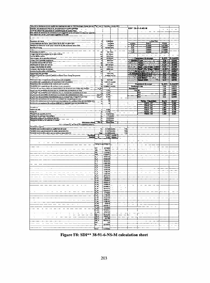
calcul do ",..~lance el do" rigid" des _"""'.- .. -So, o""""",m Deoign Manua',... ....... "" Y"""bOa" ,,_: Ml1 ,s, ,- SOI** •• e , ..
Ent~ ~ ...... des pora_ on çaractMI gras, Cee'
, ___ ,._(_ .......... t __ , ...
o ............ t .................. __ .... ,._
,"" Epa" .. ur" ,· .. ler O ... , mm Idnun'lml limll ..... "qu ••• focler , Q, ... via ,"on SOI, F, MPa p361S
,do"OClor • Q, dos .ou.u ... "'on 50', F. 31 MPa ,.,000 MPa
~ '"N,~ P,ofondeu, du Iab'.' hh 3 •. mm L.' •• ur •• , ..... (meau'" .u, le ptan 'n,II"', WV< ~." ",m Pas du tabll., (p",h, •• 102. mm oem' ..... u, do 'a _., .. 'n,.rieur. .. 19 .• ' mm L., •• u, •• , ...... , ... upOrIou .. .•. mm . "'.' ""v 'O'
,~ . ,,,.
~ ,"Omo g. 12,. lmm
~ •• racJor par 1lOMI18 SI 201.32 Imm ('"". -"., 'li Llrg.ur dos f.ulll .... tab'ler w. 'U Imm . .~
Longueur ... feuliio. do tabll" 809tI Imm
:;:i~;;' iII . Jn,
•• lNon," ••• !J np ,pout ..... 152' Imm .- ," . .;:
IMoment d·tn._ do t. _"on off.", •• on"'on , .... v • ., , 21 .... lmm'Im ~ (""W" .. ,,,·, :':.;'s. .", '~: ;"C.· IR"' ... n" ... ,"nn"teu", • ,. It""tu," (vo" d-con ... , Q, 0.41 lkN ~:':::2
1 conn"""o" i la '''oClure (,'oir ci-con,rcl 0,0312' Imm"'N I.O.,.tan, .... ,on",,--,!u", de' a, -,.31 i'" l~~illftdl'; c"nn .... "" ' ' 'ci-conlrcl 5, 1.46 IN ombre de ne"'ur<' cnlre ,,, conne"eu" • ,. "'0"0" ao, boot, d" fculll<, n_.'" Pinœmcnb ,,,''''"', ... le. pout,,'''' .'-bout <!'" w. 'n,tuant le. ,"nOK"U", .,on "".'1 "! 1,333 1>:('';-' ... t •• pou ... tto. tn'.~ .. '.,,,. ( ... w. 'n"u.n' tas ,on_".,",.n , ... ) 0, 1.33' MIO «.,Iw,' ." , .. pout .. tta. d. bout (ou, w. 'n"uant .en ,'v., «,"-,w,' o.,,. NI: 1.(.,Iw,' ou, , .. pou ... II .. , i 'w. induant , .. ,onn'''''ura.n ""0' IIx,Jw,' ..... 01' INom" .. , ,., bout ( ... w.'nd.an'''' con ...... u"' on rive, n,. INombre, ~ .'Ndura en rive (total .ur' ".,,'uan' <eux .ur poutre'le. 'n<] n, 11 l_-~
INombre , , ,outura (to,., .ur' "eoc'.anl ,eu •• ur poutrello. 'nt.: n, ,. IR."sI'"''
0.834 IFa_, 8 11.416 IR_ta"",.u panneau do bout s,. 23.'" IkNlm !R_taO<odu __ • s,. IkNlm IR_ .. O<o ..... _Io""""""'""' .. _ s,. 10.83 ,kNlm IR_ .. "", ...... SUI .. _au..- .. JO ... IkNlm
F.S. = 2."pD1K~. or 2.JO (2.7' " S01KI .... )pD1K~,
,FI.x;.,,; ... t ';.;dn, iF ............ , tde'acJor F. 0.0198 mmll<N "" F ... _ ..... . r ( ......... On, Fn 0.1431 mmll<N '''' ."""'.~., • ( ......... C F"" 0.0105 mmlkN "" FIo ....... F 0.1831 ........ N
RIgIdIfj G' 5.462 kNlmm
1 calcul .u l ,oamètr., IWY '010953 IWB .... " Ipw .161521 IMA 0,'26511
161912.6 _2 83956.28
- _3 48422.0' O.OOOI~
1 •• tE"" 1.91E"" - :_. 3.57E""
-' 1.7ge"" : .. '.06E"" '_41 34143.14 _42 196398. '_43 316208.' '-« '28521.
-" 1 .......
'-'. 52 ..... 3 _41 341'3.14 . 42 51 ..... _43 111904'
f----------- . :_41 1,191''''' :_42 '.31E"" :_" 1.93E-<l1 :_« '.3OE"" '_«1 916618 0-«, 425101. '_«3 121204' '_4« 191915' _444 3192132
DW, 2313423 - - 1-- - -OW 2 '05281. OW_3 401199 OW_' 842343. PH' 0,' On 32.0353'
1.418489
Figure F8: SDI** 38-91-6-NS-M calculation sheet
203
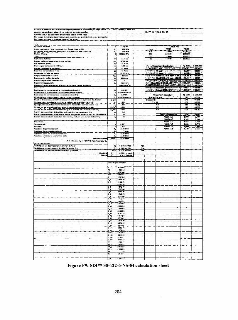
ca"", de la _tance 01 de ta """ .. d.. . "SOI O",,,,,,,,,,m Design Manual Z-".'. pa' R. T<emblay. "._2001 • SOI'" 38.i 22-6·NS·M ~ttent"', ""_ caIcuII sont 1." en SI , uOO6s • .-_
~~~~-~ ... ~~'"'!:.;... ,.,IoCOi.(HiOOlav.loui .. t • .-... ~ '-------
0 .. valo"""1, ...... _ ..... _.UfIo_ ,,'"
Opa""u, do 1'00'" 1.22 mm • (mm'/m) limlto " .. Uquo d. "00'., (pou, ,.',ut de Cl, de, vi, •• 'on SOI) F • MP, IImr '3615
.dor",10~ • Cl, dos 'oudu", •• 'on SOI) F, '" MPa O. "4000 203000 MPo O.' ~8000
r"oJ."C P,ofond .. , du tab,,,, hh 3'.1 mm 145000 La, .. u, de 1'...,. (mnu'" .u, ,. p'an 'n,"nt) - 40." mm P .. du tablle, ,plt'h) dd 152.' mm
• 'a ....,.'10 Inf.riou~ .. 1 •. 0' mm L .... u' d. 'a _110 .upOriou,. . ... mm 1- " ........ ." ' 1,"9-'6 <,' 0._', P,oject'on hori,ontolo do , • ...,. •• mm '- .. 207.32 mm
~".fl . .
L .... u' d., foui'" do Iab'io, w_ 8" mm 1·,:;· .... '" "'. Longue., de. feu"Io' de t.b'le, .... Imm INombre de, np
1 ,poutrelles 152' Imm IMoment d·'n.,t;e do '0 , , ,nea'on .ou. ,ha",. d ••• av.O) , ... .'
:n,"'·""-'''' ~.
IR .. ,.tanoo d •• ,on"",t.u,, • la ,,"'''u •• (vo', ,'-con"') a, .... IkN ;."".:?~~ . ",,'bill" d" .... nnect.un à ,.,t'u<lu,. . [ ••• ,.tan, .... ,onnK"'IS de ,outu .. ,vo', ,'-con"o) Cl. 2.3' Ik. 'COUIUr< 1./, <N} 11,1 mmt<N}
• eonn •• "'u" d, eou,"" ,voi, e1-<onl") S,
[Nomb"d. , 1 ... eonn,"" •• " à la ",.el.r. a.x bo." d,~ r •• iII .. ...pa, l'in<:etnenII [I(x,Jw) lur lei poulre'''' da bout ,Iur W. '.c'uant lei conn ..... " o. rtve) ., 1.333 Vis !118
,Iw) .u'''' , "lU' w. '.cluant'" , "Iv.) o. INIO ~,M ,,,,,,1 !",ul"lIn da_bout ('u, w. 'nc'uant le" "".) r./,<,Iw)' 0.5" ,'1' I(.,Iw)" .u, 'n po"",'''' 'nt ...... '.'". 1 t 'H ,on""'.u" .n riv.) r./,<,Iw)' •. 5" ,.14 INomb .... , 'bout, t ... , •• n_ •• oct""" ." riv.l n. 3. INomb" de 'on_"ou," • la "Notu".n rive (tota' .u. LL. ""uont 'ou •• u. pout,.. ... 'n< n. 11 TIII', ........... IN~b .. de, • ,0ulU~ (toto' .u. , •• xctuont ceu •• u' poo,,"'Io. 'nt. n. t'
IR,,,.,.,,c, O.S57
IFacteurB 11.'I.S 'd. bout 5" 23 .• 3 IkNlm , ...... _ ..
5" 11.77 IkNlm [R_ta ... _IU' 10",",,",,"",00_ 5" tO.S3 ['Nlm -IR .... tance lm"" .u ... _ du Ia_ o. ..... IkNlm
F.S .• 2.0 pou< S,. of 2.35 (2.75. 'S,
"'.x,b,",." ".,d". 'F",'biI"d ... , ,tder ...... F. 0.014: 'mmlkN 15" F .. ' ..... d ... ,ta_ (00,...... On) _ Fn _O.~ I"""",N _ -'''' 'F ... lbilltéd ... , ',panl_oC) ~ _0' ,."
FIe.IbIUté F 0.0951 mmII<N 10.513 kN"m
caIcU du, .,.,.,...,
IWT 4079953 IWB 454012 [pw 0.,.2096 IMA 0.'28571
t.'.12 .• -_2 83958.2. 3 '''22.05
0.000155
.2 ~lE~ '.91E.o
,.4 ..!5'E,<i6 "~
_5 1.'''.0 _S •. œe-08
-" 34143." _42 t98398.:
'-" 31S208.5
-" 428521. '_45 '20884 .• _4S 524895.: _41 34143." _42 516448.1
-" 'l'9042 -" 1.' .. .0
~
_42 5.37E'"
-" S.93E.o'
-" 2.35E'" '_441 9'881.
,0-é42 425'91. ~-
'_"3 J~l204l
- -- '-'" 7919,.. -- 37921' -OW. . ., ... .,
f-- OW_2 t2".'.2 OW_3 2587".' OW_' ".3.3. PH' O.,
On 20.""
3."718'
Figure F9: SDI** 38-122-6-NS-M calculation sheet
204

Des va","" de """'lanco de connodeu<s "'"'.-.... ur le alI. (selon la valeur de ,._ ~de"-",~ .. ,,,",.UIIi_.urle_
-;::;;;;----.p ..... u, de ,'"", .. "51lmm 1,(mm"/m) L1mlt ..... Uqu .... ,'''''Ie, (pou, ,alcu' de "' .... yi •• elon SOI) F. 230 IMP. R •• I"ance ulum. de r"ie, • Q, de •• ouOu .... e'on SOI) F. 310 IMpa 0.76 14000 Module O'Young 203000 IMP. 0.91 ~8000
',,"""'- 1.22 159000 p,olondeu' Ou tabll., hh ... Imm I.Sl I4SOOO ~de 1'"" ~u'" .u, ,. plan Incl)",) ww .,." Imm Pa. du IOblle, (plleh) dd 152. Imm Deml""".u, de la sem."e In"""u," .. 19." Imm lMlIeur d, 'a _,'10 .u"","u .. ... Imm ~ ~
• 1· ..... •• Imm ""<"'K ~" r ....... os 207.32 Imm I~ ;;''' ,"',
La,geu' des loulile ... labile, w. .,. Imm Longu.u, do. l.uUIo. Oe •• bll., ~, Imm
lM INomo.. de pou"'llo. Inlon"'Olal ... np 10' . ""Vi ·:b ••. • 1->0 .,.,....... ~. Imm ~ . IMomen. d·'n ....... 1. , , (1Ie.lon .ou. 'h ....... 'ay.,) , 210000 Imm"/m ,>:'<:1'-' . I~.::~· , 1-. , . '.,,,, .• ,,",,,. ~'" .' .
IR ..... ance Oe. ,onneelou," • , •• ""ctu .. (yol, cl-con ... ) '" , . ., IkN .. . ','
~·, .. Ibili" de> 'o •• ",'eu" • ,. "lUetU'" IRésl ... n" d •• c~n" ••• ". de 0. 2.37 IkN ... - _'10 1",,,1011'" d.~ ,nnn<et,"" de ,0U'Ul< ( ... Ir <I-co."') S, SouduR 16mm
~ INnmO" de ri ... 'o ...... u" à " ",uetUl< 'u< bouh d" f..,lIle'. _"J'"' lux.Jw)'u, 10. pou''''''' de bout (.u' w. Inclu.n' 1 •• eonn"'eun .n riya' ., .33: Via #8
'-
1:('.fW)'u, 1 .. pou ... IIo.lnlo= .. I.I ... (.u, w. Inclu.nt", ,onnaclou," en riv,' .. "333 1E{,jw" .u, le. po .... , ... ~(.u, w.lnc .... n .... , • riYe) 1:(x.Jw)' ..... fi; E{.Jw)' .u, 'e. poutre"" ; 1 'w. 'nelua.' les conn"tau'. en riv.) l:(x,./wl' o .... '14 Nomb .. , • de bou~1 • le. connect.u .... riva) ... 3 . Nomb" da conn.ct,un • la .1nJC1u" en riv,('ota'.u, .. ",Iuan' ceux .u, pou".11es ln •. : n. ,. T~ .... ~ ..... Nomb .. de connacteu," de coulu .. (1010' .U, 1 • ,,,Iuan' ceux .u, pou'"'''' InC n. .1.
"",so.,,"" •. 872
FacI ... B 11.476 ........... Oul"""""'" .. bouI S. 23.83 IkNlm ...... tancodu ......... u """-r. s.. 11.80 kNim Rlllistance baHe sur le connedeur de ooin s.. 10.83 kNim
R"~"nce lm'" '"' le VOIIemeIn dU""" .. 52.88 kNim m'n .. 'Q.l3 ....
F.S. '2.0"",,, S. el 2.35 (2.75;
F/."b,/,'" "'''.'''''' FIe_" 0 ... 1 'da'''''''' F. 0.0115 mnv1<N ,.% FIe_ .. Oue. ',(pa~on) Fn 0.0388 mnv1<N 61% Fie."'"0 .. 0 , Fslip 0.0132 m"""" 21%
Fie ...... F 0.0635 mm/kN RIgId .. G" 15.750 kHlmm
ICaIcU du, ... .,. •• 1
IWT 4079953 IWB ..... " IPW 0.538933
IMA 0.'28571 167912.'
_2 .3856.2.
'- -'- .~'" 0.0001"
_2 1.51'''' _3_ 7~~'"
'.57'''' 5 1.79 ....
:_6 '.06€'" . , 3414: .
'_42 196396.' "8208.'
'_44. 42852'" '_45 720884.8 .8 "'.9'.3
r---- _41 34143." _42 57844 •. ' ~ ~,
f- :_41 1.19E'" :_42. '.37E'" :_4: ..9lE'" :44 2.3SE.06 '_441 9788' >-442 425791.
'_443 1212<)4,
'_444 7919" '_444 3792132
OW 10734.02
r-- -- - OW_2 9061 OW. 188430. 1-------DW_4 208040.
PH' •.. 0-,,- 1~
' .• 33796
Figure FIO: SDI** 38-151-6-NS-M calculation sheet
205
Related Documents