University Microfilms - OhioLINK ETD Center

INFORMATION TO USERS

This dissertation was produced from a microfilm copy of the original document. While the most advanced technological means to photograph and reproduce this document have been used, the quality is heavily dependent upon the quality of the original submitted.

The following explanation of techniques is provided to help you understand markings or patterns which may appear on this reproduction.

1. The sign or "target" for pages apparently lacking from the document photographed is "Missing Page(s)". If it was possible to obtain the missing page(s) or section, they are spliced into the film along with adjacent pages. This may have necessitated cutting thru an image and duplicating adjacent pages to insure you complete continuity.

2. When an image on the film is obliterated with a large round black mark, it is an indication that the photographer suspected that the copy may have moved during exposure and thus cause a blurred image. You will find a good image of the page in the adjacent frame.

3. When a map, drawing or chart, etc., was part of the material being photographed the photographer followed a definite method in "sectioning" the material. It is customary to begin photoing at the upper left hand corner of a large sheet and to continue photoing from left to right in equal sections with a small overlap. If necessary, sectioning is continued again — beginning below the first row and continuing on until complete.

4. The majority of users indicate that the textual content is of greatest value, however, a somewhat higher quality reproduction could be made from "photographs" if essential to the understanding of the dissertation. Silver prints of "photographs" may be ordered at additional charge by writing the Order Department, giving the catalog number, title, author and specific pages you wish reproduced.

University Microfilms300 North Zeeb RoadAnn Arbor, Michigan 48T06

A Xerox Education Company

72-26,975BHAGAT, Pramode Kumar, 1944-

A MATHEMATICAL INVESTIGATION OF LEFT VENTRICULAR DISTENSIBILITY IN HEALTHY CLOSED-CHEST DOGS.The Ohio State University, Ph.D., 1972 Engineering, biomedical

University Microfilms, A XEROX Com pany, A nn Arbor, M ichigan

A MATHEMATICAL INVESTIGATION OF LEFT VENTRICULAR LISTENSIBILITYIN HEALTHY CLOSED-CHEST DOGS

DISSERTATIONPresented in Partial Fulfillment of the Requirements for

the Degree Doctor of Philosophy in the Graduate School of The Ohio State University

ByPramode Kumar Bhagat, B. Tech. (E.E.), M.S.E.E

* * * * * *

The Ohio State University 1972

T

Approved by

AdviserDepartment of Electrical Engineering

PLEASE NOTE:

S ome pa ge s m ay have indistinct print.Filmed as received.

U n i v e r s i t y M icr of i l ms , A Xero x E d ucation Comp a n y

DEDICATION

I dedicate this work to the memory of my father Basant LaL Bhagat.

ii

ACKNOWLEDGEMENTS4

It is a pleasure to acknowledge the long-term guidance and support of my advisor, Professor Herman Roscoe Weed. He introduced me to the exciting world of Bio­engineering and took special pains to teach the rudiments of engineering as applied to Physiology. Without his inspiration and constant encouragement this study might not have begun.

To Professor Russel L. Pimmel special thanks are due for his advice and encouragements in the selection of this topic and his sage counsel during the study reported here.

It is not possible to repay by words alone my deep sense of indebtedness to Professor Robert Louis Hamlin. His material assistance was exceeded only by his enthusiastic support of my academic endeavors. He served as my expert pilot through, for me, the uncharted sea of Physiology and made the whole experience a pleasure cruise.

To Dr. D. R. Gross, an excellent co-worker and friend, special thanks are due for efforts and help toward completion of the study reported here. He gave freely of his time and opened the doors of his castle of knowledge of Physiology for a free guided tour. The innumerable discussion

iii

sessions in which he participated have contributed greatly toward completion of this work. He was of great assistance with the surgical aspects reported in the study which were necessary for collection of experimental data.

Special friends deserve special thanks. To Prabhakar H. Pathak, Karaal C. Gunsagar, and Dinesh Kumar my deep gratitude for their encouragements and steadfast loyalties. Their friendship provided me with the self- assurances and motivations which were very necessary to sustain the energy required for the continuance and completion of the work of such a magnitude.

Special note of thanks are also due to the co-workers in the Biology of Heart Program. Of the numerous individuals who have assisted and encouraged me in large and small ways,X would wish to especially thank Steve Boggs for assistance with data collection, Gary Geiger for his expert technical assistance with the photographs in this study. Cathy Carter, Linda Barnett, and Linda Werner deserve special thanks for their assistance with the drawings. Margie Maxwell, who has cheerfully assisted with many details through the years, deserves my special appreciation.

Thanks are also due to Drs. Pipers, Smetzer, Gibb, Muir, and Breznock who have always been willing to share their expert knowledge. Roger Kroetz has spent many long hours of consultations during the computer simulations and he deserves my special gratitude.

iv

Friends, teachers, and professors who during my school, undergraduate and graduate studies have helped charter my quest of knowledge to present level are too numerous to detail here. I would like to thank Professor Richard H. Engelman and Professor Carl H. Osterbrock for their encouragements during my studies for the M.S.E.E. degree.To Professor V. G. K. Murthy who taught me the basics of electrical engineering when X was an undergraduate student and was my advisor during Bachelor*s degree projects, I am indebted.

In the final analysis, one owes everything both spiritual and material to his family. Throughout my formative years in school I had been very fortunate in having the wise counsel of ray parents and relatives, especially my grandfather's. My mother notwithstanding, the terrible loss that fate willed her has constantly stood by me in ray pursuit of knowledge. My older brother and his family have unselfishly provided material assistance and constant encouragement during my years of studies. My younger brothers, who decreed by their actions and willing­ness to accept family responsibilities and obligations that were partly mine and by this allowed me to continue my work, deserve special mention. To Nilu, Alolc, and Ashok, who grew up while X was away, I am sorry to have missed those years. Perhaps one day you will understand and forgive me. To all

v

of you, then, ray family I pledge to repay my debts by my deeds, as I cannot with words.

Mrs. Carolyn Shafer turned out this final typed version of the study by patient and careful attention to details and by her expertise in deciphering my writings.I am grateful to her.

Drs. Hawthorne and Fieper made available some of their experimental data for a comparative study and I thank them.

The Ohio State University Computer Center provided some free computer time during the initial phase of this study. This study was supported in part by Public Health Service Grant HL 09884 from the National Heart and Lung Institute, NIH.

vi

\

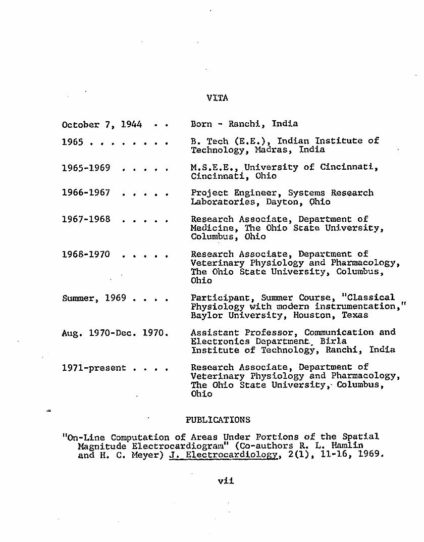
VITA

October 7, 1944 • • Born - Ranchi, India1965 . . . . . . . . B. Tech (E.E.), Indian Institute of

Technology, Madras, India1965-1969 . . . . . M.S.E.E., University of Cincinnati,

Cincinnati, Ohio1966-1967 ........ Project Engineer, Systems Research

Laboratories, Dayton, Ohio1967-1968 . . . . . Research Associate, Department of

Medicine, The Ohio State University, Columbus, Ohio

1968-1970.......... Research Associate, Department ofVeterinary Physiology and Pharmacology, The Ohio State University, Columbus,Ohio

Summer, 1969 . . . . Participant, Summer Course, "ClassicalPhysiology with modern instrumentation," Baylor University, Houston, Texas

Aug. 1970-Dec. 1970. Assistant Professor, Communication andElectronics Department.. Birla Institute of Technology, Ranchi, India

1971-present . . . . Research Associate, Department ofVeterinary Physiology and Pharmacology, The Ohio State University,' Columbus,Ohio

PUBLICATIONS"On-Line Computation of Areas Under Portions of the Spatial

Magnitude Electrocardiogram" (Co-authors R. L. Hamlin and H. C. Meyer) J. Electrocardiology, 2(1), 11-16, 1969.

"A Method for Teaching Genesis of the Electrocardiogram and Simulating Effects of Morphologic and Conduction Defects" (co-authors R. L. Hamlin and C. R. Smith). Am. J. Vet. Res., 31(12), 2289-2300, 1970.

"Model of Urine Flow Regulation" (co-authors T. G. Cleaver, L, Mace, W. H. Pierce, R. Gruenke, and H. R. Weed).Third Southeastern SymposS.um on System Theory, Atlanta, Georgia, 1971.

FIELDS OF STUDYMajor Field: Electrical Engineering

Studies in Control Theory. Professor F. C. WeimerStudies in Computer Theory. Professor R. B. LackeyStudies in Network Analysis and Synthesis. Professor

W. DavisStudies In Quantum Mechanics. Professor H. J. Hausman Studies in Bio Medical Engineering. Professor H. R. Weed Studies in Physiology. Professor R. L. Hamlin

viii

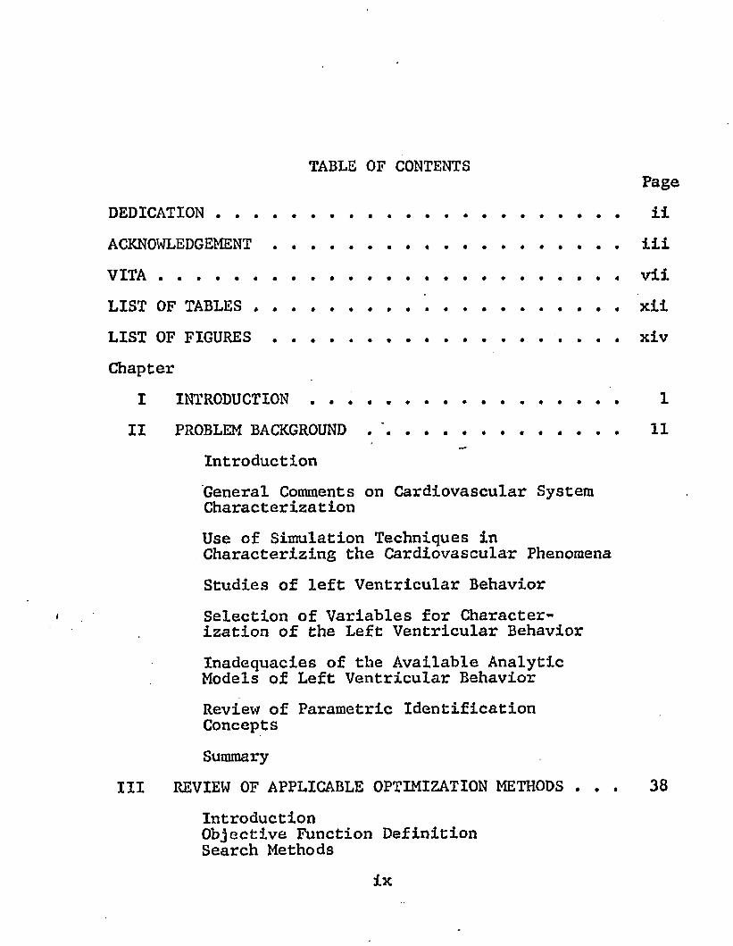
TABLE OF CONTENTSPage

DEDICATION........................................... iiACKNOWLEDGEMENT ..................................... illV I T A ....................................................viiLIST OF TABLES............ .......................... xiiLIST OF F I G U R E S .............................. xivChapter

I INTRODUCTION . . . . . . . ..................... 1II PROBLEM BACKGROUND . '............ 11

IntroductionGeneral Comments on Cardiovascular System CharacterizationUse of Simulation Techniques in Characterizing the Cardiovascular PhenomenaStudies of left Ventricular BehaviorSelection of Variables for Character­ization of the Left Ventricular BehaviorInadequacies of the Available Analytic Models of Left Ventricular BehaviorReview of Parametric Identification ConceptsSummary

III REVIEW OF APPLICABLE OPTIMIZATION METHODS . . . 38IntroductionObjective Function Definition Search Methods

ix

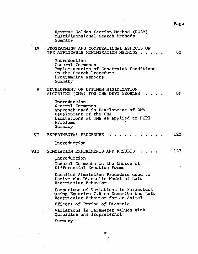
PageReverse Golden Section Method (RGSM) Multidimensional Search Methods Summary

IV PROGRAMMING AND COMPUTATIONAL ASPECTS OFTHE APPLICABLE MINIMIZATION METHODS........ 60

Introduction General CommentsImplementation of Constraint Conditions in the Search Procedure Programming Aspects Summary

V DEVELOPMENT OF OPTIMUM MINIMIZATIONALGORITHM (OMA) FOR THE DEPI PROBLEM . . . . 89

Introduction General CommentsApproach used in Development of OMADevelopment of the OMALimitations of OMA as Applied to DEPIProblemsSummary

VI EXPERIMENTAL PROCEDURE...................... 122Introduction

VII SIMULATION EXPERIMENTS AND R E S U L T S ......... 127IntroductionGeneral Comments on the Choice of Differential Equation FormsDetailed Simulation Procedure used to Derive the Diastolic Model of Left Ventricular BehaviorComparison of Variations in Parameters using Equation 7.6 to Describe the Left Ventricular Behavior for an AnimalEffects of Period of DiastoleVariations in Parameter Values with Quinidine and IsopreternolSummary

x

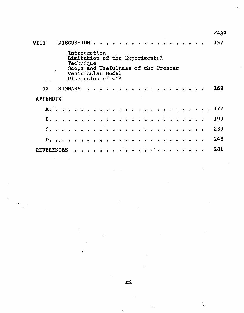
VIII DISCUSSIONPage157

IntroductionLimitation of the Experimental TechniqueScope and Usefulness of the Present Ventricular Model Discussion of OMA

IX SUMMARY . ................................... 169APPENDIX

A . ................ 172B .............. 199C.................. 239D. ...................... 248

REFERENCES............... - ............... 281

xi

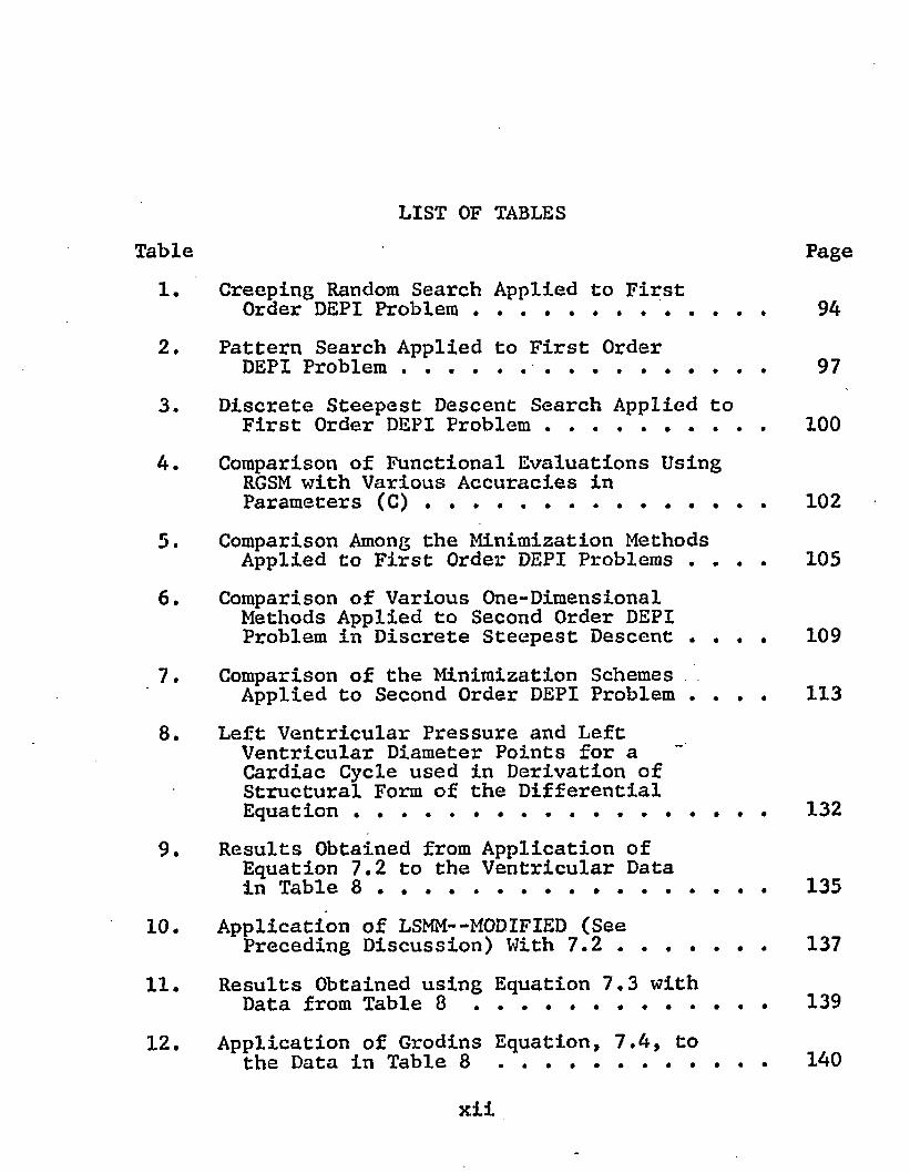
LIST OF TABLESTable Page

1. Creeping Random Search Applied to FirstOrder DEPI Problem......................... 94

2. Pattern Search Applied to First OrderDEPI Problem............ 97

3. Discrete Steepest Descent Search Applied toFirst Order DEPI Problem................... 100

4. Comparison of Functional Evaluations UsingRGSM with Various Accuracies inParameters ( C ) ............................. 102

5. Comparison Among the Minimization MethodsApplied to First Order DEPI Problems . . . . 105

6. Comparison of Various One-DimensionalMethods Applied to Second Order DEPIProblem in Discrete Steepest Descent . . . . 109

7. Comparison of the Minimization SchemesApplied to Second Order DEPI Problem . . . . 113

8. Left Ventricular Pressure and LeftVentricular Diameter Points for aCardiac Cycle used in Derivation ofStructural Form of the DifferentialEquation ......................... . . . . . 132

9. Results Obtained from Application ofEquation 7.2 to the Ventricular Datain Table 8 ................................. 135

10. Application of LSMM--MODIFIED (SeePreceding Discussion) With 7 . 2 ............ 137

11. Results Obtained using Equation 7.3 withData from Table 8 139

12. Application of Grodins Equation, 7.4, tothe Data in Table 8 .............. 140

xii

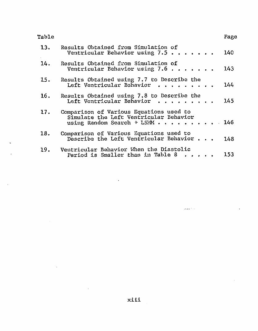
Table Page13. Results Obtained from Simulation of

Ventricular Behavior using 7.5 ............ 14014. Results Obtained from Simulation of

Ventricular Behavior using 7.6 ............ 14315. Results Obtained using 7.7 to Describe the

Left Ventricular Behavior . . . . . . . . . 14416. Results Obtained using 7.8 to Describe the

Left Ventricular Behavior ................ 14517. Comparison of Various Equations used to

Simulate the Left Ventric;ular Behaviorusing Random Search + L S M M ................ 146

18. Comparison of Various Equations used toDescribe the Left Ventricular Behavior . . . 148

19. Ventricular Behavior When the DiastolicPeriod is Smaller than ixi Table 8 . . . . . 153

xiii

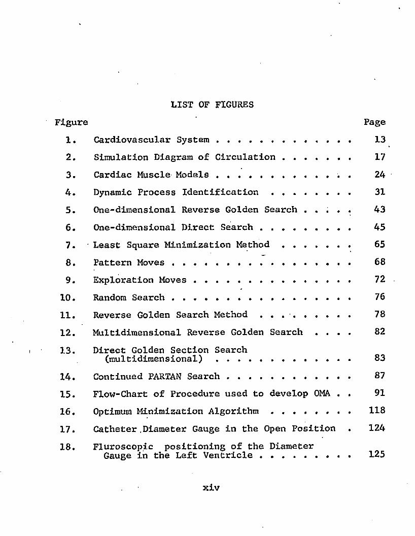
LIST OF FIGURESFigure Page

1. Cardiovascular System .......................... 132. Simulation Diagram of Circulation........... . 173. Cardiac Muscle Models . ......... . . . . . . . 244. Dynamic Process Identification ............... 315. One-dimensional Reverse Golden Search . . . . . 436. One-dimensional Direct Search ................. 457. • Least Square Minimization M e t h o d ............. 658. Pattern M o v e s .................................. 689. Exploration M o v e s .............................. 72

10. Random Search.................................. 7611. Reverse Golden Search Method ........... 7812. Multidimensional Reverse Golden Search . . . . 8213. Direct Golden Section Search(multidimensional) ......................... 8314. Continued PARTAN Search ........................ 8715. Flow-Chart of Procedure used to develop OMA . . 9116. Optimum Minimization A l g o r i t h m ............... 11817. Catheter.Diameter Gauge in the Open Position . 12418. Fluroscopic positioning of the Diameter

Gauge in the Left Ventricle................. 125

xiv

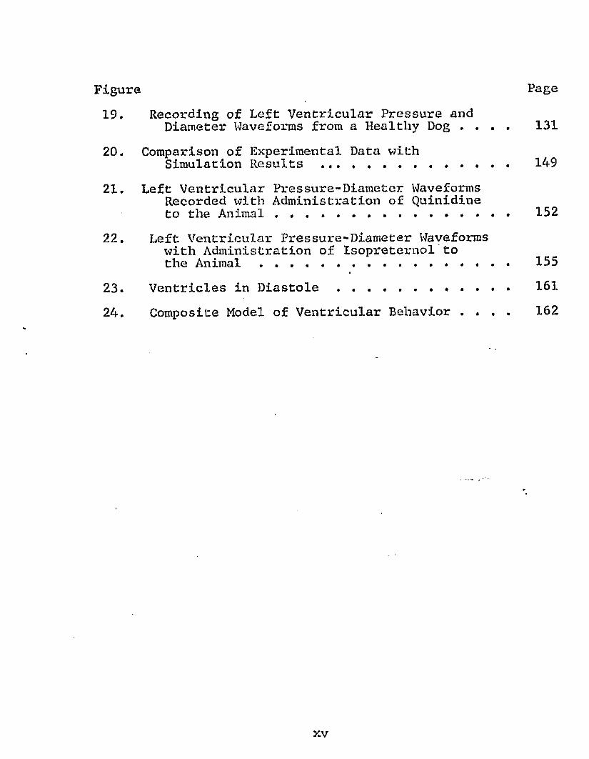
Figure Page19. Recording of Left Ventricular Pressure and

Diameter Waveforms from a Healthy Dog . . . . 13120. Comparison of Experimental Data with

Simulation Results ......................... 14921. Left Ventricular Pressure-Diameter Waveforms

Recorded with Administration of Quinidineto the Animal ............................. 152

22. Left Ventricular Pressure-Diameter Waveformswith Administration of Isopreternol tothe A n i m a l ................................. 155

23. Ventricles in Diastole ............. . . . . . 16124. Composite Model of Ventricular Behavior . . . . 162

xv

CHAPTER I INTRODUCTION

The ventricles of a mammal are responsible for the circulation of blood throughout the animal*s body. Atevery heart beat the energy required to drive blood throughthe circulatory system is derived from inherent contractile mechanisms of the muscle tissues. A heart beat consists of two phases:

1. Diastolic, or relaxation phase2. Systolic, or contraction phaseDuring diastole the ventricles fill with blood due

to a higher pressure in the atria. During systole the ventricles eject a portion of the blood Into the circulation. Previous characterizations of the ventricular behavior have been concerned mainly with the systolic phase and its characteristics during diastole have not been investigated in detail. It is felt that because of this approach many questions regarding the effects of physiological changes on cardiac function, in general, have remained unanswered.It is hoped that a complete characterization of the diastolic behavior may provide insight into the behavior of ventricular muscle in health and/or disease.

1

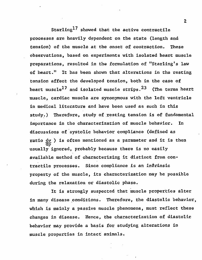
S t a r l i n g ^ - ? showed that: the active contractileprocesses are heavily dependent on the state (length andtension) of the muscle at the onset of contraction. Theseobservations, based on experiments with isolated heart musclepreparations, resulted in the formulation of "Starling's lawof heart." It has been shown that alterations in the restingtension affect the developed tension, both in the case ofheart muscle^ and isolated muscle strips.^ (The terms heartmuscle, cardiac muscle are synonymous with the left ventriclein medical literature and have been used as such in thisstudy.) Therefore, study of resting tension is of fundamentalimportance in the characterization of muscle behavior. Indiscussions of systolic behavior compliance (defined asratio dv ) is often mentioned as a parameter and it is then Hpusually ignored, probably because there is no easily available method of characterizing it distinct from con­tractile processes. Since compliance is an intrinsic property of the muscle, its characterization may be possible during the relaxation or diastolic phase.

It is strongly suspected that muscle properties alter In many disease conditions. Therefore, the diastolic behavior, which is mainly a passive muscle phenomena, must reflect these changes in disease. Hence, the characterization of diastolic behavior may provide a basis for studying alterations in muscle properties in intact animals.

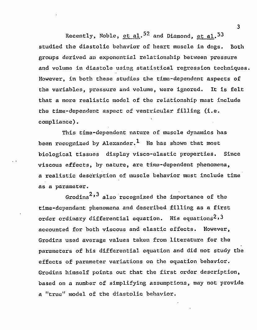
3Recently, Noble, et al.^2 and Diamond, et al.^3

studied the diastolic behavior of heart muscle in dogs. Both groups derived an exponential relationship between pressure and volume in diastole using statistical regression techniques However, in both these studies the time-dependent aspects of the variables, pressure and volume, were ignored. It is felt that a more realistic model of the relationship must include the time-dependent aspect of ventricular filling (i.e. compliance).

This time-dependent nature of muscle dynamics has been recognized by Alexander.^ He has shown that most biological tissues display visco-elastic properties. Since viscous effects, by nature, are time-dependent phenomena, a realistic description of muscle behavior must include time as a parameter.

2 3Grodins * also recognized the importance of the time-dependent phenomena and described filling as a first order ordinary differential equation. His equations^>3 accounted for both viscous and elastic effects. However, Grodins used average values taken from literature for the parameters of his differential equation and did not study the effects of parameter variations on the equation behavior. Grodins himself points out that the first order description, based on a number of simplifying assumptions, may not provide a "true" model of the diastolic behavior.

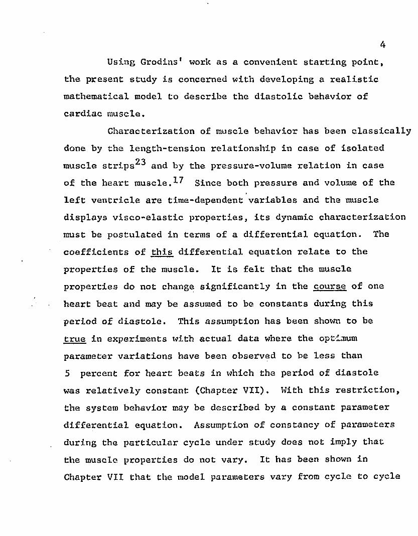
4Using Grodins1 work as a convenient starting point,

the present study is concerned with developing a realistic mathematical model to describe the diastolic behavior of cardiac muscle.

Characterization of muscle behavior has been classicallydone by the length-tension relationship in case of isolated

2 muscle strips and by the pressure-volume relation in case of the heart m u s c l e . Since both pressure and volume of the left ventricle are time-dependent variables and the muscle displays visco-elastic properties, its dynamic characterization must be postulated in terms of a differential equation. The coefficients of this differential equation relate to the properties of the muscle. It is felt that the muscle properties do not change significantly in the course of one heart beat and may be assumed to be constants during this period of diastole. This assumption has been shown to be true in experiments with actual data where the optimum parameter variations have been observed to be less than 5 percent for heart beats in which the period of diastole was relatively constant (Chapter VII). With this restriction, the system behavior may be described by a constant parameter differential equation. Assumption of constancy of parameters during the particular cycle under study does not imply that the muscle properties do not vary. It has been shown in Chapter VII that the model parameters vary from cycle to cycle

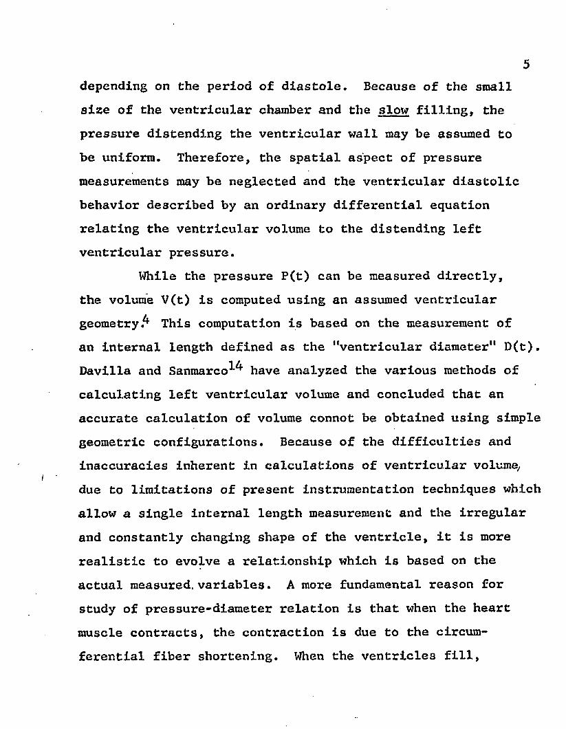
depending on the period of diastole. Because of the small size of the ventricular chamber and the slow filling, the pressure distending the ventricular wall may be assumed to be uniform. Therefore, the spatial aspect of pressure measurements may be neglected and the ventricular diastolic behavior described by an ordinary differential equation relating the ventricular volume to the distending left ventricular pressure.

While the pressure P(t) can be measured directly, the volume V(t) is computed using an assumed ventricular geometry/* This computation is based on the measurement of an internal length defined as the "ventricular diameter" D(t). Davilla and Sanmarco^ have analyzed the various methods of calculating left ventricular volume and concluded that an accurate calculation of volume connot be obtained using simple geometric configurations. Because of the difficulties and inaccuracies inherent in calculations of ventricular volume, due to limitations of present instrumentation techniques which allow a single internal length measurement and the irregular and constantly changing shape of the ventricle, it is more realistic to evolve a relationship which is based on the actual measured, variables. A more fundamental reason for study of pressure-diameter relation is that when the heart muscle contracts, the contraction is due to the circum­ferential fiber shortening. When the ventricles fill,

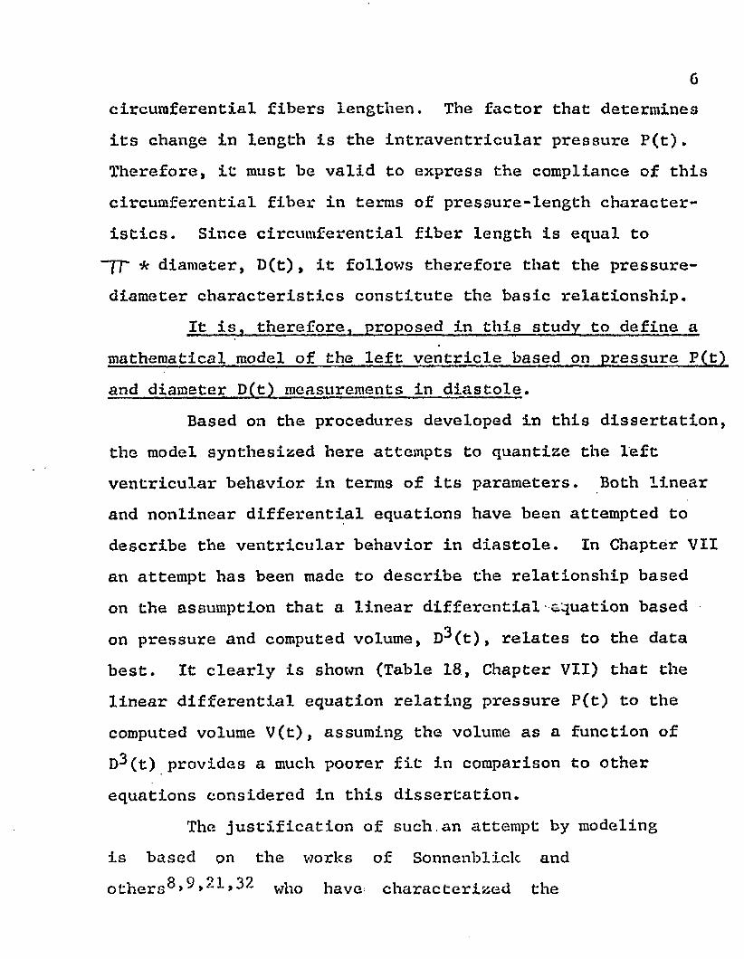
circumferential fibers lengthen. The factor that determines its change in length is the intraventricular pressure P(t). Therefore, it must be valid to express the compliance of this circumferential fiber in terms of pressure-length character­istics. Since circumferential fiber length is equal to

”77' * diameter, D(t), it follows therefore that the pressure- diameter characteristics constitute the basic relationship.

It is. therefore, proposed in this study to define a mathematical model of the left ventricle based on pressure P(t) and diameter D(t) measurements in diastole.

Based on the procedures developed in this dissertation, the model synthesized here attempts to quantize the left ventricular behavior in terms of its parameters. Both linear and nonlinear differential equations have been attempted to describe the ventricular behavior in diastole. In Chapter VII an attempt has been made to describe the relationship based on the assumption that a linear differential aquation based on pressure and computed volume, D^(t), relates to the data best. It clearly Is shown (Table 18, Chapter VII) that the linear differential equation relating pressure P(t) to the computed volume V(t), assuming the volume as a function of D^(t) provides a much poorer fit in comparison to other equations considered in this dissertation.

The justification of such.an attempt by modeling is based on the works of Sonnenblick and others^ >21,32 wj10 have characterized the

systolic behavior of cardiac muscle In terms of parametric mechanical models. In such models springs are used to simulate the elastic properties of the muscle and the contractile properties are represented by measured force- velocity relationship.

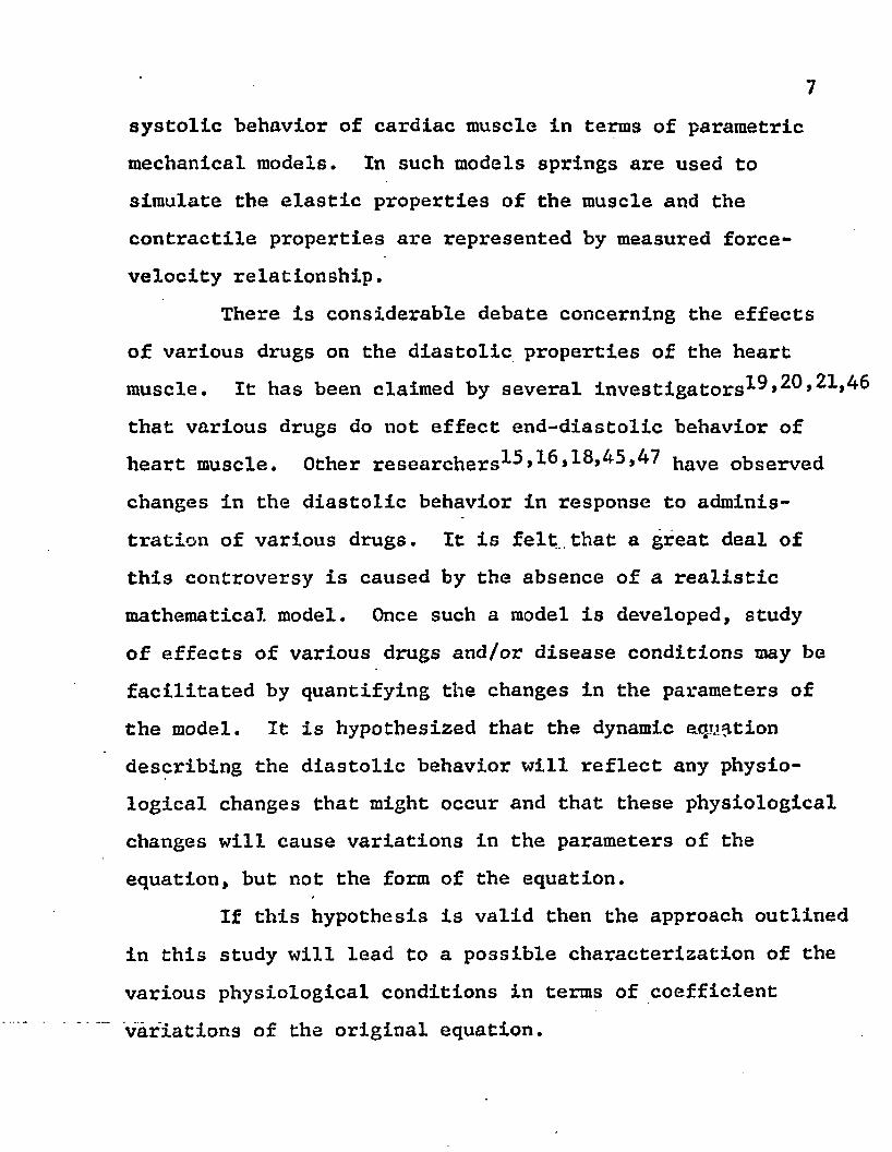
There is considerable debate concerning the effects of various drugs on the diastolic properties of the heart muscle. It has been claimed by several i n v e s t i g a t o r s ^ >21,46 that various drugs do not effect end-diastolic behavior of heart muscle. Other researchers-*'-*>16,18,45,47 have observed changes In the diastolic behavior in response to adminis­tration of various drugs. It is felt that a great deal of this controversy is caused by the absence of a realistic mathematical model. Once such a model is developed, study of effects of various drugs and/or disease conditions may be facilitated by quantifying the changes in the parameters of the model. It is hypothesized that the dynamic aquation describing the diastolic behavior will reflect any physio­logical changes that might occur and that these physiological changes will cause variations in the parameters of the equation, but not the form of the equation.

If this hypothesis is valid then the approach outlined in this study will lead to a possible characterization of the various physiological conditions in terms of coefficient variations of the original equation.

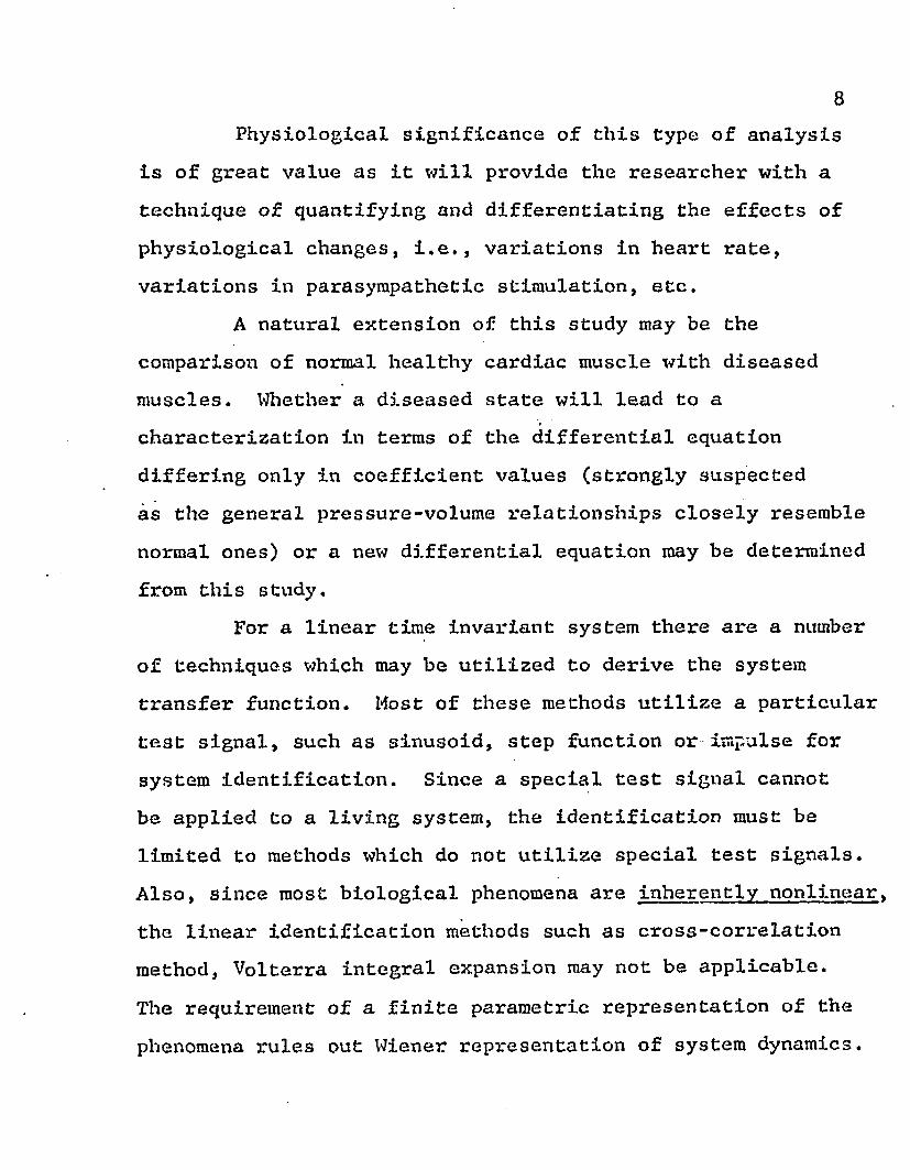
8Physiological significance of this type of analysis

is of great value as it will provide the researcher with a technique of quantifying and differentiating the effects of physiological changes, i.e., variations in heart rate, variations in parasympathetic stimulation, etc.

A natural extension of this study may be the comparison of normal healthy cardiac muscle with diseased muscles. Whether a diseased state will lead to a characterization in terras of the differential equation differing only in coefficient values (strongly suspected as the general pressure-volume relationships closely resemble normal ones) or a new differential equation may be determined from this study.

For a linear time invariant system there are a number of techniques which may be utilized to derive the system transfer function. Most of these methods utilize a particular test signal, such as sinusoid, step function or impulse for system identification. Since a special test signal cannot be applied to a living system, the identification must be limited to methods which do not utilize special test signals. Also, since most biological phenomena are inherently nonlinear, the linear identification methods such as cross-correlation method, Volterra integral expansion may not be applicable.The requirement of a finite parametric representation of the phenomena rules out Wiener representation of system dynamics.

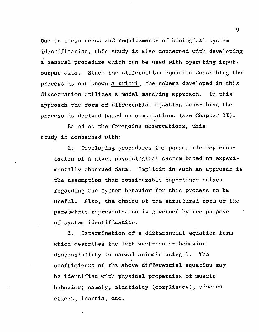
9Due to these needs and requirements of biological system identification, this study is also concerned with developing a general procedure which can be used with operating input- output data. Since the differential equation describing the process is not known a priori, the scheme developed in this dissertation utilizes a model matching approach. In this approach the form of differential equation describing the process is derived based on computations (see Chapter IX).

Based on the foregoing observations, this study is concerned with:

1. Developing procedures for parametric represen­tation of a given physiological system based on experi­mentally observed data. Implicit in such an approach is the assumption that considerable experience exists regarding the system behavior for this process to be useful. Also, the choice of the structural form of the parametric representation is governed by "me purposeof system identification.

2. Determination of a differential equation form which describes the left ventricular behavior distensibility in normal animals using 1. The coefficients of the above differential equation may be identified with physical properties of muscle behavior; namely, elasticity (compliance), viscous effect, inertia, etc.

103. Testing the differential equation form developed

in 2 with data obtained under various physiological conditions (induced by administration of different drugs) and quantifying the changes in coefficient values due to these drugs.

CHAPTER IX

PROBLEM BACKGROUND

IntroductionThis chapter begins with a brief introduction of the

cardiovascular phenomena and its characterization. The difficulties of deriving analytic expressions relating cardiovascular variables and the need to formulate the system description in terms of input-output variables are discussed.

General Comments on Cardio­vascular System Characterization

The function of the heart is maintenance of blood circulation. During the 17th Century Harvey,^2 universally recognized as the father of modern cardiovascular physiology, extensively studied the phenomena of heart action especially as it related to the movement of blood in the body. Harvey’s observations established the existence of a closed loop circulatory system for the flow of blood.

In the early 19th Century it was discovered that the normal functioning of the heart and circulation depended to a great extent on neural activity.? In this period many nerves which affected circulation were discovered and the works of

11

12E. H. and E. F. Weber, Claude Bernard, Ludwig, etc. played the central role in this phase of work. These workers provided an insight to the possible modifying actions of neuro-humoral inputs on heart behavior.

Based on the early observations of Harvey, followed by the workers concerned with the nervous activity on the heart, the study of the cardiovascular system evolved into

7two distinct phases:1. Study of the neuro-humoral phenomena which govern

and regulate the behavior of the circulatory system.2. Study of the circulatory system with neuro-

humoral inputs excluded.There have been several attempts^,3,7,12,24,25,35,

36,50,51 macie to mathematically characterize the dynamics of the circulatory system--most notable among them is the work of Grodins.^*^ In order to mathematically characterize the circulatory system, the following three variables must be experimentally evaluated:

1. Volumes of the various chambers2. Blood flow3. Pressures at various pointsEach of the above parameters is interdependent and

a complex and possibly nonlinear function of time, neuro- humoral state and their location within the system. Other variable factors, including homeostatic phenomena, complicate these relationships.

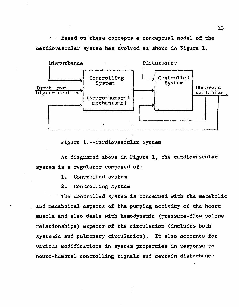
13Based on these concepts a conceptual model of the

cardiovascular system has evolved as shown in Figure 1.

Disturbance Disturbance

Controlling 1 > ControlledSystem System

Input from . Observedhigher centers variables *

(Neuro-humoralmechanisms)

Figure 1.— Cardiovascular System

As diagramed above in Figure 1, the cardiovascular system is a regulator composed of:

1. Controlled system2. Controlling systemThe controlled system is concerned with the metabolic

and mecahnical aspects of the pumping activity of the heart muscle and also deals with hemodynamic (pressure-flow-volume relationships) aspects of the circulation (includes both systemic and pulmonary circulation), It also accounts for various modifications in system properties in response to neuro-humoral controlling signals and certain disturbance

14Inputs (i.e. local changes in system properties) which may be introduced at any point into the system.

The "controlling system" deals with various phenomena, both neural and/or humoral in nature, which modify and regulate the behavior of the controlled system, based on information from the observed variables (ex. CNS ischemic feedback, heart rate control, etc.). In addition to the signals that the controlling system obtains concerning the variables of the controlled system, there are other command inputs to the controlling system from the higher centers based on body requirements. The controlling system processes these command inputs in order to generate regulatory commands for the controlled system so that body requirements may be satisfied.

Use of Simulation Techniques in Characterizing the Cardiovascular Phenomelna

Because of the complexities involved in describing actual details of the controlled and controlling systems, simulation techniques have been used. These techniques allow one to explain heart behavior in terms of well-defined physical phenomena. Use of simulation techniques in physiological phenomena is justified on the following basis:

1. Ease of deriving cause-effect relations based on the experimental data. This approach is further justifiable in physiological simulations, since in most

cases the actual phenomena are not well understood.Many times the analytic expressions are too complex to provide a physically realizable model of a physiological event. For example, in the case of the heart, because of the irregular ventricular shape, an accurate analytic expression for the determination of volume is very difficult to derive. However, there are certain problems connected with this approach. Since the simulation model is based on the actual input signal, which may be an arbitrary function of time and no special test signals can be introduced to the actual system, the identification is non-unique in general. There is also the possibility of erroneous results from the simulation model used with different input signals if the process is nonlinear.Since the biological processes are generally nonlinear, the derivation of simulation models must, therefore be limited to actual operating signals. Limited assurances of uniqueness of the model may be obtained by repeating the simulation with several sets of input-output data.

2. Simulations allow the parameters of the model to be varied with ease. Thus, various known physiological conditions may be simulated using a model. This feature enables one to study either the genesis of a particular physiologic event or the alteration of a given physiologic or disease condition by variations of parameters of the model.

163. Once a sufficiently accurate physiologic

simulation model is available, various physiological and/or pathological conditions can often be studied in a shorter period of time and at lower cost than with traditional experimental techniques. Simulation experiments also allow the time scaling of the process under study. A rapidly occuring physiological phenomena may be simulated with a greatly expanded time scaling permitting an insight into the process. Also disease conditions, which may require a large amount of time to develop in actual experiments,can be simulated with a significant reduction in time for its genesis.

4. A simulation model provides for an accurate control of the variations in parameters of the system.Thus, effects of changes in one or more parameters, independent of the rest of the system, can be studied with .ease. ~

5. Finally, a simulation model may provide a better understanding of the physiological phenomena under study.

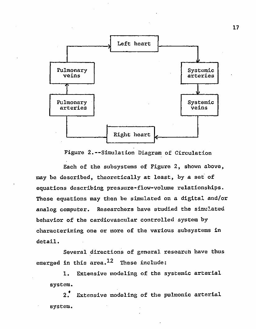
In order to utilize simulation techniques in cardiovascular system study, the controlled system (heart and circulation) is replaced by a schematic information flow diagram as shown in Figure 2. The arrows point in the direction of normal blood flow.

Left heart

Right heart

Systemicveins

Systemicarteries

Pulmonaryveins

Pulmonaryarteries

Figure 2.— Simulation Diagram of Circulation

Each of the subsystems of Figure 2, shown above, may be described, theoretically at least, by a set of equations describing pressure-flow-volume relationships. These equations may then be simulated on a digital and/or analog computer. Researchers have studied the simulated behavior of the cardiovascular controlled system by characterizing one or more of the various subsystems in detail.

Several directions of general research have thus emerged in this area.^ These include:

1. Extensive modeling of the systemic arterial system.

2.* Extensive modeling of the pulmonic arterial system.

3. Modeling of the venous system.4. Modeling the heart action.Modeling of the arterial system (mainly systemic)

has a long history dating back to Frank (1895).^ Frank was concerned with providing a biophysical description of the systemic arterial pressure and flow pulse. This area of cardiovascular research was aided, to a great extent, by the availability of comparable hydrodynamic theory. As stated by Grodins and Buoncristiani:^ "It was only necessary to solve the nonlinear partial differential equations of Navier-Stokes for three dimensional flow of viscous fluid in a complex network of elastic vessels!" Due to the complexity of obtaining an analytic solution of the above, Frank devised his famous "windkessel" theory, while others in recent years formulated the problem directly in terms of passive electrical networks. Most notably, Noordergraff, et al.^4 constructed an electrical analog of the systemic arterial tree composed of 113 segments. Each segment of this tree contained resistive, inductive and capacitive (RLC) components. The values of these components were derived from actual pressure- flow studies in systemic arterial vessels.

Until recently the pulmonic arterial system was largely neglected and it was generally assumed that the pulmonary pressure-flow relationships were similar to that of the systemic circulation. Wiener, et al. ^ studied the

19pulmonary circulation based on branching of elastic tubes.Wiener's model is more realistic since it differs from the

9 6previous models^" which characterized the circulation as terminating in a lumped impedence.

There have been very few studies relating to the simulation of the venous system. Part of the problem is due to lack of a comparable hydro-dynamic theory for flow of non-newtonian fluids in totally collapsible tubes. This is presently an area of active research37,39,49 and attempts are being made to derive pressure-flow relations based, on experimental data.^

Studies of Left Ventricular Behavior

In spite of the importance of the heart muscle in thecirculatory system, there have been very few attempts to modelits action. The study of heart action may be traced to theworks of Frank^ and Starling.^ These workers investigatedthe functioning of isolated heart which led to the formulationof "Starling's law of heart."

While Starling-^ himself appreciated the fact thatthe functioning of the isolated heart could be substantiallyaltered by nervous/humoral mechanisms and made reference tothis fact, other investigators in this period of time(1920 to 1943) largely ignored the neuro-humoral effects.These workers oversimplified "Starling's law of the heart" to

20

read: "Cardiac output is determined by venous return."27Rushmer has demonstrated that this simplified statement

cannot adequately describe behavior of intact heart.The earliest model of heart action reported in the

literature is that of Van Harreveld and Shadle.^® These workers developed a mechanical model of circulation. In this model the heart action was described by a hydraulic pump and the oversimplified Starling's law was implicitly assumed.

While this pump simulated the maximum flow and/orpressure, there was little attempt to describe the ventriculardynamics. This neglect of ventricular dynamics was prevalentin the early simulation of cardiovascular system and to quoteGrodins^: "Some models appeared which did consider ventriculardynamics, but only in terms of highly contrived time-varyingcompliances without real reference to basic myocardialproperties." In others the heart action was simulated usinga clipped voltage wave form and a sinusiodal forcing inseries with a fixed compliance.29,30,34

2 3Grodins * used control system concepts to define an isolated ventricle. He separated the two phases of the cardiac cycle, systole and diastole, in order to arrive at a transfer function relating pressure and volume of the isolated ventricle. Grodins^described filling as a first order

21

linear process and notes that the equation cited below is adequate for study of steady state behavior of circulation:

(2.1) RC Vd + Vd - C Pv

Where:Vd “ volume of ventricle in diastole Vd ** rate of blood flow Pv - venous filling pressure R ■ total viscous resistance to filling C *■ compliance of the relaxed ventricle

For the simulation Grodins used experimentally derived average values for R and C taken from the literature.

oGrodins^ notes that the incorporation of various modifications to account for the initial phase of diastole, where intraventricular pressure decreases with time contributed very little to the overall performance of the cardiovascular system.

With the studies of Sonnenblick and o t h e r s ® * ^ *21*32 in modeling length-tension relationships of isolated papillary muscles, the recent trend in cardiovascular simulations has been towards characterization of ventricular behavior in terms of a mechanical model.

cAlong these lines RobinsonJ characterized the isolated left ventricle in terras of a two-element cardiac muscle model. The cardiac muscle (ventricle in this case) is represented by a series element (S.E.), characterized by a

22

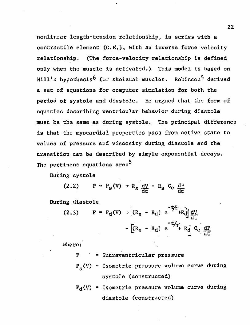
nonlinear length-tension relationship, in series with acontractile element (C.E.), with an inverse force velocityrelationship. (The force-velocity relationship is definedonly when the muscle is activated.) This model is based onHill^ hypothesis^ for skeletal muscles. Robinson^ deriveda set of equations for computer simulation for both theperiod of systole and diastole. He argued that the form ofequation describing ventricular behavior during diastolemust be the same as during systole. The principal differenceis that the myocardial properties pass from active state tovalues of pressure and viscosity during diastole and thetransition can be described by simple exponential decays.

5The pertinent equations are:During systole

P “ Intraventricular pressure Pc00 ™ Isometric pressure volume curve during

systole (constructed) pd W “ Isometric pressure volume curve during

diastole (constructed)

(2.2) P - P8(V) + Rs dV - Rs Ce dPat dtDuring diastole

'+ M ce 4E

where:

23V “ Total volume of the ventricleRs “ Coefficient of myocardial viscosity during

systoleR^ * Coefficient of myocardial viscosity during

diastole" Relaxation time constant of the myocardium viscosity

Ce ■ Compliance of that portion of theventricular volume contributed by the stretching of series elastic component of myocardium.

The above derivations were based on transformation from length-tension relationships in the muscle to the ventricular dynamics assuming a thin-walled vessel (Laplace's law) and a cylinderical shape of the vessel.

Grodins and Buoncristiani^ defined a conceptual model for a digital computer simulation of ventricular behavior during the phases of isometric relaxation, filling, isometric contraction and ejection. In this simulation^ Robinson's model of ventricular behavior was implicitly assumed.

However, according to Brady,® the two-element model is generally invalid for cardiac muscle due to the existence of a significant diastolic force. This consideration requires that the model of heart muscle must consist of at least three functionally distinct elements. Two such models have

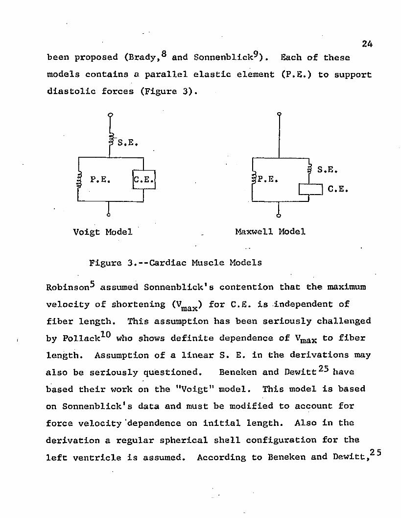
been proposed (Brady,® and Sonnenblick^). Each of these models contains a parallel elastic element (P.E.) to support diastolic forces (Figure 3).

S.E

C.E.P.E.

Voigt Model

P.E.S.E.“ C.E.

IMaxwell Model

Figure 3.--Cardiac Muscle Models

Robinson** assumed Sonnenblick1s contention that the maximum velocity of shortening (Vraax) for C.E. is independent of fiber length. This assumption has been seriously challenged by Pollack^® who shows definite dependence of to fiberlength. Assumption of a linear S. E. in the derivations may also be seriously questioned. Beneken and Dewitt 5 have based their work on the "Voigt” model. This model is based on Sonnenblick's data and must be modified to account for force velocity dependence on initial length. Also in the derivation a regular spherical shell configuration for theleft ventricle is assumed. According to Beneken and Dewitt,25

25

in the normal operating range, the maximum and minimum pressure-volume relationship are more or less linear and may be described by:

(2.A) P » a(t) * (V - Vu ) where:

P ventricular pressureV ■ total ventricular volumea(t) *■ time dependent elastance which is small

in diastole and large in systole Vu ** represents the unstressed ventricular

volume.It is noted that in almost all the studies concerned

with muscle models very little attempt has been made tocharacterize the muscle in its relaxing state. This neglectmay be attributed, in part, to Hill's pioneering work on skeletal muscle.^ Hill was mainly interested in the contractile mechanism of the skeletal muscle and defined relaxation as the "process by which the muscle returns, after contraction, to its initial length or tension."H>38 Characterization of the relaxation phase was not considered important in defining muscle behavior by researchers who applied Hill's concepts to cardiac muscle.

While relegation of muscle relaxation properties to secondary importance may be quite valid when dealing with

26isolated muscle preparations, they must not be ignored in a dynamic study involving periodic contraction and relaxation!A definite need exists for understanding the cardiac muscle behavior, since the circulatory response to physiological changes is governed by modifications of cardiac contractile activity. The study of the diastolic phase of the cardiac cycle is of great importance, since it is important in modification of the contractile mechanism.

Noble, et al.^2 and Diamond, et al.^3 have attempted to characterize the diastolic pressure-volume relationship by an exponential equation:

<2-5> § - a + bFwhere:

dP a 1Hv compliancea, b « constantsP » diastolic left ventricular pressure

Two serious objections may be raised in regard to theequation cited above.

1. The time dependent aspects of the ventricular phenomena are ignored. But in a dynamic study of a periodic event (cardiac cycle) the time variations of both pressure and volume must be considered of primary importance.

272. The volume used in the derivation of the above

equation has been computed using a simple geometry described by analytical expression. This approach is not very accurate from the standpoint of deriving a diagnostic criteria since the ventricles, in reality, have an irregular shape varying with time.

It can be seen from the foregoing discussion that the Grodins^ and Noble models^ of ventricular diastole fall short of the ideal. Since the ideal model will enable one to predict changes in muscle properties, one must search for a logical method of obtaining these ends. Therefore, the study was initiated with the stated aim of an attempt to mathematically describe the diastolic behavior of the left ventricle.

Selection of Variables for Characterization of the Left Ventricular Behavior

The left ventricle represents a hollow viscoelastic cavity in which the distension of the walls is caused by the pressure exerted due to the existing mass of blood. A description of its behavior is normally given in terms of pressure F(t) and computed volume V(t) measurements. This description leads to the definitions of ventricular behavior in terms of compliance (rate of change of pressure with volume or diameter) and viscous effects. This approach has

28o obeen used by Grodins who related pressure to the computed volume in terms of a first order differential equation as stated earlier in this chapter.

A serious objection to this type of characterization is that the volume, V(t), computed from the measured internal dimension is not a basic variable of the ventricular behavior. As already has been stated in Chapter I, the ventricular filling and emptying both involve changes in the dimensions of the circumferential fiber. It is felt that a character­ization of the ventricular behavior in terms of the basic variables may lead to a better understanding of the phenomena. The changes in length of the circumferential fibers are directly proportional to the diameter, D(t) of the cavity, given by it* D(t), and these changes are caused by the intraventricular pressure, P(t). Therefore, the basic variables chosen in the study are the intraventricular pressure, P(t), and the diameter, D(t).

Inadequacies of the Available Analytic Models of Le"ft Ventricular Behavior

Earlier in this chapter two models which analytically characterize the ventricles were described. These models, equations 2.3 and 2.4, are based on assumptions of specific geometry of the ventricle. Since in actuality the left ventricle is an arbitrarily shaped vessel, the above

29assumption may not be valid in defining actual muscle behavior. Further, these models are based on transformation of isolated muscle fiber properties to the ventricular properties. This transformation necessitates the implicit assumption of Lapalacefs Law for a thin-walled vessel. This assumption is invalid because the ventricular wall thickness is not negligible in proportion to its dimensions.

It is, therefore, felt that a better understanding of left ventricular behavior may be gained with a model which does not incorporate these assumptions. A model derived using a cause and effect of pressure, P(t), and diameter, D(t), changes based on experimentally obtained data is free from these assumptions. In such an approach, the observed data are fitted in terms of an assumed model form. While such an approach is basically intuitive and attractive, considerable experience is needed to derive a valid model to describe the process. Also, since-there are countless ways in which the models can be chosen, the systemidentification must be restricted to a class of models.

55Following Zadeh's definition the problem of system simulation (identification) by models is restricted with respect to the choice of:

1. A class of models2. A class of input signals3. A criterion

It is felt that the characterization of left ventricular behavior would be most useful in terras of a parametric model. The parameters, finite in number, of such a model may be identified in terms of elements characterizing the physical properties of the muscle (e.g. elasticity, viscosity, etc.). Therefore, further discussion is limited to parametric models. Since the system being studied is biological, special test signals may not be used and therefore the identification must be limited to the class of arbitrary input signals which are normally present. The criterion which is most popularily chosen is known as least square error. A parametric model described using this criteria leads to a description of the process under study such that the deviation between the model response and the actual output are minimum.

This type of system characterization based on cause and effect approach has been known in literature as parameter identification. Some of the pertinent details have, therefore, been reviewed below.

Review of Parametric identification Conce"pts

In a general parameteric identification problem, the model’s structural form is assumed to be:

1. A differential equation (linear or nonlinear)2. A transfer function (linear case only).

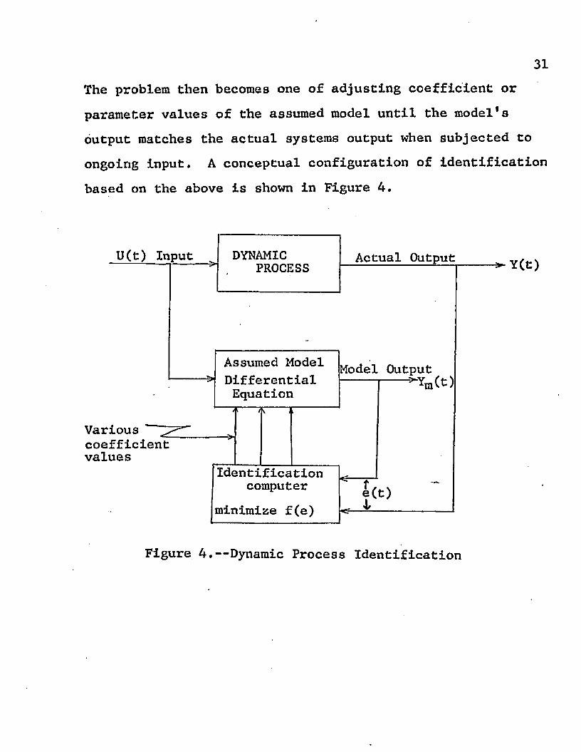
31The problem then becomes one of adjusting coefficient or parameter values of the assumed model until the model*s output matches the actual systems output when subjected to ongoing input. A conceptual configuration of identification based on the above is shown in Figure 4.

U(t) Input Actual Output

Model Output >Ym (t)

Various ^ coefficient values

e(t)

Assumed ModelDifferentialEquation

DYNAMICPROCESS

Identificationcomputer

minimize f(e)

Figure 4.— Dynamic Process Identification

32In order to develop a general purpose identification

scheme for biological phenomena, the modeling is limited to a differential equation form (a transfer function is a control system description of linear differential equation).

A dynamic system can be described, in general, by an equation of the f o r m : 62

(2.6) kSL • Pr^) ~ 0rao

where:A„ are the unknown coefficients describing

JL

the systemPr (t) are time dependent variables appearing in

the general dynamic equation. In the most general case these would include the input variable and its derivatives, the output and its derivative or combinations of these.

Therefore, equation (2.6) may be used to describe either a linear or nonlinear process.

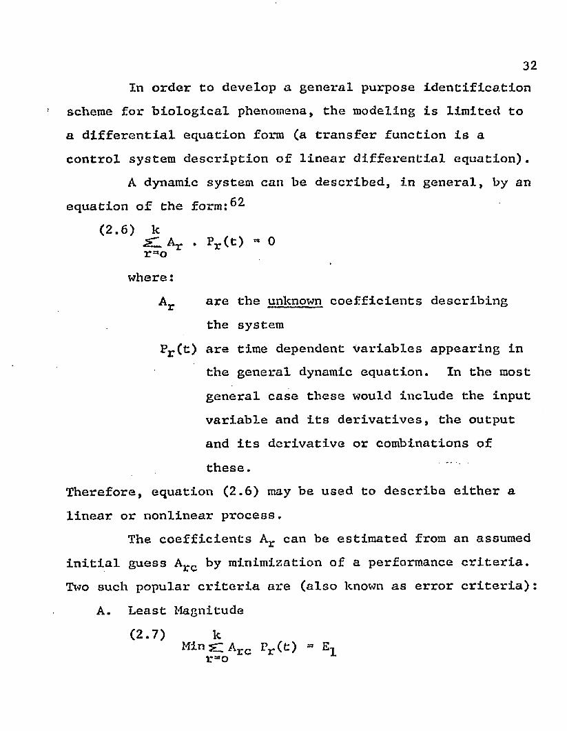
The coefficients Aj. can be estimated from an assumed initial guess Aj.c by minimization of a performance criteria. Two such popular criteria are (also known as error criteria):

A. Least Magnitude(2.7) k

Min 5EI Arc Pr (t) - E-, rao

33

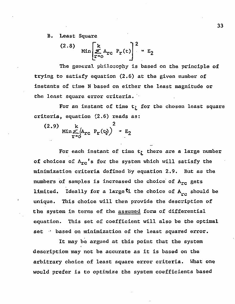
(2.8) P k *12MinLg:Arc Pr (t) - E2

r*oL _Min

The general philosophy is based on the principle oftrying to satisfy equation (2.6) at the given number of instants of time N based on either the least magnitude or the least square error criteria.

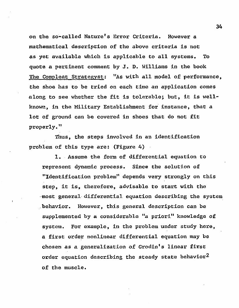
For an instant of time t^ for the chosen least square criteria, equation (2.6) reads as:

of choices of Arc's for the system which will satisfy the minimization criteria defined by equation 2.9. But as the numbers of samples is increased the choice of Arc gets limited. Ideally for a largeti the choice of A should be unique. This choice will then provide the description of the system in terms of the assumed form of differential equation. This set of coefficient will also be the optimal set ‘ based on minimization of the least squared error.

descriptiom may not be accurate as it is based on the arbitrary choice of least square error criteria. What one would prefer is to optimize the system coefficients based

For each instant of time t* there are a large numberu

It may be argued at this point that the system

34on the so-called Nature*s Error Criteria. However a mathematical description of the above criteria is not as yet available which is applicable to all systems. To quote a pertinent comment by J. D. Williams in the book The Compleat Strategyst: "As with all model of performance,the shoe has to be tried on each time an application comes along to see whether the fit is tolerable; but, it is well- known, in the Military Establishment for instance, that a lot of ground can be covered in shoes that do not fit properly.11

Thus, the steps involved in an identification problem of this type are: (Figure 4)

1. Assume the form of differential equation to represent dynamic process. Since the solution of "Identification problem" depends very strongly on this step, it is, therefore, advisable to start with the most general differential equation describing the system behavior. However, this general description can be supplemented by a considerable "a priori*1 knowledge of system. For example, in the problem under study here, a first order nonlinear differential equation may be chosen as a generalization of Grodin*s linear first order equation describing the steady state behavior^ of the muscle.

352. Assume an initial set of parameter values X:

*1

3* Based on this vector A, the assumed model differential equation is solved and the response Yra(t) for the ongoing input U(t) calculated.

4. The "identification computer" compares the model response Ym (t) with the observed output Y(t) and generates a new set of parameters in accordance with a chosen performance criteria.

The error function, then, may be defined as:(2.10) e (t, A) - Ym (t, A) - Y(t)

In absence of any knowledge of Nature*s Error Criteria, the performance criteria used in this study Is the least square error (equation 2.8). Thus, the problem of identification is reduced to a search for the minimum of the performance criteria or an optimization problem.

So far nothing has been said about the parameter values. In most problems of physical origin the parameters are constrained to be positive for a passive system, e.g., the parameters of a second order linear control system. Hence, the minimum of performance criteria E2 must be sought within

a well-defined region in parameter space. Another problem concerns the uniqueness of the minimum. Since most optimi­zation procedures operate on a local excursion principle, the solutions obtained can only be guaranteed to be local minima. For error functions having a unique minimum in the allowed region of parameter space, this poses no problem, but in most cases this information of unique minima is not readily available. Limited assurance of uniqueness of the minimum may be obtained by repeating the optimization, starting each time with a different set of parameters, and observing whether the convergence is always to the same point.

With the availability of a rather large number of optimization techniques to find the minimum of a given

C fLperformance criteria"* it is desirable to evolve the best technique to solve the particular problem posed in this dissertation. The term best in this context refers to limiting the number of functional evaluations in search for the final solution. With this aim, some of the important optimization methods are reviewed in Chapter III.

SummaryThe present techniques of characterizing left

ventricular behavior in systole and their shortcomings in defining the diastolic behavior has been discussed. The in­adequacies of Noble and Grodins models of diastolic behavior have also been pointed out. A systematic procedure utilizing

the system input-output variables for characterization has been described in this chapter.

CHAPTER III

REVIEW OF APPLICABLE OPTIMIZATION METHODS

IntroductionThis chapter briefly reviews the optimization methods

applicable to the differential equation parameter identifi­cation (DEPI) problem. This is done in order to provide background information toward development of an "Optimum Minimization Algorithm" (OMA) which combines the best features of the available techniques to solve the problem posed in this study. Best in this context refers to minimizing the number of functional evaluations required in obtaining the optimal solution of a given objective function. Appendix D summarizes the general properties of the optimization techniques and provides the necessary theoretical details. A particular search method known as "Reverse Golden Section Method" (RGSM) has been devised in the chapter as part of this study. The purpose of this technique is the computation of an optimal distance to be moved in the negative gradient direction, or a chosen direction, for minimization problems.

38

39

Objective Function DefinitionIn the case of the DEPI problem under consideration

the parameters, A, are real variables and the objective function F(A) is computed as:

(3.1) F(K) - (YT - Yc)* (YT - YC) where:

W " The observed data pointsYC “ Model response at the parameter vector H.

Optimization techniques discussed deal with minimi­zation of (3.1) with the parameters £ being constrained in the parameter space by the following:

(3.2) AL^rA^AH where:

AL Lower bound on the parameter valuesSH Upper bound on the parameter values

Search MethodsSpecific search methods considered in this dissex*tation

have been subdivided based on the number of unknown para­meters (i.e., dimensions in parameter space):

1. One-dimensional search methods2. Multi-dimensional search methods

One-dimensional Search MethodsThese methods are applicable for optimization of

functions of a single parameter (variable). Consideration

40of one-dimensional search techniques is important, since many of the efficient multidimensional search methods involve, at various stages of computation, a search for optimum along a particular direction. There are many one-dimensional search methods available, 6,57 The following have been selected on the basis of their application in solving the multidimensional type of DEPI problem presented here:

1. Quadratic Interpolation Method (QUAD)2. Pierre's Interpolation Scheme (PIS)

■ 3. Reverse Golden Section Method (RGSM)

Quadratic Interpolation Method (QUAD)This search method computes an optimal distance to be

moved in the negative gradient, or a chosen direction using Powell's interpolation formula. This formula is based on three function values defining a quadratic.^ A more detailed description of this technique and the adaptations necessary for its use in the available computer are given In Appendix D. This method can easily be modified for multidimensional problems and has been coded as such in Appendix A.

Quadratic Interpolation Method has also been used in conjunction with various multidimensional methods in Chapter V. These techniques require search along a given direction for function minimization of each iteration step and are discussed in detail later in this chapter. When used

with discrete steepest descent, QUAD requires the least number of functional evaluations for the greatest reduction in function value at a given iteration step (Chapter V).When the function value is small (indicating the closeness of an optimum point in case of DEPX problems), the number of functional evaluations required with QUAD are greater than with RGSM. Therefore, as discussed in Chapter V, QUAD is used when both the magnitudes of the gradient vector and function value are large (signifying points away from minima). The search using RGSM is carried out when the gradient vector has been reduced substantially. Both these methods used in the above described manner proved superior to PIS.

Pierre's Interpolation Scheme (PIS)Tliis scheme computes an optimum multiplier based on

Davidon's formula. The above technique has been modified from Pierre^ In this dissertation for use in development of OMA. Appendix D gives programming details of the method.This method has also been used as a one-dimensional search with multidimensional methods which require search along a given direction for minimization at an iteration step. As will be seen in Chapter V, this method is inferior compared to RGSM and QUAD for DEPI problems when used ir. conjunction with the discrete steepest descent.

42Reverse Golden Section Method (RGSM)

It has been shown by Wilde that the number offunctional evaluations for minimization is the lowest, for agiven level of tolerance in parameter value, with a search

57method using golden section ratios. The search utilizing such ratios is known as ’'Golden Section Search" and is briefly described in Appendix D. In the application of the method, it must be known that the optimum lies between two given values known as width of uncertainty of the parameter A. In most cases of practical application, this width of uncertainty, in a given direction, is not known "a priori."In order to exploit the proven efficiency of Golden Section Search, in a one-dimensional problem, RGSM was developed in this study. This attempt has been made here in order to find a most efficient method of handling the DEPI problem.

The procedure developed computes on "optimum" distance to be moved based on golden section ratios. In the case of the DEPI problem, the initial interval^d^jin which search is to be conducted is not known a priori. (That is to say the optimal distance to be moved in the negative gradient direction at each iteration step for function minimization is not known.) The search plan is based on establishing a unimodal function description in a given direction and thereby determining d^, the interval of

43uncertainty. Once the interval to be searched, d- , has been bounded, "Seardh by Golden Section" may be carried out.

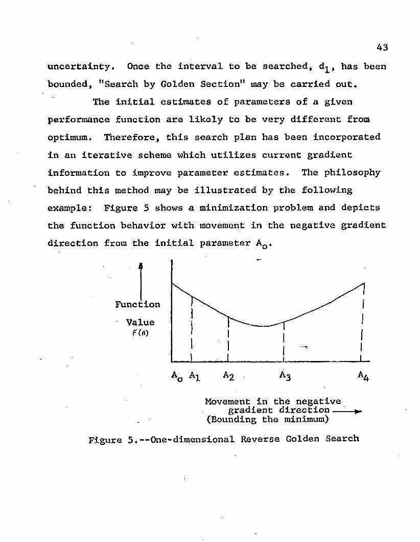
The initial estimates of parameters of a given performance function are likely to be very different from optimum. Therefore, this search plan has been incorporated in an iterative scheme which utilizes current gradient information to improve parameter estimates. The philosophy behind this method may be illustrated by the following example: Figure 5 shows a minimization problem and depictsthe function behavior with movement in the negative gradient direction from the initial parameter A0.

i\

FunctionValue

F(fi)

Ao A1 A2 a3 A4

Movement in the negativegradient direction — —

(Bounding the minimum)Figure 5.— One-dimensional Reverse Golden Search

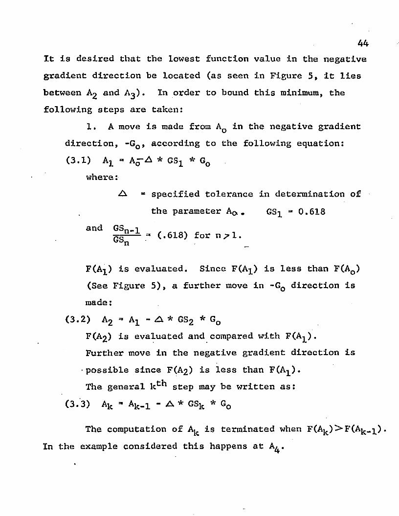
44It is desired that the lowest function value in the negative gradient direction be located (as seen in Figure 5, it lies between A2 and A3). In order to bound this minimum, the following steps are taken:

1, A move is made from AQ in the negative gradient direction, -G0, according to the following equation:(3.1) Ax « Aq A * GSX * Gq

where:A « specified tolerance in determination of

the parameter Aq, . GSX =* 0.618and GSn_x

Gsn (.618) for n^l.

F(AX) is evaluated. Since F(AX) is less than F(AQ)(See Figure 5), a further move in -G0 direction is made:

(3.2) A2 a Ax “ A * GS2 * GqF(A2) is evaluated and compared with F(AX).Further move in the negative gradient direction is •possible since F(A2) is less than F(AX).The general k*"*1 step may be written as:

(3.3) Ak - Ak_x - A * GSk * Gq

The computation of Ak is terminated when F(Ak) > F(Ak„x) In the example considered this happens at A^.

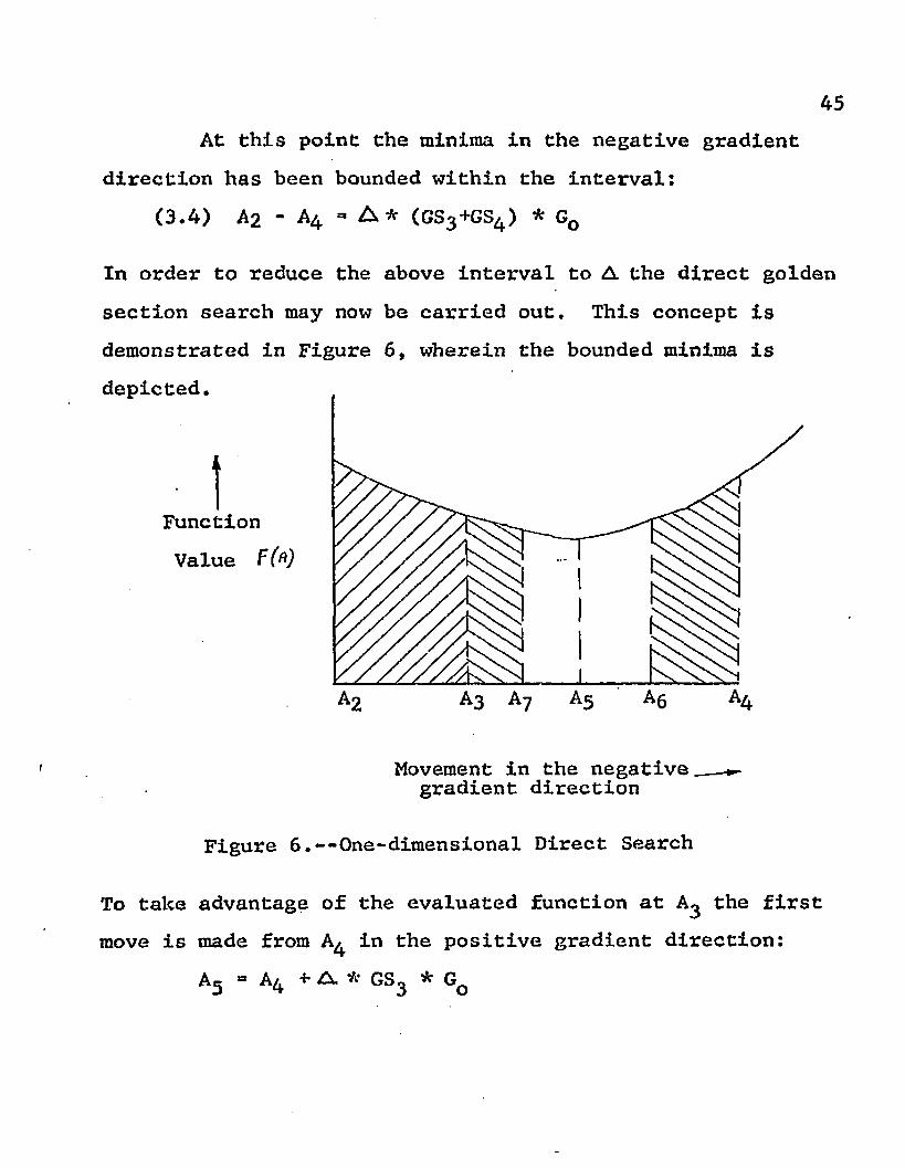
45At this point the minima in the negative gradient

direction has been bounded within the interval:(3.4) A2 - A4 - A * (GS3+GS4) * G0

In order to reduce the above interval to A the direct golden section search may now be carried out. This concept is demonstrated in Figure 6, wherein the bounded minima is depicted.

To take advantage of the evaluated function at A^ the first move is made from A4 in the positive gradient direction:

A5 » A4 + A * GS3 * GQ

Function Value F(A)

A2 A3 Ay A5 Aq A4

Movement in the negative gradient direction

Figure 6 .--One-dimensional Direct Search

46Since F(A5)<;1 F(Ag) the region between A£ and A3 cannot contain the minima without violating the unimodality condition and is, therefore, eliminated from consideration. The interval in which the minima lies has thus been reduced to A * GS4 * G0 . The next move is again made from A^, since A£ was modified at the last step.

(3.5) A6 - A4 + GS2 * G0Since F(Ag)7 F(A5) the minima may not lie in the region between A^ and Ag and this area may be discarded. With this step the interval in which the minima lies has been reducedt O A * G S 3 * Gq.

The next move is made from A3, since A4 was eliminated in the last move:

(3.6) Ay " A3 + A * GS^ * GoSince F(Ay)7F(A5) the region between A3 and Ay may not contain the minima.

Thus, the minima is located between Ay and Ag within an interval of ^ * GS2 * GQ * A * GQ. Since G0 is normal­ized to unity the accuracy in parameters is A .

The number of functional evaluations required in locating the minimum at A5 are:

Number in bounding the minimum + Number in Golden Search 0 4 + 3 “ 7

47In general the total number of required iterations

is given by 2k-1 where k is the number of functional evaluations necessary to bound the minimum.

This method can be easily adapted for multi­dimensional problems and has been coded as such in the next chapter as a subroutine (RGSM).

For parameter values far away from the optimum point, the gradient vector may not point in the exact direction of optima. In such cases, the parameter values need not be computed with die same rigorous accuracy. This enables the search to be accelerated. Once near a stationary point, signified by small gradient magnitudes, the search may be conducted with the required accuracy. This provision has been included in the "Reverse Golden Section Method" (RGSM) programmed in Chapter IV.

In order to determine the true nature of the stationary point thus obtained, other search techniques which utilize second order derivative information must be used. Chapter V describes the results obtained using RGSM for determination of the optimal multiplier in discrete steepest descent search. Near the optimum point (characterized by small function values) this method is superior to both QUAD and PIS.

The three search methods programmed and coded in this dissertation have also been used with the Fletcher-Powell

48Method, Fletcher-Reeve Method, and continued PARTAN (see the following pages). These methods require one-dimensional search for minimum at various iteration steps. Chapter V describes the results obtained with these methods.

Multidimensional Search MethodsThese methods are applicable for optimization of

functions of several parameters (variables). Appendix D discusses the difficulties associated with optimization of multidimensional problems. Of the many available search techniques, the following have been selected for application to the DEPI problem posed in this dissertation.

1. Random Search2. Discrete Steepest Descent3. Least Square Minimization Method4. Conjugate direction methods5. Acceleration Step Search6 . Pattern Search

Random SearchAs the name implies the function F(X) is evaluated

at points which are randomly chosen within the feasible parameter space-. The parameter values, at which the lowest function value is obtained in a specified number of functional evaluations, are designated as the optimum. The principal

49attribute of random search is that it has no innate bias, something which is always found in nonrandom methods. Two variations of random search have been utilized in this dissertation. They are:

1. Random search to choose a starting point. In this variation a random search is carried out in the entire permissible parameter space to locate a starting point. This type of search in the absence of a reasonable estimate of parameter values leads to a more efficient minimization than in methods with arbitrarily chosen starting points. Once the starting points are located the more powerful sequential search methods can be used. Since the parameters of the proposed ventricular model are not known "a priori" this search provides starting parameter values.

2. Random search to determine the nature of stationary point. Once near a stationary point, the sequential search methods, which are based on current gradient information, converge to this particular solution. In cases where the stationary point represents a point of inflection the solution thus obtained is not optimum. To determine the true nature of the stationary point, a random search is carried out around the current optimum solution. If the search around the current optimum

point reveals that a lower function value is available then the search is continued using sequential methods from this point. In case no lower function value is obtained in a specified number of random searches around the current minimum point, then one is reasonably certain of the location of a minimum point. In the particular case of DEPI problems the minimum of F(A) is given by zero; this variation of random searching is employed to locate a more favorable parameter vector around the current stationary point (characterized by very small gradient magnitude and a positive function value). Thus, convergence to a false minima may be avoided.

Discrete Steepest DescentThis method Is based on the truncation of the Taylor

series expansion of the objective function F(A) after the first two terms. This method utilizes only the gradient information and, therefore, may not yield a good approxi­mation of the function behavior for problems in which the second order derivatives are not negligible. In the particular case of DEPI problems it is known that the minimum function value is zero (where the model response exactly matches the observed data). Therefore, a linear interpolation to zero may be utilized to compute the para­meter change vector AA. The new parameter vector is taken as

51

Anew . “ A + A A if F(5_ )<= F(A) (For steepestU c W

descents A is in the negative gradient direction.)In a variation of the discrete steepest descent known as "optimum steepest descent" a one-dimensional search is incorporated to obtain an optimal<AA at each iteration step (see Appendix D for details).

It has been shown that this designation is misleading and quite often improvements in convergence can be made by Incorporating features from the geometry of the objective function.$6 This approach of computing the optimal distance to be moved using a one-dimensional search has been used in this study without naming this as the "Optimum Steepest Descent." The results (Chapter V) show the inferiority of the discrete steepest descent applied to the DEPI problem in comparison with LSMM.

Least Square Minimization Method (LSMM)

As described in Appendix D, the chief drawback of thec cNewton's Search is the computation of second partial

derivatives at each iteration step in addition to the gradient. In this study the objective function has been cast in the form of sum-squared error between the observed response YT and the predicted model response YC and approximations to the second order derivatives are generated

52as part of the effort involved in computing function value and the gradient (see Appendix D for details). Since a Taylor series expansion involving second order derivatives in addition to the gradient information provides a better approximation of function behavior than the one using only the gradients near the optimum point, this availability of second order derivative approximation has been exploited. Least Square Minimization Method (LSMM) has, therefore, been coded and programmed for use in this study. Appendix D gives the theoretical details of the method and the programming details are given in Chapter IV. To be useful, LSMM requires a program for matrix inversion, and this may be a limiting factor in use of LSMM for DEPI problems having a large number of unknown parameters. Chapter V describes the results obtained using LSMM and its excellent convergence properties as applied to the DEPI problems.

Conjugate Direction MethodsThe conjugate direction methods herein described

provide, in general, a faster rate of convergence compared with basic gradient methods. Conjugate directions are defined with respect to a quadratic function.

If a quadratic function to be minimized is given by:(3.7) f(x) =* x*£a]x + F'x + c

53then the directions p and q are defined to be conjugate directions if:(3.8) p*ZA]q - 0

For a minimum to be definedCA3must be positive definite.

It has been proved by Powell^ that the minima of a well-behaved n dimensional quadratic function can be located by search along each of the n mutually conjugate directions only once. Thus, the problem of solving an n-dimensional case is resolved into n one-dimensional problems.

In the general case of optimization of non-quadratic objective function, the method is applied in iterative steps. After n one-dimensional searches along the mutually conjugate directions from the given estimate of parameters X, a better

iestimated A is reached. The process is then repeated withX1 as the initial parameter vector until a specifiedconvergence or tolerance criteria is met. There are anumber of ways by which mutually conjugate directions can

79be generated. Powell describes a simple method in which, starting with movement in given parameter direction, the other conjugate directions are generated as part of computational process. Two modifications of the basic Powell method which use the current gradient informations

54to generate conjugate direction are currently quite popular in minimization problems.

1. Fletcher Reeve Method2. Fletcher Powell Method

Fletcher Reeve Method80In this variation the conjugate directions rH are

obtained in sequence by the following computations:(3.9) R° «* - G°

(3.10) Rk+1 “ - Gk+1 + ■ «a^ k'KL? ' k-0,1,2....

where:G° is the gradient of F(A) at the initial point A°. G c+^ is the gradient of F(A) at the point /?c+l The point A^*^ is determined by the following

relationship:(3.11) F0?c+1) - rain F(A^ + <*Rk)

(For details of theoretical justification, seeFletcher and Reeve^) .

In using this method it is recommended that at leastM one-dimensional searches be effected regardless of other

80stopping criteria. The search may be terminated either when a specified number (N) of one-dimensional searches have

_ . Tf 1 _ i .been completed or when both the value of (G .(*) and the

55value - A^)1 (A^+^ - T iJ are diminished belowpreassigned levels. The equations (3.9) and (3.10) are coded in a subroutine UPDATE (Appendix A) for use toward development of OMA in Chapter V.

Fletcher Powell Method^This method is to date the best single method

available for the following type of problem:(a) F(A) is given analytically and both first and

second order partial derivatives exist.(b) Evaluation of F(i£) and VF(?i) require a relatively

large amount of time as compared to that required for matrix manipulations associated with this method.

This method generates the inverse of Hession Matrix/djafter M one-dimensional searches without the explicitcalculation of second partial derivatives. This may mean aconsiderable savings in computational time. By making useof second order partial derivative approximations at eachiteration step a better expansion of objective function isobtained as well.

The general procedure of the Fletcher-Powell method78for minimization is as follows:

1. A s s u m e “ I and the initial point to be A°2. At the iteration step calculate the gradient

vector &

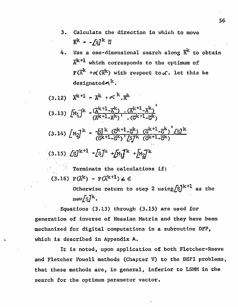
563. Calculate the direction in which to move

& - -^s/k 5- v4. Use a one-dimensional search along to obtain

—k+1A which corresponds to the optimum of F(/v with respect to<sC- let this bedesignated*^.

(3.12) 3k+1 » 3^ +«<k .ldc

(3 13) /Jl,1k - . (5k+:l-ak)'(3.13) £My (5k+1.sk), .(ck.-l.gk)

(3.14) fth7k - k '/S7k.L 2J (£k +1 -gK) 1 /5jTk (Gk+1 -G )

(3.15) z?7k+1 =/iJk +^IlJk + ^ k

Terminate the calculations if:(3.16) F(Ak) - F(Ak+1) £ £

Otherwise return to step 2 using^sjk+^ as the n ew/y k .

Equations (3.13) through (3.15) are used for generation of inverse of Hessian Matrix and they have been mechanized for digital computations in a subroutine DFP, which is described in Appendix A.

It is noted, upon application of both Fletcher-Reeve and Fletcher Powell methods (Chapter V) to the DEPI problems, that these methods are, in general, inferior to LSMM in the search for the optimum parameter vector.

57Acceleration Step Search

Acceleration step search methods combine the featuresof gradient techniques with the geometric aspects of theobjective function. These methods were first described by

81Forsythe and Motzkin for the specific case of functions with two unknown parameters. Shah, et al.**2 extended this approach to problems with n-variables and devised the method of parallel tangents (PARTAN). A popular variation of this approach is known as continued PARTAN.

This method consists of alternate searches along the following directions:

1. Search along the negative gradient direction assuming minimization to generatek » 0,1,3,5,7,9,11 — - 2k+1.

2. Search along the direction defined by A2k-A2lc“3 k “ 2,4,6,8 —

This above direction is known as acceleration step.When k - 1 the search is conducted along the direction A2-A°.

82It has been shown by Shah, et al. that the exact optimal point is located, after 2n-l one-dimensional searches for an n dimensional quadratic function PCS'). The programming details of this method are described in Chapter IV. In the particular case of the DEPI problem, this method, while

58showing superiority over the discrete steepest descent, is less efficient than LSMM for function minimization (Chapter V).

Pattern SearchThe pattern search technique devised by Hooke and

8 3Jeeves owes its existence to the simple-minded ability of a digital computer to carry out vast numbers of arithmetic operations fairly rapidly. Pattern search is carried out in two separate operations:

1. Exploration moves2. Pattern moves.The general approach of pattern search is to make a

local "Exploratory Move" search in order to seek out a promising direction and then to actually make a larger "pattern" move in this direction. Attempts are made to establish the "pattern" of successful search points in the immediate past from which possible future points are predicted.

The programming details of pattern search as used in this study are given in Chapter IV. Upon application of pattern search to the DEPI problems (Chapter V), it Is observed that this method yields poorer convergence (slower reduction in function values) than LSMM.

SummarySeveral optimization techniques have been briefly

reviewed in this chapter and their relative merits discussed.

In order to ascertain the optimal distance to be moved in a given direction for optimization, a method named "Reverse Golden Section Method" (RGSM) has been developed. All the optimization methods considered in this chapter have been programmed (Chapter IV) and used toward development of the OMA in Chapter V.

CHAPTER IV

PROGRAMMING AND COMPUTATIONAL ASPECTS OF THE APPLICABLE MINIMIZATION METHODS

IntroductionThis chapter provides the programming details of the

various minimization schemes discussed in Chapter III. All programs described in this chapter have been programmed and coded for use toward development of the "Optimum Minimization Algorithm" OMA in Chapter V. The programs developed in this chapter deal with the constrained optimization (parameter range restricted) of the DEPI problem discussed in Chapter II.

General CommentsThe optimization methods described in Chapter III

have been programmed for use on the IBM 370/165 .computer.This has been done with a view to facilitate development of the proposed OMA for solution of the DEPI problem. Due to the requirement of physical interpretation of the proposed ventricular model, the parameters must be constrained to be positive and physically realizable (this has been discussed in Chapter II). Since none of the minimization schemes discussed in Chapter III are available as "CANNED PROGRAMS"

60

61for solution of a constrained minimization problem it is necessary to develop these schemes for computer implementation. It is also felt that due to the constraints posed on the parameter values, the efficiencies ascribed to various search methods may not be applicable. Further, there has not been a study of the minimization methods relative to the DEPI problem. Therefore, the constrained parameter search methods (Chapter III) have been programmed here for comparison of their efficiencies and possible use with OMA.The results of computer runs on known differential equation forms using the search methods programmed in this chapter are described in Chapter V.

All the methods described in this chapter deal with the DEPI problem. However, these methods may readily be modified for other minimization problems by writing sub­routines for:

1. Evaluation of objective function (SQRERF.) and2. Approximation to the gradient of the objective

function in parameter space (APGC).The actual coding of the subroutines used In this

dissertation Is listed in Appendix A.

Implementation of Constraint Conditions in the Search Procedure

There are several ways in which these constraints may be accommodated. Two possible variations are:

621. Augmentation of performance criteria (objective

function).2. Parameter check at each iteration step.The philosophy behind the augmentation approach is

to substantially increase (in case of minimization) the value of performance criteria in case of constraint violations.

This is done by adding a penalty function to the unconstrained performance criteria. The penalty affects the performance only in case of constraint violations. Pierre describes several ways of incorporating the penalty function. However, in the particular problem posed in this dissertation it is simpler to check the parameter values of each iteration step.

This method is a slight variation of McGhee* approach of gradient projection. In this variation the components of parameter vector A are checked for range violations. In case a particular range constraint is violated, the corresponding component of parameter vector is reset to its previous value. If a move violates range constraints in every component direction, no further compu­tations are carried out using that particular move. A separate subroutine GRADM for move modification, used in this dissertation, has been described in Appendix A.

Programming AspectsThe methods programmed in relation to development

of an optimum minimization algorithm, OMA., are:1. Least Square Search Method (LSMM)2. Pattern Search Method (PATERN)3. Random Search Method (RANSER)4. Reverse Golden Search Method (RGSM)5. Search using "continued PARTAN"6 . Search using Fletcher-Powell Method7. Search using Fletcher-Reeve MethodIt is implicitly assumed in the following that

explicit methods for calculation of function value and gradient are available.

The search techniques Fletcher-Powell method and Fletcher-Reeve method are based on equations described under conjugate direction methods (see Chapter III). The actual coding details are given in Appendix-A. 3>nd the one­dimensional searches at various iteration steps have been carried out using the three interpolation subroutines; namely, RGSM, QUAD, PIS. Chapter V discusses the results obtained using these methods as applied to the DEPI problem.

Least Square Search Method (LSMM)This method is based on the following equation which

is detailed in Appendix D, equation D.26.

64(4.1) Z - ®M*M N*M

where:Z =* parameter change vectorE » YC - YT

a Model ErrorDeviation matrix defined in Appendix D.

At each iteration step 2 is evaluated and the new parameter vector K is computed using:

(4.2) £ - &>+ ZFurther iteration is continued with "K only if:

F(A)^F(A°)A step-by-step description of the programming sequence

is detailed with reference to Figure 7.1. Explicit form for computation of function value

F(A) is available. The initial parameters vector AO, function value F(So), the gradient (5 (AO) " L.<t>3 E and the matrix are available. Upper and lower range constraints on parameter values AH and AL and the number of parameter’s N are also given. M is an indicator of success/failure of the method at a given iteration step.

2. Both G andfi/^jare normalized using Marquardt's formula (see Chapter VII). The equation (4.1) is solved using the IBM library subroutines SIMQ and ARRAY (Appendix A).

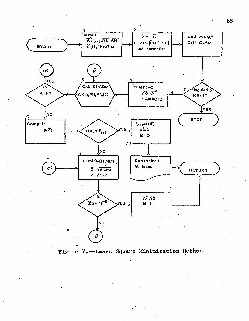
65

C a ll ARRAY C all S IM Q

Z = - G

T E M P = |P H I’ PH[] and normalizeS T A R T

YES/ Call GR ADM

{ a ,z ,n ,a h ,a l ,k )

TEMP3=^Za'o = a 0 ■ A=AO +Z

K =N ?

YESNO

STO PCompute

F(A)

NO

ConstrainedMinimum

TEM P3=TEM P3

RETURN

NO

Figure 7.--Least Square Minimization Method

i

663. In case the determinant of Qt> ' i s zero,

implying singularity, further computation is not carried out. This condition is indicated by KS’l.

4. If KS Is not equal to one, the computation in SIMQ proceeds and the computed parameter change vector2 and initial parameter vector S° are saved in temporary locations TEMPS’ and AO respectively.

The new parameter vector is generated according to the following:(4.3) A - AO + Z

where ~R is the new vector and 7SJ is the old parameter vector.

5. A check is made of the values of A. If the new vector violates all the range constraints, a counter K is set equal to number of parameters N in the GRADM subroutine and control is transferred to block 7.

6. The function value of A, F(A), is. computed.If F(X) is less than F(AO), then both F(S0) and SU are modified according to:

F(£0) - F(A)AO - A

A success message is written and control is transferred to calling program with Ma0.

67

7. In case F(A)>F(AO) or K°N, the computed change vector Z is halved .Z ** Z/2 and a new vector A is generated:(4.4) A * IS + 1./2If (Z* Z)J# is less than 10“^ (nominally) it is assumed that no significant improvement is possible and control is transferred to calling program with M^l, which indicates failure of the method. For 0Z.% 2)^ greater than 10"^ control is transferred to block 5.

Pattern Search MethodThis method has been programmed as two interacting

subroutines, PATERN and EXPLOR. As the name suggests, the subroutine PATERN is responsible for pattern moves and also controls the execution of exploratory steps. Actual exploration is implemented by the subroutine EXPLOR. The details of both of these programs are given below.

Subroutine PATERN.--The computation events may be described with reference to Figure 8.

1. Explicit forms for computation of F(A)(Appendix A) and exploration moves are available.Initial estimate of parameter vector A°, initial function value F t, EPS (parameter indicating magnitude of change in parameters), upper and lower constraints on

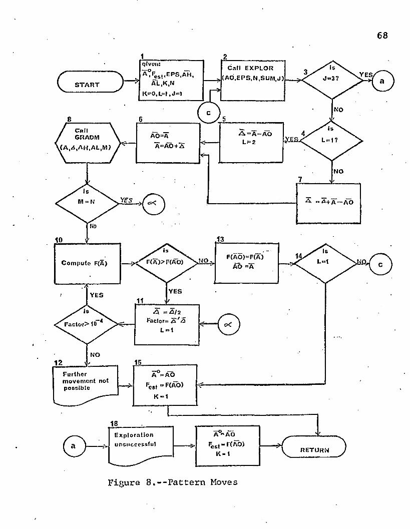
68

given:

A, i,sj,EPS,AH, AL,K,N

K=70,L=1, J=1

Call EXPLOR (AO.EPS.N.SUM.J) y e s

S T A R T

/ Call ' GRADM(A .A .A H .A L .M )

NO

M = N

NOF(A)>F(AO)Compute F(A)

YESYES

Factor> 10

NO

Further movement not possible

A " AO

rcst-r °)K-1Explorationunsuccessful

RETURN

Figure 8.--Pattern Moves

69the parameter values AH and 7lL and N, the number of unknown parameters are given. L and J are two constants used in the program and are initially set equal to 1 . K is an indicator of success/failure of the method and is initially set to zero,

2. An exploration move is made to improve the parameter vector A by calling EXPLOR. If exploration is unsuccessful, J is set equal to 3. Otherwise, J is set equal to 2.

3. If 3=3 then a diagnostic message indicating the failure of the exploration move is written and control is transferred to the calling program with 10*1.

4. A check is made as to whether it is the first time that the exploration routine is called. L not equal to one signifies that an old pattern exists which may be modified. In this case, control is transferred to block 7. ;

5. The vector A, initial pattern vector, for moves in the same direction which proved successful in the exploration stage is computed and is set to 2, signifying that exploration has been made at least once in the current search.

6 . The initial parameter vectors 7d3 is set equal to *£, the successful parameter vector resulting from

70the exploration. A new parameter vector is generated according to the following equation:(4.5) A - AO + 5.and control is transferred to block 8.

7. The existing pattern vector is modified according to the following:(4.6) A * S + A - AO

where: AO is the "old" parameter vector from whichexploration moves were made and "K is the "current" parameter vector from successful exploration.Control is transferred to block 6.

9. A check is made on the number of constraint violations, M, if M^N (implies no move possible without violation) control is transferred to block 11.

10. F(X) is computed and the current parameter point A and a comparison is made with the old value of function at F(AO). If F(7C) F(A0) then control istransferred to block 11 for making a smaller pattern move. Otherwise control is transferred to block 13.

11. A smaller pattern move is made but the "pattern" is preserved,

S - S/2

Factor * (A1 A)If Factor indicating the magnitude of present pattern

move is less than 10"^ (arbitrary), then it may not be

71worthwhile to further pursue pattern search and, therefore, control is transferred to block 12. Otherwise, control is transferred to block 7.

12. A diagnostic message is given and the values of the function and the last "successful" parameters are returned.

10*1 and control is returned to the calling program.13. The current successful parameter vector is

saved along with its function value and control is transferred to block 14.

14. A decision is made as to whether to continue to use the pattern available so far or to start a new pattern. Lal means a new pattern is to be built and control is transferred to block 15. If L equals 2, exploration is continued by transferring controls to block 2.

15. The "last" successful values of the parameter vector AO and function value F(A0) are returned to the calling program:

S° » SOFest " F(ro>

Exploration.""The steps involved in exploration with reference to Figure 9 are:

1. Explicit form of computation of F(X) is programmed. The initial parameter vector function value F(A0),

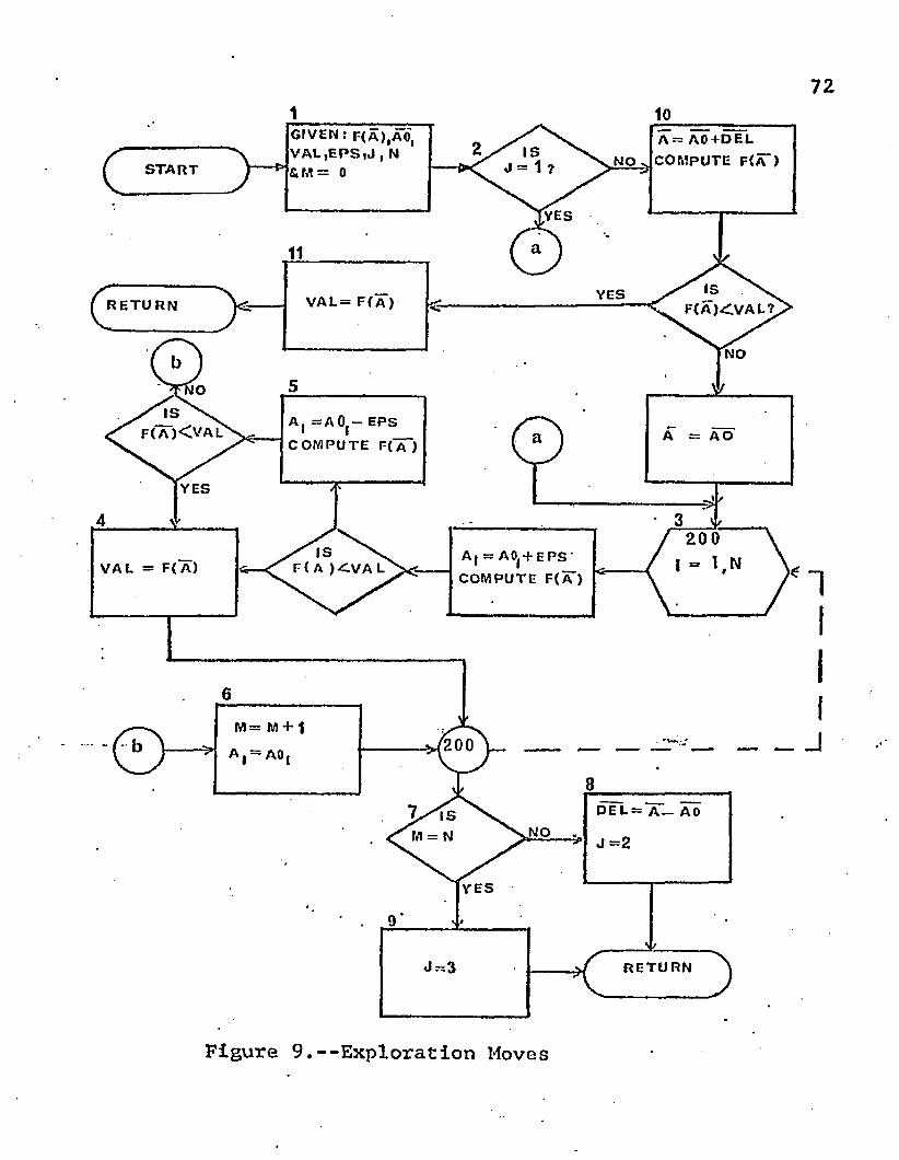
72

GIVEN r r(A),AO, V A L .E P S iJ , N &M= 0

A = AO + D E L COMPUTE F ( /T )IS NO

YES

YESV A L = F f A )R E T U R N

NO

A, =A0j- EPS C O M P U T E F ( X )

A = AO

YES

200A , = AOj+ E P S ' CO M PUTE F(A")

M = M + 1200

D E L = A — AO[s' ISM = N NO J=2

R E T U R N

Figure 9.— Exploration Moves

1

73EPS, J a control constant, and N the number of unknown parameters (dimensions of A vector) are given.

A counter M is set to zero, and£ - £S

J is initially set to one by the calling program. The program itself modified J in course of computation.When an exploration vector is available, J is set equal to 2 and when no exploration move is possible, J is set to 3.

2. If J is not equal to one, control is transferred to block 10.

3. Execution is carried out N times in this block. Starting with the iteration counter i**l. A displacement is made from £5 in the A, direction in parameter space,(4.7) At = A0± + EPS

and F(£) is evaluated. If F(£) is greater than F(£0), control Is transferred to block 5.

4. F(£o) Is modified to the lower function value F(A) and control is transferred to block 3 after updating the iteration counter i by 1,

5. A displacement in negative A^ direction is made:(4.8) Ai = A0i - EPSand the function value F(A) is computed if F(£) is less than VAL control is transferred to block 4.

746. Since there has been no "improvement" in either

direction in the counter M is incremented by 1 andis reset at AO^. The iteration counter i is

incremented by 1 and control is transferred to block 3.7. Once all the iterations have been carried out

if M*N then no move is possible from current point AO.In this case control is transferred to 9.

8. The "exploration vector" DEL is computed and Jis set to 2. This DEL is used the next time an exploration move is required. This is done in order to take advantage of the past successful exploration. Control is then returned to calling program,

9. J is set to 3, signifying that exploration is unsuccessful and control is returned to calling program.

10. The new vector A is computed from the past winner SO and the last successful exploration vector DEL. The function value F(A) is computed. If F(A) is less than F(A0) then F(AO) is set as new F(A) and control is returned to calling program.

If F(A)>F(A0) control is transferred to block 3. to calculate a new DEL vector and function value if possible.

75Random Search Method

The programming aspects of the method can be visualized with the aid of Figure 10. A step-by-step description of Figure 10 is given below:

1. Explicit forms for computation of function value F(A) and a random number are available. The upper and lower ranges on parameter values, number of random trials NT, number of unknown parameters N, a constant IXfor random number generation are given. A counter KR is set to 1 if a starting guess has been provided.

2. If KR is not equal to 1, a starting vector S' isgenerated by calling the random numbers routine RANPAR (Appendix A).

3. The parameter vector A is saved in location 3C and the computed function value F(A) is saved as SUMO.

4. A search is made by randomly generating A and“"computing F(A) and if F(A) is less than SUKO, thepresent function value and parameter vector are saved.

If the present function value is greater than SUMO, another random vector is generated in the first step above.

This is done for NT times.5. The final vector £=X gives the lowest function

value F(£) in NT attempts. Therefore, X and function value SUM=*SUM0 are returned to the main program.

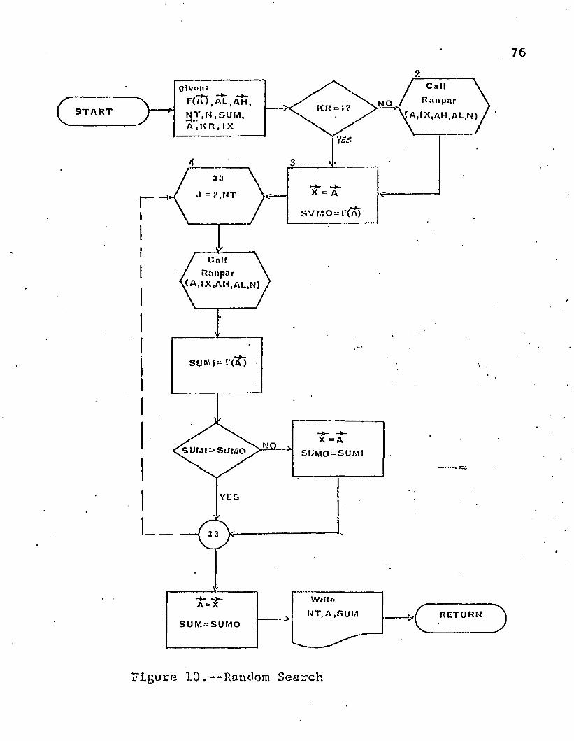
76

cS T A R T

C all

N O ^ KanpurCA.IX.AH.AL.N)

givenF(7t), A L .A H , N T , N t SUM, a '.KR, IX

J = Z ,N T

V M O = 1 :(A)

Riinpar ( A , tX ,A H (AL,N)

SUMi^F(A)

UlYiO UMO=SUMJ

“>— y- WriteA-X--------- NT, A ,SU M

S U M = S U M O

1

R ETUR N

Figure 10.-**Random Search

77Reverse Golden Section Method (RGSM)

The reverse golden search computes an optimal distance to be moved in the negative gradient direction. The sequence of computation events are described below with .reference to Fig. 11

1. Explicit forms for computation of F(A) is programmed. The initial parameter vector X°, the function value F(A°), Fest, the gradient vector <5 at X°, confidence interval C (nominally 10 J) specifying accuracy inparameters and golden section ratios F(I), I *■ 1,2- Kare given. The upper and lower range constraints on parameter values AH and XL are lcnown. The success/failure indicator M is initially set to zero.

2. In cases where the initial estimate of parameter vector X° differs considerably from the optimum vector the gradient G will be rather large. In order to speed up the minimization process, the confidence interval is modified with respect to the gradient magnitude.

R » (G1 G)^ is evaluated and the gradient vector is normalized.

If R ^ l control Is transferred to block 3 so that a larger confidence interval may be chosen.

Otherwise, ,Ais set to C and control transferred to block 4.

3. /%= C*R. This ensures that a crude minima would be located, since the confidence interval within which

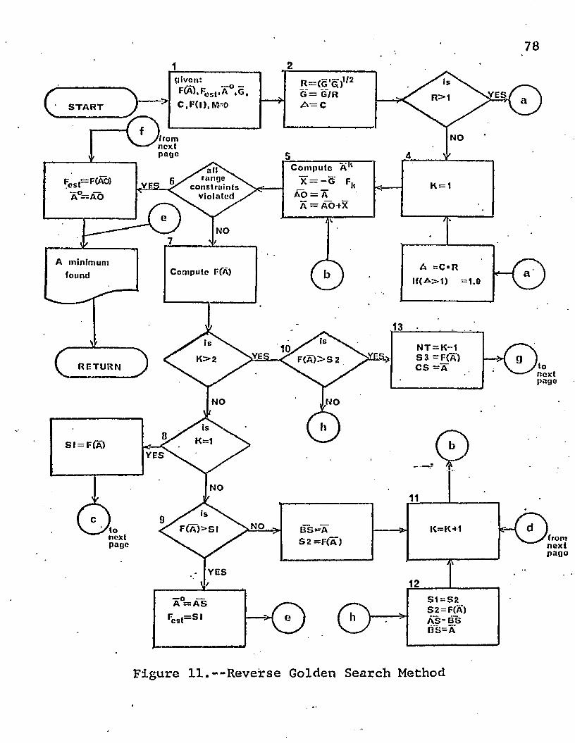
^ESR>1S T A R T

NO'fromnextpage

Compute AyatlXrange

constraintsviolated

ZZS.AO

AO+X

NO

A r=C«R l f (A > 1 ) «1.0

Compute F(A)

F (A )> S 2K > 2R ETU R N

nextpage

NO NO

YES

NO

NO K=K+1nextpage

fromnextpago

YES

■ OA = A S

Figure 11.--Reverse Golden Search Method

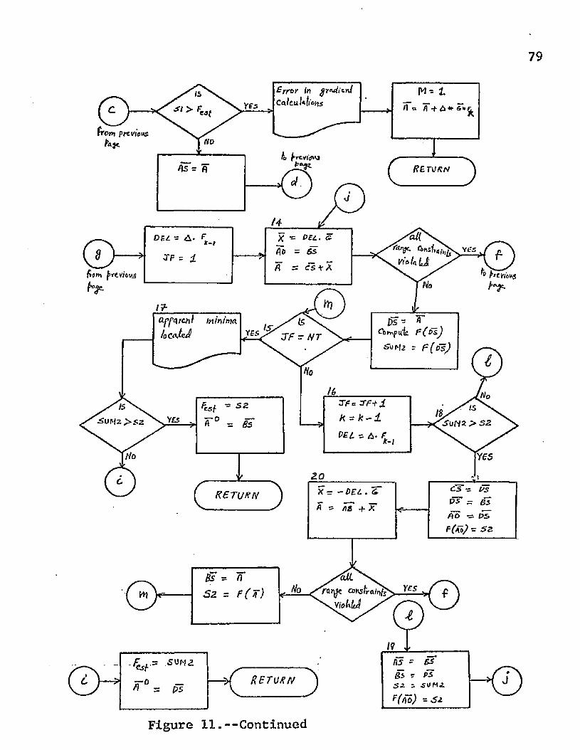
79

from previousI'AJt.As = a

Brror in gru^ierj n - 1

>.V f3 CalcuUfions rt = /)+£*■

It, /■rtyicfWJ

Is

■ ©

0from previous14

^ RE TURN

D K 3 A * F* - fX - t>££. G-

TF = i — — > (\t> - 6S

A r: CS t A

apf<*rt)if m in im a

loCaleJ

U

])S * «p ( o s j

S itH i = F ( o s )

F«* - 52w° = fis

Spa ZTF’t X k-k-1KL - *■■ 5-,

RETURN 320

Suns,

X - - O E L . 6

. 1 » ---------__■C 5 - P 5

•* -- OS' = BS=■ (\& + X •f-----------

/)£> •= D 5

F AV -

&Bs - n

tlo sS Z = f 'farge a*sUi >j£L+f f ) jviokU s''s \ yCl)

19£.,.= smz

R E T U R N

ns -. .ts

Si p PSSi - SUMZ

- Si- * ©

Figure 11.--Continued

80it lies is larger than the specified interval. If is greater than 1, it is reset equal to one so that the computations may be possible even when the gradient magnitude is large.

4. A counter K is initialized to 1.5. The new parameter vector at the k*-*1 reverse

golden move is generated by moving in the negative gradient direction.(4.9) ^ » Ak_1 - A* G*Fk

6. A check is made on the number of constraint violations. If all range constraints are not violated, implying that the current vector lies in the feasible region, control is transferred to block 7 for further computations.

In case all range constraints are violated, the previous parameter vector and function valueF(Ak“^) are returned to the calling program with Fest * F(A^C_1) and A° a A^"1.

7. The function value at the kfc step F(Ak) is computed. If k is greater than 2, control is transferred to block 10.

8. If k Is not equal to one, control is transferred to block 10; otherwise, the function value is saved in location SI. Further computation in the subroutine is

81terminated if SI exceeds FeSf This implies that no moves are possible in the negative gradient direction from the specified initial vector £° within the given confidence interval C. If SI is less than Festi the current parameter vector A is saved in location AS and control is transferred to block 11*

9. Since k equals 2, it implies that one move in negative gradient direction has already been made. If the function value at F(AA) is greater than SI, thenthe optimum vector, within an accuracy of in parametervalues at the current search, has been located. These are, therefore, returned to calling program with Fest “ SI £° - AS.

If F(A2)*: SI then further moves in the negativegradient direction are possible. The current parameter vector and function values are saved

5s a SS2 « F(A)Control is transferred to block 11 to increment k.

10. The general reverse golden search to establish the value of k at which F(A?C)?-F(A :”1) begins here. Steps of increasing size in accordance with golden section ratio are taken in the negative gradient direction from S° to establish the interval of uncertainty. With reference to Figure 12, this is given by (US - 7CST).

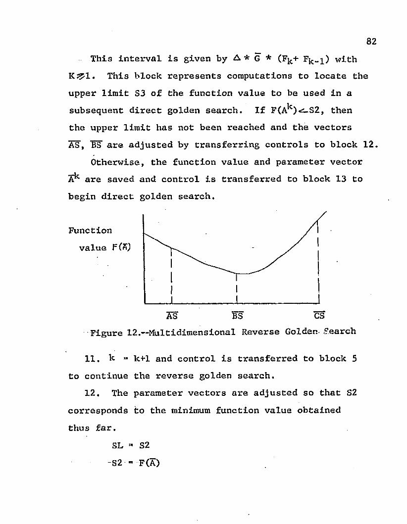
82This interval is given by A * G * (**k+ ^k^) with

K^l. This block represents computations to locate the upper limit S3 of the function value to be used in a subsequent direct golden search. If F(A^)<i-S2, then the upper limit has not been reached and the vectors 3£s, Is are adjusted by transferring controls to block 12.

Otherwise, the function value and parameter vector are saved and control is transferred to block 13 to

begin direct golden search.

Functionvalue

CSIsASFigure 12.— Multidimensional Reverse Golden-Search

11. k =» k +1 and control is transferred to block 5 to continue the reverse golden search.

12, The parameter vectors are adjusted so that S2 corresponds to the minimum function value obtained thus far.

SL a S2 -S2-- F(A)

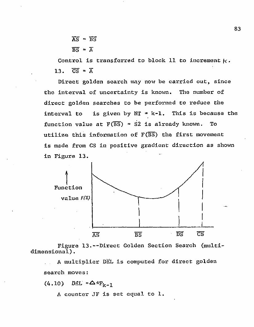
Control is transferred to block 11 to increment /<.13. CS » ADirect golden search may now be carried out, since

the interval of uncertainty is known. The number of direct golden searches to be performed to reduce the interval to is given by NT 31 k-1. This is because the function value at F(BS) = S2 is already known. To utilize this information of F(BS) the first movement is made from CS in positive gradient direction as shown in Figure 13.

Function

BS DS CSASFigure 13.--Direct Golden Section Search (multi­

dimensional) .A multiplier DEL is computed for direct golden

search moves:(4.10) DEL

A counter JF is set equal to 1.

84

14. A new parameter vector A is generated accordingto:(4.11) A 51 CS + DEL * G

In case, all the parameter range constraints are violated, the lowest function value S2 and the associated parameter vector BS are returned to calling program by transferring control to point f.

Otherwise the current parameter vector is saved in location X)5i and SUM2 is set equal to F (A).

15. A check is made to determine whether the numbers of iterations required for direct golden search are complete or not. JF=NT signifies end of direct golden search and to determine the minimum value of the function within an accuracy of A , in parameter values, controlis transferred to block 17.

16. If JF is not equal to NX, direct golden searchproceeds. JF is incremented by 1 and k reduced by 1 tosignify completion of a direct iteration step.

A new DEL value is computed for use in futureiteration and control is transferred to block 18.

17. Apparent minima within an accuracy of A has been located. The values SUM2 and S2 are compared so that the lower of the two may be chosen to return to the calling program.

85

18. If SUM 2^S2, then the CS vector Is modified (this follows from assumption of unimodality in the present negative gradient direction).

CS - DSDS " BSXU =* TJsF(AO) - S2

Control is transferred to .block 20,19. If SUM 2<£. S2 then the AS vector is modified,

since the minima cannot lie in the region between Xs and BS due to assumption of unimodality.

AS - BSS3 - mS2 =* SUM2F(XO) - S2

Control is returned to block 14.20. A move is made in the negative gradient direction

from the AS vector.X - - DEL * G X - XS + XSUM2 a S2

In case all range constraints are violated, control is returned to point f.

86

21. The function value at F(A) is saved in location S2 and the BS vector takes on the values of current parameter vector A. Control is returned to point ra.

Continued PARTANAn information flow diagram (Figure 14) describes the

application of Continued PARTAN to a minimization problem.The steps are:

1. Starting at the initial point AO, the search is conducted in the negative gradient direction until a minimum point AT in this direction is found.

2. The parameter value AT is saved and the gradient at AT is computed.

A search is made in the negative gradient direction (at ST) until the point A2* is located.

A - 5Z3. The general iteration step begins here. Initially

R is given by AR - AO. A search is made in R direction „ oto locate the new point A. This corresponds to A .

The storage vectors are adjusted so that now contains and AT contains4. If the number of iterations equal 2*N-1, the

, icomputations are terminated; otherwise, a search is made in the negative gradient direction to locate point

(N is the number of unknown parameters.)2? ** A4

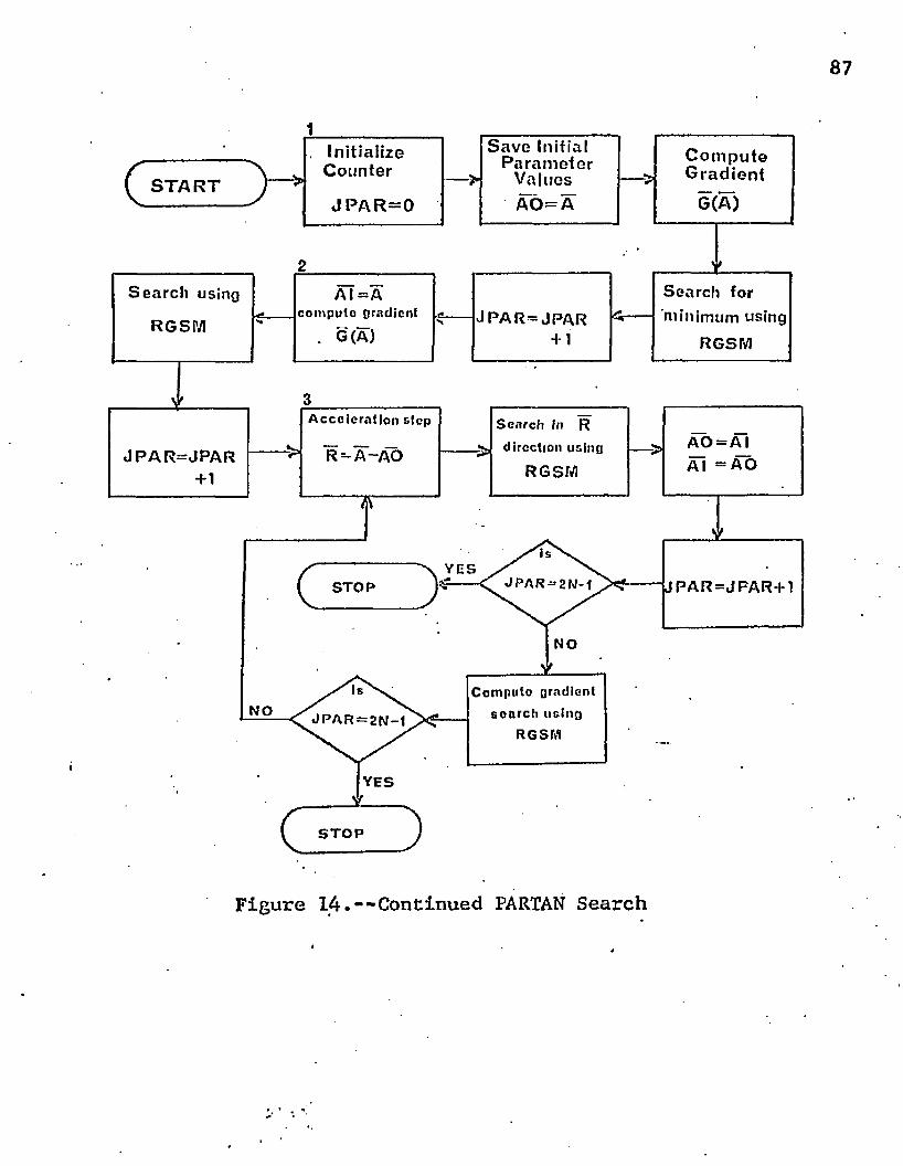
^ S T A R T ^ — *

. In itia lize Counter — >

Save Initial Parameter

Values -->Com puteG radient

J P A R = 0 A O = A G(A)

Search using

R G S M

A I = Acompulo gradient

. G (A)J P A R ~ J P A R

+ 1

Search for

minimum using

RGSM

Acceleration step Search fn R

J P A R =JP A R + 1

—- _ direction using

RGSM— 5> AO = A 1

R —A —AO A l = A O

C YES <C JPAR = 2N-1 JP A R = JP A R + 1

is

J PAR — 2N-1

Compulo gradient search using

RGSM

Figure 14.— Continued PARTAN Search

88

5. A check is made to note if the specified number of iterations have been carried out. In case more iterations are required, control is transferred to step 3.

The one-dimensional searches at various steps in the method have been carried out using the three separate interpolation schemes--QUAD, RGSM, and PIS. In Chapter V description of the results obtained and comparison of the efficiencies of the three interpolation schemes as applied with continued PARTAN to the DEPI problem are given.

SummaryThe computational details of the various optimization

techniques discussed in Chapter III have been elucidated in this chapter. Flow-charts describing computer implementation of these techniques have been developed as a part of this study. This facilitates development of the OMA far DEPI problems as discussed in Chapter V.

CHAPTER V

DEVELOPMENT OF OPTIMUM MINIMIZATION ALGORITHM (OMA) FOR THE

DEPI PROBLEM

IntroductionThis chapter is concerned with the development of

OMA based on the methods discussed and programmed in earlier chapters. The development is based on utilizing information from known differential equation forms and applying these in conjunction with the various minimization methods (Chapters III and IV). In the following details of the principle used toward this end are given.

General CommentsIn Chapter III, it was shown that several

optimization techniques are applicable to the least square estimation of the DEPI problem. However, these techniques have not previously been applied comparatively to such problems. It was observed upon application of these procedures to the problem at hand that the efficiencies of some of the methods were very different from those in literature.^6,92 Because of this an "Optimum Minimization Algorithm" (OMA) was deemed desirable combining the best features of the known minimization techniques.

89

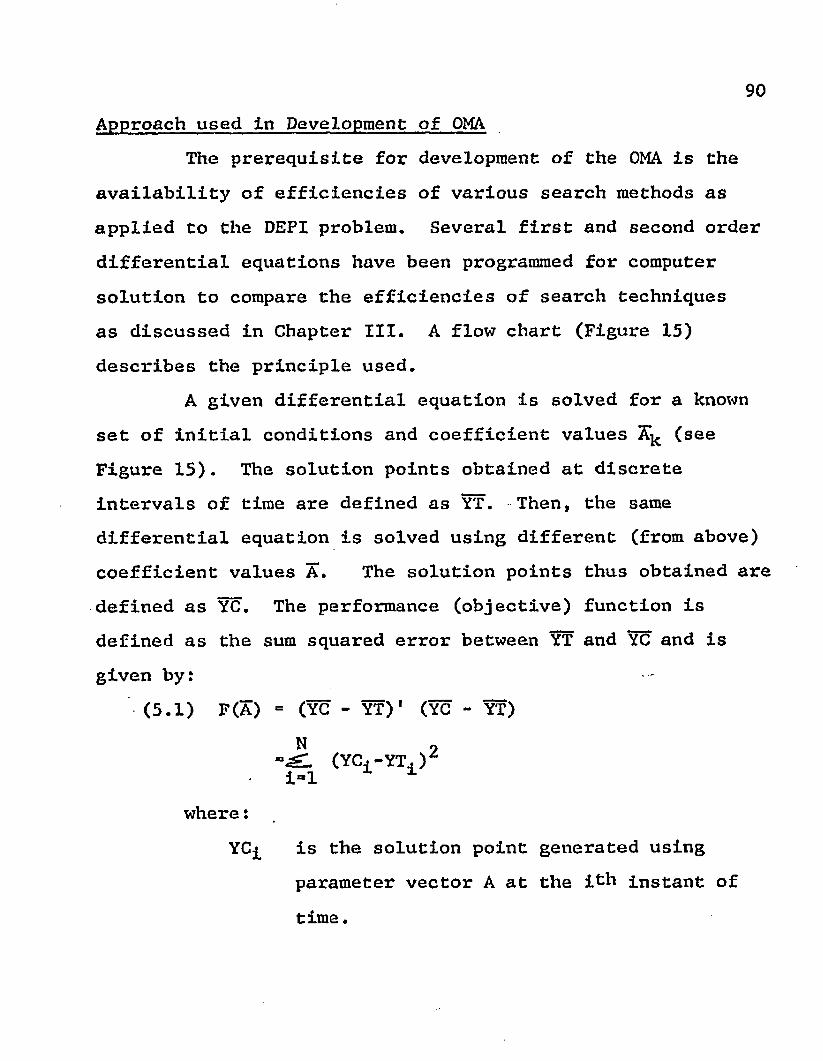
90Approach used In Development of OMA

The prerequisite for development of the OMA is the availability of efficiencies of various search methods as applied to the DEPI problem. Several first and second order differential equations have been programmed for computer solution to compare the efficiencies of search techniques as discussed in Chapter III. A flow chart (Figure 15) describes the principle used.

A given differential equation is solved for a known set of initial conditions and coefficient values (see Figure 15). The solution points obtained at discrete intervals of time are defined as YT. Then, the same differential equation is solved using different (from above) coefficient values A. The solution points thus obtained are defined as YC. The performance (objective) function Is defined as the sum squared error between ¥t and Y(J and is given by:

(5.1) F(A) = (YC - YT)1 (YC - YT)N 2 (YCi-YTj)i»l 1

where:YC^ is the solution point generated using

parameter vector A at the ith instant of time.

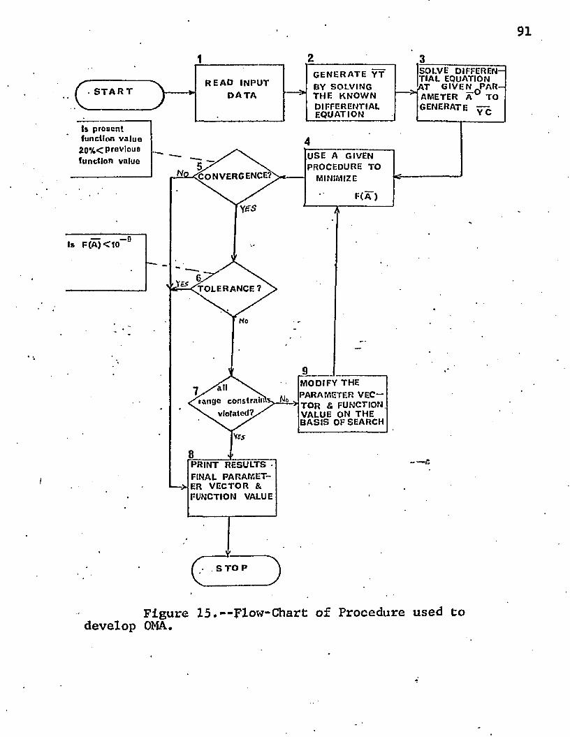
. S T A R T >

Is present function value20%< Pilousfunction value

. -9Is F (A) < 10

tio

fi

— >

[CONVERGENCE?

' / a l l N . range constraint^N* \. violated?/

^<TOLERANCE?

MODIFY THE PARAMETER VEC­TOR & FUNCTION. VALUE ON THE BASIS OF SEARCH

PRINT RESULTS •FINAL PARAMET­ER VECTOR & FUNCTION VALUE

R EAD INPUT D A T A

GENERATE YTBY SOLVING THE KNOWNDIFFERENTIALEQUATION

USE A GIVEN PROCEDURE TO

MINIMIZE

SOLVE DIFFEREN­TIAL EQUATION AT G IV E N -P A R ­AMETER A TO GENERATE

Figure 15.--Flow-Chart of Procedure used to develop OMA.

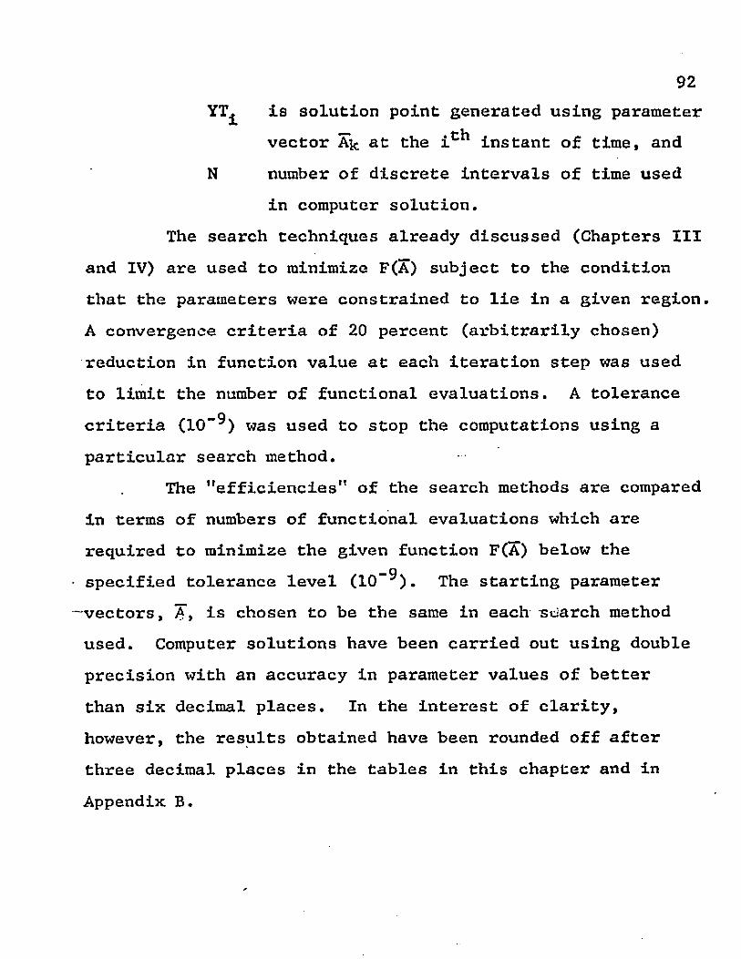
92

YT^ is solution point generated using parameter— fhvector at the i instant of time, and

N number of discrete intervals of time used in computer solution.

The search techniques already discussed (Chapters III and IV) are used to minimize F(A) subject to the condition that the parameters were constrained to lie in a given region. A convergence criteria of 20 percent (arbitrarily chosen) reduction in function value at each iteration step was used to limit the number of functional evaluations. A tolerance criteria (10** ) was used to stop the computations using a particular search method.

The "efficiencies" of the search methods are compared in terms of numbers of functional evaluations which are required to minimize the given function F(A) below the

• specified tolerance level (10”^). The starting parameter —vectors, is chosen to be the same in each ^ciarch method used. Computer solutions have been carried out using double precision with an accuracy in parameter values of better than six decimal places. In the Interest of clarity, however, the results obtained have been rounded off after three decimal places in the tables in this chapter and in Appendix B.

93First Order Differential Equation

The following first order differential equation is used to generate the data points YT.

( 5 * 2 ) Ht + y a 1'° O e t ^ O . 5y(0) = 0.0

YTf * where y^ is the value obtained at thei*-*1 instant of time.

To generate YC the differential equation (5.3) is solved.

<5*3> a2 + Ai y = 1,0 0 - * - o *5y(0) » 0

where: YC^ a y^ andA- and A2 are arbitrarily chosen starting parameter values.

84Creeping Random Search (See Appendix 0 for details)Table 1 shows the results of application of Creeping

Random Method to objective function, Equation (1).The initial parameter vector was chosen as (1.2,

1.2). The objective function corresponding to this vectorF(A°) was 2.824*10"2 .

As can be discerned from Table 1, the random searchin trial 1, when the entire permissible region is used forsearching, produced no improvement in function value. This

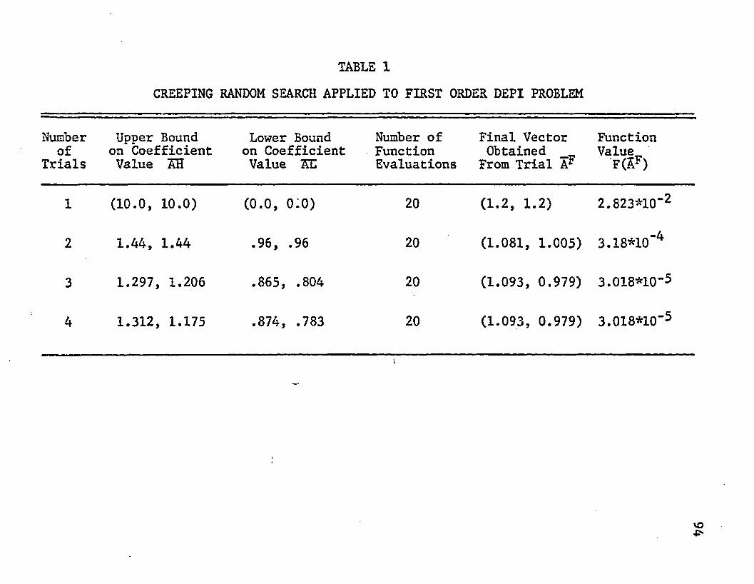
TABLE 1CREEPING RANDOM SEARCH APPLIED TO FIRST ORDER DEPI PROBLEM

Numberof

TrialsUpper Bound on Coefficient Value EH

Lower Bound on Coefficient Value EE

Number ofFunctionEvaluations

Final Vector Obtained

From Trial A^FunctionValue

F(£?)

1 (10.0, 10.0) (o.o, o;o) 20 (1.2, 1.2) 2.823*10"2

2 1.44, 1.44 .96, .96 20 (1.081, 1.005) 3.18*10"4

3 1.297, 1.206 .865, .804 20 (1.093, 0.979) 3.018*10"5

4 1.312, 1.175 .874, .783 20 (1.093, 0.979) 3.018*10'5

vO

95finding is true in 10 out of 17 (P' 50%) independent attempts at minimization starting from (1.2, 1.2) (See Appendix B, Table 1). At trial 2, the permissible range of coefficient values is shrunk to + 20% around (1.2, 1.2). A significant improvement in the objective function value F(A) is observed with random searching in this region. A further improvement in objective function is obtained when the permissible region of parameter values was shrunk around the current estimate A (1.081, 1.005) at the end of trail 2. The search at step 4 resulted in no further improvement in objective function value. This suggested that a random low objective function value has been located at (1.095, 0.979) within the region given by:

AH - (1.297, 1.206)ST =» (1.874, .783)The objective function value at (1.093, 0.979) is

3.018*10“^ and, therefore, a significant improvement over the initial function value of 2.824*10 . However, theCreeping Random Method failed to converge to the true coefficient values (1.0, 1.0). It is quite possible that an increased number of functional evaluations at each trial step may result in a better estimate of coefficient values.As the number of unknown parameters is increased, the efficiency of the Creeping Random Search on the average decreased (Appendix B, Table 3).

96While the Creeping Random Search did yield lower

function values F(£), the average numbers of functional evaluations required were rather large, on the average greater than 100 (Appendix B, Table 1). Table 2, Appendix B summarizes the results of Creeping Random Search applied at various initial parameter values. As may be observed, the average number of required functional evaluations are greater than 100 for a given initial parameter value.

However, due to vastness of the parameter space, there must be a way to choose the starting parameter vector in the absence of a priori knowledge of the approximate values of the true parameter vector. It is felt that the Random Search may be employed in this capacity, since it provides unbiased parameter vectors.

Once the starting parameter vector has been determined, more powerful methods may be used for function minimization. Random Search is also used to conduct a search around the final optimum value to assure one that no false optimum has been attained.

Pattern SearchThe pattern search was carried out using .001 as

the parameter change magnitude, EPS, in the exploratory moves. The number of functional evaluations on the average increased as the parameter change magnitudes were reduced

(See Tables 4 and 5, Appendix B.)

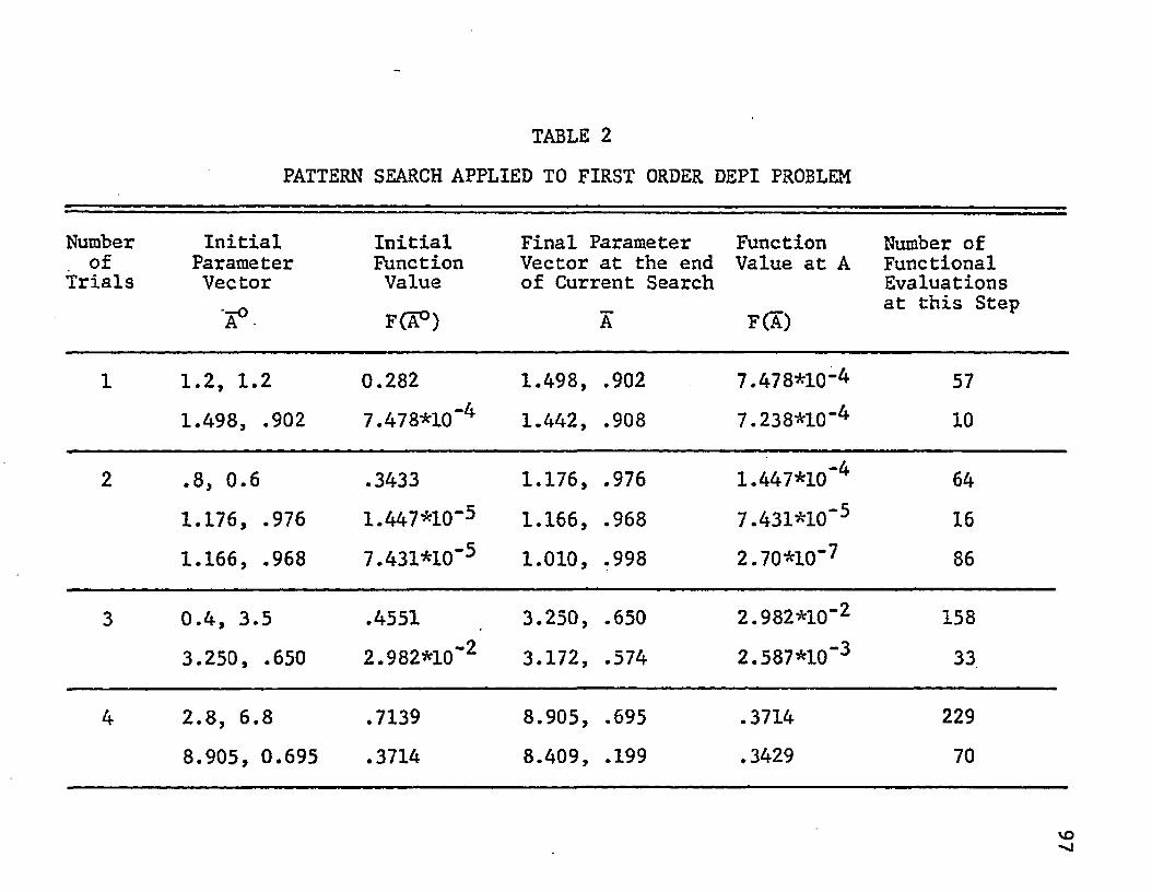
TABLE 2PATTERN SEARCH APPLIED TO FIRST ORDER DEPI PROBLEM

Numberof

TrialsInitial

ParameterVector

A°

InitialFunctionValueF(A°)

Final Parameter Vector at the end of Current Search

A

Function Value at A

F(A)

Number of Functional Evaluations at this Step

1 1.2, 1.2 0.282 1.498, .902 7.478*10"4 571.498, .902 7.478*10"4 1.442, .908 7.238*10“4 10

2 .8, 0.6 .3433 1.176, .976 1.447*10*4 641.176, .976 1.447*10 1.166, .968 7.431*10“** 161.166, .968 7.431*10”** 1.010, .998 2.70*10”7 86

3 0.4, 3.5 .4551 3.250, .650 2.982*10"2 1583.250, .650 2.982*10"2 3.172, .574 2.587*10"3 33

4 2.8, 6.8 .7139 8.905, .695 .3714 2298.905, 0.695 .3714 8.409, .199 .3429 70

98It was surprising to note that the application of

pattern search did not consistently meet the convergence criteria, thereby necessitating the termination of search. This may be due to the fact that the objective function does not change considerably with small changes in the parameter values from a given parameter vector. The trial conducted from the initial parameters vector (0 .8, 0 .6) converged to (1.010, 0.998) with a function value of 2.7*10"^. This is the only successful search using this technique. With all other initial parameter vectors, there is very little improvement in the function value compared with the number of functional evaluations that are required.

In order to study the effects of the magnitude of exploratory moves; i.e., EPS, on the number of functional evaluations another run has been made with the bigger exploratory moves. The search in this variation is begun with EPS^O.l. At the next iteration step, Xtfhen> the exploration in current pattern search failed, EPS is reduced to .01. The final iteration is carried out using EPS=*.001.

While the number of functional evaluations decreased in this variation (see Tables 4 and 5, Appendix B), convergence of pattern search is still rather poor compared ..to the LSMM.

Discrete Steepest Descent SearchThis search requires explicit computation of gradient

of the criteria function at each iteration step. Three one­dimensional search methods were compared in order to determine which procedure computed the optimal distance that could be traversed in the negative gradient direction with the lowest number of functional evaluation.

Table 3 describes the results of application of the three one-dimensional searches to the objective function equation (1). The movements in each case were in the negative gradient direction from the same starting parameter vectors. Comparisons were made with several different starting parameter values.

As can be seen in Table 3, the quadratic inter­polation method yielded the best strategy since in each case it required the least number of functional evaluations -for the greatest reduction in function value.

Table 4 summarizes the results obtained by using RGSM at the various iteration steps in the discrete steepest descent search. The searches were conducted from several different starting parameter vectors. The required accuracy in parameters was varied and a comparison was made among the numbers of required functional evaluations with each used. As can be seen (Table 4) the number of functional

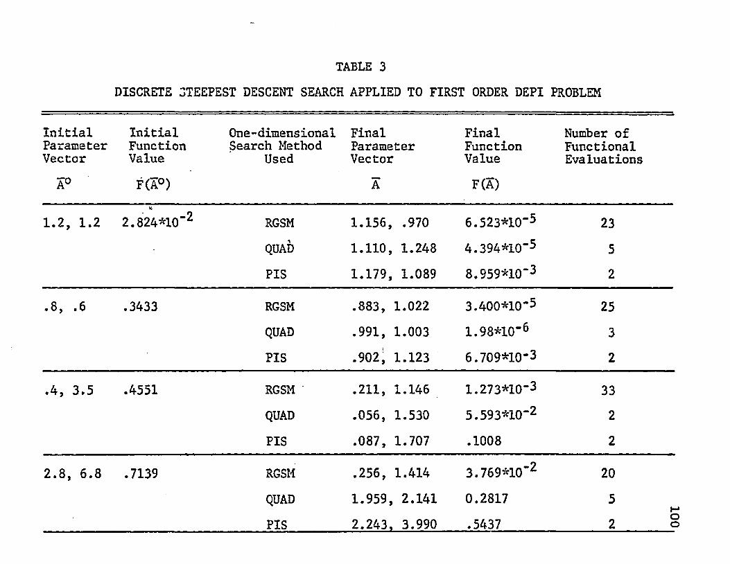
TABLE 3DISCRETE STEEPEST DESCENT SEARCH APPLIED TO FIRST ORDER DEPI PROBLEM

Initial Initial One-dimensional Final Final Number ofParameter Function Search Method Parameter Function FunctionalVector Value Used Vector Value EvaluationsA0 F(A°) A F(A)

1.2, 1.2 2.824*10‘2 RGSM 1.156, .970 6.523*10“5 23QUAD 1.110, 1.248 4.394*10-5 5PIS 1.179, 1.089 8.959*10“3 2

.8, .6 .3433 RGSM .883, 1.022 3.400*10"5 25QUAD .991, 1.003 1.98*10"6 3PIS .902^ 1.123 6.709*10*3 2

.4, 3.5 .4551 RGSM .211, 1.146 1.273*10“3 33QUAD .056, 1.530 5.593*10‘2 2PIS .087, 1.707 .1008 2

2.8, 6.8 .7139 RGSM .256, 1.414 3.769*10"2 20QUAD 1.959, 2.141 0.2817 5

__________________________ PIS_________2.243. 3.990 .5437_______________2

100

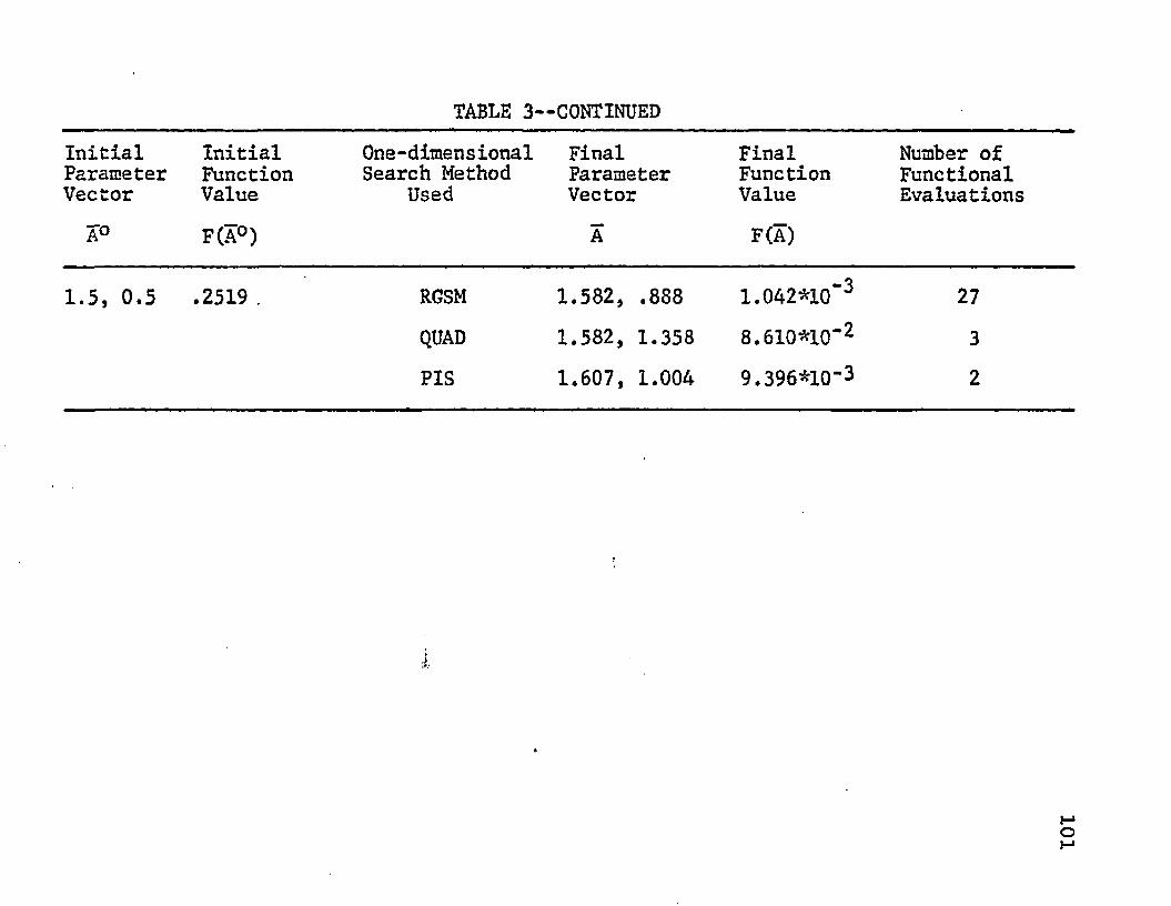
TABLE 3— CONTINUEDInitialParameterVector

A°

InitialFunctionValueF(A°)

One-dimensional Search Method

UsedFinalParameterVectorA

FinalFunctionValueF(A)

Number ofFunctionalEvaluations

1.5, 0.5 .2519 . RGSM 1.582, .888 1.042*10“3 27QUAD 1.582, 1.358 8.610 *10"^ 3PIS 1.607, 1.004 9.396*10-3 2

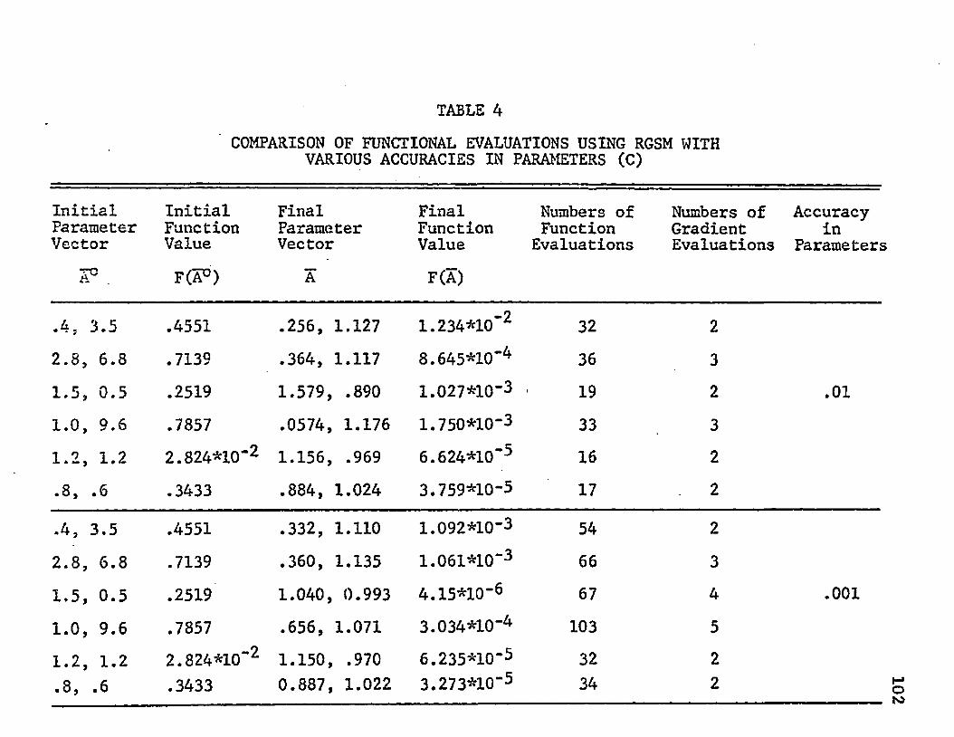
TABLE 4COMPARISON OF FUNCTIONAL EVALUATIONS USING RGSM WITH

VARIOUS ACCURACIES IN PARAMETERS (C)

InitialParameterVector

InitialFunctionValue

FinalParameterVector

FinalFunctionValue

Numbers of Function Evaluations

Numbers ofGradientEvaluations

Accuracyin

ParametersA° . F(A°) A F(A)

A, 3.5 .4551 .256, 1.127 1.234*10”2 32 22.8, 6.8 .7139 .364, 1.117 8.645*10~4 36 31.5, 0.5 .2519 1.579, .890 1.027*10’3 19 2 .011.0, 9.6 .7857 .0574, 1.176 1.750*10‘3 33 31.2, 1.2 2.824*10“2 1.156, .969 6.624*10’5 16 2

.8, .6 .3433 .884, 1.024 3.759*10-5 17 2

.4, 3.5 .4551 .332, 1.110 1.092*10-3 54 2

2.8, 6.8 .7139 .360, 1.135 1.061*10“3 66 31.5, 0.5 .2519 1.040, 0.993 4.15*10-6 67 4 .001

1.0, 9.6 .7857 .656, 1.071 3.034*10"4 103 51.2, 1.2 2.824*10"2 1.150, .970 6.235*10*5 32 2.8, .6 .3433 0.887, 1.022 3.273*10“5 34 2 102

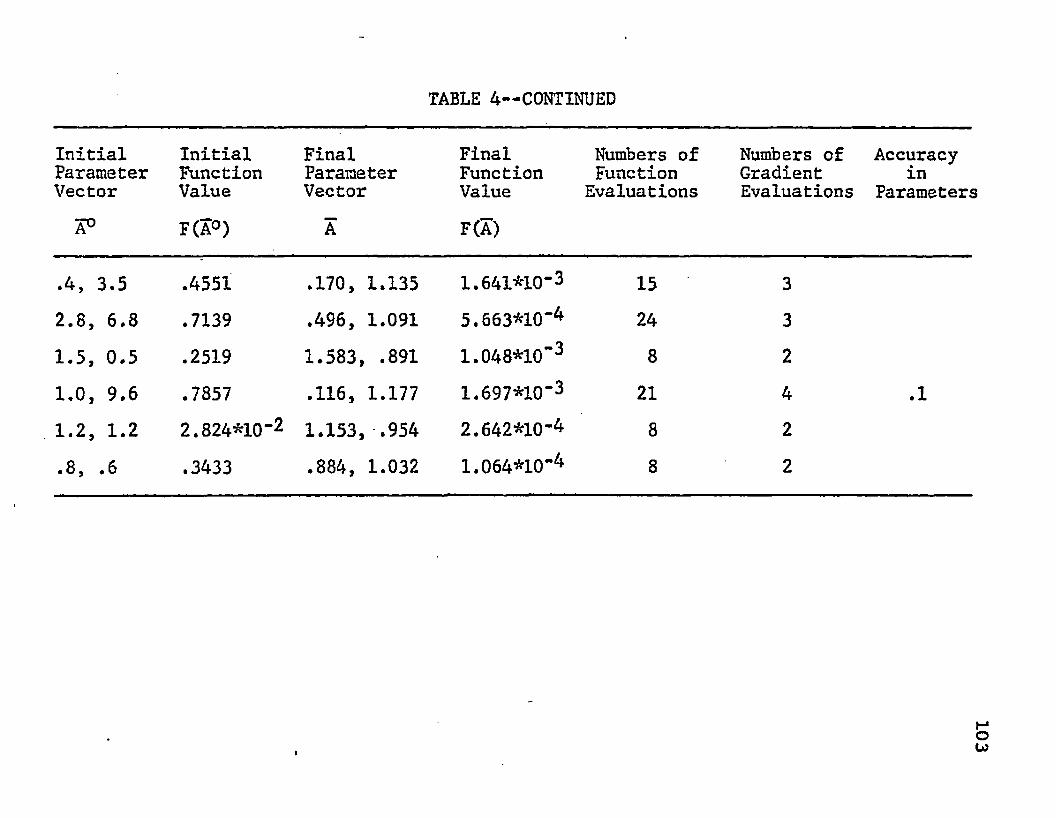
TABLE 4— CONTINUED

InitialParameterVectorA0

InitialFunctionValueF(A°)

FinalParameterVector

A

FinalFunctionValueF(A)

Numbers of Function Evaluations

Numbers ofGradientEvaluations

Accuracyin

Parameters

.4, 3.5 .4551 .170, 1.135 1.641*10-3 15 32.8, 6.8 .7139 .496, 1.091 5.663*10*4 24 31.5, 0.5 .2519 1.583, .891 1.048*10"3 8 2

1.0, 9.6 .7857 .116, 1.177 1.697*10'3 21 4 .11.2, 1.2 2.824*10-2 1.153, .954 2.642*10-4 8 2

.8, .6 .3433 .884, 1.032 1.064*10*4 8 2

103

104evaluation at any given iteration step were lowest with Ca0.1. The convergence of these methods was rather poor (none converged to the true values (1.0, 1.0)). It was felt that the discrete steepest descent could be used only at the initial parameter vectors for a rough approximation of the true parameter vector.

A detailed description of RGSM described in Tables 3 and 4 has been provided in Appendix B (Tables 7, 8, 9).Table 10 (Appendix B) contains detailed description of quadratic interpolation as applied to the first order DEPI problem. As the parameter values approach the true vector (1.0 , 1.0) characterized by a lower function value, the number of functional evaluations required by quadratic interpolation on an average increased.

Comparison of Other Hlnimization Method's Developed in Chapters III and-1 IV

Various authors have determined that the Fletcher- Powell method is superior for a general function minimization. Other workers have felt that continued PARTAN, since it takes into account the geometrical features of the function, provides the best strategy. In the particular case of DEPI problem, since an approximation to the second order derivatives was available, the LSMM scheme has been found the most efficient (see Table 5).

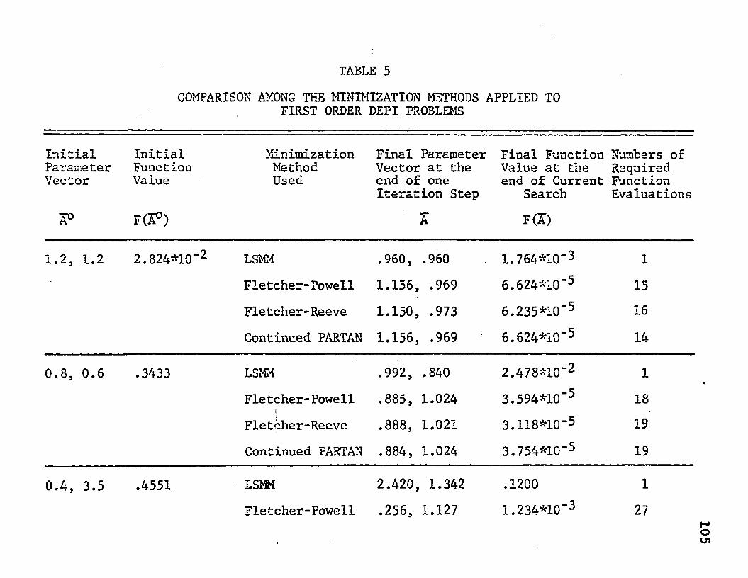
TABLE 5COMPARISON AMONG THE MINIMIZATION METHODS APPLIED TO

FIRST ORDER DEPI PROBLEMS

InitialParameterVector

InitialFunctionValue

MinimizationMethodUsed

Final Parameter Vector at the end of one Iteration Step

Final Function Value at the end of Current

Search

Numbers of Required Function Evaluations

A0 F(A°) A F(A)

1.2, 1.2 2.824*10~2 LSMM .960, .960 1.764*10’3 1Fletcher-Powell 1.156, .969 6.624*10"5 15Fletcher-Reeve 1.150, .973 6.235*10“5 16Continued PARTAN 1.156, .969 ‘ 6.624*10“3 14

0 .8, 0.6 .3433 LSMM .992, .840 2.478*10‘2 1Fletcher-Powell .885, 1.024 3.594*10”'* 18

iFletcher-Reeve .888, 1.021 3.118*10"5 19Continued PARTAN .884, 1.024 3.754*10’5 19

0.4, 3.5 .4551 ■ LSMM 2.420, 1.342 .1200 1

Fletcher-Powell .256, 1.127 1.234*10"3 27 105

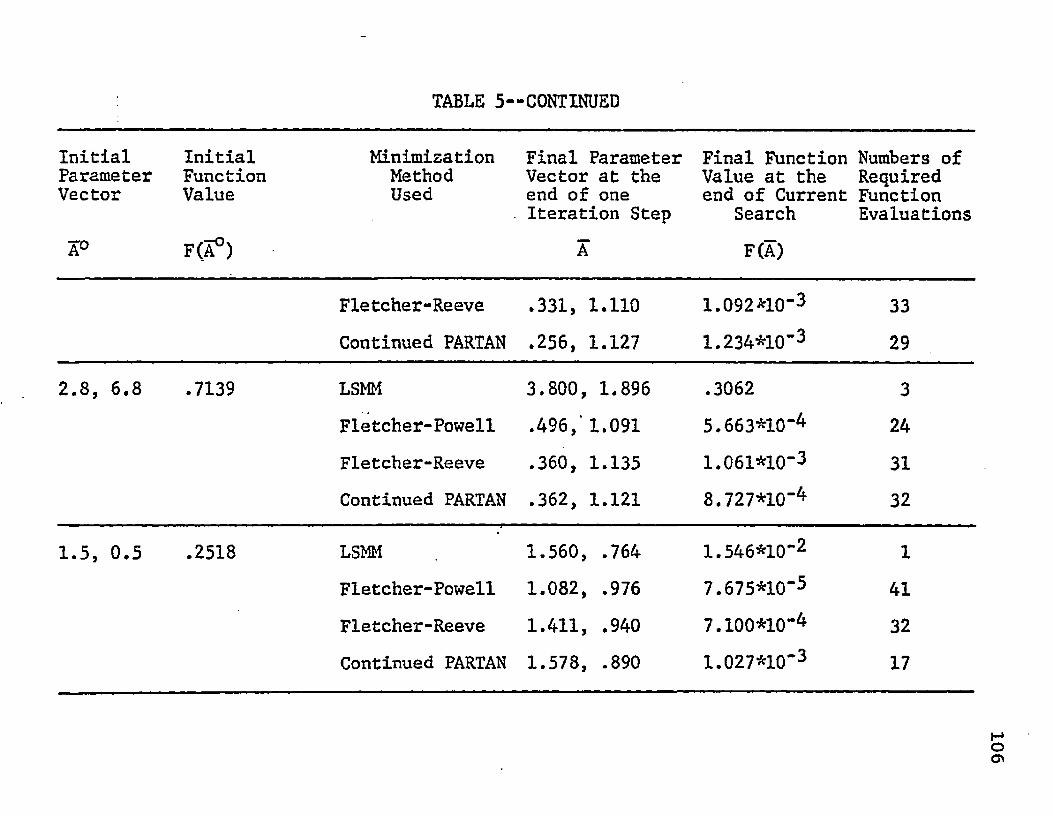
TABLE 5— CONTINUED

InitialParameterVector

InitialFunctionValue

MinimizationMethodUsed

Final Parameter Vector at the end of one Iteration Step

Final Function Value at the end of Current

Search

Numbers of Required Function Evaluations

A0 F(A°) A F(A)

Fletcher-Reeve .331, 1.110 1.092*10"3 33Continued PARTAN .256, 1.127 1.234*10"3 29

2.8, 6.8 .7139 LSMM 3.800, 1.896 .3062 3Fletcher-Powell .496, 1.091 5.663*10-4 24Fletcher-Reeve .360, 1.135 1.061*10“3 31Continued PARTAN .362, 1.121 8.727*10“4 32

1.5, 0.5 .2518 LSMM 1.560, .764 1.546*10“2 1Fletcher-Powell 1.082, .976 7.675*10“5 41Fletcher-Reeve 1.411, .940 7.100*10"4 32Continued PARTAN 1.578, .890 1.027*10"3 17

106

107Table 5 shows a comparison between the following

minimization schemes:1. Least Square Minimization Method2. Fletcher-Powell Method----/Using RGSM for3. Fletcher-Reeve Method A one-dimensionalA. Continued PARTAN searchesThe results are compared on the basis of completion

of an iteration step as applied to a particular method.Thus, it could be seen that in the case of first

order DEPI problems LSMM provided the best strategy for reduction in the value of performance function. Table 6, Appendix B, details the excellent convergence properties of the LSMM.

As can be discerned from above, the LSMM converged to the true parameter vector A 3 (1,1) for all the different starting parameter vectors used (Table 6, Appendix B). It is also observed that the number of functional evaluations required at every iteration step were lowest among the search methods used in this dissertation.

This led us to a discussion of minimization methods applied to second order DEPI problems. This is necessary in order to study the effect of increased number of .parameters on the various search techniques.

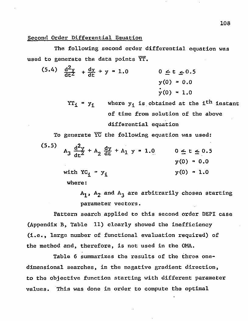
108

Second Order Differential EquationThe following second order differential equation was

used to generate the data points W .(5.4) d£v + | 3 r + y - 1.0 0 1 e.0.5dtz dt — —

y(0) * 0.0 y(0) « 1.0

YT^ ** y^ where y^ is obtained at the i*1*1 instant of time from solution of the above differential equation

To generate YC the following equation was used:

d^v dvA^ + 2 d? ^1 y “ ^*0 0 ^ t ^-0.5y(0) » 0.0

with YC^ " y^ y(0) * 1.0where:

A^, A2 and A^ are arbitrarily chosen starting parameter vectors.

Pattern search applied to this second order DEPI case (Appendix B, Table 11) clearly showed the inefficiency (i.e., large number of functional evaluation required) of the method and, therefore, is not used in the OMA.

Table 6 summarizes the results of the three one­dimensional searches, in the negative gradient direction, to the objective function starting with different parameter values. This was done in order to compute the optimal

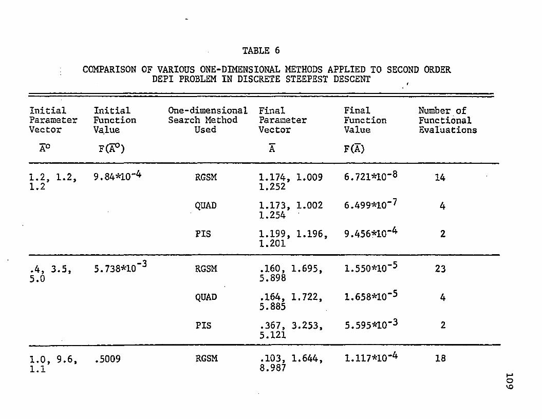
TABLE 6COMPARISON OF VARIOUS ONE-DIMENSIONAL METHODS APPLIED TO SECOND ORDER

DEPI PROBLEM IN DISCRETE STEEPEST DESCENT

InitialParameterVector

InitialFunctionValue

One-dimensional Search Method

UsedFinalParameterVector

FinalFunctionValue

Number ofFunctionalEvaluations

A° F(A°) A F(A)

1.2, 1.2, 1.2

9.84*10“4 RGSM 1.174, 1.009 1.252

6.721*10“8 14

QUAD 1.173, 1.002 1.254

6.499*10“7 4

PIS 1.199, 1.196, 1.201

9.456*10“4 2

.4, 3.5,5.0

5.738*10“3 RGSM .160, 1.695, 5.898

1.550*10“-* 23

QUAD .164, 1.722, 5.885

1.658*10“5 4

PIS .367, 3.253, 5.121

5.595 *10 2

1.0, 9.6,1.1

.5009 RGSM .103, 1.644, 8.987

1.117*10"4 18

109

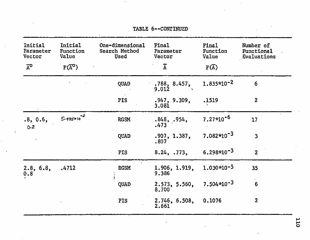
TABLE 6— CONTINUED

InitialParameterVector

InitialFunctionValue

One-dimensional Search Method

UsedFinalParameterVector

FinalFunctionValue

Number ofFunctionalEvaluations

A0 F(A°) A F(A)

■ QUAD .788, 8.457, 9.012

1.835*10-2 6

PIS .947, 9.309, 3.081

.1519 2

*8, 0 .6, 0*2

^ -2 5-43S*H> RGSM .848, .954, .473

7.27*10“6 17

■QUAD .907, 1.387,

.8077.082*10‘3 3

PIS 8.24, .773, 6.298*10"3 2

2.8, 6.8, 0.8

.4712 RGSMi

j1.906, 1.919, 9.386

1.030*10-5 35

QUAD 2.573, 5.560, 8.700

7.504*10~3 6

■ PIS 2.746, 6.508, 2.661

0.1076 2

110

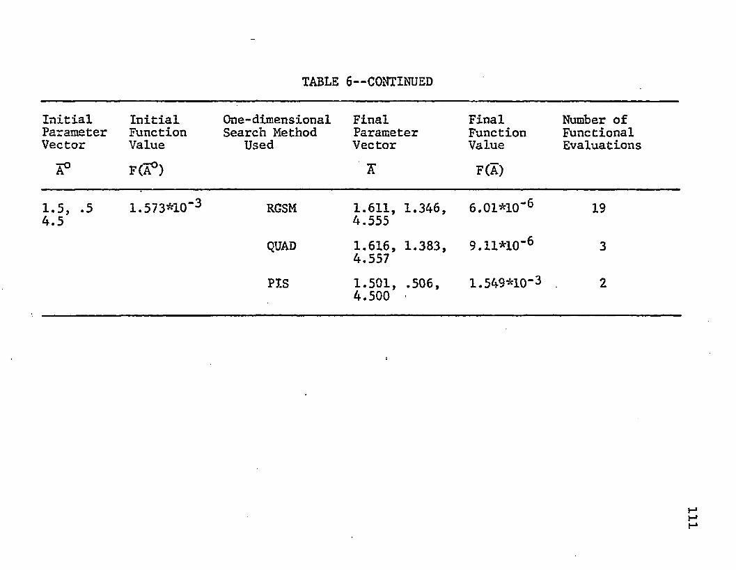
TABLE 6— CONTINUED

InitialParameterVector

InitialFunctionValue

One-dimensional Search Method

UsedFinalParameterVector

FinalFunctionValue

Number ofFunctionalEvaluations

A° F(A°) £ F(A)

1.5, .5 4.5

1.573*10"3 RGSM 1.611,4.555

1.346, 6.01*10“6 19

QUAD 1.616,4.557

1.383, 9.11*10-6 3

PIS 1.501,4.500

.506, 1.549*10“3 2

111

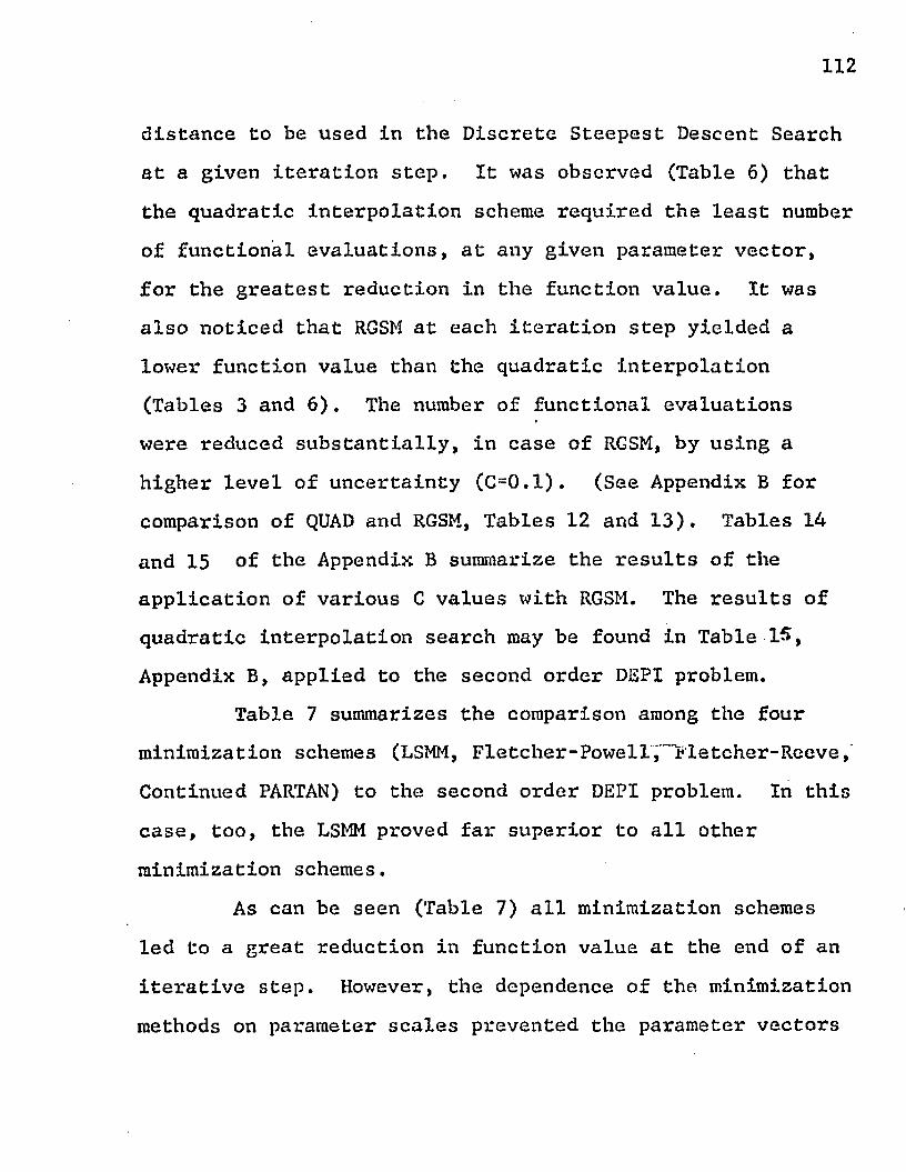
112

distance to be used in the Discrete Steepest Descent Search at a given iteration step. It was observed (Table 6) that the quadratic interpolation scheme required the least number of functional evaluations, at any given parameter vector, for the greatest reduction in the function value. It was also noticed that RGSM at each iteration step yielded a lower function value than the quadratic interpolation (Tables 3 and 6). The number of functional evaluations were reduced substantially, in case of RGSM, by using a higher level of uncertainty (C=0.1). (See Appendix B for comparison of QUAD and RGSM, Tables 12 and 13). Tables 14 and 15 of the Appendix B summarize the results of the application of various C values with RGSM. The results of quadratic interpolation search may be found in Table 15, Appendix B, applied to the second order DEPI problem.

Table 7 summarizes the comparison among the four minimization schemes (LSMM, Fletcher-Powell,""Pietcher-Reeve, Continued PARTAN) to the second order DEPI problem. In this case, too, the LSMM proved far superior to all other minimization schemes.

As can be seen (Table 7) all minimization schemes led to a great reduction in function value at the end of an iterative step. However, the dependence of the minimization methods on parameter scales prevented the parameter vectors

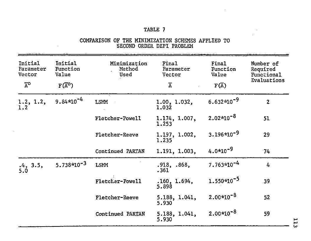
TABLE 7COMPARISON OF THE MINIMIZATION SCHEMES APPLIED TO

SECOND ORDER DEPI PROBLEM

InitialParameterVectorA°

InitialFunctionValueF(A°)

MinimizationMethodUsed

FinalParameterVector

A

FinalFunctionValueF(A)

Number of Required Functional Evaluations

1.2, 1.2, 1.2

9.84*10"4 LSMM 1.00, 1.032, 1.032

6.632*10"9 2

Fletcher-Powell 1.174, 1.007, 1.253

2.02*10“8 51

Fletcher-Reeve 1.197, 1.002, 1.235

3.196*10~9 29

Continued PARTAN 1.191, 1.003, 4.0*10"9 74

.4, 3.5, 5.0

5.738*10“3 LSMM .918, .868, .361

7.763*10~4 4

Fie tcKar-Powel1 .160, 1.694, 5.898

1.550*10”** 39

Fletcher-Reeve 5.188, 1.041, 5.930

2.00*10"8 52

Continued PARTAN 5.188, 1.041, 5.930

2.00*10“8 59 113

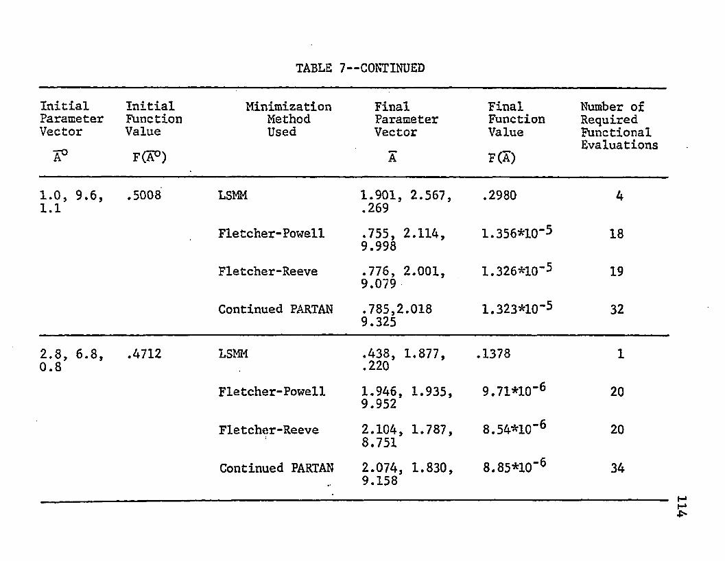
TABLE 7— CONTINUED

InitialParameterVectorA°

InitialFunctionValueF(A°)

MinimizationMethodUsed

FinalParameterVectorA

FinalFunctionValueF(A)

Number of Required Functional Evaluations

1.0, 9.6, 1.1

.5008 LSMM 1.901, 2.567, .269

.2980 4

Fletcher-Powell .755, 2.114, 9.998

1.356*10"5 18

Fletcher-Reeve .776, 2.001, 9.079

1.326*10”-* 19

Continued PARTAN .785,2.0189.325

1.323*10“5 32

2.8, 6.8, 0.8

.4712 LSMM .438, 1.877, .220

.1378 1

Fletcher-Powell 1.946, 1.935, 9.952

9.71*10’6 20

Fletcher-Reeve 2.104, 1.787, 8.751

8.54*10"6 20

Continued PARTAN 2.074, 1.830, 9.158

8.85*10'6 34

114

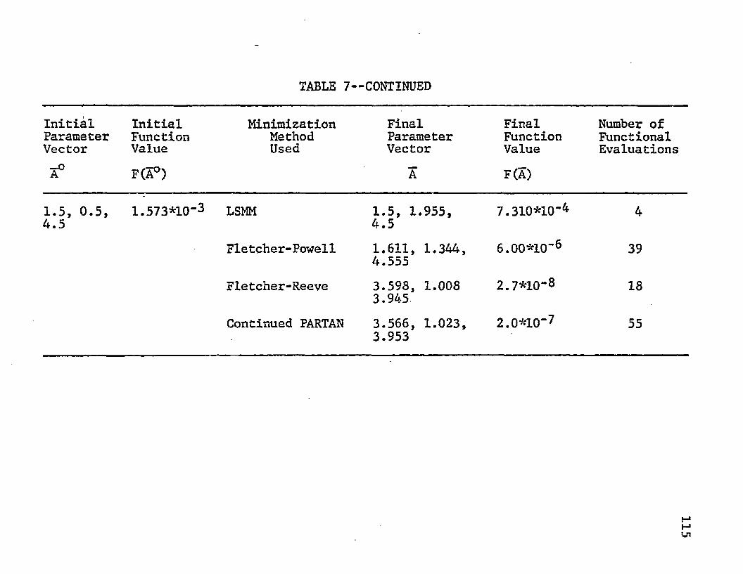
TABLE 7— CONTINUED

InitialParameterVector

InitialFunctionValue

MinimizationMethodUsed

FinalParameterVector

FinalFunctionValue

Number ofFunctionalEvaluations

A° F(A°) A F(A)

1.5, 0.5,4.5

1.573*10”3 LSMM 1.5, 1.955,4.5

7.310*10-4 4

Fletcher-Powell 1.611, 1.344, 4.555

6.00*i0"6 39

Fletcher-Reeve 3.598, 1.008 3.945

2.7*10-8 18

Continued PARTAN 3.566, 1.023, 3.953

2,0*10“7 55

115

116from converging toward the true parameter values (1.0 , 1.0 , 1.0). The second order DEPI problem demonstrates also the multi-modal nature of the objective function F(K).

Detailed inspection of the other minimization methods (Appendix B) showed that these methods were all very efficient in reducing the function value. This was true for the initial stages of the search at any starting param­eter vector. However, as the gradient vector became smaller, indicating closeness of optimum, the convergence of these methods was very poor. By comparison, the LSMM, near the optimum, displayed very good convergence properties. In both the first and second order DEPI problems discussed,LSMM converged to the corresponding true parameter vectors (Appendix B, Table 16), thus displaying its superiority.

Development of the OMAActual experience with the experimentally observed

data shows that LSMM may not result in further reduction of function value even though the gradient magnitude is rather large (see Chapter VII). It has been observed that application of discrete steepest descent at these points led to reduction in function value. Therefore, a discrete steepest descent search is carried out when it is observed that LSMM does not lead to function reduction and gradient magnitudes are large. For large gradient magnitudes

117.

( |g *gI^^IOO) the quadratic interpolation technique has proved very successful, while for smaller gradient magnitudes (100.2 Ig 'g J&^I) the RGSM interpolation has proved very useful. For gradient magnitudes lower than 1, the Greeping Random Search is used to determine the nature of the stationary point. Based on these comments, the OMA developed in this dissertation may be summarized by the flow chart as shown in Figure 16.

Limitations of OMA as Applied to DEPy-probTems

A serious difficulty associated with DEPI problems is that the identification may not be unique. For a parti­cular choice of initial conditions and forcing, it is quite possible that only one particular mode of the system under study is excited. In other words, the solution is determined by one particular root of the system differential equation.When this happens, all other systems possessing this particular mode, under the given condition, will be indistinguishable from each other. F(A) in such cases will approach zero. However, the final parameter vectors A in such cases will have widely different component values.This phenomena was strikingly illustrated in the case ofthe following differential equation:

2(5.6) A3 + a2 (• A]_ y a 1.0 with y(0) a 0, y(0) = 1.0

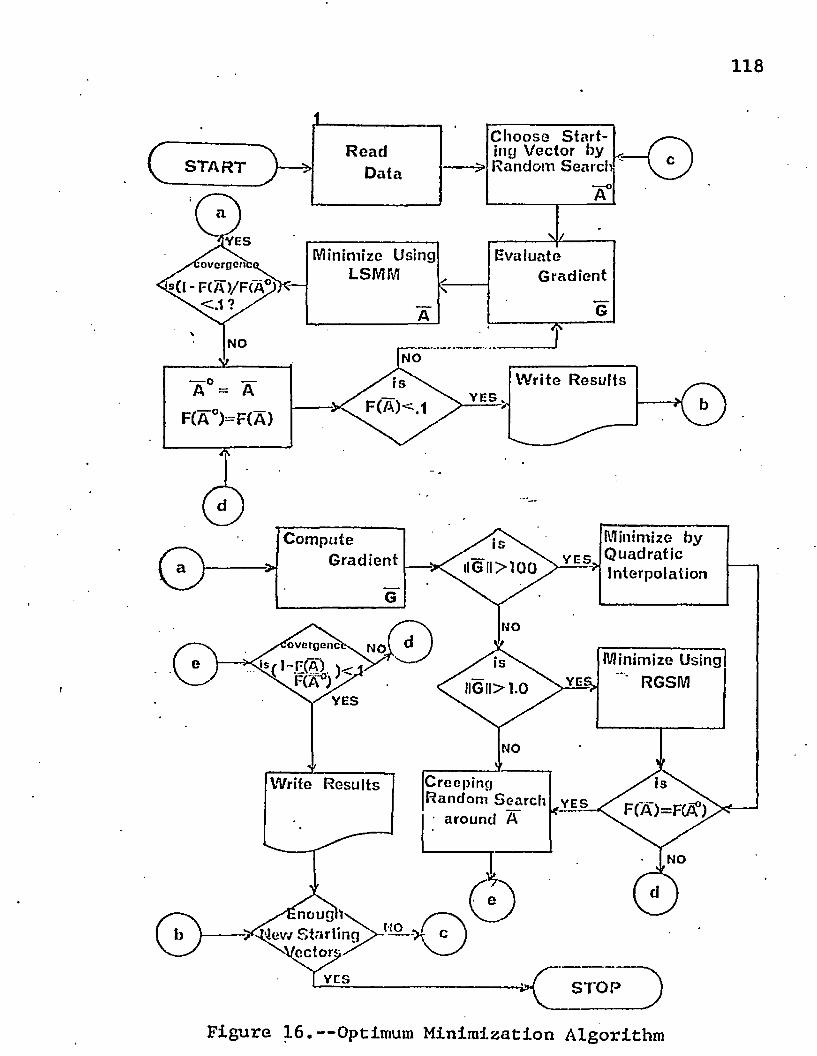
118

Choose S tart­ing Vector by Random Search

ReadDataS T A R T

5yes

C l-F (A )/F (ra^— \ < . 1 ? /

Minimize Using LSM M

EvaluateGradient

NONO

W rite ResultsY E S .

Minimize byQuadraticInterpolation

ComputeGradient YES

NO.✓covergencfc^ n q

^KF(A) )<>"YES

NO

Creeping Random Search ■ around A

Write ResultsYES

NO

✓"Enoughs Jlew S ta rtin g ^ -1— ^ A /c c to rs /^

YES S TO P

Figure 16.--Optimum Minimization Algorithm

119

The true data points YT were generated using the parameter vector A^ (2.0, 3.0, 1.0).

Equation (5.6) was then used for minimization of F(A) and the following starting parameter vector was chosen to generate YC. "K ° (1.0, 1.0, 1.0)

The LSMM scheme resulted in the final parameter vector, Ap, (2.0, 1.4, 0.20), with the resulting F(A)«£ 10“ . which was the absolute convergence criteria.

As may be observed from comparison of Ap with Ap minimization of F(A) did not lead to the same parameter vectors.

An analytic solution of equation (5.6) with parameter vectors given by Ap and *Ap led to the following result:

(5.7) y(t) = 1 (l - e"2t)

Inspection of equation (5.7) pointed out that the particular choice of initial conditions resulted in can­cellation of the root at (*1) with Ap and the root at (+5) with Ap.

A possible approach in such cases may be application of minimization techniques with several different initial conditions and starting vectors. The final parameter vector obtained from each computer run may then be compared against each other in order to identify the true system differential equation.

120The problem of nonuniqueness of the solution may

not arise in the particular case of ventricular diastole model, since the forcing, P(t), used for identification is an arbitrary function of time and several cycles of data are used to define the model. This contention has been borne out by actual experience with experimental data. The analysis of the ventricular model is based on ten consecutive cycles of pressure and diameter data, in diastole, for any given experimental animal used.

Once the structural form of the differential equation has been determined (see Chapter VII) It was tested for uniqueness. When the period of diastole is relatively constant it has been observed that the final parameter vectors obtained using OMA converged to the same values for each cycle of data used. Since the initial conditions (Initial value of the diameter and pressure at the onset of diastole) were different in each cycle and different parameter vectors are chosen for function minimization, it Is quite likely that both possible modes of the proposed second order differential equation are excited. In the absence of "a priori" knowledge of the actual differential equation form it is difficult, however, to assert this contention.

SummaryAn "Optimum Minimization Algorithm" (OMA) has been

developed in this chapter to be used with experimental data for DEPI problems. This development has been based on comparisons of various minimization techniques discussed earlier. The OMA developed is used with the ventricular pressure and diameter data in Chapter VII toward the characterization of the diastolic behavior with a differential equation.

CHAPTER VI EXPERIMENTAL PROCEDURE

The experimental data utilized in developing amathematical model of diastolic behavior of the leftventricle (Chapter VII) were obtained under the expertguidance of Dr. R. L. Hamlin. Dr. Dave Gross, one ofDr. Hamlin's staff cardiologists, assisted with the neededsurgery to obtain the data.

Ten mongrel dogs averaging 20 kg. in body weightwere anesthetized with Fentanyl-droperidol-Pentabarbitalcombination. This anesthetic mixture has been shown toprovide good anesthesia with an absolute minimum of

53associated cardiac physiologic changes.Following anesthesia, the animals were intubated

with an inflatable cuffed endotracheal tube. The cuff was inflated with minimal tension to insure a patent airway.The necks of the animals were then shaved with a #40 clipper blade. Utilizing routine surgical technique, the left jugular vein and carotid artery were isolated.

A size 14 French catheter with side holes was placed in the jugular vein. This catheter was fitted with a 3-way

122

123stopcock and used for the injection of additional anesthetics or any drugs being studied.

A catheter diameter gauge with a miniature built-in pressure transducer tip was placed in the left ventricle via the carotid artery (See Figure 17). Every attempt was made to position the gauge at the point of maximal chamber diameter. The positioning of the catheter was verified fleuroscopically (See Figure 18). It was observed that the catheter was most easily passed, and with the least amount of danger to the myocardial structures, with the animal restrained in dorsal-supine recurabancy. .

The pressure transducer has a frequency response of 450 Hz which is quite adequate to record left ventricular pressure. A carrier amplifier is used in conjunction with the output of the diameter gauge to provide an output signal proportioned to the diameter of the ventricle (details may be found in reference 41).

Utilizing the instrumentation described above, simultaneous recordings of left ventricular pressure, P(t), and left ventricular diameter, D(t), were recorded on a 1/2 inch seven-channel analog tape at 7-1/2 I.P.S. utilizing an FM recorder. With each experimental animal, a minimum of ten consecutive cardiac cycles were recorded.

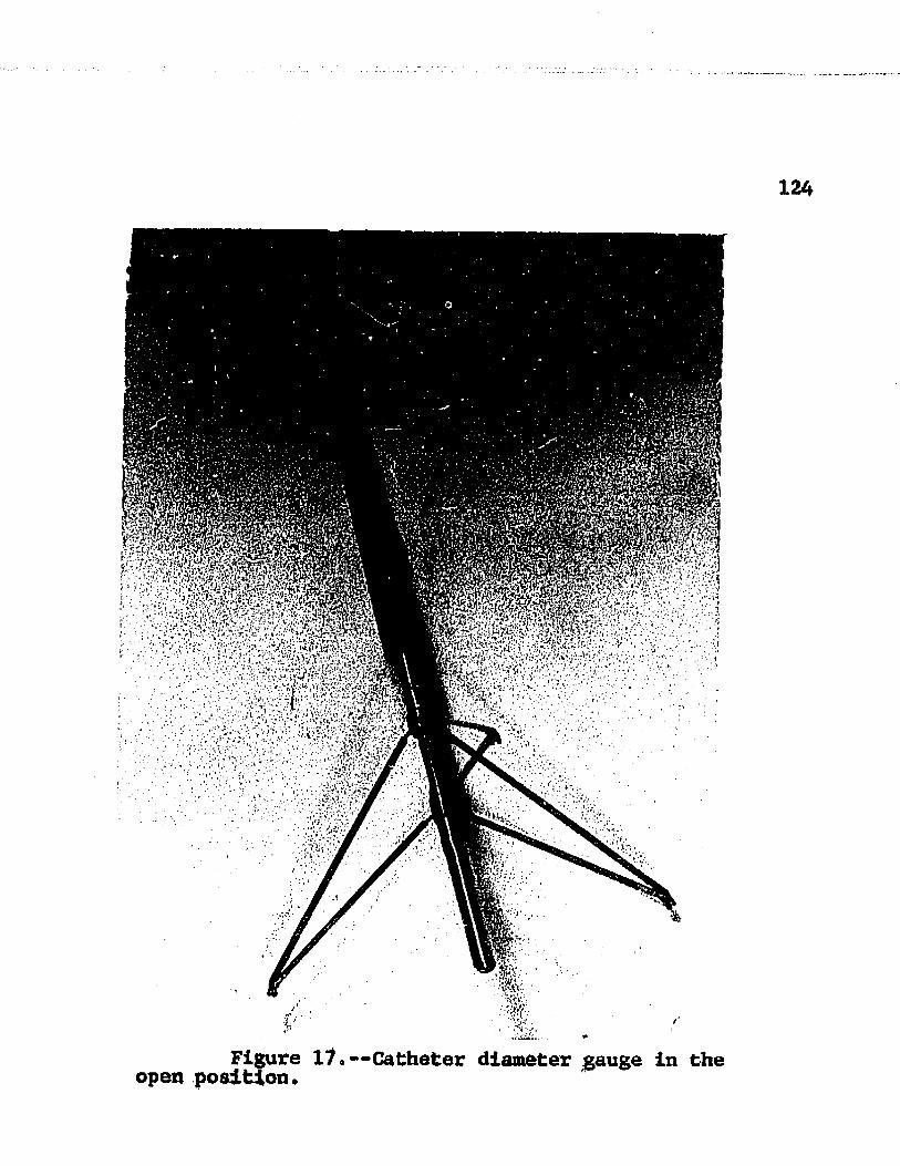
124

> * M K V t J f r f c A 1" » 1

Figure 17,--Catheter diameter gauge in the open position.

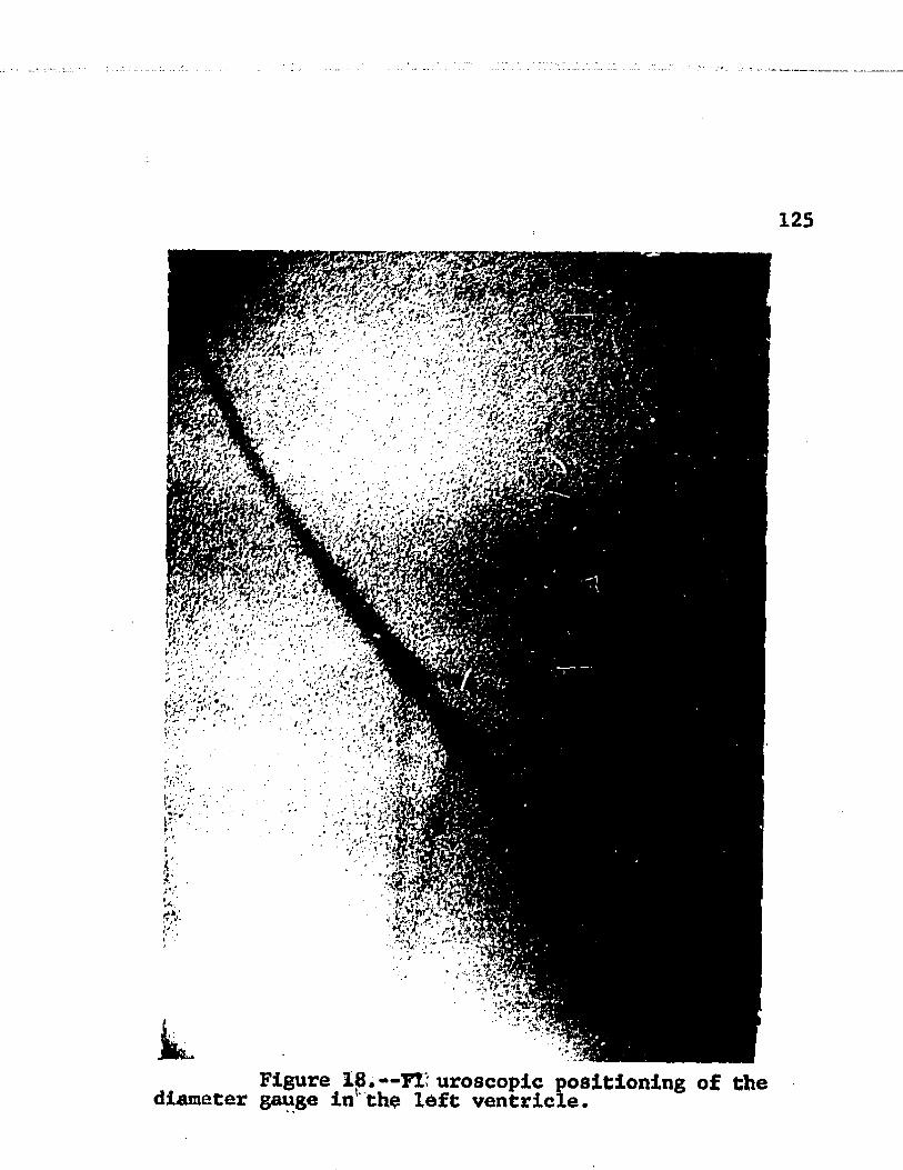
125

Figure 18.— FT uroscopic positioning of the diameter gauge in' the ldft ventricle.

126Both P(t) and D(t) data were monitored on a Sanborn oscilloscope prior to and during the recording.

The analog tape was digitized at 125 samples/see for use with an IBM 370/165 using OSU A/D convertor system.

tThis rate assures that no significant data is lost due to conversion, since the cardiac phenomena occurs at a low frequency (<£40 Hz).

The onset of diastole was defined at the minimum point of the D(t) waveform in a given cardiac cycle. The end of diastole was defined by noting the change in slope of the D(t) curve from the minimum point. Toward the end of diastole, the slope approaches zero. A computer program for automatic determination of both the onset and end of ventricular diastole, based on the above principle, is described in Appendix C. Due to the inherent problems associated with recording biological data, some noise spikes were present in the recorded data. Provision was included in the computer program (Appendix C) to suppress noise spikes, which were defined as abnormal changes in amplitude between successive sample points. P(t) diastolic points were chosen corresponding to the D(t) readings.

The data points thus obtained are then used in conjunction with the OMA developed in Chapter V to define a ventricular model in diastole (Chapter VII).

CHAPTER VII

SIMULATION EXPERIMENTS AND RESULTS

IntroductionThis chapter provides details of results obtained

from computer runs directed toward derivation of a valid mathematical representation of left ventricular behavior in diastole. As described earlier (Chapter II), this characterization is based on experimentally obtained left ventricular pressure, P(t), and left ventricular diameter, D(t), data. In the following a series of different differential equation forms are chosen starting with a linear first order form to fit the experimental data. A differential equation form yielding smallest possible sum squared error between model response and the observed output with the same input is identified as characterizing the left ventricular behavior (Chapter II). A number of cardiac cycle data are used for this derivation. Starting with the chosen form (above) attempts are then made to quantize the effects of various cardiac drugs on the diastolic phase.

General Comments on the Choice of Differential Equation Forms

It has already been described earlier that a valid analytic description of left ventricular diastolic behavior

127

is difficult to derive due to the arbitrary shape of the ventricle (Chapter II). Because of this difficulty, the diastolic behavior is better characterized from observed experimental data. Since there is no particular basis for choosing the differential equation forms with which the data are to be fitted, progressively higher order equations with linear and nonlinear terms have been utilized in this study.In this vein an initial attempt is made with a linear first order differential equation, relating the left ventricular diameter, D(t), and the rate of change of left ventricular diameter to the left ventricular pressure, P(t). Based on the above differential equation form computer runs are directed toward the derivation of an optimal set of coefficients with the stated objective of minimizing the sum squared error between the response from the said differential equation and the observed response. The first order equation, considered above, results in sum squared errors of greater than 40 (this corresponds to an error of 10% in fit), therefore, other terms such as ^jr2 have been added to the model equation resulting in progres­sively complex forms. Nonlinear differential equation forms have also been considered and their contributions in minimizing the sum squared error quantitated. While the number of differential equation forms that may be used is

129clearly arbitrary, it is felt that to be useful the parameters of the final proposed model should represent the physiologic event realistically. It has already been discussed (Chapter II) that the diastolic behavior is mainly a passive muscle phenomena. This constraint limits the choice of models (differential equations) to ones involving no active elements. In other words the coefficients of the differential equation should be constrained to be positive. Classically, muscle phenomena has been characterized in terms of viscous and elastic elements. This approach is deemed desirable in this study in view of the availability of various mechanical models describing the systolic behavior of the cardiac muscle so that a composite model for both phenomena may be derived. Therefore, the differential equation forms used in this chapter have been chosen with the constraints of defining passive muscle phenomena in terms of viscous and elastic elements. The particular elements of the differential equations may represent either linear or nonlinear properties. Even with this limitation, there are a large number of differential equations that can be studied. It is felt that the diastolic behavior characterization should at first be limited to differential equation forms which allow, at most, two distinct elastic and/or inertial elements. This limits the differential equation forms studied in this chapter

130to the second order forms. An attempt to characterize the left ventricular behavior using third order linear differential equation does not show any substantial reduction of sum squared error justifying the limitations imposed earlier.

Detailed Simulation Procedure used to Derive the Diastolic Model of Left Ventricular Behavior'

Experimental data from 10 animals have been used in this study (for details of experimental procedures see Chapter VI). Figure 19 describes a typical recording of the cardiac event. In the figure, LVP identifies the leftventricular pressure, P(t), and LVD the left ventriculardiameter, D(t). A total of 10 consecutive cycles from each animal have been utilized with the OMA developed in Chapter Vto derive a diastolic model of the left ventricular behavior.Table 8 depicts the diastolic measurements derived from a particular cardiac cycle of the recorded left ventricular pressure, F(t), and left ventricular diameter, D(t), waveforms. Based on earlier arguments, the observed pressure, P(t), is used with an assumed differential form to predict the response, D^(t).. The model response Dj (t) is then compared with D(t) and used with OMA (Chapter V) to derive the optimum parameters for the particular differential equation. In order to resolve the starting parameter vector bias, several

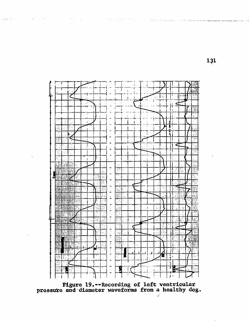
1?1

f

Figure 19*--Recording of left ventricular pressure and diameter waveforms from a healthy dog.

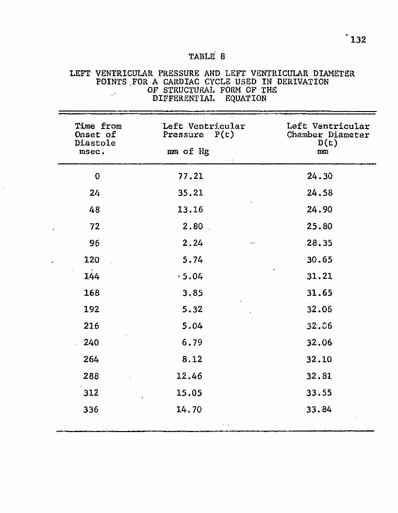
132TABLE 8

LEFT VENTRICULAR PRESSURE AND LEFT VENTRICULAR DIAMETER POINTS FOR A CARDIAC CYCLE USED IN DERIVATION

OF STRUCTURAL FORM OF THE DIFFERENTIAL EQUATION

Time from Onset of Diastole msec.

Left Ventricular Pressure P(t)mm of Hg

Left Ventricular Chamber Diameter D(t)

Tnrn

0 77.21 24.3024 35.21 24.5848 13.16 24.9072 2.80 . 25.8096 2.24 28.35

120 5.74 30.65144 -5.04 31.21168 3.85 31.65192 5.32 32.06216 5,04 32.06240 6.79 32.06264 8.12 32.10288 12.46 32.81312 15.05 33.55336 14.70 33.84

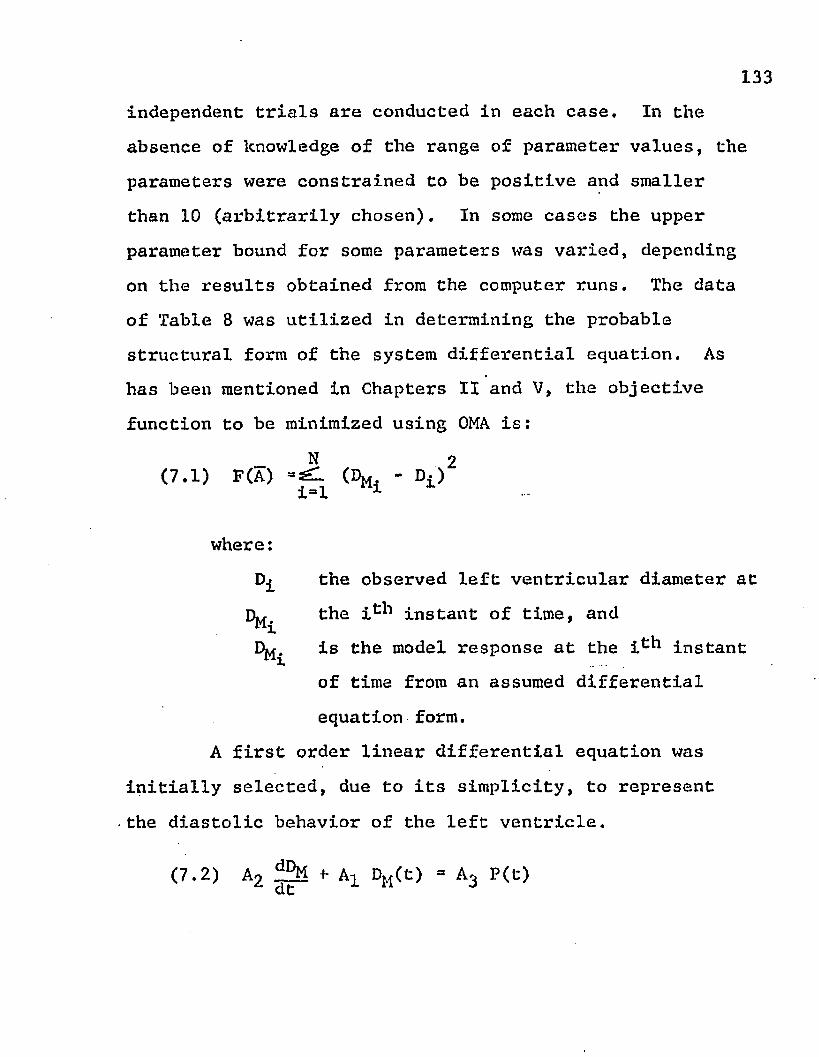
133independent trials are conducted in each case. In the absence of knowledge of the range of parameter values, the parameters were constrained to be positive and smaller than 10 (arbitrarily chosen). In some cases the upper parameter bound for some parameters was varied, depending on the results obtained from the computer runs. The data of Table 8 was utilized in determining the probable structural form of the system differential equation. As has been mentioned in Chapters II and V, the objective function to be minimized using OMA is:

N 2(7.1) F(A) -sC. (%, - Di) ial x

where:the observed left ventricular diameter at the i^ 1 instant of time, andis the model response at the i^ 1 instantof time from an assumed differential equation form.

A first order linear differential equation was initially selected, due to its simplicity, to represent the diastolic behavior of the left ventricle.

(7.2) A2 + Ax DM (t) = A3 P(t)

where:is the response of the model governed by equation 7.1.

P(t) is the observed pressure data (Table 8), and A- , Ag, and A3 are parameters which are determined from application of OMA to the above equation 7.2.

This equation as written above attempts to describe the left ventricular diastolic behavior in terms of a linear elastic element, A^/A^and a linear viscous element, A2/A3.All computations required in this chapter have been carried out in double-precision arithmetic correct up to sixteen decimal digits. For clarity of observation, however, the parameter values obtained from computer trials have been rounded off after four significant decimal digits. Table 9 describes the results of application of equation 7.2 with OMA to simulate the left ventricular behavior.

A total of 20 random searches were conducted in the entire parameter space (i.e., within the lower bound, 0 , and upper bound, 10, for all parameters) to locate the starting parameter vector, A°, (3.336, 1.7217, 0.3278) as shown in Trial 1 (Table 9). Because of earlier successes in reducing sum squared errors with known differential equation forms (Chapter V) LSMM was the only minimization method utilized with equation 7.2 initially. It was

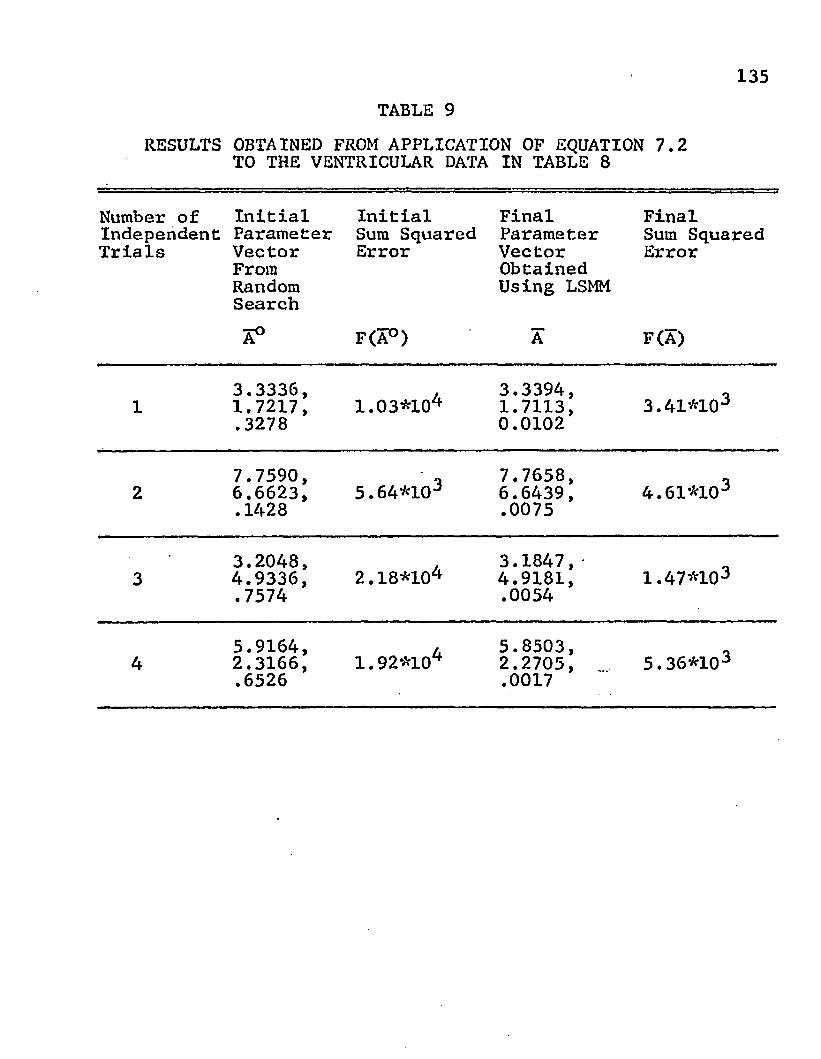
135TABLE 9

RESULTS OBTAINED FROM APPLICATION OF EQUATION 7.2TO THE VENTRICULAR DATA IN TABLE 8

Number ofIndependentTrials

InitialParameterVectorFromRandomSearch

Initial Sum Squared Error

Final Parameter Vector Obtained Using LSMM

FinalSum Squared Error

F(A°) A F(A)

13.3336,1.7217,.3278

1.03*1043.3394,1.7113,0.0102

3.41*103

27.7590,6.6623,.1428

5.64*1037.7658,6.6439,.0075

4.61*103

33.2048,4.9336,.7574

2.18*1043.1847,4.9181,.0054

1.47*103

45.9164,2.3166,.6526

1.92*104 5.8503,2.2705,.0017

5.36*103

136discovered using LSMM with the experimental data that the parameter change vectors generated were too large, resulting in violations of constraints. As can be seen in Table 9 (trials 1 to 4) the function reduction did take place but the final fit predicted by the equation was bad (sum squared error '^>1.47*10^). It was noticed that the gradient vectors at the end of each trial were large in magnitude, implying that a minima had not been reached. When the upper bound on two parameters were changed to 100, not much improvement in function value was observed. It was decided, therefore, to scale the deviation matrix {efy and the gradient vector, U, by the following (Marquardt®^):

a perceptible improvement in the magnitudes of the parameter change vector. This modification has been incorporated in the computer coding (Appendix A). Table 10 summarizes the final results obtained using equation 7.2.

above. Application of LSMM resulted in a further reduction of the model sum squared error to 47.53. The gradient

This normalization of the deviation matrix led to

A random search was carried out in the parameter space to locate the initial parameter vector A° as shown

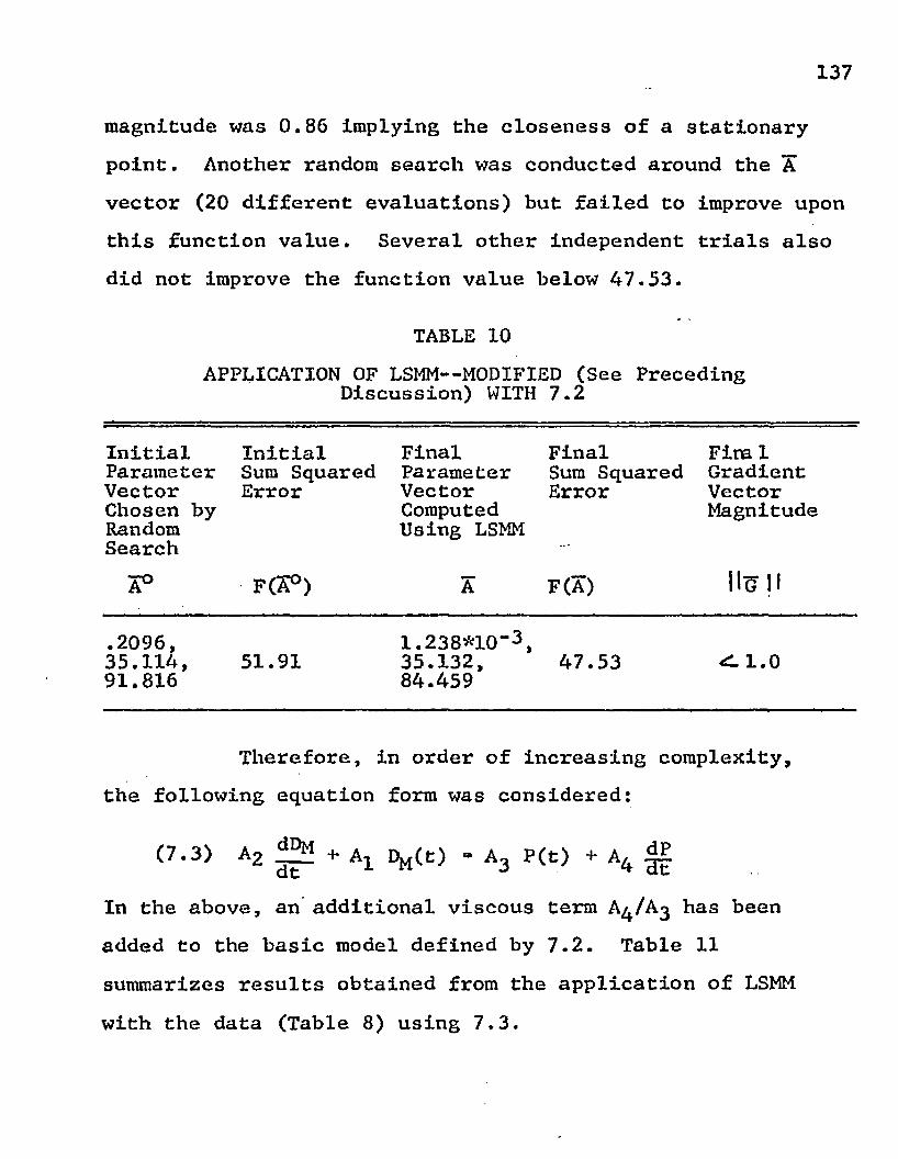
137

magnitude was 0.86 implying the closeness of a stationary point. Another random search was conducted around the A vector (20 different evaluations) but failed to improve upon this function value. Several other independent trials also did not improve the function value below 47.53.

TABLE 10APPLICATION OF LSMM--MODIFIED (See Preceding

Discussion) WITH 7.2

Initial Initial Final Final Fira 1Parameter Sum Squared Parameter Sum Squared GradientVector Error Vector Error VectorChosen by Computed MagnitudeRandom Using LSMMSearchA° F(A°) A F(A) iis 11

.2096, 1.238*10~3 ,35.114, 51.91 35.132, 47.53 «£-1.091.816 84.459

Therefore, in order of increasing complexity, the following equation form was considered:

(7.3) A2 + Ax D^t) - A3 P(t) + A4In the above, an additional viscous term A4/A3 has been added to the basic model defined by 7.2. Table 11 summarizes results obtained from the application of LSMM with the data (Table 8) using 7.3.

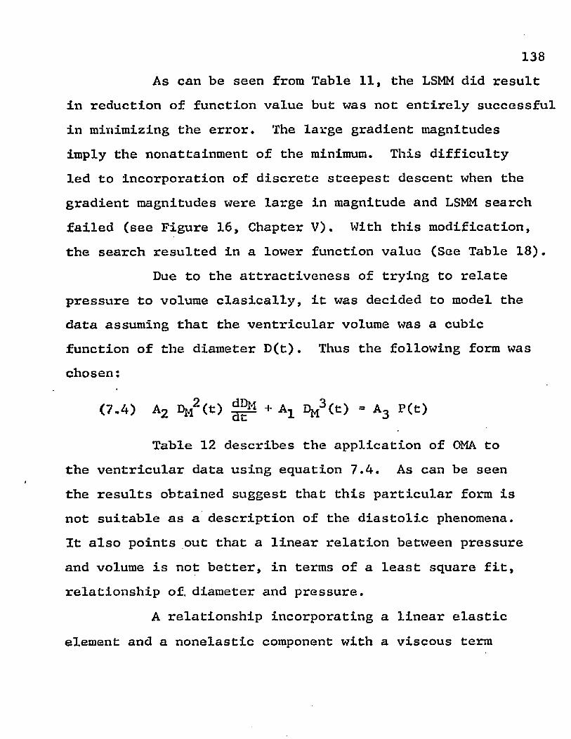
138As can be seen from Table 11, the LSMM did result

in reduction of function value but was not entirely successful in minimizing the error. The large gradient magnitudes imply the nonattainment of the minimum. This difficulty led to incorporation of discrete steepest descent when the gradient magnitudes were large in magnitude and LSMM search failed (see Figure 16, Chapter V). With this modification, the search resulted in a lower function value (See Table 18).

Due to the attractiveness of trying to relate pressure to volume clasically, it was decided to model the data assuming that the ventricular volume was a cubic function of the diameter D(t). Thus the following form was chosen:

(7.4) A2 DM2 (t) + Ax ^ ( t ) = A3 P(t)

Table 12 describes the application of OMA to the ventricular data using equation 7.4. As can be seen the results obtained suggest that this particular form is not suitable as a description of the diastolic phenomena.It also points out that a linear relation between pressure and volume is not better, in terms of a least square fit, relationship of. diameter and pressure.

A relationship incorporating a linear elastic element and a nonelastic component with a viscous term

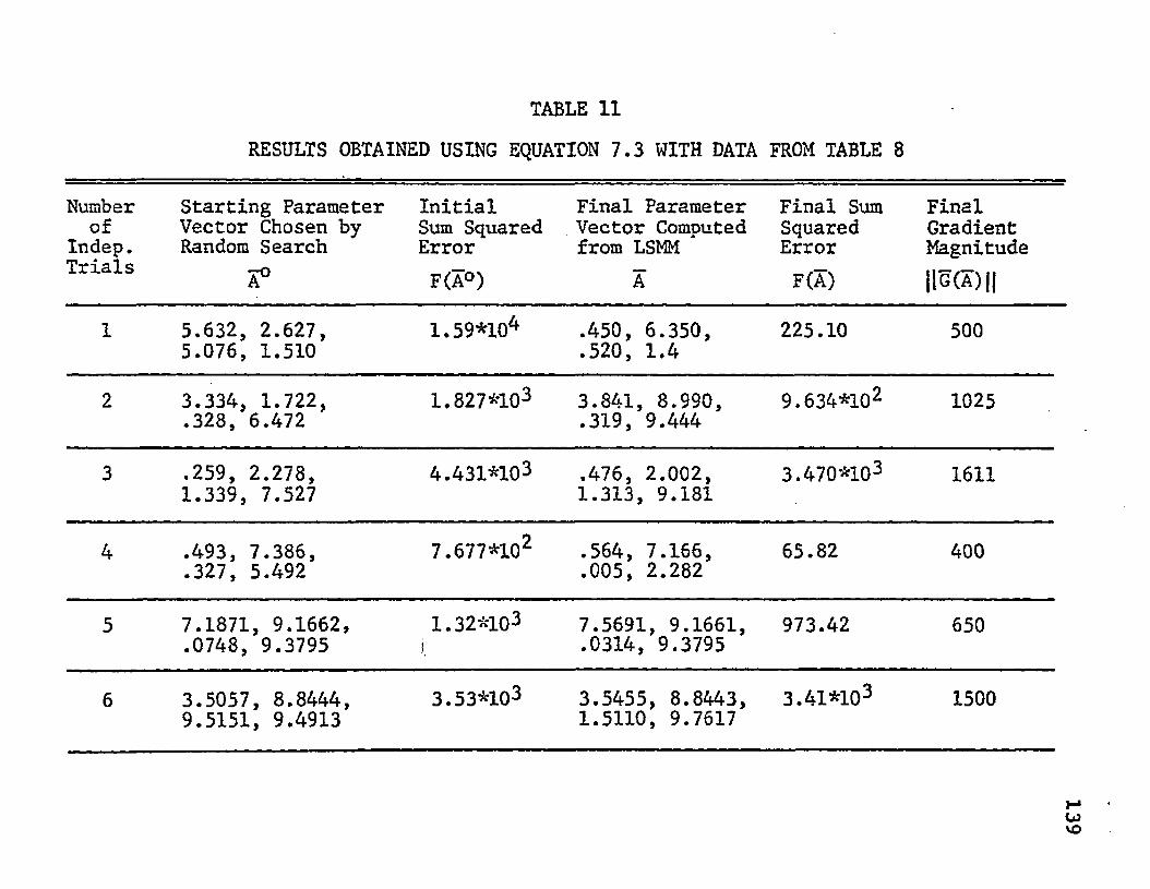
TABLE 11RESULTS OBTAINED USING EQUATION 7.3 WITH DATA FROM TABLE 8

Numberof

Indep.Trials

Starting Parameter Vector Chosen by Random Search

A°

Initial Sum Squared ErrorF(A°)

Final Parameter Vector Computed from LSMM

A

Final SumSquaredErrorF(A)

FinalGradientMagnitude||g (A) ||

1 5.632, 2.627, 5.076, 1.510

1.59*104 .450, 6.350, .520, 1.4

225.10 500

2 3.334, 1.722, .328, 6.472

1.827*103 3.841, 8.990, .319, 9.444

9.634*10^ 1025

3 .259, 2.278, 1.339, 7.527

4.431*103 .476, 2.002, 1.313, 9.181

3.470*103 1611

4 .493, 7.386, .327, 5.492

7.677*102 .564, 7.166, .005, 2.282

65.82 400

5 7.1871, 9.1662, .0748, 9.3795

1.32*103 7.5691, 9.1661, .0314, 9.3795

973.42 650

6 3.5057, 8.8444, 9.5151, 9.4913

3.53*103 3.5455, 8.8443, 1.5110, 9.7617

3.41*103 1500

139

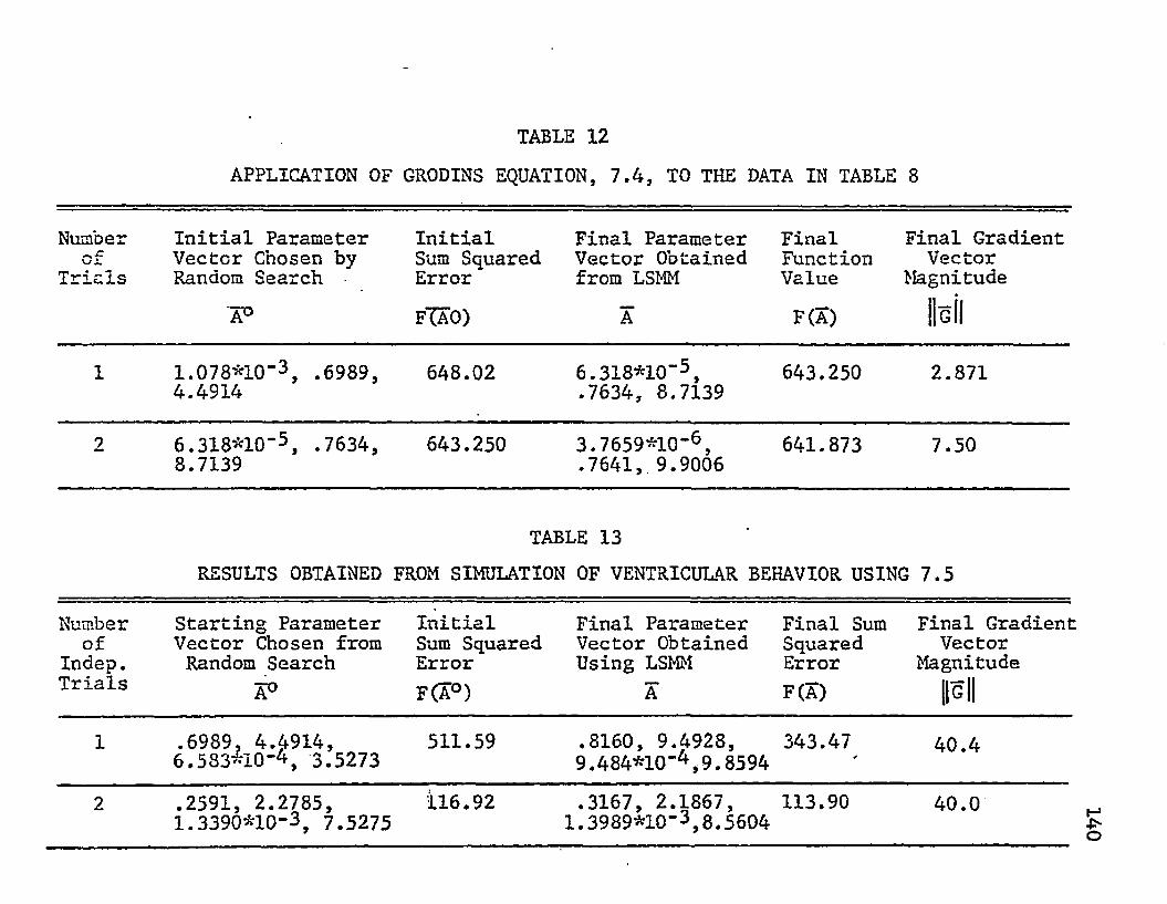
TABLE 12APPLICATION OF GRODINS EQUATION, 7.4, TO THE DATA IN TABLE 8

Numberof

TrialsInitial Parameter Vector Chosen by Random Search

Initial Sum Squared Error

Final Parameter Vector Obtained from LSMM

FinalFunctionValue

Final Gradient Vector

MagnitudeA° fTa o ) A F(A) IIg II

1 1.078*10”3, .6989, 4.4914

648.02 6.318*10"5, .7634, 8.7139

643.250 2.871

2 6.318*10"5, .7634, 8.7139

643.250 3.7659*10“6, .7641, 9.9006

641.873 7.50

TABLE 13RESULTS OBTAINED FROM SIMULATION OF VENTRICULAR BEHAVIOR USING 7.5

Numberof

Indep.Trials

Starting Parameter Vector Chosen from Random Search

A°

Initial Sum Squared ErrorF(A°)

Final Parameter Vector Obtained Using LSMM

A

Final SumSquaredErrorF(A)

Final Gradient Vector

MagnitudeIlGlI

1 .6989, 4.4914, 6.583*10-4, 3.5273 511.59 .8160, 9.4928, 9.484*10“4,9.8594

343.47 40.4

2 .2591, 2.2785, 1.3390*10-3, 7.5275116.92 .3167, 2.1867,

1.3989*10-3,8.5604113.90 40.0 140

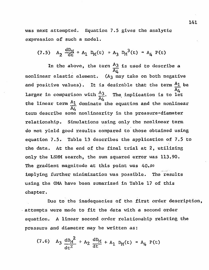
141was next attempted. Equation 7.5 gives the analytic expression of such a model.

(7.5) A2 + Ax D^t) + A3 % 3(t) - A4 P(t)

In the above, the tern ^3 is used to describe a^4

nonlinear elastic element. (A3 may take on both negativeand positive values). It is desirable that the term ^1 be

Alarger in comparison with The implication is to letA4the linear term ^1 dominate the equation and the nonlinear

A4terra describe some nonlinearity in the pressure-diameter relationship. Simulations using only the nonlinear terra do not yield good results compared to those obtained using equation 7.5. Table 13 describes the application of 7.5 to the data. At the end of the final trial at 2, utilizing only the LSMM search, the sum squared error was 113.90.The gradient magnitude at this point was 40.0o implying further minimization was possible. The results using the OMA have been sumarized in Table 17 of this chapter.

Due to the inadequacies of the first order description, attempts were made to fit the data with a second order equation. A linear second order relationship relating the pressure and diameter may be written as:

2(7.6) A3 dDM -1- A2 ^ + Ax DM (t) - A4 P(t)

dt2 dt

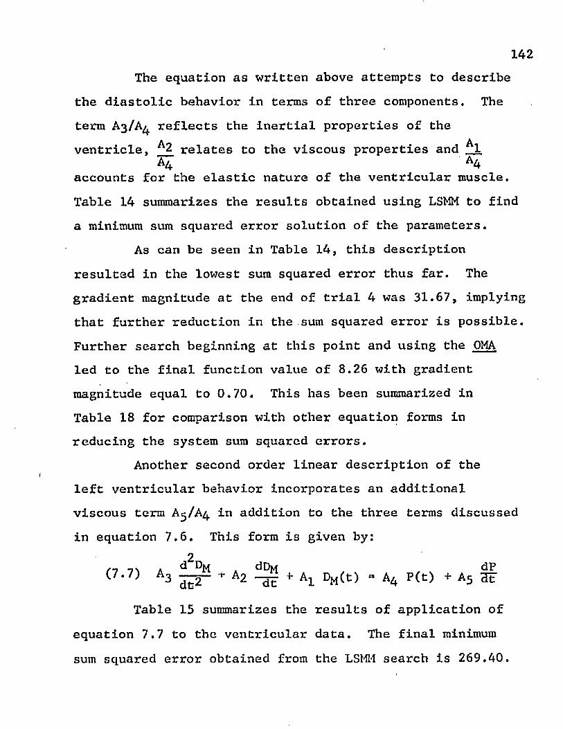
142The equation as written above attempts to describe

the diastolic behavior in terms of three components. Theterm A3/A4 reflects the inertial properties of theventricle, ^2 relates to the viscous properties and ^1

A4 a4accounts for the elastic nature of the ventricular muscle.Table 14 summarizes the results obtained using LSMM to finda minimum sum squared error solution of the parameters.

As can be seen in Table 14, this description resulted in the lowest sum squared error thus far. The gradient magnitude at the end of trial 4 was 31.67, implying that further reduction in the sum squared error is possible. Further search beginning at this point and using the OMA led to the final function value of 8.26 with gradient magnitude equal to 0.70. This has been summarized in Table 18 for comparison with other equation forms in reducing the system sum squared errors.

Another second order linear description of the left ventricular behavior incorporates an additional viscous term A5/A4 in addition to the three terms discussed in equation 7.6. This form is given by:

2. d dDM dP(7.7) A3 _ _ + A2 -^2 + Al DM (t) - A4 P(t) + A5 3t

Table 15 summarizes the results of application of equation 7.7 to the ventricular data. The final minimum sum squared error obtained from the LSMM search is 269.40.

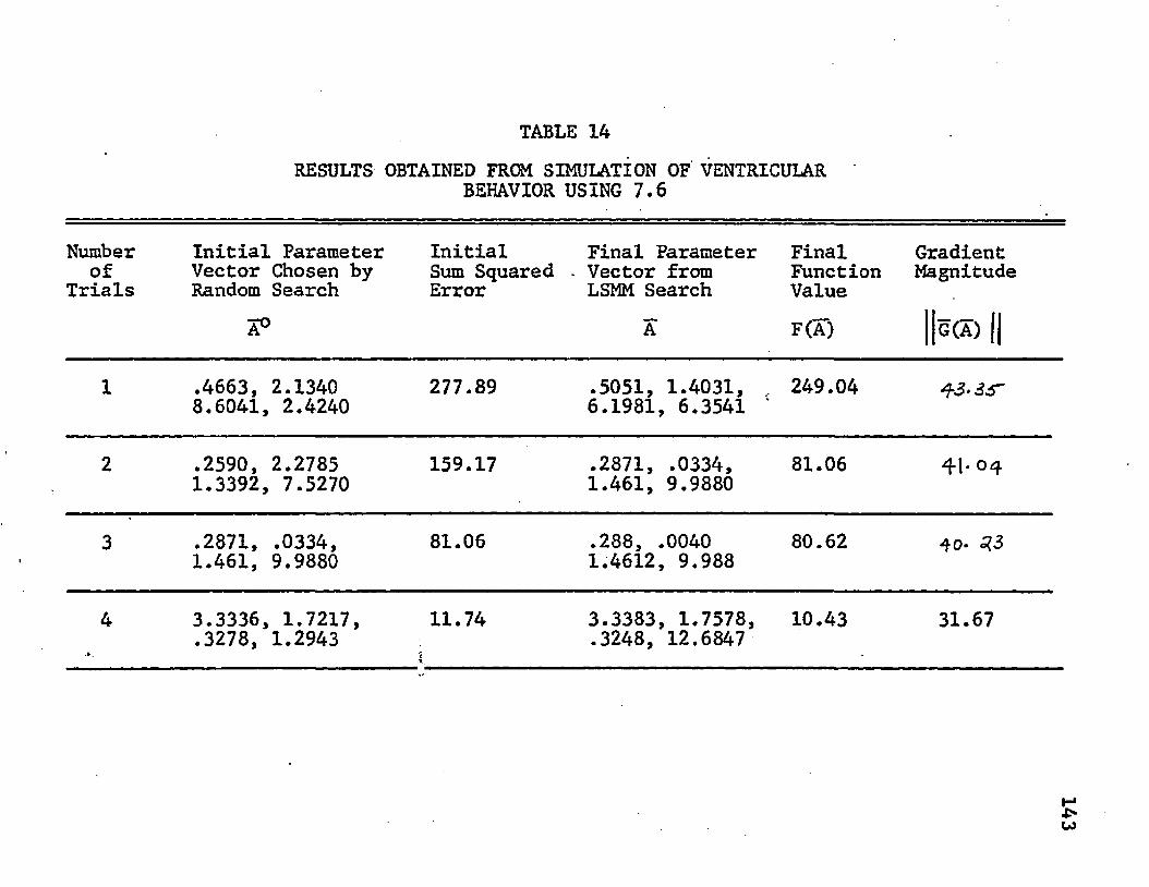
TABLE 14RESULTS OBTAINED FROM SIMULATION OF VENTRICULAR

BEHAVIOR USING 7.6

Numberof

TrialsInitial Parameter Vector Chosen by Random Search

A°

Initial Sum Squared Error

Final Parameter - Vector from LSMM Search

A

FinalFunctionValueF(A)

GradientMagnitude

||g (a ) ||

1 .4663, 2.1340 8.6041, 2.4240

277.89 .5051, 1.4031, . 6.1981, 6.3541 *

249.04 4-3-33-

2 .2590, 2.2785 1.3392, 7.5270

159.17 .2871, .0334, 1.461, 9.9880

81.06 4r\' °4

3 .2871, .0334, 1.461, 9.9880

81.06 .288, .0040 1.4612, 9.988

80.62 40* 33

4 3.3336, 1.7217, 11.74 3.3383, 1.7578, 10.43 31.67.3278, 1.2943

ii V

.3248, 12.6847

143

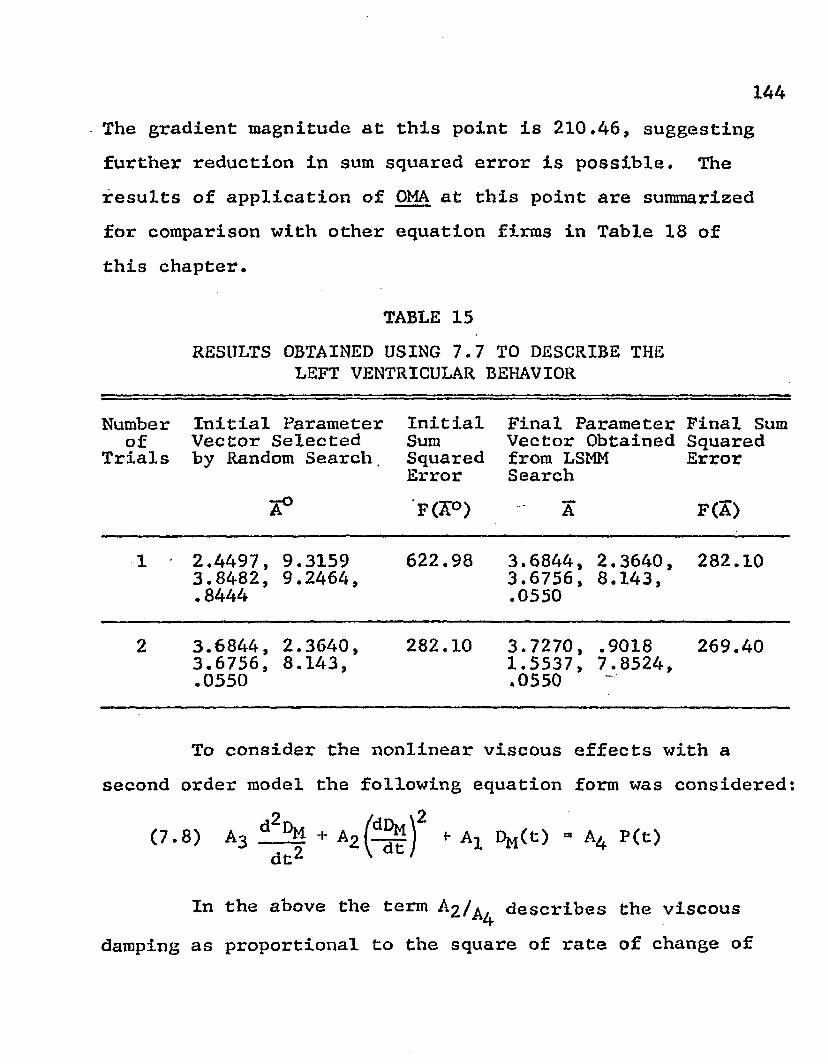
144The gradient magnitude at this point is 210.46, suggesting further reduction in sum squared error is possible. The results of application of OMA at this point are summarized for comparison with other equation firms in Table 18 of this chapter.

TABLE 15RESULTS OBTAINED USING 7.7 TO DESCRIBE THE

LEFT VENTRICULAR BEHAVIOR

NumberofTrials

Initial Parameter Vector Selected by Random Search.

InitialSumSquaredError

Final Parameter Vector Obtained from LSMM Search

Final SumSquaredError

F(X°) ■ ■■A F(A>

1 2.4497, 9.3159 3.8482, 9.2464, . 8444

622.98 3.6844,3.6756,.0550

2.3640,8.143,

282.10

2 3.6844, 2.3640, 3.6756, 8.143, .0550

282.10 3.7270,1.5537,.0550

.90187.8524,

269.40

To consider the nonlinear viscous effects with asecond order model the following equation form was considered:

2 / «2(7.8) A3 d foj + <• Ax DfjCt) =■ A4 P(t)

In the above the term describes the viscousdamping as proportional to the square of rate of change of

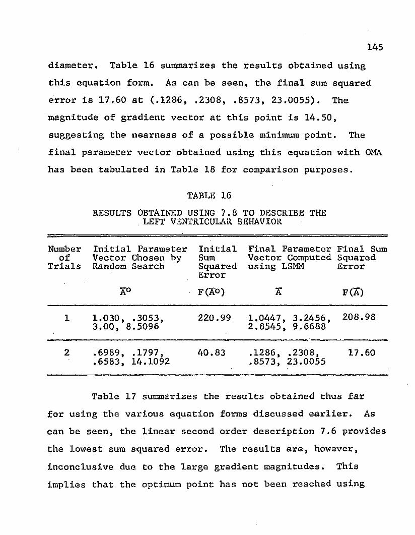
145diameter. Table 16 summarizes the results obtained using this equation form. As can be seen, the final sura squared error is 17.60 at (.1286, .2308, .8573, 23.0055). The magnitude of gradient vector at this point is 14.50, suggesting the nearness of a possible minimum point. The final parameter vector obtained using this equation with OMA has been tabulated in Table 18 for comparison purposes.

TABLE 16RESULTS OBTAINED USING 7.8 TO DESCRIBE THE

LEFT VENTRICULAR BEHAVIOR

Numberof

TrialsInitial Parameter Vector Chosen by Random Search

InitialSumSquaredError

Final Parameter Final Sum Vector Computed Squared using LSMM Error

X° F(Xo) X F(A)

1 1.030, .3053, 3.00, 8.5096 220.99 1.0447, 3.2456,

2.8545, 9.6688208.98

2 .6989, .1797, .6583, 14.1092

40.83 .1286, .2308, .8573, 23.0055

17.60

Table 17 summarizes the results obtained thus far for using the various equation forms discussed earlier. As can be seen, the linear second order description 7.6 provides the lowest sum squared error. The results are, however, inconclusive due to the large gradient magnitudes. This implies that the optimum point has not been reached using

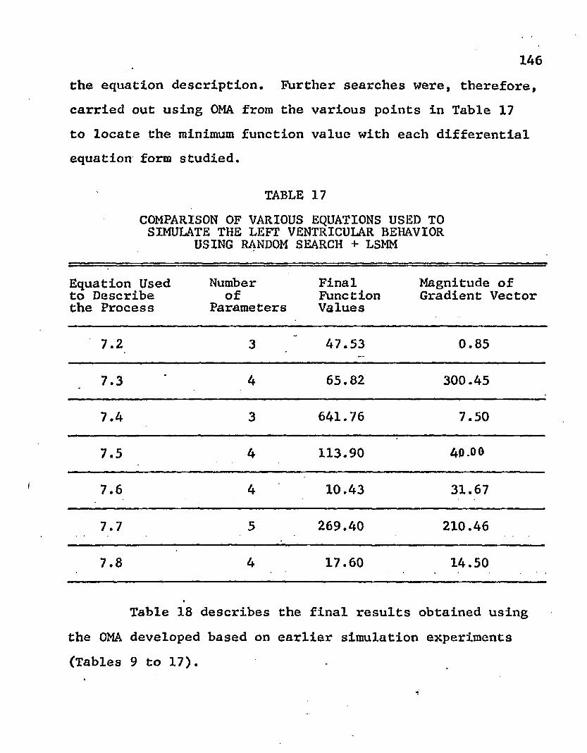
146

Che equation description. Further searches were, therefore, carried out using OMA from the various points in Table 17 to locate the minimum function value with each differential equation form studied.

TABLE 17COMPARISON OF VARIOUS EQUATIONS USED TO SIMULATE THE LEFT VENTRICULAR BEHAVIOR

USING RANDOM SEARCH + LSMM

Equation Used to Describe the Process

NumberofParameters

FinalFunctionValues

Magnitude of Gradient Vector

7.2 3 47.53 0.85

7.3 4 65.82 300.45

7.4 3 641.76 7.50

7.5 4 113.90 40-00

7.6 4 10.43 31.67

7.7 5 269.40 210.46

7.8 4 17.60 14.50

Table 18 describes the final results obtained using the OMA developed based on earlier simulation experiments (Tables 9 to 17).

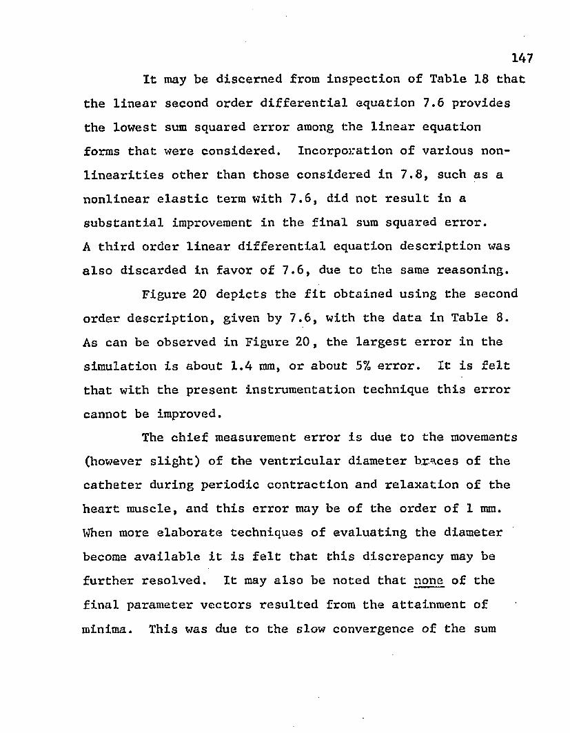
147It may be discerned from inspection of Table 18 that

the linear second order differential equation 7.6 provides the lowest sum squared error among the linear equation forms that were considered. Incorporation of various non- linearities other than those considered in 7.8, such as a nonlinear elastic term with 7.6, did not result in a substantial improvement in the final sum squared error.A third order linear differential equation description was also discarded in favor of 7.6, due to the same reasoning.

Figure 20 depicts the fit obtained using the second order description, given by 7.6, with the data in Table 8.As can be observed in Figure 20, the largest error in the simulation is about 1.4 ram, or about 5% error. It is felt that with the present instrumentation technique this error cannot be improved.

The chief measurement error is due to the movements (however slight) of the ventricular diameter braces of the catheter during periodic contraction and relaxation of the heart muscle, and this error may be of the order of 1 mm.When more elaborate techniques of evaluating the diameter become available it is felt that this discrepancy may be further resolved. It may also be noted that none of the final parameter vectors resulted from the attainment of minima. This was due to the slow convergence of the sum

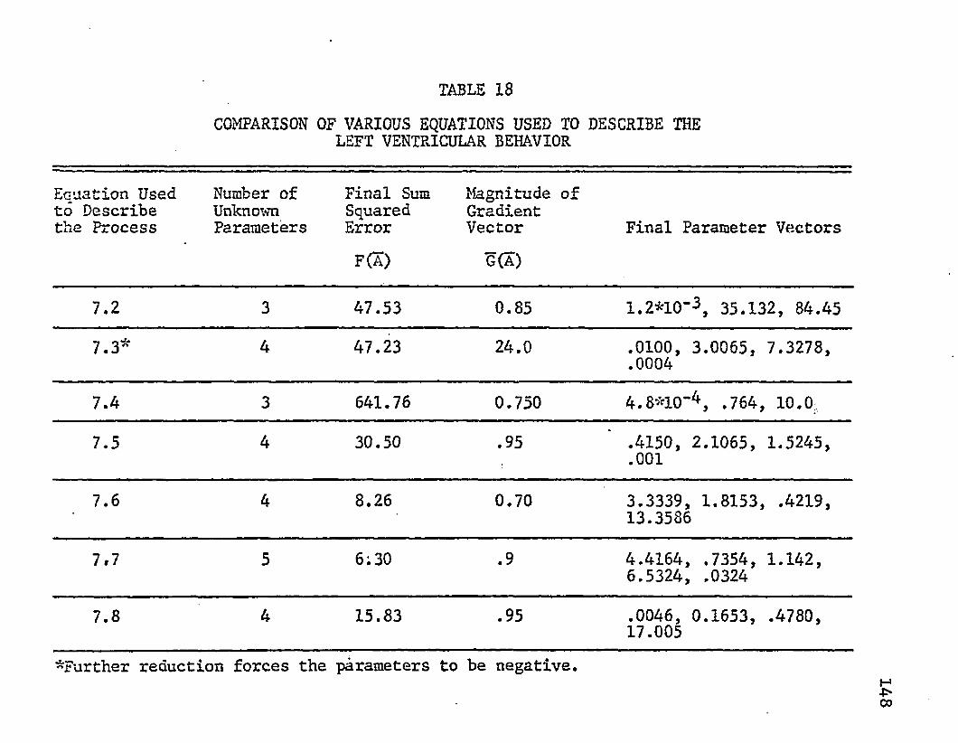
TABLE 18COMPARISON OF VARIOUS EQUATIONS USED TO DESCRIBE THE

LEFT VENTRICULAR BEHAVIOR

Equation Used to Describe the Process

Number ofUnknownParameters

Final SumSquaredErrorF(A)

Magnitude ofGradientVector

G(A)Final Parameter Vectors

7.2 3 47.53 0.85 1.2*10"3, 35.132, 84.45

7.3* 4 47.23 24.0 .0100, 3.0065, 7.3278, .0004

7.4 3 641.76 0.750 4.8*10"4, .764, 10.0,

7.5 4 30.50 .95 .4150, 2.1065, 1.5245, .001

7.6 4 8.26 0.70 3.3339, 1.8153, .4219, 13.3586

7*7 5 6; 30 .9 4.4164, .7354, 1.142, 6.5324, .0324

7.8 4 15.83 .95 .0046, 0.1653, .4780, 17.005

^Further reduction forces the parameters to be negative. 148

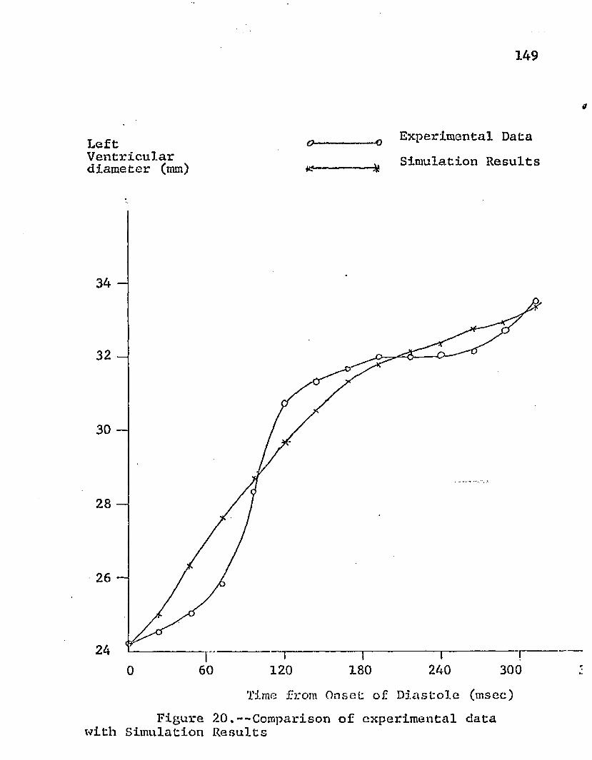
149

0________0 Experimental DataVentricular Simulation Resultsdiameter (mm) «------- M

30

28

240 300120 180600Time from Onset of Diastole (msec)

Figure 20 *--Comparison of experimental data with Simulation Results

150squared error of less than 10 percent. If this criteria is removed from the program further improvement may take place, however, in a feasibility study undertaken here this refinement of minima may not be worthwhile. This has been observed in case of the second order differential equation where further lowering of function values took a large number of functional evaluations (/'130) to result in a final function value of 8.24. Gradient at this point is given by .25. This compares with 8.26 obtained with gradient of .7.

Comparison of Variations in Parameters using Equation T.6 to Describe the Left Ventricular Behavior for an Animal

Equation 7.6 was next used with data from ten consecutive cycles in which the period of diastole was relatively constant. The end systolic pressure in this . period measured 77.21 £ 10 mm of Hg and the end systolic" diameter was 24.296 2 mm. The end diastolic pressurewas 14.70 3 mm. of Hg and the end diastolic diametervaried between 31.842 and 35.00 mm. The final sura squared error using the second order equation was found to be less than 10.0. In-spite of changes in the observed pressure and diameter waveforms the changes in final parameter values were less than 5 percent, suggesting that the coefficients may describe the ventricular properties.

Effects of Period of DiastoleTable 19 shows the diastolic data when the period of

diastole was lower than that in Table 8. The parameter values obtained in this case are given by (7.095, .7605,.9701, 16.1142) and the final sum squared error is 14.31.As may be discerned, the data is fitted very closely by the second order model. When the period of diastole was 264 msec, only the parameter vector is given by (1.4385, .5881, .3278, 14.0189). All the above data refers to measurements taken from one dog. As can be discerned, the parameter vectors, representing muscle properties, show a great dependence on the period of diastole. When the second order differential equation was fitted with data from other dogs used in the study, the fluctuations in the coefficient values were much wider. However, a comparison of the coefficient values is not realistic in view of the decided dependence of the model on the period of diastole. Continuing efforts will characterize the differences in parameters t-rtien the heart rate is maintained constant by atrial pacing.

Variations in Parameter Values With Quinidine and Isopreternol

An attempt was made to describe the effects on muscle properties of two potent cardiac drugs, Quinidine and Isopreternol. Figure 21 shows the effects of administration of Quinidine. Quinidine is a negative inotrope and results

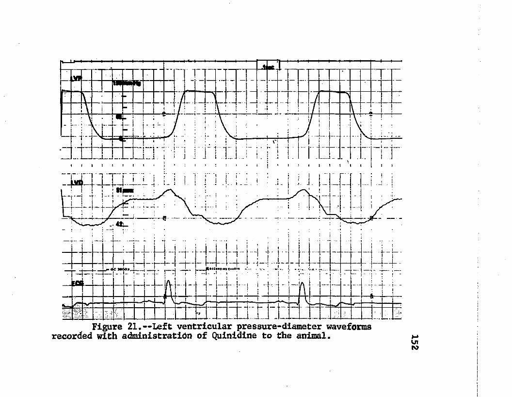
Figure 21.--Left ventricular pressure-diameter waveformsrecorded with administration of Quinidine to the animal. mUi

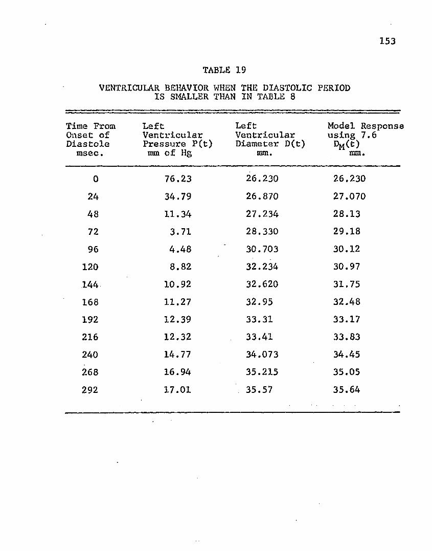
153

TABLE 19VENTRICULAR BEHAVIOR WHEN THE DIASTOLIC PERIOD

IS SMALLER THAN IN TABLE 8

Time From Onset of Diastole msec.

LeftVentricular Pressure P(t) mm of Hg

LeftVentricular Diameter D(t) mm.

Model Response using 7.6 %(t) mm.

0 76.23 26.230 26.23024 34.79 26.870 27.07048 11.34 27.234 28.1372 3.71 28.330 29.1896 4.48 30.703 30.12

120 8.82 32.234 30.97144 10.92 32.620 31.75168 11.27 32.95 32.48192 12.39 33.31 33.17216 12.32 33.41 33.83240 14.77 34.073 34.45268 16.94 35.215 35.05292 17.01 35.57 35.64

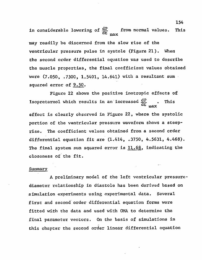
154in considerable lowering of 4Z from normal values. This

dt maxmay readily be discerned from the slow rise of theventricular pressure pulse in systole (Figure 21). Whenthe second order differential equation was used to describethe muscle properties, the final coefficient values obtainedwere (7.050, .7300, 1.5401, 14.641) with a resultant sumsquared error of 9.50.

Figure 22 shows the positive inotropic effects ofIsopreternol which results in an Increased SjZ . This

maxeffect is clearly observed in Figure 22, where the systolic portion of the ventricular pressure waveform shows a steep- rise. The coefficient values obtained from a second order differential equation fit are (1.414, .3750, 4.5631, 4.468). The final system sum squared error is 11.68, indicating the closeness of the fit.

SummaryA preliminary model of the left ventricular pressure

diameter relationship in diastole has been derived based on simulation experiments using experimental data. Several first and second order differential equation forms were fitted with the data and used with OMA to determine the final parameter vectors. On the basis of simulations in this chapter the second order linear differential equation

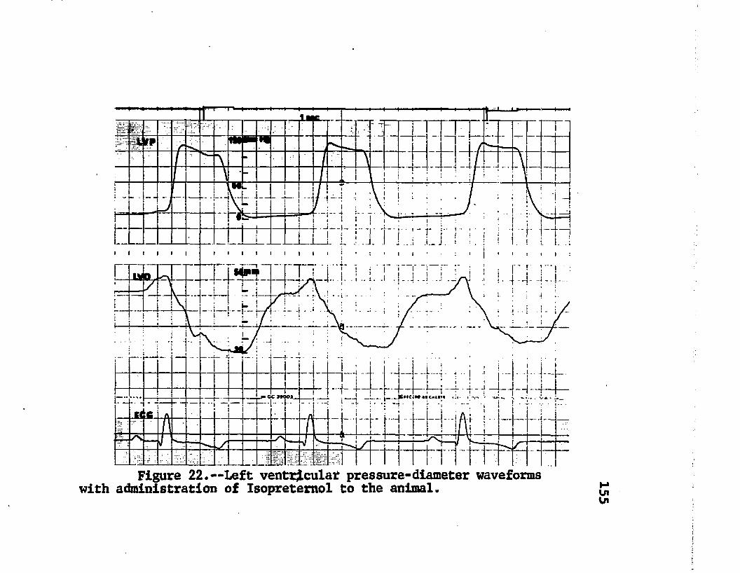
Figure 22.--Left ventricular pressure-diameter waveforms with administration of Isopreternol to the animal. 155

has been observed to fit the data best. The error in simulations using the second order differential equation is less than 5 percent. It has been observed that the inadequacies of present measurement techniques lead.to the same magnitude of errors in the experimental data and, therefore, further simulations to try to reduce this simulation error have been ruled out. The decided dependence of the parameters of the differential equation on the period of diastole obscures the comparison of the muscle properties of various animals used in the study. It has been shown that Qui.nidine and Isopreternol reflect in changes of the diastolic pressure-diameter relationship.

CHAPTER VIII

DISCUSSION

In troductionThis chapter begins with a critical reviex* of the

experimental results obtained using the OMA developed In this dissertation. The limitations and the advantages of the approach used in the study are compared. The salient features of the ventricular model derived are discussed and its scope and usefulness are also described. The work of other'investigators in contrast to the OMA developed here are discussed and compared.

Limitation of the Experimental Technique

The model developed in this study has been derived based on minimization of sum squared error between the predicted response and the observed response. This computation was performed at every 8 msec. Interval. It is felt that a better fit may be obtained by attempting to compute the sum squared error at every one msec. This will lead to a better description of the objective function used with the OMA. However, this was not attempted in this

157

dissertation in view of the measurement errors that have been previously discussed (Chapter VII).

In addition, due to the mechanical nature of the diameter gauge, errors are present in the recorded diameter. The calibration of the diameter gauge is also in considerable error. This calibration is at present accomplished by drawing the gauge through a series of concentric rings of various known diameters. Since the process is done by hand, considerable margin for error exists. Calibration of the pressure manometer is done in vitro using a mercury manometer and, therefore, there is a possibility of errors resulting from this procedure as well. Also the catheter tip manometer may collect fibrin deposits in vivo which may interfere with the output.

The foregoing limitations induced by the present level of sophistication of measurement techniques allow for a degree of measurement errors that defies improvement at this time. Until these measurement techniques have been improved, nothing may be gained by reducing the simulation and computational errors.

Scope and Usefulness of the Present Ventricular 'Mocfel

A new mathematical description of ventricular filling (i.e.., compliance) has been developed In this study. It has

been shown from simulation experiments in Chapter VII that this description is very dependent upon the period of diastole. This conforms with the classical physiological concepts of cardiac dynamics as expressed by Frank and Starling. The earlier hypothesis (Chapter I) that the coefficients of the equation describe muscle properties has been justified from the results of this study. This is so (true) because several cycles of ventricular data (when the period was relatively constant) resulted in essentially no change in parameter values with variations in both pressure and diameter waveforms. In the absence of a valid theoretical framework defining pressure-diameter relationship, it is difficult to prove the uniqueness of the present model.However, based on Zadeh*s definition (Chapter II) the model developed in this study is optimum and equivalent to all others that may be derived using the same criteria.

It is known that dogs naturally have respiratory induced sinus arrythmia. Thus, the period of diastole varies with respiration. Therefore, if this model is to be used for further studies in the dog, the heart rate must be maintained constant by artrial pacing. This is because it has already been mentioned that the model shows strong dependence on the period of diastole. An interesting test for the model would be to study compliance in animals with

160

left ventricular hypertrophy and/or dilatalis. In these conditions the muscle fibers have histogically obvious changes in their dimensions (Hamlin personal communication).

The model developed in this study is based on the intraventricular pressure and not the transmutal distending pressure. In order to derive a more realistic model, it is felt that continuing experiments be performed in open-chest animals or means to monitor intrapleural pressure be devised in case of closed-chest animals. Nonetheless, based on personal observations, I feel that intrapleural pressure could be neglected or at least taken as a constant in a feasibility study attempted here.

Left ventricular pressure and left ventricular diameter measurements were also obtained from other laboratories (Dr. Pieper, Dr. Hawthorne). The second order differential equation form provided the lowest sum-squared error in these cases as well. This justifies, notwithstanding the current measurement inaccuracies, the validity of the approach.

As has already been mentioned in Chapter I, the potential usefulness of this study is in characterization of ventricular compliance in various diseased states. This is because adequate therapy can only be instituted when one has defined distensibility. For example, if the left

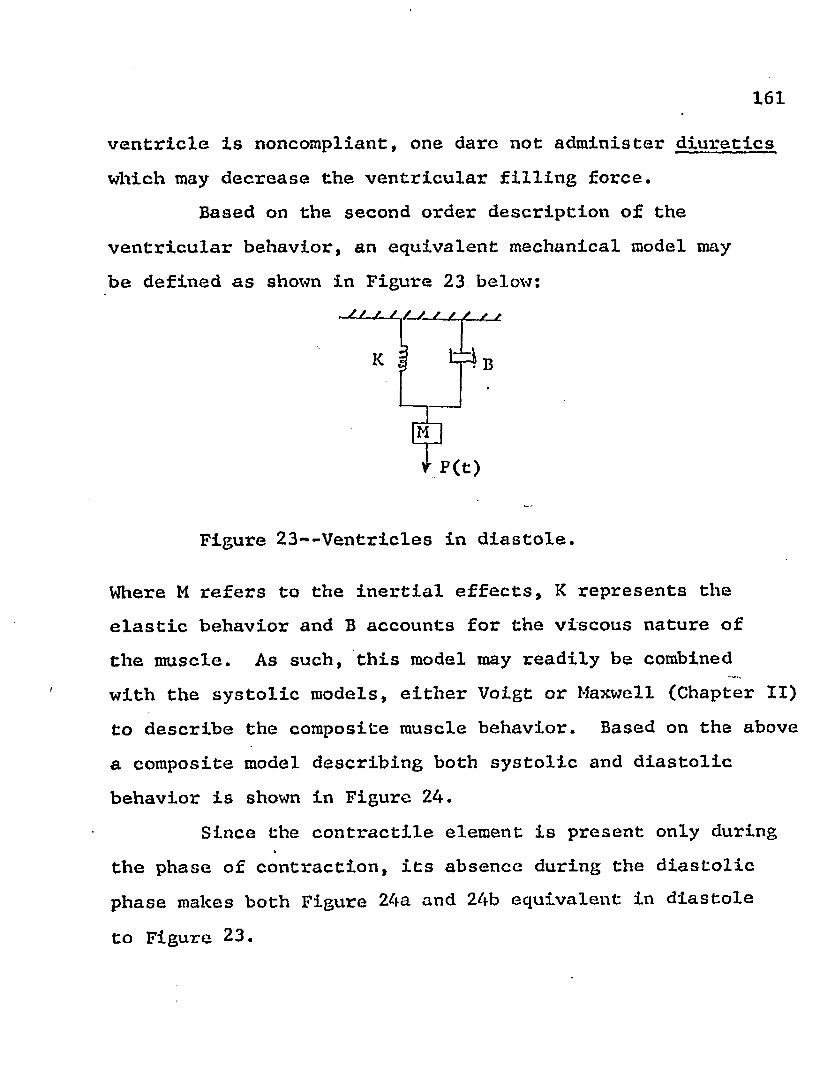
161

ventricle is noncompliant, one dare not administer diuretics which may decrease the ventricular filling force.

ventricular behavior, an equivalent mechanical model may be defined as shown in Figure 23 below:

Where M refers to the inertial effects, K represents the elastic behavior and B accounts for the viscous nature of the muscle. As such, this model may readily be combined with the systolic models, either Voigt or Maxwell (Chapter II) to describe the composite muscle behavior. Based on the above a composite model describing both systolic and diastolic behavior Is shown in Figure 24.

the phase of contraction, its absence during the diastolic phase makes both Figure 24a and 24b equivalent in diastole to Figure 23.

Based on the second order description of the

Figure 23--Ventricles In diastole.

Since the contractile element is present only during

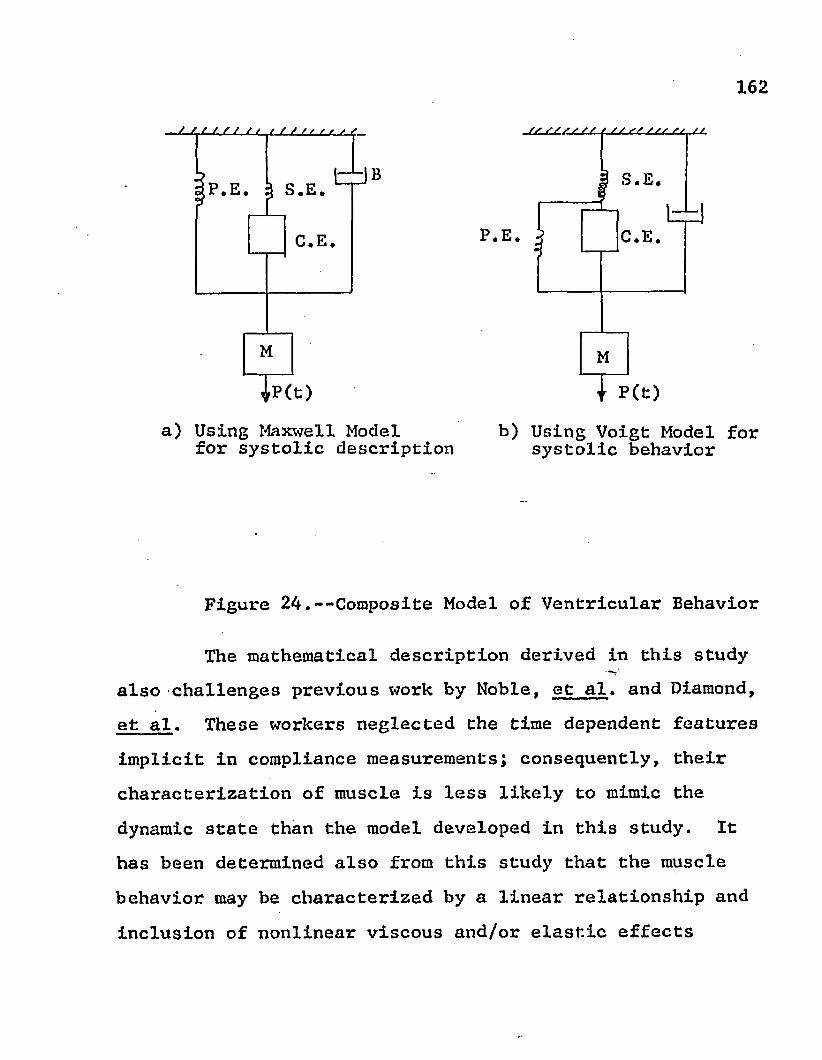
162

P.E S.E

C.E P.E.

S.E.

C.E.

MTP(t)

a) Using Maxwell Modelfor systolic description b) Using Voigt Model for

systolic behavior

Figure 24.--Composite Model of Ventricular Behavior

The mathematical description derived in this study also challenges previous work by Noble, et al. and Diamond, et al. These workers neglected the time dependent features implicit in compliance measurements; consequently, their characterization of muscle is less likely to mimic the dynamic state than the model developed in this study. It has been determined also from this study that the muscle behavior may be characterized by a linear relationship and inclusion of nonlinear viscous and/or elastic effects

163

contribute no significant improvement in model output (Table 18, Chapter VII).

It must be emphasized once again that the model developed here based on a least square error criteria defines only an equivalent model. In the absence of adequate theoretical basis, there is always the possibility of devising a better model description which can only be derived from further simulation experiments. Limitations of present measurement techniques which yield errors of the same order of magnitude as developed in this study preclude any further simulation. However, I personally am biased toward this particular model and feel that improvement in measurement techniques may yield a better fit using the present model. One strong reason for this particular bias is that comparable systems in fluid mechanics theory have been described using inertial resistive (viscous) and elastic components.

To devise a useful description of the diastolic behavior, it is felt that much more accurate measurements be used with the OMA. These measurements should more closely approximate the normal heart behavior and, therefore, must be noninvasive in nature. Also, they must be taken in nonanesthetized animals to quantitate heart function in awake conditions. Work is in progress to develop these

measurement techniques utilizing previously instrumented animals after their full recovery from the preparatory surgery. Bishop, et__al.67,68,69 have described techniques utilizing implanted piezo-electric crystals for dynamic measurement of internal ventricular chamber diameter. Indwelling catheters can be utilized for continuous monitoring of the left ventricular pressure. The surgical techniques for this instrumentation have been well elucidated (Rushmer^O), It is felt that these newmethods of measurements will provide more accurate data on heart function for normal unanesthetized animals. With this information, a better representation of the diastolic behavior for diagnostic purposes can be devised.

Discussion of OMA.QQRecently Mancini and Pilo07 described a procedure

for fitting experimental data using exponentials. Theexponentials may be interpreted as solutions of linearhomogeneous differential equations with constant coefficients.

89Mancini and Pilo use a digital computer to obtain the optimal exponents and the coefficients a^ based on the following multiexponential model:

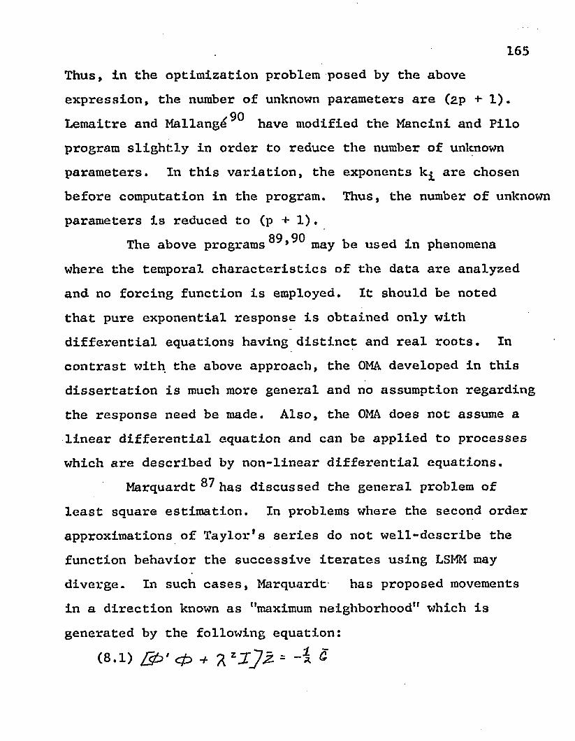
165Thus, in the optimization problem posed by the above expression, the number of unknown parameters are (zp +■ 1). Lemaitre and Mallang^^ have modified the Mancini and Pilo program slightly in order to reduce the number of unknown parameters. In this variation, the exponents k^ are chosen before computation in the program. Thus, the number of unknownparameters is reduced to (p + 1).

89 90The above programs * may be used in phenomena where the temporal characteristics of the data are analyzed and no forcing function is employed. It should be noted that pure exponential response is obtained only with differential equations having distinct and real roots. In contrast with the above approach, the OMA. developed in this dissertation is much more general and no assumption regarding the response need be made. Also, the OMA does not assume a linear differential equation and can be applied to processes which are described by non-linear differential equations.

Marquardt has discussed the general problem of least square estimation. In problems where the second order approximations of Taylor*s series do not well-describe the function behavior the successive iterates using LSMM may diverge. In such cases, Marquardt has proposed movements in a direction known as "maximum neighborhood" which is generated by the following equation:

(8.i) /& ' <p + ^ '■ J ' jz . - t e

166

where:X is the identity matrixG is the gradient vector

is the parameter change vector& 0 deviation matrix defined in Appendix D.

Marquardt®? performs an interpolation to calculatethe "optimal multiplier" at each iteration step. It has

87been shown that the convergence properties of the abovescheme based on equation (8.1) are superior to that ofdiscrete steepest descent. This method has also beensuggested by Fleischer**® under "Damped least square Method."

87Marquardt gives details of theoretical justification of themaximum neighborhood concept. However, in the particularcase of the DEPI problems, even for very poor estimates ofthe parameter vector, the convergence of LSMM were excellentwhen used in conjunction with discrete steepest descent.

87Therefore, Marquardt*s procedure has not been used in this dissertation in the development of OMA.

Meissinger and Bekey^ have discussed the principles of continuous model adjustment (parameter tracking) as applied to parameter identification. Continuous model matching adjustment is particularly adapted to analog computers and a number of researchers have applied this technique to a wide variety of problems. This approach

167differs from the one actually used in this dissertation in the choice of the objective function. In the case of para­meter tracking, the objective function is defined as instantaneous error (difference between actual output and model output at a given instant of time). Thus, in parametertracking corrections are made continuously based on this

91instantaneous error. Meissinger and Bekey x give theoreticalfifidetails of the method (see also Korn & Korn ). Parameter

tracking methods are conceptually related to the equationerror method developed by Potts, et al. and Ben. Clymer.^l

91As shown by Meissinger and Bekey x both these methods usefi Sthe same adjustment equations for optimization. Bekey has

recently (1970) shown the remarkable superiority of parametertracking over discrete iterative searches when the systemdifferential equations are simulated on a hybrid computer.The required computational time is considerably shortenedusing hybrid computation for DEPI problems in which the

65order and form of the differential equation are known.However, hybrid computations require interacting analog and digital equipment and are not generally available.

Bekey and McGhee^ point out that the stability of a continuous adjustment algorithm is very difficult to ascertain, a priori, and manual intervention is required to achieve a loop gain for rapid convergence without instability.

168While a completely digital computation algorithm requires longer time than the hybrid method, it does not require manual intervention.

It was, therefore, decided to develop a general purpose iterative program which could be used with tabulated data. This program OMA, does not require a lot of sophisticated equipment as may be necessary with hybrid computation. It is felt that the method chosen in this dissertation can be of universal use in physiological system simulations.

The OMA developed in this work is quite general in nature. It can be applied to any physiological system identification based on time varying input-output data.The identification problem is considerably simplified for phenomena in which the form of differential equation description of the process under study is known, a priori. Since the OMA has been written as a collection of sub­routines, It can be used with optimization problems where both the objective function and its gradient can be numerically evaluated (see Appendix A).

CHAFTER IX

SUMMARY

In this study a mathematical model of left ventricular behavior, specifically the relationship between diameter and pressure in diastole has been developed. The model is in parametric form and considers the time dependent aspects of the ventricular phenomena. The model is derived from computer simulations based on least square error criteria and utilizes experimentally observed data from normal closed-chest dogs. In the first part of the study optimization techniques have been utilized to develop an ’’Optimum Minimization Algorithm,” OMA. The OMA as developed in this study combines features of the available minimization schemes from literature to a minimization problem using the smallest number of functional evaluations. A new multi­dimensional search method called Reverse Golden Section Method (RGSM) has been specifically developed in this study for use in OMA. The method RGSM computes an optimal distance to be moved in a given direction for minimization. The second part of the study is concerned with the formulation of a valid mathematical description of the left ventricular

169

170

behavior. The shortcomings of the available analytical descriptions of the ventricular phenomena have been described and the needs of a parametric form of the ventricular model discussed. Successively more complex differential equation forms have been utilized with the OMA developed in this study and ventricular data to derive a parametric model starting with a linear first order description of the process and progressing through various nonlinear equations. It has been observed on the basis of simulation experiments that the ventricular filling is described best by a second order linear differential equation relating the left ventricular diameter to the intraventricular pressure.

Based on the parametric model thus derived, the study attempts to relate the ventricular phenomena in terms of viscous, elastic, and inertial properties. It has been shown that the parameters of the proposed model are invariant within the accuracy of present measurement technique when the period of diastole is constant. The model has been tested by administration of known positive and negative inotropes. It has been observed that the inotropic changes reflect in variations of parameters of the proposed ventricular model. Attempts to quantitate the effects of the administered drugs have been made and the need for maintaining the period of diastole constant have been indicated.

Inadequacies of present instrumentation techniques and the need for more precise measurements have also been indicated. A composite model defining the ventricular behavior both in systole and diastole has been predicted.

It is hoped that with better measurement data the parametric model developed in this study may be used in quantitating the differences between a healthy and a diseased heart muscle.

APPENDIX A

COMPUTER CODING OF THE OMA

172

COMPUTER CODING OF THE OMA

This appendix is composed principally of a listing of the FORTRAN IV coding of the OMA as developed in Chapter V. The complete program, as listed, applies only to the DEPI problem relating to the ventricular pressure-diameter relationship. No changes are required in the application of OMA to other DEPI problems using the least square error criteria. Possible changes in the choice of a particular minimization method may be made by modifications in the MAIN program. This modification may be required in minimization problems other than the particular DEPI case discussed In this dissertation. A brief description of the subroutines that may be modified for use with other minimization problems is given below:

Subroutine SOLVE- i

This subroutine solves an assumed differential equation form using the Runge-Kutta Fourth Order method.This integration routine (Runge-Kutta method) is available as DRKGS in the IBM Scientific Subroutine Package. The subroutine DRKGS is in double precision arithmetic and has been used here with h, Interval of integration, of .001.The library subroutine DRKGS requires two explicit subroutines FCT and OUTP. Subroutine FCT provides the differential

173

174equation description and subroutine OUTP is used to save the computed response points YG. Other integration routines may be used to solve a given differential equation form by modifying the SOLVE subroutine.

Subroutine SQRERRThis subroutine computes the objective function

F(£) at the given parameter vector "A with the assumed differential equation. SQRERR has been coded here for minimization using the least square error criteria. For other choices of the objective function, this subroutine must be modified.

Subroutine APGCAPGC computes the gradient vector T*(K) and the

deviation matrix based on the least square error criteria for a given differential equation form. For other minimization problems using other objective function criteria (different from least square error) this subroutine must be modified for calculation of the function gradient.

Description of Input Variables and Data Preparation for use with OMA

Due to the pecularities of the OSU computer centerset up, the turn-around time for tape input data is ratherhigh. Therefore, the identification of the pressure-

175diameter relationship has been carried out using two steps. The pressure and diameter data derived using the program described in Appendix C is punched on IBM data cards. These cards are then used with the OMA to derive the differential equation form. This allows for a significant improvement in turn-around time once the pressure-diameter data has been digitized permitting several computer runs to be made in a short time. This is quite useful when several differential equations have to be used and the simulation depends on results obtained from earlier computer runs.

The input variables used in the computer programare as follows:'

AH *■ Vector of upper limits for parametersAL ** Vector of lower limits for parametersR, AO, 83 Vectors for intermediate storageAlGRAD a Vector of gradient of the objective functionPHI =* Deviation matrixA =* Vector for parametersYT = Vector of experimental output variables. In

the study, these are the diastolic diametermeasurements at every n*8 msec, interval.■where: n “ 1,2, or 3

YC “ Vector of computed output variable. Samenumber of data points as YT.

p

KKK

ICQ PRMT

ND1M

Y, DERY »

NUMA

IX

NP NT

Vector of input variable. Same number of data points as YT.A counter used in OUTP subroutine to keep track of data points YG.An integer counter for intermediate computations Vector required by DRKGS. PRMT supplies information about initial time, final time and the interval of integration to DRKGS.(For further details see IBM Scientific Subroutine Package.)Number of first order differential equations as required by DRKGS.Vectors describing the given differential equation as required by DRKGS Number of unknown parameters in the given differential equationAn integer required for generation of uniform random numbers by an IBM library subroutine RANDU. (See Scientific Subroutine Package for details.)Number of data points•An integer specifying the number of independent searches to be carried out using Random Search (RANSER).

177G " A constant specifying the accuracy in

parameters for use with RGSM.The format required for reading in all input

variables may be obtained from the FORTRAN program. A typical set of data cards is provided with the program- listing (OMA) which follows. These cards will provide the experimental results described in Chapter VII with the second order linear differential equation.

n » (, r: y! I 1.0 V .-!

0 9 i t n.t. a a_________(yLdli^J~liLI.J.vj.L^o^.l^A31J>!M_____________

i'iHSl £ 0 2 * 9 ) El JL f >lf*i ' O.Q.T I_JJ. J.... QO.U/.O . J.D. * „ W.0S )A l ._

V2TT 0 1 0 9 * 1 * 0 3 * Vf) ri I ______________________________J_______ _1:J2S.2.S_____________

'?Z\ I U 1 0 9 ( 1 * 0 • 1*1 • { S A T ! S - T ) } 3 I jt-jjab!d.u-!>L*.avj.ij>rjai^ti.iiiicjiA/L-ii.uni-iTvs:i_nav.'a..

( w n s * iH d 1 (JV'dO 1 cIN 1 Vh(h-I) DVldV 11 V 3 O OI T_Lijjy;n.sLLu-iiv^iw‘jjw,ti\LLx.ij.uastJi/.y-JD.v.a _—

S =HHS ______________________________________ QZ.Q.0.1 aaO-L

{ I ) A = C I J3AVSA 5V__________________ LlLQNiJLi=I_S.tea..Qri_________( V 4 1= I * t 1 ) J.wy d ) ( £ 0 2 4 9 )3 1 n f f i

-..(J/_‘_Lr_L‘ ..( JUJLU'dd.)J.LQ^_Li.)XliGM„( WICM* T - I 4 I I ) A ) ( K O Z ‘ 9 JEl in iM

_ L I ) A .LUn-ZL<LLLL'lR '±SSiVlVA I V I I I N I ClV3>l 0.

Id t lU iU .L U L L d J J S o Y .19. ) r.LLJ.1LU_________( hw* 1= i M n hi ( io:< 4 r ,)civ3>i

L = L4 ( I ? ia ) (_£u z t p ) 3 i i j f t clIM* T = I * ( I ) 1 A ) ( £ 0 2 4 £ UiV3>i

ciW( 20? fc 9 ) HA HIMdi->( 2 0 2 4 £ )C!V3>< 0 0 0 2

S lM U Id 1 V l N 3 WI>l5rfX3 0(.ViJHt'i4 T = I 4 ( I ) V ) ( £ 0 7 . ‘ 9 ) 3 I IV tM

(\V wnN 4 1 = 1 ‘_LJJ V ) C EO? 4 9 ) fJ V 3>1 ] 'd0103A 9WI1>1V1S V C1V3VI

W I O W / O * I = ( I J A W 3 0 !-..; t-fiMt r = [ y? na( vwnw 4 I = I 4 { I )'JV ) ( £ 0 2 4 9 ) 3 J. I VIM

V31<_t v wriM4 1 - 1 4 ( r 1 hv ) t £ 0 2 4 9 ) 3 1 r v:/r

t n i!v*> ( l o ? . 4^ iav .3^V .TJI S 4 a t £ 0 2 4 9 ) 3 i I VIH

_____________Vi-JiUiLi.a LLQ2l.S.jmi.3.VL.1 U 4 X I 4 VkYlM 4 Vi ICIl'J ( 2 0 2 * 9 )31 IV ! M

1 M4 X I 4 V 11ON 41'11 f.H ( Z O Z 1 g )Cl V 3 >1( fl ’ S X d S 4 i ' 1 JIVMVIOd £ 0 2

( M A 4 .__< H.V!-i>in3 2 0 2(O'STzfSUVWHCl:! TOZ

I = S Nt S) 3 AVSO 4 { c) 3 AV S A/ Z WW0 / NtJWNOO

!•! I C1M 4 ( S) AM 3(14 ( S) A 4 f l!v>M/£T 1 3 / NPH-MIOClM 4>l ;014 { 0 0 1 ) OA4 ( 0 0 t ) r!4 ( 0 0 1 ) JLA4 ( 01 J V IMUt-IWUO

4 (OT )0 V 4 tQT 1OVMO4 ( 0 1 4 00T ) I l -M* ( 0 t ) M4 ( 0 E ) *1 / 4 ( 0 T UJ V M n rSr-‘3 K f ni z-u h i-vj ti*iv3w n a n d H i

8 n

179* OU' 1 1 0 1 1 = 1 , IV'UH A

1 1 0 1 FACTOR-* FACTOiM GRAD ( I ) * G R A 0 I I )------ F/VC tcj’r = n s r r t* ( f a c t o t t j----------------I F ( F A C T O R . . G T . I O O J G O 1 0 H O B

----------------j-pnrr^X TnTT . G T . T ) tTO'“ TO 1 T7T>------------------1 4 0 0 DU 1 1 2 0 J = 1 »tVUi iAr— a o (~i i j r * A - m -----------------------

I F ( A 0 ( I ) . LT . A L I I ) ) A O (1 ) = A L ( I )------ A i m -7v~rr)----------------------

I F { A 1( I ) . G T . A H (1 ) ) A 1 ( I ) = A H ( I 1TT2 6— corrrTwu H — — ------------ — ------ —

CALL K AWSE R I I X , AO , A 1 , MUMA, 0 1 , S U H , 1 )--------------- I 'F d T “ S"u F T S I ^TTH O TTT~u"“TO TIATi-------

S=SUi' i

1 1 0 3GO To 1 1 0 0 DO 1 1 0 4 1 = 1 , MUMA

1 1 0 4 GKAUt i ) = GRAD ( I ) * ( - 1 )CALL UUAO ( SUM , GRAD , DUMA , MP , AH , Al, , M )GO U ) 1 0 5 0

1 1 2 8 CALL R GS M( MUMA, GRAD, S UM, C , M , A H , A L )10 5 0 I F ( SUM . E U . S ) G0 1 0 1 4 00 ■

SUM=SGO TO 1 1 0 0

1 1 4 0 l\'S = r;S-i-lW K 1 T E ( 6 , 2 0 3 )SUHW R I T E t 6 , 2 0 3 ) ( A(J ) , 1 = 1 ,MUHA) 'U KI 1 h t 6 , 2 0 3 ) ( Y C ( I ) , I = 1 , H iJ 1I F { MS . G T . 1 0 ) STOP 3 2GO" iD 1OO0EMUbUiJKuu i i i -;t h i i i i , if l U t i o jI M P L I C I T R EAL- t i ( A - H , 0 » Z )T J iT - . 't^ T D r r r n r F r r r r r r r , y t t t t jCUMMOH A 11 0 ) , YT ( 10 0 ) , P ( 1 0 0 ) , YC ( 1 0 0 ) , KKK, KGTF ( KKK . h G . 0 ) GO i u 10Z = P ( KKK)-!- ( (P 1 KKK-i-l ) - P (KKK ) > / . 02 0 ) * ( T - ( K KK - 1 ) * . 0 2 0 )

1 0 0 U E K Y l 1 ) = ‘M 2 )DEKYt 2 ) * <A ( 4 ) * 2 - A ( 1 ) * Y ( 1 ) - A ( 2 ) * Y ( 2 ) ) / A ( 3 )RET URi'i

10 Ji!i!iijiiI

a. I

n ;

rx!

GO 10 1 0 0 ,DEBUG SUDCHKtriu

180SUtfKUUT INE SOLVE t P Jli-.T , Y t DERY , MDIM )~iti p c rc T i" ‘"k 17 n r vn - r j --------------------------------------DIMENSION Y ( 5 > , D e K Y ( 5 ) ,PKi iT (5 ) , AUX ( b , 5 )

TOm-iOTP A T V 0"r,T TT UTO V,'PTrOOT,‘ YC T'TUOlTiCI;K7 iCtr C()MM fJW / C h M2 / Y s A V E ( y ) , US AV E { 5 ) 't t o -t o s v” 7 C t t u f t t T'TTK a - - - - - - - - - - - - - - - - - - - - - - - - - - - - - -EXTERNAL FCT, OUTP

“KKK^tT--------------------------------------------------------------------------------CALL D R K G S ( P R M T , Y i D E K Y , N O I f i , I HL F , FC T, CIUTP , AUX)

~C RE'S TUKif'"Ti Ic lJErl G it! Al: _C(.'!TT"*Etl'YS'“ t)f:""Y—AWO~U tt RY‘“ { ~ i H tr'T N l T l A'tr'CUivf):-':^)- 11 DO 5 7 L = 1 , M D I M

----------------Y tt '-J ^ U A -V r-t L“ >-------------------------------------------------------------------------------------------------------------------5 7 DE KY( L ) - 1 . 0 / NO I M

----------------1 P ( ' I'M L'F'TG 1 Tl.'O") G0-'1 D—2-3U-------------------------------------------------------------------------------------------59 RETURN

~23Q- - - Pi<‘ r t 5 7 -J HtrF- - - - - - - - - - - - - - - - - - - - - - - - -- - - - - - - - - - - - — ---- - - - - - - - -A55 FORMATC ' 1 , 1 JHLF *= ' i I A )---------iTH-'mrrM----------------------------------------------------------------------------

DEBUG SUllCIUsEMD ~ ____SUBRUUT I ME O U T F I T , Y , O H k Y , I HLF , NO I i - i , PK;-iT )nr?LTCT‘l Is t: A L^tTT/'-h , u - FTI) I ME MS I UN Y £ MD I :•)) , D c K Y I H D I h ) , PRMT ( 5 )------ CYYrir.lu;irin'10')7YTlTn777P'nT;77y7YC’(“lWr77<T<TL'7KO :I F ( { T-Pfti-iT ( 1 ) -- ( KICK *2A *P ROT (3 ) ) + 0 . I t ) - 5 ) . L T . O.OJGt! TO 69

“CTCKfC“rS “ 7Y” CC :UT71"!:'! TTCtrTfRiTT3— R7YC C~u f ~ T IVc 'T i U :ToCB "Up—Y7H*~S~ 0 R“ Y C 1-$~XT rTtrJ7 KKK=KKK+1

--------------- iX 't iG s rm ^ Y i^ rr----------------------------------------------------------------------------------------------------------------------69 RETURN

--------------- [tet;ug~ s d b cm ;-----------------------------------------------------------------------------------------------------------------------END _____ _______ _________

-STlB^0CTTT^-‘--SCRF7CrrYC fT T V STE:i h ,1717)” '“ *" !-------------------------------IMPL I C I T REAL* 8 { A - H » (J - Z )[)Ttte o s r o r 7 c 7 i w )7 Y T iT (K 0 7 'E r iw r ;? n --------------------------------------------------S= 0 .D 0 ~5 J =T7N-------------------------------------------------------------------------------------------------F:( J , L L ) = Y C ( J ) - Y T ( J )

"5^*S+FCT7H ^ F I j , LL )'■ RETURNEK'DSLJBROUT IMF APGC IN , KK1 , GRAD , PHI , V AL )I M P L I C I T K E A L - a ( / - rl ,J.J-Z )D I ME MSI CJM E I 1 00 , 21 ) , PH I (1 0 0 , 10 ) , GR AD { ). 0 )C On HUM A ( I 07 , Y t ( 1 t;0 ' ) 7P * ( T0 0 ) , Y C l ToTTTTKX k ,7;u CfJi !H UN / C i i f-i 1-5 / PKHT ( 5 ) , Y I 5 ) , D f: RY (5 ) » Mf) I H

T n -7 fE T o 7 2 o 7 o 7 '

2 0 1 0 FORMAT! ' ENTERING APR GRAD ROUT I M E ' )C A L L ~S l7L VE rPlCTT'i Y 7'1 tTRY77-1TV777)CALL SORERR { YC j YT , VAL. , I: , KK 1 , 1 )

181------------ l7RIT F V trr iO T T i:LL~V7.'L'

W R 1 T L: ( ( j , / i 0 3 ) t A C I I ) i I ] = ]. , N )-------------------- d d ~ i . cn~"T = ry u ---------------------------------------------------------------

ASAV E = A ( I )-----------------------d'e x t t^ T r m y T o o --------------------- ------------------------------------------

l F t A ( l ) . E Q . 0 . O ) D F L T A = . 0 0 0 0 1 1-rj---------7 STGTT=TSl C ’ - T - IE ) ------------------------------------------------------------

Al 1 ) = A SAVE I- I S I G M * l ) E L T A-----------------------ctt trL~—STTrv tr i p R n T T Y n re k y 't n d 'H t )-----------------------------

LLL= LLL- I -1---------------------- C A T n r™ 5 T 7 ^ T 7 rrn T T Y T T 5 'U rrS P T E 7 in n T C rn ■

AO3 FORMAT! 1 A 1 »1 P S E l 5 . 7 ) 3TT3 F'CJRT-I7\Tn SUi-7STFIT T 2 " , ^ T T P 'F l i r m

A l l ) = A S A V E----------------------- 1 T f T S 'lU r r rG T7(JTGTT7 0 T 5

0 0 10 1 J = 1 , K K K----------mTn jTTi^rr-rji i r-ircjy^ i + r)T7T7 mnrnn'

101 CONTI MUET5D - J A T ^ T T N 'GHAHt I ) = 0 . 0 D G - 3f7_ !_ T _ ,, RT< -

3 A GRAD I I ) =GKAOI I > *P i l I I J » I ) * E ( J j 1)---------------------- VTP* TTE't 'S T 'f T n T G K T V iri l “lTl~=‘r ’iTT)--------------------------------

A 7 7 FORMAT! 1 1 , 'GRAD 1 , 1 P5E IB . 7 )----------------- ---------(7K 1 T £ - ( -fyy/fQ Q-)-------------------------------- -------------— -------------------------------

A 0 0 FOKMATl ' E X I T APP GKAU R O U T I N E ' )--------------------- T;E i UKM------------------------------------------------------------------------------------

END-----------------------Stft iY-tttfT"!"!? E—1:vAt t-PAtE < ■AnrrX t A? i 1 t t : I r r r I')----------------------

1M P L I C 1 T REAL * 8 I A - H t 0 - Z )■--------- tr]TTET'TS'rrjN“A~<'rcr)_t**AiTf70tT'Arir<‘l'0)------------

DO 3 0 1 1 = 1 ,N ..---------------------- CTTCL- i<AT1Dtr( ]“Xa T Yt YT L-)-----------------------------------------------

Al I ) =AL 11 ) h- t AH 11 ) - AL I I ) ) * Y F L-------------------- r r i ‘7: m —ri£ o ~ o -vo -rrrD -^c rro T rc -trcn ---------------------

3 0 1 I X = I Y RET0Rpj ------------

‘ END

------------- WtTRO'CJTTTfE "L'STTiTTTT^TaC I'TSTK rAirTTJ-lTPH TT i’O-------------------------------------------I M P L I C I T R E A L * t t I A - H , 0 - Z )fjin e:ns7 nr? prrriTO orro'T rrrrrrn T z i ittitte m p i xcrrtTnTTE iw srru rrr;

1A L I 1 0 ) j A H 1 1 0 ) , X ( 1 0 0 , 1 ) , A 0 { ). 0 )ctfiT tdtt" ATnrrv y t t i tttti * r rn' p tg t,~ t c t to u t t kisKttcit-------------------------------coriHOiv* / C ‘- ' ' i 3 / i j Kirr i , y i s ) , o e r y i s ) , h d i hWHiTtJT (7,2f»dT .....

£ 0 0 F U K M A T J J E N T E R I N G L E A S T S Q U A R E R O U T I N E J J _______________________________

33 7. ( 1 ) = ( — 1 ) :'*:R I I )

182" i E M p n , j P o . o ** ......

l)G 2 2 K” 1 t HICKt ?. T O T ( 'i^ T ) '= T H - iF r n T )+ p r r r n c r i ' 'r * 'P T r n ic r J ) 1—

DO 300 I "] , li'lK{ 1 ) = OSOKI (1 E.-iP ( 1 , 1 ) }Z ( I ) =Z( 1 ) / K ( I )DO 300 J * l , N "FB«DSORT (TEMPI J , J ) )VFinPTTTJl = TEMP ( I ,0 ) 71T1 B*K"CD ) "

300 CONTINUE~C TP I he DT.-itHS roKs uF *l ciTFH A/vO TTJ7TP Af-Ci: cTTXTGTTD MTTdTF1? CALC /VRr, 19 CALL ARRAY (2 , M | N , 10 , 1 0 , TEMPS ,TEMP )

c a l l sTr,LiTt¥crp3'7T7f:'>7Ks)...............I F ( K S . E U . l ) S T O P 907 tJb lb'o "I = rCN

100 2 ( I ) = Z U ) / R ( n-------- ITlTTTtl" F 7 ^ T o T r Z T D T r 7i''rcn~”“ ------------------------------------------ -

4 7 6 FORMAT! 1 1 , 1 Z 1 , l P 5 E 15 . 7)‘C’STWt CljI;i’RTTED_ Z'_\ rALirF"S"”'Fu?rTDT'GR'E"”lTSTr~17']~C'ASF~UF""R7n'TG'E '77T)r7VT'r07'TS“

DO 3 4 1 = 1 , W-------------- rE7iP3rt‘T)"=z_n " j----------:-------------- — ----------------------- *--

AO ( I )= A ( I )3*4 7\TTT=TTCn T J T Z m -----------------------------------------------------------------------------------------------------485 CALL G R A D U ( A , Z , N , A H , A L , K ) --------- 1 F n T.T )T, D p q— — ------------------------ _ _ _ _ _ _ ----C COMPUTE SUM SO ERROR '--------------C7CLTL STSCVETPRMTTY'jTJ’EKYTWDTF-V)---------------------------------------------------------- :-------------

CALL S O R E R R ( Y C , Y T , S I , X , K K K , 1)ITTS TY LT «iC J GO 1*0 49 4 ’

C REDUCE THE COMPUTED Z BY REPEATED HALVING Ak’D RERUNNINGC RA’L V"E '"TRT** C OD FOTE D~Z~A fT T T ? ^ -----------------------------------------------------------------------------------4 9 6 0 SCAL E = 0 . 0

DTT' 44' ' T^TTT'T TEiAP3{ I ) = TEMP3 ( I ) / 2 . 0

-------------T T T T ^ T E T T F T m ------------------------------------------------------------:---------------------------------------------A( I ) = AO (1 )-t-Z { I )

_4 7 f s"C7\rE^src"AT i r * z r i T s r m ---------- — ---------------------------11: f SCALE . L T . . 3. l‘) - 3 ) GO 10 496

ttxtjttp O T F ^u r-r* s c * “pkrotv*****-----------------------------------------------------------------------------------------------GU TO 485

4*9*4 TrRTTE*(Tr72*229--------------------------------------------------------------------------------------------------------—222 FORMAT! ' -CONSTRAINED MI NI MA BY LEAST SUUARE ME 1 HOD' )

WRITE! 6 , 4 0 5 ) S4 0 5 ------POKnA"T'(**' •“ ' —= ~ ' v 1 RE t^n rf-)----------------------- *— ---------------- ----------------------------

WRITE! 6 , 2 0 3 ) ( A ( I ) , 1 = 1 , 1-') 2T)*3 l-URMA'TC1 ' t 5F'1"5”;8 ')---------------------------------------------------------------------------------- ;------- ;—

H= 0

496 M=1

183------------------ D 0 ' “4 6 I =T 7N '

4 6 A( 1 ) = A O( I )------------------rVET'UR'R------------

END

CCC

S U Li k n u r r N t S J ,'i t / (A , U ,; s' , KS) I M P L 1C I T R E A L * 8 ( A - H , U - Z )Dli-lfciMS JON A ( 1 ) , Li ( 1 )

FORWARD SULUT I Uiv!

I U L = 0 • 0KS" 0J J = -I'JDO 6 5 J = 1 , N

-------JJ= J J+N-i-1 in b/\ T5 I T= J J - J

u t T 3 o r= j , ftcT ■^EaT< CTT“ F OTT-Ti-AXTR^ TCiT] TN“ 'CU'L‘OT-riT

r F i m ------------------------------I F ( D A D S ( S I C A ) “ D ABS ( A ( 1 J ) ) ) 2 0 , 3 0 , 3 0

20 B 1G A = A T I J ) ‘ ~ ~IJ i A X = I

~3o coirriKuir

c— C‘

c TEST FUI< P I V O T LESS THAN 1 UL FRANCE t S I N G U L a R Li A I R I X )c

I F ( D A B S ( B I G A ) - T O L T 3 5 , 3 5 , 4 035 KS= 1

kb i GRnc >c J N 1 t KCi lAl'JGb KU1.1S I F R'bCbSSAkYc

4 0 ~IT=4J -i- i'J - ' { J'-'2 ) .......I T = I clAX-JDO 50 K = J ,M1 1 = 1 1-t-M

SAVE- At 1 1 J lY T T l) ='A“C1 2 1 At I 2 ) = SAVE

D I V I D E EUUA'f IGN BY LEADING COE FF I Cl L: M'I

5 0 At 11 ) = A ( 1 1 ) / !i 1GA SA'vn=i i t ' i i - i r x ) ....fit In AX) = D ( J )fTT I t ) V, s A VIE7 u 7 G7\-----

184‘TT TUTTTIT17C I 'F ’i'J E'XT " V V\ IIT7\7TL~F

■<rc

X ”

)'“ 5 ?'i Tr)755“353 1Q S - N * ( .1- 1 )

DO- 6 5 ” T X«HYVM--------I X , J = 1Q S + I X ITsTFTX----------DO 60 J X ” J Y t N

I X J ' X - N - T 71X - r M - x -J J X = I X J X + I T

■ 6 0“ A T l'X a x r =077 ) X0 X-)“ t V ( I X j -) :;rA-( ;rjX -}- j— 65 B ( 1 X ) - fi ( 1 X ) - ( B < J > * A t 1 X J ) )

BACK S O L UT I O N

7 0 N Y - N - l] ‘I - N*N DO 8 0 J = 1 , W Y

~I A = ~I T—J ] 5% = M — J

80

] C “ NDO 8 0 K" 1 i J _______

T f I [$Y- B ( ] lV) - A C I A ) *B~( 1 c T ] A = 1 A—N ~IC«IC"1 RE 7 URNI: I'lDSUBROUTI NE ARRAY { MODE, I , J f N , M , S , D )T^u^rx'rr-KCAr^rni^HTo-zT------ —

D I M E N S I O N S(1)tD(1)N I = N — I

trcTT

CTCC

TEST TYPE OF CONVERSION

I F ( M O D E - 1 ) 1 0 0 , 1 0 0 , 1 2 0

CONVERT FROM S IN G L E TO DOUBLE D I M E N S I O N

100 I J = I * J i - l .7F.= N*J-U..DO 1 1 0 K = 1 , J i7M=N.vi-Tir DO 1 10 L = l . , I

110"cc

120

JJ= 1 J-lNM-NM-l 7/(770) = ST) jT GO TO 1 4 0

CONVERT F R O i i ' j m U B L B

I J » 0

TO S I N G L E D I M E N S I O N

185--------------Rn=D----------------------------------------------------------------------

DC) 1 30 K= 1 , J--------------D t n ; 2 L i - r - i T i ------------------- --------------------------------

1J = 1 Ji 1-------------- RTTSTTIVI---------------------------------------------------------------

125 SI I J ) - - D ( i'JI-i ) O U " M i = Kf-rFr! I----------------------------------------------------------------c lt£*Tt:) KM----------------------------------------------------------- -----

END------ suirrTom"} n^^TfnD rrxT-rrrr^AtrmrTTii----

I M P L I C I T REALMS ( A - H , G - Z )DTT-TB'l5TDi>r~AT20TT2“f 2 UJTAT-I T 2 D-TTTa^tYtT)' H= 0 DT]_ _ 1„ T i T „,.i-------------------------------------------------

IF ( Z ( I ) . G T . O. OI GD TO 2-------------- rF 'O T T IT T G T . ATTTTTCR'rTD “A----------------------

GG TG 32 rn~ A i 1 7 " 'vgt ."“ A T rn y i c r r to“ 3“ “ --------

GO TG 1

3 -------------A ( ' r ) - ^ A t r ) = x - t 'n ---------------------------------------------------------------------------------------------------------M=M+1------ Gtr-TtJ— 1--------------- :---------- ;-----------------:

A 1 F ( A ( I ) . M E . 0 • 0 ) G 0 TO 1-------- z r m ^ c n r T T F n ------------------------------

W R I T E ( 6 , 1 0 0 )TOO"------FT)kTiTrfr'r ~ F v V i O \ 7 T E T c T ~ V T T ' I ' J F " 7 T T T T K T F T T T ' “TfTTS PU J N I ' T1 CONTINUE “ k ETO^ :

ENDSUi iGUUVlNt: RANGER I J X j AL , AM »N jl'tT jSUi-i j IsR ) "I M P L I C I T REAL * 8 ( A - H i 0 - L )DO M EN Sl ON A L 110 ) , /: H I 10 j , X'( 1 0 } , E ( 100 , I )COMMON A ( 1 0 I i Y T ( 1 0 0 ) , P ( 1 0 0 ) , Y C (1 GO) , KKK,KO

. COMMON / C / - T 3 / P R mT ( 5 F» Y'('fj') r DE'KY"T5T, MlTTi-1 1 F ( K R . F Q , 1 ) GO TO 50 CALL K AH P A R ( A » I X i A H , ML t M )

5 0 DO AA J = 1 1MAA “ X ( j f = A ( J J

CALL S O L V E ( P R M T , Y , D E R Y r N D I M )CALL*"S(,RE RH f Y C Y T , S U.-itf XK;<7TJDO 3 5 J = 2 i NTC AL IT t ; f \ i ■<i ' /• i T7\»~ I~K ?7-H j AL »M )CALL SOLVE ( PRMT »Y , DEP.Y »KI) 1 M )

■— --- r/\L_L'~S"(Ta?rT'(YC;7YT7\STJia‘','E7TiaT7TII F ( Si lMl .GT . 5 UNO >G0 TO 33

--------------- SUM OS 5 0 P. 1-------------------------------------DO 6 0 1 -• 1 11’!

-770--------X T T T -T tH " )------------------------- -- ----------

186------ DU"TK3-*r=T71T “ ------------------------*-- ------66 A( 1 ) = X( I )------------- R .R 7 T ^ .a -T 2 r r r t 7 r ( T .j----------------------- ------------------------------------ — ------------

WR IT I:( o , 2 38 ) MT YTi---FURTT/TTn •_inr,7rirTTTr>: TTP'pETITTT'I238 FORMAT! 1 ','THE AI’UIVE COE F F IC I ENT VALUES ARE AFTER',14,------TrR7T7'"iTrj7“ 'rFar7ir!r» i :--------------------------------------------

SUii= SIJMO-------■R'ETUrtT'i" * —

ENDSU6 RLiUTTiTE KUSi'i (Kr, GRAD-, V AlTTCK,~iAT aK7ALT IMRLICIT REAL-8(A-H,0-Z1

---------TJTiTFi^ j'GTT_ GlVA[JTi:n-yV7rSl lTT]Tr.;STTT)lT CSTTOTTTJS'(ll)')''r7YaTTO )TI F ! 29 ) j E ( 1 Cl0 i 1 ) , A IK 10 ) , A L U 0 ) , X ( 1 0 ) , XX ( 10 )------ ciFTf;TGT'7_7riT(TT,"YTTiT.rr)','P'a'oa) rvccTOTn'TTsicirrrcGT" :COOHON /Ci-W'13/ PR NT t 5) , Y ( 5 ) , DERY (5 )IDA I A F/ . O rS'7TT0 , i . 66T2T75 , ■’rr5c>T7 .56, 12. 5"4‘y2 O.oT Vlr'TTb-t, :>195 . 1 6,157*96 , 2 62 . 2 1 , 6 3 5.26 , 722.53 , 1 1 9 9 . 3 9 , 199 0.9 8 , 3 3 0 5.02 ,

------2'34TT6T33T9 iT)'7T3U'i* 1 V X Yo V T T Y Z3 1 9 0 5 6 2 . 6 2 , 3 1 6 3 3 3 . 9 4 , 5 2 5 1 1 4 . 3 A / *

SUMS 0= VA L-321 K - 0 . O'-----------------------------------------------------------

DO 1.26 1 = 1 ,NTZ4-- -R -R f-'GFTTU (rr-GPv'ADT II------~------------------------------------

R=l)SUKT(R)---------d-q i2.rro“ ‘]'=rT_rM--------- ---— — ---------- “ -------------- -------------------1240 G R A 0 ( I ) = G R A 0 ( I ) / R Tf. ( R .__G T .vr; T n GT3_ Tt_ 1-2t)------- . . ----------------

DLAMDA=C-------GU_Tir^'7-------------------------------- ;125 DLAHDA--C-R

------------ T T T D L7v~ D 7 r T G T 'r " n iV r A F U 7 {^ T '---------4 7 K=14T5 nO '~Z7~T = T 7 N

X( I ) = ( - 1 ) * LI L A i-i f) A * GRAD ( I ) * F (K ) / r o - r n - 7 n - n -------------------------------

2 7 At I I = At I M X ( I )S I<FlT= SU'rrsoCALL G R A D M ( A , X , N , A H , A L > K R )

-------------T FTl<7T7ETr.7n'Gn 'T 0 —r 2 ’5~~L = K^ a l l "STcn7ETP7FTT7Y'7n E XYTTliT F T )CALL SOIiEKR ( YC , Y T , SUi-' .SO,F , K K K , 1 )I p"n^ . 3T H7= 3GfJ TO t 3 0 , 3 9 , 4 9 ) , L

T 9 ' iT rs T M S in GT'; S I"TGW TCT3 25 3 on 7 1 = 1 , 0

187

7 BS< 1) = A ( I ) S?=SUHSO

8 K“ K + 1 GO TO 4 8

30 Sl = SUi-iSUI F I S I . G T . V A L ) G 0 TO 55DO 6 1 = 1 , H

6 AS( I ) =A ( I )GO TG 8

4 9 I F ( S U M S 0 . G T . S 2 ) G 0 TO 31S ) ~ S 2S2 = SUilSUDO 10 J s l j i JA S t I ) = D S ( I )

ro b s r m r r n r rGO TO 8

3 7 . Dn~9"~r="lTW9 At 1 ) = AS ( I )

V A L - b IW R I T E ! 6 , 1 1 1 )

... m hUKi-iA 1 I 1 A 01 NTHUM FGUivD 1 ) RETURN

31 N 1 — !\“ 1S3 = SUMSO

.... STRFRsSUMbODO 1 4 1 = 1 , N

- -171 X ’S T T ) = A t J JC cs AND AS ES TA B LI SH THE UPPER AND LOWER BOUNDS RESPECT I V E L YC Dll USUAL r J !;>uK'AlX 1 SEARCH ACCURU1WG IU K i t h c k 1■it 1 HUD1 67 UEL = DLAMDA*F ( K- l . )15 J F= 13 DO 1 1 = 1 , M

' "x (_rT=D iri:= -g t<A irn r ~AO ( I ) = BS ( I )

1 At i i = US I i ) + * ( i )CALL GRADM( A , X , N , A H , A L , K G )

— I f {"KG1 rt"Tr*T r )"tn5i-,i t i izz —DO 11 1 = 1 , N

■ ~n — ' ITS'l"!) = 7 f( 'IT ....... ........ " " ........... ...................... ............ ..CALL SOLVE (PR: -1T ,Y,0EKY, l» in iM )

1 ' 'CALL'"St-'itE EK I YC'i Y 1','S Ur.2 i'E"','KKIs, 1 ) ......2 IF t J F . E O . N D G O TO 59

Kr- K— 1— 151i irwurA'MU A"-r'( iC—1“)-----

I f : ( SIJN2 . G T . S 2 H it) TO 61

1881 ’ DU' I 7 " J = ). ,Tr

AS ( I ) = RS ( I )....... T ? “ B s r r y - D s t r r

S2 =S U U 2SRFO= S2GO TtJ 3

61 DU 10 ] = 1 ,MC S ( I > = D 5 ( i )list ] ) = i is T i )X( 1) = ( - 1 ) * U E L * G R A D ( I )AO( I ) = I-S ( I )

I B At I ) = AS ( I ) + X ( I )SR F i i =S 2SUii2 = S2

' C A L'U ‘ ' G ' R ' A ' ( A , X , *177TT; A H 'K 'G T """"J F t K G . E 0 . H ) GO TO 1 2 aDU l v o 1 = 1 i rJ

1 9 0 B S ( 1 ) = A t I )CALL S t.i 1. VE t P R.Ti , Y , i'«fc RY , i•!f) 1 n )CALL S 0 R E R K ( Y C » Y T , S 2 i E i K K K i 1)

' ““GO Ttf” 2 " ........""59 W K IT E ( 6 , 3 7 )

— ~ r r — f g k ;-u \ r n /npt-a k c RT i i-riT,A "l u c a i e i t h IF t S U H 2 . G T . S 2 ) G n TO 19VAL - S UN 2DO 3 0 I = 1 1H

t o a rrnroi nRETURN

19 V A L = S 2 0 0 9 9 1 = 1 t M

- ^9 -- A T T r ^ 'B S T n ........ " ”RETURN

5 52 9 0

W R IT i ff 6 , 2 '90 )F O R M A T * ' PROBABLE ERROR IM G RA D I E N T C A L C U L A T I O N S ' )

1 2 6T)ET 1'26 1 = 1 ) ) ■!At I ) = At I H - D L A f i D A * G R A D ( I ) / 2 . 0

4 9 4M="l......RETURN

1 2 15------- 17 r.TTE't" 6“f 1 I T )D O 5 7 J = 1 t Ntr/ /Tt'rr-- tr(-i-r“VAL=SKFH

"KETURr-r .................... . .................................—Ei'!D

--------■- SUBKOU'l {'t.'AD t V/M; )GR7..0 i K‘ j KI-. ) ' j"AO V AL , i-0 .................... " ” —-I. ' .PL I C I T R E A L - B t A - U , 0-7. )

...... - ■ o i t . e : cs i orrTC R G Tro ' n o io o i r t T r r r iv: c rtro » T ) > ai i r u m . i t r t v tr)-, - / to ~ t to i , r:COr l i O N A ( 10 ) j Y 1 ( 1 C; 0 ) 1 P t 1 00 ) , YC t 1 0 0 ) , i'K K , K0

-- "" CTjTVi'njiT / C f T : 3 7 P R ' l T t l T n ' r Cy l ' - D EF vY (5 ) TT10 T .*i...........................—11 = 0

189------- R R77E'r675(Y0~)-------------5 00 'FUKMAT(« ENTERING OUADRATIC INTERPOLATION SURROU 11 ?IE • )

---- R-Rs'O.... ... ...... ... .... ......... .KJ = 0DU 1 I = 1 j i‘J

1 ARGlI)=A(1)'T\F0T<7TArT7.ATTO i-H ‘0F E ITHER ERaDTE1\IT nT'TJTRFCTIUT5 VECTOR

Xli=0.0----------

DU 12 U=JliN12 XM=Xrit-GRAD (J ) *GRAD ( J )

XM^DSTmT-( XttT — - -.. .... ........ ..........— .. .DO 3 1=1 |IJ

3------- GPJC0riT^T/R7ar(T")7'XTC------------------------------------ — -----C MOVING IN THE NEGATIVE GR/.D IE NT OR 01 RECTI ON OF ACCELERATION VE

X X ( I ) = GRAD ( I I'4 A T T ^ 7 a ;b ~ rn ~ ;T 0 C C n -----------------------------------------------------------------------------------------------------

CALL GRADH( A t GRAM » M t AHj A L »K H )I F I KM" . E G . 'N 1 G f T 10 lOOCT DO 1 00 1 = 1 iN

1 00 A 0 ( I ) = A {1 )CALL SOLVE ( P RMT , Y , HER V i ND I r! )CALL S 0 RE HR < YC*, Y 1 S UK SO , X , K K K * 1)

C SUHSO I S THE SOM SOUARED ERROR WITH M U L T I P L I E R = 1 C ENTER GUAORAlTc IN T E KP OLA f T 0? •! ~ TTJ DETERMINE S U I T A R L E MU L 1 1 P L I E R C C GRADIENT UR D I R E C T I O N VECTOR TO MODIFY THE PARAMETER VECTOR

I FI SUMS G . GT , VAL ) GO TO” 679'C M U L T I P L I E R GREATER THAN 1

SUi-l 1= Sbi-.SG 3 4 5 KK=KK+1

--------------------- [J0~A‘c rT ^ I7 7 \!----------------------------------- ----------------------------------------------X X ( I ) - G R A D ( I ) * ( ? . * * K K )

40 zrn i^ 'A R G ‘n T + > :x i t ) ~ ~CALL GRADi KAiXX , M, AHtAL ,KM)

-ITTKM TE 0; - N~TGO* ■'TTTT.W1--------------------------------- :-----------------DO 101 1=1tN

r o i — A o r r r A r m ------------"■----------------------------------------------------------------------- _ _ —CALL SOLVE ( PR M T , Y , D E R Y ,ND1M }

— (TAXL STEEITRIYC7YT7ST7TT r> 7 T K K T T )--------------------------------------------------------------------I F { K K . E O . l )GD TO 4 53

---------- mxoMTVL'i '."K?To'n nrrnn------------------------------------------X C = 2 . * * K KxuT*~Xc7z.o~ -- - -

X A = X P . / 2 . 0 ' __________________________ _______________________________________F3 - Si Ji i 1 GO TO 4 2 0

9 2 ? F l = F2 " ‘F?=SUH1 GO TO 3 4 5

4 5 3 I F ( S U - i l . L E . SUHSO ) GO TO 4R5________________________ __________ ___________

F 2 = S U , S “

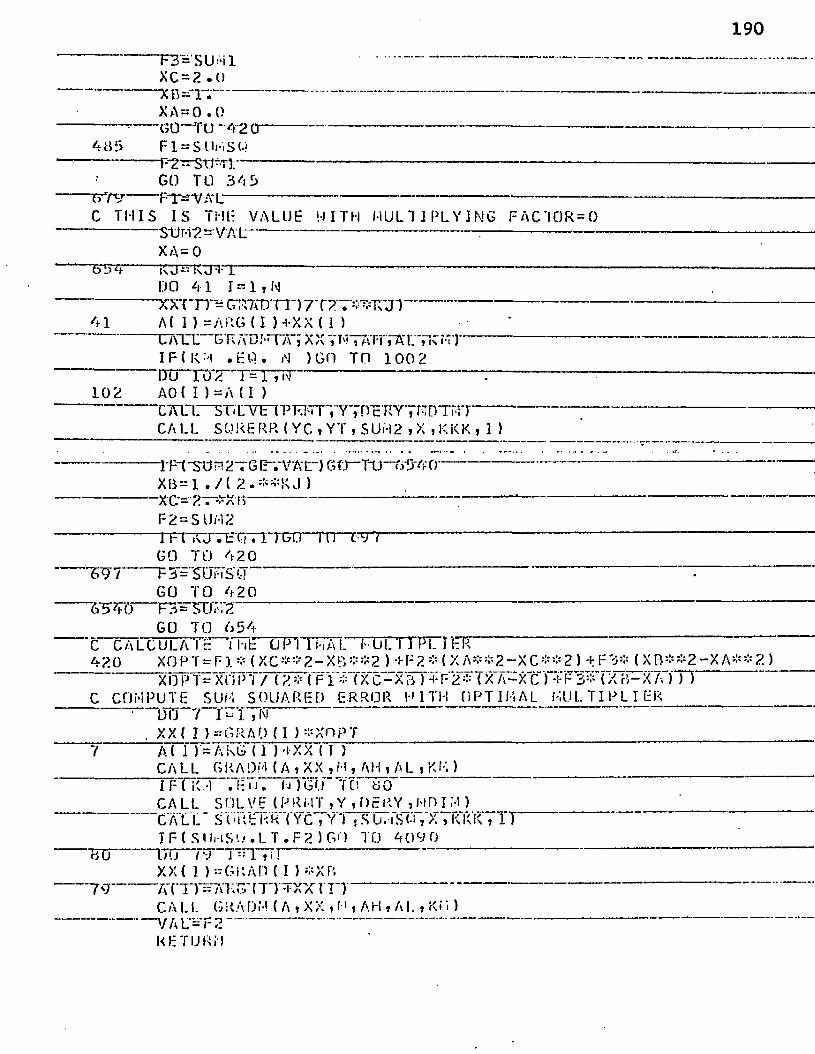
190T 3 = 'S L H 1XC“ 2 . 0

------XA^O .0

“ (;0~T U - 4 2CT4 8 5 F 1 = S U i-iS(.)

—

GO TO 34 3 77TV------FT-*V A* L---------

T H I S I S T ill: VALUE WI TH M U L T I P L Y I N G FAC' IOR- O SUH?~VAL-------------------------------------------------- :--------------------------

X A= 0 ~SJXrt iCTT"T\Tmr

DO 4 1 I ~ 1 , HxxfTr=crR7nrm7T7T-^Ts'jr

41 A l l ) = ARG ( I H-XX ( I )XaTTL C Ri\ DF T A j XX * Tv ) A H jA L I7CM) I F ( K ■-! . E q . i'J ) GO TO 1 0 0 2D n “ rO ‘2 ""T = F T i'J "

1 0 2 AO { I ) =A ( I )X7nrir“5r-l-vftt kt-tt"; TTHcTiYTNDTrr)' CALL S U R E R R ( Y C » Y T , SUM2 ,X , K K K , I )

"TFI-SOn 2 TG ETV’A'L") GtT"T U - t ^ X r X B = 1 . / ( 2 . * * K J )-XC-2V-X [j------------------F 2 = SUM2

-r F l^ u-7t-n , r 1G0 TO T 97GO TO 4 2 0

X T '7 F ?=~S07rs'qGO TO 4 2 0

TY5?rO F3_=STJT72GO TO 0 3 4

'C CALCULAl 'S ’t I-iE U P1 1 i-1A I. F UL I TPTTIFIT 4 2 0 X 0 P T = F 1 * ( X C * - 2 - A i V : :* 2 ) + F 2 * ( X A * * 2 - X C * * 2 ) + F 3 * ( X B * * 2 - X A * - 2 )

T o p T ^ x 'c lP T '/T ^ n T X * T x c“ x'fjT+'F'2 * ,TxTT-XcH-'i13 * ”(x lw x 7 T ) ) )C COMPUTE SUM SOUARED ERROR WI TH OPT IM AL M U L T I P L I E R

DO 7 1 =. XX t I }«(.'

7 A ( 1 )’= A iCALL G1I F ( K.t ,CALL St

G R A D( I ) * XO PT

)H {AiXX,N,AH,AL,KM)V'Hu. u j G o ' T ' c r yo

_0L Vfc* (PRi lT *Y , DcRY , N 0 I M )CALL SFfiE RK i'YC , Y'i • S U, iSM ,'X ‘, KKK , lT “ I F ( SI Ji-iS L*. I. T . F 2 ) GO TO 4 0V 0

"BIT L7u / V i ^ T L , 0x x i i ) "Grad 1 1 ) *xp.

7 ' 7 -------- ATTP=70 7T (T7 7 X X I T ) -CALL GR A0 M { A , XX , F-J_, AFl,_AI. t Kf i )

RETURN

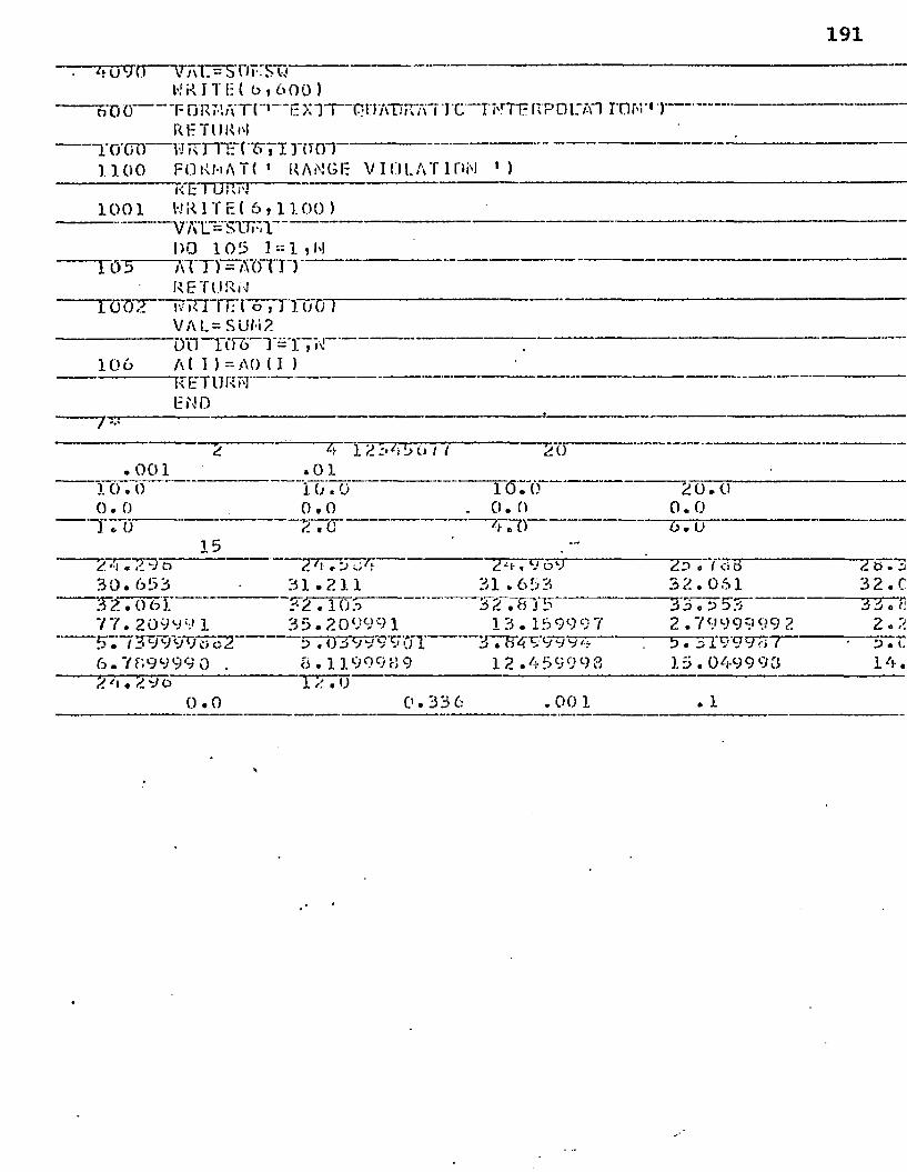
191- . A 'o 'w r— V 7 0> s 'n i-rsT r " “ ......... '

W K I T l : ( 6 , 6 0 0 )“ nOO H jK H n 1 ( 1 i.:X] T C-UADRa i 1C I ITT E KPOl. /-\1 l O n 1 )

RETHUN— IT /o n

1 1 0 0WKJ t t:( to* l l ( i O )F O K N A T f « RANGE V I O L A T I O N ' )Kb 1 URN

1 0 0 1 W R IT r.( 6 , 1 1 0 0 )■■■V/VL=sTrj'r"

0 0 1015 1 « 1 , M--------r 0 y A C ir ^ A o T I" ) ' "

R E T O 0 0---- r 0 -0-r ■ iV T r r n r to T ] io o iV A L = S U f i 2o n ~ i'o 6... .......................... . --

1 0 6 A ( I ) ~ AO ( I )“RE TIJ KM'END

7 -" 2 7T \ 2 11 5 o'

. 0 0 1 . 0 1

1 0 . 0 1 0 . 0 1 0 . 0 2 0 . 0

0 . 0 0 . 0 . 0 . 0 0 . 0

1 . 0 ' 2 . 0 .......... 9 . 0 6 . 0

152 . 6 . 2 0 o 2 A . 5 0 6 2*1 , 9 o9 2 ? • f citi 2 6 .33 0 . 6 5 3 3 1 . 2 1 1 3 1 . 6 5 3 3 2 . 0 6 1 3 2 . C3 2 . 0 61 3 2 . 1 0 3 3 2 . f tJ 3 .................. 3 3 . 3 53> 3 3 . ii7 7 . 2 0 9 v 9 1 3 5 . 2 0 9 9 9 1 13 . 15 9 9 9 7 2 . 7 9 9 9 9 9 9 2 2 . 2

5 . 139999c>o2 3 . 0 3 9 9 9 5 0 1 3 . 6 4 5 9 9 9 6 3 • 5 1 9 S' 9 <i f 3 . t.6 . 7 0 9 9 9 9 0 . b . 1 ]. 9 9 9 0 9 12 . 6 5 9 9 9 3 1 5 . 0 6 9 9 93 1 6 .2 9 . 2 9 o 1 2 . 0

0 . 0 0 . 3 3 6 . 0 0 1 . 1

192

FORTRAN IV Coding of the Minimization Methods not Used in the OMA

As has already been discussed in Chapter V, the following search methods have not been used with the OMA developed in this dissertation.

1. Pattern Search (subroutines PATERN and EXPLOR)2. Fletcher-Powell Method (DFP)3. Fletcher Reeve Method (UPDATE)4. Continued PARTANOf the above, the continued PARTAN was coded as part

of the main program used to derive the OMA. The coding of this particular method is relatively straight forward and, therefore, has not been coded as a subroutine. The other search methods were programmed as separate subroutines and are listed below for possible use in other minimization problems.

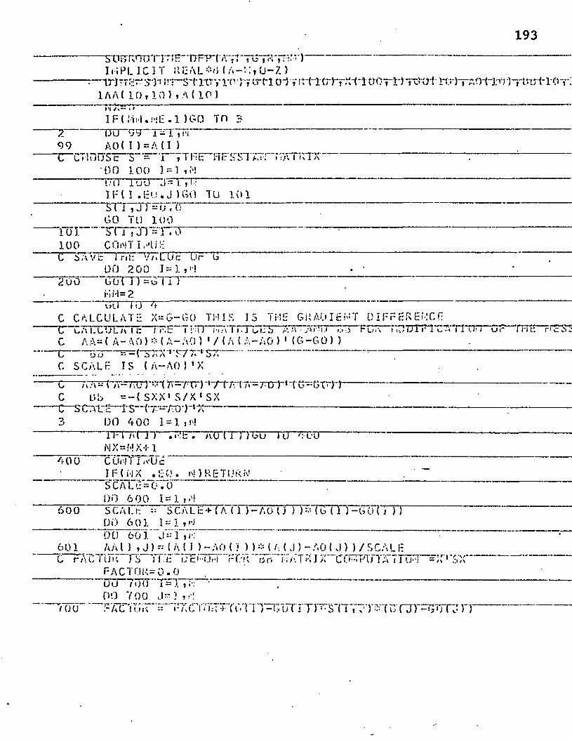
193■StiiT KTTOTrr I IT "PFPT/Y*,'1 *7GTa*iTFr )' 11 i P L IC IT i\ i: AL J ( A - : : t 0 - 1 )

1 a A ( 1 0 , 1 0 ) , M 1 0 )I S A " *•I F { I-ii l . i ' l l : . 1 )G 0 Tn 3

~2-----DU~9?~r=T7n9 9 A0( I ) = / ' , ( ! )

X - CT I 0 D'ST: S~=~_'i 7T ITEXTTF'S’STTATrXATITITT 00 1.00 ].*]. ,Mim rex x='r ,t .:1 1- ( I . I:1.!. J ) GO TU 101

“ s l“ IT J r= ijT oGO TU 100

101 S"(T > Jl ""1 .TT’io o CQt'iT~C Sa vc TrTfl 97riT0"c D r b

00 200 1=1,0 • 1 200 GtTTTl-GTn

i‘!M= 2"uTT TD 'T ........................ ””

C CALCULATE X=G-GO T H I S IS THE Gil AO I EOT 0 ! I: F £R EMC FX C'A'iX'O'L'/i'ri: TDE“ Ti T) ” 7 TFT'CTTS A TrX X X T.T3 F IX i"TTD I rTC X TTO n 0 r Tn c: ruTX C AA= ( A - A O ) * ( A - A O ) ' / ( A t A - A O ) ' ( G - G O ) )

X 57j ( X X a ' T 7 TC'SX— ------------------------------------ 7--------------------------------------------------- --C SCALE IS ( A - A O ) ' X

X r i7 r ^ r /T = 7 x r )^ x ~ n T ) ',7 X r r ( n “ 7Xr)~, 'C'G“ GTn-r C Ob = - { S X X * S / X ' S X x ~ s catts- i s “ ( x ~ ao* )■'a-------------------- — ----------------3 DO A00 1 = 1)!'!

I'F t Al l l — rD F 'T ' AO ( I D X u i lJ~XTX-------MX=MX+1

4 0 0 CUOT I a'UcI F (MX .£0. 0 ) RETUk HS C A L E * 0 . 0 DO 6 00 1 * 1 , . ‘I

6 0 0 SCALE = S C A L E + ( A ( I ) - AO( I ) ) - T b T T I - G O l T T TDO 6 0 1 1 = 1 , 0OCJ 6 0 1 J =! , ! • :

_o 0 1 A /0 1 , J ) * ( A J I )_- AO t j ) ) jM A ( J ) - A 0 ( J ) ) / S C A L I:C rA C T i’JK I S T lX iXEbiTri F f x tir> A / \ T K I 71 cU -O-'Tj TA TTijD =17' SX

F A C T O I D o .OLAJ T o o 1 = 1. ) ;■: ' “ "

n o v o o , i = i , Hi o o ‘ f a c iM 1r * = 'T - A ( r r n i T T 7 'G ' r r i ^ 7 n i T P x ' ( i 7 “ ') ' - T n m ' ^ ' T T j r r

( I i I MO 4 A4;{(! 4 A 4 1; :. / v * I i J S IT'-'O______________ 'j y „

So :) •!•( f ) 07 = ( I ) V i l L L - I 0 0 2 f id

ox ti.l n o t i * fi1'* r ) d i 20=0 X

;: £ Cj t1 * ( 55 ) AXdCi *T ) A4 ( d ) J.M>kl /£ i i-t) Ji>JJL^jii^SJL{J.M ALL'M lLO 0 I L r L * . (U J I LA a 1 tot_) v s-'fi*-Anno ___

( OX ) I -1) (i * ( 1 1 0 0 X ) X 1 ( 0 X ) 0 7 1(0 I S a t ’ I Cl______ ___________. (. ) ff»T/3W .1(0);tr.JHr_ .....t r4: ins4 ■'!4sd34 ov) lui<ixfi -io r 11inyons "

________________C!ii=L M4 n.134

_U- uii£iui-=i.(-i- jiU iaa-----zaz—( i ) >i= ( i jcn cn r

i±L.ljL.U-ZU'd— ClV-------2-CLX------CTIlJd/( I ) aiOV«l-i3l,,:!+ ( I) UV40* ( x - ) “ t I )'J £ 0 2_______________________________________ £-u4 _ a q --------

C I ) 0 V y 0 * ( I ) (J V >i0 r M 3 Mr* = I-! HKd 107.4,..f4.r.]4 £i4K 4 -I4 - G 4 4 4U- n o a d - f M ad---------

»M * 'L = I 1 0 2 fjfl------------------ joao^U3 iiU-------

o * o = m o d 007JiXLL—Q I.....Oft_________

( I ) OV 4 0 * ( '£—) = ( I ) M 001_______ uJAJl=LL GLai— 0 0 ____XCLL.2=u

0X7. n i n n ( x ________ _~(o7 ) onny * t oz ) aioo4 ( o 2 ) v 4 c o 2 ) a v>io noi si-3!•!i a f-/,n«p-7) c:-..Trfii» inn d i ’ii

{ M * * 1 * 0 7 4 0 ) i l l V O d n 3:‘!£ J.fiCi'<jV:nS '________ GO 3woni3>iMf»T i nnv: t r. vi M;=m v; s-w-i r ■■< r *■ on-i :-nyw.~is> w q

( D o * ( r * i ) s - ( i n> = ( i >4 oos LJ_*„L= l._DO_________0*0=(1)4

;>t4T~r no;: np y_2 =!- S — = V! 4 0 1 0 3 A K O I 1 0 3 4 I 0 3 H I G O I d 0 _ _ _ _ _ _ _ _ _ _ _ _ _ _ _ _ _ _ _ _ _ _ _ _ _ _ _ m ^tMr tog on a

( I ) 7 = ( I ) 0V— ;n;ua__aci&_Qa-

( r 41 > *K3 -1 r * n v v * i r 11) s = ( r * i )s o o3- - - - - - - - - - - - - - - - - - - - - - a u a ~ o . a o _ a a ___ _ _

n *1 = 1 0 0 a o a------;ai-4 3 4 1 —M, I j.auM-j-O-a

) 1.373 / ( r 4 1 ) s * ( t n ) o f j - n ) 0 ) * ( ( >i ) o o - ( 4 ) 0 } * ( 4 * 1 ) s + ( r 4 n * 0 = t r * 1 ) « n x o i : j J_.[ x~l-OL-MO-------0 * 1=4 x o i no^o_*XL?U-iii.i-o:ij_ _n * x = r x o i oa

■id.* I “ I. . IJ!1„Q C L

*761

195 ------------ c t t l l ' ;s\“ T':-n,Ycr1 y t v s u t t i t x yicrrcTTT

I P ( SlJi-ij ' . L T . St.l:’i ) til) TO A* p-------------7TTT=77CAT I'T-TrT- SC COl i i ’UTF; SUGARED ERROR~~C7\Tr~ST ■ UV'n'PKnTTYlTTP RYTrtnrr)---

CALL SUREUK (YC » YT‘, SUMM , X , K K K , 1 ) “ IT-1 'STJTTTTVtT. ST 10 ) CTO" T G T ----------------------

6 ii= i-l+ 1 — Am ” cc - m ----------------

GO TO 200- - - - - 3'D7-7'^S1TTTT- - - - - - - - - -200 COOT I OU i:

~1 n-t .•>.!: u )'G0 lu V8 00 111 I - 1 i 0

T X T---nTTTTT en^'iinTJ = 2------- FTHTURTj-------------

9 J= 3 i<.ET“UTT?l

10 DCJ 2 ^ 1 = 1 til' 7 zFv-------«•■( - n = 7vctti i -yi TTir■ ( n ----------------------------C COMPUTE SUGARLO ERROR

--------------- CrArlrt—SiM: V ir(TJf ’Tn f-TY‘T,li?;'L¥-Tt*f?iT‘i-)-CALL SORE HR ( YC , YT , SUGiM , X ,KKK» 1 ) ~rrirSly~ i ■; L T .-J> I in-) 0 0 —1*0—l_i ~ ----------------D O 115 1 = 1 t ’M

T T 'j- - - ft I T ) — A O ( T ) —GO TO 3

TT~~~ S\3Frz$tffi7'*--------I IET U RH'£ j.ipSUIJROUT I U E PATERH ( AL , AM , f 1, V AL , EP S , !< )

--------------- 1 7 T P O X 1 T " R C T T im 7i=Tf7 LF7TY---------------------------------------------------0 I ME US I 0 11 AL ( 1 0 ) , A K ( 1 0 ) , A 0 ( 1 0 ) , X ( 1 0 0 , 1 ) , DELYAt 1 0 )

---------------ro-TuUr! 770771 TY T 1 T rC T m n iT T tT ) 7YC'CTOO ) T O O T O ------COMA*Of I /C i -‘M3 / PR.- ’.T ( 5 ) » Y (5 ) , D E R Y (5 ) , Ml") 1 M , . oDU 1 0 0 1 = 1 t N

T o o a o i j ) = r : r nSUi-i= VAL

*T " = T -------------------------------------------------------------------------J=1TAi:L E XFEE. 7■( A0TTrp'STT”fSTJMTT)" I F ( J •: ‘H • 3 ) GO • T 'l A "77nTtrrr-, rrr.-nT

1 0 0 0 FURi-iATt 1 t* XP L ORA T I Hi I MOT SUCCESSFUL » TRY AGO Yl !-:R .Mini JOG* )

[JO 5 0 I = 1 , MT j ----------77t- r ) ' “ T.n,l “l - )------------------------------------------------------------r—7— :--------------- -----------------~~— :— ;

K= 1 • •

196

Ti b ), *0) 1 = 1 -i- - ■ .............................. ....1 ?.o DELTA* I ) - A t I ) - AO t I )

L “ *-no n o i - 1 jm

l i t ) A 0 ( 1 ) - A < 1 ) GO TO 7

fi no i o i m , i \ 'D E L T A * I ) - D E L T A t I ) * A ( ] ) - A O * I )

1 0 1 A0( ) ) = /. { J j. C i;A Kli PATTERN ROVE

7 LU) 1U b 1 = 1 , i')10 6 At I ) - AO ( I ) + O E L T i \ * I )

9

C COr-i

CALL G ft A DM (A i D c LTA ii'i t A H t AL ,H ) .*~rr( TiTFTTrn'Grr-Tu- :ps--------------PUTS Sl.'i-i Si-'1 ERROR

C rt L L. S L. L V e t lr !T-7T' j Y yrrSTtYTv H I PT)--------CA I. L S 0 RE RR ( Y C , YT , S U ,:r! t X , KK K , 1 ) n~{ s ijMT-rrcTrsnm git T u 13

14- FACT 0 R ~ 0 . 0 T)ti~]:'a''fr-'nn;TTrD E L T A ( I ) = D E LT A ( I ) / 2 . f)

....... n i T P A C T u :\ = r aO 1 U ■< ’l i ) L L it > ( I ) IJ L L 1 A ( I ) I F t F A C T O R . L T . O . l D - 3 ) G f l TG 1 0L= 1GO TG 9

1 0 W i d 1 l: 1 6 j 10 0 1 J1 0 0 1 FOROATt 1 OLD PATTERN OUT S U C C E S S F U L . R E T U R U TG CALL JUG PRG6RA)C S i Ai< i A J.'ul'j PA ) 117 0 0 1 1 3 - 1 = 1 , Nl i b A l l ) = AO I T )

VA L= SUMK „ i - . - ■

* RE TURN.T 1 -'J b Lti-I = s Ut-iri

■00 2 0 0 1 = 1 TJ‘12 0 0 / v 0 1 I ) = A 11 )

GO TO 2

Sl'R R'.Jlj t l ’.Vt" PTSTTTtG i >'-• i !:T* T t S*TTi » 1 C: ii ! i A' i : - m ”

• s i :'y P 7 ^ n ' n :X n r n v - : r r r n i - z n w r m ttx-< w p — T T m - r v n n t o t1 A r I ( 1 0 )

st w ^ f n n W r T S ?r n r 6 r; p c i o o ) , yc 1i o n , k k k » 1Cf Jri.A i j I ! / C 1;! 3 7 P i CVf ( 5 ) iYJ 5 ) ifM: k Y *5 ) i nj. L.____

29DU 29 3 = 1»•'ARC( i ) = A I I )i\'Tt .i.u a T’E"y o oTTo ) = :d Y; rp; CTi;:*.

V I-ACT t . ' i i ) - < 1

197DU '•!) i = 1 j i-i

30 FACTU.; - FACT1 JiUI'R ( I )*G 11 )3 i i - ( DAdS { FAC ti .L;) . 0 1 * 0 . l H - 1 3 ) G u i i j 4

Dll 60 I = l , r |6 0 Kt r j ^ f - D - c r i n ............ .........—...........-

FACT)jR= 0 . 0DU fl'j l ~ i ) M

70 FACTUM “ F A C T U R + l U l ) { 3 )4 110 = ( - 2 ) * ( S DM- tr S I )' / F .'•■C I OR

RX=DAGS ( F A C TU i i )KX = USUF I t !<X ) ...... ....... .I F ( DAiiS ( DO ) . GT . K X ) GO TO 4 0GO 10 4 1

4 0 DO=DO*RX4 l J=.lC COi-lPUT E Y ( 00 ) - F t X + 00 )

' '1 1 DU 10 X ] = I , d XX t I ) =UO*f t ( I )

101 AI J ) = AuG (t )-:-L'0*M ( ) )CALL GRADM<A t X X , 0 , A M j A L i K G )1 F ( !\G « E d . !\' )GU 'i 14

c SOLVE T!-!£ O I F F E0'\' AMO COMPUTE ERi<(JRCALL SL-LVt (PU- . I ,Y ,1,‘ ^KYCALL SMREP.K ( YC j-YT , SU; :00 , aV k KK , 1 )Dd L>00 i = j. »i .

5 0 0 XX.( I ) - A ( I )X Y I 7T) —; \ { X ) 2'Kti X+ L.c Y ( 0 ) =Cc "YD'DTt 0')'=Tjc Y ( DO) = At DO ) 2+BDO+Cc t'l 1 lv li'iUrl j.\ 1c U= Y ( D O ) “ Y { 0 ) - 0 0 YDDTC 0 ) = A ( D O ) I

■ c .'l 1 i'i'l iiUi-i ='-:A77'A = - {'DT7 W ? A " CD 0 ) 2 = - Y 0 0 1 I u) ( DO) <£/2U U= S U;-iDO-SDU- DO -FAC TURi r { U . L t: . 0 . 0 ID 6

1 D1 = ( - 1 ) * ( 0 0 * i j0 ) * F A C TUR/ { 2 * U )b;j 1 u f

o D1 = 2 . 0 -DO7 DU 10 2 I = 1 » i ;

X X X ( I ) = D 1 - D ( I )1 0 2 'AT T T = /T kG { i 7.-RV1 #RTJ' )~... .

CA LL GKA11.'i ( A j XXX j X: f Ai 1 » AL ?KG )j F I KG j l i In

C SHL VF THE D1FF F A ? ' 1!) COMPUTE ERRORCALL SL'L Vo («'r. •. | ,Y ,OoAY , .!u i- )C A L L SO ME KK ( YC , YT t SUnU 1 r X , X.KK , 1 )ITii 6 0 0 1 = 1 7 i-!

'>00 XXX{ I ) = A ( I )i i* ( S* A il.'0 * 1 i S! i • / ’ !->» Sl'riD 1 . o r . ;• U- ■ ) GU I'.i '>I F ( SU.-.DO .GE . S1 1 )G 0 TU 1 0fid ]. O , > I - 1 ) 1 1

t; o .■ ( l ) ( I j

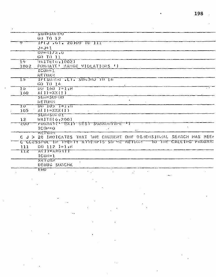
198

'ST3t'i=M7(-‘DO' Gil TO 1?u .....1’FT J ' " . G i . 2 0 " ) GO TCr~l.Tl* ------ --------- ............. .. ‘

J= J + lU O - 0 1 / 2 .0GO TO 3.1

14 ■■JhlTli ( 6 , 100 2 )100?. Ft)lii 1AT( • 2 AOGi: V I O L A T I O N S 1 )

I COiv-3.f iETUKH

1 5 1 F ( SU*-! !.»0 , L ‘l . Sl.fr-. )GU Vl) 3.6 GO TO 14

1 6 0 0 1 6 0 I = 1 ,H1 6 0 A( I ) =o<:< ( I )

SU.-: = S U / D OueTUKO

J. 0 Du 1 06 1 = A j i-J1 05 A( I 1= X X X ( I )

SOri-SUi- 0112 W R I T E ! 6 , 2 0 0 )

1 ZTS'O" FrnVHATt"1 “f : X I ’l T. E S V 'SUiTRCU IT I He: ' ) .................... ..... "1 C !.)!■'= 0t \ C tl) i'i ‘' t

C J > 20 I N D I C A T E S THAT *IHE CUilKlrMT ONE D L 'EUS IC1UAL SEARCH HAS 3EEf0 l.L c b 5 l*U L 11«! I ’. - t rhlY A 1 1 LO-U- I i> SU Wfc lie 1 Uf\N IU li l l: LALL1 Ob K KUurw\.I l l on i i ? 1 = 1 , h1*1 Z At I ) = A K G ( I )

I COH= ].Kc i Ur nDEBUG SU3CHKFK'U

APPENDIX BThis appendix contains details of various computer

runs made in Chapter V toward development of the OMA.

199

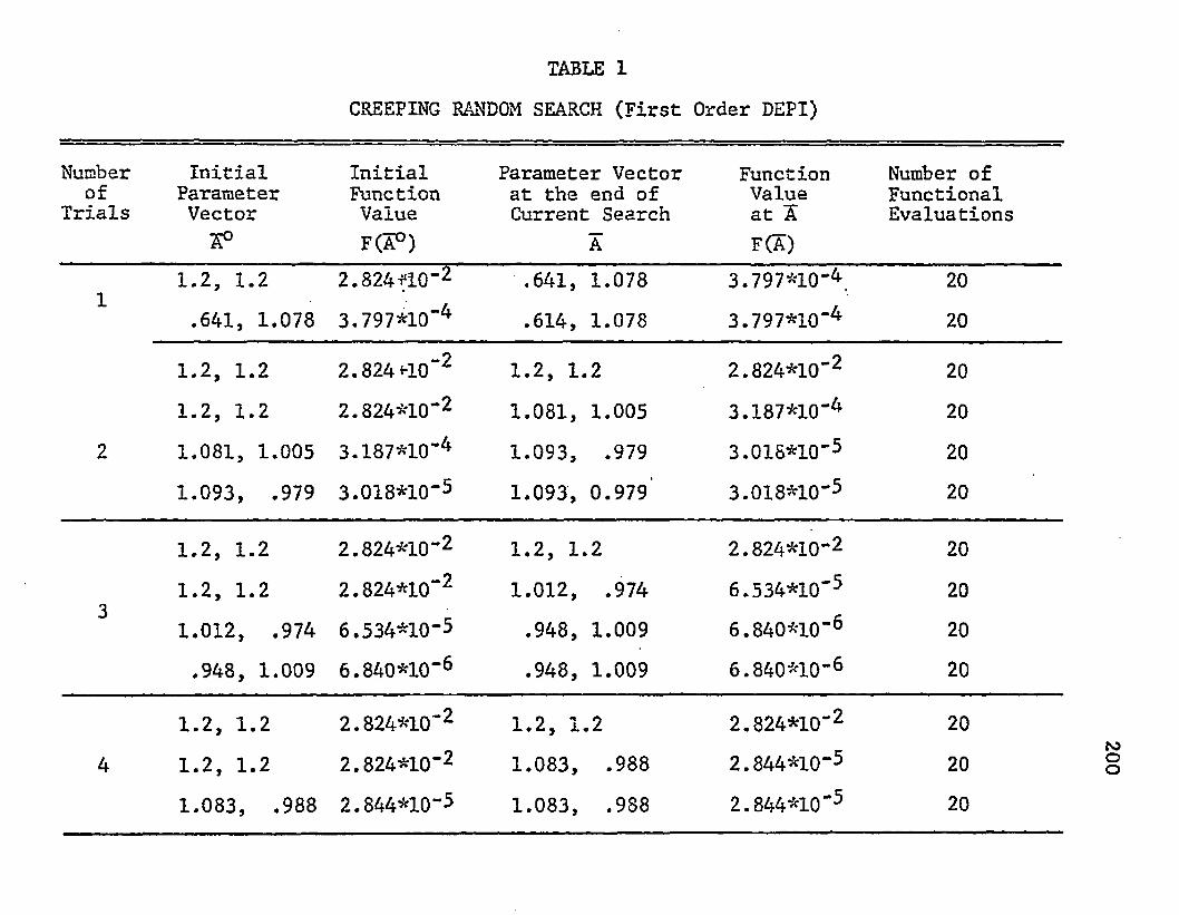
TABLE 1CREEPING RANDOM SEARCH (First Order DEPI)

Numberof

TrialsInitial

ParameterVector£°

InitialFunctionValueF(A°)

Parameter Vector at the end of Current Search

A

Function Value at AF(A)

Number ofFunctionalEvaluations

1 1.2, 1.2 2.824fl0“^ .641, 1.078 3.797*10-^, 20JL

.641, 1.078 3.797*10"4 .614, 1.078 3.797*10"4 20

1.2, 1.2 2.824 HO “2 1.2, 1.2 2.824*10*2 201.2, 1.2 2.824*10*2 1.081, 1.005 3.187*10*4 20

2 1.081, 1.005 3.187*10*4 1.093, .979 3.018*10*5 201.093, .979 3.018*10*5 1.093, 0.979' 3.018*10"5 20

1.2, 1.2 2.824*10“2 1.2, 1.2 2.824*10-2 20

n 1.2, 1.2 2.824*10“2 1.012, .974 6.534*10“"* 20J

1.012, .974 6.534*10-5 .948, 1.009 6.840*10"** 20.948, 1.009 6.840*10“6 .948, 1.009 6.840*10-6 20

1.2, 1.2 2.824*10*2 1.2, 1.2 2.824*10*2 204 1.2, 1.2 2.824*10-2 1.083, .988 2.844*10‘5 20

1.083, .988 2.844*10-5 1.083, .988 2.844*10"5 20

200

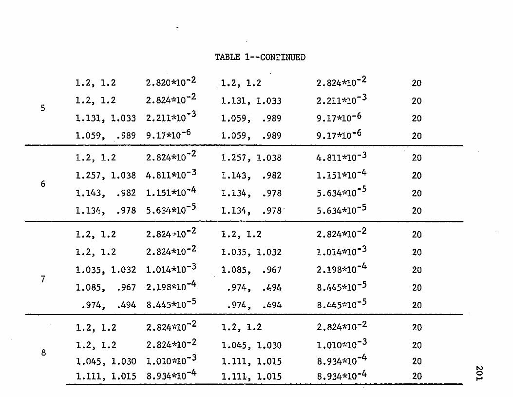
TABLE 1— CONTINUED

1.2, 1.2 2.820 *10"2 1.2, 1.2 2.824*10"2 201.2, 1.2 2.824*10“2 1.131, 1.033 2.211*10”3 2051.131, 1.033 2.211*10'3 1.059, .989 9.17*10"6 201.059, .989 9.17*10"® 1.059, .989 9.17*10"® 20

1.2, 1.2 2.824*10 "*2 1.257, 1.038 4.811*10“3 20

c 1.257, 1.038 4.811*10"3 1.143, .982 1.151*10‘4 20D

1.143, .982 1.151*10"4 1.134, .978 5.634*10 201.134, .978 5.634*10"5 1.134, .978 5.634*10"5 20

1.2, 1.2 2.824+10"2 1.2, 1.2 2.824*10”2 201.2, 1.2 2.824*10”2 1.035, 1.032 1.014*10"3 201.035, 1.032 1.014*10“3 1.085, .967 2.198*10~4 20

/1.085, .967 2.198*10'4 .974, .494 8.445*10"5 20.974, .494 8.445*10"3 .974, .494 8.445*10”3 20

1.2, 1.2 2.824*10"2 1.2, 1.2 2.824*10"2 201.2, 1.2 2.824*10"2 1.045, 1.030 1.010*10-3 2081.045, 1.030 1.010*10”3 1.111, 1.015 8.934*10'4 201.111, 1.015 8.934*10“4 1.111, 1.015 8.934*10"4 20

201

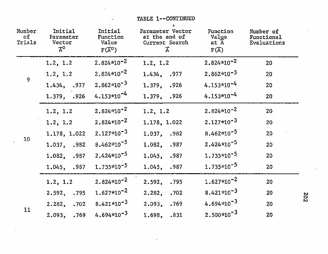
TABLE 1— CONTINUEDNumber

ofTrials

10

11

InitialParameterVector£°

InitialFunctionValueF(A°)

Parameter Vector at the end of Current Search

A

Function Valiie at AF(A)

Number ofFunctionalEvaluations

1.2, 1.2 2.824*10 1.2, 1.2 2.824*10"2 201.2, 1.2 2.824*10“2 1.434, .977 2.862*10"3 201.434., .977 2.862*10"3 1.379, .926 4.153*10"4 201.379, .926 4.153*10“4 1.379, .926 4.153*10"4 20

1.2, 1.2 2.824*10"2 1.2, 1.,2 2.824*10"2 201.2, 1.2 2.824*10"2 1.178, 1.022 2.127*10'3 201.178, 1.022 2.127*10’3 1.037, .982 8.462*10-5 201.037, .982 8.462*10”5 1.082, .987 2.424*10“5 201.082, .987 2.424*10"5 1.045, .987 1.735*10"5 201.045, .987 1.735*10"5 1.045, .987 1.735*10“5 20

1.2, 1.2 2.824*10"2 2.592, .795 1.627*10"2 202.592, .795 1.627*10'2 2.282, .702 8.421*10"3 202.282, .702 8.421*10"3 2.093, .769 4.694*10"3 202.093, .769 4.694*10"3 1.698, .831 2.500*10“3 20

202

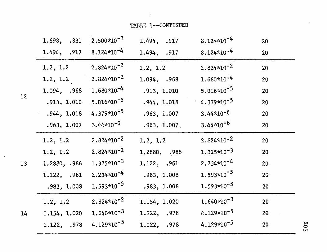
TABLE 1— CONTINUED

1.698, .831 2.500*10“3 1.494, .917 8.124*10”4 201.494, .917 8.124*10‘4 1.494, .917 8.124*10”4 20

1.2, 1.2 2.824*10“2 1.2, 1.2 2.824*10”2 201.2, 1.2 2.824*10“2 1.094, .968 1.680*10“4 201.094, .968 1.680*10"4 .913, 1.010 5.016*10"5 20.913, 1.010 5.016*10"5 .944, 1.018 4.379*10“5 20.944, 1.018 4.379*10"5 .963, 1.007 3.44*10-6 20.963, 1.007 3.44*10"6 .963, 1.007, 3.44*10”6 20

1.2, 1.2 2.824*10"2 1.2, 1.2 2.824*10“2 201.2, 1.2 2.824*10“2 1.2880, .986* t 1.325*10“3 201.2880, .986 1.325*10“3 1.122, .961 2.234*10"4 201.122, .961 2.234*10“4 .983, 1.008 1.593*10"5 20.983, 1.008 1.593*10“5 .983, 1.008 1.593*10"5 20

1.2, 1.2 2.824*10,*2 1.154, 1.020 1.640*10”3 201.154, 1.020 1.640*10”3 1.122, .978 4.129*10”5 201.122, .978 4.129*10”5 1.122, .978 4.129*10’5 20 203

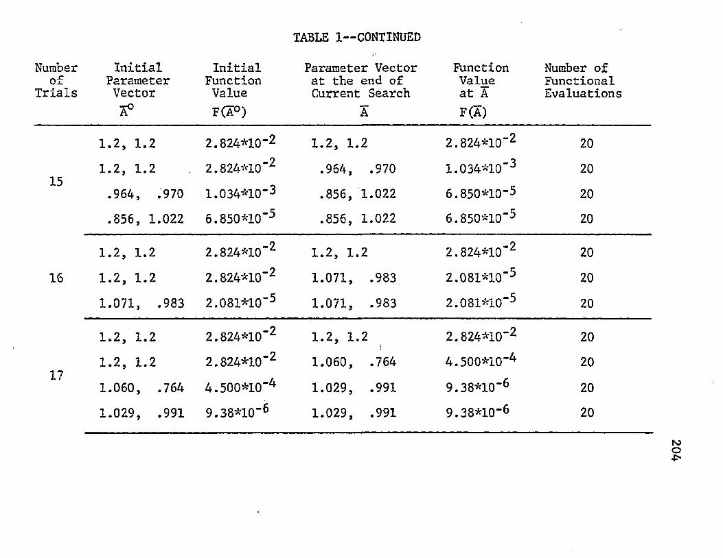
TABLE 1— CONTINUED

Number Initial Initial Parameter Vector Function Number ofof Parameter Function at the end of Value Functional

Trials Vector Value Current Search at A Evaluations£° F(A°) A F(A)

1.2, 1.2 2.824*10-2 1.2, 1.2 2.824*10“2 201.2, 1.2 . 2.824*10”2 .964, .970 1.034*10"3 20.964, .970 1.034*10“3 .856, 1.022 6.850*10-5 20.856, 1.022 6.850*10”5 .856, 1.022 6.850*10"5 20

1.2, 1.2 2.824*10”2 1.2, 1.2 2.824*10’2 2016 1.2, 1.2 2.824*10”2 1.071, .983 2.081*10”5 20

1.071, .983 2.081*10“5 1.071, .983 2.081*10“5 20

1.2, 1.2 2.824*10”2 1.2, 1.2 2.824*10"2 201.2, 1.2 2.824*10”2 1.060, .764 4.500*10“4 20

17 / £1.060, .764 4.500*10 1.029, .991 9.38*10"6 201.029, .991 9.38*10“ 1.029, .991 9.38*10"6 20

204

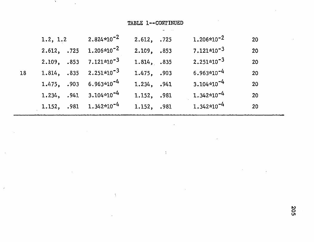
TABLE 1— CONTINUED

1.2, 1.2 2.824*10**2 2.612, .725 1.206*10“2 202.612, .725 1.206*10‘2 2.109, .853 7.121*10"3 202.109, .853 7.121*10‘3 1.814, .835 2.251*10"3 201.814, .835 2.251*10“3 1.475, .903 6.963*10“4 201.475, .903 6.963*10~4 1.234, .941 3.104*10~4 201.234, .941 3.104*10“4 1.152, .981 1.342*10“4 201.152, .981 1.342*10“4 1.152, .981 1.342*10"4 20

205

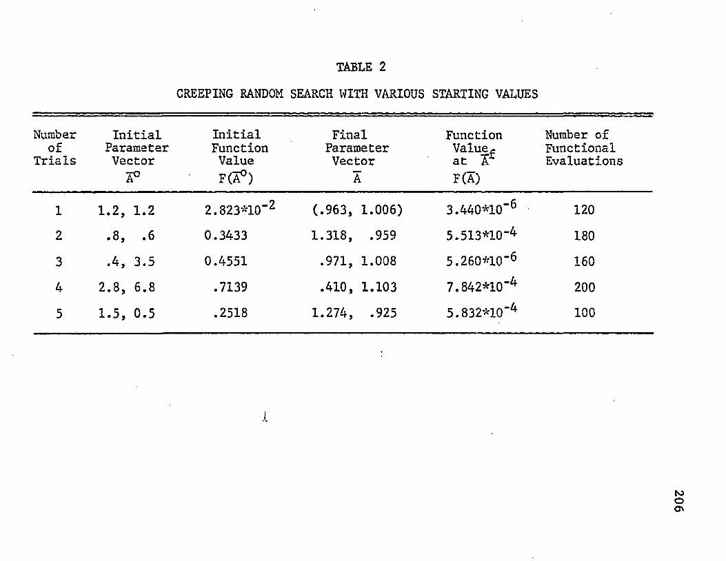
TABLE 2CREEPING RANDOM SEARCH WITH VARIOUS STARTING VALUES

Numberof

TrialsInitial

ParameterVectorA°

InitialFunctionValueF(A°)

FinalParameterVector

A

Function Valuef at AF(A)

Number ofFunctionalEvaluations

1 1.2, 1.2 2.823*10"2 (.963, 1.006) 3.440*10“6 1202 .3, .6 0.3433 1.318, .959 5.513*10“4 1803 .4, 3.5 0.4551 .971, 1.008 5.260*10“6 1604 2.8, 6.8 .7139 .410, 1.103 7.842*10“4 2005 1.5, 0.5 .2518 1.274, .925 5.832*10"4 100

206

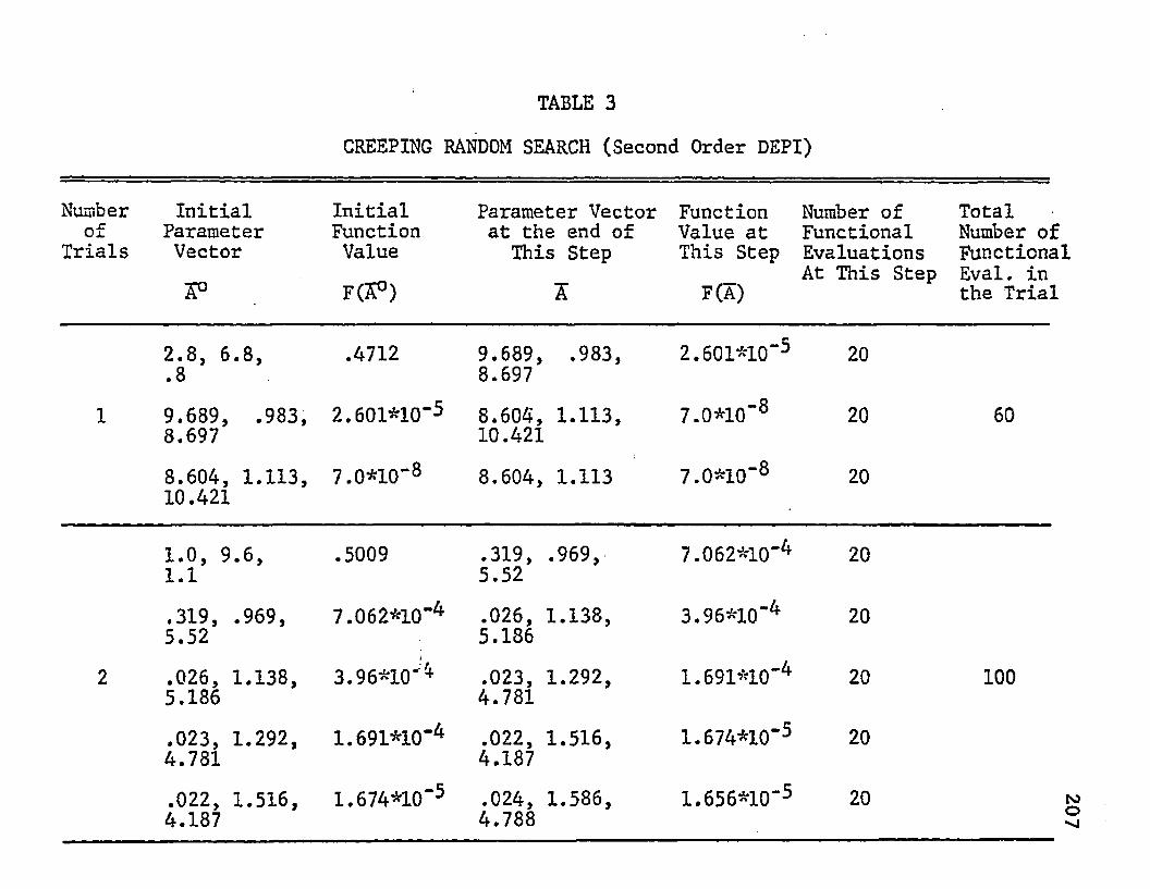
TABLE 3CREEPING RANDOM SEARCH (Second Order DEPI)

Numberof

TrialsInitial

ParameterVectorA°

InitialFunctionValueF(£°)

Parameter Vector at the end of

This StepJ

Function Value at This Step

F(£)

Number of Functional Evaluations At This Step

Total Number of Functional Eval. in the Trial

2.8, 6.8, .8

.4712 9.689, .983, 8.697

2.601*10“** 20

1 9.689, .983, 8.697

2.601*10“5 8.604, 1.113, 10.421

7.0*10"8 20 60

8.604, 1.113, 10.421

7.0*10"® 8.604, 1.113 7.0*10“8 20

1.0, 9.6, 1.1

.5009 .319, .969, 5.52

7.062*10"4 20

.319, .969, 5.52

7.062*10**4 .026, 1.138, 5.186

3.96*10"4 20

2 .026, 1.138, 5.186

3.96*10"'4 .023, 1.292, 4.781

1.691*10“4 20 100

.023, 1.292, 4.781

1.691*10“4 .022, 1.516, 4.187

1.674*10"5 20

.022, 1.516, 4.187

1.674*10"5 .024, 1.586, 4.788

1.656*10-5 20 InC•s

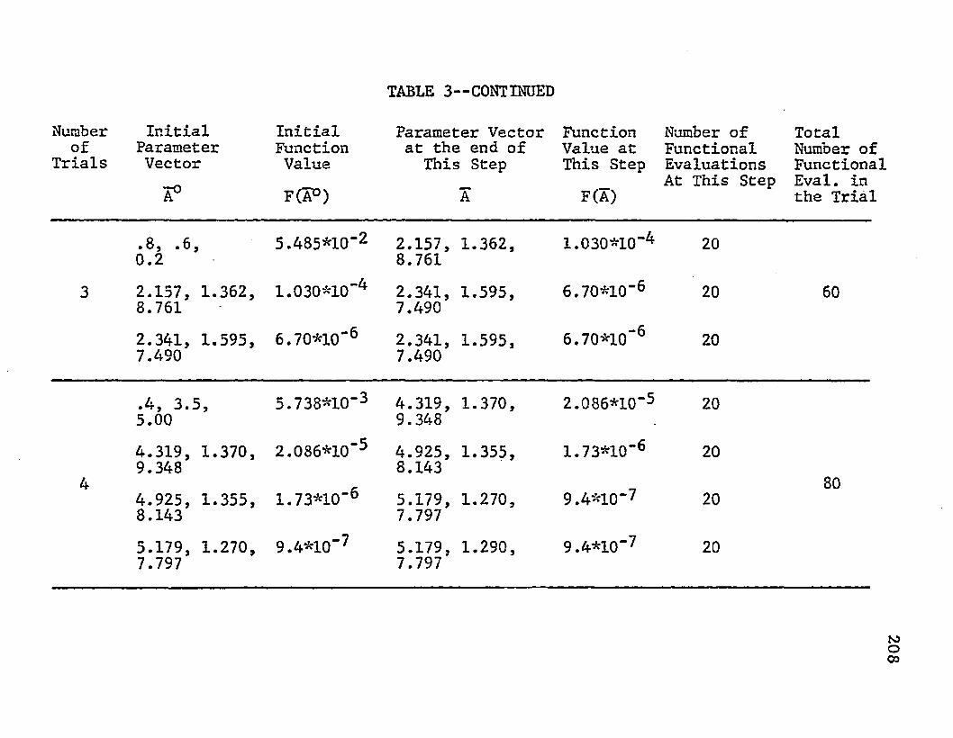
TABLE 3— CONTINUED

Numberof

TrialsInitial

ParameterVector

A0

Initial Parameter Vector Function Number of TotalFunction at the end of Value at Functional Number ofValue This Step This Step Evaluations Functional

— _ At This Step Eval. inF(A°) A F(A) the Trial

.8, .6,0.2

5.485*10'2 2.157,8.761

1.362, 1.030*10“4 20

3 2.157, 1.362, 8.761

1.030*10~4 2.341,7.490

1.595, 6.70*10”6 20 60

2.341, 1.595, 7.490

6.70*10”6 2.341,7.490

1.595, 6.70*10“6 20

.4, 3.5, 5.00

5.738*10'3 4.319,9.348

1.370, 2.086*10”-* 20

44.319, 1.370, 9.3484.925, 1.355, 8.143

2.086*10"5

1.73*10”6

4.925,8.1435.179,7.797

1.355,

1.270,

1.73*10“6

9.4*10”7

20

2080

5.179, 1.270, 7.797

9.4*10"7 5.179,7.797

1.290, 9.4*10”7 20

208

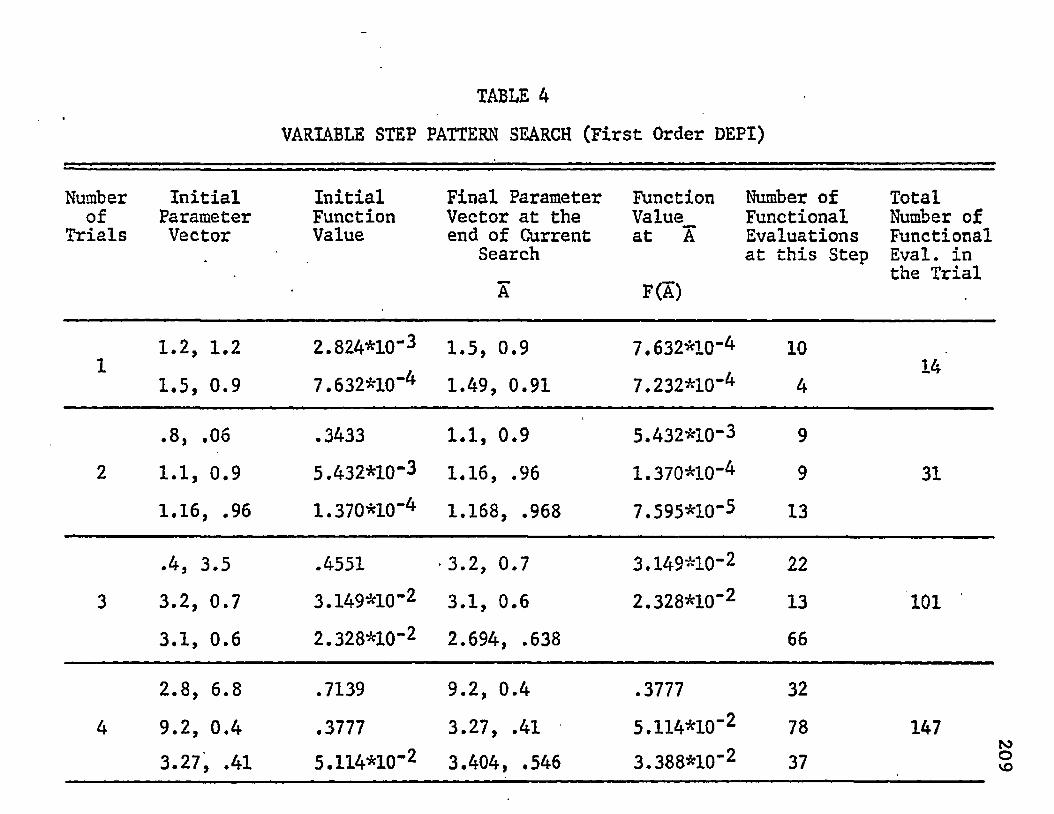
TABLE 4VARIABLE STEP PATTERN SEARCH (First Order DEPI)

Numberof

TrialsInitial

ParameterVector

InitialFunctionValue

Final Parameter Vector at the end of Current

SearchA

Function Value_ at A

F(A)

Number of Functional Evaluations at this Step

Total Number of Functional Eval. in the Trial

11.2, 1.2 1.5, 0.9

2.824*10"3 7.632*10“4

1.5, 0.9 1.49, 0.91

7.632*10“47.232*10“4

10

414

.8, .06 .3433 1.1, 0.9 5.432*10-3 92 1.1, 0.9 5.432*10-3 1.16, .96 1.370*10-4 9 31

1.16, .96 1.370*10“4 1.168, .968 7.595*10-5 13

.4, 3.5 .4551 •3.2, 0.7 3.149*10-2 22

3 3.2, 0.7 3.149*10-2 3.1, 0.6 2.328*10-2 13 101

3.1, 0.6 2.328*10-2 2.694, .638 66

2.8, 6.8 .7139 9.2, 0.4 .3777 324 9.2, 0.4 .3777 3.27, .41 5.114*10-2 78 147

3.27, .41 5.114*10-2 3.404, .546 3.388*10-2 37

209

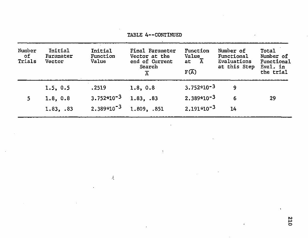
TABLE 4— CONTINUED

Numberof

TrialsInitial

ParameterVector

InitialFunctionValue

Final Parameter Vector at the end of Current

SearchI

Function Value__ at AF(A)

Number of Functional Evaluations at this Step

Total Number of Functional Eval. in the trial

1.5, 0.5 .2519 1.8, 0.8 3.752*10-3 95 1.8, 0.8 3.752*10-3 1.83, .83 2.389*10-3 6 29

1.83, .83 2.389*10"3 1.809, .851 2.191*10“3 14

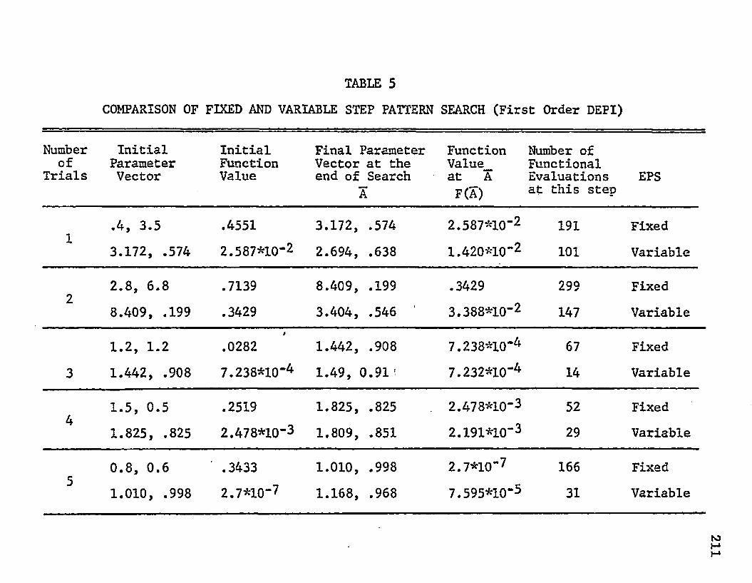
TABLE 5COMPARISON OF FIXED AND VARIABLE STEP PATTERN SEARCH (First Order DEPI)

Numberof

TrialsInitial

ParameterVector

InitialFunctionValue

Final Parameter Vector at the end of Search

A

Function Value__ at AF(A)

Number of Functional Evaluations at this step

EPS

.4, 3.5 .4551 3.172, .574 2.587*10"2 191 Fixedi

3.172, .574 2.587*10-2 2.694, .638 1.420*10"2 101 Variable

2.8, 6.8 .7139 8.409, .199 .3429 299 FixedZ

8.409, .199 .3429 3.404, .546 3.388*10-2 147 Variable

1.2, 1.2*

.0282 1.442, .908 7.238*10*4 67 Fixed3 1.442, .908 7.238*10‘4 1.49, 0.91' 7.232*10“4 14 Variable

1.5, 0.5 .2519 1.825, .825 2.478*10-3 52 Fixed1.825, .825 2.478*10-3 1.809, .851 2.191*10“3 29 Variable

c 0.8, 0.6 .3433 1.010, .998 2.7*10"7 166 Fixed5

1.010, .998 2.7*10-7 1.168, .968 7.595*10“5 31 Variable

211

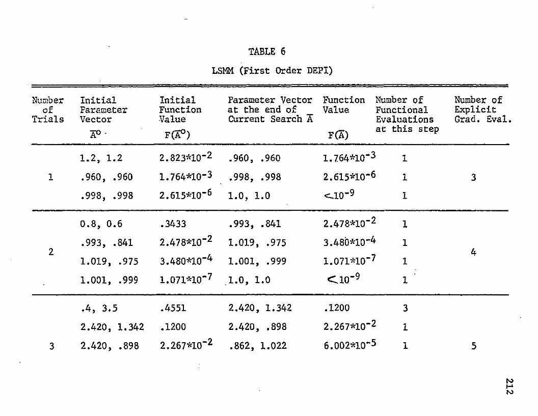
TABLE 6LSMM (First Order DEPI)

Numberof

TrialsInitialParameterVector

-

InitialFunctionValueF(A°)

Parameter Vector at the end of Current Search

Function Number of Value Functional

EvaluationsF(A) at thiS StSp

Number of Explicit Grad, Eval

1.2, 1.2 2.823*I0“2 .960, .960 1.764*10“3 11 .960, .960 1.764*10*3 .998, .998 2.615*10“6 1 3

.998, .998 2.615*10"6 1.0, 1.0 < U 0"9 1

0.8, 0.6 .3433 .993, .841 2.478*10"2 1

2.993, .841 1.019, .975

2.478*10~23.480*10"4

1.019, .975 1.001, .999

3.480*10"4I.071*10“7

11

4

• 1.001, .999 1.071*10“7 .1.0, 1.0 C.10'9 1

.4, 3.5 .4551 2.420, 1.342 .1200 32.420, 1.342 .1200 2.420, .898 2.267*10"2 1

3 2.420, .898 2.267*10’2 .862, 1.022 6.002*10"5 1 5

H

212

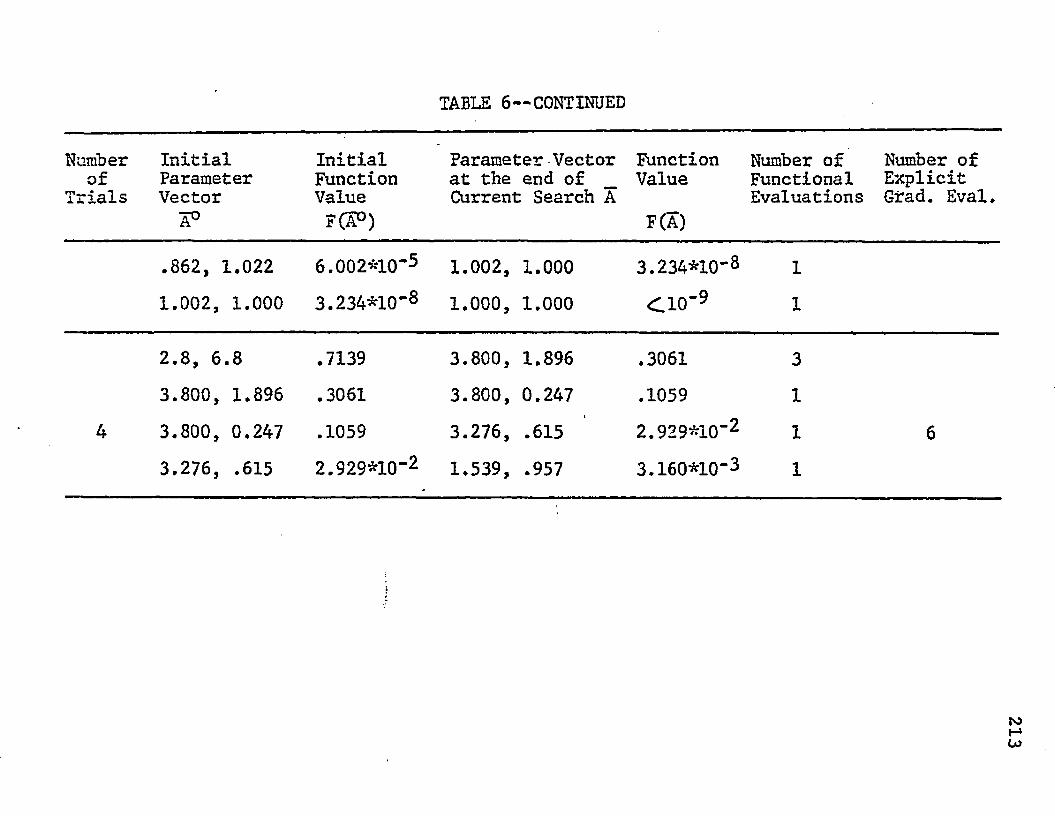
TABLE 6— CONTINUED

Numberof

TrialsInitialParameterVectorA0

InitialFunctionValueF(A°)

Parameter Vector at the end of _ Current Search A

FunctionValue

F(A)

Number ofFunctionalEvaluations

Number of Explicit Grad. Eval.

.862, 1.022 6.002*10~5 1.002, 1.000 3.234*10'8 11.002, 1.000 3.234*10~8 1.000, 1.000 C i 0“9 1

2.8, 6.8 .7139 3.800, 1.896 .3061 33.800, 1.896 .3061 3.800, 0.247 .1059 1

4 3.800, 0.247 .1059 3.276, .615 2.929*i0'2 1 63.276, .615 2.929*10“2 1.539, .957 3.160*10“3 1

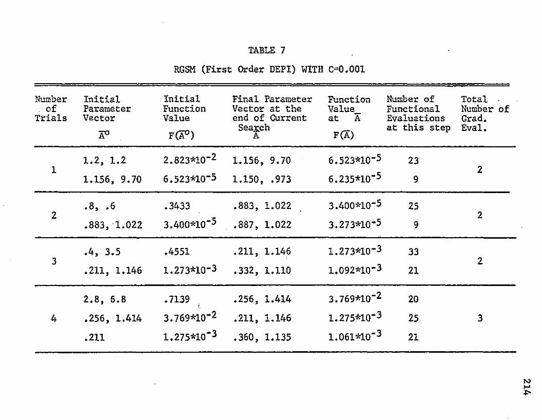
TABLE 7RGSM (First Order DEPI) WITH CO. 001

Numberof

TrialsInitialParameterVector

A0

InitialFunctionValueF(A°)

Final Parameter Vector at the end of Current Search

Function Value__ at AF(A)

Number of Functional Evaluations at this step

Total Number of Grad. Eval.

1.2, 1.2 2.823*10“2 1.156, 9.70 6.523*10“-’ 231 2

1.156, 9.70 6.523*10“5 1.150, .973 6.235*10"** 9

.8, .6 .3433 .883, 1.022 3.400*10-5 252 2

.883, 1.022 3.400*10"5 .887, 1.022 3.273*10*5 9

.4, 3.5 .4551 .211, 1.146 1.273*10-3 333 2

.211, 1.146 1.273*10-3 .332, 1.110 1.092*10-3 21

2.8, 6.8 .7139 f .256, 1.414 3.769*10“2 20

4 .256, 1.414 3.769*10"2 .211, 1.146 1.275*10"3 25 3.211 1.275*10"3 .360, 1.135 1.061*10"3 21

214

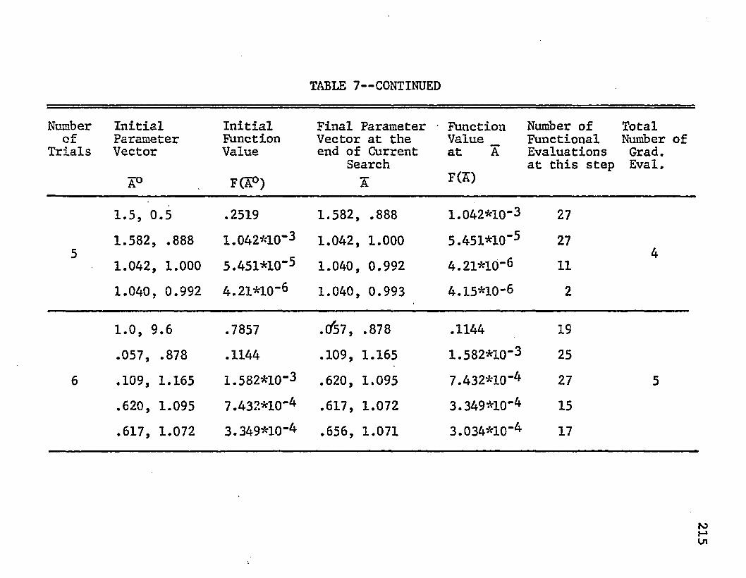
TABLE 7— CONTINUED

Numberof

TrialsInitialParameterVector

A°

InitialFunctionValue

F(S°)

Final Parameter Vector at the end of Current

SearchJ

Function Value __ at AF(£)

Number of Functional Evaluations at this step

Total Number of Grad. Eval.

1.5, 0.5 .2519 1.582, .888 1.042*10“3 271.582, .888 1.042*10“3 1.042, 1.000 5.451*10“-* 27

5 41.042, 1.000 5.451*10“5 1.040, 0.992 4.21*10“6 111.040, 0.992 4.21*10“6 1.040, 0.993 4.15*10-6 2

1.0, 9.6 .7857 .Cf57, .878 .1144 19.057, .878 .1144 .109, 1.165 1.582*10“3 25

6 .109, 1.165 1.582*10"3 .620, 1.095 7.432*10“4 27 5.620, 1.095 7.432*10-4 .617, 1.072 3.349*10“4 15.617, 1.072 3.349*10-4 .656, 1.071 3.034*10“4 17

215

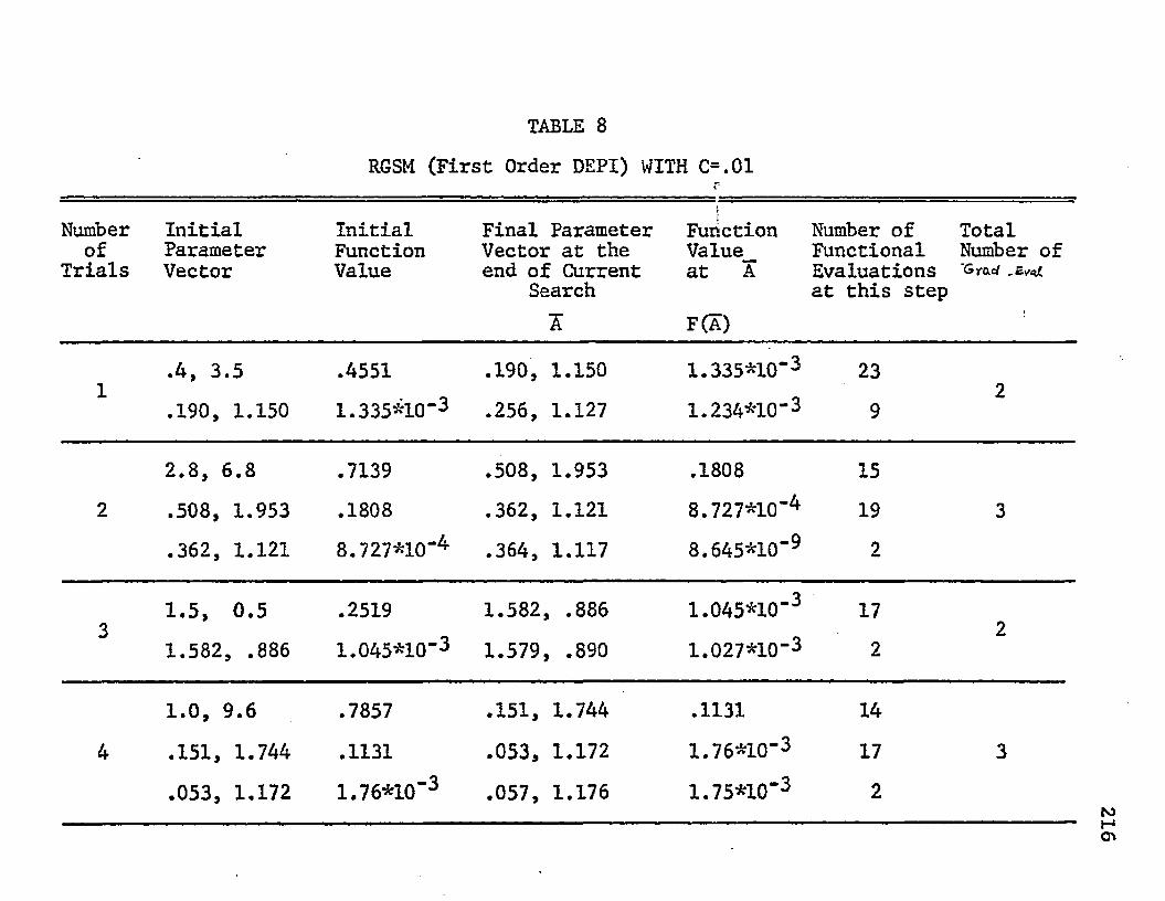
TABLE 8RGSM (First Order DEPI) WITH C=.01

Numberof

TrialsInitialParameterVector

InitialFunctionValue

Final Parameter Vector at the end of Current

SearchX

fFunction Value__ at A

F(A)

Number of Functional Evaluations at this step

Total Number of

.4, 3.5 .4551 .190, 1.150 1.335*10"3 231 2

.190, 1.150 1.335*10"3 .256, 1.127 1.234*10“3 9

2.8, 6.8 .7139 .508, 1.953 .1808 152 .508, 1.953 .1808 .362, 1.121 8.727*10"4 19 3

.362, 1.121 8.727*10"4 .364, 1.117 8.645*10"9 2

1.5, 0.5 .2519 1.582, .886 1.045*10"3 173 2

1.582, .886 1.045*10"3 1.579, .890 1.027*10"3 2

1.0, 9.6 .7857 .151, 1.744 .1131 144 .151, 1.744 .1131 .053, 1.172 1.76*10"3 17 3

.053, 1.172 1.76*10“3 .057, 1.176 1.75*10“3 2 216

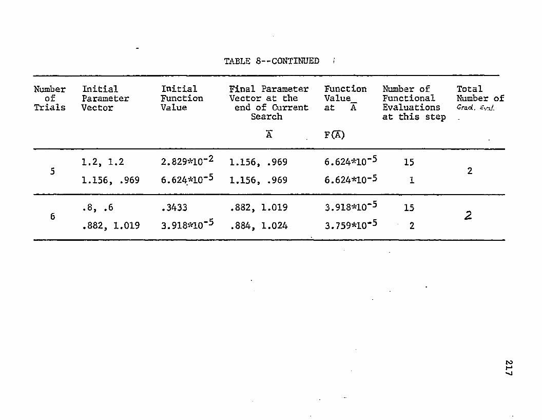
TABLE 8— CONTINUED i

Number Initial Initial Final Parameter Function Number of Totalr \ c 0i* Parameter Function Vector at the Value Functional Number of

Trials Vector Value end of Current at A Evaluations Grad.Search at this step -

X F(X)-

1.2, 1.2 2.829*10“2 1.156, .969 6.624*10“-* 15O 21.156, .969 6.624*10“** 1.156, .969 6.624*10-5 1

.8, .6 .3433 .882, 1.019 3.918*10"5 156 2

.882, 1.019 3.918*10”-* .884, 1.024 3.759*10*5 2

217

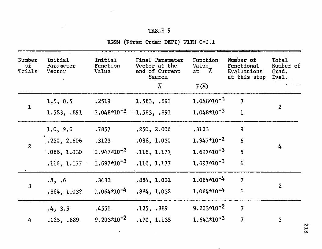
TABLE 9RGSM (First Order DEPI) WITH C=0.1

Numberof

TrialsInitialParameterVector

InitialFunctionValue

Final Parameter Vector at the end of Current

SearchA

Function Value__ at A

F(A)

Number of Functional Evaluations at this step

Total Number of Grad. Eval.

11.5, 0.5 1.583, .891

.25191.048*10-3

1.583, .8911.583, .891

1.048*10"31.048*10"3

71

2

1.0, 9.6 .7857 .250, 2.606 .3123 9

2’ .250, 2.606 .088, 1.030

.31231.947*10"2

.088, 1.030

.116, 1.1771.947*10”2 1.697*10"3

6

54

.116, 1.177 1.697*10"3 .116, 1.177 1.697*10‘3 1

3.8, .6 .884, 1.032

.34331.064*10“4

.884, 1.032

.884, 1.0321.064*10"4 1.064*10”4 1

2

.4, 3.5 .4551 .125, .889 9.203*10”2 74 .125, .889 9.203*10“2 .170, 1.135 1.641*10-3 7 3 218

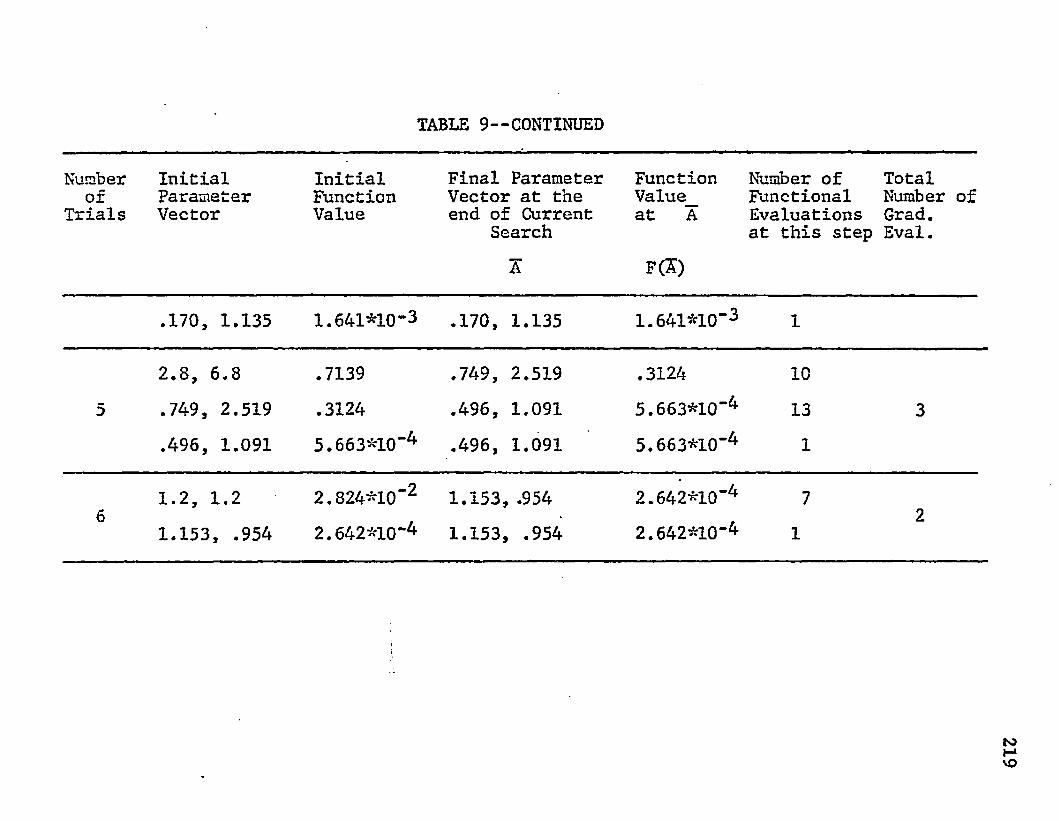
TABLE 9— CONTINUED

Numberof

TrialsInitialParameterVector

InitialFunctionValue

Final Parameter Vector at the end of Current

SearchA

Function Value_ at A

F ®

Number of Functional Evaluations at this step

Total Number of Grad. Eval.

.170, 1.135 1.641*10-3 .170, 1.135 1.641*10~3 1

2.8, 6.8 .7139 .749, 2.519 .3124 105 .749, 2.519 .3124 .496, 1.091 5.663*10"4 13 3

.496, 1.091 5.663*10"4 .496, 1.091 5.663*10*4 1

1.2, 1.2 2.824*10"2 1.153, .954 2.642*10’4 76 t 2

1.153, .954 2.642*10“4 1.153, .954 2.642*10"4 1

219

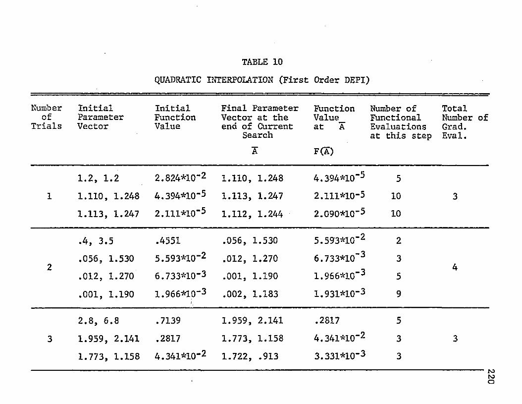
TABLE 10QUADRATIC INTERPOLATION (First Order DEPI)

Numberof

TrialsInitialParameterVector

InitialFunctionValue

Final Parameter Vector at the end of Current

SearchJ

Function Value_ at A

F (K)

Number of Functional Evaluations at this step

Total Number of Grad. Eval.

1.2, 1.2 2.824*10 1.110, 1.248 4.394*10""* 51 1.110, 1.248 4.394*10-5 1.113, 1.247 2.111*10-5 10 3

1.113, 1.247 2.111*10"5 1.112, 1.244 2.090*10-5 10

.4, 3.5 .4551 .056, 1.530 5.593*10"2 2

.056, 1.530 5.593*10-2 .012, 1.270 6.733*10”3 32 4

.012, 1.270 6.733*10-3 .001, 1.190 1.966*10“J 5

.001, 1.190 1.966*10-3 .002, 1.183 1.931*10-3 9

2.8, 6.8 .7139 1.959, 2.141 .2817 53 1.959, 2.141 .2817 1.773, 1.158 4.341*10"2 3 3

1.773, 1.158 4.341*10-2 1.722, .913 3.331*10-3 3

220

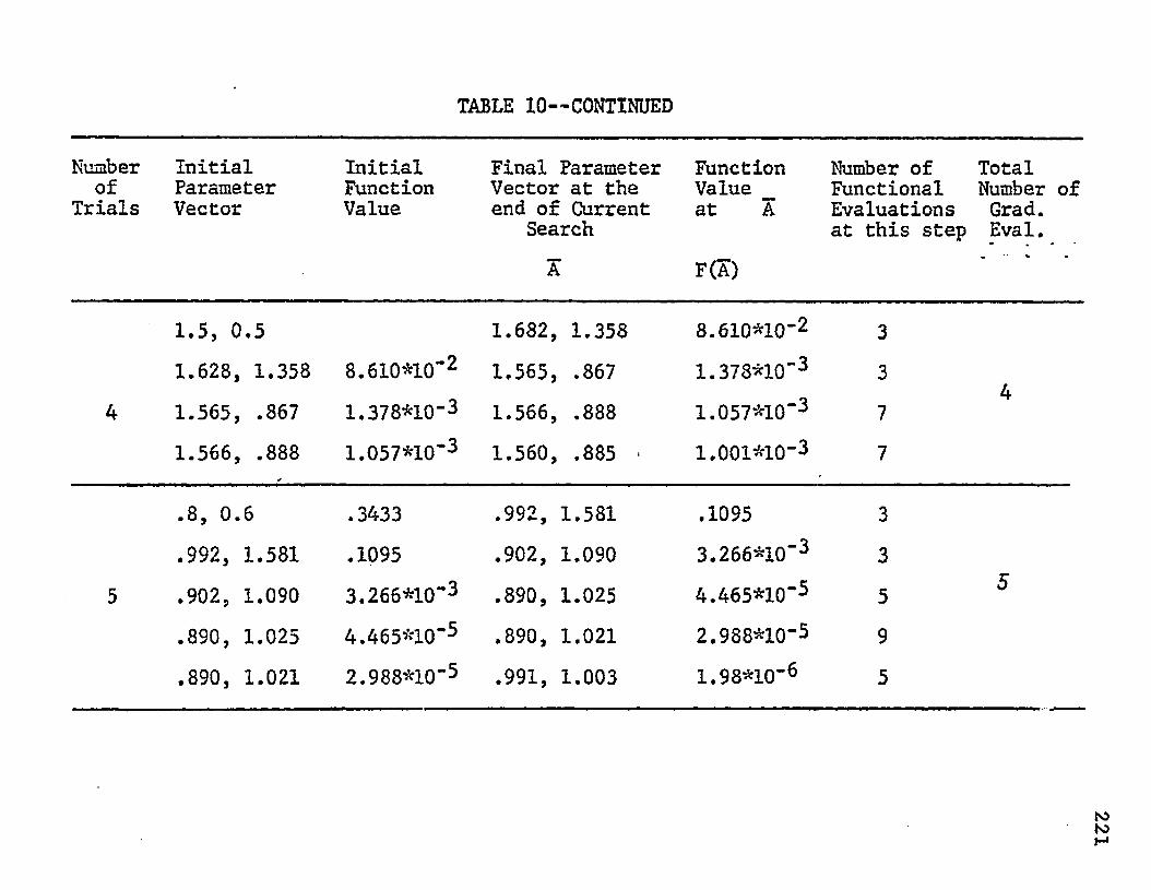
TABLE 10— CONTINUED

Numberof

TrialsInitialParameterVector

InitialFunctionValue

Final Parameter Vector at the end of Current

SearchA

Function Value _ at A

F(A)

Number of Functional Evaluations at this step

Total Number of Grad. Eval.

1.5, 0.5 1.682, 1.358 8.610*10*2 31.628, 1.358 8.610*10*2 1.565, .867 1.378*10*3 3

44 1.565, .867 1.378*10*3 1.566, .888 1.057*10*3 7

1.566, .888 1.057*10“^ 1.560, .885 • 1.001*10*3 7

.8, 0.6 .3433 .992, 1.581 .1095 3

.992, 1.581 .1095 .902, 1.090 3.266*10*3 35 .902, 1.090 3.266*10"3 .890, 1.025 4.465*10*3 5 5

.890, 1.025 4.465*10*3 .890, 1.021 2.988*10*5 9

.890, 1.021 2.988*10“5 .991, 1.003 1.98*10*3 5

221

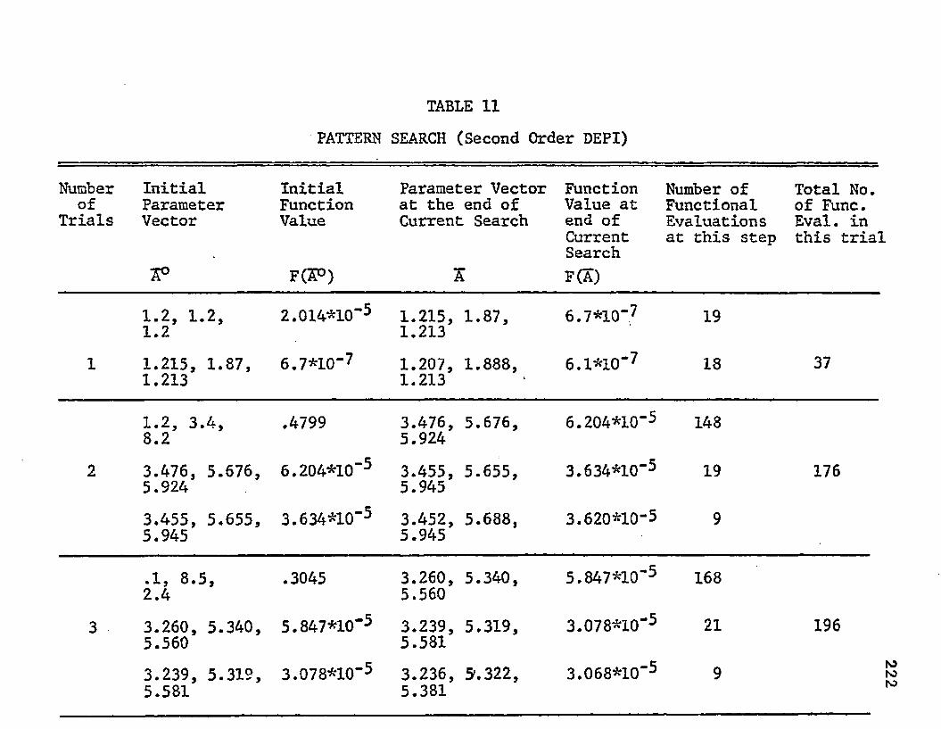
TABLE IXPATTERN SEARCH (Second Order DEPI)

Numberof

TrialsInitialParameterVector

InitialFunctionValue

Parameter Vector at the end of Current Search

Function Value at end of Current Search

Number of Functional Evaluations at this step

Total No. of Func. Eval. in this trial

F(£°) 5 F(A)

1.2, 1.2, 1.2

2.014*10“5 1.215, 1.87, 1.213

6.7*10"7 19

1 1.215, 1.87, 1.213

6.7*10"7 1.207, 1.888, 1.213

6.1*10"7 18 37

1.2, 3.4, 8.2

.4799 3.476, 5.676, 5.924

6.204*10"-* 148

2 3.476, 5.676, 5.924

6.204*10~5 3.455, 5.655, 5.945

3.634*10"5 19 176

3.455, 5.655, 5.945

3.634*10“5 3.452, 5.688, 5.945

3.620*10-5 9

.1, 8.5, 2.4

.3045 3.260, 5.340, 5.560

5.847*10"5 168

3 3.260, 5.340, 5.560

5.847*10“-* 3.239, 5.319, 5.581

3.078*10“** 21 196

3.239, 5.319, 5.581

3.078*10"-* 3.236, S'.322, 5.381

3.068*10“5 9 ii

222

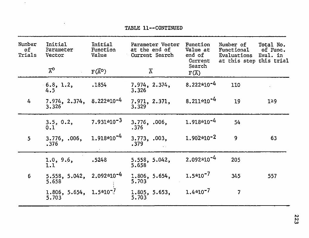
TABLE 11— CONTINUED

Numberof

TrialsInitialParameterVector

A°

InitialFunctionValue

F(A°)

Parameter Vector at the end of Current Search

A

Function Value at end of Current SearchF(£)

Number of Functional Evaluations at this step

Total No.of Func. Eval. in this trial

6.8, 1.2, 4.5

.1854 7.974, 2.374, 3.326

8.222*10*4 110

4 7.974, 2.374, 3,326

8.222*10*4 7.971, 2.371, 3.329

8.211*10*4 19 I29

3.5, 0.2, 0.1

7.931*10“3 3.776, .006, .376

1.918*10"4 54

5 3.776, .006, .376

1.918*10"4 3.773, .003, .379

1.902*10*2 9 63

1.0, 9.6, 1.1

.5248 5.558, 5.042, 5.658

2.092*10~4 205

6 5.558, 5.042, 5.658

2.092*10“4i

1.806, 5.654, 5.703

1.5*10"7 345 557

1.806, 5.654, 5.703

1.5*10"? 1.805, 5.653, 5.703

1.4*10"7 7

223

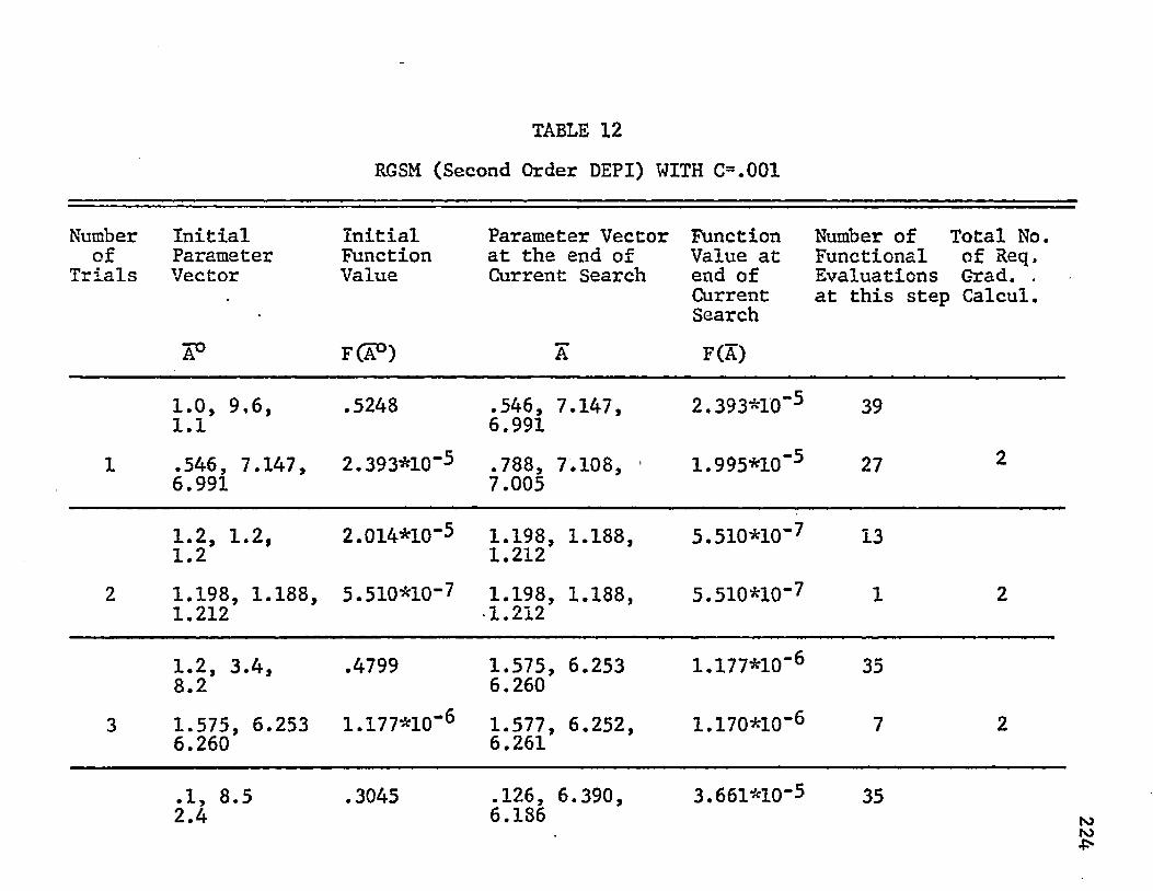
TABLE 12RGSM (Second Order DEPI) WITH C=.001

Numberof

TrialsInitialParameterVector

InitialFunctionValue

Parameter Vector at the end of Current Search

Function Value at end of Current Search

Number of Functional Evaluations at this step

Total No. of Req, Grad. . Calcul.

A° F(A°) A F(A)

1.0, 9,6,1.1

.5248 .546, 7.147, 6.991

2.393*I0~5 39

1 .546, 7.147, 6.991

2.393*10~5 .788, 7.108, 7.005

1.995*10”5 27 2

1.2, 1.2, 1.2

2.014*10“5 1.198, 1.188, 1.212

5.510*10“7 13

2 1.198, 1.188, 1.212

5.510*10-7 1.198, 1.188, •1.212 5.510*10-7 1 2

1.2, 3.4,8.2

.4799 1.575, 6.253 6.260

1.177*10“6 35

3 1.575, 6.253 6.260

1.177*10"6 1.577, 6.252, 6.2611.170*10“6 7 2

.1, 8.5 2.4

.3045 .126, 6.390, 6.186

3.661*10-5 35 224

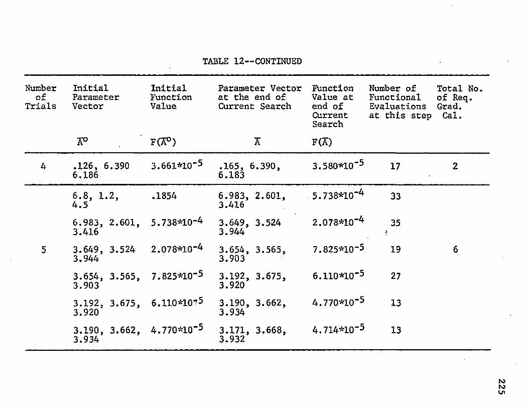
TABLE 12— CONTINUED

Numberof

TrialsInitialParameterVector

InitialFunctionValue

Parameter Vector at the end of Current Search

Function Value at end of Current Search

Number of Functional Evaluations at this step

Total No. of Req. Grad.Cal.

F(5°) H F(S)

4 .126, 6.390 6.186

3.661*10"5 .165, 6.390, 6.183

3.580*10"5 17 2

6.8, 1.2, 4.5

.1854 6.983, 2.601, 3.416

5.738*10"4 33

6.983, 2.601, 3.416

5.738*10-4 3.649, 3.524 3.944

2.078*10"4 35J

5 3.649, 3.524 3.944

2.078*10-4 3.654, 3.565, 3.903

7.825*10-5 19 6

3.654, 3.565, 3.903

7.825*10-5 3.192, 3.675, 3.920

6.110*10'5 27

3.192, 3.675, 3.920

6.110*10* 5 3.190, 3.662, 3.934

4.770*10”-* 13

3.190, 3.662, 3.934

4.770*10"-* 3.171, 3.668, 3.9324.714*10"-* 13

225

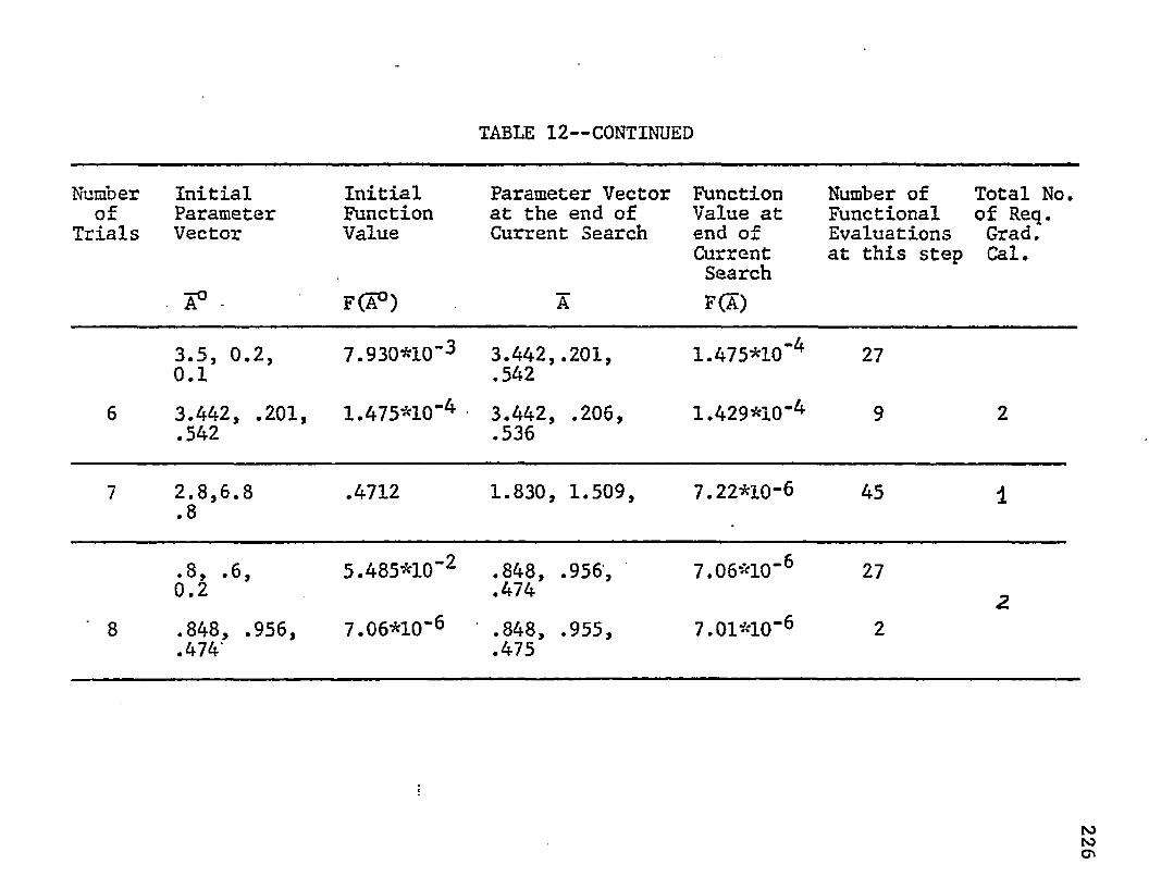
TABLE 12— CONTINUED

Numberof

TrialsInitialParameterVector

A° -

InitialFunctionValue

F(A°)

Parameter Vector at the end of Current Search

A

Function Value at end of Currant SearchF(A)

Number of Functional Evaluations at this step

Total No. of Req. Grad. Cal.

3.5, 0.2, 0.1

7.930*10”3 3.442,.201, .542

1.475*10"4 27

6 3.442, .201, .542

1.475*10"4 3.442, .206, .536

1.429*10"4 9 2

7 2.8,6.8 .8

.4712 1.830, 1.509, 7.22*10-6 45 1

.8, .6,0.2

5.485*10"2 .848, .956, .474

7.06*10"6 272

' 8 .848, .956, .474-

7.06*10"6 .848, .955, .475

7.01*10“6 2

226

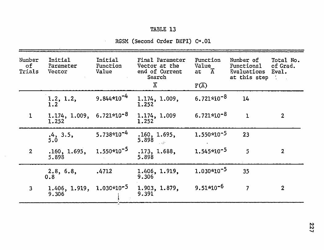
TABLE 13RGSM (Second Order DEPI) 0.01

Numberof

TrialsInitialParameterVector

InitialFunctionValue

Final Parameter Vector at the end of Current

SearchA

Function Value__ at A

F(A)

Number of Functional Evaluations at this step

Total No. of Grad. Eval.

1.2, 1.2, 1.2

9,844*10"4 1.174, 1.009, 1.252

6.721*10"8 14

1 1.174, 1.009, 1.252

6.721*10-8 1.174, 1.009 1.252

6.721*10-8 1 2

.4, 3.5, 5.0

5.738*10“4 .160, 1.695, 5.898

1.550*10-5 23

2 .160, 1.695, 5.898

1.550*10“** .173, 1.688, 5.898

1.545*10-5 5 2

2.8, 6.8, 0.8

.4712 1.406, 1.919, 9.306

1.030*10-5 35

3 1.406, 1.919, 9.306

1.030*10-5!\

1.903, 1.879, 9.391

9.51*10“6 7 2

227

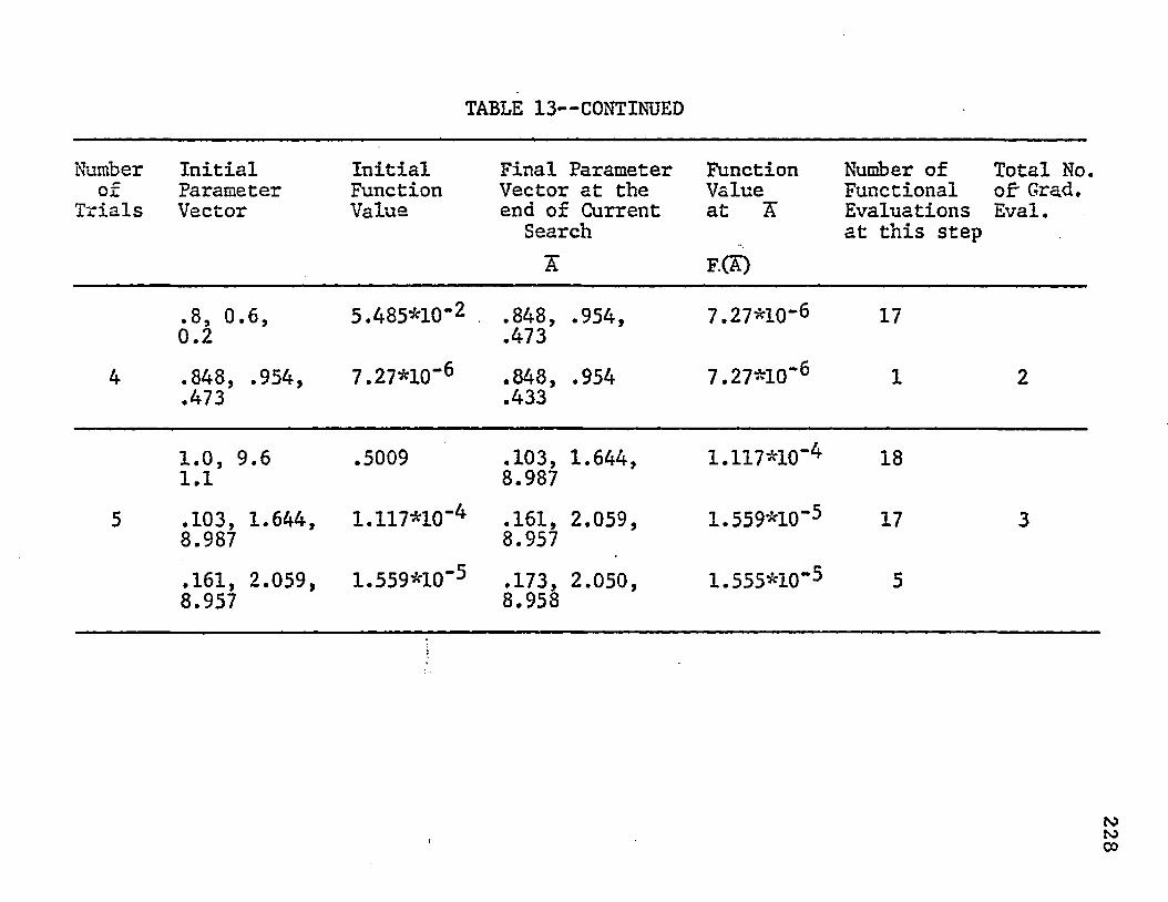
TABLE 13— CONTINUED

Numberof

TrialsInitialParameterVector

InitialFunctionValue

Final Parameter Vector at the end of Current

SearchE

FunctionValueat

fm

Number of Functional Evaluations at this step

Total No. of Grad. Eval.

.8, 0 .6, 0.2

5.485*10"2 .848, .954, .473

7.27*10-6 17

4 .848, .954, .473

7.27*10“® .848, .954 .433

7.27*10"6 1 2

1.0, 9.6 1.1

.5009 .103, 1.644, 8.987

1.117*10"4 18

5 .103, 1.644, 8.987

1.117*10"4 .161, 2.059, 8.957

1.559*10"5 17 3

.161, 2.059, 8.957

1.559*10"-* .173, 2.050, 8.958

1.555*10"5 5

228

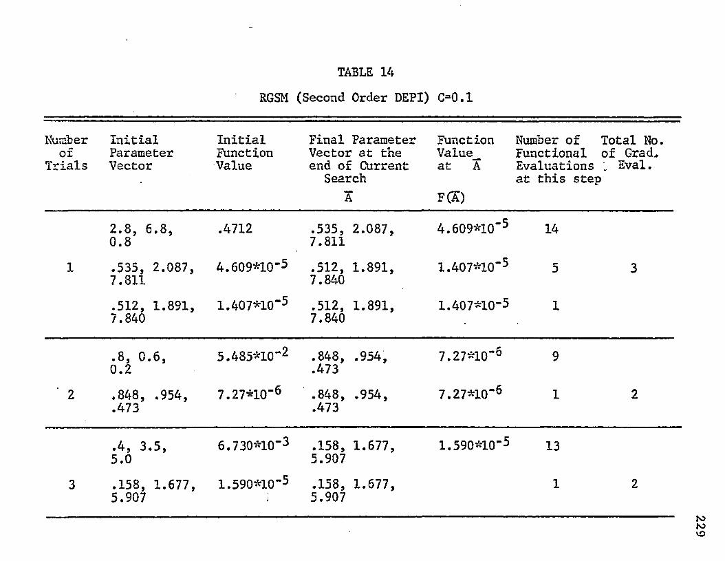
TABLE 14RGSM (Second Order DEPI) C=0.1

Numberof

TrialsInitialParameterVector

InitialFunctionValue

Final Parameter Vector at the end of Current

SearchA

Function Value__ at A

FGO

Number of Total No. Functional of Grad., Evaluations Eval. at this step

2.8, 6.8,0.8

.4712 .535,7.811

2.087, 4.609*10"5 14

1 .535, 2.087, 7.811

4.609*10"5 .512,7.840

1.891, 1.407*10"5 5 3

.512, 1.891, 7.840

1.407*10“5 .512,7.840

1.891, 1.407*10-5 1

.8, 0.6, 0.2

5.485*10"2 .848,.473

.954, 7.27*10"6 9

2 .848, .954, .473

7.27*10“6 .848,.473

.954, 7.27*10"® 1 2

.4, 3.5, 5.0

6.730*10~3 .158,5.907

1.677, 1.590*10"® 13

3 .158, 1.677, 5.907

1.590*10"5 .158,5.907

1.677, 1 2

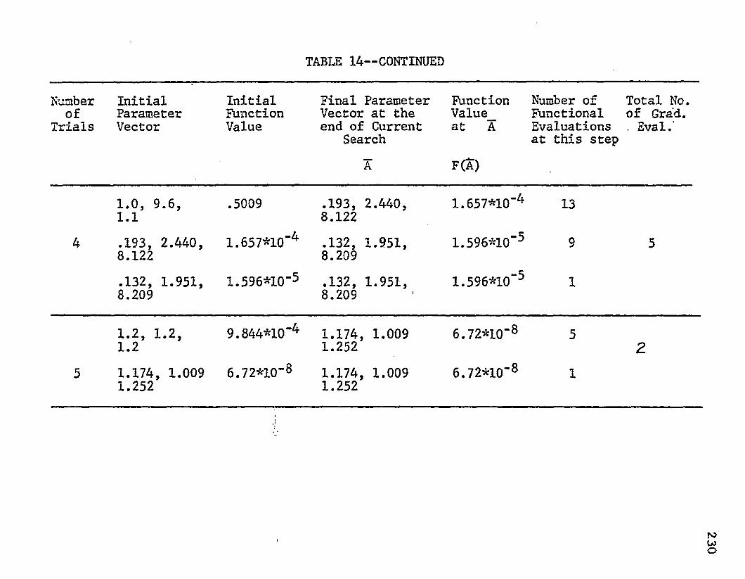
TABLE 14— CONTINUED

Numberof

TrialsInitialParameterVector

InitialFunctionValue

Final Parameter Vector at the end of Current

SearchA

Function Value_ at A

F(A)

Number of Functional Evaluations at this step

Total No. of Grad., Eval.

1.0, 9.6, 1.1

.5009 .193, 2.440, 8.122

1.657*10”4 13

4 .193, 2.440, 8.122

1.657*10“4 .132, 1.951, 8.209

1.596*10”5 9 5

.132, 1.951, 8,209

1.596*10"5 .132, 1.951, 8.209

1.596*10**"* 1

1.2, 1.2, 1.2

9.844*10"4 1.174, 1.009 1.252

6.72*10"8 52

5 1.174, 1.009 1.252

6.72*10"^ 1.174, 1.009 1.252

6.72*10”8 1

230

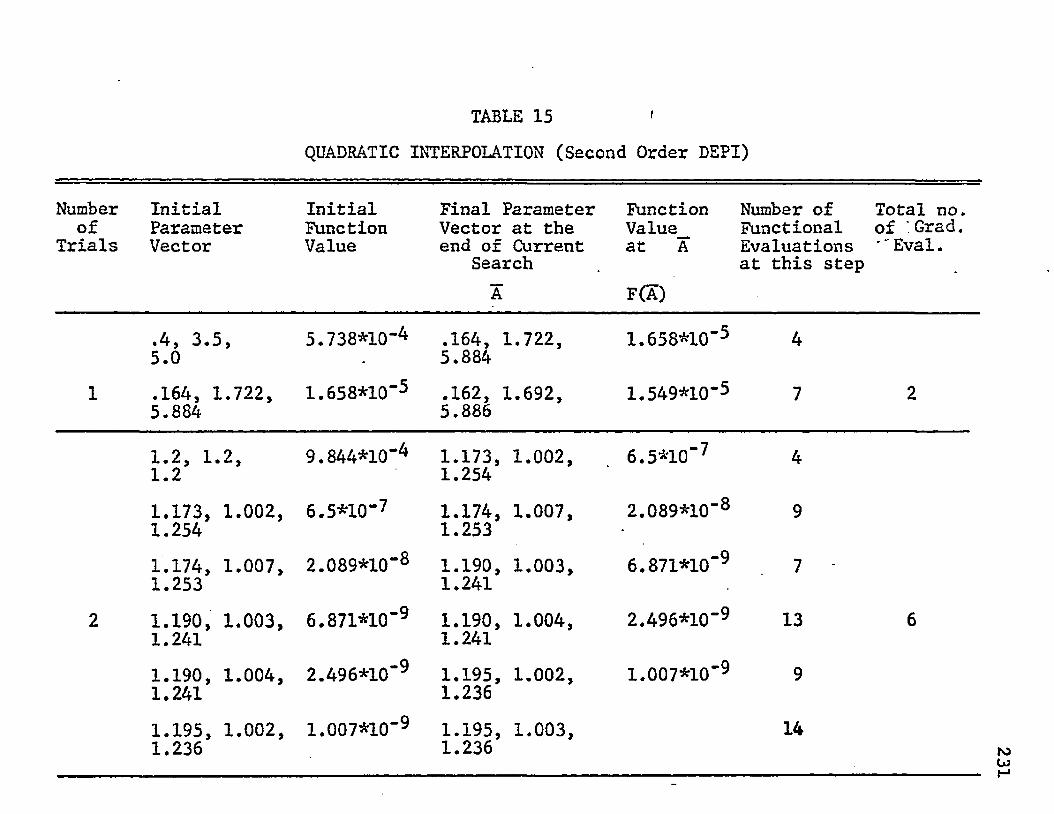
TABLE 15QUADRATIC INTERPOLATION (Second Order DEPI)

Numberof

TrialsInitialParameterVector

InitialFunctionValue

Final Parameter Vector at the end of Current

SearchA

Function Value_ at A

F(A)

Number of Functional Evaluations at this step

Total no. of ' Grad. ■" Eval.

.4, 3.5, 5.0

5.738*10“4 .164, 1.722, 5.884

1.658*10“5 4

1 .164, 1.722, 5.884

1.658*10‘5 .162, 1.692, 5.886

1.549*10”5 7 2

1.2, 1.2, 1.2

9.844*10“4 1.173, 1.002, 1.254

6.5*10"7 4

1.173, 1.002, 1.254

6.5*10“7 1.174, 1.007, 1.253

2.089*10"8 9

1.174, 1.007, 1.253

2.089*10“8 1.190, 1.003, 1.241

6.871*10"9 7

2 1.190, 1.003, 1.241

6.871*10~9 1.190, 1.004, 1.241

2.496*10“9 13 6

1.190, 1.004, 1.241

2.496*10“9 1.195, 1.002, 1.236

1.007*10'9 9

1.195, 1.002, 1.236

1.007*10”9 1.195, 1.003, 1.236

14

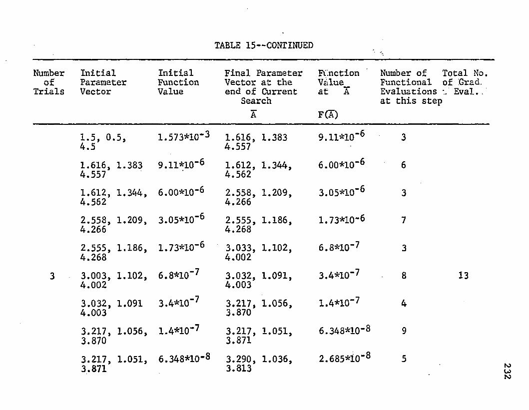
TABLE 15— CONTINUED

Numberof

TrialsInitialParameterVector

InitialFunctionValue

Final Parameter Vector at the end of Current

Search£

Function Value_ at A

F(A)

Number of Total No. Functional of IGrad. Evaluations *./ Eval. . at this step

1.5, 0. 4.5 5, 1.573*10*3 1.616,

4.5571.383 9.11*10"6 3

1.616,4.557

1.383 9.11*10"6 1.612,4.562

1.344, 6.00*10"6 6

1.612,4.562

1.344, 6.00*10"6 2.558,4.266

1.209, 3.05*10"6 3

2.558,4.266

1.209, 3.05*10"6 2.555,4.268

1.186, 1.73*10*3 7

2.555,4.268

1.186, 1.73*10“6 3.033,4.002

1.102, 6.8*10"7 3

3 3.003,4.002

1.102, 6.8*10"7 3.032,4.003

1.091, 3.4*10"7 8 13

3.032,4.003

1.091 3.4*10"7 3.217,3.870

1.056, 1.4*10“7 4

3.217,3.870

1.056, 1,4*10"7 3.217,3.871

1.051, 6.348*10-8 9

3.217,3.871

1.051, 6.348*10*3 3.290,3.813

1.036, 2.685*l0"8 5 232

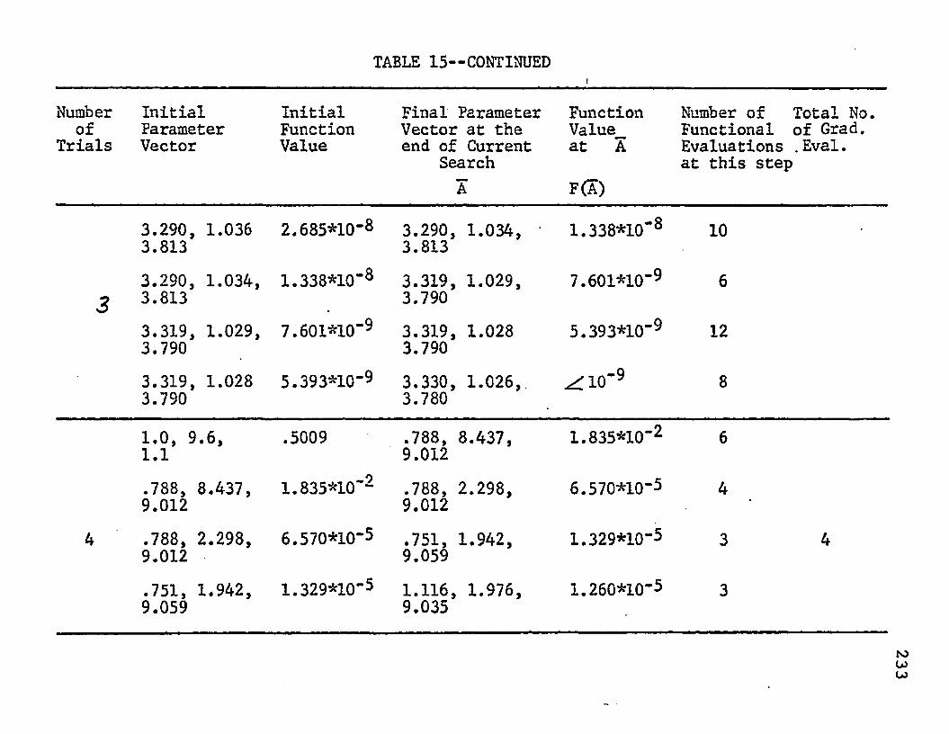
TABLE 15— CONTINUED

Numberof

TrialsInitialParameterVector

InitialFunctionValue

Final Parameter Vector at the end of Current

SearchA

Function Value— at A

F(A)

Number of Total No. Functional of Grad. Evaluations .Eval. at this step

3.290, 1.036 3.813

2.685*10"® 3.290, 1.034, 3.813

1.338*10*® 10

33.290, 1.034, 3.813

1.338*10“® 3.319, 1.029, 3.790

7.601*10“9 6

3.319, 1.029, 3.790

7.601*10"9 3.319, 1.028 3.790

5.393*10“9 12

3.319, 1.028 3.790

5.393*10"9 3.330, 1.026, 3.780

^IQ~9 8

1.0, 9.6, 1.1

.5009 .788, 8.437, 9.012

1.835*10“2 6

.788, 8.437, 9.012

1.835*10“2 .788, 2.298, 9.012

6.570*10-5 4

4 .788, 2.298, 9.012

6.570*10"5 .751, 1.942, 9.059

1.329*10-5 3 4

.751, 1.942, 9.059

1.329*10"5 1.116, 1.976, 9.035

1.260*10-5 3

233

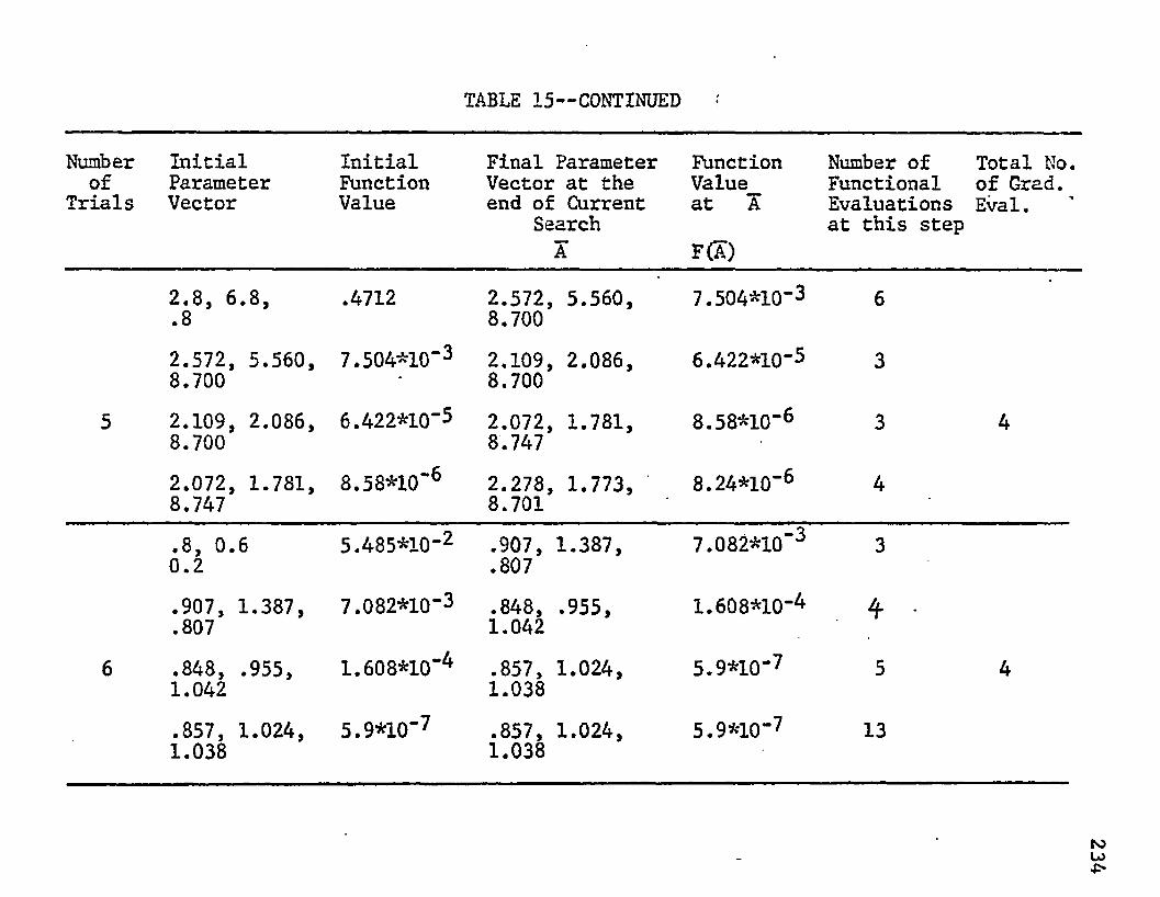
TABLE 15— CONTINUED

Numberof

TrialsInitialParameterVector

InitialFunctionValue

Final Parameter Vector at the end of Current

SearchA

Function Value at J.

F(A)

Number of Functional Evaluations at this step

Total No. of Grad. Eval.

2.8, 6.8, .8

.4712 2.572, 5.560, 8.700

7.504*10-3 6

2.572, 5.560, 8.700

7.504*10'3 2.109, 2.086, 8.700

6.422*10-5 3

5 2.109, 2.086, 8.700

6.422*10'5 2.072, 1.781, 8.747

8.58*10"^ 3 4

2.072, 1.781, 8.747

8.58*10'® 2.278, 1.773, 8.701

8.24*10"6 4

.8, 0.60.2

5.485*10-2 .907, 1.387, .807

7.082*10’3 3

.907, 1.387,

.8077.082*10*3 .848, .955,

1.0421.608*10-4 4 -

6 .848, .955, 1.042

1.608*10'4 .857, 1.024, 1.038

5.9*10“? 5 4

.857, 1.024, 1.038

5.9*10'7 .857, 1.024, 1.038

5.9*10"? 13

234

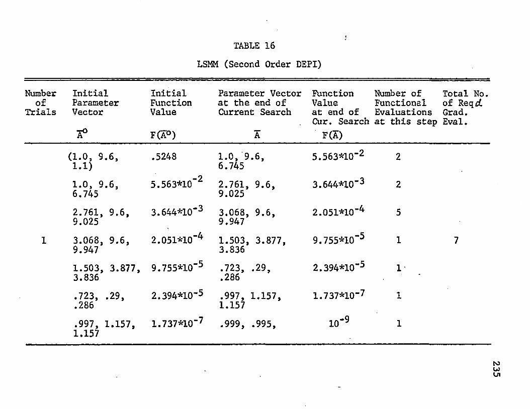
TABLE 16LSMM (Second Order DEPI)

Numberof

TrialsInitialParameterVector

InitialFunctionValue

Parameter Vector at the end of Current Search

Function Value at end of Cur. Search

Number of Functional Evaluations at this step

Total No. of Reqrf. Grad. Eval.

£° F(A°) J F ®(1.0, 9.6, 1.1)

.5248 1.0, 9.6, 6.745

5.563*10“2 2

1.0, 9.6, 6.745

5.563*10"2 2.761, 9.6, 9.025

3.644*10”3 2

2.761, 9.6, 9.025

3.644*10”3 3.068, 9.6, 9.947

2.051*10'4 5

1 3.068, 9.6, 9.947

2.051*10“4 1.503, 3.877, 3.836

9.755*10"5 1 7

1.503, 3.877, 3.836

9.755*10”5 .723, .29, .286

2.394*10”5 1-

.723, .29,

.2862.394*10*5 .997, 1.157,

1.1571.737*10“7 1

.997, 1.157, 1.157

1.737*10”7 .999, .995, 10”9 1

235

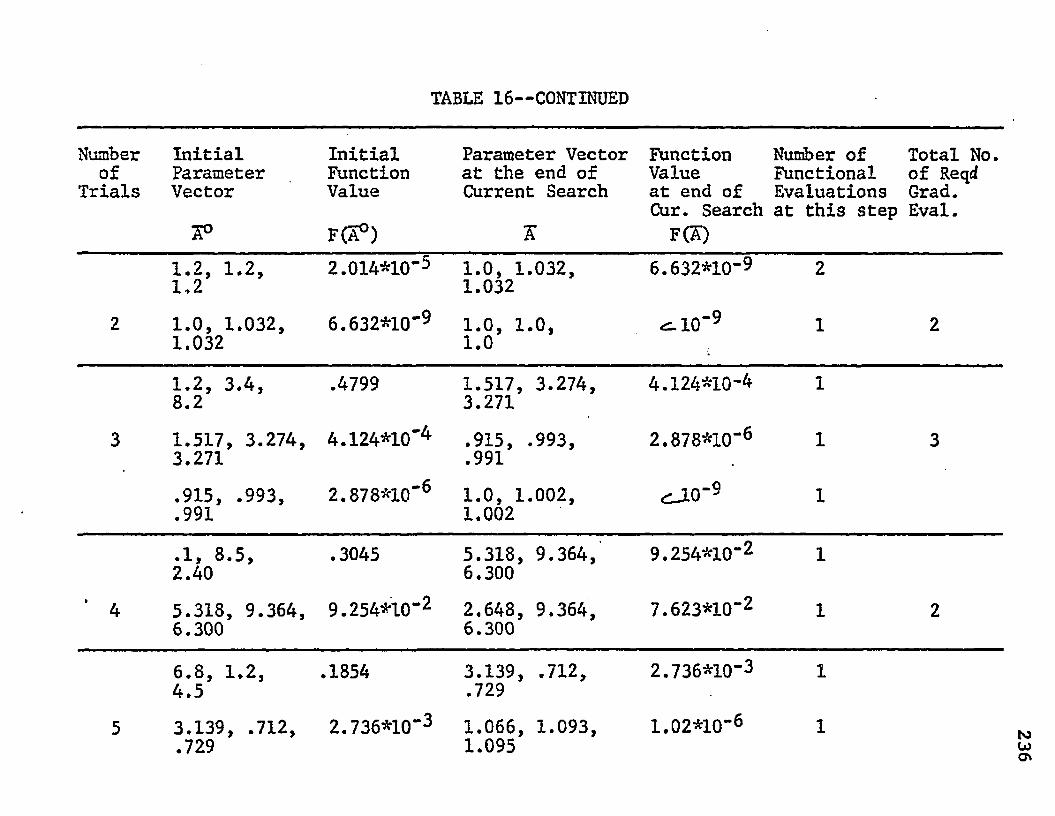
TABLE 16— CONTINUED

Numberof

TrialsInitialParameterVector

InitialFunctionValue

F(A°)

Parameter Vector at the end of Current Search

A

Function Number of Value Functional at end of Evaluations Cur. Search at this stepF ®

Total No. of Reqd Grad. Eval.

1.2, 1.2,1.2

2.014*10'5 1.0, 1.032, 1.032

6.632*10“9 2

2 1.0, 1.032, 1.032

6.632*10“9 1.0, 1.0, 1.0

^ 1 0 “9 1 2

1.2, 3.4, 8.2

.4799 1.517, 3.274, 3.271

4.124*10-4 1

3 1.517, 3.274, 3.271

4.124*10'4 .915, .993, .991

2.878*10“6 1 3

.915, .993,

.9912.878*10'6 1.0, 1.002,

1.002<lJL0"9 1

.1, 8.5, 2.40

.3045 5.318, 9.364, 6.300

9.254*10 1

‘ 4 5.318, 9.364, 6.300

9.254*10 2.648, 9.364, 6.300

7.623*10”2 1 2

6.8, 1.2, 4.5

.1854 3.139, .712, .729

2.736*10"3 1

5 3.139, .712, 2.736*10“3 1.066, 1.093, 1.02*10“6 1.729 1.095

236

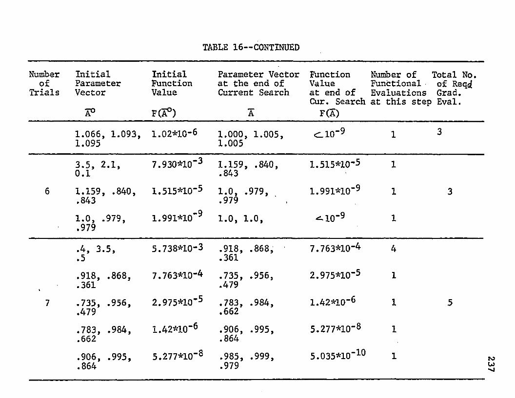
TABLE 16— CONTINUED

Numberof

TrialsInitialParameterVector

A°

InitialFunctionValue

F(A°)

Parameter Vector at the end of Current Search

X

Function Number of Value Functional at end of Evaluations Cur. Search at this stepF(A)

Total No. of Reqd Grad. Eval.

1.066, 1.093, 1.095

1.02*10-6 1.000, 1.005, 1.005

c^lO"9 1 3

3.5, 2.1, 0.1

7.930*10“3 1.159, .840, .843

1.515*10-5 1

6 1.159, .840, .843

1.515*10-5 1.0, .979, .979

1.991*10“9 1 3

■1.0, .979, .979

1.991*10"9 1.0, 1.0, ^ 1 0 “9 1

.4, 3.5,

.55.738*10*3 .918, .868,

.3617.763*10-4 4

t.918, .868, .361

7.763*10-4 .735, .956, .479

2.975*10"5 1

7 .735, .956, .479

2.975*10'5 .783, .984, .662

1.42*10-6 1 5

.783, .984,

.6621.42*10“6 .906, .995,

.8645.277*10"8 1

.906, .995,

.8645.277*10"8 .985, .999,

.9795.035*10"10 1 237

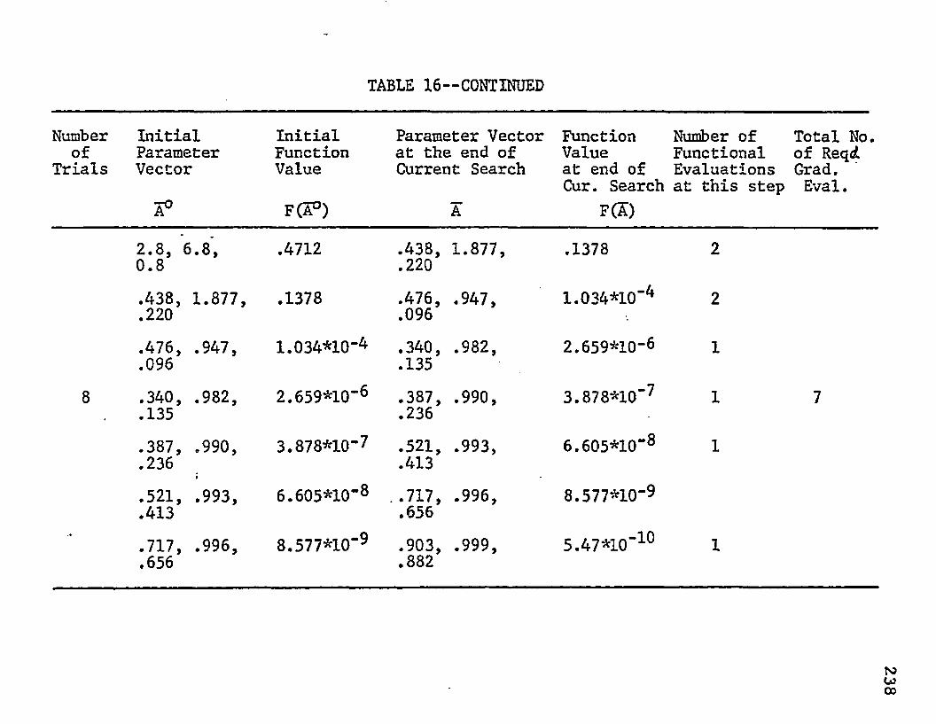
TABLE 16— CONTINUED

Numberof

TrialsInitialParameterVector

A0

InitialFunctionValue

F(A°)

Parameter Vector at the end of Current Search

A

Function Value at end of Cur. Search

F ®

Number of Functional Evaluations at this step

Total No. of Reqd Grad. Eval.

2*8, 6.8,0.8

.4712 .438,.220

1.877, .1378 2

.438, 1.877,

.220.1378 .476,

.096.947, 1.034*10"4 2

.476, .947,

.0961.034*10-4 .340,

.135.982, 2.659*10-6 1

8 .340, .982, .135

2.659*10"6 .387,.236

.990, 3.878*10~7 1 7

.387, .990,

.2363.878*10-7 .521,

.413.993, 6.605*10“8 1

.521, .993,

.4136.605*10"® ..717,

.656.996, 8.577*10‘9

.717, .996,

.6568.577*10“9 .903,

.882.999, 5.47*10"10 1

238

APPENDIX C

APPENDIX C

This appendix describes details of the computer program developed for automatic identification of both the onset and end of ventricular diastole, as defined in Chapter VI. Figure 1 shows a representative sketch of the actual diameter recording, D(t), from a single cardiac cycle. Point A represents the onset of diastole and point C the end of diastole. The time period A to D corresponds to the period of a cardiac cycle. It was noted in the recordings that after some intervals of time the diameter curve stayed relatively constant (Point B).In a strict peak and/or valley determining algorithm, the computer may incorrectly identify the point B as the maxima for the given cycle. In order to avoid this error a comparison based on the magnitude of the difference between two successive sample points was incorporated into the program. In terms of digital output it was observed that this magnitude was of the order of 20.

A brief description of the program used Is detailed with reference to the computer flow chart (Figure 2). In the program a counter JJ is initialized. JJ is used to keep account of the number of records processed. In case JJ reaches the number 450, signifying the last record, the computations are stopped. Otherwise, data is read from

240

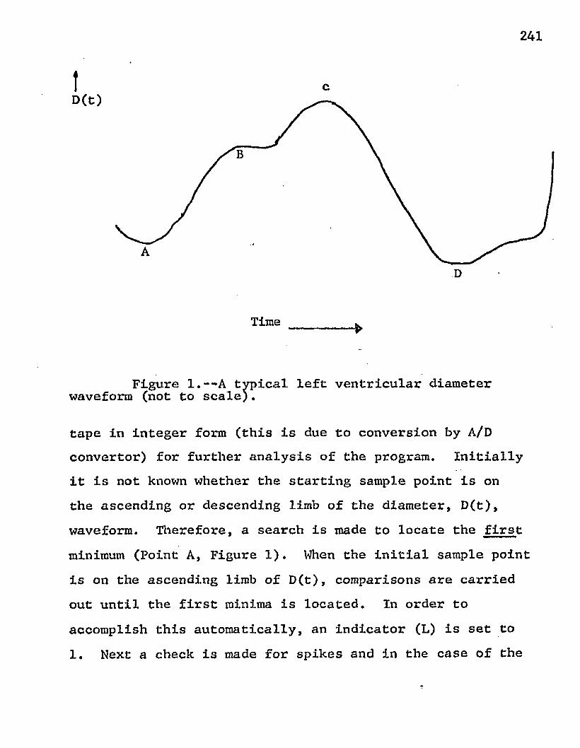
D

Time _________^

Figure 1.— A tvpical left ventricular diameter waveform (not to scale;.

tape in integer form (this is due to conversion by A/D convertor) for further analysis of the program. Initially it is not known whether the starting sample point is on the ascending or descending limb of the diameter, D(t), waveform. Therefore, a search is made to locate the first minimum (Point A, Figure 1). When the initial sample point is on the ascending limb of D(t), comparisons are carried out until the first minima is located. In order to accomplish this automatically, an indicator (L) is set to1. Next a check is made for spikes and in the case of the

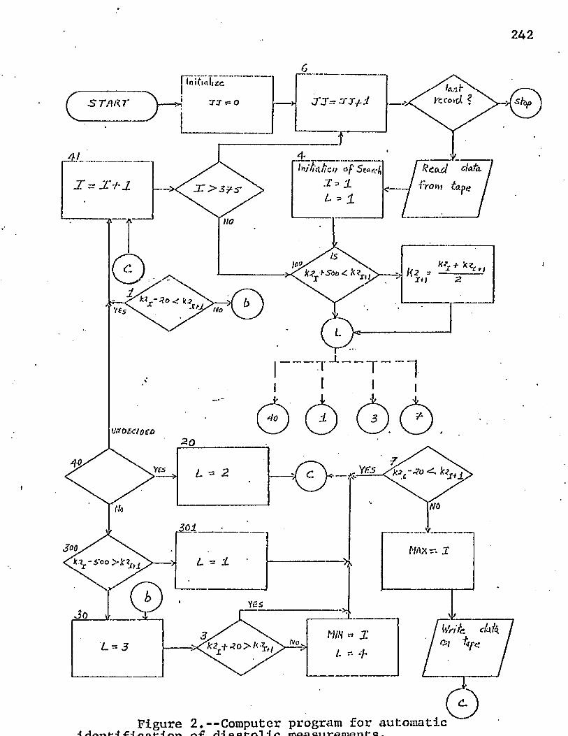
242

6

wo

jr+jNoV«5

, JL” 7! '

/VO

3ook*x-‘,-oo>k?Xti

*>:Jo

MW « XL - 3

Figure 2.— Computer program for automaticn n f- j nn dd t-r t l ■( m ail Cl I t'AnlO n t* Q .-I A

243

presence of a spike a simple averaging is used to generate k^Url* (k2 is the integer identifying name used from D(t) sampled points.) Depending on the value of L control is transferred to blocks 40, 1, 3, or 7 (these numbers refer to FORTRAN address of the blocks). In block 40 a check is made whether or not the sample point k2x is on the ascending portion of the curve using the following equation:

(C.l) Is k2x - 20<^k2I+x ?If the answer to the above querry is "yes,1' control is transferred to block 20 where L is set equal to 2 to indicate that k2j is on the ascending portion of the curve. The control is then transferred to block 41 to continuethe search for the first maxima.

If the answer to equation C.l is "no," then k2x is onthe descending portion of the curve. A check is made Inblock 300 for false start on a spike. In case this happens control is transferred to block 41 with L set to 1 to beginthe search process. Otherwise, L is set to 3 to indicatethat the search Is continuing for the first minima. The minima Is located by use of the following:

(C.2) Is k2x + 20‘?'k2X4.i ? (block 3)If the answer to equation C.2 is "yes," the search is continued by transfer of controls to block 41. A minima is located when k2j+20^k2x+x. This point is marked MIN andcontrol is returned to block 41 with L set to 4.

244

If the answer to question C.l is that K2j-20 =• K2-j-+ (indicating a possible flat surface corresponding to point B, Figure 1) then control is transferred to block 41 to increment I. Because no decision is made at such sample points, false starts or stops on point B are avoided.

Block 1 signifies that the sample point I is located on the ascending limb of the D(t) curve and that this is the search for first maxima (La2), The question asked at this stage is:

(C. 3) Is k2x - 20d.k2I+1 ? (block 1)A negative answer to question C.3 confirms the location of the first maxima and the search is continued to locate the minima by setting La3 and transferring controls to block 30. Otherwise, I is incremented and question 3 is repeated.

Block 7 signifies that the minimum (MIN) of the D(t) waveform for the current cardiac cycle has been located. In order to locate the maxima in this cycle the following comparison is made:

(C.4) Is k2I - 20^-k2Ihl ?If k2j-20 is less than k2j+^ then the maxima has been located and the sample point is termed MAX. Otherwise,I is incremented and question C.4 is repeated.

Once MIN and MAX have been identified (corresponding to points A and C of Figure 1) the output between these

245

two sample points is stored on a magnetic tape. The corresponding pressure points are also stored in a vector k3 (corrections are made for the spikes).

After the successful location of MAX, control is transferred to block 41 to continue the search to locate the minima of the next cardiac cycle after setting L to 3. Also, JJ is incremented by 1 to signify that a record has been processed.

This procedure is repeated until all the records have been analyzed. The actual coding is included on the following pages for possible use with other problems.

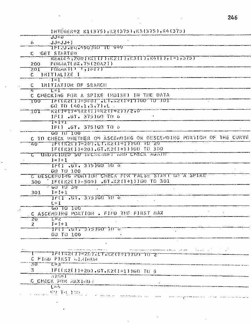
246

1NTEGER* 2 K1 t 3 V5 ) , K2 ( 376 ) , K3 ( 3 7 f> ) , K4 ( 37:>) -JCFTT-------------------- 1

6 J J = J J + ]-------------- j T r j x ^ r ^ f s o n r , c r n r youC GET S T A R T E D ______ _ _________________________________________________

iTFnT'T7!-TTooTfiZTTTTTiTFTTTTi37*3"*} ? R'* 1I ) » i = 1 1 3 /y )200 FOili-iAT( OX , 73 ( 20 A2 ) )

ToT~ FTJiCtv\Tl i r~TloT~nC I N I T I A L I Z E I *

C I N I T I A T I O N OF SEARCH m -C CHECK I MG FOR A SPI KE ( N O I S E ) I N THE DATA

t o o ----- r F rn c rn t ::73t o t - n T ;T m ~ T i'T G !T "T u ~ iT ri ~GO TO ( 4 0 i 1 » 3 i 7 ) » L .

TO T-----TCZtTOTsT K2 (T ) '-TTH T *' 2T)7'2TT<I F ( I . G T . 3 7 3 ) GO TO 6

--------------r -r -n .-----------------------------------------------------------------------------------------------------------------I F ( I . G T . 3 7 5 ) GO TO o

Girrrrnra----------------------------------------------C TO CHECK WHETHER OH ASCENDING OK DESCENDING PfJR' I IOM OF THE CURVE

T O T R " n T 2 T T T ^ a '7 U T 7 T < 2 T T T n T G n “T 0 “ Zn ~~I F ( ( K2( I ) * 2 0 ) . GT .1' 2 ( I +1 ) )GD TO 3 0 0

~C Ui-;U i C i U c O SU r i T ’AE.ibi-7 RTiTTTTrTETK nGTniv

IT T I . G Y . 3 7 3TgTj it) oGO TO 100

C OE SC E i'T J lT T - iJ L f iT l uTT'CI'-rHTK T P R "'FA‘L St: S i /-■!< t un" a TPT7C F 3 0 0 I F ( ( K 2 ( I ) - 5 0 0 ) . G T . K 2 U + 1 ) )GU TD 3 0 1un I U 3 03 0 1 1 =1 +1

I F ( I . G T . 3.7 5 ) GO ‘ID o L= 1G'u i u l oO ~ ‘

C ASCENDJMG PORT I OH . F I HD THE F I R S T MAXTu l.~ 22 1=1+1

-------------- T F ’tT .G T '. ,3 7 jrrG 0 ” 1 Cr~uGU TU 100

r TFt tto ? h t -p.ot; r r . i r z r m T r G n - n n —C F l i i U F I R S T i-i 1.11 lii.Ji'i

3 1 Ft ( X 2 ( 1 )-:-?.Q ) . G T . K 2 ( I +1 ) )Gfl To 5

-*l j ” I “ " ”C CHECK r I ! K MAX I : iU i__________________

1:1! T‘J ] Of;

247‘3 J « I + 1

I r (. J . G T . 3 7 5 JGO TO 6GO IU 1U0I F ( ( K2( 1 ) - 2 0 ) • L T . K 2 { 1 M ) ) GO TO 8

GO TO S1~s-----------r= r+ ~ r—

GO TO 100 T70 Xu J=T-: 7 r: « r a a •I F ( K 3 ( J ) + 50 0 . L T . K 3 ( J * 1 ) ) K3 ( J + i ) * ( K3( J ) -J-K3 ( J + 2 ) ) / 2 . 0

_r i 'T !3 i^ )" -T -o u ™ i:0 T ''3 r 3 iT i^ T r ) i ; '3 '( ';T -n 'r := '(it'3 'rj')^rK3'(Tn^ r ) ' 7 7 7 v ' I F ( K 2 ( J J - 5 0 0 . L T . K 2 ( J + X ) ) K 2 ( J + l ) = ( K 2 ( J ) * K 2 ( J + 2 ) ) / 2 . 0

IT T C-O^T-rFfU£ ---- -----------------------------------------------------WRI T E ! 6 , 1 0 5 ) ( K 2 ( J ) • K 3 { J ) » J “ O IM i i-i AX )

“LtTD F tjn r r7 r tt-*— '-T_,i r 3 HT t 'r j “ i ----------------------------------------WRI T E ! 3 ) , i l U , ; i A X

---------------n K T T -H r r r (t.z i t l i t o -TTiTnTrs/C-)-------------------------WRI T E ! 3 ) ( !s3 ( J ) j J =!vi 1»'!» mAX )

---------17^3--------------------------------------------GO TO 1 0 0

W S 5 T C T P - - - - - - - - - - - - - - - - - - - - - - - - - - - - - - - - - - - - - -EMU7?c

I

i

APPENDIX D

REVIEW OF OPTIMIZATION TECHNIQUES

l

248

REVIEW OF OPTIMIZATION TECHNIQUES

This appendix contains a brief review of optimization theory as applied to the DEPI problem. The material reported herein is taken from a number of books"*® andpapers^ and is intended for familiarization of the reader to the basic ideas in optimization. In the Interest of brevity, only pertinent details are given and the interested reader is referred to the referenced material for complete theoretical justifications.

Optimization, by definition, is concerned with finding "the best" solution to a given problem. In this context best refers to a solution which is better than all others with respect to a specified performance criteria (measure), subject to a known set of conditions. An "optimization technique" is a step-by-step description of the process used in deriving the "best" solution to a given problem.Many different optimization techniques have been developed due to the multitude of problem formats, each of which requires a distinct solution approach. For a given problem a particular process may be the most efficient (i.e., requiring the minimal amount of time and effort to derive the best solution) but it may not be as efficient for other problems.

249

250

With the availability of various optimization methods it is felt that the most desirable attributes of each way be combined to yield a "general optimization technique." With this "general optimization technique" the amount of time and effort involved in determining the best solution may be reduced below that required using each method separately.

A number of books have been devoted to the problemsC£ C 7of optimization and optimizing techniques. 9 However,

for the purposes of this study certain techniques have special significance and these are briefly reviewed in this appendix.

In general, optimization methods may be classified under the following broad categories:

1. Indirect (analytic) search method2. Direct search method

Indirect Search MethodsThe mathematical properties of the objective function

are utilized to locate the optimum value. For example, in the case of well-defined objective functions of a single parameter the optimum may be located by studying the function behavior of its stationary points.

In the case of functions of several parameters the stationary point(s) are located at parameter values where the first partial derivatives of the function, with respect to

251

each parameter, vanish. Indirect methods require the objective function and Its partial derivatives to be available in terms of analytical expressions. The numbers of problems that may be studied using indirect methods is rather limited due to the many difficulties associated with obtaining analytic expressions for complex phenomena.

Direct Search MethodsThese methods, in principle, do not depend upon the

mathematical behavior of the objective function. However, it will be seen that the more efficient of these methods utilize some of the analytic concepts. The basic guiding philosophy in all direct search techniques is to find the optimum solution by computation and comparison of function values. Recourse to machine computation (analog or digital) becomes mandatory for problems involving complex functional evaluations.

Direct search techniques may be categorized based on:1. Nature of the problem2. Nature of performance criteria and constraints3. Type of available data4. Type of parameter values

Nature of the ProblemThe "search methods" based on the nature of the

problem can be subdivided into the following:

! 252I

1. Nonsequential methods I2. Sequential methods j

iNonsequential methods.— These methods deal withi

problems in which a solution is generatedjwithout considering!

any other prior solutions. Therefore, these methods arei

non-iterative. From an "efficiency" viewpoint the non­sequential search methods are, in generalj inferior to the sequential methods.Nonsequential search methods aregenerally used to provide starting points search.

for a sequential

Sequential methods.--In these methods information from past solutions is used in order to determine the future solutions. The methods differ in the manner in which past information is utilized. Since the sequential methods, by definition, learn to move toward an optimum solution they are generally more efficient than nonsequential methods which are heavily dependent on chance. It must be noted that the sequential methods are based on the assumption that the function behavior is unimodal (i.e., only one optimum point) in the region under consideration. In case the objective function is multimodal (i.e.,‘ several optimum points lie in the specified region of parameter values), the sequential search methods will converge to a particular optimum point depending on the starting parameter values.

253

When this happens, it is possible that the lowest function value, called global minima, (in case of minimization problems) in the region under study may not be obtained. As McGheepoints out this is very likely to occur in the case of DEPX problems. Unfortunately there are no available methods which enable one to deal with the global minima problem. Limited assurance of a global minima may, however, be obtained by repeating the search using a different starting value and noting the final function value. The lowest function value among these may be termed global minima for the region under study. Since global minima in case of DEPI provides the best fit, as far as model matching is concerned, efforts must be expended toward its location.

Therefore, in this dissertation a non-sequential method (random search) has been used in conjunction with the sequential methods to locate the "global minima" in a specified region (Chapter V).

Nature of Performance Criteria and Constraints

Depending on the nature of the performance criteria and the constraints on parameter values, the search methods may be classified as:

1, Linear Programming Problem.-»When both the performance criteria and the constraints are linear functions the optimization becomes a linear programming

254

problem. This particular case has been fully solved by Danzig.^

2. Nonlinear Programming Problem.--In case the performance criteria and/or the constraints are nonlinear*

C QThe DEPI problem in general falls under this category,since the performance criteria may not be a linearfunction of the parameters.

72Bellman has generalized both the linear and non­linear programming problems into a multistage decision process. This generalized form is known as "dynamic programming." In this dissertation, attention will be limited to the various methods for achieving an optimum value and, therefore, the theoretical aspects of dynamic programming will not be discussed (an excellent referencesource for the interested reader is Bellman's book on

72Dynamic Programming ).

Type of Data Available .Depending on the type of available data, the search

methods may be classified as:1. Continuous search.--The given performance

function is a continuous function of parameter(s).Analog computers are particularly useful for problems of this type; however, since an analog computer itself may be simulated on a digital computer, this distinction is rather arbitrary.

2552. Discrete search*— The objective function is

evaluated only at discrete values of parameter(s).Most search methods utilizing numerical computations fall under this category.

Types of ParametersDepending on the nature of parameters of the

9objective function, the search methods may be classified as:1. Real parameter search.--When the parameters

may take on any real value in the region under study.2. Integer parameter search.— When the parameters

are constrained to be integers in the region of interest. Beale^ provides an excellent review of current literature in this area.

Search Methods Applicable to DfiPt Problem

In the case of DEPI problem under consideration, the parameters are real variables and the objective function is computed as a discrete function of the following variable:

1. The observed data points YT2. Model response YUIt is difficult to write an analytic expression for

the objective function which characterizes the function behavior with respect to the parameters of the model. Therefore, further discussion will be limited to direct

256

search techniques which utilize discrete data and real parameter values with numerical evaluation of objective function.

Specific search methods which provide background information about those considered in this dissertation (Chapter IXX) have been subdivided into the following classifications based on the number of unknown parameters (dimensions in parameter space).

1. One-dimensional search methods2. Multidimensional search methods

One-dimensional Search MethodsThese methods are applicable for optimization of

functions of a single parameter. Consideration of one­dimensional techniques is important since many of the efficient multidimensional search methods involve, at various stages of computation, an optimization along a particular direction. Of the many available one-dimensional search methods, the following have been selected on the basis of their application to the solution of the multidimensional problem at hand. These are:

1. Newton-Raphson search2. Search by Golden Section3. Quadratic Interpolation (QUAD)4. Pierre's Interpolation Scheme (PIS)

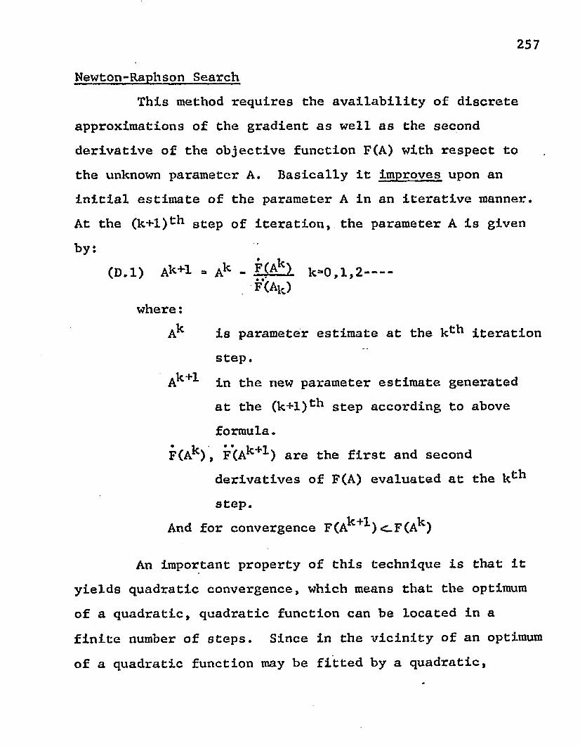
Newton-Raphson SearchThis method requires the availability of discrete

approximations of the gradient as well as the second derivative of the objective function F(A) with respect to the unknown parameter A. Basically it improves upon an initial estimate of the parameter A in an iterative manner. At the (k*t*l)tk step of iteration, the parameter A is given by:

(D.l) Ak+3- =* Ak - SfofeX k“0 ,1,2---F(Ak)

where:A^ is parameter estimate at the ktk iteration

step.A^+ in the new parameter estimate generated

at the (k+l)tk step according to above formula.

F(A^), F(A^+ ) are the first and secondderivatives of F(A) evaluated at the ktk step.

And for convergence F(A^+^) c.F(A^)

An important property of this technique is that it yields quadratic convergence, which means that the optimum of a quadratic, quadratic function can be located in a finite number of steps. Since in the vicinity of an optimum of a quadratic function may be fitted by a quadratic,

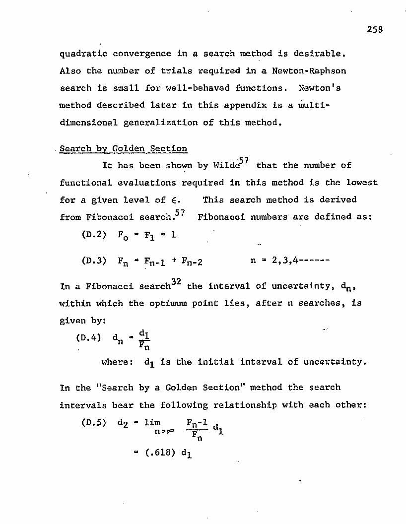
258

quadratic convergence in a search method is desirable.Also the number of trials required in a Newton-Raphson search is small for well-behaved functions. Newton's method described later in this appendix is a multi­dimensional generalization of this method.

Search by Golden Section57It has been shown by Wilde that the number of

functional evaluations required in this method is the lowestfor a given level of €. This search method is derived

57from Fibonacci search. Fibonacci numbers are defined as: (D.2) fd - FX - 1

(D.3) Fn » Fn-i + Fn-2 n - 2,3,4.....32In a Fibonacci search the interval of uncertainty, dn>

within which the optimum point lies, after n searches, is given by:

(D.4) dn =*n

where: d- is the initial Interval of uncertainty.

In the "Search by a Golden Section" method the search intervals bear the following relationship with each other:

(D.5) d2 - lim Fn-1 ,n Tf 1Fn

- (.618) d l

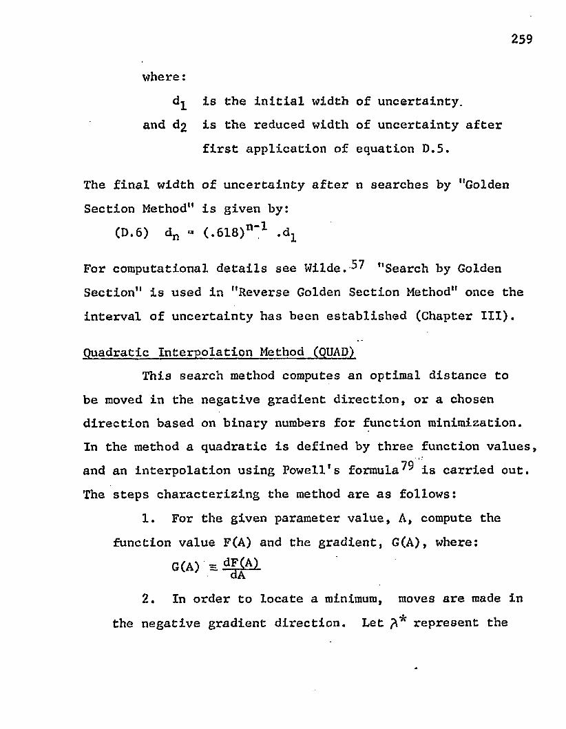
where:d^ is the initial width of uncertainty,

and d2 is the reduced width of uncertainty after first application of equation D.5.

The final width of uncertainty after n searches by "Golden Section Method" is given by:

(D.6) dn - (.eiB)0-1 ,dl

For computational details see Wilde.^ "Search by Golden Section" is used in "Reverse Golden Section Method" once the interval of uncertainty has been established (Chapter III).

Quadratic Interpolation Method (QUAD)This search method computes an optimal distance to

be moved in the negative gradient direction, or a chosen direction based on binary numbers for function minimization.In the method a quadratic is defined by three function values, and an Interpolation using Powellrs f o r m u l a i s carried out. The steps characterizing the method are as follows:

1. For the given parameter value, A, compute the function value F(A) and the gradient, G(A), where:

G(A) s2. In order to locate a minimum, moves are made in

the negative gradient direction. Let represent the

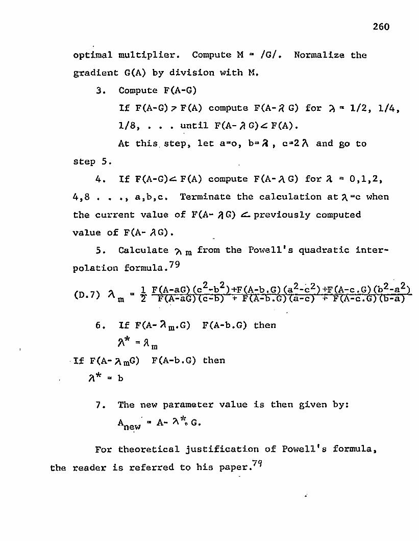
260

optimal multiplier. Compute M * /G/. Normalize the gradient G(A) by division with M.

3. Compute F(A-G)If F(A-G)?F(A) compute F(A-^G) for ^ - 1/2, 1/4, 1/8, . . . until F(A- /} G)<C F(A).At this step, let aao, b=* % , c=“2/\ and go to

step 5.4. If F(A-G)*d F(A) compute F(A-AG) for Z » 0,1,2,

4,8 . . a,b,c. Terminate the calculation at Bc when the current value of F(A- flG) <£-previously computed value of F(A- /IG).

5. Calculate ^ ra from the Powell*s quadratic inter­polation formula.

-,x ^ 1 F(A-aG)(c2-b2)+F(A-b.G)(a2-c2)+F(A-c.G)(b2-a2)( *7> 7 '"F"(A-aG)'(c-t;) > F(£-T7g) (a-c) + T(A-c'.G) (b "aT'

6. If F(A-2m .G) F(A-b.G) then

If F(A-/\mG) F(A-b.G) thena* = b

7. The new parameter value is then given by:A„ « A- G. new

For theoretical justification of Powell's formula,•70the reader is referred to his paper.

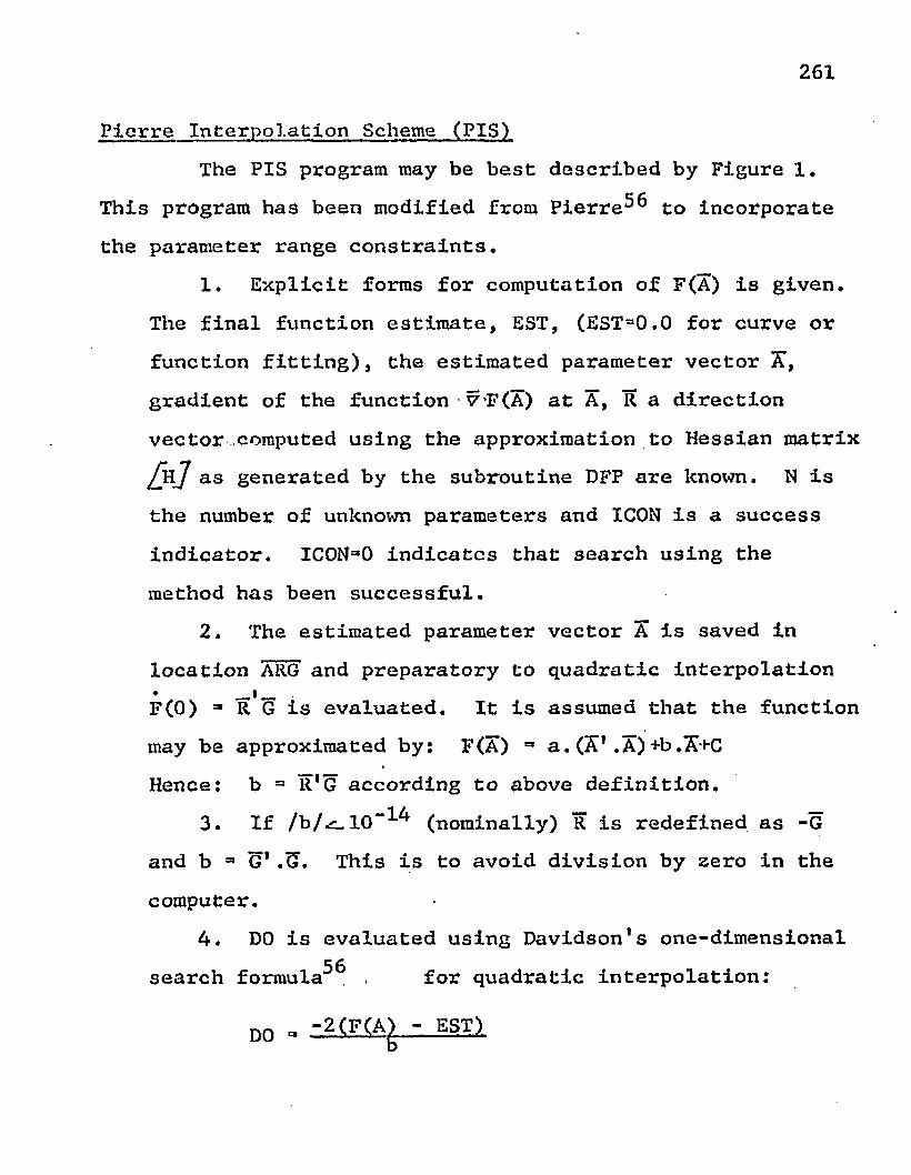
261

Pierre Interpolation Scheme (PIS)The PIS program may be best described by Figure 1.

This program has been modified from Pierre^ to incorporate the parameter range constraints.

1. Explicit forms for computation of F(A) is given. The final function estimate, EST, (EST^O.O for curve or function fitting), the estimated parameter vector X, gradient of the function V'F (A) at A, R a direction vector computed using the approximation to Hessian matrix /WJ as generated by the subroutine DFP are known. N is the number of unknown parameters and ICON is a success indicator. IC0N=*0 indicates that search using the method has been successful.

2. The estimated parameter vector A is saved in location ARG and preparatory to quadratic interpolation• . i _F(0) ** R G is evaluated. It is assumed that the functionmay be approximated by: F(A) a a.(S'.A)+bHence: b =* R'G according to above definition.

3. If /b/^-10“^ (nominally) R is redefined as -Gand b =■ G 1 .(?. This is to avoid division by zero in thecomputer.

4. DO is evaluated using Davidson's one-dimensional56search formula for quadratic interpolation:

DO - -2(F(A|> - EST)

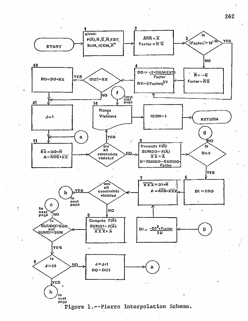
262

given: F(A),R,G,N,GST, SUM, ICON, A°

ARG = A Factor ~ It 'G YES

S T A R T

NO

DO = -2«(SUM-ES*n) Factor

RX=(lFaetor|)1/2 *R = - G

Factor = R'GYES < -----

NO 'fromnextpage

RangerViolators ICON— IJ = 1

r e t u r n

YES

Compute F(A)SUMDQ— F(A)

X X = AU=SUMDO~SUMDO

Factor

all v constraints violated

X X -D O -RA -A R G + X X

YES

/ n r o \ all \

constraints violated

X X X = D I * R

A =ARG+XXXYES DI " 2DO

nextpage1° \ . J

nextpage NO

NO

Compute F(A) SUMD1= F(A)

X X X = A'5UMDO>SUM

andUMD1=>SUM x

DI — ~D0 «Fnctor «$-2 U

YES

NOJ > 2 0

'YES

Figure 1.--Pierre Interpolation Scheme.

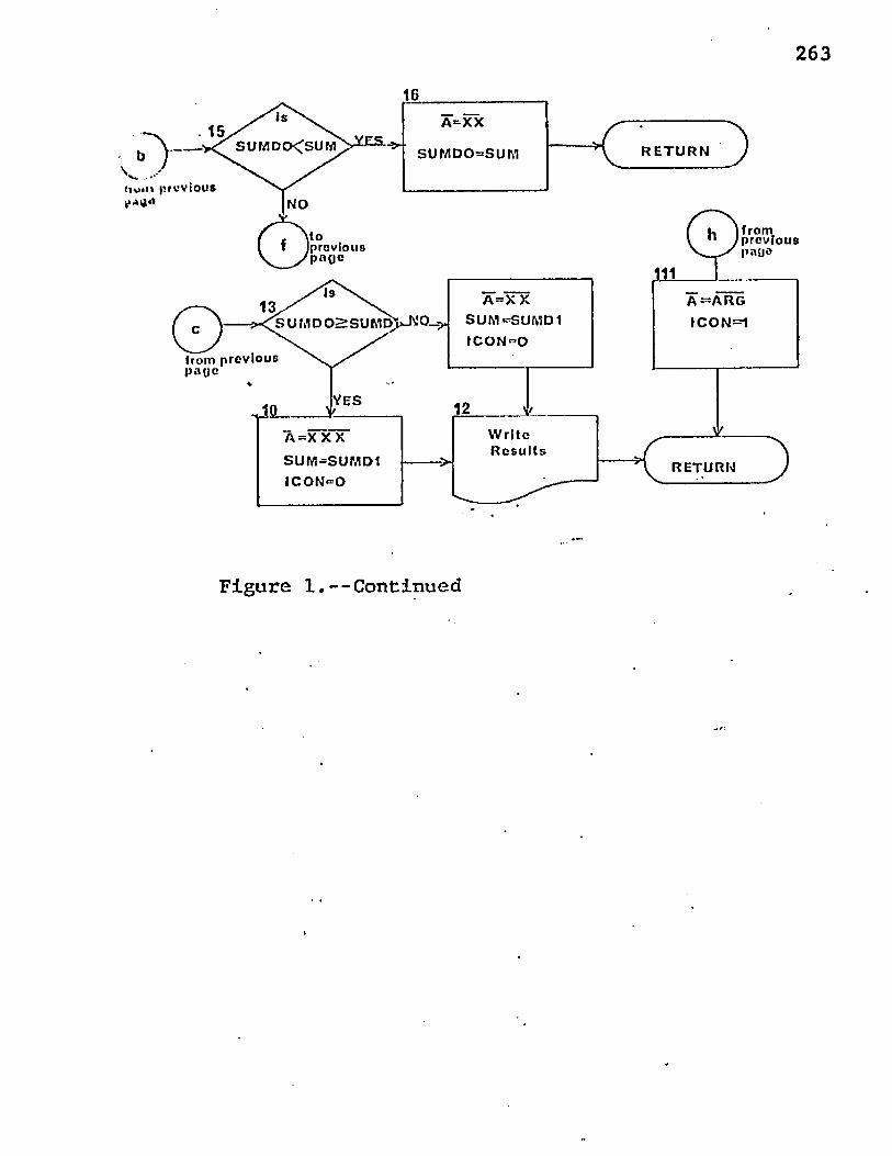
263

R E T U R NSUMDORSUM

NO

frompreviouspane

111A = X X

SU M -SU M D1 IC O N -O

S U M D o s s u m d >-J^Q->

from previous pa«c

YES

A =X X X

SU M -SU M D1IC 0 N = 0

W riteResults

RETURN

Figure X.— Continued

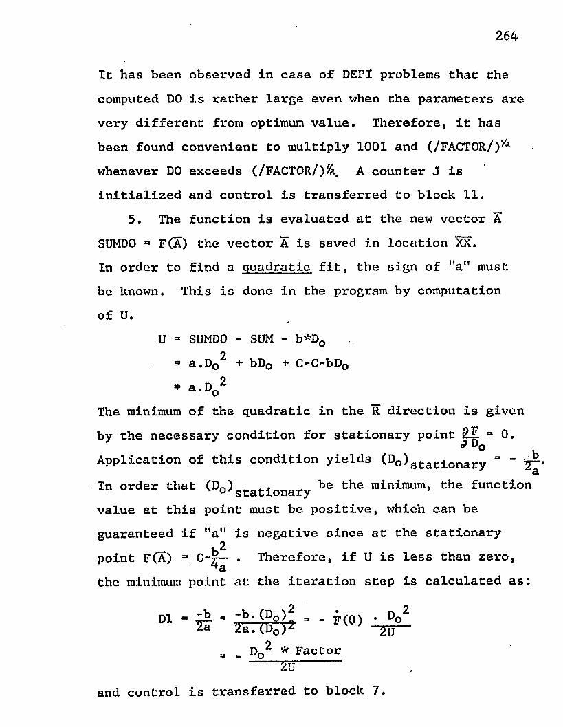
264

It has been observed in case of DEPI problems that the computed DO is rather large even when the parameters are very different from optimum value. Therefore, it has been found convenient to multiply 1001 and (/FACTOR./)^ whenever DO exceeds (/FACTOR/)&, A counter J is initialized and control is transferred to block 11.

5. The function is evaluated at the new vector A SUHDO “ F(A) the vector A is saved in location XX.In order to find a quadratic fit, the sign of "a” must be known. This is done in the program by computation of U.

U - SUMDO - SUM - b*D0 2a a.D0 + bD0 +■ C-C-bD0

* a.D02The minimum of the quadratic in the R direction is given by the necessary condition for stationary point =* 0. Application of this condition yields (D0)stationary “ " 3P-*In order that (D«) be the minimum, the function° stationaryvalue at this point must be positive, which can be guaranteed if "a” is negative since at the stationary point F(A) a C“y~— . Therefore, if U is less than zero, the minimum point at the iteration step is calculated as:

D1 " & ■ ■ * * (0) ^a - D0^ ^ FaCt°r

and control is transferred to block 7.

265

6. If U is positive, the minima cannot be guaranteed at this Iteration step. A larger step in the directionR is taken to generate a possible lower function value.

7. The change vector XXX » D1*H is added to the initial parameter vector ARG and a check is made of constraint violations. In case all constraints are violated, control is transferred to point b.

8. If all range constraints are not violated, the function is evaluated at F(A) and saved in location SUMD1. A is also saved in location XXX. If both SUMDO and SUMD1 are greater than initial function value, another iteration is attempted by transferring control to block 9.

Otherwise control is transferred to point C for check on the lower of the two computed values SUMDO,SUMD1.

9. If J^20, then ICON is set to 1 to indicate the failure of the method to minimize in 20 iteration steps. The initial parameter vector and function value are returned to the calling program.

10. Since SUMDO Z~ SUMD1, the lower function value and associated parameter vector XXX are returned as the new estimates. ICON is set to zero to indicate success of the method at this iteration step and control is trans­ferred to block 12.

266

11. The parameter change vector is computed and the new parameter vector A is generated. In case all range constraints are violated, control is transferred to block 14 to indicate range violations and failure of the method.

12. A success message is written and the results are returned to calling program.

13. A comparison is made between SUMDO and SUMD1 values if SUMDO is less than SUMD1 the new parameter estimates are:

£ » XX SUM - SUMDO

and-control is transferred to block 12.14. No further computation is done due to range

violations. ICON is set to one to indicate failure of the method. Control is returned to calling program.

Multidimensional Search MethodsIn the case of optimization of objective functions

of a single parameter, one is reasonably certain of locating an optimum value within a given range. If the function is "unimodal" in the allowed region, then only one optimum exists and may be easily found using either direct or indirect techniques. In case the function behavior is "multi-modal" then starting at different search points the

267

whole region of interest may be explored to locate the "global optimum point." In either case the effort required to find the optimum is not very time-consuming. However, as the number of unknown parameters increas the effort involved in locating the optimum increases considerably.This has been very aptly termed as the "curse of dimension­ality" by B e l l m a n .72 The chief problems due to increase in dimensions are:

1. Because of the presence of interacting parameters the visualization of function behavior becomes difficult especially for problems involving more than two para­meters. This hampers the choice of starting parameter values.

2. As the number of parameters increase, the number of optimum points often increases.

3. The size of the region defined by the parameter values, in which the search is to be conducted, increases considerably with increasing number of parameters.

This may be illustrated by the following example. Consider a unidiraensional minimization problem with the range of parameter being O ^ A ^ l . The size of uncertainty is given by 1. Suppose that the minimum is known to lie in the range O^A^.5. Therefore, the original size of uncertainty may be reduced by 50 percent to 0,5.

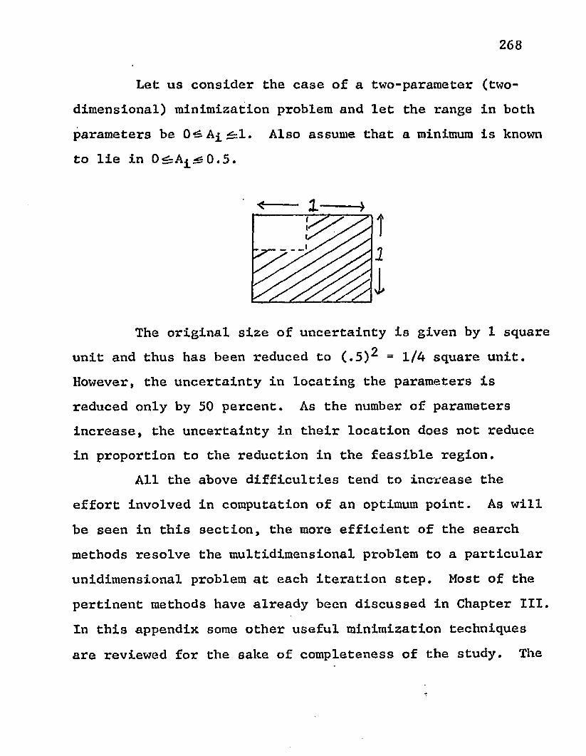
268

Let us consider the case of a two-parameter (two- dimensional) minimization problem and let the range in both parameters be 0^A£^=1. Also assume that a minimum is known to lie in 0 A^-s 0.5.

< 1 >

i

The original size of uncertainty is given by 1 square unit and thus has been reduced to (.5)^ = 1/4 square unit. However, the uncertainty in locating the parameters is reduced only by 50 percent. As the number of parameters increase, the uncertainty in their location does not reduce in proportion to the reduction in the feasible region.

All the above difficulties tend to increase the effort involved in computation of an optimum point. As will be seen in this section, the more efficient of the search methods resolve the multidimensional problem to a particular unidimensional problem at each iteration step. Most of the pertinent methods have already been discussed in Chapter III. In this appendix some other useful minimization techniques are reviewed for the sake of completeness of the study. The

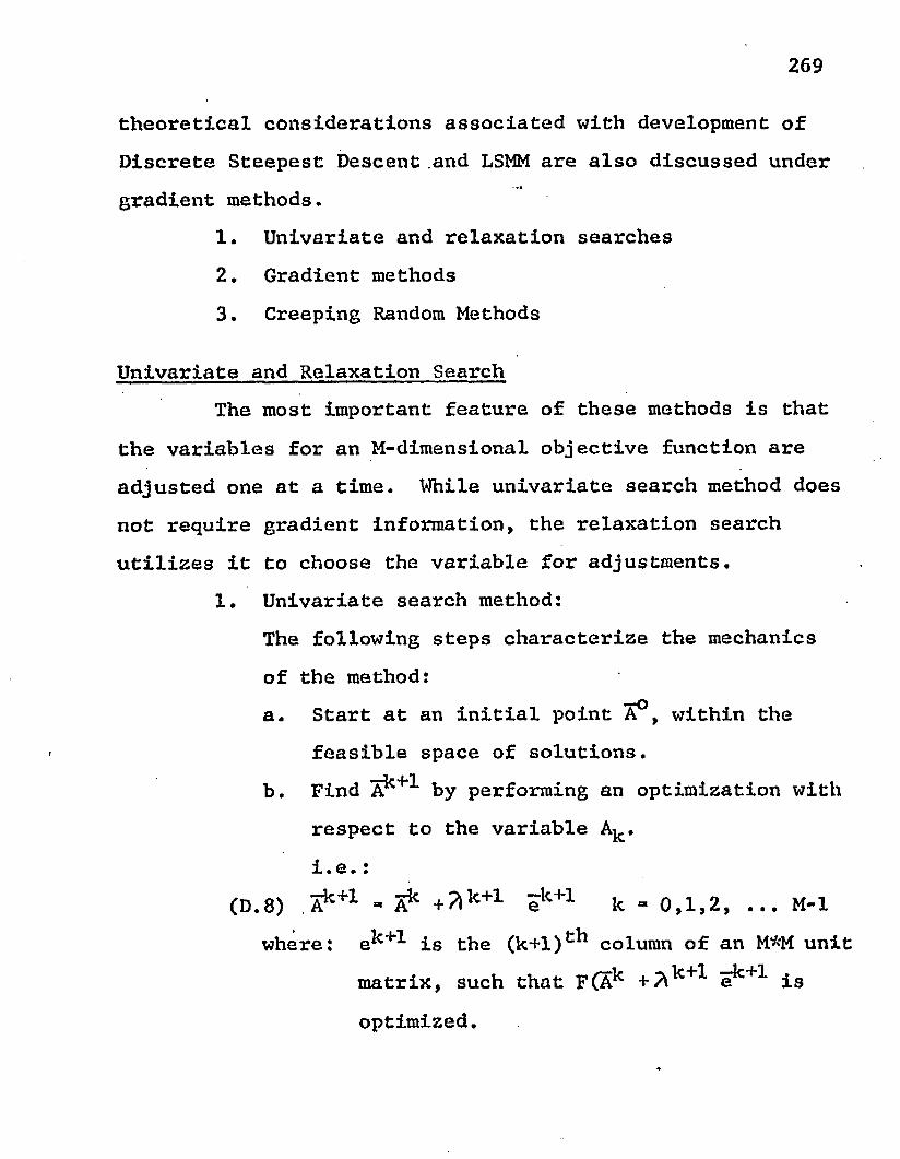
269

theoretical considerations associated with development of Discrete Steepest Descent and LSMM are also discussed under gradient methods.

1. Univariate and relaxation searches2. Gradient methods3. Creeping Random Methods

Univariate and Relaxation SearchThe most important feature of these methods is that

the variables for an M-dimensional objective function are adjusted one at a time. While univariate search method does not require gradient information, the relaxation search utilizes it to choose the variable for adjustments.

1. Univariate search method:The following steps characterize the mechanics of the method:a. Start at an initial point X°, within the

feasible space of solutions.Tpb. Find Ar by performing an optimization with

respect to the variable A^.i.e.:

(D.8) ,Ak+1 - + ^ k+1 ek+1 k « 0,1,2, ... M-lwhere: ek+^ is the (k+l)tk column of an M*M unit

matrix, such that F(Ak +7ik+ isoptimized.

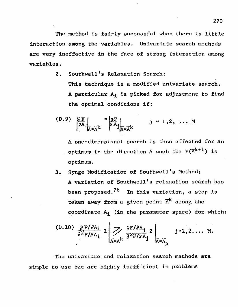
270

The method is fairly successful when there is little interaction among the variables. Univariate search methods are very ineffective in the face of strong interaction among variables.

The univariate and relaxation search methods are simple to use but are highly inefficient in problems

2. Southwell's Relaxation Search:This technique is a modified univariate search.A particular is picked for adjustment to find the optimal conditions if:

M

A one-dimensional search is then effected for an optimum in the direction A such the F(£k+1) is optimum.

3. Synge Modification of Southwell's Method:A variation of Southwell's relaxation search has been proposed.^® In this variation, a step is taken away from a given point along the coordinate A^ (in the parameter space) for which:

(D.10) j*l,2.... M.

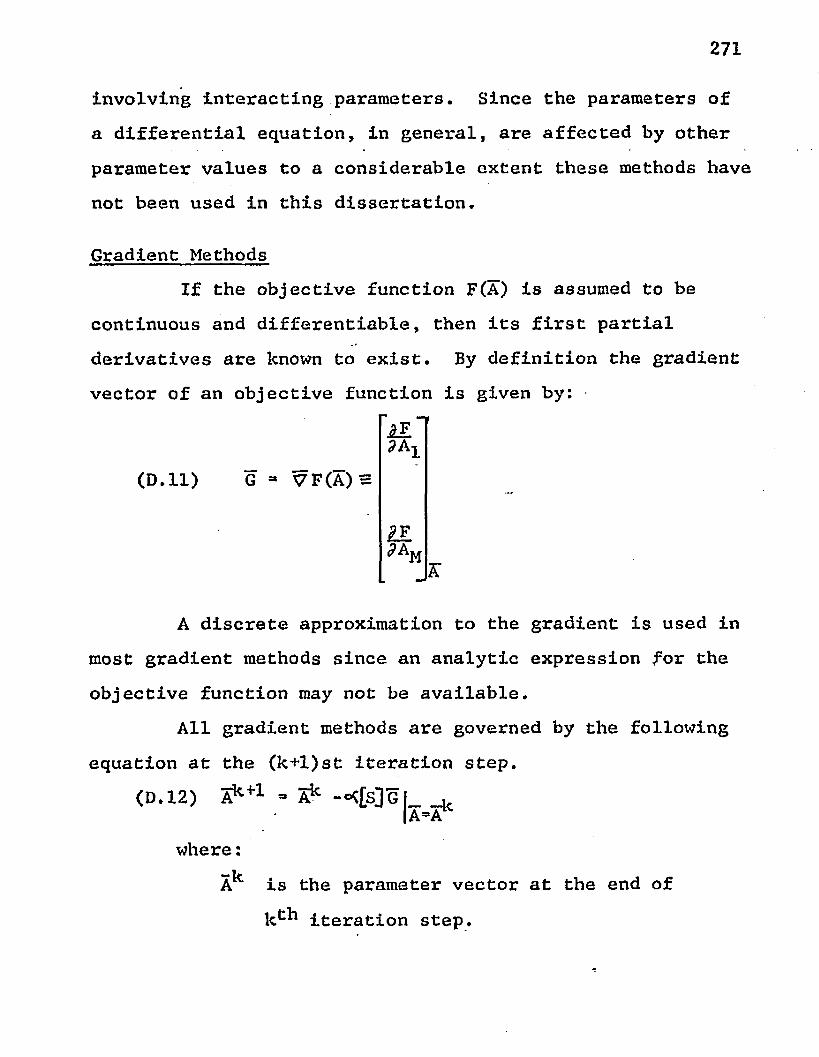
271

involving interacting parameters. Since the parameters of a differential equation, in general, are affected by other parameter values to a considerable extent these methods have not been used in this dissertation.

Gradient MethodsIf the objective function F(A) is assumed to be

continuous and differentiable, then its first partial derivatives are known to exist. By definition the gradient vector of an objective function is given by:

M i( D . l l ) 7F(A) H

ZLM MK

A discrete approximation to the gradient is used in most gradient methods since an analytic expression for the objective function may not be available.

All gradient methods are governed by the following equation at the (k+l)st iteration step.

(D .1 2 ) 5 k * 1 = -«<[s3 gA=A^

where: •rkA is the parameter vector at the end of

k*-*1 iteration step.

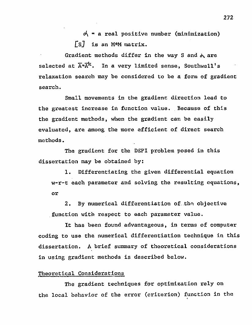
272

cf\ “ a real positive number (minimization) is] is an M*M matrix.

Gradient methods differ in the way S and ^ are selected at A^A^. In a very limited sense, Southwell's relaxation search may be considered to be a form of gradient search.

Small movements in the gradient direction lead to the greatest increase in function value. Because of this the gradient methods, when the gradient can be easily evaluated, are among the more efficient of direct search methods.

The gradient for the DEPI problem posed in this dissertation may be obtained by:

1. Differentiating the given differential equation w-r-t each parameter and solving the resulting equations, or

2. By numerical differentiation of. th^ objective function with respect to each parameter value.

It has been found advantageous, in terms of computer coding to use the numerical differentiation technique in this dissertation. A brief summary of theoretical considerations in using gradient methods is described below.

Theoretical ConsiderationsThe gradient techniques for optimization rely on

the local behavior of the error (criterion) function in the

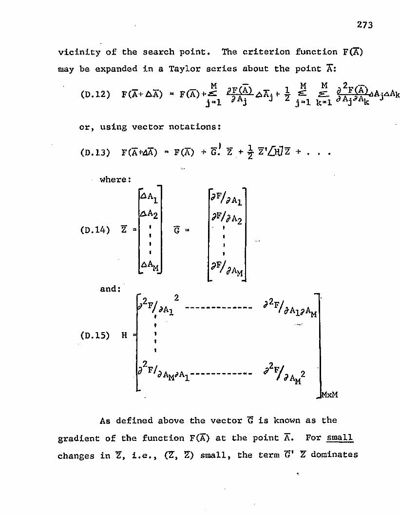
273

vicinity of the search point. The criterion function F(X) may be expanded in a Taylor series about the point T:

(D. 12) F(A+AA) - F(A)+i: ^ sLj»X ^Aj J ^ j»l k*l M jM k

or, using vector notations:

where:

(D.14) Z

* Aia.a2

t t t I

M

- F(A) + G.* Z +

3®hk2G - - i

i>

J > is

and:

M

(D.15) H

a2F/

?2f/

A / . 2H

JMxM

As defined above the vector 15 is known as the gradient of the function F(A) at the point A. For small changes in i.e., (2", 2) small, the term <5' 2 dominates

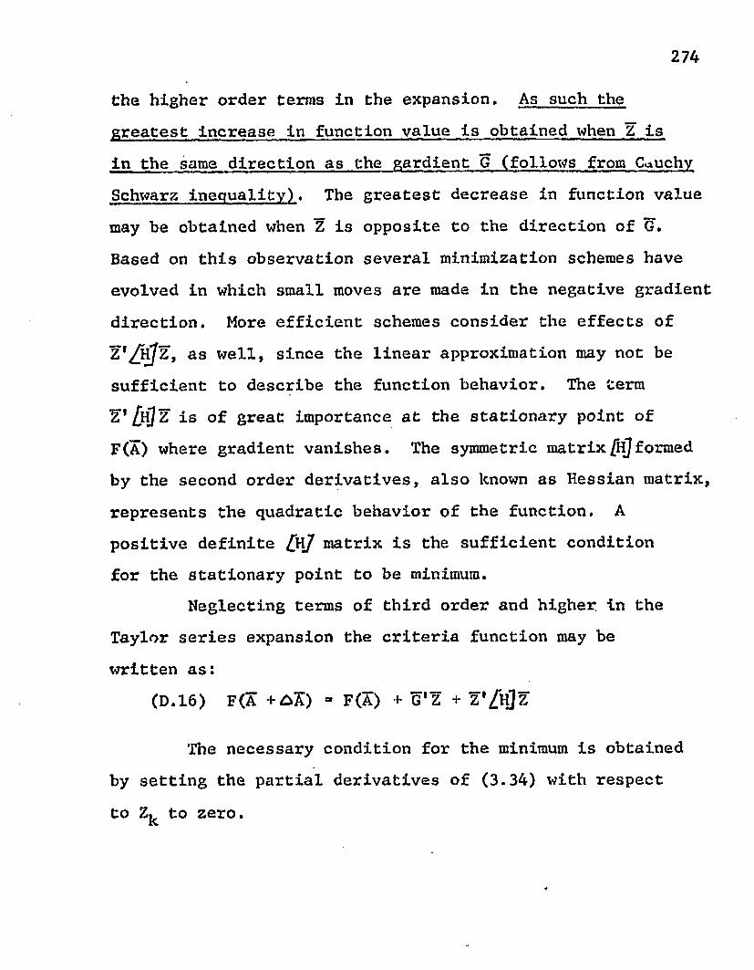
274

the higher order terras in the expansion. As such the greatest increase in function value is obtained when Z is in the same direction as the gardient G (follows from Cauchy Schwarz inequality). The greatest decrease in function value may be obtained when Z is opposite to the direction of G.Based on this observation several minimization schemes have evolved in which small moves are made in the negative gradient direction. More efficient schemes consider the effects of Vfrjz, as well, since the linear approximation may not be sufficient to describe the function behavior. The term

Z is of great importance at the stationary point of F(A) where gradient vanishes. The symmetric matrix/Hi] formed by the second order derivatives, also known as Hessian matrix, represents the quadratic behavior of the function. A positive definite IH/ matrix is the sufficient condition for the stationary point to be minimum.

Neglecting terms of third order and higher in the Taylor series expansion the criteria function may be written as:

(D.16) F(A +££) » F(£) + G'Z + Z'/Hjz

The necessary condition for the minimum is obtained by setting the partial derivatives of (3.34) with respect to Z^ to zero.

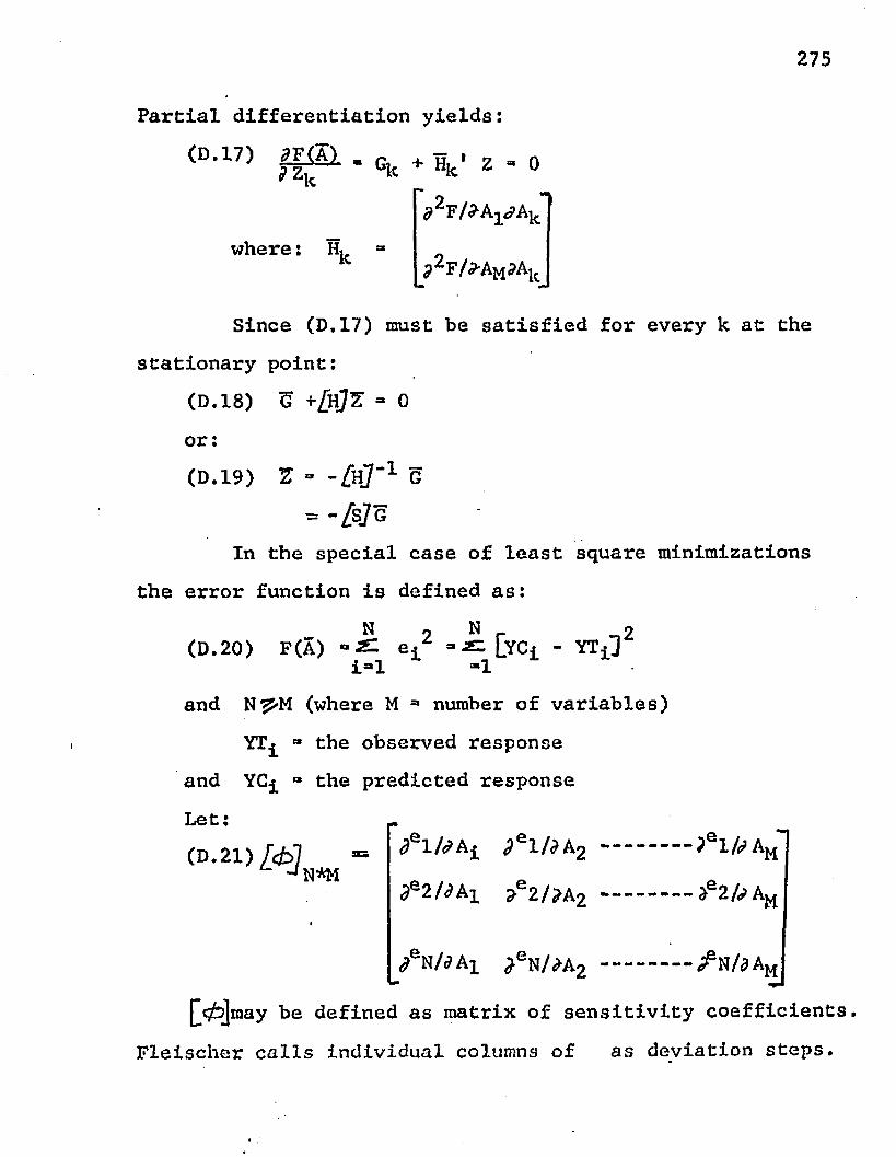
275

Partial differentiation yields:(D.17) ^ + ifk . z - o

f)^‘&F/^A1<?Akwhere: H, ?2F/^ Aj ?Ak

Since (D.17) must be satisfied for every k at the stationary point:

(D.18) <S = 0or:

f-1 k(D.19) Z - -ZkJ'-1- G= -/sJg

In the special case of least square minimizations the error function is defined as:

N ? N r -,2(D.20) F(A) e ^ =» lYCt - Y T ji=l *1

and (where M =• number of variables)YT^ “ the observed response

and YCX » the predicted response Let:(D.21) /ct>7 as 3 1 <?e l / * A 2 ----

' a <<0rv1111a

2e 2 / M x 7 2/ M 2 ----

/ n / ^ a x ^ e N / M 2 ---- ----- / n /<?a m

£c£)|may be defined as matrix of sensitivity coefficients Fleischer calls individual columns of as deviation steps.

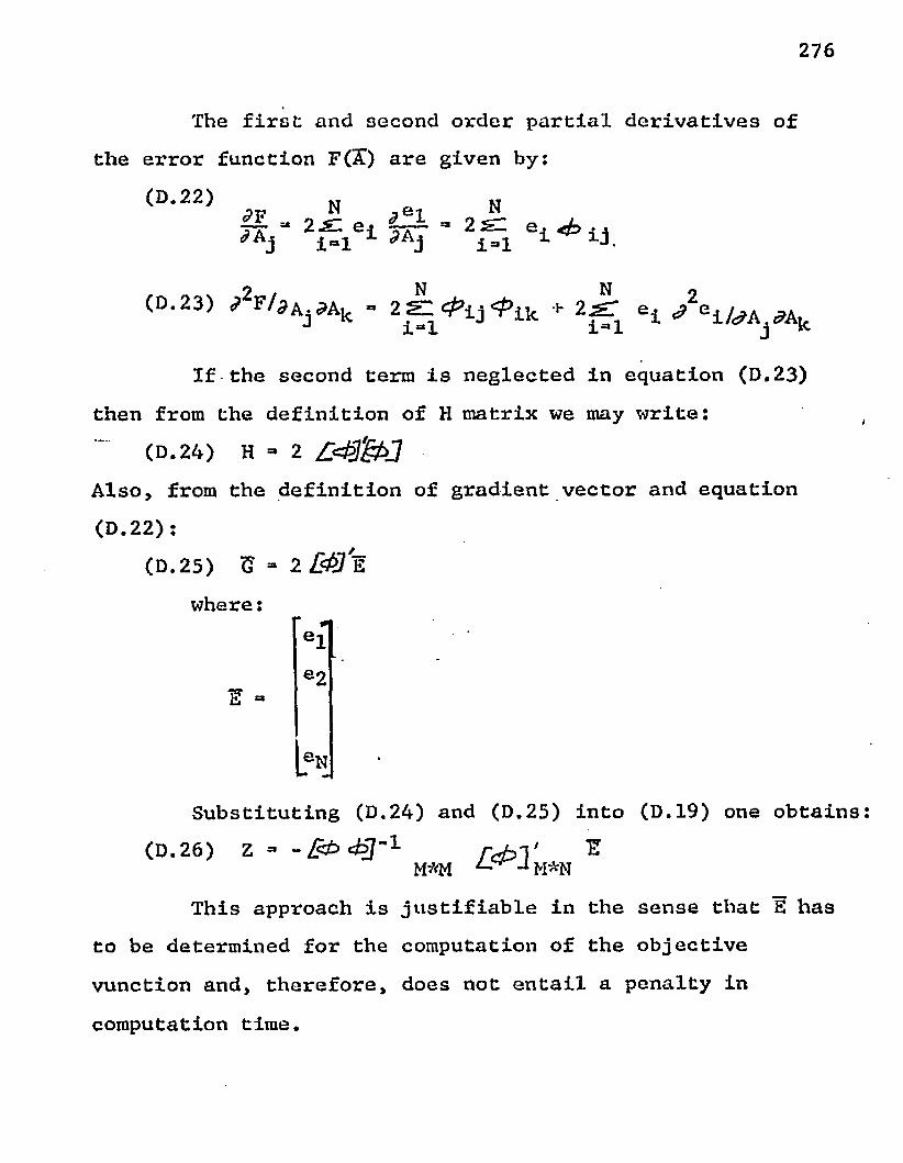
2 7 6

The first and 3econd order partial derivatives of the error function F(£) are given by:

( D ‘22) as? N a a X Nfi- - e± > 2 £ e. <t> , ±'Aj i-1 1 >Aj i=lN N(D.23) i F/5 A .^Ak - 2 2 ^ ^ * 2^T et

If the second terra is neglected in equation (D.23) then from the definition of H matrix we may write:

(D.24) H - 2 £<=@'&J Also, from the definition of gradient vector and equation (D.22):

(D.25) S » 2 &>J'e where:

r*i

E «*e2

L«hSubstituting (D.24) and (D.25) into (D.19) one obtains

(D.26) Z - -£<& / W ? V EM*M ^ J M*N

This approach is justifiable in the sense that E has to be determined for the computation of the objective vunction and, therefore, does not entail a penalty in computation time.

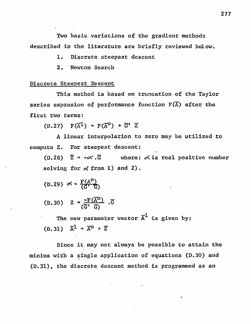
277

Two basic variations of the gradient methods described in the literature are briefly reviewed below.

1. Discrete steepest descent2. Newton Search

Discrete Steepest DescentThis method is based on truncation of the Taylor

series expansion of performance function F(A) after the first two terms:

(D.27) FCA1) - F(A°) + G* ZA linear interpolation to zero may be utilized to

compute Z. For steepest descent:(D.28) Z 3 -<?C.G where: e/\ is real positive numbersolving for of from 1) and 2).

(D. 29) 31

(D.30) Z » .G(G1 G)The new parameter vector A is given by:

(D.31) A1 - TP + Z

Since it may not always be possible to attain the minima with a single application of equations (D.30) and (D.31), the discrete descent method is programmed as an

278

iterative procedure. The equation for iteration at the (k+l)st step is given by:

(D. 32) Sk+1 = Ak - .G

Where °< is chosen according to equation (D.29) withthe additional constraint that:

(D.33) F(Ak+1)^iF(Ak)Usually a one-dimensional search along the gardient

direction is incorporated to obtain an optimum c< . Thisoptimum c< results in the lowest function value F(Ak+l) at the(k+l)th iteration step. This approach has been referred toas "Optimum Steepest D e s c e n t . I t has been subsequentlypointed out by several authors that this designation ismisleading since the gradient is strongly dependent on the

77scales of parameters. Quite often improvements in convergence can be made by incorporating features from the geometry of the objective function F(£) in parameter space. Discrete steepest descent technique has been applied to the DEPI problem with a one-dimensional search for a minimum of each iteration step.

Newton SearchThis method utilizes second partial derivative

information at each iteration step in addition to the

279k+1gradient. The new parameter vector A , at the (k+X)st

iteration step, is generated using the following equation:

(D.34) A**1 - 5^ -&}'1 &- & -^Sj5k

Since the chief drawback of the newton method is the computational effort involved in evaluation of Fletcher and Powell^ devised a method (DFP), discussed in Chapter III, which constructs a matrix at the end of M (number of parameters of the objective function) iteration steps. In case of DEPI problem the objective function has been cast in the form of sum squared error between the observed response YT and predicted model response YC. Thus, approximations to the second order derivatives are generated as part of the effort involved in computing function value and the gradient. To exploit this, a subroutine LSMM has been programmed based on equation (D.26) (Chapter III).

Creeping Random MethodsOAThese methods described by Brooks' are used to

improve the efficiency of the random method described earlier (Chapter III). The principle used is to add a bias to the random search method by favoring the searches around the current best estimates of 105. One possible way to achieve this is to shrink the size of parameter space

280

after a number of random searches around the current best estimates. The steps taken on a random search with this bias are:

1. Conduct a number of random searches in the entire region and compare the results at each step with the current best point A. Compare the final results with the function value obtained at the given starting vector and choose the best point 55.

2. Shrink the feasible region as below:A°Max “ 1*2*55 ^Arbitrarily limited to + 20%.

coefficient value)AOtfin ■* 0.8*55

3. Conduct a number (arbitrary) of searches in the region defined in step 2 and choose the best AO. If the function value is below a specified tolerance stop search. Otherwise go to step 2.

REFERENCES

1.

2.3.

4.

5.

6.

7.

8.

9.

1 0 .

Alexander, R. S. Viscoelastic determinants of musclecontractility and "cardiac tone." Fed. Froc. 21:1001, 1962.

Grodins, F. S. Control Theory and Biological Systems. Columbia University Press, 1963.

Grodins, F. S. Integrative cardiovascular physiology: a mathematical synthesis of cardiac and blood vessel hemodynamics. Quart. Rev. Biol. 34:93, 1959.

Dodge, H. T.; Sandler, H.; Baxley, W. A.; Hawley, R. R. Usefulness and limitations of radiographic methods for determining left ventricular volume. Amer. J . Cardiol. 18:10, 1966.

Robinson, A. A. Quantitative analysis of the control of cardiac output in the isolated left ventricle.Circ. Res. 17:207, 1965.

Hill, A. V. Heat of shortening and dynamic constants of muscle. Proc. Roy. Soc. London (B) 126:136, 1938-39.

Grodins, F. S. and Buoncristiani. "General Formulation of the Cardiovascular Control Problem, Mathematical Models of the Mechanical System," in Physical Bases of Circulatory Transport. Regulation and Exchange. Reeve and Guyton (ed.), W. B. Saunders, Philadelphia, 1967.

Brady, A. J. Three element model of muscle mechanics:Its applicability to cardiac muscle. Physiologist 10:75, 1967.

Sonnenblick, E. H. Series elastic and contractile elements in heart muscle: Changes in musclelength. Fed. Proc. 23:118, 1969.

Pollack, G. H. Maximum velocity as an index ofcontractility in cardiac muscle. Circ. Res. 26:111 1970.

281

282

XI. Jewel, B. R. and D. R. Wilkie. The mechanical properties of relaxing muscle. J. Physiol. 152:30, 1960.

12. Schwan, H. P. (Edited) Biological Engineering, Chapter 5 McGraw Hill Book Company7 New York, 19697

13‘. Wiener, F., Morkin, E. Skalalc, R. and Fishman, A. P.Wave propagation in the pulmonary circulation.Circ. Res. 19:834, 1966.

14. Davilla, J. C. and Sanmarco, M. E. An analysis of fitof mathematical models applicable to the measurement of left ventricular volume. Am. J. Cardiol. 18:31, 1966.

15. Rushmer, R. F. Pressure-Circumference relations ofleft ventricle. Am. J. Physiol. 186:115-121, 1956.

16. Hefner, L. L., Coghlan, H. C., Jones, W. B., and Reeves,J. J. Distensibilitv of dog ventricle. Am. J,Physiol. 201:97-101, 1961. '

17. Patterson, S. W., Piper, H., and .Starling, E. H., Theregulation of the heart beat. J. Physiol., 48:465-513, 1914.

18. Rushmer, R. F., and Thai, N. Factors influencing strokevolume: a cinefluorographic study of angiocardiography. Am. J. Physiol. 168:509-521, 1952.

19. Mitchell, J. H., Linden, R. J. and Sarnoff, S. J.Influence of cardiac sympathetic and vagal nerve stimulation on the relation between left ventricular diastolic pressure and myocardial segment length. Circulation Research, 8:1100-1107, 1960.

20. Rosenblueth, A., Alanis, J., and Rubio, R. Someproperties of the mammalian ventricular muscle.Arch. Intern. Physiol. Blochim, 67:276-293, 1959.

21. Sonnenblick, E. H. Force-velocity relations in mammalianheart muscle. Am. J. Physiol. 202:931-939, 1962.

22. Harvey, W. Anatomical Studies on the Motion of theHeart and Blood. The Leake translation (fourth ed.) Charles C. Thomas, Springfield, Illinois, U.S.A.,1958.

23.

24.

25.

26.

27.

28.

29.

30.

31.

32.

33.

34.

283Frank, 0. "The basic shape of the arterial pulse,"

Zeitschrift fur Biologie 37, 483-526, 1899,(translated by F. W. Cope in Biological and Medical Physics. 10, 282-290, 1965 (Ed.) John H. Lawrence and J. W. Gofman. Academic Press, N.Y., 1965).

Noordergraff, A.; Verdoun, P. D.; Boom, H. B. K. The Use of ah Analog Computer in a Circulation Model,Prog. Cardiov. Disease. 419, 1963.

Beneken, J. E. W. and Dewitt, B. A physical approach to hemodynamic aspects of the human cardiovascular system. In Physical Basis of Circulatory Transport (ed.) E. B. Reeve and A. C. Guyton. Philadelphia: Saunders, 1967.

Mcdonald, D. A. Blood flow in arteries. E. Arnold, London. 1960.

Rushmer, R. F. Applicability of Starling's law of the heart to intact, unanaesthetized animals. Physiol. Rev., 35:107, 1955.

Van Harreveld, A. and Shadle, 0. W. On hemodynamics, Arch. Int. Physiol. 54:165, 1951.

Snyder, M. F. and Rideout, V. C. Computer simulation studies of venous circulation, unpublished manuscript, University of Wisconsin, March, 1967.

Mcleod, J. and Defares, J. G. Analog computer simulation of heart action. AIEE Trans. 81, pp. 419-426,January, 1963. —

Attinger, E. 0. and Anne, A. Simulation of theCardiovascular system. Ann. N.Y.‘ Acad. Sci.. 128: 810-829, 1966. “ !

Sonnenblick, E. H. Implications of muscle-mechanics in the heart. Fed. Proc. 21, 975-990, 1962.

Warner, H. R. Use of analogue computers in the study of control mechanisms in the circulation, Fed.Proc., 21, 1, 1962.

Abel, F. L. An analysis of the left ventricle as a pressure and flow generator in the intact systemic circulation IEEE Trans. Blo-Med Eng. BME-13, 4, 182-188, 1966.

35.

36.

37.

38.

39.

40.

41.

42.

43.

44.

45.

284

Mcleod, J. Computer simulation of tbe( hydrodynamics of the cardiovascular system. Simulators for Circulation Research. Med. Electronics, pp. 766-795, 1965. j

Katra, J. A. and Rideout, V. C. Computer Simulation of the Human Pulmonai'y Cardiovascular system (abstract), Proc. 19th Annual Conference on Eng. in Med. Biol.,• m s : ------------------------ 12------------------

Holt, J. P. Flow of liquids through collapsible tubes, Circ. Res. 7:342-350, 1959.

Hill, A. V. Work and heart in a muscle twitch. Proc.Roy. Soc. London B, 136:220-228, 1949.

Peterson, L. H. The dynamics of pulsatile blood flow, Circ. Res. 2, 127-139, 1964.

Rushraer, R. F. Cardiovascular Dynamics, 2nd Edition,W. B. Saunders, Philadelphia, 1961.

Pieper, Heinz, P. Catheter-tip instrument for measuring left ventricular diameter in closed­chested dogs, J. Appl. Physiol., 21, 4, 1412-1415, July, 1966.

Wildenthal, K., Mullins, C. B., Harris, M. D.,Mitchell, J. H. Left Ventricular end-diastolic distnesibility after norepinephrine and propranolol. Am. J. Physiol. 217, 3, 812-818, 1969.

Tsakinis, A. G., Vandenberg, R. A., Banchero, N.Sturm, R. E., and Wood, E. H. Variations of left ventricular end-diastolic pressure^ volume, and ejection fracture with changes in outflow resistance in anesthetized intact dogs. Circ. Research, 23, .213-222, 1968. X

Monroe, R. G., LaForge, C. G., Gamble, W. J.,Rosenthal, A. and Honda, S. "Left ventricular pressure-volume relations and performance as affecged by sudden increases in developed pressure, 1 Circ. Res., 22, 333-344, 1968.

Hefner, L. L. Coghlan, H. C., Jones, W. B., and Reeves,T. J. Distensibility of the dog left ventricle,Am. J. Physiol., 201, 97-101, 1961^

46.

47.

48.

49.

50.

51.

52.

53.

54.

55.

56.

57.

285

Wildenthal, K., Mierzwiak, D. S., and Mitchell, J. H. Influence of vagal stimulation on left ventricular end-diastolic distensibilitv. Am. J. Physiol., 217,5, 1446-1450, 1969.

Adolph, R. J. Compliance of the Apex of the leftventricle in unanesthetized doKS, J. Appl. Physiol.,20, 4, 758-762, 1965.

Snyder, M. F., Rideout, V. C., and Hillestad, R. J,Computer Modeling of the Human Systemic Arterial Tree, J. Biomechanics, 1, 341-353, 1968.

Rideout, V. C. and Dick, D. E. Difference-differential equations for fluid flow in distensible tubes, IEEE trans. Bio. Med. Eng. BME-14, 171-177, 1967.

De Pater, L. and Vandenberg, J. W. An electrical analogue of the entire human circulatory system,Med. Electron. Biol. Eng., 2, 161-166, 1964.

Beneken, J. E. W. and Grupping, J. C., M. Electronic analog computer model of the human circulatory system, Medical Electronics, 770-785, 1965.

Noble, M. I. M., Milne, E. N. C., Goerke, R. J.,Carlson, E., Domenech, R. J., Saunders, K. B., and Hoffman, J. I. E. Left ventricular filling and diastolic pressure-volume relations in the concious dog. Circ. Res. 25:269-283, Feb. 1969.

Diamond, G., Forrester, J. S., Hargis, J., Parmley, W. W, Danzig, R., and Swan, H. J, C. Diastolic pressure- volume relationship in the canine left ventricle.Circ. Res., 29, 267-275, Sept, 1971.

Hamlin, R, L. Fentanyl Citrate-Droperidol and Fentobari- tal for intravenous anesthesia in dogs. J. A. V. M. A ., 152, 4, 360-364, Feb., 1968.

Zadeh, L. A. From circuit theory to system theory.Proc. IRE 50, 850-865, 1962,

Pierre, D. A. "Optimization theory with applications” John Wiley, 1969.

Wilde, D. J. "Optimum Seeking Methods,11 Englewood Cliffs, N.J.:Prentice-Hall, 1969.

58.

59.

60.

61.

62.

63.

64.

65.

66.

67.

68.

69.

70.

286Brooke, S. H. "A comparison of Maximum Seeking Methods."

Operations Research, 430-457, July-Aug., 1959.McGhee, R. B. "Some parameter optimization techniques,"

Digital Computer User's Handbook, New York: McGraw-miTTT557T------- ----------Dantzig, G. B. Linear programming and extensions,

Princeton, NTjTT Princeton University Press, 1963.Clyraer, A. B. Direct system synthesis by means of

computers, A.I.E.E. pp. 798-806, 1959.Young, P. C. The determination of parameters of a

dynamic process. The Radio and Electronic Engineer, 345-361, 1965.

«

Leitman, George (ed). Optimization Techniques with Applications to Aerospace Systems, New York:Academic Press, 1962.

Eykhoff, P. Some fundamental aspects of process parameter estimation, IEEE Trans, on Automatic Control, AC-8, 4, 347-357, October, 1963.

Bekey, G. and Maloney, A. Parameter Identification with a hybrid computer implementation of the Fletcher- Powell method. Proc. the Third International Conference on System Sciences, Part 1, pp. 175-177,vrvr.

Korn, G. A. and Korn, T. M Electronic Analog and Hybrid Computers, New York: McGraw-Hill-, 1964.

Horwitz, L. D., Bishop, V. S., Stone, H. L., andStegall, H. F. Continuous measurement of internal left ventricular diameter, J. Appl. Physiol. 24,5, 738-740, 1968.

Bishop, W. S., Horwitz, L. D., Stone, H. L., Stegall,H. F. and Engelken. Left ventricular internal diameter and cardiac function in conscious dogs,J. Appl. Physiol., 27, 5, 619-623, 1969.

Bishop, V. S. and Stone, H. L. Quantitative description of ventricular output curves in conscious dogs, Circulation Research, 20, 6, 581-586, 1967.

Kiefer, J. Sequential minimax search for a maximum,Proc. Am. Math, Soc., 4, 502^506, 1953.

71.

72.

73.

74.

75.

76.

77.

78.

79.

80.

81.

287iBekey, G. and McGhee, R. B. "Gradient Methods for the

Optimization of dynamic system parameters by hybrid computation," in Computing Method^ in Optimization Problemst Balalcrishman, A. V. and| X. W. Newstadt (ed.) New York: Academic Press, 1964.

Bellman, R. Dynamic Programming;. Princeton, N.J.: Princeton University Press, 1957.j

iPotts, T. F., Ornstein, G. N., and Clymer, A. B. The automatic determination of Human and other system parameters, Proc. Western Joint Computer Conference, pp. 645-660,W ; ------------- ----------------

iBeale, E. M. L. "Survey of Integer Programming,"

Operations Research Quarterly, 16* 219-229,June, 1965. 1

Southwell, R. V. Relaxation Methodsiin Theoretical Physics, New York: Oxford University Press, 194*6.

Synge, J. L. "A geometrical interpretation of theRelaxation Method," Quarterly of Applied Mathematics,2, 87-89, April, 194?:------------ ----------------

Brown, R. R. "A generalized Computer Procedure for the design of Optimum Systems--Parts I and XI," AIEE Transactions, Part I, Communication and Electronics,78,’"285-2937 July71959”---------- ------------------

Fletcher, R. and Powell, M. J. D. "A rapidly convergent descent method for minimization," The Computer Journal, 6, 163-168, July, 1963.

Powell, M. J. D. "An efficient method for finding the minimum of a function of several variables without calculating derivatives," The Computer Journal, 7, 149-154, July, 1964.

Fletcher, R. and Reeve, C. M. "Function minimization by coniugate gradients," The Computer Journal, 7,149-154, July, 1964.

Forsythe, G. E and Motzkin, T. S. "Acceleration of the optimum gradient method— Preliminary Report (abstract). Bulletin of the American Mathematical Society, 57, 304-305,' July,"1931“ :

28882. Shah, B. V., Buehler, R. J., and Kempthorne, 0. "Some

algorithms for minimizing a function of several variables," Journal of the Society of Industrial and Applied Mathematics, 12, 74-92,March, 1964.

83. Hooke, R, and Jeeves, T. A. "Direct Search Solutionof Numerical and Statistical problems," Journal of Association for computing Machinery, 8, 212-229, April, 1961.

84. Brooks, S. H. "A Discussion of Random Methods forSeeking Minima," Operations Research, 6, 244-251, March, 1958.

85. Eykhoff, P. and Astrora, K. J. System Identification— ASurvey, Automatica, 7, 123-162, 1971 (222 refs.).

86. Beckman, F. S. The Solution of linear equations byconjugate gradient method, Chapter 4, Mathematical Methods for Digital Computers. John Wiley, 1960.

87. Marquardt, D. W. An Algorithm for least squareestimation of nonlinear parameters, J. Soc. Indust. Appl. Math., 11, 2, 431-441, 1963.

88. Fleischer, P. E. Optimization Techniques in SystemDesign. In System Analysis by Digital Computer, pp. 175-217. (ed) Franklin, F. and James F. kaiser, John Wiley & Sons, Inc., 1966.

89. Mancini, Paolo and Pilo, Alessandro. "A Computerprogram for multiexponential fitting by the peeling method," Computers and Biomedical Research,3, 1-14, 1970.

90. Lemaitre, A. and Mallenge, J. P. An efficient methodfor raultiexponentlal fitting with a computer,Comp. Bio. Med. Res., 4, 5, 555-560, 1971.

91. Meissinger, H. F. and Bekey, G. A. "An analysis ofcontinums parameter identification method, 'Simulation, 94-102, Feb. 1966.

92. Beltrami, E. J. A Comparison of some recent iterativemethods for the numerical solution of nonlinear programs, Conference on Computing Methods in Optimization Problems. A. V. Balakrishnan (ed.),Acad. Press, New York, 1968.