UnitedStates Postgraduate School

NPS-55TW70062A

SmCAL BEFOBT BCflOiwvttFoarowwAWsaMOWTKMT. CALtfOWIIA M

United StatesNaval Postgraduate School

APPLICATION OF DIFFERENTIAL GAMES TO PROBLEMS

OF MILITARY CONFLICT:

TACTICAL ALLOCATION PROBLEMS -- PART I

by

James G. Taylor

19 June 1970

This document has been approved for public release and sale

its distribution is unlimited.

FEDDOCSD 208.14/2:NPS-55TW70062A

NAVAL POSTGRADUATE SCHOOLMonterey, California

Rear Admiral R. W. McNitt, USN R. F. RinehartSuperintendent Academic Dean

ABSTRACT

:

The mathematical theory of deterministic optimal control/differentialgames is applied to the study of some tactical allocation problems for

combat described by Lanchester-type equations of warfare. A solution pro-cedure is devised for terminal control attrition games. H. K. Weiss'

supporting weapon system game is solved and several extensions considered.A sequence of one-sided dynamic allocation problems is considered to studythe dependence of optimal allocation policies upon model form. The solu-tion is developed for variable coefficient Lanchester-type equations whenthe ratio of attrition rates is constant. Several versions of Bellman'scontinuous stochastic gold-mining problem are solved by the Pontryaginmaximum principle, and their relationship to the attrition problems is

discussed. A new dynamic kill potential is developed. Several problemsfrom continuous review deterministic inventory theory are solved by the

maximum principle.

This task was supported by The Office of Naval Research.

TABLE OF CONTENTS

Section Page

I. Introduction 4

a. Optimal Control/Differential Games •>

b. Dynamic Programming

c. Tactical Allocation Problems

II. Review of Pertinent Literature

III. Some Tactical Allocation Problems

a. The Allocation Problems

b. Extensions of Lanchester-Type Models of Warfare

c. Other Topics Not Included in this Report ^

'

IV. Conclusions and Future Extensions

6

7

9

12

12

16

20

Appendix

A. The Isbell-Marlow Fire Programming Problem 22

B. H. K. Weiss' Supporting Weapon System Game 39

O -]

C. Some One-Sided Dynamic Allocation Problems ox

D. Solution to Variable Coefficient Lanchester-Type Equations 117

E. Connection with Bellman's Stochastic Gold-Mining Problem 124

F. A New Dynamic Kill Potential 16Q

G. Applications to Deterministic Inventory Theory ]_7q

n

INTRODUCTION .

This report documents research findings for the time period 30

March 1970 to 19 June 1970 under support of NR 276-027. This report

discusses applications of the theory of differential games to tactical

allocation problems in the Lanchester theory of combat. We also discuss

some extensions for Lanchester-type models of warfare and deterministic

inventory theory. A companion report [76] discusses other research

findings of the contract period with respect to surveillance-evasion

problems of Naval warfare.

The goal of this research is to determine the structure of optimal

allocation policies for tactical situations describable by Lanchester-

type equations of warfare. We hope to provide insight into such questions

as

(1) How should targets be selected?

(2) Do target priorities change with time?

(3) Do battle termination circumstances effect the optimalallocation policies?

(4) How does the nature of the attrition process effect targetselection?

(5) What is the effect of ammunition constraints?

(6) How does the uncertainty and confusion of combat effect the

optimal selection rules?

We develop our theory of target selection through the examination of a

sequence of simplified models. These combat models are too simple to

be taken literally but should be interpreted as indicating general

principles to serve as hypotheses for subsequent computer simulation

studies or field experimentation.

In warfare decisions must be made sequentially over a period of

time, and the world is changed as a result of these decisions. The

Lanchester theory of combat has been developed to describe such dynamic

situations. Of even more interest to defense planners than how to

describe combat, is how to optimize the dynamics of combat. Many times

the static optimization techniques of linear and non-linear programming

are not applicable, so new dynamic optimization techniques were developed

in the 1950's.

Actually, many such situations may be formulated as classical con-

strained calculus of variations problems (technically referred to as

the problems of Bolza, Lagrange and Mayer). Because of inequality

constraints and non-negative variables in such problems, the classical

methods are difficult to apply. Thus, dynamic programming [9] was

originally developed as a computational technique for variational pro-

blems, although its principles have proven to be of much wider applica-

bility. This was also the impetus for the development of the maximum

principle by the Soviet mathematician L. Pontryagin [68] . During this

period military problems also rekindled interest in the game theory of

J. von Neumann [78] with extensions being made to multi-move discrete

games [9], [29] and differential games [50]. It seems appropriate to

ciscuss these techniques briefly.

a. Optimal Control/Differential Games .

These techniques may be used to optimize systems whose behavior

is described by a system of differential equations. The same basic

concepts are referred to as optimal control when there is one controller

and one criterion function and as a differential game with two controllers

and two criterion functions (which sum to zero). Recently the term

"generalized control theory" has been coined [42], [43] for these dynamic

optimization techniques. A common point of such models is that time

is treated continuously. Major work has been done by L. Pontryagin

and others in the USSR (see survey papers by [13], [71] and references

in [8], [33]), and R. Bellman, L. Berkovitz, Y. C. Ho, and others in

the US. R. Issacs has independently developed an extensive theory

of differential games and has published a book containing numerous

examples [50]

.

However, these techniques apply primarily to deterministic systems.

Frequently numerical methods must be used when closed-form analytic

solutions can't be obtained. Dynamic programming was developed at RAND

by R. Bellman and others [9], [10] for such cases.

b . Dynamic Programming .

Although numerical solution of variational problems was one of

the initial reasons for the development of dynamic programming, this

technique has proven to be of much wider applicability. It is a dual

approach to Lagrange's method of variations, which treats an extremal

curve as a sequence of points and develops a differential equation to

be satisfied at each such point. On the other hand, dynamic programming

generates an optimal trajectory by considering the "direction of best

return" working backwards from the problem's end. It bears a close

relationship to C. Caratheodory' s notion of a geodesic gradient, and

this has rekindled interest in much classical work.

Although we haven't explicitly used dynamic programming in the

present work, its underlying principle of optimality [9] continues to

apply when the assumption required by differential game theory of con-

tinuous time no longer holds. Historically (see Chapter X of [9]),

multi-move discrete games were considered before differential games,

which are a limiting case. For future work in which it may be desirable

to closer approximate the real world with less restrictive assumptions

(for example, attrition rates which don't lead to closed-form solutions

of the corresponding differential equations), it may be necessary to

employ numerical procedures, and we have given this consideration.

c. Tactical Allocation Problems .

We think that combining Lanchester-type models of warfare with

the theory of differential games/dynamic programming has a great potential

for providing insight into the optimization of the dynamics of combat

continuing over a period of time with a choice of tactics available to

both sides and subject to change with time. In the present work our

goal is to determine the factors upon which the optimal allocation

depends and also what this dependence is. We have considered the follow-

ing aspects

(1) combatant objectives (form of criterion function and valuationof surviving forces)

,

(2) termination conditions of conflict,

(3) type of attrition process,

(4) force strengths,

(5) effect of resource constraints.

Our conclusion is that any or all of the above factors may influence

the structure of the optimal allocation policies depending upon the form

of the model used. Judgment is required, then, to decide which type of

model is most applicable for any specific problem.

Besides the study of problems of land combat, these models have

numerous applications to problems of Naval warfare:

(1) optimal allocation of Naval fire support,

(2) allocation of Naval airpower between ground-support andstrategic targets,

(3) worth of Naval transport capability for troop build-up incombat zone.

We envision these idealized models as being used to provide insight and

to generate hypotheses to be tested in subsequent work under less re-

strictive assumptions (such as computer Monte Carlo simulation or actual

field experimentation).

Our research approach has been to consider a sequence of models

of increasing complexity. We have considered models for two types of

choice situations

(1) selection of target type,

(2) regulation of firing rate.

We have also found it necessary to develop several extensions to the

theory of Lanchester-type models of warfare and also to differential

game theory.

In considering more and more complex models, we have started with

one-sided models and done some work for the two-sided case. We have

learned about the structure of optimal allocation policies by solving

numerous specific problems. We have found that the application of

existing theory to the prescribed duration battle is straightforward

but that (even for the one-sided case) new approaches and concepts had

to be developed for battles which terminate by the course of combat

being steered to a prescribed state. In these terminal control problems

we have considered a "fight to the finish" for mathematical convenience,

and our approach, of course, applies to any terminal control game. Our

work shows that selection of the appropriate scenario (prescribed dura-

tion or terminal control) may be an important decision in a defense

planning study. We have also applied the existing theory of differential

games to pursuit and evasion problems [76]. We have found that there

are numerous mathematical differences between pursuit-evasion and attri-

tion differential games.

These models consider the continual allocation of resources after

the battle has started. We could consider models for the initiation

and termination of conflict and also the allocation of resources across

a broad front before the actual battle begins. Such considerations are

beyond the scope of the present work.

We have also looked for other areas of interest to defense planners

for the application of the knowledge we have gained through our study

of tactical allocation problems. Thus, we consider some models of

deterministic, continuous-review inventory processes in Appendix G.

II. REVIEW OF PERTINENT LITERATURE .

We reviewed the literature in two subject areas: Lanchester theory

of combat and differential games. We do not attempt an exhaustive review

of the literature, since that was not the purpose of this research.

However, we try to highlight some major works.

One of the earliest attempts to establish a mathematical model

of the dynamics of mass combat was by Lanchester [61] in 1916. He devel-

oped several deterministic models that were a system of ordinary

differential equations which related the strengths of opposing military

10

forces to length of combat. During World War II B. 0. Koopman extended

Lanchester's results and also suggested a reformulation of the problem

in stochastic form [66]. After World War II the RAND Corporation carried

on further studies whose results were summarized by Snow [72]. H. K.

Weiss then at Aberdeen Proving Ground and others [7], [22], [28], [37], [38],

[80] , [81] have subsequently developed deterministic Lanchester models.

R. Brown developed models for the stochastic analysis of combat [23].

The relationship between the above mentioned stochastic and deterministic

Lanchester formulations was pointed out relatively early in their devel-

opment (see [72], for example) but is probably best presented in a

recent report by B. 0. Koopman [60]. Bonder [21] has done work on the

estimation of the Lanchester attrition-rate coefficient (for weapon

systems that adjust fire based on results of the previous round fired).

A good review of the Lanchester theory of combat is by Dolansky [28],

and this includes a comprehensive list of references through 1964.

The study differential games was initiated by R. Isaccs at RAND

in the early 1950's [46], [47], [48], [49], but this work has not been

available to a wide audience until quite recently [50] . His basic con-

cept, "the tenet of transition," is a generalization of Bellman's [9]

"principal of optimality" to a competitive environment, and this is used

to develop necessary conditions for optimal strategies. A more recent

and more rigorous development of these basic necessary conditions is by

Berkovitz [12]. Since the excellent paper by Ho, Bryson and Baron [44]

in 1965, there has been a literal explosion of papers on differential

games but almost all deal exclusively with pursuit-evasion problems.

Excellent survey papers which bear this out are by Simakova (Russian

11

literature) [71] and Berkovltz [13]. A more detailed review of differ-

ential game literature for pursuit and evasion applications is to be

found in a companion report [76]. At a fairly recent workshop on

differential games it was noted that there have been no new significant

examples [25] since the publication of Isaacs' book. Other books which

treat differential games are by Blaquiere et al. [16] (extension of

their geometrical approach to optimal control) and Bryson and Ho [24]

(Chapter 9)

.

In 1964 Dolansky [28] noted that the Lanchester theory of combat

was insufficiently developed in the area of target selection for combat

between heterogeneous forces (optimal control/differential games). Even

the two references cited by him, Weiss [82] and Isbell and Marlow [52],

have been subsequently extended [74]. Since Dolansky 's article, no

further examples have been published in the literature except for the

ones in Isaacs book [50].

One aspect that has impressed this author has been the diversity

of approaches applied to the same problem by the researchers at RAND.

Discrete and continuous models, deterministic and stochastic models are

used in a complementary manner to help each other and provide insight.

We note in this connection the discrete and continuous versions of the

strategic bombing problem (Bellman's stochastic gold-mining problem [9]).

We also note that the War of Attrition and Attack of Isaacs is the con-

tinuous version of other discrete sequential decision-making models of

the strategic/tactical deployment of airpower studied at RAND [14], [15],

[34].

12

Differential game theory has also been used to study target

selection in combat described by Lanchester-type equations at the

University of Michigan. Results are summarized in a report [73], which

references working papers for further details. We have not yet reviewed

these working papers. However, it appears that this work does not

consider the various possible model forms that we do in the present

work and, hence, the dependence of optimal allocation policies on model

form is not recognized.

III. SOME TACTICAL ALLOCATION PROBLEMS .

In this section we summarize results for the problems we have

studied and explain why these problems were studied. A more detailed

discussion on many points is to be found in the appendices. The current

phase of this work has stressed extension of results in the literature.

This has been by necessity both to familiarize ourselves with past

work and to extend many partial or incomplete results. The present

state of differential game/optimal control theory allows problems,

which twenty years ago would be very difficult (if not impossible) to

solve by classical variational methods, to be readily solved.

First we review the various tactical allocation problems which

we have studied, and then we discuss two extensions we have made to the

Lanchester theory of combat. A section is included to summarize some

work not included because of its incomplete nature in this report.

a. The Allocation Problems .

In Appendix A we derive a complete solution to the Isbell and

Marlow [52] fire programming problem. This is a terminal control problem

13

(the battle terminates when the course of battle has reached some

specified state) and such attrition games are not treated in Isaacs'

book [50]. We first solved this problem to gain insight into a solution

phenomenon of H. K. Weiss' supporting weapon system game [82]. In an

optimal control problem one determines extremals and domains of con-

trollability for each terminal state, but in a differential game further

investigations are required to verify that one's opponent can't "block"

entry to an unfavorable (losing) terminal state against one's extremal

strategy. It may be that he can steer the course of battle to an end

favorable (winning) to him by use of other than his extremal strategy.

This phenomenon has not occurred in any pursuit and evasion differential

game in the literature. We discuss the structure of optimal target

engagement policies for the Isbell-Marlow problem. Later (in Appendix

C) we contrast the same combat model in scenarios of a prescribed dura-

tion battle and a "fight to the finish."

In Appendix B we apply the theory of differential games to H. K.

Weiss' supporting weapon system game. This problem was originally

solved by assuming a special form for the solution [82]. Subsequent

work [58] has considered the simpler case of a prescribed duration

engagement. We have found the existing framework of differential game

theory inadequate for solving the supporting weapon system game and have

consequently introduced the concept of a "blockable" terminal state

which we have discussed briefly above. Such behavior does not occur

in a one-sided problem. The book by Blaquiere et al [16] defines a

similar concept of a "strongly playable strategy," but there are no

concrete examples given to motivate this notion.

14

In the future we would propose to formalize the notion of a

"blockable" terminal state as a contribution to the theory of differen-

tial games. We also discuss several extensions of the original support-

ing weapon system game in Appendix B. It seems appropriate to devise

further extensions to study facets like: (a) target priorities for

fire support systems, (b) when to engage enemy fire support system

instead of fire support for other forces. We have examined some scenarios

not included in this report.

In Appendix C we examine a sequence of problems to study the

dependence of optimal allocation policies on model form. We consider

two types of choice problems: (1) target selection and (2) firing rate.

In studying the problem of target selection we re-study the Isbell-

Marlow fire programming problem to learn about the structure of best

policies through a series of contrasts

(a) prescribed duration versus terminal control battle,

(b) two versus many target types,

(c) square law versus linear law attrition.

We discuss differences in the structure of optimal policies for all

these cases. We also find out such things as that if one assigns a

worth to targets in proportion to their kill rate against you, then

there is never a switch in target priorities. We also are motivated

to define the new dynamic kill potential of Appendix F.

We also study the best firing rate in a sequence of models all

having resource constraints. We are interested in ascertaining under

what circumstances does one "hold his fire." We consider a simplified

model for combat between two homogeneous forces in which one side has

15

an ammunition constraint that will be binding in a battle of prescribed

duration and the attrition rates are constant. Under these circum-

stances, the best policy is to fire at one's maximum possible rate until

all ammunition has been expended. We see that this model is not too

realistic and are led to consider cases where the attrition rates vary

with time or force separation. This leads to variable coefficient

Lanchester-type equations and has been our impetus for seeking solution

methods for such equations. We have, by necessity, had to extend the

existing theory of Lanchester-type models, and we discuss this in

another appendix (D). We also consider several other scenarios for

limited resources.

In Appendix C we have also included a discussion of the usefulness

of one-sided models for studying two-sided phenomena. We point out the

close relationship between optimal control and differential game theory.

Since the Hamiltonian is usually separable in the control variables,

i.e., a function independent of tj) + a function independent of \\t (for

a practical example where this isn't true see [ll])>we essentially have

two "independent" optimal control problems (one a maximization and the

other a minimization) and the optimal strategies are pure. We note that

this is not true for many important models in game theory (Col. Blotto

game, for example [29]).

We also discuss the implications of the idealized models we have

considered. Hence, we discuss optimal tactical allocation, intelligence,

command and control systems, and human decision making. We have learned

that optimal strategies are a function of model form, and there usually

will be several possible forms available.

16

In Appendix E we develop the solution to the continuous version

of Bellman's stochastic gold-mining (strategic bombing) problem [9] by

optimal control theory. We do so because the solution to this problem

has a very similar structure to that for allocation of fire over targets

undergoing linear law attrition. We consider two types of models: (1)

maximum return for prescribed duration use and (2) maximum return for

specified risk. The structures of the optimal allocation policies are

slightly different in these two cases. Originally, Bellman used varia-

tional methods and knowledge of discrete analogues to solve these problems,

The new methods are easier to apply and provide more insight (for example,

the distinction between the two problems considered above) . Our study

of this problem and its similarity to other tactical allocation problems

studied in Appendix C suggest that there may be a general structure

underlying all such problems. We also are motivated to consider other

formulations (for example, a force is only subject to attrition from

targets that it engages) of tactical allocation problems with Lanchester-

type models of warfare.

b. Extensions of Lanchester-Type Models of Warfare .

We have, by necessity, made two extensions to the Lanchester theory

of combat:

(1) solution to Lanchester-type equations with variable coeffi-

cients,

(2) development of notion of a dynamic kill potential.

In Appendix D we show how to solve Lanchester-type equations for combat

between two homogeneous forces when the attrition rates are variable

provided that their quotient is a constant. Solutions are developed

17

for either time or force separation as the independent variable. We

also discuss the relationship of our work to that of others [20], [73].

In Appendix F we define the concept of a weapon system firepower

potential. We obtained our motivation for this development from our

study of tactical allocation problems using optimal control theory.

Our approach provides a measure of the firepower capability of a weapon

system giving consideration to the dynamics of combat.

When one interprets the maximum principle and dual variables

which one is using (or attempts derivations) , one sees that the rate

of return for engaging a target (as measured by the rate of change of

a terminal payoff for the scenario) changes during the course of battle.

One is tempted to try to extend the notion of evolution of target worth

to cases where there is no allocation problem. By use of the adjoint

system to the Lanchester-type equations, one can do this. Our method

may be used to study such facets of combat as the worth of mobility in

battle, the effect of different range capabilities for weapon systems.

This is the end of our guided tour of the appendices.

c. Other Topics Not Included in This Report .

It seems appropriate to note two other areas of work that for one

reason or another have not been included in this report: (1) other

tactical allocation formulations and (2) target coverage problems. We

have done initial work on the formulation of other tactical allocation

formulations and (2) target coverage problems. We have done initial

work on the formulation of other tactical allocation situations

(a) fire support of several ground units,

(b) weapon system only subject to attrition when engaging a target

type.

We also did some work on coverage problems. We obtained a new

result for the hit probability against a circular target when the dis-

tribution of impact points follows an offset circular bivariate normal

distribution. Although this type of problem has been extensively studied

(in a recent survey article Eckler [31] gives 60 references; see also

Grubbs' [36] brief survey), we have discovered a new representation for

the hit probability, and this yields several useful approximations.

Consider a circular target with radius a located at the center

of an x-y rectangular coordinate system. Assume that the distribu-

tion of impact points follows an offset circular bivariate normal distri-

bution. We let

a = a = a be standard deviation of impact points,x y

y ,u be average of impact distribution,x y

and R = /\l2~+~Ht .

x y

Then

for R < a

oo ^

P = 1 - exp{-(a2 + R2)/(2o*)}. I (f) ijff),k=0

where I,(Z) is the Bessel function with imaginary argument of the firstK.

kind, of order k. It may be defined as

'Z^2m+k*2 J

Ik(Z)

^ n m!(m + k)! '

m=U

19

Also

for R > a

oo k

Phit

= exP{"^ 2 + R2 )/(2a 2)} I (§) I

k@k=l

The above formulas are readily proven through an intermediate result

of Gilliland [35]. We may also express the above in closed form through

the use of Lommel's functions of two variables (see Watson [79] p. 537).

for R < a

phit

= 1 + exP f -< a2 + R 2 )/(2o 2 )»iU1{i |z-,i

S|)

and

for R > a

Phit

= "exP^(a2 + R 2 )/(2a 2 )}{iU1

(i ^-,1J|)

+ Uj-2-,l -2-)} ,

where i = /-l and U (w,z) is Lommel's function of two variablesn

defined by

00 n+2mU (w,z) =

I (-I)"1© J («).

n ^_ ^z n+zmm=0

20

Unfortunately, there exist no tabulations for Lommel's function of two

imaginary arguments. Since several problems of physical significance

also lead to this type of solution, the creation of such tables seems

warranted.

IV. CONCLUSIONS AND FUTURE EXTENSIONS .

Here we summarize what we have done, state some generalizations,

and suggest some possible future research. Further amplification of

results and conclusions is to be found in the appendices. We have

considered the optimization of dynamic systems using the theory of

optimal control/differential games. Specifically, we have accomplished

the following:

(1) devised method for solving terminal control attrition games,

(2) compared sequence of idealized scenarios to study dependenceof optimal allocation policies on model form,

(3) developed solution to Lanchester-type equations with variablecoefficients under special circumstances,

(4) developed a new dynamic kill potential,

(5) generalized results in continuous review deterministicinventory theory (optimal inventory policies for linearproduction costs and effect of budget constraints).

Based on our studies we conclude that

(1) tactics of target selection are dependent on model form and

may be sensitive to force strengths, target acquisitionprocesses, attrition processes, and/or termination conditions

of combat,

(2) tactics for target selection depend upon "command efficiency,"

(3) for a continuous review deterministic inventory process, whenproduction costs are linear, then the optimal inventory policy

is essentially independent of the nature of holding costs

except for sometimes operating at the minimum of the shortage/

holding cost curve.

21

We suggest the following as possible future work:

(1) develop in a more mathematical fashion our theory of terminalcontrol attrition games (The examples we have solved suggestseveral necessary extensions to the existing mathematicaltheory. )

,

(2) study extensions of supporting weapon system game (We wouldexamine optimal tactics for various battle termination con-ditions and attrition processes.))

(3) further study problem of best firing rate when there areammunition constraints with either time-varying or range-varying attrition rates (This would extend models consideredin Appendix C and would use our results developed in AppendixD.),

(4) formulate allocation of forces before the inception of combatproblem (It is of interest whether the optimal strategy is

mixed for then the element of surprise becomes important in

planning a successful attack.),

(5) develop other models of tactical interest and study otherextensions in the literature (We would continue to stressthe study of the dependence of optimal tactics on model form.)

22

APPENDIX A. The Isbell-Marlow Fire Programming Problem.

In this appendix we develop a complete solution to the Isbell

and Marlow fire programming problem [52]. This is the simplest example

of more general tactical allocation problems which are terminated by

the system being steered to a specified terminal state. Subsequent

work [82] which considered the work of Isbell and Marlow has been

heuristic (not using the usual (today's) necessary conditions [12])

possibly because of the incompleteness of this prior work. We origin-

ally solved this (the Isbell-Marlow fire programming problem) in order

to gain insight into the supporting weapon system game of H. Weiss [82],

In studying simplified models of dynamic tactical allocation pro-

blems it is important to understand the dependence of the structure of

optimal policies on model form. We have discovered in our researches

that the optimal allocation policies may depend on the scenario chosen

to study the problem.

In this appendix we first state fire programming problem before«

we outline our new solution procedure and indicate its extension to two-

sided problems (differential games). Next we present the details of

the solution, after which we discuss the structure of the optimal allo-

cation policies. In view of the close connection [12], [41] between

optimal control and differential games (Isaacs), the terminology of

these two fields is used somewhat interchangeably. We begin by review-

ing previous work briefly.

An underdeveloped area [28] of the Lanchester theory of combat

is target selection for combat among heterogeneous forces. This type

23

of problem has been studied by Isbell and Marlow, who considered both

a truncated stochastic (Lanchester) process by game theoretic means [51]

and a terminal control (one-sided) differential game [52]. An attrition

differential game is an idealized combat situation described by Lanchester-

type equations over a period of time with choices of tactics available

to both sides and subject to change with time. Terminal control attri-

tion games only end when the course of combat has been steered to a

prescribed state.

In developing a theory of target selection it is important to

understand the dependence of allocation rules on the type of model chosen.

Tactical allocation problems may be studied in two types of scenarios:

(1) the prescribed duration battle and (2) the terminal control battle

(a particular case of which is the "fight to the finish"). All the

attrition examples in Isaacs' book [50] are of the first type (his "War

of Attrition and Attack" is the continuous version of the tactical air

war game [14], [15], [34] studied at RAND). Only Isbell and Marlow [52]

and Weiss [82] have studied the terminal control problem. Unfortunately,

Isbell and Marlow did not obtain a complete solution to their problem.

They could not determine when certain terminal states of combat were

reached. Weiss studied a problem which may be considered to be a general-

ization (two-sided version) of their problem. His solution procedure [82]

was a heuristic one, not involving the usual (today's) necessary condi-

tions [12], possibly because the simpler problem which he referenced

in his paper had not been completely solved.

24

a. Statement of the Problem .

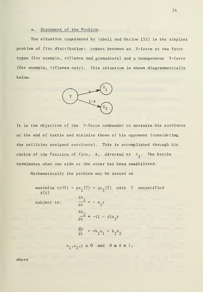
The situation considered by Isbell and Marlow [52] is the simplest

problem of fire distribution: combat between an X-force at two force

types (for example, riflemen and grenadiers) and a homogeneous Y-force

(for example, riflemen only). This situation is shown diagrammatically

below.

It is the objective of the Y-force commander to maximize his survivors

at the end of battle and minimize those of his opponent (considering

the utilities assigned survivors). This is accomplished through his

choice of the fraction of fire,<J> , directed at X-. . The battle

terminates when one side or the other has been annihilated.

Mathematically the problem may be stated as

maximize ry(T) - px (T) - qx (T) with T unspecified(t)

L

dXi

subiect to: -— = - a n ydt 1

dx" = -(1 - <j>)a„y

dtv T/

2

^ = "Vl ' b2X2

x ,x ,y ^ and £ <J> £ 1,

where

25

p, q and r are utilities assigned to surviving forces,

x1

, x and y are average force strengths,

a.. , a_ , b.. and b?

are constant attrition rates,

<J>is fraction of Y-f ire directed at x ,

and with terminal states defined by (1) x (T) = x (T) = and

(2) y(T) = 0.

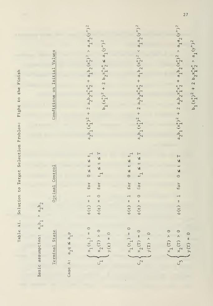
The terminal surface of the "realistic" (one-sided) game is seen

to consist of five parts:

Cx

: X;L (T) = 0, x2(T) > 0, y(T) = 0,

C2

: x (T) = before x (T) = 0, y(T) > 0,

C3

: x (T) = after x (T) = 0, y(T) > 0,

C4

: Xl (T) > 0, x2(T) = 0, y(T) = 0,

C5

: Xl (T) > 0, x2(T) > 0, y(T) = 0.

b. Solution Procedure and Extensions .

Extremal paths (a path on which the necessary conditions for

optimality are almost everywhere satisfied) may be obtained by routine

application of Pontryagin's maximum principle [68] (the original authors

used equivalent conditions independently developed by Isaacs [48]). How-

ever, in a terminal control problem we would like to know the domain of

controllability [32] for each terminal state so that tactics are deter-

mined in terms of the initial conditions of combat (and also possibly

time). We define the domain of controllability for a given terminal

26

state to be that subset of the initial state space from which extremals

lead to the terminal state.

The following procedure has been used to solve the above problem:

(a) extremal control is determined by maximizing the Hamiltonian;

since the state variables (force strengths) are non-negative, the

control depends, in many cases, only on relationships between the

dual variables (marginal return from destroying target),

(b) from each separate terminal state, the time history of the dual

variables is obtained by a backward integration of the adjoint

system of differential equations; for a square law attrition

process, the adjoint equations are independent of the state

variables

,

(c) for each terminal state the domain of controllability is deter-

mined by forward integration of the state equations using the

time history of extremal control developed in (b) ; changes in

control with time (existence of transition surface) may have to

be considered in this step.

It is noted that Isbell and Marlow [52] stopped at step (b) above.

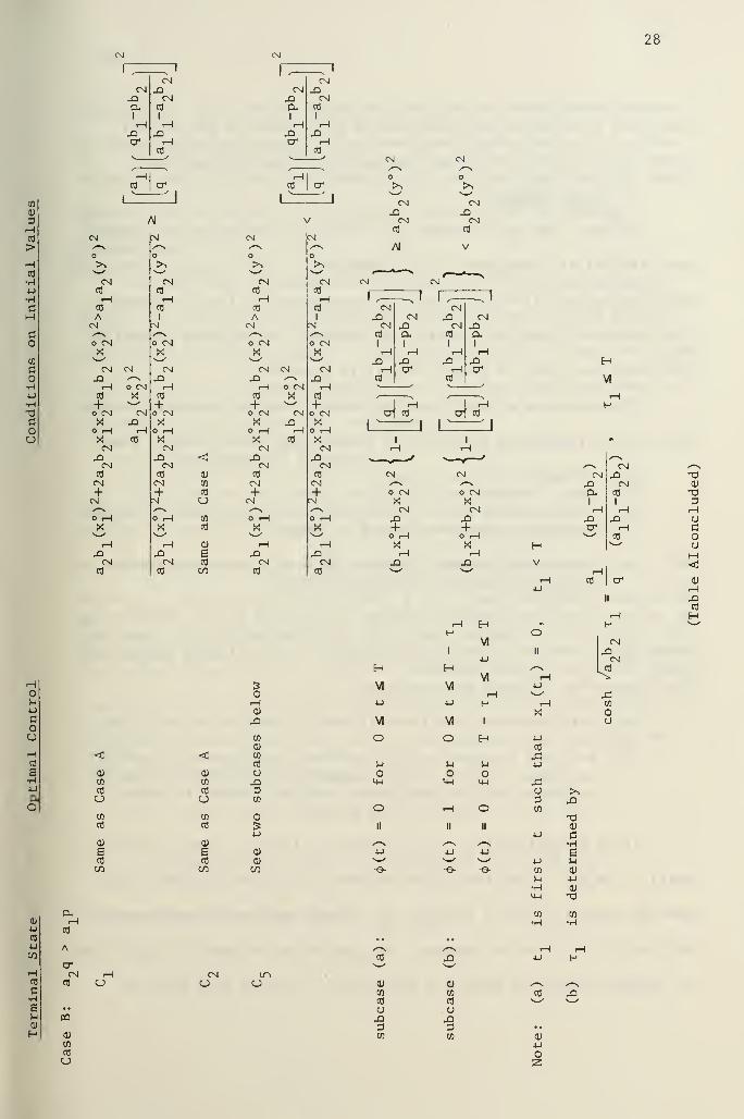
The complete solution to this problem is shown in Table AI. Details

are presented below. A significant point to note is that the extremals

are unique (non-overlapping of domains of controllability) so that the

extremal control turns out to be the optimal control. This solution

procedure may be easily extended to terminal control differential games

(such as [82] in which the usual necessary conditions [12] were not

applied). We do this in Appendix B. However, in two-sided problems

this author has noted that domains of controllability may overlap and

CM

27

w•Ha•H

cu

4-1

o4-1

Xi

•H

3rHco

>

co

en

Co•H4J

•H

cou

cfl CM

rH /—Vcd

r^A **—

'

HCM cO

/^*S

o CN VIXv^ o CNCN XX O rHH XIT) CN

XI+

CNo CNX +

o ,HX CMCN '—

\

r<a O rHCN X

CO

r̂HCN rQ

+CM

>>^-'

CNCO

rHCO

V

CM

CNX

CNXrH

CO

+o CNXo ^XCNXCN

crj

CN

+CM

CO CMrH ^~.

CO o>>

A \srH

CM CO

s~\o CN AX^~

'

o CNCN XX r-i

rH XCO CN

X+

CNo CNX +rHX CM

cO

CN

+CM

e

rHXoUP-,

o•H4->

OCD

rH0)

en

4-J

<u

uCO

H

CO•H4J

3rHoCO

X x

CN

cd

A

OU•u

coo

CO

e•H4J

D-O

4-t

VI

•u

VI

o

uoM-l

HVI

4-1

VI

rH HJ

VIVI

4-)

VI

o

r4

O<4H

VI

uoMH

OII

HVI

4-1

VI

o

4-J

-e-

<

rH

H

r-

cd

Co•H4-1

CX

IwwCO

cO

a)4-1

cO

4-1

C/3

0)

H

CXrH

Cfl

VI

trCN

CO

WCO

O

OII

oA

U

OII

>^

U

o oo oA A

A II

/»"N •~s^~v H H /~\

H —

'

^—

'

Hn---/ rH CN ^^^">> X X >^

u

28

CM

CO

ACM

CMXrH

CO

+o CNXO rHXCNXCM

CO

CN+

CM

1

CMCN X

-Q CM(X CO

H rHX XIcr H

CO

rHCO cr

1"

1

o CM

CN

CO

+O CNX

CO CD

CM co

+ CO

N U4~\o rH en

X CO^—

'

H OJ

X eCM CO

CO CO

CM

CM

CMXai

HCT

CMCO

IHXH

cO

V

CM

CO cO

A 1

CM CM/"> s—\

o CM o CMX X

N-^ N '

CM CM CNXi /-> XH o CM rHcO X CO

+ v—

'

+o CM CM CMX X X

O rH rH O r-{

X CO XCM CNX XCM CM

CO CO

CM CM+ +

CM N

CM

cO

AJ

CMCO

V

CM

CM*"

X CNCM X

cfl a.

rH rHX XrH cr

CO

X CNCM X

CO arH rHX XrH cr

cfl

HV!

CTJ cfl cr) cfl

CM

o CNXCM

O rHX

CM

o CMXCMX+O rHX H

V

CM X T>X CM OJ

i

CO

1 3rH rH rHX X CJ

cr rH d>«'

cfl o>^s a

cr

cO

B•H4-1

OJ rHu COCO

•u Aon

cr<-t CMcd CO

C•H

E ..

u M<u

H OJ

Cfi

CO

U

CO

cfl

u

cfl

<u

Ecfl

an

O

sorHOJ

Xen

a)

< en

cfl

a) aen Xcfl 3u en

05 ocfl S

4J

OJ

E a)

cfl atco co

CJ a

II XCO

rH HrH H b H ^s

1

V!

4-1

oII

CMXCM

H HVI r-{

L«VI VI

rH4-1

X4J j-) H rH

Xen

OVI VI 1 o

o o H 4J

Cfl

XrJ u r4 4-)

O o OU-l IW 14-1 X

CJ

3 Xo rH O en

T3II II II

4-)

OJ

C•H

U 4-1 4-)

4-1

EV4

-e- -e- -o- en

r4

•HUH

en

•H

014-1

OJ"3

en

•H

cu a)

en en

cfl cO

a . CJ

X X3 3en en

o55

29

there may be multiple extremals from a given point in the initial

state space so that additional considerations must be employed.

c. Some Comments .

We note that the solution to a "fight to the finish" may depend

upon the initial strengths of the combatants. This should be contrasted

with the optimal allocation which is independent of force strength in

the prescribed duration battle. We contrast the solution properties

for these two cases in greater detail in Appendix C.

The examining of this solution process provides valuable insight

into the corresponding differential (supporting weapon system) game:

(a) devising solution process,

(b) understanding why no transition (switching) surface presentin original problem studied by Weiss,

(c) formulating a game which may possess a switching surface(optimal strategies change with time).

It is noted that the supporting weapon system game may be viewed as an

extension of this fire programming problem. The following aspects are

also noteworthy of these two problems:

(a) both represent simplest allocation problems of their type,

(b) both are terminal control problems (as opposed to tacticalwar games studied by RAND researchers: [14], [15], [34] it

is noted that the continuous version of these is Isaacs'

[50] "war of attrition and attack").

It is noteworthy that if the objective function were modified to

ry(T) - px (T) , then the entire solution to the new problem is the

same as shown for case A in Table AI , except that the optimal control

for entry to C is not unique. Any control which leads to this state

is optimal, since the payoff is always zero. Let us note that the

deletion of x from the objective function has caused nonuniqueness

in the solution and absence of a transition surface under any circum-

stances. We shall see that these observations are important for under-

standing the solution of the original version of Weiss' supporting

system game.

We note that the approach developed here for solving terminal

control attrition games is different than that used to solve pursuit

and evasion differential games. Some examples of the latter are worked

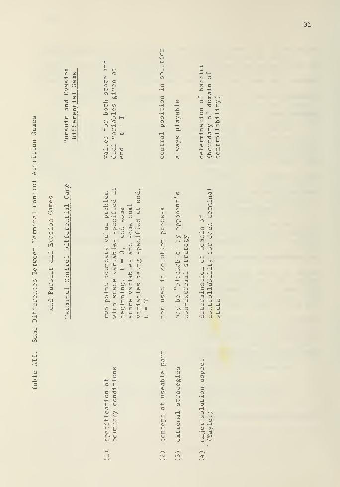
out in detail in a companion report [76]. In Table All we summarize

some major points of practical difference.

d. Development of Solution .

The solution is actually derived for a "reduced" game (that

portion of battle during which Y is faced with a choice problem).

We illustrate here for extremals to C. . It suffices to trace extremals

up to t when x (t1

) = 0, since <j>= from then until the end of

the game. The determination of the value, denoted by V(x ,x ,y) of

the reduced game, which is needed to determine the values of the adjoint

variables on the terminal surface, and part of the solution originally

obtained by Isbell and Marlow will not be repeated here although we

shall outline the general steps.

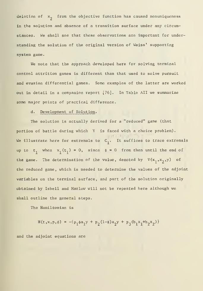
The Hamiltonian is

H(t,x,p,<}>) = -{p1

<})a

1y + p

2(l-4>)a

2y + p^b^+b^)

}

and the adjoint equations are

31

CO

QJ

6cfl

O3o•H4-1

•H)H

U4-1

<d

rHO>H

4-1

3 CO

O <uoi

1-1 aCO

c c•H o6 •HC CO

cu cfl

H >W

3CO XIQJ 3& cfl

4J

QJ 4-J

03 H3

w en

a) uo 33 Phoj

i-i X)CU s

14-1 cfl

M-l

•HQ0)

Boto

co 0)

H e03 CO

cfl o>W H

cO

X) •Hc 4-1

CO 3OJ

4-> H•H a)

3 4_|

(/I 14-1

u H3 aPm

X)cCD 4-J

CO

(U4J CCO 0J

4J >Cfl •H

60X4-1 en

o 0)

X HX H

n CO

o •H II

CH HCO 4-1

0] >OJ

3 HH CO x>CD 3 3> Xl <D

o•1-1

4-J

3rH

u

o •H 4-1

co S-i

S-J

o

C cO a•H X •H

CO

c M-l e —O QJ O O p^H rH XI 4-J

4-1 X c •H•H CO o M-l rHCO >, •H O -rH

O CO 4-J xta- rH cO >, cO

a. 3 U rHrn •H CO r-l

CO CO X) OJ-1 >^ r-l 3 U4-1 cO QJ 3 4J

3 3 4-1 o 3<u rH a) X Oo CO X) v~- O

4J #* rH6 co X) CO cd

aj 3 — 3rH XI a) 4-J •HXi QJ rH 3 EO -H cu CO 4-1 CO CD MVj iw e 3 crj CO 3 CD

a, -h o X) aj O UH 4J

CJ co X) o Cu oQJ QJ OJ OJ o cx X3 Cu XJ E •H u o 3 CJ

rH CO 3 o m a, •H CO

CO cO CO •H >^ >> CO OJ

> CO O 3 X 00 EQJ X) 0) o CD o H

>,rH •> 3 a •H E 4-1 X) or-l X o cO CO •U OJ CO M-l

CO cO 3 rH u M-l

XI -H II CO ao rH X 4-1 o J>!

3 M CD 3 O CO CO 4-1

3 cO 4-1 rH •H CO M 3 •HO > X cu a rH o rHX cO x> 3 o CO •H •H

CU > •H •H rH £ 4-1 X4-1 4-1 00 M to X aj cO cfl

3 cO 3 CO a) XI u 3 rH•H 4-J •H > rH 0) 4J •H rHO CO 3 XI CO CD X 6 oa* 3 OJ CO H 3 X OJ M J-l <U

x •H 4-J •H 1 aj 4-1 4-1

O 4-1 M CO t-i II 4-1 >> 3 4J 3 cO

3 -H cu 4J cO o Cfl O aj O 4J4-. rs x CO > 4-J 3 £ 3 XI CJ CO

<OJ

rHXCO

H

CO

3O

CM •HO 4-1

•H3 X)O 3•H O4-1 CJ

CO

CJ >^•H (H

M-l CO

•H X)a 3CD 3a OCO X

r-l

cO

PnCO

QJ QJ

rH •HX 00CO QJ

OJ 4-1

CO Cfl

3 S-i

4-J

M-l CO

orH

4J CO

a. 6QJ cuCJ u3 4-1

o XCJ QJ

CJ

QJ

CuCO

cfl

3O•H4-1

3rHO /-"N

CO S-i

oJ-l rHo >.•r-l cO

cfl HS ^

32

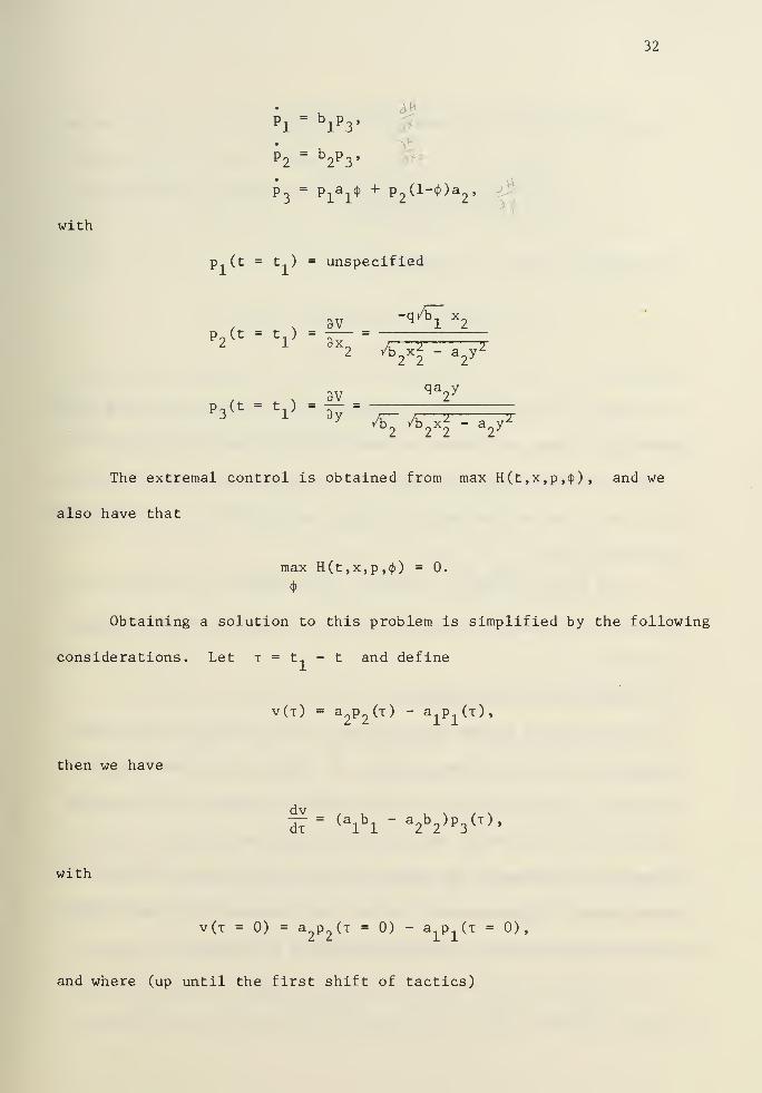
with

Pl

= blP 3'

P2

= b2p3

,

P3

- P^ +p2(l-*)a2>

p.. (t = t.. ) = unspecified

Po(t - t.) =2 * 8X

2 /b^ - a2y^

p Q (t = t,) =3 1 3y r— rr 7 7"

/t>2

/t>

2xj - a

2yz

The extremal control is obtained from max H(t,x,p,4>), and we

also have that

max H(t,x,p,<J)) = 0.

Obtaining a solution to this problem is simplified by the following

considerations. Let t = t. - t and define

v(t) = a2p2(i) - a p (t),

then we have

o7= (a

lbl

" a2b2)p

3(T) '

with

v(x = 0) = a2p2(x = 0) - alPl (x = 0)

and where (up until the first shift of tactics)

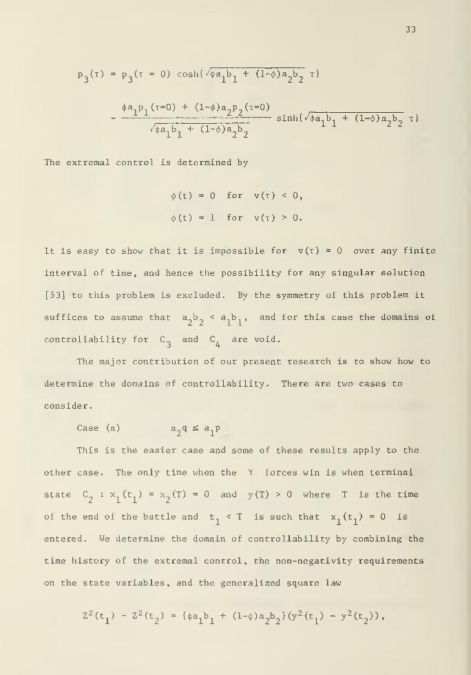
33

p (t) = p3(t = 0) cosh{/(|)a

1b1+ (H)a b t}

<|)a

1p1(T=0) + (l-<|>)a

2P2(T=0)

sinh{/(f)a b + (H)a b„ t}

The extremal control is determined by

4)(t) - for v(t) < 0,

c))(t) = 1 for v(t) > 0.

It is easy to show that it is impossible for v(t) = over any finite

interval of time, and hence the possibility for any singular solution

[53] to this problem is excluded. By the symmetry of this problem it

suffices to assume that a9D9

K aiD

i > an<^ f° r this case the domains of

controllability for C~ and C. are void.3 4

The major contribution of our present research is to show how to

determine the domains of controllability. There are two cases to

consider.

Case (a) a q £ a p

This is the easier case and some of these results apply to the

other case. The only time when the Y forces win is when terminal

state C : x (t ) = x (T) = and y(T) > where T is the time

of the end of the battle and t.. < T is such that x1(t

1) =0 is

entered. We determine the domain of controllability by combining the

time history of the extremal control, the non-negativity requirements

on the state variables, and the generalized square law

Z 2 (t1

) - Z 2 (t2

) = Ua^ + (l-^)a2b2}(y 2 (t

1) - y

2 (t2)),

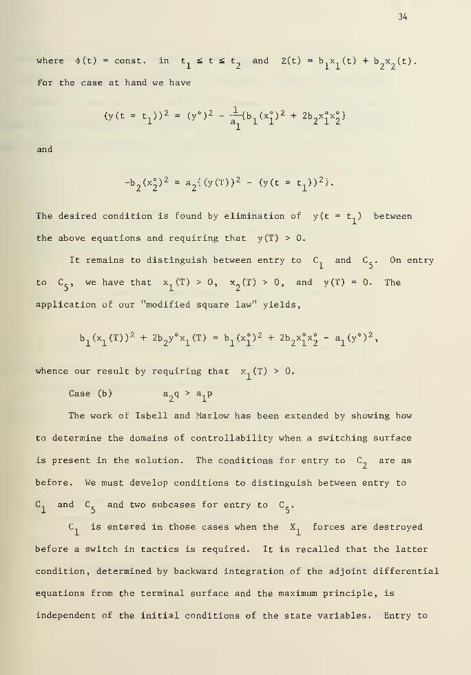
34

where <j»(t) = const. in t £ t £ t and Z(t) = b x (t) + b x (t)

For the case at hand we have

(y(t =tl ))

2 = (y°) 2 - J41,(X£)2 + 2b

2x°x°}

and

-b2(x°) 2 = a

2{(y(T)) 2 - (y(t = t^) 2

}.

The desired condition is found by elimination of y(t = t1

) between

the above equations and requiring that y(T) > 0.

It remains to distinguish between entry to C and C . On entry

to C , we have that x (T) > 0, x (T) > 0, and y(T) = 0. The

application of our "modified square law" yields,

b1(x

1(T)) 2 + 2b

2y°x

1(T) = b

1(x°) 2 + 2b

2x°x° - a^y )

2,

whence our result by requiring that x.. (T) > 0.

Case (b) a q > a p

The work of Isbell and Marlow has been extended by showing how

to determine the domains of controllability when a switching surface

is present in the solution. The conditions for entry to C„ are as

before. We must develop conditions to distinguish between entry to

C and C and two subcases for entry to C .

C. is entered in those cases when the X1

forces are destroyed

before a switch in tactics is required. It is recalled that the latter

condition, determined by backward integration of the adjoint differential

equations from the terminal surface and the maximum principle, is

independent of the initial conditions of the state variables. Entry to

35

C. is determined by the relationship between the proportion of total

battle time (forward) to destroy X.. and the time (backward) of the

potential switch. The figure below shows the relationship between

these times, where t = T - t, T- is the time (backward) of the switch,

t = t1

is such that X (t ) = 0, and T is the time (forward) of the

end of the battle. As shown C would be entered.

(T-t1

) >

t=0 t=t. t=T

The condition for entry to C. is that t > t1

where T = t + t ,

i.e. , the optimum length of x-time for engaging X_ is less than the

remaining time for X?

to destroy Y after Y has annihilated X..

(battle starts with engagement of X ). From the "modified square law,"

y( t = t±

) = /(y°) 2 - (x°) 2 - 2o o

xiV

After annihilation of X.. , there is another battle of length t„

remaining. Hence, for this portion where t.. £ t £ T,

(t) = y(t = t1)cosh/a

2b2(t - t

±) - - sinh/a b (t - t

n ).2 a 2 2 1

Since y(t = T) = 0, we have (using that T - t. = t )

36

y(t=t1

) fT

From integration of the adjoint equations and the maximum principle,

the x-time of the switch is given by,

\ (qb1~pb

2)

cosh/a_b t 1= — , , r~r •

2 2 1 q (a1b1~a

2b2

)

The desired condition is determined by requiring that t„ > x (as

defined above) , use of the identities

cosh *x = lnfx + /x 2 - l]

tanh

and considerable algebraic manipulation.

It finally remains to distinguish between the two cases of entry

to C . If \\>{t) = for <; t <; T, then

(bX + b?x°)

^7

1 1 9 9

'

y(t) = y° cosh/aTbT t - sinh/a„b„ t.I z j

—-

—

z 2

The boundary between the two cases is when y(T) = for T = x and

hence,

(b x° + b9x°)2

(y°) 2 [cosh/aTbT t.] 2 =K {[cosh^^T xj 2 - 1}11 1 a_ d 11 1

37

where cosh/a b t is given as above. Noting that <j)= for the

entire battle when T < x1

and re-arranging, we obtain the result

shown in Table AI.

e. Structure of Optimal Allocation Policies .

For square law attrition it may be shown that the allocation of

fraction of fire is always or 1 (see previous section for remark)

,

and fire is concentrated on one target type. This is not surprising,

since our model assumes complete and instantaneous information [13] and

that fire may be immediately shifted to a new target once the old one

has been destroyed [22], [81].

With reference to Table AI , the condition that a,b > a b„ may

be interpreted to mean that there is more long range return for Y to

engage X , i.e., more Y's will survive if this is done. Hence,

when Y wins, he always engages X ' s while they are available. The

condition a..p < a q means that at the end of battle there is greater

payoff per unit time per Y soldier to engage X not considering X1

'

s

greater attrition effect against Y (short term gain at end of battle)

.

By the maximum principle and the well-known interpretation of the

dual variables [12], Y always allocates his fire entirely to the

target type yielding the greatest marginal return. However, marginal

return evolves differently in winning or losing causes. When Y loses,

he may switch from firing at X.. entirely to firing at X entirely

before the X force has been annihilated. This happens when Y assigns

utility to survivors of force type X?

in excess of their kill rate

against Y as compared to force type X , and X is abundant enough

not to be destroyed before the battle ends.

38

In this way, we see that tactics may depend on force levels. We

also see that Y's target priorities only switch with time in a losing

case. This has occurred since a boundary condition at t = T on one

of the dual variables is dependent upon values of the state variables

by a transversality condition. It may be shown that the structure of

optimal allocation policies is different for the prescribed duration

battle.

In Appendix F we show how such considerations as those discussed

above may be developed into the concept of a dynamic kill potential.

However, we do so from the standpoint of the adjoint system for a system

of differential equations. (This approach may be used as an alternative

to that of Pontryagin for the development of his maximum principle.)

39

APPENDIX B. H. K. Weiss' Supporting Weapon System Game

In this appendix we develop the solution to the supporting weapon

system game of H. K. Weiss [82] by applying the theory of differential

games. Previously, this problem had been solved under restrictive assump-

tions by heuristic means. The solution procedure developed here is general

and applies to any terminal control attrition game. A new solution concept

is motivated by this development, and solution behavior not previously noted

for differential games is encountered.

Our researches on this and similar dynamic tactical allocation problems

indicate that there are several significant differences in theory and re-

sults between attrition and pursuit-evasion differential games. We have

briefly considered such differences in Appendix A. However, much excellent

research has been done on generalized control theory applicable to pursuit

and evasion problems, and we envision the application of such results to

tactical allocation problems as being fruitful future research. For example,

the concepts of stochastic control could be applied to a situation in which

combatants select targets without knowing precisely what the results of

firings will be.

The model considered here is an idealization of a real combat situation.

Its value lies in the insight it provides into the relations between system

parameters. It should not be expected to produce a numerical answer to a

specific problem but rather to indicate general principles to serve as hy-

potheses for subsequent computer simulation studies or field experimentation.

In this manner, the model considered here may be used to study the following

40

facets of supporting weapon systems: performance characteristics, alloca-

tion rules, impact of intelligence and command and control factors on the

preceding.

There are two types of scenarios in which we may study idealizations

of tactical allocation problems: (1) the prescribed duration battle and

(2) the terminal control battle, i.e., the game only ends when the course

of battle has been steered to a prescribed state. All the attrition prob-

lems studied by Isaacs [50] are of the first type. It is noted that his

War of Attrition and Attack is the continuous version of other such studies

[14], [15], [34]. Only Isbell and Marlow [52] and Weiss have studied the

terminal control problem. The former did not obtain a complete solution

to their problem but we have in Appendix A and were motivated to the

present development. Only by studying several types of models can we begin

to understand the dependence of allocation rules on model form.

In this appendix we consider what forms of such dynamic models are

available before we review Weiss' problem formulation. We then critique

his previous approach before outlining our new solution procedure and pre-

sentingdetails of solution development. We then discuss the structure of

optimal allocation policies. We also discuss extensions of the model and

a pitfall of model formulation before we contrast some facets of prescribed

duration battles to fights to the finish. We finally mention a few implica-

tions of the models we have considered. In view of the intimate relation-

ship [12] , [41] between optimal control theory and differential games

(Isaacs), we use their terminology somewhat interchangeably.

41

a. Forms of Model Available .

It seems appropriate to discuss the factors affecting the optimal

allocation policies. Different assumptions regarding these factors lead

to models with different optimal allocation policies. The model for a

tactical allocation problem involves three factors:

(1) the payoff,

(2) the description of combat,

(3) the planning horizon.

We will consider a terminal payoff with a linear objective function.

The tactical allocation problems studies at RAND [14], [15], [34], [50]

all involved an integral payoff. Further comment on the effect of inclu-

sion of only one of the two force types in the payoff by Weiss [82] seems

appropriate. What effect does this have on the optimal allocation? From

the present work, it seems reasonable to conjecture that for two-on-two

combat the optimal strategies for a side will be constant over time (except

for the obvious change when a force under attack becomes exhausted) if the

payoff only includes one force type. It is further conjectured that this

is the reason (only the "men" of each side appearing in the payoff) that

the optimal strategies in the reduced supporting weapon system game of

H. K. Weiss are constant over time and that optimal strategies may vary

over time when all force types are included in the payoff function. It

will be seen that optimal strategies only change over time for the loser

who engages the force type that does him the most damage in the early

stages of the battle and the force included in the payoff on which he has

the most effect in the latter stages. We conjecture that the winner's

optimal strategy is always constant over time for "fights to the finish."

42

For our description of the combat attrition process we may consider

a generalized Lanchester linear law or a square law (although other mathe-

matical descriptions have been noted as applicable to specific situations).

For a square law attrition process the attrition rate is proportional to

enemy strength, while for a linear law it is proportional to the product

of both enemy and friendly force strengths. With rare exception ([75] or

Isaacs' "war of attrition and attack: second version" [50]), previously

published work has considered only the square law model. In Appendix C

we show that a square-law attrition process leads to a "bang-bang" optimal

control while the linear law leads to a singular solution (see p. 481 of

[6]). The mathematical development is much more complex in the second

case, but we have studied singular problems on numerous occasions (pursuit

and evasion [76], inventory theory, the continuous version of Bellman's

stochastic gold-mining problem)

.

It seems appropriate to briefly discuss the physical assumptions which

underlie these idealizations of combat attrition. The square law arises

under conditions which include that "each unit is informed about the loca-

tion of the remaining opposing units so that when a target is destroyed,

fire may be immediately shifted to a new target" as noted by Weiss [81]

.

It is noted that differential game theory itself assumes complete informa-

tion (except that a player does not know the instantaneous strategy of the

opposing player) . The linear law arises when either target acquisition is

subject to diminishing returns [22] or fire is not redirected towards sur-

viving targets after attrition occurs [39], [70], [81].

In the present work a model is formulated for the simplest case of

partial information : "area fire" is delivered by the supporting weapon

system against the ground troops who use a constant area defense while the

43

perfect information assumption is retained on the state of the supporting

weapon system. Again quoting Weiss [81] , we assume that the supporting

weapon system units are informed about the general areas in which the

opposing infantry units are located but are not informed about the conse-

quences of their own fire. Thus, we see that we may account for some

changes in the information set by modifying the description of combat. Un-

fortunately, the mathematics of the resulting problem is much more complex

than previously encountered, and a complete solution has not yet been ob-

tained for this case. For this model of incomplete information, one in-

troduces the concept of inferred information (players know more than they

can observe directly) based on each player's knowledge of the time history

of his control variables and considers the resulting equations in this

light.

Another factor having a bearing on the optimal allocation policies

is the length of the planning horizon (length of the battle) . The follow-

ing three alternative models are available:

(1) battle of prescribed time duration,

(2) battle of unspecified time duration,

(3) battle until the extermination of one side.

Our researches have subsequently yielded that case (2) is not a properly

posed problem in the classical sense [27]. Models applying to the first

instance have been extensively studied by RAND researchers [14] , [15]

,

[34], [50]. The present work (as an extension of the work of Isbell and

Marlow and Weiss) will address the third case, "fights to the finish."

The mathematical details of solution and the structure of optimal policies

are significantly different for these two cases. Games of

44

prescribed duration are mathematically simpler than "fights to the finish,"

since the terminal surface consists of one "piece" and many different

portions do not have to be considered. Once the adjoint equations have

been integrated backward from the terminal surface, the history of the

extremal strategies (and hence optimal strategies) becomes uniquely deter-

mined unless a state variable goes to zero and a subgame is entered. On

the other hand for a terminal control game, extremals to all the distrinct

portions of the terminal surface must be considered. Entry to a portion

of the terminal surface must be verified by both considerations "in the

large" and forward integration of the state equations (after determination

of extremal strategies) . Many times the potential existence of a transi-

tion (switching) surface turns out to be illusory, and the complete solu-

tion may turn out to be radically different than was initially anticipated.

b. Problem as Formulated by Weiss

The problem studied by Weiss [82] may be stated as how should the

fire support systems of two heterogeneous forces (each consisting of

ground forces and its fire support system) optimally engage the opposing

combatant. The objective is for each side to minimize its losses in a

conflict which terminates when the opposing side is annihilated. The

ground forces (infantry) are assumed to have a negligible effect in pro-

ducing casualties on each other.

Using Weiss' original notation the problem was finally reduced to

the payoff:

max min [y (T) - y 9(T)]

,(Bl)

45

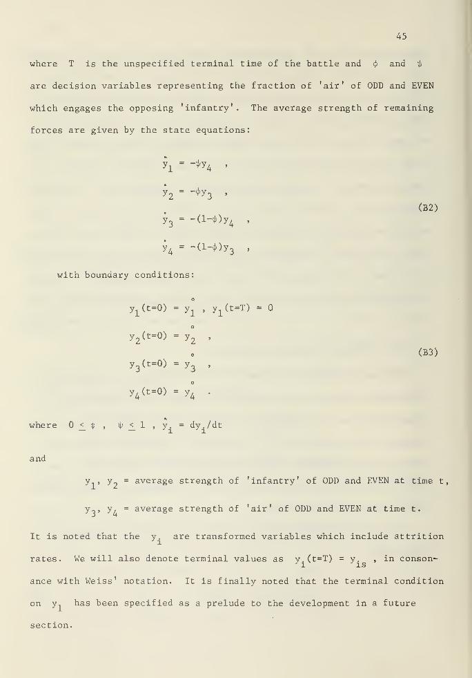
where T is the unspecified terminal time of the battle and <j> and ty

are decision variables representing the fraction of 'air' of ODD and EVEN

which engages the opposing 'infantry'. The average strength of remaining

forces are given by the state equations:

yx

= -^4 »

y2= -*y

3,

y3

= -(l-^)y4

,

y4= -(1-4) )y

3,

with boundary conditions:

(B2)

yiCt=0) = y

±,

y;L(t=T) =

(B3)

y2(t=o) = y

2,

o

y3(t=0) = y

3,

y4(t=0) = y°

.

where <_<J>

, ip <_ 1 , y . = dy./dt

and

y1

, y 9= average strength of 'infantry' of ODD and EVEN at time t,

y„, y, = average strength of 'air' of ODD and EVEN at time t.

It is noted that the y. are transformed variables which include attritioni

rates. We will also denote terminal values as y.(t=T) = y. , in conson-J1 is

ance with Weiss' notation. It is finally noted that the terminal condition

on y, has been specified as a prelude to the development in a future

section.

46

c. Critique of Previous Solution Procedure .

We should bear in mind that Weiss 's excellent paper [82] (it con-

tains much more than the mathematical solution of a differential game)

was written over ten years ago. Writing many years before results

were known beyond a small number of researchers, he did not employ the

usual (today's) necessary conditions [12]. The original solution

technique in this pioneering effort used unsupported assumptions which,

in general, are not true, although the correct answer was obtained to

the particular problem posed. Weiss assumed that optimal strategies

would be (a) either or 1 and (b) constant over time and then

determined the saddle point of the payoff function. It will be seen

that rather laborious computations are required to establish the solu-

tion form that Weiss assumed.

Weiss' s pioneering effort is especially remarkable when one con-

siders that Isaacs 's book [50] had not yet been written and only Isaacs 's

early RAND memos (see in particular [48], [49]) were available. Also,

Isbell and Marlow had failed to obtain a complete solution to a simpler

(one-sided) terminal control problem. We note that Weiss 's problem

(and also Isbell-Marlow fire programming problem) do not appear to be

known to the control theorists [5], [13], [24], [71].

Weiss 's paper also contains an extension of the attrition model

imbedded in an economic model of conflicting systems. It also contains

a penetrating analysis of weapon system performance characteristics

and concludes with a discussion of insight gained into the optimum

design of real world weapon systems.

47

d. Solution Procedure .

In this section we outline the solution procedure, introduce the

concept of the "reduced game," illustrate the determination of extremal

strategies, and discuss the concept of a "blockable" terminal state.

Outline of Solution Procedure

In a terminal control problem, we must determine the optimal strate-

gies for each player in terms of the initial conditions of combat (and

also possibly time). The solution procedure consists of two phases:

(a) determine all extremal strategies and (b) determine optimal strate-

gies from among the extremal strategies. By an extremal, we mean a path

on which the necessary conditions [12] for optimality are almost every-

where satisfied.

We must consider each terminal state separately. For each terminal

state, there will be one or more extremal paths leading to that state.

Extremal paths may be determined by routine application of the well-

known necessary conditions. For each extremal path to a terminal state

there is a domain of controllability, which we define to be that subset

of the initial state space from which a family of extremals leads to

the terminal state. The solution procedure may be summarized as:

(1) identify "attainable" terminal states,

(2) determine "domain of controllability" in initial conditionspace corresponding to each extremal leading to every"attainable" terminal state,

(3) partition the space of initial conditions into exhaustiveand mutually exclusive sets, each of which is covered by

the "domain(s) of controllability" of one, two, etc., of

the extremals to terminal states,

(4) the solution is uniquely determined at this point for regionscovered by part of only one domain of controllability,

48

(5) delete from further consideration those portions of thedomain of controllability of any terminal state which is

"blockable" from those initial points; again the solutionis uniquely determined (extremal is optimal) for thoseregions reverting to step (4)

,

(6) if there is still more than one extremal to a given terminalstate for a set of points in the initial condition space,compute the value of the game for each extremal; the finalsolution is determined by comparing these values.

The concept of a "blockable" terminal state is discussed below.

Concept of the "Reduced Game "

The battle is over when either y or y becomes zero. It is

convenient to introduce the concept of the "reduced game." Let us

henceforth refer to the original problem as the "realistic game." In

attrition games (especially "fights to the finish") the allocation

problem may disappear before the terminal surface is reached. Let us

refer to that part of the game for which the full allocation problem

exists as the "reduced game," and we now consider the terminal surface

of the reduced game. The value of the reduced game must be backcalculated

from the value of the realistic game. To illustrate, the terminal sur-

face for the above problem is defined by three terminal states: (a)

Yl (T) = 0, (b) y2(T) - 0, and (c) y^T) = and y

2(T) = 0. The

terminal surface of the reduced game is seen to consist of five portions

and these are shown in Table BI.

It will be seen that the extremal strategies to each of these

requires a different development. The payoff on C, is (-y (T)),

since ODD has lost all his infantry at the terminal surface of the

realistic game. It may be that a portion of the terminal surface is

not attainable from any point in the initial state space, and this is

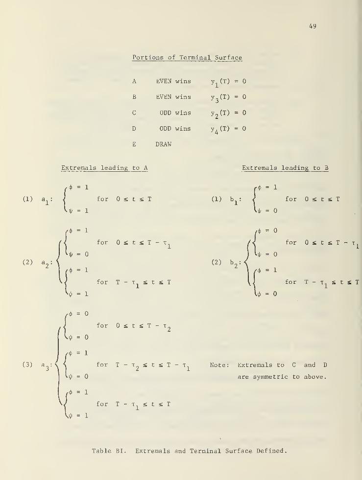
49

Portions of Terminal Surface

A EVEN wins yx(T) =

B EVEN wins y3(T) =

C ODD wins y2(T) =

D ODD wins y4(T) =

E DRAW

Extremals leading to A Extremals leading to B

(1) a1

: for £ t £ T

ip = 1

(1) b.

= 1

4 =

for £ t £ T

(2) a,

= 1

=

= 1

= 1

for <; t ss T - x.

for T - t £ t £ T

(2) b,

=

=

= 1

=

for £ t £. T - T.

for T - -t <. t £ T

.$ =

for £ t <; T - x

^ =

(3) a3 :{

^ =

V.

for T - x £ t £ T

for T - t £ t £ T

- t Note: Extremals to C and D

are symmetric to above.

4 = 1

Table BI. Extremals and Terminal Surface Defined,

50

what Isaacs refers to as the non-useable portion of the terminal surface

[50]. This concept is, however, not particularly useful in the solution

of an attrition game. The concept of the domain of controllability for

a terminal state is more useful.

Determination of Extremal Strategies

Table BI shows the five terminal states to the ("reduced") support-

ing weapon system game. Extremal paths are determined for a "reduced

game," which is that part of the game for which a full allocation

problem exists. For example, after y = 0, ODD uses<J>

= 1 until

EVEN's infantry is annihilated, and we only need consider up until that

time. Moreover, to determine boundary conditions on the dual variables

in the "reduced game," we must consider the payoff of the entire game.

We discuss this point further in the next section.

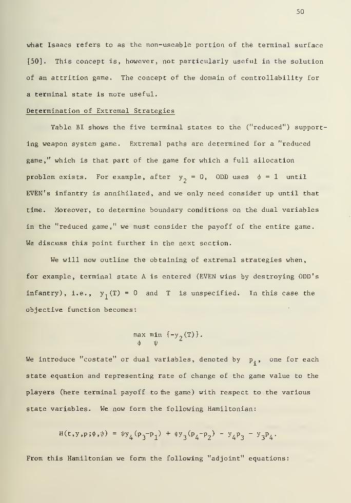
We will now outline the obtaining of extremal strategies when,

for example, terminal state A is entered (EVEN wins by destroying ODD's

infantry), i.e., y1(T) = and T is unspecified. In this case the

objective function becomes:

max min (-y 9

(T) }

.

«j> $

We introduce "costate" or dual variables, denoted by p., one for each

state equation and representing rate of change of the game value to the

players (here terminal payoff to the game) with respect to the various

state variables. We now form the following Hamiltonian:

H(t,y,p;<(>,(|j) = ij;y

4(p

3-p

1) + 4>y

3(p

4-p

2) - y^ - y^

.

From this Hamiltonian we form the following "adjoint" equations

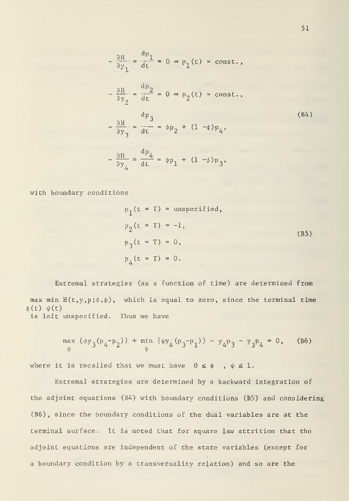
51

3Hdp

l__ = „ Pi(t) = const>)

_„_. o-p2(t) = const.,

dp3

(B4)

>Po + (1 -4>)P,,9y_ dt ^2 ^ T/ ^4

^77= JT = ^p i

+ (1 -^ )p3

:

4

with boundary conditions

(B5)

p.. (t = T) = unspecified,

p2(t = T) = -1,

p3(t = T) = 0,

p4(t = T) = 0.

Extremal strategies (as a function of time) are determined from

max min H(t ,y ,p ;<j> ,i|0 , which is equal to zero, since the terminal time

<Kt) MOis left unspecified. Thus we have

max Uy3(p

4-P

2)} + min {^(p^P-^l - Y

4P3

" Y3P4

= 0, (B6)

<j> i>

where it is recalled that we must have £ <|> , ty £ 1.

Extremal strategies are determined by a backward integration of

the adjoint equations (B4) with boundary conditions (B5) and considering

(B6) , since the boundary conditions of the dual variables are at the

terminal surface. It is noted that for square law attrition that the

adjoint equations are independent of the state variables (except for

a boundary condition by a transversality relation) and so are the

52

extremal strategies. The domain of controllability for an extremal so

determined is obtained by a forward integration of the state equations.

The non-negativity of the state variables plays a central role in these

determinations [74]. Details for the case at hand are presented in the

next section.

Concept of a "Blockable" Terminal State

It may be shown that for many regions of the initial state space

of this problem, there is more than one family of extremals leading to

terminal states. The reason for existence of multiple extremals is that

the min-max principle is merely necessary and of a local nature (see

Athens and Falb [6] for a discussion of the corresponding situation in

control theory). The attainable portions of the terminal surface are

not "close together" when multiple extremals are present.

A solution aspect unique to terminal control attrition games is

that in cases where there are extremals from the same initial point to

different terminal states corresponding to the same player both winning

and losing, entry to a terminal state may be "blocked" by the "losing"

player through use of an admissible strategy other than his extremal

strategy. In other words, there is a path determined by the necessary

conditions leading from each point in a region of the initial state

space to a terminal state, but the "losing" player may use a strategy

other than his extremal strategy to actually win. This behavior high-

lights the local ("in the small") nature of the necessary conditions

and the fact that the conditions are, indeed, necessary, i.e., assume

that the losing player cannot prevent the terminal state from being

reached.

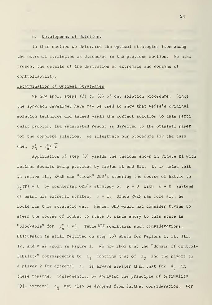
53

e. Development of Solution .

In this section we determine the optimal strategies from among

the extremal strategies as discussed in the previous section. We also

present the details of the derivation of extremals and domains of

controllability

.

Determination of Optimal Strategies

We now apply steps (3) to (6) of our solution procedure. Since

the approach developed here may be used to show that Weiss' s original

solution technique did indeed yield the correct solution to this parti-

cular problem, the interested reader is directed to the original paper

for the complete solution. We illustrate our procedure for the case

when y° = y°//2.

Application of step (3) yields the regions shown in Figure Bl with

further details being provided by Tables BI and BII. It is noted that

in region III, EVEN can "block" ODD's steering the course of battle to

y, (T) = by countering ODD's strategy of<f>

= with \p = instead

of using his extremal strategy i>= 1. Since EVEN has more air, he

would win this strategic war. Hence, ODD would not consider trying to

steer the course of combat to state D, since entry to this state is

"blockable" for y° > y°. Table BII summarizes such considerations.

Discussion is still required on step (6) above for Regions I, II, III,

IV, and V as shown in Figure 1. We now show that the "domain of control-

lability" corresponding to a contains that of a and the payoff to

a player 2 for extremal a is always greater than that for a in

these regions. Consequently, by applying the principle of optimality

[9], extremal a„ may also be dropped from further consideration. For

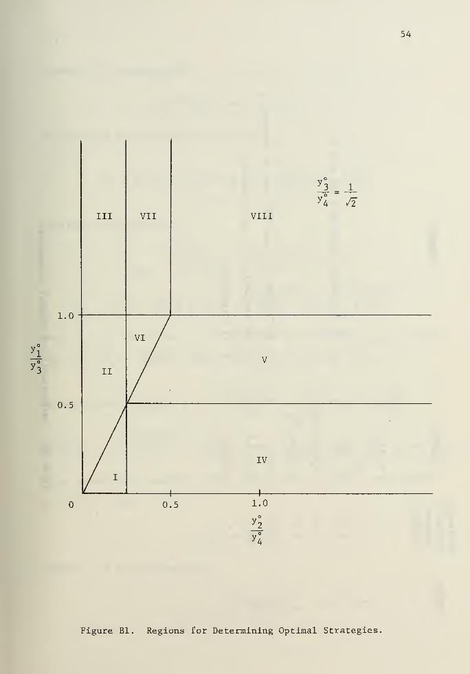
54

1.0 --

0.5

y 4

1_

/2

III VII VIII

VI /

V

II

/

IV

/ I

1 1 1

0.5 1.0

„o

Figure Bl. Regions for Determining Optimal Strategies.

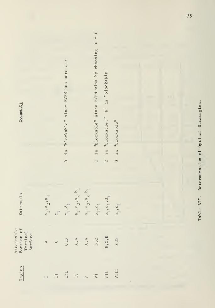
oII

55

c0)

ocj

u•Hco

CU

o6

0)

03

4=

W>w<u

oc•HCD

•s4*i

CJ

O

Q

ooG•H03

Oo

o

>>42

03

C•H

&

W>Wcu

acH03

42cO

4*i

CJ

o

CJ

X)CD

CJ

o

42cfl

ao

CJ)

42CO

ao

Q

03

OJ

•H00<u

cfl

u

c/3

CO

B•H4J

(XOM-l

O

ao•HJUCO

C•HE>-i

OJu0)

Q

CO

6cu

u•u

Xw

CO

CNl

coMMCQ

cu

i-rf

42CO

H

42CO

c•HCO

•U

HCO cu

a CJ

•H CO

e M-l

c Vj

0) 3H C/3

CJQCJ)

pq CQ CJ

CQ

QCJ

CQ

OCQ

CO•H00CU

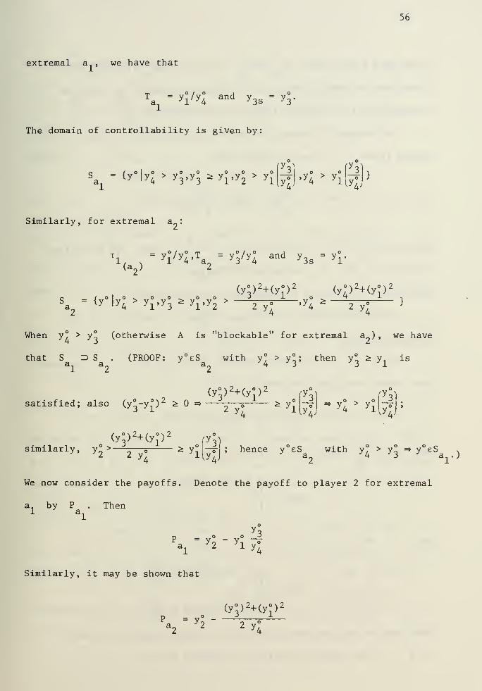
extremal a.. , we have that

Tai

=y«/y; and y 3s=

y ;.

The domain of controllability is given by:

56

sai

= fy%;>y"3,y;*y;,y°>y°

ry-

y 4<

o o' y

4> y

l y>

Similarly, for extremal a.

Tl,

," y

i/y

I-Ta, ' Jtf'4

and y 3s * "i-(a

2) 2

(yp2+<(y:)

2Cyl>

2+(y;>

2

s - {y |y4

> yr y3^ y

1,y

2> —y^ ,y

4*—^ }

2 44When y? > y° (otherwise A is "blockable" for extremal a ) , we have

that S 3 S . (PROOF: y°eS with y° > y°; then y° k y isa, a_ a_ 4 J j i

(y°) 2+(y°) 2

satisfied; also (y°-y°) 2 ^ =» —5 > y.iy/J

y4 " y

l uu

(yp2+(yp 2

similarly, y° > —-5 ^ y°* * y* x y/j

; hence y°eS with y° > y° =* y°eS ,

a_ 4 J a.. . ^

We now consider the payoffs. Denote the payoff to player 2 for extremal

an by P . Then1 a

l

\-y\-rx ^

Similarly, it may be shown that

(y°J2+(y;)

2

P = yl - % ol

a2

2 2 y4

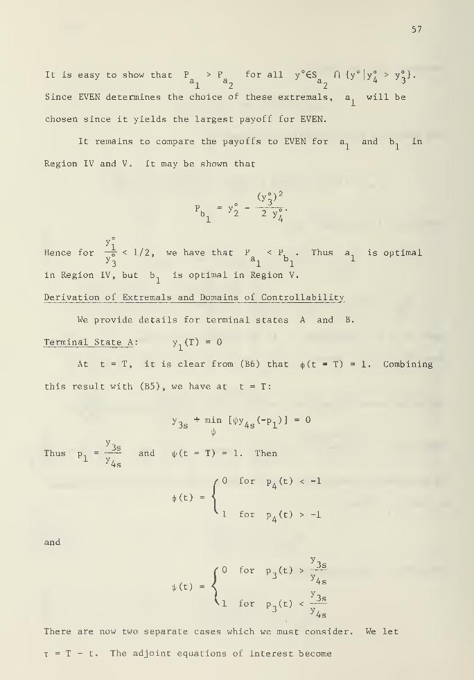
57

It is easy to show that P > P for all y°€S f] {y°|y? > y°}.a, a„ a_ 4 j

Since EVEN determines the choice of these extremals, a will be

chosen since it yields the largest payoff for EVEN.

It remains to compare the payoffs to EVEN for a1

and b1

in

Region IV and V. It may be shown that

(y°) 2

\ = y2

" "T^-

Hence for —5- < 1/2, we have that P < P, . Thus a. is optimaly3

ax

bx

1

in Region IV, but b1

is optimal in Region V.

Derivation of Extremals and Domains of Controllability

We provide details for terminal states A and B.

Terminal State A : y (T) =

At t = T, it is clear from (B6) that <()(t = T) = 1. Combining

this result with (B5), we have at t = T:

y 3s+ min ^y 4s (_P

l)] =

°

y 3sThus p = — and

ty(t = T) = 1. Then

Y4s

4>(t) =

for p (t) < -1

1 for p. (t) > -14

ana

y3s/0 for p

3(t) > -^

(« "\\1 for p (t) < -^

y 4s

There are now two separate cases which we must consider. We let

t = T - t. The adjoint equations of interest become

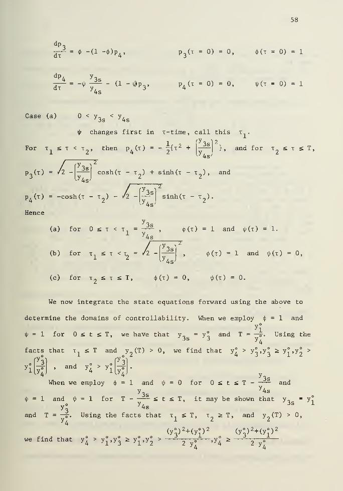
58

dp.

dx~-(1 -*)p

4, P

3(t = 0) = 0, 4)(t = 0) = 1

dp,

dx-*

r

4s(1 - 0P 3

, P4(t = 0) = 0, ^(t = 0) = 1

Case (a) < y < y.3s y 4s

ty changes first in x-time, call this x1

.

For x si x < T-, then p (x ) = - yH 2 +3s

^y4sJ} , and for x si x si T,

(x) = A -

x) = -cosh(x - x„) - /2 -P 4(T)

Hence

ly4s J

cosh(x - x ) + sinh(x - T-), and

3s

Ly4aJ

y3s

(a) for si x < x.. =,

y 4s

sinh(x - x2).

(b ) for x. si x < x_ = /2 -

T3s

4>(x) = 1 and 4>(t) = !•

, 4>(t) = 1 and iJj(x) = 0,

(c) for x2

si x si T,

y4s j

(x) = 0, iKt) - 0.

We now integrate the state equations forward using the above to

determine the domains of controllability. When we employ 4>= 1 and

i>= 1 for a: t S T, we have that y n = y° and T = —5-. Using the

3s y3 y,

4

facts that x <; T and y 2(T) > 0, we find that y° > y°,y° ;> y^.y? >

Ly.

ry-

, and y° > y°lyj

When we employ $ = 1 and ty= for si t si T -

"3s

isr

4s

and

3scf>

= 1 and ^ = 1 for T - si t si T, it may be shown that yy° y4s

and T = —5-. Using the facts that x si T, x £ T, and y„(T) > 0,y 4 1

(y°o)2+(y°) 2

(y°J2+(y°) 2

we find that y° > yj,y« > y°,y° >2 ^ ,y° *

2 /

— ,T

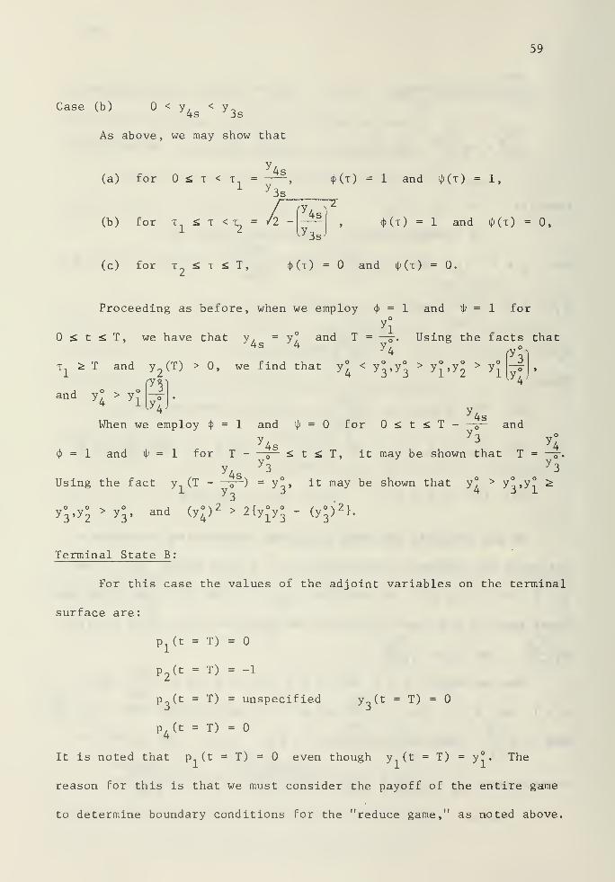
Case (b) < y. < y„

As above, we may show that

59

y 4s(a) for £ t < x =

y 3s

(b) for T, £ T < T„ = /2 -

(t) = 1 and iKt) = 1,

y 4s^

^y 3s^

<|>(t) = 1 and \\i(t) = 0,

(c) for t <. t <. T, 4>(t) = and i^ (t ) = 0,

Proceeding as before, when we employ cj) = 1 and<Jj

= 1 for

y-

£ t £ T, we have that y. = y° and T = —\

4s /4 y

Using the facts that

t1

^ T and y2(T) > 0, we find that y° < y°,y° > y°,y° > y°

ry«nand y° > y°

VI

ty/.

When we employ 4> = 1 and ip = for £ t ^ T - 4s

y.and

y4s

'3 y

4<|) = 1 and i>

= 1 for T - —5— £ t £ T, it may be shown that T = —

.

Us ^ ^Using the fact y (T - —3—) = y° , it may be shown that y° > yXfY^ ^

»\2y°3,y° > y°, and (y°)^ > 2{y°y° - (y°)^}.

Terminal State B :

For this case the values of the adjoint variables on the terminal

surface are:

p±(t = T) =

p2(t = T) == -1

p (t = T) = unspecified y (t = T) =

P4(t = T) =

It is noted that p (t = T) = even though y (t = T) = y° . The

reason for this is that we must consider the payoff of the entire game

to determine boundary conditions for the "reduce game," as noted above.

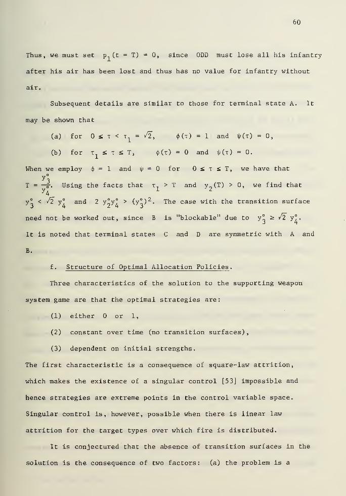
60

Thus, we must set p (t = T) = 0, since ODD must lose all his infantry

after his air has been lost and thus has no value for infantry without

air.

Subsequent details are similar to those for terminal state A. It

may be shown that

(a) for £ t < t = /2, <|>(t) = 1 and iJj(t) = 0,

(b) for t £ t £ T, <Kt) = and ip (t) - 0.

When we employ <j> = 1 and \p = for £ x £. T, we have that

y °3

T = —5-. Using the facts that xn

> T and y„(T) > 0, we find thaty4

12y° < Jl y° and 2 y°y° > (y°) 2

. The case with the transition surface3 4 24 3

need not be worked out, since B is "blockable" due to y° ^ vl y°.

It is noted that terminal states C and D are symmetric with A and

B.

f . Structure of Optimal Allocation Policies .

Three characteristics of the solution to the supporting weapon

system game are that the optimal strategies are:

(1) either or 1,

(2) constant over time (no transition surfaces),

(3) dependent on initial strengths.

The first characteristic is a consequence of square-law attrition,

which makes the existence of a singular control [53] impossible and

hence strategies are extreme points in the control variable space.

Singular control is, however, possible when there is linear law

attrition for the target types over which fire is distributed.

It is conjectured that the absence of transition surfaces in the

solution is the consequence of two factors: (a) the problem is a

61

terminal control one and (b) only one target type is in the payoff.

In a similar one-sided Problem [52], [74], such a switch in tactics

only occurs in a losing cause when both target types are weighted in a

terminal payoff. If we were to consider a prescribed duration battle,

then it may be shown that transition surfaces may occur for both sides

(compare with Isaacs' [50] War of Attrition and Attack). Inclusion of

only infantry in the payoff has the effect, in this case, of causing

air to always be direct at infantry during the last stages of battle.

It is conjectured that there can exist transition surfaces in the solu-

tion when all target types are weighted in the payoff. When this is

done, however, it may be shown that Weiss' s change of variables is

inappropriate (payoff must also be transformed) , and the original formu-

lation of the state equations with kill rate coefficients must be used.

Finally, it may also be shown that for the prescribed duration

battle target selection depends only on the attrition rates of the

various force types and relative weights assigned to surviving force

types. This should be contrasted with the terminal control case where,

as we have just seen, tactics depend on force levels. Thus, we see that

tactics depend on the circumstances under which the conflict ends, and

Weiss has written a fundamental paper [83] on this topic.

g. Extensions of Model .

It seems appropriate to discuss two extensions of Weiss' original

model: one extends the type of payoff and the other modifies the infor-

mation set available to the players. This second extension is believed

to be more descriptive of the deployment of a supporting weapon system

against ground forces. Complete solutions haven't yet been developed

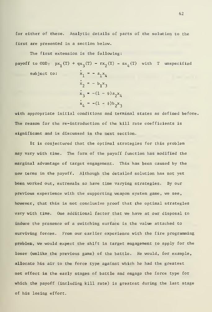
62

for either of these. Analytic details of parts of the solution to the

first are presented in a section below.

The first extension is the following:

payoff to ODD: px (T) + qx (T) - rx (T) - sx (T) with T unspecified

subject to: x = - a.x.J 114x2

= - blx 3

x3

- -(1 - \\))a2x^

x^ = -(1 - (f))b2x

with appropriate initial conditions and terminal states as defined before,

The reason for the re-introduction of the kill rate coefficients is

significant and is discussed in the next section.

It is conjectured that the optimal strategies for this problem

may vary with time. The form of the payoff function has modified the

marginal advantage of target engagement. This has been caused by the

new terms in the payoff. Although the detailed solution has not yet

been worked out, extremals so have time varying strategies. By our

previous experience with the supporting weapon system game, we see,

however, that this is not conclusive proof that the optimal strategies

vary with time. One additional factor that we have at our disposal to

induce the presence of a switching surface is the value attached to

surviving forces. From our earlier experience with the fire programming

problem, we would expect the shift in target engagement to apply for the

loser (unlike the previous game) of the battle. He would, for example,

allocate his air to the force type against which he had the greatest

net effect in the early stages of battle and engage the force type for

which the payoff (including kill rate) is greatest during the last stage

of his losing effort.

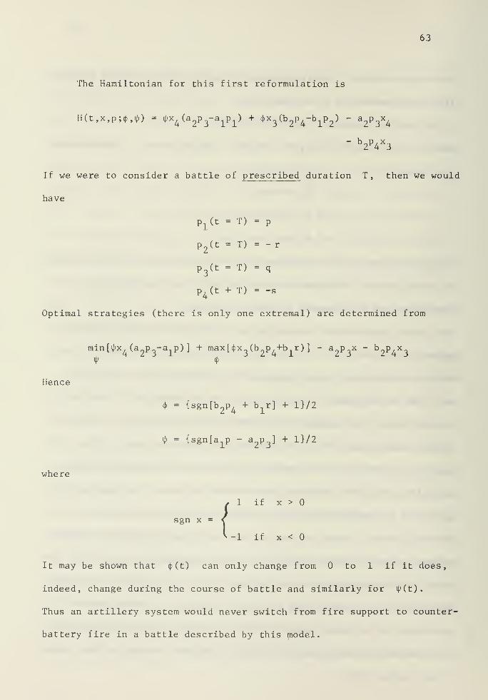
63

The Hamiltonian for this first reformulation is

H(t,x,p;<J>,ij>) = ^x4(a

2p3~a

1p1

) + <j>x

3(b

2p 4~b

lP 2^ ~ a

2P3X4

- b2P4x3

If we were to consider a battle of prescribed duration T, then we would

have

P-^t = T) = p

p2(t = T) = -

r

p3(t = T) = q

p4(t + T) = -s

Optimal strategies (there is only one extremal) are determined from

min[ipx4(a

2P3-a

;Lp)] + max^x^b^+b^) ]

- a^x - b^x*

Hence

= {sgn[b2P4+ b

]

_r] + l}/2

\p = {sgnj^p - a p ] + l}/2

where

, 1 if x >

sgn x = <

{ -1 if x <

It may be shown that <|)(t) can only change from to 1 if it does,

indeed, change during the course of battle and similarly for i> (t) .

Thus an artillery system would never switch from fire support to counter-

battery fire in a battle described by this model.

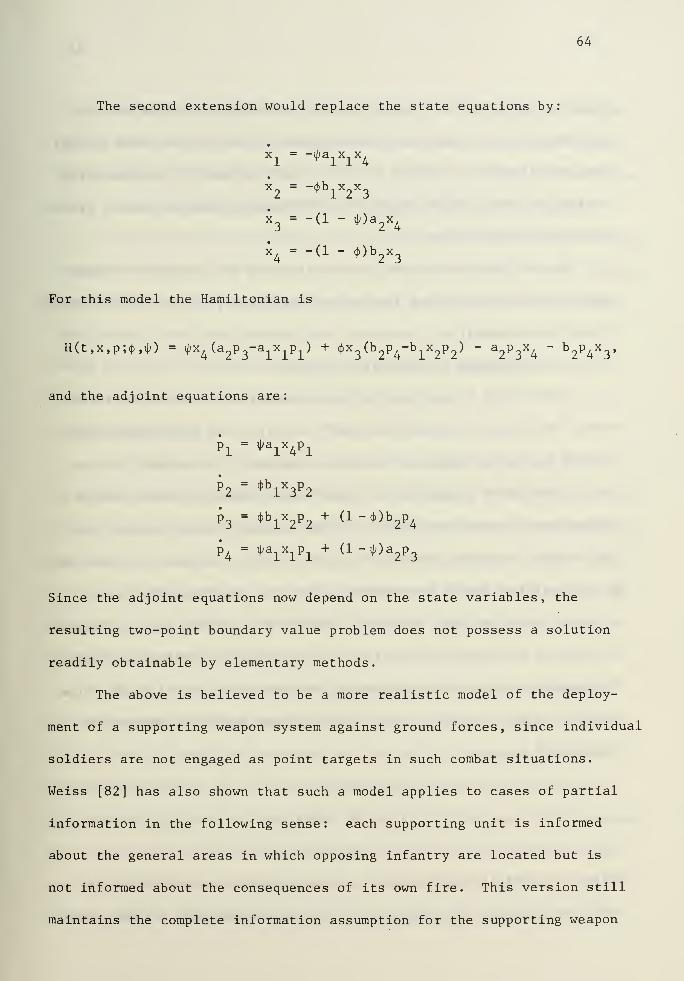
64

The second extension would replace the state equations by:

*1=

_,Jjalxlx4

X2

= -t))bix2x3

x3

= "(I ~ ,lJ ) a

2x4

x = -(1 - 4>)b>2x

For this model the Hamiltonian is

H(t,x,p;(J>,ip) = i|>x^(a p -a x^p ) + ^(b^-b^p^ - a2p3X4

" b2P4X3'

and the adjoint equations are:

Pi= ^a

ix4Pi

p2

- *b lX3P 2

P3

=*b

iX2P2+ (1 "* )b

2P4

P 4=

^alxipi+ (1 _l^ )a

2P3

Since the adjoint equations now depend on the state variables, the

resulting two-point boundary value problem does not possess a solution

readily obtainable by elementary methods.

The above is believed to be a more realistic model of the deploy-

ment of a supporting weapon system against ground forces, since individual

soldiers are not engaged as point targets in such combat situations.

Weiss [82] has also shown that such a model applies to cases of partial

information in the following sense: each supporting unit is informed

about the general areas in which opposing infantry are located but is

not informed about the consequences of its own fire. This version still

maintains the complete information assumption for the supporting weapon

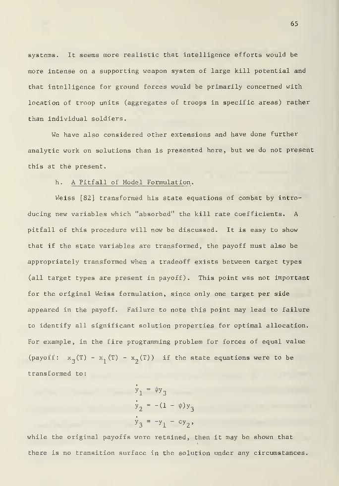
65

systems. It seems more realistic that intelligence efforts would be

more intense on a supporting weapon system of large kill potential and

that intelligence for ground forces would be primarily concerned with

location of troop units (aggregates of troops in specific areas) rather

than individual soldiers.

We have also considered other extensions and have done further

analytic work on solutions than is presented here, but we do not present

this at the present.

h. A Pitfall of Model Formulation .

Weiss [82] transformed his state equations of combat by intro-

ducing new variables which "absorbed" the kill rate coefficients. A

pitfall of this procedure will now be discussed. It is easy to show

that if the state variables are transformed, the payoff must also be

appropriately transformed when a tradeoff exists between target types

(all target types are present in payoff). This point was not important

for the original Weiss formulation, since only one target per side

appeared in the payoff. Failure to note this point may lead to failure

to identify all significant solution properties for optimal allocation.

For example, in the fire programming problem for forces of equal value

(payoff: x (T) - x (T) - x (T)) if the state equations were to be

transformed to:

h = *y3

y2

= -(1 - ^)y3

y3

--y-L

- cy2

,

while the original payoffs were retained, then it may be shown that

there is no transition surface in the solution under any circumstances.

66

It is conjectured that in the original version of the supporting weapon

system game this aspect of model formulation would have also prevented

the existence of time-varying optimal strategies under any circumstances.

i. Battles of Prescribed Duration and Fights to the Finish .

In this section we discuss some differences between the prescribed

duration battle and the terminal control battle (a special case of which

is the "fight to the finish"). We begin by contrasting various aspects

qualitatively and then present some solution details for one of the

model extensions mentioned earlier. We do so for both the prescribed

duration battle and the fight to the finish.

General Discussion

Of prime interest to the operations research worker who seeks

an understanding of complex phenomena, is the extent to which his choice

of model influences this perspective. We shall see that what determines

the end of a battle is very important to the combatants for their selec-

tion of optimal tactics. We shall contrast the battle for a prescribed

duration to the battle to a specified terminal state (in particular,

the "fight to the finish").

In all cases, target selection depends on the marginal return

for engagement. For the supporting weapon system game, marginal return

is the rate of change of the value of the game (in terms of forces

remaining) per unit of force allocated. It is measured by the product

of the rate of change of this value per unit of force type (dual variable)

and of the kill rate of this force type by the supporting weapon system.

Air or infantry is engaged depending on the difference of such quanti-

ties. Similar remarks apply to the fire programming problem. This

67

richness of interpretation of the dual variables is not present in the

analysis of multimove discrete games [14], [15], [34]. A very signifi-

cant point is that the type of model chosen (form of payoff function

and planning horizon) may lead to a different evolution of marginal

return. This is clear if one only considers the values of the dual

variables on the terminal surface. In the terminal control case, such

a value of one of the dual variables depends on initial strengths and

the history of the battle through the transversality condition

H(t = T,y,p ;<t>,40 = 0, whereas for the battle of prescribed duration

such values are independent of initial strengths.

In fights to the finish (extension one of section g) , a

commander must estimate the most vulnerable part of the enemy force

(both kill rate and force level) and then concentrate the entire fire

of the supporting weapon system on this. The winner continues with his

chosen strategy until the desired end is achieved. The loser may shift

fire to minimize his losses depending upon the weights he attaches to

remaining units of the winner's force types and his effectiveness

against each. For the battle of prescribed duration, on the other hand,

target selection is independent of initial strengths or tide of the

battle. If the battle lasts long enough, the optimal tactic may be to

shift fire regardless of whether one is winning or losing.

The fight to the finish is thus strongly dependent upon what are

the conditions under which a battle is ended, "the terminal states of

combat." It appears that there is more research to be done in this

important area, especially in view of the strong dependence of tactics

on it as pointed out in this paper. The excellent paper of Weiss' [83]

68

on Richardson's data should be noted. The current development may be

readily modified to termination at specified non-zero force levels.

There are no mathematical complications from this change.

Thus we conclude that a realistic model for optimal allocation

must also consider the conditions under which the battle terminates.

We could allow for replacements in such models. In such cases it might

be appropriate to consider total losses as defining an additional

terminal state. It may be necessary to consider different terminal

states for each combatant (not symmetric). For example, we could con-

struct a dynamic allocation model of guerrila warfare in which we might

consider the terminal state for the insurgents as reduction to a speci-

fied level (possibly zero) , while for the counter- insurgents (both sides

being allowed replacements) the end of the battle might be determined

by the length of the conflict (people get tired of war) and/or total

losses.

Of interest to the military tactician is whether target selection

rules evolve dynamically with the course of battle. Mathematically,

this may be stated as whether there is a transition surface in the solu-

tion. For the terminal control problems studied here, such a shift has

been conjectured to be present only in a losing cause. For battles of

fixed duration, the solution behavior is signigicantly different with

the possibility of transition surfaces being present for both sides.

Development of Solution to Prescribed Duration Battle

We consider the following problem (which has been formulated

from ODD's standpoint)

max min{px (T) + qx (T) - rx (T) - sx (T)} with T specified,

4 i>

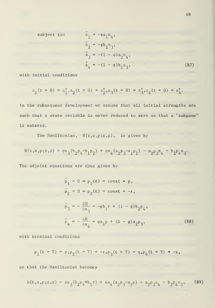
69

subject to: x = -^a..x, ,

X2

= _ct)bix3'

x„ = -(1 - i/i)a x,

x4

= -(1 - <j>)b2x3

, (B7)

with initial conditions

x±(t = 0) = x°,x

2(t = 0) = x°,x

3(t = 0) = x°,x

4(t = 0) = x°.

In the subsequent development we assume that all initial strengths are

such that a state variable is never reduced to zero so that a "subgame"

is entered.

The Hamiltonian, H(t ,x,p ;<{> ,ip) , is given by

H(t,x,p;cj>,40 = (f)x3(b

2P4-b

1p2

) + ijjx^ (a^-a.^) - a2p3X4 " b

2P4X3'

The adjoint equations are thus given by

p = => p1(t ) = const = p,

p = => p2(t) = const = -r,

h = - If:= -V + (1 " * )b2"V

h ' - If: - *v + (1 - *>w (B8)

4

with terminal conditions

px(t - T) - p,p

2(t = T) - -r,p

3(t = T) = q,p

4(t - T) = -s

,

so that the Hamiltonian becomes

H(t,x,p;<}>,ijj) = t{)x

3(b

2p4+b

1r) + ijix^a p -a p) - a

2p3x4 - b

2P4X3' ^ B9 ^

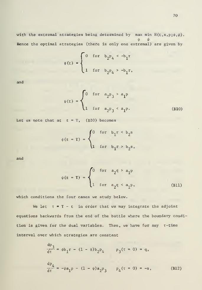
70

with the extremal strategies being determined by max min H(t ,x,p ;<|>,i|/)

.

Hence the optimal strategies (there is only one extremal) are given by

*(t) =

and

for b p, < -b,r

for b2P4

> -b][

r,

for a p > a p

*<t) =

1 for a2p3

< aLp. (BIO)

Let us note that at t = T, (BlO) becomes

(t = T) =

and

for b..r < b s

{1 for b..r > b s,

for a q > a..p

^(t = T)

1 for a2q < a p

,

(Bll)

which conditions the four cases we study below.

We let t = T - t in order that we may integrate the adjoint

equations backwards from the end of the battle where the boundary condi-

tion is given for the dual variables. Then, we have for any x-time

interval over which strategies are constant

dp3^~ = 4>b

1r - (1 - 4>)b

2P4

p3(x = 0) = q,

dp4

= -rpff_p - (1 - ^)a oP _ p. (x = 0) = -s, (B12)dT r~

L

r v ^ y/ "2 r3

vk

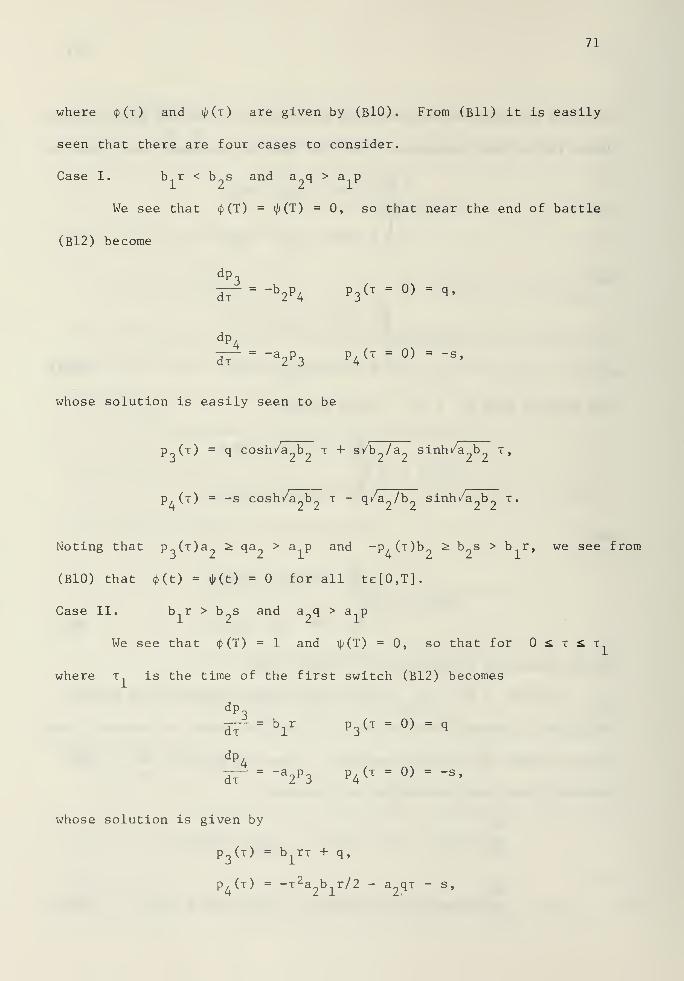
71

where<t> ("O and i^(t) are given by (BlO). From (Bll) it is easily

seen that there are four cases to consider.

Case I. b r < b s and a q > a p

We see that<J>(T) = \\) (T) = 0, so that near the end of battle

(Bl2) become

dp3

" -b oP/. Po( T 0) = q,dx "2 K4

r3

dp4

= -a P p, (x = 0) = -s,dx ~2^3 v

k

whose solution is easily seen to be

pJx) = q cosh /a b x + s/b /a sinh/a b x,

p, (x) = -s cosh/a b x - q/a /b_ sinh/a b x.

Noting that p (x)a„ ^ qa > a p and -p (x)b ^ b s > b r, we see from

(BlO) that <f>(t) = 4>(t) = for all te[0,T].

Case II. b r > b s and a q > a p

We see that <J>(T) = 1 and \p(T) = 0, so that for £ x £ x.

where x.. is the time of the first switch (B12) becomes

dp3

d7~= b2r p

3(x - 0) - q

dp4

Ir - -a2p3

p4(x = 0) = -s,

whose solution is given by

P3(t) = b

xrx + q,

P^(x) = -x 2a b r/2 - a2qx - s,

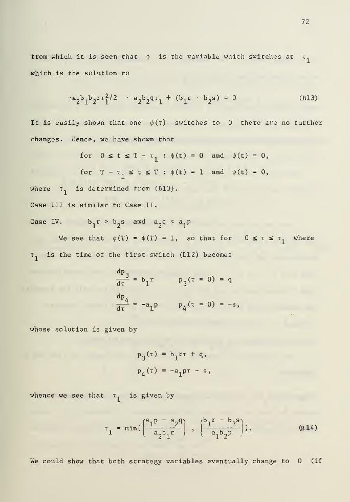
72

from which it is seen that<J>

is the variable which switches at T,

which is the solution to

-a b b2rx2/2 - a^qx + ( b

ir " b

2S ^

= ° (B13)

It is easily shown that one <K T ) switches to there are no further

changes. Hence, we have shown that

for £ t £ T - t : <f>(t) and \\)(t) = 0,

for T - x <; t £ T : <j>(t) = 1 and ip(t) = 0,

where x1

is determined from (B13)

.

Case III is similar to Case II.

Case IV. b..r > b s amd a q < a p

We see that <|>(T) = 4>(T) = 1, so that for £ i £ t where

T. is the time of the first switch (D12) becomes

dp.

dT

dT

bir

-alP

P3(t - 0) = q

p^d = 0) = -s,

whose solution is given by

P3(t) = b^^rx + q,

P4(x) = -a

1px - s,

whence we see that x.. is given by

T. = min{alP " a

2q

a2bir

bir " b

2S

{ aib 2p

(B14)

We could show that both strategy variables eventually change to (if

73

T is large enough). For example, if i> changes first at t , then

we may show that for t £ t £ t

P 4(t) = -a

2b1rt 2 /2 - a^x - s - (a p - a

2q)

2/ ^a^r) ,

so that p. (t) continues to decrease and $ may also change to 0.

In this example we have considered we would then have

for <; t £ T - x : <j>(t) = and ijj(t) = 0,

for I - t, i t i I - t. : <()(t) = 1 and iKt) - 0,

for T - t. i t < T : <Kt) = 1 and iji(t) - 1.

What we do want to point out from the above development is that

the optimum allocation of fire is independent of the force levels and

depends only on the attrition rates (and length of battle) . We also

note that if q = s = (only infantry weighted in the payoff) , then

Case IV above applies and the battle always terminates with the support-

ing weapon system fires concentrated on the ground forces possibly

preceded by a period of counterbattery fire.

Partial Development of Solution to Terminal Control Battle

We consider the following problem (again the payoff is from ODD's

standpoint)

max min{pxn(T) + qx„(T) - rx. (T) - sx. (T) } with T unspecified,

1 3 2 4

•

subiect to: x n= -ilia, x.,114

X2

= "*bix3'

x3

= -(1 - i|;)a2x^

x4

- -(1 - 4>)b2x3

,

74

with initial conditions

x±(t = 0) = x°,x

2(t = 0) = x°,x

3(t = 0)= x°,x

4(t = 0) = x°,

and terminal conditions similar to Weiss f

s original problem (see Figure

BI).

We will outline enough (hopefully) of the solution process to show

points of difference with the prescribed duration battle. Within the

framework of our solution procedure for terminal control attrition

games (see Section d above) , we have done only the first step (identify

terminal states and determine extremal paths).

As before, the Hamiltonian is given by

H(t,x,p;4>,iJ;) = <|>x (b^-b p )+ ^x 4 ^ a

2P 3~a

lPl^

" a2P3X4 " b

2P4X3'

(Bl5 ^

so that the adjoint equations are given by

p.. = - -— = =» p. (t) = const,1 3x 1

P2

= - 7j^~ = =» p (t) = const,

P3

= -|^= *b lP2 + (1 - «)b2p4

,

h = ~ f; *aipi+ (1 - ^ )a

2p 3- (B16)

4

From this point on the development is different for each terminal

state. We illustrate by considering the case when EVEN wins by destroy-

ing ODD's infantry, i.e., x (T) = 0. The boundary conditions at the

termination of the battle in this case are

75

p (t = T) = unspecified , x (t = T) = 0,

p2(t = T) = -r,

P3

( = T) = q,

p (t - T) - -s.

Extremal strategies are determined by max min H(t ,x,p ;<j> ,ij)) , which is

equivalent to

max{<() (b2P, + b r)}

,

and

min{iKa2p3

- a1P1)^ »

and, hence, extremal strategies are given by

*(t) =

and

<Kt) =

for b_p. < -b.r2 4 1

1 for b2P4

> -b1r,

for a2p3

> alPl (T)

1 for a2p3

< a p (T). (B17)

At t = T , we have

(t = T) =

and

*(t = T) =

for b r < b s

1 for b r > b s,

for a2q > a

;Lp1(T)

1 for a2q < a p (T)

,

(Bl8)

which gives us various cases to consider.

76

Since the termination time is unspecified, the following trans-

versality condition must be satisfied at the end of battle

H(t=T,x,p;4.,^) = 0. (B19)

We shall see that this condition has the effect of eliminating ii(t) =

as an optimal strategy for EVEN during the closing stages of battle.

We consider two cases of terminating conditions effecting EVEN's

strategy variable i\>.

Case A. a q > a p (T) implying 0(t = T) =

We show that this case is impossible and drop it from further

consideration. We have the following two cases to consider

(a) b1r < b s

By (B18), we have (j>(T) = so that (Bl5) and (B19) require that

-a qx + b sx = 0,2 4s 2 3s

where x. = x. (t = T) as used by Weiss. Since the above will, in

general, not be satisfied, this case is impossible.

(b) b r > b2s

By (B18) , we have <|>(T) 1 so that (B15) and (Bl9) require that

-a qx + bnrx = 0,

2 4s 1 3s

which likewise makes this case impossible.

Case B. a q < a p (T) implying \\i(t - T) - 1

Again, we have two subcases to consider

(a) b1r < b

2s

By (B18, we have (j> (T) = so that (B15) and (B19) require that

77

Pl (T) = (b2SX

3s)/(a

lx4s

) ' (B20)

so that Case B is given by

a_qx. < b_sx_ (B21)2 4s 2 3s

(b) bxr > b

2s

By (B18) , we have <|>(T) = 1 so that (B15) and (B19) require that

Pl (T) = (b1rx

3g)/(a

1x4s

), (B22)

so that Case B is given by

a2qx

4s< b

1rx

3s. (B23)

We will now investigate the above two subcases of Case B more

fully. Before we do this, let us rewrite the last two adjoint equations

(B16) in terms of the "backwards time" x = T - t

dp3^- = <(>b

1r - (1 - 4>)b

2P4

p3(t = 0) = q,

dp4-—- = -^a

lP;L(T)-(l - ^)a

2P3

p4(x = 0) = -s (B24)

As we have shown above, the terminal state x (T) = can only

be reached ween a q < a p (T) so that we have \\> (t = T) = 1. We

continue with the two subcases above.

(a) b nr < b_s and p n

(T) = (b o sx )/(a 1x. ) so that12 1 z is 1 4s

a qx < b sx2 4s 2 3s

By (Bl8) , we have <f>(T) = so that near the end of battle by

(B24) we have

d^ " "a lPl (T)

78

and P/( T )= _a

1P 1(T ) T - s < for all t.

Hence <£(t) - for £ t £ T. We may show that i(j(t) can switch to

at T.. , so we would have

for £ t <; T - x : <J>(t) = and ^(t) - 0,

for T - t as t <; T : <$>(t) = and \\>(t) = 1.

Determination of the domain of controllability is quite messy in this

case and we omit it at this time.

(b) b.r > b_s and p.. (T) = (b nrx_ )/(a,x. ) so that

1 2 1 1 js 1 4s

a qx. < b rx2 4s 1 3s

By (B18) , we have <t>(T) =1 so that near the end of battle we have

P^(t) = -a p (T)t - s

or

p. (t) = -b^x t/x. - s4 1 Js 4s

<(>(t) switches to at t given by

(bxr - b

2s)

T, =i*

blb2r

4s

x3s

and to summarize

for £ x < t : 4>(t) = 1

for t < t : <})(t) = 0.

Other details are similar to previous case.

j . Implications of Models .

It seems appropriate to discuss briefly the general implications

in the following areas:

79

(1) intelligence,

(2) command and control systems,

(3) human decision making.

Even though the present models assume complete and instantaneous

information, their solution does possess certain features capable of

being projected to cases where uncertainty is present. The selection

of tactics is seen to depend on a knowledge of the enemy's strength and

capabilities so that the appropriate target set may be chosen and optimal

strategies determined. Previous models [14], [15], [34] (battles of

prescribed duration) had not indicated such a conclusion but that tactics

depended only on enemy and friendly capabilities and length of combat,

not the initial force levels. For such models the estimate of the

combat length is critical, since if one were to extend this time, the

optimal strategies may have to be determined again from the beginning.

The shifting of tactics with time (instantaneously in the model)

indicates requirements for a responsive command structure. For the case

studied here, the loser of a battle may receive more benefits from a

command structure capable of implementing a change of tactics during

the confusion of combat.

Schreiber [70] has proposed "overkill" as a measure of "command

efficiency." His idea is to modify the description of combat to reflect

differences in command and control capabilities. One uses a linear law

(see Section g) when fire is not redirected from killed targets. How-

ever, we don't see the full implication of such diminishing returns in

combat here. In Appendix C we shall see that when there is a linear

law attrition process for the target types over which fire is distributed,

80

the nature of the allocation policy is fundamentally different.

These models may be interpreted to show the value of human judg-

ment in combat. They indicate, as does common sense and experience,

that in battle a commander must use his judgment to ascertain to what

end can the course of battle be steered so that he may devise his

strategy accordingly. The demonstrated sensitivity of these models to

many factors shows the importance of human assessment of a situation

and value attached to forces remaining after the battle at hand.

A further discussion is to be found in Appendix C.

81

APPENDIX C. Some One-Sided Dynamic Allocation Problems.

In this appendix we examine a sequence of problems to study the

dependence of optimal allocation policies on model form. The problems

are for combat over a period of time described by Lanchester-type

equations with a choice of tactics available to one side and subject

to change with time. We consider two types of choice problems: (1)

target-type selection and (2) firing rate.

In 1964 Dolansky [28] noted that the Lanchester theory of combat

was insufficiently developed in the area of target selection for combat

between heterogeneous forces (optimal control/differential games). This

remark was based on consideration of work by Weiss [82] and Isbell and

Marlow [52], both of which we have extended in previous appendices.

Since that time no further examples have been published in the litera-

ture except for the ones in Isaacs' book [50]. This previous work had

never systematically investigated the dependence of tactics on model

form.

With the first sequence of models our goal is to obtain insight

into optimal target selection rules in real combat by gaining a more

thorough understanding of some simple models and the solution character-

istics of such models. To understand the operations of a complex

system, many times the researcher examines a sequence of models of

greater and greater complexity to try to see if he can discern a "law

of nature." In the first two models we shall see how the objectives

of the combatants and the termination conditions of the conflict

influence target selection through the evolution of marginal return.

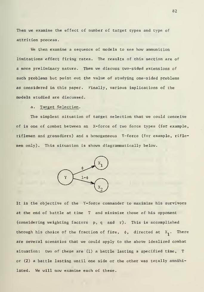
82

Then we examine the effect of number of target types and type of

attrition process.

We then examine a sequence of models to see how ammunition

limitations effect firing rates. The results of this section are of

a more preliminary nature. Then we discuss two-sided extensions of

such problems but point out the value of studying one-sided problems

as considered in this paper. Finally, various implications of the

models studied are discussed.

a. Target Selection .

The simplest situation of target selection that we could conceive

of is one of combat between an X-force of two force types (for example,

riflemen and grenadiers) and a homogeneous Y- force (for example, rifle-

men only). This situation is shown diagrammatically below.

It is the objective of the Y-force commander to maximize his survivors

at the end of battle at time T and minimize those of his opponent

(considering weighting factors p, q and r) . This is accomplished

through his choice of the fraction of fire, <j> , directed at X1

. There

are several scenarios that we could apply to the above idealized combat

situation: two of these are (1) a battle lasting a specified time, T

or (2) a battle lasting until one side or the other was totally annihi-

lated. We will now examine each of these.

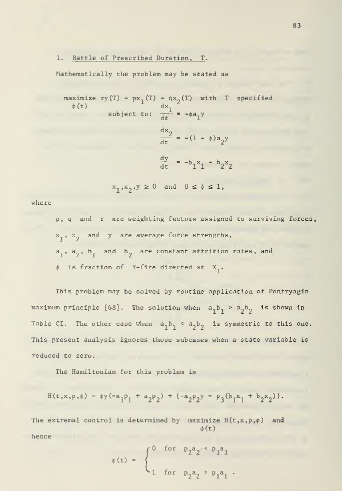
83

1. Battle of Prescribed Duration, T .

Mathematically the problem may be stated as

maximize ry(T) - px.. (T) - qx (T) with T specified4>(t) dx

±subject to: -z— = -<}>a y

dx

it ""b

lXl

" b2X2

x ,x ,y ^ and £ <|> £ 1

,

where

p, q and r are weighting factors assigned to surviving forces,

x , x and y are average force strengths,

a.. , a , b and b_ are constant attrition rates, and

<j> is fraction of Y-fire directed at X .

This problem may be solved by routine application of Pontryagin

maximum principle [68] . The solution when ^-.h, > a b is shown in

Table CI. The other case when a..b < a b„ is symmetric to this one.

This present analysis ignores those subcases when a state variable is

reduced to zero.

The Hamiltonian for this problem is

H(t,x,p,c{>) = t()y(-a1P1+ a^) + {-a^y - P

3(b

1x

;L

+ b^)}.

The extremal control is determined by maximize H(t,x,p,<j>) and

(t)

hence

<KO

rfor p -.< p^

1 f°r P2a2

>Piai

'

84

co•H•MCO

u

QT3CD

XI•H)-i

CJ

CO

CD

4-1

o

CO

pa

gCD

rH

O

Pm

Co•Huu0)

rH0)

C/l

4J

CD

60>-l

co

HOUCo

OCO

CD

CO

H

O

4-»

cou

1•H4J

D.O

HVI

4-1

VI

o

Mo

HA

o

HVI

•u

VI

o

uo

oII

/—n4-1

^^-e-

HV

uoM-l

t-

I

HVI

4-J

VI

o

uo

4-1

-e-

HVI

4J

VI

r-

I

H

l-i

O

OII

/—V4-1

-e-

cO

A

I-

CO

co•H4-1

Ico

CO

CO

CO

CO

crCN

CO

crCN

CO

A V

CO

aCO

PQ

OII

H

II

H

>

co•H4-J

CO

3cra;

co

4J

cCD

x)C0)

oCO

CcO

u

CD

x:4-1

so

T3CD

CHB

cu4J

QJ

T3

aCN

iO

I

cr

CM

CO

I

r~

43r-

cfl

CO

oCJ

cu CD

CO CO

cO cO

a c_>

o

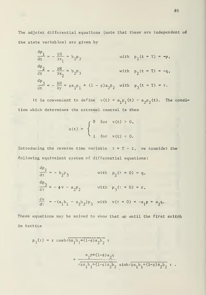
85

The adjoint differential equations (note that these are independent of

the state variables) are given by

dpl 3H

= b.p Q with Pl (t = T) = -p,dt 3x l

r3

Kl

dT= "i^ = b

2P3

With P2(t = T) = -

q '

dt= "

3

=Ct' a

lPl+ (1 ~ * )a2

P2

With P3(t = T) = r '

It is convenient to define v(t) = a p (t) - a p (t) . The condi-

tion which determines the extremal control is then

/ for v(t) > 0,

(t) =j^ 1 for v(t) < 0.

Introducing the reverse time variable x = T - t, we consider the

following equivalent system of differential equations:

dp2

= - b p with p (x = 0) = q,di "2 r3

""" K2

dp3

= - <J>v - a p with p (x = 0) = r,

— = "(a-^D-L- a

2b 2^P3 with V ^ T = °) = -a^ + a

2q.

These equations may be solved to show that up until the first switch

in tactics

p (x) = r cosh/^a-b +(l-<j>)a b_ x

a p+(H)a q+

•<|)a1b1+(l-<|))a

2b sinh/<|>a b +(l-<J>)a

2b x

86

It is easy to show that p (x), p„(x) < and p (x) > for all

x > 0.

We see that consideration of the case a -,b-i > a9

t»9

is motivated

by the coefficient of p,,(x) in the differential equation for v(x).

There are two further cases to consider.

Case (a) a p > a q

We have that <J>(t = 0) = 1> since v(x = 0) < 0. Now since

p (t) > 0, we always have -=— < and v(x) never can change sign.

Thus, we never switch. Hence, for £ t £ T, we have 4>(t) = 1.

Case (b) a p < a q

We have that <)>(t = 0) = 0, since v(x = 0) > 0. Since p„(x) > 0,

dvwe always have — < 0, and we can have a switch in tactics,

dx

The backward time of this switch in tactics, x = T, , is deter-. 1

mined from the integration of

f*= -(albl - a

2b2)p

3for * x * x^

where it is recalled that <J>(x) = in this interval. It is easily

shown that

ralblq

v(x) = -(a b -a b ){———- sinh/a b x + rf- cosh /a b x} - a p + —-— .

/a2b2

2 2

Thus, we determine x, from the transcendental equation v(x = t ^) = 0,

and the result shown in Table CI is obtained.

It is seen that for the battle of prescribed duration target

selection depends only on the attrition rates of the various force types

and relative weights assigned to surviving force types. For this model,

87

target selection is independent of force levels. This is not surprising,

since the adjoint differential equations are independent of the state

variables and the values of the dual variables at the end of battle

t = T are independent of force strengths. It is recalled that a dual

variable represents the rate of change of the payoff with respect to a

particular state variable [12]. Thus, if V = ry(T) - px (T) - qx?(T),

9Vthen p (T) = -— (t) , etc. Hence the boundary conditions are given for

the dual variables at the end of the battle t = T as p (t = T) =

— (t = T) = -p,P2(t = T) = -q,p

3(t = T) = r.

It seems appropriate to discuss further the interpretation of

the solution shown in Table CI. From the above definition of the dual

variables,

alPl (t) =return per unit time^ (kill rate of Y^ ^return per unit

for engaging X against X1

xof X destroyed

Hence, the condition a..p < a„q means that at the end of the battle

(recall that p (t = T) = -p , etc.) there is greater payoff per unit

time per soldier for Y to engage X (short term gain at the end of

battle). The value of the dual variable, for example, P-, (T) also

accounts for the effectiveness of X.. against Y. The condition

a b > a b may be interpreted to mean that there is more long range

return for engaging X . Thus, case A of Table CI corresponds to where

there is both more long range and also short range return for engaging

X.. . Case B corresponds to more short term gain at the end of the battle

for engaging X„ , but more long range return for engaging X.. . When

remaining forces at t = T are weighted proportional to their kill rates

88

against Y, i.e., p/q = b../b9

, then case A is the only one possible.

A switch in tactics (target priority) is seen to occur for this model

when more utility is assigned to survivors of a target-type than in

proportion to their destructive capability (kill rate) per unit relative

to other target types.

The maximum principle may be interpreted as saying that a target

type from several alternatives is engaged when such an engagement

yields the greatest marginal return. It turns out, though, that the

marginal value of target engagement evolves differently for different

model forms. This is clearly seen when we examine the solution for a

"fight to the finish."

2. Fight to the Finish .

We consider the similar problem of

maximize ry(T) - px (T) - qx„(T) with T unspecified

00dx

isubject to: -— = -<t>a y

dx

dT= - (1 -

*>V

£ = -bfi - b2x2

x- ,x >y ^ , £ $ <; 1 ,

and with terminal states defined by (1) x (T) = x (T) = and (2)

y(T) = 0.

The terminal surface of this problem is seen to consist of five

parts

:

89

C1

: X;L (T)- 0, x

2(T) > 0, y(T) - 0,

C2

:X;L (T)

= before x^T) = 0, y(T) > 0,

C3

:X;L (T)

- after x2(T) = 0, y(T) > 0,

C4

: X;L (T) > 0, x2(T) = 0, y(T) = 0,

C5

: xx(T) > 0, x

2(T) > 0, y(T) = 0.

The above problem was first studied by Isbell and Marlow [52],

and we develop its solution in detail in Appendix A. The solution to

this problem when a-ib-, > a b is shown in Table AI.

In contrast to the battle of prescribed duration, it is seen

that optimal target engagement may depend on initial force levels. When

Y wins, he engages X until depletion before X_ . When Y loses,

he may switch from firing at X entirely to firing at X entirely

before the X.. force has been annihilated. This happens when survivors

of force-type X are assigned utility in excess of their kill rate

as compared with force-type X- , and certain relationships hold between

initial force strengths. This dependence of the optimal allocation on

initial strengths has been caused by the fact that values of dual vari*-

ables at t = T are dependent upon values of the state variables.

This happens in terminal control attrition problems where a value of

a state variable is specified at the terminal surface (and hence the

value of the corresponding dual variable is unspecified but may be

determined from the transversality condition H(t = T,x,p,<|)) = 0).

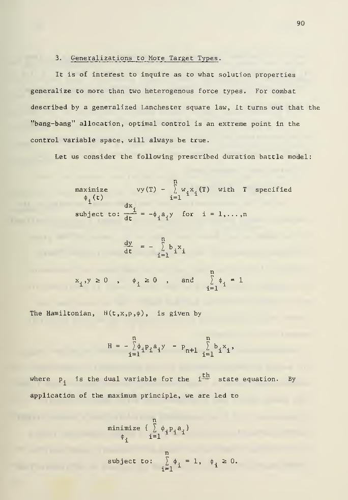
90

3. Generalizations to More Target Types .

It is of interest to inquire as to what solution properties

generalize to more than two heterogenous force types. For combat

described by a generalized Lanchester square law, it turns out that the

"bang-bang" allocation, optimal control is an extreme point in the

control variable space, will always be true.

Let us consider the following prescribed duration battle model:

n

maximize vy(T) - [ w.x.(T) with T specified

*. (t) i=lX X

dx.

subject to: -— = -tb.a.y for i = l,...,nJ dt i 3/

A n

dt,

L. l i

i=l

n

,y ^ , <}> 2> , and \ <f>= 1

i=l

The Hamiltonian, H(t ,x,p ,<))) , is given by

n nH = -y<j>.p.a.y -p., Tb.x.,

.

^n i l l rn+l .

L.. l l

i=l i=l

where p. is the dual variable for the i— state equation. By

application of the maximum principle, we are led to

minimize { \ <J) . p . a .

}

4>. i=l

n

4 .ill

n

isubject to: £ <J>

. = 1 ,<f>

. ^ 0.

i=l

91

Let i be the index such that a. p. = minimum (a,p,,...,a p ). ThenJ J 11 irn

<j>. = &.., where 5.. is the Kroncecker delta and is equal to 1 fori ij ij

i = j and is equal to otherwise, and all fire is concentrated on

one target type.

It is of interest to ask whether the optimal tactic will always

be to concentrate fire on only one target type (bang-bang optimal

control). The answer to this question turns out to be "no" as the

following simple example shows.

4. Linear Law Allocation .

So far the state equations have described combat according to the

Lanchester square law in which attrition of a target type is proportional

to the number of each force type firing at it. Weiss [81] has given

a thorough discussion of the conditions which lead to this. These

conditions include that "each unit is informed about the location of

the remaining opposing units so that when a target is destroyed, fire

may be immediately shifted to a new target." It is noted that the

control theory models which we have considered so far have implicitly

assumed perfect information.

Another model for attrition is the Lanchester linear law in which

the average decrease of a target type is proportional to the product

of the average number of targets remaining and the number of each force

type firing at it. Such a dependence can arise under two general

circumstances: (1) fire is uniformly distributed over a constant target

area ("area fire") or (2) the mean time of target acquisition is much

larger than target destruction time and is inversely proportional to

target density. The first circumstance corresponds to the simplest case

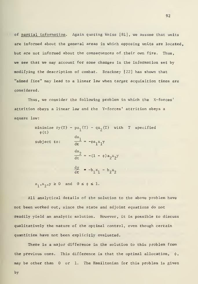
92

of partial information . Again quoting Weiss [81], we assume that units

are informed about the general areas in which opposing units are located,

but are not informed about the consequences of their own fire. Thus,

we see that we may account for some changes in the information set by

modifying the description of combat. Brackney [22] has shown that

"aimed fire" may lead to a linear law when target acquisition times are

considered.

Thus, we consider the following problem in which the X-forces'

attrition obeys a linear law and the Y-forces' attrition obeys a

square law:

minimize ry(T) - px (T) - qx (T) with T specified

<Kt)dx

lsubject to: -r—- = -<j>a..x y

dx2

dT= " (1 " * )a2V

f*= -b^ - b

2x2

x ,x ,y ^ and £<J>£ 1.

All analytical details of the solution to the above problem have

not been worked out, since the state and adjoint equations do not

readily yield an analytic solution. However, it is possible to discuss

qualitatively the nature of the optimal control, even though certain

quantities have not been explicitly evaluated.

There is a major difference in the solution to this problem from

the previous ones. This difference is that the optimal allocation, $,

may be other than or 1. The Hamiltonian for this problem is given

by

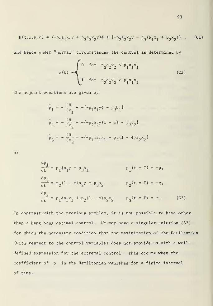
93

H(t,x,p,<j>) = (-p1a1x1y + p^x^H + {-p

2a2x2y - P^b-^ + b^)} , (CI)

and hence under "normal" circumstances the control is determined by

for P2a2*2

< P1a1x1

(C2)

1 for p2a2x2

> PlalXl

The adjoint equations are given by

PX - - "8^ - -{"PiV* " P3bl

}

p2

- -|~'- -{-p2a2yd - ) - p

3VP3

= -|f— -{-P^ " P2(l " *)a

2x2

}

or

dp,

p^a.y + p Qb np.(t = T) - -p

,

dt ri*-i-> r3-i fi

dp2— = p

2(l - <(>)a

2y + p

3b2

p2(t = T) = -q,

dp3

= p^a-x. + p_(l - <j>)a x o p„(t = T) = r, (C3)dt *-l

T*-l"l ^2 V T/-

2"2 r3

In contrast with the previous problem, it is now possible to have other

than a bang-bang optimal control. We may have a singular solution [53]

for which the necessary condition that the maximization of the Hamiltonian

(with respect to the control variable) does not provide us with a well-

defined expression for the extremal control. This occurs when the

coefficient of <j> in the Hamiltonian vanishes for a finite interval

of time.

94

A singular extremal is determined from the conditions [54]

9H n a d

if=

° andIt"

3H

3cj>

=

Hence, the following conditions must hold on a singular surface:

PlalXl

=P2a2X2

and alblXl

= a2b2X 2' (C4)

On the singular surface, the extremal control is given by

al+ a

2

(C5)

It may also be shown that such a singular control is impossible for

problems al and a2 . Thus, singular control (non-concentration of fire

on only one target type) is impossible for Lanchester square law

attrition but does play a central role in allocation when attrition

follows a linear law.

We must test to see if this singular solution can yield the

optimal return. A necessary condition for a singular subarc to yield

the maximum return [57] is

l_/ d

3c}> "dt2

"3H

3<j>

} ^ 0,

A rather laborious computation shows that

_3_(d 2

a<}> dt 73H

9<j>

} = y2p3(t){(a

1)2b

1x1+ (a

2)2b

2x2),

8 d 2and hence for p (t) > 0, we have that tt{^-7

3 di> dt

9H

3<f>,

} > 0. Thus, since

it may be shown that p^(t) > always, the necessary condition is

met for the singular path to be optimal.

95

In constructing the extremal trajectories and tracing the optimal

course of battle (backwards from the end of the prescribed duration

battle) it is convenient to introduce

v(t) = -a1P1x1+ a

2P2x2

, (C6)

then

dvdp

ldx

ldp

2dx

2

dF= "a

i dT xi

" aipi IT + a

2 dT X2+ a

2P2 dT

Using the state equations and the adjoint equations (C3) , we obtain

from the above

aT= " (a

2b2X2

" aiblXl)p 3'

or, in terms of the backwards time t = T - t, this becomes

oT= (a

2b2X2

" alblXl)p

3(C7)

We may write (C6) as

v(x) = -,b2 ]

Px(t)

Ip 2(t)J

"bTT alblXl

" a2b2X2

b2

(C8)

We note that (C2) and (C6) may be combined to yield the non-singular

control

4>(t) =

1 for v(t) >

for v(t) < 0, (C9)

and the singular control is

2<j)(t) = for v(t) 0,

a _ *T" cL r

(CIO)

96

when the system is in the state described by (C4).

We note that at the end of battle x = 0, we have

v(t = 0) = -alPXl (t = T) + a2qx

2(t = T)

.

(Cll)

If we were to consider in Figure CI the line L' defined by a px =

a_qx9

, then it would appear above, on, or below the line L defined

by a.-b-x = a b„x depending on whether -^ were greater than, equal

to, or less than

these two lines

This is evident from considering the slopes of

dx.

dx,^1a2b2

'

dx.

dx

aiP

a2q

' L'l

and hence, for example,

dx/flx -\

ldxiJ

*- T I

dx/-ax^

Mvfor ^>^.

q b2

The significance of the line L' and its relationship to the line L

is that

v(x = 0) '

' > below L 1

^ < above L'

,

(C12)

and hence by (C9) we find that

1 for P(T) below L'

<J>(t = T) =

/ 1 fo

v fo r P(T) above L'

,

(C13)

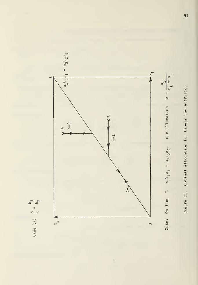
cn

CN

CN

97

x> ^

cM cr

CM

cO

+

CM

CN

I—

o

Go•H•u•H!-i

4-1

4-1

g

}-i

CO

G

o•H4JCO

CJ

o

cO

E•rH

4-1

D-O

U

J-4

GO•H

0)

cn

cO

CJ

CD4-1

O

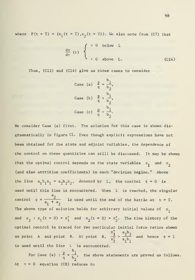
98

where P(t = T) = (x (t = T) ,x (t = T) ) . We also note from (C7) that

dv( s

di

> below L

< above L. (C14)

Thus, (C12) and (C14) give us three cases to consider

b

Case (a) £ = 7^,q b

2

b

Case (b) £ > —-,q t>

2

bx

Case (c) -^ < 7—.q b

2

We consider Case (a) first. The solution for this case is shown dia-

grammatically in Figure CI. Even though explicit expressions have not

been obtained for the state and adjoint variables, the dependence of

the control on these quantities can still be discussed. It may be shown

that the optimal control depends on the state variables x and x„

(and also attrition coefficients) in each "decision region." Above

the line a b x = a b x , denoted by L, the control<J)

= is

used until this line is encountered. When L is reached, the singulara2

control c}> = ; is used until the end of the battle at t = T.a1+ a

2

The above type of solution holds for arbitrary initial values of x..

and x : x (t = 0) = x° and x (t = 0) = x°. The time history of the

optimal control is traced for two particular initial force ratios shownXl

a2b2

as point A and point B. At point B, —5- > —:— and hence cf>

= 1x2

albl

is used until the line L is encountered.bl

For Case (a) :^ = :— , the above statements are proved as follows,q b

2

At t = equation (C8) reduces to

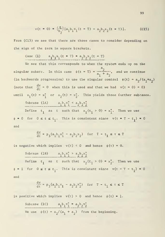
99

v(x = 0) = (^-)[a1b1x1(t = T) - a

2b2x2(t = T) ] . (C15)

From (C15) we see that there are three cases to consider depending on

the sign of the term in square brackets.

Case (1) a1b1x1

( t " T) - a^x^t = T)

We see that this corresponds to when the system ends up on the

a2

singular subarc. In this case <J>(t = T) = —, and we continue

al

a2

(in backwards progression) to use the singular control (f>(t) = a9/(a,+a_)

(note that — = when this is used and that we had v(t = 0) = 0)dx

until x (t) = x° or x (t) = x° . This yields three further subcases.

Subcase (1A) a-.b-.xf' < a9b_x°

Define t.. as t such that x (t > 0) = x°. Then we use

<})= for £ t £ t . This is consistent since v(x = T-t)=0

and

~ = p (a1b

1x° - a„b x ) for T - t, £ x <; T

C1T Jill III 1

is negative which implies v(x) < and hence $(t) = 0.

Subcase (IB) a b x° > a b x°

Define t.. as t such that x ^( t->

> 0) = x o- Then we use

$ = 1 for j* t s: t.. . This is consistent since v(x - T - t ) =

and

a7= P

3(a

1b1x1

- a2b2x°) for T - t

±Z x S T

is positive which implies v(x) > and hence cj)(x) = 1.

Subcase (1C) a b x° = a b x°

We use <)>(t) - ao/(a T+ a

9) from the beginning.

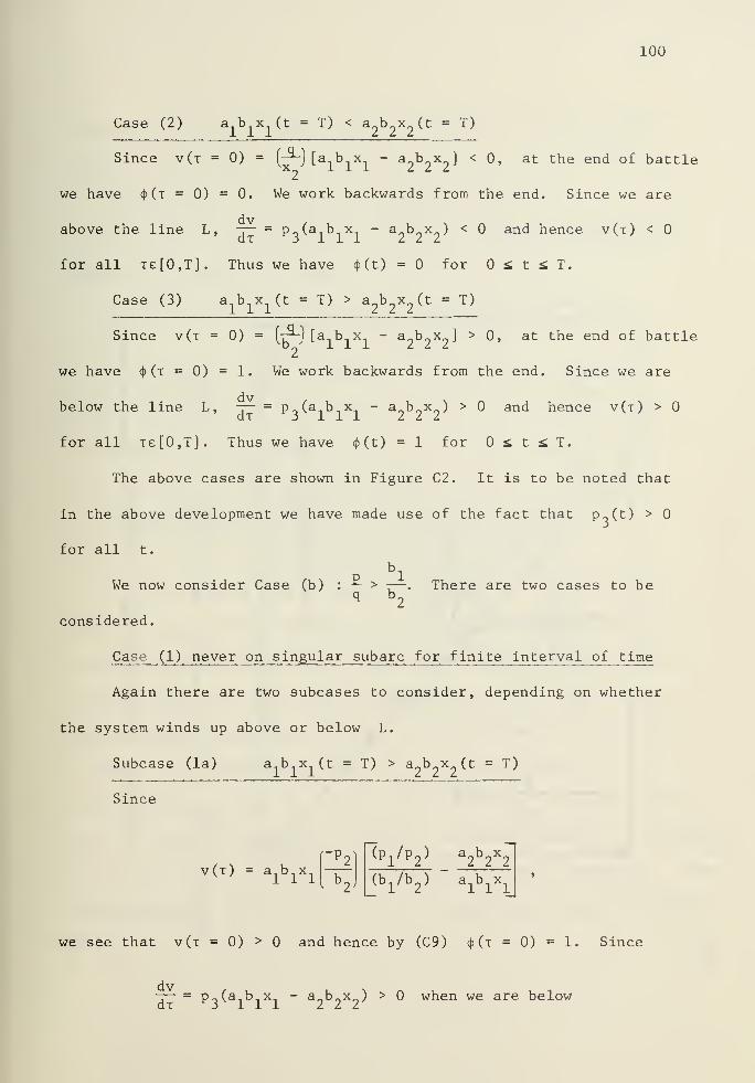
100

Case (2) a.b x (t = T) < a b2x (t = T)

Since v(t = 0) = (-^-) [a b x - a b x ] < 0, at the end of battle

we have 4>(t = 0) = 0. We work backwards from the end. Since we are

above the line L, — = p„(a1 b 1 x. - a.b_x_) < and hence v(t) <

dx Jill Z Z Z

for all xe[0,T]. Thus we have <j>(t) = for £ t <. T.

Case (3) a b^ (t = T) > a b x2(t = T)

Since v(x = 0) = (^[a.Lx, - a_b^x_] > 0, at the end of battlet>9

111 Z Z Z

we have <j)(x = 0) = 1. We work backwards from the end. Since we are

below the line L, — = p„(a 1 b.x 1- a.b_x„) > and hence v(x) >

dx Jill 2 2 Z

for all xe[0,T]. Thus we have <j>(t) = 1 for <; t £ T.

The above cases are shown in Figure C2. It is to be noted that

in the above development we have made use of the fact that Po(t) >

for all t.

b

We now consider Case (b) :^- > -—

. There are two cases to beq b

2

considered.

Case (1) never on singular subarc for finite interval of time

Again there are two subcases to consider, depending on whether

the system winds up above or below L.

Subcase (la) aiblXl(t = T) > a

2b2x2(t = T)

Since

v(x) = a-jb.^r-p- (P

1/P

2 >a2b2X2

(b1/b

2) a

1bixi

we see that v(x = 0) > and hence by (C9) <j>(x = 0) = 1. Since

— = p„(a b x - a b„x ) > when we are below

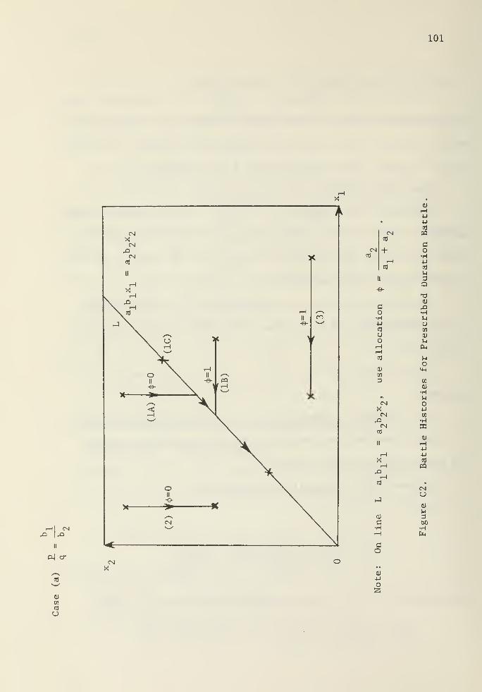
101

CN

o| cr

wco

u

CN

CN PQccj

CM + o

•HrH 4-J

cd CO

l-i

II 3Q

-e-"00)

C XIo •H•H >-i

•U Uco CO

o 0)

o ^H PLirHcO M

oQJ >4-|

w3 0)

w•H

A uCNX 4-1

CM Cfl

XI •i-l

CN Xco

0)

II H4-J

H 4-1

X COH PQXHCO •

CNU

hJ0)

u<U 3e bO•H •r-l

H |i<

CO

CD

4J

O2

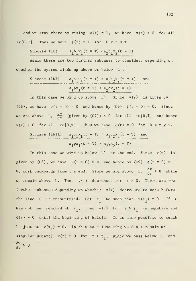
102

L and we stay there by rising <Kt) =1, we have v(t) > for all

te[0,T]. Thus we have <t>(t) = 1 for £ t si T.

Subcase (lb) a b x (t = T) < a b x (t = T)

Again there are two further subcases to consider, depending on

whether the system winds up above or below L'.

Subcase (lbl) a b x (t = T) < a b x (t = T) and

a1px

1(t = T) < a

2qx

2(t = T)

In this case we wind up above L' . Since v(t) is given by

(C6), we have v(x = 0) < and hence by (C9) $ (x =0) =0. Since

we are above L, — (given by (C7)) < for all xe[0,T] and henceax

v(t) < for all xe[0,T]. Thus we have cj>(t) = for S t i T.

Subcase (lbll) a b x (t = T) < a b x (t = T) and

a1px

1(t = T) > a

2qx

2(t = T)

In this case we wind up below L' at the end. Since v(x) is

given by (C6), we have v(x = 0) > and hence by (C9)<J>

(x =0) = 1.

dvWe work backwards from the end. Since we are above L, -7— < while

dx

we remain above L. Thus v(x) decreases for x > 0. There are two

further subcases depending on whether v(x) decreases to zero before

the line L is encountered. Let x be such that v(x ) =0. If L

has not been reached at x.. , then v(x) for x > x- is negative and

<\>(t) = until the beginning of battle. It is also possible to reach

L just at v(x..) = 0. In this case (assuming we don't remain on

singular subarc) v(x) > for x > x.. , since we pass below L and

dx

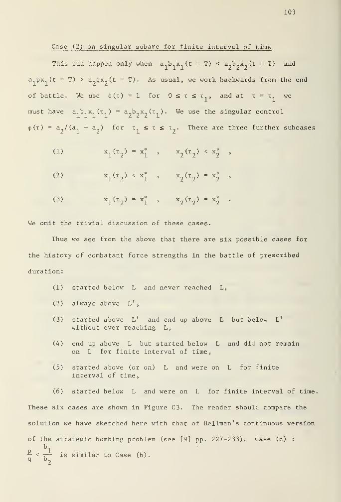
103

Case (2) on singular subarc for finite interval of time

This can happen only when a b x (t = T) < a_b x (t = T) and

a px (t = T) > a qx (t = T) . As usual, we work backwards from the end

of battle. We use 4>(t) = 1 for £ t £ t1

, and at T = T1

we

must have a..b..x (t.) = a„b x9(t,). We use the singular control

4>(t) = a / (a + a ) for t, £ t £ t . There are three further subcases

(1) X1^ T2')

= Xl '

x2

( T 2-) < x2 '

(2) x (t2

) < x°,

X2

(- T 2^= X

2 '

(3) X1^ T 2^= X

l 'X2

( T 2')= x

2 '

We omit the trivial discussion of these cases.

Thus we see from the above that there are six possible cases for

the history of combatant force strengths in the battle of prescribed

duration

:

(1) started below L and never reached L,

(2) always above L'

,

(3) started above L' and end up above L but below L'

without ever reaching L,

(4) end up above L but started below L and did not remainon L for finite interval of time,

(5) started above (or on) L and were on L for finiteinterval of time,

(6) started below L and were on L for finite interval of time.

These six cases are shown in Figure C3. The reader should compare the

solution we have sketched here with that of Bellman's continuous version

of the strategic bombing problem (see [9] pp. 227-233). Case (c) :

bl

-^ < r— is similar to Case (b) .

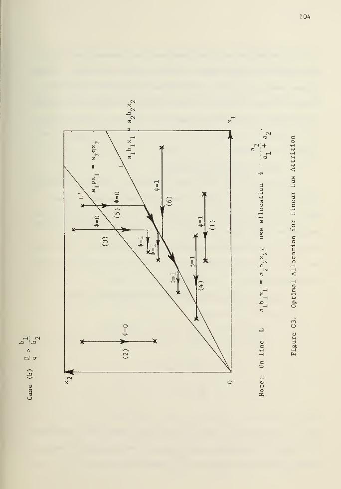
CN

104

r-l CM

A

wcd

cd Co

+ •1-1

4-1

--H •HCd >-i

4-1

II 4-1

-^.<£cd

c JoH ^4-1 cd

cd <u

o Ci

O •HhJ

CO uo

0) U-l

V)

3 eo•H

** 4J

CM cd

X oCNl o

rO r-H

CM .-1

cd <d

II rHcd

.H BX •H-H 4J

X (X.H o

CO

C~)

UJ

<U

)-i

0) 3c 00•H •T-l

rH to

co

QJ

Uo!3

105

The reader's attention is directed to the interpretation of these

three cases. Case (a) is when Y assigns utility to surviving X-force

types in exact proportion to their destructive capability against Y.

Case (b) is when Y assigns a greater utility to surviving X ' s than

in proportion to their kill rate against Y relative to that of X .

It is recalled that similar type remarks were made with respect to the

solution of problem al.

b . Effect of Resource Constraints .

In this section we will examine a sequence of models of increasing

complexity for which the effect of ammunition limitations on firing

rate (fire discipline) will be explored. In each case, we consider two

homogeneous forces engaged in combat described by a square law. The

research on these models has not progressed as far as that on the earlier

ones. For some of these models the results are of a preliminary nature,

the entire solution not having been completely worked out.

1. Battle of Prescribed Duration with Constant Kill Rates .

We consider the situation

maximize px(T) - qy(T) with T specified

*< C > dxsubject to: — = -a.

y

J dt lJ

dt= ~* Va

2X

dz a

z,y 2t 0, £<f>

s: 1, z(t = 0) = 0, and z(t = T) £ A < vT = v dt,

where v is the maximum firing rate of each X unit. It is noted that

the nature of the attrition coefficients a| and a is different,

since a., has incorporated in it a constant firing rate.

106

This corresponds to the case where each X combatant has a limited

supply of ammunition, denoted by A. We assume that this supply is such

that he could not fire at his maximum firing rate for the prescribed

duration of the battle, for when A ^ vT it is easily seen that the

optimal strategy is to fire at the maximum possible rate, <$>(t) = 1

for £ t £ T.

The optimal regulation of firing rate turns out to be

A

4>(t) = 1 for £ t £ T where T =1 v

(t) = for T £ t £ T.

This was determined as follows. The Hamiltonian is given by

H(t,x,p,<})) = <f>v(p3

" P2a2x ) " p

iaiy >

and hence

=

for p < P2a2x

for p3

> P^x.

The adjoint differential equations are given by

Px- - -^ - <l>va

2p2

with px(t = T) = p

P2

= " 9y"= a

lPl

Wlth P2(t = T) = _q

p (t) = const.

We introduce the reverse time variable t = T - t and consider a

backwards integration of the state and dual variables from the fixeddp

lend of the battle, t = T. Hence, -— = -<bva„p_, etc. It is easy

QT 11

107

to show that p (t), x(t), and yd) are non-decreasing functions

of t (regardless of <J>) with p 1(x = 0) = p, x(t = 0) - x , and

1 s

y(r = 0) = y . Similarly, p„(x) is a strictly decreasing function

of t. Hence, Q(t) = a p (t)x(t) is a strictly decreasing function

of x with an initial value of Q(t = 0) = -qa x . Thus, p must

be negative, and <Kt) never switches back to once it becomes 1.

This solution is distrubing, since it is not intuitively appealing

to fire at one's maximum firing rate until one runs out of ammunition

and to spend the final stages of battle without ammunition. Hence, we

are led to consider other models for further insight.

2. Battle of Prescribed Duration with Time Varying Kill Rates.

We consider the situation

maximize px(T) - qy(T) with T specified

<t>(t)

dx , ssubject to: — = -a (t)y

dy / s

-j£ = -(|>va (t)x

dzA

dT=

* v

x,y ;> 0, Osf si, z(t = 0) = 0, and z(t = T) s A < uT,

It seems reasonable to assume that in mnay real world situations a (t)

and a„(t) would be monotonically increasing functions of time, e.g.,

two forces closing with each other. All the previous solution steps

remain the same except for the effect of a., (t) and a (t) increasing

with time. This may change the solution markedly, although the optimal

control is still bang-bang. The quantity Q(t) = a9(t )p ?

(t)x(t) is

not guaranteed to be a strictly decreasing function of t, since a (x)

108

is strictly decreasing (but positive) and P 9(t) is negative. This

allows the possibility that the optimal tactic may be to hold one's

fire and conserve ammunition in the early stages of battle so that

4>(t = T) = 1 at the end of battle.

The way in which ammunition is conserved depends on the specific

nature of a (t) and a_(t). It seems worthwhile to explore optimal

tactics for several simple time dependencies of these quantities, but

this hasn't been done as yet. We would recommend that this be a future

research task. In Appendix D, we develop the solution to variable

coefficient (either force separation or time as the independent variable)

Lanchester-type equations when the ratio of attrition rates is a constant,

This allows an analytic solution to be obtained for the problem at hand

in special instances. It is not unreasonable to expect to encounter

cases in which one holds his fire until the kill probability reaches

some threshold value. An aspect that is disturbing is that the control

has turned out to be bang-bang. One can show, in fact, that a singular

solution is impossible for this problem.

R. Isaacs has studied some similar problems in his book Differen-

tial Games [50] and has explored some aspects of this problem much deeper

than presented here. Isaacs tried to resolve the problem of shooting

up all of one's ammunition before the end of the battle by modifying

the payoff. Another approach might be to consider a terminal control

problem.

3. Fight to the Finish with Limited Ammunition .

Thus we are led to consider

maximize px(T) - qy(T) with T unspecified4>(t)

109

subject todx

dt- -a

l7

dt= -<j>va x

dz

dt= <J>v

x,y ^ 0, £ <j> £ 1, z(t = 0), and z(t = T) £ A,

with terminal states defined by (1) x(T) = and (2) y(T) = 0.

We briefly consider the constant attrition coefficient case, although

it is noted that a similar analysis would apply to time dependent

attrition coefficients. As with the previous terminal control problem,

dual variables (marginal gains) now are related to the final values

of the state variables by virtue of H(t,x,p,<}>) = const. = =

H(t = T,x,p,c}>). We might encounter a case where tactics are dependent

on enemy force level (in the previous limited ammunition cases, tactics

are independent of enemy force level), but this case has not yet been

explored very far.

One point worth noting is that for the constant attrition coeffi-r

cient case the X forces in order to win are required to have enough

ammunition to fire at their maximum rate during the entire duration of

the battle. Hence, we see that concentration of forces reduces the

ammunition requirement per man, since the length of battle is determined

by initial numbers of forces committed to battle.

4 . Two-Sided Extension .

There appears to be a novel feature in a two-sided version of the

above problems. Again, we briefly make a few remarks about the constant

attrition coefficient case.

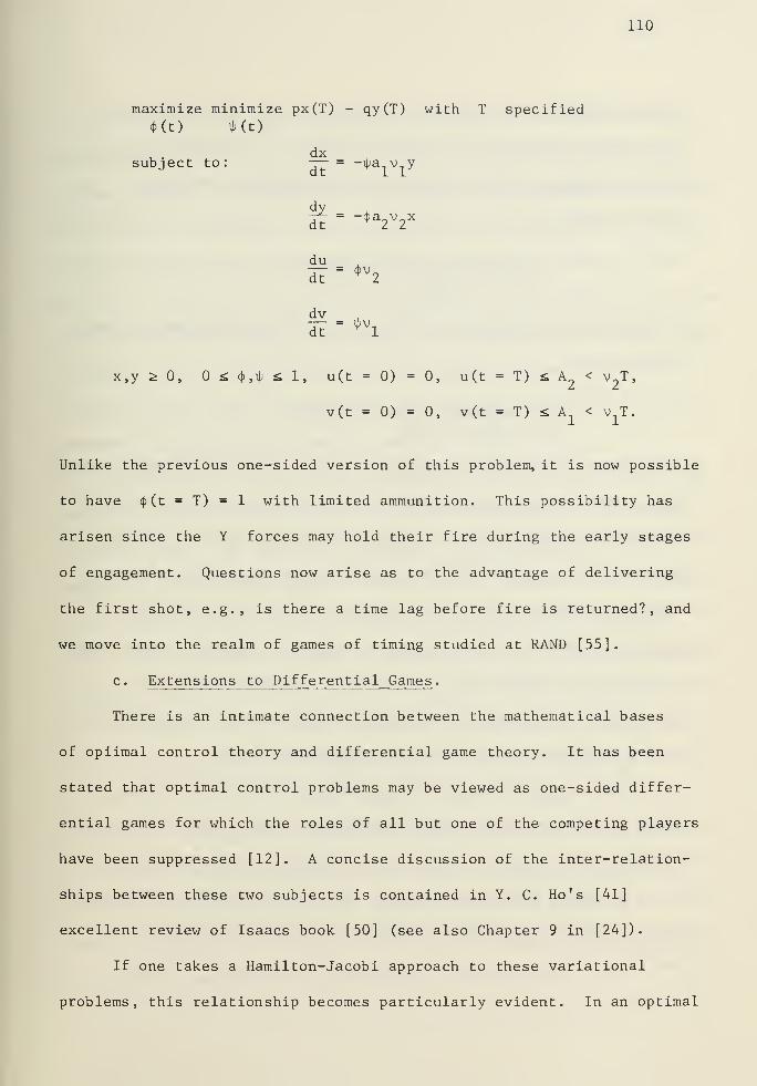
110

maximize minimize px(T) - qy(T) with T specified

subiect to: ~r- - -iiia,v,ydt 11

dT= "* a

2V2X

dUA

dt~=

* V2

dvdT

=* v i

x,y ;> 0, s£ <$>,\p £ 1, u(t = 0) = 0, u(t = T) <; A < v T,

v(t = 0) = 0, v(t = T) <: A < v T.

Unlike the previous one-sided version of this problem, it is now possible

to have <J>(t = T) = 1 with limited ammunition. This possibility has

arisen since the Y forces may hold their fire during the early stages

of engagement. Questions now arise as to the advantage of delivering

the first shot, e.g., is there a time lag before fire is returned?, and

we move into the realm of games of timing studied at RAND [55].

c. Extensions to Differential Games .

There is an intimate connection between the mathematical bases

of opiimal control theory and differential game theory. It has been

stated that optimal control problems may be viewed as one-sided differ-

ential games for which the roles of all but one of the competing players

have been suppressed [12]. A concise discussion of the inter-relation-

ships between these two subjects is contained in Y. C. Ho's [41]

excellent review of Isaacs book [50] (see also Chapter 9 in [24]).

If one takes a Hamilton-Jacob i approach to these variational

problems, this relationship becomes particularly evident. In an optimal

Ill

control problem we are seeking the solution to the following partial

differentail equation for the optimal return, S (referred to as

Hamilton's characteristic function in the calculus of variations

literature [69]),

3S• „/ as xN— + maximum H(t ,x,— , <J>)

= 0,dt

, / \ oX<j)(t)

with appropriate boundary conditions. In a differential game we seek

the solution to

3 S 3 SJ- maximum minimum H(t ,x,— ;<|> ,ip) = 0.

3t4>(t) *<t)

9X

It also seems appropriate to mention the relationship of dynamic program-

ming to these techniques. Consideration of the equation satisfied by

the optimal return points out clearly an important aspect of dynamic

programming, its being a discrete approximation technique for solving

variational problems [30]. It is, however, a dual approach which

generates an optimal trajectory as an envelope of tangents rather than

as a sequence of points [10] . The value of the continuous models lies

in their ability to exhibit explicitly the dependence of optimal tactics

on model parameters rather than any computational ease.

It is noted that the existing theory for differential games

assumes that the optimal strategy (during any finite interval of time)

is always a pure strategy. Hence, it is necessary that max min H =

min max H almost everywhere in time. There are, however, differential

games of practical interest for which pure strategy solutions do not

exist [11].

112

In light of the above discussion, it is easy to see the value of

beginning the study of mathematical models of tactical allocation with

optimal control. It is true that actual combat is a competitive environ-

ment in which the actions of both parties must be considered, but optimal

control problems may be used to study most significant aspects of such

problems: setting proper boundary conditions, devising solution procedures,

study of singular solutions, differences in solutions for different forms

of model. Most solution aspects of the one-sided problem are present

in the two-sided one. It is assumed that formulation of these two-sided

problems is clear from the previous content of this paper.

Of interest to the operations research worker is whether there is

any new aspect of solution behavior in a differential game. The answer

to this is "yes." In devising a rigorous solution procedure for the

supporting weapon system game of H. K. Weiss [82], we have (see Appendix

B) encountered solution behavior unique to terminal control attrition

games: there may exist a domain of controllability for a given terminal

state but entry to this state may be "blockable" by the "losing" player.

In other words, there is a path determined by the necessary conditions

leading from each point in a region of the initial state space to a

terminal state, but the "losing" player may use a strategy other than

his extremal strategy for this path to actually win. In the process

of solving the supporting weapon system game and trying to understand

the many complicated facets of its solution procedure, we gained

insight by considering a related optimal control problem (see Appendix

A), the Isbell and Marlow fire programming problem [52].

113

d. Implications of Models .

It seems appropriate to briefly discuss the general implications

in the following areas of the models examined in this paper:

(1) optimal tactical allocation,

(2) intelligence,

(3) command and control systems,

(4) human decision making.

The discussion of these areas is not mutually exclusive.

Of interest to the military tactician is whether target selection

rules evolve dynamically during the course of battle. Are target

priorities static or do they evolve dynamically with the course of

battle? With respect to optimal control models, this may be mathemati-

cally stated as whether there are transition (switching) surfaces in

the solution. We have seen in the idealized and simplified models

studied here that target priorities do change. This is related to the

evolution of marginal return of target destruction (value of dual

variable) . We have seen that this evolution depends on the goals of

the combatants (utility assigned to surviving force types at the end

of the battle) and also the conditions which terminate the battle. In

the terminal control problem studied here, a shift in target priorities

is present only in a losing case, whereas in a fixed duration battle

such a switch is independent of winning or losing but depends only on

weapon system capabilities and the prescribed duration of battle.

Even though these models assume complete and instantaneous

information, it appears that some inferences may be made for cases

where uncertainty is present. In the terminal control case, we saw

114

that selection of tactics depends on a knowledge of the enemy's strength

and capabilities, since the terminal state of combat must be determined

before optimal strategies can be. For a battle of prescribed duration,

e.g., fighting a delaying action in a retrograde movement to protect

the withdrawal of troops, tactics depend only on enemy and friendly

capabilities and length of combat, not the initial force levels. For

such cases the estimate of combat length is critical, since changes in

target priorities are determined relative to the end of the engagement.

Schreiber [70] has proposed an idealized and simple, but yet

illuminating, way of quantitatively showing the value of intelligence

and command control capabilities. He introduces the concept of "command

efficiency," which is measured by the fraction of the enemy's destroyed

units from which fire has been redirected. The effect of poor intelli-

gence and poor capabilities for redirecting fire from destroyed targets

is to produce "overkill." Schreiber 's equations for combat involved

this fraction called "command efficiency," and they reduce to Lanchester-

type equations for area fire when the fraction is and aimed fire

for a value of 1. We have seen that the optimal tactics are quite

different for these two cases. When intelligence and command control

systems are very efficient, the optimal tactic is seen to be concentra-

tion of fire on a specific target type. When capability for redirection

of fire from destroyed targets is poor (either through damage assessment

or constraints on new target acquisition) , the optimal tactic may be

to allocate fire in a proportional fashion over target types in a way

that holds the ratios of target density in each target area to be

constant. Another implication is that supporting weapon systems (e.g f ,

115

artillery) concentrate fire on selected point targets, but that fire

is allocated proportionately over various area targets. Thus, these

models suggest that the tactics of target engagement may vary with

command and control capabilities.

These models also show the importance of intelligence in devising

the best tactics in combat. Intelligence on enemy weapon system

capabilities (kill rates including target acquisition rates) and poten-

tial length of engagement play a central part. We also have seen that

for fights to the finish and linear law attrition cases intelligence

on enemy force levels is also required. For artillery fire support

missions against various troop concentrations, knowledge of troop

densities is essential in the assignment of target priorities. Particu-

larly dense concentrations where the initial kill potential is high are

seen to be cases where the optimal tactic is to concentrate fire on one

target for awhile.

Another argument for the concentration of forces is seen to emerge

from the study of these simplified models. When ammunition is limited,

a concentration of forces has the effect of counter-balancing this

constraint. For example, in a fire fight numerical superiority could

mean that the enemy force level would be reduced such that he would

disengage in time before the friendly ammunition restriction became

critical.

These models may be interpreted to show the value of human judgment

in combat. They indicate, as does common sense and experience, that in

battle a commander must use his judgment to ascertain to what end can

the course of battle be steered so that he may devise his strategy

116

accordingly. The demonstrated sensitivity of these models to many

factors shows the importance of human assessment of a situation and

the importance of good judgment in assigning utility to forces surviving

the battle at hand.

e. Summary .

The results of this appendix may be summarized as follows:

(1) a sequence of one-sided models has been presented which showsthat the tactics of target selection may be sensitive to

force strengths, target acquisition process, the type of

attrition process, and/or the termination conditions of

combat

,

(2) a sequence of models have been presented which shows somepreliminary results on the effect of resource constraintson firing discipline and concentration of forces,

(3) tactics for target selection are heavily dependent upon"command efficiency,"

(4) concentration of fire on one target type among many occursas an optimal tactic only when target acquisition is notsubject to diminishing returns.

117

APPENDIX D. Solution to Variable Coefficient Lanchester-Type Equations.

In Appendix C, we briefly considered a model involving Lanchester-

type equations with variable coefficients. Although such equations

have been studied by analysts for over 10 years since H.Weiss' pioneering

work [81] , analytic solutions for the average force strengths (state

variables) as a function of an independent variable (either time or

range) have been obtained in only isolated instances [19], [20]. We

have discovered a very general method for solving such variable coeffi-

cient equations under certain assumptions about the average attrition

rates of the combatants. We point out, however, that all previously

published results [73] except one are contained in the general results

presented here. Additionally, these new results also apply to cases in

which the relative velocity of combatant forces is a function of force

separation.

We show how to solve Lanchester-type equations for combat between

two homogeneous forces when the attrition rates are variable provided

that their quotient is a constant. Solutions are developed for either

time or force separation as the independent variable. We also investi-

gate under what circumstances each of Bonder's two second order differential

equations [20] can be transformed into a constant coefficient equation

yielding exponential solutions. We begin by briefly reviewing previous

work on this topic.

H. Weiss [81] extended Lanchester-type equations to include the

relative movement of two homogeneous forces, allowing time and space

to be "traded" for casualties. He considered the two attrition rates

118

to be dependent upon force separation in such a way that their quotient

was a constant. S. Bonder [19], [20] and others [73] have used Weiss'

extension to study the effects of mobility and various range dependen-

cies of the average attrition rates on the number of surviving forces.

For each force type, he developed a second order differential equation

which related average force strength to the force separation, r, and

obtained solutions for cases of constant relative velocity of forces.

We show that more general results are easily obtainable by consid-

ering the original first order system of equations with either time or

force separation as the independent variable (as is appropriate for the

problem under study). Bonder's results [20] and the constant attrition

rate solution are but special instances of our more general results.

a. Range Dependent Attrition Rates .

The case of range dependent attrition rates originally motivated

this approach, although it is now seen to be a special case of time

dependent attrition rates. We use the same notation as Bonder [20], [73^

for the battlefield coordinates.

We consider

dx .

d7= -a(r)y

'

£--B<r)x.

where

a(r) a

B(r) " kfi

and x,y are average force strengths,

a(r),B(r) are average (range dependent) attrition rates,

119

Considering force separation, r, as the independent variable, we

dx dx , , , ,have -r— = v -r~ and thus the equations becomedt dr H

dx . _k Silly

dr a v(r) '

£L = _k &LLL x . (d1)dr 3 v(r)

We consider the relative velocity of the forces to be a function of

force separation only. As Weiss [81] has pointed out, these equations

readily yield a square law relationship between the state variables

kg(x 2 - xg) = k

a(y

2 - y 2). (D2)

Solving equation (D2) for y, substituting the result into the first

of equations (Dl) , and integrating from r = R and x = x to r

and x, we obtain

^ d- ™

Raising e to the power of each side of equation (D3) , we obtain the

following result after some algebraic manipulation:

x(r) = x cosh + y A. /k sinh 6,

U ot B

where

e(r) = -^Tkg

r

^\ du. (DA)v(u)

Ro

A similar expression is readily obtained for y(r). Bonder's [20]

results are special cases of equations (D4)

.

120

b. Time Dependent Attrition Rates .

More generally, we might be interested in

dx , , , .

d?= "k

Bh(t)x -

The same approach as above readily yields

x(t) = x_ cosh + y./k /k sinh

where

9(t) =-v^jt

h(u)du. (D5)

When h(t) = 1, equations (D5) reduce to the familiar constant coefficient

solution. When h(t) = g(r(t)) and r(t) = Rn + v(t)dt, equationsi

(D5) reduce to equations (D4).

c . Some Comments .

We see from the above that the effect of time (range) dependent

average attrition rates of the form considered is to transform the time

(range)scale of the usual square law attrition process. Thus we see

that certain time (range) intervals are weighted more heavily in the

transformed time (range) scale than they are in the usual square law

attrition process.

Previous analytic work [73] has assumed that the relative velocity

between forces to be constant. These results allow this restriction to

be relaxed. For example, we may now easily study combat situations in

which relative velocity is a decreasing function of force separation.

121

We would strongly recommend that the results developed here be

used in extensions of the allocation models developed in the previous

appendix. The approach developed here also applies to the solution of

the adjoint equations in the determination of our new dynamic kill

potential developed in Appendix F.

d. The Condition for Solution in Terms of Elementary Functions .

We discuss in this section necessary and sufficient conditions

for a second order ordinary differential equation which Bonder has

derived [20] to be transformed to a constant coefficient equation

yielding exponential solutions. This covers all but one of the results

obtained by Bonder [73].

We start by considering

dx

dr= a(r)

V y»

dy_

dr= 3(r)

Vx, (D6)

which is implicit in the development of (Dl). By differentiation and

substitution, we may combine these equations into a single second order

equation for x.

d^x d_f oCO] + a(rl dy_ = Qdr z dr (. v J v dr

or

d zx dx d / „ a(r)f a(r)g(r)d

2 x _ dx _d_/£n

q(r)| _ a(r)(

r^ dr dr I v / v'x = 0,

which for v = constant (i.e., constant relative velocity of force

movement) becomes

d 2x 1 da dx ag *

, 7 ,

T~I T~ ~T~ j x = 0. (D7)dr^ a dr dr v z

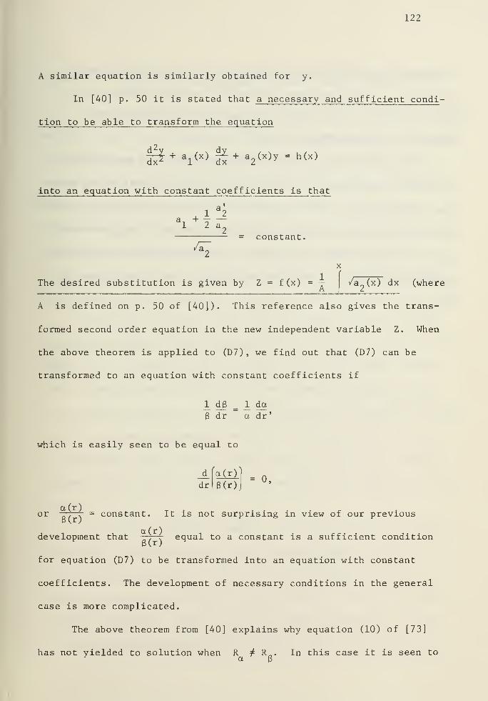
122

A similar equation is similarly obtained for y.

In [40] p. 50 it is stated that a necessary and sufficient condi -

tion to be able to transform the equation

P£ + a.(x) f- + a,(x)y = h(x)Ix*

1 1 dx 2

into an equation with constant coefficients is that

a + — —1 2 a

= constant.a2

The desired substitution is given by Z = f (x) =

x

1/a (x) dx (where

A is defined on p. 50 of [40]). This reference also gives the trans-

formed second order equation in the new independent variable Z. When

the above theorem is applied to (D7), we find out that (D7) can be

transformed to an equation with constant coefficients if

ldB = IdaB dr " a dr'

which is easily seen to be equal to

d fa(r)

dr 3(r)= 0,

or —,—r = constant. It is not surprising in view of our previous3(r) r v

development that n , s equal to a constant is a sufficient conditionB(r)

for equation (D7) to be transformed into an equation with constant

coefficients. The development of necessary conditions in the general

case is more complicated.

The above theorem from [40] explains why equation (10) of [73]

has not yielded to solution when R ^ R„. In this case it is seen toa 8

123

be impossible to transform the equation into one yielding exponential

solutions. Our work here then confirms the conjecture made in [73]

that the condition which facilitated the results obtained at the

University of Michigan was that , . = constant.6(r)

We also note that the transformations employed by Bonder [20]

are readily discovered by p. 50 of [40] but omit the details. We have

also briefly tried to solve equation (10) of [73] for R ^ R by classi-

cal ordinary differential equation methods (see [45] or pp. 530-576 of

[65]). It appears that this equation is not a standard form and series

methods must be used. Time has permitted only a very cursory look at

this.

124

APPENDIX E. Connection with Bellman 'a Stochastic Gold-Mining Problem .

In this appendix we solve several versions of a continuous stochastic

decision process by means of the Pontryagin maximum principle. The basic

problem has been called the continuous version of a stochastic gold-

mining process (see pp. 227-233 of [9]), but it is really an idealiza-

tion of an allocation problem for strategic bombers. We consider a

decision being made sequentially and continuously over a period of time

with the result of the decision not certain. We assume that we know

the probabilities associated with each outcome. This type of problem

is referred to in the economics literature as decision making under risk.

This is the continuous version of a stochastic decision process.

A discrete version has been formulated and solved (see pp. 61-79 of [9]).

However, the continuous problem permits certain relationships between

model parameters and the structure of the optimal allocation policies

to be explicitly exhibited. This is not possible to the degree developed

here for a dynamic programming numerical solution procedure. The type

of idealization which leads to a simple analytical solution frequently

provides insight into the fundamental structure of the optimal allocation

policies.

We consider a sequence of models. Two basic cases are allocation

in the face of diminishing returns and non-diminishing returns. Two

further subcases for each of these are prescribed duration use of a

resource and also maximum return for specified risk. Thus we actually

consider four models. There is a close relation between these models

and their optimal allocation policies and the allocation problems in

125

combat described by Lanchester-type equations of warfare which we

considered in Appendix C. This has been our motivation for the current

development

.

First we give some background on the basic problem and then we

develop the solution to each of the four problems. Then we summarize

the solutions and discuss the significance of this work.

a. Background .

R. Bellman and R. S. Lehman did the original work on the "continuous

gold-mining equation." The problem is actually to maximize the expected

damage by a bomber by the proper choice of the bombing sequence of two

target areas. The bomber, of course, is subject to being shot down.

The problem was originally solved by Bellman and Lehman by use of varia-

tional methods (the case of diminishing returns only) . In this solution

process, they make use of knowledge of the solution to the discrete

version of this problem. A significant point to note is that this

problem (for the case of diminishing returns) has a singular solution

(see [53]). This appears to be the first example in the literature of

a problem with a singular control. It was correctly solved ten years

before the first publication on singular control problems appeared [54].

We shall use the newer theory to solve it. The current approach provides

more insight and also leads to a new interpretation of these problems.

The case of non-diminishing returns was not previously solved (it is

the less complex case).

The current treatment of these problems by the Pontryagin maximum

principle provides further insight. We see that the problem referred

to by Bellman as the infinite duration problem is actually the problem

126

of maximizing return for a specified risk. It is not essential that

the problem last for an infinite length of time.

We consider the case of non-diminishing returns to contrast its

solution with that of diminishing returns. As we have noted previously,

there is a close parallel between the solutions of these problems and

the solutions to the fire programming problems considered in Appendix C.

We may think of a square law attrition process as the case of non-dimin-

ishing returns per unit of weapon system, whereas a linear law attrition

process corresponds to diminishing returns per unit of weapon system.

It appears worthwhile to further study the structure of such allocation

problems and to further interpret the various structures of the optimal

allocation policies. It also seems worthwhile to consider the inter-

relationships between such problems in the literature, but time has not

permitted this.

The problem is to maximize the expected return for the use of a

resource subject to loss (destruction or breakdown) by choice of the

operating sequence in two deployment areas. The original motivation

for this problem was the allocation of a bomber to strategic targets.

Imagine that we had a bomber that we could send to either target A or

target B. There is a return (fraction of strategic value destroyed)

and a risk (probability of bomber being shot down) for each target area.

The problem is to determine the tradeoff between risk and return. The

reader is directed to pages 227-228 of [9] for the derivation of the

models we consider in the next section.

b. Development of Solution to Problems .

In this section we present the development of the solution to four

127

versions of the continuous gold-mining problem. We consider the follow-

ing problems

(a) non-diminishing returns - prescribed duration use,

(b) non-diminishing returns - maximum return for specified risk,

(c) diminishing returns - prescribed duration use,

(d) diminishing returns - maximum return for specified risk.

1 . Non-diminishing Returns - Prescribed Duration Use .

We consider

maximize

(t)

p(t) (4>r + (1 - 4>)r } dt with T specified,

subject to:dxdT

= "* rr

£=-<l-*)r2

,

& = -p{((>q1+ (1 - 4>)q

2),

x,y,p ^ and £ cj> £ 1,

with initial conditions

x(t = 0) = xQ

, y(t = 0) = y Q, p(t = 0) = 1,

where

x,y are strategic values of target areas 1 and 2, respectively,at time t,

p is probability that bomber survives until time t,

r ,r are rates at which strategic value is destroyed,

q.. ,q 9are rates at which bomber is shot down.

In the present analysis we assume that neither x nor y ever becomes

zero.

128

The Hamiltonian, H(t,x,p,<J>) , is given by

H(t,x,p,<f>) = p(t){(|)r1+(l-(|>)r

2}- V

±^

1- P

2(l-«|>)r

2- P

3p{*a

1+(l-4i)q "}. (El)

The adjoint equations are given by

P1

= - j^ = =» p1(t) = const

P2

= - g- = => p2(t) = const

P3

= -|^ = -^ -(1 - *)r

2+ p

3{ct,

qi+(1 - <|>)q

2}

or

p (t) = since p (t = T) =0

P2(t) = since p (t = T) =

dp3— = ${-r

1+ p^} + (1 - *){-r

2+ p

3q2

> p3(t - T) - (E2)

Combining (El) and (E2), we see that the Hamiltonian becomes

H(t,x,p,<j>) = p(t){<|>r + (1 - <|))r2

} - P3p{c()q

1+ (1 - <|>)q

2}. (E3)

The optimal control (there is only one extremal) is determined from

max H, which is the same as max{<t>[r - p q ] + (1 - <j>)[r - p.q.]},

since p(t) ^ 0. Hence, the optimal control is given by

for q2

> q±

r - r

1 for p3 <« > ^J

r -rfor p.(t) < —

3 q2

" q±

129

and

for q2

< q1

(E5)

We check to see if there is a singular solution [53] to this pro-

blem. A more detailed discussion of singular solutions is to be found

in Appendix C. A singular extremal is determined by the conditions [54]

— = -rrnrr] = 0- Using (E3) for the problem at hand, we obtain<3c}> at d<j>

and

p{rl

" r2

" P 3^ q l~ q

2)} =

°

dpdp

3

o7{r

i' r

2' P

3(q

l" q

2)} " P(q

l- q

2} dT

= °»

which imply (ignoring pathological cases)

dp__ = = <j,{-ri + p

3q1

} + (1 - <|>){-r2+ p

3q2

}

or that p„ = r /q . The latter condition implies p = r /q or <j>=

r r1 2

(which is not a singular control). Thus, we see that unless — = —

,

ql

q2

an unlikely case, there is no singular solution .

We develop the solution by working backwards from the end of the

problem at t = T. It suffices to consider the case where q > q .

There are two further cases to consider depending on whether r > r

or r > r .

Case (a) r > r and q > q

r — r2 1

In this case we have > with q. > q, .

q2

" ql

2 X

130

Recalling that p (t = T) = and using (E4) , we see that 4>(t = T) = 0.

We introduce the backwards time t = T - t so that the adjoint equation

(E2) becomes

dp3-^= Hr

±- p^} + (1 - <D){r

2- P

3q2}.

Thus, up until the time of the first switch in tactics, which we denote

by T-. , we have

dp.

dr~= r

2~ P

3q2

With P 3^ T = °')= °'

Integration of the above yields

r2 "V

P _(t) = — (1 - e ).3 q

2

(E6)

r — r2 1

If p^(t) < ———— for all t ^ 0, then we can never switch to <J>(t) = 1.3 q

2" qx

The above readily yields that we never switch from 4>(t) = whenr r r r2 1 2 1- > — . There can be a switch in tactics to 4>(t) = 1 when —

-

q2

q2

however. The time of this switch, t , is determined from

q2 q-L

P3(x

1)=— (1-e )

r2

- rl

q2

" qx

(E7)

From (E7) the time of switch is readily computed to be

t, = Jin (E8)

For this potential switch to actually occur, the planning horizon, T,

must be of sufficient length. The condition is that T - t ^0, which

implies that for the switch to occur the planning horizon length must

satisfy

131

-q2T q r - q r

e <;—

-. r- . (E9)r2(q

2" q

x)

r2

riAssuming that T satisfies (E9) , then for — < — we have

q2

q x

<Kt) =1 for £ t £ T - t-,

<|>(t) = for T - T £ t £ T. (E10)

Case (b) r2

< r and q > q

r - r2 1

In this case we have < with q„ > q, .

q2

" qi

2 l

Recalling that p (t = T) = and using (E4), we see that <j)(t = T) = 1,

We introduce the backwards time t = T - t. The adjoint equation (E2)

for the dual variable p„ becomes

dp3

-^- = <)){r1

- P3q1

> + (1 -<|)){r2

- P3q2).

Thus, up until the time of the first switch in tactics, which we denote

by t , we have

dp3

^r- = rx

~ P3

cl1

with P3

( T = 0) = 0.

Integration of the above readily yields

ri "V

p (t) = -± (1 - e ).ql

r — r2 1

If p (x) > for all t ^ 0, then we can never switch to3 q

2- qx

<J)(t) = 0. The above readily yields that we never switch from <f>(t) =

r r1 2

when — > — , but this is precisely the conditions which define thisq l q

2

case. Hence, there is never a switch in tactics and we have

132

cj)(t) = 1 for £ t <: T. (Ell)

2. Non-diminishing Returns - Maximum Return for Specified

Risk .

We consider

T

maximize p(t){<J)r + (1 - cf>)r }dt with T unspecified,

wI

^ •dx

subject to: — = -<pr ,

^=-(l-*)r2

,

& = -p{Ul+ (1 - <t>)q

2h

x,y,p ^ and £ <j> s£ 1

,

with initial conditions

x(t = 0) = xQ

, y(t = 0) = y Q, p(t - 0) - 1,

and terminal condition

p(t = T) = e > (also e < 1)

.

As before, we assume that neither x nor y ever becomes zero.

As before, the Hamiltonian is given by (El), but now the adjoint

equations have the boundary condition on p (t = T) unspecified. Thus

p.. (t) = const = 0,

p_(t) = const = 0,

dp3^ = ^{-T

±+ p^} + (1 - 4>){-r

2+ p

3q2

) and P;} (t = T) is (E12)

unspecified.

133

Since the termination time T is unspecified, we have the following

transversality condition (using (E3))

H(t,x,p,ct>) = - p(t){4>r1+ (1 - 4>)r

2} - p^f^ + (1 -

<t>)q2}. (E13)

The optimal control is again given by (E4) and (E5). Again, it is

impossible to have a singular solution to this problem.

We develop the solution by working backwards from the end of the

problem at t = T. By the symmetry of the problem, it suffices to

consider the case where q 9> q . There are two further cases to con-

sider depending on whether r > r or r > r .

Case (a) r > r and q > q

In this case (E13) and p(t = T) = e > yield

4>[-(r2

- rx

) + p3(q

2- q^ ] + r

£- p

3q2

= 0. (E14)

r2

" ri

From the definition of this case, we have ——— > with q_ > q n .

q2

-^i

2 1

It is easy to show that we must have p~(t) > 0. We prove this by

contradiction. Assume that we had p.(t) s; 0. Then we would haver - r2 1

p„(t) ^ < so that by (E4) we obtain <|>(t) = 0. Substituting

this in (E14) we obtain

P3(t)=Xo,

which contradicts our assumption. In particular, we must have

p„(t = T) > 0. There are two subcases to consider

r - r

Subcase (1) p (t = T) > —q 2

~ ql

By (E4) we have <J>(t = T) = 1. We combine this with the

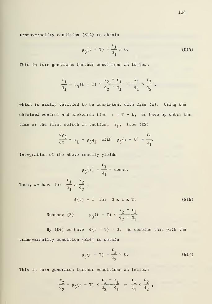
134

transversality condition (E14) to obtain

ri

p (t = T) = — > 0. (E15)q l

This in turn generates further conditions as follows

r r = r r r— = p_(t = T) > — k =» — > -*,

q l3 q

2" q

lq l q

2

which is easily verified to be consistent with Case (a) . Using the

obtained control and backwards time t = T - t, we have up until the

time of the first switch in tactics, x , from (E2)

dp3

rl— = r

x- p 3qi

with p3(x - 0) -—

.

Integration of the above readily yields

P-,(t) = — = const.ql

r r1 2

Thus, we have for — > —,

q l q2

<|>(t) = 1 for £ t £ T. (E16)

r - r

Subcase (2) p_(t = T) < — ~3 q

2- q

l

By (E4) we have <j>(t = T) =0. We combine this with the

transversality condition (E14) to obtain

r2

p (t = T) = — > 0. (E17)q2

This in turn generates further conditions as follows

r r - r r r-^ = p_(t = T) < -^ ± * -± < -±

,

q2

P3 q - q q q

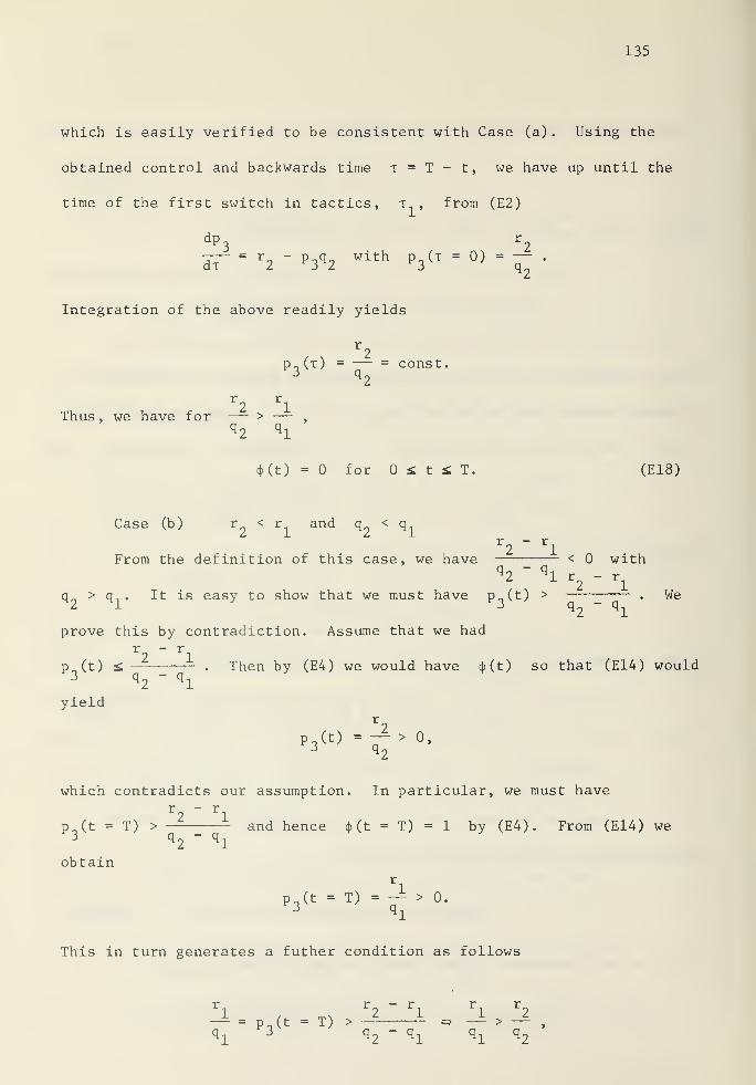
135

which is easily verified to be consistent with Case (a). Using the

obtained control and backwards time T = T - t, we have up until the

time of the first switch in tactics, i , from (E2)

dp3

r2— = r

2- p

3q2

with p3(x = 0) = — .

Integration of the above readily yields

p„ (x) = — = const.q2

r r2 1

Thus, we have for — > —,

q2

qx

(t) = for i t s: T. (E18)

Case (b) r < r and q < q

r — r2 1

From the definition of this case, we have < withq2

" ql r

2- r

q^ > q, . It is easy to show that we must have p n (t) > . We21 q 2~ q

l

prove this by contradiction. Assume that we hadr — r2 1

p„(t) £ . Then by (E4) we would have d>(t) so that (E14) would3 q

2" q

x

yield

P 3(«-^»0.

which contradicts our assumption. In particular, we must haver - r

p_(t = T) > — and hence <\> (t = T) = 1 by (E4). From (E14) we3 q

2" q

x

obtain

P3(t - T) - II > 0.

This in turn generates a futher condition as follows

ri

r2

" ri

ri

r2-^ = p.(t = T) > -^ i => -^ >

-f- ,

q l3 q 2

" q l ql

q2

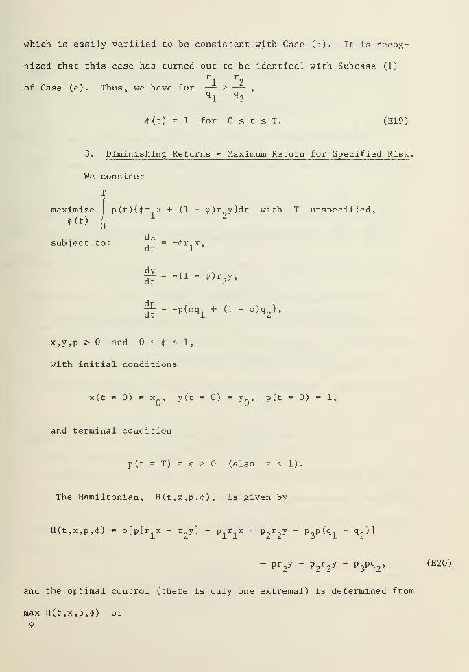
which is easily verified to be consistent with Case (b). It is recog-

nized that this case has turned out to be identical with Subcase (1)

ri

r2

of Case (a). Thus, we have for — > —,

nl H

2

<t>(t) = 1 for s. t £ T. (E19)

3. Diminishing Returns - Maximum Return for Specified Risk ,

We consider

T

maximize

00p(t){<j>r x + (1 - c£>)r y}dt with T unspecified,

subject to:dx

dt~= -* r

iX '

£--<l-*>V>d£ = _dt p{<f>q

1+ (1 - 4>)q

2h

x,y,p ^ and <_ <$> < 1,

with initial conditions

x(t = 0) = xQ

, y(t = 0) = yQ

,p(t = 0) = 1,

and terminal condition

p(t = T) = e > (also e < 1).

The Hamiltonian, H(t,x,p,<j>) , is given by

H(t,x,p,<{>) = <()[p{r1x - r

2y} - P-^x + P

2r2y " p

3P ^q l

" q2) "'

+ pr2y - P

2r2y - p^, (E20)

and the optimal control (there is only one extremal) is determined from

max H(t,x,p,<j>) or

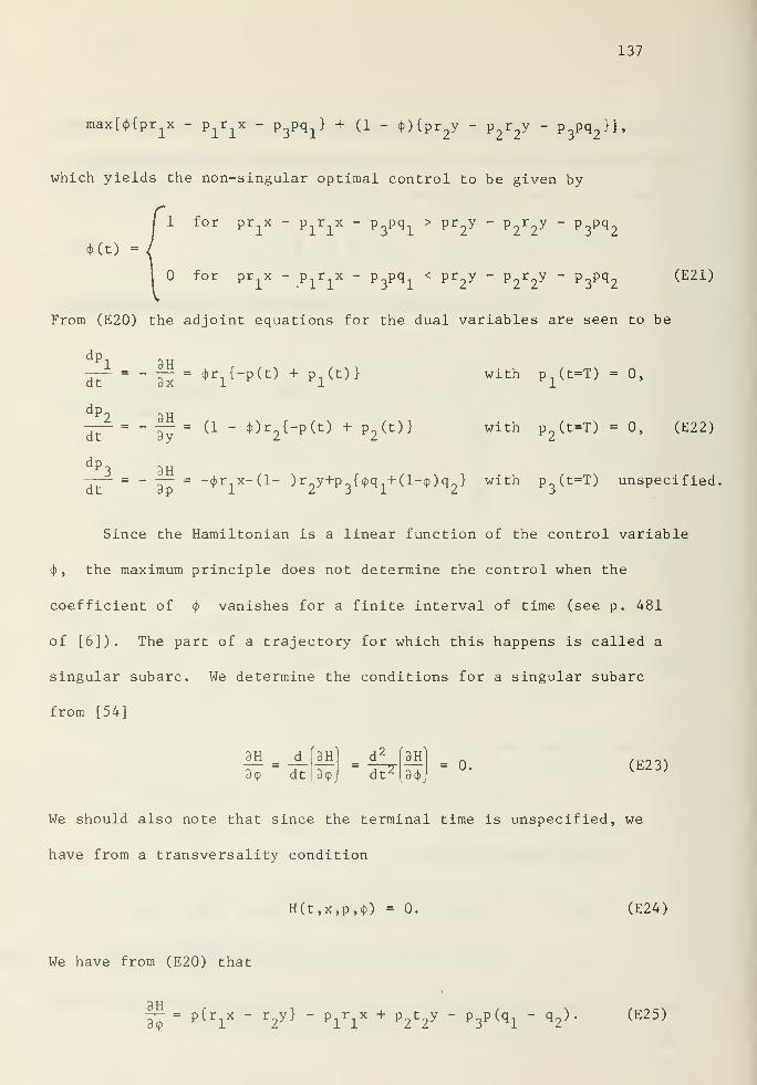
137

max[<t){pr1x - P-^x - P

3Pq

1) + (1 - <J>){pr

2y - P^y - P

3Pq

2^

which yields the non-singular optimal control to be given by

for prxx - P-^x - P

3Pq

1> pr

2y - P

2r2y -

p3pq

2

*(t) =

for pr1x - P

1r1x - P

3Pq

;L

< P^y - P2r2Y - P

3P C

12

(E21 )

From (E20) the adjoint equations for the dual variables are seen to be

dp,

dt

dp

dt

dp.

dt"

i--_!f-*r1{-p<t> + p 1

<t>>

£- -|5. (1 - 4,)r2{-p(t) + p

2(t)}

with p (t=T) = 0,

with p2(t=T) = 0, (E22)

3H— = -<f>r x-(l- )r y+p {<|>q +(l-<|>)q } with p (t=T) unspecified,

Since the Hamiltonian is a linear function of the control variable

<J), the maximum principle does not determine the control when the

coefficient of<J>

vanishes for a finite interval of time (see p, 481

of [6]). The part of a trajectory for which this happens is called a

singular subarc. We determine the conditions for a singular subarc

from [54]

_d_

dt

3H

84)

'2 <*Y?

dt' 3<J>_

= 0. (E23)

We should also note that since the terminal time is unspecified, we

have from a transversality condition

H(t,x,p,cf)) = 0. (E24)

We have from (E20) that

3 H— = p{r1x - r

2y} - P-^x + P^y - P

3p(q

1- q

2>. (E25)

138

A rather lengthy computation, which makes use of both the adjoint

equations (E22) and the state equations, yields

it*)= "P(q

2rix - q

ir2y) - (E26)

By (E23) and (E26) , we see that a condition for a singular subarc is

thatrxx r y

-±- = -*- (E27)q l q

2

The singular control is determined from requiring that it keep us on

the singular subarc. Thus, (E23) and (E26) yield (note that -rjj: £

and p + 0)

dx dy _~q2ri dT

+ q lr2 d?

= °

or using the state equations,

q2ri

rlX ~ q

ir2(1 " <t>)r

2y =

°

orr,x r y

Using the fact that we are on a singular subarc so that (E27) holds,

we obtain the singular control as

r2

* - . % _ • (E28)

1 2

A necessary condition for the singular subarc to yield a maximum

return is that [57]

J_ ,d 2

34>ldt z

[3<()

3H} £ 0. (E29)

139

From (E26) we have that

d 2

dt 23H

^(p{-q2r1x+q

1r2y})

dpf

,,

, dx dy=dt {

-q2riX+q

ir2y}+p{ - r

iq2 o7

+ r2ql dP'

or, using the state equations,

dt'

3H

3<J>

-p{(J)q1+(l-4>)q

2}(-q

2r1x+q

1r2y)+ pr^ r^x - pr^U - cfO^y.

and hence

9r

d 2

3<f> dr3HW } = p(-q

1+ q

2)(-q

2rlx + q-^y) + pO^^x + pCr^^y,

On the singular subarc we must have (E27), so that the above reduces to

3_(d 2

3d> dF73H

l3<t»J

} = p{(r1

)2q2x + (r

2)2

q;Ly} > 0, (E30)

and the necessary condition is satisfied.

It is convenient to define (where t is backwards time defined

by t = T - t)

A(x) = prxx - P-^x - P

3Pq1 >

and B(t) = pr2y - P

2r2y - P

3pq

2> (E31)

Then (E21) may be written as

*(t) =

1 for A(t) > B(x)

for A(t) < B(t), (E32)

140

with the singular control

Also

r + r1 2

for A(t) = B(t) (E33)

dA dA d ,,

dT= " dT

=oT c"Pri

x + pirix + P

3pq

l) '

and a laborious computation, which makes use of both the adjoint

equations (E22) and the state equations, yields

— = p(l - 4>)qiq 2

r2y

^ (E34)

Similarly

dBdT

= p * qiq2

r2y r

iX

I q 2

(E35)

We develop the solution by working backwards from the end of the

problem at t = T . We start by determining the boundary condition on

p~ at the end. There are two cases to be considered: either we are

on a singular subarc at t = T or we are not.

If we are on singular subarc, then by transversality condition

(E24) and condition of singular subarc = , we have

pr2y " P 2

r2y " P

3Pq

2=

° '

which yields by use of the boundary conditions on (E22)

r9y(t=T)

(E36)

We also note that on the singular subarc (E27) applies.

141

If we are not on singular subarc, then there are two further

subcases: either cj>(t = T) = 1 or <f>(t = T) = 0. If <j>(t = T) = 1,

then (E20) , the transversality condition (E24) , and the boundary condi-

tions on (E22) yield

r..x(t = T)

p ( t - T) - ^— . (E37)ql

Since (t = T) = 1, then by (E21) and fact that p (t = T) = p (t = T) =

we have

prlX " P

3Pq

l> pr

2y ~ p

3pq 2'

and hence

r x(t = T) r y(t = T)— > -. (E38)ql

q2

A similar development shows that for cf>(t = T) = 0, we must have

r x(t = T) r y(t = T)-^— < -*— . (E39)

q l q2

We now trace the optimal trajectories backwards from the end,

From the above, we have three cases to consider.r,x r y

Case (1) at t = T, —— > -=-~ql

q2

In this case by (E38) we have <|> (t = T) = 1. From (E21) and

boundary conditions we have

A(t = 0) > B(t = 0)

Then up until the time x of the first switch in tactics we have from

(E34) and (E35)

142

£-»and

and hence

dB

d7= Pq lq 2

r2y rx

{ q 9 ^

< o,

A(t) = A(x = 0) > B(t = 0) > B(t).

Thus , we have

<j>(t) =1 for £ t £ T. (E40)

Case (2) at t = T,

r]_x r

2y

q l q2

A similar argument shows that

<|>(t) =0 for £ t £ T. (E41)

Case (3) at t = T,

riX r

2y

q l q2

We see that this corresponds to when the system ends up on the

r2

singular subarc at t = T. In this case d> (t = T) = ;

, and wer + r '

continue (in backwards progression) to use the singular control

<J>(t) = r„/(r n + r_) (note that — = — = when this is used and2 12 dx di

that we had A(t = 0) = B(t = 0)) until x(t) = x or y(t) = y .

This yields three further subcases.

r„ x„ r„\r1 2^0

Subcase (3A)ql q 2

We use <j)(t) = r / (r + r ) from the beginning

rixo

r->yo

Subcase (3B) -^-^ > -=-=ql

q2

143

Define t. as t such that y(t-, > 0) = y . Then we use

4>(t) = 1 for si t £ t . This is consistent since A(t = T - t, )

B(x = T - t..). Then up until the time x of the next switch in tactics

we have from (E34) and (E35)

dAdT

= 0,

and

and hence

dB

dT= pq

iq2

r2y r

xx

I q 9 <hi< o,

A(t) = A(t = T - t ) = B(t = T - t ) > B(t)

From (E32) we see that

<|>(t) = 1 for T - t s£ T £ T, (E42)

Subcase (3C)

r x r v10 2*0<

Hl

H2

A similar argument as that for Subcase (3B) with the roles

of x and y interchanged readily shows that

(t) = for T - t £ t £ T. (E43)

Note that in the above developments we have implicitly made use of the

non-negativity of the state variables.

4. Diminishing Returns - Prescribed Duration Use .

We consider

maximize

CO '

pCtM^x + (l <j>)r9y}dt with T specified,

144

i . dxsubject to: — = -^r.x,

dt 1

j£ = -p{ (|,qi+ (1 - <},)q

2},

x,y,p ^ and £ <() £ 1,

with initial conditions

x(t = 0) = xQ

, y(t = 0) = yQ

, p(t = 0) = 1.

The development of the solution to this problem is similar to

that of maximizing return for a specified risk. We have considered the

latter problem in Section b3. above. Two main differences between these

problems are that (1) the boundary conditions on the dual variables at

t = T are slightly different and (2) for the present problem the total

time is specified so that the transversality condition H(t = T,x,p,<£) =

no longer is applicable. In view of the similarities, we shall frequently

summarize results from the previous problem which apply to this one.

The interested reader can, of course, refer to the previous problem for

full details.

The Hamiltonian, H(t ,x,p , <j>) , is given by

H(t,x,p,c)>) - <|>[p{r1x - r

2y} - P-^x + P

2r2y " P

3p(q

l" q2^

+ pr£y - P

2r2y - P

3pq

2- (E44)

The adjoint equations for the dual variables are the same as (E22) with

the exception that the boundary conditions at t = T are now

P]_(t = T) = 0, p2(t = T) = 0, p

3(t = T) = 0. (E45)

145

The non-singular control obtained by maximizing the Hamiltonian is given

by (where, as before, t is the backwards time defined by t = T - t)

(x) =

1 for A(x) > B(t)

for A(t) < B(t), (E46)

where

A(t) = prxx - P

1r1x - P

3Pq

1

B(x) = pr2y - P

2^2y - P

3pq

2. (E47)

As above, it may also be shown that

dA n ^— = p(l - 4»)qiq 2

r ]X r2y^

I el-

and

V rxx

aT =P * qlq2 lq2 q±j

It is convenient for a later development to define

(E48)

D(t) = A(t) - B(t), (E49)

so that (E46) becomes

4><t) =

1 for D(t) >

for D(t) < 0. (E50)

Using (E48) and (E49) we readily obtain

dD

dT= Pq

lq2

^x r2y

Iq- q

2J

(E51)

146

with

D(x = 0) = p(r1x - r

2y), (E52)

where we have made use of (E45) besides obvious definitions.

Since the Hamiltonian is a linear function of the control variable

<}> , the maximum principle does not determine the control when the

coefficient of 4> vanishes for a finite interval of time (see p. 481

of [6]). We recall that the part of an optimal trajectory for which

this happens is called a singular aubarc. As in the previous problem

on a singular subarc we have

r x r y-± j- ,

(E53)ql

q2

with the singular control to remain on it given by

r2

<f>=

; . (E54)

1 2

Again, it is readily verified that the necessary condition for the

singular subarc to yield a maximum return [57] is met.

Let us now examine the determination of the optimal control at

the end of the problem t = T or t = 0. Substituting the boundary

conditions (E45) into (E47) , we obtain

and

and hence (E46) becomes

A(t = 0) = prx,

B(t = 0) = pr2y, (E55)

(t - T) -

1 for r x(T) > r2y(T)

for r x(T) < r y(T). (E56)

147

In contrasting the optimal trajectories and tracing the optimal

course of the bomber utilization (backwards from the end of the prescribed

duration period of usage) it is convenient to consider the following.

We recall that the optimal control is determined by the sign of D(t)

(see (E50) , (E49), and (E47)). From (E53) a singular subarc must occurrxx r

2y

on the line L defined by — = — . We recall that at the end ofql

q2

the planning horizon x = 0, we have

D(x = 0) = p(t = T){rlX (t = T) - r2y(t = T)

}

Consider now the line L' defined by r x = r„y. This line will lie

above, on, or below the line L defined by

riX r

2Y

depending

on whether q is greater than, equal to, or less than q . This is

evident from considering the slopes of these two lines which pass through

the origin

dy_

dx

dy_

dxL'

and hence, for example,

dy_

dxL 1

dy_

^dx.for q

x> q

2.

The significance of the line L' and its relationship to the line L

is that

> below L'

D(t = 0)

< above L'

,

(E57)

148

and hence by (E50) we find that

1 below L1

for P(T) above L'

,

(E58)

where P(t = T) = (x(t = T),y(t = T)). We also note from (E51) that

> below L

dD(-c)

dx

< above L. (E59)

Thus, (E59) and (E59) give us three cases to consider

Case (a) q = q2

= q,

Case (b) q > q2

,

Case (c) q 1< q .

For Case (a): q.. = q~ = q, equation (E51) and initial condition

(E52) are

dD , .- = pq(rlX - r2y)

with

D(t - G) - pCr^x - r2y).

There are three cases to consider depending on the sign of D(t = 0).

Case (1) r1x(t = T) = r y(t = T)

We see that this corresponds to when the system ends up on ther2

singular subarc, i.e., D(x = 0) = 0. In this case <j>(t = T) =r + r '

1 2

and we continue (in backwards progression) to use the singular controlrxx r

2y

<$>(t) = r /(r. + r_) to remain on = (note that this makes212 ql q

2

149

— = and that we had D(t = 0) = 0) until x(t) = x^ or y(t) - y„,dx *

This yields three further subcases.

Subcase (1A) riXQ

< r2Y

Define t, as t such that x(t > 0) = x . Then we use

t()(t) = 1 for £ t £ t. . This is consistent by the following. At

t = T - t , we have D(t = T - t ) = and up until the time x of

the next switch in tactics we have

dD , , NX— = pqCr^ - r2y(x)) < 0,

for T - t £ x £ T and hence

= D(x = T - t ) > D(x).

From (E50) we see that

<|)(t) =0 for T - t £. T £ T. (E61)

Subcase (IB) r x > r y

A similar argument as that for Subcase (1A) with the roles

of x and y interchanged readily shows that

4>(x) = 1 for T - t £ x £ T. (E62)

Subcase (1C) r x = r y

We use (})(t) = r / (r + r ) from the beginning.

Case (2) r x(t = T) < r y(t = T)

In this case we have D(x = 0) = p{r x(t = T) - r y(t = T)} < 0,

and by (E50) at the end of the planning horizon we have <j>(i = 0) =

so that y(x = 0) < y(x) for x > 0. Thus we have until the time x..

of the first switch in tactics

150

|^ = pq{r1x(t = T) - r

2y(x)} < 0,

for £ t £ x and hence

> D(x = 0) > D(t).

From (E50) we see that

(j>(t) =0 for £ t ^ T. (E63)

Case(3) r^t = T) > r2y(t = T)

A similar argument as that for Case (2) with the roles of x and

y interchanged readily shows that

4>(t) = 1 f°r ^ t ^ T. (E64)

We now consider Case (b): q > q . There are two cases to be

considered.

Case (1) never on singular subarc for finite interval of time

Again there are two subcases to consider, depending on whether

the system winds up above or below L.

r x(t = T) r y(t = T)

Subcase (la) >

ql

q2

The definitions of Case (b) and Subcase (la) imply

r.x(t - T) q

r2y(t = T)

> V2> ly

so that we have

rxx(T = 0) > r

2y(x = 0)

151

Thus by (E52) D(t « 0) > and hence by (E50) <j>(t T) - 1. We

consider now the x-time interval up until the time t. of the first

switch in tactics. Use of $(t) = 1 for xe[0,x..] results in x(t) >

x(x = 0) for x > 0. Recalling that

dD

dT= pq

iq2

r x( T ) r y( T = 0)

ql

q2

for xe[0,x..] and the definition of this case, we easily see that

dD A A U-r~~ > and hencedx

< D(t = 0) < D(t).

From (E50) we see that

4»(t) = 1 for <; t £ T. (E65)

rxx(t = T) r y(t = T)

Subcase (lb) <

q lq2

Again there are two further subcases to consider, depending

on whether the system winds up above or below L'

.

r x(t = T) r y(t - T)

Subcase (lbl) < and r, x(t = T) <

q-Lq2

"I

r2y(t = T)

In this case we wind up above L 1. Since D(t = 0) is given

by (E52), we have D(t = 0) < and hence by (E50) <j> (t = 0) = 0. Since

we are initially above L and remain so by use of <J>(t) = 0, we have

by (E59) -p- < for all te[0,T] and hence D(t) < for all r.dx

Thus we have

4>(t) =0 for S t S T. (E66)

152

r x(t = T) r y(t = T)

Subcase (lbll) and r,x(t = T)qx q

2-1

r2y(t = T)

In this case we wind up below L1 at the end. Since

D(t = 0) is given by (E52), we have D(t 0) > and hence by (E50)

<j> (t = 0) = 1. We work backwards from the end. Since we are above L,

— < while we remain above L. Thus D(t) decreases for x> whileax

we remain above L. There are two further subcases depending on whether

D(t) decreases to zero before the line L is encountered. Let x..

be such that D(x ) =0. If L has not yet been reached at t , then

D(t) for x > x1

is negative and 4>(t) = until the beginning of

battle. It is also possible that the system just reaches L the instant

that D(x ) = 0. In this case (assuming we don't remain on singular subarc)

D(t) > for t > T, , since we pass below L and then — > 0.1 r dx

Case (2) on singular subarc for finite interval of time

r^xCt = T) r y(t = T)

This can happen only when < and r.x(t = T) >

ql

q2

l

r~y(t = T). As usual, we work backwards from the end of the planning

horizon. We use <J>(t) = 1 for £ t £ x , and at x = x we mustr x(t ) r

2y ^ T

i^have = . We use the singular control 4(x) = r„/(r 1 + r„)

q x q2

2 12for t

1aE x £ x

?. There are three further subcases

(1) x(t2

) = xQ

, y(x2

) < yQ

,

(2) x(x2

) < xQ

, y(x2

) = y ,

(3) x(t2

) = xQ

, y(x2

) = y Q.

We omit the trivial discussion of these cases.

153

Thus, to summarize, we see that there are six possible cases for

the history of the strategic worth of the two target areas in the use

of the bomber for a prescribed length of time:

(1) started below L and never reached L,

(2) always above L'

,

(3) started above L' and end up above L but below L'

without ever reaching L,

(4) end up above L but started below L and did not remainon L for finite interval of time,

(5) started above (or on) L and were on L for finiteinterval of time

,

(6) started below L and were on L for finite interval of

time.

Case (c) : q < q is similar to Case (b).

c. Summary of Solutions .

In this section we summarize the solutions developed in the

previous section for the four versions of the continuous stochastic

gold-mining problem. We shall summarize the cases of non-diminishing

and diminishing returns separately.

The solution for the case of non-diminishing returns is shown in

Table EI. We note that for both cases considered the optimal policy

is independent of the current strategic values of the two target areas,

i.e., the state variables. For the case of maximizing the return for

a specified risk, the optimal policy is independent of the risk (cumula-

tive probability of bomber being shot down) and depends only on the

r

.

ratios of — which we may interpret as the expected gain per unitqi

time divided by the expected loss per unit time.

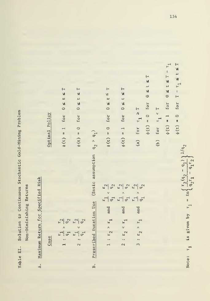
154

6CUHX>OUCL,

bO

•Hc•Hs

I

id-HoOo•H4-J

CO

co

J=oo4-)

CO

co

o

c•H4-1

coCJ

O4J

do•H

oCO

wcu

a

CO

C>-i

3u0)

Pi

Ma•HXiCO

•Ha•He•HQ

I

CoS3

CO

•HPd

CU

Ocu

en

o

au

•UCU

§6•HXcd

S

5•HrHoPm

CO

E•H4J

ao

cu

CO

vi

4-)

VI

o

HVI

4-1

VI

o

J-l

o<4-l

oII

CM CM CM CMs-i

Icr u

Ia*

A V

Hi H Hi Hu

|cr U

I o"

rH CN

cr

A

CMcr

CO

CO

PQ

«

HVI

4-1

VI

o

oII

/—

-

4-J

^—

'

-e-

HVI

4J

VI

o

uo

14-1

4-1

-e-

rHH

1

HVI

HVI

1

HVI

4J

4-1 4-1 y->

VI VI I

o o H

Huo4-1 H

5-1

O14-1

V-i

o14-1

Ai V

H 4-1 H 4-J

<W -e- «4H -©-

CM CM CM CM CM CMu cr s-i cr 5-4 cr

cr

TJccO

13CJCO

eCO

rHu

HJ-i

r

A V A

CM CO

CMcr

cr

i

CMcr

CM

CMUrH

cr

i

uCM

X>

ccu

>•H&0

CO

•H

o

155

For the case of prescribed duration use with non-diminishing

returns, we consider the case of q_ > q1

with the other case being

similar with the roles of x and y interchanged. The condition

q ?> q means that there is a larger risk per unit time of the bomber

being lost over the second target area. Consider the planning horizon

of length T. During the closing stages of length t, of this bombing

campaign, we send the bomber to the target area of greater return per

unit time regardless of the risk. The length of this interval, x ,

is, of course, dependent on the risks involved and will be shorter as

the chances of the bomber being shot down over target area two become

greater. During the initial stages of the bombing campaing, i.e., for

£ t £ T - t , we allocate the bomber giving consideration to the

risks, and the solution is identical to the previous case.

When there are diminishing returns, the solution is seen to

depend on the strategic values of the target areas. Consequently, we

have chosen to plot the optimal policies as a function of the state

variables.

The case of maximizing return for a specified risk with diminish-

ing returns is shown in Figure El. It is seen that the line L definedr-jX r

2y

by — = plays a central role in the solution. We may interpretq l

q2 r

xx

a quotient like —— as representing the expected return per unit timeql

divided by the expected loss per unit time for operating in the target

area. Another way to do this is return per unit cost per unit time.

The optimal policy is to send the bomber to the target area which

maximizes the return per unit risk (cost). In this respect this solu-

tion is identical to that of non-diminishing returns except now, of course,

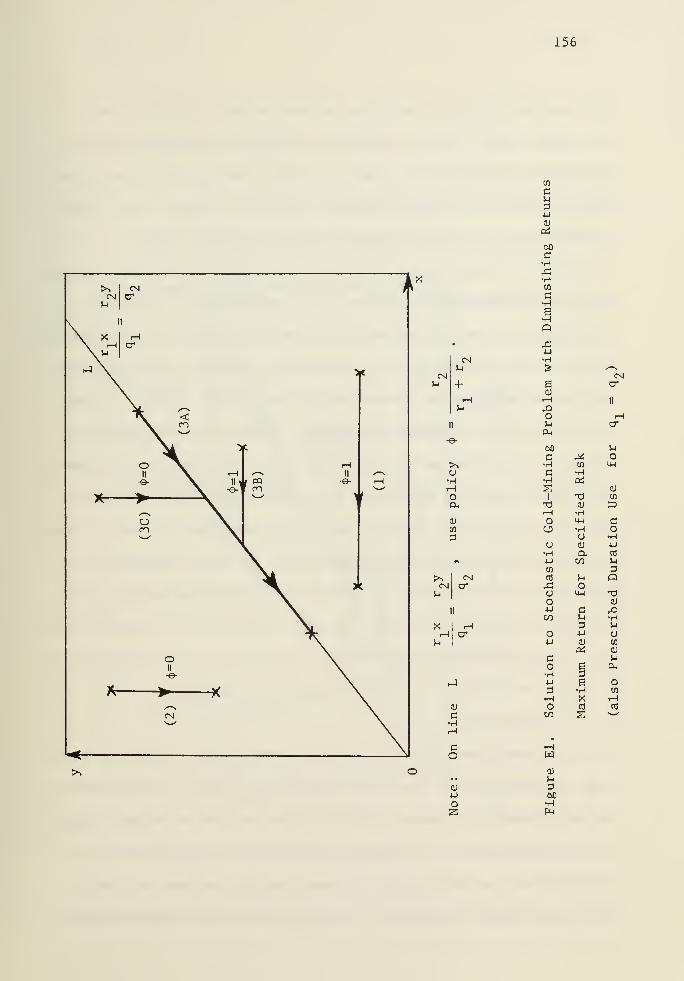
156

co

Cu3•u

a)

pcj

aoC•H43Hen

C•Hg•Ho

• 42u

(N •H1-1 S /—N

CN CMU + 6

a)

cr

rH rH ll

U 43O rH

II U cr

-e-&o Mc r« O

>^ •H to 4-1

a C •HH •H cdH s a)

O 1 -a CO

a T3 0) ^rH •H

0) O 4H C0) u •rH o3 U •H

O 0) 4J

•H a Cfl

n 4-1 co uCO 3

>^ CN cd s-i QCN cr 43 o

r4 o 4H -Oo OJ

II •U a 43co u •H

X rH a S-J

rH cr o 4J aM 4-1 OJ CO

cd a)

C Mo 1 P-i

•H dhJ 4J e O

3 •iH CO

^H X rH<u O fO Cfl

d CO S *—

'

HrH

C rHO W

CD• • uQJ d

.u Mo

fu

157

the expected return per unit time depends on the strategic value of

the target area. The paths labelled on Figure El correspond to the

nomenclature of Section b3. above. We note that this solution is the

same as that for prescribed duration use when q = q 9, i.e., there

is equal risk of losing the bomber in the two target areas.

For the case of prescribed duration use with diminishing returns

there are three cases to consider. The solution for Case (a) : q = q

is the same as that for maximizing return for specified risk as discussed

above. The case when q. > q„ is shown in Figure E2. The paths are

denoted according to our terminology of Section b4. Again, consider

the total time of the bombing campaign. During the early stages we

allocate giving consideration to risks, but during the closing stages,

the bomber is sent to the target area yielding the greater return per

unit time (as measured by r x and r y) regardless of risk. Although

we have not made an explicit determination, it seems reasonable to

conjecture by analogy with the case of non-diminishing returns that

the greater the risk at target area one, the shorter this interval will

be. During the previous period, i.e., £ t £ T - t.. , the bomber is

allocated on the basis of return per unit cost as before.

d. Discussion .

We have already noted for the non-diminishing returns the alloca-

tion is independent of the state variables and effort is concentrated

on one alternative, whereas for diminishing returns the values of the

state variables must be considered and effort may be split over the

alternatives. We shall point out some similarities with the combat

allocation models of Appendix C and then attempt some generalizations.

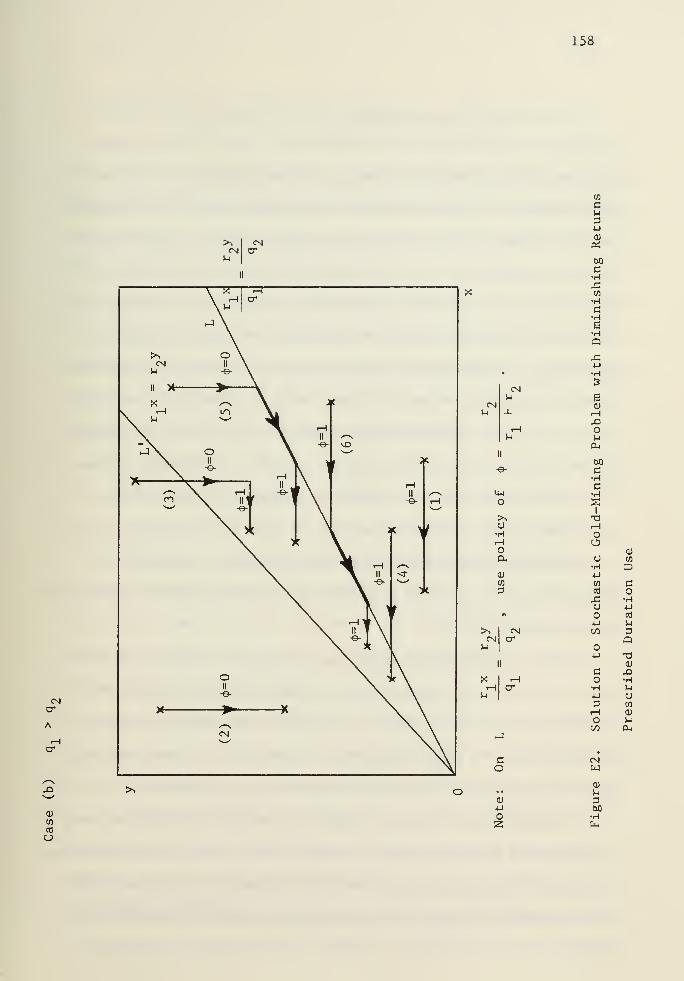
158

>* CMCM crU

cr

en

c>-l

34J

OJ

Pi

ooc•Hx;en

•H3•Hs•HQ

CD

en

CJ

M 6CN 03U 4- H

XirH OU U

fX4

II

60-e- 3H

314-1 «H

s1

>^1

n3rH

•H OrH OO CD

a, a cn

•H 3a> •uen en 33 erj O

XI •H4-1

fl crj

4-1 U>^ CN w 3CM cr QM

4J -3II 0)

3 XiX rH •HH cr •H MJ-i 4J O

3 en

rH a)

O MCO P-,

hJ

3 CNO w

CD

CD 31j 60o

fa

159

We should note the similarity of the structure of the optimal

allocation policies with that in selection of target type in combat

described by Lanchester-type equations. There appears to be an under-

lying structure for allocation with diminishing returns and allocation

with non-diminishing returns. Let us recall that for a square law

attrition process, the attrition (return) per unit time per unit of

weapon system is a constant; whereas for a linear law attrition process,

the attrition (return) per unit time per unit of weapon system is

proportional to the number of targets remaining (diminishing returns).

This observation has prompted our conclusion in Appendix C that fire

is concentrated on a single target type only when the fire is "aimed"

and the target acquisition rate is not subject to diminishing returns.

We also note that the termination conditions of the scenario

(prescribed time or use until reach given level of risk) has an effect

upon the optimal allocation policy. We have noted in Appendix C a

similar result for tactical allocation in combat described by Lanchester-

type equations.

When we compare the results from the Lanchester attrition models

to the stochastic gold-mining problems, the allocation appears to be

different when one is not subject to a cost (loss) from the alternative

not being used. It seems appropriate to consider in future work this

type of attrition model to see what insight may be provided.

We seem to have uncovered a general principle (although we most

likely are not the first) that allocation in the face of non-diminishing

returns and diminishing returns are two fundamentally different cases.

With diminishing returns, we must constantly observe the state of our

system.

160

APPENDIX F. A New Dynamic Kill Potential.

In this appendix we propose a dynamic measure of combat capability

by means of the adjoint system of differential equations for Lanchester-

type equations of combat. The current results are of a preliminary

nature and may be revised in the future.

What is a quantitative measure of effectiveness for a combat unit

or weapon system? In many circumstances it appears to be the rate of

destruction of the enemy. A more sophisticated approach is to consider

the rate of destruction of enemy capability as measured by the rate of

destruction of his kill rate against the friendlies.

We have devised a simple way to determine a dynamic kill potential

which is the rate of destruction of enemy kill rate giving full consid-

eration to the future course of combat. Consider a weapon system of

constant kill rate capability employed in combat against an enemy.

The loss of such a weapon is weighted more heavily in the early stages

than in later ones. This is because of the "multiplying effect" of the

dynamics of combat, i.e., loss of a weapon is also loss of future

killing capability of the weapon.

Such a concept has application to force structuring and weapon

system analysis. In such work, frequently a large number of alternatives

have to be screened. It is infeasible to assess the effectiveness for

all the alternate force/weapons mixes by a computer simulation of a

standardized scenario. The concept of firepower scores and weapon

firepower potential have been developed to screen out unattractive

alternatives in preliminary analyses. We have extended these concepts

to consider the true dynamics of combat. Originally we were motivated

161

by the interpretation of the adjoint system of differential equations

in optimal control theory.

In this appendix we state the problem, give some additional back-

ground, and then propose our solution. We then comment on other

applications of these ideas before presenting a brief justification of

our concept. Finally, we point out the deep relationship of this seem-

ingly simple notion to linear analysis.

This is our initial effort on this problem from a purely mathe-

matical point of view. For the future, we would propose to compare

firepower potentials computed by current methods and by our new method

and also to improve and expand the exposition. We are currently super-

vising a student thesis on this topic from a more applied standpoint

("Weapon Firepower Potential" by Major James B. Taylor, USA).

a. Statement of the problem .

To devise a quantitative measure of the combat capability of a

unit/weapon system giving consideration to the dyanmics of combat.

b

.

Some Background .

We could consider a "static" kill potential, the rate of destruc-

tion of the enemy kill rate against the friendlies not considering the

future course of battle. The concept of firepower scores has evolved

into the notion of weapon firepower potential. The latter considers

attrition rates as we have indicated but in a "static" fashion. In

practice, analysts use operational ammunition consumption rates and

operational kill/hit probabilities to estimate attrition rates. Infor-

mation systems have been designed to make available such information

on various systems in numerous circumstances. A high degree of sophistication

162

is not warranted for estimation of kill rates because of the uncertainty

in the data.

The current approach to weapon firepower potential does attempt

to consider combat dynamics in the following fashion: kill rates are

weighted more heavily at the longer ranges. This recognizes the advan-

tage of destroying the enemy at longer ranges before he becomes more

effective at killing friendlies at the closer ranges.

What we need is a measure which considers the dynamics of combat:

losses early in battle effect the outcome by evolving into more enemy

survivors and less friendlies. In the next section we show how to use the

concepts of operational definition and adjoint system of differential

equations to account for combat dynamics.

c. The Proposed Solution .

We employ the concept of an operational definition (see Chapter

5 in [1]) by defining a dynamic firepower potential of a unit/weapon

system under precise circumstances. Numerical measures can only be

meaningfully compared under the applicable circumstances.

We consider a standardized scenario of combat between an X-force

and a Y-force in a battle lasting a prescribed time T. For illustra-

tive purposes we consider the case of constant attrition rates. Our

approach explained in Appendix D allows many variable attrition rate

cases to be solved in closed form. This approach applies equally well

to the adjoint system of differential equations considered here.

We consider the rate of return of a unit/weapon system (in terms

of destruction of enemy kill rate) as measured by the product of a

measure of enemy kill-rate worth and the enemy attrition rate by the

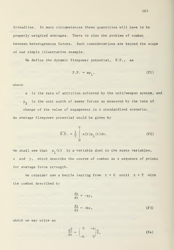
163

friendlies . In many circumstances these quantities will have to be

properly weighted averages. There is also the problem of combat

between heterogeneous forces. Such considerations are beyond the scope

of our simple illustrative example.

We define the dynamic firepower potential, F.P., as

F.P. = apr (Fl)

where

a is the rate of attrition achieved by the unit/weapon system, and

p is the unit worth of enemy forces as measured by the rate of

change of the value of engagement in a standardized scenario.

An average firepower potential would be given by

F.P. -

T

1a(t) Pl (t)dt. (F2)

We shall see that p (t) is a variable dual to the state variables,

x and y, which describe the course of combat as a sequence of points

for average force strength.

We consider now a battle lasting from t = until t = T with

the combat described by

dx

d7= ~ay '

^ = -bx, (F3)

which we may write as

dX

dt

-a>

X, (F4)

-b J

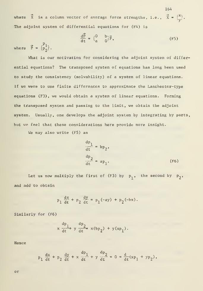
164

where X is a column vector of average force strengths, i.e., X =( ).

The adjoint system of differential equations for (F4) is

dt " U o^p

' (F5)

where P = [p„J .

What is our motivation for considering the adjoint system of differ-

ential equations? The transposed system of equations has long been used

to study the consistency (solvability) of a system of linear equations.

If we were to use finite differences to approximate the Lanchester-type

equations (F3) , we would obtain a system of linear equations. Forming

the transposed system and passing to the limit, we obtain the adjoint

system. Usually, one develops the adjoint system by integrating by parts,

but we feel that these considerations here provide more insight.

We may also write (F5) as

dPl„

dt K2

dp2' = aPl . (F6)

dtapr

Let us now multiply the first of (F3) by p , the second by p~,

and add to obtain

pi dT

+ p2 dt

= pi(_ay) + P

2(-bx) '

Similarly for (F6)

dP]_ dP2

x dT^ y dT^ x(bp2

} + y(api

} -

Hence

dx dy_dp

ldp

2 n d .

,PldT +P2di +X

dt-+y dr =C) =

dT(xp

l+ yP

2} '

or

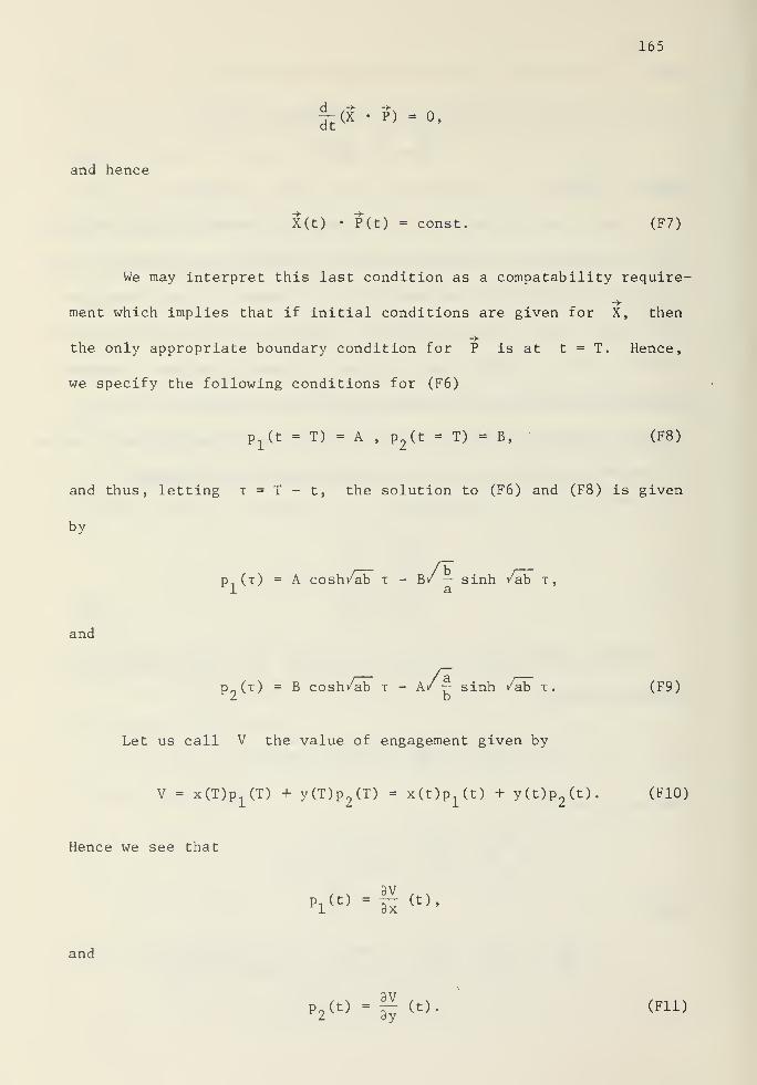
165

fj* -h-o,

and hence

X(t) • P(t) = const. (F7)

We may interpret this last condition as a compatability require-

->

ment which implies that if initial conditions are given for X, then

the only appropriate boundary condition for P is at t = T. Hence,

we specify the following conditions for (F6)

p±(t = T) = A , p

2(t = T) = B, (F8)

and thus, letting x = T - t, the solution to (F6) and (F8) is given

by

p n(t) = A cosh/ab t - Bv — sinh /ab x,

and

p.(x) = B cosh/ab x - A/ J sinh /ab x. (F9)L b

Let us call V the value of engagement given by

V = x(T) Pl (T) + y(T)p2(T) = x(t) Pl (t) + y(t)p

2(t). (F10)

Hence we see that

Pl (t) =^ (t),

and

p 9(t) = |^ (t). (Fll)

2 3y

166

We call p ,p„ dual variables, and they determine the combat's tra-

jectory in terms of line coordinates, whereas the state variables, x

and y, determine it in terms of point coordinates.

We have noted in dynamic tactical allocation models that if

surviving forces at t = T are assigned a worth proportional to their

kill rate, then target selection depends on the product of kill rates

(target and firer) . This has influenced our definition of dynamic kill

potential.

d. Some Comments .

The above is the same approach used by G. Bliss in developing

range tables for correcting artillery fire due to abnormal air densities,

weights of projectiles, winds, etc., shortly after World War I [17], [67].

We may think of the p's (dual variables) as the line coordinates of

the trajectory (path) of the battle represented by (F3), i.e., x = x(t)

and y = y(t) (the solution to (F3)) defines a curve in the x,y space.

The duality of Euclidean geometry (after adding the ideal point at infinity)

states that we may equally well represent a curve as either a sequence

of points (point coordinates) or as an envelope of tangents (line coordi-

nates). When points are transformed by a linear transformation, the

line coordinates are transformed by the transposed (or dual) matrix of

this transformation. Let us note that we may consider a linear differ-

ential equation to be the limit of linear equations.

e. Justification .

-> ->

We may use the condition X • P = const. to develop justification

for calling p the rate of change of the value of the engagement with

9Vrespect to X forces, -—

. Consider a battle lasting a specified8x

167

length of time T. Hence, we have

x(t)p1(t) + y(t)p

2(t) = x(T) Pl (T) + y(T)p

2(T). (F12)

If at time t the X commander had Ax(t) less troops, then this

would cause him to have less surviving troops at the end of battle

and the enemy (Y) to have more. In fact, the p's tell us how much

as we see below

(x(t) - Ax(t)) Pl (t) + y(t)p2(t) = (x(T) - Ax(T)) Pl (T) + (y(T) + Ay(T))p

2(T). (F13)

Combining (F12) and (F13) , we obtain

Ax(t)P;L

(t) = Ax(T)P;L

(T) - Ay(T)p2(T).

Letting p1(T) = 1 and p 9

(T) = -1, we see why I have referred to the

p's as the value of forces

Ax(t)p1(t) = Ax(T) + Ay(T). (F14)

From the above, we see that the variable p.. (t) shows what the effect

of the loss of one X soldier at time t would have on the outcome

of battle. Expressing the value of engagement, V, in terms of survivors,

we see that

Pl (t) -|* (t ) and p2(t) -|X (t).

Bliss's idea for the development of air density corrections for

the artillery range tables was similar.

168

f . Relation to Other Mathematics .

The underlying mathematical structure considered here (duality)

manifests itself in many of the modern operations research optimization

tools. Let us recall that we showed

. dX .* . dP T-+for — = AX and — = -A P

t

we must have

X • P = const. (F15)

The finite dimensional analogue of this relationship is

for Ax = b and A y = c

we must have

-*--*•-»>y • b = c • x. (Flo)

When extended to non-negative variables, this is

-* -> T-+ -»

for Ax = b and A y ^ c,

x ;>

we must have

y • b :> c • x. (F17)

The latter relationship may be used to develop many results in the

theory of linear programming. For example, an immediate consequence

is that for x that maximizes c • x subject to Ax = b and x ^ 0,

a sufficient condition is given by

T -ITA (B ) c^ - c £

D

169

-> -> ->

where B is non-singular matrix such that Bx = b and x is vectord B

of non-zero components of the solution. The above condition is

expressed in the linear programming literature as Z. - c. ^ 0.

To further indicate the fundamental nature of these concepts, we

note that a further generalization of (F15) is

for Lu(x) = f(x) and L v(x) = g(x),

we must have

(v(x)Lu(x) - u(x)L v(x)}dx = boundary terms, (F18)

where L is a linear differential operator and L is its adjoint.

This is known as Green's identity (p. 183 [62]) and has many important

applications to ordinary and partial differential equations. From it

one obtains the Green's functions for constructing solutions.

170

APPENDIX G. Applications to Deterministic Inventory Theory

In this section we consider the optimization of continuous review

deterministic inventory models by the Pontryagin Maximum Principle.

Several previously published results are extended. For linear produc-

tion rate costs, we show that when demand is known with certainty and

stock may be reordered at any point (continuously) in time, the optimal

inventory policy is to only order as needed and only do this after the

initial inventory has been depleted. The same type of policy is true

when there are budgetary constraints with the constraint being ignored

until the budget has been expended. We also have developed an alter-

nate method of analysis to that developed by Arrow and Karlin [3] for

the case of convex production rate costs. Our results on this latter

topic are not fully documented at this time.

Our reasons for considering inventory problems are twofold:

(1) such problems are a major aspect of defense planning and (2) our

previous research has considered operations research models with a simi-

lar mathematical structure. Our past research has uncovered several

facets of formulating and solving such dynamic models. For example,

by application of the theory of singular control [53], [54], [57], we

have shown that when the production cost rate function is linear, the

optimal inventory policy is insensitive to the nature of the shortage

(or penalty) cost function (as long as this is not pathological).

Our organization of this section is as follows: we review the

general deterministic inventory model and the shortcomings of the

classical calculus of variations methods for such a model before we

171

consider our sequence of- models. Then, we discuss the insight that we

have gained into optimal inventory policies. We begin by surveying

some previous work in the field of deterministic inventory theory.

An excellent introduction to elementary inventory theory and in-

ventory theory in general prior to 1957 is to be found in [26]. Dy-

namic models were not considered prior to 1951. A more advanced in-

troduction to inventory theory is by Arrow, Karlin, and Scarf [4],

who summarize work through 1958 and give an extensive bibliography.

Variational methods were applied to a deterministic inventory process by Arrow

and Karlin [3] in this work. An excellent survey of modelling tech-

niques and results has been written by Karlin [56] . Adiri and Ben-

Israel [2] attempted to extend the work of Arrow and Karlin by use

of the Pontryagin maximum principle. A comprehensive bibliography of

applications of optimal control theory to operations research problems

has been published by Tracz [77]. Considering this last reference, it

appears as though the above work and references cited therein represents

most of the published results on dynamic, deterministic inventory models.

Recently McMasters [63] has studied the Arrow and Karlin problem. How-

ever, we obtain here different results than McMasters has. Our results

are more in consonance with those of Arrow and Karlin [3].

a. The General Model .

We consider a deterministic inventory process subject to continu-

ous review. Karlin has an excellent discussion and classification of

inventory .models and our present discussion has been based on his [56].

We consider that all processes occur continuously in time. We shall

see that this leads to a problem in the calculus of variations. How-

ever, two factors that are commonly present in applications preclude

172

the direct application of the classical calculus of variations results

(1) non-negativity of variables and (2) inequality constraints.

Karlin [56] identifies four main factors in the inventory process:

(1) cost factors,

(2) nature of demand for inventory,

(3) nature of supply for inventory,

(4) mechanism of inventory process.

We assume a single item inventory. We consider a production cost,

c(u(t)) , per unit time which only depends upon the rate of production

u(t). We also consider storage or holding cost, h(l(t)) , which de-

pend upon the inventory level I(t). Orginally, h(I(t)) is only de-

fined for I(t) 2: , but we may extend this to I(t) < by con-

sidering shortage or penalty costs for not meeting inventory demand.

We omit considerations of the "time value of money" (discount rate).

The nature of the inventory demand is assumed to be perfectly

known and is given by r(t) , which is the demand rate. We consider

a deterministic supply without setup costs. The production rate is

denoted by u(t) . We consider an inventory process without lags and

continuous in time. Our decision criterion is the minimization of

total cost. The basic type of model we consider is the minimization

of a cost functional.

J[u] =(1

[c(u(t)) + h(I(t))]dt , T specified,

with the inventory being given by

173

Kt) = 1(0) +1

[u(t) - r(t)]dt.

The production rate is, of course, restricted to non-negative, i.e.,

u(t) ;> .

b. Shortcomings of the Classical Calculus of Variations .

We have already noted two model factors that prevent direct appli-

cation of classical calculus of variations results: (1) non-negative

variables and (2) inequality constraints. Our own research, however,

indicates that these difficulties may overcome by the formulation of

an equivalent problem. A similar approach may be used to develope many

non-linear programming results by the calculus [59] . For example, when

there are non-negative variables in our orginal problem, we may formu-

2late an equivalent problem by replacing x by u .We solve this

equivalent problem for u and then recover our orginal variable x.

Inequality constraints are easily converted to equality constraints by

the addition of non-negative slack variables.

c

.

Comments on Previous Work .

Our general comments are than when variational methods were at-

tempted before the advent of the Pontryagin maximum principle, little

more than a first variation approach leading to an Euler-Lagrange

equation was employed. We should note that the Pontryagin maximum

principle involves both the Euler-Lagrange equations and the Weierstrass

condition for the Weierstrass excess function. It is not surprising

that use of but one calculus of variations' tool from among many (there

are four well-known necessary conditions, i.e., Euler equation, Weierstrass

Legendre (second order) , and Jacobi conditions) has not been able to solve

all problems.

F. Morin [64] appears to be one of the first economists to formu-

174

late and attempt to solve a deterministic inventory model with con-

tinuous time. No backlogging of orders was allowed (no stockouts).

It should be noted that Morin tried to apply some theory developed

by Bolza (see [18] pp. 41-43) for extremal curves on the boundary of

the state space.

Arrow and Karlin [3] have solved Morin' s problem. Whereas Morin

tried to apply Bolza' s results directly to his problem, Arrow and

Karlin develop the solution to this specific problem by variational

methods. Anyone doubting the complexities of applying variational

methods to problems with non-negative variables and inequalities

should consult this work. In our notation the Arrow-Karlin problem

was

minu(t)

T

[c(u(t)) + h(I(t))]dt with T specified,

subject to: dl = u(t) _ r(t) ?

dt

and u(t) ^0 , I(t) :>0

with boundary conditions

I(t = 0) = 1(0) and I(t = T) = . (Gl)

Arrow and Karlin [3] solve the above model for linear holding rate costs

and general convex production rate costs. Their general solution algorithm

is applied to linear production rate costs and several other examples,

including quadratic production costs. The theoretical foundations of

Arrow and Karlin 's analysis are not immediately evident from the con-

175

tent of their paper which merely summarizes the results. The central

point is that one-sided variations are required when the inventory is

at a zero level. Arrow and Karlin apparently developed an extension

of the usual variational development for problems where convexity prop-

erties can be assumed. Their approach, however, does not seem to be

documented in any of the mathematical literature known to this author.

Adiri and Ben-Israel [2] applied to the Pontryagin maximum princi-

ple to Arrow and Karlin' s problem besides the classical optimal lot

size problem. However, because the boundary condition I(t = T) = ,

the value of the dual variable p(t) = (3 J* /9l) (t) is free at t = T

Since they never determine the value of the dual variable at t = T ,

i.e., p(t = T) , they never do solve this problem. In fact, their

conclusion as to the solution for linear production costs is unsupport-

ed by their analysis (the conclusion that the partial derivative of

the Hamiltonian with respect to the control variable is always nega-

tive is unsupported)

.

We re-examine the solution to the Arrow-Karlin problem given by

(Gl) above. The constraint; on the state variable I(t) ^0 implies

that we must have dl/dt ^ when I(t) = . Hence, we have

/ :> for I(t) >

u(t) <

L ;> r(t) for I(t) = . (G2)

We must further check to see if the state variable constraint has an

effect on the adjoint equation (see [24] p. 117), but we see that it

does not since (3/81) {dl/dt} = . The Hamiltonian is given by

176

H(t,I,p,u) = c(u(t)) + h(I(t)) + p(t){u(t) - r(t)},

so that the extremal control is given by

min {c(u(t)) + p(t)u(t)}. (G3)

u(t)

We note that p(t) > implies that the minimum of (G3) is given by

the minimum u(t) given by (G2) . The adjoint equation for the dual

variable p(t) = (3J /3I)(t) (see [12] for this interpretation) is

given by

dp_ . 3H _ dh

dt " 91""

dl

We introduce the backwards time x = T - t so that dp/dx = dh/dl and

hence

P(t) = ^ dx + p(x=0) .

dI

Because of the constraint I(t) ^ for all time, it is necessary to

consider two separate cases at x = 0. When I(t=T) > 0, then

p(x=0) = 0. This generates a further condition on l(t=0) so that

the end state I(t=T) > may be reached. When I(t=T) =0, it may

be shown that p(x=0) must be <0. The precise value of p(x=0) is

determined by further simultaneous conditions.

McMasters [63] also considers the above models. Unlike Arrow and

Karlin [3] who assumed that I(t=T) =0, he makes no assumption about

the inventory level at the end of the planning period. He does not

distinguish between the two cases that we have above ((1) I(t=T) >

and (2) I(t=T) = 0) and consequently derives different results. He

also considered the problem when shortages (stockouts) are allowed. He

177

solves this problem for linear production and holding costs but does

not recognize the singular solution [53] in his model. We show in the

present work that more general results are possible, i.e., if production

costs are linear, then the optimal inventory policy is relatively insen-

sitive to the nature of holding and shortage costs as long as (dh/dl) >

for I > and (dh/dl) < for I < 0.

d. A Sequence of Models .

In this section we consider a sequence of Arrow-Karlin type models:

no stockouts, stockouts allowed with linear production costs, and budget

constraints. We have also considered a model where there is a special

penalty cost for being out of inventory at the end of the planning period

in the stockouts allowed case. This was prompted by the disturbing fea-

ture of the developing a shortage at the end of the planning period

turning out to be the optimal policy in the stockout model. This is

related to future demand being known with certainty. Neither the model

nor its policy apply in many real-world circumstances.

No Stockouts

We consider the problem

[c(u(t)) +h(I(t))]dt with T specified,mmu(t)

subject to: — = u(t) - r(t)

,

and u(t) ;> 0, I(t) ^

with initial condition

l(t=0) = 1(0). (G4)

178

We assume that holding costs are a non-decreasing function of the inven-

tory level, i.e., (dh/dl) ^ 0. As above, the constraint on the state

variable I(t) ^ implies that we must have (dl/dt) ;> when I(t) =

so that (G2) applies. It is easily checked that this last condition

does not modify the adjoint equation (see [24] p. 117). The Hamiltonian

is given by

H(t,I,p,u) = c(u(t)) + h(I(t)) + p{u(t) - r(t)}, (G5)

so that the optimal control (there is only one extremal) is given by

min {c(u(t)) + p(t)u(t)}, (G6)

u(t)

where u(t) must satisfy (G2) . The adjoint equation for the dual variable

is given by

£=-f=-i-

There are two cases to consider for the boundary condition on the dual

variable at t = T, depending on whether I(t) > or I(t) = 0.

Case A. I(T) > 0.

In this case p(t=T) = 0, since there is no terminal payoff (we

have the problem of Lagrange in the classical literature) . We introduce

the backward time t = T - t so that (dp/dx) = -(dp/dt) and hence

p(x) = 37 dx ;> for all t :> 0. (G8)

odI

179

Since we assume the production costs to be non-decreasing, (G6) immediately

yields the optimal inventory policy

for I(t) >

u (t) =

r(t) for I(t) = 0.

Now since I(T) > 0, then u (T) =0. By a continuity argument, it is

easy to show that u (t) =0 in a neighborhood of T, i.e., t £(T-6,T]

for 6 > 0. From the state equation of (Gl) , we have

ft

Kt) = {r(s) - u(s)}ds + I(t=T),

and hence

*I (x) =

ft

r(s)ds + I(t=T)

,

so it is easy to see that I (t) > for all t and hence u (t) =

for all t. Thus, we require that

KO) > r(t)dt.

Hence, we see the obvious result that you never produce if you can meet

all future demand.

Case B. I(T) =

In this case p(t=T) is unspecified. The nature of c(u(t)) now

effects the structure of the optimal inventory policy. Hence we must

consider three further subcases for production rate costs

180

(1) concave,

(2) linear,

(3) convex.

In the current report we do not carry the analysis any further. We have

completed the analysis for a quadratic production-rate cost and constant

demand rate. We have obtained the same results in this special case as

Arrow and Karlin [3], who used a variational approach which (to the best

of this author's knowledge) is found nowhere else in applied mathematics

literature. We hope to document our complete results in a future report.

It seems appropriate to indicate the nature of our results. In the

cases of concave and linear production rate costs, the optimal inventory

policy turns out to be

r(t) for I(t) = 0.

This is not surprising. In the case of convex production rate costs

(this might be due to plant expansion or overtime to attain higher

production rates), we have obtained Arrow and Karlin's results. We feel

that our approach is more general and hope to explore its capability

further in the future.

Stockouts Allowed

We consider the same problem as above only we remove the constraint

that I(t) ^0. We assume that

C> for I(t) >

dh i

dl )K

< for I(t) < 0.

181

Equations (G5) , (G6) , and (G7) are readily seen to be still applicable.

We can no longer guarantee that p(x) ^ for all t and thus (G6) no

longer yields the optimal control by inspection. We consider

9H dc

9^=

du"+ P '

and note that u (t) = for (8H/3u) > 0. To proceed further we must

make assumptions on the nature of the production costs c(u(t)) (all

we had to assume previously was that c(u(t)) was a non-decreasing

function of u) . Since we may also have (9H/9u) < 0, we must further

restrict u(t) as follows

<£. u(t) s: b

We have not carried the analysis in this most general case further. The

details appear to be messy but straightforward. Instead we specialize

the problem.

Stockouts Allowed - Linear Production Cost

We consider the problem

minu(t)

[au(t) +h(I(t))]dt with T specified,

subject to: — = u(t) - r(t),

and s; u(t) £ b (also a > 0)

with initial condition

l(t=0) = 1(0). (G9)

182

We make the following assumptions on the holding and penalty costs

!>for I(t) >

= for I(t) = (G10)

< for I(t) < ,

and also (d 2h/dl 2) > for I(t) = 0. Later we will see that we only

require h(I) to have a minimum at 1=0 so that h(I) need not be

twice dif ferentiable at 1=0.

The Hamiltonian is given by

H(t,I,p,u) = au + h(I) + p(u-r), (Gil)

and it is seen that the optimal control (there is only one extremal) is

usually given by

/ for p(t) > -a

u*(t) = < (G12)

*- b for p(t) < -a

The adjoint equation for the dual variable (in backwards time t = T - t)

is

^ = 77 with p(x=0) = 0, (G13)dx dl

and hence

p(x) = '^dx. (G14)dI

If I(t=T) :> 0, then it is easy to see by (G10) , (G12) , and (G14)

that u (t) = for £ t £ T. If I(t=T) < 0, then we have by (G10)

and (G14) that p(x) < near x = 0. Also considering (G12) , we see

that u (t) = for «£ t £ x where T- is determined by

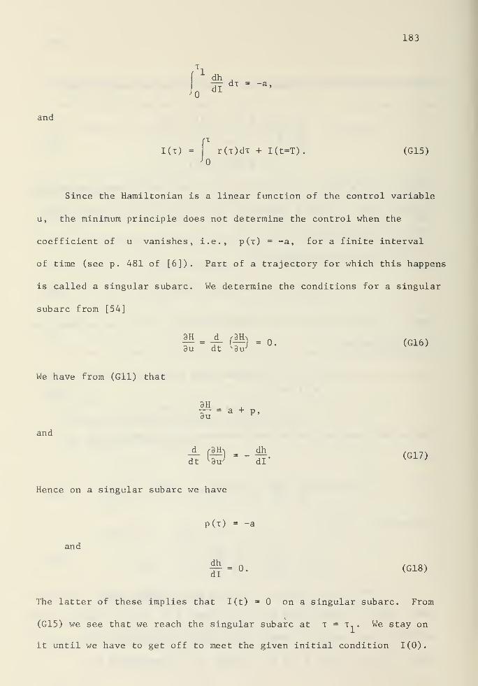
183

di— -

and

Kt) = r(i)dx + I(t=T). (G15)

Since the Hamiltonian is a linear function of the control variable

u, the minimum principle does not determine the control when the

coefficient of u vanishes, i.e., p(x) = -a, for a finite interval

of time (see p. 481 of [6]). Part of a trajectory for which this happens

is called a singular subarc. We determine the conditions for a singular

subarc from [54]

3H d a = 0. (G16)Bu dt v duJ

We have from (Gil) that

and

(G17)

3H

iu"= a + P '

jd_ /3H> dh

dt W =

di*

Hence on a singular subarc we have

p(x) = -a

and

ff- 0. (G18)

The latter of these implies that I(t) =0 on a singular subarc. From

(G15) we see that we reach the singular subarc at T — x, . We stay on

it until we have to get off to meet the given initial condition 1(0).

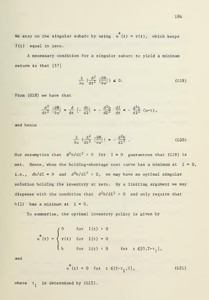
184

We stay on the singular subarc by using u (t) = r(t), which keeps

I(t) equal to zero.

A necessary condition for a singular subarc to yield a minimum

return is that [57]

From (G18) we have that

d2 r3H^ d

fdh^ d2h dl d2h , N

dt2" W =

dT r dfJ= " dT* dT

=" dF (u_r)

»

and hence

3 . d2f3Hn .

d 2h

iu~{dt^" W } ' " dl* *

(G20)

Our assumption that d 2h/dl 2 > for 1=0 guarantees that (G19) is

met. Hence, when the holding-shortage cost curve has a minimum at 1=0,

i.e., dh/dl = and d2h/dl 2 > 0, we may have an optimal singular

solution holding the inventory at zero. By a limiting argument we may

dispense with the condition that d 2h/dl 2 > and only require that

h(I) has a minimum at 1=0.

To summarize, the optimal inventory policy is given by

for I(t) >

u*(t) = < r(t) for I(t) =

and

for I(t) < for t €[0,T-t ],

u*(t) =0 for t ^(T-x1,T], (G21)

where T- is determined by (G15)

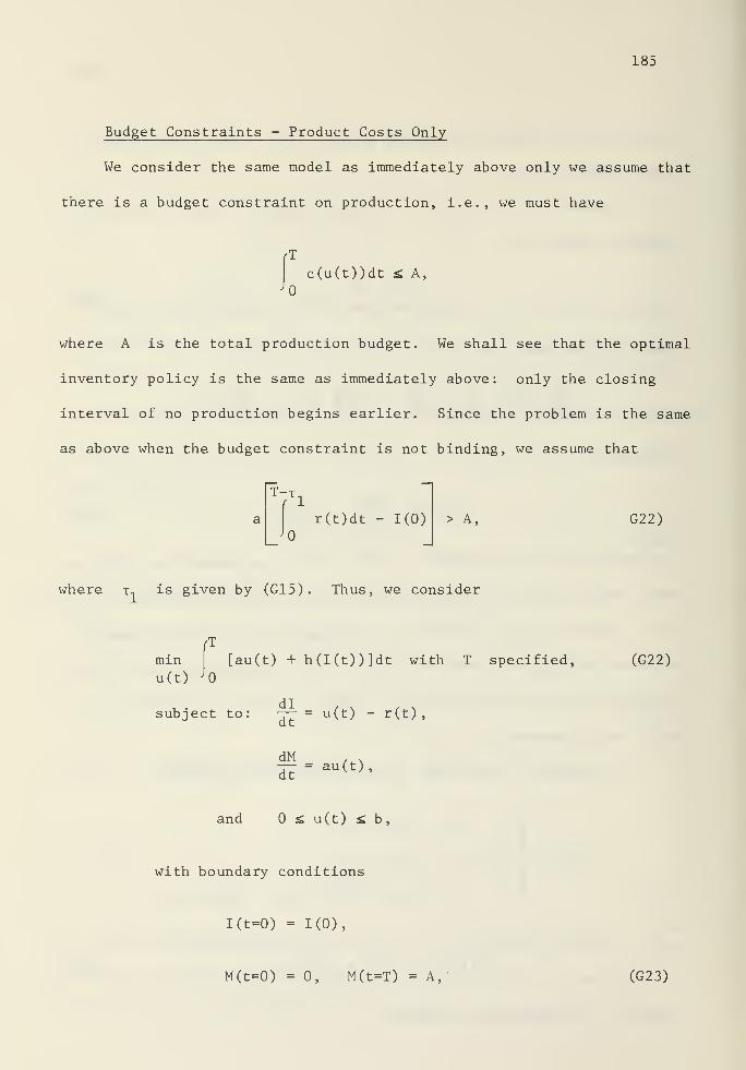
185

Budget Constraints - Product Costs Only

We consider the same model as immediately above only we assume that

there is a budget constraint on production, i.e., we must have

c(u(t))dt «; A,

where A is the total production budget. We shall see that the optimal

inventory policy is the same as immediately above: only the closing

interval of no production begins earlier. Since the problem is the same

as above when the budget constraint is not binding, we assume that

T7Ti

r(t)dt - 1(0) > A, G22)

where t, is given by (G15) . Thus, we consider

fT

mmu(t)

[au(t) +h(I(t))]dt with T specified.

dlsubject to: -j— = u(t) - r(t),

dMdt

= au(t),

(G22)

and <£ u(t) £ b,

with boundary conditions

l(t=0) = 1(0),

M(t=0) = 0, M(t=T) = A, (G23)

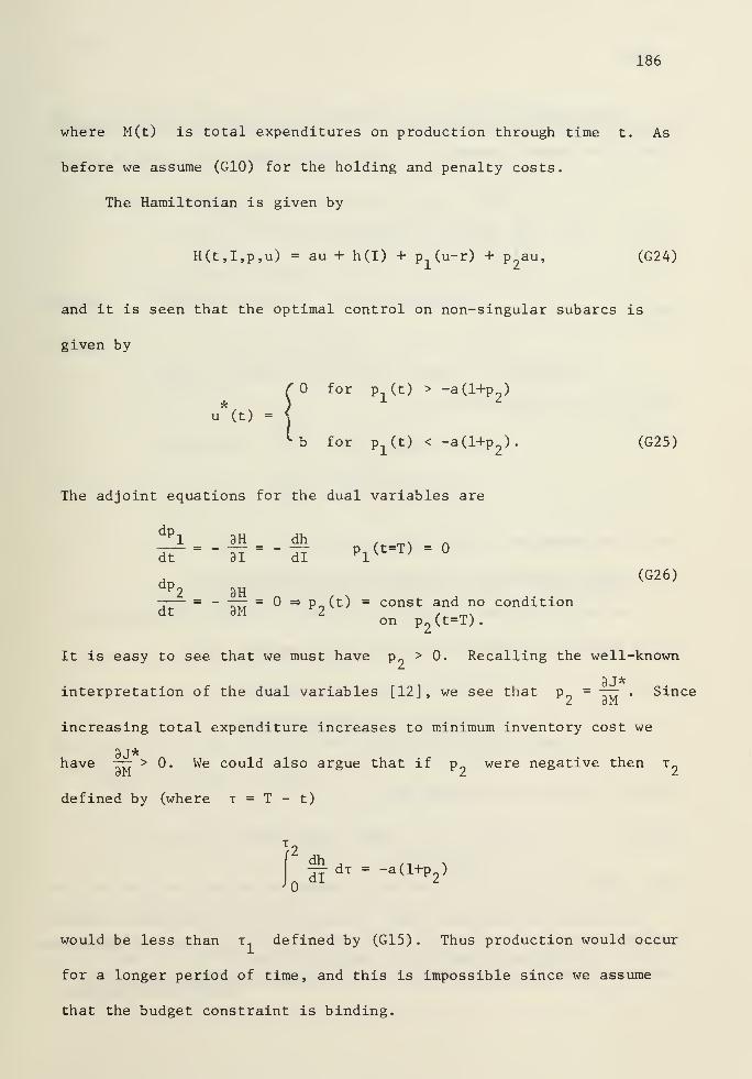
186

where M(t) is total expenditures on production through time t. As

before we assume (G10) for the holding and penalty costs.

The Hamiltonian is given by

H(t,I,p,u) = au + h(I) + p^u-r) + p2au, (G24)

and it is seen that the optimal control on non-singular subarcs is

given by

for p (t) > -a(l+p )

* i z

u (t) =

b for Pl (t) < -a(l+p2). (G25)

The adjoint equations for the dual variables are

dPl 3H dh p,<«)-0dt 31 dl

dPo(G26)

= =* p„(t) = const and no conditiondt 3M r

2on p

2(t=T).

It is easy to see that we must have p > 0. Recalling the well-known

3J*interpretation of the dual variables [12], we see that p_ = — . Since

2 3M

increasing total expenditure increases to minimum inventory cost we

3J*have — > 0. We could also argue that if p n were negative then x_

3M 2 2

defined by (where t = T - t)

qf dx - -a(l+p

2)

would be less than x defined by (G15). Thus production would occur

for a longer period of time, and this is impossible since we assume

that the budget constraint is binding.

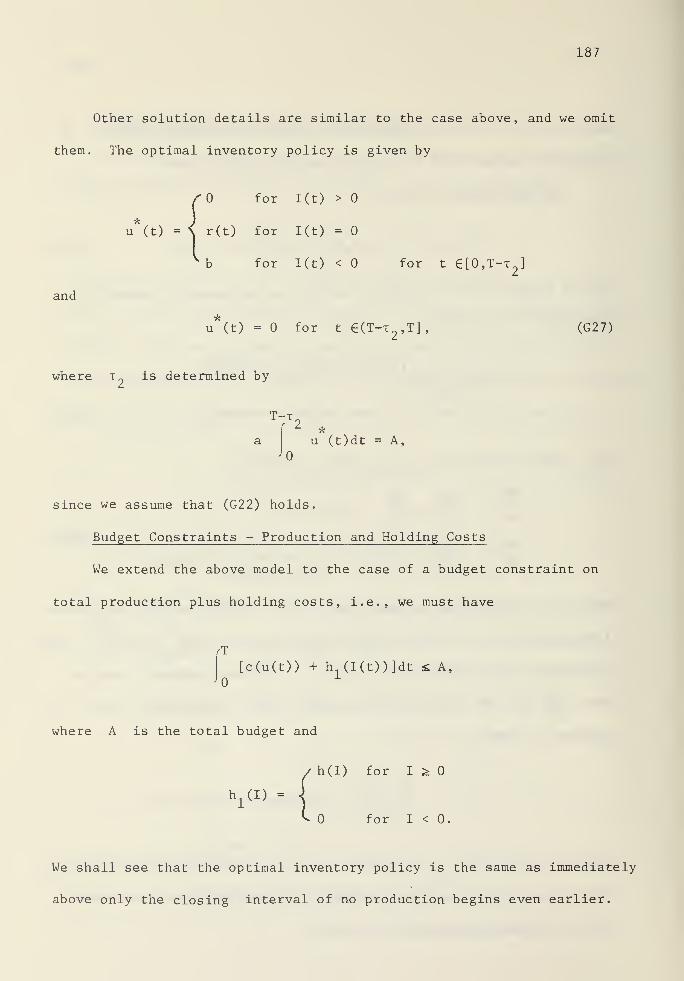
187

Other solution details are similar to the case above, and we omit

them. The optimal inventory policy is given by

for I(t) >

)

u (t) = < r(t) for I(t) =

and

for I(t) < for t €[0,T-t ]

u*(t) =0 for t €(T-t2,T], (G27)

where t?

is determined by

T-xr 2 *

u (t)dt = A,

since we assume that (G22) holds.

Budget Constraints - Production and Holding Costs

We extend the above model to the case of a budget constraint on

total production plus holding costs, i.e., we must have

[c(u(t)) + h (I(t))]dt <; A,

where A is the total budget and

h(I) for I ;>

h1(I) =

for I <

We shall see that the optimal inventory policy is the same as immediately

above only the closing interval of no production begins even earlier.

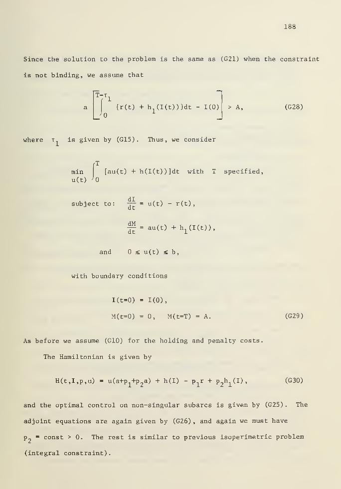
188

Since the solution to the problem is the same as (G21) when the constraint

is not binding, we assume that

T-T.

{r(t) + h1(I(t))}dt - 1(0) > A, (G28)

where x is given by (G15) . Thus, we consider

mmu(t)

[au(t) + h(I(t))]dt with T specified,

, . dl , N , .

subject to: — = u(t) - r(t),

dM.= au(t) + h

1(I(t)),

and £ u(t) s: b,

with boundary conditions

l(t=0) = 1(0),

M(t=0) - 0, M(t=T) = A. (G29)

As before we assume (G10) for the holding and penalty costs

The Hamiltonian is given by

H(t,I,p,u) = u(a+Pl+p 2a) + h(I) - p^ + P^U) ,

(G30)

and the optimal control on non-singular subarcs is given by (G25). The

adjoint equations are again given by (G26) , and again we must have

p 9= const > 0. The rest is similar to previous isoperimetric problem

(integral constraint)

.

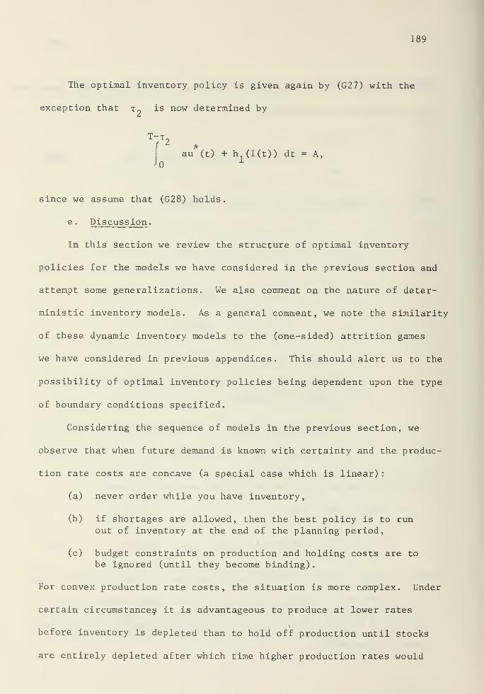
189

The optimal inventory policy is given again by (G27) with the

exception that t 9is now determined by

Y*au*(t) + h (I(t)) dt = A,

since we assume that (G28) holds.

e . Discussion .

In this section we review the structure of optimal inventory

policies for the models we have considered in the previous section and

attempt some generalizations. We also comment on the nature of deter-

ministic inventory models. As a general comment, we note the similarity

of these dynamic inventory models to the (one-sided) attrition games

we have considered in previous appendices. This should alert us to the

possibility of optimal inventory policies being dependent upon the type

of boundary conditions specified.

Considering the sequence of models in the previous section, we

observe that when future demand is known with certainty and the produc-

tion rate costs are concave (a special case which is linear)

:

(a) never order while you have inventory,

(b) if shortages are allowed, then the best policy is to runout of inventory at the end of the planning period,

(c) budget constraints on production and holding costs are to

be ignored (until they become binding).

For convex production rate costs, the situation is more complex. Under

certain circumstances it is advantageous to produce at lower rates

before inventory is depleted than to hold off production until stocks

are entirely depleted after which time higher production rates would

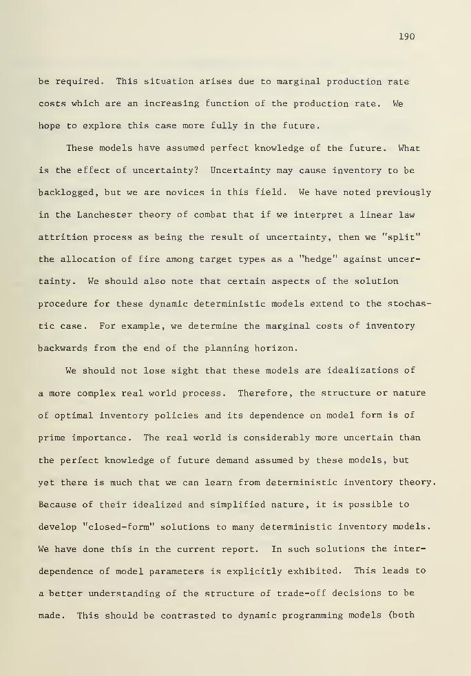
190

be required. This situation arises due to marginal production rate

costs which are an increasing function of the production rate. We

hope to explore this case more fully in the future.

These models have assumed perfect knowledge of the future. What

is the effect of uncertainty? Uncertainty may cause inventory to be

backlogged, but we are novices in this field. We have noted previously

in the Lanchester theory of combat that if we interpret a linear law

attrition process as being the result of uncertainty, then we "split"

the allocation of fire among target types as a "hedge" against uncer-

tainty. We should also note that certain aspects of the solution

procedure for these dynamic deterministic models extend to the stochas-

tic case. For example, we determine the marginal costs of inventory

backwards from the end of the planning horizon.

We should not lose sight that these models are idealizations of

a more complex real world process. Therefore, the structure or nature

of optimal inventory policies and its dependence on model form is of

prime importance. The real world is considerably more uncertain than

the perfect knowledge of future demand assumed by these models, but

yet there is much that we can learn from deterministic inventory theory,

Because of their idealized and simplified nature, it is possible to

develop "closed-form" solutions to many deterministic inventory models.

We have done this in the current report. In such solutions the inter-

dependence of model parameters is explicitly exhibited. This leads to

a better understanding of the structure of trade-off decisions to be

made. This should be contrasted to dynamic programming models (both

191

deterministic and probabilistic) for which, in most instances, a solution

is developed only for a specific set of parameter values. In this case,

it is difficult (if not impossible) to see the structure of optimal

inventory policies and its dependence on model form without a parametric

analysis of model output.

The intimate connection between variational methods and dynamic

programming (their dual relationship in the sense of J. Plucker's

principle of duality ) is well known [10], [30]. It is important to

understand the Hamilton-Jacobi approach to variational problems. In

discrete and stochastic cases, we formulate the analogue of the Hamil-

ton-Jacobi-Bellman equation for the optimal return. Hence, understanding

the principles of the solution procedure in the deterministic case pro-

vides the insight for extensions.

Actually first stated in non-algebraic terms by J. Gergonne.

192

REFERENCES

1. R. Ackoff, Scientific Method : Optimizing Applied Research Decisions ,

John Wiley & Sons, New York (1962).

2. I. Adiri and A. Ben-Israel, "An Extension and Solution of Arrow-KarlinType Production Models by the Pontryagin Maximum Prinicple," Cashiersde Recherche Operationelle , 8, 147-158 (1966).

3. K. Arrow and S. Karlin, "Production over Time with Increasing MarginalCosts," Chapter 4 in Studies in the Mathematical Theory of Inventoryand Production , K. Arrow, S. Karlin and H. Scarf, Stanford UniversityPress, Stanford, California (1958).

4. K. Arrow, S. Karlin and H. Scarf, Studies in the Mathematical Theoryof Inventory and Production , Stanford University Press, Stanford,California (1958).

5. M. Athans , "The Status of Optimal Control Theory and Applications for

Deterministic Systems," IEEE Trans, on Automatic Control , Vol. AC-11,580-596 (1966).

6. M. Athans and P. Falb , Optimal Control , McGraw-Hill, New York (1966).

7. R. Bach, L. Dolansky and H. Stubbs, "Some Recent Contributions to the

Lanchester Theory of Combat," Opns. Res ., 10, 314-326 (1962).

8. A. Balakrishnan and L. Neustadt, (Ed.), Mathematical Theory of Control,

Academic Press, New York (1967).

9. R. Bellman, Dynamic Programming , Princeton University Press,Princeton (1957).

10. R. Bellman and S. Dreyfus, Applied Dynamic Programming , PrincetonUniversity Press, Princeton (1962).

11. L. D. Berkovitz, "A Differential Game with No Pure Strategy Solution,"Annals of Mathematics Study , No. 52, Princeton, 175-194 (1964).

12. , "Necessary Conditions for Optimal Strategies in a Class of

Differential Games and Control Problems," SIAM J. Control , 5, 1-24 (1967)

13. , "A Survey of Differential Games," in Mathematical Theoryof Control , A. Balakrishnan and L. Neustadt (Ed.), Academic Press,New York (1967).

14. L. D. Berkovitz and M. Dresher, "A Game Theory Analysis of Tactical AirWar." Opns. Res . , 7, 599-620 (1959).

193

15. , "Allocation of Two Types of Aircraft in Tactical Air War:A Game Theoretic Analysis," Opns . Res ., 8, 694-706 (1960).

16. A. Blaquiere, F. Gerard and G. Leitman: Quantitative and QualitativeGames , Academic Press, New York (1969).

17. G. Bliss, "The Use of Adjoint Systems in the Problems of DifferentialCorrections for Trajectories," Journal of the United States Artillery

,

51, 445-449 (1919).

18. 0. Bolza, Lectures on the Calculus of Variations , University of ChicagoPress, Chicago, Illinois (1904) (also available as Dover reprint).

19. S. Bonder, "Combat Model," Chapter 2 in The Tank Weapon System , ReportNo. RF 573 AR 64-1 (U) , Systems Research Group, The Ohio State University(1964).

20. , "A Theory for Weapon System Analysis," Proceedings U. S .

Army Operations Research Symposium , 111-128 (1965).

21. , "The Lanchester Attrition-Rate Coefficient," Opns. Res .

,

15, 221-232 (1967).

22. H. Brackney, "The Dynamics of Military Combat," Opns. Res . , 7, 30-44

(1959).

23. R. H. Brown, "Theory of Combat: The Probability of Winning," Opns. Res .

,

11, 418-425 (1963).

24. A. Bryson and Y. C. Ho, Applied Optimal Control , Blaisdell PublishingCompany, Waltham, Massachusetts (1969).

25. J. Case, "Summary of the Lectures Presented at the Workshop onDifferential Games." Held at Madison, Wisconsin, June 24-28, 1968,under the Auspices of the Mathematics Steering Committee of the UnitedStates Army (unpublished).

26. C. Churchman, R. Ackoff and E. Arnoff, Introduction to OperationsResearch , John Wiley, New York (1957).

27. R. Courant and D. Hilbert, Methods of Mathematical Physics , Vol. II,

Interscience, New York (1962).

28. L. Dolansky, "Present State of the Lanchester Theory of Combat," Opns .

Res., 12, 344-358 (1964).

29. M. Dresher, Games of Strategy , Prentice-Hall, Englewood Cliffs, NewJersey (1961).

194

30. S. Dreyfus, Dynamic Programming and the Calculus of Variations , AcademicPress, New York (1965).

31. A. Eckler, "A Survey of Coverage Problems Associated with Point and AreaTargets," Technometrics , 11, 561-589 (1969).

32. 0. Elgerd, Control Systems Theory , McGraw-Hill, New York (1967).

33. L. Fan, The Continuous Maximum Principle , John Wiley, New York (1966).

34. D. Fulkerson and S. Johnson, "A Tactical Air Game," Opns . Res . , 5,

704-712 (1957).

35. D. Gilliland, "Integral of the Bivariate Normal Distribution over anOffset Circle," J. Amer. Statist. Assoc , 57, 758-767 (1962).

36. F. Grubbs, "Approximate Circular and Noncircular Offset Probabilitiesof Hitting, Opns. Res . , 12, 51-62 (1964).

37. R. Helmbold, "Some Observations on the Use of Lanchester's Theory for

Prediction," Opns. Res ., 12, 778-781 (1964).

38. , "A Modification of Lanchester's Equations," Opns . Res . , 13,

857-859 (1965).

39. , "A 'Universal' Attrition Model," Opns. Res ., 14, 624-635

(1966).

40. F. Hildebrand, Advanced Calculus for Engineers , Prentice-Hall, New York(1948).

41. Y. C. Ho, "Review of the Book Differential Games by R. Isaacs," IEEE

Trans, on Automatic Control , Vol. AC-10, 501-503 (1965).

42. , "Toward Generalized Control Theory," IEEE Trans, on

Automatic Control , Vol. AC-14, 753-754 (1969).

43. , "The First International Conference on the Theory and

Applications of Differential Games," FINAL REPORT, Division of Engineeringand Applied Physics, Harvard University, Cambridge, Massachusetts,January 1970.

44. Y. C. Ho, A. Bryson and S. Baron, "Differential Games and Optimal Pursuit-

Evasion Strategies," IEEE Trans, on Automatic Control , Vol. AC-10,385-389 (1965).

45. E. Ince, Ordinary Differential Equations , Dover Publications, New York

(1944).

195

46. R. Isaacs, "Differential Games I: Introduction," RM-1391, The RANDCorporation (1954).

47. , "Differential Games II: The Definition and Formulation,"RM-1399, The RAND Corporation (1954).

48. , "Differential Games III: The Basic Principles of theSolution Process," RM-1411, The RAND Corporation (1954).

49. , "Differential Games IV: Mainly Examples," RM-1486, TheRAND Corporation (1955).

50. , Differential Games , John Wiley, New York (1965).

51. J. Isbell and W. Marlow, "Attrition Games," Naval Res. Log. Quart ., 3,

71-94 (1956).

52. , "Methods of Mathematical Tactics," Logistics Papers , No. 14,The George Washington University Logistics Research Project, September1956.

53. C. Johnson, "Singular Solutions in Problems of Optimal Control," in

Advances in Control Systems , Vol. 2, C. Leondes (Ed.), Academic Press,

New York (1965).

54. C. Johnson and J. E. Gibson, "Singular Solutions in Problems of OptimalControl," IEEE Trans, on Automatic Control , Vol. AC-8, 4-15 (1963).

55. S. Karlin, Mathematical Methods and Theory in Games, Programming, andEconomics , Vol. 2, John Wiley, New York (1959).

56. , "The Mathematical Theory of Inventory Processes," Chapter10 in Modern Mathematics for the Engineer , E. Beckenbach (Ed.), McGraw-Hill,New York (1961).

57. H. Kelley, R. Kopp and H. Moyer, "Singular Extremals," in Topics in

Optimization , G. Leitman (Ed.), Academic Press, New York (1967).

58. T. Kisi and Y. Kawahara, "A Target Assignment Problem." Paper Presentedat the ORAW Meeting, Tokyo, Japan, August 18, 1967.

59. B. Klein, "Direct Use of Extremal Principles in Solving CertainOptimizing Problems Involving Inequalities," Opns. Res . , 3, 168-175

(1955).

60. B. Koopman, "Logical Basis of Combat Simulation," Columbia University,Mathematics Department Report (1968).

61. F. W. Lanchester, Aircraft in Warfare; The Dawn of the Fourth Arm,

Constable, London (1916).

196

62. C. Lanczos, Linear Differential Operators , Von Nostrand, London (1961).

63. A. McMasters, "Optimal Control in Deterministic Inventory Models."Report, U. S. Naval Postgraduate School, Monterey, California (1970).

64. F. Morin, "Note on an Inventory Problem," Econometrica , 23, 447-450(1955).

65. P. Morse and H. Feshback, Methods of Theoretical Physics , McGraw-Hill,New York (1953).

66. P. Morse and G. Kimball, Methods of Operations Research , M.I.T. Press,Cambridge, Massachusetts (1951).

67. f. Moulton, Methods in Exterior Ballistics , University of Chicago Press,Chicago (1926) (also available as Dover reprint).

68. L. Pontryagin, Y. Boltyanski, R. Gamkrelidze and E. Mishchenko, TheMathematical Theory of Optimal Processes , Interscience Publishers, Inc.,

New York (1962).

69. H. Sagan, Introduction to the Calculus of Variations , McGraw-Hill, NewYork (1969).

70. T. Schreiber, "Note on the Combat Value of Intelligence and CommandControl Systems," Opns. Res . , 12, 507-510 (1960).

71. E. Simakova, "Differential Games," Automation and Remote Control , 27,

1980-1998 (1967) (English translation from Avtomatika i Telemekhanika,

27, 161-178 (1966).

72. R. Snow, "Contributions to Lanchester Attrition Theory," The RAND

Corporation, Report RA-15078 (1948).

'73. Systems Research Laboratory, Department of Industrial Engineering,"Development of Models for Defense Systems Planning," Report NumberSRL 2147, SA 69-1, University of Michigan, Ann Arbor, Michigan, March1969.

74. J. Taylor, "Comments on Some Differential Games of Tactical Interest."Paper Presented March 20, 1970 at Spring Meeting Operations ResearchSociety of America (San Diego Section).

75., "Lanchester-Type Models of Warfare and Optimal Control."

Paper Presented April 21, 1970 at 37th National Meeting OperationsResearch Society of America.

76.5 "Application of Differential Games to Problems of Naval War-

fare: Surveillance-Evasion - Part I." Report, U. S. Naval PostgraduateSchool, Monterey, California (1970).

19 7

77. G. Tracz, "A Selected Bibliography on the Application of Optimal ControlTheory to Economic and Business Systems, Management Science andOperations Reserach," Opns. Res . , 16, 174-186 (1968).

78. J. von Neumann and 0. Morgenstern, Theory of Games and Economic Behavior,

Princeton University Press, Princeton (1944).

79. G. Watson, A Treatise on the Theory of Bessel Functions , 2nd Ed.,

University Press, Cambridge (1945).

80. H. K. Weiss, "Requirements for a Theory of Combat; Lanchester Models,"BRL Report No. 667 (1953).

81. , "Lanchester-Type Models of Warfare," Proc. First InternationalCont. Operational Res., Oxford (1957).

82. » "Some Differential Games of Tactical Interest and the Valueof a Supporting Weapon System," Opns. Res . , 7, 180-196 (1959).

83. , "Stochastic Models for the Duration and Magnitude of a

'Deadly Quarrel'," Opns. Res . , 11, 101-121 (1963).

198

INITIAL DISTRIBUTION LIST

No. of copies

Defense Documentation Center (DDC) 20Cameron StationAlexandria, Virginia 22314

Library 2

Naval Postgraduate SchoolMonterey, California 93940

Dean of Research Administration 2

Code 023Naval Postgraduate SchoolMonterey, California 93940

The Office of Naval Research 2

Code 462Washington, D. C.

Central Files 1

Naval Postgraduate SchoolMonterey, California 93940

Professor Frank Faulkner 1

Department of MathematicsNaval Postgraduate SchoolMonterey, California 93940

Professor Peter W. Zehna 1

Department of Operations AnalysisNaval Postgraduate SchoolMonterey, California 93940

Dr. Jong-Sen Lee 1

Naval Research LaboratoryDepartment of the NavyWashington, D. C. 20390

Mr. H. K. Weiss 1

P. 0. Box 2668Palos Verdes PeninsulaPalos Verdes, California 90274

Dean J. G. Debanne 1

Faculty of Management SciencesUniversity of OttawaOttawa 2, Canada

199

Professor B. 0. Koopman 1

Department of MathematicsColumbia UniversityNew York, New York 10027

Mr. L. Ostermann 1

Lule j ian and Associates, Inc.

1650 S. Pacific Coast HighwayRedondo Beach, California

Professor James G. Taylor 30

Department of Operations AnalysisNaval Postgraduate SchoolMonterey, California 93940

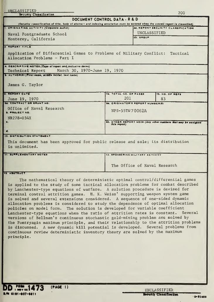
UNCLASSIFIEDSecurity Classification 200

DOCUMENT CONTROL DATA R&D(Security clatalllcatlon ot title, body ot abstract and Indexing annotation mull be entered when the overall report la elaaalHad)

I originating ACTIVITY (Corporal* author)

Naval Postgraduate SchoolMonterey, California

la. REPORT SECURITY CLASSIFICATION

UNCLASSIFIED2b. 8KOUP

J REPORT TITLE

Application of Differential Games to Problems of Military ConflictAllocation Problems - Part I

Tactical

4. OESCRIRTIVK NOTE! (Type ot report and, Incluatv daft)

Technical Report March 30, 1970-June 19, 1970S auThorisi (Flrat name, middle Initial, laat name)

James G. Taylor

• REPORT DATE

June 19, 1970

7a. TOTAL NO. OP PASES

2017b. NO. OP REPS

83M. CONTRACT OR ORANT NO.

Office of Naval Researchb. PROJECT NO.

NR278-034X

M. ORIGINATOR'S REPORT NUMBERISI

NPS-55TW7 0062A

•b. OTHER REPORT NOIS) (Any other number* that may me aa alinedthla report)

• 0. DISTRIBUTION STATEMENT

This document has been approved for public release and sale; its distributionis unlimited.

II. SUPPLEMENTARY NOTES 12. SPONSORING MILITARY ACTIVITY

The Office of Naval Research

IS. ABSTRACT

The mathematical theory of deterministic optimal control/differential games

is applied to the study of some tactical allocation problems for combat described

by Lanchester-type equations of warfare. A solution procedure is devised for

terminal control attrition games. H. K. Weiss' supporting weapon system game

is solved and several extensions considered. A sequence of one-sided dynamic

allocation problems is considered to study the dependence of optimal allocation

policies on model form. The solution is developed for variable coefficient

Lanchester-type equations when the ratio of attrition rates is constant. Several

versions of Bellman's continuous stochastic gold-mining problem are solved by

the Pontryagin maximum principle, and their relationship to the attrition problems

is discussed. A new dynamic kill potential is developed. Several problems from

continuous review deterministic inventory theory are solved by the maximum

principle.

DD ,'r..1473t/M 01 01 -107 •«• It

(PAGE 1)UNCLASSIFIED

kttirlty CUssInostU*~»i«ot

UNCLASSIFIEDSecurity Classification 201

K I V WO KDI

Differential Games

Tactical Allocation

Command Control

Military Tactics

Lanchester Theory of Combat

Dynamic Kill Potential

Inventory Theory

HOLE

.

DD ,'°.?..1473 <«*>~~h. **

S/N 0101 -807-SJ21UNCLASSIFIEDSecurity Classification A- 3 1 409

13636

DUDLEY KNOX LIBRARY - RESEARCH REPORTS

5 6853 058201 8

_ ,

mv