Unit 2-Background of Classification, Pattern …pattern-recognition.weebly.com/uploads/4/0/1/0/40109209/...• Classification step: given a new pattern with unknown class (one large

1

• This is the second lecture note of the course PATTERN

RECOGNITION in English in 104-2 semester, EE, FJU.

• In this lecture note, I will introduce mathematical basics

classification.

• Web site of this course: http://pattern-recognition.weebly.com.

2

3

4

5

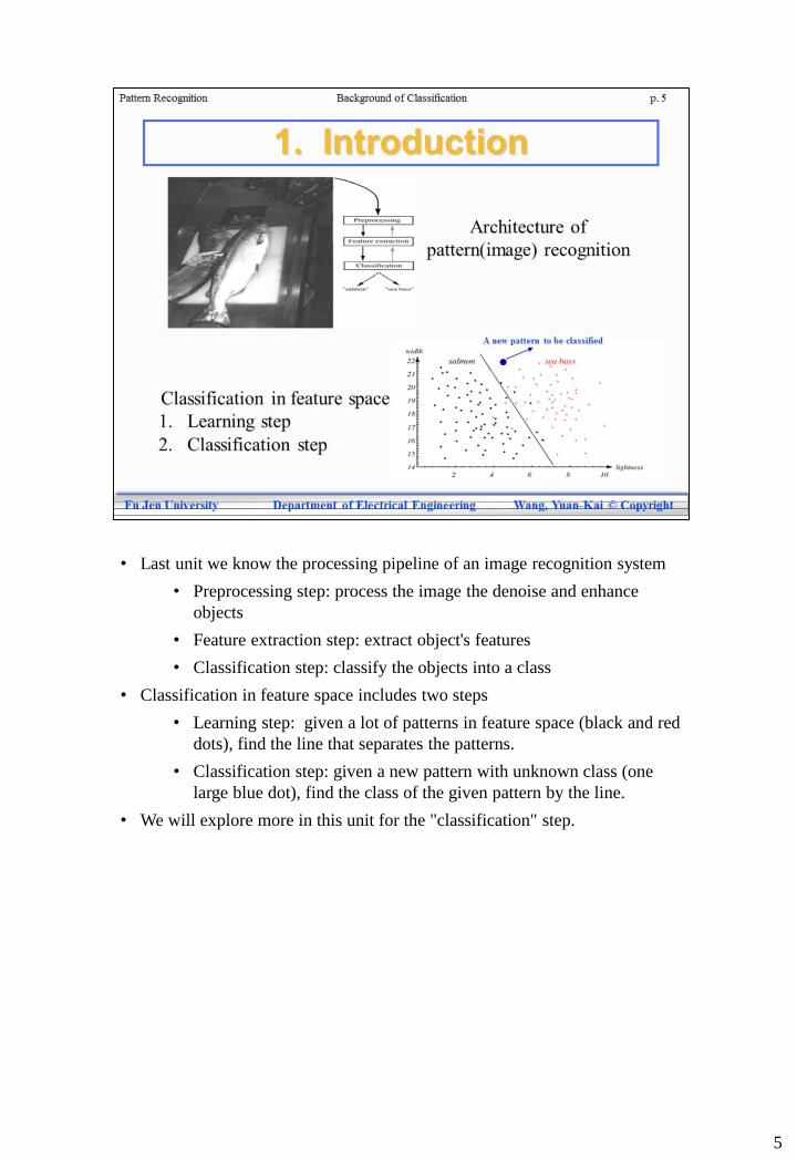
• Last unit we know the processing pipeline of an image recognition system

• Preprocessing step: process the image the denoise and enhance

objects

• Feature extraction step: extract object's features

• Classification step: classify the objects into a class

• Classification in feature space includes two steps

• Learning step: given a lot of patterns in feature space (black and red

dots), find the line that separates the patterns.

• Classification step: given a new pattern with unknown class (one

large blue dot), find the class of the given pattern by the line.

• We will explore more in this unit for the "classification" step.

• We classify image objects, such as fishes and faces, by their distribution in

an algebraic space called feature space.

• Although practically fish classification and face recognition are

different problems

• Theoretically we think they are the same problem: classify objects in

their feature spaces

• In this feature space with a two-class problem

• Each axis represents a feature

• Each dot represents an image object

• A class of image objects is assumed to be clustered in a region

• A class consists a set of object patterns/object points

• A line/curve is called a classifier (or a classification method) if it

separates the space into two regions and separates the image objects

into two sets.

6

• In this unit, we will explore concepts and terminologies of classification in

feature space

• First I will explain "feature space" in Section 2

• Section 3 gives some examples of patterns in feature space

• Linear patterns

• Nonlinear patters

• Section 4 explains classifier as discriminants.

• The straight line separating the two classes is called : discriminant,

or classifier

• The concept of minimum distance classifier is also introduced.

• Section 5 explains machine learning for pattern recognition.

7

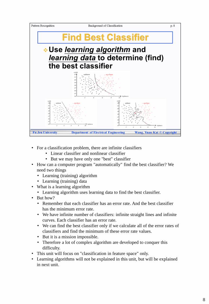
• For a classification problem, there are infinite classifiers

• Linear classifier and nonlinear classifier

• But we may have only one "best" classifier

• How can a computer program "automatically" find the best classifier? We

need two things

• Learning (training) algorithm

• Learning (training) data

• What is a learning algorithm

• Learning algorithm uses learning data to find the best classifier.

• But how?

• Remember that each classifier has an error rate. And the best classifier

has the minimum error rate.

• We have infinite number of classifiers: infinite straight lines and infinite

curves. Each classifier has an error rate.

• We can find the best classifier only if we calculate all of the error rates of

classifiers and find the minimum of these error rate values.

• But it is a mission impossible.

• Therefore a lot of complex algorithm are developed to conquer this

difficulty.

• This unit will focus on "classification in feature space" only.

• Learning algorithms will not be explained in this unit, but will be explained

in next unit.

8

9

• This section will explain what is feature space.

10

• A feature vector p1 is a point in a d-dimension pattern space.

• Each element of the vector is a feature, and each one corresponds to one

dimension (axis) in the space.

• In the fish classification example, we have only two features

• The feature space is a 2-dimensional space: d=2.

• Each fish is denoted as p1.

11

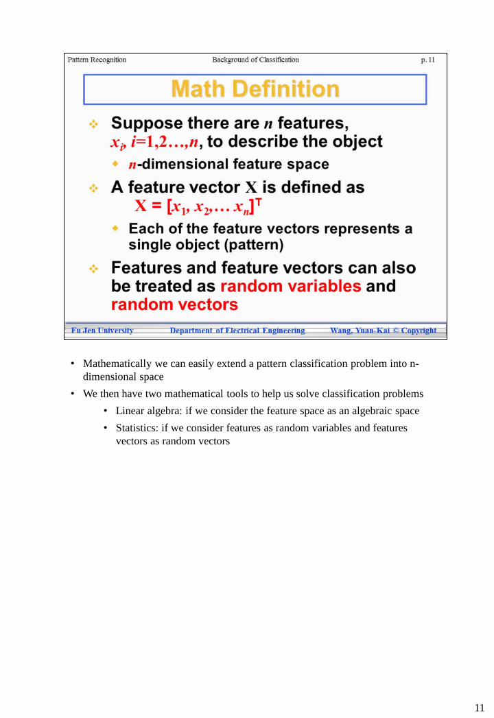
• Mathematically we can easily extend a pattern classification problem into n-

dimensional space

• We then have two mathematical tools to help us solve classification problems

• Linear algebra: if we consider the feature space as an algebraic space

• Statistics: if we consider features as random variables and features

vectors as random vectors

• 2D with 2 classes is a standard case that is only used for concept

explanation

• It is easy to demonstrate basic concepts of pattern recognition

• But standard cases are only toy examples but not real-case examples

• Sometimes we will show real-case examples

• Ex.: 2D with more than two classes, 3D with two or more than two

classes.

12

• Three subsections in Section 3

• 3.1 Linearly separable patterns

• 3.2 Piecewise-linear separable patterns

• 3.3 Nonlinearly separable patterns• A class consists a set of object patterns/object points

• Separable patterns means that there exist lines, curves or hyperplanes that

discriminate the classes

• Linearly separable patterns belong to linear classification problem.

• Linear => straight line (2D), because a straight line is a linear

function

• Linear => plane (3D), because a plane is also a linear function

• For more than 3D cases, linear => hyperplane.

• All first-order polynomials are linear

• Nonlinearly separable patterns belong to nonlinear classification problem.

• Circle is a nonlinear function

• Ellipse is a nonlinear function

• Parabola and hyperbolic curves are nonlinear functions

• All high-order polynomials are nonlinear

13

• Here we can see three examples of linearly separable patterns

• The first row has two 2D examples

• The second row shows a 3D example

• In a 2D space, the line to linearly separate classes are called a linear

classifier

• The classifier can be described by ax + by +c = 0, if the x1 is

regarded as x, and x2 is regarded as y.

• The classifier is also called a decision surface, decision line, or

decision boundary.

• In a 3D space, the plane to linearly separate classes are still called a linear

classifier

• A plane can still be described by a linear formula:

ax + by + cz + d = 0.

14

• Patterns in feature space are usually not linearly separable

• Here we give some examples of nonlinearly separable patterns

• Piecewise linearly separable

• Circularly separable

• XOR

• Unclear boundary

• Piecewise linearly separable

• Classes can not be separated by only one lines, but can be separated

by more lines (pieces of lines).

• Circularly separable

• Classes have clear boundary, but they can not be separated by lines.

Circle or ellipse can be used to separate these two classes.

• XOR

• Two classes, red and blue, can not be separated by any linear

formulas.

• This is a very famous case for pattern classification. Later we may

see more discussions of this XOR case.

• Unclear boundary (for the fish classification example)

• The previous three examples are nonlinear but with clear boundary

between classes.

• For the fish classification example, there is no clear boundary

between two classes. Therefore a line is not able to separate the two

classes.

• This example is very close to many real cases in pattern recognition

systems. More advanced pattern recognition algorithms are

proposed for this kind of nonlinearity.

15

16

• For this example, both linear discriminant and nonlinear discriminant can

separate patterns

• C1 region represents a lot of pattern points that belong to the class 1

• C2 region represents a lot of pattern points that belong to the class 2

• The line x-y=0 can separate the two classes

• A parabola can also separate the two classes

• However

• This example should be called a linear separable example

• That is, if "at least one" linear discriminant exists for the example,

then the example should be called "linear separable"

17

• For this 3-class example, it is called nonlinearly separable, because

• No linear discriminants exist to separate classes 2 and 3.

• Only nonlinear discriminants can solve this example.

• Linear discriminants are easier than nonlinear discriminants

• Always use linear discriminants first to separate patterns

• If it is not possible to use linear discriminants, then we still can use

nonlinear discriminants

18

19

• Piecewise-linear discrimination:

• The study of linear discrimination in the past was very popular in

academic circles because it was easy to produce iterative learning

algorithms.

• So, in the early years of PR research a great deal of attention was

devoted to separable problems.

• Separable problems are the problems in which

discriminants could be found that gave error-free

separation of points in pattern space.

• However, piecewise-linear discrimination

• is used only in simulation presented in classroom explanation.

• is useless in real cases because of the presence of nonconvex and

noncompact clusters.

• The Sebestyen problem is proposed by Sebestyen in 1962

• The problem consists 2 classes, each composed of 2 subclasses.

• No linear discriminant exists that will separate the classes.

• Sebestyen believed that the discriminant of lowest degree that will

separate them is of 6th degree.

• The XOR problem is proposed by Minsky in 196x.

• The problem consists 2 classes, each composed of 2 points.

• The XOR is a very simple case of the sebestyen problem: each

cluster has only one point.

• It is called XOR because it corresponds to the XOR logic operation

• 0 XOR 0 gets 0

• 1 XOR 1 gets 0

• 1 XOR 0 gets 1

• 0 XOR 1 gets 1

• If we consider the simple XOR logic operation to be a pattern

classification problem

• It is actually not a simple PR problem.

• It can not be solved by linear separation, but only by

piecewise or nonlinear separation.

20

21

• Piecewise linear separation

• 2 linear discriminants can separate all of the subclasses from each other.

• Each discriminant will yield one decision, labeled in the diagram "+" or "-".

• However, nonlinear separation is also possible to separate these two problems

• Ex.: A quadratic discriminant, such as a hyperbolic parabola, is able to

separate the XOR and Sebestyen's problems

kd

bv

c

au

22 )()(

Where u=mx+ny and v=px+qy,a,b,c,d,k,m,n,p,q are constants.

22

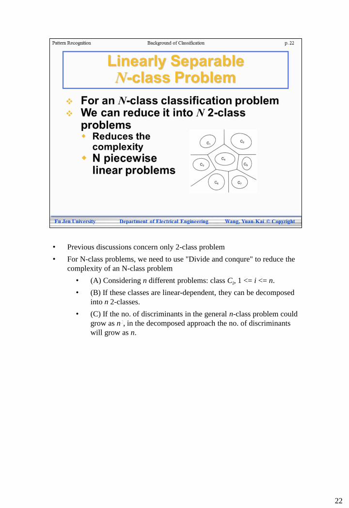
• Previous discussions concern only 2-class problem

• For N-class problems, we need to use "Divide and conqure" to reduce the

complexity of an N-class problem

• (A) Considering n different problems: class Ci, 1 <= i <= n.

• (B) If these classes are linear-dependent, they can be decomposed

into n 2-classes.

• (C) If the no. of discriminants in the general n-class problem could

grow as n2, in the decomposed approach the no. of discriminants

will grow as n.

23

• Left example: Circular patterns can not be separated by linear and

piecewise ways.

• Right example: Unclear boundary can not be separated by linear and

piecewise ways.

• Sometimes it is possible to separate unclear-boundary patterns with

piecewise linear discriminant

• But it is called overfitting and it is not good for pattern classification

• For a new pattern, the blue circle dot, it is mis-classified

• That is, although the piecewise linear lines are "perfect" for

"learning data", it is still possible tomis-classify unknown patterns.

It is not "perfect" actually.

• For a "perfect" learned classifier that is "actually not perfect", we

call it "overfitting".

• Conclusion

• For unclear boundary problems, it is nonsense to get a perfect

classifier

• All we need to get is to get a "minimum error" classifier

• Or we can use other complicated methods

24

25

• Linear separation emphasizes on "linear separability"

• It is assumed that there was no overlap of clusters of different

classes.

• However, real-world problems usually contain overlapped clusters.

• Non-separable patterns means overlapped patterns

• No perfect linear/piecewise-linear discriminant exists.

• A good way is to choose a linear/piecewise-linear discriminant

with the munimum error.

• The minimum-error discriminant

• It is usually the case that practical applications will produce

overlapping clusters.

• If it is less costly to reject rather than to make an error, we could

use the paired discriminants shown in dotted line.

• Error is usually undetected, while reject is usually processed

"manually," that is, by human being.

• Why to increase dimensions of features

• Two-class patterns in 2D may overlap and become a unclear-

boundary nonlinear problem

• Usually by adding more features, ex, add one more feature to

become a 3D feature space, those patterns become separable

• Of course, the one more feature should be more

discriminative to classify the two classes.

• How to increase the dimensions of features

• Real features

• Extract real features from images

• Simulated features

• Use mathematical ways, such as transform, to increase the

number of features.

• A very well-known method: SVM (support vector machine),

uses this way to get very good classification results for many

PR problems.

26

27

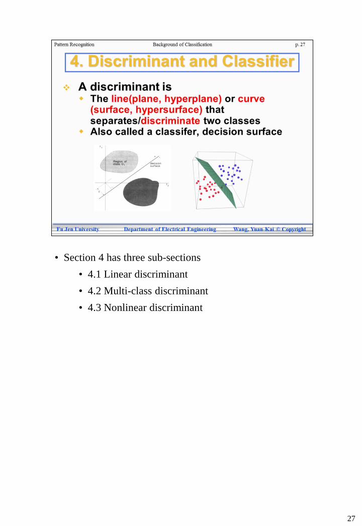
• Section 4 has three sub-sections

• 4.1 Linear discriminant

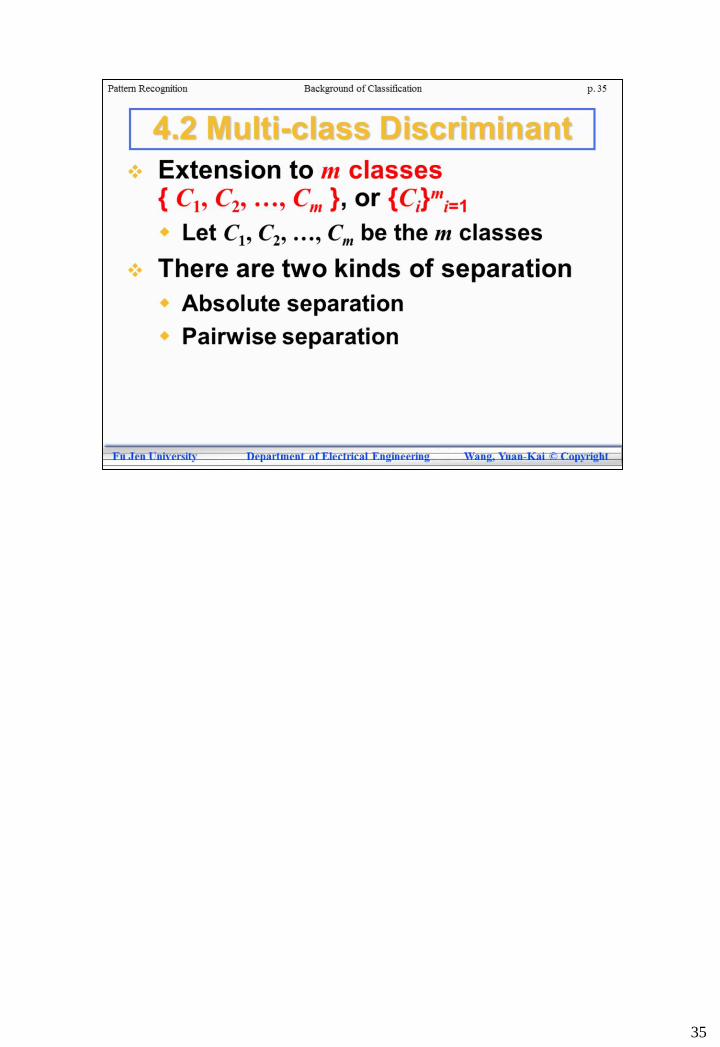
• 4.2 Multi-class discriminant

• 4.3 Nonlinear discriminant

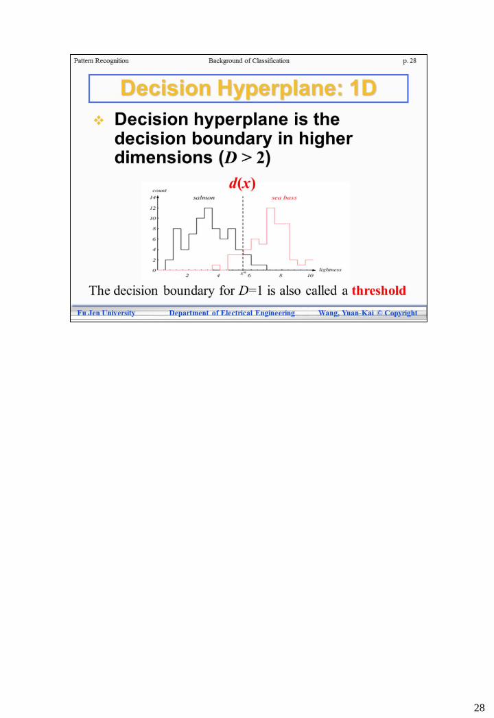
28

• Linear case

• This decision boundary is also called a "straight line"

• It is also called linear classifier, such as

• Minimum distance classifier

• Perceptron

• Nonlinear case

• This decision boundary is also called a "curve"

• It is also called nonlinear classifier

• Bayes classifier

• Support vector machines (SVM)

• Backpropogation, Decision tree, …

• For D>2, we call the

• Linear decision surface as a "decision hyperplane"

• Nonlinear decision surface as a "decision surface"

29

30

• Suppose

• Only two classes C1 and C2

• Only two features: f1 and f2

• A pattern (image object) is represented as the coordinates (f1, f2)

• The straight line to discriminate C1 and C2 is called a linear discriminant

function.

• When a hyperplane/hypersurface separates 2 clusters, the function

that defines it is called a discriminant.

• The functional form of a discriminant is an equation with

• The coefficients and variables of the space on the left side

• Zero on the right side.

• Discriminant is the locus of all points that satisfy the equation

• The best well-known linear discriminant is called "fisher" classifier.

31

• Here we extend the two-feature case (n=2) to more-feature case: n>2.

• The feature space is then extended into n-D: (x1, x2, ..., xn)

• We replace the symbol f1, f2 with x1, x2 for generalization.

• A hyperplane is a linear equation in n-dimensional space for n>2.

• Remember that a linear equation in 2D is called a straight line.

• A hyperplane is an equation, and a discriminant is an inequality.

• The slide gives a quick comparison between 2D and n-D cases. All formula

have appeared in previous two slides.

32

33

• After the understanding of discriminant with the formula of a basic form,

we want to rewrite the formula of discriminant into a matrix form.

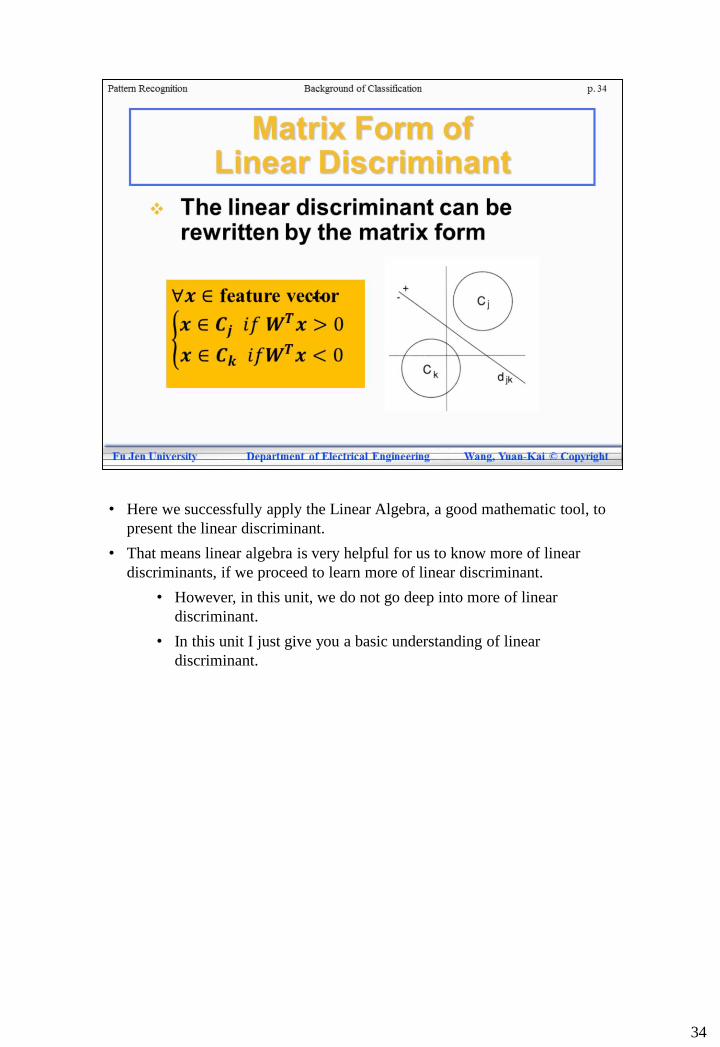
• Here we successfully apply the Linear Algebra, a good mathematic tool, to

present the linear discriminant.

• That means linear algebra is very helpful for us to know more of linear

discriminants, if we proceed to learn more of linear discriminant.

• However, in this unit, we do not go deep into more of linear

discriminant.

• In this unit I just give you a basic understanding of linear

discriminant.

34

35

36

• In the example for three classes, m=3.

• We have 3 discriminant functions d1(x), d2(x), d3(x)

• There are 3 discriminant regions

Di = { x | di(x)>0; dj(x)<0, ji }, 1 i 3

• If x locates in Di, ie. Di>0, then xCi

37

38

39

40

• There are a lot of nonlinear discriminants

• Bayesian classifier

• SVM

• NN: backpropagation, deep neural network, ...

• Adaboost

• SVM and NN are the two popular nonlinear classifiers in recent years.

41

• This is a special case of nonlinear equation d(x), just for circular separable

patterns.

• The nonlinear equation is a circle. It corresponds to a discriminant.

• In the right bottom, I write a new derivation of the d(x) and the discriminant

into a normal form

• You should be able to write w5, w4, w3, w2, w1, and w0 by yourself.

• Could you write the W vector and the x vector by yourself?

42

• Nonlinearly separable patterns in low dimensions can be linearly separable

in high dimensions,

• SVM fully applies this concept to classify very difficult problems:

• First step: transform all patterns into higher dimensional feature

space.

• Second step: apply linear classifier to recognize patterns in the

higher dimension.

43

• Please see the online book for details

• Celebi Tutorial: Neural Networks and Pattern Recognition Using

MATLAB (https://www.byclb.com/TR/Tutorials/neural_networks/)

• Chapter 8 Classical Models of Neural Network

44

• Section 5 introduces “machine learning” for the finding

of the best classifier.

45

• To find the classifier of a classification problem is also called a machine

learning problem.

• A machine learning algorithm can either

• Find a possible classifier, or

• Find the best classifier

46

• A brute force method is a bad but simple approach to find the best classifier.

• It works like "try and error". It works straightly.

• But it take too many times to find the solution: the best classifier.

• So there are other better machine learning algorithms:

• SVM, NN, Bayesian classifier, ...

• How do think about this brute force algorithm?

• Is it efficient or is it time consuming? Is there any other algorithms

that works better?

• Could it find the best classifier? Or it just finds possible classifiers.

47

• Maximum margin is a good criteria to define "the best" classifier in linear

cases.

48

• Minimum error is one of good criterion to define a "best" classifier for

nonlinear cases.

49

50