Unions and Unemployment ∗ Fernando Alvarez University of Chicago [email protected] Robert Shimer University of Chicago [email protected] April 12, 2011 PRELIMINARY Abstract This paper examines the impact of unions on unemployment and wages in a dy- namic equilibrium search model. We model a union as imposing a minimum wage and rationing jobs to ensure that the union’s most senior members are employed. This gen- erates rest unemployment, where following a downturn in their labor market, unionized workers are willing to wait for jobs to reappear rather than search for a new labor market. Introducing unions into a dynamic equilibrium model has two implications, which others have argued are features of the data: the hazard of exiting unemployment at long durations is very low when the union-imposed minimum wage is high; and a high union-imposed minimum wage generates a compressed wage distribution and a high turnover rate of jobs. * We are grateful for research assistance by Ezra Oberfield and comments from seminar participants on a previous draft of this paper entitled “Rest Unemployment and Unionization.” This research is supported by a grant from the National Science Foundation.

Welcome message from author
This document is posted to help you gain knowledge. Please leave a comment to let me know what you think about it! Share it to your friends and learn new things together.
Transcript
Unions and Unemployment∗
Fernando Alvarez
University of [email protected]
Robert Shimer
University of [email protected]
April 12, 2011
PRELIMINARY
Abstract
This paper examines the impact of unions on unemployment and wages in a dy-
namic equilibrium search model. We model a union as imposing a minimum wage and
rationing jobs to ensure that the union’s most senior members are employed. This gen-
erates rest unemployment, where following a downturn in their labor market, unionized
workers are willing to wait for jobs to reappear rather than search for a new labor
market. Introducing unions into a dynamic equilibrium model has two implications,
which others have argued are features of the data: the hazard of exiting unemployment
at long durations is very low when the union-imposed minimum wage is high; and a
high union-imposed minimum wage generates a compressed wage distribution and a
high turnover rate of jobs.
∗We are grateful for research assistance by Ezra Oberfield and comments from seminar participants on aprevious draft of this paper entitled “Rest Unemployment and Unionization.” This research is supported bya grant from the National Science Foundation.

1 Introduction
This paper examines the impact of unions on unemployment and wages. We model a union
as imposing a minimum wage on employers. The minimum wage binds in at least some states
of the world, in which event the union rations jobs to ensure that its most senior members
are employed.1 Our focus is on the implications of such a policy on workers’ decision to
enter and exit unionized labor markets. We prove that a laid-off union member will never
immediately exit her labor market to search elsewhere for a job. Instead, she will endure a
spell of rest unemployment, waiting for labor market conditions to improve. We find that
the hazard rate of reentering employment generally declines during an unemployment spell,
so unionized workers will experience both frequent short spells and infrequent long spells of
unemployment.
Our starting point is a simple static model of unions. Suppose workers are risk-neutral and
can earn a competitive wage of w∗. A unionized sector offers a higher wage w. In equilibrium
workers must be indifferent between seeking jobs in the two sectors, and so workers face
unemployment risk in the unionized sector. This implies w∗ = (1 − u)w, where u is the
probability that a unionized worker is unemployed and we have normalized an unemployed
worker’s income to zero. The unemployment rate in the unionized sector is u = 1 − w∗/w,
increasing in the relative wage of unionized jobs.
Our model generalizes this calculation to a dynamic setting where wages are set according
to a seniority rule. This has several effects. First, when unions use seniority to allocate
jobs, not all workers are equally likely to be unemployed. Loosely speaking, the previous
calculation applies for the marginal worker, while the unemployment rate for inframarginal
workers will be lower. This reduces the equilibrium unemployment rate. Second, in a dynamic
framework, we find that workers who are on the margin of exiting an industry are currently
unemployed. If they stay, they expect to be employed at some future date. Because workers
are impatient, current unemployment weighs more heavily on them and so this too reduces
the equilibrium unemployment rate. Finally, the presence of a union sector may affect the
wage of the non-unionized sector in a general equilibrium.
Our modeling strategy closely follows Alvarez and Shimer (2008) and Alvarez and Shimer
(2011), which in turn builds on Lucas and Prescott (1974). The economy consists of a
large number of labor markets that produce imperfect substitutes. There are many workers
and firms in each labor market, so in the absence of unions, wages and output prices are
determined competitively within each labor market. Productivity shocks induce workers to
1Our model fits into the “monopoly union” approach which stresses that unions may distort labor marketoutcomes by raising wages and rationing jobs. We do not analyze any potentially beneficial effects of unions,e.g. the “collective voice/insitutional response” stressed by Freeman and Medoff (1984).
1

move between labor markets. We study two versions of the model, first where workers can
move costlessly between markets, and second where labor reallocation across markets is costly
because of search frictions.
Both papers distinguish between rest and search unemployment. While in rest unem-
ployment, individuals do not work, enjoying a value of leisure higher than working but lower
than being outside the labor force. Moreover, the rest unemployed retain the possibility
of returning instantly and at no cost to the labor market where they last worked. Search
unemployment enables a worker to locate in any labor market. Our previous paper argued
that the existence of rest unemployment may be important for understanding the dynamic
behavior of wages. This paper focuses on the possibility that rest unemployment may arise
because of unionization. We believe that the two explanations are complementary. Still, it is
interesting to note that if there is no leisure advantage to resting rather than working, there
is rest unemployment if and only if the minimum wage is binding. In this sense, binding
minimum wages create rest unemployment.
Technically, the main difference between the two papers is that in our earlier work, each
labor market cleared at each point in time. Whenever a worker was rest unemployed, she
weakly preferred rest unemployment to working in her labor market at that instant. In fact,
that paper assumed that workers within a market are homogeneous and so all workers were
indifferent about working whenever there was rest unemployment in their labor market. In
this paper, union-mandated minimum wages and seniority rules make the rest unemployed
worse off than the employed. This means we need to keep track of workers’ seniority in order
to understand their decision to enter and leave labor markets.
We show that if a union has any effect, it generates rest unemployment. This result
does not depend on the leisure value of unemployment, nor does it depend on whether there
are search frictions. Whenever the minimum wage binds, workers with low seniority who are
rationed out of a job decide to stay in the labor market, waiting for the conditions to improve
so that they can return to work at the minimum wage. When labor market conditions are bad
enough, workers with the lowest seniority among those who are rationed out of employment
will leave. The prospects of a labor market are limited by the fact that as conditions improve,
new workers will arrive via search. These newcomers will have the lowest seniority, and hence
will be most vulnerable to bad shocks, but they will only arrive in a labor market when it
is booming. The situation of newcomers depends on how high the minimum wage is. If it
is not that high, so that it binds only for bad shocks, they will immediately start working.
If the minimum wage is sufficiently high, it always binds. In this case, newcomers arrive
when prospects are very good, but are forced to queue until enough good shocks have arrived
before they can start work. In such a labor market, there is always a queue of workers waiting
2

either to start or resume employment.
This paper connects with an older literature that examines the impact of unions on labor
market outcomes. Medoff (1979) argues that unionized firms lay off workers at a much higher
rate than non-unionized firms. Using data at the state and 2-digit-manufacturing level, he
concludes that the monthly layoff rate for a non-unionized establishment was 0.5 percent
from 1965 to 1969, while the monthly layoff for a comparable establishment that is unionized
is 2.3 percent. Similar results at the three digit level from 1958 to 1971 yield a smaller but
still substantial difference, 1.0 percent versus 2.2 percent. Medoff (1979) also provides some
evidence on the role of seniority in layoffs. 81 percent of union contracts in a Bureau of Labor
statistics sample explicitly refer to layoff procedures. Of those, 58 percent state that seniority
is the “sole” or “primary” factor determining who is laid off. Medoff concludes that “with
additional services comes the right to remain employed until employees with less service have
been laid off.”
Using their own survey, Abraham and Medoff (1984) confirm that seniority is an important
determinant of layoffs in unionized firms. 84 percent of unionized hourly workers who had
witnessed a layoff report that a senior employee is never laid off before a more junior one,
compared with 42 percent of non-unionized hourly workers and 24 percent of non-unionized
salaried workers. There are fewer studies of whether recalls are based on seniority, perhaps
because the conclusion is self-evident. Blau and Kahn (1983) find that unions use seniority
to allocate fixed-duration layoffs rather than indefinite layoffs, and again give more senior
workers a priority in getting recalled from indefinite duration layoff. Tracy (1986) cites one
particular 1971 union contract as saying “seniority will apply to layoffs and rehires. The last
employee hired shall be the first laid off, and the last laid off shall be the first rehired.”
Jacobson, LaLonde, and Sullivan (1993) document that workers displaced from heavily
unionized industries suffer unusually large and persistent income declines. This too is con-
sistent with the way we model seniority in unionized industries. In non-unionized industries,
workers’ welfare is limited by the possibility of new entrants coming to the industry. But in
unionized industries, high seniority workers may be significantly better off than new entrants.
When they are displaced, the consequences are then disproportionately severe.
Our model also addresses a large literature which argues that unions compress wages.
Blau and Kahn (1996) observe that wages in the U.S. are more dispersed than in other
OECD countries, particularly towards the bottom of the distribution and argue that this
is due to the absence of centralized wage-setting mechanisms. Mourre (2005) confirms this
using more recent and detailed data for the European Union. Bertola and Rogerson (1997)
show that such wage compression may be important for understanding why other labor
market institutions, especially restrictions on turnover, are not particularly correlated with
3

measured job creation and destruction rates. In our model, unions can affect labor market
institutions only by compressing wages and so we can confirm that high unemployment rates
are associated with substantial wage compression.
Our approach to modeling unemployed union members as rest unemployed builds on
Summers (1986), who argues that that union-induced wage rigidities can explain a large
portion of unemployment in the U.S.. Unemployed workers who lose their job because of
sectoral shocks spend little time searching for jobs, but instead seem to be waiting either
for wages to fall or for the shocks to be reversed. Harris and Todaro (1970) propose an
extreme version of “wait unemployment” in less developed countries. When rural workers
move to the city, they must queue for a job before they can start work. They are willing to
do so even though the marginal product of labor is positive in the countryside. Both of these
findings are consistent with our model. A spell of rest unemployment ends only if the shocks
that caused it are reversed or if the worker becomes so discouraged that she leaves the labor
market. In either case, workers can spend a considerable amount of time unemployed. If the
minimum wage is sufficiently high relative to the extent of search fricitons, it will bind in
all states of the world. Then even new entrants will not be able to go to work immediately.
Instead, they must queue until productivity has risen sufficiently for their marginal product
to exceed the minimum wage. While they are queueing, increases in productivity raise their
seniority—their position in the queue—until they eventually reach the gates of the factory
and get employed.
Although it is not our main focus, our paper gives a novel perspective on why unions
might choose to raise wages above the market-clearing level. Many authors have recognized
that this may be optimal for more senior union members who are protected from the risk
of layoff (Freeman and Medoff, 1984). Blanchard and Summers (1986) argue that for an
“insider-outsider” theory of European unemployment, where unions run by insiders generate
unemployment because wages are set to exclude disenfranchised outsiders. We find that a
union that cares equally about insiders and outsiders opts for a minimum wage policy. More
precisely, we consider a union that sets the wage, or equivalently the employment level, at
each instant in order to maximize the utilitarian welfare of all of its members, insiders and
outsiders. We show that the union’s policy is characterized by a constant minimum wage,
where the minimum wage is a markup over the leisure value of rest unemployment. By
setting this minimum wage, the union effectively restricts output so that it never exceeds the
monopoly level. When the available number of workers is less the number needed to produce
the monopoly output, all the union members are employed and the minimum wage does not
bind. At other times the minimum wage binds and there is rest unemployment. Thus the
difference between a monopoly producer and a monopoly union is simply an issue of who
4

keeps the monopoly rents. In other words, we find that unions may generate unemployment
not because more senior members may have an undue influence on wage setting procedures,
but rather because they can only raise the well-being of all their members by constraining
output in some states of the world.
Finally, our model is consistent with the finding in Nickell and Layard (1999) that unions
raise the unemployment rate only in countries where they cannot effectively coordinate their
bargaining. In our model, the equilibrium without unions is Pareto optimal. While any
individual union can improve its workers’ well-being through a minimum wage, all workers
are better off if unions do not exploit their monopoly power. Thus if unions can collude, they
be able to avoid generating rest unemployment.
The next section of the paper presents a simplified version of our model without search
frictions, where workers can costlessly move between labor markets. This gives a sense of
how the dynamics in the model work and how minimum wages affect the unemployment rate.
We describe our full model in Section 3 and characterize the equilibrium in Section 4. We
first prove that a minimum wage affects the wage distribution if and only if it generates rest
unemployment. Then we show how minimum wages affect workers’ decision to enter and
exit labor markets. Finally, we characterize the search and rest unemployment rates and
the hazard rate of exiting unemployment in a labor market with a binding minimum wage.
Section 5 explains why a utilitarian union would find it optimal to impose a minimum wage.
We finish in Section 6 with a numerical example intended to illustrate the properties of the
model.
2 Frictionless Model
We consider a continuous time, infinite-horizon model. We focus for simplicity on an aggre-
gate steady state and assume markets are complete.
2.1 Goods
There is a continuum of goods indexed by j ∈ [0, 1] and a large number of competitive
producers of each good. Each good is produced in a separate labor market with a constant
returns to scale technology that uses only labor. In a typical labor market j at time t, there
is a measure l(j, t) workers. Of these, e(j, t) are employed, each producing Ax(j, t) units of
good j, while the remaining l(j, t) − e(j, t) are rest-unemployed. Competition forces firms
to price each good at marginal cost, so the wage in labor market j, w(j, t), is equal to the
product of the price of good j, p(j, t), and the productivity of each worker in labor market
5
j, Ax(j, t).
A is the aggregate component in productivity while x(j, t) is an idiosyncratic shock that
follows a geometric random walk,
d log x(j, t) = µxdt+ σxdz(j, t), (1)
where µx measures the drift of log productivity, σx > 0 measures the standard deviation, and
z(j, t) is a standard Wiener process, independent across goods.
To keep a well-behaved distribution of labor productivity, we assume that the market for
good j shuts down according to a Poisson process with arrival rate δ, independent across
goods and independent of good j’s productivity. When this shock hits, all the workers are
forced out of the labor market. A new good, also named j, enters with positive initial
productivity x ∼ F (x), keeping the total measure of goods constant. We assume a law of
large numbers, so the share of labor markets experiencing any particular sequence of shocks
is deterministic.
2.2 Households
There is a representative household consisting of a measure 1 of members. The large house-
hold structure allows for full risk sharing within each household, a standard device for study-
ing complete markets allocations.
At each moment in time t, each member of the representative household engages in one
of the following mutually exclusive activities:
• L(t) household members are located in one of the intermediate goods (or equivalently
labor) markets.
– E(t) of these workers are employed at the prevailing wage and get leisure 0.
– Ur(t) = L(t)− E(t) of these workers are rest-unemployed and get leisure br.
• The remaining 1− E(t)− Ur(t) household members are inactive, getting leisure bi.
We assume br < bi, so rest unemployment gives less leisure than inactivity. Household
members may costlessly move between these three states. However, whenever they enter (or
reenter) a market, they start with the lowest level of seniority. In addition to the endogenous
decision to leave a market, we allow for two other exogenous reasons why a worker may exit
her market: it shuts down at rate δ; and she is hit by an idiosyncratic shock according to a
Poisson process with arrival rate q, independent across individuals and independent of their
6

labor market’s productivity. We introduce the idiosyncratic “quit” shock q to account for
separations that are unrelated to the state of the labor market.
We represent the household’s preferences via the utility function
∫ ∞
0
e−ρt(
logC(t) + bi(
1−E(t)− Ur(t))
+ brUr(t))
dt, (2)
where ρ > 0 is the discount rate and C(t) is the household’s consumption of a composite
good
C(t) =
(∫ 1
0
c(j, t)θ−1θ dj
)
θθ−1
, (3)
and c(j, t) is the consumption of good j at time t. We assume that the elasticity of substitution
between goods, θ, is greater than 1. The cost of this consumption is∫ 1
0
∫ 1
0p(j, t)c(j, t)djdn,
which we assume the household finances using its labor income.
Standard arguments imply that the demand for good j satisfies
c(j, t) =C(t)P (t)θ
p(j, t)θ, (4)
where
P (t) =
(∫ 1
0
p(j, t)1−θdj
)
11−θ
(5)
is the price index, which we normalize to equal 1.
To ensure a well-behaved distribution of wages, we impose two restrictions on preferences
and technology. First, we require
δ > (θ − 1)(
µx +12(θ − 1)σ2
x
)
, (6)
so industries exit sufficiently quickly to offset the drift in the stochastic process for produc-
tivity. If this condition failed, workers could attain infinite utility. Second, we require
X ≡
(∫ ∞
0
xθ−1dF (x)
)1
θ−1
∈ (0,∞), (7)
a restriction on the distribution of productivity in new labor markets. If this condition failed,
the wage would be either zero or infinite.
7

2.3 Unions
Unions constrain the wage in labor market j, introducing a restriction w(j, t) ≥ w(j). For
most of our analysis, we treat the minimum wage w(j) as exogenous and consider its con-
sequences. To see whether the minimum wage constraint binds, first note that if all the
workers in the labor market were employed, they would produce Ax(j, t)l(j, t) units of good
j. Inverting the demand curve equation (4) and eliminating the price level using P (t) = 1,
the relative price of good j would be
p(j, t) =
(
C(t)
Ax(j, t)l(j, t)
)1θ
.
The wage in the labor market would then be p(j, t)Ax(j, t) or
w(j, t) =
(
C(t)(
Ax(j, t))θ−1
l(j, t)
)1θ
. (8)
This is increasing in the productivity of the labor market and decreasing in the number of
workers. In particular, if there are too many workers in the market, the minimum wage
constraint binds. In that case, w(j, t) = w(j) and employment is determined at the level
that makes the price of good j equal to w(j)/Ax(j, t),
e(nj , t) =C(t)
(
Ax(j, t))θ−1
w(j)θ, (9)
increasing in productivity and decreasing in the minimum wage.
We assume that when the minimum wage constraint binds, more senior workers have the
first option to work, where seniority is measured by the amount of time spent in the union.
Consider a worker with relative seniority s ∈ [0, 1], where we measure relative seniority s as
the percentage of workers in the labor market with lower seniority, so s = 1 corresponds to
the worker with the greatest seniority. Assuming she wants the job, she is guaranteed to be
employed if e(j, t)/l(j, t) ≥ 1− s or, from equation (9),
s ≥ 1−C(t)
(
Ax(j, t))θ−1
w(j)θl(j, t). (10)
A worker with a given seniority is more likely to be employed when productivity is higher,
the minimum wage is lower, or the number of workers in the labor market is smaller.
Since workers are typically not indifferent about working, those with more seniority are
8

weakly better off. Thus to analyze a worker’s decision to enter or stay in a labor market, we
need to examine not only the behavior of wages in the market, but also how the entry and
exit of other workers influences each worker’s seniority.
2.4 Equilibrium
We look for a competitive equilibrium of this economy, subject to the constraints imposed
by minimum wages. At each instant, each household chooses how much of each good to
consume and how to allocate its members between employment, rest unemployment, and
inactivity, in order to maximize utility subject to the constraints imposed by seniority rules;
and each goods producer j maximizes profits by choosing how many workers to hire taking
as given the wage in its labor market and the price of its good. Moreover, the demand for
labor from goods producers is equal to the supply from households in each market unless the
minimum wage constraint binds, in which case labor demand may be less than labor supply;
and households’ demand for goods is equal to the supply from firms. We focus on parameter
values for which the household keeps some of its members inactive, which requires that the
leisure value of inactivity bi is sufficiently large.
We look for a stationary equilibrium where all aggregate quantities and prices are con-
stant, as is the joint distribution of wages, productivity, output, employment, and rest un-
employment across labor markets. We suppress the time argument as appropriate in what
follows. With identical households and complete markets, consumption is equal to current
labor income and hence we also ignore financial markets.
2.5 Characterization
In this section, we prove that the number of workers in labor market j satisfies
l(j, t) =C(
Ax(j, t))θ−1
w(j)θ(11)
for some constant w(j), where C is the constant level of consumption. We also characterize
w(j). In unionized markets with a binding minimum wage w(j), we prove that w(j) < w(j).
Equation (10) implies that a worker is employed if and only if
s ≥ 1−
(
w(j)
w(j)
)θ
≡ s(j) ∈ (0, 1). (12)
The unemployment rate in labor market j is equal to s(j). In labor markets where the
minimum wage w(j) is not binding, w(j) = w∗, a constant that satisfying w∗ ≥ w(j). All
9
workers are employed and have the same expected utility, regardless of their seniority. In
what follows, we suppress the name of the labor market j.
To prove this, first consider a non-unionized labor market, for example a labor market with
no minimum wage. We claim that, regardless of the sequence of shocks hitting the industry, a
worker earns a constant wage w∗ and is always employed. To prove this and characterize w∗,
we use the assumption that some members of the household are inactive. Since the household
can freely move workers between inactivity and a job in a non-unionized labor market, it
must be indifferent between the two activities. An inactive worker contributes bi utils to the
household, while a worker employed at w∗ contributes w∗/C, since the marginal utility of
consumption is 1/C. Combining these, we find that w∗ = biC. As long as the minimum
wage is smaller than this level, w ≤ w∗, it does not bind. As an industry with a non-binding
minimum wage is hit by productivity shocks, the number of workers varies according to
equation (11), while the wage stays constant at w∗. The workers in such industries move
between as necessary while avoiding any unemployment spells.
Now consider the case where w > w∗ = biC. The analysis in the previous paragraph
is inapplicable because the minimum wage is binding. We conjecture that in equilibrium a
worker’s value depends only on her relative seniority v(s), where s ∈ [0, 1] is the fraction of
workers with lower seniority. A worker exits an industry when her seniority falls to 0 and the
industry is hit by an adverse shock. She works whenever her seniority exceeds the threshold
defined in equation (12) for some value of w < w to be determined.
By taking limits of discrete-time, discrete-state model, we show in Section A.1 that the
worker’s value function may be expressed as
ρv(s) = R(s) + λ
(
w∗
ρC− v(s)
)
+ v′(s)(1− s)(θ − 1)(
µx −12(θ − 1)σ2
x
)
+ 12v′′(s)(1− s)2(θ − 1)2σ2
x (13)
for all s > 0. Here R(s) is the return function:
R(s) =
br if s < s
w/C if s ≥ s.(14)
The parameter λ ≡ ρ+δ is the exogenous rate that workers exit markets and w∗/ρC = bi/ρ is
the utility for a worker in a competitive market or in inactivity. For a worker with seniority
s ∈ (0, 1), the drift in seniority is (1 − s)(θ − 1)(
µx −12(θ − 1)σ2
x
)
and the instantaneous
standard deviation of seniority is (1− s)(θ − 1)σx.
Equation (13) implies that v(s) is twice continuously differentiable at s where R(s) is
10
continuous, although it is only once differentiable at s = s. To solve the second order
differential equation and find the threshold for unemployment s, we need three terminal
conditions. We use two conditions for new entrants to markets. The value matching condition
states that workers with zero seniority are indifferent about participating in the market and
going to a competitive market,
v(0) =w∗
ρC.
The smooth pasting condition states that the marginal value of seniority is zero at low
seniority,
v′(0) = 0.
We establish the latter condition in A.1. Finally, note seniority s = 1 is an absorbing state.
In this case, equation (13) reduces to
ρv(1) =w
C+ λ
(
w∗
ρC− v(1)
)
,
which ensures that the marginal value of seniority is bounded at s = 1.
One can verify that the unique solution to this system of equations is
v(s) =
brρ+ λ
+λw∗/C
(ρ+ λ)ρ+
2∑
i=1
ci(1− s)−ηi if s < s
w/C
ρ+ λ+
λw∗/C
(ρ+ λ)ρ+
2∑
i=1
ci(1− s)−ηi if s ≥ s,
(15)
where the exponents η are the roots of the characteristic equation
ρ+ λ = (θ − 1)µxη +12(θ − 1)2σ2
xη2,
with η1 < 0 and η2 > 1; the latter condition is ensured by equation (6). The threshold for
working s, and hence the unemployment rate in the market, is given by2
s = 1−
(
w∗ − brC
w − brC
)1η2
, (16)
2Combining equations (12) and (16), we obtain an expression for the constant w:
w = w
(
w∗ − brC
w − brC
)1
θη2
.
Since w > w∗, θ > 1, and η2 > 1, this implies w < w.
11

and the constants ci and ci satisfy
c1 =
(
w∗/C − brρ+ λ
)
η2η2 − η1
> 0, c2 = −
(
w∗/C − brρ+ λ
)
η1η2 − η1
> 0,
c1 = −
(
w∗/C − brρ+ λ
)
η2η2 − η1
(
(
w − brC
w∗ − brC
)
η2−η1η2
− 1
)
< 0, c2 = 0.
The general form of the value function in equation (15) is the unique solution to the differ-
ential equation (13) at all points s ∈ [0, s) ∪ (s, 1]. The constants c1 and c2 are pinned down
by the value-matching and smooth-pasting conditions. The restriction c2 = 0 is required
to be sure that the value function stays bounded as seniority converges to 1. Finally, the
choice of c1 and s is determined by the requirement that the value function is everywhere
once differentiable, v(s) = v(s) and v′(s) = v′(s).
It is straightforward to verify algebraically that the value function is increasing in s. Since
c1 > 0 and η1 < 0, c1(1 − s)−η1 is convex in s. Similarly, c2 > 0 and η2 > 1, which ensures
that c2(1− s)−η2 is convex. Thus v′(s) is increasing for s < s. Since smooth pasting imposes
that v′(0) = 0, v′(s) > 0 for s ∈ (0, s). At values of s > s, v′(s) is positive because c1 < 0
and η1 < 0. This confirms that workers exit their labor market voluntarily only when their
seniority falls to 0.
2.6 Unemployment
Equation (16) describes the unemployment rate unemployment rate s in a labor market with
minimum wage w ≥ w∗. It is equal to 0 if w = w∗ and is then increasing in the minimum
wage w. To understand the magnitude of unemployment, compare this to a hypothetical
labor market with a minimum wage but where jobs are allocated randomly, not based on
seniority. If a worker enters such a labor market, she is employed at the minimum wage w
with probability 1−u and rest-unemployed otherwise. Since a household must be indifferent
between sending a worker to such a labor market and sending the worker to a competitive
labor market, we have
w∗/C = (1− u)w/C + ubr ⇒ u = 1−w∗ − brC
w − brC.
Since w > w∗ = biC > brC, this defines u ∈ (0, 1). Moreover, since η2 > 1, this defines
u > s.3 Relative to a case where jobs are assigned randomly, a seniority rule reduces the
3η2 = 1 and so u = s only in one extreme case. We require µx +1
2(θ− 1)σ2
x= 0, so there is no drift in the
average level of productivity; ρ → 0, so there is no discounting; and q = 0 and δ → 0, so workers never leavemarkets exogenously.
12

unemployment rate associated with a given minimum wage by unevenly distributing the union
rents. This encourages marginal workers to leave the labor market rather than lingering in
rest unemployment.
With a random assignment of jobs to union members, the unemployment rate depends
only on the leisure from inactivity and rest unemployment and the real wage w/C. With
seniority rules, other preference and technology parameters also affect a labor market’s un-
employment rate through their effect on η2; equation (16) implies that any parameter which
raises η2 reduces the unemployment rate.4
A higher discount rate ρ or a higher exogenous exit rate λ raises η2 and hence reduces
the unemployment rate. Since marginal workers are always unemployed, an increase in ρ
implies that workers weigh current unemployment more heavily than the future possibility
of employment and so less inclined to stay in the labor market. Similarly, an increase in λ
reduces the probability of experiencing future employment in this market and so encourages
low-seniority workers to leave.
On the other hand, a higher drift in productivity µx or standard deviation of productivity
σx raises the unemployment rate. A higher drift implies that an initial unemployment spell is
unlikely to be repeated, while a higher standard deviation raises the option value of waiting
to see how productivity evolves. Finally, a greater elasticity of substitution θ raises the
unemployment rate because it amplifies the impact of any productivity shock. None of these
possibilities are present in the static model.
3 Full Model
We now extend the model by introducing search frictions. While workers can costlessly move
between employment and rest unemployment within a labor market, we assume it takes time
to move between markets. This changes our results along several dimensions.
First, productivity shocks cause wage fluctuations within labor markets since search fric-
tions prevent costless arbitrage of any wage differences across markets. With wage fluctua-
tions, we interpret unions as imposing a minimum wage w and a seniority rule, rather than
just a fixed wage. Following a positive sequence of productivity shocks, the minimum wage
constraint may be slack and all the union members employed. More generally, in the pres-
ence of search frictions some markets may be more attractive than others, even for a worker
without seniority.
4The discussion in this paragraph and the next two paragraphs is loose because we implicitly assumethat a change in parameters does not affect the level of consumption C. In the next section, we extend themodel to have many industries and allow these parameters to differ across industries. If we followed a similarapproach here, the comparative statics with respect to λ, µx, σx, and θ would be relevant in the cross-section.
13
Second, we find that workers need not experience a spell of unemployment when they
enter a market. Workers enter markets with a moderate minimum wage at times when the
minimum wage constraint does not bind. This allows them to start a job immediately. But
when markets are hit by adverse shocks, they will not immediately exit. Instead, we prove
that they will always experience a spell of rest unemployment before exiting. In this sense,
rest unemployment is associated with declining unionized industries. Still, for a sufficiently
high minimum wage relative to the search frictions, the minimum wage will always bind and
so the market will always have some unemployment.
Finally, search frictions give us a notion of workers who are attached to a labor market.
This allows us to consider the objective function of a union that represents those workers.
We also extend the model along one other dimension. We assume there are many indus-
tries that produce relatively poor substitutes. Within each industry, there are many goods
that are relatively easily substituted. This facilitates comparative statics like the ones at the
end of the previous section, at the cost of somewhat more cumbersome notation.
3.1 Goods
There is a continuum of industries indexed by n ∈ [0, 1]. Within each industry, there is a
continuum of goods indexed by j ∈ [0, 1] and a large number of competitive producers of
each good. Thus nj is the name of a particular good produced in a particular industry. The
model from the previous section applies within each industry, although parameters may differ
across goods. In labor market nj at time t, there is a measure e(nj , t) employed workers,
each of whom produce Ax(nj , t) units of good nj . There are also l(nj, t) − e(nj , t) rest-
unemployed workers. Workers are paid their marginal product, so the wage in market nj
solves w(nj, t) = p(nj , t)Ax(nj , t), where p(nj , t) is the price of good nj .
A is the aggregate component in productivity while x(nj , t) is an idiosyncratic shock
that follows a geometric random walk with industry-specific drift µn,x and industry-specific
standard deviation σn,x:
d log x(nj , t) = µn,xdt+ σn,xdz(nj , t). (17)
As before, we assume that the market for good nj shuts down according to a Poisson process
with arrival rate δn, independent across goods and independent of good nj ’s productivity.
When this shock hits, all the workers are forced out of the labor market. A new good, also
named nj , enters with positive initial productivity x ∼ Fn(x), keeping the total measure
of goods in industry n constant. We assume a law of large numbers, so the share of labor
markets in each industry experiencing any particular sequence of shocks is deterministic.
14
3.2 Households
There is a representative household consisting of a measure 1 of members. At each moment in
time t, each member of the representative household engages in one of the following mutually
exclusive activities:
• L(t) household members are located in one of the intermediate goods (or equivalently
labor) markets.
– E(t) of these workers are employed at the prevailing wage and get leisure 0.
– Ur(t) = L(t)− E(t) of these workers are rest-unemployed and get leisure br.
• Us(t) household members are search-unemployed, looking for a new labor market and
getting leisure bs.
• The remaining 1−E(t)−Ur(t)−Us(t) household members are inactive, getting leisure
bi.
We assume bi > bs but no longer impose bi > br. Household members may costlessly switch
between employment and rest unemployment and between inactivity and searching; however,
they cannot switch intermediate goods markets without going through a spell of search
unemployment. Workers exit their intermediate goods market for inactivity or search in
three circumstances: first, they may do so endogenously at any time at not cost; second,
they must do when their market shuts down, which happens at rate δn; and third, they must
do so when they are hit by an idiosyncratic shock, according to a Poisson process with arrival
rate qn, independent across individuals and independent of their labor market’s productivity.
We introduce the idiosyncratic “quit” shock qn to account for separations that are unrelated
to the state of the labor market. Finally, a worker in search unemployment finds a job
according to a Poisson process with arrival rate α. When this happens, she may enter the
intermediate goods market of her choice.
We represent the household’s preferences via the utility function
∫ ∞
0
e−ρt(
log C(t) + bi(
1− E(t)− Ur(t)− Us(t))
+ brUr(t) + bsUs(t))
dt, (18)
where ρ > 0 is the discount rate and C(t) is the household’s consumption of an aggregate of
all goods produced in all industries,
log C(t) =
∫ 1
0
logC(n, t)dn, (19)
15

C(n, t) is the household’s consumption of an aggregate of the goods in industry n,
C(n, t) =
(∫ 1
0
c(nj, t)θn−1θn dj
)
θnθn−1
, (20)
and c(nj , t) is the consumption of good nj at time t. We assume that the elasticity of
substitution between goods in industry n, θn, is greater than 1. The cost of this consumption
is∫ 1
0
∫ 1
0p(nj, t)c(nj , t)djdn, which we assume the household finances using its labor income.
Standard arguments imply that the demand for good nj satisfies
c(nj, t) =C(n, t)P (n, t)θn
p(nj, t)θn, (21)
where
P (n, t) =
(∫ 1
0
p(nj , t)1−θndj
)1
1−θn
(22)
is the price index in industry n. The demand for the consumption aggregator in industry n
satisfies
C(n, t) =C(t)
P (n, t), (23)
where we use the price of the aggregate consumption bundle C as numeraire, or equivalently
normalize∫ 1
0
logP (n, t)dn = 0. (24)
To ensure a well-behaved distribution of wages in each industry, we impose two restrictions
on preferences and technology, generalizations of equations (6) and (7):
δn > (θn − 1)(
µn,x + (θn − 1)12(σn,x)
2)
(25)
Xn ≡
(∫ ∞
0
xθn−1dFn(x)
)1
θn−1
∈ (0,∞) (26)
These ensure that expected utility is finite.
3.3 Unions
Unions constrain the wage in labor market nj , introducing a restriction w(nj, t) ≥ w(nj).
To see whether the minimum wage constraint binds, first note that if all the workers in the
industry were employed, they would produce Ax(nj , t)l(nj , t) units of good nj . Inverting the
demand curve equation (21) and eliminating the price of industry n using equation (23), the
16

relative price of good nj would be
p(nj , t) =C(t)
C(n, t)θn−1θn
(
Ax(nj , t)l(nj , t))1/θn
.
The wage in the industry would then be p(nj, t)Ax(nj , t) or
w(nj, t) =C(t)
(
Ax(nj , t))
θn−1θn
C(n, t)θn−1θn l(nj , t)
1θn
. (27)
This is increasing in the productivity of the labor market and decreasing in the number of
workers. In particular, if there are too many workers in the market, the minimum wage
constraint binds. In that case, w(nj, t) = w(nj) and employment is determined at the level
that makes the price of good nj equal to w(nj)/Ax(nj , t),
e(nj , t) =C(t)θn
(
Ax(nj , t))θn−1
C(n, t)θn−1w(nj)θn, (28)
increasing in productivity and decreasing in the minimum wage. We continue to assume that
when the minimum wage constraint binds, more senior workers have the first option to work,
where seniority is measured by the amount of time spent in the union. When the minimum
wage binds, a worker with seniority s works if and only if
s ≥ 1−C(t)θn
(
Ax(nj , t))θn−1
C(n, t)θn−1w(nj)θnl(nj , t). (29)
3.4 Equilibrium
We look for a competitive equilibrium of this economy, subject to the constraints imposed by
minimum wages. At each instant, each household chooses how much of each good to consume
and how to allocate its members between employment in each labor market, rest unemploy-
ment in each labor market, search unemployment, and inactivity, in order to maximize utility
subject to technological constraints on reallocating members across labor markets and the
minimum wage constraints, taking as given the stochastic process for wages and seniority
in each labor market; and each goods producer nj maximizes profits by choosing how many
workers to hire taking as given the wage in its labor market and the price of its good. More-
over, the demand for labor from goods producers is equal to the supply from households in
each market unless the minimum wage constraint binds, in which case labor demand may be
less than labor supply; and households’ demand for goods is equal to the supply from firms.
17

We look for a stationary equilibrium where all aggregate and industry-specific quantities
and prices are constant, as is the joint distribution of wages, productivity, output, employ-
ment, and rest unemployment across labor markets within industries. We suppress the time
argument as appropriate in what follows. We continue to ignore financial markets.
4 Characterization of Equilibrium
At any point in time, a typical labor market nj is characterized by its productivity x and
the number of workers l. We look for an equilibrium in which the ratio xθn−1/l follows a
Markov process. Workers enter labor markets when the ratio exceeds a threshold and exit
labor markets when it falls below a strictly smaller threshold. Moreover, equation (29) shows
that this ratio and a worker’s seniority determines whether she has the option to work.
4.1 The Marginal Value of Household Members
We start by computing the marginal value of an additional household member engaged in
each of the three activities. These are related by the possibility of reallocating household
members between activities.
Consider first a household member who is permanently inactive. It is immediate from
equation (18) that he contributes
v =biρ
(30)
to household utility. Since the household may freely shift workers between inactivity and
search unemployment, this must also be the incremental value of a searcher, assuming some
members are engaged in each activity. A searcher gets flow utility bs and the possibility
of finding a labor market at rate α, giving capital gain v − v, where v is the value to the
household of having a worker in the best labor market. This implies ρv = bs + α (v − v) or
v = v + biκ, where κ ≡bi − bsbiα
(31)
is a measure of search costs, the percentage loss in current utility from searching rather
than inactivity times the expected duration of search unemployment 1/α. Conversely, a
worker may freely exit her labor market, and so the lower bound on the value of a household
member in a labor market, either employed or search unemployed, is v. If the household
values a worker at some intermediate amount, it will be willing to keep her in her labor
market rather than having her search for a new one.
Finally, consider the margin between employment and resting for a worker in a labor
18
market paying a wage w. A resting worker generates br utils while an employed worker
generates income valued at w/C, where 1/C is the marginal utility of the consumption
aggregate. Since switching between employment and resting is costless, all workers prefer to
work in any labor market with w/C > br and prefer to rest in any market with w/C < br.
This implies that if w/C ≤ br, the minimum wage never binds because workers’ willingness
to enter rest unemployment endogenously keeps the wage above w. Conversely, if w/C > br,
the minimum wage may sometimes bind.
4.2 Wage and Labor Force Dynamics
Consider a labor market in industry n with l workers, productivity x, and a minimum wage
w. Let P (l, x) denote the price of its good, Q(l, x) denote the amount of the good produced,
W (l, x) denote the wage rate, and E(l, x) denote the number of workers who are employed.
Competition ensures that the wage is equal to the marginal product of labor, W (l, x) =
P (l, x)Ax, while the production function implies Q(l, x) = E(l, x)Ax. From equation (27),
the wage solves
W (l, x) = Cmax{eω, eω} (32)
where
ω ≡(θn − 1)(log(Ax)− logC(n))− log l
θn, (33)
is the logarithm of the “full-employment wage” measured in utils, the wage that would prevail
if there were full employment in the labor market and
ω ≡ max{log w − log C, log br} (34)
is the maximum of the log minimum wage expressed in utils and the utility from rest unem-
ployment. From equation (28), the level of employment is E(l, x) = leθn(ω−ω) if the minimum
wage binds, ω < ω, and l otherwise. Hence the amount of the good produced is
Q(l, x) = lAxmin{1, eθn(ω−ω)}. (35)
When ω ≥ ω, the wage exceeds the minimum wage and so there is no rest unemployment.
Otherwise, enough workers rest to the raise the log wage in utils to ω.
Since the wage only depends on ω, we look for an equilibrium in which any labor market
with ω > ωn(ω) immediately attracts new entrants to push the log full employment wage
back to ωn(ω) and workers with the least seniority immediately exit any labor market with
ω < ωn(ω) until the log full employment wage increases to ωn(ω). The thresholds ωn(ω) ≤
19

ωn(ω) are endogenous and depend on both the industry n and the minimum wage ω. Workers
neither enter nor endogenously exit from labor markets with ω ∈ (ωn(ω), ωn(ω)), although a
fraction of the workers qndt quit during an interval of time dt. We allow for the possibility that
ωn(ω) = −∞ so workers never exit labor markets. When a positive shock hits a labor market
with ω = ωn(ω), ω stays constant and the labor force l increases. Conversely, negative shocks
reduce ω, with l falling as workers exogenously quit the market. At ωn(ω) < ω < ωn(ω),
both positive and negative shocks affect ω, while l falls deterministically at rate qn. When
ω = ωn(ω), a negative shock reduces l without affecting ω, while a positive shock raises ω,
with l falling due to quits.
If there is an equilibrium with this property, its definition in equation (33) implies ω
is a regulated Brownian motion in each market nj. When ω(nj, t) ∈ (ωn(ω), ωn(ω)), only
productivity shocks change ω, so
dω(nj, t) =θn − 1
θnd log x(nj , t) +
qnθndt = µndt+ σndz(nj , t), (36)
where
µn ≡θn − 1
θnµn,x +
qnθn
and σn ≡θn − 1
θnσn,x,
i.e., in this range ω(nj, t) has drift µn and instantaneous standard deviation σn. When the
thresholds ωn(ω) and ωn(ω) are finite, they act as reflecting barriers, since productivity shocks
that would move ω outside the boundaries are offset by the entry and exit of workers.
4.3 The Value of a Worker
Now consider a typical worker in a labor market with log minimum wage ω in industry n.
The key to our analysis is to recognize that we can analyze the behavior of such a worker
in isolation from the rest of the economy. For notational convenience, we suppress the
dependence of the value function on industry-specific variables whenever there is no loss of
clarity.
The worker’s state is described by the log full employment wage in her labor market ω and
her seniority s, as well as the characteristics of her labor market, including the log minimum
wage, the stochastic process for productivity, and the substitutability of goods. But from
the worker’s perspective, it suffices to know that the log full employment wage is a regulated
Brownian motion with endogenous, labor-market specific barriers ω < ω. Her seniority in
her labor market is her percentile in the tenure distribution in the industry. When a worker
arrives, she starts at s = 0. Subsequently when workers enter or exit the labor market, the
seniority of all workers evolves so as to maintain a uniform distribution of s on [0, 1]. Thus
20

0
1
ω
s
ωωω
R = eω
R = br
R = eω
s=1−e θ(ω−
ω)
Figure 1: The dynamics of ω and s. All new markets enter at (ω, 0). Markets with ω ≥ ωhave no unemployment, while markets with ω < ω have all workers with s < 1 − eθ(ω−ω)
unemployed.
s increases only when ω = ω and falls only when ω = ω; Figure 1 shows the dynamics of
ω and s. Each worker exits at the first time τ(ω, 0) that her state hits (ω, 0), i.e. the first
time she is the least senior worker in a market with log full employment wage ω. She also
exits exogenously at rate λ ≡ q+ δ, the sum of the quit rate and the rate at which the labor
market shuts down.
To compute the value v of a worker in state (ω, s), let
R(ω, s) =
eω if ω ≥ ω
eω if ω < ω and s ≥ 1− eθ(ω−ω)
br if ω < ω and s < 1− eθ(ω−ω)
(37)
denote the flow payoff of a worker in each state, where we suppress the dependence of the
elasticity of substitution θ, and hence the return function R, on the industry n. Figure 1 shows
the flow payoff in (ω, s) space. If ω ≥ ω, all workers are employed at log wage ω. Otherwise,
the most senior workers are employed at ω and the less senior workers are unemployed and
get leisure br. By construction br ≤ eω, so employed workers are always weakly better off
than unemployed workers. Workers in a particular labor market are indifferent between
employment and unemployment only if br = eω and ω ≤ ω.
Using this expression, the value of a worker in state (ω0, s0) in a market characterized by
21

log minimum wage ω and thresholds ω < ω is
v(ω0, s0; ω, ω, ω) = E
(
∫ τ(ω,0)
0
e−(ρ+λ)t(
R(ω(t), s(t)) + λv)
dt
+ e−(ρ+λ)τ(ω,0)v
∣
∣
∣
∣
∣
(ω(0), s(0)) = (ω0, s0)
)
, (38)
where expectations are taken with respect to the random stopping time τ and the path of
the state (ω(t), s(t)) prior to the stopping time. Both the stopping time and the path of the
state depends on the thresholds ω and ω, while the period return function depends on ω.
In equilibrium, workers must be willing to exit the labor market in state (ω, 0) and to enter
labor markets in state (ω, 0). That is, ω and ω must satisfy
v(ω, 0; ω, ω, ω) = v (39)
v(ω, 0; ω, ω, ω) = v, (40)
where the values v and v are common to all labor markets and are determined by the leisure
from search and inactivity and by the extent of search frictions; see equations (30)–(31). In
addition, workers must be willing to stay in labor markets in all other states, and to stay in
labor markets otherwise,
v(ω, s; ω, ω, ω) ≥ v for all (ω, s) ∈ [ω, ω]× [0, 1]. (41)
Note that in the presence of a binding minimum wage, workers in some states (ω, s) may
attain a value strictly larger than v. Workers from outside the labor market cannot move
directly into such states because they do not have the requisite seniority.
In equilibrium, workers are just indifferent about exiting the labor market at the stopping
time τ(ω, 0). This means that the value of a worker who stays in the labor market until she
is hit by the exogenous quit shock is the same as the value of a worker who stays until either
she is hit by the quit shock or the first time she reaches state (ω, 0),
v(ω0, s0; ω, ω, ω) = E
(
∫ ∞
0
e−(ρ+λ)t(
R(ω(t), s(t)) + λv)
dt
∣
∣
∣
∣
∣
(ω(0), s(0)) = (ω0, s0)
)
, (42)
when (ω, ω) solve equations (39) and (40) and all other workers follow the prescribed policy,
exiting the first time they hit state (ω, 0). The equivalence between the value functions in
equations (38) and (42) simplifies our exposition.
22

4.4 Existence of Rest Unemployment
Our first result is that whenever the minimum wage binds, it generates some rest unemploy-
ment. As a starting point, consider the case where the minimum wage is zero, or equivalently
ω = −∞, the situation we analyzed in Alvarez and Shimer (2008) and Alvarez and Shimer
(2011). We proved in Propositions 1 and 2 of Alvarez and Shimer (2008) that, conditional
on the other parameters in the model, there exists a threshold br > 0 such that if br < br,
there is no rest unemployment. Moreover, in this case there exists a unique equilibrium
characterized by thresholds ω∗ > ω∗ > log br where workers enter and exit labor markets so
as to regulate wages in [ω∗, ω∗]. These thresholds and the associated value function satisfies
equations (39))–(42).
Using these definitions, we prove that there will always be some rest unemployment if the
minimum wage is higher than ω∗.
Proposition 1. A minimum wage ω ≤ ω∗ does not bind, so ω = ω∗ and ω = ω∗. A
minimum wage ω > ω∗ binds and causes some rest unemployment, ω > ω.
Proof. First consider ω ≤ ω∗. When ω ≤ ω, R(ω, s) = eω for all s and so the value function
in equation (42) is independent of ω. Thus if (ω∗, ω∗) solve equations (39)–(41) for ω = −∞,
they solve the same equations for any ω ≤ ω∗.
Now suppose ω > ω∗. To find a contradiction, suppose ω ≤ ω. The argument in the
previous paragraph implies that R(ω, s) = eω for all s. But in this case we know from
Alvarez and Shimer (2008) that the unique solution to equations (39)–(42) is (ω∗, ω∗), and
in particular ω = ω∗, a contradiction. �
One might have imagined that a binding minimum wage simply raised the lower threshold
for ω so ω = ω. This is not the case. Since the standard deviation of productivity per unit of
time explodes when the time horizon is short, the option value of entering rest unemployment,
at least briefly, always exceeds the option value of immediately exiting the labor market when
productivity falls too far.
4.5 Characterization of the Value Function
We prove in Appendix A.2 that the value function is twice differentiable on the interior of the
state space, except at points where R(ω, s) is discontinuous, i.e. on the locus s = 1− eθ(ω−ω),
where it is once differentiable. Moreover, taking the limit of a discrete time, discrete state
space model, we show in Appendix A.3 that the value function satisfies the following partial
23

differential equations. First, for all (ω, s),
ρv(ω, s) = R(ω, s) + λ(v − v(ω, s)) + µvω(ω, s) +12σ2vωω(ω, s). (43)
At the highest and lowest wages and for all s,
vω(ω, s) = vs(ω, s)(1− s)θ (44)
vω(ω, s) = vs(ω, s)(1− s)θ. (45)
For a worker who is at the exit threshold,
vω(ω, 0) = 0. (46)
Finally, the highest level of seniority is an absorbing state until the worker exits the labor
market, which ensures that
vω(ω, 1) = vω(ω, 1) = 0. (47)
These act as transversality conditions and are used in our proof that the thresholds uniquely
determine the value function.
Proposition 2. For any ω > ω, v(ω, s) is uniquely determined by equations (43)–(47) and
the condition that it is almost everywhere twice differentiable.
The proof in Appendix A.4 provides a closed form solution for the value function in
a typical industry with an arbitrary minimum wage. Using that solution, we can prove
algebraically that the value function is monotone in the log full employment wage and the
worker’s seniority:
Proposition 3. The value function v(ω, s) is strictly increasing in ω and is strictly increas-
ing in s if ω > max{log br, ω} and independent of s otherwise.
The case with λ = 0 is analyzed in Appendix A.5, where Proposition 7 shows this result.
Note that monotonicity of the value function ensures that equation (41) is satisfied. The fact
that the value function is independent of seniority when ω ≤ max{log br, ω} is straightforward
to verify algebraically. Economically, seniority matters only if the minimum wage sometimes
binds, in the sense that unemployed workers are worse off than employed workers within the
same market.
Proposition 4. In any industry n and for any minimum wage ω, there exists thresholds
ω < ω such that equations (39) and (40) are satisfied.
24

The case with λ = 0 and a moderate minimum wage (ω < ω < ω), is analyzed in
Appendix A.5. Note that Proposition 2 explains how to compute v and v given ω and ω.
Proposition 4 tells us that the mapping is invertible, i.e. that given v and v, we can find ω
and ω. We conjecture that thresholds are unique, but only have a proof in the case when the
minimum wage does not bind, ω = log br (see Alvarez and Shimer, 2008, Proposition 1), and
when the minimum wage always binds, ω ≥ ω.
4.6 Aggregation
Consider a typical industry n and minimum wage rate ω. Denote the thresholds for that
industry by ωn(ω) and ωn(ω). Given these, we can compute the fraction of workers at each
value of ω ∈ [ωn(ω), ωn(ω)]. Note that this is different than the fraction of labor markets at
each value of ω, since there are typically more workers in labor markets with a higher log full
employment wage.
Proposition 5. The steady state density of workers’ log full employment wage in industry
n, minimum wage ω is
fn(ω; ω) =
∑2i=1 |ηi,n + θn|e
ηi,n(ω−ωn(ω))
∑2i=1 |ηi,n + θn|
eηi,n(ωn(ω)−ωn(ω))−1ηi
, (48)
where η1,n < η2,n solve the characteristic equation δn+qn = −µnηn+σ2n2η2n and ωn(ω) < ωn(ω)
are the thresholds for that industry and minimum wage.
The proof of this result is identical to Proposition 3 in Alvarez and Shimer (2008) and
hence omitted. That proposition also shows how to close the model to compute the number
of workers labor markets and the consumption of each good, results that we do not repeat
here. Note that under condition (25), η1,n ≤ −θ and η2,n > 0.
Using this result, we can compute the rest and search unemployment rates for each
industry n and minimum wage w. To reduce the notation, we suppress the dependence of
the thresholds on n and w. If ω ≤ ω, there is no rest unemployment in any such labor market.
Otherwise when ω < ω, all workers with seniority s < 1− eθn(ω−ω) are rest unemployed. This
gives the rest unemployment rate in such a labor market. Integrating across markets using
equation (48) gives the industry- and minimum wage-specific rest unemployment rate
Ur,n(w)
Ln(w)=
∫ min{ω,ω}
ω
(
1− eθn(ω−ω))
fn(ω; ω) dω.
where Ur,n(ω) is the number of rest unemployed and Ln(ω) is the number of (employed or
25

unemployed( workers in such labor markets. This gives
Ur,n(w)
Ln(w)=
θη2,n
(eη2,n(ω−ω) − 1)− θη1,n
(eη1,n(ω−ω) − 1)∑2
i=1 |θn + ηi,n|eηi,n(ω−ω)−1
ηi,n
, (49)
when ω ∈ (ω, ω) and
Ur,n(w)
Ln(w)=
(
1− eθn(ω−ω) + θnη2,n
)
(eη2,n(ω−ω) − 1)−(
1− eθn(ω−ω) + θnη1,n
)
(eη1,n(ω−ω) − 1)∑2
i=1 |θn + ηi,n|eηi,n(ω−ω)−1
ηi,n
, (50)
when ω ≥ ω. Using these equations, we can easily compute how the level of the minimum
wage affects the unemployment rate within an industry and how a given minimum wage
affects the unemployment rate in different industries.
Now we turn to the search unemployed connected to a particular industry n and minimum
wage w. Let Ns,n(ω) be the number of workers that leave their labor market per unit of time,
either because conditions are sufficiently bad or because they exogenously quit or because
their labor market has exogenously shut down. We prove in Alvarez and Shimer (2008) that
this satisfies
Ns,n(ω) =
(
θnσ2n
2fn(ω; ω) + δn + qn
)
Ln(ω). (51)
The first term gives the fraction of workers who leave their labor market to keep ω above
ω. The second term is the fraction of workers who exogenously leave their market. In
steady state, the fraction of workers who leave labor markets must balance the fraction of
workers who arrive in labor markets. The latter is given by the fraction of workers engaged in
searching for this industry and minimum wage, Us,n(ω), times the rate at which they arrive
to the labor market α, so αUs,n(ω) = Ns,n(ω). Solve equation (51) using equation (48) to
obtain an expression for the ratio of search unemployment to workers in labor markets:
Us,n(ω)
Ln(ω)=
1
α
θnσ2n
2
η2,n − η1,n∑2
i=1 |θn + ηi,n|eηi,n(ω−ω)−1
ηi,n
+ δn + qn
(52)
To compute the aggregate rest and search unemployment rates, simply aggregate across
minimum wages and industries.
In some special cases, the formulae for search and rest unemployment rates simplify fur-
ther. Consider an industry with µn,x = −(θn − 1)(σn,x)2/2, or equivalently µn = qn/θn −
θnσ2n/2. Then one can show that the search and rest unemployment rates are well behaved
even if markets never shut down, δn → 0. Although the variance of the productivity distribu-
26

tion explodes, the roots of the characteristic equation in Proposition 5 converge to η1,n = −θn
and η2,n = 2qn/θnσ2n. Substituting into equation (48), we find
f(ω) =η2,ne
η2,n(ω−ω)
eη2,n(ω−ω) − 1.
If qn = 0 as well, this simplifies further to f(ω) = 1/(ω−ω), i.e. f is uniform on its support,
while for positive qn the density is increasing in ω.5 Using this, we can compute the search
and rest unemployment rates. When δ → 0, these converge to
Ur,n(w)
Ln(w)=eη2,n(min{ω,ω}−ω)
(
1−η2,n
θn+η2,neθn min{ω−ω,0}
)
− 1 +η2,n
θn+η2,ne−θn(ω−ω)
eη2,n(ω−ω) − 1, (53)
Us,n(w)
Ln(w)=
qn
α(
1− e−η2,n(ω−ω)) . (54)
These expressions simplify further when there are no quits, qn = 0 and so η2,n → 0.
4.7 Hazard Rate of Exiting Unemployment
When there is no rest unemployment, the hazard of exiting unemployment is simply α. This
section characterizes the hazard of exiting unemployment when there is rest unemployment,
ω > ω, but not in the best markets, ω > ω. A worker who just switched between employment
and rest unemployment is at the margin between the two states. A small shock will move
her back. But the longer a worker remains unemployed, the more likely her labor market has
suffered a series of adverse shocks, reducing the hazard of finding a job. The low hazard rate
of exiting long-term unemployment may be important for understanding the coexistence of
many workers who move easily between jobs and a relatively small number of workers who
suffer extended unemployment spells (Juhn, Murphy, and Topel, 1991).
To see how this hazard is determined, consider a worker with seniority s who is rest
unemployed whenever s < 1 − eθ(ω−ω). Using the definition of ω in equation (33) and
suppressing the dependence of these variables on the industry and minimum wage, we can
write this as a condition relating the number of more senior workers in the market, l(1− s),
to the current productivity of the market x0,
l(1− s) >
(
Ax0C
)θ−1
e−θω.
5This result does not depend on the order in which δ and q converge to 0.
27
The worker exits rest unemployment and returns to this market the next time this inequality
is violated, i.e. when productivity reaches x solving
l(1− s) =
(
Ax
C
)θ−1
e−θω.
Conversely, she exits rest unemployment and leaves the market when she first reaches state
(ω, 0), which occurs at the productivity level x satisfying
l(1− s) =
(
Ax
C
)θ−1
e−θω,
so the log full employment wage is ω if there are l(1 − s) workers left in the market. She
also exits the market exogenously if she quits or the market breaks down, at rate λ = q + δ.
Thus the hazard of ending a spell of rest unemployment depends on competing hazards of
productivity rising to x or falling to x. The key observation is that the ratio of these two
thresholds is monotone in the distance between ω and ω,
ω − ω =θ − 1
θ
(
log x− log x)
,
and so is the same for all workers in an industry, regardless of their seniority.
We let h(t) denote the hazard of ending a (rest or search) unemployment spell of duration
t. We will show that this solves
h(t) = hr(t)ur(t)
ur(t) + us(t)+ α
us(t)
ur(t) + us(t),
where ur(t)ur(t)+us(t)
is the probability that a worker with unemployment duration t is rest-
unemployed. For a search-unemployed worker, spells end at rate α, independent of the
duration of the spell.6 For a rest-unemployed worker, her spell ends when local labor market
conditions improve enough for her to reenter employment. We let hr(t) denote that hazard
rate of this event. It is also useful to let hr(t) denote the hazard of endogenously exiting
rest unemployment for search unemployment. The previous logic suggests that these hazards
depend only on ω − ω. Using existing results for the hitting times of a regulated BM with
6Here we use the assumption that ω < ω, so when a search-unemployed worker finds a market, he goes towork immediately.
28

two barriers, in Appendix A.6 we prove that
hr(t) =
∑∞m=1m
2e−tψm
∑∞m=1
m2
ψme−tψm
(
1− (−1)me−µ(ω−ω)
σ2
) (55)
hr(t) =−∑∞
m=1m2e−tψm(−1)me−
µ(ω−ω)
σ2
∑∞m=1
m2
ψme−tψm
(
1− (−1)me−µ(ω−ω)
σ2
) ,
where
ψm ≡1
2
(
µ2
σ2+
m2π2σ2
(ω − ω)2
)
.
These sums are easily calculated numerically.
We then compute the duration-contingent unemployment rates by solving a system of
two ordinary differential equations with time-varying coefficients:
ur(t) = −ur(t)(δ + q + hr(t) + hr(t)) and us(t) = −us(t)α + ur(t)(δ + q + hr(t)) (56)
for all t > 0. The number of workers in rest unemployment falls as markets shut down and
workers exogenously quit, as they exit the market for search unemployment, and as they
reenter employment. In the first three events, they become search unemployed, while search
unemployment falls at rate α as these workers find jobs. To solve these differential equations,
we require two boundary conditions; however, to compute the share of rest unemployed in the
unemployed population with duration t, ur(t)ur(t)+us(t)
, we need only a single boundary condition,
∫∞
0ur(t)dt
∫∞
0us(t)dt
=UrUs, (57)
where Ur and Us are given in equations (49) and (52).
The hazard rate is particularly easy to characterize both at short and long durations.
From the expressions in equation (55) it can be seen that limt→0 h(t)t = 1/2. Alternatively,
when t is small, we find that hr(t) ≈12t. Intuitively, consider a worker on the threshold of rest
unemployment, s = 1− eθ(ω−ω). After a short time interval—short enough that the variance
of the Brownian motion dominates the drift—there is a 12probability that ω has increased,
so the worker is reemployed, and a 12chance it has fallen. But a one-half probability over
any horizon t implies a hazard rate 1/2t. Thus our model predicts that unionized workers
will experience many short spells of unemployment, which perhaps can be interpreted as
temporary layoffs.
On the other hand, when t is large, the first term of the partial sum in equation (55)
29

dominates,
limt→∞
hr(t) =ψ1
1 + e−µ(ω−ω)
σ2
and limt→∞
hr(t) =ψ1e
−µ(ω−ω)
σ2
1 + e−µ(ω−ω)
σ2
.
In addition, if α > δ + q + ψ1,
limt→∞
ur(t)
us(t)=
(α− ψ1 − δ − q)(
1 + e−µ(ω−ω)
σ2
)
δ + q + (δ + q + ψ1)e−
µ(ω−ω)
σ2
,
while otherwise the limiting ratio is zero. Together this implies limt→∞ h(t) = min{α, ψ1 +
δ+ q}, a function only of the slower exit rate. Since ψ1 is decreasing in ω−ω, the asymptotic
exit rate from rest unemployment may be extremely low at long unemployment durations,
so unionized workers will sometimes remain unemployed for years with little chance of reem-
ployment.
Figure 7 shows the annual hazard rate of finding a job in our baseline calibration, including
a 4.2 percent rest unemployment rate and 1.3 percent search unemployment rate. The overall
hazard rate roughly mimics the behavior of hr(t), especially at short unemployment durations,
when most unemployed workers are in rest unemployment. Since the rest unemployed find
jobs so quickly at the start of an unemployment spell, the share of searchers among the
unemployed grows rapidly (Figure 3), peaking at about 54 percent of unemployment after
two months duration. After this point, however, the hazard of exiting rest unemployment
falls below the hazard of exiting search unemployment and so the share of searchers starts
to decline, asymptoting to just 4 percent of unemployment at very long durations.
Our finding of a constant hazard rate for workers in search unemployment and a decreasing
hazard rate for workers in rest unemployment is qualitatively consistent with Katz and Meyer
(1990) and Starr-McCluer (1993). Katz and Meyer (1990) show that the empirical decline in
the job finding hazard rate is concentrated among workers on temporary layoff. Moreover,
they find that workers who expect to be recalled to a past employer and are not—in the
parlance of our model, workers who end a spell of rest unemployment by searching for a
new labor market, at hazard hr(t) + δ + q—experience longer unemployment duration than
observationally equivalent workers who immediately entered search unemployment. In our
model, this last group would correspond to workers experiencing a δ or q shock. Starr-
McCluer (1993) finds that the hazard of exiting unemployment is decreasing for workers who
move to a job that is similar to their previous one (rest unemployed) while it is actually
increasing for workers who move to a different type of job (search unemployed).
30
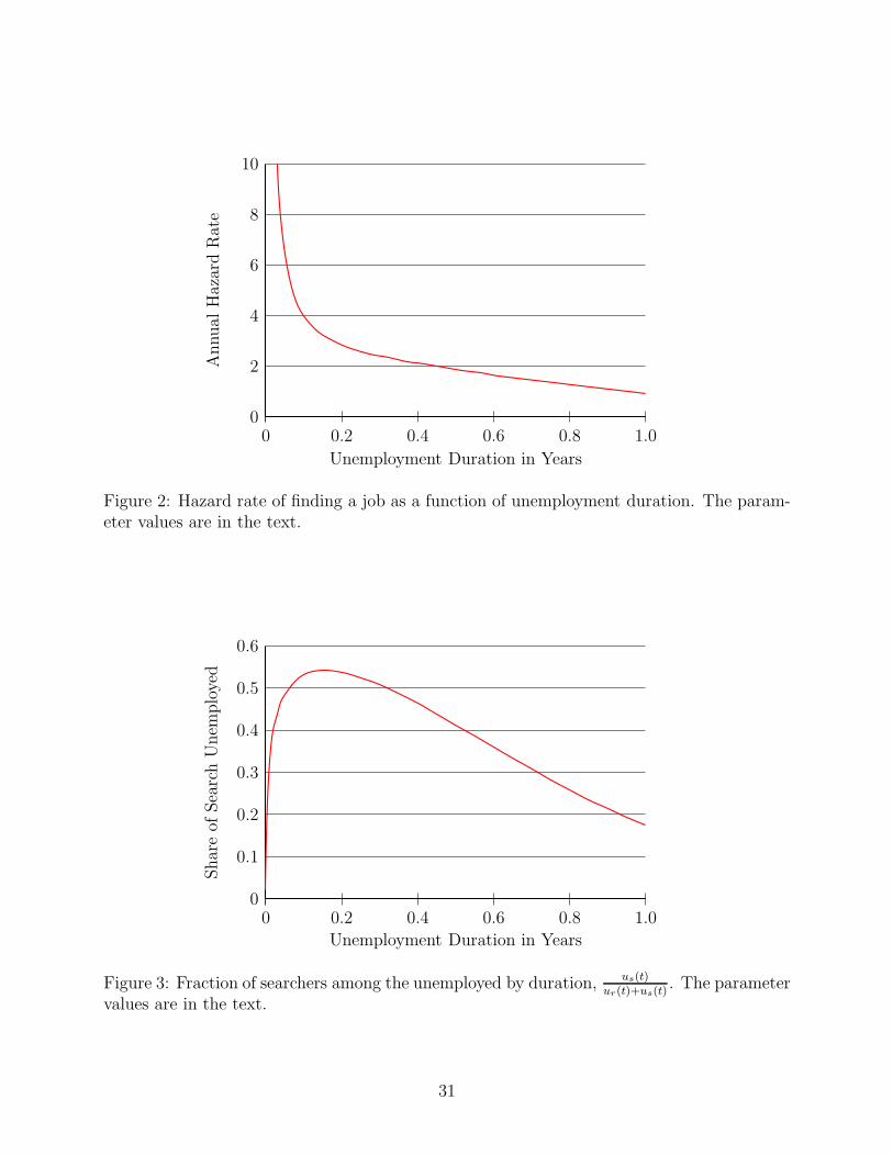
0
2
4
6
8
10
0 0.2 0.4 0.6 0.8 1.0
Unemployment Duration in Years
Annual
HazardRate
Figure 2: Hazard rate of finding a job as a function of unemployment duration. The param-eter values are in the text.
0
0.1
0.2
0.3
0.4
0.5
0.6
0 0.2 0.4 0.6 0.8 1.0
Unemployment Duration in Years
Shareof
SearchUnem
ployed
Figure 3: Fraction of searchers among the unemployed by duration, us(t)ur(t)+us(t)
. The parametervalues are in the text.
31

5 Union Objective Function
Consider a monopoly union representing the l(nj , t) workers in labor market nj at time t.
The union’s objective is to maximize the total flow utility of those workers,
e(nj, t)w(nj, t)1
C+(
l(nj , t)− e(nj, t))
br,
where e(nj, t) is the measure of workers who are employed, w(nj, t) is the wage, and 1/C is
the marginal utility of consumption. For example, we can think of the union setting the wage
and then letting competitive firms determine how many workers to hire. From the analysis
in Section 3.3, we know that employment is
e(nj , t) = min
{
l(nj , t),C(t)θn
(
Ax(nj , t))θn−1
C(n, t)θn−1wθn
}
.
The solution to the union’s problem is to set w(nj, t) = Ceω where
ω = log br + log(θn/(θn − 1)) (58)
if this leaves some workers unemployed and otherwise to set a higher level of wages consistent
with full employment, w(nj , t) = Ceω, where ω is the log full employment wage defined in
equation (33). In other words, the union sets a constant minimum wage which leaves a gap
between the utility of the members who work and those who are rest unemployed. The
minimum wage is time-invariant, although it will vary across industries depending on the
elasticity of substitution θn. This is exactly the type of policy that we have analyzed in this
paper; the analysis here simply provides a link between the minimum wage and the preference
parameters br and θn.
According to this model, the economy would be perfectly competitive in the absence of
unions. By monopolizing a labor market, a union can extract the monopoly rent. It does
this by raising wages in order to restrict employment and output and hence raise the price
of the good produced by the industry. It achieves exactly the same outcome as would be
attained by a monopoly producer facing a competitive industry.7 The model predicts that
unions will be more successful at raising wages in industries producing goods that have poor
substitution possibilities, θn close to 1.
7We do not analyze the interaction between a monopoly producer a monopoly union. In this case, settinga wage and allowing the firm to determine employment is generally inefficient. The two monopolists shouldagree on both a wage and a level of employment. Still, it seems likely that the equilibrium outcome will bea wage floor.
32

20
21
22
23
−0.1 0 0.1 0.2 0.3 0.4ω
v(ω, s)
s = 0
s = 1ω ωω
Figure 4: Value functions for s = 0, 0.1, . . . , 1. Parameters are in the text, with ω = 0.15.
Some observers have noted that, while unionization raises unemployment rates, the effects
are mitigated if unions coordinate their activities (Nickell and Layard, 1999). Our model
suggests that this may because coordinated unions are able to internalize the impact of
exploiting their monopoly power on other workers. The Pareto optimal allocation is achieved
by dropping the minimum wage constraints, so a worker can work whenever ω = log br (see
Alvarez and Shimer, 2008, Appendix B.2). Perhaps coordinated unions are able to avoid the
incentive to restrict output in individual labor markets.
6 Example
We set parameters broadly in line with those in our previous paper. Consider an industry
with an elasticity of substitution θ = 2. Let the discount rate be ρ = 0.05, the leisure value
of inactivity be bi = 1, so v = 20, and the search cost be κ = 2 so v = 22. Set the leisure
from rest unemployment to br = 0.7. Fix the standard deviation of wages at σ = 0.12 and
the quit rate at 0.04. Then let µ = q/θ − θσ2/2 ≈ 0.0056 so that we can focus on the limit
as δ → 0. Finally, set the job finding rate for searchers to α = 3.2. Since our exploration of
parameters is cursory, the results that follow should be considered preliminary.
In the absence of a minimum wage, we find that ω = −0.258, higher than log br = −0.357.
Therefore any minimum wage below this level has no effect. Figure 4 shows the value function
v(ω, s) for different seniorities when ω = 0.15. More senior workers are always better off than
less senior workers and all workers are better off when the log full employment wage ω is
higher, although more senior workers’ value function is less sensitive to ω.
Figure 5 shows how the thresholds change as functions of the minimum wage. The lower
33

0.25
0.50
0.75
1.00
−0.25
0.5 1.0−0.5ω
ω, ω
ω
ω
Figure 5: Thresholds as functions of the minimum wage ω. Parameters are in the text.
bound ω increases in ω, with a slope less than 1. Put differently, when the minimum wage
is higher, the maximum number of workers willing to stay in the industry is smaller for any
value of productivity. On the other hand, the upper bound initially falls with ω, indicating
that a modest degree of monopolization attracts workers to the industry for a given level of
productivity. This is true even though the last entrant to the union is the first worker laid
off. A monopoly union sets ω = 0.34, consistent with a ω > ω > ω.
Note that unions in our model generate not only unemployment, but also wage compres-
sion (Blau and Kahn, 1996; Bertola and Rogerson, 1997). The range of log wages is given
by the distance between the dashed 45 degree line and ω. This is declining in the minimum
wage, eventually disappearing once all workers are paid ω.
Using the computed thresholds, it is straightforward to find out how the rest and search
unemployment rates in this industry vary with ω (Figure 6). Initially there is no rest un-
employment, although search unemployment is necessary to sustain the industry. As the
minimum wage rises, the rest unemployment rate starts to increase while the search un-
employment rate is approximately unchanged. We conclude from this exercise that union-
mandated minimum wages provide a powerful mechanism for generating rest unemployment.
Figure 7 shows the annual hazard rate for two markets with different minimum wages but
the other parameters fixed at the benchmark level. In one labor market, the minimum wage is
set at ω = 0 while in the other it is at the monopoly level, ω ≈ 0.34. The overall hazard rates
are similar at short durations, roughly 1/2t, because in both cases most unemployed workers
are in rest unemployment. With a low minimum wage, few workers get trapped in long-term
unemployment because the gap between the minimum wage ω and the exit threshold ω is
34
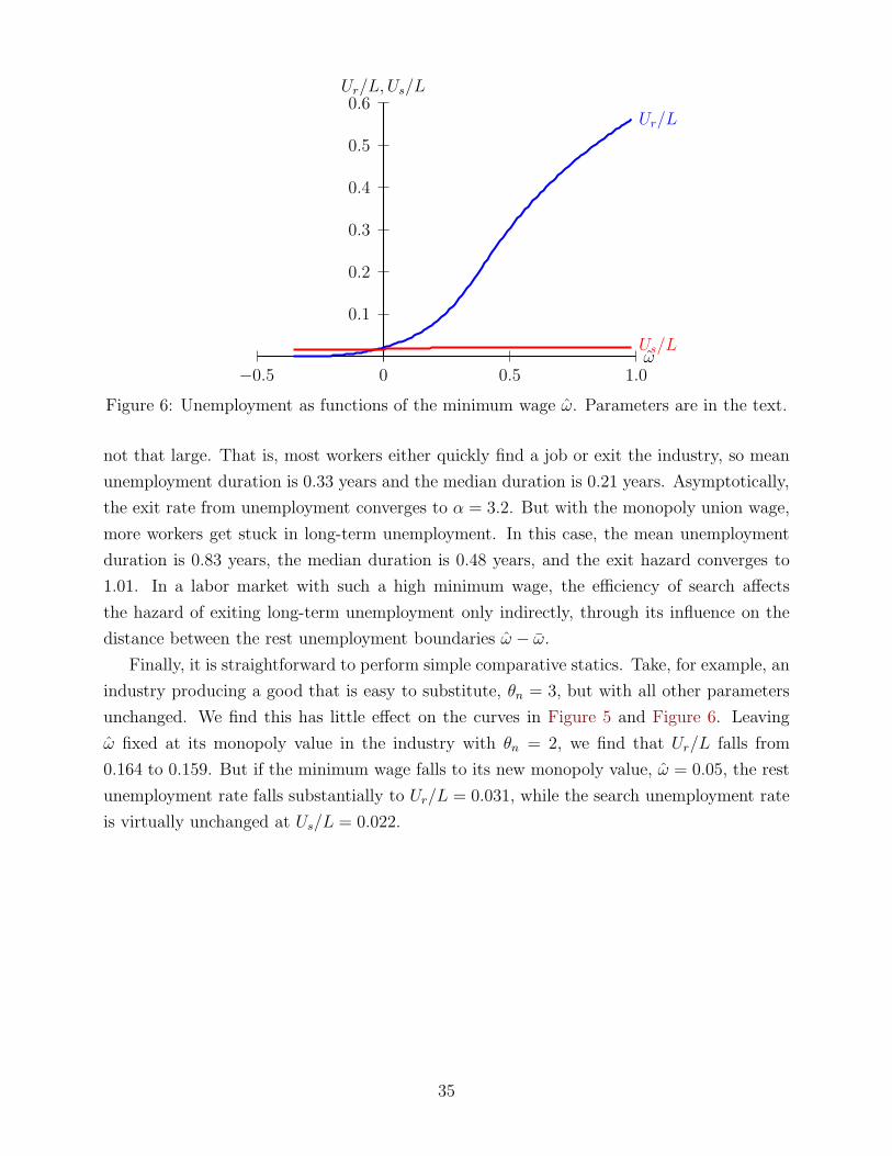
0.1
0.2
0.3
0.4
0.5
0.6
0 0.5 1.0−0.5ω
Ur/L, Us/L
Ur/L
Us/L
Figure 6: Unemployment as functions of the minimum wage ω. Parameters are in the text.
not that large. That is, most workers either quickly find a job or exit the industry, so mean
unemployment duration is 0.33 years and the median duration is 0.21 years. Asymptotically,
the exit rate from unemployment converges to α = 3.2. But with the monopoly union wage,
more workers get stuck in long-term unemployment. In this case, the mean unemployment
duration is 0.83 years, the median duration is 0.48 years, and the exit hazard converges to
1.01. In a labor market with such a high minimum wage, the efficiency of search affects
the hazard of exiting long-term unemployment only indirectly, through its influence on the
distance between the rest unemployment boundaries ω − ω.
Finally, it is straightforward to perform simple comparative statics. Take, for example, an
industry producing a good that is easy to substitute, θn = 3, but with all other parameters
unchanged. We find this has little effect on the curves in Figure 5 and Figure 6. Leaving
ω fixed at its monopoly value in the industry with θn = 2, we find that Ur/L falls from
0.164 to 0.159. But if the minimum wage falls to its new monopoly value, ω = 0.05, the rest
unemployment rate falls substantially to Ur/L = 0.031, while the search unemployment rate
is virtually unchanged at Us/L = 0.022.
35
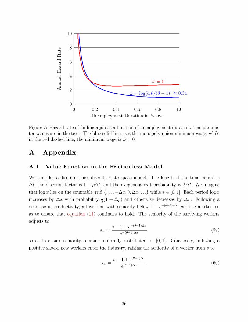
0
2
4
6
8
10
0 0.2 0.4 0.6 0.8 1.0
Unemployment Duration in Years
Annual
HazardRate
ω = log(brθ/(θ − 1)) ≈ 0.34
ω = 0
Figure 7: Hazard rate of finding a job as a function of unemployment duration. The parame-ter values are in the text. The blue solid line uses the monopoly union minimum wage, whilein the red dashed line, the minimum wage is ω = 0.
A Appendix
A.1 Value Function in the Frictionless Model
We consider a discrete time, discrete state space model. The length of the time period is
∆t, the discount factor is 1 − ρ∆t, and the exogenous exit probability is λ∆t. We imagine
that log x lies on the countable grid {. . . ,−∆x, 0,∆x, . . .} while s ∈ [0, 1]. Each period log x
increases by ∆x with probability 12(1 + ∆p) and otherwise decreases by ∆x. Following a
decrease in productivity, all workers with seniority below 1 − e−(θ−1)∆x exit the market, so
as to ensure that equation (11) continues to hold. The seniority of the surviving workers
adjusts to
s− =s− 1 + e−(θ−1)∆x
e−(θ−1)∆x, (59)
so as to ensure seniority remains uniformly distributed on [0, 1]. Conversely, following a
positive shock, new workers enter the industry, raising the seniority of a worker from s to
s+ =s− 1 + e(θ−1)∆x
e(θ−1)∆x. (60)
36

Finally, assume ∆t = (∆x/σx)2 and ∆p = µx∆x/σ
2x. This implies that log x′ is a random
walk with drift µx per unit of time:
E(log x′ − log x) = 12(1 + ∆p)∆x− 1
2(1−∆p)∆x = ∆p∆x = µx∆t.
It also has variance σ2x per unit of time, at least in the limit as ∆t→ 0:
E(log x′ − log x− µx∆t)2 = 1
2(1 + ∆p)(∆x− µx∆t)
2 + 12(1−∆p)(−∆x− µx∆t)
2
= (∆x)2 −∆p∆xµx∆t + µ2x(∆t)
2 = σ2x∆t− µ2
x(∆t)2
We thus focus on the limiting behavior as ∆t converges to 0 holding fixed µx and σx, which
corresponds to the stochastic process that we study in the body of the paper.
Now consider a worker in the discrete time, discrete state model with seniority s ≥
1− e−(θ−1)∆x, so she will remain in the market following the next shock. Her value function
satisfies
v(s) = R(s)∆t + (1− ρ∆t)(
λ∆tbi/ρ+ (1− λ∆t)(
12(1 + ∆p)v(s+) +
12(1−∆p)v(s−)
)
)
.
Consider a second order Taylor expansion of v(s+) and v(s−) around v(s):
v(s) = R(s)∆t + (1− ρ∆t)(
λ∆tbi/ρ+ (1− λ∆t)(
v(s)
+ 12(1 + ∆p)
(
v′(s)(s− 1)(e−(θ−1)∆x − 1) + 12v′′(s)(s− 1)2(e−(θ−1)∆x − 1)2
)
+ 12(1−∆p)
(
v′(s)(s− 1)(e(θ−1)∆x − 1) + 12v′′(s)(s− 1)2(e(θ−1)∆x − 1)2
)
))
.
Next approximate e−(θ−1)∆x − 1 = −(θ − 1)∆x + 12((θ − 1)∆x)2 and e−(θ−1)∆x − 1 = (θ −
1)∆x+ 12((θ− 1)∆x)2, accurate to order (∆x)2. Grouping terms and dropping any of higher
order than (∆x)2, the previous equation becomes
v(s) = R(s)∆t + (1− ρ∆t)(
λ∆tbi/ρ+ (1− λ∆t)(
v(s)
+ v′(s)(1− s)(
(θ − 1)∆p∆x− 12(θ − 1)2(∆x)2
)
+ 12v′′(s)(1− s)2(θ − 1)2(∆x)2
))
.
Now subtract (1 − ρ∆t)(1 − λ∆t)v(s) from both sides of the equation and replace ∆p =
37

µx∆x/σ2x and (∆x) = σ2
x∆t. Divide through by ∆t to get
(ρ+ λ− ρλ∆t)v(s) = R(s) + (1− ρ∆t)(
λbi/ρ
+ (1− λ∆t)(
v′(s)(1− s)(
(θ − 1)µx −12(θ − 1)2σ2
x
)
+ 12v′′(s)(1− s)2(θ − 1)2σ2
x
))
.
In particular, in the limit as ∆t→ 0, we obtain equation (13) and so this holds for all s > 0.
Now consider a worker with the lowest seniority, s = 0. Her value function satisfies
v(0) = R(0)∆t + (1− ρ∆t)(
λ∆tbi/ρ+ (1− λ∆t)(
12(1 + ∆p)v(s+) +
12(1−∆p)bi/ρ
)
)
,
since the worker will exit the market following the next shock. It is now sufficient to consider
a first order expansion of v(s+) around v(0) and to also expand e−(θ−1)∆x− 1 = −(θ− 1)∆x.
Using the value matching condition v(0) = bi/ρ, we obtain
ρ∆tv(0) = R(0)∆t + (1− ρ∆t)(1 − λ∆t)12(1 + ∆p)v′(0)(θ − 1)∆x.
This equation holds in the limit as ∆t → 0 only if v′(0) = 0 as well, the smooth pasting
condition.
A.2 Differentiability of the Value Function
Note that for ω ∈ (ω, ω), a worker’s seniority is constant; although some workers exit the
market exogenously, they are drawn uniformly from the population of workers. Now let τ(ω)
and τ(ω) denote the (stochastic) time when ω first hits ω and ω, infinite if it hits the other
boundary first. Then we can rewrite equation (42) as
v(ω0, s0; ω, ω, ω) = E
(
∫ {min{τ(ω),τ(ω)}
0
e−(ρ+λ)t(
R(ω(t), s0) + λv)
dt
+ v(ω, s0)e−(ρ+λ)τ(ω) + v(ω, s0)e
−(ρ+λ)τ(ω)
∣
∣
∣
∣
∣
ω(0) = ω0
)
.
Now let π(ω|ω0) be the discounted local time of a Brownian motion prior to the first time it
hits the boundary. Rewrite the value function as
v(ω0, s0; ω, ω, ω) =
∫ ω
ω
(
R(ω(t), s0) + λv)
π(ω|ω0)dt
+ E(
v(ω, s0)e−(ρ+λ)τ(ω) + v(ω, s0)e
−(ρ+λ)τ(ω)∣
∣ω(0) = ω0
)
.
38

Since π is everywhere continuous and is continuously differentiable except at ω0, differenti-
ating the previous expression gives
∂v(ω0, s0; ω, ω, ω)
∂ω0
=
∫ ω
ω
(
R(ω(t), s0) + λv)∂π(ω|ω0)
∂ω0
dt
+(
limω↑ω0
R(ω, s0)− limω↓ω0
R(ω, s0))
π(ω0|ω0)
+ v(ω, s0)∂Ee−(ρ+λ)τ(ω)
∂ω0+ v(ω, s0)
∂Ee−(ρ+λ)τ(ω)
∂ω0
∣
∣ω(0) = ω0.
This in turn is continuously differentiable if R(ω, s0) is continuous at ω = ω0, i.e. if s0 6=
1− eθ(ω−ω).
A.3 Discrete Time, Discrete State Space Model
We consider a discrete time, discrete state space model. The length of the time period is
∆t, the discount factor is 1 − ρ∆t, and the exogenous exit probability is λ∆t. We imagine
that ω lies on the grid {ω, ω + ∆ω, ω + 2∆ω, . . . , ω} while s ∈ [0, 1]. If at the start of the
period ω lies on the interior of the grid, it increases by ∆ω with probability 12(1 + ∆p) and
otherwise decreases by ∆ω, while s stays constant. If ω = ω, it increases to ω + ∆ω with
probability 12(1 +∆p). Otherwise, there is a negative shock. ω is unchanged and all workers
with seniority s < 1 − e−θ∆ω exit the labor market. This ensures that log employment falls
by θ∆ω, which according to equation (33) is enough to leave the log full employment wage
constant. The seniority of all other workers changes as well, falling from s to
s′ =s− 1 + e−θ∆ω
e−θ∆ω. (61)
Conversely, if ω = ω, a negative shock reduces it to ω − ∆ω with probability 12(1 − ∆p).
Otherwise there is a positive shock. ω is unchanged, but log employment rises by θ∆ω in
order to leave the log full employment wage constant. The seniority of all workers rises from
s to
s′ =s− 1 + eθ∆ω
eθ∆ω. (62)
Finally, assume ∆t = (∆ω/σ)2 and ∆p = µ∆ω/σ2. We focus on the limiting behavior as ∆ω
converges to 0 holding fixed µ and σ, which corresponds to the stochastic process that we
study in the body of the paper.
39

First take ω on the interior of the grid and an arbitrary s. The Bellman equation implies
v(ω, s) = R(ω, s)∆t+ (1− ρ∆t)(
λ∆tv
+ (1− λ∆t)(
12(1 + ∆p)v(ω +∆ω, s) + 1
2(1−∆p)v(ω −∆ω, s)
)
)
.
Take a second order Taylor expansion to v(ω ±∆ω, s) around v(ω, s) and simplify:
v(ω, s) = R(ω, s)∆t+ (1− ρ∆t)(
λ∆tv
+ (1− λ∆t)(
v(ω, s) + vω(ω, s)∆p∆ω + 12vωω(ω, s)∆ω
2)
)
.
Subtract (1 − ρ∆t)(1 − λ∆t)v(ω, s) from both sides of this equation. Since ∆p∆ω = µ∆t
and ∆ω2 = σ2∆t, we can divide through by any ∆t > 0 to obtain
(ρ+ λ− ρλ∆t)v(ω, s) = R(ω, s) + (1− ρ∆t)(
λv + (1− λ∆t)(
µvω(ω, s) +12σ2vωω(ω, s)
)
)
.
Taking the limit as ∆t→ 0 gives equation (43).
Now consider ω = ω. For s > 1− e−θ∆ω, the Bellman equation solves
v(ω, s) = R(ω, s)∆t+ (1− ρ∆t)(
λ∆tv
+ (1− λ∆t)(
12(1 + ∆p)v(ω +∆ω, s) + 1
2(1−∆p)v(ω, s′)
)
)
.
where s′ solves equation (61). Now take a first order Taylor expansion of v around (ω, s);
higher order terms would disappear from the expression. Also approximate eθ∆ω− 1 = θ∆ω.
v(ω, s) = R(ω, s)∆t+ (1− ρ∆t)(
λ∆tv
+ (1− λ∆t)(
v(ω, s) + 12(1 + ∆p)vω(ω, s)∆ω − 1
2(1−∆p)vs(ω, s)(1− s)θ∆ω
)
)
.
Subtract (1−ρ∆t)(1−λ∆t)v(ω, s) from both sides of this equation. Recall that ∆t = ∆ω2/σ2
and ∆p = µ∆ω/σ2 and divide through by ∆ω > 0:
(
ρ+ λ− ρλ∆ω
σ2
)
∆ω
σ2v(ω, s) = R(ω, s)
∆ω2
σ2+
(
1− ρ∆ω2
σ2
)
(
λ∆ω
σ2v
+
(
1− λ∆ω2
σ2
)
1
2
((
1 +µ∆ω
σ2
)
vω(ω, s)−
(
1−µ∆ω
σ2
)
vs(ω, s)(1− s)θ
)
)
.
Taking the limit as ∆ω → 0 gives equation (44). The derivation of equation (45) is almost
40

identical and hence omitted.
Now take ω = ω and s ≤ 1− e−θ∆ω. In this case, the Bellman equation solves
v(ω, s) = R(ω, s)∆t+ (1− ρ∆t)(
λ∆tv + (1− λ∆t)(
12(1 + ∆p)v(ω +∆ω, s) + 1
2(1−∆p)v
)
)
.
Taking a first order Taylor expansion of v around (ω, 0) and using v(ω, 0) = v gives
v + vs(ω, 0)s = R(ω, s)∆t+ (1− ρ∆t)(
λ∆tv
+ (1− λ∆t)(
v + 12(1 + ∆p)
(
vω(ω, 0)∆ω + vs(ω, 0)s)
))
.
Subtract (1 − ρ∆t)(1 − λ∆t)v from both sides of this equation. Recall that ∆t = ∆ω2/σ2
and ∆p = µ∆ω/σ2:
(
ρ+ λ− ρλ∆ω2
σ2
)
∆ω2
σ2v + vs(ω, 0)s = R(ω, s)
∆ω2
σ2+
(
1− ρ∆ω2
σ2
)(
λ∆ω2
σ2v
+
(
1− λ∆ω2
σ2
)
1
2
(
1 +µ∆ω
σ2
)
(
vω(ω, 0)∆ω + vs(ω, 0)s)
)
.
Taking the limit as ∆ω → 0 gives vs(ω, 0) = 0 for all s ≤ 0. Combining with equation (44)
gives equation (46).
Finally we handle the case of s = 1. Since the seniority of such a worker never changes
(see equations 61 and 62), we have
v(ω, 1) = R(ω, 1)∆t+ (1− ρ∆t)(
λ∆tv
+ (1− λ∆t)(
12(1 + ∆p)v(ω +∆ω, 1) + 1
2(1−∆p)v(ω, 1)
)
)
.
Take a first order Taylor expansion of v around (ω, 1):
v(ω, 1) = R(ω, 1)∆t+ (1− ρ∆t)(
λ∆tv + (1− λ∆t)(
v(ω, 1) + 12(1 + ∆p)vω(ω, 1)∆ω
)
)
.
Subtract (1−ρ∆t)(1−λ∆t)v(ω, 1) from both sides of this equation. Recall that ∆t = ∆ω2/σ2
and ∆p = µ∆ω/σ2 and divide through by ∆ω:
(
ρ+ λ− ρλ∆ω2
σ2
)
∆ω
σ2v(ω, 1) = R(ω, 1)
∆ω
σ2
+
(
1− ρ∆ω2
σ2
)(
λ∆ω
σ2v +
(
1− λ∆ω2
σ2
)
1
2
(
1 +µ∆ω
σ2
)
vω(ω, 1)
)
.
41
Taking the limit as ∆ω → 0 gives vω(ω, 1) = 0. A similar logic at (ω, 1) gives vω(ω, 1) = 0,
establishing equation (47).
A.4 Value Function
A.4.1 High Minimum Wage
We first tackle the case where ω ≥ ω. We claim that the value function satisfies
v(ω, s) =
eω + λv
ρ+ λ+ c1(s)e
η1(ω−ω) + c2(s)eη2(ω−ω) if s ≥ 1− eθ(ω−ω)
br + λv
ρ+ λ+ c1(s)e
η1(ω−ω) + c2(s)eη2(ω−ω) if s < 1− eθ(ω−ω),
(63)
where η1 < 0 < η2 are the roots of the characteristic equation
ρ+ λ− ηµ− η2σ2
2= 0 (64)
and the univariate functions of integration satisfy
c1(s) = −
(
η2η2 − η1
)(
eω − brρ+ λ
)
(1− e−(η2−η1)(ω−ω))(1− s)−η1/θ (65)
c2(s) = 0 (66)
c1(s) = c1(s) +
(
η2η2 − η1
)(
eω − brρ+ λ
)
(1− s)−η1/θ (67)
c2(s) = c2(s) +
(
−η1η2 − η1
)(
eω − brρ+ λ
)
(1− s)−η2/θ, (68)
where we leave the expressions in a convenient form.
To prove this, note first that equation (63) is the general solution to equation (43).
All that remains is to characterize the four functions of integration. The condition that
the value function is continuously differentiable even at the boundary between work and
rest unemployment, i.e. points of the form (ω, 1 − eθ(ω−ω)), yields equations (67) and (68).
Equations (44) and (45) then reduce to ci(s)ηi = c′i(s)(1 − θ)s for i = 1, 2, or equivalently
ci(s) = ci(1− s)−ηi/θ.
To pin down the two constants c1 and c2, we use two more boundary conditions. Differ-
entiate equation (63) to get
vω(ω, s) = c1(1− s)−η1/θη1eη1(ω−ω) + c2(1− s)−η2/θη2e
η2(ω−ω)
42

when s ≥ 1 − eθ(ω−ω). In particular, equation (47) implies that this should converge to 0
as s → 1 at ω = ω or ω = ω. Since η2 > 0 > η1, this implies c2 = 0, which delivers
equation (66). Note that this implies vω(ω, 1) = 0 for all ω, since a worker at s = 1 will earn
ω regardless of the subsequent sequence of shocks. Finally, use equation (46) to pin down
the last constant c1, yielding equation (65).
A.4.2 Moderate Minimum Wage
Next we turn to the case where ω > ω ≥ ω. The basic approach is similar. We claim that
the value function satisfies
v(ω, s) =
eω
ρ+ λ− µ− 12σ2
+λv
ρ+ λ+ c1(s)e
η1(ω−ω) + c2(s)eη2(ω−ω) if ω ≥ ω
eω + λv
ρ+ λ+ c1(s)e
η1(ω−ω) + c2(s)eη2(ω−ω) if ω < ω and s ≥ 1− eθ(ω−ω)
br + λv
ρ+ λ+ c1(s)e
η1(ω−ω) + c2(s)eη2(ω−ω) if ω < ω and s < 1− eθ(ω−ω),
(69)
where η1 < η2 solve equation (64) and
c1(s) = e−η1ωc1(1− s)−η1/θ − e−η1ω(
eω
ρ+ λ
)(
ρ+ λ− (µ+ 12σ2)η2
(ρ+ λ− µ− 12σ2)(η2 − η1)
)
(70)
+ e−η1ωeω(
e−(ω−ω)(η2−η1)(1−e−(ω−ω)(η2−1))−η1
+(1−e−(ω−ω)(η2−η1))(ρ+λ−(µ+ 1
2σ2)η2)
(ρ+λ)(η2−η1)
)
(1− e−(ω−ω)(η2−η1))(ρ+ λ− µ− 12σ2)
(71)
(72)
c2(s) = e−η2ωc2(1− s)−η2/θ + e−η2ω(
eω
ρ+ λ
)(
ρ+ λ− (µ+ 12σ2)η1
(ρ+ λ− µ− 12σ2)(η2 − η1)
)
(73)
− e−η2ωeω(
e(ω−ω)(η2−η1)(1−e(ω−ω)(1−η1))η2
+(1−e(ω−ω)(η2−η1))(ρ+λ−(µ+ 1
2σ2)η1)
(ρ+λ)(η2−η1)
)
(1− e(ω−ω)(η2−η1))(ρ+ λ− µ− 12σ2)
where (74)
c1 = −
(
η2η2 − η1
)(
eω
ρ+ λ
)
(
1− e−(ω−ω)(η2−η1))
and c2 = 0 .
For ω ≥ ω:
a1 = e−η1ω(
eω
ρ+ λ
)(
ρ+ λ− (µ+ 12σ2)η2
(ρ+ λ− µ− 12σ2)(η2 − η1)
)
(75)
a2 = −e−η2ω(
eω
ρ+ λ
)(
ρ+ λ− (µ+ 12σ2)η1
(ρ+ λ− µ− 12σ2)(η2 − η1)
)
(76)
43

If ω < ω and s < 1− eθ(ω−ω):
h1(s) = e−η1ω(
η2η2 − η1
)(
eω
ρ+ λ
)
(1− s)−η1/θ (77)
h2(s) = −e−η2ω(
η1η2 − η1
)(
eω
ρ+ λ
)
(1− s)−η2/θ. (78)
Once again, equation (69) is the general solution to equation (43). Continuity and dif-
ferentiability of the value function again allow us to relate ci(s) to ci(s) and ci(s) to ci(s).
Then equations (44) and (45) yield a pair of differential equations which can be solved for
c1(s) and c2(s) as a function of parameters and the two constants c1 and c2. This gives
equations (??)–(77). Equation (47), evaluated either at ω or ω, again pins down c2 = 0 so
that c2(s) remains finite as s→ 1. Finally, use equation (46) to pin down c1.
Proposition 6. Let ω ≥ ω ≥ ω with at least one of the inequalities strict. Then there is
a unique function v (ω, s) that satisfies: i) the BJH equation
ρv (ω, s) = R (ω, s) + µvω (ω, s) + vωω (ω, s)σ2
2
at all (ω, s) except those on {(ω, s) : ω ≤ ω ≤ ω, s = − exp (−θ (ω − ω))} , ii) The boundary
conditions vω (ω, s) = θ (1− s) vω (ω, s) hold at ω ∈ {ω, ω} and s ∈ [0, 1), iii) The smooth
pasting condition vω (ω, s) = 0 hold at (ω, s) ∈ {(ω, 0) , (ω, 1) , (ω, 1)} , iv) The function v is
C2 on [ω, ω]× [0, 1), except at
(ω, s) ∈ {(ω, s) : ω ≤ ω ≤ ω, s = − exp (−θ (ω − ω))}
where it is C1. v) The function v (·, 1) is C2 on [ω, ω] . Moreover, v (ω, s) is given by
v (ω, s) =eω
ρ− µ− σ2/2+∑
i=1,2
[ci (s) + ai] eηiω
for ω ∈ [ω, ω] ,
v (ω, s) =∑
i=1,2
[ci (s) + hi (z (s))] eηiω
for ω ∈ [ω, ω] and s ≤ 1− exp (−θ (ω − ω)) and
v (ω, s) =eω
ρ+∑
i=1,2
ci (s) eηiω
for ω ∈ [ω, ω] and s ≥ 1 − exp (θ (ω − ω)) . The functions ci (s) : [0, 1] → R, and hi :
44

[0, θ (ω − ω)] → R, and the numbers ai are as follows. Let the matrices M and N be
M ≡
[
eη1ω eη2ω
η1eη1ω η2e
η2ω
]
,
N ≡
[
eη1ωη1 eη2ωη2
eη1ωη1 eη2ωη2
]
Then the constants ai are given by
a =M−1 eω
[
1ρ− 1
ρ−µ−σ2/2
− 1ρ−µ−σ2/2
]
.
Let the function z : [0, 1] → R be
z (s) ≡ − log (1− s) .
Then the functions hi (·) are given by
hi (z (s)) = hi (0) eηiθz(s)
for all s ∈ [0, 1] with
h (0) =M−1
[
eω
ρ
0
]
,
The functions ci (·) are given by
c2 (s) = c2 (1)
for i = 2 for all s ∈ [0, 1] . For i = 1
c1 (s) = [c1 (0)− c1 (1)] eη1z(s) + c1 (1)
for all s ∈ [0, 1] . Finally, c1 (0) given by
c1 (0) =−eη2ωη2 c2 (1)−
∑
i=1,2 hi (0) eηiωηi
eη1ωη1
and the vector c (s) evaluated at s = 1 is given by:
c (1) = N−1
[
−g
0
]
45

where the number g is given by
g ≡eω
ρ− µ− σ2/2+∑
i=1,2
aieηiωηi .
Proof. Let σi (z (s)) ≡ ci (s) or σi (·) ≡ ci (z−1 (·)) . Notice that
(1− s) c′i (s) = σ′i (z (s))
where ci stands for ci, ci or ci and likewise for σi. We use c (s) = c (s)+ai, ci (s) = ci (s)+hi (s)
Given that η1 < 0 < η2 and ω > ω the matrices M and N are invertible since
detM = e(η1+η2)ω (η2 − η1) 6= 0
detN = (η1η2)(
eη1ω+η2ω − eη2ω+η1ω)
6= 0
Proof. (of Proposition 6) Step I. Solve for σi (z) as a function of σi (z) for all z.
Write the equations for value matching and smooth pasting between regions 1 and 2 for
all z ∈ (0,∞) as:
eω
ρ− µ− σ2/2+∑
i=1,2
σi (z) eηi ω =
eω
ρ+∑
i=1,2
σi (z) eηi ω
eω
ρ− µ− σ2/2+∑
i=1,2
σi (z) ηieηi ω =
∑
i=1,2
σi (z) ηi eηi ω
Using these two equations we can solve for σ (z) as a function of σ (z) . The solution gives:
σi (z) = σi (z) + ai
for two constants a1, and a2. This can be seen by replacing into the equations above and
obtaining:
eω
ρ− µ− σ2/2+∑
i=1,2
ai eηi ω =
eω
ρ
eω
ρ− µ− σ2/2+∑
i=1,2
ai ηieηi ω = 0
46

or
a = eω M−1
[
1ρ− 1
ρ−µ−σ2/2
− 1ρ−µ−σ2/2
]
Step II. Solving σ (∞) = ci (1) and σi (∞) = ci (1) .
We have that at s = 1, vω (ω, 1) = 0 at ω ∈ {ω, ω} so that
∑
i=1,2
σi (∞) eηiωηi = −eω
ρ− µ− σ2/2∑
i=1,2
σi (∞) eηiωηi = 0
Together with σi (z) = σi (z) + ai this implies:
∑
i=1,2
σi (∞) eηiωηi = −g (ω, ω)
∑
i=1,2
σi (∞) eηiωηi = 0
where
g ≡eω
ρ− µ− σ2/2+∑
i=1,2
ai (ω) eηiωηi
The solution of this system gives σi (∞) or
c (1) ≡ σ (∞) = N−1
[
−g
0
]
Step III. Solve ode’s for σi (z) for z ≥ θ (ω − ω)
Consider the ode’s for σ and σ for s ≥ s = 1− exp (−θ (ω − ω)) or
z ≥ θ (ω − ω)
They are given by vω = (1− s) θvs evaluated at ω ∈ {ω, ω} or
eω
ρ− µ− σ2/2+∑
i=1,2
σi (z) ηieηi ω = θ
∑
i=1,2
σ′i (z) e
ηi ω
∑
i=1,2
σi (z) ηieηi ω = θ
∑
i=1,2
σi (z) eηi ω
47

Using the result for σ in terms of σ :
σ′i (z) = σ′
i (z)
or
eω
ρ− µ− σ2/2+∑
i=1,2
aiηieηi ω +
∑
i=1,2
σi (z) ηieηi ω = θ
∑
i=1,2
σ′i (z) e
ηi ω
∑
i=1,2
σi (z) ηieηi ω = θ
∑
i=1,2
σ′i (z) e
ηi ω
The solution of this system is given by
σi (z) = eηiθz fi + di
where di solve
g +∑
i=1,2
di ηieηi ω = 0
∑
i=1,2
di ηieηi ω = 0
for g defined as above, thus
d = N−1
[
−g
0
]
or, by comparing both systems
d = c (1) .
Step IV Solve for σ(z) as functions of σ (z) for z ≤ θ (ω − ω)
For z ∈ (0, z) we have two other value matching and smooth pasting between regions 2
and 3:
∑
i=1,2
σi (z) eηi ω(z) =
eω
ρ+∑
i=1,2
σi (z) eηi ω(z)
∑
i=1,2
σi (z) ηieηi ω(z) =
∑
i=1,2
σi (z) ηi eηi ω(z)
48

where ω (z) is given by
ω (z) = ω −1
θz ⇐⇒ s = 1− exp (−θ (ω − ω))
so we have
∑
i=1,2
σi (z) e−
ηiθzeηi ω =
eω
ρ+∑
i=1,2
σi (z) e−
ηiθzeηi ω
∑
i=1,2
σi (z) ηie−
ηiθzeηi ω =
∑
i=1,2
σi (z) ηie−
ηiθz eηi ω
These equations imply that
σi (z) = σi (z) + hi (z)
where hi (z) satisfy
∑
i=1,2
hi (z) e−
ηiθzeηi ω =
eω
ρ∑
i=1,2
hi (z) ηie−
ηiθzeηi ω = 0
for all z ∈ (0, z) .We try the solution
hi (z) = hi (0; ω) eηiθz
h (0) = M−1
[
eω
ρ
0
]
For future reference notice that h′i (z) = (ηi/θ)hi (z) .
Step V. Solve ode’s for σ in z ∈ (0, θ (ω − ω))
In this region we also have two boundary conditions, corresponding to vω = vsθ (1− s) evaluated
at ω ∈ {ω, ω} . This gives the ode’s:
eω
ρ− µ− σ2/2+∑
i=1,2
σi (z) eηiωηi = θ
∑
i=1,2
σ′i (z) e
ηiω
and∑
i=1,2
σi (z) eηiωηi = θ
∑
i=1,2
σ′i (z) e
ηiω
49
replacing that
σi (z) = σi (z) + ai
σi (z) = σi (z) + hi (z)
we have:
eω
ρ− µ− σ2/2+∑
i=1,2
aieηiωηi +
∑
i=1,2
σi (z) eηiωηi
= θ∑
i=1,2
σ′i (z) e
ηiω
and
−θ∑
i=1,2i
h′i (z) eηiω +
∑
i=1,2
hi (z) eηiωηi +
∑
i=1,2
σi (z) eηiωηi
= θ∑
i=1,2
σ′i (z) e
ηiω
or using that h′i (z) = (ηi/θ) hi (z)
∑
i=1,2
σi (z) eηiωηi = θ
∑
i=1,2
σ′i (z) e
ηiω
for z ∈ (0, z) . We can also write this system as:
g +∑
i=1,2
σi (z) eηiωηi = θ
∑
i=1,2
σ′i (z) e
ηiω
∑
i=1,2
σi (z) eηiωηi = θ
∑
i=1,2
σ′i (z) e
ηiω
where g is defined as above.
This system of linear odes is the same as the one that applies for z ≥ θ (ω − ω) . Since
we require σi (z) to be continuously differentiable at z = z, the solution must also be given
σi (z) = eηiθzfi + di for the same constants f, d in the entire domain z ≥ 0. Since we have
shown that d = c (1) , we can write:
σi (z) = eηiθzfi + ci (1)
= eηiθz (σi (0)− ci (1)) + ci (1)
50

for z ≥ 0.
Step VI. Using the unstable root to determine one initial condition for σi.
From the previous step we have that
σi (z) = eηiθzfi + ci (1)
Recall that η1 < 0 < η2, and that at s = 1, or equivalently z → ∞
ci (1) ≡ limz→∞
σi (z)
ci (1) ≡ limz→∞
σi (z)
we have finite values. Thus the coefficient f2 associated with the unstable root η2 > 0 must
be zero so that for all z ≥ 0 :
σ2 (z) = c2 (1) , σ2 (z) = c2 (1) + a2
and thus
σ2 (z) = c2 (1) + h2 (0) eη2θz
for z ∈ [0, z] .
Step VII. Using vω (ω, 0) = 0 to determine an initial condition for σi (0)
Finally at (ω, s) = (ω, 0) we have vω = 0 or
∑
i
σi (0) eηiωηi = 0
or using σi (z) = σi (z) + hi (z) at z = 0 :
∑
i=1,2
σi (0) eηiωηi = −
∑
i=1,2
hi (0) eηiωηi
This gives one equation for {σi (0)}i=1,2 .
Step VIII. Solve for σ (0) .
From step VI we have
σ2 (0) = c2 (1) ,
and using step VII∑
i=1,2
σi (0) eηiωηi = −
∑
i=1,2
hi (0) eηiωηi
51

or
σ1 (0) =−eη2ωη2 c2 (1)−
∑
i=1,2 hi (0) eηiωηi
eη1ωη1
QED.
A.4.3 Low Minimum Wage
Finally we study ω < ω. This is equivalent to the case when ω = ω, since in both situations
the minimum wage never binds. Applying the analysis with a moderate minimum wage gives
v(ω, s) =eω
ρ+ λ− µ− 12σ2
+λv
ρ+ λ+ c1e
η1(ω−ω) + c2eη2(ω−ω) (79)
where η1 < η2 solve equation (64) and
c1 =eω(
1− e−(ω−ω)(η2−1))
−η1(1− e−(ω−ω)(η2−η1))(ρ+ λ− µ− 12σ2)
(80)
c2 = −eω(
1− e(ω−ω)(1−η1)))
η2(1− e(ω−ω)(η2−η1))(ρ+ λ− µ− 12σ2)
. (81)
Note that the value function does not depend on the worker’s seniority.
A.5 Existence of Equilibrium for the λ = 0 case
We let ηi be the roots of
0 = ρ− ηµ− ησ2/2
and assume that ρ > µ+ σ2/2 so we have η1 < 0 < 1 < η2.
Proposition 7. Monotonicity of v, given thresholds. Let v (ω, s) be defined above for
given tripe ω≤ ω ≤ω. Then:
i) The derivative vs (ω, s) > 0 for all s < 1, except at (ω, s) = (ω, 0) .
ii) The derivative vω (ω, s) > 0 everywhere expect at (ω, s) ∈ {(ω, 0) , (ω, 1) , (ω, 1)} .
Proof. First recall that in our previous paper we show that v (ω, 1) is strictly increasing in
ω ∈ (ω, ω). Since this function satisfies: vω (ω, 1) = 0, it implies that vωω (ω, 1) > 0, which
in turns implies that:
c1 (1) > 0 and c2 (2) > 0.
52

This follows because 0 < η1 < η2
vω (ω, 1) =∑
i=1,2
ci (1) eηiωηi = 0, and
vωω (ω, 1) =∑
i=1,2
ci (1) eηiω (ηi)
2 > 0.
Monotonicity of v (ω, s) w.r.t. to s.
For future reference we notice that in region 3 (i.e. ω ≤ ω and s ≤ 1−exp (−θ (ω − ω))) we
have:
vs (ω, s) =1
1− s[σ′
1 (z (s)) eη1ω + σ′
2 (z (s)) eη2ω]
=1
1− s[(σ′
1 (z) + h′1 (z (s))) eη1ω + h′2 (z (s)) e
η2ω]
=1
1− s
[η1θ[σ1 (z (s))− c1 (1) + h1 (z)] e
η1ω +η2θh2 (z (s)) e
η2ω]
=1
1− s
[η1θ[σ1 (0)− c1 (1) + h1 (0)] e
η1θz(s)eη1ω +
η2θh2 (0) e
η2θz(s)eη2ω
]
Since by construction we have vs (ω, 0) = 0, this implies:
−η1 [σ1 (0)− c1 (1)] = η1h1 (0) eη1ω + η2h2 (0) e
η2ω
From the two equations that define h (0) , using that η1 < 0 < η2 ,we have
h1 (0) > 0 and h2 (0) > 0.
Moreover, let H (ω) be
H (ω) ≡ η1h1 (0) eη1ω + η2h2 (0) e
η2ω
so that
Hω (ω) = (η1)2 h1 (0) e
η1ω + (η2)2 h2 (0) e
η2ω > 0
By definition of h (0) we have H (ω) = 0, then we can write the previous equation as
(−η1) [σ1 (0)− c1 (1)] = H (ω) < H (ω) = 0.
Now we use this inequality to show that in region 2 (i.e. ω ≤ ω and z ≥ θ (ω − ω)) the
function v (ω, s) is increasing in s :
vs (ω, s) =1
1− sσ′1 (z (s)) e
η1ω =1
1− s
η1θe
η1θz(s) (σ1 (0)− c1 (0)) e
η1ω ≥ 0
53

Moreover in region 1 (i.e., ω ≥ ω) we have
vs (ω, s) =1
1− sσ′1 (z (s)) e
η1ω =1
1− sσ′1 (z (s)) e
η1ω
so that v is also increasing in s. For region 3 notice that we can write the previous expression
as
(1− s) vs (ω, s) = J (ω, z)
where
J (ω, z) ≡η1θ[σ1 (0)− c1 (1) + h1 (0)] e
η1θzeη1ω +
η2θh2 (0) e
η2θzeη2ω
Since c2 (1) > 0, h2 (0) > 0, η1 < 0 < η2, and
0 = vω (ω, 0) = η1 [σ1 (0)− c1 (1) + h1 (0)] eη1ω + η2 [c2 (1) + h2 (0)] e
η2ω
we have σ1 (0) = σ1 (0)− c1 (1) + h1 (0) > 0. Moreover using these inequalities we obtain:
Jω (ω, z) =(η1)
2
θ[σ1 (0)− c1 (1) + h1 (0)] e
η1θzeη1ω +
(η2)2
θh2 (0) e
η2θzeη2ω > 0
Jz (ω, z) = (η1/θ)2 [σ1 (0)− c1 (1) + h1 (0)] e
η1θzeη1ω + (η2/θ)
2 h2 (0) eη2θzeη2ω > 0
Thus for ω >ω and z > 0 we have J (ω, z) > 0 since J (ω, 0) = 0, and hence vs (ω, s) > 0 in
region 3.
Monotonicity w.r.t. ω.
In region 1 (i.e. ω ≥ ω) we have the following:
vω (ω, s) =eω
ρ− µ− σ2/2+∑
i=1
σi (z (s)) ηieηiω
and in particular for s = 1
vω (ω, 1) =eω
ρ− µ− σ2/2+∑
i=1
ci (1) ηieηiω > 0
for all ω ∈ (ω, ω) , from the result in our previous paper. We have that σ1 (z) = σ1 (z)+a1 and
σ2 (z) = c2 (1) + a2 so
vωs (ω, s) =1
1− sη1σ
′1 (z (s)) e
η1ω =1
1− s(η1)
2 [σ1 (0)− c1 (1)] eη1θz(s)eη1ω < 0
since we have shown that σ1 (0) − c1 (1) < 0. Thus vω (w, s) > vω (w, 1) > 0 for all 0 ≤ s <
54
1 and ω ≥ ω.
In region 2 we have, from our previous paper,
vω (ω, 1) =∑
i=1
ci (1) ηieηiω > 0
and as in region 1:
vωs (ω, s) =1
1− sη1σ
′1 (z (s)) e
η1ω =1
1− s(η1)
2 [σ1 (0)− c1 (1)] eη1θz(s)eη1ω < 0
so vω (w, s) > vω (w, 1) > 0 for ω ≤ ω and z ≥ θ (ω − ω) .
In region 3, ω ≤ ω, and z ≤ θ (ω − ω) we have
vω (ω, s) = θ (1− s) vs (ω, s) > 0
for all s > 0, where the equality follows by construction, and the strict inequality has been
shown above.
We have shown above that σi (0) = [σi (0) + hi (0)] > 0 for i = 1, 2. By construction we
have vω (ω, 0) = 0, and
vωω (ω, 0) =∑
i=1,2
σi (0) (ηi)2 eηiω > 0
Thus for all ω< ω ≤ ω,
vω (ω, 0) > vω (ω, 0) = 0
Also we have
(1− s) vωs (ω, s)
= η1 [σ (z (s)) + h′1 (z (s))] eη1ω + η2h
′2 (z (s)) e
η2ω
=(η1)
2
θe
η1θz(s) [σ1 (0)− c1 (0) + h1 (0)] e
η1ω
+(η2)
2
θh2 (0) e
η2θz(s) eη2ω
> 0
and thus
vω (ω, s) > vω (ω, 0) > 0
in the interior of region 3. QED.
55

We let v (ω, s;ω, ω, ω) be the value function of an agent with state (ω, s) when the economy
is characterized by thresholds {ω, ω} and minimum wage ω.
Proposition 8. Equilibrium lower bound. Let ∗v = v (ω, 0; ω, ω, ω) . Let ω ≥ ω and
0 ≤ v ≤ ∗v. There is a unique ω = Γ (v; ω, ω) ≤ ω that solves
v (ω, 0;ω, ω, ω) = v .
The function Γ is increasing in v and decreasing in ω. Moreover, if ω = ω
Γ (v; ω, ω) → (1/η2) log
v
h2 (0)[
1− η2η1
]
= ω (1− η2) +1
η2log (ρ v)
and that
limω→∞
Γ (v; ω, ω) → (1/η2) log
v
[h2 (0)− a2][
1− η2η1
]
which is finite.
Proof. To conserve notation let ξ defined as
v (ω, 0;ω, ω, ω) ≡ ξ (ω) = [c2 (1) + h2 (0)] eη2ω
[
1−η2η1
]
where we notice that c2 (1) depends on ω. We want to show that
∂
∂ωξ (ω) = eη2ω
[
1−η2η1
](
[c2 (1) + h2 (0)] η2 +∂
∂ωc2 (1)
)
> eη2ω[
1−η2η1
]
[c2 (1) + h2 (0)] η2 > 0
We have established that c2 (1)+ h2 (0) > 0 and since η1 < 0 < η2 it will suffice to show that
c2 (1) is an increasing function of ω. That c2 is increasing in ω, and that c2 (1) + h2 (0) >
0, implies that as ω→ −∞, then ξ → 0. The vector c (1;ω) solves:
∑
i=1,2
ci (1) eηiωηi = −g
∑
i=1,2
ci (1) eηiωηi = 0
56

where g is not a function of ω. This system gives
c2 (1) =e−η1ωg
η2 [e(η2−η1)ω − e(η2−η1)ω].
If ω = ω, then g = 0 and c2 (1) = 0 for all ω. This follows because in this case g is given
by:
g ≡eω
ρ− µ− σ2/2+∑
i=1,2
aieηiωηi
and ai satisfies
eω
ρ− µ− σ2/2+∑
i=1,2
ai eηi ωηi = 0.
Moreover, we have that h (0) solves:
∑
i=1,2
hi (0) eηi ω =
eω
ρ∑
i=1,2
hi (0) eηi ωηi = 0
or
eη1ωh1 (0) =eω
ρ− eη2ωh2 (0)
eη1ωh1 (0) = −eη2ωh2 (0)η2η1
thus
h2 (0) =eω/ρ
eη2ω(
1− η2η1
) > 0,
h1 (0) = −η2η1
eω/ρ
eη1ω(
1− η2η1
) > 0
Replacing h2 (0) into the expression for ω:
ω =1
η2log
v
h2 (0)[
1− η2η1
]
= ω (1− η2) +1
η2log (ρ v)
57

When ω → ∞ we have
c2 (1) =e−η2ωg
η2 [e(η2−η1)(ω−ω) − 1]
e−η2ωg =e(1−η2)ω
ρ− µ− σ2/2+∑
i=1,2
aie(ηi−η2)ωηi
=e(1−η2)ω
ρ− µ− σ2/2+ a1e
(η1−η2)ωη1 + a2η2
and
η2 =−µ+
√
µ2 + 2σ2ρ
σ2>
−µ+√
µ2 + 2σ2 (µ+ σ2/2)
σ2
=−µ+
√
µ2 + 2σ2µ+ σ2
σ2=
−µ+ µ+ σ2
σ2= 1
so that
1− η2 < 0
and thus
limω→∞
c2 (1) =limω→∞ e−η2ωg
−η2=η2a2−η2
= −a2
Also h2 (0)− a2 > 0 since by defintion h (0)− a satisfy
[h (0)− a] =M−1 eω
[
1ρ−µ−σ2/2
1ρ−µ−σ2/2
]
and it is easy to verify that h2 (0)−a2 < 0 leads to a contradiction (from the first equation if
h2 (0)− a2 (0) < 0, then it must be that h1 (0)− a1 > 0. But then arrive to a contradiction
from the second equation, since η1 < 0 < η2).
∂
∂ωc2 (1) = c2 (1)
(η2 − η1)
[e(η2−η1)ω − e(η2−η1)ω]≥ 0
Thus,
∂
∂ωξ (ω) = eη2ω
[
1−η2η1
](
[c2 (1) + h2 (0)] η2 + c2 (1;ω)(η2 − η1)
[e(η2−η1)ω − e(η2−η1)ω]
)
> 0
58

Notice that
limω→∞
ξ (ω) = 0
ξ (ω) = ∗v (ω, ω)
To see why notice that when ω =ω the minimum wage does not bind and indeed we have:
v (ω, s; ω, ω, ω) = v (ω, 0; ω, ω, ω)
for all s. To see why notice that
v (ω, 1; ω, ω, ω) =eω
ρ− µ− σ2/2+∑
i=1,2
[ci (1) + ai] eηiω
v (ω, 0; ω, ω, ω) =eω
ρ+∑
i=1,2
[ci (1) + hi (0)] eηiω
We also have that v (ω, 1; ω, ω, ω) can be written as
v (ω, 1; ω, ω, ω) =eω
ρ− µ− σ2/2+∑
i=1,2
[ci (1) + ai] eηiω
where vω (ω, 1; ω, ω, ω) = vω (ω, 1; ω, ω, ω) = 0, or ci (1) + ai solve:
∑
i=1,2
[ci (1) + ai] eηiωηi = −
eω
ρ− µ− σ2/2
∑
i=1,2
[ci (1) + ai] eηiωηi = −
eω
ρ− µ− σ2/2
Clearly these are implied by our system when ω =ω:
eω
ρ− µ− σ2/2+∑
i=1,2
ai eηi ω =
eω
ρ
eω
ρ− µ− σ2/2+∑
i=1,2
ai ηieηi ω = 0
59

∑
i=1,2
ci (1) eηiωηi = −
eω
ρ− µ− σ2/2−∑
i=1,2
aieηiωηi
∑
i=1,2
ci (1) eηiωηi = 0
∑
i=1,2
hi (0) eηi ω =
eω
ρ∑
i=1,2
hi (0) ηieηi ω = 0
Given that ξ is continuous and ranges from 0 to ∗v (ω, ω) the existence of Γ follows from
the intermediate value theorem, and its uniqueness from the fact that ξ is strictly increasing.
Finally we show Γ is decreasing in ω. Recognizing the dependence of ci (1) on ω, we first
show that c2 (1) is increasing in ω. We do so using some results from our previous papers.
We have that for s = 1 and ω ≥ ω
v (ω, 1;ω, ω, ω) =eω
ρ− µ− σ2/2+∑
i=1,2
[ci (1) + ai] eηiω
and for ω < ω :
v (ω, 1;ω, ω, ω) =eω
ρ+∑
i=1,2
ci (1) eηiω
We have that vω (ω, 1;ω, ω, ω) = vω (ω, 1;ω, ω, ω) = 0. Then
vω (ω, 1;ω, ω, ω) =∑
i=1,2
∂
∂ωci (1) e
ηiω > 0
and likewise:
vω (ω, 1;ω, ω, ω) =∑
i=1,2
∂
∂ωci (1) e
ηiω > 0
where the inequalities follow using the result in our previous paper. This implies that at
least one of the derivatives ∂∂ωci (1) must be positive. Suppose, by way of contradiction, that
∂∂ωc2 (1) < 0 and thus ∂
∂ωc1 (1) > 0. From the formula in our previous paper we also have that
vω (ω, 1;ω, ω, ω) > vω (ω, 1;ω, ω, ω)
60

Thus:∂
∂ωc1 (1) [e
η1ω − eη1ω] +∂
∂ωc2 (1) [e
η2ω − eη2ω] > 0
a contradiction since η1 < 0 < η2 and ω >ω.
Thus c2 (1) is increasing in ω, ξ (ω) shifts up with as ω increases, and hence Γ(v; ω, ω) is
decreasing in ω.
QED.
Proposition 9. Critical values for minimum wage. (i) Let ω∗ be the value of ω such that
there is a ω = ω∗ such that
v (ω∗, 0;ω∗, ω∗, ω∗) = v,
v (ω∗, 0;ω∗, ω∗, ω∗) = v .
Hence at ω = ω∗ the minimum wage is so high that region 1 is about to disappear, i.e.
ω = ω = ω∗. There exists a unique value of ω∗ that satisfy these equations and is given by a
decreasing function γ∗ :
ω∗ = log (v) + γ∗
(
v
v
)
.
(ii) Let ∗ω be the value of ω such that there is ω = ∗ω for which
v (∗ω, 0;∗ ω,∗ ω,∗ ω) = v,
v (∗ω, 0;∗ ω,∗ ω,∗ ω) = v .
Hence at ω = ∗ω the minimum wage is just high enough so that it binds, i.e. ω = ω = ∗ω.
(iii) The threshold values satisfy ∗ω < ω∗.
Proof. (i) When ω = ω we have that ω∗ must solve
v = v (ω∗, 0;ω∗, ω∗, ω∗) =eω
ρ+ c2 (1) e
η2ω
[
1− e(η1−η2)(ω−ω)η2η1
]
−eη1(ω−ω)
η1
[
∑
i=1,2
hi (0; ω) eηiωηi
]
sinceeω
ρ− µ− σ2/2+∑
i=1,2
ai eηi ω =
eω
ρ.
61

Moreover, with ω = ω we have c2 (1) = c1 (1) = 0, since g (ω, ω) = 0, and thus:
v =eω
ρ−eη1(ω−ω)
η1
[
∑
i=1,2
hi (0; ω) eηiωηi
]
=eω
ρ− eη1ω
[
h1 (0) + h2 (0) e(η2−η1)ω
η2η1
]
=eω
ρ− eη1ω
[
h1 (0) + e(η2−η1)ωh2 (0)η2η1
]
Since h (0) solves:
∑
i=1,2
hi (0) eηi ω =
eω
ρ∑
i=1,2
hi (0) eηi ωηi = 0
we have
h2 (0) =eω/ρ
eη2ω(
1− η2η1
) ,
h1 (0) = −η2η1
eω/ρ
eη1ω(
1− η2η1
)
Thus replacing into the expression for v:
v =eω
ρ− eη1ω
[
h1 (0) + e(η2−η1)ωh2 (0)η2η1
]
=eω
ρ−
η2η1
(
1− η2η1
)
eω
ρeη1ω
[
−1
eη1ω+ e(η2−η1)ω
1
eη2ω
]
=eω
ρ
1−
η2η1
(
1− η2η1
)
[
e(η1−η2)(ω−ω) − 1]
Using the expression for ω = Γ (v, ω, ω) from our previous Proposition v = eω
ρeη2 (ω−ω) or
ρv
eω= eη2 (ω−ω)
62

or(
eω
ρ v
)
η1−η2η2
= e(η1−η2)(ω−ω)
we obtain
v =eω
ρ
1−
η2η1
(
1− η2η1
)
[
e(η1−η2)(ω−ω) − 1]
=eω
ρ
1−
η2η1
(
1− η2η1
)
(
eω
ρ v
)
η1−η2η2
− 1
or(ρv
eω
)
= 1−
η2η1
(
1− η2η1
)
(
eω
ρv
)
η1−η2η2
− 1
or(ρv
eω
)
= 1 +
(
1
1− η1η2
)[
(ρv
eω
)
(
1−η1η2
)
− 1
]
Letting x ≡ exp (−ω)
x (ρv) = 1 +
(
1
1− η1η2
)
[
(x (ρv))
(
1−η1η2
)
− 1
]
The RHS and LHS are increasing functions of x ≡ exp (−ω) . The RHS is strictly convex,
and for x = 0 the LHS starts at zero, but the RHS starts at a positive value. We are looking
for the solution where xρv < 1, since v < exp (ω) /ρ. In this range there exists a unique
solution. The unique solution in this range, x (v, v) is decreasing in v and homogenous of
degree −1 in x (v, v) . Thus exp (ω) is increasing in v and homogenous of degree one in
(v, v) . We let its solution be:
ω∗ = log (v) + γ∗
(
v
v
)
with γ∗ increasing.
(ii) The existence and uniqueness of ∗ω follows from the results in Proposition 1 of our
previous paper by setting ω = ω.
(iii) Consider the case at s = 1 when ω∗ = ω >ω
v (ω, 1) =eω∗
ρ> v (ω, 0) = v > v
63

Consider the case where ω > ω = ω∗
v (ω, 1) = v >eω
ρ=e∗ω
ρ
Theneω∗
ρ>e∗ω
ρ.
QED.
Proposition 10. Existence of equilibrium. Let ω be high enough so that the minimum
wage binds, but low enough so that there is a region 1:
∗ω < ω < ω∗.
Then there exists a ω such that at ω = Γ (v, ω, ω) we have
v (ω, 0;ω, ω, ω) = v,
v (ω, 0;ω, ω, ω) = v .
Proof. Define the function:
v (ω, 0; Γ (v; ω, ω) , ω, ω) ≡ ψ (ω) .
We will show that:
i) This is a continuous function.
ii) We argue that for large enough ω, we have ψ (ω) > v.
iii) Finally we argue that at ω = ω, we have ψ (ω) < v.
i) follows from analyzing the function v (ω, 1) found in our previous lemma, and the and
the proposition that characterize the functions involved.
For ii) we can write for ω > ω
v (ω, 0;ω, ω, ω) =eω
ρ− µ− σ2/2+∑
i=1,2
[σi (0;ω, ω, ω) + ai (ω)] eηiω
=eω
ρ− µ− σ2/2+ [c2 (1;ω, ω, ω) + a2 (ω)] e
η2ω
+σ1 (0;ω, ω, ω) eη1ω + a1 (ω) e
η1ω
64
where we include all the arguments of the functions. Using the expression for σ1 (0;ω, ω, ω) :
σ1 (0;ω, ω, ω) =−eη2ωη2 c2 (1;ω, ω, ω)−
∑
i=1,2 hi (0, ω) eηiωηi
eη1ωη1
then
v (ω, 0;ω, ω, ω) =eω
ρ− µ− σ2/2+ [c2 (1;ω, ω, ω) + a2 (ω)] e
η2ω
−eη1ω e(η2−η1)ωη2η1
c2 (1;ω, ω, ω)
−
∑
i=1,2 hi (0; ω) eηiωηi
eη1ωη1eη1ω + a1 (ω) e
η1ω
Recall that our previous proposition establishes that as ω → ∞ (1/η2) log
(
v
[h2(0)−a2][
1−η2η1
]
)
ω∞ ≡ limω→∞
Γ (v; ω, ω) = (1/η2) log
v
[h2 (0)− a2][
1− η2η1
]
and recall that we have shown that h2 (0)− a2 > 0, and depends only on ω. Notice that
limω→∞
[c2 (1;ω∞, ω, ω) + a2 (ω)] = 0,
limω→∞
a1 (ω) eη1ω = 0,
limω→∞
c2 (1;ω∞, ω, ω) < ∞
so that
v (ω, 0;ω,∞, ω)
=eω
ρ− µ− σ2/2
−eη1ω[
e(η2−η1)ωη2η1
c2 (1;ω∞,∞, ω) +
∑
i=1,2 hi (0; ω) eηiωηi
eη1ωη1
]
Then
limω→∞
v (ω, 0;ω,∞, ω) = limω→∞
eω
ρ− µ− σ2/2= ∞
since η1 < 0.
65

iii) From our previous proposition we know that if ω∗ = ω we have
ω∗ = log (v) + γ∗
(
v
v
)
for γ∗
(
vv
)
. Let V be the solution:
ω = log (v) + γ∗
(
V
v
)
Since we have, by assumption that ω < ω∗, and the function γ∗ is increasing, then V < v. But
by definition of γ∗ we have
v > V = ψ (ω) .
Given i)-iii) the existence of ω follows from the intermediate value theorem. QED.
A.6 Hazard Rates
Consider a Brownian motion with initial ω ∈ (ω, ω). Let G(t; ·; ·) and G(t; ·; ·) denote the
cumulative distribution function for the times until each of the barriers is hit, conditional on
the initial value of ω:
G(t; ω, ω;ω) = Pr{t ≤ Tω, Tω < Tω |ω(0) = ω}
G(t; ω, ω;ω) = Pr{t ≤ Tω, Tω < Tω |ω(0) = ω},
with associated densities g and g. Kolkiewicz (2002, pp. 17–18) proves
g(t; ω, ω;ω) =πσ2
(ω − ω)2
∞∑
n=1
n(−1)n−1 sin
(
πn(ω − ω)
ω − ω
)
eµ(2(ω−ω)−µt)
2σ2 −π2n2σ2t2(ω−ω)2
g(t; ω, ω;ω) =πσ2
(ω − ω)2
∞∑
n=1
n(−1)n−1 sin
(
πn(ω − ω)
ω − ω
)
e−µ(2(ω−ω)−µt)
2σ2 −π2n2σ2t2(ω−ω)2 .
The hazard rate of the first hitting time, conditional on a rest unemployment spell starting
at time 0, i.e conditional on ω = ω, is
hr(t) ≡ limω↑ω
g(t; ω, ω, ω)
1− G(t; ω, ω, ω)−G(t; ω, ω, ω)and hr(t) ≡ lim
ω↑ω
g(t; ω, ω, ω)
1− G(t; ω, ω, ω)−G(t; ω, ω, ω).
Equation (55) follows using L’Hopital’s rule.
66
References
Abraham, Katharine G. and James L. Medoff. 1984. “Length of Service and Layoffs in Union
and Nonunion Work Groups.” Industrial and Labor Relations Review 38 (1):87–97.
Alvarez, Fernando and Robert Shimer. 2008. “Search and Rest Unemployment.” NBER
Working Paper 13772.
———. 2011. “Search and Rest Unemployment.” Econometrica, forthcoming .
Bertola, Guiseppe and Richard Rogerson. 1997. “Institutions and Labor Reallocation.” Eu-
ropean Economic Review 41 (6):1147–1171.
Blanchard, Olivier J. and Lawrence H. Summers. 1986. “Hysteresis and the European Un-
employment Problem.” NBER Macroeconomics Annual 1 (1):15–78.
Blau, Francine D. and Lawrence M. Kahn. 1983. “Unionism, Seniority, and Turnover.”
Industrial Relations 22 (3):362–373.
———. 1996. “International Differences in Male Wage Inequality: Institutions versus Market
Forces.” Journal of Political Economy 104 (4):791–837.
Freeman, Richard B. and James L. Medoff. 1984. What Do Unions Do? New York: Basic
Books.
Harris, John R and Michael P Todaro. 1970. “Migration, Unemployment and Development:
A Two-Sector Analysis.” American Economic Review 60 (1):126–142.
Jacobson, Louis S., Robert J. LaLonde, and Daniel G. Sullivan. 1993. “Earnings Losses of
Displaced Workers.” American Economic Review 83 (4):685–709.
Juhn, Chinhui, Kevin M. Murphy, and Robert H. Topel. 1991. “Why has the Natural
Rate of Unemployment Increased over Time?” Brookings Papers on Economic Activity
1991 (2):75–142.
Katz, Lawrence F. and Bruce D. Meyer. 1990. “Unemployment Insurance, Recall Expecta-
tions, and Unemployment Outcomes.” The Quarterly Journal of Economics 105 (4):973–
1002.
Kolkiewicz, Adam W. 2002. “Pricing and Hedging More General Double-Barrier Options.”
Journal of Computational Finance 5 (3):1–26.
67

Lucas, Robert E. Jr. and Edward C. Prescott. 1974. “Equilibrium Search and Unemploy-
ment.” Journal of Economic Theory 7:188–209.
Medoff, James L. 1979. “Layoffs and Alternatives under Trade Unions in U.S. Manufactur-
ing.” American Economic Review 69 (3):380–395.
Mourre, Gilles. 2005. “Wage Compression and Employment in Europe: First Evidence from
the Structure of Earnings Survey 2002.” European Commision Economic Papers 232.
Nickell, Stephen and Richard Layard. 1999. “Labor Market Institutions and Economic Per-
formance.” In Handbook of Labor Economics, vol. 3, edited by O. Ashenfelter and D. Card,
chap. 46. Elsevier, 3029–3084.
Starr-McCluer, Martha. 1993. “Cyclical Fluctuations and Sectoral Reallocation: A Reexam-
ination.” Journal of Monetary Economics 31 (3):417–425.
Summers, Lawrence H. 1986. “Why is the Unemployment Rate So Very High Near Full
Employment?” Brookings Papers on Economic Activity 2:339–383.
Tracy, Joseph. 1986. “Seniority Rules and the Gains from Union Organization.” NBER
Working Paper 2039.
68
Related Documents