Unemployment Insurance under Moral Hazard and Limited Commitment: Public versus Private Provision

Unemployment Insurance under Moral Hazard and Limited Commitment:

Public versus Private Provision

Jonathan P. Thomas and Tim Worrall

University of Edinburgh and Keele University

11th October 2004

Keywords: Social Insurance, Moral Hazard, Limited Commitment, Unemployment Insurance,

Crowding Out.

JEL Codes: D61; H31; H55; J65.

Corresponding Address: Prof. Tim S. Worrall, Department of Economics, Keele University,

Staffordshire, ST5 5BG, United Kingdom.

E-Mail: [email protected]

Abstract

This paper analyses a model of private unemployment insurance under limited commitment and amodel of public unemployment insurance subject to moral hazard in an economy with a continuum ofagents and an infinite time horizon. The dynamic and steady-state properties of the optimum privateunemployment insurance scheme are established. The interaction between the public and privateunemployment insurance schemes is examined. Examples are constructed to show that for someparameter values increased public insurance can reduce welfare by crowding out private insurancemore than one-for-one and that for other parameter values a mix of both public and private insurancecan be welfare maximising.

1 Introduction

This paper analyses a model of private unemployment insurance under limited commitment and a model

of public unemployment insurance subject to moral hazard in an economy with a continuum of agents

and an infinite time horizon. In contrast to previous models of private insurance which limit the number

of participants or restrict the type of insurance in some way, it derives the dynamic and steady-state

properties of the optimum private unemployment insurance arrangement without these restrictions and

in an economy with a continuum of agents. Further, it provides a simple characterisation of the optimum

private unemployment insurance arrangement using only straightforward arbitrage arguments whereas

previous work has used more complex dynamic programming methods. It then examines the interaction

between the public and private unemployment insurance schemes. It confirms that there can be more

than one-for-one crowding out, so that an increase in public insurance can actually reduce welfare by

decreasing the amount of private insurance provision (see also Attanasio and Rios-Rull (2000)) and shows

that a mixture of public and private unemployment insurance can be welfare maximising. This later result

stands in contrast to the prediction of the more restrictive model of Di-Tella and MacCulloch (2002).

Our model builds on the seminal paper of Diamond and Mirrlees (1978) which studies a model of

public insurance with a continuum of agents. In their model each agent faces an independent random

shock which prevents them from working. The government wishes to provide insurance against this risk

but only observes whether an agent works or not and does not observe whether an agent is able to work

or not. Thus the government faces a moral hazard constraint that if unemployment insurance is too

generous workers will be tempted to claim unemployment when they are able to work. We consider an

infinite horizon version of the Diamond-Mirrlees model and add the possibility that agents might also

engage in a private scheme of mutual unemployment insurance. The advantage of the private insurance

scheme is that agents can observe whether their fellow workers are able to work and therefore the private

insurance scheme faces no moral hazard problem. The private insurance scheme however, cannot enforce

payments in the way that the government can. Thus unlike the public insurance scheme, the private

insurance scheme is voluntary and individuals will only participate if they expect long-term benefits

from the scheme. The punishment if an agent reneges on the private insurance payments will simply be

exclusion from future benefits.

Despite the continuum of agents and infinite time horizon, we show that the optimum private insur-

ance scheme can, at any given date, be fully described by two numbers, the tax paid by the employed and

the growth rate in marginal utility for those unemployed workers receiving a benefit from the scheme.

Thus the optimal scheme is history dependent for the unemployed but history independent for the em-

ployed. In a steady-state the tax and growth rate are constant and the optimum private insurance

determines a distribution of consumption in the economy.

1

The effect of a public insurance scheme on welfare is ambiguous in the presence of the private

insurance scheme. The public insurance scheme will affect the private insurance provision by changing

the fall-back utility of both the employed and unemployed. The public insurance will provide some risk-

sharing gains by reducing the variability of marginal utility for the employed and unemployed. However,

in achieving these risk-sharing gains, the public insurance will make the punishment of removal of future

private insurance from anyone who reneges on their private insurance payments less severe, and therefore

may reduce the risk-sharing achieved by the private insurance arrangement itself. We investigate the

impact of public insurance under moral hazard on steady state private insurance and present examples

where there can be more than one-for-one crowding out so that welfare falls when public insurance is

increased and examples where welfare increases with public insurance so that a mix of public and private

insurance maximises social welfare.

Our model of private insurance builds upon the informal or implicit insurance arrangements between

employers and workers considered in Thomas and Worrall (1988) and the mutual insurance model of

Coate and Ravallion (1993). This work has been extended by a number of authors and a general model

of mutual insurance with n-persons and storage is given by Ligon, Thomas, and Worrall (2000). Like

the current paper Kreuger and Perri (1999) also examine the extension to an economy with a continuum

of agents but they consider only the steady-state solution.1 In contrast to Kreuger and Perri this paper

allows for non-steady state solutions and derives a simple characterisation of the optimum using only

straightforward arbitrage arguments.

A number of papers also consider the crowding out issue between public and private insurance. In a

static context Arnott and Stiglitz (1991) examine the trade-off between internal household insurance and

public insurance. In their model the government has better opportunities to pool risk but faces a moral

hazard problem not faced within the household. The contrast in this paper is not that the government

has better pooling opportunities but that it has a better enforcement technology. Two papers that do

address crowding out in an infinite horizon model are Attanasio and Rios-Rull (2000) and Di-Tella and

MacCulloch (2002). Attanasio and Rios-Rull (2000) examine a large number of pair-wise private insurance

schemes which do not interact with each other but only with the aggregate insurance provided by the

government. They show how more than one-for-one crowding out can occur. Di-Tella and MacCulloch

(2002) analyse a stationary model of private insurance with a finite set of agents and show how public

insurance can crowd out private insurance but that the social optimum involves either private or public

insurance and no mix of the two is optimal. Our model is a considerable advance on theirs in studying

the optimal dynamic private insurance that will provide more insurance (except in trivial cases) and we

use this optimum to construct an example where a mix of public and private insurance indeed dominates

1Kreuger and Perri (1999) have government taxation but there is no trade-off between public and private insurance as

the government faces no moral hazard constraint.

2

either public or private insurance alone.

The paper proceeds as follows. Section 2 outlines the Diamond and Mirrlees model. Section 3 devel-

ops the dynamic model of private insurance with a continuum of individuals. The steady-state solution is

fully characterized and the issue of convergence of the optimum to the steady-state is considered. Section

4 outlines the moral hazard problem faced by public insurance. Section 5 brings the previous two sections

together and considers whether public insurance will crowd out private insurance and whether there is

an optimum mix of public and private insurance. Section 6 concludes.

2 Static Model

This sections briefly outlines the single period social insurance model introduced by Diamond and Mirrlees

(1978). Section 4 will consider their analysis of public unemployment insurance after we have considered

optimum private insurance in Section 3.

The Diamond-Mirrlees model has a continuum of ex ante identical agents. There is an exogenous

probability p ∈ (0, 1) known to all that an agent is unable to work. This may be interpreted either as

the probability that the agent is ill and incapable of work (this is the interpretation given by Diamond

and Mirrlees) or alternatively as the probability that an agent cannot find employment at the going

wage (as in an efficiency wage model). This probability is the same for all agents and independently

distributed so that p is also the fraction of the population unable to work. There is a single non-storable

consumption good from which agents derive utility. Let b denote unearned income which is independent

of labour supply capability and let w denote the going wage. Unearned income is assumed to be at

subsistence level so that consumption cannot fall below b and consumption is defined on [b,∞). The

utility of consumption c if working is u(c) and the utility of consumption if not working is v(c).2 Both

u(c) and v(c) are real-valued functions. In addition the following assumptions are made:

Assumption 1 Positive but diminishing marginal utility: u′(c) > 0, v′(c) > 0, and u′′(c) < 0,

v′′(c) < 0.

Assumption 2 Work is unpleasant: v(c) > u(c) ∀c.

Assumption 3 Employment is preferable to unemployment: u(w + b) > v(b).

2If we follow Diamond and Mirrlees and interpret unemployment as due to illness, the utility when not working will be

v(c)− d where d ≥ 0 is the loss in utility due to illness. However, this is inessential as nothing of what follows will depend

on the value of d.

3

It is also assumed that it is desirable to share risk and transfer some income from the employed to

the unemployed. Let γ(b, w) = v′(b)u′(w+b) − 1 denote the desire for insurance.3 Then we have:

Assumption 4 Risk-sharing is desirable : γ(b, w) > 0.

3 Dynamic Private Insurance

In this section we analyse the optimum private insurance scheme in a infinite-horizon version of the

model of Section 2. This private insurance scheme is arranged mutually by the agents and we assume

that it is characterised by observability of ability to be employed and no enforcement technology.4 We

shall introduce government public insurance in Section 4 and examine the interaction between public and

private insurance in Section 5.

To extend the model of Section 2 to consider optimum private insurance we suppose that the time

horizon is infinite and time is divided into discrete periods t = 1, 2, 3, . . .. We assume that each household

is ex ante identical, infinitely lived and discounts per-period utility at a constant factor of δ ∈ (0, 1).

Per-period utility is determined by a state-dependent von Neumann-Morgenstern utility index as in

Section 2. As in the static model each agent has a constant probability of being unable to be employed

in any particular period, p, which is independent of other agents and which we now assume is also

independent of time. Thus by the law of large numbers, p is the constant fraction of the population

unable to work at any time period.

There is complete information: all members of the private insurance arrangement can observe

whether any individual agent can work or not. However, there is no enforcement mechanism, so any

transfers between agents5 must be designed to be self-enforcing. Nevertheless we must consider the pos-

sibility that an agent will not work when they are able. We shall refer to this as shirking.6 However,

we will assume that any agent who reneges on the transfer will be excluded from future receipts and

therefore will not make any further transfers. Thus since there is complete information, shirking will be

observed and regarded as a deviation from the agreed on insurance scheme. Thus anyone deviating in

3The function γ(b, w) is the growth rate of marginal utility at autarky for an agent moving from employment to unem-

ployment.4These are of course extreme assumption for the purpose of analysis. The assumption of no enforcement can be relaxed to

allow some partial enforcement without qualitatively changing the results. However, relaxing the assumption on observability

would substantially change and complicate the analysis.5For this section there is no government, so no taxes or government transfers.6If we were to assume that u(b+w+ z)) > v(b+ z) for all z > 0, then it would follow directly that no agent would shirk.

In this case we can choose z to be the transfer to an agent who can work but does not. Then given this transfer all agents

who can work will prefer to work. If Assumption 8 below is made, then this condition is automatically satisfied.

4

this way is assumed to be punished with autarky in the future. Since, by Assumption 3, shirking yields

a lower utility than working, and as a deviation need only be considered when an agent is called upon to

make a positive payment, no agent would choose to deviate by shirking since this is dominated by failing

to make the payment and working. Hence in the absence of public insurance the possibility of shirking

is not an issue: agents are either able to work and employed or unable to work and not employed and

we can ignore shirking in this section. The possibility of shirking will become important again in the

Sections 4 and 5 when we examine public unemployment insurance.

Since there will be no shirking the only relevant information about agents is their past employment

history. Let ht denote the employment history of an agent up to and including date t. This history is

simply a list of employment status at each date. Let ut denote unemployment at date t and et denote

employment at date t. Then ht is a list of e’s and u’s. Thus the first period history of an agent is either

h1 = (e1) if they are employed or h1 = (u1) if they are unemployed, a second period history may be

h2 = (e1, u2) if the agent was employed in the first period but unemployed in the second, and so on. It

will sometimes be convenient to identify an initial time period, say date t = 0 before employment begins.

In this case we write h0 = ∅. To proceed we make the following assumption of horizontal equity.

Assumption 5 Horizontal equity: Any two agents who are in the private insurance scheme and

have the same history ht receive the same consumption allocation at date t.

Remark 1 Horizontal equity is a standard assumption in models with a continuum of agents (see

e.g. Atkeson and Lucas (1992)) but it does rule out random contracts or contracts in which

agents with the same history alternate their consumptions.7

By Assumption 5 we can identify transfers to and from agents by their history and imagine a private

insurance scheme where those able to work at date t ≥ 1 and having a history ht−1, transfer an amount

τ(ht−1) and those unable to work at date t and having a history ht−1 receive ξ(ht−1).8

The short-term loss to an employed agent of making the transfer at time t ≥ 1 of τ(ht−1) relative to

not making the transfer is9

u(b+ w − τ(ht−1))− u(b).

Likewise the short-term gain at date t ≥ 1 for those unable to work is

v(b+ ξ(ht−1))− v(b).7We suspect that for the private insurance arrangement horizontal equity will be a property of the optimum although

we haven’t been able to prove this.8We assume for now that τ and ξ are non-negative and show subsequently that this is in fact the case.9In consumption terms ce(ht−1) = b+w− τ(ht−1) is the consumption of an employed worker at date t given the history

ht−1 and cu(ht−1) = b+ ξ(ht−1) is the consumption of an unemployed worker given the history ht−1.

5

The discounted long-term gain from adhering to the agreed payments from the next period is (discounted

back to period t+ 1)

E

∞∑

j=0

δj ((1− p)(u(b+ w − τ(ht+j))− u(b)) + p(v(b+ ξ(ht+j))− v(b)))

.

where the expectation E is taken over all future histories from date t onward, τ(ht+j) is the payment

made by an employed worker at date t + j + 1 given that the history up to time t was ht and ξ(ht+j)

is the payment received by an unemployed worker at date t + j + 1 given that the history up to time t

was ht. Letting U(ht) denote the net discounted surplus utility from date t+ 1 in an employment state,

i.e. where the history is ht+1 = (ht, et+1), and V (ht) be the net surplus in an unemployment state, i.e.

where the history is ht+1 = (ht, ut+1), we have the recursive equations

U(ht) = u(b+ w − τ(ht))− u(b+ w) + δ(

(1− p)U(ht, et+1) + pV (ht, e

t+1))

,

V (ht) = v(b+ ξ(ht))− v(b) + δ(

(1− p)U(ht, ut+1) + pV (ht, u

t+1))

.

We view the private insurance scheme as a sequence of informal transfers or as an implicit or so-

cial contract. As we have mentioned if an agent reneges on this social contract, then since agents are

identifiable, they will be ostracized and excluded from the contract and not receive any transfers in the

future. Since there is no enforcement mechanism, an agent will only be prepared to make a transfer if

the long-term benefits from doing so outweigh the short term costs. Since reneging leads to exclusion,

the discounted surpluses must be non-negative at every history

U(ht) ≥ 0 and V (ht) ≥ 0 ∀ ht. (1)

It is now possible to define a private insurance scheme:

Definition 1 A private insurance scheme is a sequence of transfers τ(ht) from the employed and

a sequence of subsidies ξ(ht) to the employed for every date and every history ht such that the

surplus conditions of equation (1) are satisfied.

The private insurance scheme is non-trivial if it differs from the autarkic solution of τ(ht) = ξ(ht) = 0

for all histories ht.

With no enforcement mechanism, although risk-sharing through a private insurance scheme may be

desirable, it may not be feasible if δ is small or p is large as the long-term gains cannot outweigh the

short-term costs of making a transfer. Thus we make a further assumption sufficient to ensure that a

non-trivial private insurance scheme in the dynamic economy is feasible in the absence of any government

transfers. Letting r = (1−δ)δ denote the rate of time preference, we have:

6

Assumption 6 Existence of a non-trivial private insurance scheme:

γ(b, w) >(1− δ)δ(1− p)

=r

(1− p).

This condition is derived by considering whether any small tax and subsidy that is constant over time can

improve on autarky and satisfy the non-negative net surplus conditions. Note that since γ(b, w) is finite by

Assumption 1, if p is close to unity or if δ is close to zero, then the conditions of the assumption cannot be

met. Similarly note that when δ = 1 Assumption 6 reduces to Assumption 4 that risk-sharing is desirable.

Indeed we know from the folk theorem of repeated games that for δ close enough to one, the first-best

level of risk sharing is sustainable. At the first-best the aggregate constraint (1−p)ce+pcu = b+(1−p)w

together with the condition v′(cu) = u′(ce) are satisfied, where ce denotes consumption when employed

and cu denotes consumption when not employed. Let the solution to these two equations be cefb and cufb.

We will mainly be concerned with situations where the first-best is not sustainable.

Assumption 7 No first-best:

δ <u(cefb)− u(b+ w)

(1− p)(u(cefb)− u(b+ w)) + p(v(cufb)− v(b)).

3.1 Optimum Private Insurance

This section considers the optimum private insurance arrangement which respects the non-negative sur-

plus conditions of equation (1). From the viewpoint of date t = 0 all agents are ex ante identical and

therefore receive the same discounted surplus of (1−p)U(h0)+pV (h0). Thus define optimality as follows:

Definition 2 The private insurance scheme is optimum if it is the private insurance scheme that

maximises the ex ante (date t = 0) surplus to each agent.

Theorem 1 below establishes our main result on the optimum private insurance sheme. It shows that

the optimum is fully described by two numbers: the tax paid by the employed and the growth rate in

marginal utility for unemployed workers reciving benefits. We develop this theorem through a series of

lemmas. To proceed we shall say that an employed worker is constrained if after a sufficient relaxation

of the constraint U(ht) ≥ 0 it would be possible to find a Pareto-improvement from date t+ 1 onward10

with similar definitions applying to the unemployed worker. In the n-household case Ligon, Thomas, and

Worrall (2002) show that unconstrained households have the same growth rate in marginal utility and

constrained households which have zero net surplus have a lower marginal utility growth rate. Lemmas 2

10An employed worker who is constrained has a zero surplus U(ht) = 0 but an employed worker with a zero surplus is

not necessarily constrained.

7

and 3 show that the same is true in the continuum economy using only simple arbitrage arguments which

consider transfers between two agents so as to equalise the marginal rate of substitution between two

dates.

Before we can do this however, we need to establish that at any date there are always some uncon-

strained agents with positive surplus. It is obvious from Assumption 6, that there exists a non-trivial

private insurance scheme, that there are agents with positive surplus in some periods, but the next lemma

establishes that this is true at every date.

Lemma 1 At every date t there will be some agents with strictly positive surplus.

Proof: Suppose that U(ht) = V (ht) = 0 so all agents have zero surplus at time t + 1. Then the only

transfers that are feasible at date t are zero, i.e. τ = ξ = 0. We now show that a small transfer of ∆ > 0

from the employed to the unemployed at every date forward will be beneficial. The transfer received by

the unemployed is Γ = (1−p)p ∆. The change in surplus for the employed worker is

−u′(b+ w)∆ +δ

(1− δ)(pv′(b)Γ− (1− p)u′(b+ w)∆) .

Substituting for Γ gives the change in surplus as

∆

(1− δ)δ(1− p)u′(b+ w)

(

γ(b, w)− (1− δ)δ(1− p)

)

.

This change is positive given Assumption 6 and the change in surplus for the unemployed worker is even

greater. Hence if all agents have a zero surplus at any date it would be possible to find an improvement

that meets all self-enforcing constraints. Thus at each date there will be some subset of agents with a

strictly positive surplus. ‖

The next two lemmas establish that all unconstrained agents have the same growth rate in marginal

utility and all other agents have a lower growth rate in marginal utility. Remembering that agents are

distinguished by their employment history, we will denote the measure of agents with history ht−1 by

µ(ht−1). Since the probability p is independent of history, µ(ht−1, et) = (1− p)µ(ht−1) and µ(ht−1, ut) =

pµ(ht−1) with µ(h0) = 1.11

Lemma 2 At any date t ≥ 1 all agents with a strictly positive surplus at date t + 1 (i.e. un-

constrained workers), whether employed or unemployed, have the same growth rate in marginal

utility between t and t+ 1.

Proof: Consider two types of agents with employment histories ht−1 and h′t−1. Let the measure of each

type be µ(ht−1) and µ(h′t−1). Suppose w.l.o.g. that the employment status for these two types over the

11If α is the number of periods of unemployment, then µ(ht) = pα(1− p)(t−α).

8

next two time periods is (et, ut+1) and (et, et+1) respectively. Suppose that neither of these types are

constrained at time t + 1 so that V (ht−1, et) > 0 and U(h′t−1, e

t) > 0. Now consider a small transfer of

∆ from each of the employed at time t with history ht−1 with this transfer equally distributed to each of

the employed at time t with history h′t−1. The probability of moving to employment at date t is (1− p),

so the transfer received at time t is

∆µ(ht−1)(1− p)µ(h′t−1)(1− p)

=∆µ(ht−1)

µ(h′t−1).

Suppose at time t+1 there is a transfer Γ in the opposite direction. Thus those with employment history

(ht−1, et, ut+1) get

Γµ(h′t−1)(1− p)(1− p)µ(ht−1)(1− p)p

=Γµ(h′t−1)(1− p)

µ(ht−1)p.

Picking Γ and ∆ small, the approximate change in utility of an employed worker at date t with history

ht−1 is:

−u′(ce(ht−1))∆ + δpv′(cu(ht−1, et))

(

Γµ(h′t−1)(1− p)µ(ht−1)p

)

where ce(ht−1) is the consumption of an employed worker at date t given the history ht−1 and cu(ht−1, e

t)

is the consumption of the unemployed worker at date t+ 1 given the employment history (ht−1, e). We

choose Γ and ∆ to make the change in utility neutral and so:

Γ ≈(

u′(ce(ht−1))∆

δpv′(cu(ht−1, et))

)(

µ(ht−1)p

µ(h′t−1)(1− p)

)

Equally the change in utility for the employed worker at time t with history h′t−1 is approximately:

u′(ce(h′t−1))

(

∆µ(ht−1)

µ(h′t−1)

)

− δ(1− p)u′(ce(h′t−1, et))Γ.

Then substituting for Γ gives the approximate change in utility for the employed worker at time t with

history h′t−1 as

∆u′(ce(h′t−1))

(

u′(ce(ht−1))

v′(cu(ht−1, et))

)(

µ(ht−1)

µ(h′t−1)

)(

v′(cu(ht−1, et))

u′(ce(ht−1))−u′(ce(h′t−1, e

t))

u′(ce(h′t−1))

)

. (2)

Now choose the sign of ∆ to be the same as the sign of the last bracketed term of this equation. If the

bracketed term is non-zero, then this will lead to an improvement in utility for the employed at time t

with history h′t−1. Also by construction ∆ and Γ have the same sign. Thus if ∆ < 0, Γ < 0 and this

involves a transfer from the unemployed at time t+1 with history (ht−1, et). But this is feasible since by

assumption they are unconstrained, V (ht−1, et) > 0. Likewise if ∆ > 0, this will involve a transfer from

the employed at time t + 1 with history (h′t−1, et), but again this is feasible as U(h′t−1, e

t) > 0. Such a

change raises the discounted utility of the employed with history h′t−1 and by construction does not lower

the discounted utility of the employed with history ht−1. Equally no constraint at any previous date is

violated as all constraints are forward looking. Thus if the initial contract is efficient the bracketed term

in equation (2) must be zero and the growth rate in marginal utility for both types must be the same. It

9

is clear that by repeating the above argument the same applies for any pair of employment histories we

choose. ‖

Lemma 3 For any date t ≥ 1, any agent that is constrained at date t + 1 and therefore has a

zero surplus, has a growth rate in marginal utility from t to t + 1 that is no greater than any

unconstrained worker.

Proof: This follows from the previous lemma. Suppose again that there are two types of agents with

histories ht−1 and h′t−1 and assume that the employment histories at times t and t+1 are (et, ut+1) and

(et, et+1). Suppose that the type with history (h′t−1, et, et+1) is constrained at date t + 1 and suppose

that this type has a higher growth rate in marginal utility:(

v′(cu(ht−1, et))

u′(ce(ht−1))<u′(ce(h′t−1, e

t))

u′(ce(h′t−1))

)

.

Then if the agent with history (ht−1, et, ut+1) is unconstrained at date t+ 1 it follows from equation (2)

that the surplus of the agent with history (h′, et, et+1) can be improved by choosing ∆ < 0. However,

since U(h′t−1, et) = 0, it is not possible to choose ∆ > 0 and hence the bracketed term in equation 2 is

non-positive. ‖

The intuition for these two lemmas is staightforward. First, it is not surprising that unconstrained

agents should have the same growth rate in marginal utility since it is well-known that if the non-negative

surplus conditions of equation (1) are not imposed, then the optimum first-best allocation equates all

growth rates in marginal utility for all agents. Second, if the growth rates are not equated between two

groups of agents (identified by their history) then it must be that a transfer in the direction of equating

the growth rates in marginal utilities is not desirable because one of the surplus constraints is binding.

Clearly it is the group of agents with the lower growth rate which is constrained. Otherwise it would be

possible to enhance the utility of both groups by transfering some of the consumption of this group from

tomorrow to today. The reason this is not desirable is because reducing tomorrow’s consumption in this

way would reduce tomorrow’s surplus and hence violate one of the constraints of equation (1).

The next lemma shows that at each date t ≥ 1 every agent who is employed and constrained has the

same consumption level as every other employed and constrained agent and similarly every agent who is

unemployed and constrained has the same consumption level as every other constrained and unemployed

agent regardless of past history.

Lemma 4 For a given employment status at date t ≥ 1, there is a unique consumption level which

delivers zero surplus at that date.

Proof See Appendix.

10

Let us denote ce(t) as the consumption of the employed which delivers them a zero surplus at date t

and denote cu(t) as the consumption of the unemployed which delivers them a zero surplus at date t. At

date t = 1 the private insurance scheme specifies a transfer of τ(h0)12 from the employed and a transfer of

ξ(h0) to the unemployed which satisfies the aggregate constraint (1− p)τ(h0) = pξ(h0). At the optimum

the employed must be constrained and have a zero surplus at date t = 1, that is b + w − τ(h0) = cu(1)

otherwise τ(h0) could be increased to raise the ex ante utility (1− p)U(h0) + pV (h0). Theorem 1 below

shows this is true at every date,13 so that the employed consume ce(t) at each date t. It then follows

from Lemma 2 that the growth rate in the marginal utility from date t− 1 to t for all unemployed agents

who are unconstrained at date t is the same. Let this growth rate be denoted by g(t). Thus the optimum

dynamic informal insurance is entirely determined by two numbers ce(t) and g(t). In addition it shows

that any unemployed agents at date t that are constrained have a consumption of b.14

Theorem 1 gives the transition rule for determining the consumption of every agent as a function of

consumption at the previous date. Since at date t = 1 the consumption of the employed is ce(1) and the

consumption of the unemployed is determined by the resource constraint this completely characterises

the optimum private insurance scheme. To prove the theorem we require an additional assumption on

the disutility of labour.

Assumption 8 u(c) = v(c− k)− x for some constants k and x such that w > k ≥ 0 and x ≥ 0.

Remark 2 This assumption is stronger than required and is used in only one part of Theorem

1 as explained below. Note too that Assumption 8 implies Assumption 4 since by differentiation

Assumption 8 implies u′(b + w) = v′(b + w − k) which is less than v′(b) as k < w. There are two

special cases that satisfy this assumption. First where k = 0 so that u(c) = v(c) − x and there is

a fixed disutility of employment. Secondly where x = 0 so that u(c) = v(c − k) and leisure is a

perfect substitute for consumption.

Theorem 1 Given Assumptions 1-8, at any time t ≥ 1 the transition rule from time t to t + 1

is determined by two numbers b + (1 − p)w ≤ ce(t) ≤ b + w and g(t) ≥ 0 such that the transition

between states satisfies

1. A transition to an employment state

ce(ht−1, ut) = ce(ht−1, e

t) = ce(t+ 1).

12All employed agents make the same transfer by Assumption 5 of horizontal equity.13This is true provided the first-best is not attainable.14That is cu(t), the consumption of the constrained unemployed is independent of time, is equal to b at every date.

11

2. A transition to an unemployment state

(a) From an unemployment state

cu(ht−1, ut) =

{

v′−1((1 + g(t+ 1))v′(cu(ht−1))), if cu(ht−1, ut) ≥ b

b, otherwise.

(b) From an employment state

cu(ht−1, et) =

{

v′−1((1 + g(t+ 1))u′(ce(t))), if cu(ht−1, et) ≥ b

b, otherwise.

Proof See Appendix.

The theorem shows that if the two numbers ce(t) and g(t) are known then the entire private insurance

scheme for the continuum of agents is known.15 The optimum scheme has all employed agents consuming

ce(t) and therefore paying the same amount into the insurance scheme at date t no matter what their

past employment history. However, the unemployed will receive different amounts of insurance depending

on the length of time unemployed since their last employment (but not depending on their employment

history before their last employment). There will also be some measure of unemployed agents who have

had a long enough spell of unemployment who receive no insurance and will not do so until they have

been employed again for at least one period.

The outline of the proof given in the appendix is as follows: First, it has already been shown in

Lemma 2 that all unconstrained agents have an equal growth rate in marginal utility. If all agents were

unconstrained then the growth rate in marginal utility would be zero because aggragate consumption

is contant. However as some of the agents are constrained, the growth rate in marginal utility for the

unconstrained agents is positive. To see this note that since the growth rate for constrained agents is less

than the growth rate for the unconstrained agents with the same employment history, the consumption

of the constrained agent must be higher than it would have been were they not constrained. Since their

consumption rises but aggregate consumption is constant, the consumption of the unconstrained must

fall and hence their growth rate in marginal utility is positive.16 Next, it is obvious that ce(t) ≤ b + w.

If ce(t) > b+w, then there is a short-run gain for the agent but a net surplus of zero. This would imply

a negative net surplus at some future date which is impossible. Equally the same argument shows that

the consumption of the constrained unemployed satisfies cu(t) ≤ b. Since we have actually imposed a

lower bound of b on consumption cu(t) ≥ b we can conclude that cu(t) = b.17 Finally, it can be shown

15Note that ce(t) and g(t) are jointly determined via the aggregate resource constraint.16It is at this point that Assumption 8 that there is a constant disutility of labour is used so that the compensation paid

to those moving to employment is exactly offset by the reduction in consumption paid to those becoming unemployed.17We have imposed the lower bound of b for reasons to explained in the next section. For the purposes of Theorem 1

all that is required to prove that cu(t) = b is that consumption is bounded below by some number less than or equal to

12

by a similar argument that all employed agents are constrained. Starting at the initial time period all

employed agents are making the same transfer by horizontal equity. This transfer must give the employed

a zero surplus otherwise their consumption could be transferred to the unemployed to raise ex ante utility.

Now employed agents can only be unconstrained if their consumption falls (or for previously unemployed

agents falls below that required to compensate them for their labour), but this would require ce(t) to fall

and again this cannot continue indefinitely.

Remark 3 The model may be generalized in a number of directions. For example the wage w

may itself be random or it may vary over time but be common to all workers as would be the

case if there were an aggregate shock. The same key features apply: unconstrained agents have

the same growth rate in marginal utility and there is some unique consumption level associated

with giving a zero surplus in each state.

3.2 The steady-state

In this subsection we consider a steady-state where ce(t) = ce and g(t) = g are independent of t. Given

Assumption 6 that a non-trivial private insurance scheme exists and Assumption 7 that the first-best is

not obtainable, the consumption of the employed satisfies ce ∈ (b+(1−p)w, b+w] and the growth rate in

marginal utility for the unemployed satisfies g > 0. All employed households have the same consumption

ce and make the same transfer τ = b + w − ce. They are always constrained and have a zero surplus,

U(ht) = 0 for any past history. The unemployed are either constrained with consumption of b or are

unconstrained and have a marginal utility growth rate of g. The implications are that if full insurance

is not sustainable then there is a finite set of consumption states. Suppose there are S + 1 such states

indexed s = 0, 1, . . . , S, with s = 0 indexing the employed state. Then the proportion of the population

in state s in the steady-state is (1− p)ps for s = 0, 1, . . . , S − 1 and pS for state S.

There are two important things to note here. First, the steady-state determines the constant distri-

bution of wealth. But although the distribution of wealth is constant over time, there is mobility of agents

within the distribution as their length of unemployment or employment status changes. Secondly the

unemployed will receive a transfer from the insurance scheme, but the transfer falls with each consecutive

unemployment state and eventually falls to zero after S periods of unemployment. In the steady-state

optimum private insurance scheme benefits are declining over time and are time limited.

b. To see this suppose cu(t) < b. Then there is a negative net gain at t which must be offset by some positive net gain in

the future. Since the growth rate in marginal utility is non-negative this would only be possible if cu(t) falls continuously.

But this is impossible if consumption is bounded below. Hence cu(t) = b provided only that consumption has some lower

bound.

13

It is easy to compute the net surplus that each agent receives in the steady-state. Let cs denote

consumption after s successive periods of unemployment. We have c1 = v′−1((1+g)u′(ce)), cs = v′−1((1+

g)v′(cs−1)) for s = 2, 3, . . . , S − 1 and cs = b for s ≥ S. For notational consistency let c0 = ce be the

consumption in the employment state in the steady-state. Then let Vs denote the net surplus of an

unemployed worker who has had s successive periods of unemployment. Since the employed worker

receives a zero net surplus, the surplus equations are:

0 = u(c0)− u(b+ w) + δpV1

V1 = v(c1)− v(b) + δpV2... =

...

Vs = v(cs)− v(b) + δpVs+1

... =...

VS−1 = v(cS−1)− v(b) + δpVS

VS = 0

Since an employed worker receives no surplus, the equation for Vs consists only of the short term utility

benefit v(cs)− v(b) plus the discounted value of the surplus from the subsequent unemployment period,

Vs+1, that is discounted by the adjusted discount factor pδ. Solving these equations recursively gives

(v(c0)− u(c0)) + (u(b+ w)− v(b)) =S−1∑

s=0

psδs (v(cs)− v(b)) . (3)

Given the distribution of consumption, there is also an aggregate constraint that aggregate consumption

equals aggregate resources:

(1− p)S−1∑

s=0

pscs + pSb = b+ (1− p)w. (4)

Since each cs depends only on c0 and g, these two equations together with the condition that

cS = b (5)

determine c0, g and S. There is always at least one solution to these equations, namely autarky with

c0 = b + w, g = γ(b, w) and S = 1. However, given Assumption 6 it is possible to find an improvement

over autarky and we shall be interested in the non-autarky steady-states18 with S > 1. In this case the

aggregate social welfare relative to autarky is

(1− p)(u(c0)− u(b+ w)) +S−1∑

s=1

(1− p)ps (v(cs)− v(b))) .

18There may be more than one non-autarky steady-state in general. However, in all the examples we compute below the

non-autarky steady-state is unique.

14

To see how the steady-state can be computed, consider an example where u(c) = v(c)−x = loge(c)−x

where x is the disutility of labour. In this case cs =c0

(1+g)s for s = 0, 1, . . . , S− 1. Since g > 0, a constant

growth rate in marginal utility translates to a proportionate fall in consumption with successive periods

of unemployment. With consumptions so determined, the surplus equation (3) can be rewritten as

loge(b)− loge(b+ w) =S−1∑

s=0

βs (loge(c0)− loge(b)− s loge(1 + g))

=(1− βS)(1− β)

(loge(c0)− loge(b)) (6)

−(

β(1− βS)(1− β)2

− SβS

(1− β)

)

loge(1 + g)

where β = pδ is the adjusted discount factor. Let T solve the endpoint equation cS = b = c0(1+g)T , i.e.

T = loge(c0)−loge(b)loge(1+g)

. Since cS = b, S = dT e where dT e is the smallest integer greater than or equal to T .

Substituting these conditions into equation (6) gives

loge(b+ w)− loge(b) = loge(1 + g)

(

T

(1− β)− (T − dT e)βdTe

(1− β)− β(1− βdTe)

(1− β)2

)

This provides a continuous mapping from T into the growth rate of marginal utility g. Equally in this

case of log utility the aggregate constraint (4) becomes

c0 =

(

(1− ρ)(1− ρdTe)

)(

w +

(

(1− pdTe)(1− p)

)

b

)

where ρ = p(1+g) adjusts the probability of unemployment by the proportionate fall in consumption, so

that the consumption of the employed worker, c0 is a function of the growth rate g and T . Write g = f(T )

and c0 = h(f(T ), T ). Then the function

ζ(T ) =(loge(h(f(T ), T )− loge(b))

loge(1 + f(T ))

mapping from [1,∞] back into itself. Finding a fixed point of this continuous mapping is an easy

computational exercise and gives the steady-state solution. Note that T = 1 is always a fixed point

of the mapping since autarky itself is a steady-state. We also know that T = ∞ is not a fixed point as

the first-best is not sustainable. It is easy to compute numerical examples of the steady-state.

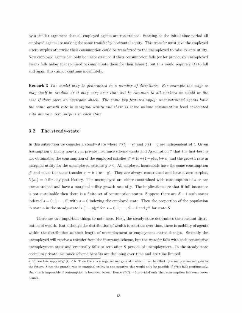
Example 1 The solution when u(c) = v(c) = loge(c), b = 1, w = 3, p = 12 , δ = 1

2 , is c0 = 3.11796,

g = 0.34132 and S = 4. The steady-state distribution is drawn in Figure 1 with c1 = c0g , c2 = c1

g = c0g2

etc. With S = 4, the unemployed are excluded from benefits after four periods of unemployment

and the probability of an unemployed agent receiving no benefits is 2−4 = 116 .

In Section 5 where we consider the interaction between public and private insurance we will present

calculations based on the steady-state distributions just described. It is therefore important to know if

15

Figure 1: The Steady-State Solution

the optimum contract converges to a non-trivial steady-state. Although we have not been able to obtain a

general result we have been able to construct examples where the optimum private insurance scheme does

indeed converge to the non-trivial steady-state. To show that it can converge to the non-trivial steady-

state, consider a simple example where S ≤ 2. At date t = 1 the initial distribution has a proportion p

with unemployed and receiving cu(1) and a proportion (1− p) who are employed and receiving ce(1). In

the example it is shown that for all subsequent periods S = 2, (1 − p) are employed with consumption

ce(t), p(1−p) are in their first period of disability receiving cu(t) and the remaining proportion p2 have a

longer term unemployment and have a consumption of b. The employed are constrained in each period.

The aggregate constraint at date t = 1 is

(1− p)ce(1) + pcu(1) = b+ (1− p)w

and the aggregate constraint for t > 1 is

(1− p)ce(t) + p(1− p)cu(t) + p2b = b+ (1− p)w.

Given these aggregate constraints, we have a dynamic equation for cu(t) given by

u(w +b− pcu(1)(1− p)

)− u(b+ w) + δp(v(cu(2))− v(b)) = 0

and for t > 1

u(w + (1 + p)b− pcu(t))− u(b+ w) + δp(v(cu(t+ 1))− v(b)) = 0.

16

The dynamic equation is

cu(t+ 1) = v−1(

v(b) +u(b+ w)− u(w + (1 + p)b− pcu(t))

δp

)

.

Differentiation shows that dcu(t+1)dcu(t) > 0 and d2cu(t+1)

d(cu(t))2 > 0. There is a unique (non-zero) stationary point

which by the convexity is unstable. Clearly any unstable path is inefficient or violates a self-enforcing

constraint, therefore consumption will be chosen at the stable point from t > 1. The next example shows

that it is possible to construct the exact solution for the optimum private insurance scheme in a simple

case.

Example 2 b = 1,w = 3,p = 12 , δ =

25 , u(c) = v(c) = loge(c). Then

cu(t+ 1) = e5(loge(4)−loge(92−

12 cu(t))).

ce(t) = 3.45 for all t ≥ 1, cu(1) = 1.55 and cu(t) = 2.1 for all t > 1.

4 Public Unemployment Insurance

In this section we use the model of Section 2 to outline the analysis of public unemployment insurance

given by Diamond and Mirrlees (1978). This is then used in the next section where the interaction

between the public and private insurance schemes is studied. Unlike the private insurance scheme of

Section 3, shirking is important because it is assumed that the government is unable to tell whether

an agent can work or not but only if they do work or not. Hence the public insurance scheme must

respect a moral hazard constraint that agents who can work do work. Also unlike private insurance

arrangements, taxes, i.e., payments into the scheme, can be enforced by the government.

The public insurance scheme is assumed to be history independent and revenue neutral. The gov-

ernment chooses the tax θ for the employed and level of subsidy σ for the unemployed that determine

the consumption levels ce = b + w − θ and cu = b + σ for the employed and unemployed respectively.

As there is a continuum of agents and the probability of that an agent can work is independent, revenue

neutrality implies that the following aggregate resource constraint is met:

(1− p)θ = pσ. (7)

It is assumed that σ ≥ 0 as consumption cannot fall below the subsistence level of b. Since the government

is unable to determine why an agent does not work—are they shirking or are they unable to work—its

policy must also respect the moral hazard constraint that an agent who can work has no incentive to

shirk rather than working,

u(b+ w − θ) ≥ v(b+ σ). (8)

17

Thus we have:

Definition 3 A public insurance scheme is a subsidy σ ≥ 0 paid to the employed from a tax θ ≥ 0

paid by the employed where σ and θ satisfy equations (7) and (8).

The additional aggregate social welfare created by the scheme over autarky is

(1− p)(u(b+ w − θ)− u(b+ w)) + p(v(b+ σ)− v(b)). (9)

We assume that the government wants to choose σ ≥ 0 and θ ≥ 0 to maximize this aggregate social

welfare.

Definition 4 The optimum public insurance scheme is the public insurance scheme that max-

imises social welfare (9).

The main result on public insurance is given by Diamond and Mirrlees (Diamond and Mirrlees 1978).

Theorem 2 (Diamond-Mirrlees) If u(ce) = v(cu) implies u′(ce) ≤ v′(cu) for all ce and cu, then

the optimum is determined by the solution to u(b + w − θ) = v(b + σ) and the budget balance

condition (1− p)θ = pσ.

Henceforth we will maintain the assumption that the moral hazard constraint of equation (8) binds.

Assumption 9 The gorvernment’s moral hazard constraint binds: u(ce) = v(cu) implies u′(ce) ≤

v′(cu) for all ce and cu.

The Diamond-Mirrlees solution is easy to envisage in (cu, ce)-space. The autarkic allocation is at

the point (b, b + w). To transfer one unit to each of the unemployed (of which there is a proportion p)

requires each of the employed (of which there is a proportion (1−p)) to give up p/(1−p) units. Thus the

slope of the aggregate budget constraint is p/(1− p). The social welfare function is (1− p)(u(ce)− u(b+

w)) + p(v(cu) − v(b)) and the slope of the social indifference curve is pv′(cu)/(1 − p)u′(ce), so tangency

occurs at a point where v′(cu) = u′(ce). By Assumption 8 at the first-best optimum the employed get no

less than the unemployed, so that the v′(cu) = u′(ce) locus lies above the 450 line. The Diamond-Mirrlees

solution is at the intersection of the budget constraint and the u(ce) = v(cu) locus which lies above the

v′(cu) = u′(ce) locus by Assumption 9 that the moral hazard constraint binds.

18

5 Crowding Out

In this section we examine both the public and private insurance schemes together. The questions we

address are: How do the public and private insurance schemes interact? Does public insurance crowd out

private insurance? And can it be optimal to have a mix of public and private insurance?

To do this we bring together the analysis of Section 3 and Section 4. We consider the effect on

the steady-state of the private insurance scheme from a government insurance scheme of the Diamond-

Mirrlees type. The public insurance scheme will affect the private insurance provision by changing the

fall-back utility of both the employed and unemployed. The public insurance will provide some risk-

sharing gains by reducing the variability of marginal utility for the employed and unemployed. However,

in achieving these risk-sharing gains, the public insurance will make the punishment of removal of future

private insurance from anyone who reneges on their private insurance payments less severe, and therefore

may reduce the risk-sharing achieved by the private insurance arrangement itself. Thus it is unclear a

priori which effect may dominate or whether a combination of public and private insurance may be

optimal.

In addition to the assumption that the government cannot observe whether an agent can work, it is

assumed that the government cannot observe the workings of the private insurance arrangement (i.e. it

cannot observe the consumption of agents), but can only observe an agent’s employment status. Thus

the tax or subsidy can only be based on employment status and not consumption. Further we analyse

a static public insurance where tax or subsidy depends only on current employment status. Thus the

public insurance scheme we consider here is of the same form as that examined in Section 4. It is simply

a tax on the employed of θ ∈ [0, w] and a subsidy to the unemployed of σ. It is assumed that the public

insurance is revenue neutral. Given that the moral hazard problem is solved, so that the fraction of the

population unemployed is indeed p, the condition for revenue neutral insurance is as before (1−p)θ = pσ.

For given (σ, θ), the private insurance scheme will solve exactly the same problem as given in Section

3, except that autarky consumption in the employment state is now ce = b + w − θ, and in the unem-

ployment state it is cu = b + σ. The relevant moral hazard constraint of the government is that of a

worker in the private insurance scheme but contemplating shirking and collecting government unemploy-

ment insurance even though able to work. Such an agent will be observed as shirking by his fellows and

therefore will receive no future benefits from the private insurance arrangement.19 We now show that

the moral hazard constraint for the government is indeed equation (8) of Section 4 even in presence of a

private insurance scheme. This is a non-trivial result which follows from Theorem 1 that U(ht) = 0 so

19We are ruling out the possibility that agents in the private scheme collude so that some of them shirk. Note that

Assumption 5 has already ruled out random schemes from consideration.

19

that every employed worker has a zero surplus. This result greatly simplifies the subsequent analysis.

Theorem 3 The moral hazard constraint in the model with both public and private insurance is

given by (8), i.e., it is the same as in the model with only public insurance:

u(b+ w − θ) ≥ v(b+ σ).

Proof: Consider an employed agent in the private insurance arrangement who is contemplating shirking

to take advantage of the government subsidy to the unemployed. As demonstrated in Theorem 1 an

employed worker at t receives a surplus of U(ht−1) = 0, where the surplus is now measured relative

to what they would have outside the private insurance scheme, i.e. b + w − θ for the employed and

b+ σ for the unemployed. If an agent shirks, the fellow members of the private insurance scheme would

recognize this and pay no subsidy. Thus the current utility gain over autarky to the agent would be

v(b+ σ)− u(b+w− θ). By assumption, the agent would be barred from the private insurance scheme in

the future and therefore would be reliant solely on government insurance. If the constraint were satisfied,

then as we have already shown, an agent solely in the public insurance scheme will have no incentive to

shirk and thus the net gain relative to autarky will be zero. Thus if v(b+σ)−u(b+w− θ) ≤ 0 the agent

will have no incentive to shirk. If however, v(b+σ)−u(b+w− θ) > 0 the agent would have an incentive

to shirk both inside and outside the private insurance scheme as U(ht−1) = 0. Thus equation (8) is a

necessary and sufficient condition for no agent to have an incentive to shirk at any date. ‖

Remark 4 Since the moral hazard constraint is the same whether an agent is receiving private

insurance or not our analysis also applies to the situation where there is some fraction of agents

outside the private insurance scheme. Thus it is possible to undertake a welfare analysis of the

effect of public insurance even when only a fraction of the agents participate in private insurance.

Clearly the smaller the fraction of the population that are members of a private insurance scheme,

the greater the weight that will be given to public insurance.

Remark 5 In line with Section 4, we do not consider negative taxes, i.e. taxation of the unem-

ployed. Although there is a lower bound on consumption of b, negative taxes may be feasible if it

could be guaranteed that the private insurance arrangements stepped in to offset any tax on the

unemployed. This would be impossible if there were some fraction of agents outside the private

insurance scheme. Since the government cannot by assumption observe whether an agent receives

private insurance, we rule out negative taxes as infeasible.

We now consider the optimality of public insurance when private insurance is possible. It is easy to

construct examples such that for certain parameter values, public insurance alone will be optimal and

20

for other parameter values private insurance will be optimal. From Assumption 6 it is known that there

will be no private insurance if the risk-sharing gains are sufficiently small, i.e. if the discount factor, δ is

sufficiently small or if the probability, p is sufficiently high. Thus if the parameter values are such that

no private insurance is feasible, and the government’s moral hazard constraint does not bind when there

is no private insurance, then it is possible to raise welfare through public insurance alone. If the moral

hazard constraint binds before any private insurance becomes feasible, then public insurance alone will

be optimal. Equally if the discount factor is high enough that the first-best can be sustained by private

insurance, then private insurance alone will achieve the optimum as by Assumption 9 the government is

constrained from achieving the first-best by the moral hazard constraint.

Since it is difficult to obtain analytical results and since we know that either public or private

insurance alone can be optimal, we simply construct numerical examples to show two further possibilities.

To do this we examine how steady-state welfare changes as the government changes the public insurance

tax. First we construct an example to show that the government can inadvertently lower welfare by

increasing public insurance, so that there is more than one-for-one crowding out of private insurance.

Secondly, an example is constructed where a combination of public insurance and private insurance can

actually raise welfare.

For simplicity we will consider the case where u(c) = v(c)− x = loge(c)− x where x is the disutility

of labour. The aggregate welfare generated by the public insurance relative to autarky is:

(1− p)(loge(b+ w − θ)− loge(b+ w)) + p(loge(b+ σ)− loge(b))

where σ = (1−p)p θ. This aggregate welfare is increasing in θ given Assumptions 4 and 9. The moral

hazard constraint in this case is

loge(w + b− θ)− loge(b+ σ) ≥ x

and this will limit the tax θ that can be imposed on the employed. The aggregate social welfare in the

steady-state generated by private insurance relative to the fall back of only public insurance is

(1− p)(loge(c0)− loge(b+ w − θ))+S−1∑

s=1

(1− p)ps(loge(c0)− loge(b+ σ)− s loge(1 + g)).

The steady-state for the private insurance can be computed as described in Subsection 3.2 and the net

welfare from public insurance and private insurance calculated for different values of public taxation θ.

The total welfare can then be computed20 and for the purposes of comparison these welfare computations

20It is assumed that only a fraction of agents of measure zero are outside the private insurance scheme in the calculations

below.

21

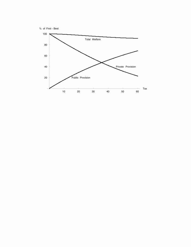
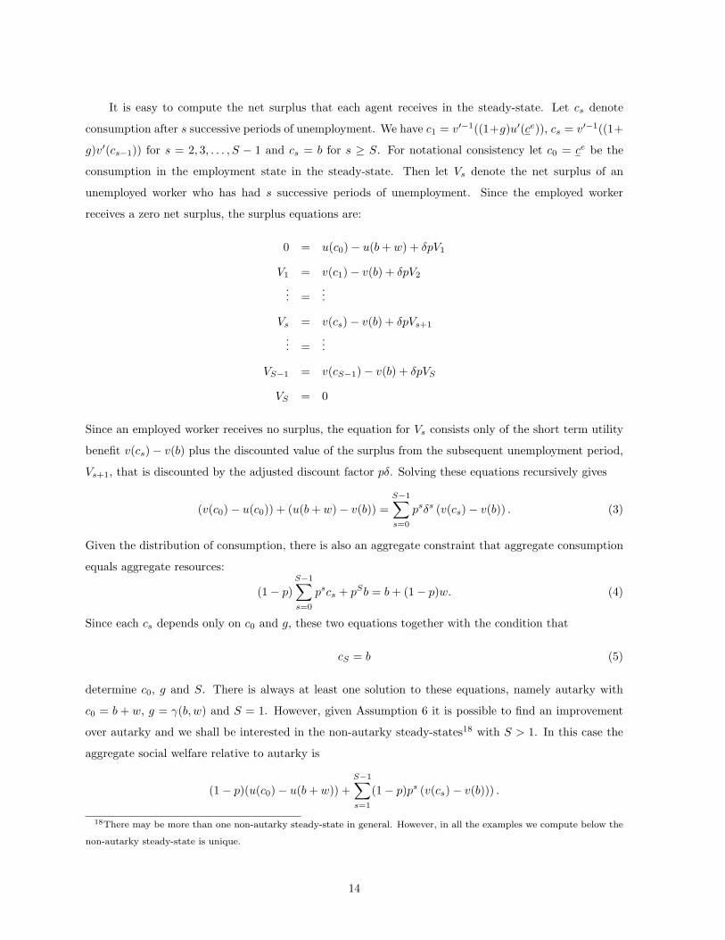
10 20 30 40 50 60Tax

20

40

60

80

100

% of First - Best

Total Welfare

Private Provision

Public Provision

Figure 2: The Crowding-Out Effect

are expressed as a percentage of the first-best welfare relative to autarky. The next two examples, together

with the associated Figures 2 and 3 show that there can be more than one-for-one crowding out and that

a mixture of private and public insurance may dominate either public or private insurance alone.

Example 3 Suppose u(c) = v(c) − x = loge(c), b = 100, w = 300, p = 12 , δ = 2

3 , x = loge(178 ). The

welfare from public and private insurance and total welfare for different values of tax (consistent

with the moral hazard constraint) is plotted in Figure 2. The maximum tax is θ = 60. At

θ = 60, the public insurance scheme generates 68.90% of the first-best surplus. At this tax rate,

the private insurance generates an additional 22.63% of the first-best surplus. Thus the public and

private insurance schemes together generate 91.53% of the first-best surplus. At θ = 0 the private

insurance scheme alone generates 99.88% of the first-best surplus. So the optimum is to have no

public insurance and have only private arrangements provide unemployment insurance.

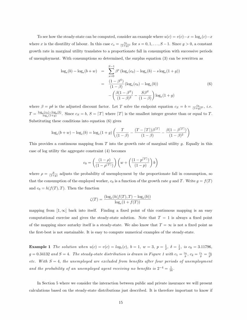
Example 4 Suppose u(c) = v(c) − x = loge(c), b = 515, w = 125, p = 45 , δ = 19

20 , x = loge(58/53).

The aggregate welfare for different values of tax is plotted in Figure 3. With x = loge(5853 ) the

maximum tax is θ = 60. At θ = 60, the public insurance scheme generates 83.21% of the first-best

surplus. At this tax rate, the private insurance generates an additional 9.66% of the first-best

surplus. Thus the public and private insurance schemes together generate 92.87% of the first-best

surplus. At θ = 0 the private insurance scheme alone generates 89.70% of the first-best surplus

but still less than that achieved with the maximum tax rate of θ = 60.

22

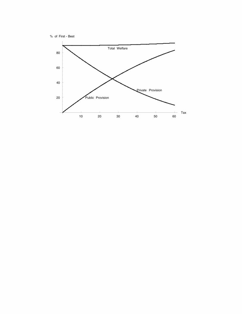
10 20 30 40 50 60Tax

20

40

60

80

% of First - Best

Total Welfare

Private Provision

Public Provision

Figure 3: An Optimal Mix of Public and Private Insurance

6 Conclusion

We have considered a model of the interaction between private and public insurance schemes. The

advantage of the private insurance scheme is that it does not have the moral hazard constraint faced

by government. However, the disadvantage of the private insurance scheme is that it cannot enforce

payments into the scheme in the way the government scheme can.

We have developed a model of private insurance in a continuum economy using straightforward

arbitrage arguments. The optimum private insurance scheme has a number of interesting properties.

First, at any date t it is described by only two numbers, the tax paid by the employed and the growth

rate in marginal utility for those unemployed workers receiving a benefit from the scheme. Thus the

optimal scheme is history dependent for the unemployed but history independent for the employed. In

a steady-state the amount received by the employed falls with the length of unemployment and is time

limited. After a certain length of unemployment no insurance benefits are received.

We have shown that there can be more than one-for-one crowding out of private insurance by public

insurance. That is a government that introduced additional public insurance may end up lowering welfare

because it crowds out even more private insurance. We have also demonstrated by way of example that

a mixture of public and private insurance may maximise steady-state welfare.

There remains work for further research. We have considered only the impact of the public insurance

on the steady-state. It would be interesting to understand how welfare changes along any dynamic path

23

toward a steady-state (though since the steady-state is feasible our calculations place a lower bound on

the welfare gain due to private insurance). Further, the government in contrast to the private sector

is assumed to adopt a static taxation system that depends only on the current employment status and

not the employment history. Many government insurance schemes are responsive to employment history

and exhibit some features such as declining and time limited benefits that we have found to optimal in

the private insurance scheme. Again future research could address how a dynamic model of government

insurance interacts with private insurance. Further in our model unemployment is exogenous and not

affected by agents’ decisions. Examining the welfare consequences in a model where the extent of insurance

had an impact on the level of unemployment could provide an interesting extension of the model.

24

Appendix

The appendix proves Theorem 1. To do so we first prove Lemma 4.

Lemma 4 For a given employment status at date t ≥ 1, there is a unique consumption level which

delivers zero surplus at that date.

Proof: We first show that U(ht−1) > U(h′t−1) if and only if ce(ht−1) > ce(h′t−1) and V (ht−1) > V (h′t−1)

if and only if cu(ht−1) > cu(h′t−1). From the recursive equations

U(ht−1) = u(ce(ht−1))− u(b+ w) + δ(

(1− p)U(ht−1, et) + pV (ht−1, e

t))

U(h′t−1) = u(ce(h′t−1))− u(b+ w) + δ(

(1− p)U(h′t−1, et) + pV (h′t−1, e

t))

First we prove sufficiency. Suppose by contradiction we have U(ht−1) > U(h′t−1) but ce(ht−1) ≤ ce(h′t−1).

Then

(1− p)U(ht−1, et) + pV (ht−1, e

t) > (1− p)U(h′t−1, et) + pV (h′t−1, e

t)

Thus either U(h′t−1, et) < U(ht−1, e

t) or V (h′t−1, et) < V (ht−1, e

t) or both. It is only possible to have

higher surplus if at some future point consumption is higher, so w.l.o.g. take this to be period t + 1.

Suppose by way of example that we have V (ht−1, et) > V (h′t−1, e

t) ≥ 0 and cu(h′t−1, et) < cu(ht−1, e

t).

But then by risk aversionv′(cu(h′t−1, e

t))

u′(ce(h′t−1))>v′(cu(ht−1, e

t))

u′(ce(ht−1)).

This implies that (ht−1, et) has a smaller marginal utility growth rate and thus that V (ht−1, e

t) = 0 by

Lemma 3 which contradicts V (ht−1, et) > 0. A similar argument applies if U(ht−1, e

t) > U(h′t−1, et) ≥ 0.

To prove necessity again suppose by contradiction that ce(ht−1) > ce(h′t−1) but U(ht−1) ≤ U(h′t−1). By

the first part of the proof if U(ht−1) < U(h′t−1) then we have ce(h′t−1) > ce(ht−1); a contradiction. Thus

suppose that U(ht−1) = U(h′t−1). Now choose a convex combination of the contracts so that both types

get the same consumption at all dates from t onwards. By concavity this leads to a Pareto-improvement,

with all the self-enforcing constraints satisfied. Equally all self-enforcing constraints at past periods are

met or relaxed. Thus the original contract could not have been efficient. Given the strict monotonicity

it follows that there is a unique consumption level that delivers zero surplus in each employment state at

any date. ‖

Theorem 1 Given Assumptions 1-7, at any time t ≥ 1 the transition rule from time t to t + 1

is determined by two numbers b + (1 − p)w ≤ ce(t) ≤ b + w and g(t) ≥ 0 such that the transition

between states satisfies

25

1. A transition to an employment state

ce(ht−1, ut) = ce(ht−1, e

t) = ce(t+ 1).

2. A transition to an unemployment state

(a) From an unemployment state

cu(ht−1, ut) =

{

v′−1((1 + g(t+ 1))v′(cu(ht−1))), if cu(ht−1, ut) ≥ b

b, otherwise.

(b) From an employment state

cu(ht−1, et) =

{

v′−1((1 + g(t+ 1))u′(ce(t))), if cu(ht−1, et) ≥ b

b, otherwise.

Proof: First we show that the growth rate in marginal utility is non-negative. Suppose to the contrary

that g(t) < 0. This implies that for every agent marginal utility at time t is greater than the marginal

utility at time t + 1 no matter what the states at each date or whether the worker is constrained or

not. Consider a worker with history ht−1. If the history is ht+1 = (ht−1, et, et+1) then ce(ht−1, e

t) >

ce(ht−1). Likewise for the history ht+1 = (ht−1, ut, ut+1), cu(ht−1, u

t) > cu(ht−1). For the history

ht+1 = (ht−1, ut, et+1), it follows from Assumption 8 that ce(ht−1, u

t) > cu(ht−1) + k and similarly that

for the history ht+1 = (ht−1, et, ut+1), cu(ht−1, e

t) > ce(ht−1) − k. Since the probability of illness is

independent, the histories ht+1 = (ht−1, et, ut+1), and ht+1 = (ht−1, u

t, et+1), are equally likely. Thus

summing over all possible histories ht−1, it follows that aggregate consumption rises from time t to t+1,

but this is impossible as aggregate resources are unchanged. Thus we conclude that g(t) ≥ 0. Next it has

been demonstrated in the text that at any time t, b < ce(t) ≤ b + w and cu(t) = b so that constrained

agents who employed consume ce(t) and that constrained unemployed agents consume b. It has also

been shown in Lemmas 2 and 3 that unconstrained agents have higher consumption and a growth rate

in marginal utility of g(t). It only remains to show that all employed agents are constrained and hence

consume ce(t). To see this suppose that the employed at t − 1 are all constrained: U(ht−2) = 0 for all

ht−2. To show that the employed at t are constrained, first assume that some who are employed both at

t − 1 and t have marginal utility growth equal to g(t) that is u′(ce(ht−2, et−1))/u′(ce(ht−2)) = 1 + g(t)

for some ht−2. We show this is impossible, and hence all such agents must be constrained at t. First, the

growth rate must be the same in the unemployment state at t: v′(cu(ht−2, et−1))/u′(ce(ht−2)) = 1+ g(t)

since otherwise cu(ht−2, et−1) = b, by the above argument and hence u′(ce(ht−2, e

t−1)) > v′(b), which is

impossible. Suppose without loss of generality that thereafter, as soon as the employed state occurs, say

at any time t′ ≥ t+1, total surplus discounted to t′ will be zero, i.e., U(ht−2, et−1, st, ut+1, . . . ut

′−1) = 0

26

(where st ∈ {ut, et}). This is w.l.o.g. as we can consider the path where u is repeated from date t, until

the last time that

v′(ce(ht′−2, et−1, st, ut+1, . . . , ut

′′−1))/u′(cu(ht′−2, et−1, st, ut+1, . . . , ut

′′−2)) = 1 + g(t′′).

Thereafter, by definition, as soon as the employed state occurs, total surplus will be zero. We can

use t′′ to replace t. To simplify notation, define per-period surpluses Set−1 = u(ce(ht−2)) − u(w + b),

Set = u(ce(ht−2, et−1)) − u(w + b) and likewise Sut′ = v(cu(ht−2, e

t−1, ut, . . . , ut′−1)) − v(b) for all t′ ≥ t

(t′ − t − 1 periods of unemployment after t − 1). Note that the surplus from t + 1 on is the same after

both histories (ht−1, et) and (ht−1, u

t), since marginal utilities are the same at t by assumption, and the

transition from t to t + 1 depends only on marginal utility at t. Define Z to be the total surplus from

t+ 1 onwards:

Z = pSut+1 + δp2Sut+2 + δ2p3Sut+3 . . . (10)

(using the fact that after date t an employment state implies total surplus from that point is zero). We

have by virtue of U(ht−2) = 0,

−Set−1 = (1− p)δU(ht−2, et−1) + p

(

δSut + δ2Z)

≥ p(

δSut + δ2Z)

(11)

where the inequality follows from U(ht−2, et−1) ≥ 0. By U(ht−2, e

t−1) ≥ 0,

−Set ≤ δZ. (12)

In view of Sut′+1 ≤ Sut′ for all t′ ≥ t due to g(t′ + 1) > 0 (no first-best), we have Sut ≥ Sut′ for all t′ > t.

From (10), this implies pSut /(1− δp) > Z. Hence

p(

δSut + δ2Z)

> δZ (13)

We also have Set−1 > Set due to g(t′ + 1) > 0. Using this and combining the inequalities of (11), (12)

and (13), we have −Set−1 ≥ p(

δSut + δ2Z)

> δZ ≥ −Set > −Set−1, a contradiction. Since the initial time

period has all employed agents making the same transfer, this transfer must be such that the employed

initially have a zero net surplus and this completes the proof. ‖

27

References

Arnott, R., and J. E. Stiglitz (1991): “Moral hazard and nonmarket institutions: Dysfunctional

crowding out or peer monitoring?,” American Economic Review, 81, 179–190.

Atkeson, A., and R. E. Lucas (1992): “On efficient distribution with private information,” Review

of Economic Studies, 59, 427–453.

Attanasio, O., and J.-V. Rios-Rull (2000): “Consumption smoothing in island economies: Can

public insurance reduce welfare?,” European Economic Review, 44, 1225–1258.

Coate, S., and M. Ravallion (1993): “Reciprocity without Commitment: Characterisation an Per-

formance of Informal Insurance Arrangements,” Journal of Development Economics, 40, 957–976.

Di-Tella, R., and R. MacCulloch (2002): “Informal Family Insurance and the Design of the Welfare

State,” Economic Journal, 112, 481–503.

Diamond, P. A., and J. A. Mirrlees (1978): “A model of social insurance with variable retirement,”

Journal of Public Economics, 10, 295–336.

Kreuger, D., and F. Perri (1999): “Risk sharing: Private insurance markets or redistributive taxes?,”

Mimeo.

Ligon, E., J. P. Thomas, and T. Worrall (2000): “Mutual insurance, individual savings and limited

commitment,” Review of Economic Dynamics, 3(2), 216–246.

(2002): “Informal insurance arrangements with limited commitment: Theory and evidence from

village economies,” Review of Economic Studies, 69(1), 209–244.

Thomas, J. P., and T. Worrall (1988): “Self-enforcing wage contracts,” Review of Economic

Studies, 55(4), 541–554.

28