UNIVERSITY OF NOTTINGHAM Discussion Papers in Economics ___________________________________________________ Discussion Paper No. 09/02 Unemployment Duration in the United Kingdom: An Incomplete Data Approach By Ralf A. Wilke February 2009 __________________________________________________________________ 2009 DP 09/02

Welcome message from author
This document is posted to help you gain knowledge. Please leave a comment to let me know what you think about it! Share it to your friends and learn new things together.
Transcript
UNIVERSITY OF NOTTINGHAM
Discussion Papers in Economics
___________________________________________________ Discussion Paper No. 09/02
Unemployment Duration in the United Kingdom: An Incomplete Data Approach
By Ralf A. Wilke
February 2009 __________________________________________________________________ 2009 DP 09/02
Unemployment Duration in the United Kingdom:
An Incomplete Data Approach ∗
Ralf A. Wilke†
February 2009
Abstract
For the evaluation of policy reforms numerous governments use, among other sources,
administrative social security data. Although this data is large and contains detailed in-
formation about policy measures, it inherits several limitations due to the administrative
process of generating data. This paper explores the implications of missing interval infor-
mation in data from the UK (JUVOS) for the analysis of unemployment duration. Variants
of the JUVOS are used by the labour administration and the research community as an
important source for the analysis of unemployment. While previous work has mentioned the
relevant data limitations, they were not taken into account in the empirical approaches. The
econometric analysis in this paper shows that competing implementations of unemployment
duration in the data yield partly unstable empirical result pattern even in presence of a huge
number of observations.
Keywords: Administrative Data, Missing Information, Competing Risks
JEL: C41, J64
1 Introduction
Since the late 1990s, several European governments, lead by the Nordic states, have been making
efforts to make administrative individual spell data accessible. This data can contain information
∗I thank Nirmalathevy Vijayakumar (Office for National Statistics) and Will Driskell (Department for Work
and Pensions) for their help with the data and I am grateful for the comments of the participants at numerous
seminar talks. This work is supported by the Economic and Social Research Council through the grant Bounds for
Competing Risks Duration Models using Administrative Unemployment Duration Data (RES-061-25-0059).†University of Nottingham, School of Economics, University Park, Nottingham NG7 2RD, UK, E-mail:

from several administrative registers which are merged with the help of an individual’s national
insurance number. Recently, it has been extensively used to evaluate reforms of the social security
system on behalf of national governments. For this purpose the UK Department for Work and
Pension (DWP) has access to several administrative registers (e.g. benefit claimants, tax records).
There are several variants of merged administrative data in the UK. The most comprehensive is the
Work and Pensions Longitudinal Study (WPLS) which was released in 20041. This data base plays
an important role for the internal processes in the UK public labour administration. Moreover,
the DWP carries out internal and contracted research to evaluate a variety of policy measures.
This currently includes research on many aspects such as disability benefits or child benefits (see
DWP, 2008 and Kossigh, Walker and Zhu, 2008). In some cases, the benefit data is also merged
with household interview data, see for example Green at al. (2003) or Bryson and Kasparova
(2003). Interview data can add valuable information which is not available from administrative
sources. Access to administrative individual data is restricted due to data protection clauses and
access to WPLS cannot be granted for independent researchers. Academic research is therefore
restricted to scientific use files but they are available in few cases only. Since the early 1990s
various household surveys have been used to explore the determinants of unemployment duration.
Among others, the Family Expenditure Survey, the British Labour Force Survey and the British
Household Panel Survey are the most prominent survey data sets. In the second half of the 1990s,
British administrative data on individual level emerged in academic research as an alternative
to survey data (e.g. van den Berg and van Ours, 1994, Dolton and O’Neill, 2002). This data
was made available more broadly in 1995, when the British government released the JUVOS
(Joint Unemployment and Vacancies On-Line System) cohort. The JUVOS is a scientific use
file which contains a 5% sample of unemployment related benefits claimants (Ward and Bird,
1995). Various versions have been used in studies to analyse the duration of unemployment in
the UK (e.g. Kalwij, 2004, McVicar and Podivinsky, 2002 and 2003). As it also contains some
information about the assignment into training and active labour market programmes (ALMP),
the data has also been used to evaluate the effect the New Deal programme for young people
has on unemployment duration. See again McVicar and Podivinsky for more details. Blundell,
Costa Dias, Meghir and Van Reenen (2004) mainly base their empirical analysis of the evaluation
of the New Deal programme on the JUVOS, while their work does not contain an analysis of
unemployment duration. These references indicate the importance of the JUVOS as a tool to
investigate the effects of policy reforms on UK unemployment.
Administrative individual spell data has the advantage that it usually contains a huge number
of observations and important variables, such as benefit claim periods, are measured without recall
1For more information see http : //www.dwp.gov.uk/asd/longitudinal study/ic longitudinal study.asp.
2
errors (Machin and Manning, 1999). However, it has also several limitations. It contains only
few household background variables and there are considerable unobserved periods in individual
employment biographies. Interval information is missing if it is not covered by the administra-
tive processes and in many cases this leads to an ambiguity regarding the labour market state.
Unemployment duration is then only partly observed and different implementations of unemploy-
ment in the data yield different number and length of unemployment spells. See Kruppe, Muller,
Wichert and Wilke (2008) for the case of German merged administrative data. This can result
in instability of empirical result patterns (Fitzenberger and Wilke, 2004) and therefore in a gen-
eral difficulty for the interpretation of empirical results (Card, Chetty and Weber, 2007). More
formally, Lee and Wilke (2008) and Arntz, Lo and Wilke (2007) bound the treatment effect of
changes in unemployment benefit entitlement lengths on unemployment duration over different
implementations of unemployment duration in German administrative data. Their bounds are due
to unobserved periods in the data and do not disappear even when the sample size goes to infinity.
The resulting bounds of their analysis can be rather wide and preclude any causal inference even
in presence of a large number of observations and exact information about the policy measure.
This is the motivating starting point of this work which aims in analysing similar data problems
in UK administrative data which have not been addressed yet.
Previous work using the JUVOS has usually defined one unemployment period as one claim
period and it has not explicitly accounted for unobserved periods and ambiguity regarding the
labour market state. This work
• suggests different implementations of unemployment duration in the JUVOS,
• creates a competing risks data structure although the data contains information about one
administrative register only,
• estimates non- and semiparametric econometric duration models and explores how sensitive
the estimation results are with respect to the definition of unemployment.
The paper explores the information content of the JUVOS for unemployment duration analysis
and it illustrates the implications of limited data availability for the precision of empirical results.
The results show that several empirical result patterns are not robust while others are. It therefore
depends on the specific research question at hand whether the JUVOS can be used as a reliable data
source for applied labour market research. The paper is structured as follows: section 2 describes
the data structure. Section 3 suggests several implementations of unemployment duration. The
results of the empirical analysis are presented in section 4 and section 5 summarises and concludes.
3
2 Data
We use the August 2007 edition of the Claimant Unemployment Cohort (JUVOS Cohort). This
data is available as a Scientific Use File from the Office for National Statistics (Ward and Bird,
1995). It is a 5% random sample drawn from the population of unemployment benefit claimants in
the United Kingdom. The sampling is based on the national insurance number. The core of this
spell data are daily claim periods for unemployment compensation in the period from the early
1980s until June 2007. Beside this it contains basic individual characteristics such as sex, marital
status and age, regional information and occupational information. It therefore contains much
less interesting variables compared to survey data such as the Labour Force Survey or the British
Household Panel Survey. The strength of this data is that individual unemployment trajectories
can be tracked for many years on a daily basis. There is also a variable indicating the end reason
of a claim period. This information can be used to determine the post unemployment labour
market state or to obtain a better understanding of gaps between two claim periods.
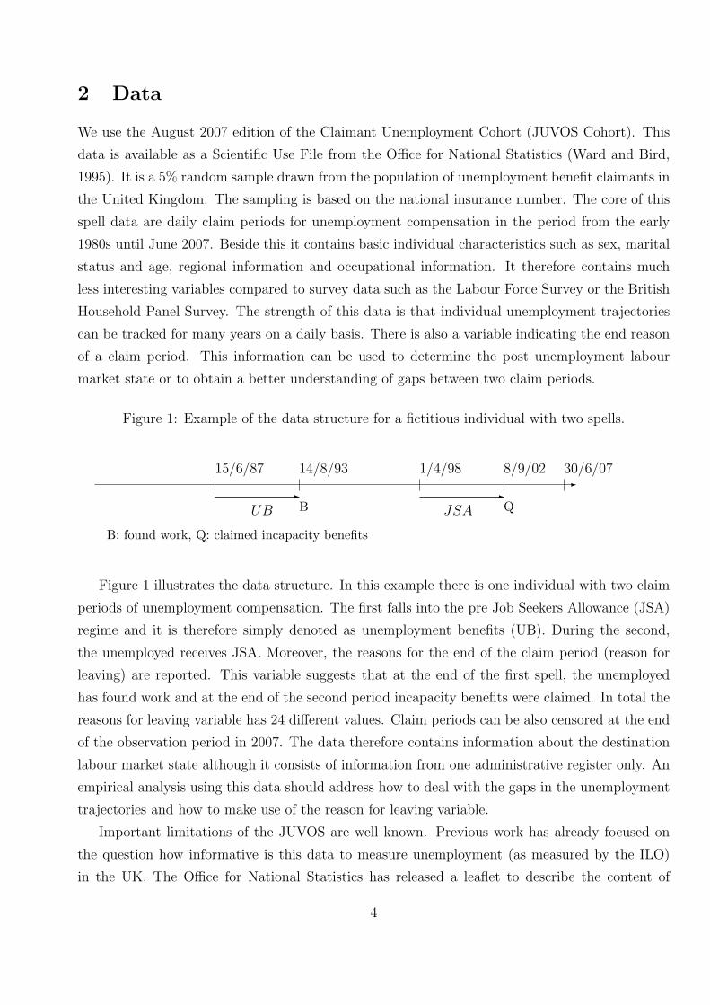
Figure 1: Example of the data structure for a fictitious individual with two spells.
-30/6/0715/6/87 14/8/93 1/4/98 8/9/02
-
UB B-
JSA Q
B: found work, Q: claimed incapacity benefits
Figure 1 illustrates the data structure. In this example there is one individual with two claim
periods of unemployment compensation. The first falls into the pre Job Seekers Allowance (JSA)
regime and it is therefore simply denoted as unemployment benefits (UB). During the second,
the unemployed receives JSA. Moreover, the reasons for the end of the claim period (reason for
leaving) are reported. This variable suggests that at the end of the first spell, the unemployed
has found work and at the end of the second period incapacity benefits were claimed. In total the
reasons for leaving variable has 24 different values. Claim periods can be also censored at the end
of the observation period in 2007. The data therefore contains information about the destination
labour market state although it consists of information from one administrative register only. An
empirical analysis using this data should address how to deal with the gaps in the unemployment
trajectories and how to make use of the reason for leaving variable.
Important limitations of the JUVOS are well known. Previous work has already focused on
the question how informative is this data to measure unemployment (as measured by the ILO)
in the UK. The Office for National Statistics has released a leaflet to describe the content of
4

the claimant counts (National Statistics, 2007). The main concern of this and related work is to
explain the divergence in the ILO unemployment rate and the unemployment rate based on claim
count data after the introduction of JSA in 1996 (see also Machin, 2004 or Manning, 2005). The
main difference is due to the fact that unemployment information in the JUVOS is only available
in case of receipt of unemployment compensation from the local jobcentre. In case an unemployed
is not eligible, she/he will not be recorded in the data. This leads to a general underreporting of
unemployment information in this data. See for example figure 1 in Machin (2004) for a time series
from 1980 until 2004. There are also cases where people can claim JSA without being unemployed
(according to the ILO definition) but it is expected that these cases are rather rare. This is the
case if their household income is low and if they work less than 16 hours per week. Eligibility
for JSA is generally based on two criteria: for the first six months, it is contribution based if the
unemployed has sufficient National Insurance contributions. In all other cases the unemployed is
eligible only after having passed a means test. After six months of unemployment, the eligibility
for JSA is income based. This implies that in particular the length of long term unemployment
periods is underreported in the JUVOS. For example long term unemployed females are probably
less likely observed in this data as they have often an employed spouse (Machin, 2004). In contrast
to many European social security systems the level of JSA is not related to the level of previous
income. Little work has been done to formally analyse the data limitations and its consequences
for duration analysis. Previous work usually assumed that one claim period is one unemployment
period and unobserved periods belong to another labour market state, mainly employment (see for
example Kalwij, 2004). In this case, information about the reason for leaving the claim period is
not used at all. Other studies make a basic distinction between employment and ALMP (McVicar
and Podivinsky, 2003). In the following we define unemployment duration in the JUVOS by taking
into account that unemployment periods are not fully observed. We make also use of the reasons
for leaving variable which contributes important information about unobserved periods in the
individual employment trajectories. This allows us to model transitions between various labour
market states such as unemployment, employment, training or out of the labour force. Moreover,
we will also address data quality issues of this variable.
A list of the reasons for leaving is given in figure 2. Due to the large number and as these
reasons do not define unique labour market states, it is difficult to use them directly for empirical
work. For this reason we make an attempt to classify five important labour market states from
the original variable coding: employment, unemployment, nonemployment, training and full-time
education. Moreover, the original coding can often not be attributed to a unique labour market
state. The colours in the table are used to distinguish between the different cases. If a reason
for leaving corresponds to a unique labour market state, it is highlighted in a specific colour to
5

Figure 2: Classification of the Reasons for Leaving Variable
6

ease the reading (see figure 2). If it is not the case, the labour market state is uncertain and
not highlighted in a colour. Note that this is a broader classification than the original coding for
”not known”. The DWP has already carried out some contract research to explore the unknown
destinations of JSA leavers (Wolstenholme, 2004). The main findings are that 50% of this group
enter employment of 16 hours or more per week. 10% are still unemployed but eligibility for JSA
has expired. 8% switch to another benefit and 6% have an interruption in their claim. Moreover,
the research shows that the probability for an unknown reason being indeed employment is lower
for unemployed which have a long period of JSA receipt. These findings show that an unknown
reason for leaving cannot be attributed to one labour market state. For this reason and to facilitate
further data preparation we group the destinations into six logical groups. These groups either
correspond to a unique labour market state or the state is unclear but it is restricted to a couple
of competing states. Note that according to DWP research, ALMP is not frequent in case of
unknown destinations. For this reason we do not allow for this state in this case. The groups of
codes are given in table 1.
Table 1: Logical groups for reason for leaving codes.
Group Original Codes Distribution
for sure unemployment L O 0.2%
for sure employment B N 49.2%
for sure training/ALMP I M 6.1%
nonemploymentaor unemployment D R 3.1%
nonemploymentaor full time education C G J Q T E 9.6%
employment/nonemploymenta/unemployment A F H S K P U V W X * 28.8%
right censored 3.0%
a out of the labour force
The percentage numbers in the third column refer to the empirical distribution for these groups
using data in the period 1997-2007. It is apparent that the codes do not uniquely identify the
destination state for about 40% of the administrative records. This number is by means not
negligible. The suggested classification forms the basis for the following implementation of unem-
ployment duration in the data and hence for the empirical analysis. Information about destination
states will be used to compute the length of unemployment periods. Moreover, it enables us to
construct a competing risks data structure. Since the reason for leaving variable is self-reported
by the unemployed, it may also be subject to measurement error. Unfortunately, the degree of
measurement error and the type are unknown. The following analysis ignores this potential issue.
7
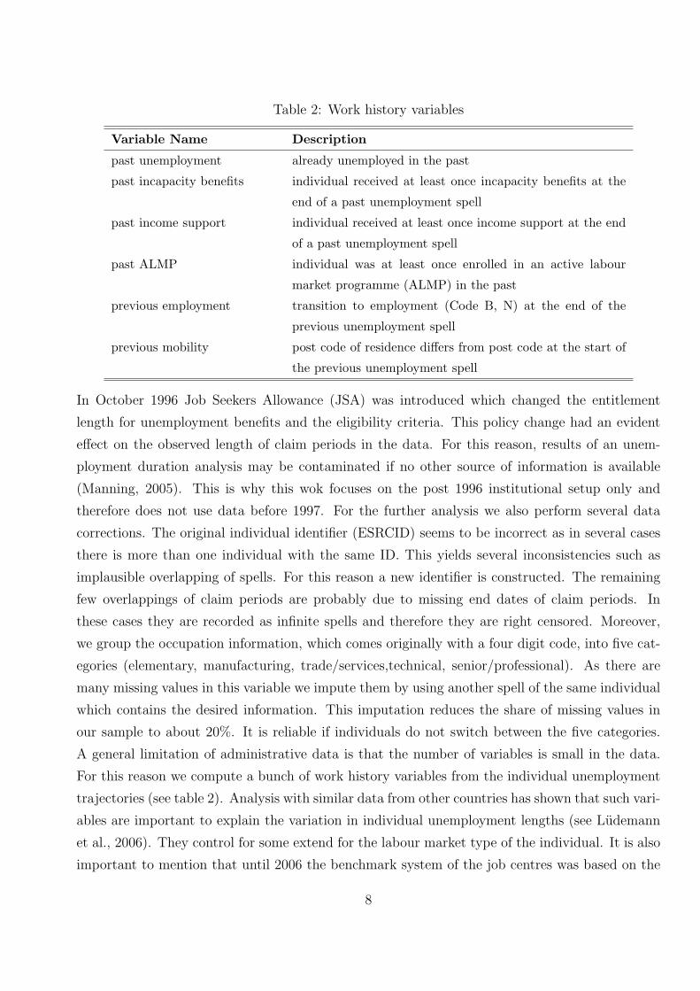
Table 2: Work history variables
Variable Name Description
past unemployment already unemployed in the past
past incapacity benefits individual received at least once incapacity benefits at the
end of a past unemployment spell
past income support individual received at least once income support at the end
of a past unemployment spell
past ALMP individual was at least once enrolled in an active labour
market programme (ALMP) in the past
previous employment transition to employment (Code B, N) at the end of the
previous unemployment spell
previous mobility post code of residence differs from post code at the start of
the previous unemployment spell
In October 1996 Job Seekers Allowance (JSA) was introduced which changed the entitlement
length for unemployment benefits and the eligibility criteria. This policy change had an evident
effect on the observed length of claim periods in the data. For this reason, results of an unem-
ployment duration analysis may be contaminated if no other source of information is available
(Manning, 2005). This is why this wok focuses on the post 1996 institutional setup only and
therefore does not use data before 1997. For the further analysis we also perform several data
corrections. The original individual identifier (ESRCID) seems to be incorrect as in several cases
there is more than one individual with the same ID. This yields several inconsistencies such as
implausible overlapping of spells. For this reason a new identifier is constructed. The remaining
few overlappings of claim periods are probably due to missing end dates of claim periods. In
these cases they are recorded as infinite spells and therefore they are right censored. Moreover,
we group the occupation information, which comes originally with a four digit code, into five cat-
egories (elementary, manufacturing, trade/services,technical, senior/professional). As there are
many missing values in this variable we impute them by using another spell of the same individual
which contains the desired information. This imputation reduces the share of missing values in
our sample to about 20%. It is reliable if individuals do not switch between the five categories.
A general limitation of administrative data is that the number of variables is small in the data.
For this reason we compute a bunch of work history variables from the individual unemployment
trajectories (see table 2). Analysis with similar data from other countries has shown that such vari-
ables are important to explain the variation in individual unemployment lengths (see Ludemann
et al., 2006). They control for some extend for the labour market type of the individual. It is also
important to mention that until 2006 the benchmark system of the job centres was based on the
8

reasons for leaving variable. Since 2006 the DWP observes an increasing number of missing values
in the reasons for leaving variable as the variable became less relevant for internal processes.
3 Definition of Unemployment
In this section we define five concepts to measure the length of an unemployment period. We
suggest lower and upper bounds of the unemployment period and several intermediate definitions.
Similar work has been done for German administrative data by Kruppe et al. (2008). The original
claim spells build the basis for this exercise. Our implementations primarily use information about
the length of interruptions between two claim periods and the destination state. If certain criteria
are satisfied, two (or more) claim spells of the same individual and the gap(s) in between form
one unemployment period. The choice of the relevant criteria determines the resulting length of
an unemployment duration:
Concept 1 Claim periods of an individual are merged if the following criteria are met. There
is a gap of less than one month in between and the reason for leaving is unemployment (codes
L, O). In case the reason for leaving cannot be uniquely classified but it is possibly related to
unemployment (codes D, R, A, F, H, S, K, P U, V, W, X, *) the gap has to be shorter than two
weeks to merge claim periods. In this concept we are conservative and only declare unobserved
periods as unemployment if they are short and if the exit reason is unemployment or related. Thus,
the computed unemployment duration should not include periods other than unemployment.
Concept 2 Based on Concept 1 we merge claim periods also in case of longer interruptions
if the exit reason is unemployment or nonemployment (codes L, O, D, R). The allowed length
of an interruption can range from one month to infinite and should be chosen according to the
preference of the researcher. This definition of unemployment also incorporates to some extent
nonemployment periods.
Concept 3 Based on Concept 2 we also merge claim periods if the exit reason is nonemployment
or full time education (codes C G J Q T E). This definition is wider as periods of full time education
(after a claim period) also contribute to the unemployment duration. This can be plausible as
not all periods of full time education are included but those which are in response to a poor
labour market outcome. For this reason these periods may be related to some form of hidden
unemployment.
9
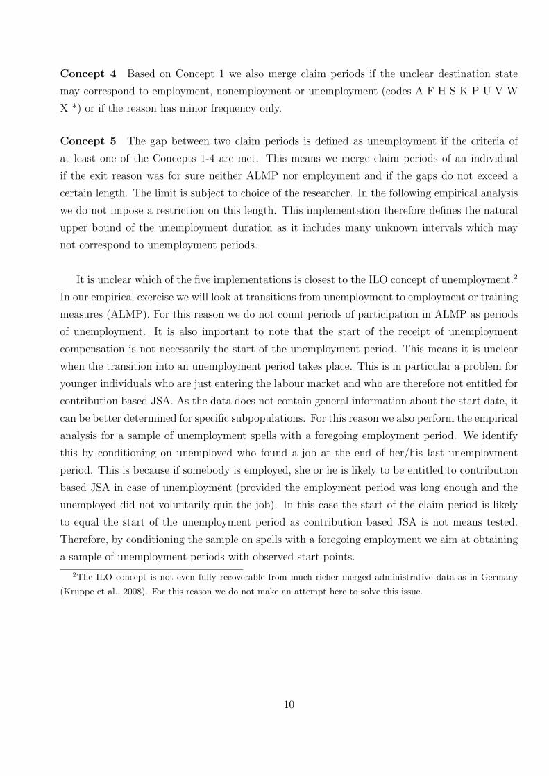
Concept 4 Based on Concept 1 we also merge claim periods if the unclear destination state
may correspond to employment, nonemployment or unemployment (codes A F H S K P U V W
X *) or if the reason has minor frequency only.
Concept 5 The gap between two claim periods is defined as unemployment if the criteria of
at least one of the Concepts 1-4 are met. This means we merge claim periods of an individual
if the exit reason was for sure neither ALMP nor employment and if the gaps do not exceed a
certain length. The limit is subject to choice of the researcher. In the following empirical analysis
we do not impose a restriction on this length. This implementation therefore defines the natural
upper bound of the unemployment duration as it includes many unknown intervals which may
not correspond to unemployment periods.
It is unclear which of the five implementations is closest to the ILO concept of unemployment.2
In our empirical exercise we will look at transitions from unemployment to employment or training
measures (ALMP). For this reason we do not count periods of participation in ALMP as periods
of unemployment. It is also important to note that the start of the receipt of unemployment
compensation is not necessarily the start of the unemployment period. This means it is unclear
when the transition into an unemployment period takes place. This is in particular a problem for
younger individuals who are just entering the labour market and who are therefore not entitled for
contribution based JSA. As the data does not contain general information about the start date, it
can be better determined for specific subpopulations. For this reason we also perform the empirical
analysis for a sample of unemployment spells with a foregoing employment period. We identify
this by conditioning on unemployed who found a job at the end of her/his last unemployment
period. This is because if somebody is employed, she or he is likely to be entitled to contribution
based JSA in case of unemployment (provided the employment period was long enough and the
unemployed did not voluntarily quit the job). In this case the start of the claim period is likely
to equal the start of the unemployment period as contribution based JSA is not means tested.
Therefore, by conditioning the sample on spells with a foregoing employment we aim at obtaining
a sample of unemployment periods with observed start points.
2The ILO concept is not even fully recoverable from much richer merged administrative data as in Germany
(Kruppe et al., 2008). For this reason we do not make an attempt here to solve this issue.
10
4 Empirical Analysis
In this section we present some exploratory evidence to which extent the different data prepa-
ration steps imply sensitivity of the empirical results. First, we will focus on the number of
unemployment spells and the distribution of destination states. Then we will analyse the dura-
tion of unemployment by means of several econometric methods. To facilitate the reading we will
present results for the lower and upper bound of the unemployment duration (Concepts 1 and 5)
only.
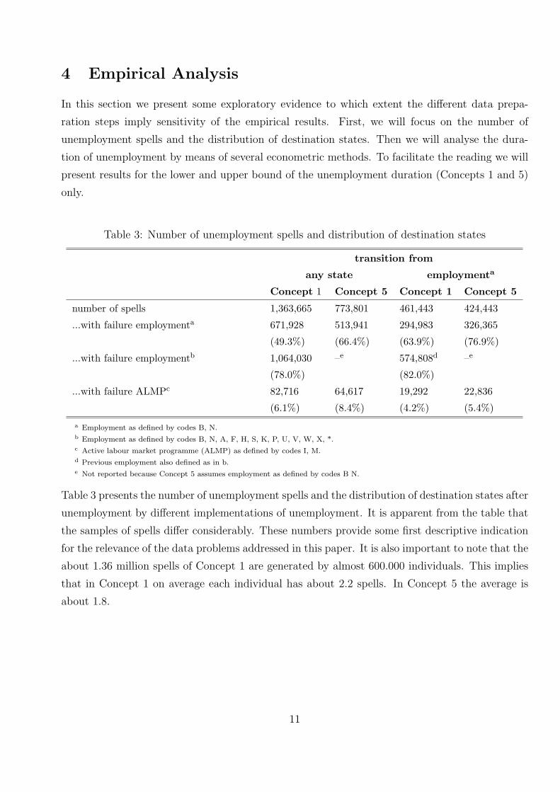
Table 3: Number of unemployment spells and distribution of destination states
transition from
any state employmenta
Concept 1 Concept 5 Concept 1 Concept 5
number of spells 1,363,665 773,801 461,443 424,443
...with failure employmenta 671,928
(49.3%)
513,941
(66.4%)
294,983
(63.9%)
326,365
(76.9%)
...with failure employmentb 1,064,030
(78.0%)
–e 574,808d
(82.0%)
–e
...with failure ALMPc 82,716
(6.1%)
64,617
(8.4%)
19,292
(4.2%)
22,836
(5.4%)
a Employment as defined by codes B, N.b Employment as defined by codes B, N, A, F, H, S, K, P, U, V, W, X, *.c Active labour market programme (ALMP) as defined by codes I, M.d Previous employment also defined as in b.e Not reported because Concept 5 assumes employment as defined by codes B N.
Table 3 presents the number of unemployment spells and the distribution of destination states after
unemployment by different implementations of unemployment. It is apparent from the table that
the samples of spells differ considerably. These numbers provide some first descriptive indication
for the relevance of the data problems addressed in this paper. It is also important to note that the
about 1.36 million spells of Concept 1 are generated by almost 600.000 individuals. This implies
that in Concept 1 on average each individual has about 2.2 spells. In Concept 5 the average is
about 1.8.
11
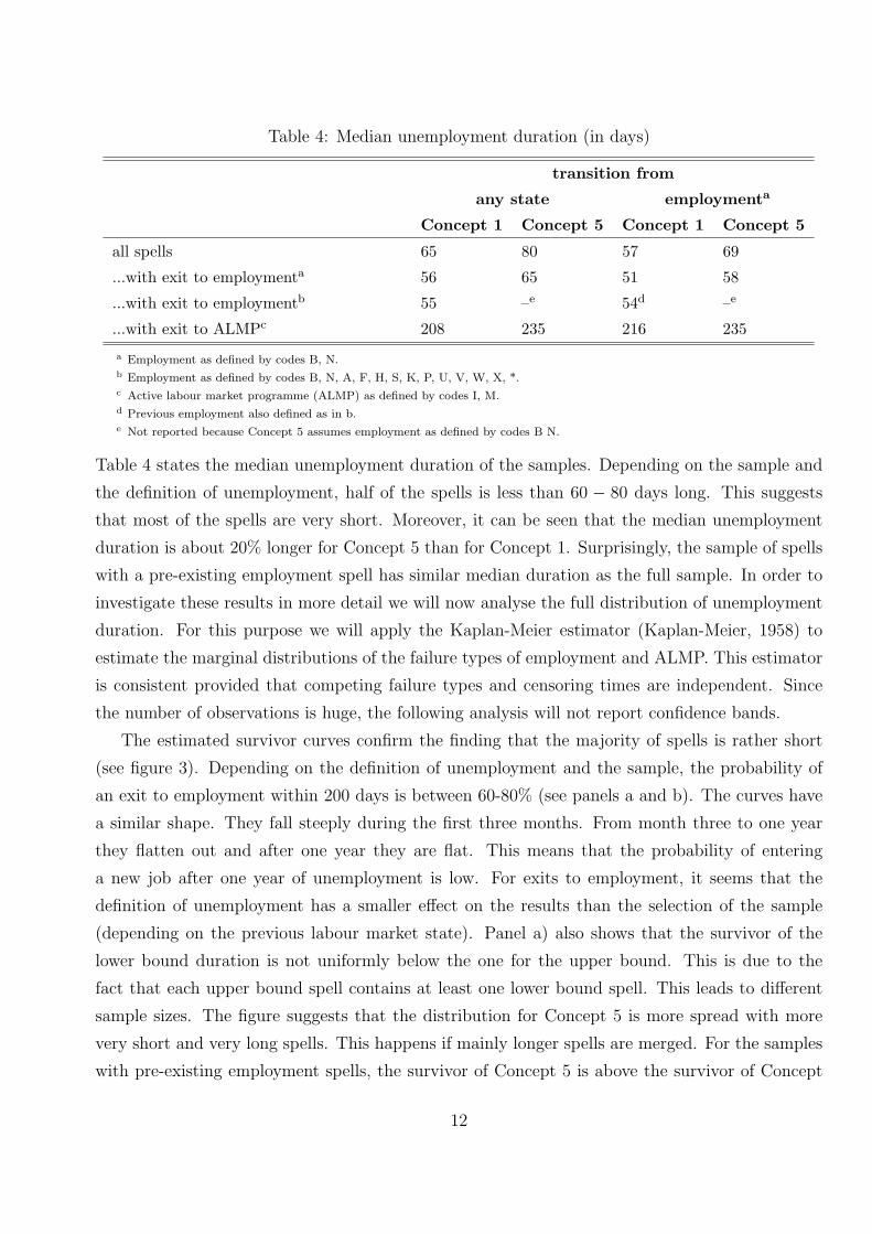
Table 4: Median unemployment duration (in days)
transition from
any state employmenta
Concept 1 Concept 5 Concept 1 Concept 5
all spells 65 80 57 69
...with exit to employmenta 56 65 51 58
...with exit to employmentb 55 –e 54d –e
...with exit to ALMPc 208 235 216 235
a Employment as defined by codes B, N.b Employment as defined by codes B, N, A, F, H, S, K, P, U, V, W, X, *.c Active labour market programme (ALMP) as defined by codes I, M.d Previous employment also defined as in b.e Not reported because Concept 5 assumes employment as defined by codes B N.
Table 4 states the median unemployment duration of the samples. Depending on the sample and
the definition of unemployment, half of the spells is less than 60 − 80 days long. This suggests
that most of the spells are very short. Moreover, it can be seen that the median unemployment
duration is about 20% longer for Concept 5 than for Concept 1. Surprisingly, the sample of spells
with a pre-existing employment spell has similar median duration as the full sample. In order to
investigate these results in more detail we will now analyse the full distribution of unemployment
duration. For this purpose we will apply the Kaplan-Meier estimator (Kaplan-Meier, 1958) to
estimate the marginal distributions of the failure types of employment and ALMP. This estimator
is consistent provided that competing failure types and censoring times are independent. Since
the number of observations is huge, the following analysis will not report confidence bands.
The estimated survivor curves confirm the finding that the majority of spells is rather short
(see figure 3). Depending on the definition of unemployment and the sample, the probability of
an exit to employment within 200 days is between 60-80% (see panels a and b). The curves have
a similar shape. They fall steeply during the first three months. From month three to one year
they flatten out and after one year they are flat. This means that the probability of entering
a new job after one year of unemployment is low. For exits to employment, it seems that the
definition of unemployment has a smaller effect on the results than the selection of the sample
(depending on the previous labour market state). Panel a) also shows that the survivor of the
lower bound duration is not uniformly below the one for the upper bound. This is due to the
fact that each upper bound spell contains at least one lower bound spell. This leads to different
sample sizes. The figure suggests that the distribution for Concept 5 is more spread with more
very short and very long spells. This happens if mainly longer spells are merged. For the samples
with pre-existing employment spells, the survivor of Concept 5 is above the survivor of Concept
12

Figure 3: Kaplan-Meier Survival Function Estimates for the Distribution of Unemployment Du-
ration
0 200 400 600 800 10000
0.1
0.2
0.3
0.4
0.5
0.6
0.7
0.8
0.9
1
duration of unemployment (in days)
prob
abili
ty
a) Exit to Employment (B, N)
Concept 1 (all)Concept 1 (from employment)Concept 5 (all)Concept 5 (from employment)
0 200 400 600 800 10000
0.1
0.2
0.3
0.4
0.5
0.6
0.7
0.8
0.9
1
duration of unemployment (in days)
prob
abili
ty
b) Exit to Employment (B, N, A, F, H, S, K, P, U, V, W, X, *)
Concept 1 (all)Concept 1 (from employment)
0 200 400 600 800 10000
0.1
0.2
0.3
0.4
0.5
0.6
0.7
0.8
0.9
1
duration of unemployment (in days)
prob
abili
ty
c) Exit to ALMP (I, M)
Concept 1 (all)Concept 1 (from employment)Concept 5 (all)Concept 5 (from employment)
0 200 400 600 800 10000
0.1
0.2
0.3
0.4
0.5
0.6
0.7
0.8
0.9
1
duration of unemployment (in days)
prob
abili
ty
d) Exit to all states
Concept 1 (all)Concept 1 (from employment)Concept 5 (all)Concept 5 (from employment)
13

1. This is because Concept 5 only merges two spells if the exit reason of the first spell was not
employment. Panel c) confirms the findings of table 4 that spells with exit to ALMP are much
longer. The figure suggests that the assignment to a programme takes place in waves during the
interval 200 − 400 days and 650 − 700 days. In this case Concept 1 yields also quite different
results than Concept 5, while the choice of the sample seems to be less important. The survivor
of Concept 1 is even downward sloping at 1000 days while it is constant for Concept 5. When
we look at the survivors for all exit states (panel d), we do not observe strong differences in the
shape of the curves for different definitions of unemployment and samples. As a next step we will
estimate an econometric model with more structure and will determine the statistical association
between several observed variables and the length of an unemployment period. We will perform
a sensitivity analysis of estimated coefficients with respect to data preparation steps.
For this purpose we apply the semiparametric Cox model (Cox, 1972). We will estimate
the model for destination states employment and ALMP using the samples of table 4. The
corresponding summary statistics can be found in table 7 (Appendix). It is evident from this
table that the composition of the samples is similar. There are, however, important differences in
particular with regard to the socio demographics and work history variables. By estimating the
model for the different samples, we obtained six results for failure type employment and four for
failure type ALMP. As it would require too much space to present all results in detail, we report two
tables to present the range of results obtained by the estimations. Tables 5 for employment and 6
for ALMP contain the smallest and largest estimated coefficients and the smallest (largest) value of
the lower (upper) 95% confidence band for each coefficient. While the confidence intervals provide
information about the relevance of random sampling errors in this data, the width of the other
intervals give indications about the relevance of data preparation decisions. Note that the interval
endpoints are not bounds in a statistical sense (Manski, 2003). This means that other plausible
definitions of unemployment may yield estimates which do not fall into these intervals. Further
theoretical work on this issue would be required to derive bounds for duration model parameters.
Also note that the interval endpoints in this paper are not related to the non-identification of
competing risk models as independence is assumed throughout the paper.
Table 5: Cox regression results from six estimations: fail-ure type employment
Hazard Ratio Lower 95% CI Upper 95% CICoefficient smallest largest smallest largest
Socio Demographics< 26 years old 0.92 1.31 0.91 1.31
Continued on next page
14

Table 5 – continued from previous pageHazard Ratio Lower 95% CI Upper 95% CI
Coefficient smallest largest smallest largest> 55 years old 0.80 0.94 0.79 0.95single 0.79 0.90 0.79 0.91female 1.01 1.17 0.99 1.19single*female 0.85 1.04 0.84 1.05
Occupation (ref: unknown)elementary 0.67 0.76 0.66 0.78manufacturing 0.79 0.90 0.78 0.92trade, services 0.79 0.92 0.78 0.93technical 0.82 0.90 0.81 0.91senior, professional 0.91 1.03 0.89 1.04
Work Historypast unemployment 0.89 1.02 0.89 1.04past incapacity benefits 0.74 1.02 0.73 1.04past income support 0.68 0.94 0.67 0.98past ALMP 0.74 0.81 0.74 0.82prev. employment 1.21 1.78 1.20 1.80prev. mobility 0.70 0.84 0.70 0.84
Calender Time (ref: January 2006)February 1.00 1.04 0.99 1.06March 0.97 1.03 0.96 1.04April 0.97 1.03 0.96 1.05May 0.94 1.00 0.93 1.02June 0.95 0.98 0.94 0.99July 0.98 1.02 0.96 1.03August 0.96 1.01 0.95 1.02September 0.94 0.97 0.92 0.98October 0.94 0.96 0.93 0.97November 0.88 0.93 0.87 0.93December 0.99 1.02 0.98 1.031997 0.92 1.23 0.91 1.251998 0.96 1.22 0.95 1.241999 1.03 1.33 1.02 1.362000 1.09 1.36 1.08 1.392001 1.16 1.39 1.15 1.412002 1.14 1.32 1.12 1.342003 1.10 1.24 1.09 1.252004 1.10 1.19 1.08 1.212005 1.00 1.05 0.99 1.062007 0.89 0.95 0.86 0.97
Continued on next page
15

Table 5 – continued from previous pageHazard Ratio Lower 95% CI Upper 95% CI
Coefficient smallest largest smallest largestRegion (ref: London, South East)
East of England 1.15 1.42 1.14 1.44South West 1.24 1.49 1.23 1.50West Midlands 1.00 1.15 1.00 1.16East Midlands 1.11 1.31 1.10 1.32Yorkshire 1.11 1.30 1.10 1.31North West 1.10 1.28 1.09 1.30North East 1.09 1.40 1.08 1.41Wales 1.12 1.37 1.11 1.38Scotland 1.12 1.34 1.11 1.35Northern Ireland 0.86 1.02 0.85 1.04
Table 6: Cox regression results from four estimations:failure type ALMP
Hazard Ratio Lower 95% CI Upper 95% CICoefficient smallest largest smallest largest
Socio Demographics< 26 years old 1.39 2.48 1.37 2.56> 55 years old 0.53 0.59 0.50 0.65single 0.91 0.97 0.88 0.99female 0.61 0.83 0.56 0.87single*female 1.22 1.60 1.17 1.77
Occupation (ref: unknown)elementary 1.07 1.20 1.03 1.26manufacturing 0.90 1.12 0.86 1.21trade, services 0.94 1.18 0.91 1.25technical 0.77 1.06 0.73 1.17senior, professional 0.67 0.89 0.64 0.98
Work Historypast unemployment 1.25 3.28 1.22 3.37past incapacity benefits 0.88 1.13 0.85 1.20past income support 0.92 1.11 0.82 1.23past ALMP 1.15 1.32 1.14 1.34prev. employment 0.36 0.79 0.35 0.80prev. mobility 0.68 1.07 0.67 1.10
Calender Time (ref: January 2006)February 0.89 1.00 0.84 1.03
Continued on next page
16
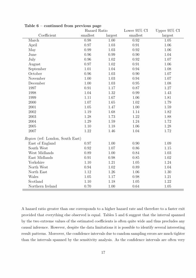
Table 6 – continued from previous pageHazard Ratio Lower 95% CI Upper 95% CI
Coefficient smallest largest smallest largestMarch 0.98 1.00 0.92 1.05April 0.97 1.03 0.91 1.06May 0.99 1.03 0.92 1.06June 0.96 0.99 0.90 1.04July 0.96 1.02 0.92 1.07August 0.97 1.02 0.91 1.06September 1.01 1.04 0.94 1.08October 0.96 1.03 0.90 1.07November 1.00 1.03 0.94 1.07December 1.00 1.03 0.95 1.081997 0.91 1.17 0.87 1.271998 1.04 1.32 0.99 1.431999 1.11 1.67 1.06 1.812000 1.07 1.65 1.02 1.792001 1.05 1.47 1.00 1.592002 1.19 1.68 1.14 1.822003 1.28 1.73 1.22 1.882004 1.29 1.59 1.24 1.722005 1.10 1.18 1.06 1.282007 1.22 1.46 1.04 1.72
Region (ref: London, South East)East of England 0.97 1.00 0.90 1.09South West 0.92 1.07 0.86 1.15West Midlands 0.89 1.00 0.84 1.03East Midlands 0.91 0.98 0.85 1.02Yorkshire 1.10 1.21 1.05 1.24North West 0.94 1.02 0.89 1.04North East 1.12 1.26 1.06 1.30Wales 1.05 1.17 0.98 1.21Scotland 1.10 1.18 1.05 1.22Northern Ireland 0.70 1.00 0.64 1.05
A hazard ratio greater than one corresponds to a higher hazard rate and therefore to a faster exit
provided that everything else observed is equal. Tables 5 and 6 suggest that the interval spanned
by the two extreme values of the estimated coefficients is often quite wide and thus precludes any
causal inference. However, despite the data limitations it is possible to identify several interesting
result patterns. Moreover, the confidence intervals due to random sampling errors are much tighter
than the intervals spanned by the sensitivity analysis. As the confidence intervals are often very
17

tight (almost zero), we do not perform statistical tests for equality of coefficients. We will now
look at the estimation results in more detail.
Socio Demographics The results suggest that older unemployed have longer unemployment
periods before they find employment and it takes longer until they start a training measure.
Further nonparametric evidence using the estimator of Wichert and Wilke (2008) suggests that
conditional quantile functions are almost constant in age for up to the 0.7 quantile. The age coef-
ficient of the Cox model seems to be mainly driven by longer long-term unemployment of females.
Younger unemployed start a training measure quicker, while there is no conclusive evidence for a
faster start of employment. Singles are slower in starting employment while single females start
training much faster.
Occupation There are reversed result patterns for failure type of employment and ALMP. While
less skilled are slower in starting a job, they are faster in starting a training measure. The contrary
applies to individuals in senior or professional positions. Surprisingly, the reference group with
unknown occupation is closest to the senior professional group. This indicates that the group of
individuals who do not report their occupation is a positive selection as it is unlikely that the
majority of them is at the senior level.
Work History A pre-existing unemployment period is not clearly associated with a longer
current unemployment period prior to starting a new job. There is, however, strong evidence
that the assignment into training is much quicker in case of repeated unemployment. Looking
at additional coefficients derived from past or previous unemployment spells, further strong re-
sult patterns emerge: if the unemployed was already in ALMP in the past, this is associated
with a slower job finding rate and a quicker assignment into another training measure. Thus,
the data gives evidence for labour market measures careers which are characterised by repeated
participation in training measures and low employment probabilities. If the unemployed entered
employment at the end of her/his last unemployment period, this shortens unemployment until
job finding while it drastically decreases the assignment speed into ALMP. This suggests that
mainly unemployed with weak labour market performance are assigned to labour market pro-
grammes. The same result patterns are also observed in the German labour market with much
more comprehensive data (Arntz and Wilke, 2008).
Calender Time Results regarding the calender time are robust. There is almost no evidence for
seasonal unemployment patterns in the UK, except of the months of September-November. The
seasonality in these months may be attributed to tourism or agriculture. Firms in these business
18

sectors usually decrease their workforce during the winter period. In terms of calender years there
are shorter unemployment periods in 1999-2004 and a considerable prolongation from 2004 to
2007. This is maybe some evidence for a general downtourning of the British labour market. The
assignment into ALMP was faster following the introduction of the new deal programme at the
end of 1998. This is well reflected by the data.
Region The result patterns for regional variation are also quite robust. Unemployed in the
South East, London, the West Midlands and Northern Ireland have the longest duration until
finding a new job, while it is shortest in the South West. The assignment into ALMP is fastest in
Yorkshire, the North East and Scotland.
It is difficult to compare these results to results of the other studies by Kalwij (2004) and
McVicar and Podivinsky (2002, 2003) as these papers use different methods and observation
periods. In addition, McVicar and Podivinsky use data for the 18-24 years old only. Kalwij
(2004) does not include observed individual specific variables apart from calender time and regional
information. A considerable share of his coefficients does not fall into the intervals of this paper. It
is unclear whether this is due to the econometric model, the observation period or due to different
data preparation.
5 Summary and Conclusion
This paper explores the implications of missing information in UK administrative spell data for
unemployment duration analysis. The main points of the paper can be summarised as follows:
• As the information in the JUVOS is restricted to claim periods, empirical research is limited
as the data does not fully identify unemployment duration. In many cases the actual start-
and endpoint are unknown. Moreover, the pre- and post-unemployment labour market state
of the unemployed are often unknown.
• These limitations are tackled as follows: based on some plausible criteria, we constructed
unemployment duration by merging two or several subsequent claim periods and any unob-
served gaps. Also, the uncertainty about the start date of the unemployment duration was
reduced by restricting the analysis to unemployment spells with a pre-existing employment
spell only.
• Our empirical analysis suggests that the data preparation steps have a strong influence on
the resulting statistics. This highlights that the information content of the JUVOS may be
19

rather limited for the specific purpose of the analysis. Empirical researchers should therefore
undertake a sensitivity analysis or adapt their statistical model to account for the data issues.
The results also suggest that there are robust result patterns. Therefore, the JUVOS can
be a stable data source for applied research but it depends on the specific research question
at hand.
• Due to the large sample size of the data, random sampling errors are of minor importance.
To validate the stable empirical result patterns of this paper, further research could analyse their
robustness with respect to the choice of the econometric model. It would also be interesting to
investigate the robustness of previous work based on the JUVOS.
Depending on the research question at hand, the JUVOS may not contain enough information
to identify sharp result pattern. In this case, an alternative data set such as survey data could
contribute valuable identifying information. However, survey data has other limitations such as a
limited sample size which does not allow an analysis of subgroups such as young or old unemployed.
The availability of merged administrative data from the United Kingdom under well defined access
requirements by the data suppliers would be therefore an important contribution to improve the
quality of independent research under equal opportunities.
References
[1] Arntz, M. and Wilke, R.A. (2008), Unemployment duration in Germany: individual and re-
gional determinants of local job finding, migration and subsidized employment, Regional Studies,
forthcoming.
[2] Arntz, M., Lo, S. and Wilke, R.A. (2007) Bounds analysis of competing risks: a nonparametric
evaluation of the effect of unemployment benefits on migration in Germany. ZEW Discussion
Paper No. 07-049. ZEW, Mannheim.
[3] Blundell, R., Costa Dias, M., Meghir, C. and van Reenen, J. (2004) Evaluating the Em-
ployment Impact of mandatory a job search assistance programmem. Journal of the European
Economics Association, 2, 569–606.
[4] Bryson, A. and Kasparova, D. (2003) Profiling benefits claimants in Britain: A feasibility
study. DWP Research Report No. 196, DWP, London.
[5] Card, D., Chetty, R. and Weber, A. (2007) The spike at benefit exhaustion: leaving the
unemployment system or starting a new job? American Economic Review, 97, 113–118.
20
[6] Dolton, P. and O’Neill, D. (2002) The long-run effects of unemployment monitoring and work-
search programs: experimental evidence from the United Kingdom. Journal of Labour Eco-
nomics, 20, 381–403.
[7] DWP (2008) New policy inititatives: expectations and evidence, presented at the WPEG
conference 2008, Sheffield.
[8] Cox, D.R. (1972) Regression model and life tables. Journal of the Royal Statistical Society B,
34, 187-220.
[9] Fitzenberger, B. and Wilke, R.A. (2004), Unemployment Durations in West-Germany Before
and After the Reform of the Unemployment Compensation System During the 1980s, ZEW
Discussion Paper No. 04-24. ZEW, Mannheim.
[10] Green, H., Marsh, A., Connolly, H. and Payne, J. (2003) Final Effects of ONE: Part one,
DWP Research Report No. 183, DWP, London.
[11] Kalwij, S. (2004) Unemployment experiences of young men: on the road to stable employ-
ment? Oxford Bulletin of Economics and Statistics, 66, 205–237.
[12] Kaplan, E. L., and Meier, P. (1958) Nonparametric estimation from incomplete observations.
Journal of the American Statistical Association, 53, 457–481.
[13] Kruppe, T., Muller, E., Wichert, L. and Wilke, R.A. (2008) On the definition of unemploy-
ment and its implementation in register data - the case of Germany. Schmollers Jahrbuch, 128,
forthcoming.
[14] Kossigh, J., Walker, I. and Zhu, Y. (2008) Getting dads to pay and keeping mums at work:
the conflicting effects of a child support disregarded, presented at the WPEG conference 2008,
Sheffield.
[15] Lee, S. and Wilke, R.A. (2008). Reform of unemployment compensation in Germany: A
nonparametric bounds analysis using register data. Journal of Business and Economic Statistics,
forthcoming.
[16] Ludemann, E., Wilke, R.A. and Zhang, X. (2006) Censored Quantile Regression and the
Length of Unemployment Periods in West-Germany. Empirical Economics, 31, 1003–1024.
[17] Machin, A. (2004) Comparison between unemployment and the claimant count. Labour Mar-
ket Trends, February 2004, 59–62
21

[18] Machin, S. and Manning, A. (1999) The Causes and Consequences of Long-term Unemploy-
ment in Europe. in: Handbook of Labor Economics. Vol. 3C, edited by Ashenfelter, O.; Card,
D., North-Holland.
[19] Manning, A. (2005) You can’t always get what you want: The impact of the UK Jobseeker’s
allowance. CEP Discussion Paper No. 697, Centre for Economic Performance, London.
[20] Manski, C.F. (2003), Partial Identification of Probability Distributions, New York.
[21] McVicar, D. and Podivinsky, J. (2002) Unemployment duration before and after the new
deal. NIERC Working Paper Series No.74., Belfast.
[22] McVicar, D. and Podivinsky, J. (2003) How well has the new deal for young people worked
in the UK regions? NIERC Working Paper Series No.79., Belfast.
[23] National Statistics (2007) How exactly is unemployment measured?
http://www.statistics.gov.uk/statbase/Product.asp?vlnk=2054
[24] Van den Berg, G.J. and Van Ours, J.C. (1994) Unemployment dynamics and duration depen-
dence in France, the Netherlends and the United Kingdom. Economic Journal, 104, 432–443.
[25] Ward, H. and Bird, D. (1995) The Juvos Cohort: A longitudinal database of the claimant
unemployed. Employment Gazette, September, 345–350.
[26] Wichert, L. and Wilke, R.A. (2008) Simple non-parametric estimators for unemployment
duration analysis Journal of the Royal Statistical Society: Series C, 57, 117-126.
[27] Wolstenholme, S. (2004) Destination of benefit leavers 2004, Re-
search Summary of the Department for Work and Pensions, London
http://www.bmrb.co.uk/content/Files/DWP%20Report.pdf .
22

Appendix
Table 7: Descriptive Statistics for the samples used inthe Cox regressions
transition fromany state employment
variable Concept 1 Concept 5 Concept 1 Concept 5Socio Demographics
< 26 years old 0.40 0.44 0.34 0.34> 55 years old 0.05 0.05 0.05 0.06single 0.70 0.71 0.72 0.71female 0.29 0.31 0.24 0.24single*female 0.20 0.21 0.17 0.17
Occupation (ref: unknown)elementary 0.28 0.28 0.30 0.30manufacturing 0.06 0.06 0.08 0.08trade, services 0.36 0.37 0.37 0.37technical 0.05 0.04 0.04 0.04senior, professional 0.08 0.07 0.08 0.08
Work Historypast unemployment 0.80 0.64 1.00 1.00past incapacity benefits 0.05 0.03 0.05 0.04past income support 0.02 0.01 0.01 0.01past ALMP 0.20 0.25 0.15 0.16prev. employment 0.34 0.55 1.00 1.00prev. mobility 0.27 0.22 0.26 0.35
Calender Time (ref: January 2006)February 0.08 0.08 0.08 0.08March 0.09 0.08 0.09 0.09April 0.08 0.08 0.08 0.08May 0.08 0.07 0.07 0.07June 0.09 0.08 0.08 0.08July 0.08 0.09 0.08 0.08August 0.08 0.08 0.07 0.07September 0.08 0.08 0.08 0.08October 0.08 0.08 0.09 0.09November 0.08 0.08 0.09 0.09December 0.07 0.08 0.09 0.091997 0.12 0.10 0.10 0.101998 0.11 0.11 0.11 0.111999 0.11 0.11 0.11 0.112000 0.10 0.10 0.11 0.11
Continued on next page
23
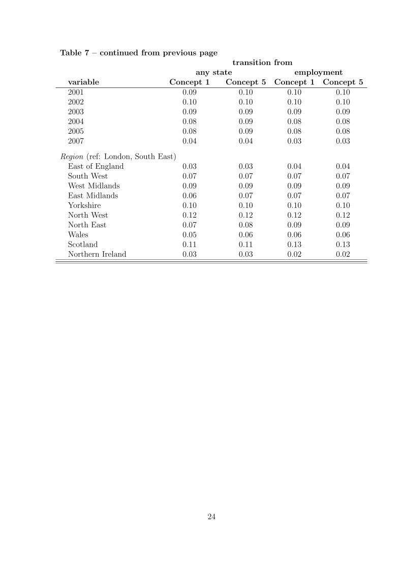
Table 7 – continued from previous pagetransition from
any state employmentvariable Concept 1 Concept 5 Concept 1 Concept 52001 0.09 0.10 0.10 0.102002 0.10 0.10 0.10 0.102003 0.09 0.09 0.09 0.092004 0.08 0.09 0.08 0.082005 0.08 0.09 0.08 0.082007 0.04 0.04 0.03 0.03
Region (ref: London, South East)East of England 0.03 0.03 0.04 0.04South West 0.07 0.07 0.07 0.07West Midlands 0.09 0.09 0.09 0.09East Midlands 0.06 0.07 0.07 0.07Yorkshire 0.10 0.10 0.10 0.10North West 0.12 0.12 0.12 0.12North East 0.07 0.08 0.09 0.09Wales 0.05 0.06 0.06 0.06Scotland 0.11 0.11 0.13 0.13Northern Ireland 0.03 0.03 0.02 0.02
24
Related Documents