Understanding Physiological and Degenerative Natural Vision Mechanisms to Define Contrast and Contour Operators

Understanding Physiological and Degenerative NaturalVision Mechanisms to Define Contrast and ContourOperatorsJacques Demongeot*, Yannick Fouquet, Muhammad Tayyab, Nicolas Vuillerme

TIMC-IMAG, UMR UJF/CNRS 5525, University J. Fourier of Grenoble, La Tronche, France

Abstract

Background: Dynamical systems like neural networks based on lateral inhibition have a large field of applications in imageprocessing, robotics and morphogenesis modeling. In this paper, we will propose some examples of dynamical flows usedin image contrasting and contouring.

Methodology: First we present the physiological basis of the retina function by showing the role of the lateral inhibition inthe optical illusions and pathologic processes generation. Then, based on these biological considerations about the realvision mechanisms, we study an enhancement method for contrasting medical images, using either a discrete neuralnetwork approach, or its continuous version, i.e. a non-isotropic diffusion reaction partial differential system. Following this,we introduce other continuous operators based on similar biomimetic approaches: a chemotactic contrasting method, aviability contouring algorithm and an attentional focus operator. Then, we introduce the new notion of mixed potentialHamiltonian flows; we compare it with the watershed method and we use it for contouring.

Conclusions: We conclude by showing the utility of these biomimetic methods with some examples of application inmedical imaging and computed assisted surgery.

Citation: Demongeot J, Fouquet Y, Tayyab M, Vuillerme N (2009) Understanding Physiological and Degenerative Natural Vision Mechanisms to Define Contrastand Contour Operators. PLoS ONE 4(6): e6010. doi:10.1371/journal.pone.0006010

Editor: Ernest Greene, University of Southern California, United States of America

Received August 29, 2008; Accepted February 21, 2009; Published June 23, 2009

Copyright: � 2009 Demongeot et al. This is an open-access article distributed under the terms of the Creative Commons Attribution License, which permitsunrestricted use, distribution, and reproduction in any medium, provided the original author and source are credited.

Funding: This work has been supported by the EC project Alfa IPECA and by the EC NoE VPH. The funders had no role in study design, data collection andanalysis, decision to publish, or preparation of the manuscript.

Competing Interests: The authors have declared that no competing interests exist.

* E-mail: [email protected]

Introduction

‘‘In nova fert animus mutatas dicere formas corpora…’’ I want to speak about

bodies changed into new forms… (Ovid, Metamorphoses, Book 1st, 10 AD).

In the vertebrate retina, cones are hyperpolarized when

illuminated by light, but also receive a depolarizing input when

receptors some distance away are illuminated. This antagonistic

center-surround response is mediated by amacrine and horizontal

cells (Figure 1), through a sign-reversing synapse to the cones often

called feedback synapse, the global mechanism being called lateral

inhibition [1–3]. This surround response is involved in edge

enhancement and image contrasting [4–16] realizing concretely

the Mach (boundary brightness overshoot) and the Marr

(Laplacian zero-crossing edge-enhancement) effects, used in many

image processing applications [17]. A number of contrast illusions

(Figures 2, 3, 4) have been described [18] based on the lateral

inhibition principle. In order to examine how rod and cone

functions are differentially affected during retinal degeneration

(abolishing the contrast), many studies have been done on the

genetic level showing that these two cell types have complemen-

tary roles during both development and degenerative processes

[19–21]. For understanding the retinal physiology as well as this

pathology, many models [22–34] are now available which try to

mimic relevant adaptation behaviours of the human visual system,

like lightness/colour constancy and contrast enhancement,

corresponding to the ability of the visual system to increase the

appearance of large-scale light-dark or inter-colour transitions,

similar to how sharpening with an ‘‘un-sharp mask’’ increases the

appearance of small-scale edges.

These models use theoretical developments [35–44] in dynam-

ical systems, especially the study of their attractors. An attractor

represents the ultimate evolution of a dynamical system when time

tends to infinity; after perturbations, an attractor recovers its stable

dynamical features, like its period and amplitude. That requires a

rigorous mathematical framework for defining the continuous flow

and its convergence speed to attractors, and after its discrete

version, i.e. an iteration process representing the succession of

states of the dynamical system. These theoretical advances have

permitted the development of fast image processing algorithms

used in rapid contrasting methods [45–58] implemented in real-

time processors [59–68], and the development of contouring

methods like snakes, snake-splines, d-snakes, which allow a global

definition of the boundaries of objects of interest in an image.

These algorithms have emphasized the role played by computer

implemented procedures, starting from an initial compact, e.g. a

sphere, and ending at the final shape of the object’s contours after

a certain number of iterations [69–80]. The corresponding flow is

a compact set valued flow, the simplest deriving from a potential

PLoS ONE | www.plosone.org 1 June 2009 | Volume 4 | Issue 6 | e6010

[81–86]. In general, this methodology allows one to rapidly and

automatically obtain 3D contours, which is necessary in medical

imaging to perform computer aided medical interventions. If the

dynamics are conservative in a neighbourhood of an attractor, the

flow becomes Hamiltonian, so we then will define the notion of

mixed potential Hamiltonian flow. This flow gives a theoretical

support to the Waddington’s notion of chreod, particularly

relevant in embryonic morphogenesis modeling [87–91], but also

serves in image contouring.

Using the previously introduced theoretical notions, we study an

enhancement method for contrasting medical images, using either

a discrete neural network approach, or its continuous version, i.e. a

reaction-diffusion partial differential system [92–99]. Indeed,

having the goal of providing for a rapid and efficient action

[100–142] in precise surgical robotics as well as in disease

diagnosis and satellite control imaging, such pre-treatments are

performed for contrasting and then contouring images. The

medical community, for example, often uses pre-treated

anatomical images coming from imaging devices, like MRI or

CT-scanner, whose pre- processing involves two fundamental

steps: contrasting and contouring. The natural vision executes

these two tasks, the first one being based on the architecture of

the retina, which uses lateral inhibition to reinforce the

perception of the contours of homogeneous objects in a scene.

Because the objects of medical interest are homogeneous with

respect to their environment (a tumour or an organ are made

of cells coming from the same cellular clone), they are well

enhanced by using operators processing as in the natural vision.

Therefore, we introduce continuous operators generalizing

discrete neuromimetic approaches using lateral inhibition as

well as analogs of the Hebbian rule for the evolution of synaptic

weights.

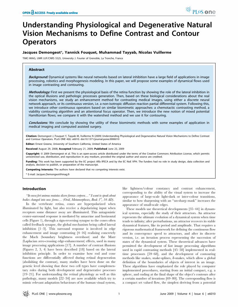
Figure 1. Physiological and pathological retina. Top left: lateral inhibition due to horizontal cell synapses [after 3]. Top right: confocalmicroscopy slice of mouse retina with retinitis pigmentosa coming from T. Leveillard & J.A. Sahel [19]. Bottom left: segmentation of cones and rodswith a cell deficit in the quadrant Left Superior (LS) [34]. Bottom right: histogram of the intercept distances showing an augmentation of the inter-celldistance in the quadrant Left Superior with respect to others Left Inferior (LI), Right Superior and Inferior (RS & RI) [34].doi:10.1371/journal.pone.0006010.g001

Contrast and Contour Operators


Results

The results presented in this Section involve consecutive phases

of contrasting and segmenting in order to identify objects of

interest in an image. The important features of a scene are the

prey, predators, and sexual partners. For the detection of these

features, the major characteristics are the ‘‘phaneres’’, this word

coming from the Greek phaneros: visible. The ‘‘phaneres’’ in

animals and plants are prominent visible tegumentary formations

like feathers, scales, hair, petals, skin spots and stripes of various

forms and colours. The role of the contrasting pre-treatment in the

retina is to rapidly enhance the characteristics (luminance, colour

and texture) on the boundaries of the homogeneous zones in a

scene in order to improve their perception and extract the features

associated to the vital functions like the nutrition, the survival and

the reproduction. This process can trigger very fast actions (like

escaping a predator) after a stimulus of about 150 ms [136]. Such

fast sensory-motor loops need a very simple and rapid mechanism

well encoded in the anatomy and in the physiology of the retina

(like the center-surround response of cones and rods [1–3]), early

before a semantic recognition and denomination of the prey or of

the predator. We will give first some results concerning the natural

contrasting process both in a natural and in a simulation context.

Pathologic retinaThe lateral inhibition mechanism in the retina is due to the

presence of feedback synapses of horizontal cells [1,2], which

reverse the sign from activation of the cells surrounding that were

illuminated (Figure 1 top left). The retina pathologies provoke a

progressive death of rods (as in retinitis pigmentosa) followed by

the apoptosis of the cones; then, the non-secretion by rods of a

growth factor favouring the cones survival, causes the disappear-

ance of the lateral inhibition, hence of the contrasting ability

[4,19,20,21]. As shown in the top right and bottom left of Figure 1

on a confocal slice of a sick retina, we observe an important loss of

both rods and cones in the left superior quadrant. An analysis of

interdistances among cells in the three other quadrants shows that

the mean interdistance between cones in the peripheral retina

(about 20 m) is better conserved than the corresponding value

between rods (about 3 m), proving the primary rod degeneracy.

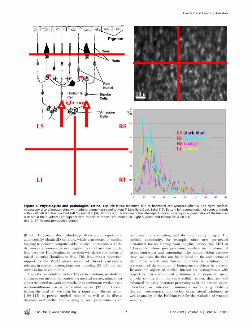
Contrast illusionsThe perception of artefactual stripes or spots comes from the

lateral inhibition effect, which causes a reinforcement (respectively

decline) of brightness in a pixel if its neighbours are black

(respectively white). This illusion effect is visible on the Figures 2 to

4. In Figure 2 (top-left), the Hermann illusion is provoked by the

local organization of inhibition and activation between retinal

cells, which is described bottom right. The illusion shows bright

squares at the intersection of grey stripes and grey squares at the

intersection of white stripes. In Figure 2 (bottom-left), the Mach

bands illusion gives an enhancement of the vertical lines separating

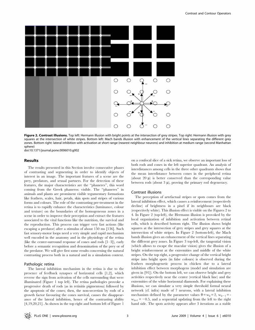
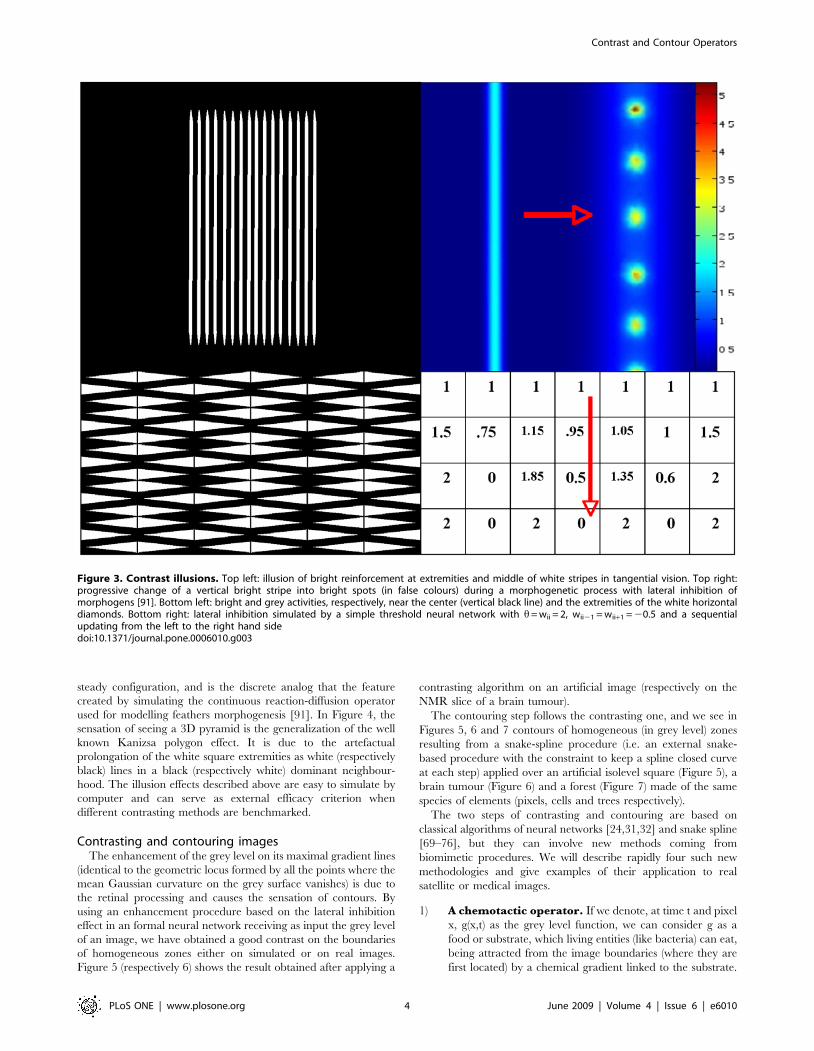
the different grey zones. In Figure 3 top-left, the tangential vision

(which allows to escape the macular vision) gives the illusion of a

bright reinforcement at the extremities and middle of the white

stripes. On the top right, a progressive change of the vertical bright

stripe into bright spots (in false colours) is observed during the

feathers morphogenetic process in chicken due to a lateral

inhibition effect between morphogens (model and simulation are

given in [91]). On the bottom left, we can observe bright and grey

activities respectively near the center (vertical black line) and the

extremities of the white horizontal diamonds. For explaining these

illusions, we can simulate a very simple threshold formal neural

network (cf. infra) made of 7 neurons, with a lateral inhibition

mechanism defined by the parameter values h= wii = 2, wii21 = -

wii+1 = 20.5, and a sequential updating from the left to the right

hand side. The spots activity appears after 3 iterations as a stable

Figure 2. Contrast illusions. Top left: Hermann illusion with bright points at the intersection of grey stripes. Top right: Hermann illusion with greysquares at the intersection of white stripes. Bottom left: Mach bands illusion with enhancement of the vertical lines separating the different greyzones. Bottom right: lateral inhibition with activation at short range (nearest neighbour neurons) and inhibition at medium range (second Manhattansphere)doi:10.1371/journal.pone.0006010.g002



steady configuration, and is the discrete analog that the feature

created by simulating the continuous reaction-diffusion operator

used for modelling feathers morphogenesis [91]. In Figure 4, the

sensation of seeing a 3D pyramid is the generalization of the well

known Kanizsa polygon effect. It is due to the artefactual

prolongation of the white square extremities as white (respectively

black) lines in a black (respectively white) dominant neighbour-

hood. The illusion effects described above are easy to simulate by

computer and can serve as external efficacy criterion when

different contrasting methods are benchmarked.

Contrasting and contouring imagesThe enhancement of the grey level on its maximal gradient lines

(identical to the geometric locus formed by all the points where the

mean Gaussian curvature on the grey surface vanishes) is due to

the retinal processing and causes the sensation of contours. By

using an enhancement procedure based on the lateral inhibition

effect in an formal neural network receiving as input the grey level

of an image, we have obtained a good contrast on the boundaries

of homogeneous zones either on simulated or on real images.

Figure 5 (respectively 6) shows the result obtained after applying a

contrasting algorithm on an artificial image (respectively on the

NMR slice of a brain tumour).

The contouring step follows the contrasting one, and we see in

Figures 5, 6 and 7 contours of homogeneous (in grey level) zones

resulting from a snake-spline procedure (i.e. an external snake-

based procedure with the constraint to keep a spline closed curve

at each step) applied over an artificial isolevel square (Figure 5), a

brain tumour (Figure 6) and a forest (Figure 7) made of the same

species of elements (pixels, cells and trees respectively).

The two steps of contrasting and contouring are based on

classical algorithms of neural networks [24,31,32] and snake spline

[69–76], but they can involve new methods coming from

biomimetic procedures. We will describe rapidly four such new

methodologies and give examples of their application to real

satellite or medical images.

1) A chemotactic operator. If we denote, at time t and pixel

x, g(x,t) as the grey level function, we can consider g as a

food or substrate, which living entities (like bacteria) can eat,

being attracted from the image boundaries (where they are

first located) by a chemical gradient linked to the substrate.

Figure 3. Contrast illusions. Top left: illusion of bright reinforcement at extremities and middle of white stripes in tangential vision. Top right:progressive change of a vertical bright stripe into bright spots (in false colours) during a morphogenetic process with lateral inhibition ofmorphogens [91]. Bottom left: bright and grey activities, respectively, near the center (vertical black line) and the extremities of the white horizontaldiamonds. Bottom right: lateral inhibition simulated by a simple threshold neural network with h= wii = 2, wii21 = wii+1 = 20.5 and a sequentialupdating from the left to the right hand sidedoi:10.1371/journal.pone.0006010.g003



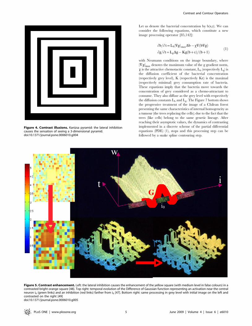
Let us denote the bacterial concentration by b(x,t). We can

consider the following equations, which constitute a new

image processing operator [85,142]:

Lb=L t~Lb +gj jmaxDb{x+ b+gð Þ

Lg=Lt~LgDg{Kg bzeð Þ= bz1ð Þð1Þ

with Neumann conditions on the image boundary, where

+gj jmax denotes the maximum value of the g gradient norm,

x is the attractive chemotactic constant, Lb (respectively Lg) is

the diffusion coefficient of the bacterial concentration

(respectively grey level), K (respectively Ke) is the maximal

(respectively minimal) grey consumption rate of bacteria.

These equations imply that the bacteria move towards the

concentration of grey considered as a chemo-attractant to

consume. They also diffuse as the grey level with respectively

the diffusion constants Lb and Lg. The Figure 7 bottom shows

the progressive treatment of the image of a Chilean forest

presenting the same characteristics of internal homogeneity as

a tumour (the trees replacing the cells); due to the fact that the

trees (like cells) belong to the same genetic lineage. After

reaching their asymptotic values, the dynamics of contrasting

implemented in a discrete scheme of the partial differential

equations (PDE) (1), stops and this processing step can be

followed by a snake spline contouring step.

Figure 4. Contrast illusions. Kanizsa pyramid: the lateral inhibitioncauses the sensation of seeing a 3-dimensional pyramid.doi:10.1371/journal.pone.0006010.g004

Figure 5. Contrast enhancement. Left: the lateral inhibition causes the enhancement of the yellow square (with medium level in false colours) in acontrasted bright orange square [48]. Top right: temporal evolution of the Difference of Gaussian function representing an activation near the centralneuron i0 (green links) and an inhibition (red links) farther from i0 [47]. Bottom right: same processing in grey level with initial image on the left andcontrasted on the right [49]doi:10.1371/journal.pone.0006010.g005



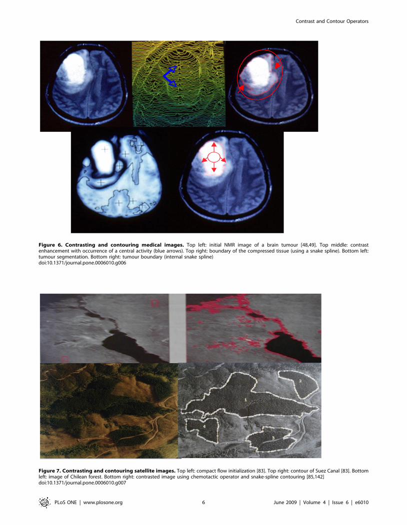
Figure 6. Contrasting and contouring medical images. Top left: initial NMR image of a brain tumour [48,49]. Top middle: contrastenhancement with occurrence of a central activity (blue arrows). Top right: boundary of the compressed tissue (using a snake spline). Bottom left:tumour segmentation. Bottom right: tumour boundary (internal snake spline)doi:10.1371/journal.pone.0006010.g006

Figure 7. Contrasting and contouring satellite images. Top left: compact flow initialization [83]. Top right: contour of Suez Canal [83]. Bottomleft: image of Chilean forest. Bottom right: contrasted image using chemotactic operator and snake-spline contouring [85,142]doi:10.1371/journal.pone.0006010.g007



2) A viability contouring operator. If we minimize the

following function,

aS K tð Þð ÞzbV K tð Þð Þzc

ðLK tð Þ

1= +g xð Þk k½ � dx ð2Þ

we obtain a new snake operator [75,85], where K(t) is a

compact object of interest moving toward a limit set K(‘),

whose external surface S as well as its inner volume V are

minimized, allowing a contouring with real gloves (precise

contour) contrarily to mittens (convex envelop) often observed

with the Mumford-Kass-Terzopoulos algorithm in Figure 7

[69,70]. We see in Figure 7 (top and bottom right) the

contouring done by imposing a bicubic spline to the boundary

at each time step [71,72], followed by a 3D spline smoothing.

Many other approaches can also be used for controlling the

active-shape models. This is the case in the level set methods

used for computing and analyzing the motion of an interface

in two or three dimensions by modelling the velocity vector

field through Euler-Lagrange or Hamilton-Jacobi PDE’s

[77,78,79,80]. These PDE’s can be used to model the

segmentation of a moving 3D object (like the heart) giving a

particular status to the pixels having a maximal velocity or

acceleration of their grey levels. This procedure has been used

for segmenting the pericardium [131].

3) A non-isotropic reaction-diffusion operator. If we

consider the grey level function g(x,0) as the initial image, we

can follow the transient behaviour of the non-linear diffusion

operator defined in [93]:

Lg=L t~ Ldiv 1 0,s½ � +(G � gj j:+g� ��

ð3Þ

Here G is a Gaussian kernel of fixed variance and with

Neumann conditions. Its asymptotes correspond to a

constant grey level suppressing the objects of interest inside

the image. For that reason, we consider now a non-isotropic

reaction-diffusion operator defined in [93,95,96]:

Lg=Lt{div L+gð Þ~0,dL=dtzL=t~s2P+g=t, if +gjj ws

~ +gjj 2P+gz3 s2{ +gjj 2

� �Id=2, if +gjj ƒs

ð4Þ

where L is a 262 matrix and P=g is the orthogonal

projection matrix:

P+g~1= +gjj 2 Lg=Lxð Þ2 - Lg=Lxð Þ Lg=Lyð Þ- Lg=Lyð Þ Lg=Lxð Þ Lg=Lxð Þ2

!ð5Þ

In the equations above, the diffusion constant L becomes

variable with the time t and its evolution equation is similar

to the Hebbian rule of a discrete neural network operator.

Treated images are obtained at the asymptotic state of the

PDE dynamics as for neural networks [48,49] with lateral

inhibition (Figure 6). A comparison done in [96] shows that

the asymptotes of this non-isotropic operator are better than

for some of the operators described earlier. More generally,

we can notice in the other PDE approaches:

a) The application of the pure heat operator [145] quickly leads

to a constant grey level

b) In the Perona-Malik operator [92], the viscosity is different

within a region and across its boundary in order to encourage

smoothing inside the region of interest; this operator can be

used transiently for this purpose before the non-isotropic

reaction-diffusion operator

c) The Catte-Lions-Morel-Coll algorithm [94] gives a good

contrasting during the transient behaviour of the operator,

but has the same asymptotes as for the pure heat algorithm

(even it is reached more slowly)

d) The non-isotropic reaction-diffusion operator [93,95,96]

offers a reasonable asymptotic processing

e) The Weickert operator [97] permits the completion of

interrupted lines or the enhancement of flow-like structures

by choosing the appropriate smoothing direction in aniso-

tropic processes in spirit to the Cottet–Germain filter [95]

f) The Tschumperle-Deriche operator [98,99] allows the

regularization of velocity vectors fields in 4D imaging

(acquired for example during the motion of a 3D camera).

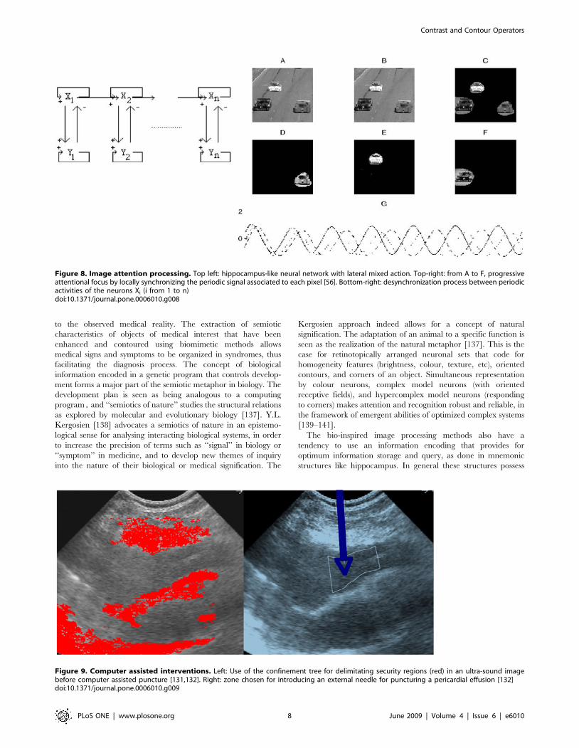
4) An attentional focus operator. For focusing on only one

region of interest, we have to change the image input on an

artificial neural network [56]. This input can be constant

[24,31,32], stochastic [47–54] or deterministic periodic [56].

This last coding mimics the information storage inside the

hippocampus in which the functional unit, made of two

neurons in mixed inhibition/activation interaction (Figure 8

top left) has an attractor limit cycle. We can locally

synchronize, using an evocation stimulus, and desynchro-

nize, by introducing noise on the inter-unit interactions, the

periodic activities corresponding to initially non phase-

locked neurons. In this way, we enhance considerably (by

forcing the units to add their maximal activities at the same

time) the grey level on the zones of local synchronization

(Figure 8 E bottom right). Then, by thresholding and

segmenting, we get the parts of the initial image (Figure 8 A

top right) on which the attentional focus has been exerted

(Figure 8D, E, F top right).

Computer assisted interventionsFor introducing and driving medical or surgical tools (like

needles, electrodes, bistouries) into the human body [118–135],

one needs to segment and contour (after contrasting) zones of

interest to avoid (as indicated by red zones in Figure 9 left

representing tissues of lungs on the top and cardiac muscle on the

middle and bottom) or to reach (blue arrow in Figure 9 right

indicating a pericardial effusion). This example gives a good

illustration of what can be exploited from the contrasting and

contouring operators in order to go farther than the descriptive

level for diagnosis. That is to really improve some medical

procedures, one must automate the process completely, thus

replacing the human actor without any loss of speed or precision

[119–130].

Discussion

Interest of the biomimetic approachThe biomimetic approach used in numerous methods presented

in this paper, especially for the contrasting phase, exploits the

efficiency of visual data processing procedures that have been

selected by natural evolution. These procedures represent an

optimum in terms of economy of implementation (small number of

living elements involved, like cells, tissues, vessels, etc), speed and

precision. They also are based on operations that come after

processing by the retina and visual areas, thus providing high level

semantic neural networks that define the symptomatology related



to the observed medical reality. The extraction of semiotic

characteristics of objects of medical interest that have been

enhanced and contoured using biomimetic methods allows

medical signs and symptoms to be organized in syndromes, thus

facilitating the diagnosis process. The concept of biological

information encoded in a genetic program that controls develop-

ment forms a major part of the semiotic metaphor in biology. The

development plan is seen as being analogous to a computing

program, and ‘‘semiotics of nature’’ studies the structural relations

as explored by molecular and evolutionary biology [137]. Y.L.

Kergosien [138] advocates a semiotics of nature in an epistemo-

logical sense for analysing interacting biological systems, in order

to increase the precision of terms such as ‘‘signal’’ in biology or

‘‘symptom’’ in medicine, and to develop new themes of inquiry

into the nature of their biological or medical signification. The

Kergosien approach indeed allows for a concept of natural

signification. The adaptation of an animal to a specific function is

seen as the realization of the natural metaphor [137]. This is the

case for retinotopically arranged neuronal sets that code for

homogeneity features (brightness, colour, texture, etc), oriented

contours, and corners of an object. Simultaneous representation

by colour neurons, complex model neurons (with oriented

receptive fields), and hypercomplex model neurons (responding

to corners) makes attention and recognition robust and reliable, in

the framework of emergent abilities of optimized complex systems

[139–141].

The bio-inspired image processing methods also have a

tendency to use an information encoding that provides for

optimum information storage and query, as done in mnemonic

structures like hippocampus. In general these structures possess

Figure 8. Image attention processing. Top left: hippocampus-like neural network with lateral mixed action. Top-right: from A to F, progressiveattentional focus by locally synchronizing the periodic signal associated to each pixel [56]. Bottom-right: desynchronization process between periodicactivities of the neurons Xi (i from 1 to n)doi:10.1371/journal.pone.0006010.g008

Figure 9. Computer assisted interventions. Left: Use of the confinement tree for delimitating security regions (red) in an ultra-sound imagebefore computer assisted puncture [131,132]. Right: zone chosen for introducing an external needle for puncturing a pericardial effusion [132]doi:10.1371/journal.pone.0006010.g009



their own formats of information encoded in periodic temporal

neuronal activities that we can mimic to optimize both

compression and retrieving procedures [40]. All these neural

treatments can induce illusions and artefacts. But the knowledge

about their origin can be used for preventing such abnormalities in

the low level (contrasting and contouring) as well as in the high

level (semantic assignation and recognition) image processing

steps. The neural treatments need also to avoid pathologic

processing, due to a non-optimal number of their neurons and/

or interactions and to a non robust value of their parameters. To

that precise purpose, a deep scientific knowledge about the

physiology and the pathology of the retina constitutes an

unavoidable inheritance.

Limits of the biomimetic approachIn order to be faster, the methods mimicking the natural

process of vision need to be made parallel as in the real neuronal

systems. But the attractors of the dynamical systems permitting

contrasting and contouring of the images are highly dependent

on their modality of implementation, particularly on their

updating mode. In general, the fixed configurations obtained

by simulating such systems are robust with respect to the mode

of updating, but it is not the case for the periodic neural activity

we have used in attentional focusing (Figure 8). Hence it is

convenient to be very careful until the final step of algorithmic

implementation.

The imitation of nature does not push to avoid theoretical

studies on the spatio-temporal processes used in artificial vision

[142]. Only this fundamental approach is able to finally guide the

methodological choice with arguments as fast calculation speed

[143], precision, accuracy, and minimal algorithmic complexity.

Indeed, these good properties constitute the main criteria for

selecting robust, fast and precise image processing tools for reliable

procedures of computer aided surgical and medical intervention

[118–135].

Materials and Methods

Discrete operatorsContrast enhancement. A large number of methods of

contrast enhancement have been used in the past to reinforce the

grey level gradient on the boundaries of objects of interest. These

methodologies can be classified following a typology, based on the

mathematical tools underlying algorithms:

- classical filtering (e.g. Gaussian [28]), PDE filtering [77,78,79]

the simplest being the heat operator analog for the Gaussian filter,

grey histogram thresholding [26,30], entropy techniques [25],

adaptive filtering [64]

- multi-scale, in particular wavelets [84]) approach [27,31]

- fuzzy clustering [29]

- specific hardware implementation [60,62] for real-time

procedures [22], using either the simplest PC based [23] or the

most sophisticated architectures (SIMD [32,52] or MIMD [68])

- neural networks techniques both discrete [48–55] and

continuous [93,95,96].

We will focus in the next Section on the neural networks

techniques which are the closest to the natural vision processing.

Definition of a formal neural network. A formal

deterministic neural network R of size n is defined by its state

variables {xi(t)}i = 1, …,n, where xi(t) denotes the state of the neuron

i at time t (equal to 1 if the neuron fires at this time and to 0 if not).

Then the discrete iterative system ruling the change of states in the

network is given by the following equations:

xi tz1ð Þ~1, if Hi tð Þ~X

wij xj tð Þwh,

j [ V ið Þ

~0, if not,

where V(i) is a neighbourhood of i, Hi(t) plays the role of the

somatic electric potential, wij designates the synaptic weight

representing the influence of the neurone j on the neurone i and his a firing threshold. The updating of the neuronal states can be

operated:

- either sequentially, after having chosen a certain order for the

neurones,

- or block-sequentially, by operating the updating in parallel in

each sub-network of a partition of R and by afterwards activating

these sub-networks sequentially,

- or in a massively parallel fashion if only one sub-network

exists.

Input in a neural networkIf an input Ii(t) is sent to neuron i at time t, it is merged with the

information coming from the neighbourhood V(i) in order to build

the somatic potential Hi(t):

Hi tð Þ~X

wij xj tð ÞzIi tð Þ

j[V ið Þ

A very simple way of generating such inputs is to choose, for

each time interval Ek (supposed to be independent of the others)

between the two consecutive inputs 1, the kth and the (k+1)th, the

truncated geometric distribution: Prob({Ek#Ti}) = 0 and Pro-

b({Ek = m . Ti}) = pi(12pi)m2Ti21, where Ti and pi denote

respectively the refractory period and the spike occurrence

frequency on the afferent fiber i bringing the electric input to

the neuron i. The truncated geometric processes are independent

or correlated between fibers. In Figure 5, we can see the activity of

a formal neural network activated by a non-homogeneous input

representing the initial image (top-left), and after iterating the

neuronal firing, we obtain as mean asymptotic behaviour (bottom-

left). The coding is obtained by taking Ti and pi proportional to the

grey level of the initial image. Image on the top-right is

representing the dynamics of the synaptic weights {wi0j(t)}jMV(i)

which follows a Hebbian rule reinforcing the weight wi0j(t) if i0 and

j had the same firing activity at time t:

wi0j tð Þ~Fwi0j t{1ð Þza xi tð Þxj tð Þ{b 1{xi tð Þð Þ xj tð Þz 1{xj tð Þ

� �xi tð Þ

� � !

where F is a sigmoidal function of arc-tangent type. The initial

distribution {wi0j(0)}jMV(i) is chosen dog-like (i.e. a difference of

Gaussian distribution centred at i0, the negative Gaussian having

the greatest variance as shown in the red dog G in Figure 5 (top-

right)), for mimicking the lateral inhibition. The image treated is

shown in grey level in Figure 5 (bottom-right), from initial to

treated asymptotic image. We see that the square having a medial

activity is enhanced by the lateral inhibition expressed by the dog

function and its final level after iterating the network until it

reaches its asymptotic firing regime, has a level clearly augmented

(see the orange square on the bottom left and the enhanced



‘‘mesa’’ on the bottom right). Such a simulation highly suggests

that an analogy between pixels and neurons can be made allowing

the transfer of neural filtering techniques in image processing

[24,31,48].

Gradient enhancement by a neural networkImage enhancement procedure. We now present in 4

steps, the essentials of a method, easy to parallelize based on the

same principles as proposed in [31]:

1) reduction of a 5126512 NMR image in a 2566256 image

by averaging each block of 4 neighbour pixels, in order to

obtain the input image (cf. Figure 6 top left).

2) use of this image as the mean configuration of an input

geometric random field transformed by a 2566256 uni-layer

neural network implemented in parallel; this network has an

internal evolution rule, realizing a treatment of the input

signal very close to a cardinal sine convolution, mimicking

the lateral inhibition and favouring the occurrence of a very

steep gradient on the boundary of homogeneous (in grey

level) objects of interest in the processed image. In Figure 6,

the object of interest is a brain tumour, its homogeneity

coming from the same clonal origin of all its tumour cells.

3) use of the gradient, built by the neural network as the

potential part of a mixed potential Hamiltonian differential

system, whose Hamiltonian part is given by the initial grey

level (before the action of the neural network).

4) obtaining boundaries of homogeneous objects as limit cycles

of the differential system by simulating trajectories of the

system in the different attraction basins.

The step 2 consists of defining the input from a geometric

random field, i.e. a collection of geometric random processes such

that, if pi(t) denotes the probability to generate a spike on the

afferent fiber i to the neuron i at time t, we have: pi(t) = 0, if

t2si#Ti, where si is the time of the last 1 on the fiber i before time

t and Ti denotes the refractory period, chosen as a constant equal

to R. pi(t) = ai sin+(vi(t2si2R)), if t2si .R, where sin+ denotes the

positive part of the sine.

In order to incorporate an adaptation learning effect, a Hebbian

evolution of the wij’s is chosen based on the reinforcement of equal

grey activities in the same neighbourhood:

wij tz1ð Þ~logX

pi sð Þpj sð Þ.

t� �

,

sƒt

where wij(0) values come from a dog (difference of Gaussian)

distribution of j centred at i, for each i, for mimicking the lateral

inhibition. This formula corresponds to the fact that wij(t) is just

the non-centred covariance function between the pi(s)’s and the

pj(s)’s; if vi2vj and R are small, wij(t), when t tends to infinity,

tends to log((aiaj/2)sin(vi2vj)/(vi2vj)).

Image codingAfter normalization of the grey level g(i) in the pixel i between 0

and 1, we take:

ai~g ið Þ and vi~l g ið Þ

and we start the procedure by iterating the deterministic neural

network. It is easy to prove that the probability pi to have 1 as

output of the neuron i at time t, just before renormalization, is

about proportional to:

p’i~X X

pi sð Þpj sð Þ=th i

j[V ið Þ sƒt

This last formula has been used to make the gradient

enhancement visible in Figure 6 (top-middle). The behaviour of

the function p’i is similar to a convolution by a cardinal sine

function, because of the approximate asymptotic formula:

p0i~X

j[V ið Þ log aiaj

�2

� �sin vi-vj

� ��vi-vj

� ��

It is easy to verify that this convolution reinforces the ‘‘plateau’’

or ‘‘mesa’’ activities in grey level (or white if necessary). Such

activities correspond, in medicine, to pathological objects to be

considered as targets during the treatment (like tumour in which

the same clone of cells gives a homogeneous response in

absorbance or resonance) or to physiological objects (like a tissue

made of cells having the same function) to be avoided during the

treatment. Figure 6 shows the result of a gradient enhancement by

the network for a brain tumour. Let us finally remark that we get

objects treated at the asymptotes of the network dynamics. We do

not need a stop criterion after few steps of processing and the

method is easy to parallelize [55,61].

Continuous operatorsThe final aim of these methods is to offer a set of continuous

operators adapted to segmentation of grey singularities or grey

peaks (0-dimensional objects like micro-calcifications), grey

anticlines (1-dimensional objects like vessels) or grey ‘‘mesas’’ (2-

dimensional objects like tumours or functional regions). The

problem of segmentation of more complicated objects (fractal

objects like diffused tumours affecting, for example, the conjunc-

tive tissue) is open and demands that other variables like texture

based one’s (e.g. the local fractal dimension or the wavelets

coefficients) need be taken into account instead of or along with

the grey level.

Let us consider now a compact state set E included in R2 and a

temporal set T included in R+ or N, depending on the continuous

or discrete version of time used. Let K(E) denotes the set of all

compacts of E. If we provide K(E) with the Hausdorff topology

(defined by the Hausdorff distance d between subsets), we can

define a compact set valued (csv) flow Ø as a continuous

application of K(E).T to K(E), which is a semi-group:

V K,tð Þ [ K Eð Þ:T,V s [ T, � � K,tð Þ,sð Þ~ w K,tzsð Þ

Because K(E) is a metric space, which is compact if E is

compact, we can apply the operators limit and basin as defined in

[36,37] to the set valued flow Ø, and hence define the notions of

attractor and of stability basin. We will give some examples of csv

flows, whose attractors are objects to be contoured in image

processing, or final shapes to be obtained at the end of any

morphological development, these targets being often the same.

Potential flows. In snake contouring [69–72], the aim is to

obtain the boundaries of an object of interest by progressively

deforming the boundaries of an initial well-known set K(0) (e.g., a

sphere) placed outside (respectively inside) the object, and whose



deformation K(t) causes the decrease (respectively increase) of a

potential function P [75] such as:

P K tð Þð Þ~aS K tð Þð ÞzbV K tð Þð Þzc

ðLK tð Þ

1= +g xð Þk k½ �dx

in which S(K(t)), V(K(t)), hK(t), and g(x) denote respectively the

external area, the inner volume, the boundary, and the grey level

at the point x of the compact K for iteration t. The gradient

iterations of P correspond to a discrete potential flow. For

obtaining the continuous version, it suffices to use a potential

‘‘mutational’’ equation [81–83]. We can also add splines- like

terms, e.g. d#hK(t)C(x)dx, where C(x) = (h2g/hx12)(h2g/hx2

2 is the

mean Gaussian curvature at x (in order to minimize the total

variation of the local curvature like for the splines functions), plus a

mean square criterion forcing hK(t) to pass in the vicinity of points

known a priori with fixed curvatures (in particular singular

parabolic or saddle points, if their localization is known a priori).Mixed potential Hamiltonian Segmentation. The

continuous modelling allows stable evolution of differential

operators such as gradient or Laplacian. Our segmentation

consists in building a differential equation system whose stable

manifold is the surface of the object we are looking for. Finding

this manifold turns out to be a particular case of the surface

intersection problem and provides an immediate analytical

representation of the surface. The other major advantages of this

method are to perform segmentation and surface tracking

simultaneously, to describe complex structures in which

branching problems can occur if the segmentation is purely

local, and to provide accurate and reliable results.

Let us first consider the 2D problem. The central idea of the

method is based on the Thom-Sebastiani conjecture [35]

concerning the differential system:

x0 tð Þ~F x,yð Þ, y0 tð Þ~G x,yð Þ

In the neighbourhood of a stable singularity or of a limit cycle of

the corresponding velocity vector field supposed to be continuous,

let us suppose that we can decompose the system into two parts, a

potential and a Hamiltonian one, such as:

x0 tð Þ,y0 tð Þð Þ~{grad P x,yð Þzham H x,yð ÞzR x,yð Þ,

where the residue R(x,y) tends to 0 when (x,y) tends to the stable

singularity or to the limit cycle. Such decomposition has been

proven for a large class of Lienard systems [41–44]. The Thom-

Sebastiani conjecture assumes that this result still holds by

considering sufficiently regular systems. We will exploit systemat-

ically in the following, this possibility to consider a contour as the

limit-cycle of a mixed potential Hamiltonian system. In fact, we

consider now the boundary surrounding a 2D object with an

approximately homogeneous grey level g, thus verifying:

g x,yð Þ~k, where k is a constant

The corresponding curve is represented with parametric

coordinates by:

x~x tð Þ; y~y tð Þ

The continuous modelling implies the existence of the first

derivatives of g; so a solution should verify the following equation

obtained by differentiation of g(x,y) = k:

x0 tð ÞLg=Lxzy0 tð ÞLg=Ly~0

A particular solution of this equation is: x’(t) = hg/hy, y’(t) =

- hg/hx, but this system does not provide a stable solution; a

perturbation (due to noise) moving the curve away from the initial

contour line could not be corrected. That is why we add a

component which brings the curve back to the contour line

defined by g(x,y) = k, according to the steepest slope line of the

function (g-k)2. We thus obtain:

x0 tð Þ~Lg=Ly{bLg=Lx= +g xð Þk k,

y0 tð Þ~{Lg=Lx{bLg=Ly= +g xð Þk k

This system consists in two parts: the first one corresponds to an

‘‘edge tracking’’ component and the second one is a kind of

‘‘elastic force’’ which allows noisy image processing. The bparameter allows to balance these two terms. The system may be

solved by numerical analysis methods with initial conditions, like

the Runge-Kutta-Gear method. The parametric representation of

the curve is then directly obtained. This continuous method can be

applied in 3-dimensions to look for particular features of the

surface of an object of interest. Let us consider such a surface

defined by: f(x,y,g) = constant, parameterized by:

x~x t,hð Þ, y~y t,hð Þ, g~h

Our boundary tracking method can be implemented as follows:

the algorithm starts with a point on the surface with a grey value h.

For each slice of level h, the differential system is solved in order to

obtain a closed curve. From some points of this curve, we follow the

object surface until the next (k+1) slice by building new 2D

differential systems in slice level planes. The algorithm stops when

all slices have been processed or when the object surface has been

entirely described. This method allows to find automatically all the

components of a complex object in which branching problems may

occur and to determine how they are linked together. This

possibility is one of the major advantages of the method because

surface reconstruction from a set of contours is a critical step for

complex structures. Classically, interpolation between contours is

performed by triangulation techniques or by creating intermediate

contours with dynamic elastic interpolation. But these methods need

sometimes interaction with the user. In our method the surface

modelling is performed in the segmentation step. This algorithm has

been tested on MRI images for stereotaxy before stimulation needle

introduction or brain tumour puncture [118–129].

The remarkable Gaussian line. Homogeneity is not always

a stable characteristic of an anatomical structure. So we present

now a differential system performing H(g) = 0, where H is an

operator similar to the Laplacian or Marr-Hildreth detectors. Let

us define the remarkable Gaussian line of a peak as the set of

points where the mean Gaussian curvature of the peak vanishes

(Figure 10). Its equation writes [41]:

H x,yð Þ~ L2g�Lx2

� �L2g�Ly2

� �{ L2g

�LxLy

� �2~0



If H’ = |H|, let consider the mixed potential Hamiltonian

system [42–44] obtained as follows:

dx=dt~{aLH’.

Lx H x,yð Þ.

grad gð Þk k2h i

zbLH=Ly

dy=dt~{aLH’.

Ly H x,yð Þ.

grad gð Þk k2h i

{bLH=Lx

We consider in Figure 10 bottom right the new grey function

H(x,y) instead of the function g(x,y) at each pixel (x,y) and we

display bottom left the mixed potential Hamiltonian differential

system above of which the characteristic line is a limit cycle, called

the Hamiltonian contour. Its first term is of steepest descent

dissipative nature and along the flow, the trajectories converge to

the zeros of H’(x,y). On the set of the zeros of H’(x,y), the second

Hamiltonian term of the differential system which is of

conservative type, becomes preponderant. Parameters a and b

can be used to tune the speed of convergence of the differential

system to the limit cycle. The usual Runge-Kutta-Gear discretiza-

tion scheme yields ultimately for the differential system an

algorithm which is quite easy to implement. On each pixel

(boundary effects are neglected), the function H(i,j) reads:

H i,jð Þ~ g iz2,jð Þ{2g iz1,jð Þzg i,jð Þ½ �

g i,jz2ð Þ{2g i,jz1ð Þzg i,jð Þ½ �

{ g iz1,jz1ð Þ{g i,jz1ð Þ{g iz1,jð Þzg i,jð Þ½ �2

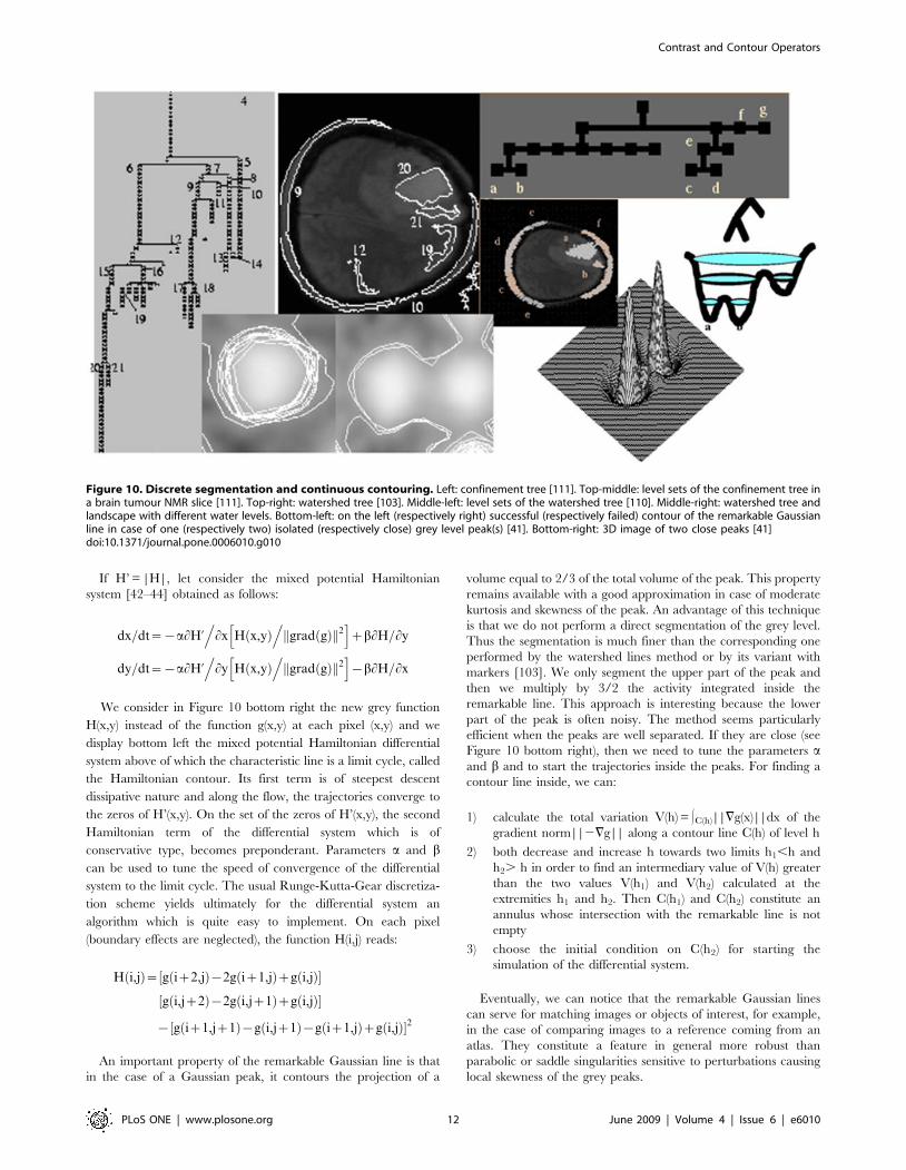
An important property of the remarkable Gaussian line is that

in the case of a Gaussian peak, it contours the projection of a

volume equal to 2/3 of the total volume of the peak. This property

remains available with a good approximation in case of moderate

kurtosis and skewness of the peak. An advantage of this technique

is that we do not perform a direct segmentation of the grey level.

Thus the segmentation is much finer than the corresponding one

performed by the watershed lines method or by its variant with

markers [103]. We only segment the upper part of the peak and

then we multiply by 3/2 the activity integrated inside the

remarkable line. This approach is interesting because the lower

part of the peak is often noisy. The method seems particularly

efficient when the peaks are well separated. If they are close (see

Figure 10 bottom right), then we need to tune the parameters aand b and to start the trajectories inside the peaks. For finding a

contour line inside, we can:

1) calculate the total variation V(h) = #C(h)||=g(x)||dx of the

gradient norm||2=g|| along a contour line C(h) of level h

2) both decrease and increase h towards two limits h1,h and

h2. h in order to find an intermediary value of V(h) greater

than the two values V(h1) and V(h2) calculated at the

extremities h1 and h2. Then C(h1) and C(h2) constitute an

annulus whose intersection with the remarkable line is not

empty

3) choose the initial condition on C(h2) for starting the

simulation of the differential system.

Eventually, we can notice that the remarkable Gaussian lines

can serve for matching images or objects of interest, for example,

in the case of comparing images to a reference coming from an

atlas. They constitute a feature in general more robust than

parabolic or saddle singularities sensitive to perturbations causing

local skewness of the grey peaks.

Figure 10. Discrete segmentation and continuous contouring. Left: confinement tree [111]. Top-middle: level sets of the confinement tree ina brain tumour NMR slice [111]. Top-right: watershed tree [103]. Middle-left: level sets of the watershed tree [110]. Middle-right: watershed tree andlandscape with different water levels. Bottom-left: on the left (respectively right) successful (respectively failed) contour of the remarkable Gaussianline in case of one (respectively two) isolated (respectively close) grey level peak(s) [41]. Bottom-right: 3D image of two close peaks [41]doi:10.1371/journal.pone.0006010.g010



Watershed contouring. The watershed line is a concept

firstly defined by geographers in order to characterize the main

features of a landscape: a drop of rain that reaches the ground will

flow down to a sea or an ocean. In the case of France, the

watershed line splits the country in two parts, the Atlantic zone

and the Mediterranean zone. Those zones are called ‘catchment

basins’, and the oceans are the minima of them, i.e. the attraction

basins of the gradient operator which corresponds to the

gravitational dynamics of the drop on the steepest gradient lines

of the relief surface. They define a partition of this relief, and the

boundaries of catchment basins define on the pixels plane the

watershed lines [105–109]. These lines are confounded in regular

cases with the crest lines surrounding the catchment basin. It is

easy to understand the interest of this concept in image processing:

grey level images can be considered as relief structures, and the

watershed lines are a good way to separate light (low grey level)

zones from dark (high grey level) ones. It is particularly interesting

to determine the watershed lines of the symmetrical reverse

landscape obtained by considering the new grey level 1-g, where g

is the initial normalized grey level obtained after the contrasting

step and after fixing the maximum of g as a normalized value

equal to 1. The watershed lines verify variational principles: i)

when progressively fulfilling with water a catchment basin, its

inner area passes through a series of inflexion points corresponding

to the successive saddle points reached by the water. Each

inflexion point corresponds to a local maximum of the second

derivative of the inner area; ii) for a given inner area, the

watershed lines are those containing the maximum of water. The

watershed line is computed on a discrete image, by immersion

simulation, locating it on the meeting points of several catchment

basins (Figure 10). First discrete algorithms of watershed lines

computed by immersion simulation were proposed in [105–109]

with a discrete operator. In [103,110], the watershed line is

computed on the reverse image, in order to have one and only one

local maximum of the original image into each catchment basin of

the reverse image. The resulting labelling (still not a partition) is

done on the original image. We used the Vincent-Soille algorithm

[105] on discrete images with a linear complexity (about 7,25 n,

where n denotes the number of pixels in the image). It can be used

also in 3 dimensions.

Reaction-diffusion contrasting. Several methods of image

contrasting by using differential linear or non-linear operators

have been proposed [92–99]. These methods can be parallelized

as for the neural networks and we will show in the following that

there exists a deep relationship between the discrete neural

network approach and the continuous differential operator

approach.

1) The Catte-Lions-Morel-Coll non-linear diffusionoperator. It is well known that the solution of the heat

differential operator:

Lu=Lt~k:Du~k:div grad uð Þð Þ

is the Gaussian kernel, with variance equal to s2 = 2 kt, by

choosing as initial conditions u(.,0) the grey level. This

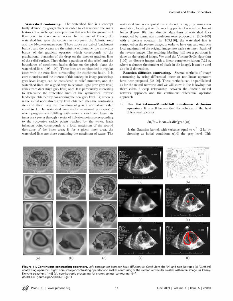
Figure 11. Continuous contrasting operators. Left: comparison between heat diffusion (a), Catte-Lions (b) [94] and non-isotropic (c) [93,95,96]contrasting operators. Right: non-isotropic contrasting operator and snakes contouring of the cardiac ventricular cavities with initial image (a), Canny-Deriche treatment [146] (b), non-isotropic processing (c), snakes splines contouring (d–f)doi:10.1371/journal.pone.0006010.g011



property has suggested [94] the use of another differential

non-linear diffusion operator:

Lu=Lt~div g grad G � uð Þkkð Þ:grad uð Þð Þ,

where G is a Gaussian kernel and g is a non-negative non-

increasing function on R+ verifying g(0) = 1 and g tends to 0

at infinity; in practice, we can choose for g a set function,

whose value is 1 on the interval [0,S] and 0 on]S, +‘[: there

is diffusion if and only if ||grad(G*u)||#S and, after a

certain transient, it remains a gradient only on the boundary

of sufficiently discriminable objects. For example, Figure 11

presents images after some hundreds of iterations, showing

the gradient on the boundary of brain structures. The end of

the procedure as for the heat operator (Figure 11 left (a))

shows that diffusion wins, giving a constant grey level at the

asymptotic state. In order to improve the method of getting

the contrasted image at the asymptotic state of the simulation,

we must add a reaction term in order to obtain the final

expected image as the attractor of a differential reaction-

diffusion operator, like for the iterative discrete neural

network as in Figure 11 left (c).

2) The non-isotropic reaction-diffusion operator. By

searching a continuous operator having as discrete finite

elements scheme a deterministic neural network system

similar to that presented in Section 2, it has been proposed

[93,95,96] with direct reference to the discrete neural

network approach [48,49,52] a new reaction-diffusion

operator. Let us recall the deterministic neural network with

threshold 0 defined by:

xi tz1ð Þ~1,

if Hi tð Þ~X

wijxj tð Þ w 0,

j[V ið Þ

~0, if Hi tð Þ~X

wijxj tð Þ ƒ 0,

j[V ið Þ

where V(i) is a neighbourhood of i. If we suppose the neural

network to be 2D and infinite, lets us denote by (i1, i2) the

position of the neuron i, where i M Z2; if wij are symmetrical

and translation invariant with finite range R, where R is the

radius of the neighbourhood V(0) of 0, there exists T defined

on [21,1]2 and valued in [21,1] such as:

wij~T i1{j1ð Þh=R, i2{j2ð Þh=Rð Þ,

where h is a strictly positive real number, T has as mean value

m,

m~

ðT y1,y2ð Þdy1dy2w0

and variance

s2~M{m2,

wherein

M~

ðT2 y1,y2ð Þdy1dy2:

Let us denote now by f a continuous regularized version of

the Heaviside function (like the arc-tan) and let us take

F~f{1,

a uð Þ~lR4S�

h2F’ uð Þ� �

,

b uð Þ~ {F uð ÞzlR2�

h2mu� ��

F’ uð Þ

then the reaction-diffusion operator defined by:

Lu=Lt~a uð ÞDuzb uð Þ

has a natural discretization corresponding to the neural

network above, by identifying xi(t) and u(ih,t) and by

remarking that the neural network system has the same

asymptotic behaviour as the differential system:

dxi tð Þ=dt~ lX

wij xj tð Þ{H xi tð Þð Þ� �.

H0 H xi tð Þð Þð Þ,

when l is sufficiently large. In [93], it is shown that, for

adapted values of R, homogeneous in grey, 1D objects can be

enhanced in a heterogeneous environment, in the same way

as for a neural network system. In [96] and in Figure 11

(right), the same proof is given for 2D objects like the internal

cavities of the heart, where a snakes splines procedure is used

after contrasting.

3) Proposal for a new image reaction-diffusion-chemo-taxis operator. In order to have, like for the previous

operator, the final treated image as asymptotic of a

differential operator, we propose to consider the grey level

u as a chemotactic substrate concentration consumed by

animals whose concentration will be denoted by v

[84,85,144]. The principle of this method consists in locating

initially a uniform concentration v(0) of animals on the initial

grey level image u(0) or on its boundary: the substrate u can

diffuse with a term eDu and is consumed with a saturation

rate equal to: 2Kuv/(u+k); the animal concentration v can

diffuse attracted by the substrate with the term DDv, is

submitted to a drift in the direction of substrate peaks with the

chemotactic term - xdiv(vgradu) and increases (because of the

reproduction) with the term K’uv(u+k’). Let us remark that

the two first terms ruling the animal motion can be replaced,

if we do not want to introduce a drift term, by an attraction-

diffusion term like:

D L2v�Lx2:Lu=LxzL2v

�Ly2:Lu=Ly

� �The corresponding differential partial derivative operator is

then given by:

Lu=Lt~eDu{Kuv= uzkð Þ,

Lv=Lt~DDv{xdiv vgraduð ÞzK0uv uzk0ð Þ

or by the following PDE:

Lu=Lt~eDu{Kuv= uzkð Þ

Lv�Lt~D L2v

�Lx2:Lu=LxzL2v

�Ly2:Lu=Ly

� �zK0uv= uzk0ð Þ



In the two cases above, the asymptote of u is 0 and the

asymptotes of v give the ‘‘treated image’’. The corresponding

image processing leads to a contrast enhancement before

segmentation: in Figure 7, we can see the initial image on the

bottom left and the contrasted one on the bottom right. The

contours have been then easily obtained by applying a snakes

splines procedure [71,72]. If we are adding to the second

equation of the differential system a Dupin term like Kv/Du,

we will encourage animals to follow Dupin lines, i.e. inflexion

curves, which is very suitable for a grey anticlines segmen-

tation (for example in vessels segmentation).

ConclusionThe neuro-mimetic lateral inhibition mechanism and the set

valued snakes-like flows allow the generation of various image

processing methods (essentially contrast enhancement and con-

touring). We have given numerous applications of this method-

ological approach in image processing essentially dedicated to

medical imaging and surgical robotics. Further both theoretical

and numerical studies have to be completed, in order to show the

utility of these new tools in morphogenesis modelling, allowing to

generate artificial objects of biological and/or medical interest (like

cells, tissues, organs) by using the same operators as for

recognizing them in a real image. We conjecture that the spatial

information about anatomic organs obtained from the biomimetic

image-processing methods, has to do with the morphogens

localization, which results from the morphogenetic processes

creating these organs combining robust genetic regulatory

networks [145,146] ruling their metabolic reactions and cell

proliferation, with classical diffusion [147] of morphogens inside

their tissues. In particular, the main patterns observed during the

embryonic formation can be found in the biomimetic processing of

the images by the final adult organ.

Acknowledgments

We are indebted to J. Mattes for helpful discussions and comments and to

E. Greene for many suggestions and improvements.

Author Contributions

Analyzed the data: YF MT NV. Wrote the paper: JD.

References

1. Hammond P (1971) Chromatic sensitivity and spatial organization of cat visual

cortical cells: cone-rod interaction. J Physiol 213: 475–494.

2. Attwell D, Werblin FS, Wilson M, Wu SM (1983) A sign-reversing pathwayfrom rods to double and single cones in the retina of the Tiger Salamander.

J Physiol 336: 313–333.

3. Signal Processing. Initial Processing of Visual Input in the Retina http://

education.vetmed.vt.edu/curriculum/VM8054/EYE/CNSPROC.HTM.

4. Eysel UT, Worgotter F, Pape HC (1987) Local cortical lesions abolish lateral

inhibition at direction selective cells in cat visual cortex. Exp Brain Res 68:

606–612.

5. Chubb C, Sperling G, Solomon JA (1989) Texture interactions determine

perceived contrast. Proc Natl Acad Sci USA 86: 9631–9635.

6. Burr DC, Morrone M (1990) Feature Detection in biological and artificialvisual systems. In: Blakemore C, ed. Vision Coding and Efficiency. Cambridge:

Cambridge Unversity Press. pp 185–194.

7. Solomon JA, Sperling G, Chubb C (1993) The lateral inhibition of perceived

contrast is indifferent to on- center/off-center segregation, but specific toorientation. Vision Res 33: 2671–2683.

8. Li Z (2000) Pre-attentive segmentation in the primary visual cortex. Spatial

Vision 13: 25–50.

9. Meir E, von Dassow G, Munro E, Odell G (2002) Robustness, Flexibility, and

the Role of Lateral Inhibition in the Neurogenic Network. Current Biology 12:

778–786.

10. Petrov Y, Carandini M, McKee S (2005) Two Distinct Mechanisms of

Suppression in Human Vision. J Neuroscience 25: 8704–8707.

11. Goldberg SH, Frumkes TE, Nygaard RW (1983) Inhibitory influence ofunstimulated rods in the human retina: evidence provided by examining cone

flicker. Science 221: 180–182.

12. Lyubarsky AL, Lem J, Chen J, Falsini B, Iannaccone A, et al. (2002)

Functionally rodless mice: transgenic models for the investigation of conefunction in retinal disease and therapy. Vision Res 42: 401–415.

13. Bilotta J, Powers MK (1991) Spatial contrast sensitivity of goldfish: mean

luminance, temporal frequency and a new psychophysical technique. VisionRes 31: 577–585.

14. Williams GA, Daigle KA, Jacobs GH (2005) Rod and cone function in coneless

mice. Vis Neurosci 22: 807–816.

15. Umino Y, Solessio E, Barlow RB (2008) Speed, Spatial, and Temporal Tuning

of Rod and Cone Vision in Mouse. J Neuroscience 28: 189–198.

16. Kawamura S, Tachibanaki S (2008) Rod and cone photoreceptors: Molecularbasis of the difference in their physiology. Comparative Biochemistry and

Physiology Part A 150: 369–377.

17. Burr EG (1947) Illumination for Concealment of Ships at Night Transactions.

Royal Soc Canada 41: 45–54.

18. von Bekezy J (1967) Mach band type lateral inhibition in different sense organs.

General Physiology 50: 519–532.

19. Leveillard T, Mohand-Saıd S, Lorentz O, Hicks D, Fintz AC, et al. (2004)Identification and characterization of rod-derived cone viability factor. Nature

Genetics 36: 755–759.

20. Corbo JC, Cepko CL (2005) A hybrid photoreceptor expressing both rod and conegenes in a mouse model of enhanced s-cone syndrome. PLoS Genet 1(2): e11.

21. Girman SV, Wang S, Lund RD (2005) Time course of deterioration of rod and

cone function in RCS rat and the effects of subretinal cell grafting: a light- anddark-adaptation study. Vision Research 45: 343–354.

22. Blankenship T (1987) Real-time enhancement of medical ultrasound images.

In: Kessler LW, ed. Acoustical Imaging. New York: Plenum. pp 187–195.

23. Martin JP (1988) Fast enhancement technique for PC-based image processing

systems. Diagnostic Imaging Magazine 1: 194–198.

24. Waxman AM, Seibert M, Cunningham R, Jian W (1988) The neural analog

diffusion enhancement layer (NADEL) and early visual processing. SPIE 1001:

1093–1102.

25. Khellaf A, Beghdadi A, Dupoisot H (1991) Entropic contrast enhancement.

IEE Trans Med Im 10: 589–592.

26. Le Negrate A, Beghdadi A, Dupoisot H (1992) An image enhancement

technique and its evaluation through bimodality analysis. CGVIP Graphical

Models and Image Processing 54: 13–22.

27. Toet A (1992) Multiscale contrast enhancement with applications to image

fusion. Optical Engineering 31: 1026–1031.

28. Neycenssac F (1993) Contrast enhancement using the Laplacian of a Gaussian

filter. CVGIP: Graphical Models and Image Processing 55: 447–463.

29. Ning F, Ming C (1993) An automatic cross-over point selection technique for

image enhancement using fuzzy sets. Pattern Rec Letters 14: 397–406.

30. Jian L, Healy Jr DM, Weaver JB (1994) Contrast enhancement of medical

images using multiscale edge representation. Optical Engineering 33:

2151–2161.

31. Demongeot J, Mattes J (1995) Neural networks and contrast enhancement in

medical imaging. In: Fogelman-Soulie F, Gallinari P, eds. ICANN’95. Paris:

EC2. pp 41–48.

32. Mattes J, Trystram D, Demongeot J (1998) Parallel image processing:

application to gradient enhancement of medical images. Parallel Processing

Letters 8: 63–76.

33. Rizzi A, Gatta C, Marini D (2003) A new algorithm for unsupervised global

and local colour correction. Pattern Recognition Letters 24: 1663–1677.

34. Tayyab M (2008) Segmentation and Contrasting in Retinal Images. Master

Thesis. Grenoble: University J. Fourier.

35. Thom R (1972) Stabilite structurelle et morphogenese. Paris: Intereditions.

36. Cosnard M, Demongeot J (1985) Attracteurs: une approche deterministe. CR

Acad Sci 300: 551–556.

37. Demongeot J, Jacob C (1989) Confineurs: une approche stochastique. CR

Acad Sci 309: 699–702.

38. Outrata JV (1990) On generalized gradients in optimization problems with set-

valued constraints. Mathematics of Op Research 15: 626–639.

39. Radcliffe T, Rajapakshe R, Shalev S (1994) Pseudocorrelation: a fast, robust,

absolute, grey-level image alignment algorithm. Medical Physics 21: 761–769.

40. Tonnelier A, Meignen S, Bosch H, Demongeot J (1999) Synchronization and

desynchronization of neural oscillators: comparison of two models. Neural

Networks 12: 1213–1228.

41. Demongeot J, Francoise JP, Richard M, Senegas F, Baum TP (2002) A

differential geometry approach for biomedical image processing. Comptes

Rendus Acad Sci Biologies 325: 367–374.

42. Demongeot J, Glade N, Forest (2007) Lienard systems and potential-

Hamiltonian decomposition. I Methodology. Comptes Rendus Acad Sci

Mathematique 344: 121–126.

43. Demongeot J, Glade N, Forest L (2007) Lienard systems and potential-

Hamiltonian decomposition. II Algorithm. Comptes Rendus Acad Sci

Mathematique 344: 191–194.



44. Glade N, Forest L, Demongeot J (2007) Lienard systems and potential-

Hamiltonian decomposition. III Applications in biology. Comptes RendusAcad Sci Mathematique 344: 253–258.

45. Herve T, Demongeot J (1988) Random field and tonotopy: simulation of an

auditory neural network. Neural Networks 1: 297.

46. Berthommier F, Demongeot J, Schwartz JL (1989) A neural net for processingof stationary signals in the auditory system. In: IEE Conf Signal Proc London.

London: IEE, London. pp 287–291.

47. Herve T, Dolmazon JM, Demongeot J (1990) Random field and neural

information: a new representation for multi-neuronal activity. Proc Natl Acad

Sci 87: 806–810.

48. Berthommier F, Francois O, Marque I, Cinquin P, Demongeot J, et al. (1991)

Asymptotic behaviour of neural networks and image processing. In:

Babloyantz A, ed. Self-Organization, Emerging properties and Learning.

New York: NATO Series Plenum Press. pp 219–230.

49. Leitner F, Marque I, Berthommier F, Cinquin P, Demongeot J, et al. (1991)

Neural networks, differential systems and image processing. In: Simon JC, ed.

From Pixels to Features II. Amsterdam: North Holland. pp 253–274.

50. Toborg ST, Huang K (1991) Cooperative vision integration through data-

parallel neural computations. IEEE Trans on Computers 40: 1368–1380.

51. Francois O, Demongeot J, Herve T (1992) Convergence of self-organizing

stochastic neural network processes. Neural Networks 5: 277–282.

52. Berthommier F, Bouchard V, Brunie L, Cinquin P, Demongeot J, et al. (1993)Medical imaging and modelling using a MasPar. In: Joubert GR, ed.

Proceedings PARCO 93. Parallel computing: trends and applications.

Amsterdam: Elsevier. pp 477–480.

53. Vinod VV, Chaudhury S, Mukherjee J, Ghose S (1994) A connectionist

approach for clustering with applications in image analysis. IEEE Trans onSystems, Man and Cybernetics 24: 365–385.

54. Brunie L, Leitner F, Berthommier F, Cinquin P, Demongeot J (1995)

Interpretation of multimodal medical images using connectionist and

variational methods. Technology and Health Care 3: 91–100.

55. Mattes J, Trystram D, Demongeot J (1995) Neural networks for parallel

contrast enhancement in medical images. In: Hertzberger LO, Serazzi G, eds.

High performance computing and networking. Lecture Notes in Comp Sci

919: 275–280.

56. Bosch H, Milanese R, Labbi A, Demongeot J (1998) Rate and TemporalCoding with a Neural Oscillator. In: Int Conf on Artif Neural Networks

(ICANN’98). London: Springer Verlag. pp 1021–1026.

57. Demongeot J, Berger F, Baum TP, Thuderoz F, Cohen O (2002) Bio-array

images processing and genetic networks modelling. In: Unser M, Liang ZP, eds.

ISBI 2002, IEEE EMB. Piscataway: IEEE Proceedings. pp 50–54.

58. Demongeot J, Thuderoz F, Baum TP, Berger F, Cohen O (2003) Bio-array

images processing and genetic networks modelling. Comptes Rendus Biologies

326: 487–500.

59. Fay DA, Waxman AM (1991) Real-time early vision neurocomputing. In:

International Joint Conference on Neural Networks. Piscataway: IEEE

Proceedings. pp 621–626.

60. Kobayashi H, Matsumoto T, Yagi T, Shimmi T (1991) A layered architecture

for regularization vision chips. In: International Joint Conference on Neural

Networks. Piscataway: IEEE Proceedings. pp 1007–1020.

61. Nabet B, Darling RB, Pinter RB (1992) Implementation of front-end processor

neural networks. Neural Networks 5: 891–902.

62. Kobayashi H, Matsumoto T, Yagi T, Shimmi, T (1993) Image processingregularization filters on layered architecture. Neural Networks 6: 327–350.

63. Shi BE, Roska T, Chua LO (1993) Design of linear cellular neural networks for

motion sensitive filtering. IEEE Trans Circuits Systems 40: 320–332.

64. Kobayashi N, Saito H, Nakajima M (1994) Fast adaptive contrast enhancementmethod for the display of gray-tone images. Trans IEICE 77: 502–509.

65. Kobayashi Y, Kato T (1999) A High Fidelity Contrast Improving Model Based

on Human Vision Mechanisms. In: Multimedia Computing and Systems.

Piscataway: IEEE Proceedings. pp 578–584.

66. Moini A (2000) Vision chips. Boston: Kluwer.

67. Kwon TM, Zervakis ME (1992) Design of regularization filters with linear

neural networks (image restoration. In: Conf. on Systems, Man & Cybernetics.

Piscataway: IEEE Proceedings. pp 416–421.

68. Nakahira H, Maruyama M, Ueda H, Yamada H (1993) An image processing

system using image signal multiprocessors (ISMPs). Journal of VLSI Signal

Processing 5: 133–140.

69. Mumford D, Shah J (1985) Boundary detection by minimizing functional. In:CVPR’85. Piscataway: IEEE Proceedings. pp 22–26.

70. Kass M, Witkin MA, Terzopoulos D (1987) Snakes: active contour models.

Int J Comp Vision 1: 321–331.

71. Leitner F, Marque I, Lavallee S, Cinquin P (1990) Dynamic Segmentation:

Finding the Edge with Snake- Splines. In: Laurent PJ, ed. Curves and Surfaces.

London: Academic Press. pp 279–284.

72. Cohen LD (1991) On active contour models and balloons. Computer Vision

Image Understanding 53: 211–218.

73. Chou WS, Chen Y (1993) Estimation of the velocity field of 2-d deformable

motion. Pattern Recognition 26: 351–364.

74. Chen Y, Medioni G (1995) Description of complex objects from multiple range

images using inflating balloon model. Computer Vision Image Understanding61: 325–334.

75. Kichenassamy S, Kumar A, Olver P, Tannenbaum A, Yezzi JR (1995)Gradient flows and geometric active contour models. In: ICCV. Piscataway:

IEEE Proceedings. pp 810–815.

76. Bainville E (1995) 3D reconstruction using a new dynamic model: the d-snakes.

Grenoble: Research Report TIMC-IMAG University J. Fourier.

77. Faugeras O, Keriven R (1999) Complete Dense Stereovision Using Level Set

Methods. Lecture Notes in Computer Science 1406: 379–393.

78. Sethian JA (1999) Level Set Methods and Fast Marching Methods.Cambridge, UK: Cambridge University Press.

79. Osher S, Fedkiw RP (2006) Level Set Methods: An Overview and Some RecentResults. Journal of Computational Physics 169: 463–502.

80. Jiang T, Tomasi C (2006) Level-Set Curve Particles. Lecture Notes inComputer Science 3953: 633–644.

81. Doyen L (1995) Mutational equations for shapes and vision-based control.

J Math Imaging Vision 5: 99–109.

82. Demongeot J, Leitner F (1996) Compact set valued flows I: applications in

medical imaging. CR Acad Sci 323: 747–754.

83. Lorenz T (2001) Compact set valued operator. Comp Vis Sci 4: 41–57.

84. Demongeot J, Bezy-Wendling J, Mattes J, Haigron P, Glade N, et al. (2003)

Multiscale Modeling and Imaging: The Challenges of Biocomplexity. Proc

IEEE 91: 1723–1737.

85. Demongeot J (2004) Dynamical Systems and Bio-medical Image Processing.WSEAS Trans Biol Inf Sc Appl 1: 618–623.

86. Demongeot J (2007) A brief history about the analytic tools in medical imaging:splines, wavelets, singularities and partial differential equations. In: IEEE

EMBC 07. Piscataway: IEEE Proceedings. pp 3474–3480.

87. Forest L, Michon F, Cadau S, Demongeot J, Dhouailly D (2006) What is the

biological basis of pattern formation of skin lesions? Viewpoint 4. Skin Patternsbelong to three main types, determined at three steps of development. Exp

Dermatol 12: 559–564.

88. Forest L, Demongeot J (2006) Cellular modelling of secondary radial growth in

conifer trees: application to Pinus radiata. Bull Math Biol 68: 753–784. DOI10.1007/s11538-005-9004-5.

89. Forest L, Martinez S, Padilla F, Demongeot J, San Martin J (2006) Modellingof auxin transport affected by gravity and differential radial growth. J Theor

Biol 241: 241–251.

90. Forest L, Demongeot J (2008) A general formalism for tissue morphogenesis

based on cellular dynamics and control system interactions. Acta Biotheoretica56: 51–74.

91. Michon F, Forest L, Collomb E, Demongeot J, Dhouailly D (2008) BMP-2 andBMP-7 play antagonistic roles in feather induction. Development 135:

2797–2805.

92. Perona P, Malik J (1990) Scale-space and edge detection using anisotropic

diffusion. IEEE Transactions on Pattern Analysis and Machine Intelligence 12:629–639.

93. Cottet GH (1991) Modeles de reaction-diffusion pour des reseaux de neuronesstochastiques et deterministes. CR Acad Sci 312: 217–221.

94. Catte F, Lions PL, Morel JM, Coll T (1992) Image selective smoothing and

edge detection by nonlinear diffusion. SIAM J Numer Anal 29: 182–193.

95. Cottet GH, Germain L (1993) Image processing through reaction combined

with nonlinear diffusion. Math Comp 61: 659–673.

96. Cottet GH, Demongeot J, El Ayyadi M, Leitner F (1995) Image segmentation

using snake-splines and anisotropic diffusion operators. Avalaible: http://tel.archives-ouvertes.fr/tel-00004940/en/.

97. Weickert J (1999) Coherence-Enhancing Diffusion Filtering. InternationalJournal of Computer Vision 31: 111–127.

98. Tschumperle D, Deriche R (2000) Restauration d’images vectorielles par EDP.

In: 12eme Congres RFIA‘00, Vol. II. Paris: AFCET. pp 247–256.

99. Tschumperle D, Deriche R (2002) Diffusion PDE’s on Vector-Valued Images.

Signal Processing Magazine 19: 16–25.

100. Meunier J, Bertrand M, Mailloux GE, Petitclerc R (1988) Assessing local

myocardial deformation from speckle tracking in echography. SPIE 914:20–29.

101. Mailloux GE, Langlois F, Simard PY, Bertrand M (1989) Restoration of thevelocity field of the heart from 2D echocardiograms. IEEE Trans Med Imaging

8: 143–153.

102. Leitner F, Paillasson P, Ronot X, Demongeot J (1995) Dynamical functional

and structural analysis of living cells: new tools for vital staining of nuclearDNA and for characterization of cell migration. Acta Biotheoretica 43:

299–317.

103. Demongeot J, Richard M (2000) New segmenting and matching algorithms as

tools for modelling and comparing medical images. In: Deville M, Owens R,eds. XVIth Imacs World Congress 2000. Lausanne: EPFL. pp 127–131.

104. Montanvert A, Meer P, Rosenfeld A (1991) Hierarchical image analysis usingirregular tesselations. IEEE Trans Pattern Anal Machine Intell 13: 307–316.

105. Vincent L, Soille P (1991) Watershed in Digital Spaces: an Efficient Algorithm

Based on Immersion Simulations. IEEE Transactions on Pattern analysis and

Machine Intelligence 13: 583–598.

106. Meyer F (1992) Un algorithme optimal de ligne de partage des eaux. In:

VIIIeme Conf Reconnaissance des Formes et Intelligence Artificielle. Paris:AFCET. pp 847–859.

107. Beucher S, Meyer F (1993) The morphological approach to segmentation: the

watershed transformation. In: Dougherty ER, ed. Mathematical Morphology

in Image Processing. New York: Marcel Dekker. pp 433–481.



108. Bertrand G, Everat JC, Couprie M (1997) Topological gray scale watershed

transformation SPIE 3168: 136–146.109. Bertrand G, Everat JC, Couprie M (1997) Image segmentation through

operators based upon topology. Journal of Electronic Imaging 6: 395–405.

110. Mattes J, Richard M, Demongeot J (1999) Tree representation for imagematching and object recognition. Lecture Notes in Comp Sci 1568: 298–309.

111. Mattes J, Demongeot J (1999) Tree representation and implicit tree matchingfor a coarse to fine image matching algorithm. Lecture Notes in Comp Sci

1679: 646–655.

112. Mattes J, Demongeot J (1999) Dynamic confinement, classification andimaging. Springer Studies in Classification Data Anal Knowledge Org 14:

205–214.113. Mattes J, Demongeot J (2000) Comparison of error measures in confinement

tree based matching. In: ICARCV 2000. Singapore: NTU Ed. pp 3–8.114. Richard M, Fleute M, Desbat L, Lavallee S, Demongeot J (2000) Registration

of medical images. SPIE 3831: 125–139.

115. Mattes J, Demongeot J (2001) Efficient algorithms to implement theconfinement tree. Lecture Notes in Comp Sci 1953: 392–405.

116. Mattes J, Demongeot (2001) Structural outlier detection for automaticlandmark extraction. SPIE 4322: 602–610.

117. Bertrand G (2007) On the dynamics. Image and Vision Computing 25:

447–454.118. Ouchchane L, Villeger A, Lemaire JJ, Demongeot J, Boire JY (2007) Analysis

and visualization of images overlapping: automated vs expert anatomicalmapping in deep brain stimulation targeting. Lecture Notes in Comp Sci 4370:

136–146.119. Benabid AL, Cinquin P, Lavallee S, Le Bas JF, Demongeot J, et al. (1987) A

computer driven robot for stereotactic surgery connected to cat-scan magnetic

resonance imaging. Technological design and preliminary results. AppliedNeurophysiology 50: 153–154.

120. Lavallee S, Cinquin P, Demongeot J, Benabid AL, Marque I, et al. (1989)Computer assisted interventionist imaging: the instance of stereotactic brain

surgery. In: Medinfo 89 Singapore. Amsterdam: North Holland. pp 613–617.

121. Lavallee S, Cinquin P, Demongeot J, Benabid AL, Marque I, et al. (1989)Computer assisted driving of a needle into the brain. In: Lemke HU,

Rhodes ML, Jaffe CC, Felix R, eds. Computer assisted radiology, ProceedingsCAR 89. Berlin: Springer Verlag. pp 416–420.

122. Cinquin P, Lavallee P, Demongeot J (1989) A new system for computer assistedneurosurgery. In: IARP’89 Medical and Healthcare Robotics Newcastle.

London: DTI. pp 63–66.

123. Benabid AL, Hoffmann D, Lavallee S, Cinquin P, Demongeot J, Le Bas JF,Danel F (1991) Is there any future for robots in neurosurgery ? In: Symon L, ed.

Advances and technical standards in neurosurgery. New York: SpringerVerlag. pp 4–45.

124. Cinquin P, Demongeot J, Troccaz J, Lavallee S, Champleboux G, Brunie L,

Leitner F, Sautot P, Mazier B, Perez A, Djaid M, Fortin T, Chenin M,Chapel A (1992) Igor: image guided operating robot. Methodology, medical

applications, results. ITBM 13: 373–393.125. Benabid AL, Lavallee S, Hoffmann D, Cinquin P, Demongeot J, et al. (1992)

Potential use of robots in endoscopic neurosurgery. Acta Neurochir 54: 93–97.126. Benabid AL, Lavallee S, Hoffmann D, Cinquin P, Demongeot J, et al. (1992)

Computer drived robot for stereotactic neurosurgery. In: Kelly PJ, ed.

Computers in stereotactic surgery. Cambridge: Blackwell Sc Pub. pp 330–342.127. Benabid AL, Lavallee S, Hoffmann D, Cinquin P, Demongeot J, et al. (1992)

Computer support for the Talairach system. In: Kelly PJ, ed. Computers instereotactic surgery. Cambridge: Blackwell Sc Pub. pp 230–245.

128. Benabid AL, Lavallee S, Hoffmann D, Cinquin P, Demongeot J, et al. (1992)

Stereotactic robot for neurosurgery. In: IEEE Neurosciences and Technology

Lyon.. Piscataway: IEEE Proceedings. pp 157–160.

129. Demongeot J (1995) Chirurgie assistee par ordinateur: bilan et perspectives.

Chirurgie 120: 300–307.

130. Fortin T, Coudert JL, Jourlin M, Demongeot J (1997) Computer Assisted

Dental Intervention. DentoMaxilloFacial Radiology 26: 284–285.

131. Bzostek A, Ionescu G, Carrat L, Barbe C, Chavanon O, et al. (1998) Isolating

moving anatomy in ultrasound without anatomical knowledge: Application to

computer-assisted pericardial punctures. Lecture Notes in Comp Sci 1496:

1041–1048.

132. Ionescu G, Lavallee S, Demongeot J (1999) Automated registration of

ultrasound with CT images: application to computer assisted prostate

radiotherapy and orthopedics. Lecture Notes in Comp Sci 1679: 768–777.

133. Vazquez-Buenos Aires JO, Payan Y, Demongeot J (2003) Electro-stimulation

of the tongue as a passive surgical guiding system. In: de Almeida AT, Nunes U,

eds. ICAR 03 Coimbra. Piscataway: IEEE Proceedings. pp 638–643.

134. Demongeot J (2005) Medical imaging and computer assisted therapy: some

new approaches. In: Troccaz J, ed. Surgetica 04. Paris: Sauramps Medical. pp

301–303.

135. Robineau F, Boy F, Orliaguet JP, Demongeot J, Payan Y (2007) Guiding the

surgical gesture using an electro-tactile stimulus array on the tongue: a

feasibility study. IEEE Trans BME 54: 711–717.

136. Fabre-Thorpe M, Delorme A, Marlot C, Thorpe S (2001) A limit to the speed

of processing in ultra-rapid visual categorization of novel natural scenes. J Cogn

Neurosci 13: 171–180.

137. Emmeche C, Hoffmeyer J (1991) From language to nature - the semiotic

metaphor in biology. Semiotica 84: 1–42.

138. Kergosien YL (1985) Semiotique de la nature. In: IVe Seminaire de l’Ecole de

Biologie Theorique, Solignac 4-7 juin 1984. Paris: Editions du CNRS. pp

11–26.

139. Pattee HH (1977) Dynamic and linguistic modes of complex systems.

Int J General Systems 3: 259–266.

140. Koendering JJ, van Doom AJ (1979) The internal representation of solid shape

with respect to vision. Biological Cybernetics 32: 211–216.

141. Dickinson SJ, Christensen HI, Tsotsos JK, Olofsson G (1997) Active object

recognition integrating attention and viewpoint control. Computer Vision and

Image Understanding 67: 239–260.

142. Arkachar P, Wagh MD (2007) Criticality of lateral inhibition for edge

enhancement in neural systems. Neurocomputing 70: 991–999.

143. Deriche R (1990) Fast algorithms for low-level vision. IEEE Trans Pattern

Analysis and Mach Intelligence 12: 78–87.

144. Meignen S (1998) Application au contrastage d’images d’un operateur

differentiel de type chimio-tactique. DEA IMAG, University J. Fourier

Grenoble.

145. Elena A, Ben-Amor H, Glade N, Demongeot J (2008) Motifs in regulatory

networks and their structural robustness. In: IEEE BIBE’ 08. Piscataway: IEEE

Proceedings, Piscataway. pp 234–242.

146. Ben Amor H, Demongeot J, Elena A, Sene S (2008) Structural Sensitivity of

Neural and Genetic Networks. In: MICAI’ 08, LNCS 5317: 973–986.

147. Fourier J (1808) Memoire sur la propagation de la Chaleur dans les corps

solides. Nouveau Bulletin des Sciences de la Societe Philomathique de Paris 6:

112–116.



Understanding Physiological and Degenerative Natural Vision Mechanisms to Define Contrast and Contour Operators

Documents