Understanding Network Performance Bottlenecks - UiO - DUO

Understanding NetworkPerformance Bottlenecks

Pratik TimalsenaMaster’s Thesis Autumn 2016

Understanding Network PerformanceBottlenecks

Pratik Timalsena

November 15, 2016

ii

Abstract

Over the past decade, the rapid growth of the Internet has challenged itsperformance. In spite of the significant improvement in speed, capacity,and technology, the performance of the Internet in many cases remainssuboptimal. The fundamental problem is congested links that causebottleneck leading to poor network performance. Apart from that, It iswidely accepted that most congestion lies in the last mile. However,the performance of a network is also deteriorated in the core networksnowadays as the peering links have been affected severely due to theoverburden of packets resulting in packet loss and poor performance.In the thesis, we investigated the presence and location of congestedlinks in the core networks and the edge networks on the Internet. Wemeasured end to end latency between over 200 node pairs from all over theworld in PlanetLab and identified congested node pairs among them. Thecongested links between two end nodes were identified using tracerouteanalysis. By locating congested links in a network, we examined congestionin the edge networks and the core networks. We observed congestionboth in the edge networks and the core networks, however, we detectedaround 58% congestion in the core networks and around 42% in the edgenetworks.

iii

iv

Contents

I Introduction 1

1 Introduction 31.1 Motivation . . . . . . . . . . . . . . . . . . . . . . . . . . . . . 4

1.1.1 Continuous and rapid growth of the Internet . . . . . 41.1.2 Slow Internet speed . . . . . . . . . . . . . . . . . . . 51.1.3 High Internet delay . . . . . . . . . . . . . . . . . . . . 51.1.4 Problems in the core Network . . . . . . . . . . . . . . 5

1.2 Problem Statement . . . . . . . . . . . . . . . . . . . . . . . . 5

2 Background 72.1 Internet . . . . . . . . . . . . . . . . . . . . . . . . . . . . . . . 7

2.1.1 A Brief History of Internet . . . . . . . . . . . . . . . . 72.1.2 Growth in the Internet . . . . . . . . . . . . . . . . . . 82.1.3 Internet Architecture . . . . . . . . . . . . . . . . . . . 102.1.4 Routing Protocol in the Internet . . . . . . . . . . . . 12

2.2 Congestion in the Internet . . . . . . . . . . . . . . . . . . . . 132.2.1 Distribution of congestion in the internet . . . . . . . 142.2.2 Congestion in the core of Internet . . . . . . . . . . . 142.2.3 Internet Buffer and Congestion . . . . . . . . . . . . . 142.2.4 Active Queue Management (AQM) . . . . . . . . . . 15

2.3 End to end delay measurement . . . . . . . . . . . . . . . . . 162.4 Performance Bottlenecks . . . . . . . . . . . . . . . . . . . . . 17

2.4.1 Types of Bottlenecks . . . . . . . . . . . . . . . . . . . 172.4.2 Bottlenecks behaviours . . . . . . . . . . . . . . . . . 18

2.5 Network Performance Metrics . . . . . . . . . . . . . . . . . . 192.6 PlanetLab Testbed . . . . . . . . . . . . . . . . . . . . . . . . . 20

II The project 272.7 Overview of the project . . . . . . . . . . . . . . . . . . . . . . 29

3 Experiments design and setup 313.1 Description and Procedure of Experiment . . . . . . . . . . . 32

3.1.1 Overview of the PlanetLab nodes involved in theExperiment . . . . . . . . . . . . . . . . . . . . . . . . 32

3.1.2 Hardware and System Information . . . . . . . . . . . 333.1.3 Experiments details . . . . . . . . . . . . . . . . . . . 33

v

III Analysis and Results 43

4 Latency Analysis 454.1 Classification of Datasets . . . . . . . . . . . . . . . . . . . . 454.2 Creating Time series data . . . . . . . . . . . . . . . . . . . . 464.3 Latency Trend over time . . . . . . . . . . . . . . . . . . . . . 46

4.3.1 Latency analysis on links from Asia to other continents 464.3.2 Latency Analysis on Links from America to Europe

and vice versa . . . . . . . . . . . . . . . . . . . . . . . 504.3.3 Latency analysis of links from Europe to Asia . . . . 574.3.4 Latency analysis of links from America to Asia . . . . 624.3.5 Latency analysis of links from America to America

and Europe to Europe . . . . . . . . . . . . . . . . . . 644.4 Idetification of congested links . . . . . . . . . . . . . . . . . 65

5 Traceroute Analysis 675.1 Parsing and retrieving data in designated format . . . . . . . 675.2 Generating Time series data for each hop from source to

destination . . . . . . . . . . . . . . . . . . . . . . . . . . . . 675.3 Analysis by correlation . . . . . . . . . . . . . . . . . . . . . 685.4 Results . . . . . . . . . . . . . . . . . . . . . . . . . . . . . . . 68

6 Discussion and Conclusion 736.1 Discussion on results from latency analysis . . . . . . . . . . 736.2 Discussion on traceroute analysis results . . . . . . . . . . . . 786.3 Limitations . . . . . . . . . . . . . . . . . . . . . . . . . . . . 796.4 Conclusion . . . . . . . . . . . . . . . . . . . . . . . . . . . . . 796.5 Future works . . . . . . . . . . . . . . . . . . . . . . . . . . . . 80

Appendices 85

vi

List of Figures

2.1 Growth trends of lnternet traffic, voice traffic, maximumtrunk speed, and maximum switch speed required for largecities. [37] . . . . . . . . . . . . . . . . . . . . . . . . . . . . . . 9

2.2 Internet users growth trend. [42] . . . . . . . . . . . . . . . . 92.3 Types of ISP [44] . . . . . . . . . . . . . . . . . . . . . . . . . . 112.4 External and Internal BGP [13] . . . . . . . . . . . . . . . . . 122.5 Packet drop functions with AQM and tail-drop. [38] . . . . . 162.6 PlanetLab European sites. [29] . . . . . . . . . . . . . . . . . . 202.7 The process of acquiring the slice [12] . . . . . . . . . . . . . 21

3.1 Overview of the component of experiment. . . . . . . . . . . 323.2 The Flow chart for Experiment. . . . . . . . . . . . . . . . . . 333.3 Tree view of File arrangement . . . . . . . . . . . . . . . . . . 40

4.1 The continent to continent sets and node pairs involved . . . 464.2 Latency trend over hours on the links from Asia to Europe Set 484.3 Latency trend over hours on the links from Asia to Europe Set 494.4 Latency trend over hours on the links from Asia to Europe Set 504.5 Classification of links in America to Europe by local time zone 514.6 Classification of links in Europe to america by local time zone 514.7 RTT Trend of links between Eastern US to Central Europe . . 524.8 RTT Trend of links between Western US to Central Europe . 534.9 RTT Trend of links between Pacific Day Time zone in US to

Central Europe . . . . . . . . . . . . . . . . . . . . . . . . . . 544.10 RTT Trend of links between Central Day Time zone in US to

Central Europe . . . . . . . . . . . . . . . . . . . . . . . . . . 554.11 RTT Trend of links between Pacific Day Time zone in the US

to Eastern Europe . . . . . . . . . . . . . . . . . . . . . . . . . 564.12 RTT Trend of links between Central Europe and Central US 584.13 RTT Trend of links between Europe to Pacific Day Time USA 594.14 RTT Trend of links between Europe to Mountain Day Time

US . . . . . . . . . . . . . . . . . . . . . . . . . . . . . . . . . 604.15 RTT Trend of links between Europe and Asia, Australia

Oceania . . . . . . . . . . . . . . . . . . . . . . . . . . . . . . . 614.16 RTT Trend of links between Europe and China . . . . . . . . 624.17 RTT Trend of links between Central Day Time zone in US to

China . . . . . . . . . . . . . . . . . . . . . . . . . . . . . . . . 63

vii

4.18 RTT Trend of links between Eastern Day Time zone in US toChina . . . . . . . . . . . . . . . . . . . . . . . . . . . . . . . . 64

4.19 List of links having congestion . . . . . . . . . . . . . . . . . 65

5.1 Number of the links with network position . . . . . . . . . . 695.2 Number of the links with Link type . . . . . . . . . . . . . . . 705.3 Number of the links with network position and link type . . 715.4 Number of the links with network position and link type . . 72

6.1 GMT to Local time chart . . . . . . . . . . . . . . . . . . . . . 736.2 Patterns of congested links after gathering the links with

similar RTT trend together . . . . . . . . . . . . . . . . . . . 746.3 Number of congested links along with Network position for

RTT patterns shown in figure 6.2 . . . . . . . . . . . . . . . . 766.4 RTT trend America to America . . . . . . . . . . . . . . . . . 776.5 RTT trend Europe to Europe . . . . . . . . . . . . . . . . . . . 786.6 Number of the links with network position and link type for

GEANT, ABILENE and CHINANET-BACKBONE backbonenetworks . . . . . . . . . . . . . . . . . . . . . . . . . . . . . . 79

viii

List of Tables

3.1 List of PlanetLab nodes with location information . . . . . . 34

ix

x

List of Algorithms

1 Select_best_nodes . . . . . . . . . . . . . . . . . . . . . . . . . 352 Select_Inter-domain_links_per_node . . . . . . . . . . . . . . 363 Collect_data_Every day . . . . . . . . . . . . . . . . . . . . . . 39

xi

xii

Preface

This thesis is submitted in a partial fulfillment of the requirements for aMaster’s Degree in Programming and Networks at the University of Oslo.My supervisors on this project have been Ahmed Elmokashfi, AndreasPetlund, and Pål Halvorsen. This thesis has been made solely by the au-thor; a lot of the contents, however, is based on the research of others, thereferences to these sources have been provided as far as possible. I wouldlike to thank Ahmed Elmokashfi and Andreas Petlund for their most valu-able supervision and worthy guidelines during whole master thesis. I amthankful to Pål Halvorsen for the participation in the thesis.

Finally, I would like to thank everyone who has been helpful and support-ive during my master thesis.

xiii

xiv

Part I

Introduction

1

Chapter 1

Introduction

Network performance has been a central research topic during the lastdecade. In reality, a network is designed in conjunction with its perfor-mance in mind. The performance is the service delivered by networks to itsusers. For example, the core business of a content delivery network hingeson its ability to deliver content at a predictable, consistent, and acceptableperformance.For the sake to achieve the high performance, a significant ef-fort has been made by improving speed, capacity, and technology. Despitespending a lot of money on upgrading technologies and resources, the net-work performance remains suboptimal[41]. The underlying problem is thecongested links which cause bottlenecks and plague the network perfor-mance. In addition, a data packet can travel with a speed of the light in atheory [40]. Then a serious question arises why it takes so long time to crossshort distances if the network is not congested. In this project, we investi-gate the prevalence of congestion in the wide area .

Although the Internet appears to be a single entity, it is a collection of thou-sands of different networks each providing connectivity to certain groupsof end users . From the economic point of view, a network can be viewed asa first mile (ie, web hosting), a middle mile and the last mile (ie,end users).A middle mile is the part of the network between the network core and lastmile providers, which comprises heterogeneous networks owned by mul-tiple highly competing entities often peering with each other or providingtransit service [35] .

It is generally accepted that most congestion lies in the last mile. This con-vention urged us to improve and speed up the last miles capacity. Underthis circumstance, the last miles capacity has increased 50 folds over thelast decade. The first miles in the network has also acquired attention andincreased the speed by 20 folds over last 5 to 10 years. However, the middlepart of a network or the core network has not enjoyed a similar growth. Thepeering links has been affected severely due to the overburden of packetsresulting in packet loss and poor performance. Hence, the myth of last milecongestion has been outdated as the network performance has deterioratedin the middle part of the network as well [30] . In this thesis, we have made

3

a small attempt to find the congested links in transit networks and the lastmile networks that are affecting the performance of the network.

In this project, We performed active end to end measurement with morethan 200 pairs that are part of the PlanetLab testbed. The nodes comprisingthe links are distributed all over the world. We selected node pairs suchthat they are located in different cities and belong to different networks, inorder to maximize the inter-peer network distance. We probed each link forthree weeks by sending packets from one end to another end and calculatedRTT for all the links. We first identified the congested node pair links withthe help of latency trend analysis. After that, we dug more into these con-gested links using traceroute. We performed correlation analysis betweenRTT and Hop by Hop delay for each hop on the path between the con-gested node pairs and found the congested links on the path. We locatedthe position of these links on the network and identified whether the linksare inter-domain links or intra-domain links. On basis of that information,we found that there are more congested links in transit networks than inlast mile networks. In addition, we detected more congested intra-domainlinks than congested inter-domain links.

1.1 Motivation

1.1.1 Continuous and rapid growth of the Internet

The evolution of the broadband Internet has facilitated video and audiostreaming on the Internet due to the availability of more bandwidth. At thesame time, the Internet is growing rapidly in terms of the number of usersand data traffic. Nowadays, there are more than 3 billion Internet users,generating a large amount of the data traffic. In the context of streamingdata on the internet , the video traffic has surpassed all other traffic such astext, image, and audio, within a short time frame. In addition, various mul-timedia and cloud applications have emerged to utilize the available band-width on the Internet. Content providers like Netflix and YouTube generateenormous traffic volumes which is causing troubles for access providers bycreating overloaded link due to congestion [42] .

The Introduction of the Smart Mobile phone and mobile broadband ser-vice has also contributed to the growth of the Internet traffic.Tthe mobiledata has surpassed the fixed broadband data nowadays and is still growingsignificantly[26] .

Hence, we can predict that increasing the capacity of the network will notbe sufficient for improving network performance. Since the network capac-ity will always be filled by data from new users and the applications, weneed to dig more into identifying the actual problems within a networksuch as congestion, bottleneck, delay, and loss. Thereafter, we can solve theproblems using some novel techniques.

4

1.1.2 Slow Internet speed

Because of congestion on the Internet, the end users are not receiving thequality of service they have expect. Users are complaining about the speedof the Internet and are not happy with a quality of the service. Nowadaysthey have reported that the broadband speed is not consistent and is slowand thus frustrates users as they did not get what they paid for. In the USonly 30% of online users received the advertised speed [10]. Furthermore,user expectation is very high especially when video streaming, VOIP,online gaming. Thus, when there is a delay and buffering while onlinestreaming or playing games, it might be frustrating for users. The mainpoint is that performance of the network is not satisfactory in terms of usersperspective because of congestion [] .

1.1.3 High Internet delay

The bufferbloats term has been coined to represent the large queuingdelays on the internet. The use of very large buffers often lead to highqueuing delay and thus contributes to network performance degradationand packet loss. As a result, the one-way trip delay can sometimes bearound one second and two-way delay can be few seconds. This much ofdelay is comparable to time for communication from earth to the moon andback to earth[11]. Hence, the delay is one of the performance degradingfactors, we need to investigate.

1.1.4 Problems in the core Network

The content provider routes their content via access providers to endconsumers. In this process, they send excessive traffic causing congestion inthe link between content providers and access provider or transit provider.The recent peering dispute between Netflix and Comcast reflects thescenario better which is explained in [16]. Netflix and Cogent suggestedthat Comcast made congestion on the route between Netflix and Cogentand forced for the direct interconnection.

1.2 Problem Statement

In the thesis, our goal is to examine congestion in the edge networks andcore networks. In order to address this problem, we will look through fol-lowing questions.1) Which links are congested ?2) Where in a network are congested links located ?3) Whether congested links are in Intra-domain networks or Inter-domainnetworks ?4) Where is more congestion (in the edge networks or in the core networks)?

5

6

Chapter 2

Background

2.1 Internet

A computer Network is a set of computing devices, which communicatevia a communication channel and share information, resources and data.The Internet is a giant network, which is a network of the networks thatconnects computers worldwide[33]. The internet might appear to be asingle big network but the Internet is not merely a single network. It isformed by collecting various small network with a complex architecturebeneath the surface of each. The group of networks under a singleadministration (Internet service provider or any large Institute) with adefined routing policy of its own is referred to as Autonomous system(AS).Moreover, Internet consists of about 50k Autonomous Systems controlledby ISPs (Internet Service providers), routers connecting them and protocolswhich facilitate the communication among them. We will discuss moreon this topic later [15]. In this section, we will discuss on the Internetarchitecture, history of the Internet, protocols and other topics central toInternet bottleneck measurements.

2.1.1 A Brief History of Internet

The history of the Internet began with the formation of the AdvancedResearch Projects Agency (ARPA) in 1958 in the US. The history of theInternet can be explained as evolution from ARPANET to NFSNET andto the commercial Internet that we have nowadays.After the establishment of ARPA, it was changed to DARPA (DefenseAdvanced Research Project Agency) and later changed back to ARPA.Thereafter, there was an ongoing research on packet switching both inacademia and industry with the US government being the intertwinedpartner. The feasibility of using packets instead of circuits was studiedand the concept of a computer network was realized. The first ARPANETplan was began as a design paper in 1967 meanwhile,the National PhysicalLaboratory (NPL) in England deployed an experimental network calledthe NPL using packet switching [28]. The world's first packet-switchingcomputer network was established in 1969 by connecting computers at

7

the University of California Los Angeles (UCLA), the Stanford ResearchInstitute (SRI), the University of Utah and University of California SantaBarbara (UCSB) using separate mini computer which worked as a gatewayfor packets and called as Interface Message Processors (IMPs). TheARPANET gradually expanded as thirty academic, military and otherresearch networks joined ARPANET by 1973. Due to the expansion of theARPANET, there was a demand for an agreed set of rules for handlingthe packets. Thus, computer scientists Bob Kahn and Vint Cerf proposed anew method of sending packets in the network in 1974 by using techniquepacket within the digital envelope. The packet can be transferred toany computer in the network but can only be opened from the digitalenvelope at the final destination. This technique was referred to as theTCP/IP protocol. After the introduction of the TCP/IP communicationamong networks were through a common ARPANET language and thenetwork grew significantly giving rise to a global interconnected networkof networks, or Internet [1].

2.1.2 Growth in the Internet

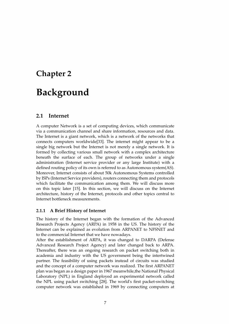
In 1969, the first Internet node was installed aiming to connect 15computers. After ongoing experiment for 4 years, 52 computers wereconnected. For 18 year the Internet hosts doubled every 15 monthsmeanwhile the network traffic were doubled every 12 months. The trendchanged drastically after 1997 after the introduction of Dense WavelengthDivision Multiplexing (DWDM), which lowered the communication costsby a half every 12 months, and hence doubling the network traffic everysix months. At the same time, the emergence of e-commerce also fuelledthe increasing trend of Internet traffic in a such a way that the pace ofthe growth was four times a year. Because of this reason, there was strongdemand for the improvement of the routers performance at a rate fasterthan 18 months doubling of semiconductor performance that Moore hadpredicted in 1975. The author [37] predicted that the same trend willcontinue until 2008 and after that as long as other methods to decrease costsof bandwidth is not introduced, the internet traffic growth will slow downas predicted in 1975. Figure 2.1 shows growth trends of Internet traffic,voice traffic, maximum trunk speed, and maximum switch speed requiredfor large cities.

8

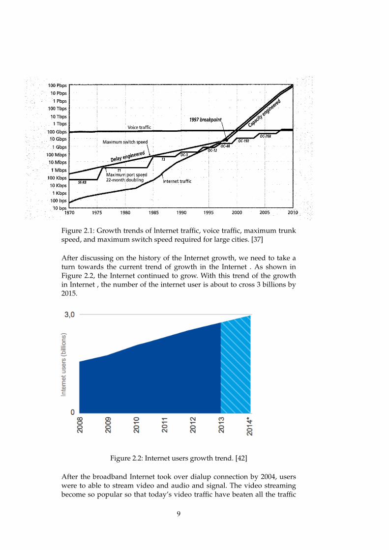
Figure 2.1: Growth trends of lnternet traffic, voice traffic, maximum trunkspeed, and maximum switch speed required for large cities. [37]

After discussing on the history of the Internet growth, we need to take aturn towards the current trend of growth in the Internet . As shown inFigure 2.2, the Internet continued to grow. With this trend of the growthin Internet , the number of the internet user is about to cross 3 billions by2015.

Figure 2.2: Internet users growth trend. [42]

After the broadband Internet took over dialup connection by 2004, userswere to able to stream video and audio and signal. The video streamingbecome so popular so that today’s video traffic have beaten all the traffic

9

such as audio, image, email in terms of volume. Another turning pointon the internet occurred with invention of the smartphone and Mobilebroadband Internet. The number of mobile users began to grow fasteras a result the mobile Internet user appeared in the significant figureamong the Internet users after 2008. Then the fixed broadband Internetaccess and Mobile Internet access grew continuously. However, mobileInternet access grew significantly than fixed broadband Internet. In thiscontext, the developing country exceeded the developed country on mobileInternet access. The global Internet access raised by 12% during 2008-2012.Thereafter 2012, the growth trend was slowed down from 10%annual growth to 5% for the broadband Internet access because themobile broadband Internet acess got an importance over it. [42]The authorpredicted that this trend will last until 2018 and mobile Internet user andMobile broadband Internet access is likely to flourish significantly as well.In this way, within this period,the mobile broadband Internet access willsurpass fixed broadband Internet access.[27]In the recent paper from Cisco, there is an update on the global mobiledata traffic forecast for the period between 2015 and 2020. According tothis report, the mobile data traffic grew 74 percent in 2015 as more thanhalf a billion (563 million) mobile devices and connections were added.Furthermore, the smart phone has contributed the most for the growth.They also predicted that mobile data traffic will increase nearly eightfoldbetween 2015 and 2020.From the above information, We can predict that due to the rapid growthof the internet the link will be overloaded. Hence, the available resourcemight not be enough to handle those internet traffic causing degradationon the performance due to congestion.

2.1.3 Internet Architecture

In this section, we will explain more about Autonomous System becausethe Autonomous System is a foundation of the Internet architecture.Thereafter, we will discuss on how do they interact in the network.

Autonomous System

Autonomous System is a collection of routers and protocols which operatethem and is owned by a single administrative domain. The routersexchange traffic within the AS using Interior gateway protocol such asRIP, OSPF and with other ASes using the border gateway protocol (BGP). Thus the ISPs communicate with each other via BGP while allowing theindividual ASes to implement their own policy. In addition, the interactionand relation among ISPs are governed by their policy and commercialagreement between the other ISPs as well[4].Commercial agreements can be classified into customer-provider andpeering. This also signifies what sort of relation and role do the ISPshave on the Internet. The ASes can play a role as service provider forcustomers. Customer pays the provider to get an internet connection.

10

Whereas in peering, the ASes agrees to exchange the traffic from theircustomer without any charge[18].

ISP Tier

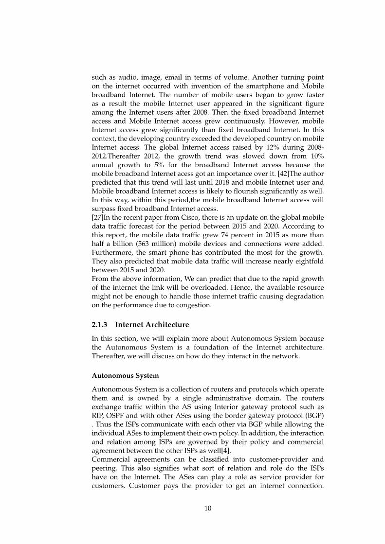
Mainly, ISP can be classified to Tier1, Tier2, and Tier3 ISP. On the basis ofthe size and the geographic coverage, Tier 1 is further divided on regionalTier1 and global. Figure 2.3 depicts the classification of the ISPs on the basisof the size and the geographical coverage.

Figure 2.3: Types of ISP [44]

A Tier 1 ISP has larger network and greater geographical coverage than aTier 2 ISP and a Tier 1 ISP. It has its own operating infrastructures includingrouters and other intermediate devices which constitute the backbone. TheTier 1 ISPs are connected to other Tier 1 ISPs or similar sized networks byprivate peering. They are interconnected at Internet Exchange points(IXPs).The global Tier 1 ISP have its own communication infrastructure or it canalso use the alternative carrier communicating circuit depending upon theagreement with other ISPs. Generally, the Tier 1 ISPs are ASes that covermany continents.The scope of Tier 2 ISPs is limited, very few of them can provide serviceover more than 2 continents. The important feature is that they at least onehop far from the core Internet. Tier 3 ISPs have a very limited scope as theyonly cover one country or metropolitan areas. Basically, they provide theInternet connection to the end users.Usually, Tier 3 ISPs are customers ofthe Tier 1 ISPs. They need to travel through many network and routers toaccess some parts of the Internet[44].

11

2.1.4 Routing Protocol in the Internet

Internet Routing is governed by Intra-domain Routing Protocol for routingin a single AS and Inter-domain Routing Protocol for routing in differentASes. In the Intra-domain routing protocol, all the routers are equal andannounces the routing path to every router. Here, the router selects the bestpath on basis of a metric specified by the administrator. However, in Inter-domain Routing all the routers are not equal and do not provide transitservice to all the routers. A router in an AS announces the path to thedestination via another ASes on the basis of the metric set by administratorand agreement set among the ASes[36].

Broder Gateway Protocol (BGP)

BGP is a very robust and scalable routing protocol used for routing onthe Internet. BGP is mainly inter-domain routing protocol as it is usedto route traffic between ASes but it is also used to route traffic withinthe same AS. Thus BGP can be classified into EBGP (External BorderGateway Protocol ) when used for communicating with different ISPs andIBGP (Interior Border Gateway Protocol) when used to interact withinthe same ISP. Figure 2.4 depicts basic distinction of IBGP and EBGP. BGPuses the various routing parameter to address the scalability and effectiverouting or to choose the best path. These routing parameters are referredto as BGP attributes. These attribute used in BGP for route selection areWeight, Local preference, Multi-exit discriminator, Origin,AS_path, Nexthop, Community. The detail explanation of those attributes can be found in[13]. In order to reduce the Internet routing table, apart from BGP attributesclassless inter-domain routing (CIDR) is implemented by BGP.

Figure 2.4: External and Internal BGP [13]

12

How BGP Works

BGP is a path vector protocol for routing between ASes. It carries routinginformation where the routing is path is a sequence of the AutonomousSystem Numbers which needs to be traversed to reach a certain prefixThis feature contributes to enabling loop prevention. BGP uses TCP asa transport protocol and the BGP session starts with TCP connectionbetween the BGP speakers. All the routers do not run BGP process onlyselected router which has to communicate with other ASes run BGP processand they are called as BGP speakers. The BGP speakers who establish aconnection for exchange of routing information are neighbours or peers.Thus the routing informations are exchanged with all the candidatewhich are connected. There is no periodic update in BGP but neighboursare updated if the networking information is changed via the UPDATEmessage. The BGP routers can advertise routes via the UPDATE messageand also can withdraw the invalid route i.e, the destination can not bereached through this path. To check if the connections between peersare alive BGP router periodically sends KEEPALIVE message. BGP hasa graceful feature to facilitate the closing of connection with the peerin case there is a disagreement between the peers because of variouscircumstances. In this context, BGP sends a NOTIFICATION error beforeTCP connection hence saving the time and resource of the Network. BGPspeaker has a full view of the Internet routing table. [39]

2.2 Congestion in the Internet

Congestion occurs when there is more demand than the available capacity.The congestion is not defined officially in such a way that the definition canbe accepted universally. It is defined differently by different entities fromthe different perspective. We will discuss some definition of congestionfrom a selection of textbooks and articles. [43] According to user experienceperspective, a network is said to be congested if the service quality noticedby the user decreases because of an increase in network load. Accordingto queuing theory, there is a congestion if the arrival rate is greater thanthe service rate. However, the networking textbook defined building ofqueue of packets is not a congestion rather it is a contention. Accordingto Networking textbook, congestion occurs if the packet is dropped whenthe queue is full. The Network operator definition of congestion is basedupon the load on the network over a particular time. More precisely thenetwork is congested if the load on the links has exceeded the thresholdlevel [5].From the above definitions, if a delay happens while transferring packetover a link from one end to another and the the performance deterioratesbecause of queuing, the link is said to be congested.

13

2.2.1 Distribution of congestion in the internet

The congestion can happen anywhere on the Internet for an instance, itmight be at the core, edge of the network or somewhere in between. Inthis thesis, our main goal is to investigate whether the congestion is atthe core or at the edge of the network. Although the congestion is animportant topic nowadays, understanding of the congestion is affected bythe unavailability of real data. The complexity of the Internet makes it hardto precisely simulate any larger part of the system. Models and simulationcan be a very useful tool for picturing a state of system but It doesn’tprovide the probability distribution describing the likelihood of differentstates. This scenario is well explained in [19]. With in this context, theymeasured the distribution of congestion in DSL and cable Internet Serviceproviders network in the US. They found the different congestion patternsin DSL and cable networks. In the DSL the most congestion was foundin the last mile portion Whereas in cable networks the congestion wasdetected somewhere in the middle mile expect few cable ISP networkswhere the congestion was detected in the last mile. Indeed, the article[19]gives a good vision for measuring a distribution of congestion on thenetwork.

2.2.2 Congestion in the core of Internet

The major part of the Internet traffic is comprised of the traffic thatoriginates from the larger content providers and their content deliverynetworks (CDNs). In 2013, research showed that half of all peak perioddownstream consumer traffic came from Netflix or Youtube [14]. Althoughthere should be the suitable interconnection between CDNs and ISPs tocarry the traffic over the internet, it is viewed that the negotiations betweenthem have been contentious resulting that traffic is flowing over the linkwith insufficient capacity,finally causing the congestion[14].The evolution of the large content providers and their CDNs implementa-tion has given rise to peering disputes although it existed before as well.These interconnection link between them are being congested for manyhours while carrying high loads of the data.The peering disputes betweenComcast and Netflix via cogent manifested the significant congestion onthe path while carrying high volumes of video traffic. The similar case stud-ies related to content providers and peering disputes between them result-ing the congestion is explained in [14]. They also mentioned that when theadditional link is added the congestion vanishes.

2.2.3 Internet Buffer and Congestion

The networks are suffering from the unnecessary delay and poor perfor-mance nowadays. There are several factors governing the delay in the net-work and one of the significant contributing factors is a poor buffer man-agement[20] .We need a buffer to store packet when the network is busyand later on send it to destination for improving the performance by re-

14

ducing packet loss . However, large-sized buffers are installed nowadayseverywhere such as in routers,switches,and gateways, without proper vi-sions and testing might affect the performance of the network. Excessivebuffering of packets on the network causing a high latency and the reducedthroughput is called as bufferbloat. The main issue of bufferbloat is it af-fects the working of the congestion control algorithm. For example, TCPcongestion control algorithm works on the basis of the packet loss notifica-tion. When we are using the large buffers it takes very long time to fill thebuffer and it only drops packets in a queue when the buffer is completelyfull. Due to this fact, the congestion avoiding mechanism does not get in-formed about the congestion timely by packet loss or explicit congestionnotification (ECN). Therefore, it cannot take action in right time to avoidcongestion on the network by controlling the sending rate. So, the buffermanagement should be handled very effectively in correspondence withcongestion avoidance solution to get the overall good performance on thenetwork. Besides the latency due to buffer-bloating, there are more factorsthat are jointly affecting latency experienced by the packets. The latency ex-perienced by a packet is comprised of communication delay ( time taken tosend the packets across communication link), processing delay (time spentby each network item to handle the packet) and queuing delay (time spentfor the packets being processed or transmitted) [20]. To handle the queuingdelay the several solutions has been implemented one of the best methodsis Active Queue Management. We will discuss more on the AQM in anothersection.

2.2.4 Active Queue Management (AQM)

Current Internet usage is dominated by TCP traffic thus TCP congestioncontrol mechanism along with some packet queuing algorithms are usedwidely to handle congestion on the Internet. TCP uses an additive-increase-multiplicative-decrease algorithm (AIMD) to handle the congestion onthe internet [45] . TCP sends the packet using window through which itcontrols the sending rate. After every round trip time the window size isdoubled until there is no packet loss detected. When the packet is dropped,TCP assumes that there is a congestion and the window size is reducedby half. In this way, TCP controls the sending rate on the basis of theacknowledgement from the receiver[38]. But this method has a big loophole as it cannot detect congestion before the network gets overloaded. Theworst case may happen when most of the queues at routers are full leadingto simultaneous packets drop on most connections. This phenomenon isreferred to as global synchronization [23] . In that case, all the senderswill lower the sending rate at the same time and again try to increasethe sending rate to check ACK rate. In this way, the network might sufferfrom severe problems such as inefficient bandwidth utilization, a poorperformance, and an inevitable congestion. To overcome the drawbacksof the older method we need to look for more efficient algorithm whichcan detect early and handle congestion better and AQM might be a goodchoice.

15

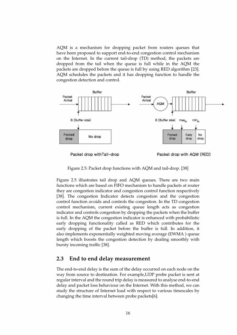
AQM is a mechanism for dropping packet from routers queues thathave been proposed to support end-to-end congestion control mechanismon the Internet. In the current tail-drop (TD) method, the packets aredropped from the tail when the queue is full while in the AQM thepackets are dropped before the queue is full by using RED algorithm [23].AQM schedules the packets and it has dropping function to handle thecongestion detection and control.

Figure 2.5: Packet drop functions with AQM and tail-drop. [38]

Figure 2.5 illustrates tail drop and AQM queues. There are two mainfunctions which are based on FIFO mechanism to handle packets at routerthey are congestion indicator and congestion control function respectively[38]. The congestion Indicator detects congestion and the congestioncontrol function avoids and controls the congestion. In the TD congestioncontrol mechanism, current existing queue length acts as congestionindicator and controls congestion by dropping the packets when the bufferis full. In the AQM the congestion indicator is enhanced with probabilisticearly dropping functionality called as RED which contributes for theearly dropping of the packet before the buffer is full. In addition, italso implements exponentially weighted moving average (EWMA ) queuelength which boosts the congestion detection by dealing smoothly withbursty incoming traffic [38].

2.3 End to end delay measurement

The end-to-end delay is the sum of the delay occurred on each node on theway from source to destination. For example,UDP probe packet is sent atregular interval and the round trip delay is measured to analyse end-to-enddelay and packet loss behaviour on the Internet. With this method, we canstudy the structure of Internet load with respect to various timescales bychanging the time interval between probe packets[6].

16

Component of the end to end delay

The packet from the source has to be routed through various nodesand routers on the way to the destination. We need to categorise thedelay on the basis of the delay occurred in between these intermediatenode and routers. [8] The end to end delay can be categorised into fourmain types: processing delay, transmission delay, propagation delay andqueuing delay. The time required for processing a packet at each nodeand also prepare for retransmission to the respective node is a processingdelay. The protocol stack, computational power available and link driverare the factors deciding the processing delay. The time needed to transferfrom first to last bit via a communication link is referred as a transmissiondelay. The transmission delay is directly affected by the speed of thecommunication channel. The propagation delay is the time to propagatea bit via communication channel link. It is governed by a travel time ofan electromagnetic wave through a physical channel of the communicationpath and is independent of the actual traffic on the link. While the packettraverses the various node it has to be in the buffer of the routers beforeit is retransmitted. Thus the waiting time in the queue is a queuingdelay[8].

Significance of end to end delay measurement

The one way or round trip delay of a UDP packet had been measured on theInternet. Apart from that, various experiments were conducted to measureTCP delays, losses, and other routing dynamics. These experiments oftenhelp researchers to study the strange behaviour of the Internet. Besidesthat, we can measure the delay distribution on the internet and we canfigure out if the QoS on the Internet is verified or not. We can get vitalideas from experiments to re-dimension to minimise the delay. It is possibleto find the bottleneck links where competing traffic leads to congestionvia end to end delay measurement. The delay along with hop countmeasurement can support researchers while choosing the parameters forthe large-scale simulation and modelling of the Internet [7, 8, 9, 17].

2.4 Performance Bottlenecks

A bottleneck refers to a phenomenon where the performance of a systemis limited because of a resource or an application component. The resourcecan be, CPU, memory, disk ,and Network Interface Card. The bottleneckcomponents are the prime causes of undesirable behaviour and poorperformance of the system. [25].

2.4.1 Types of Bottlenecks

There are mainly two types of bottlenecks which are explained asfollowing.

17

Resource Saturation Bottlenecks

When a system has fully utilised the resource or has crossed a set threshold,the situation is regarded as resource Saturation. The performance of thesystem is deteriorated because of the resource saturation. Different systemresources are bottlenecked differently after resource saturation in thesystem. CPU utilisation around 100% results in a congested queue andhence contributes to growth in latency. If a system reaches the memoryconstrained capacity condition due to limited physical memory or memoryleak in the system, there will be constant paging and swapping resultingloss in performance. Similarly, when a system faces disk saturation, theconstant disk access beyond the available bandwidth will force the newIO request to be in a queue. Network saturation conditions due to fullyutilised bandwidth will affect new traffic by dropping them or delayingtheir processing[24].

Resource Contention Bottlenecks

The system has limited resources such as CPU cycles, IO bandwidth, phys-ical memory, buffers, semaphores, mutexes etc.,however, the applicationprocesses in a multitasking environment will contend for those limited re-sources and lead to a performance bottleneck. The most appropriate ex-ample is resource contention among different cloud tenants in cloud datacentres. The contention for different system resources has a distinguishingimpact on performance degradation of the system. The contention for CPUamong multiple process results to congested queue and performance inter-ference especially, in a virtualised system, using CPU hogging programs.Memory contention also has a severe impact on performance. In the sameway, disk contention among processes will cause the performance loss es-pecially, in IO loads because of the performance gap between Processorand IO with restricted disk payload. Network contention will also resultin deterioration of the performance by demanding more communicationlinks at the peak times and hence lowering the effective offered bandwidth[24].

2.4.2 Bottlenecks behaviours

The bottlenecks behaviour is different for the different system an appli-cation. This is governed by the interaction between components and thesystem. Basically, there are three kinds of bottlenecks behaviours.

Single Bottlenecks

The Bottlenecks in a system is because of the predominant saturation ofresource at a single point or component of a system.

18

Multiple Bottlenecks

Two or more than two components of the systems get saturated and simul-taneously contributes for the bottlenecks in the system.This may happenbecause of the interdependency of the components on the system.

Shifting Bottlenecks

This is a little bit complicated issue where the bottleneck shifts fromone component to another or from one point on the system to anotherpoint. This happens because of interdependency between components. Oneapplication may cause another application to change its behaviour and thuschanging the behaviour of the application shifts the bottleneck from onecomponent to another and so on.[25]

2.5 Network Performance Metrics

In order to gain insight into network performance and know its behaviours,we need to measure it. There are several standards and non-standardmetrics available for measurement. In this project, we will use some ofthe well-known metrics such as latency, loss etc. The brief overview of thenetwork metrics is explained as follows.

Availability

Availability metrics evaluates the reliability of the network which meansthe percentage of the time the network is running without failure.

Loss

The loss metrics assess the percentage of packets lost because of thenetwork congestion or transmission error. The loss can be measured forone-way path or two-way path depending on the requirement.

Delay

The delay is a measurement of the time that a packet takes to reach thedestination from the sender. On the basis of the routing path, it can beRound trip time or just in a single path called one-way delay.

Bandwidth

Bandwidth is the amount of data which can be transferred in the networkin a time unit, both dependent and independent from the current networktraffic.Apart from those performance metrics, we need to look for other non-standard metrics which are often related to the system and can contributeto the performance degradation of the network. Thus, monitoring systemresources such as CPU,memory, and load in the network provides the

19

systems overview and resource status. In this way, we will not be misledby the result in case the system is causing the trouble for performancedeterioration.[34]

2.6 PlanetLab Testbed

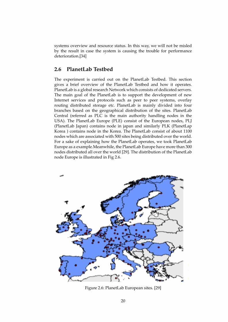
The experiment is carried out on the PlanetLab Testbed. This sectiongives a brief overview of the PlanetLab Testbed and how it operates.PlanetLab is a global research Network which consists of dedicated servers.The main goal of the PlanetLab is to support the development of newInternet services and protocols such as peer to peer systems, overlayrouting distributed storage etc. PlanetLab is mainly divided into fourbranches based on the geographical distribution of the sites. PlanetLabCentral (referred as PLC is the main authority handling nodes in theUSA). The PlanetLab Europe (PLE) consist of the European nodes, PLJ(PlanetLab Japan) contains node in japan and similarly PLK (PlanetLapKorea ) contains node in the Korea. The PlanetLab consist of about 1100nodes which are associated with 500 sites being distributed over the world.For a sake of explaining how the PlanetLab operates, we took PlanetLabEurope as a example.Meanwhile, the PlanetLab Europe have more than 300nodes distributed all over the world [29]. The distribution of the PlanetLabnode Europe is illustrated in Fig 2.6.

Figure 2.6: PlanetLab European sites. [29]

20

PlanetLab nodes are gathered into a set called a slice. Administrator on thebasis of the user’s requests creates the slices. The node in the slice runs aLinux virtual machine referred to as silver. The user can login remotelyto these nodes and run services for experimental purpose. Nodes fromdifferent sites can be added to a slice,therefore same nodes are added todifferent slices and running at the same time. The PlanetLab creates a newsilver and runs on the node thus giving impression that silver as a node forusers.The PlanetLab slice indeed is a collection of the distributed resources.[12]Virtual Machine runs on a single node and allocates the certain portion ofthe resource of the node thus slice can be also the network of the VirtualMachines. Multiple numbers of Virtual Machines run on a PlanetLab nodeand thus there is a VMM to manage the resource sharing among theseVMs at that node. It is interesting to know how the slices are createddynamically and resources are distributed and managed among them.There are 5 components that take control over the process of acquiringslice and resource management. The first component is node manager,which acts partly as VMM in the node. It takes tickets as inputs andchecks if the request can be redeemed. If the request can be fulfilled itreserves the resource and create a VM that takes the reserved resourceand finally replied with leased status. The second component is theresource monitor, which monitors resource periodically and reports tothe agent about the resource availability. In figure 2.7, the steps whileacquiring the slice are depicted, the first step is resource monitoring andreporting resource availability to the agent a third component which isresponsible for advertising the resource availability and requirements tothe tickets.

Figure 2.7: The process of acquiring the slice [12]

21

The fourth component is resource broker, which replies the queries ofthe service manager. The service manager is the fifth component that isassociated with each service, and it contacts a resource broker to find slicespecification and tickets to run it.The query from service manager describesthe resource need to run the service and the principal behind the requestfor service. At step 2, the resource broker contact agent for the descriptionof the ticket that is held by agents for a service. Then the agent respondswith sets of advertisements. The broker combines the advertisements withknown service requirement in order to generate the specification of theslice. Then broker requests for the ticket to instantiate the slice, and agentreplies with the ticket. These phenomena are depicted as steps 3 and 4while acquiring slice. Finally, at step 5, service provides the tickets toadmission control on each node to create a network of virtual machines.When the virtual machines are created then service manager loads andstarts a program in every virtual machine. The admission control returnsthe status lease on the slice.

22

Related Works

One of the latest work was done on inferring congestion on the inter-domain link. The simple and lightweight method called Time SequenceLatency Probes (TSLP). The idea behind this method is to frequently repeatthe Round Trip Time (RTT) measurements from a vantage point to nearand far routers of the inter-domain link where measured RTTs being afunction of the queue length between two routers. The main advantageof the method is that it tries to localize the congestion from a single point,Vantage Point (VP), without a need of responding server on the other end.However, if the experiment produces broadband performance map, it isrequired to have many VP on the several access points. The experimentalresults value proves that it can localise the congestion on the inter-domainlink at the edge. On the course of the experiment, there are many challengeson inferring the inter-domain link and congestion. The challenges arosebecause of the inconsistent numbering conventions as the router mayhave IP interface coming from third party ASes. More precisely the majorchallenges are i) identifying congestion on links with AQM and WFQ ii)proving the response from the far router returns over the targeted inter-domain links iii) ICMP queuing behavior[32].On another related work, a lightweight single end active probing tool calledpathneck was developed which is based on a probing technique known asRecursive Packet Train (RPT). This tool facilitates the end user to locatebottleneck links on the Internet efficiently. The key idea behind RPT isthat it combines load packet and measurement packet in a single packettrain. The load packets are queued at router interface and the trend of thepacket train length is changed and the help of the measurement packetsmeasures the change in the packet train length. In this way by measuringthe packet train length, the location of congestion can be inferred. The resultof the experiment suggests that more than half of the bottleneck locationswere found in the Intra-AS link which is contrary to the widely believedassumption that bottlenecks often occurs at the edge of the network or atthe boundary between the ASes. The stability of the Internet bottleneck wasalso investigated and found that intra-AS bottlenecks are more stable thaninter-AS bottlenecks[22].With the availability of pathneck to infer the bottleneck on the Internet, thedetailed measurement studies were conducted on the Internet bottlenecks.The main four aspects of the Internet bottleneck were investigated. Firstlythe persistence of the Internet bottleneck was checked; secondly, thesharing of the bottleneck among the destination cluster was examined.

23

Besides that the correlation of the bottlenecks with link loss and delayand the relationship to routing properties and link capacity including therouter CPU and link capacity and traffic load were studied. The experimentrevealed that 60% of the bottlenecks on loss paths could be correlatedwith a loss point no more than 2 hops away. There is no strong relationbetween bottleneck and the routing CPU, link capacity memory usagewhereas the traffic load has strong relation with bottleneck occurrence onthe internet.[21]There have been done a lot of works on locating bottlenecks in the network.One of the approaches is locating last-mile downstream throughputbottlenecks. The main contribution of the paper was to identify whetherthe throughput bottlenecks lies inside the home networks or in theiraccess ISPS. In order to facilitate the task, an algorithm was developedwhich finds out the throughput bottlenecks by monitoring traffic flowsbetween home networks and access networks. The lightweight networkmetrics namely Packet Inter-arrival Time and TCP RTT were identified forthe experiment. To validate the algorithm the experiment was conductedon 2652 home across the United States. The experiment revealed thatwireless bottlenecks are more common than access-link bottlenecks whenthe downstream is greater than 20 Mbps. On the other hand, there is alsoaccess-link bottlenecks if the downstream speed is less than 10Mbps inconjunction with at least one device in a home network contributing tothe throughput bottlenecks. There were some limitation of this project.The experiment is based on passive traffic analysis. It cannot detect thebottlenecks that are far away from the last-mile network. This is applicableonly for finding downstream throughput bottlenecks and cannot detect theupstream throughput bottlenecks [3].End-to-End delay is a very prominent performance metrics for studyingand investigating network performance bottlenecks. Delay on the one bot-tleneck link can have a severe effect on the overall performance of the net-work. One of the research has been conducted to investigate the bottleneckdelays and find the geographical distribution of the bottleneck links caus-ing delay. The main contribution of the research is to identify the delaysat the bottleneck links and study the delay feature on the internet whichcan be beneficial for designing the efficient distributed algorithms. In theproject, the measured probing data has been deployed for conducting thestatistical analysis of relationship between one-way delay and bottleneckdelay. The experiment has demonstrated that bottleneck appears in the 70%of the paths on the Internet. Apart from this, for more analysis on bottle-neck delay, the scheme which combines the IP centralised mapping withIP geographical mapping was proposed. In addition, that mapping schemeis handy to calculate link delay on the Internet and analyse the relation-ship between link delay and features of Internet links such as the structureof the internet and geographical distribution. The experiment has demon-strated that the links which had a greater number of entrances( in-degrees) but a smaller number of exit (out-degrees) or the average shallower linksare the culprits for the bottleneck-delay and the two end of the bottlenecklinks are mainly distributed in the same country. The further more analysis

24

on the bottleneck links mapped in the same country has also revealed thatthe main cause of the delay in the bottleneck links is queuing delay.Thus,the paper has revealed how the structural properties of the Internet canmake an impact on the transmission of the internet traffic and contribute togreater end-to-end delay [31].

25

26

Part II

The project

27

2.7 Overview of the project

The goal of this project is to examine congestion in the network whichis limiting the performance of the network. The network is comprisedof the core-network and edge. The general convention is that there is aproblem at the edge which causes the performance degradation. So thesiswill investigate if congestion usually happens in the last mile networkor in the core as well. In order to locate congestion in the network, wehave designed the experimental setup in the PlanetLab Testbed which isexplained in detail in the coming section. The basic idea is to send thepackets between nodes which lie on different domains and record RoundTrip Time and also record the loss among those link. More precisely, we willform inter-domain links by picking up the nodes on the PlanetLab Testbed.We will attempt to maximize the number of the inter-domain link as far aspossible and investigate if there is congestion on those links or not. We willattempt to find the reasons behind the congestion on these inter-domainlinks. The detailed explanation of the experimental design and relevantprocedures and tools are explained in the respective sections.

29

30

Chapter 3

Experiments design andsetup

Figure 3.1 represents a general overview of the experimental designwhere main building blocks of experiments are shown precisely. We havepresented 3 components namely PlanetLab testbed, shell scripts and toolsin 3 separate boxes as the main components of the experiment. ThePlanetLab Testbed is used as Testbed for experiments and all availablenodes of it will take part in the experiment. First of all available nodes arefound out. After that, nodes are filtered such that they should belong todifferent cities and autonomous systems. The idea is to find the maximumnumber of the inter-domain links between nodes having most hops as faras possible. On this course, each node is assigned another 5 nodes thatit will probe . Here the important assumption is that there should notbe duplicate links just by interchanging senders and receiver role ratherall links should be unique. A detailed description of selecting nodes andnode pair is presented in Experiment details section below. All the scriptsand tools that are devised for the experiment are supposed to run on thePlanetLab nodes. To automate operations on the PlanetLab nodes, shellscripts are required and therefore it is regarded as one of the buildingblocks of the experimental design. Basically, a master shell script is usedto login to all nodes and prepare everything and copy the scripts andprogramming codes that are required to run the experiment. The othershell scripts run respectively after master scripts on respective probing andprobed nodes to facilitate the automation over there. Few tools will be alsoused in the experiment which are shown in the box labeled as tools. One ofthe tool is the round-trip time calculating c programming code which sendsthe packets along with sequence number records the sending and receivingtime of the packet and thus calculates the RTT of the packets. Tracerouteis a handy tool to probe nodes and get RTT for each hop. High resourceconsumption such high usage of CPU and memory can sometimes resultin an increased delay. So, to make sure that the larger RTT value is not theimpact of the high resource consumption of the memory and CPU at theparticular node. We are using the tool like top to keep track of the resourceconsumption at the PlanetLab node.

31

Figure 3.1: Overview of the component of experiment.

Figure 3.2 depicts the flow of the experiment more precisely. The systematicsteps and the processes carried out during the experiment are displayed inthe flow chart. In diagram two spots is shown separately. One is PlanetLabtestbed and another one is the computer used to conduct the experimentand communicate with PlanetLab nodes and via which the automationis performed in the testbed. Moreover, in flow chart we depicted theinteraction of the components mentioned in figure 3.1.

3.1 Description and Procedure of Experiment

In this section, we describe the Experiment thoroughly. A detail explana-tion of the entities involved in the experiment will be covered. In addition,we attempt to make the experiment more clear by explaining the experi-mental procedures as well.

3.1.1 Overview of the PlanetLab nodes involved in the Experi-ment

In the PlanetLab testbed, there are many nodes among them nodes wereunreliable so we dropped them out. Besides that, some nodes have firewallsor some other functionalities which prevented us from reaching them. Thebest nodes that were selected for the experiment are listed in table 3.1. Weselected 54 nodes where 23 nodes are from North America, 2 nodes are fromBrazil, 20 nodes are from Europe and 9 nodes from Asia and Australia. Thetable highlights most relevant information about nodes such as geographyalong with the ISP and Autonomous system number.

32

Figure 3.2: The Flow chart for Experiment.

3.1.2 Hardware and System Information

All nodes run Linux. Most of the machines have Fedora (Linux) andsome of them also have CentOS. More precisely, CentOS release 6.4(Final),CentOS release 6.8 (Final),Fedora release 14 (Laughlin),Fedorarelease 8 (Werewolf) Linux distribution are deployed on PlanetLab nodes.The nodes have different hardware, for example, they have differentnumbers of processors with varying number of CPU cores and capacity.Most of the processors use hyper threading functionality as well.Thenumber of processors varies from 2 processors to 16 processors. Then thenumber of CPU cores in each processor varies from 2 CPU cores to 8 CPUcores. The capacity of CPU varies from 2.4GHz to 3.6GHz. Most of thenodes have 4GB of RAM. The disk quota on each node is 9.6GB however insome nodes it varies from several Gigabytes to Terabytes.

3.1.3 Experiments details

Selection of Nodes for experiment

In the PlanetLab website, we can see more than 300 nodes are available.However, the information is not up to date as most of the nodes aredead or unreachable. Therefore, the first step was to find all the nodes

33

SN Nodes ASN/Location country1 mars.planetlab.haw-hamburg.de AS680 DFN Verein zur Foerderung eines Deutschen Forschungsnetzes Germany2 merkur.planetlab.haw-hamburg.de AS680 DFN Verein zur Foerderung eines Deutschen Forschungsnetzes Germany3 node2.planetlab.mathcs.emory.edu AS3512 Emory University United States4 pl1.cs.montana.edu AS13476 Montana State University United States5 pl1.eng.monash.edu.au AS56132 Monash University Australia6 pl1.ucs.indiana.edu AS87 Indiana University United States7 pl2.6test.edu.cn AS23910 China Next Generation Internet CERNET2 China8 pl2.pku.edu.cn AS4538 China Education and Research Network Center China9 pl2.ucs.indiana.edu AS87 Indiana University United States10 plab1.cs.msu.ru AS2848 MSU Vorobjovy Gory, Moscow, Russia Russian Federation11 planet-lab-node1.netgroup.uniroma2.it AS137 ASGARR Consortium GARR Italy12 planet1.pnl.nitech.ac.jp AS2907 Research Organization of Information and Systems, National Japan13 planet2.pnl.nitech.ac.jp AS2907 Research Organization of Information and Systems, National Japan14 planetlab-2.cse.ohio-state.edu AS159 The Ohio State University United States15 planetlab-5.eecs.cwru.edu AS32666 Case Western Reserve University United States16 planetlab-coffee.ait.ie AS1213 HEANET Ireland17 planetlab-js1.cert.org.cn AS4134 Chinanet China18 planetlab-js2.cert.org.cn AS4134 Chinanet China19 planetlab02.cs.washington.edu AS73 University of Washington United States20 planetlab04.cs.washington.edu AS73 University of Washington United States21 planetlab1.cesnet.cz AS2852 CESNET2 Czech Republic22 planetlab1.cs.du.edu AS14041 University Corporation for Atmospheric Research United States23 planetlab1.cs.okstate.edu AS5078 Oklahoma Network for Education Enrichment and United States24 planetlab1.cs.otago.ac.nz AS38305 The University of Otago New Zealand25 planetlab1.dtc.umn.edu AS57 University of Minnesota United States26 planetlab1.ifi.uio.no AS224 UNINETT UNINETT, The Norwegian University and Research Norway27 planetlab1.net.in.tum.de AS12816 MWN-AS Germany28 planetlab1.pop-mg.rnp.br AS1916 Associacao Rede Nacional de Ensino e Pesquisa Brazil29 planetlab1.unr.edu AS3851 Nevada System of Higher Education United States30 planetlab1.virtues.fi AS47605 FNE-AS Finland31 planetlab2.cesnet.cz AS2852 CESNET2 Czech Republic32 planetlab2.citadel.edu AS53257 The Citadel United States33 planetlab2.cs.cornell.edu AS26 Cornell University United States34 planetlab2.cs.du.edu AS14041 University Corporation for Atmospheric Research United States35 planetlab2.cs.otago.ac.nz AS38305 The University of Otago New Zealand36 planetlab2.cs.ubc.ca AS393249 University of British Columbia Canada37 planetlab2.cs.uoregon.edu AS3582 University of Oregon United States38 planetlab2.inf.ethz.ch AS559 SWITCH Peering requests: <[email protected]> Switzerland39 planetlab2.pop-mg.rnp.br AS1916 Associacao Rede Nacional de Ensino e Pesquisa Brazil40 planetlab2.rutgers.edu AS46 Rutgers University United States41 planetlab2.tlm.unavarra.es AS766 REDIRIS RedIRIS Autonomous System Spain42 planetlab2.utdallas.edu AS20162 University of Texas at Dallas United States43 planetlab2.utt.fr AS2200 Reseau National de telecommunications pour la Technologie France44 planetlab3.cesnet.cz AS2852 CESNET2 Czech Republic45 planetlab3.cs.uoregon.edu AS3582 University of Oregon United States46 planetlab3.eecs.umich.edu AS36375 University of Michigan United States47 planetlab3.inf.ethz.ch AS559 SWITCH Peering requests: <[email protected]> Switzerland48 planetlab3.mini.pw.edu.pl AS12464 PW-NET Poland49 planetlab4.inf.ethz.ch AS559 SWITCH Peering requests: <[email protected]> Switzerland50 planetlab4.mini.pw.edu.pl AS12464 PW-NET Poland51 planetlab5.eecs.umich.edu AS36375 University of Michigan United States52 ple2.cesnet.cz AS2852 CESNET2 Czech Republic53 salt.planetlab.cs.umd.edu AS27 University of Maryland United States54 stella.planetlab.ntua.gr AS3323 NTUA Greece

Table 3.1: List of PlanetLab nodes with location information

that are accessible. After getting a list of accessible nodes we checked thefunctionalities and programs that are required for running the experimentare available or not. If the program and service are lacking then we tried toinstall them manually. We tried to fix minor issues like repository errors,DNS error,etc. Thereafter we begin filtering the nodes by dropping thenodes which can not be maintained for running the experiment. In theprocess of selecting nodes, we got around 70 available nodes and afterdropping the nodes which are unreliable. Thus,we end up with 54 suitablenodes for conducting experiments.

Selection of Node pairs

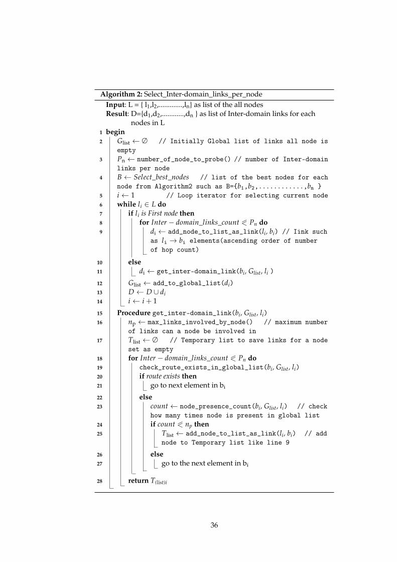
After getting a list of suitable PlanetLab nodes the next task is togenerate the inter-domain links from them for each node. The task carriedout by applying two algorithms shown in Algorithm1 and Algorithm2

34

respectively. Here, we have used a term inter-domain links for node pairswhich are from different networks.

Algorithm 1: Select_best_nodesInput: L = { l1,l2,.............,ln} as list of the all nodesResult: B={b1,b2,............,bn } as list of Best nodes for each nodes in L

1 begin2 B← ∅ // Empty set initialisation3 i← 1 // Loop iterator for selecting current node4 while li ∈ L do5 bi ← get_best_node(li, L)6 B← B ∪ bi7 i← i + 1

8 Procedure get_best_node(li, L)9 l(Hop)i ← trace_route_all(li, L) // List of nodes with

number of hop count10 l(City_AS)i ← get_city_and_AS(l(Hop)i, L) // List of nodes

with AS,City, hop count11 l(Sorted_City_AS)i ← get_unique_AS_and_city(l(City_AS)i, L)

// filtered and sorted by unique city and AS count12 l(Final)i ← sort_nodes_by_hop_count(l(Sorted_City_AS)i)

// Final filtered and sorted by hop count list13 return l(Final)i

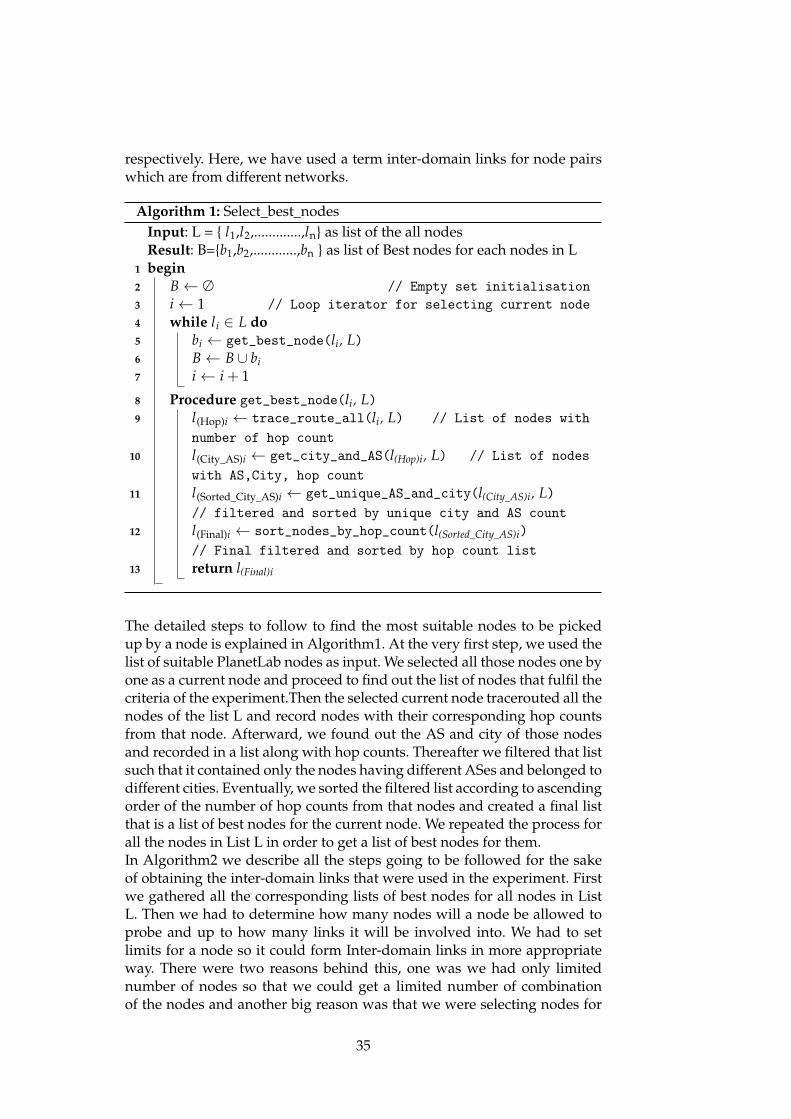
The detailed steps to follow to find the most suitable nodes to be pickedup by a node is explained in Algorithm1. At the very first step, we used thelist of suitable PlanetLab nodes as input. We selected all those nodes one byone as a current node and proceed to find out the list of nodes that fulfil thecriteria of the experiment.Then the selected current node tracerouted all thenodes of the list L and record nodes with their corresponding hop countsfrom that node. Afterward, we found out the AS and city of those nodesand recorded in a list along with hop counts. Thereafter we filtered that listsuch that it contained only the nodes having different ASes and belonged todifferent cities. Eventually, we sorted the filtered list according to ascendingorder of the number of hop counts from that nodes and created a final listthat is a list of best nodes for the current node. We repeated the process forall the nodes in List L in order to get a list of best nodes for them.In Algorithm2 we describe all the steps going to be followed for the sakeof obtaining the inter-domain links that were used in the experiment. Firstwe gathered all the corresponding lists of best nodes for all nodes in ListL. Then we had to determine how many nodes will a node be allowed toprobe and up to how many links it will be involved into. We had to setlimits for a node so it could form Inter-domain links in more appropriateway. There were two reasons behind this, one was we had only limitednumber of nodes so that we could get a limited number of combinationof the nodes and another big reason was that we were selecting nodes for

35

Algorithm 2: Select_Inter-domain_links_per_nodeInput: L = { l1,l2,.............,ln} as list of the all nodesResult: D={d1,d2,............,dn } as list of Inter-domain links for each

nodes in L1 begin2 Glist ← ∅ // Initially Global list of links all node is

empty3 Pn ← number_of_node_to_probe() // number of Inter-domain

links per node4 B← Select_best_nodes // list of the best nodes for each

node from Algorithm2 such as B={b1,b2,............,bn }5 i← 1 // Loop iterator for selecting current node6 while li ∈ L do7 if li is First node then8 for Inter− domain_links_count 0 Pn do9 di ← add_node_to_list_as_link(li, bi) // Iink such

as li → bi elements(ascending order of numberof hop count)

10 else11 di ← get_inter-domain_link(bi, Glist, li )

12 Glist ← add_to_global_list(di)13 D ← D ∪ di14 i← i + 1

15 Procedure get_inter-domain_link(bi, Glist, li)16 np ← max_links_involved_by_node() // maximum number

of links can a node be involved in17 Tlist ← ∅ // Temporary list to save links for a node

set as empty18 for Inter− domain_links_count 0 Pn do19 check_route_exists_in_global_list(bi, Glist, li)20 if route exists then21 go to next element in bi

22 else23 count← node_presence_count(bi, Glist, li) // check

how many times node is present in global list24 if count 0 np then25 Tlist ← add_node_to_list_as_link(li, bi) // add

node to Temporary list like line 9

26 else27 go to the next element in bi

28 return T(list)i

36

inter-domain links from the lists where node were sorted according to hopcounts. Hence for each node, we tried to find the farthest nodes as far aspossible. Therefore, if we did not limit the presence of the node on theprocess farthest node will be probed several times and closet nodes willbe probed rarely. Then we began to find inter-domain links for each nodesequentially. If a node currently being processed was a first node of thelist then we simply added nodes maintaining limitation from its list of bestnodes to the list of its inter-domain links. Subsequently, we added to theglobal list which will be used to check for the presence of duplicate linksfor coming up nodes. For other nodes, we need to check in the global listof inter-domain links for the avoidance of duplicate links and at the sametime, we would be checking how many the nodes were involved in formingthe links as well. Thereafter, if the link satisfied both criteria, we added itto the list of the corresponding node and then to the global list respectively.This process was repeated util we got the list of inter-domain links for allthe nodes in the set L.

Development of Programs and Scripts

To measure Latency, we designed a C program that sends packets to thelist of the nodes and receives back from them. To measure the RoundTrip Time the sending and receiving timestamp were logged in separatefiles. Similarly, we designed the shell scripts that monitors the load in thesystem and traceroutes from sender to receiver and vice versa. In addition,a python script was created to calculate the RTT and loss between links.A separate script to collect the data every day via cronjob was prepared.Besides that reformatting and arranging data was done via other scriptsas well. In general, we created several scripts for individual purposeand combined all to 2 parts one for running experiments and collectingdata and other for rearranging and reformatting the collected data as perrequirements

Running experiment

we set up a separate Laptop computer for running the experiments andcollecting data. The experiment was run as a cronjob which runs everyweek. The experiment was arranged to run for 3 weeks.The experiments began with the main shell scripts which prepared all therequirement for running other programs by installing required services andcopying all the relevant file to the respective nodes. Basically, we coulddivide the experimental task into 3 different tasks as following.Probing nodes with packets : We ran a C code to probe node by sendingpackets from one end of the link to the node on the another end. Onenode acted as a sender and sent the packet to receiving node meanwhileanother C code was running on the receiving side to receive packets andsend back the same packet to the sender. We created two separate thread forsending the packet and receiving packet so that the sending and receivingtask are independent and do not interfere with each other. We had also set

37

the sending rate such as we sent the packet every 200ms. We logged thetimestamp and sequence number of the packet on both the sending andthe receiving end of the link.Tracerouting the nodes: While we were probing nodes by sendingthe packets, we were also tracerouting the nodes. More precisely, wetracerouted in a two-way fashion from sender to receiver and receiver tosender at the same time. We logged the timestamp when we traceroutedand output of traceroute.Monitoring resource and the load in the node: During the experiment, wealso kept track of resource consumption and load on the nodes. We used topcommand to check the CPU utilization, memory consumption, I/O waitingand average load on the node. The main purpose of the monitoring thenode was to confirm that if there is congestion on the particular link thenthe load and resource on the node are not culprits on that context.

Data Collection

The data was collected every day from remote PlanetLab nodes to a locallaptop by running a script as a cronjob. We collected data every day be-cause of two reasons 1)We could use data every day for analysis and didnot need to wait for the experiment to be completed. 2) The disk on the re-mote server has a limited quota and we can get rid of disk quota exceededproblem.

The detail steps involved for collecting the results from remote server tolocal computer is mentioned on Algorithm 3. First of the file to be collectedis identified thereafter those are located.The located files are copied to newfiles respectively so that we do not loose the data in between the copyingprocess. Then the files are compressed and sent to the local computer. Ifthe files are successfully transferred, then we just delete them in order tomaintain free disk space at the nodes.

Data Rearrangement

After completion of data collection task, we need to arrange the data inmore appropriate away for future access. First of all, we uncompress allthe data and then we selected the desired file. Afterward, we merged thecorresponding files into a single file.Thereafter we saved those files to anew path in such a way we can recognise the files belongs to which linksand in which direction of the links. The figure 3.3 below gives a moreclear image about this. All the nodes that have been probed are put underprobed_nodes folder along with all the log files. The nodes which probed anode are put under probing_nodes folder along with all corresponding logfiles.

38

Algorithm 3: Collect_data_Every dayInput: L = { l1,l2,.............,ln} as list of the all nodesResult: R={r1,r2,............,rn } as zipped data from each nodes in L

1 begin2 R← ∅ // Empty set initialisation3 File =

{sending_packet_log, receivining_packet_log, traceroute_log, top_log}// list of files to collect

4 i← 1 // Loop iterator for selecting current node5 while li ∈ L do6 ri ← get_data_from_remotenode(li, File)7 R← R ∪ ri8 i← i + 1

9 Procedure get_data_from_remotenode(li, File)10 Filerotation =

{sending_packet_lognew,receivining_packet_lognew,traceroute_lognew,top_lognew}// original files rotated to new log files

11 locate_required_logfile( File)Filerotation ← rotate_located_file(File) // rotate fileto new supplied file names respectively

12 Filecompressed ← compress_rotated_files(Filerotation)// compress files after log rotation

13 return Filecompressed

14 delete_compressed_file(Filecompressed)

39

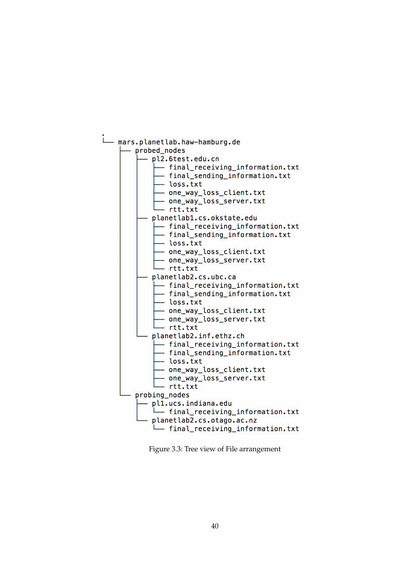
Figure 3.3: Tree view of File arrangement

40

Calculation of Metrics

We calculated the latency by computing Round Trip Time (RTT) for eachpacket. The RTT was computed in microseconds first and then convertedto milliseconds. Besides that, we also calculated loss as another metrics.The loss can be 1)Two-way loss 2) one-way loss from sender to receiver 3)one-way loss from receiver to sender.

41

42

Part III

Analysis and Results

43

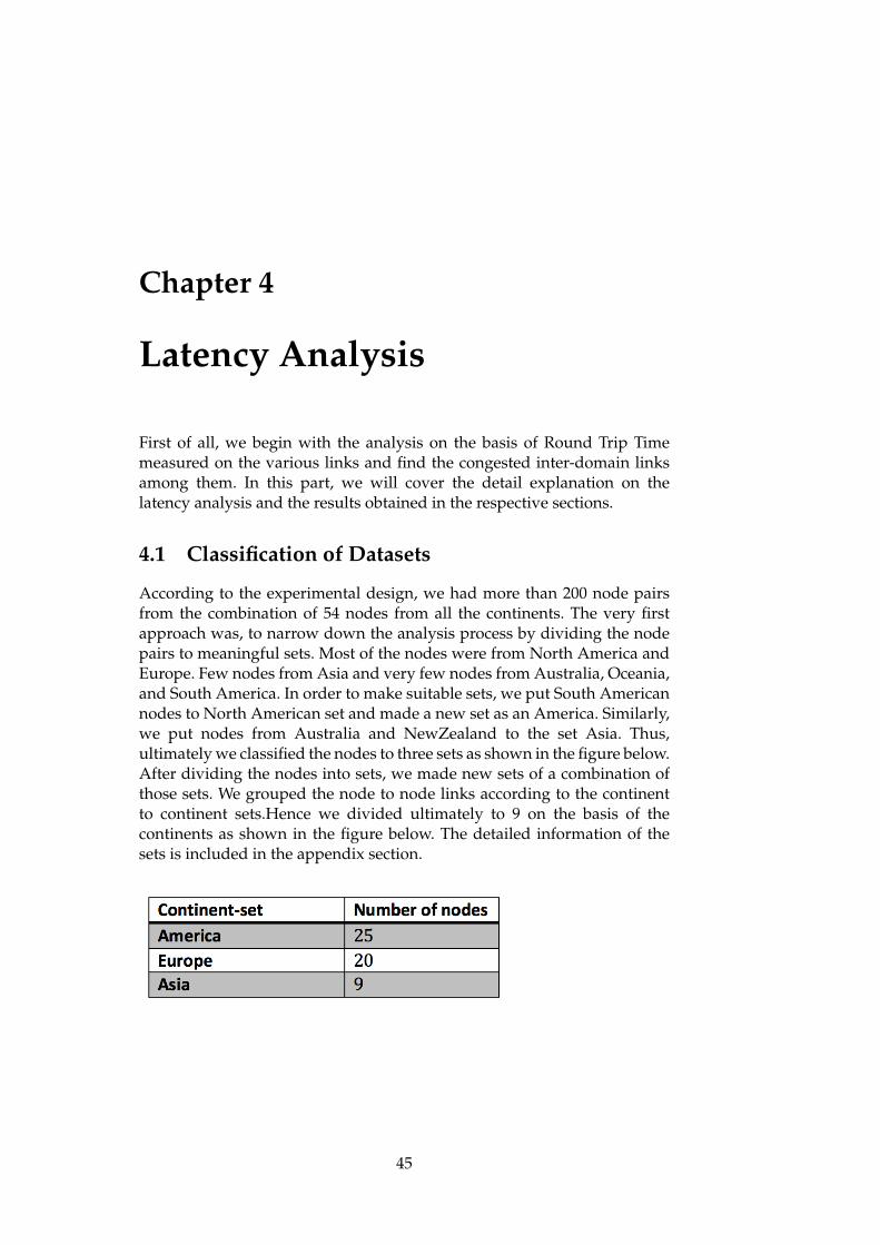
Chapter 4

Latency Analysis

First of all, we begin with the analysis on the basis of Round Trip Timemeasured on the various links and find the congested inter-domain linksamong them. In this part, we will cover the detail explanation on thelatency analysis and the results obtained in the respective sections.

4.1 Classification of Datasets

According to the experimental design, we had more than 200 node pairsfrom the combination of 54 nodes from all the continents. The very firstapproach was, to narrow down the analysis process by dividing the nodepairs to meaningful sets. Most of the nodes were from North America andEurope. Few nodes from Asia and very few nodes from Australia, Oceania,and South America. In order to make suitable sets, we put South Americannodes to North American set and made a new set as an America. Similarly,we put nodes from Australia and NewZealand to the set Asia. Thus,ultimately we classified the nodes to three sets as shown in the figure below.After dividing the nodes into sets, we made new sets of a combination ofthose sets. We grouped the node to node links according to the continentto continent sets.Hence we divided ultimately to 9 on the basis of thecontinents as shown in the figure below. The detailed information of thesets is included in the appendix section.

45

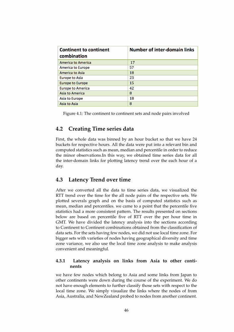
Figure 4.1: The continent to continent sets and node pairs involved

4.2 Creating Time series data

First, the whole data was binned by an hour bucket so that we have 24buckets for respective hours. All the data were put into a relevant bin andcomputed statistics such as mean, median and percentile in order to reducethe minor observations.In this way, we obtained time series data for allthe inter-domain links for plotting latency trend over the each hour of aday.

4.3 Latency Trend over time

After we converted all the data to time series data, we visualized theRTT trend over the time for the all node pairs of the respective sets. Weplotted severals graph and on the basis of computed statistics such asmean, median and percentiles. we came to a point that the percentile fivestatistics had a more consistent pattern. The results presented on sectionsbelow are based on percentile five of RTT over the per hour time inGMT. We have divided the latency analysis into the sections accordingto Continent to Continent combinations obtained from the classification ofdata sets. For the sets having few nodes, we did not use local time zone. Forbigger sets with varieties of nodes having geographical diversity and timezone variance, we also use the local time zone analysis to make analysisconvenient and meaningful.

4.3.1 Latency analysis on links from Asia to other conti-nents

we have few nodes which belong to Asia and some links from Japan toother continents were down during the course of the experiment. We donot have enough elements to further classify those sets with respect to thelocal time zone. We simply visualize the links where the nodes of fromAsia, Australia, and NewZealand probed to nodes from another continent.

46

The aim is to find the hours when the links have peak RTT values and howthe RTT varies over 24 hours. The plots below depicts the RTT trend of thelinks over time from Asia to other continents.

Figure 4.2 pictures the RTT trend of the links from Asia to Europe. Thenodes that are probing to another node are mostly from China and very fewnodes are from Australia and NewZealand. The nodes probed in Europeare distributed all over Europe.One thing clearly noticed in the graph isthat many links have a very high value of the RTT. Different links depicteddifferent RTT trend over 24 hours time. However, we found the hours whenthe links have high RTT values. In the links planetlab-js1.cert.org.cn ->stella.planetlab.ntua.gr, pl1.eng.monash.edu.au ->stella.planetlab.ntua.gr,and planetlab-js1.cert.org.cn ->planetlab1.ifi.uio.no, we can point that thelinks experience RTT fluctuation at hour 5 and also between hours 12 and16.

Figure 4.3 represents the RTT trend of the links from Asia to America. Dur-ing experiment some links were not accessible because the participatingnodes were down as matter of fact we got only 3 links to analyze. Here thenodes from china are probing to nodes in Brazil and the US. In the con-text of the link between china and the US, we did not observe meaningfulvariance on RTT trend. In the link from china to Brazil we noticed two RTTspikes at hour 4 and hour 14.

Figure 4.4 depicts the RTT trend of the links from Asia to Asia set. Thenodes that are probing to another node are from China and a node is fromAustralia. The nodes being are probed belongs to China, Australia, andNewZealand. Here also the nodes from Japan to another country were notaccessible because nodes in Japan went down during the experiment as aconsequence we have fewer links to analyse. From the insight to the graphwe can notice that most of the links don’t show the variation in RTT overtime. One link from Australia to China has variation on RTT trend overtime. The RTT values rises gradually and reaches at peak at hour 14 andafter hour 14 RTT values decreases gradually to a lowest value.

47

330

360

390

420

0 1 2 3 4 5 6 7 8 9 10 11 12 13 14 15 16 17 18 19 20 21 22 23 24

Hours

RT

T (

perc

entil

e_5)

links

planetlab2.cs.otago.ac.nz−> mars.planetlab.haw−hamburg.deplanetlab1.cs.otago.ac.nz−> merkur.planetlab.haw−hamburg.depl2.6test.edu.cn−> plab1.cs.msu.ruplanet1.pnl.nitech.ac.jp−> plab1.cs.msu.ruplanetlab2.cs.otago.ac.nz−> planet−lab−node1.netgroup.uniroma2.itplanetlab−js1.cert.org.cn−> planetlab1.ifi.uio.noplanet1.pnl.nitech.ac.jp−> planetlab1.virtues.fiplanet2.pnl.nitech.ac.jp−> planetlab1.virtues.fiplanetlab−js2.cert.org.cn−> planetlab2.inf.ethz.chplanetlab−js1.cert.org.cn−> planetlab2.tlm.unavarra.esplanetlab1.cs.otago.ac.nz−> planetlab2.utt.frplanetlab2.cs.otago.ac.nz−> planetlab2.utt.frplanetlab1.cs.otago.ac.nz−> planetlab4.inf.ethz.chpl1.eng.monash.edu.au−> stella.planetlab.ntua.grplanetlab−js1.cert.org.cn−> stella.planetlab.ntua.grplanetlab1.cs.otago.ac.nz−> stella.planetlab.ntua.grplanetlab2.cs.otago.ac.nz−> stella.planetlab.ntua.gr

RTT Plot for Asia Australia oceania to Europe

Figure 4.2: Latency trend over hours on the links from Asia to Europe Set

48

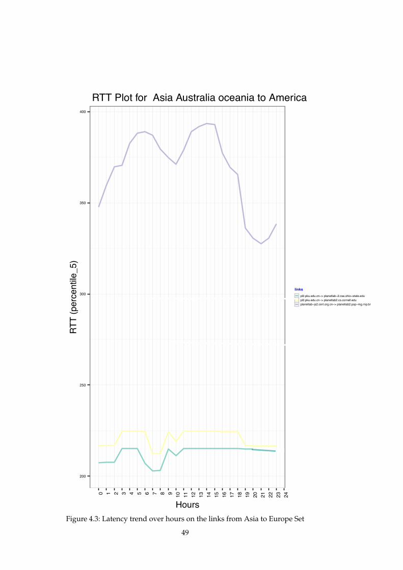
200

250

300

350

400

0 1 2 3 4 5 6 7 8 9 10 11 12 13 14 15 16 17 18 19 20 21 22 23 24

Hours

RTT

(per

cent

ile_5

)

links

pl2.pku.edu.cn−> planetlab−2.cse.ohio−state.edupl2.pku.edu.cn−> planetlab2.cs.cornell.eduplanetlab−js2.cert.org.cn−> planetlab2.pop−mg.rnp.br

RTT Plot for Asia Australia oceania to America

Figure 4.3: Latency trend over hours on the links from Asia to Europe Set

49

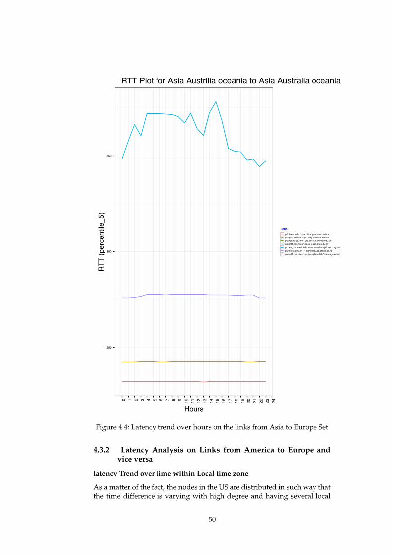
250

300

350

0 1 2 3 4 5 6 7 8 9 10 11 12 13 14 15 16 17 18 19 20 21 22 23 24

Hours

RTT

(per

cent

ile_5

)

links

pl2.6test.edu.cn−> pl1.eng.monash.edu.aupl2.pku.edu.cn−> pl1.eng.monash.edu.auplanetlab−js2.cert.org.cn−> pl2.6test.edu.cnplanet1.pnl.nitech.ac.jp−> pl2.pku.edu.cnpl1.eng.monash.edu.au−> planetlab−js2.cert.org.cnpl2.6test.edu.cn−> planetlab2.cs.otago.ac.nzplanet1.pnl.nitech.ac.jp−> planetlab2.cs.otago.ac.nz

RTT Plot for Asia Austrilia oceania to Asia Australia oceania

Figure 4.4: Latency trend over hours on the links from Asia to Europe Set

4.3.2 Latency Analysis on Links from America to Europe andvice versa

latency Trend over time within Local time zone

As a matter of the fact, the nodes in the US are distributed in such way thatthe time difference is varying with high degree and having several local

50

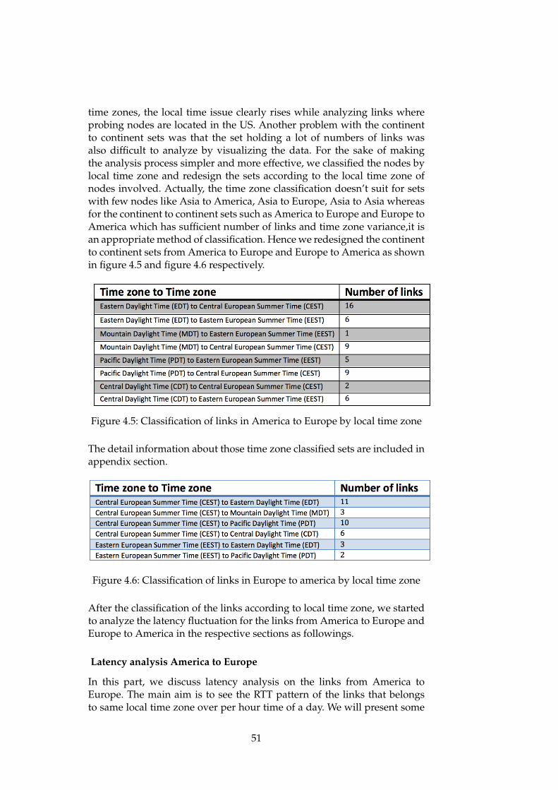
time zones, the local time issue clearly rises while analyzing links whereprobing nodes are located in the US. Another problem with the continentto continent sets was that the set holding a lot of numbers of links wasalso difficult to analyze by visualizing the data. For the sake of makingthe analysis process simpler and more effective, we classified the nodes bylocal time zone and redesign the sets according to the local time zone ofnodes involved. Actually, the time zone classification doesn’t suit for setswith few nodes like Asia to America, Asia to Europe, Asia to Asia whereasfor the continent to continent sets such as America to Europe and Europe toAmerica which has sufficient number of links and time zone variance,it isan appropriate method of classification. Hence we redesigned the continentto continent sets from America to Europe and Europe to America as shownin figure 4.5 and figure 4.6 respectively.

Figure 4.5: Classification of links in America to Europe by local time zone

The detail information about those time zone classified sets are included inappendix section.

Figure 4.6: Classification of links in Europe to america by local time zone

After the classification of the links according to local time zone, we startedto analyze the latency fluctuation for the links from America to Europe andEurope to America in the respective sections as followings.

Latency analysis America to Europe

In this part, we discuss latency analysis on the links from America toEurope. The main aim is to see the RTT pattern of the links that belongsto same local time zone over per hour time of a day. We will present some

51

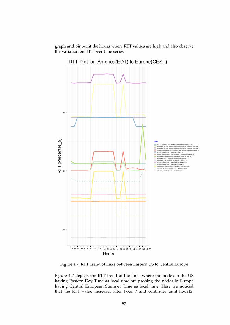
graph and pinpoint the hours where RTT values are high and also observethe variation on RTT over time series.

100

120

140

0 1 2 3 4 5 6 7 8 9 10 11 12 13 14 15 16 17 18 19 20 21 22 23 24

Hours

RT

T (

Per

cent

ile_5

)

links

pl2.ucs.indiana.edu−> merkur.planetlab.haw−hamburg.deplanetlab3.eecs.umich.edu−> planet−lab−node1.netgroup.uniroma2.itplanetlab5.eecs.umich.edu−> planet−lab−node1.netgroup.uniroma2.itsalt.planetlab.cs.umd.edu−> planet−lab−node1.netgroup.uniroma2.itpl1.ucs.indiana.edu−> planetlab1.ifi.uio.nonode2.planetlab.mathcs.emory.edu−> planetlab2.inf.ethz.chplanetlab−2.cse.ohio−state.edu−> planetlab2.inf.ethz.chplanetlab−5.eecs.cwru.edu−> planetlab2.inf.ethz.chplanetlab2.cs.cornell.edu−> planetlab2.inf.ethz.chpl2.ucs.indiana.edu−> planetlab2.tlm.unavarra.espl2.ucs.indiana.edu−> planetlab4.inf.ethz.chnode2.planetlab.mathcs.emory.edu−> ple2.cesnet.czplanetlab−2.cse.ohio−state.edu−> ple2.cesnet.czplanetlab2.cs.cornell.edu−> ple2.cesnet.cz

RTT Plot for America(EDT) to Europe(CEST)

Figure 4.7: RTT Trend of links between Eastern US to Central Europe

Figure 4.7 depicts the RTT trend of the links where the nodes in the UShaving Eastern Day Time as local time are probing the nodes in Europehaving Central European Summer Time as local time. Here we noticedthat the RTT value increases after hour 7 and continues until hour12.

52

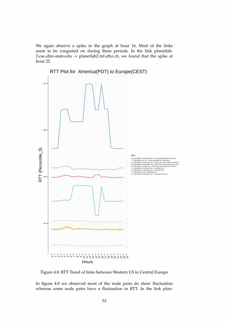
We again observe a spike in the graph at hour 16. Most of the linksseem to be congested on during these periods. In the link planetlab-2.cse.ohio-state.edu -> planetlab2.inf.ethz.ch, we found that the spike athour 22.

160

180

200

220

0 1 2 3 4 5 6 7 8 9 10 11 12 13 14 15 16 17 18 19 20 21 22 23 24

Hours

RT

T (

Per

cent

ile_5

)

links

planetlab04.cs.washington.edu−> merkur.planetlab.haw−hamburg.deplanetlab2.cs.ubc.ca−> merkur.planetlab.haw−hamburg.deplanetlab02.cs.washington.edu−> planet−lab−node1.netgroup.uniroma2.itplanetlab04.cs.washington.edu−> planet−lab−node1.netgroup.uniroma2.itplanetlab2.cs.uoregon.edu−> planet−lab−node1.netgroup.uniroma2.itplanetlab02.cs.washington.edu−> planetlab2.utt.frplanetlab04.cs.washington.edu−> planetlab2.utt.frplanetlab1.unr.edu−> planetlab2.utt.frplanetlab02.cs.washington.edu−> planetlab3.inf.ethz.ch

RTT Plot for America(PDT) to Europe(CEST)

Figure 4.8: RTT Trend of links between Western US to Central Europe

In figure 4.8 we observed most of the node pairs do show fluctuationwhereas some node pairs have a fluctuation in RTT. In the link plan-

53

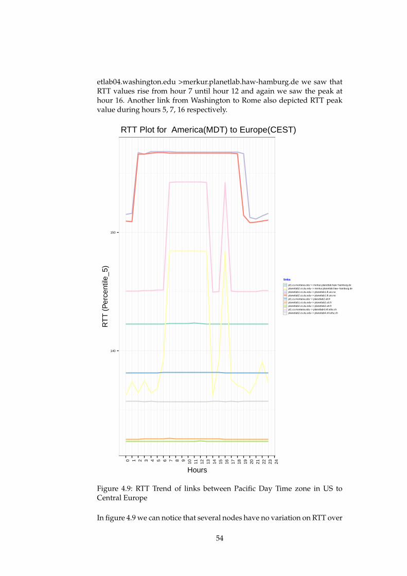
etlab04.washington.edu >merkur.planetlab.haw-hamburg.de we saw thatRTT values rise from hour 7 until hour 12 and again we saw the peak athour 16. Another link from Washington to Rome also depicted RTT peakvalue during hours 5, 7, 16 respectively.

140

150

0 1 2 3 4 5 6 7 8 9 10 11 12 13 14 15 16 17 18 19 20 21 22 23 24

Hours

RT

T (

Per

cent

ile_5

)

links

pl1.cs.montana.edu−> merkur.planetlab.haw−hamburg.deplanetlab2.cs.du.edu−> merkur.planetlab.haw−hamburg.deplanetlab1.cs.du.edu−> planetlab1.ifi.uio.noplanetlab2.cs.du.edu−> planetlab1.ifi.uio.nopl1.cs.montana.edu−> planetlab2.utt.frplanetlab1.cs.du.edu−> planetlab2.utt.frplanetlab2.cs.du.edu−> planetlab2.utt.frpl1.cs.montana.edu−> planetlab4.inf.ethz.chplanetlab2.cs.du.edu−> planetlab4.inf.ethz.ch

RTT Plot for America(MDT) to Europe(CEST)

Figure 4.9: RTT Trend of links between Pacific Day Time zone in US toCentral Europe

In figure 4.9 we can notice that several nodes have no variation on RTT over

54

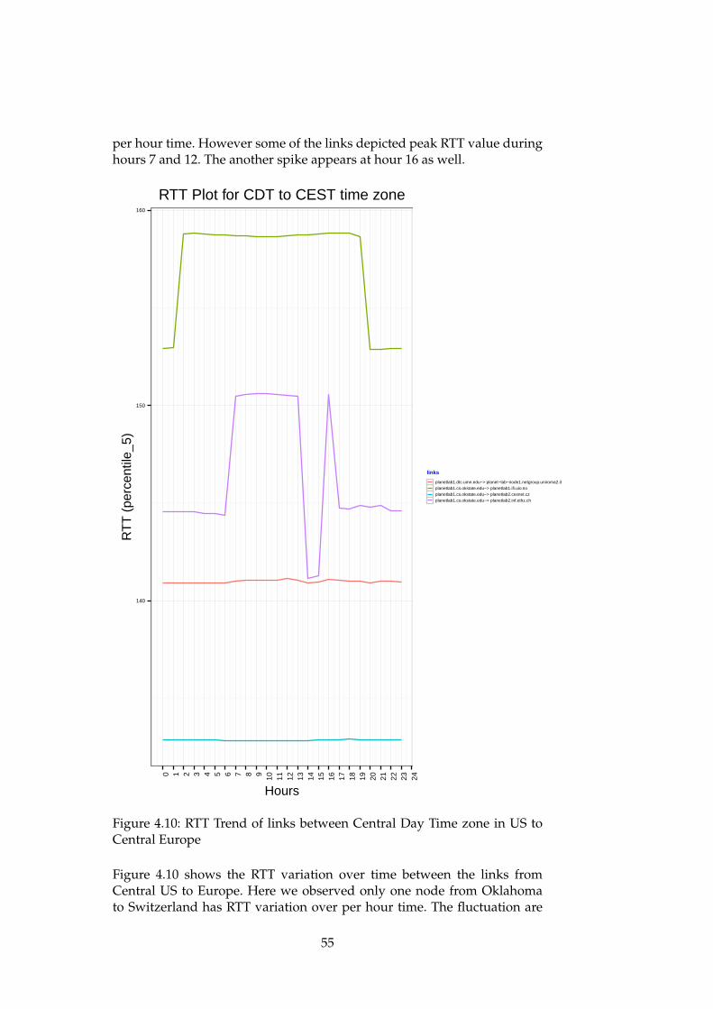
per hour time. However some of the links depicted peak RTT value duringhours 7 and 12. The another spike appears at hour 16 as well.

140

150

160

0 1 2 3 4 5 6 7 8 9 10 11 12 13 14 15 16 17 18 19 20 21 22 23 24

Hours

RT

T (

perc

entil

e_5)

links

planetlab1.dtc.umn.edu−> planet−lab−node1.netgroup.uniroma2.itplanetlab1.cs.okstate.edu−> planetlab1.ifi.uio.noplanetlab1.cs.okstate.edu−> planetlab2.cesnet.czplanetlab1.cs.okstate.edu−> planetlab2.inf.ethz.ch

RTT Plot for CDT to CEST time zone

Figure 4.10: RTT Trend of links between Central Day Time zone in US toCentral Europe

Figure 4.10 shows the RTT variation over time between the links fromCentral US to Europe. Here we observed only one node from Oklahomato Switzerland has RTT variation over per hour time. The fluctuation are

55

observed between period hour 7 to 12 and at hour 16 as well like previouslinks.

180

200

220

240

0 1 2 3 4 5 6 7 8 9 10 11 12 13 14 15 16 17 18 19 20 21 22 23 24

Hours

RT

T (

Per

cent

ile_5

)

links

planetlab2.cs.ubc.ca−> plab1.cs.msu.ruplanetlab2.cs.uoregon.edu−> plab1.cs.msu.ruplanetlab02.cs.washington.edu−> stella.planetlab.ntua.grplanetlab04.cs.washington.edu−> stella.planetlab.ntua.grplanetlab2.cs.uoregon.edu−> stella.planetlab.ntua.gr

RTT Plot for PDT to EEST time zone

Figure 4.11: RTT Trend of links between Pacific Day Time zone in the US toEastern Europe

Figure 4.11 represent the RTT pattern over time between links from PacificDay Time in the US to Eastern Europe. There were few links in EasternEurope as a matter of the fact we have fewer items for analysis on that zone.

56

The links in another time zone of the US did not reflect many variations inRTT observations. However, we noticed slight fluctuation on RTT on twolinks at hour 4 and period between hour 12 and 17.

Latency analysis of links from Europe to America

In this section, we present the result obtained from analyzing the linksfrom Europe to America. We visualize the RTT trend of the links havinga common local time zone and pinpoint the hours where the link has highRTT value. We plotted the graph for all the sets based on the local timezone mentioned in the above section. We will explain most relevant resultamong them as follows. Figure 4.12 shows the RTT trend of the links fromCentral European Summer Time to Central Day Time in the US. The insightto the figure revealed that most of the links have same RTT trend over thetime series while some links remained non-fluctuated. We also noticed thatseveral nodes from Europe probing to only 2 nodes in the US and observedpattern resembles for all with the only difference in the RTT values. TheRTT values started to rise at hour 7 and become steady until hour 12. Afterthat RTT value comes to original trend and again all of sudden the RTTvalue peaks at hour 16.Figure 4.13 depicts the RTT variation on the links from Central EuropeSummer Time to Pacific Day Time in the US. In the figure, we observedthat most of the links have a similar pattern. We can see that RTTvalues don not fluctuate except between hours 20 and 21 where thereis a slight drop in RTT. Apart from this we still noticed that in the linkbetween planetlab3.cesnet.cz and planetlab04.cs.washington.edu there isfluctuation in RTT. The RTT values peak at hour 7 and continues until hour12. After hour 12 the RTT value catches the normal value and all of suddenthe RTT value peaks again at hour 16.We also performed the analysis on the links from Europe to Eastern DayTime and Mountain Day Time. On the process of visualizing the RTTtrend over the time, we did not notice much fluctuation. For instance, wepresented the scenario in figure 4.14 where we see that there is no variationin RTT over time series.

4.3.3 Latency analysis of links from Europe to Asia

In this section, we present the result of analysis on links from Europe toAsia. First, we visualize all links in from Europe to Asia, Australia and,NewZealand as whole in one. After this, we visualize the RTT fluctuationon the links from Europe with local time zone as Central European SummerTime to China separately. In that context,we visualize the RTT trend whiletaking local time zone on consideration since China exercises only one timezone as China Standard Time.

57

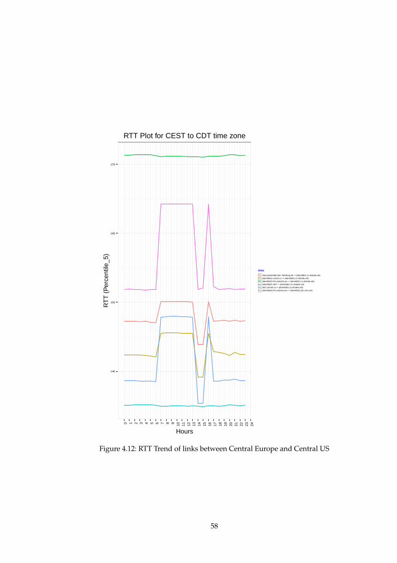
140

150

160

170

0 1 2 3 4 5 6 7 8 9 10 11 12 13 14 15 16 17 18 19 20 21 22 23 24

Hours

RT

T (

Per

cent

ile_5

)

links

mars.planetlab.haw−hamburg.de−> planetlab1.cs.okstate.eduplanetlab1.cesnet.cz−> planetlab1.cs.okstate.eduplanetlab2.tlm.unavarra.es−> planetlab1.cs.okstate.eduplanetlab2.utt.fr−> planetlab1.cs.okstate.eduple2.cesnet.cz−> planetlab1.cs.okstate.eduplanetlab2.tlm.unavarra.es−> planetlab1.dtc.umn.edu

RTT Plot for CEST to CDT time zone

Figure 4.12: RTT Trend of links between Central Europe and Central US

58

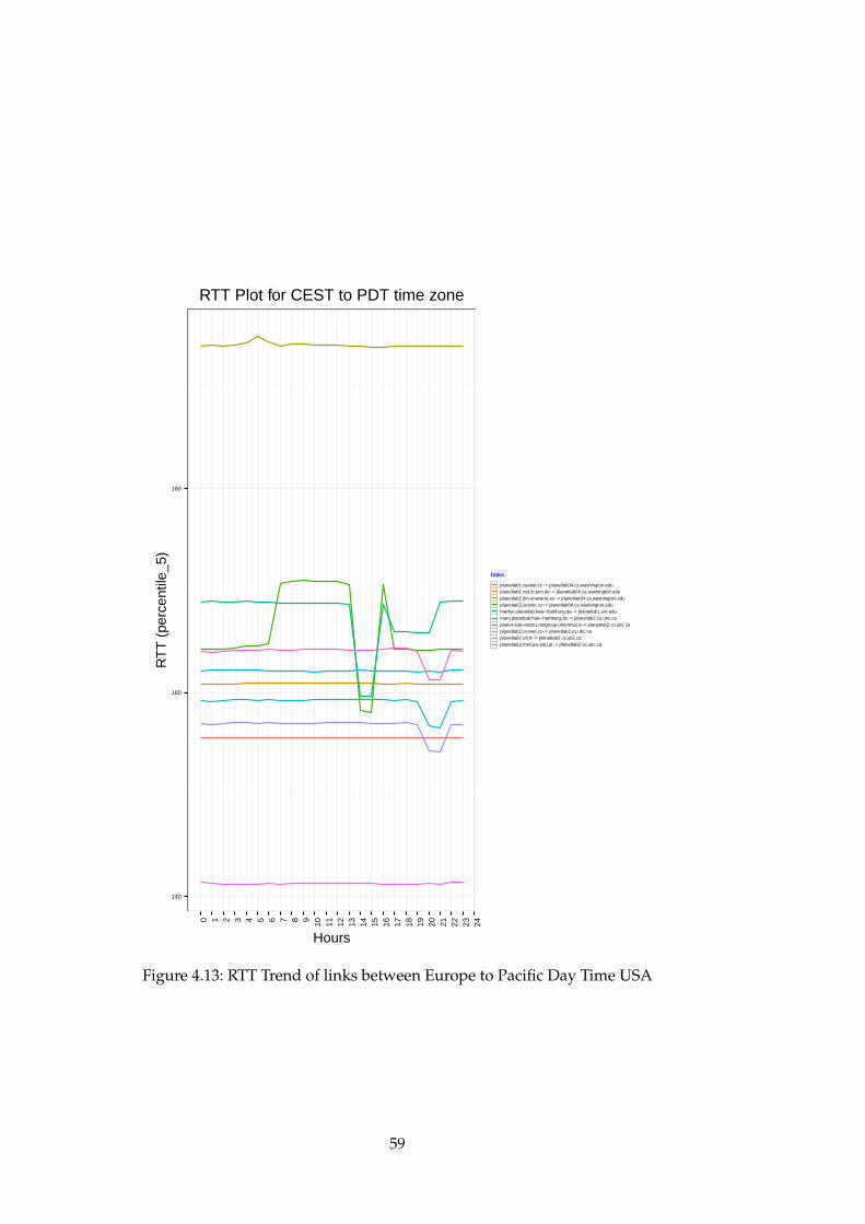
140

160

180

0 1 2 3 4 5 6 7 8 9 10 11 12 13 14 15 16 17 18 19 20 21 22 23 24

Hours

RT

T (

perc

entil

e_5)

links

planetlab1.cesnet.cz−> planetlab04.cs.washington.eduplanetlab1.net.in.tum.de−> planetlab04.cs.washington.eduplanetlab2.tlm.unavarra.es−> planetlab04.cs.washington.eduplanetlab3.cesnet.cz−> planetlab04.cs.washington.edumerkur.planetlab.haw−hamburg.de−> planetlab1.unr.edumars.planetlab.haw−hamburg.de−> planetlab2.cs.ubc.caplanet−lab−node1.netgroup.uniroma2.it−> planetlab2.cs.ubc.caplanetlab2.cesnet.cz−> planetlab2.cs.ubc.caplanetlab2.utt.fr−> planetlab2.cs.ubc.caplanetlab3.mini.pw.edu.pl−> planetlab2.cs.ubc.ca

RTT Plot for CEST to PDT time zone

Figure 4.13: RTT Trend of links between Europe to Pacific Day Time USA

59

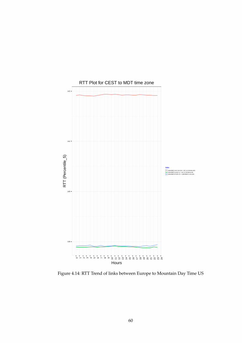
139

140

141

142

0 1 2 3 4 5 6 7 8 9 10 11 12 13 14 15 16 17 18 19 20 21 22 23 24

Hours

RT

T (

Per

cent

ile_5

)

links

planetlab1.net.in.tum.de−> pl1.cs.montana.eduplanetlab3.cesnet.cz−> pl1.cs.montana.eduplanetlab3.inf.ethz.ch−> planetlab2.cs.du.edu

RTT Plot for CEST to MDT time zone

Figure 4.14: RTT Trend of links between Europe to Mountain Day Time US

60

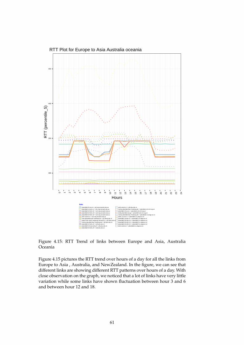
300

350

400

450

0 1 2 3 4 5 6 7 8 9 10 11 12 13 14 15 16 17 18 19 20 21 22 23 24

Hours

RT

T (

perc

entil

e_5)

links

planetlab1.ifi.uio.no−> pl1.eng.monash.edu.auplanetlab2.cesnet.cz−> pl1.eng.monash.edu.auplanetlab2.inf.ethz.ch−> pl1.eng.monash.edu.auplanetlab3.inf.ethz.ch−> pl1.eng.monash.edu.auplanetlab4.inf.ethz.ch−> pl1.eng.monash.edu.auple2.cesnet.cz−> pl1.eng.monash.edu.aumars.planetlab.haw−hamburg.de−> pl2.6test.edu.cnplanet−lab−node1.netgroup.uniroma2.it−> pl2.6test.edu.cnmerkur.planetlab.haw−hamburg.de−> pl2.pku.edu.cnplanetlab2.inf.ethz.ch−> pl2.pku.edu.cnplanetlab3.mini.pw.edu.pl−> pl2.pku.edu.cnplanetlab4.inf.ethz.ch−> pl2.pku.edu.cn

ple2.cesnet.cz−> pl2.pku.edu.cnmerkur.planetlab.haw−hamburg.de−> planetlab−js2.cert.org.cnplanetlab1.ifi.uio.no−> planetlab−js2.cert.org.cnstella.planetlab.ntua.gr−> planetlab−js2.cert.org.cnmerkur.planetlab.haw−hamburg.de−> planetlab2.cs.otago.ac.nzplab1.cs.msu.ru−> planetlab2.cs.otago.ac.nzplanetlab2.cesnet.cz−> planetlab2.cs.otago.ac.nzplanetlab2.inf.ethz.ch−> planetlab2.cs.otago.ac.nzplanetlab3.inf.ethz.ch−> planetlab2.cs.otago.ac.nzplanetlab4.inf.ethz.ch−> planetlab2.cs.otago.ac.nzple2.cesnet.cz−> planetlab2.cs.otago.ac.nz

RTT Plot for Europe to Asia Australia oceania

Figure 4.15: RTT Trend of links between Europe and Asia, AustraliaOceania

Figure 4.15 pictures the RTT trend over hours of a day for all the links fromEurope to Asia , Australia, and NewZealand. In the figure, we can see thatdifferent links are showing different RTT patterns over hours of a day. Withclose observation on the graph, we noticed that a lot of links have very littlevariation while some links have shown fluctuation between hour 3 and 6and between hour 12 and 18.

61

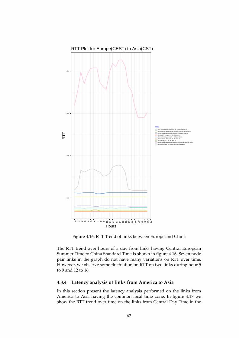
300

350

400

450

0 1 2 3 4 5 6 7 8 9 10 11 12 13 14 15 16 17 18 19 20 21 22 23 24

Hours

RT

T

links

mars.planetlab.haw−hamburg.de−> pl2.6test.edu.cnplanet−lab−node1.netgroup.uniroma2.it−> pl2.6test.edu.cnmerkur.planetlab.haw−hamburg.de−> pl2.pku.edu.cnplanetlab2.inf.ethz.ch−> pl2.pku.edu.cnplanetlab3.mini.pw.edu.pl−> pl2.pku.edu.cnplanetlab4.inf.ethz.ch−> pl2.pku.edu.cnple2.cesnet.cz−> pl2.pku.edu.cnmerkur.planetlab.haw−hamburg.de−> planetlab−js2.cert.org.cnplanetlab1.ifi.uio.no−> planetlab−js2.cert.org.cn

RTT Plot for Europe(CEST) to Asia(CST)

Figure 4.16: RTT Trend of links between Europe and China

The RTT trend over hours of a day from links having Central EuropeanSummer Time to China Standard Time is shown in figure 4.16. Seven nodepair links in the graph do not have many variations on RTT over time.However, we observe some fluctuation on RTT on two links during hour 5to 9 and 12 to 16.

4.3.4 Latency analysis of links from America to Asia

In this section present the latency analysis performed on the links fromAmerica to Asia having the common local time zone. In figure 4.17 weshow the RTT trend over time on the links from Central Day Time in the

62

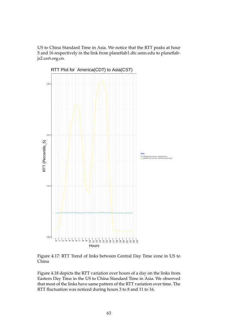
US to China Standard Time in Asia. We notice that the RTT peaks at hour5 and 16 respectively in the link from planetlab1.dtc.umn.edu to planetlab-js2.cert.org.cn.

200

210

220

230

0 1 2 3 4 5 6 7 8 9 10 11 12 13 14 15 16 17 18 19 20 21 22 23 24

Hours

RT

T (

Per

cent

ile_5

)

links

planetlab1.dtc.umn.edu−> pl2.pku.edu.cnplanetlab1.dtc.umn.edu−> planetlab−js2.cert.org.cn

RTT Plot for America(CDT) to Asia(CST)

Figure 4.17: RTT Trend of links between Central Day Time zone in US toChina

Figure 4.18 depicts the RTT variation over hours of a day on the links fromEastern Day Time in the US to China Standard Time in Asia. We observedthat most of the links have same pattern of the RTT variation over time. TheRTT fluctuation was noticed during hours 3 to 8 and 11 to 16.

63

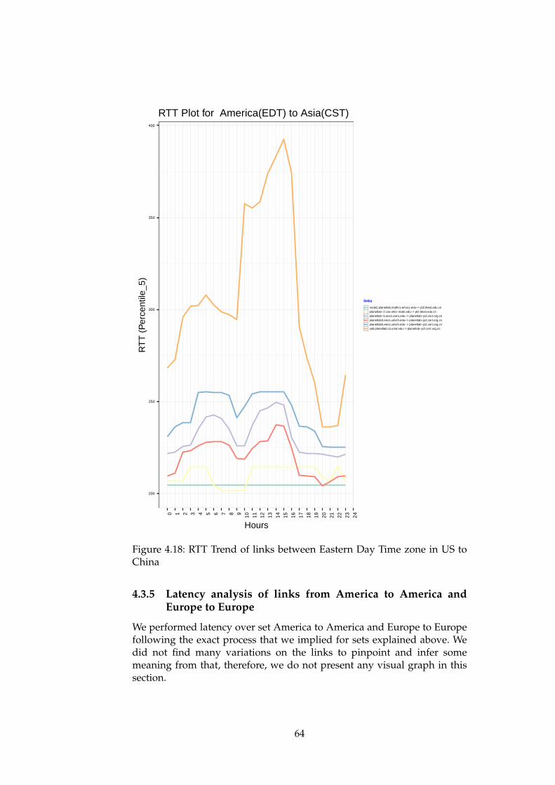
200

250

300

350

400

0 1 2 3 4 5 6 7 8 9 10 11 12 13 14 15 16 17 18 19 20 21 22 23 24

Hours

RT

T (

Per

cent

ile_5

)

links

node2.planetlab.mathcs.emory.edu−> pl2.6test.edu.cnplanetlab−2.cse.ohio−state.edu−> pl2.6test.edu.cnplanetlab−5.eecs.cwru.edu−> planetlab−js2.cert.org.cnplanetlab3.eecs.umich.edu−> planetlab−js2.cert.org.cnplanetlab5.eecs.umich.edu−> planetlab−js2.cert.org.cnsalt.planetlab.cs.umd.edu−> planetlab−js2.cert.org.cn

RTT Plot for America(EDT) to Asia(CST)

Figure 4.18: RTT Trend of links between Eastern Day Time zone in US toChina

4.3.5 Latency analysis of links from America to America andEurope to Europe

We performed latency over set America to America and Europe to Europefollowing the exact process that we implied for sets explained above. Wedid not find many variations on the links to pinpoint and infer somemeaning from that, therefore, we do not present any visual graph in thissection.

64

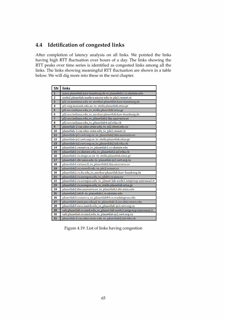
4.4 Idetification of congested links

After completion of latency analysis on all links. We pointed the linkshaving high RTT fluctuation over hours of a day. The links showing theRTT peaks over time series is identified as congested links among all thelinks. The links showing meaningful RTT fluctuation are shown in a tablebelow. We will dig more into these in the next chapter.

Figure 4.19: List of links having congestion

65

66

Chapter 5

Traceroute Analysis

In the previous chapter, we identified the links which have problemsamong all links. Based on those results, we move in the direction to identifythe links in the path between two ends of those links which are contributingto the congestion. For the sake of identification of the all the links inbetween source and destination and troubleshooting, them, Traceroute isa handy tool. Hence we move forward to analyzing the traceroute outputof respective links. In fact, we have run traceroute from one end of the linkto another end every 10 seconds for 3 weeks. . The detail analysis processand result are discussed in the sections below as following.

5.1 Parsing and retrieving data in designated for-mat

While running traceroute from source to destination, we have sent 10packets from source to destination therefore at each hop we have 10 RTTvalues ,among them, we picked up minimum value and corresponding IPaddress. At the same time, we subtract the RTT values of that hop withthe previous hop’s RTT value in order to calculate the hop delay. Thisprocess continues until the end of the file. Eventually, we got the file withinformation about each hop number along with corresponding RTT, IPaddress, and delay to reach to that hop from the previous hop.

5.2 Generating Time series data for each hop fromsource to destination

We have recorded every instance of traceroute along with Unix timestampso we can easily convert that Unix timestamp to hours . Thereafter, we cre-ate a bin with a size of an hour thus we have 24 bins for generating timeseries data. We put the data into their corresponding bins. More precisely,we binned RTT and hop to hop delay for all the hops. To finalize time seriesdata creation , we compute some statics like mean, median, and percentileto reduce the number of observation. In this way, we obtained one datapoint per each hour so that we can visualize the value over the time series

67

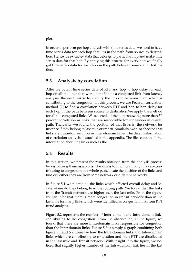
plot.

In order to perform per hop analysis with time series data, we need to havetime series data for each hop that lies in the path from source to destina-tion. Hence we extracted data that belongs to particular hop and make timeseries data for that hop. By applying this process for every hop we finallygot time series data for each hop in the path between source and destina-tion.

5.3 Analysis by correlation

After we obtain time series data of RTT and hop to hop delay for eachhop on all the links that were identified as a congested link from latencyanalysis, the next task is to identify the links in between them which iscontributing to the congestion. In this process, we use Pearson correlationmethod [2] to find a correlation between RTT and hop to hop delay foreach hop in the path between source to destination.We apply the methodfor all the congested links. We selected all the hops showing more than 50percent correlation as links that are responsible for congestion in overallpath. Thereafter we found the position of that links in the network forinstance if they belong to last mile or transit. Similarly, we also checked thatlinks are intra-domain links or Inter-domain links. The detail informationof correlation analysis is attached in the appendix. The files contain all theinformation about the links such as the

5.4 Results

In this section, we present the results obtained from the analysis processby visualizing them as graphs. The aim is to find how many links are con-tributing to congestion in a whole path, locate the position of the links andfind out either they are from same network or different networks.

In figure 5.1 we plotted all the links which affected overall delay and lo-cate where do they belong to in the routing path. We found that the linksfrom the Transit network are higher than the last mile. From the figure,we can infer that there is more congestion in transit network than in thelast mile for many links which were identified as congestion link from RTTtrend analysis.

Figure 5.2 represents the number of Inter-domain and Intra-domain linkscontributing to the congestion. From the observation, at the figure, wefound that there are more Intra-domain links responsible for congestionthan the Inter-domain links. Figure 5.3 is simply a graph combining bothfigure 5.1 and 5.2. Here we how the Intra-domain links and Inter-domainlinks which are contributing to congestion and high RTT are distributedin the last mile and Transit network. With insight into the figure, we no-ticed that slightly higher number of the Intra-domain link lies in the last

68

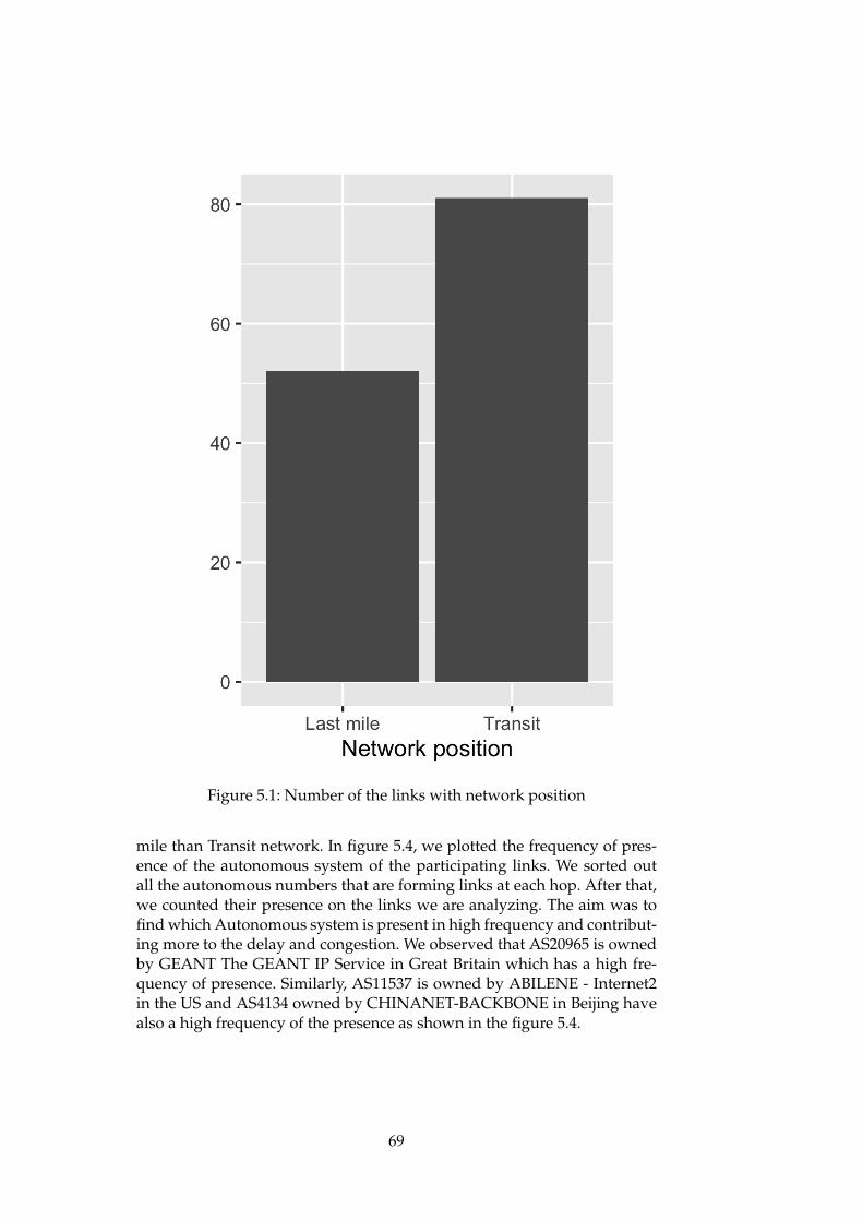
Figure 5.1: Number of the links with network position

mile than Transit network. In figure 5.4, we plotted the frequency of pres-ence of the autonomous system of the participating links. We sorted outall the autonomous numbers that are forming links at each hop. After that,we counted their presence on the links we are analyzing. The aim was tofind which Autonomous system is present in high frequency and contribut-ing more to the delay and congestion. We observed that AS20965 is ownedby GEANT The GEANT IP Service in Great Britain which has a high fre-quency of presence. Similarly, AS11537 is owned by ABILENE - Internet2in the US and AS4134 owned by CHINANET-BACKBONE in Beijing havealso a high frequency of the presence as shown in the figure 5.4.

69

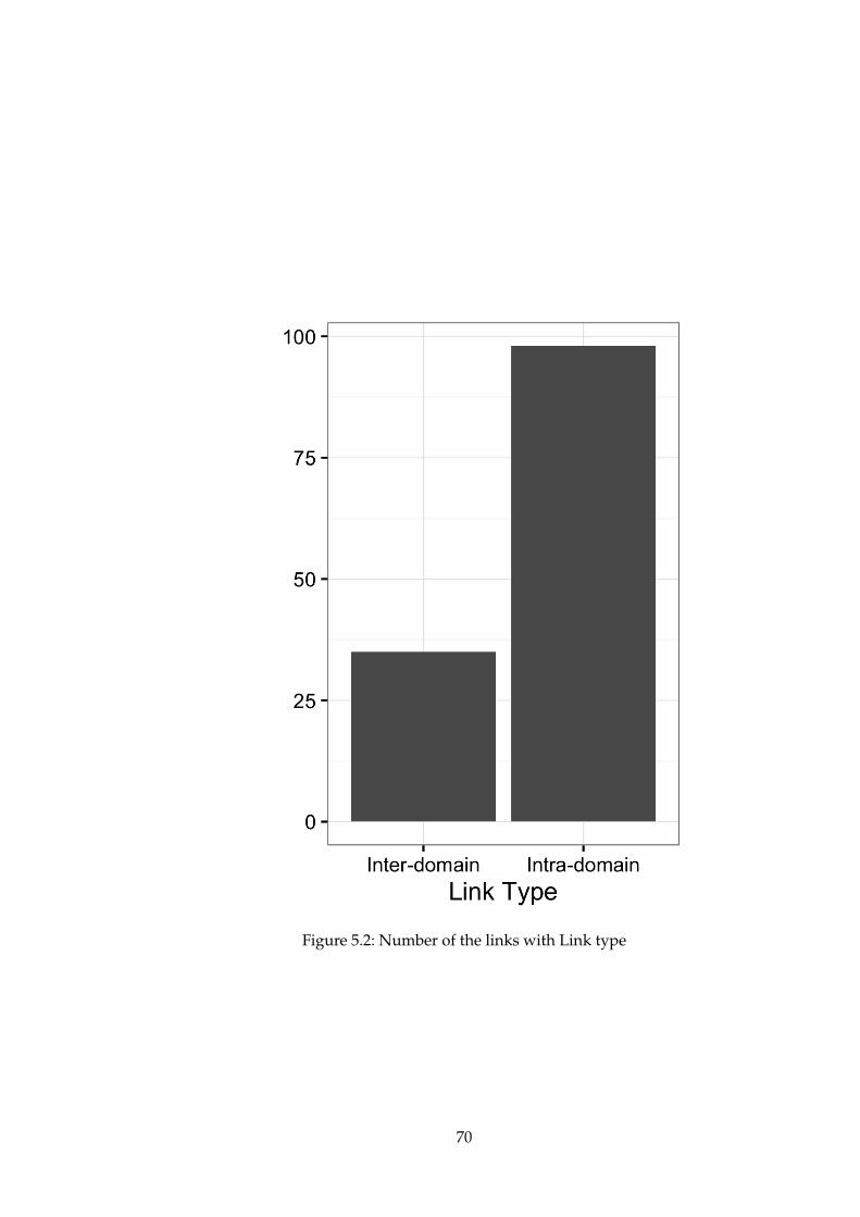
Figure 5.2: Number of the links with Link type

70

Figure 5.3: Number of the links with network position and link type

71

Figure 5.4: Number of the links with network position and link type

72

Chapter 6

Discussion and Conclusion

6.1 Discussion on results from latency analysis

In this section we present some highlights of result from latency analysis.we analyzed around 200 node pair links investigating the latency trendovertime. As a result, we found 31 node pair links showing peak RTT valuesover the time. From a close observation of results from latency analysis, wefound 4 patterns by gathering the links with similar patterns together. Thelatency trend among those node pair links as shown in figure 6.2 below.Figure 6.1 depicts conversion of GMT to respective local time where theshaded area represents the business hours of respective time zones.

GMT   EDT  US  

PDT  US  

MDT  US  

CDT  US  

CST  China  

CEST  Europe  

EEST  Europe  

0   8  PM   5  PM   6  PM   7  PM   8  AM   2  AM   3  AM  1   9  PM   6  PM   7  PM   8  PM   9  AM   3  AM   4  AM  2   10  PM   7  PM   8  PM   9  PM   10  AM   4  AM   5  AM  3   11  PM   8  PM   9  PM   10  PM   11  AM   5  AM   6  AM  4   12  AM   9  PM   10  PM   11  PM   12  PM   6  AM   7  AM  5   1  AM   10  PM   11  PM   12  AM   1  PM   7  AM   8  AM  6   2  AM   11  PM   12  AM   1  AM   2  PM   8  AM   9  AM  7   3  AM   12  AM   1  AM   2  AM   3  PM   9  AM   10  AM  8   4  AM   1  AM   2  AM   3  AM   4  PM   10  AM   11  AM  9   5  AM   2  AM   3  AM   4  AM   5  PM   11  AM   12  PM  10   6  AM   3  AM   4  AM   5  AM   6  PM   12  PM   1  PM  11   7  AM   4  AM   5  AM   6  AM   7  PM   1  PM   2  PM  12   8  AM   5  AM   6  AM   7  AM   8  PM   2  PM   3  PM  13   9  AM   6  AM   7  AM   8  AM   9  PM   3  PM   4  PM  14   10  AM   7  AM   8  AM   9  AM   10  PM   4  PM   5  PM  15   11  AM   8  AM   9  AM   10  AM   11  PM   5  PM   6  PM  16   12  PM   9  AM   10  AM   11  AM   12  AM   6  PM   7  PM  17   1  PM   10  AM   11  AM   12  PM   1  AM   7  PM   8  PM  18   2  PM   11  AM   12  PM   1  PM   2  AM   8  PM   9  PM  19   3  PM   12  PM   1  PM   2  PM   3  AM   9  PM   10  PM  20   4  PM   1  PM   2  PM   3  PM   4  AM   10  PM   11  PM  21   5  PM   2  PM   3  PM   4  PM   5  AM   11  PM   12  AM  22   6  PM   3  PM   4  PM   5  PM   6  AM   12  AM   1  AM  23   7  PM   4  PM   5  PM   6  PM   7  AM   1  AM   2  AM      

Figure 6.1: GMT to Local time chart

73

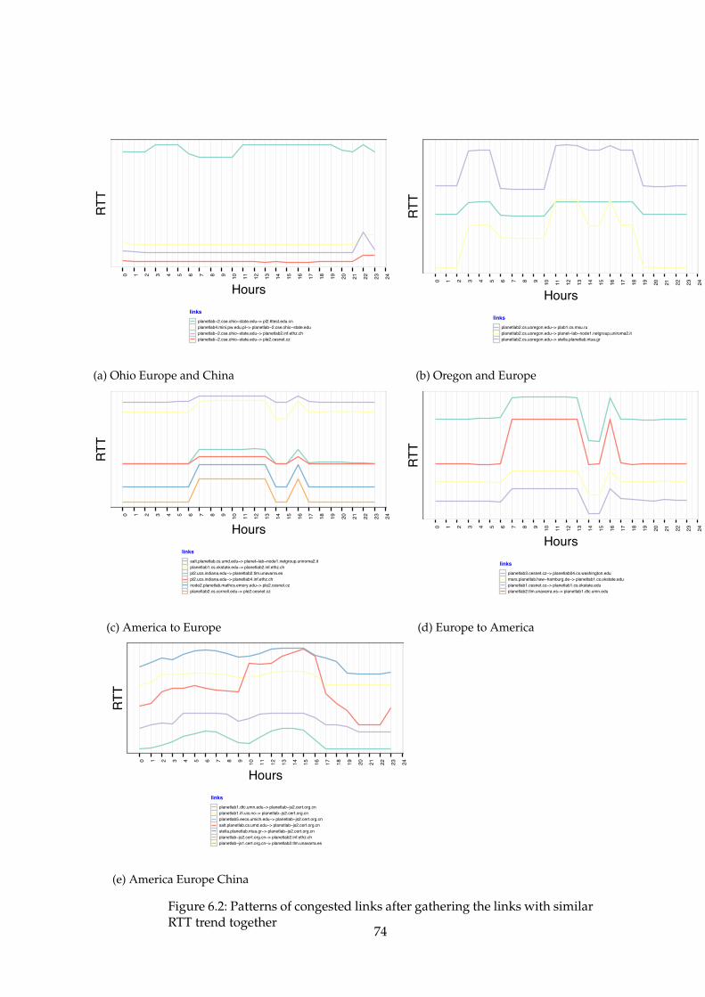
0 1 2 3 4 5 6 7 8 9 10 11 12 13 14 15 16 17 18 19 20 21 22 23 24

Hours

RTT

linksplanetlab−2.cse.ohio−state.edu−> pl2.6test.edu.cnplanetlab4.mini.pw.edu.pl−> planetlab−2.cse.ohio−state.eduplanetlab−2.cse.ohio−state.edu−> planetlab2.inf.ethz.chplanetlab−2.cse.ohio−state.edu−> ple2.cesnet.cz

(a) Ohio Europe and China

0 1 2 3 4 5 6 7 8 9 10 11 12 13 14 15 16 17 18 19 20 21 22 23 24

Hours

RTT

linksplanetlab2.cs.uoregon.edu−> plab1.cs.msu.ruplanetlab2.cs.uoregon.edu−> planet−lab−node1.netgroup.uniroma2.itplanetlab2.cs.uoregon.edu−> stella.planetlab.ntua.gr

(b) Oregon and Europe

0 1 2 3 4 5 6 7 8 9 10 11 12 13 14 15 16 17 18 19 20 21 22 23 24

Hours

RTT

linkssalt.planetlab.cs.umd.edu−> planet−lab−node1.netgroup.uniroma2.itplanetlab1.cs.okstate.edu−> planetlab2.inf.ethz.chpl2.ucs.indiana.edu−> planetlab2.tlm.unavarra.espl2.ucs.indiana.edu−> planetlab4.inf.ethz.chnode2.planetlab.mathcs.emory.edu−> ple2.cesnet.czplanetlab2.cs.cornell.edu−> ple2.cesnet.cz

(c) America to Europe

0 1 2 3 4 5 6 7 8 9 10 11 12 13 14 15 16 17 18 19 20 21 22 23 24

Hours

RTT

linksplanetlab3.cesnet.cz−> planetlab04.cs.washington.edumars.planetlab.haw−hamburg.de−> planetlab1.cs.okstate.eduplanetlab1.cesnet.cz−> planetlab1.cs.okstate.eduplanetlab2.tlm.unavarra.es−> planetlab1.dtc.umn.edu

(d) Europe to America

0 1 2 3 4 5 6 7 8 9 10 11 12 13 14 15 16 17 18 19 20 21 22 23 24

Hours

RTT

linksplanetlab1.dtc.umn.edu−> planetlab−js2.cert.org.cnplanetlab1.ifi.uio.no−> planetlab−js2.cert.org.cnplanetlab5.eecs.umich.edu−> planetlab−js2.cert.org.cnsalt.planetlab.cs.umd.edu−> planetlab−js2.cert.org.cnstella.planetlab.ntua.gr−> planetlab−js2.cert.org.cnplanetlab−js2.cert.org.cn−> planetlab2.inf.ethz.chplanetlab−js1.cert.org.cn−> planetlab2.tlm.unavarra.es

(e) America Europe China

Figure 6.2: Patterns of congested links after gathering the links with similarRTT trend together

74

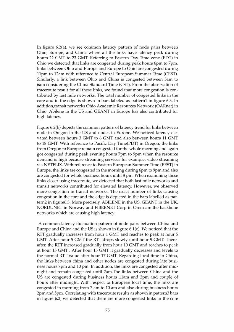
In figure 6.2(a), we see common latency pattern of node pairs betweenOhio, Europe, and China where all the links have latency peak duringhours 22 GMT to 23 GMT. Referring to Eastern Day Time zone (EDT) inOhio we detected that links are congested during peak hours 6pm to 7pm.links between Ohio and Europe and Europe to Ohio are congested during11pm to 12am with reference to Central European Summer Time (CEST).Similarly, a link between Ohio and China is congested between 5am to6am considering the China Standard Time (CST). From the observation oftraceroute result for all these links, we found that more congestion is con-tributed by last mile networks. The total number of congested links in thecore and in the edge is shown in bars labeled as pattern1 in figure 6.3. Inaddition,transit networks Ohio Academic Resources Network (OARnet) inOhio, Abilene in the US and GEANT in Europe has also contributed forhigh latency.

Figure 6.2(b) depicts the common pattern of latency trend for links betweennode in Oregon in the US and nodes in Europe. We noticed latency ele-vated between hours 3 GMT to 6 GMT and also between hours 11 GMTto 18 GMT. With reference to Pacific Day Time(PDT) in Oregon, the linksfrom Oregon to Europe remain congested for the whole morning and againgot congested during peak evening hours 7pm to 9pm when the resourcedemand is high because streaming services for example, video streamingvia NETFLIX. With reference to Eastern European Summer Time (EEST) inEurope, the links are congested in the morning during 6pm to 9pm and alsoare congested for whole business hours until 8 pm. When examining theselinks closer using traceroute, we detected that both last mile networks andtransit networks contributed for elevated latency. However, we observedmore congestion in transit networks. The exact number of links causingcongestion in the core and the edge is depicted in the bars labelled as pat-tern2 in figure6.3. More precisely, ABILENE in the US, GEANT in the UK,NORDUNET in Norway and FIBERNET Corp in Orem are the backbonenetworks which are causing high latency.

A common latency fluctuation pattern of node pairs between China andEurope and China and the US is shown in figure 6.1(e). We noticed that theRTT gradually increases from hour 1 GMT and reaches to peak at hour 5GMT. After hour 5 GMT the RTT drops slowly until hour 9 GMT. There-after, the RTT increased gradually from hour 10 GMT and reaches to peakat hour 15 GMT . After hour 15 GMT it gradually decreases and levels tothe normal RTT value after hour 17 GMT. Regarding local time in China,the links between china and other nodes are congested during late busi-ness hours 7pm and 10 pm. In addition, the links are congested after mid-night and remain congested until 2am.The links between China and theUS are congested during business hours 11am and 2pm and couple ofhours after midnight. With respect to European local time, the links arecongested in morning from 7 am to 10 am and also during business hours2pm and 5pm. Correlating with traceroute results as shown in pattern3 barsin figure 6.3, we detected that there are more congested links in the core

75

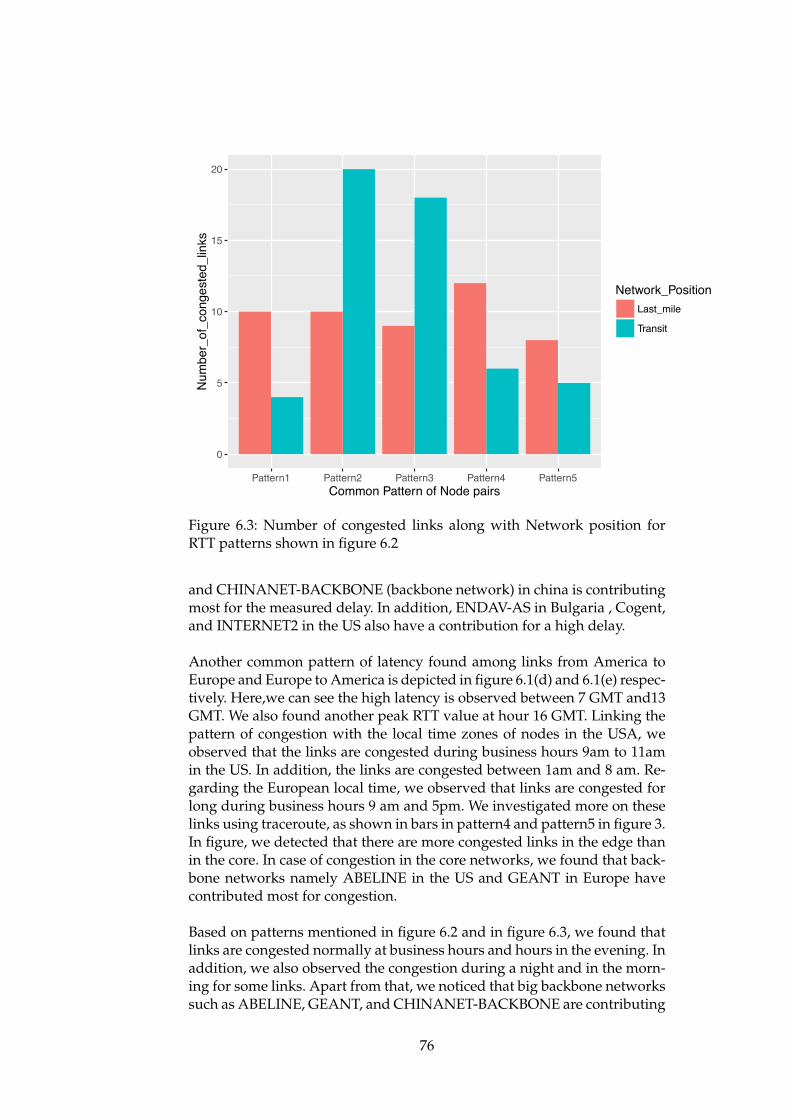
0

5

10

15

20

Pattern1 Pattern2 Pattern3 Pattern4 Pattern5Common Pattern of Node pairs

Num

ber_

of_c

onge

sted

_lin

ks

Network_PositionLast_mile

Transit

Figure 6.3: Number of congested links along with Network position forRTT patterns shown in figure 6.2

and CHINANET-BACKBONE (backbone network) in china is contributingmost for the measured delay. In addition, ENDAV-AS in Bulgaria , Cogent,and INTERNET2 in the US also have a contribution for a high delay.

Another common pattern of latency found among links from America toEurope and Europe to America is depicted in figure 6.1(d) and 6.1(e) respec-tively. Here,we can see the high latency is observed between 7 GMT and13GMT. We also found another peak RTT value at hour 16 GMT. Linking thepattern of congestion with the local time zones of nodes in the USA, weobserved that the links are congested during business hours 9am to 11amin the US. In addition, the links are congested between 1am and 8 am. Re-garding the European local time, we observed that links are congested forlong during business hours 9 am and 5pm. We investigated more on theselinks using traceroute, as shown in bars in pattern4 and pattern5 in figure 3.In figure, we detected that there are more congested links in the edge thanin the core. In case of congestion in the core networks, we found that back-bone networks namely ABELINE in the US and GEANT in Europe havecontributed most for congestion.

Based on patterns mentioned in figure 6.2 and in figure 6.3, we found thatlinks are congested normally at business hours and hours in the evening. Inaddition, we also observed the congestion during a night and in the morn-ing for some links. Apart from that, we noticed that big backbone networkssuch as ABELINE, GEANT, and CHINANET-BACKBONE are contributing

76

more to the congestion in the core networks (a detailed analysis on thesebackbone networks are presented in the next section). However, the edgenetworks are also causing the congestion.The exact comparison of conges-tion in the core networks and the edge networks including all congestednode pairs is presented in next section of discussion.

From insight into the latency analysis results, we observed that only nodepairs links having end nodes from the different continent are congested.This means that links with very long path crossing global continents arecongested. In figure 6.2, we can see that all congested node pair links hav-ing end nodes from different continents. In figure 6.4 , the latency trend oflinks having end nodes only in America is depicted. Similarly, figure 6.5shows the RTT trend of the links where end nodes belong to Europe only.In the both figures, we did not notice significant RTT variation.

50

100

150

0 1 2 3 4 5 6 7 8 9 10 11 12 13 14 15 16 17 18 19 20 21 22 23Hours

RT

T

links

planetlab1.cs.okstate.edu−> pl1.cs.montana.eduplanetlab2.cs.uoregon.edu−> planetlab−2.cse.ohio−state.eduplanetlab1.cs.du.edu−> planetlab1.cs.okstate.eduplanetlab2.cs.cornell.edu−> planetlab1.cs.okstate.eduplanetlab5.eecs.umich.edu−> planetlab1.cs.okstate.edusalt.planetlab.cs.umd.edu−> planetlab1.cs.okstate.eduplanetlab1.pop−mg.rnp.br−> planetlab1.dtc.umn.eduplanetlab1.unr.edu−> planetlab1.dtc.umn.edunode2.planetlab.mathcs.emory.edu−> planetlab2.cs.ubc.caplanetlab−2.cse.ohio−state.edu−> planetlab2.cs.ubc.caplanetlab−5.eecs.cwru.edu−> planetlab2.cs.ubc.caplanetlab2.cs.cornell.edu−> planetlab2.cs.ubc.caplanetlab1.unr.edu−> planetlab2.pop−mg.rnp.br

Figure 6.4: RTT trend America to America

77

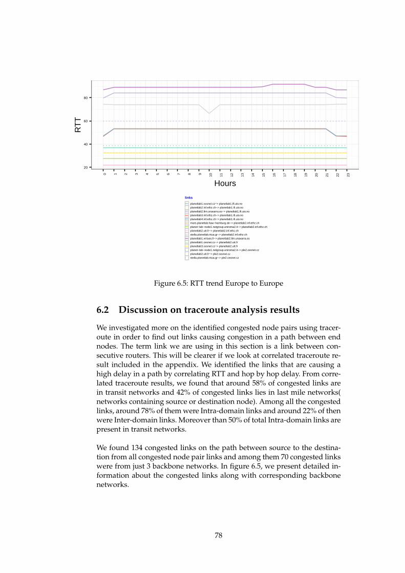
20

40

60

80

0 1 2 3 4 5 6 7 8 9 10 11 12 13 14 15 16 17 18 19 20 21 22 23

Hours

RT

T

links

planetlab1.cesnet.cz−> planetlab1.ifi.uio.noplanetlab2.inf.ethz.ch−> planetlab1.ifi.uio.noplanetlab2.tlm.unavarra.es−> planetlab1.ifi.uio.noplanetlab3.inf.ethz.ch−> planetlab1.ifi.uio.noplanetlab4.inf.ethz.ch−> planetlab1.ifi.uio.nomars.planetlab.haw−hamburg.de−> planetlab2.inf.ethz.chplanet−lab−node1.netgroup.uniroma2.it−> planetlab2.inf.ethz.chplanetlab2.utt.fr−> planetlab2.inf.ethz.chstella.planetlab.ntua.gr−> planetlab2.inf.ethz.chplanetlab1.virtues.fi−> planetlab2.tlm.unavarra.esplanetlab1.cesnet.cz−> planetlab2.utt.frplanetlab3.cesnet.cz−> planetlab2.utt.frplanet−lab−node1.netgroup.uniroma2.it−> ple2.cesnet.czplanetlab2.utt.fr−> ple2.cesnet.czstella.planetlab.ntua.gr−> ple2.cesnet.cz

Figure 6.5: RTT trend Europe to Europe

6.2 Discussion on traceroute analysis results

We investigated more on the identified congested node pairs using tracer-oute in order to find out links causing congestion in a path between endnodes. The term link we are using in this section is a link between con-secutive routers. This will be clearer if we look at correlated traceroute re-sult included in the appendix. We identified the links that are causing ahigh delay in a path by correlating RTT and hop by hop delay. From corre-lated traceroute results, we found that around 58% of congested links arein transit networks and 42% of congested links lies in last mile networks(networks containing source or destination node). Among all the congestedlinks, around 78% of them were Intra-domain links and around 22% of thenwere Inter-domain links. Moreover than 50% of total Intra-domain links arepresent in transit networks.

We found 134 congested links on the path between source to the destina-tion from all congested node pair links and among them 70 congested linkswere from just 3 backbone networks. In figure 6.5, we present detailed in-formation about the congested links along with corresponding backbonenetworks.

78

Figure 6.6: Number of the links with network position and link type forGEANT, ABILENE and CHINANET-BACKBONE backbone networks

We noticed that packets in all links from America to Europe need transitfrom AS11537 when leaving America and need transit from AS20965 whenentering Europe and vice versa. Whereas AS4134 provides transit forpackets entering or leaving china and also provides connection service forregional networks. From the information in figure 6, we can see that almost50% of the congested links lies within these ASes.

6.3 Limitations

We have conducted experiments in PlanetLab testbed and it has somelimitations. All the nodes in PlanetLab are at universities or research centersand they are likely to use educational networks such as ABILENE andGEANT therefore what we see here is limited to PlanetLab only but theInternet is very broad in a scope. Therefore, we fail to measure real accessnetworks as experienced by regular users. PlanetLab nodes are used by alarge number of researchers and students sharing limited resources henceit can also be congested. Hence, our finding might have been affected bycongestion in the PlanentLab. Apart from this, the measurement is limitedto RTT measurement between node pairs of the PlanetLab nodes. Wehave not performed loss analysis correlating RTT analysis hence the RTTanalysis might not be precise. Moreover, we are using Traceroute whichinfers latency and gives a nice overview of network hops but it is notprecise. As traceroute gives latency value on the basis of the only forwardpath, the latency value is not precise if there is congestion in reverse path.Furthermore, traceroute might not insight properly where is congestionwhen there are multiple routing policies and asymmetric routes in thenetwork.

6.4 Conclusion

Networking is growing rapidly in terms of size and complexity challengingthe performance of the network. In order to cope this, we have invested alot of money to increase capacity, speed and upgrade technologies. How-ever, the performance of the network is not satisfactory as the underlyingproblem is congested links which are the bottleneck for the network per-formance. In addition, we are mostly focused on only improving the per-

79

formance of the edge networks. However, the performance of the networkis degraded in the core networks nowadays [30, 41]. Hence, in this thesis,we devised experiments in the PlanetLab testbed to examine congestion inthe edge networks as well as in the core networks. We measured end to enddelay of more than 200 node pairs where nodes are distributed all over theworld and detected the congested node pairs among them. Using tracer-oute analysis on the congested node pairs, we found the congested linksbetween node pairs and located them in the network. Hence, we detectedaround 42% congestion in the edge networks whereas around 58% conges-tion in the core networks. Moreover, we observed that intra-domain linkscontributed more for congestion than inter-domain links.

6.5 Future works

Although we calculated packet loss, we did not have time to analyze theloss statistics that were gathered. Therefore, we can correlate the result fromtraceroute analysis with loss statistics and make the result more precise. Weare limited to only a few nodes in the PlanetLab so that we can increasethe number of nodes in the future and make the experiment complete andmore meaningful. Similarly, we can increase the duration of experimentsignificantly for instance more than 6 weeks so that we might see moreappropriate variation on latency. Another improvement can be made byadding people's home networks for the experiments. In this thesis, we arelimited only to educational and research networks in the PlanetLab. If weadd home networks we can broaden the scope as commercial ISP networkswill be added up for analysis.

80

Bibliography

[1] National Media Museum Bradford BD1 1NQ. “A Brief History of theInternet.” In: (2011).

[2] Alan Agresti and Barbara F Agresti. “Statistical Methods for the.” In:Social Sciences. CA: Dellen Publishers (1970).

[3] A de A Antonio et al. “Revisitando Metrologia de Redes: DoPassadoas Novas Tendências.” In: ().

[4] Jose M. Barcelo, Juan I. Nieto-Hipolito, and Jorge Garcıa-Vidal.“Study of Internet autonomous system interconnectivity from BGProuting tables.” In: (2004).

[5] Steven Bauer, David D Clark, and William Lehr. “The evolution ofinternet congestion.” In: TPRC. 2009.

[6] Jean-Chrysotome Bolot. “End-to-end packet delay and loss behav-ior in the Internet.” In: ACM SIGCOMM Computer Communication Re-view. Vol. 23. 4. ACM. 1993, pp. 289–298.

[7] Michael S Borella et al. “Internet packet loss: Measurement andimplications for end-to-end QoS.” In: Architectural and OS Supportfor Multimedia Applications/Flexible Communication Systems/WirelessNetworks and Mobile Computing., 1998 Proceedings of the 1998 ICPPWorkshops on. IEEE. 1998, pp. 3–12.

[8] CJ Bovy et al. “Analysis of end-to-end delay measurements inInternet.” In: Proceedings of ACM Conference on Passive and ActiveLeasurements (PAM), Fort Collins, Colorado, USA. 2002.

[9] Robert L Carter and Mark E Crovella. “Measuring bottleneck linkspeed in packet-switched networks.” In: Performance evaluation 27(1996), pp. 297–318.

[10] Marshini Chetty et al. “Why is my internet slow?: making networkspeeds visible.” In: Proceedings of the SIGCHI Conference on HumanFactors in Computing Systems. ACM. 2011, pp. 1889–1898.

[11] Chiara Chirichella and Davide Rossi. “To the Moon and back: areInternet bufferbloat delays really that large?” In: Computer Commu-nications Workshops (INFOCOM WKSHPS), 2013 IEEE Conference on.IEEE. 2013, pp. 417–422.

[12] Brent Chun et al. “Planetlab: an overlay testbed for broad-coverageservices.” In: ACM SIGCOMM Computer Communication Review 33.3(2003), pp. 3–12.

81

[13] Cisco. “Border Gateway Protocol.” In: Internetworking TechnologiesHandbook. Cisco Press, Sept. 2003. Chap. 41, pp. 663–673.

[14] David D Clark et al. “Measurement and Analysis of InternetInterconnection and Congestion.” In: 2014 TPRC Conference Paper.2014.

[15] Douglas E. Comer. The Internet Book: Everything You Need to Knowabout Computer Networking and How the Internet Works. 4th ed. PrenticeHall, 2006. ISBN: 0132335530.

[16] Constantine Dovrolis. “The Evolution and Economics of InternetInterconnections.” In: ().

[17] Aiguo Fei et al. “Measurements on delay and hop-count of theInternet.” In: IEEE GLOBECOM. Vol. 98. 1998.

[18] Lixin Gao. “On inferring autonomous system relationships in theInternet.” In: IEEE/ACM Transactions on Networking (ToN) 9.6 (2001),pp. 733–745.

[19] Daniel Genin and Jolene Splett. “Where in the Internet is conges-tion?” In: arXiv preprint arXiv:1307.3696 (2013).

[20] Jim Gettys and Kathleen Nichols. “Bufferbloat: dark buffers in theinternet.” In: Communications of the ACM 55.1 (2012), pp. 57–65.

[21] Ningning Hu et al. “A measurement study of internet bottlenecks.”In: INFOCOM 2005. 24th Annual Joint Conference of the IEEE Computerand Communications Societies. Proceedings IEEE. Vol. 3. IEEE. 2005,pp. 1689–1700.

[22] Ningning Hu et al. Locating Internet bottlenecks: Algorithms, measure-ments, and implications. Vol. 34. 4. ACM, 2004.

[23] Gianluca Iannaccone, Martin May, and Christophe Diot. “Aggregatetraffic performance with active queue management and drop fromtail.” In: ACM SIGCOMM Computer Communication Review 31.3(2001), pp. 4–13.

[24] Olumuyiwa Ibidunmoye. “Performance Problem Diagnosis in CloudInfrastructures.” In: (2016).

[25] Olumuyiwa Ibidunmoye, Francisco Hernández-Rodriguez, and ErikElmroth. “Performance anomaly detection and bottleneck identifica-tion.” In: ACM Computing Surveys (CSUR) 48.1 (2015), p. 4.

[26] Cisco Visual Networking Index. “Global Mobile Data Traffic Fore-cast Update 2014–2019. White Paper c11-520862.” In: Available onhttp://www. cisco. com/c/en/us/solutions/collateral/service-provider/visual-networking-indexvni/white_paper_c11-520862. html ().

[27] Cisco Visual Networking Index. Global Mobile Data Traffic ForecastUpdate 2015–2020 White Paper.

[28] Ivan Kaminow and Tingye Li. Optical Fiber Telecommunications IV-B:Systems and Impairments. Academic Press, 2002. ISBN: 0-12-395172-0.

82

[29] Dan Komosny et al. “PlanetLab Europe as Geographically-DistributedTestbed for Software Development and Evaluation.” In: Advances inElectrical and Electronic Engineering 13.2 (2015), pp. 137–146.

[30] Tom Leighton. “Improving performance on the internet.” In: Commu-nications of the ACM 52.2 (2009), pp. 44–51.

[31] Chuan Lin et al. “Research on bottleneck-delay in internet basedon IP united mapping.” In: Peer-to-Peer Networking and Applications(2016), pp. 1–13.

[32] Matthew Luckie et al. “Challenges in Inferring Internet InterdomainCongestion.” In: Proceedings of the 2014 Conference on Internet Measure-ment Conference. ACM. 2014, pp. 15–22.

[33] Ivan Marsic. Computer Networks: Performance and Quality of Service.Ivan Marsic, 2010. ISBN: N/A.

[34] Ingrid Melve et al. “A study on network performance metrics andtheir composition.” In: Campus-Wide Information Systems 23.4 (2006),pp. 268–282.

[35] Erik Nygren, Ramesh K Sitaraman, and Jennifer Sun. “The Akamainetwork: a platform for high-performance internet applications.” In:ACM SIGOPS Operating Systems Review 44.3 (2010), pp. 2–19.

[36] Bruno Quoitin et al. “Interdomain traffic engineering with BGP.” In:Communications Magazine, IEEE 41.5 (2003), pp. 122–128.

[37] Lawrence G Roberts. “Beyond Moore’s law: Internet growth trends.”In: Computer 33.1 (2000), pp. 117–119.

[38] Seungwan Ryu, Christopher Rump, and Chunming Qiao. “Advancesin active queue management (AQM) based TCP congestion control.”In: Telecommunication Systems 25.3-4 (2004), pp. 317–351.

[39] Halabi Sam. Internet routing architectures. Pearson Education India,2008.

[40] Ankit Singla et al. “The internet at the speed of light.” In: Proceedingsof the 13th ACM Workshop on Hot Topics in Networks. ACM. 2014, p. 1.

[41] Ramesh K Sitaraman. “Network performance: Does it really matterto users and by how much?” In: 2013 Fifth International Conferenceon Communication Systems and Networks (COMSNETS). IEEE. 2013,pp. 1–10.

[42] Internet Society. Global Internet Report 2014 Internet Society. Tech. rep.Internet Society, May 2014.

[43] Michael Welzl. Network congestion control: managing internet traffic.John Wiley & Sons, 2005.

[44] Mark Winther. Tier 1 ISP s : What They Are and Why They Are Important.WHITE PAPER. Global Headquarters: 5 Speen Street Framingham,MA 01701 USA: IDC, May 2006.

83

[45] Yang Richard Yang and Simon S Lam. “General AIMD congestioncontrol.” In: Network Protocols, 2000. Proceedings. 2000 InternationalConference on. IEEE. 2000, pp. 187–198.

84

Appendices

85

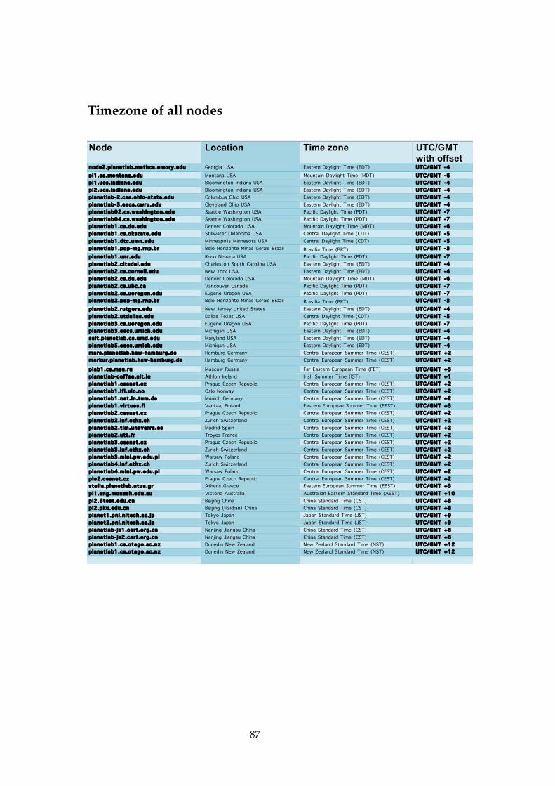
Timezone of all nodes

Node Location Time zone UTC/GMT with offset

node2.p lanet lab .mathcs .emory .edu Georgia USA Eastern Daylight Time (EDT) UTC/GMT -4 p l1 .cs .montana.edu Montana USA Mountain Daylight Time (MDT) UTC/GMT -6 p l1 .ucs . ind iana .edu Bloomington Indiana USA Eastern Daylight Time (EDT) UTC/GMT -4 p l2 .ucs . ind iana .edu Bloomington Indiana USA Eastern Daylight Time (EDT) UTC/GMT -4 p lanet lab-2 .cse .oh io-state .edu Columbus Ohio USA Eastern Daylight Time (EDT) UTC/GMT -4 p lanet lab-5 .eecs .cwru .edu Cleveland Ohio USA Eastern Daylight Time (EDT) UTC/GMT -4 p lanet lab02.cs .wash ington.edu Seattle Washington USA Pacific Daylight Time (PDT) UTC/GMT -7 p lanet lab04.cs .wash ington.edu Seattle Washington USA Pacific Daylight Time (PDT) UTC/GMT -7 p lanet lab1.cs .du .edu Denver Colorado USA Mountain Daylight Time (MDT) UTC/GMT -6 p lanet lab1.cs .okstate .edu Stillwater Oklahoma USA Central Daylight Time (CDT) UTC/GMT -5 p lanet lab1.dtc .umn.edu Minneapolis Minnesota USA Central Daylight Time (CDT) UTC/GMT -5 p lanet lab1.pop-mg.rnp .br Belo Horizonte Minas Gerais Brazil Brasília Time (BRT) UTC/GMT -3 p lanet lab1.unr .edu Reno Nevada USA Pacific Daylight Time (PDT) UTC/GMT -7 p lanet lab2.c i tade l .edu Charleston South Carolina USA Eastern Daylight Time (EDT) UTC/GMT -4 p lanet lab2.cs .corne l l .edu New York USA Eastern Daylight Time (EDT) UTC/GMT -4 p lanet lab2.cs .du .edu Denver Colorado USA Mountain Daylight Time (MDT) UTC/GMT -6 p lanet lab2.cs .ubc .ca Vancouver Canada Pacific Daylight Time (PDT) UTC/GMT -7 p lanet lab2.cs .uoregon.edu Eugene Oregon USA Pacific Daylight Time (PDT) UTC/GMT -7 p lanet lab2.pop-mg.rnp .br Belo Horizonte Minas Gerais Brazil Brasília Time (BRT) UTC/GMT -3 p lanet lab2.rutgers .edu New Jersey United States Eastern Daylight Time (EDT) UTC/GMT -4 p lanet lab2.utda l las .edu Dallas Texas USA Central Daylight Time (CDT) UTC/GMT -5 p lanet lab3.cs .uoregon.edu Eugene Oregon USA Pacific Daylight Time (PDT) UTC/GMT -7 p lanet lab3.eecs .umich .edu Michigan USA Eastern Daylight Time (EDT) UTC/GMT -4 sa lt .p lanet lab .cs .umd.edu Maryland USA Eastern Daylight Time (EDT) UTC/GMT -4 p lanet lab5.eecs .umich .edu Michigan USA Eastern Daylight Time (EDT) UTC/GMT -4 mars .p lanet lab .haw-hamburg.de Hamburg Germany Central European Summer Time (CEST) UTC/GMT +2 merkur .p lanet lab .haw-hamburg.de Hamburg Germany Central European Summer Time (CEST) UTC/GMT +2

p lab1.cs .msu. ru Moscow Russia Far Eastern European Time (FET) UTC/GMT +3 p lanet lab-coffee .a i t . ie Athlon Ireland Irish Summer Time (IST) UTC/GMT +1 p lanet lab1.cesnet .cz Prague Czech Republic Central European Summer Time (CEST) UTC/GMT +2 p lanet lab1. i f i .u io .no Oslo Norway Central European Summer Time (CEST) UTC/GMT +2 p lanet lab1.net . in . tum.de Munich Germany Central European Summer Time (CEST) UTC/GMT +2 p lanet lab1.v i r tues . f i Vantaa, Finland Eastern European Summer Time (EEST) UTC/GMT +3 p lanet lab2.cesnet .cz Prague Czech Republic Central European Summer Time (CEST) UTC/GMT +2 p lanet lab2. in f .ethz .ch Zurich Switzerland Central European Summer Time (CEST) UTC/GMT +2 p lanet lab2.t lm.unavarra .es Madrid Spain Central European Summer Time (CEST) UTC/GMT +2 p lanet lab2.utt . f r Troyes France Central European Summer Time (CEST) UTC/GMT +2 p lanet lab3.cesnet .cz Prague Czech Republic Central European Summer Time (CEST) UTC/GMT +2 p lanet lab3. in f .ethz .ch Zurich Switzerland Central European Summer Time (CEST) UTC/GMT +2 p lanet lab3.min i .pw.edu.p l Warsaw Poland Central European Summer Time (CEST) UTC/GMT +2 p lanet lab4. in f .ethz .ch Zurich Switzerland Central European Summer Time (CEST) UTC/GMT +2 p lanet lab4.min i .pw.edu.p l Warsaw Poland Central European Summer Time (CEST) UTC/GMT +2 p le2.cesnet .cz Prague Czech Republic Central European Summer Time (CEST) UTC/GMT +2 ste l la .p lanet lab .ntua .gr Athens Greece Eastern European Summer Time (EEST) UTC/GMT +3 p l1 .eng.monash.edu.au Victoria Australia Australian Eastern Standard Time (AEST) UTC/GMT +10 p l2 .6test .edu.cn Beijing China China Standard Time (CST) UTC/GMT +8 p l2 .pku .edu.cn Beijing (Haidian) China China Standard Time (CST) UTC/GMT +8 p lanet1.pn l .n i tech .ac . jp Tokyo Japan Japan Standard Time (JST) UTC/GMT +9 p lanet2.pn l .n i tech .ac . jp Tokyo Japan Japan Standard Time (JST) UTC/GMT +9 p lanet lab- js1 .cert .org .cn Nanjing Jiangsu China China Standard Time (CST) UTC/GMT +8 p lanet lab- js2 .cert .org .cn Nanjing Jiangsu China China Standard Time (CST) UTC/GMT +8 p lanet lab1.cs .otago.ac .nz Dunedin New Zealand New Zealand Standard Time (NST) UTC/GMT +12 p lanet lab1.cs .otago.ac .nz Dunedin New Zealand New Zealand Standard Time (NST) UTC/GMT +12

! ! ! !!

87

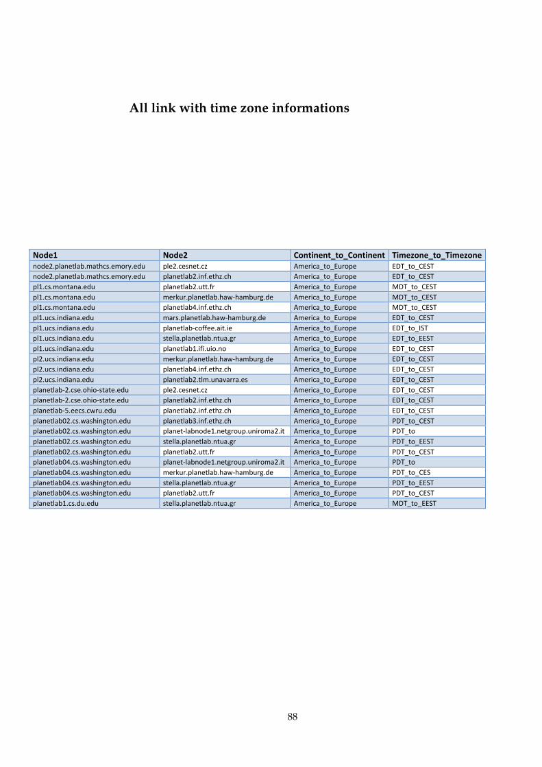
Node1   Node2   Continent_to_Continent   Timezone_to_Timezone  node2.planetlab.mathcs.emory.edu   ple2.cesnet.cz   America_to_Europe   EDT_to_CEST  node2.planetlab.mathcs.emory.edu   planetlab2.inf.ethz.ch   America_to_Europe   EDT_to_CEST  pl1.cs.montana.edu   planetlab2.utt.fr   America_to_Europe   MDT_to_CEST  pl1.cs.montana.edu   merkur.planetlab.haw-­‐hamburg.de   America_to_Europe   MDT_to_CEST  pl1.cs.montana.edu   planetlab4.inf.ethz.ch   America_to_Europe   MDT_to_CEST  pl1.ucs.indiana.edu   mars.planetlab.haw-­‐hamburg.de   America_to_Europe   EDT_to_CEST  pl1.ucs.indiana.edu   planetlab-­‐coffee.ait.ie   America_to_Europe   EDT_to_IST  pl1.ucs.indiana.edu   stella.planetlab.ntua.gr   America_to_Europe   EDT_to_EEST  pl1.ucs.indiana.edu   planetlab1.ifi.uio.no   America_to_Europe   EDT_to_CEST  pl2.ucs.indiana.edu   merkur.planetlab.haw-­‐hamburg.de   America_to_Europe   EDT_to_CEST  pl2.ucs.indiana.edu   planetlab4.inf.ethz.ch   America_to_Europe   EDT_to_CEST  pl2.ucs.indiana.edu   planetlab2.tlm.unavarra.es   America_to_Europe   EDT_to_CEST  planetlab-­‐2.cse.ohio-­‐state.edu   ple2.cesnet.cz   America_to_Europe   EDT_to_CEST  planetlab-­‐2.cse.ohio-­‐state.edu   planetlab2.inf.ethz.ch   America_to_Europe   EDT_to_CEST  planetlab-­‐5.eecs.cwru.edu   planetlab2.inf.ethz.ch   America_to_Europe   EDT_to_CEST  planetlab02.cs.washington.edu   planetlab3.inf.ethz.ch   America_to_Europe   PDT_to_CEST  planetlab02.cs.washington.edu   planet-­‐labnode1.netgroup.uniroma2.it   America_to_Europe   PDT_to  planetlab02.cs.washington.edu   stella.planetlab.ntua.gr   America_to_Europe   PDT_to_EEST  planetlab02.cs.washington.edu   planetlab2.utt.fr   America_to_Europe   PDT_to_CEST  planetlab04.cs.washington.edu   planet-­‐labnode1.netgroup.uniroma2.it   America_to_Europe   PDT_to  planetlab04.cs.washington.edu   merkur.planetlab.haw-­‐hamburg.de   America_to_Europe   PDT_to_CES  planetlab04.cs.washington.edu   stella.planetlab.ntua.gr   America_to_Europe   PDT_to_EEST  planetlab04.cs.washington.edu   planetlab2.utt.fr   America_to_Europe   PDT_to_CEST  planetlab1.cs.du.edu   stella.planetlab.ntua.gr   America_to_Europe   MDT_to_EEST  

All link with time zone informations

88

planetlab1.cs.du.edu   planetlab1.ifi.uio.no   America_to_Europe   MDT_to_CEST  planetlab1.cs.du.edu   planetlab2.utt.fr   America_to_Europe   MDT_to_CEST  planetlab1.cs.okstate.edu   planetlab2.cesnet.cz   America_to_Europe   CDT_to_CEST  planetlab1.cs.okstate.edu   planetlab1.ifi.uio.no   America_to_Europe   CDT_to_CEST  planetlab1.cs.okstate.edu   planetlab2.inf.ethz.ch   America_to_Europe   CDT_to_CEST  planetlab1.dtc.umn.edu   plab1.cs.msu.ru   America_to_Europe   CDT_to_EEST  planetlab1.dtc.umn.edu   planet-­‐labnode1.netgroup.uniroma2.it   America_to_Europe   CDT_to_CEST  planetlab1.pop-­‐mg.rnp.br   planetlab3.mini.pw.edu.pl   America_to_Europe   BRT_to_CEST  planetlab1.unr.edu   planetlab2.utt.fr   America_to_Europe   PDT_to_CEST  planetlab2.citadel.edu   planet-­‐labnode1.netgroup.uniroma2.it   America_to_Europe   EDT_to_CEST  planetlab2.citadel.edu   plab1.cs.msu.ru   America_to_Europe   EDT_to_EEST  planetlab2.cs.cornell.edu   ple2.cesnet.cz   America_to_Europe   EDT_to_CEST  planetlab2.cs.cornell.edu   planetlab2.inf.ethz.ch   America_to_Europe   EDT_to_CEST  planetlab2.cs.du.edu   planetlab1.ifi.uio.no   America_to_Europe   MDT_to_CEST  planetlab2.cs.du.edu   planetlab2.utt.fr   America_to_Europe   MDT_to_CEST  planetlab2.cs.du.edu   merkur.planetlab.haw-­‐hamburg.de   America_to_Europe   MDT_to_CEST  planetlab2.cs.du.edu   planetlab4.inf.ethz.ch   America_to_Europe   MDT_to_CEST  planetlab2.cs.ubc.ca   merkur.planetlab.haw-­‐hamburg.de   America_to_Europe   PDT_to_CEST  planetlab2.cs.ubc.ca   plab1.cs.msu.ru   America_to_Europe   PDT_to_EEST  planetlab2.cs.uoregon.edu   plab1.cs.msu.ru   America_to_Europe   PDT_to_EEST  planetlab2.cs.uoregon.edu   planet-­‐labnode1.netgroup.uniroma2.it   America_to_Europe   PDT_to_CES  planetlab2.cs.uoregon.edu   stella.planetlab.ntua.gr   America_to_Europe   PDT_to_EEST  planetlab2.pop-­‐mg.rnp.br   plab1.cs.msu.ru   America_to_Europe   BRT_to_EEST  planetlab2.utdallas.edu   stella.planetlab.ntua.gr   America_to_Europe   CDT_to_EEST  planetlab2.utdallas.edu   planetlab2.tlm.unavarra.es   America_to_Europe   CDT_to_CEST  

89

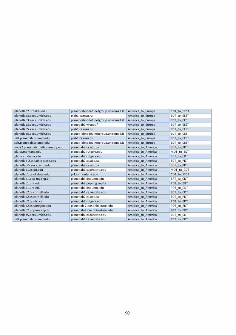
planetlab2.utdallas.edu   planet-­‐labnode1.netgroup.uniroma2.it   America_to_Europe   CDT_to_CEST  planetlab3.eecs.umich.edu   plab1.cs.msu.ru   America_to_Europe   EDT_to_EEST  planetlab3.eecs.umich.edu   planet-­‐labnode1.netgroup.uniroma2.it   America_to_Europe   EDT_to_CES  planetlab3.eecs.umich.edu   planetlab1.virtues.fi   America_to_Europe   EDT_to_EEST  planetlab5.eecs.umich.edu   plab1.cs.msu.ru   America_to_Europe   EDT_to_EEST  planetlab5.eecs.umich.edu   planet-­‐labnode1.netgroup.uniroma2.it   America_to_Europe   EDT_to_CES  salt.planetlab.cs.umd.edu   plab1.cs.msu.ru   America_to_Europe   EDT_to_EEST  salt.planetlab.cs.umd.edu   planet-­‐labnode1.netgroup.uniroma2.it   America_to_Europe   EDT_to_CEST  node2.planetlab.mathcs.emory.edu   planetlab2.cs.ubc.ca   America_to_America   EDT_to_PDT  pl1.cs.montana.edu   planetlab2.rutgers.edu   America_to_America   MDT_to_EDT  pl2.ucs.indiana.edu   planetlab2.rutgers.edu   America_to_America   EDT_to_EDT  planetlab-­‐2.cse.ohio-­‐state.edu   planetlab2.cs.ubc.ca   America_to_America   EDT_to_PDT  planetlab-­‐5.eecs.cwru.edu   planetlab2.cs.ubc.ca   America_to_America   EDT_to_PDT  planetlab1.cs.du.edu   planetlab1.cs.okstate.edu   America_to_America   MDT_to_CDT  planetlab1.cs.okstate.edu   pl1.cs.montana.edu   America_to_America   CDT_to_MDT  planetlab1.pop-­‐mg.rnp.br   planetlab1.dtc.umn.edu   America_to_America   BRT_to_CDT  planetlab1.unr.edu   planetlab2.pop-­‐mg.rnp.br   America_to_America   PDT_to_BRT  planetlab1.unr.edu   planetlab1.dtc.umn.edu   America_to_America   PDT_to_CDT  planetlab2.cs.cornell.edu   planetlab1.cs.okstate.edu   America_to_America   EDT_to_CDT  planetlab2.cs.cornell.edu   planetlab2.cs.ubc.ca   America_to_America   EDT_to_PDT  planetlab2.cs.ubc.ca   planetlab2.rutgers.edu   America_to_America   PDT_to_EDT  planetlab2.cs.uoregon.edu   planetlab-­‐2.cse.ohio-­‐state.edu   America_to_America   PDT_to_EDT  planetlab2.pop-­‐mg.rnp.br   planetlab-­‐2.cse.ohio-­‐state.edu   America_to_America   BRT_to_EDT  planetlab5.eecs.umich.edu   planetlab1.cs.okstate.edu   America_to_America   EDT_to_CDT  salt.planetlab.cs.umd.edu   planetlab1.cs.okstate.edu   America_to_America   EDT_to_CDT  

90

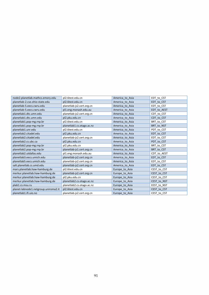
node2.planetlab.mathcs.emory.edu   pl2.6test.edu.cn   America_to_Asia   EDT_to_CST  planetlab-­‐2.cse.ohio-­‐state.edu   pl2.6test.edu.cn   America_to_Asia   EDT_to_CST  planetlab-­‐5.eecs.cwru.edu   planetlab-­‐js2.cert.org.cn   America_to_Asia   EDT_to_CST  planetlab-­‐5.eecs.cwru.edu   pl1.eng.monash.edu.au   America_to_Asia   EDT_to_AEST  planetlab1.dtc.umn.edu   planetlab-­‐js2.cert.org.cn   America_to_Asia   CDT_to_CST  planetlab1.dtc.umn.edu   pl2.pku.edu.cn   America_to_Asia   CDT_to_CST  planetlab1.pop-­‐mg.rnp.br   pl2.6test.edu.cn   America_to_Asia   BRT_to_CST  planetlab1.pop-­‐mg.rnp.br   planetlab1.cs.otago.ac.nz   America_to_Asia   BRT_to_NST  planetlab1.unr.edu   pl2.6test.edu.cn   America_to_Asia   PDT_to_CST  planetlab2.citadel.edu   pl2.pku.edu.cn   America_to_Asia   EDT_to_CST  planetlab2.citadel.edu   planetlab-­‐js2.cert.org.cn   America_to_Asia   EDT_to_CST  planetlab2.cs.ubc.ca   pl2.pku.edu.cn   America_to_Asia   PDT_to_CST  planetlab2.pop-­‐mg.rnp.br   pl2.pku.edu.cn   America_to_Asia   BRT_to_CST  planetlab2.pop-­‐mg.rnp.br   planetlab-­‐js1.cert.org.cn   America_to_Asia   BRT_to_CST  planetlab2.utdallas.edu   pl1.eng.monash.edu.au   America_to_Asia   CDT_to_AEST  planetlab3.eecs.umich.edu   planetlab-­‐js2.cert.org.cn   America_to_Asia   EDT_to_CST  planetlab5.eecs.umich.edu   planetlab-­‐js2.cert.org.cn   America_to_Asia   EDT_to_CST  salt.planetlab.cs.umd.edu   planetlab-­‐js2.cert.org.cn   America_to_Asia   EDT_to_CST  mars.planetlab.haw-­‐hamburg.de   pl2.6test.edu.cn   Europe_to_Asia   CEST_to_CST  merkur.planetlab.haw-­‐hamburg.de   planetlab-­‐js2.cert.org.cn   Europe_to_Asia   CEST_to_CST  merkur.planetlab.haw-­‐hamburg.de   pl2.pku.edu.cn   Europe_to_Asia   CEST_to_CST  merkur.planetlab.haw-­‐hamburg.de   planetlab2.cs.otago.ac.nz   Europe_to_Asia   CEST_to_NST  plab1.cs.msu.ru   planetlab2.cs.otago.ac.nz   Europe_to_Asia   EEST_to_NST  planet-­‐labnode1.netgroup.uniroma2.it   pl2.6test.edu.cn   Europe_to_Asia   CEST_to_CST  planetlab1.ifi.uio.no   planetlab-­‐js2.cert.org.cn   Europe_to_Asia   CEST_to_CST  

91

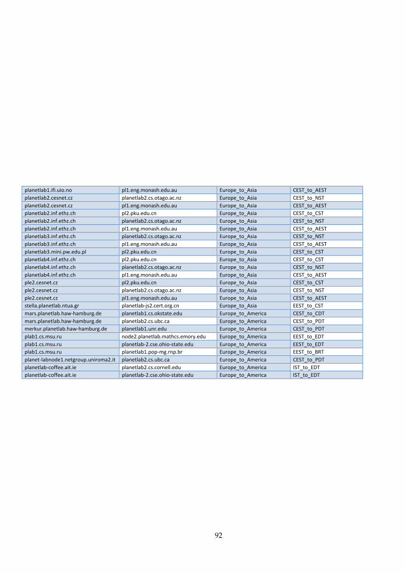
planetlab1.ifi.uio.no   pl1.eng.monash.edu.au   Europe_to_Asia   CEST_to_AEST  planetlab2.cesnet.cz   planetlab2.cs.otago.ac.nz   Europe_to_Asia   CEST_to_NST  planetlab2.cesnet.cz   pl1.eng.monash.edu.au   Europe_to_Asia   CEST_to_AEST  planetlab2.inf.ethz.ch   pl2.pku.edu.cn   Europe_to_Asia   CEST_to_CST  planetlab2.inf.ethz.ch   planetlab2.cs.otago.ac.nz   Europe_to_Asia   CEST_to_NST  planetlab2.inf.ethz.ch   pl1.eng.monash.edu.au   Europe_to_Asia   CEST_to_AEST  planetlab3.inf.ethz.ch   planetlab2.cs.otago.ac.nz   Europe_to_Asia   CEST_to_NST  planetlab3.inf.ethz.ch   pl1.eng.monash.edu.au   Europe_to_Asia   CEST_to_AEST  planetlab3.mini.pw.edu.pl   pl2.pku.edu.cn   Europe_to_Asia   CEST_to_CST  planetlab4.inf.ethz.ch   pl2.pku.edu.cn   Europe_to_Asia   CEST_to_CST  planetlab4.inf.ethz.ch   planetlab2.cs.otago.ac.nz   Europe_to_Asia   CEST_to_NST  planetlab4.inf.ethz.ch   pl1.eng.monash.edu.au   Europe_to_Asia   CEST_to_AEST  ple2.cesnet.cz   pl2.pku.edu.cn   Europe_to_Asia   CEST_to_CST  ple2.cesnet.cz   planetlab2.cs.otago.ac.nz   Europe_to_Asia   CEST_to_NST  ple2.cesnet.cz   pl1.eng.monash.edu.au   Europe_to_Asia   CEST_to_AEST  stella.planetlab.ntua.gr   planetlab-­‐js2.cert.org.cn   Europe_to_Asia   EEST_to_CST  mars.planetlab.haw-­‐hamburg.de   planetlab1.cs.okstate.edu   Europe_to_America   CEST_to_CDT  mars.planetlab.haw-­‐hamburg.de   planetlab2.cs.ubc.ca   Europe_to_America   CEST_to_PDT  merkur.planetlab.haw-­‐hamburg.de   planetlab1.unr.edu   Europe_to_America   CEST_to_PDT  plab1.cs.msu.ru   node2.planetlab.mathcs.emory.edu   Europe_to_America   EEST_to_EDT  plab1.cs.msu.ru   planetlab-­‐2.cse.ohio-­‐state.edu   Europe_to_America   EEST_to_EDT  plab1.cs.msu.ru   planetlab1.pop-­‐mg.rnp.br   Europe_to_America   EEST_to_BRT  planet-­‐labnode1.netgroup.uniroma2.it   planetlab2.cs.ubc.ca   Europe_to_America   CEST_to_PDT  planetlab-­‐coffee.ait.ie   planetlab2.cs.cornell.edu   Europe_to_America   IST_to_EDT  planetlab-­‐coffee.ait.ie   planetlab-­‐2.cse.ohio-­‐state.edu   Europe_to_America   IST_to_EDT  

92

planetlab-­‐coffee.ait.ie   planetlab1.cs.okstate.edu   Europe_to_America   IST_to_CDT  planetlab-­‐coffee.ait.ie   planetlab1.unr.edu   Europe_to_America   IST_to_PDT  planetlab1.cesnet.cz   planetlab04.cs.washington.edu   Europe_to_America   CEST_to_PDT  planetlab1.cesnet.cz   planetlab1.cs.okstate.edu   Europe_to_America   CEST_to_CDT  planetlab1.ifi.uio.no   planetlab2.rutgers.edu   Europe_to_America   CEST_to_EDT  planetlab1.ifi.uio.no   planetlab2.citadel.edu   Europe_to_America   CEST_to_EDT  planetlab1.net.in.tum.de   planetlab04.cs.washington.edu   Europe_to_America   CEST_to_PDT  planetlab1.net.in.tum.de   planetlab2.rutgers.edu   Europe_to_America   CEST_to_EDT  planetlab1.net.in.tum.de   planetlab2.pop-­‐mg.rnp.br   Europe_to_America   CEST_to_BRT  planetlab1.net.in.tum.de   pl1.cs.montana.edu   Europe_to_America   CEST_to_MDT  planetlab1.virtues.fi   planetlab2.pop-­‐mg.rnp.br   Europe_to_America   EEST_to_BRT  planetlab1.virtues.fi   planetlab1.unr.edu   Europe_to_America   EEST_to_PDT  planetlab1.virtues.fi   planetlab2.cs.cornell.edu   Europe_to_America   EEST_to_EDT  planetlab2.cesnet.cz   planetlab2.rutgers.edu   Europe_to_America   CEST_to_EDT  planetlab2.cesnet.cz   planetlab2.cs.ubc.ca   Europe_to_America   CEST_to_PDT  planetlab2.tlm.unavarra.es   planetlab1.dtc.umn.edu   Europe_to_America   CEST_to_CDT  planetlab2.tlm.unavarra.es   planetlab04.cs.washington.edu   Europe_to_America   CEST_to_PDT  planetlab2.tlm.unavarra.es   planetlab1.cs.okstate.edu   Europe_to_America   CEST_to_CDT  planetlab2.utt.fr   planetlab1.cs.okstate.edu   Europe_to_America   CEST_to_CDT  planetlab2.utt.fr   planetlab2.cs.ubc.ca   Europe_to_America   CEST_to_PDT  planetlab3.cesnet.cz   planetlab04.cs.washington.edu   Europe_to_America   CEST_to_PDT  planetlab3.cesnet.cz   planetlab2.rutgers.edu   Europe_to_America   CEST_to_EDT  planetlab3.cesnet.cz   pl1.cs.montana.edu   Europe_to_America   CEST_to_MDT  planetlab3.inf.ethz.ch   planetlab2.cs.du.edu   Europe_to_America   CEST_to_MDT  planetlab3.mini.pw.edu.pl   planetlab-­‐2.cse.ohio-­‐state.edu   Europe_to_America   CEST_to_EDT  

93

planetlab3.mini.pw.edu.pl   planetlab2.cs.ubc.ca   Europe_to_America   CEST_to_PDT  planetlab3.mini.pw.edu.pl   planetlab-­‐5.eecs.cwru.edu   Europe_to_America   CEST_to_EDT  planetlab4.mini.pw.edu.pl   planetlab-­‐2.cse.ohio-­‐state.edu   Europe_to_America   CEST_to_EDT  planetlab4.mini.pw.edu.pl   planetlab-­‐5.eecs.cwru.edu   Europe_to_America   CEST_to_EDT  planetlab4.mini.pw.edu.pl   pl2.ucs.indiana.edu   Europe_to_America   CEST_to_EDT  planetlab4.mini.pw.edu.pl   planetlab2.citadel.edu   Europe_to_America   CEST_to_EDT  ple2.cesnet.cz   planetlab1.cs.okstate.edu   Europe_to_America   CEST_to_CDT  stella.planetlab.ntua.gr   planetlab2.cs.ubc.ca   Europe_to_America   EEST_to_PDT  mars.planetlab.haw-­‐hamburg.de   planetlab2.inf.ethz.ch   Europe_to_Europe   CEST_to_CEST  planet-­‐labnode1.netgroup.uniroma2.it   ple2.cesnet.cz   Europe_to_Europe   CEST_to_CEST  planet-­‐labnode1.netgroup.uniroma2.it   planetlab2.inf.ethz.ch   Europe_to_Europe   CEST_to_CEST  planetlab1.cesnet.cz   planetlab1.ifi.uio.no   Europe_to_Europe   CEST_to_CEST  planetlab1.cesnet.cz   planetlab2.utt.fr   Europe_to_Europe   CEST_to_CEST  planetlab1.virtues.fi   planetlab2.tlm.unavarra.es   Europe_to_Europe   EEST_to_CEST  planetlab2.inf.ethz.ch   planetlab1.ifi.uio.no   Europe_to_Europe   CEST_to_CEST  planetlab2.tlm.unavarra.es   planetlab1.ifi.uio.no   Europe_to_Europe   CEST_to_CEST  planetlab2.utt.fr   ple2.cesnet.cz   Europe_to_Europe   CEST_to_CEST  planetlab2.utt.fr   planetlab2.inf.ethz.ch   Europe_to_Europe   CEST_to_CEST  planetlab3.cesnet.cz   planetlab2.utt.fr   Europe_to_Europe   CEST_to_CEST  planetlab3.inf.ethz.ch   planetlab1.ifi.uio.no   Europe_to_Europe   CEST_to_CEST  planetlab4.inf.ethz.ch   planetlab1.ifi.uio.no   Europe_to_Europe   CEST_to_CEST  stella.planetlab.ntua.gr   ple2.cesnet.cz   Europe_to_Europe   EEST_to_CEST  stella.planetlab.ntua.gr   planetlab2.inf.ethz.ch   Europe_to_Europe   EEST_to_CEST  pl1.eng.monash.edu.au   stella.planetlab.ntua.gr   Asia_to_Europe   AEST_to_EEST  pl2.6test.edu.cn   plab1.cs.msu.ru   Asia_to_Europe   CST_to_EEST  

94

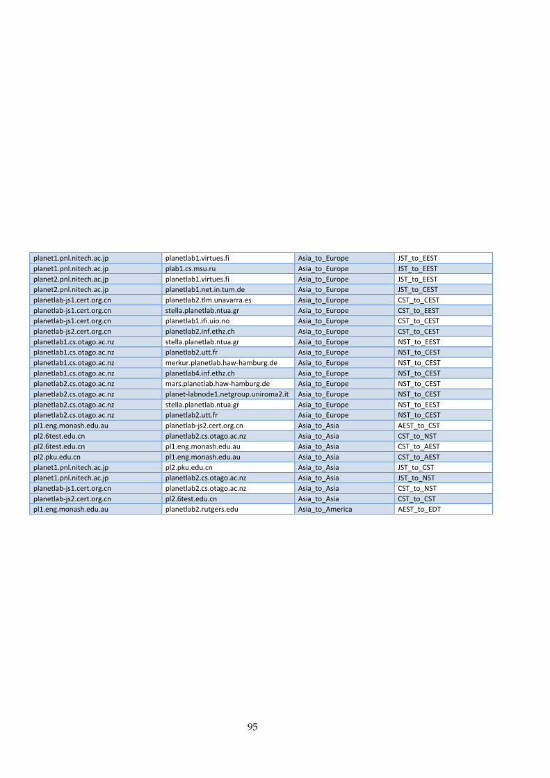
planet1.pnl.nitech.ac.jp   planetlab1.virtues.fi   Asia_to_Europe   JST_to_EEST  planet1.pnl.nitech.ac.jp   plab1.cs.msu.ru   Asia_to_Europe   JST_to_EEST  planet2.pnl.nitech.ac.jp   planetlab1.virtues.fi   Asia_to_Europe   JST_to_EEST  planet2.pnl.nitech.ac.jp   planetlab1.net.in.tum.de   Asia_to_Europe   JST_to_CEST  planetlab-­‐js1.cert.org.cn   planetlab2.tlm.unavarra.es   Asia_to_Europe   CST_to_CEST  planetlab-­‐js1.cert.org.cn   stella.planetlab.ntua.gr   Asia_to_Europe   CST_to_EEST  planetlab-­‐js1.cert.org.cn   planetlab1.ifi.uio.no   Asia_to_Europe   CST_to_CEST  planetlab-­‐js2.cert.org.cn   planetlab2.inf.ethz.ch   Asia_to_Europe   CST_to_CEST  planetlab1.cs.otago.ac.nz   stella.planetlab.ntua.gr   Asia_to_Europe   NST_to_EEST  planetlab1.cs.otago.ac.nz   planetlab2.utt.fr   Asia_to_Europe   NST_to_CEST  planetlab1.cs.otago.ac.nz   merkur.planetlab.haw-­‐hamburg.de   Asia_to_Europe   NST_to_CEST  planetlab1.cs.otago.ac.nz   planetlab4.inf.ethz.ch   Asia_to_Europe   NST_to_CEST  planetlab2.cs.otago.ac.nz   mars.planetlab.haw-­‐hamburg.de   Asia_to_Europe   NST_to_CEST  planetlab2.cs.otago.ac.nz   planet-­‐labnode1.netgroup.uniroma2.it   Asia_to_Europe   NST_to_CEST  planetlab2.cs.otago.ac.nz   stella.planetlab.ntua.gr   Asia_to_Europe   NST_to_EEST  planetlab2.cs.otago.ac.nz   planetlab2.utt.fr   Asia_to_Europe   NST_to_CEST  pl1.eng.monash.edu.au   planetlab-­‐js2.cert.org.cn   Asia_to_Asia   AEST_to_CST  pl2.6test.edu.cn   planetlab2.cs.otago.ac.nz   Asia_to_Asia   CST_to_NST  pl2.6test.edu.cn   pl1.eng.monash.edu.au   Asia_to_Asia   CST_to_AEST  pl2.pku.edu.cn   pl1.eng.monash.edu.au   Asia_to_Asia   CST_to_AEST  planet1.pnl.nitech.ac.jp   pl2.pku.edu.cn   Asia_to_Asia   JST_to_CST  planet1.pnl.nitech.ac.jp   planetlab2.cs.otago.ac.nz   Asia_to_Asia   JST_to_NST  planetlab-­‐js1.cert.org.cn   planetlab2.cs.otago.ac.nz   Asia_to_Asia   CST_to_NST  planetlab-­‐js2.cert.org.cn   pl2.6test.edu.cn   Asia_to_Asia   CST_to_CST  pl1.eng.monash.edu.au   planetlab2.rutgers.edu   Asia_to_America   AEST_to_EDT  

95

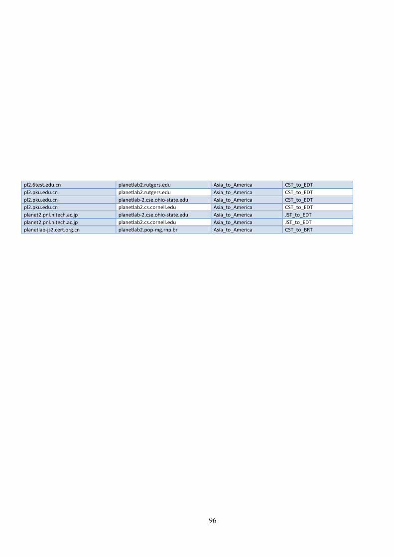
pl2.6test.edu.cn   planetlab2.rutgers.edu   Asia_to_America   CST_to_EDT  pl2.pku.edu.cn   planetlab2.rutgers.edu   Asia_to_America   CST_to_EDT  pl2.pku.edu.cn   planetlab-­‐2.cse.ohio-­‐state.edu   Asia_to_America   CST_to_EDT  pl2.pku.edu.cn   planetlab2.cs.cornell.edu   Asia_to_America   CST_to_EDT  planet2.pnl.nitech.ac.jp   planetlab-­‐2.cse.ohio-­‐state.edu   Asia_to_America   JST_to_EDT  planet2.pnl.nitech.ac.jp   planetlab2.cs.cornell.edu   Asia_to_America   JST_to_EDT  planetlab-­‐js2.cert.org.cn   planetlab2.pop-­‐mg.rnp.br   Asia_to_America   CST_to_BRT    

96

Correlated Traceroute Result

97

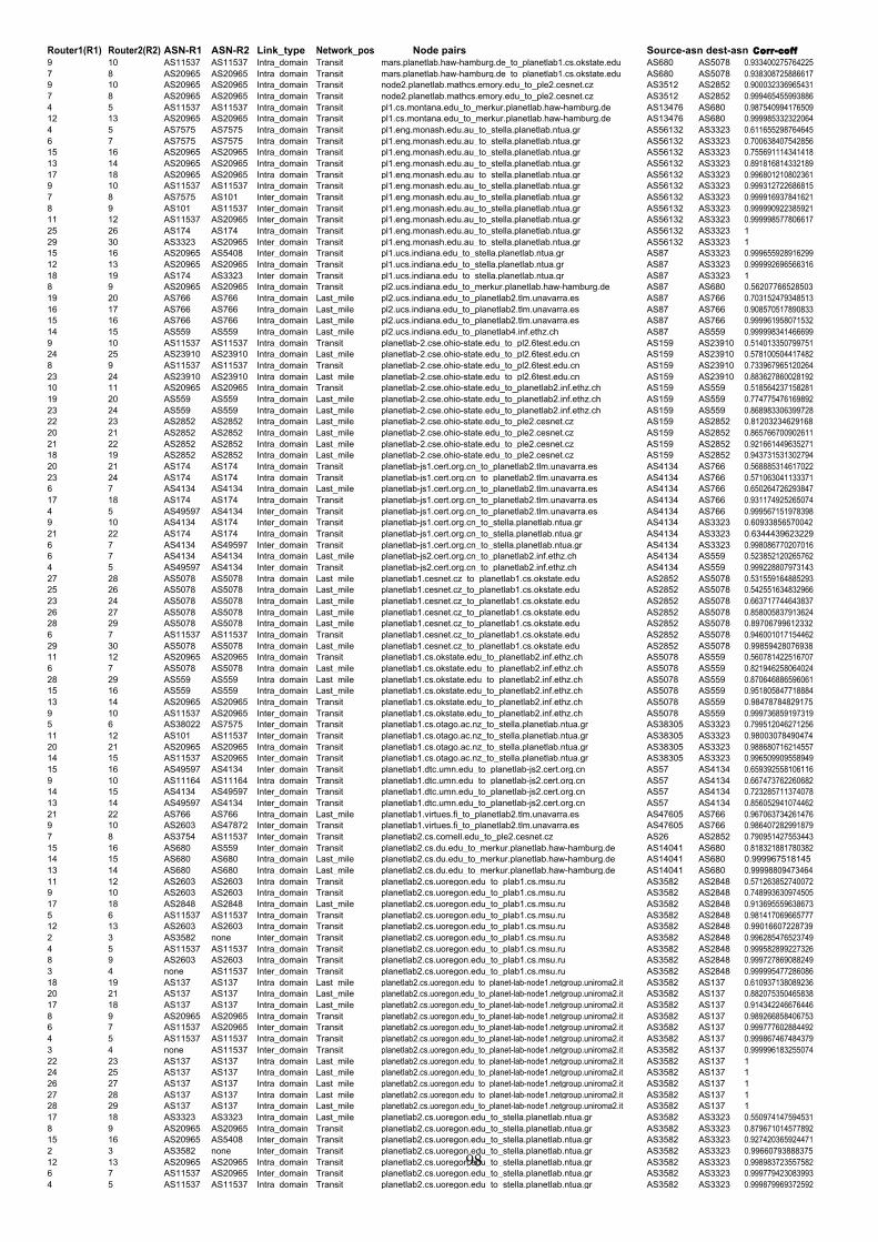
Router1(R1) Router2(R2) ASN-R1 ASN-R2 Link_type Network_pos Node pairs 9 10 AS11537 AS11537 Intra_domain Transit mars.planetlab.haw-hamburg.de_to_planetlab1.cs.okstate.edu 7 8 AS20965 AS20965 Intra_domain Transit mars.planetlab.haw-hamburg.de_to_planetlab1.cs.okstate.edu 9 10 AS20965 AS20965 Intra_domain Transit node2.planetlab.mathcs.emory.edu_to_ple2.cesnet.cz 7 8 AS20965 AS20965 Intra_domain Transit node2.planetlab.mathcs.emory.edu_to_ple2.cesnet.cz 4 5 AS11537 AS11537 Intra_domain Transit pl1.cs.montana.edu_to_merkur.planetlab.haw-hamburg.de 12 13 AS20965 AS20965 Intra_domain Transit pl1.cs.montana.edu_to_merkur.planetlab.haw-hamburg.de 4 5 AS7575 AS7575 Intra_domain Transit pl1.eng.monash.edu.au_to_stella.planetlab.ntua.gr 6 7 AS7575 AS7575 Intra_domain Transit pl1.eng.monash.edu.au_to_stella.planetlab.ntua.gr 15 16 AS20965 AS20965 Intra_domain Transit pl1.eng.monash.edu.au_to_stella.planetlab.ntua.gr 13 14 AS20965 AS20965 Intra_domain Transit pl1.eng.monash.edu.au_to_stella.planetlab.ntua.gr 17 18 AS20965 AS20965 Intra_domain Transit pl1.eng.monash.edu.au_to_stella.planetlab.ntua.gr 9 10 AS11537 AS11537 Intra_domain Transit pl1.eng.monash.edu.au_to_stella.planetlab.ntua.gr 7 8 AS7575 AS101 Inter_domain Transit pl1.eng.monash.edu.au_to_stella.planetlab.ntua.gr 8 9 AS101 AS11537 Inter_domain Transit pl1.eng.monash.edu.au_to_stella.planetlab.ntua.gr 11 12 AS11537 AS20965 Inter_domain Transit pl1.eng.monash.edu.au_to_stella.planetlab.ntua.gr 25 26 AS174 AS174 Intra_domain Transit pl1.eng.monash.edu.au_to_stella.planetlab.ntua.gr 29 30 AS3323 AS20965 Inter_domain Transit pl1.eng.monash.edu.au_to_stella.planetlab.ntua.gr 15 16 AS20965 AS5408 Inter_domain Transit pl1.ucs.indiana.edu_to_stella.planetlab.ntua.gr 12 13 AS20965 AS20965 Intra_domain Transit pl1.ucs.indiana.edu_to_stella.planetlab.ntua.gr 18 19 AS174 AS3323 Inter_domain Transit pl1.ucs.indiana.edu_to_stella.planetlab.ntua.gr 8 9 AS20965 AS20965 Intra_domain Transit pl2.ucs.indiana.edu_to_merkur.planetlab.haw-hamburg.de 19 20 AS766 AS766 Intra_domain Last_mile pl2.ucs.indiana.edu_to_planetlab2.tlm.unavarra.es 16 17 AS766 AS766 Intra_domain Last_mile pl2.ucs.indiana.edu_to_planetlab2.tlm.unavarra.es 15 16 AS766 AS766 Intra_domain Last_mile pl2.ucs.indiana.edu_to_planetlab2.tlm.unavarra.es 14 15 AS559 AS559 Intra_domain Last_mile pl2.ucs.indiana.edu_to_planetlab4.inf.ethz.ch 9 10 AS11537 AS11537 Intra_domain Transit planetlab-2.cse.ohio-state.edu_to_pl2.6test.edu.cn 24 25 AS23910 AS23910 Intra_domain Last_mile planetlab-2.cse.ohio-state.edu_to_pl2.6test.edu.cn 8 9 AS11537 AS11537 Intra_domain Transit planetlab-2.cse.ohio-state.edu_to_pl2.6test.edu.cn 23 24 AS23910 AS23910 Intra_domain Last_mile planetlab-2.cse.ohio-state.edu_to_pl2.6test.edu.cn 10 11 AS20965 AS20965 Intra_domain Transit planetlab-2.cse.ohio-state.edu_to_planetlab2.inf.ethz.ch 19 20 AS559 AS559 Intra_domain Last_mile planetlab-2.cse.ohio-state.edu_to_planetlab2.inf.ethz.ch 23 24 AS559 AS559 Intra_domain Last_mile planetlab-2.cse.ohio-state.edu_to_planetlab2.inf.ethz.ch 22 23 AS2852 AS2852 Intra_domain Last_mile planetlab-2.cse.ohio-state.edu_to_ple2.cesnet.cz 20 21 AS2852 AS2852 Intra_domain Last_mile planetlab-2.cse.ohio-state.edu_to_ple2.cesnet.cz 21 22 AS2852 AS2852 Intra_domain Last_mile planetlab-2.cse.ohio-state.edu_to_ple2.cesnet.cz 18 19 AS2852 AS2852 Intra_domain Last_mile planetlab-2.cse.ohio-state.edu_to_ple2.cesnet.cz 20 21 AS174 AS174 Intra_domain Transit planetlab-js1.cert.org.cn_to_planetlab2.tlm.unavarra.es 23 24 AS174 AS174 Intra_domain Transit planetlab-js1.cert.org.cn_to_planetlab2.tlm.unavarra.es 6 7 AS4134 AS4134 Intra_domain Last_mile planetlab-js1.cert.org.cn_to_planetlab2.tlm.unavarra.es 17 18 AS174 AS174 Intra_domain Transit planetlab-js1.cert.org.cn_to_planetlab2.tlm.unavarra.es 4 5 AS49597 AS4134 Inter_domain Transit planetlab-js1.cert.org.cn_to_planetlab2.tlm.unavarra.es 9 10 AS4134 AS174 Inter_domain Transit planetlab-js1.cert.org.cn_to_stella.planetlab.ntua.gr 21 22 AS174 AS174 Intra_domain Transit planetlab-js1.cert.org.cn_to_stella.planetlab.ntua.gr 6 7 AS4134 AS49597 Inter_domain Transit planetlab-js1.cert.org.cn_to_stella.planetlab.ntua.gr 6 7 AS4134 AS4134 Intra_domain Last_mile planetlab-js2.cert.org.cn_to_planetlab2.inf.ethz.ch 4 5 AS49597 AS4134 Inter_domain Transit planetlab-js2.cert.org.cn_to_planetlab2.inf.ethz.ch 27 28 AS5078 AS5078 Intra_domain Last_mile planetlab1.cesnet.cz_to_planetlab1.cs.okstate.edu 25 26 AS5078 AS5078 Intra_domain Last_mile planetlab1.cesnet.cz_to_planetlab1.cs.okstate.edu 23 24 AS5078 AS5078 Intra_domain Last_mile planetlab1.cesnet.cz_to_planetlab1.cs.okstate.edu 26 27 AS5078 AS5078 Intra_domain Last_mile planetlab1.cesnet.cz_to_planetlab1.cs.okstate.edu 28 29 AS5078 AS5078 Intra_domain Last_mile planetlab1.cesnet.cz_to_planetlab1.cs.okstate.edu 6 7 AS11537 AS11537 Intra_domain Transit planetlab1.cesnet.cz_to_planetlab1.cs.okstate.edu 29 30 AS5078 AS5078 Intra_domain Last_mile planetlab1.cesnet.cz_to_planetlab1.cs.okstate.edu 11 12 AS20965 AS20965 Intra_domain Transit planetlab1.cs.okstate.edu_to_planetlab2.inf.ethz.ch 6 7 AS5078 AS5078 Intra_domain Last_mile planetlab1.cs.okstate.edu_to_planetlab2.inf.ethz.ch 28 29 AS559 AS559 Intra_domain Last_mile planetlab1.cs.okstate.edu_to_planetlab2.inf.ethz.ch 15 16 AS559 AS559 Intra_domain Last_mile planetlab1.cs.okstate.edu_to_planetlab2.inf.ethz.ch 13 14 AS20965 AS20965 Intra_domain Transit planetlab1.cs.okstate.edu_to_planetlab2.inf.ethz.ch 9 10 AS11537 AS20965 Inter_domain Transit planetlab1.cs.okstate.edu_to_planetlab2.inf.ethz.ch 5 6 AS38022 AS7575 Inter_domain Transit planetlab1.cs.otago.ac.nz_to_stella.planetlab.ntua.gr 11 12 AS101 AS11537 Inter_domain Transit planetlab1.cs.otago.ac.nz_to_stella.planetlab.ntua.gr 20 21 AS20965 AS20965 Intra_domain Transit planetlab1.cs.otago.ac.nz_to_stella.planetlab.ntua.gr 14 15 AS11537 AS20965 Inter_domain Transit planetlab1.cs.otago.ac.nz_to_stella.planetlab.ntua.gr 15 16 AS49597 AS4134 Inter_domain Transit planetlab1.dtc.umn.edu_to_planetlab-js2.cert.org.cn 9 10 AS11164 AS11164 Intra_domain Transit planetlab1.dtc.umn.edu_to_planetlab-js2.cert.org.cn 14 15 AS4134 AS49597 Inter_domain Transit planetlab1.dtc.umn.edu_to_planetlab-js2.cert.org.cn 13 14 AS49597 AS4134 Inter_domain Transit planetlab1.dtc.umn.edu_to_planetlab-js2.cert.org.cn 21 22 AS766 AS766 Intra_domain Last_mile planetlab1.virtues.fi_to_planetlab2.tlm.unavarra.es 9 10 AS2603 AS47872 Inter_domain Transit planetlab1.virtues.fi_to_planetlab2.tlm.unavarra.es 7 8 AS3754 AS11537 Inter_domain Transit planetlab2.cs.cornell.edu_to_ple2.cesnet.cz 15 16 AS680 AS559 Inter_domain Transit planetlab2.cs.du.edu_to_merkur.planetlab.haw-hamburg.de 14 15 AS680 AS680 Intra_domain Last_mile planetlab2.cs.du.edu_to_merkur.planetlab.haw-hamburg.de 13 14 AS680 AS680 Intra_domain Last_mile planetlab2.cs.du.edu_to_merkur.planetlab.haw-hamburg.de 11 12 AS2603 AS2603 Intra_domain Transit planetlab2.cs.uoregon.edu_to_plab1.cs.msu.ru 9 10 AS2603 AS2603 Intra_domain Transit planetlab2.cs.uoregon.edu_to_plab1.cs.msu.ru 17 18 AS2848 AS2848 Intra_domain Last_mile planetlab2.cs.uoregon.edu_to_plab1.cs.msu.ru 5 6 AS11537 AS11537 Intra_domain Transit planetlab2.cs.uoregon.edu_to_plab1.cs.msu.ru 12 13 AS2603 AS2603 Intra_domain Transit planetlab2.cs.uoregon.edu_to_plab1.cs.msu.ru 2 3 AS3582 none Inter_domain Transit planetlab2.cs.uoregon.edu_to_plab1.cs.msu.ru 4 5 AS11537 AS11537 Intra_domain Transit planetlab2.cs.uoregon.edu_to_plab1.cs.msu.ru 8 9 AS2603 AS2603 Intra_domain Transit planetlab2.cs.uoregon.edu_to_plab1.cs.msu.ru 3 4 none AS11537 Inter_domain Transit planetlab2.cs.uoregon.edu_to_plab1.cs.msu.ru 18 19 AS137 AS137 Intra_domain Last_mile planetlab2.cs.uoregon.edu_to_planet-lab-node1.netgroup.uniroma2.it 20 21 AS137 AS137 Intra_domain Last_mile planetlab2.cs.uoregon.edu_to_planet-lab-node1.netgroup.uniroma2.it 17 18 AS137 AS137 Intra_domain Last_mile planetlab2.cs.uoregon.edu_to_planet-lab-node1.netgroup.uniroma2.it 8 9 AS20965 AS20965 Intra_domain Transit planetlab2.cs.uoregon.edu_to_planet-lab-node1.netgroup.uniroma2.it 6 7 AS11537 AS20965 Inter_domain Transit planetlab2.cs.uoregon.edu_to_planet-lab-node1.netgroup.uniroma2.it 4 5 AS11537 AS11537 Intra_domain Transit planetlab2.cs.uoregon.edu_to_planet-lab-node1.netgroup.uniroma2.it 3 4 none AS11537 Inter_domain Transit planetlab2.cs.uoregon.edu_to_planet-lab-node1.netgroup.uniroma2.it 22 23 AS137 AS137 Intra_domain Last_mile planetlab2.cs.uoregon.edu_to_planet-lab-node1.netgroup.uniroma2.it 24 25 AS137 AS137 Intra_domain Last_mile planetlab2.cs.uoregon.edu_to_planet-lab-node1.netgroup.uniroma2.it 26 27 AS137 AS137 Intra_domain Last_mile planetlab2.cs.uoregon.edu_to_planet-lab-node1.netgroup.uniroma2.it 27 28 AS137 AS137 Intra_domain Last_mile planetlab2.cs.uoregon.edu_to_planet-lab-node1.netgroup.uniroma2.it 28 29 AS137 AS137 Intra_domain Last_mile planetlab2.cs.uoregon.edu_to_planet-lab-node1.netgroup.uniroma2.it 17 18 AS3323 AS3323 Intra_domain Last_mile planetlab2.cs.uoregon.edu_to_stella.planetlab.ntua.gr 8 9 AS20965 AS20965 Intra_domain Transit planetlab2.cs.uoregon.edu_to_stella.planetlab.ntua.gr 15 16 AS20965 AS5408 Inter_domain Transit planetlab2.cs.uoregon.edu_to_stella.planetlab.ntua.gr 2 3 AS3582 none Inter_domain Transit planetlab2.cs.uoregon.edu_to_stella.planetlab.ntua.gr 12 13 AS20965 AS20965 Intra_domain Transit planetlab2.cs.uoregon.edu_to_stella.planetlab.ntua.gr 6 7 AS11537 AS20965 Inter_domain Transit planetlab2.cs.uoregon.edu_to_stella.planetlab.ntua.gr 4 5 AS11537 AS11537 Intra_domain Transit planetlab2.cs.uoregon.edu_to_stella.planetlab.ntua.gr

Source-asn dest-asn Corr-coff AS680 AS5078 0.933400275764225 AS680 AS5078 0.938308725886617 AS3512 AS2852 0.900032336965431 AS3512 AS2852 0.999465455993886 AS13476 AS680 0.987540994176509 AS13476 AS680 0.999985332322064 AS56132 AS3323 0.611655298764645 AS56132 AS3323 0.700638407542856 AS56132 AS3323 0.755691114341418 AS56132 AS3323 0.891816814332189 AS56132 AS3323 0.996801210802361 AS56132 AS3323 0.999312722686815 AS56132 AS3323 0.999916937841621 AS56132 AS3323 0.999990922385921 AS56132 AS3323 0.999998577806617 AS56132 AS3323 1 AS56132 AS3323 1 AS87 AS3323 0.999655928916299 AS87 AS3323 0.999992696566316 AS87 AS3323 1 AS87 AS680 0.56207766528503 AS87 AS766 0.703152479348513 AS87 AS766 0.908570517890833 AS87 AS766 0.999961958071532 AS87 AS559 0.999998341466699 AS159 AS23910 0.514013350799751 AS159 AS23910 0.578100504417482 AS159 AS23910 0.733967965120264 AS159 AS23910 0.883627860028192 AS159 AS559 0.518564237158281 AS159 AS559 0.774775476169892 AS159 AS559 0.868983306399728 AS159 AS2852 0.81203234629168 AS159 AS2852 0.865766700902611 AS159 AS2852 0.921661449635271 AS159 AS2852 0.943731531302794 AS4134 AS766 0.568885314617022 AS4134 AS766 0.571063041133371 AS4134 AS766 0.650264726293847 AS4134 AS766 0.931174925265074 AS4134 AS766 0.999567151978398 AS4134 AS3323 0.60933856570042 AS4134 AS3323 0.6344439623229 AS4134 AS3323 0.998086770207016 AS4134 AS559 0.523852120265762 AS4134 AS559 0.999228807973143 AS2852 AS5078 0.531559164885293 AS2852 AS5078 0.542551634832966 AS2852 AS5078 0.663717744643837 AS2852 AS5078 0.858005837913624 AS2852 AS5078 0.89706799612332 AS2852 AS5078 0.946001017154462 AS2852 AS5078 0.99859428076938 AS5078 AS559 0.560781422516707 AS5078 AS559 0.821946258064024 AS5078 AS559 0.870646886596061 AS5078 AS559 0.951805847718884 AS5078 AS559 0.98478784829175 AS5078 AS559 0.999736859197319 AS38305 AS3323 0.799512046271256 AS38305 AS3323 0.98003078490474 AS38305 AS3323 0.988680716214557 AS38305 AS3323 0.996509909558949 AS57 AS4134 0.659392558106116 AS57 AS4134 0.667473762260682 AS57 AS4134 0.723285711374078 AS57 AS4134 0.856052941074462 AS47605 AS766 0.967063734261476 AS47605 AS766 0.986407282991879 AS26 AS2852 0.790951427553443 AS14041 AS680 0.818321881780382 AS14041 AS680 0.999967518145 AS14041 AS680 0.99998809473464 AS3582 AS2848 0.571263852740072 AS3582 AS2848 0.748993630974505 AS3582 AS2848 0.913695559638673 AS3582 AS2848 0.981417069665777 AS3582 AS2848 0.99016607228739 AS3582 AS2848 0.996285476523749 AS3582 AS2848 0.999582899227326 AS3582 AS2848 0.999727869088249 AS3582 AS2848 0.999995477286086 AS3582 AS137 0.610937138089236 AS3582 AS137 0.882075350465838 AS3582 AS137 0.914342246676446 AS3582 AS137 0.989266858406753 AS3582 AS137 0.999777602884492 AS3582 AS137 0.999867467484379 AS3582 AS137 0.999996183255074 AS3582 AS137 1 AS3582 AS137 1 AS3582 AS137 1 AS3582 AS137 1 AS3582 AS137 1 AS3582 AS3323 0.550974147594531 AS3582 AS3323 0.879671014577892 AS3582 AS3323 0.927420365924471 AS3582 AS3323 0.99660793888375 AS3582 AS3323 0.998983723557582 AS3582 AS3323 0.999779423083993 AS3582 AS3323 0.999879969372592

98

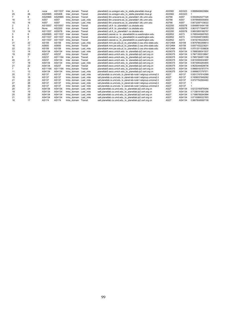
3 4 none AS11537 Inter_domain Transit planetlab2.cs.uoregon.edu_to_stella.planetlab.ntua.gr 25 26 AS20965 AS5408 Inter_domain Transit planetlab2.cs.uoregon.edu_to_stella.planetlab.ntua.gr 7 8 AS20965 AS20965 Intra_domain Transit planetlab2.tlm.unavarra.es_to_planetlab1.dtc.umn.edu 16 17 AS57 AS57 Intra_domain Last_mile planetlab2.tlm.unavarra.es_to_planetlab1.dtc.umn.edu 15 16 AS57 AS57 Intra_domain Last_mile planetlab2.tlm.unavarra.es_to_planetlab1.dtc.umn.edu 2 3 AS15557 AS15557 Intra_domain Transit planetlab2.utt.fr_to_planetlab1.cs.okstate.edu 5 6 None AS2200 Inter_domain Transit planetlab2.utt.fr_to_planetlab1.cs.okstate.edu 13 14 AS11537 AS5078 Inter_domain Transit planetlab2.utt.fr_to_planetlab1.cs.okstate.edu 5 6 AS20965 AS11537 Inter_domain Transit planetlab3.cesnet.cz_to_planetlab04.cs.washington.edu 8 9 AS11537 AS11537 Intra_domain Transit planetlab3.cesnet.cz_to_planetlab04.cs.washington.edu 6 7 AS11537 AS11537 Intra_domain Transit planetlab3.cesnet.cz_to_planetlab04.cs.washington.edu 21 22 AS159 AS159 Intra_domain Last_mile planetlab4.mini.pw.edu.pl_to_planetlab-2.cse.ohio-state.edu 16 17 AS600 AS600 Intra_domain Transit planetlab4.mini.pw.edu.pl_to_planetlab-2.cse.ohio-state.edu 22 23 AS159 AS159 Intra_domain Last_mile planetlab4.mini.pw.edu.pl_to_planetlab-2.cse.ohio-state.edu 13 14 AS4134 AS4134 Intra_domain Last_mile planetlab5.eecs.umich.edu_to_planetlab-js2.cert.org.cn 19 20 AS237 AS237 Intra_domain Transit planetlab5.eecs.umich.edu_to_planetlab-js2.cert.org.cn 6 7 AS237 AS11164 Inter_domain Transit planetlab5.eecs.umich.edu_to_planetlab-js2.cert.org.cn 20 21 AS237 AS4134 Inter_domain Transit planetlab5.eecs.umich.edu_to_planetlab-js2.cert.org.cn 17 18 AS4134 AS4134 Intra_domain Last_mile planetlab5.eecs.umich.edu_to_planetlab-js2.cert.org.cn 21 22 AS4134 AS237 Inter_domain Transit planetlab5.eecs.umich.edu_to_planetlab-js2.cert.org.cn 7 8 AS11164 AS11164 Intra_domain Transit planetlab5.eecs.umich.edu_to_planetlab-js2.cert.org.cn 11 12 AS4134 AS4134 Intra_domain Last_mile planetlab5.eecs.umich.edu_to_planetlab-js2.cert.org.cn 20 21 AS137 AS137 Intra_domain Last_mile salt.planetlab.cs.umd.edu_to_planet-lab-node1.netgroup.uniroma2.it 15 16 AS137 AS137 Intra_domain Last_mile salt.planetlab.cs.umd.edu_to_planet-lab-node1.netgroup.uniroma2.it 21 22 AS137 AS137 Intra_domain Last_mile salt.planetlab.cs.umd.edu_to_planet-lab-node1.netgroup.uniroma2.it 27 28 AS137 AS137 Intra_domain Last_mile salt.planetlab.cs.umd.edu_to_planet-lab-node1.netgroup.uniroma2.it 29 30 AS137 AS137 Intra_domain Last_mile salt.planetlab.cs.umd.edu_to_planet-lab-node1.netgroup.uniroma2.it 20 21 AS4134 AS4134 Intra_domain Last_mile salt.planetlab.cs.umd.edu_to_planetlab-js2.cert.org.cn 18 19 AS4134 AS4134 Intra_domain Last_mile salt.planetlab.cs.umd.edu_to_planetlab-js2.cert.org.cn 25 26 AS4134 AS4134 Intra_domain Last_mile salt.planetlab.cs.umd.edu_to_planetlab-js2.cert.org.cn 21 22 AS4134 AS4134 Intra_domain Last_mile salt.planetlab.cs.umd.edu_to_planetlab-js2.cert.org.cn 16 17 AS174 AS174 Intra_domain Transit salt.planetlab.cs.umd.edu_to_planetlab-js2.cert.org.cn

AS3582 AS3323 0.999994569229884 AS3582 AS3323 1 AS766 AS57 0.55029420277329 AS766 AS57 0.597895850050854 AS766 AS57 0.667320671038322 AS2200 AS5078 0.694999154941189 AS2200 AS5078 0.963107173646707 AS2200 AS5078 0.989338001882767 AS2852 AS73 0.708934458497623 AS2852 AS73 0.818349497236063 AS2852 AS73 0.941821902228253 AS12464 AS159 0.567679832696613 AS12464 AS159 0.600716322238201 AS12464 AS159 0.970125115398838 AS36375 AS4134 0.788803893413037 AS36375 AS4134 0.796713835108847 AS36375 AS4134 0.798573949511338 AS36375 AS4134 0.801635836343897 AS36375 AS4134 0.907308542654655 AS36375 AS4134 0.962924448296706 AS36375 AS4134 0.996691057873774 AS36375 AS4134 0.99996372797571 AS27 AS137 0.505121678142989 AS27 AS137 0.740900376492062 AS27 AS137 0.97377542604463 AS27 AS137 1 AS27 AS137 1 AS27 AS4134 0.621231608793494 AS27 AS4134 0.712881919831286 AS27 AS4134 0.718867892643994 AS27 AS4134 0.871838693227803 AS27 AS4134 0.986795495697199

99