Journal of Machine Learning Research 15 (2014) 367-443 Submitted 1/13; Revised 9/13; Published 2/14 Unbiased Generative Semi-Supervised Learning Patrick Fox-Roberts * [email protected] Cambridge University Engineering Department Trumpington Street Cambridge, CB2 1PZ, UK Edward Rosten [email protected] Computer Vision Consulting 7th floor 14 Bonhill Street London, EC2A 4BX, UK Editor: William Cohen Abstract Reliable semi-supervised learning, where a small amount of labelled data is complemented by a large body of unlabelled data, has been a long-standing goal of the machine learning community. However, while it seems intuitively obvious that unlabelled data can aid the learning process, in practise its performance has often been disappointing. We investigate this by examining generative maximum likelihood semi-supervised learning and derive novel upper and lower bounds on the degree of bias introduced by the unlabelled data. These bounds improve upon those provided in previous work, and are specifically applicable to the challenging case where the model is unable to exactly fit to the underlying distribution a situation which is common in practise, but for which fewer guarantees of semi-supervised performance have been found. Inspired by this new framework for analysing bounds, we propose a new, simple reweighing scheme which provides a provably unbiased estimator for arbitrary model/distribution pairs—an unusual property for a semi-supervised algorithm. This reweighing introduces no additional computational complexity and can be applied to very many models. Additionally, we provide specific conditions demonstrating the circum- stance under which the unlabelled data will lower the estimator variance, thereby improving convergence. Keywords: Kullback-Leibler, semi-supervised, asymptotic bounds, bias, generative model 1. Introduction Reliable semi-supervised learning has been a long standing goal of the machine learning community. Its desirability is motivated by the observation that when collecting data sets, often each sample has two distinct parts: some feature X , collected from some real world population, often consisting of one or more basic measurements; and some label Y , assigned by the experimenter, representing a higher level concept. Furthermore the act of assigning this higher level label very often constitutes a major bottleneck in the data set creation process. It is perhaps expensive (requiring an expert’s opinion), slow (requiring *. PFR is currently affiliated with The Randal Division, Guy’s Campus, King’s College London, SE1 1UL c 2014 Patrick Fox-Roberts and Edward Rosten.

Unbiased Generative Semi-Supervised Learningjmlr.csail.mit.edu/papers/volume15/foxroberts14a/fox...Unbiased Generative Semi-Supervised Learning Patrick Fox-Roberts [email protected]
Mar 25, 2018
Welcome message from author
This document is posted to help you gain knowledge. Please leave a comment to let me know what you think about it! Share it to your friends and learn new things together.
Transcript

Journal of Machine Learning Research 15 (2014) 367-443 Submitted 1/13; Revised 9/13; Published 2/14
Unbiased Generative Semi-Supervised Learning
Patrick Fox-Roberts∗ [email protected] University Engineering DepartmentTrumpington StreetCambridge, CB2 1PZ, UK
Edward Rosten [email protected]
Computer Vision Consulting
7th floor
14 Bonhill Street
London, EC2A 4BX, UK
Editor: William Cohen
Abstract
Reliable semi-supervised learning, where a small amount of labelled data is complementedby a large body of unlabelled data, has been a long-standing goal of the machine learningcommunity. However, while it seems intuitively obvious that unlabelled data can aid thelearning process, in practise its performance has often been disappointing. We investigatethis by examining generative maximum likelihood semi-supervised learning and derive novelupper and lower bounds on the degree of bias introduced by the unlabelled data. Thesebounds improve upon those provided in previous work, and are specifically applicable tothe challenging case where the model is unable to exactly fit to the underlying distributiona situation which is common in practise, but for which fewer guarantees of semi-supervisedperformance have been found. Inspired by this new framework for analysing bounds, wepropose a new, simple reweighing scheme which provides a provably unbiased estimator forarbitrary model/distribution pairs—an unusual property for a semi-supervised algorithm.This reweighing introduces no additional computational complexity and can be applied tovery many models. Additionally, we provide specific conditions demonstrating the circum-stance under which the unlabelled data will lower the estimator variance, thereby improvingconvergence.
Keywords: Kullback-Leibler, semi-supervised, asymptotic bounds, bias, generative model
1. Introduction
Reliable semi-supervised learning has been a long standing goal of the machine learningcommunity. Its desirability is motivated by the observation that when collecting datasets, often each sample has two distinct parts: some feature X, collected from some realworld population, often consisting of one or more basic measurements; and some label Y ,assigned by the experimenter, representing a higher level concept. Furthermore the act ofassigning this higher level label very often constitutes a major bottleneck in the data setcreation process. It is perhaps expensive (requiring an expert’s opinion), slow (requiring
∗. PFR is currently affiliated with The Randal Division, Guy’s Campus, King’s College London, SE1 1UL
c©2014 Patrick Fox-Roberts and Edward Rosten.

Fox-Roberts and Rosten
an investment of time or staff), or in some way destructive (requiring a component to betested to destruction, or the death of a patient).
If we wish to fit a model parametrised by some set of parameters θ to this distribution,we will need some data set DL consisting of NL labelled samples, DL = (xi, yi)i=1,...,NL
, totrain our model with; for example, if we are training using maximum likelihood, we mustfind the parameters which maximise P (DL|θ), which for iid data is equivalent to finding
θ? = arg maxθ
NL∑i=1
log (P (xi, yi|θ)) . (1)
In order to get a solution which generalises well to unseen data NL may have to be quitelarge, especially if the model is rich or the feature space X high dimensional.
A far preferable situation would be to be able to utilise a smaller labelled data set DL,augmented with an additional data set DU consisting of NU unlabelled samples, DU =(xi)i=NL+1,...,NL+NU
, which consist only of their observed feature rather than a feature -label pair. In essence the unlabelled data is used to ‘bootstrap’ the labelled. Unlabelledsamples tell us the shape of our distribution in the feature space, while labelled samplesgive us the classification information.
At first glance, utilising unlabelled data to aid in fitting the parameters of some modelappears trivial. Inspired by the likelihood principal (Jaynes, 2003), it is tempting to simplyaugment the likelihood function of the parameters, P (DL|θ), with the additional unlabelleddata, P (DL, DU |θ), and proceed with training exactly as before, that is, find the parameters
θ?S = arg maxθ
NL∑i=1
log (P (xi, yi|θ)) +
NL+NU∑i=NL
log (P (xi|θ)) . (2)
In practice however this has proven to give mixed results, sometime improving model fitting,other times worsening it. This unpredictable of performance has formed a very major barrierto more widespread adoption of semi-supervised techniques. Many alternative algorithmshave been developed to counter this. However, there still exists a need to better understandand quantify why more standard methods fail.
This paper examines the effect of including unlabelled data in a training set when per-forming maximum likelihood fitting of generative models. In particular, it is well known(see, for example, Bishop, 2006) that maximising the parameter likelihood for labelled dataapproximately minimises the Kullback Leibler divergence between the parametric distribu-tion P (X,Y |θ) and the underlying distribution the data is sampled from, P (X,Y ). Weshow that maximising the likelihood of a data set containing unlabelled samples minimisesa different divergence. We then show that the possible error between this and the cor-rect divergence may grow rapidly with the proportion of unlabelled data, and will do somonotonically.
Out of necessity, the analysis presented shall only concern itself with generative models.This follows in the footsteps of numerous other pieces of work which have shed light onthe generative semi-supervised learning problem, for example Castelli and Cover (1995),Castelli and Cover (1996), Dillon et al. (2010), Cozman et al. (2003) and Yang and Priebe(2011). Moreover, generative models are of interest in and of themselves. For example, they
368

Unbiased Generative Semi-Supervised Learning
are used in the fields of computer vision and text analysis, both of which could potentiallybenefit from better semi-supervised algorithms; recent examples of such work include thatof Rauschert and Collins (2012), Beecks et al. (2011), Lucke and Eggert (2010), Kang et al.(2012) and Zhuang et al. (2012). In the general case there is also evidence that generativemodels can converge faster than discriminative, as shown by Ng and Jordan (2002), and soare valuable when dealing with small data sets.
2. Previous Work
A great deal of work has been done proposing algorithms designed to take advantage ofsemi-supervised data. Here we shall concern ourselves instead with examining the workdone on finding general bounds on performance.
We begin by considering the highly influential work by Castelli and Cover (1995, 1996).This looks not at a particular semi-supervised algorithm, but rather at a slightly moregeneral question of when unlabelled samples can be of value. They conclude that for anidentifiable (as defined in the paper) binary decision problem, using a generative model, themisclassification risk decreases exponentially fast towards the Bayes error as the numberof labelled samples increases. This result is encouraging. However, the requirement ofidentifiability is a strict one. In practise it cannot often be guaranteed, and may even beflatly contradicted.
The work of Dillon et al. (2010) builds upon this. Amongst other things they confirmthat provided a data set is generated from P (X,Y |θ0) where θ0 ∈ Ω, the estimator
θN = arg maxθ∈Ω
NL∑i=1
log(P (xi, yi|θ)) +N∑
i=NL+1
log(P (xi|θ))
is consistent. As such, in cases where there is good reason to believe the true distribution isdrawn from the same family as our parametric model, we can expect consistent convergence.They also provide one of few examinations of the associated variance of an estimator, thoughagain under the assumption of an identifiable model.
In a similar vein Zhang (2000) examines the fisher information matrix when learningparameters for semi-supervised learning, and conclude that even when their true distributioncan not be expressed by the model parameters being fitted, unlabelled samples always aidin learning in that they reduce the variance of the estimator. From this work we canconclude that adding unlabelled samples is not preventing consistent convergence. As such,if performance is observed to often worsen instead of improve as the number of unlabelledsamples increases, the fault must lie elsewhere.
The asymptotic behaviours of semi-supervised learning where the model is mis-specifiedhas been further studied by Cozman et al. (2003); Cozman and Cohen (2006, 2002), whereno assumptions are made about the parametric model being close to the underlying dis-tribution. In particular, they show that the limiting value of the optimum parameters θ?
when performing ML semi-supervised learning in such a scenario is
arg maxθ
((1− λ)EP (X,Y ) (logP (x, y|θ)) + λEP (x) (log(P (x|θ)))
)where λ is the probability of a sample being unlabelled. If λ varies (say by adding unlabelledsamples) then this will likely change the optimal parameters θ?, and so the associated error
369

Fox-Roberts and Rosten
rate. In the limit, as λ → 1, we will tend towards the solution found training entirely onunlabelled data. They argue that with a few assumptions on the modelling densities, θ?
is a continuous function of λ. They also show that an instance where the asymptoticallyoptimal parameters are not changed by λ comes, as might be expected, when the model is“correct” and can be fitted exactly to the underlying distribution (i.e., the true distributionP (x, y) is a member of the family of distributions that can be modelled by P (x, y|θ)).
The relative value of labelled/unlabelled samples was also investigated in Ratsaby andVenkatesh (1995) for the case of classifying between two multivariate gaussian distributionsof unknown class prior and position parameters. As in the work by Castelli and Cover,an exponential decrease in error rate with the number of labelled samples is shown, andan only polynomial decrease in the same with the number of unlabelled samples. Howeverthey also demonstrate a deleterious effect in the dimensionality of the space, indicatingunlabelled samples are likely to be less useful in high dimensional spaces. Separately, thework of Shahshahani and Landgrebe (1994) examines learning the parameters of both asingle gaussian and a GMM when labels are missing. They too note an interesting effectof dimensionality on semi-supervised learning, in particular from the point of view of theHughes phenomenon (Hughes, 1968). This is the observation that, in theory, increasing thedimensionality of a classification problem by taking new measurements should never increasethe Bayes error; yet in practise, if we are learning from sampled data we find performancewill after a while degrade due to the larger number of parameters that must be estimated(this is very closely linked to the perhaps more familiar Curse of Dimensionality, see Bishop,2006). They propose that semi-supervised learning can help mitigate this, but only if therate of introduction of bias due to the unlabelled samples is lower than the decrease invariance of the estimator.
Recently, Yang and Priebe (2011) has provided an investigation of semi-supervised gen-erative learning that builds upon these conclusions. The key parameters they identify arethe asymptotic optima achieved when performing fully supervised learning, θ∗sup, and thoseachieved from entirely un-supervised learning, θ∗unsup. Provided that the ratio of NL to Ntends towards 0 as N tends towards infinity (where N = NL + NU ) we have the scenariowhere we are moving from a high-variance, unbiased estimate, towards a low variance, bi-ased estimate. Interestingly, the KL divergences between the distributions defined by θ∗supand θ∗unsup, and between these distributions and a given estimate based on a data set (eitherfully labelled or a mixture of labelled and unlabelled), are identified as providing boundson the probability that classification performance will improve/worsen as unlabelled datais added. Intuitively, if the divergence between the models specified by θ∗sup and θ∗unsup issmall, then adding unlabelled data is less likely to significantly worsen results. They alsoshow for a particular model that the point at which this occurs can be quite sharp. How-ever, as it is likely to be different for different models and distributions, it still remains anopen question how it can be best estimated.
Additionally, theoretic examinations of expected performance for other semi supervisedlearning situations, such as transductive learning (for example, Wang et al., 2007; Vapnik,1998), PAC learning (Balcan and Blum, 2005; Blum and Balcan, 2010), and for generic lossfunctions (Syed and Taskar, 2010), have also been carried out. However, as our purposehere is to examine what can be said about generative semi-supervised learning we shall notdiscuss these further.
370

Unbiased Generative Semi-Supervised Learning
2.1 Non-ML Algorithms
Given the problems associated with standard ML semi-supervised learning, as well as thedesire to utilise unlabelled samples in non-generative models, a large number of alternativeobjective functions have been proposed to take advantage of unlabelled data. Notable exam-ples include Multi Conditional Learning (introduced by McCallum et al. 2006 and appliedto semi-supervised learning by Druck et al. 2007 ) and the hybrid Bayesian approach ofLasserre et al. (2006), both of which utilise mixtures of generative and discriminative mod-els; information theory based approaches, which consider the similarity of class predictionsacross the kNN graph such as Subramanya and Bilmes (2009, 2008), the mutual informationof samples within local clusters (Szummer and Jaakkola, 2002), or the conditional entropyof class predictions across the unlabelled samples (Grandvalet and Bengio, 2006); Expecta-tion Regularisation (Mann and McCallum, 2007), which seeks to enforce class proportionconstraints; Co-training, (Blum and Mitchell, 1998), which makes use of situations wheredata is known to be separable in two different ‘views’; transduction, (Vapnik, 1998), andthe transductive support vector machine; kernel methods, such as those investigated byKrishnapuram et al. (2005) and Jaakkola and Haussler (1999), which seek to use unlabelledsamples to build better kernel functions; and many others. A thorough literature reviewwas carried out by Zhu (2005).
3. Local And Global Bounds On Semi-Supervised Divergences
We now present a number of theorems, showing the asymptotic limits of the performance ofmodels trained on semi-supervised data using the standard technique Equation (2). Whileit has been previously noted in the literature that ML semi-supervised learning introducesbias when the model and underlying distributions do not match, we provide new boundson the degree of this bias as a function of the proportion of unlabelled data, and the bestcase performance of our model if it were to be trained on a large labelled data set, givingnew insight into the reason behind these bounds.
3.1 Notation And Conditions
A semi-supervised data set consists of two types of data - labelled samples drawn fromP (X,Y ), and unlabelled drawn from P (X). To allow us to deal with both of these withina single framework we shall introduce a new variable Z, and consider our entire data set tobe drawn from P (X,Z), xi, zii=1,...N in the space X × Z. We shall allow the ‘labelling’Z to take on the same set of values as Y , plus one extra, U , and therefore Z = Y ∪ U . Forevery “labelled” sample, zi = yi, and for every “unlabelled” sample zi = U . As such we nowhave the data set xi, zii=1,...N . Similarly, we shall consider our parameters θ to specify adistribution P (X,Z|θ) rather than P (X,Y |θ), in a manner which will become clear as weproceed.
We shall now apply several conditions to P (X,Z|θ) and P (X,Z) to allow them toreflect what we consider the typical maximum likelihood generative semi-supervised learningproblem.
371

Fox-Roberts and Rosten
Condition 1 X is conditionally independent of Z given Y — if we know the class y ofsample x, z gives us no more information, that is,
P (x|y, z, θ) = P (x|y, θ), P (x|y, z) = P (x|y)
This first condition represents the fact that zi can be considered a noisy estimate of yi- in as much as it will either be equal to yi, or it will take on the value U to indicate yi isunknown. In either case, if we had access to the true value of yi, then zi would be irrelevantas it can give us no useful information. This condition is similar to the “missing at random”assumption discussed by Grandvalet and Bengio (2006).
Condition 2 The labelled samples have been drawn randomly and labelled correctly. Theunlabelled samples are similarly drawn randomly, with no class bias. As such,
P (z|y, θ) =
P (U |θ), z = U
δk(z, y)P (U |θ), z 6= UP (z|y) =
P (U), z = U
δk(z, y)P (U), z 6= U
where δk indicates the Kronecker delta function, and we have denoted 1−P (U |θ) as P (U |θ)and 1− P (U) as P (U)
This second condition specifies our labelling process. It is imagined that a ‘bag’ fullof unlabelled samples initially exists, and individual ones are then drawn from it and thecorrect label associated with them by some expensive labelling process1 to form the labelledset.
In practise truly drawing samples completely at random runs with risk of certain classeshaving zero labelled samples, which is likely to cause highly undesirable behaviour of thealgorithm. We do not foresee this as a problem for two reasons. Firstly, in the asymptoticlimit (which is what most of our work will be concerned with in this section) we will almostsurely achieve labelled samples being drawn from all classes. Secondly, in practise, the indi-viduals running the experiment are likely to ensure that all classes have some representativesamples. This breaks the assumption of iid data; however, provided the class priors are re-spected when choosing how many samples to label from each class (or suitable weightingapplied) we can still attain an asymptotically unbiased estimate of the expectation term inthe divergence.
Condition 3 The proportion of labelled data is known, letting us set P (U |θ) = P (U) =1− P (U)
We assume this as matching labels to samples is a process controlled entirely by theuser, and that they use this knowledge to set P (U |θ) rather than having to infer it fromthe data.
1. This can be considered a somewhat simpler model to that proposed by Rosset et al. (2005), where thelabelling also depended on the feature vector x. This work however is interested in the case of biasedsemi-supervised learning, which we assume here to not be the case.
372

Unbiased Generative Semi-Supervised Learning
3.1.1 Divergences
The KL divergence is a widely used method of measuring the similarity between two dis-tributions, and one which shall be made extensive use of in this article. For distributionsP (X,Y ) and P (X,Y |θ) where X is a continuous random variable and Y is discrete, it isdefined as
KL(P (X,Y )||P (X,Y |θ)) =
∫x∈X
∑y∈Y
P (x, y) log
(P (x, y)
P (x, y|θ)
)It is perhaps most widely used as a justification of maximum likelihood methods, as it
is a standard proof that the parameters
θ? = arg maxθ
NL∑i=1
log (p (xi, yi|θ))
are an asymptotically unbiased minimiser of KL(P (X,Y )||P (X,Y |θ)), for example, seeBishop (2006).
For brevity and to make subsequent equations more readable we shall introduce a moreconcise notation to refer to the KL divergence. For random variables A and B and param-eters θ, the full divergence shall be denoted as
D(P (A,B), θ) ≡ KL(P (A,B)||P (A,B|θ))
and the conditional divergence as
D(P (A|B), θ) ≡ KL(P (A|B)||P (A|B, θ)).
3.2 Standard ML Semi-Supervised Learning Expressed As A Divergence
Our first step is to demonstrate that when a proportion of a data set whose likelihood we aremaximising is lacking labels, in the asymptotic limit we will minimise a different divergenceto that we might wish - specifically, we minimise D(P (X,Z)|θ) rather than D(P (X,Y )|θ).
Theorem 4 Subject to the conditions in 3.1, maximising
NL∏i=1
P (xi, yi|θ)NL+NU∏i=nL+1
P (xi|θ) (3)
w.r.t. θ minimises an asymptotically unbiased estimate of a term directly proportional toD(P (X,Z), θ), not D(P (X,Y ), θ)
Proof Given a set of N samples xi, zii=1,...N drawn from P (X,Z), we can approximatethe expectation term in D(P (X,Z)|θ) with an arithmetic mean over our samples (for ex-ample, see MacKay, 2003). Ignoring terms which are not a function of θ, and taking theantilog, we attain
arg minθ
D(P (X,Z), θ) ≈ arg maxθ
N∏i=1
P (xi, zi|θ). (4)
373

Fox-Roberts and Rosten
Examining the above, and making use of Condition 1 to simplify P (xi|zi, y, θ) intoP (xi|y, θ), we can rewrite the likelihood contribution of a single sample i, P (xi, zi|θ) asfollows
P (xi, zi|θ) =∑y∈Y
P (xi, zi, y|θ)
=∑y∈Y
P (xi|zi, y, θ)P (zi|y, θ)P (y|θ)
=∑y∈Y
P (xi|y, θ)P (zi|y, θ)P (y|θ)
=∑y∈Y
P (xi, y|θ)P (zi|y, θ).
This can be simplified further using Conditions 2 and 3, depending on the value of zi. Firstconsider the case where zi = U
P (xi, zi|θ)|zi=U =∑y∈Y
P (xi, y|θ)P (U |θ) = P (xi|θ)P (U). (5)
Thus, a sample whose labelling zi indicates it is unlabelled contributes a quantity propor-tional to P (xi|θ) to our likelihood expression. Now consider a single labelled example (i.e.,where zi 6= U),
P (xi, zi|θ)|zi 6=U =∑y∈Y
P (xi, y|θ)δk(y, zi)P (U |θ)
= P (xi, y|θ)|y=ziP (U)
= P (xi, yi|θ)P (U) (6)
where we have made a slight change of notation in the last term to represent that if zi 6= U ,then yi is known. This contributes a term proportional to P (xi, yi|θ) to the likelihood. Ifwe substitute these results back into Equation (4), our final likelihood expression is
arg maxθ
∏i,zi 6=U
P (U)P (xi, yi|θ)∏
j,zj=U
P (U)P (xj |θ)
which is equivalent to maximising Equation (3).
The form of our final likelihood function is the same as that found by Cozman andCohen (2006). The difference is in the interpretation of this. While Cozman and Cohen(2006) considers it simply as a biased approximate minimiser of D(P (X,Y ), θ), we con-sider it an unbiased minimiser of a new divergence D(P (X,Z), θ). The utility of this isthat we can investigate the ‘bias’ introduced by considering the relationship between thissemi-supervised divergence and the original fully supervised one, and the properties of KLdivergences.
374

Unbiased Generative Semi-Supervised Learning
3.3 Bounding D(P (X,Y ), θ
)With D
(P (X,Z), θ
)Maximising the likelihood of a partially labelled data set corresponds to approximately min-imising D (P (X,Z), θ). We now examine how D (P (X,Z), θ) is related to D (P (X,Y ), θ),and show that a set of upper and lower bounds can be formed using it.
Theorem 5 Subject to the conditions in 3.1, for a given set of parameters θ, D(P (X,Z), θ
)defines an upper and lower set of bounds on D
(P (X,Y ), θ
)as follows:
D(P (X,Z), θ
)≤ D
(P (X,Y ), θ
)≤D(P (X,Z), θ
)P (U)
. (7)
Remark 6 These bounds imply that, for a given D(P (X,Z), θ
)that we are optimising, the
divergence of interest D(P (X,Y ), θ
)could vary by up to a factor P (U)−1. In situations
where P (U)−1 is large, this uncertainty may become the dominant factor in determining thequality of our result.
Proof Consider the KL divergence D(P (X,Z), θ). We shall take the summation over Zand split out the term z = U , noting that Z − U = Y
D(P (X,Z), θ) =
∫x∈X
∑z∈Y
P (x, z) log( P (x, z)
P (x, z|θ)
)dx
+
∫x∈X
P (x, z)|z=U log( P (x, z)|z=UP (x, z|θ)|z=U
)dx.
Using Equation (5) and Equation (6), and their corresponding counterparts when not con-ditioned on θ, we can simplify the terms within our logarithms
P (x, z)|z=UP (x, z|θ)|z=U
=P (x)P (U)
P (x|θ)P (U)=
P (x)
P (x|θ),
P (x, z)|z 6=UP (x, z|θ)|z 6=U
=P (x, y)|y=z
P (x, y|θ)|y=z.
Using these identities, and Equation (5) and Equation (6) this allows us to rewrite thedivergence D(P (X,Z), θ)
D(P (X,Z), θ) = P (U)
∫x∈X
∑z∈Y
P (x, y)|y=z log( P (x, y)|y=z
P (x, y|θ)|y=z
)dx
+P (U)
∫x∈X
P (x) log( P (x)
P (x|θ)
)dx.
which is exactly equivalent to
D(P (X,Z), θ) = P (U)D(P (X,Y ), θ
)+ P (U)D
(P (X), θ
). (8)
375

Fox-Roberts and Rosten
From this we can find a set of upper and lower bounds on D(P (X,Y ), θ) in terms ofD(P (X,Z), θ) alone. The upper bound can be found by noting D(P (X), θ) ≥ 0, whichgiven Equation (8) implies
D(P (X,Z), θ) ≥ P (U)D(P (X,Y ), θ
)(9)
which when rearranged gives the upper bound in Equation (7). The lower bound followssimilarly, by noting that D(P (X,Y ), θ) = D(P (Y |X), θ) + D(P (X), θ) ≥ D(P (X), θ).Again using Equation (8) this gives
D(P (X,Z), θ) ≤ P (U)D(P (X,Y ), θ
)+ P (U)D
(P (X,Y ), θ
)=
(P (U) + P (U)
)D(P (X,Y ), θ
)= D
(P (X,Y ), θ
)(10)
which gives us our lower bound. Combining Equation (10) and Equation (9) gives us Equa-tion (7).
It is notable that in deriving these bounds we have treated D(P (X), θ)) (or, equivalently,D(P (Y |X), θ))) simply as a value in the range 0 to D(P (X,Y ), θ). As we wished to findgeneral bounds that would hold for any combination of P (X,Y ) and P (X,Y |θ) we feel thatthis is an entirely justifiable method of proceeding.
In practice, however, we will not be dealing with arbitrary distributions for P (X,Y ) andP (X,Y |θ); rather, P (X,Y ) will usually represent some measurements of a real world phe-nomenon that we believe to be learnable in (hopefully) some well chosen space. Similarly ourmodel may have been selected from a pool of potential models are that which is consideredmost likely (according to some prior beliefs) to be able to fit to the distribution of interestacceptably well, and will also often be smoothly varying with non-negligible correlationsbetween P (Y |X, θ) and P (X|θ). As such, with additional problem specific knowledge, wesuspect that tighter bounds on D(P (X,Y ), θ) will tend to exist.
Another question one might raise is whether the lower bound can become tight even ininstances where there is a mismatch between the model and true distribution - that is, givenminθD(P (X,Y ), θ) > 0, can we have the situation where D(P (X,Z), θ) = D(P (X,Y ), θ)?To answer this, consider D(P (X,Z), θ) as written in Equation (8). This can be re-writtenas follows
D(P (X,Z), θ) = D(P (X,Y ), θ
)− P (U)D
(P (Y |X), θ
).
As such, in order to achieve the situation where D(P (X,Z), θ) = D(P (X,Y ), θ
), it must
be the case that P (U)D(P (Y |X), θ
)= 0. Assuming P (U) > 0 (as otherwise we are dealing
with the trivial case of utilising no labelled data) then this must mean D(P (Y |X), θ) =0, that is, the conditional distribution specified by the model perfectly matches the truedistribution. This observation seems to match intuition - if the model can correctly predictthe class of unlabelled data, then its divergence estimate will not be biased by utilisingthese samples.
3.4 Global Bounds
The results in 3.3 give us bounds on D(P (X,Y ), θ) in terms of D(P (X,Z), θ) for a given θ.It is of more interest however to characterise the global minimisers of these two expressions.
376

Unbiased Generative Semi-Supervised Learning
That is, if we make use of our unlabelled data to minimise D(P (X,Z), θ) with respect toθ, what can be inferred about the value of D(P (X,Y ), θ) evaluated at this minimum?
Theorem 7 Define the optimum parameters for the supervised and ML semi-supervisedlearning problems as
θ? = arg minθ
D(P (X,Y ), θ),
θ?S = arg minθ
D(P (X,Z), θ).
Subject to the conditions in 3.1, it can be shown that
D(P (X,Y ), θ?) ≤ D(P (X,Y ), θ?S) ≤ D(P (X,Y ), θ?)
P (U). (11)
That is, the divergence minimised by supervised learning, D(P (X,Y ), θ), evaluated at theparameters which minimise the semi-supervised divergence, θ?S, can be upper and lowerbounded as a function of said divergence evaluated at its own optima, θ?.
Proof The lower bound
D(P (X,Y ), θ?) ≤ D(P (X,Y ), θ?S)
is true by the definition of θ∗ - it is the minimiser of D(P (X,Y ), θ), and so any other valueof θ must result in a greater than or equal divergence.
The upper bound can be derived as follows. Consider the term D(P (X,Y ), θ?S)P (U).Using Equation (9) evaluated at θ = θ?S we can see the following,
D(P (X,Y ), θ?S)P (U) ≤ D(P (X,Z), θ?S).
Given the definition of θ∗S we can further see that
D(P (X,Z), θ?S) ≤ D(P (X,Z), θ?).
And using Equation (10) evaluated at θ = θ?,
D(P (X,Z), θ?) ≤ D(P (X,Y ), θ?).
Hence, utilising all three of these inequalities in that order,
D(P (X,Y ), θ?S)P (U) ≤ D(P (X,Z), θ?S)
≤ D(P (X,Z), θ?)
≤ D(P (X,Y ), θ?)
we see thatD(P (X,Y ), θ?S)P (U) ≤ D(P (X,Y ), θ?).
By dividing through by P (U) we achieve our upper bound in Equation (11), that is,
D(P (X,Y ), θ?S) ≤ D(P (X,Y ), θ?)
P (U).
377

Fox-Roberts and Rosten
Thus, we can place bounds on divergence D(P (X,Y ), θ) evaluated at θ∗S in termsof the proportion of P (U), and D(P (X,Y ), θ∗). One immediate observation is that ifD(P (X,Y, θ?
)= 0, then D
(P (X,Y ), θ?S
)= 0. Thus, if the true distribution lies within
the family of distributions expressible by our model, then the optima intersect regardlessof P (U), as confirmed by Cozman et al. (2003). Conversely, if D
(P (X,Y ), θ?
)> 0 then
our bounds loosen as P (U) grows, and the rate of this depends on how well matched ourmodel is to the data - if they are very similar then the bound grows slowly, whereas if theyare different it may grow much faster. This confirms earlier results (see Section 2.2 in Zhu,2005, for a summary), and builds on them by providing explicit bounds on how rapidlyperformance may degrade.
The overall conclusion is that performing ML semi-supervised learning in the manner ofEquation (3) forces us to make a trade off. We can rarely evaluate KL divergences directly,and must use estimators whose variance is inversely proportional to N (MacKay, 2003). Byincluding unlabelled data we can decrease this source of uncertainty. However in doing sowe weaken our bounds, introducing a new source of error. This provides a complementaryreinterpretation of the results noted by Cozman et al. (2003).
As our bounds weaken then, how does our solution degrade? We now show that thesupervised divergence, evaluated at the ML semi-supervised optima, grows monotonicallywith the proportion of unlabelled samples.
Theorem 8 Subject to the conditions in 3.1, let us define two distributions P1(X,Z) andP2(X,Z), and corresponding models P1(X,Z|θ) and P2(X,Z|θ). These distributions shalldiffer from one another only in terms of the probability that Z = U ; that is, P1(X,Y ) =P2(X,Y ) and P1(X,Y |θ) = P2(X,Y |θ) (which in turn implies P1(X) = P2(X) and P1(X|θ) =P2(X|θ)). We shall assume that distribution P2(X,Z) has a greater chance of an unlabelledsample, and so P2(U) > P1(U).
Define the optima θ?S1 and θ?S2 as
θ?S1 = arg minθ
D(P1(X,Z), θ), θ?S2 = arg minθ
D(P2(X,Z), θ). (12)
It follows that
D(P (X,Y ), θ?S1) ≤ D(P (X,Y ), θ?S2) (13)
and
D(P (Y |X), θ?S1) ≤ D(P (Y |X), θ?S2). (14)
Proof By definition,
D(P1(X,Z), θ∗S1) ≤ D(P1(X,Z), θ∗S2).
We can expand both these divergences to rewrite this expression as follows;
P1(U)D(P (X,Y ), θ?S1) + P1(U)D(P (X), θ?S1)
≤ P1(U)D(P (X,Y ), θ?S2) + P1(U)D(P (X), θ?S2)
378

Unbiased Generative Semi-Supervised Learning
Rearranging this expression to isolate D(P (X), θ?S1)−D(P (X), θ?S2) gives us
D(P (X), θ?S1)−D(P (X), θ?S2) ≤ P1(U)
P1(U)(D(P (X,Y ), θ?S2)−D(P (X,Y ), θ?S1)) . (15)
We shall utilise this term later.Now examining the divergences associated with the distribution P2(X,Z), by the defi-
nition given in Equation (12) we see that
D(P2(X,Z), θ∗S2) ≤ D(P2(X,Z), θ∗S1).
This can be expanded as before,
P2(U)D(P (X,Y ), θ?S2) + P2(U)D(P (X), θ?S2)
≤ P2(U)D(P (X,Y ), θ?S1) + P2(U)D(P (X), θ?S1),
and D(P (X), θ?S1)−D(P (X), θ?S2) once again isolated,
P2(U)
P2(U)(D(P (X,Y ), θ?S2)−D(P (X,Y ), θ?S1)) ≤ D(P (X), θ?S1)−D(P (X), θ?S2). (16)
Combining Equation (15) and Equation (16) to eliminate D(P (X), θ?S1) − D(P (X), θ?S2)gives us
P2(U)
P2(U)(D(P (X,Y ), θ?S2)−D(P (X,Y ), θ?S1))
≤ P1(U)
P1(U)(D(P (X,Y ), θ?S2)−D(P (X,Y ), θ?S1)) .
Gathering together similar divergences, this implies that(P1(U)
P1(U)− P2(U)
P2(U)
)D(P (X,Y ), θ?S1) ≤
(P1(U)
P1(U)− P2(U)
P2(U)
)D(P (X,Y ), θ?S2)
As we know that P2(U) > P1(U), and so P2(U) < P1(U), it follows that P2(U)P1(U) >P1(U)P2(U), which in turn implies
P1(U)
P1(U)− P2(U)
P2(U)> 0.
As it is positive we may cancel this term out without altering the inequality, indicating that
D(P (X,Y ), θ?S1) ≤ D(P (X,Y ), θ?S2)
proving Equation (13).To prove Equation (14), note that if we take Equation (15), multiply though by P1(U),
and then use some simple algebra to gather all terms relating to the marginal divergencetogether, it is equivalent to stating
D(P (X), θ?S1)−D(P (X), θ?S2) ≤ P1(U) (D(P (Y |X), θ?S2)−D(P (Y |X), θ?S1)) .
379

Fox-Roberts and Rosten
Similarly, Equation (16) can be rearranged as
P2(U) (D(P (Y |X), θ?S2)−D(P (Y |X), θ?S1)) ≤ D(P (X), θ?S1)−D(P (X), θ?S2).
Combining these two, we see that
P2(U) (D(P (Y |X), θ?S2)−D(P (Y |X), θ?S1))
≤ P1(U) (D(P (Y |X), θ?S2)−D(P (Y |X), θ?S1)) .
Gathering together terms, this rearranges to(P1(U)− P2(U)
)D(P (Y |X), θ?S1) ≤
(P1(U)− P2(U)
)D(P (Y |X), θ?S2)
which, given P2(U) > P1(U), and hence P2(U) < P1(U), implies
D(P (Y |X), θ?S2) ≥ D(P (Y |X), θ?S1)
proving Equation (14).
This observation seems intuitively reasonable. As P (U) grows the model is increasinglypenalised by large values of D(P (X), θ), and so seeks to minimise this at the expense ofletting D(P (Y |X), θ) get larger. However, if our end goal is to create a classifier then thisresult may give us cause to reconsider - adding unlabelled data not only weakens our boundson the joint divergence, but asymptotically can only worsen (or at best leave unchanged)the conditional divergence.
Thus, we can now conclude several things about the asymptotic optimum of the MLsemi-supervised learning problem. Firstly, due to the observation of monotonicity, the di-vergence D(P (X,Y ), θ∗S) is upper bounded by D(P (X,Y ), θ∗U ), confirming Yang and Priebe(2011). Secondly, that if we were to increase the quantity of unlabelled data, it will tendtowards this approaching equality as P (U) tends towards 1. Finally, it will do so mono-tonically - raising the proportion of unlabelled data will never decrease D(P (X,Y ), θ∗S) orD(P (Y |X), θ∗S).
This result initially seems to contradict that of Cozman and Cohen (2006), where theygave an example of a ML semi-supervised learning process where despite the model notfitting the underlying distribution, adding unlabelled data asymptotically improved thedecision boundary. We point out though that their measure of how well the boundary fitsis based on the error rate, not the KL divergence. while it is true that minimising theconditional KL divergence will typically reduce the error rate this is not an absolute rule(and indeed forms a set of bounds). We would postulate that this is an example of a casewhere the divergence rises but the classification rate improves.
Finally, it makes sense to more closely examine the final solution arrived at as P (U)→ 1,in a similar manner to that discussed by Yang and Priebe (2011). In particular, we wish toconfirm that their result extend beyond identifiable models, and shall show that where thereis a choice between multiple sets of parameters which minimise the unsupervised divergenceD(P (X), θ), the semi-supervised divergence minimised by ML learning is upper bounded bythe one set of these parameters which best minimises D(P (Y |X), θ). This proof is largelysimilar to that showing monotonicity but is included here for completeness.
380

Unbiased Generative Semi-Supervised Learning
Theorem 9 Subject to the conditions in 3.1, define the optimum unsupervised parametersθ?U to be any parameters which meet these requirements:
θ?U = arg minθ
D(P (Y |X), θ) subject to D(P (X), θ?U ) = minθ′
D(P (X), θ′)
It can be shown that provided P (U) 6= 0,
D(P (X,Y ), θ?S) ≤ D(P (X,Y ), θ?U ) (17)
andD(P (Y |X), θ?S) ≤ D(P (Y |X), θ?U ) (18)
Proof By definition,D(P (X,Z), θ?S) ≤ D(P (X,Z), θ?U ). (19)
The standard semi-supervised divergence can be expanded as follows,
D(P (X,Z)|θ) = P (U)D(P (X,Y ), θ
)+ P (U)D
(P (X), θ
).
As such, we can rewrite Equation (19) as follows
P (U)D(P (X,Y ), θ?S) + P (U)D(P (X), θ?S)
≤ P (U)D(P (X,Y ), θ?U ) + P (U)D(P (X), θ?U ).
If we subtract P (U)D(P (X), θ?U ) from both sides this becomes
P (U)D(P (X,Y ), θ?S) + P (U) (D(P (X), θ?S)−D(P (X), θ?U ))
≤ P (U)D(P (X,Y ), θ?U ).
However, by definition, D(P (X), θ?S) ≥ D(P (X), θ?U ), implying
P (U)D(P (X,Y ), θ?S) ≤ P (U)D(P (X,Y ), θ?U )
and hence Equation (17) directly follows by dividing through by P (U). Equation (18)follows similarly by noting that Equation (17) implies
D(P (Y |X), θ?S) +D(P (X), θ?S) ≤ D(P (Y |X), θ?U ) +D(P (X), θ?U ).
If we subtract D(P (X), θ?U ) from both sides we find that
D(P (Y |X), θ?S) +D(P (X), θ?S)−D(P (X), θ?U ) ≤ D(P (Y |X), θ?U )
and again note that by definition, D(P (X), θ?S) ≥ D(P (X), θ?U ), and hence
D(P (Y |X), θ?S) ≤ D(P (Y |X), θ?U )
directly follows, proving Equation (18).
381

Fox-Roberts and Rosten
Note that the above derivation could have proceeded in exactly the same manner withθ?U chosen to be any parameters for which D(P (X), θ?U ) = minθ′ D(P (X), θ′). However, bychoosing θ?U to be the parameters which also minimised D(P (Y |X), θ?U ) we attain as tighta bound as possible.
For many models there will be only one set of parameters which minimise D(P (X), θ),and so this is not an issue. However for others this will not be the case. For example, manymixture models contain mixture components which are identical save for the class theyare assigned to. In these cases, specifying that θ?U have the lowest conditional divergenceamongst those set of parameters which have the minimum marginal divergence allows usto choose the best combination of class assignment for each mixture component given theirother parameters, strengthening slightly the conclusions of Yang and Priebe (2011).
We can now rewrite our global bounds as follows:
D(P (X,Y ), θ?) ≤ D(P (X,Y ), θ?S) ≤ min
(D(P (X,Y ), θ?)
P (U), D(P (X,Y ), θ?U )
).
Assuming that D(P (Y |X), θ?U ) <∞, which will be the case provided P (Y |X, θ?U ) does notassign zero probability to any Y given any X, this gives tighter performance bounds asP (U)→ 0.
3.5 Summary
This ends our theoretical examination of performing ML learning on a partially labelleddata set. Overall we can conclude the following;
• When we introduce unlabelled data into our likelihood expression, we change thedivergence being minimised, from D(P (X,Y ), θ) to D(P (X,Z), θ).
• We can form a set of upper and lower bounds on D(P (X,Y ), θ) using D(P (X,Z), θ)for a given θ, namely
D(P (X,Z), θ) ≤ D(P (X,Y ), θ) ≤ D(P (X,Z), θ)
P (U).
The lower bound becomes tight if D(P (Y |X), θ) is equal to 0, that is, if our model isfits to the conditional distribution well.
• If we find the parameters θ?S which minimise the standard semi-supervised diver-gence D(P (X,Z), θ), then these are linked to the parameters θ? which minimiseD(P (X,Y ), θ) using the expression
D(P (X,Y ), θ?) ≤ D(P (X,Y ), θ?S) ≤ D(P (X,Y ), θ?)
P (U),
that is, our supervised divergence evaluated at the standard semi-supervised minimamay exceed the supervised minima by a factor of 1/(P (U)). Where there is a largequantity of unlabelled data this factor may be very high.
• D(P (X,Y ), θ?S) grows monotonically with the proportion of unlabelled data P (U).Moreover, it is the term D(P (Y |X), θ?S) which grows, indicating that we can expectclassification results to remain steady or worsen.
382

Unbiased Generative Semi-Supervised Learning
Taken together, this gives a clear indication of the problem we face conducting genera-tive semi-supervised ML learning, and gives novel bounds on the asymptotic performanceachievable.
4. Unbiased Generative Semi-Supervised Learning
Having investigated the properties of D(P (X,Z), θ), it is clear that if we wish to minimiseD(P (X,Y ), θ), it is better we find an unbiased likelihood estimator. From examination ofthe form of the supervised divergence, we propose the following.
Theorem 10 Subject to the conditions in 3.1, and provided P (U) > 0, the expression
arg maxθ
NL∏i=1
P (yi|xi, θ)( N∏i=1
P (xi|θ))NL/N
(20)
returns a set of parameters which minimise an asymptotically unbiased estimator of thedivergence D(P (X,Y ), θ).
Proof The divergence D(P (X,Y ), θ) is exactly equivalent to the following:
D(P (Y |X), θ) +D(P (X), θ). (21)
We draw samples (xi, yi)i=1,...,NLand (xi)i=NL+1,...,N . Assuming that as N →∞, NL/N →
P (U), we can use these to construct an asymptotically unbiased estimator of the divergenceEquation (21), (
1
NL
NL∑i=1
log
(P (yi|xi)P (yi|xi, θ)
)+
1
N
N∑i=1
log
(P (xi)
P (xi|θ)
)). (22)
Disregarding all terms which are not a function of θ gives the expression(−1
NL
NL∑i=1
log (P (yi|xi, θ)) +−1
N
N∑i=1
log (P (xi|θ))
). (23)
Multiplying this by −NL and taking the antilog yields
NL∏i=1
P (yi|xi, θ)N∏i=1
P (xi|θ)NL/N .
This is the quantity which is maximised in Equation (20). As the log function is monotonic,the parameters which maximise this will minimise Equation (23) (due to the multiplicationby −NL). Minimising Equation (23) is equivalent to minimising Equation (22) as they onlydiffer by terms that are constant with respect to the parameters. And Equation (22) is anunbiased estimator of Equation (21). Hence, the parameters returned by Equation (20) areequivalent to those which minimise an unbiased estimator of D(P (X,Y ), θ).
383

Fox-Roberts and Rosten
A special case occurs when P (U) = 0. This corresponds to Equation (22) where NL isfixed while NU →∞,
arg minθ
1
NL
NL∑i=1
log
(P (yi|xi)P (yi|xi, θ)
)+D(P (X), θ) (24)
which estimates the marginal component of the divergence exactly while using the availablelabelled data to estimate the conditional component as best possible.
Our term Equation (20) is somewhat similar to the form of Equation 3 presented byMcCallum et al. (2006), which was further investigated by Druck et al. (2007), but with theexponents of the conditional and generative components of the equation set by the ratioof labelled to unlabelled data, rather than being found by cross validation. Moreover, ourpurpose in using an equation of this form is different; we wish to fit a generative model,not a classifier. Rosset et al. (2005) has also previously noted that performance can beimproved by requiring certain expectations in the labelled and unlabelled data set match.However, they enforced this as a strict requirement, rather than using it to find an unbiasedlikelihood estimate as we do. Nigam et al. (2000) implement down-weighting of the loglikelihood of all unlabelled elements, by a factor which is set using cross validation. As themarginal likelihood of the labelled samples is not re-weighed this also produces a biasedestimator of the joint likelihood.
An argument might be made that a biased estimator which is tuned using cross validationhas the potential to outperform the proposed unbiased objective function. While there iscertainly merit to this, we would respond that the parameter tuning inherent in crossvalidation can increase the amount of time spent training dramatically, and that it requiresa large enough corpus of labelled data that a holdout set can be safely put aside to validatewith. Our objective function provides a simple, principled alternative, applicable in caseswhere such restrictions prevent cross validation, as well as others.
4.1 Estimator Variance
Note that we can already generate an asymptotically unbiased estimate by using the labelleddata alone. Unlabelled samples are only of value if they make this process more reliable,so it is worth investigating the uncertainty of this estimator. Consider the variance V ofEquation (22), where the variance is taken w.r.t. the probability of the possible data setswe may have observed
V = Var
(1
NL
NL∑i=1
log
(P (yi|xi)P (yi|xi, θ)
)+
1
N
N∑i=1
log
(P (xi)
P (xi|θ)
)). (25)
We can expand Equation (25) as
V = Var
(1
NL
NL∑i=1
Ly|x(i)
)+ Var
(1
N
N∑i=1
Lx(i)
)
+2 Cov
(1
NL
NL∑i=1
Ly|x(i),1
N
N∑i=1
Lx(i)
)(26)
384

Unbiased Generative Semi-Supervised Learning
where for ease of notation we have defined
Ly|x(i) ≡ log
(P (yi|xi)P (yi|xi, θ)
), Lx(i) ≡ log
(P (xi)
P (xi|θ)
).
Using standard identities for variances and covariances,2 and taking advantage of our sam-ples being iid, we can expand Equation (26) as follows
V =1
NLVar
(LY |X
)+
1
NVar (LX) +
2
NCov
(LY |X , LX
)(27)
where we have now defined
LY |X ≡ log
(P (Y |X)
P (Y |X, θ)
), LX ≡ log
(P (X)
P (X|θ)
).
As such Equation (27) gives us the variance of Equation (22) in terms of a relationshipbetween the distributions P (X,Y ), P (X,Y |θ), NL and NU . Clearly V → 0 as NL → ∞.However we are also interested in the case where we increase NU while holding NL steady,corresponding to P (U) = 0. By inspection, as NU →∞, V → 1
NLVar
(LY |X
)(as one might
expect from examination of Equation (24)), so the question becomes whether this reducesV . Remembering that N = NL + NU , the derivative3 of Equation (27) with respect to N(and hence NU since NL is fixed) is
dV
dN=−1
N2Var (LX)− 2
N2Cov
(LY |X , LX
).
2. The simplification of the variance terms is intuitively obvious and a standard result - for any randomvariable, we expect the variance of the arithmetic mean of a set of observations to be the variance of thevariable itself, divided by the number of observations made (see MacKay, 2003). However the covarianceterm is perhaps a little more surprising, as it has no dependence on NL. This is due to the iid natureof the data, which implies a covariance of zero between different samples. As such we can derive thefollowing:
Cov
(1
NL
NL∑i=1
Ly|x(i),1
N
N∑i=1
Lx(i)
)
=1
NNL
NL∑i=1
N∑j=1
Cov(Ly|x(i), Lx(j)
)=
1
NNL
NL∑i=1
N∑j=1j 6=i
Cov(Ly|x(i), Lx(j)
)+
1
NNL
NL∑i=1
Cov(Ly|x(i), Lx(i)
)
= 0 +1
NNL
NL∑i=1
Cov(Ly|x(i), Lx(i)
)=
1
NNL
NL∑i=1
Cov(LY |X , LX
)=
1
NCov
(LY |X , LX
)which eliminates NL and so gives us the stated form of the covariance.
3. Strictly NU is discrete, and does not have a derivative. However the expression is monotonic in NU , andso the overall trend will be the same if this constraint is relaxed.
385

Fox-Roberts and Rosten
For Equation (25) to decrease as NU increases this quantity must be negative. This is thecase iff
Cov(LY |X , LX
)≥ −Var (LX)
2.
The conclusion is that even if NL is fixed our method of including unlabelled data reducesthe variance of our estimator provided Cov
(LY |X , LX
)is above a lower bound, proportional
to Var (LX). Perhaps surprisingly this bound is negative, indicating they may be slightlyanti-correlated. We feel this is a sufficiently weak criteria for our scheme to find applicationacross a variety of data sets.
5. Empirical Demonstration
We now examine the performance of the objective function given in Section 4 on real worlddata sets, compared to the standard semi-supervised learning, supervised learning, andseveral other alternative semi-supervised techniques. To maximally highlight the effect ofmismatch between the model and true distribution, a simple marginal distribution consistingof a single axis aligned Gaussian was chosen to model each class.
The following six learning schemes were tested with this model: our unbiased semi-supervised expression (SSunb), that is, the natural log of Equation (20); the log likelihoodof the labelled data (LL), that is, Equation (1); the log likelihood of the standard (bi-ased) semi-supervised expression (SSb), that is, the natural log of Equation (3); the loglikelihood of the standard semi-supervised expression plus an Entropy Regularisation term(Grandvalet and Bengio, 2006) with the parameter λ set by 5 fold cross validation, select-ing the λ with the lowest holdout set error rate (ERer); Entropy Regularisation as before,except cross validation is carried out on the log likelihood of the holdout set (ERnll); thesemi-supervised equivalent of Multi Conditional learning (as investigated in Druck et al.,2007), again cross validating hyper parameters once on error rate (MCer) and once on loglikelihood (MCnll); and the log likelihood of the standard semi-supervised expression plusan Expectation Regularisation (Mann and McCallum, 2007) term (XR), with the trade offparameter set (after some experimentation) as in the original paper to the equivalent of 10times the number of labelled samples; Additionally, for the position parameter µ of eachGaussian a penalty term −C||µ||2 was added onto each objective function with C set to asmall constant (≈ 10−5).
We would point out that many of these learning schemes were originally designed for usewith a discriminative model. Here we are using them in a different manner, to augment theobjective function during the learning of a generative model. They have been selected dueto their reported good performance in improving discriminative learning, in the hope thatthis will counteract the bias introduced by the missing class information in the likelihoodof the unlabelled samples.
We chose 7 data sets from the UCI repository (Frank and Asuncion, 2010); Diabetes,Wine, glass identification (Glass), blood transfusion (Blood) (Yeh et al., 2009), Ecoli,Haberman survival (Haber), and Pima Indian diabetes (Pima); and 2 from libsvm: SVMguide 1 (SVMg) (Hsu et al., 2003) and fourclass (Four) (Ho and Kleinberg, 1996). Dueto computational constraints, data sets with > 3 classes had one or more merged to create3 approximately equally sized groupings. Each axis of the data was transformed to lie in
386

Unbiased Generative Semi-Supervised Learning
data SSunb LL SSb MCer MCnll ERer ERnll XR
Diabetes 3.36 4.12 3.90 144 3.58 3.90 3.97 3.74SVMg 0.379 0.417 1.18 99.4 0.376 1.23 1.19 1.16Wine 19.4 58.4 23.0 67.2 21.4 24.7 24.7 12.5Glass 23.7 40.9 23.5 213 26.3 22.7 21.5 21.5Blood 1.78 2.27 3.01 77.2 2.08 3.06 3.06 2.65ecoli 8.80 13.7 10.0 68.6 10.3 9.97 10.0 9.63Haber 4.75 7.30 5.02 79.8 5.10 4.98 4.90 4.59Pima 3.60 4.30 4.24 136 3.80 4.26 4.25 3.87Four 2.17 2.22 2.25 37.3 2.19 2.33 2.32 2.23
Table 1: Overall mean negative log likelihood - best result for each data set shown in bold,second best underlined
the range [−1, 1]. Samples with missing attributes were excluded. Where a data set had adedicated test set, this was used; otherwise, one fifth of the data was randomly separated apriori for this purpose.
A range of values ofNL andNU were trialled. As a proportion of the total available train-ing data, NL varied from [0.025, 0.05, 0.1, 0.2], and NU from [0.025, 0.05, 0.1, 0.2, 0.4, 0.8],with NU being formed by discarding labels prior to training (for example, a test whereNL = 0.05 and NU = 0.4 would indicate 0.45 of the available data was used for training,of which one ninth was labelled). For each repetition a random set of parameters was gen-erated and used as the starting point for each of the above learning schemes. Each modelwas optimised by repeatedly alternating between a small number of iterations of downhillsimplex search (Lagarias et al., 1998), followed by a large numbers of iterations of BFGSsearch (Nocedal and Wright, 1999), until convergence. This process was repeated 100 timesfor each combination of NL and NU values. The error rate and negative log likelihood ofthe test set was found for each solution. A selection of these results are shown here. Fullresults over all test sets are included in the appendix.
Note that we have purposefully used the same optimisation scheme for all objectivefunctions - including LL, which has a closed form solution, and SSb, which can be op-timised using expectation maximisation. Also note that for each repetition a single setof starting parameters was randomly generated, and then used to initialise every learningscheme investigated. The intent of this was to ensure that all variability encountered wassolely due to the choice of objective function.
Table 1 shows the mean negative log likelihood for each data set, that is, the negativelog likelihood averaged over all all repetitions of all values of NL and NU . For each data set,the minimum negative log likelihood is shown in bold, and the second smallest underlined.Our method SSunb achieved the lowest mean for 5 of the 9 data sets, and the second lowestfor a further 3. XR proved the best for two data sets, and MCnll and ERnll for one each.
Mean error rates are shown in in Table 2. Our method performed best for 3 data setsand second best in a further 4, roughly equivalent to LL or MCer (without the need for the
387

Fox-Roberts and Rosten
data SSunb LL SSb MCer MCnll ERer ERnll XR
Diabetes 0.283 0.284 0.332 0.299 0.294 0.337 0.346 0.312SVMg 0.0597 0.0597 0.189 0.0572 0.0678 0.193 0.175 0.171Wine 0.144 0.163 0.190 0.238 0.162 0.230 0.259 0.218Glass 0.483 0.459 0.539 0.470 0.501 0.545 0.555 0.525Blood 0.277 0.277 0.367 0.273 0.292 0.372 0.369 0.309ecoli 0.121 0.104 0.266 0.140 0.147 0.276 0.280 0.184Haber 0.298 0.298 0.371 0.337 0.319 0.379 0.369 0.301Pima 0.296 0.292 0.348 0.302 0.306 0.355 0.358 0.327Four 0.249 0.250 0.260 0.245 0.250 0.281 0.274 0.259
Table 2: Overall mean error rate - best result for each data set shown in bold, second bestunderlined
latter’s expensive cross validation). We point out that we are training a simple generativemodel, and so error rates reported are not directly comparable to previous work using morepowerful / conditional models.
Figure 1 consists of four plots, showing how the mean negative log likelihood of theBlood data set varies as NU is increased, for all four values of NL tested. Error barsindicate a single standard deviation. Note how for small values of NU all methods performsimilarly, with some benefit from using unlabelled data. As NU increases and the upperbound weakens, the methods begin to diverge - the ER methods, along with SSb and XRworsen consistently. LL remains approximately constant (as expected) and slightly largerthan SSunb. MCnll sits somewhere between LL and SSunb, worsening a little as theproportion of unlabelled data grows. This qualitative description of the observed behaviourapplies to a significant proportion of the results. The main exceptions to this trend were inthe Glass, Wine and Haber data sets for small values of NL, where competing methods(noticeably XR) performed better though this advantage tended to tail off as NL grew -for example see Figure 3, which shows the Haberman data set performing very well underXR training.
Figure 2 shows how the mean error rate of the same data set varies. For small quantitiesof labelled data SSunb tends to tie with LL. However as the quantity of labelled data growscompeting methods begin to out perform it. In general we found that the proposed unbi-ased method was not always best (most commonly being out performed by XR), but oftenvery competitive. It also rarely showed degradation in behaviour as the quantity of unla-belled data was increased - as we would expect, given the manner in which it automaticallydowngrades the influence of additional unlabelled samples.
As well as looking at the mean log likelihood and error rates though, we believe anotherinformative measure of the success of a semi-supervised algorithm is the raw frequencywith which it out performs alternate methods. This gives an estimate of the probabilitythat, should you include unlabelled data in your training data set, the performance of thealgorithm will improve.
388

Unbiased Generative Semi-Supervised Learning
0 0.2 0.4 0.6 0.8 10
2
4
6
8
10
12
NU
meannegativeloglikelihood
Blood Transfusion, NL =0.025
0 0.2 0.4 0.6 0.8 10
2
4
6
8
10
NU
meannegativeloglikelihood
Blood Transfusion, NL =0.05
0 0.2 0.4 0.6 0.8 10
1
2
3
4
5
6
NU
meannegativeloglikelihood
Blood Transfusion, NL =0.1
0 0.2 0.4 0.6 0.8 10.5
1
1.5
2
2.5
3
3.5
4
4.5
NU
meannegativeloglikelihood
Blood Transfusion, NL =0.2
LL SSunb ERnll ERerMCnll MCer SSb XR
Figure 1: Four sample plots of the mean negative log likelihood of the Blood data setfor a variety of values of NL, as NU grows. Note that MCer is excluded, as itsignificantly underperformed and caused unfavourable axis scaling.
An example of this is shown in Figure 4, which shows the proportion of occasions eachsemi-supervised algorithm out performs supervised learning, where performance is measuredin terms of the negative log likelihood of the test set. For this particular case our proposedunbiased estimator is consistently the superior one - on only one occasion does anotheralgorithm (MCnll) outperform supervised learning with greater frequency. In general itwas found that only when NU is small that we typically saw other methods performing
389

Fox-Roberts and Rosten
0 0.2 0.4 0.6 0.8 10
0.1
0.2
0.3
0.4
0.5
0.6
0.7
0.8
NU
meanerrorrate
Blood Transfusion, NL =0.025
0 0.2 0.4 0.6 0.8 10
0.1
0.2
0.3
0.4
0.5
0.6
0.7
0.8
NU
meanerrorrate
Blood Transfusion, NL =0.05
0 0.2 0.4 0.6 0.8 10
0.1
0.2
0.3
0.4
0.5
0.6
0.7
0.8
NU
meanerrorrate
Blood Transfusion, NL =0.1
0 0.2 0.4 0.6 0.8 10
0.1
0.2
0.3
0.4
0.5
0.6
0.7
0.8
NU
meanerrorrate
Blood Transfusion, NL =0.2
LL SSunb ERnll ERerMCnll MCer SSb XR
Figure 2: Four sample plots of the mean error rate of the Blood data set for a variety ofvalues of NL, as NU grows.
better. What is also notable is how, while several other methods initially provide a bonuswhen NU is small (where the proportion rises above 0.5, indicating that they were morelikely than not to improve learning), they tend to degrade quite rapidly as unlabelled datais added, often making it more probable that they will worsen performance by the timeNU = 0.8. It was much rarer that our algorithm did this (one example occurring in theEcoli data set with NL = 0.2).
390

Unbiased Generative Semi-Supervised Learning
0 0.2 0.4 0.6 0.8 10
0.2
0.4
0.6
0.8
1
NU
meanerrorrate
Haberman Survival, NL =0.025
0 0.2 0.4 0.6 0.8 10
0.1
0.2
0.3
0.4
0.5
0.6
0.7
0.8
NU
meanerrorrate
Haberman Survival, NL =0.05
0 0.2 0.4 0.6 0.8 10
0.1
0.2
0.3
0.4
0.5
0.6
0.7
0.8
NU
meanerrorrate
Haberman Survival, NL =0.1
0 0.2 0.4 0.6 0.8 10
0.1
0.2
0.3
0.4
0.5
0.6
0.7
0.8
NU
meanerrorrate
Haberman Survival, NL =0.2
LL SSunb ERnll ERerMCnll MCer SSb XR
Figure 3: Four sample plots of the proportion of tests in which each semi-supervised learningscheme outperformed learning on the labelled data alone as measured by thenegative log likelihood on the Haberman data set for a variety of values of NL,as NU grows.
Finally, Figure 5 shows the proportion of repetitions for which each semi-supervisedalgorithm reduced the error compared to supervised learning alone. Here our algorithmbehaves much less impressively. With NL set to its lowest value 0.025 it tends to be thebetter of the algorithms as NU grows, but the proportion of occasions it provides a benefitis barely above 0.5. As the number of labelled data samples grows the two multi conditional
391

Fox-Roberts and Rosten
0 0.2 0.4 0.6 0.80
0.2
0.4
0.6
0.8
1
NU
Pro
portio
n(n
egative
log
likelih
ood)
Blood Transfusion, NL =0.025
0 0.2 0.4 0.6 0.80
0.2
0.4
0.6
0.8
1
NU
Pro
portio
n(n
egative
log
likelih
ood)
Blood Transfusion, NL =0.05
0 0.2 0.4 0.6 0.80
0.2
0.4
0.6
0.8
1
NU
Pro
portio
n(n
egative
log
likelih
ood)
Blood Transfusion, NL =0.1
0 0.2 0.4 0.6 0.80
0.2
0.4
0.6
0.8
1
NU
Pro
portio
n(n
egative
log
likelih
ood)
Blood Transfusion, NL =0.2
SSunb ERnll ERer MCnllMCer SSb XR
Figure 4: Four sample plots of the proportion of tests in which each semi-supervised learningscheme outperformed learning on the labelled data alone as measured by thenegative log likelihood on the Blood data set for a variety of values of NL, asNU grows.
learning algorithms begin to out perform all others, especially when cross validated to reduceerror.
392

Unbiased Generative Semi-Supervised Learning
0 0.2 0.4 0.6 0.80
0.2
0.4
0.6
0.8
1
NU
Proportion(error)
Blood Transfusion, NL =0.025
0 0.2 0.4 0.6 0.80
0.2
0.4
0.6
0.8
1
NU
Proportion(error)
Blood Transfusion, NL =0.05
0 0.2 0.4 0.6 0.80
0.2
0.4
0.6
0.8
1
NU
Proportion(error)
Blood Transfusion, NL =0.1
0 0.2 0.4 0.6 0.80
0.2
0.4
0.6
0.8
1
NU
Proportion(error)
Blood Transfusion, NL =0.2
SSunb ERnll ERer MCnllMCer SSb XR
Figure 5: Four sample plots of the proportion of tests in which each semi-supervised learningscheme outperformed learning on the labelled data alone as measured by the errorrate on the Blood data set for a variety of values of NL, as NU grows.
6. Conclusions
We have presented tighter bounds on the bias introduced when performing semi-supervised(as opposed to full supervised) maximum likelihood learning with a generative model usingthe standard technique. We also provide a new interpretation which gives an intuitiveexplanation for why the results are often poor with large amounts of unlabelled data.
393

Fox-Roberts and Rosten
Additionally, we have demonstrated a simple example of a new unbiased objective func-tion which approximately minimises KL (P (X,Y )||P (X,Y |θ)). This method is no morecomputationally complex than simply augmenting the likelihood, demonstrates very goodbehaviour with even very large quantities of unlabelled data, and requires quite weak condi-tions on the correlation between the conditional and generative components of the likelihoodto reduce the variance of our estimator.
Although not covered, much of the analysis presented here likely to be applicable toregression problems as well as classification ones. We leave this as an avenue for possiblefuture work.
Acknowledgments
This work was supported by the EPSRC.
Appendix A. Supplementary Results Of Unbiased Semi-SupervisedTraining
There are two measures of performance we examine, evaluated over a holdout set:
• The error rate
• The negative log likelihood
For each of these measures two statistics are calculated:
• The mean performance over all repetitions, and the associated variance.
• The proportion of repetitions in which the performance was better than that achievedusing the labelled data alone.
The former gives an approximate measure of ‘average risk’, according to whether we considerrisk in terms of misclassification rate (for example when designing a classification algorithm)or negative log likelihood (such as when building a compression algorithm, say). The lattertells us, for each measure of ‘risk’, whether or not including unlabelled data has improvedor worsened our performance.
Multi conditional learning, when cross validated according to error rate, often gaveextremely bad negative log likelihood results. This caused unfavourable scaling of the axis,making other results indistinguishable. As such, the mean negative log likelihood results ofMCer have been separated out and plotted alone.
See the main body of the text for such as abbreviations and data sets.
A.1 Mean Errors And Negative Log Likelihood
This section shows the mean error and negative log likelihood results.
394

Unbiased Generative Semi-Supervised Learning
0 0.2 0.4 0.6 0.8 10
0.1
0.2
0.3
0.4
0.5
0.6
0.7
0.8
NU
meanerrorrate
Diabetes, NL =0.025
0 0.2 0.4 0.6 0.8 10
0.1
0.2
0.3
0.4
0.5
0.6
0.7
0.8
NU
mean
err
or
rate
Diabetes, NL =0.05
0 0.2 0.4 0.6 0.8 10
0.1
0.2
0.3
0.4
0.5
0.6
0.7
0.8
NU
meanerrorrate
Diabetes, NL =0.1
0 0.2 0.4 0.6 0.8 10
0.1
0.2
0.3
0.4
0.5
0.6
0.7
0.8
NU
meanerrorrate
Diabetes, NL =0.2
LL SSunb ERnll ERerMCnll MCer SS XR
Figure 6: Mean error results of Diabetes data set
A.2 Proportion In Which Performance Improves
This section shows the proportion of test in which the error / negative log likelihood wasimproved by the addition of unlabelled data. That is, for every data set, the performance ofthe model was evaluated for each training scheme, and compared to the performance whenonly the labelled data was used. The frequency with which each semi-supervised schemeoutperforms supervised learning was recorded and normalised. This gives an estimate of theprobability that including unlabelled data will improve performance compared to supervisedlearning alone. A value close to 1 indicates reliable improvement when unlabelled data isadded, whereas one close to 0 shows reliable worsening of results.
395

Fox-Roberts and Rosten
0 0.2 0.4 0.6 0.8 12
4
6
8
10
12
NU
meannegativeloglikelihood
Diabetes, NL =0.025
0 0.2 0.4 0.6 0.8 11
2
3
4
5
6
7
8
NU
meannegativeloglikelihood
Diabetes, NL =0.05
0 0.2 0.4 0.6 0.8 11
2
3
4
5
6
7
NU
meannegativeloglikelihood
Diabetes, NL =0.1
0 0.2 0.4 0.6 0.8 11
1.5
2
2.5
3
3.5
4
4.5
5
NU
meannegativeloglikelihood
Diabetes, NL =0.2
LL SSunb ERnll ERerMCnll MCer SS XR
Figure 7: Mean log likelihood results of Diabetes data set
396

Unbiased Generative Semi-Supervised Learning
0 0.2 0.4 0.6 0.8 150
100
150
200
250
300
350
NU
meannegativeloglikelihood
Diabetes, NL =0.025
0 0.2 0.4 0.6 0.8 150
100
150
200
250
300
350
400
NU
meannegativeloglikelihood
Diabetes, NL =0.05
0 0.2 0.4 0.6 0.8 10
50
100
150
200
250
NU
meannegativeloglikelihood
Diabetes, NL =0.1
0 0.2 0.4 0.6 0.8 1−20
0
20
40
60
80
100
120
140
NU
meannegativeloglikelihood
Diabetes, NL =0.2
LL SSunb ERnll ERerMCnll MCer SS XR
Figure 8: Mean log likelihood results of Diabetes data set
397

Fox-Roberts and Rosten
0 0.2 0.4 0.6 0.8 10
0.1
0.2
0.3
0.4
0.5
0.6
0.7
0.8
NU
meanerrorrate
SVMguide1, NL =0.025
0 0.2 0.4 0.6 0.8 10
0.1
0.2
0.3
0.4
0.5
0.6
0.7
0.8
NU
meanerrorrate
SVMguide1, NL =0.05
0 0.2 0.4 0.6 0.8 10
0.1
0.2
0.3
0.4
0.5
0.6
0.7
0.8
NU
meanerrorrate
SVMguide1, NL =0.1
0 0.2 0.4 0.6 0.8 10
0.1
0.2
0.3
0.4
0.5
0.6
0.7
0.8
NU
meanerrorrate
SVMguide1, NL =0.2
LL SSunb ERnll ERerMCnll MCer SS XR
Figure 9: Mean error results of the SVMguide data set
398

Unbiased Generative Semi-Supervised Learning
0 0.2 0.4 0.6 0.8 10
1
2
3
4
5
6
7
NU
meannegativeloglikelihood
SVMguide1, NL =0.025
0 0.2 0.4 0.6 0.8 10
1
2
3
4
5
6
NU
meannegativeloglikelihood
SVMguide1, NL =0.05
0 0.2 0.4 0.6 0.8 10
1
2
3
4
5
NU
meannegativeloglikelihood
SVMguide1, NL =0.1
0 0.2 0.4 0.6 0.8 10
0.5
1
1.5
2
2.5
3
NU
meannegativeloglikelihood
SVMguide1, NL =0.2
LL SSunb ERnll ERerMCnll MCer SS XR
Figure 10: Mean log likelihood results of the SVMguide data set
399

Fox-Roberts and Rosten
0 0.2 0.4 0.6 0.8 1−100
0
100
200
300
400
NU
meannegativeloglikelihood
SVMguide1, NL =0.025
0 0.2 0.4 0.6 0.8 1−50
0
50
100
150
200
250
300
NU
meannegativeloglikelihood
SVMguide1, NL =0.05
0 0.2 0.4 0.6 0.8 1−50
0
50
100
150
NU
meannegativeloglikelihood
SVMguide1, NL =0.1
0 0.2 0.4 0.6 0.8 1−40
−20
0
20
40
60
80
100
120
NU
meannegativeloglikelihood
SVMguide1, NL =0.2
LL SSunb ERnll ERerMCnll MCer SS XR
Figure 11: Mean log likelihood results of the SVMguide data set
400

Unbiased Generative Semi-Supervised Learning
0 0.2 0.4 0.6 0.8 10
0.2
0.4
0.6
0.8
1
NU
meanerrorrate
Wine, NL =0.025
0 0.2 0.4 0.6 0.8 10
0.1
0.2
0.3
0.4
0.5
0.6
0.7
0.8
NU
meanerrorrate
Wine, NL =0.05
0 0.2 0.4 0.6 0.8 10
0.1
0.2
0.3
0.4
0.5
0.6
0.7
0.8
NU
meanerrorrate
Wine, NL =0.1
0 0.2 0.4 0.6 0.8 1−0.2
0
0.2
0.4
0.6
0.8
NU
meanerrorrate
Wine, NL =0.2
LL SSunb ERnll ERerMCnll MCer SS XR
Figure 12: Mean error results of the Wine data set
401

Fox-Roberts and Rosten
0 0.2 0.4 0.6 0.8 10
50
100
150
200
NU
meannegativeloglikelihood
Wine, NL =0.025
0 0.2 0.4 0.6 0.8 10
10
20
30
40
50
60
70
80
NU
meannegativeloglikelihood
Wine, NL =0.05
0 0.2 0.4 0.6 0.8 1−10
0
10
20
30
40
50
NU
meannegativeloglikelihood
Wine, NL =0.1
0 0.2 0.4 0.6 0.8 10
2
4
6
8
10
NU
meannegativeloglikelihood
Wine, NL =0.2
LL SSunb ERnll ERerMCnll MCer SS XR
Figure 13: Mean log likelihood results of the Wine data set
402

Unbiased Generative Semi-Supervised Learning
0 0.2 0.4 0.6 0.8 120
30
40
50
60
70
80
90
100
NU
meannegativeloglikelihood
Wine, NL =0.025
0 0.2 0.4 0.6 0.8 120
30
40
50
60
70
80
NU
meannegativeloglikelihood
Wine, NL =0.05
0 0.2 0.4 0.6 0.8 120
40
60
80
100
120
NU
meannegativeloglikelihood
Wine, NL =0.1
0 0.2 0.4 0.6 0.8 120
40
60
80
100
120
140
160
180
NU
meannegativeloglikelihood
Wine, NL =0.2
LL SSunb ERnll ERerMCnll MCer SS XR
Figure 14: Mean log likelihood results of the Wine data set
403

Fox-Roberts and Rosten
0 0.2 0.4 0.6 0.8 10
0.2
0.4
0.6
0.8
1
1.2
1.4
NU
mean
err
or
rate
Glass Identification, NL =0.025
0 0.2 0.4 0.6 0.8 10
0.2
0.4
0.6
0.8
1
NU
meanerrorrate
Glass Identification, NL =0.05
0 0.2 0.4 0.6 0.8 10
0.2
0.4
0.6
0.8
1
NU
meanerrorrate
Glass Identification, NL =0.1
0 0.2 0.4 0.6 0.8 10
0.2
0.4
0.6
0.8
1
NU
meanerrorrate
Glass Identification, NL =0.2
LL SSunb ERnll ERerMCnll MCer SS XR
Figure 15: Mean error results of the Glass data set
404

Unbiased Generative Semi-Supervised Learning
0 0.2 0.4 0.6 0.8 10
20
40
60
80
100
120
140
NU
meannegativeloglikelihood
Glass Identification, NL =0.025
0 0.2 0.4 0.6 0.8 10
10
20
30
40
50
60
70
NU
meannegativeloglikelihood
Glass Identification, NL =0.05
0 0.2 0.4 0.6 0.8 10
5
10
15
20
25
30
35
NU
meannegativeloglikelihood
Glass Identification, NL =0.1
0 0.2 0.4 0.6 0.8 10
5
10
15
20
NU
meannegativeloglikelihood
Glass Identification, NL =0.2
LL SSunb ERnll ERerMCnll MCer SS XR
Figure 16: Mean log likelihood results of the Glass data set
405

Fox-Roberts and Rosten
0 0.2 0.4 0.6 0.8 10
50
100
150
200
250
NU
meannegativeloglikelihood
Glass Identification, NL =0.025
0 0.2 0.4 0.6 0.8 10
100
200
300
400
500
NU
meannegativeloglikelihood
Glass Identification, NL =0.05
0 0.2 0.4 0.6 0.8 1100
150
200
250
300
350
400
450
500
NU
meannegativeloglikelihood
Glass Identification, NL =0.1
0 0.2 0.4 0.6 0.8 1100
150
200
250
300
350
400
450
NU
meannegativeloglikelihood
Glass Identification, NL =0.2
LL SSunb ERnll ERerMCnll MCer SS XR
Figure 17: Mean log likelihood results of the Glass data set
406

Unbiased Generative Semi-Supervised Learning
0 0.2 0.4 0.6 0.8 10
0.1
0.2
0.3
0.4
0.5
0.6
0.7
0.8
NU
meanerrorrate
Blood Transfusion, NL =0.025
0 0.2 0.4 0.6 0.8 10
0.1
0.2
0.3
0.4
0.5
0.6
0.7
0.8
NU
meanerrorrate
Blood Transfusion, NL =0.05
0 0.2 0.4 0.6 0.8 10
0.1
0.2
0.3
0.4
0.5
0.6
0.7
0.8
NU
meanerrorrate
Blood Transfusion, NL =0.1
0 0.2 0.4 0.6 0.8 10
0.1
0.2
0.3
0.4
0.5
0.6
0.7
0.8
NU
meanerrorrate
Blood Transfusion, NL =0.2
LL SSunb ERnll ERerMCnll MCer SS XR
Figure 18: Mean error results of the Blood data set
407

Fox-Roberts and Rosten
0 0.2 0.4 0.6 0.8 10
2
4
6
8
10
12
NU
meannegativeloglikelihood
Blood Transfusion, NL =0.025
0 0.2 0.4 0.6 0.8 10
2
4
6
8
10
NU
meannegativeloglikelihood
Blood Transfusion, NL =0.05
0 0.2 0.4 0.6 0.8 10
1
2
3
4
5
6
NU
meannegativeloglikelihood
Blood Transfusion, NL =0.1
0 0.2 0.4 0.6 0.8 10.5
1
1.5
2
2.5
3
3.5
4
4.5
NU
meannegativeloglikelihood
Blood Transfusion, NL =0.2
LL SSunb ERnll ERerMCnll MCer SS XR
Figure 19: Mean log likelihood results of the Blood data set
408

Unbiased Generative Semi-Supervised Learning
0 0.2 0.4 0.6 0.8 1−50
0
50
100
150
200
250
300
NU
mean
negative
log
likelih
ood
Blood Transfusion, NL =0.025
0 0.2 0.4 0.6 0.8 1−50
0
50
100
150
200
NU
meannegativeloglikelihood
Blood Transfusion, NL =0.05
0 0.2 0.4 0.6 0.8 1−50
0
50
100
150
200
NU
meannegativeloglikelihood
Blood Transfusion, NL =0.1
0 0.2 0.4 0.6 0.8 1−50
0
50
100
150
NU
meannegativeloglikelihood
Blood Transfusion, NL =0.2
LL SSunb ERnll ERerMCnll MCer SS XR
Figure 20: Mean log likelihood results of the Blood data set
409

Fox-Roberts and Rosten
0 0.2 0.4 0.6 0.8 10
0.1
0.2
0.3
0.4
0.5
0.6
0.7
0.8
NU
meanerrorrate
Ecoli, NL =0.025
0 0.2 0.4 0.6 0.8 10
0.1
0.2
0.3
0.4
0.5
0.6
0.7
0.8
NU
meanerrorrate
Ecoli, NL =0.05
0 0.2 0.4 0.6 0.8 10
0.1
0.2
0.3
0.4
0.5
0.6
0.7
0.8
NU
meanerrorrate
Ecoli, NL =0.1
0 0.2 0.4 0.6 0.8 10
0.1
0.2
0.3
0.4
0.5
0.6
0.7
0.8
NU
meanerrorrate
Ecoli, NL =0.2
LL SSunb ERnll ERerMCnll MCer SS XR
Figure 21: Mean error results of the Ecoil data set
410

Unbiased Generative Semi-Supervised Learning
0 0.2 0.4 0.6 0.8 10
5
10
15
20
25
30
35
40
NU
meannegativeloglikelihood
Ecoli, NL =0.025
0 0.2 0.4 0.6 0.8 10
5
10
15
20
25
30
NU
meannegativeloglikelihood
Ecoli, NL =0.05
0 0.2 0.4 0.6 0.8 1−20
−10
0
10
20
30
40
50
60
NU
meannegativeloglikelihood
Ecoli, NL =0.1
0 0.2 0.4 0.6 0.8 1−5
0
5
10
15
NU
meannegativeloglikelihood
Ecoli, NL =0.2
LL SSunb ERnll ERerMCnll MCer SS XR
Figure 22: Mean log likelihood results of the Ecoil data set
411

Fox-Roberts and Rosten
0 0.2 0.4 0.6 0.8 1−20
0
20
40
60
80
100
NU
meannegativeloglikelihood
Ecoli, NL =0.025
0 0.2 0.4 0.6 0.8 1−50
0
50
100
150
200
250
NU
meannegativeloglikelihood
Ecoli, NL =0.05
0 0.2 0.4 0.6 0.8 1−50
0
50
100
150
200
NU
meannegativeloglikelihood
Ecoli, NL =0.1
0 0.2 0.4 0.6 0.8 10
50
100
150
200
250
NU
meannegativeloglikelihood
Ecoli, NL =0.2
LL SSunb ERnll ERerMCnll MCer SS XR
Figure 23: Mean log likelihood results of the Ecoli data set
412

Unbiased Generative Semi-Supervised Learning
0 0.2 0.4 0.6 0.8 10
0.2
0.4
0.6
0.8
1
NU
meanerrorrate
Haberman Survival, NL =0.025
0 0.2 0.4 0.6 0.8 10
0.1
0.2
0.3
0.4
0.5
0.6
0.7
0.8
NU
meanerrorrate
Haberman Survival, NL =0.05
0 0.2 0.4 0.6 0.8 10
0.1
0.2
0.3
0.4
0.5
0.6
0.7
0.8
NU
meanerrorrate
Haberman Survival, NL =0.1
0 0.2 0.4 0.6 0.8 10
0.1
0.2
0.3
0.4
0.5
0.6
0.7
0.8
NU
meanerrorrate
Haberman Survival, NL =0.2
LL SSunb ERnll ERerMCnll MCer SS XR
Figure 24: Mean error results of the Haberman data set
413

Fox-Roberts and Rosten
0 0.2 0.4 0.6 0.8 10
5
10
15
20
25
30
35
NU
meannegativeloglikelihood
Haberman Survival, NL =0.025
0 0.2 0.4 0.6 0.8 10
2
4
6
8
10
12
NU
meannegativeloglikelihood
Haberman Survival, NL =0.05
0 0.2 0.4 0.6 0.8 10
2
4
6
8
10
NU
meannegativeloglikelihood
Haberman Survival, NL =0.1
0 0.2 0.4 0.6 0.8 11
2
3
4
5
6
NU
meannegativeloglikelihood
Haberman Survival, NL =0.2
LL SSunb ERnll ERerMCnll MCer SS XR
Figure 25: Mean log likelihood results of the Haberman data set
414

Unbiased Generative Semi-Supervised Learning
0 0.2 0.4 0.6 0.8 1−50
0
50
100
150
200
250
NU
meannegativeloglikelihood
Haberman Survival, NL =0.025
0 0.2 0.4 0.6 0.8 10
50
100
150
200
250
NU
meannegativeloglikelihood
Haberman Survival, NL =0.05
0 0.2 0.4 0.6 0.8 1−50
0
50
100
150
200
NU
meannegativeloglikelihood
Haberman Survival, NL =0.1
0 0.2 0.4 0.6 0.8 1−20
0
20
40
60
80
100
NU
meannegativeloglikelihood
Haberman Survival, NL =0.2
LL SSunb ERnll ERerMCnll MCer SS XR
Figure 26: Mean log likelihood results of the Haberman data set
415

Fox-Roberts and Rosten
0 0.2 0.4 0.6 0.8 10
0.1
0.2
0.3
0.4
0.5
0.6
0.7
0.8
NU
meanerrorrate
Pima IndianDiabetes, NL =0.025
0 0.2 0.4 0.6 0.8 10
0.1
0.2
0.3
0.4
0.5
0.6
0.7
0.8
NU
meanerrorrate
Pima IndianDiabetes, NL =0.05
0 0.2 0.4 0.6 0.8 10
0.1
0.2
0.3
0.4
0.5
0.6
0.7
0.8
NU
meanerrorrate
Pima IndianDiabetes, NL =0.1
0 0.2 0.4 0.6 0.8 10
0.1
0.2
0.3
0.4
0.5
0.6
0.7
0.8
NU
meanerrorrate
Pima IndianDiabetes, NL =0.2
LL SSunb ERnll ERerMCnll MCer SS XR
Figure 27: Mean error results of the Pima Indian data set
416

Unbiased Generative Semi-Supervised Learning
0 0.2 0.4 0.6 0.8 12
4
6
8
10
12
NU
meannegativeloglikelihood
Pima IndianDiabetes, NL =0.025
0 0.2 0.4 0.6 0.8 11
2
3
4
5
6
7
8
NU
meannegativeloglikelihood
Pima IndianDiabetes, NL =0.05
0 0.2 0.4 0.6 0.8 1−20
−10
0
10
20
30
40
NU
meannegativeloglikelihood
Pima IndianDiabetes, NL =0.1
0 0.2 0.4 0.6 0.8 11
1.5
2
2.5
3
3.5
4
4.5
5
NU
meannegativeloglikelihood
Pima IndianDiabetes, NL =0.2
LL SSunb ERnll ERerMCnll MCer SS XR
Figure 28: Mean log likelihood results of the Pima Indian data set
417

Fox-Roberts and Rosten
0 0.2 0.4 0.6 0.8 150
100
150
200
250
300
350
NU
meannegativeloglikelihood
Pima IndianDiabetes, NL =0.025
0 0.2 0.4 0.6 0.8 150
100
150
200
250
300
350
400
NU
meannegativeloglikelihood
Pima IndianDiabetes, NL =0.05
0 0.2 0.4 0.6 0.8 10
50
100
150
200
NU
meannegativeloglikelihood
Pima IndianDiabetes, NL =0.1
0 0.2 0.4 0.6 0.8 1−20
0
20
40
60
80
100
120
140
NU
meannegativeloglikelihood
Pima IndianDiabetes, NL =0.2
LL SSunb ERnll ERerMCnll MCer SS XR
Figure 29: Mean log likelihood results of the Pima Indian data set
418

Unbiased Generative Semi-Supervised Learning
0 0.2 0.4 0.6 0.8 10
0.1
0.2
0.3
0.4
0.5
0.6
0.7
0.8
NU
meanerrorrate
Fourclass, NL =0.025
0 0.2 0.4 0.6 0.8 10
0.1
0.2
0.3
0.4
0.5
0.6
0.7
0.8
NU
meanerrorrate
Fourclass, NL =0.05
0 0.2 0.4 0.6 0.8 10
0.1
0.2
0.3
0.4
0.5
0.6
0.7
0.8
NU
meanerrorrate
Fourclass, NL =0.1
0 0.2 0.4 0.6 0.8 10
0.1
0.2
0.3
0.4
0.5
0.6
0.7
0.8
NU
meanerrorrate
Fourclass, NL =0.2
LL SSunb ERnll ERerMCnll MCer SS XR
Figure 30: Mean error results of the Fourclass data set
419

Fox-Roberts and Rosten
0 0.2 0.4 0.6 0.8 11
1.5
2
2.5
3
3.5
4
4.5
5
NU
meannegativeloglikelihood
Fourclass, NL =0.025
0 0.2 0.4 0.6 0.8 11
1.5
2
2.5
3
3.5
4
4.5
NU
meannegativeloglikelihood
Fourclass, NL =0.05
0 0.2 0.4 0.6 0.8 11
1.5
2
2.5
3
3.5
4
NU
meannegativeloglikelihood
Fourclass, NL =0.1
0 0.2 0.4 0.6 0.8 11
1.5
2
2.5
3
3.5
NU
meannegativeloglikelihood
Fourclass, NL =0.2
LL SSunb ERnll ERerMCnll MCer SS XR
Figure 31: Mean log likelihood results of the Fourclass data set
420

Unbiased Generative Semi-Supervised Learning
0 0.2 0.4 0.6 0.8 1−20
0
20
40
60
80
100
120
NU
meannegativeloglikelihood
Fourclass, NL =0.025
0 0.2 0.4 0.6 0.8 1−20
0
20
40
60
80
100
120
140
NU
meannegativeloglikelihood
Fourclass, NL =0.05
0 0.2 0.4 0.6 0.8 1−20
0
20
40
60
80
100
NU
meannegativeloglikelihood
Fourclass, NL =0.1
0 0.2 0.4 0.6 0.8 1−20
0
20
40
60
80
100
NU
meannegativeloglikelihood
Fourclass, NL =0.2
LL SSunb ERnll ERerMCnll MCer SS XR
Figure 32: Mean log likelihood results of the Fourclass data set
421

Fox-Roberts and Rosten
0 0.2 0.4 0.6 0.80
0.2
0.4
0.6
0.8
1
NU
Proportion(error)
Diabetes, NL =0.025
0 0.2 0.4 0.6 0.80
0.2
0.4
0.6
0.8
1
NU
Proportion(error)
Diabetes, NL =0.05
0 0.2 0.4 0.6 0.80
0.2
0.4
0.6
0.8
1
NU
Proportion(error)
Diabetes, NL =0.1
0 0.2 0.4 0.6 0.80
0.2
0.4
0.6
0.8
1
NU
Proportion(error)
Diabetes, NL =0.2
LL SSunb ERnll ERerMCnll MCer SS XR
Figure 33: Chance of error rate improvement VS labelled data alone - Diabetes data set
422

Unbiased Generative Semi-Supervised Learning
0 0.2 0.4 0.6 0.80
0.2
0.4
0.6
0.8
1
NU
Proportion(negativeloglikelihood)
Diabetes, NL =0.025
0 0.2 0.4 0.6 0.80
0.2
0.4
0.6
0.8
1
NU
Proportion(negativeloglikelihood)
Diabetes, NL =0.05
0 0.2 0.4 0.6 0.80
0.2
0.4
0.6
0.8
1
NU
Proportion(negativeloglikelihood)
Diabetes, NL =0.1
0 0.2 0.4 0.6 0.80
0.2
0.4
0.6
0.8
1
NU
Proportion(negativeloglikelihood)
Diabetes, NL =0.2
LL SSunb ERnll ERerMCnll MCer SS XR
Figure 34: Chance of log likelihood improvement VS labelled data alone - Diabetes dataset
423

Fox-Roberts and Rosten
0 0.2 0.4 0.6 0.80
0.2
0.4
0.6
0.8
1
NU
Proportion(error)
SVMguide1, NL =0.025
0 0.2 0.4 0.6 0.80
0.2
0.4
0.6
0.8
1
NU
Proportion(error)
SVMguide1, NL =0.05
0 0.2 0.4 0.6 0.80
0.2
0.4
0.6
0.8
1
NU
Proportion(error)
SVMguide1, NL =0.1
0 0.2 0.4 0.6 0.80
0.2
0.4
0.6
0.8
1
NU
Proportion(error)
SVMguide1, NL =0.2
LL SSunb ERnll ERerMCnll MCer SS XR
Figure 35: Chance of error rate improvement VS labelled data alone - SVMguide data set
424

Unbiased Generative Semi-Supervised Learning
0 0.2 0.4 0.6 0.80
0.2
0.4
0.6
0.8
1
NU
Proportion(negativeloglikelihood)
SVMguide1, NL =0.025
0 0.2 0.4 0.6 0.80
0.2
0.4
0.6
0.8
1
NU
Proportion(negativeloglikelihood)
SVMguide1, NL =0.05
0 0.2 0.4 0.6 0.80
0.2
0.4
0.6
0.8
1
NU
Proportion(negativeloglikelihood)
SVMguide1, NL =0.1
0 0.2 0.4 0.6 0.80
0.2
0.4
0.6
0.8
1
NU
Proportion(negativeloglikelihood)
SVMguide1, NL =0.2
LL SSunb ERnll ERerMCnll MCer SS XR
Figure 36: Chance of log likelihood improvement VS labelled data alone - SVMguide dataset
425

Fox-Roberts and Rosten
0 0.2 0.4 0.6 0.80
0.2
0.4
0.6
0.8
1
NU
Proportion(error)
Wine, NL =0.025
0 0.2 0.4 0.6 0.80
0.2
0.4
0.6
0.8
1
NU
Proportion(error)
Wine, NL =0.05
0 0.2 0.4 0.6 0.80
0.2
0.4
0.6
0.8
1
NU
Proportion(error)
Wine, NL =0.1
0 0.2 0.4 0.6 0.80
0.2
0.4
0.6
0.8
1
NU
Proportion(error)
Wine, NL =0.2
LL SSunb ERnll ERerMCnll MCer SS XR
Figure 37: Chance of error rate improvement VS labelled data alone - Wine data set
426

Unbiased Generative Semi-Supervised Learning
0 0.2 0.4 0.6 0.80
0.2
0.4
0.6
0.8
1
1.2
1.4
NU
Proportion(negativeloglikelihood)
Wine, NL =0.025
0 0.2 0.4 0.6 0.80
0.2
0.4
0.6
0.8
1
1.2
1.4
NU
Proportion(negativeloglikelihood)
Wine, NL =0.05
0 0.2 0.4 0.6 0.80
0.2
0.4
0.6
0.8
1
1.2
1.4
NU
Proportion(negativeloglikelihood)
Wine, NL =0.1
0 0.2 0.4 0.6 0.80
0.2
0.4
0.6
0.8
1
NU
Proportion(negativeloglikelihood)
Wine, NL =0.2
LL SSunb ERnll ERerMCnll MCer SS XR
Figure 38: Chance of log likelihood improvement VS labelled data alone - Wine data set
427

Fox-Roberts and Rosten
0 0.2 0.4 0.6 0.80
0.2
0.4
0.6
0.8
1
NU
Proportion(error)
Glass Identification, NL =0.025
0 0.2 0.4 0.6 0.80
0.2
0.4
0.6
0.8
1
NU
Proportion(error)
Glass Identification, NL =0.05
0 0.2 0.4 0.6 0.80
0.2
0.4
0.6
0.8
1
NU
Proportion(error)
Glass Identification, NL =0.1
0 0.2 0.4 0.6 0.80
0.2
0.4
0.6
0.8
1
NU
Proportion(error)
Glass Identification, NL =0.2
LL SSunb ERnll ERerMCnll MCer SS XR
Figure 39: Chance of error rate improvement VS labelled data alone - Glass data set
428

Unbiased Generative Semi-Supervised Learning
0 0.2 0.4 0.6 0.80
0.2
0.4
0.6
0.8
1
1.2
1.4
NU
Pro
portio
n(n
egative
log
likelih
ood)
Glass Identification, NL =0.025
0 0.2 0.4 0.6 0.80
0.2
0.4
0.6
0.8
1
NU
Pro
portio
n(n
egative
log
likelih
ood)
Glass Identification, NL =0.05
0 0.2 0.4 0.6 0.80
0.2
0.4
0.6
0.8
1
NU
Pro
portio
n(n
egative
log
likelih
ood)
Glass Identification, NL =0.1
0 0.2 0.4 0.6 0.80
0.2
0.4
0.6
0.8
1
NU
Pro
portio
n(n
egative
log
likelih
ood)
Glass Identification, NL =0.2
LL SSunb ERnll ERerMCnll MCer SS XR
Figure 40: Chance of log likelihood improvement VS labelled data alone - Glass data set
429

Fox-Roberts and Rosten
0 0.2 0.4 0.6 0.80
0.2
0.4
0.6
0.8
1
NU
Proportion(error)
Blood Transfusion, NL =0.025
0 0.2 0.4 0.6 0.80
0.2
0.4
0.6
0.8
1
NU
Proportion(error)
Blood Transfusion, NL =0.05
0 0.2 0.4 0.6 0.80
0.2
0.4
0.6
0.8
1
NU
Proportion(error)
Blood Transfusion, NL =0.1
0 0.2 0.4 0.6 0.80
0.2
0.4
0.6
0.8
1
NU
Proportion(error)
Blood Transfusion, NL =0.2
LL SSunb ERnll ERerMCnll MCer SS XR
Figure 41: Chance of error rate improvement VS labelled data alone - Blood data set
430

Unbiased Generative Semi-Supervised Learning
0 0.2 0.4 0.6 0.80
0.2
0.4
0.6
0.8
1
NU
Pro
portio
n(n
egative
log
likelih
ood)
Blood Transfusion, NL =0.025
0 0.2 0.4 0.6 0.80
0.2
0.4
0.6
0.8
1
NU
Pro
portio
n(n
egative
log
likelih
ood)
Blood Transfusion, NL =0.05
0 0.2 0.4 0.6 0.80
0.2
0.4
0.6
0.8
1
NU
Pro
portio
n(n
egative
log
likelih
ood)
Blood Transfusion, NL =0.1
0 0.2 0.4 0.6 0.80
0.2
0.4
0.6
0.8
1
NU
Pro
portio
n(n
egative
log
likelih
ood)
Blood Transfusion, NL =0.2
LL SSunb ERnll ERerMCnll MCer SS XR
Figure 42: Chance of log likelihood improvement VS labelled data alone - Blood data set
431

Fox-Roberts and Rosten
0 0.2 0.4 0.6 0.80
0.2
0.4
0.6
0.8
1
NU
Proportion(error)
Ecoli, NL =0.025
0 0.2 0.4 0.6 0.80
0.2
0.4
0.6
0.8
1
NU
Proportion(error)
Ecoli, NL =0.05
0 0.2 0.4 0.6 0.80
0.2
0.4
0.6
0.8
1
NU
Proportion(error)
Ecoli, NL =0.1
0 0.2 0.4 0.6 0.80
0.2
0.4
0.6
0.8
1
NU
Proportion(error)
Ecoli, NL =0.2
LL SSunb ERnll ERerMCnll MCer SS XR
Figure 43: Chance of error rate improvement VS labelled data alone - Ecoli data set
432

Unbiased Generative Semi-Supervised Learning
0 0.2 0.4 0.6 0.80
0.2
0.4
0.6
0.8
1
NU
Proportion(negativeloglikelihood)
Ecoli, NL =0.025
0 0.2 0.4 0.6 0.80
0.2
0.4
0.6
0.8
1
NU
Proportion(negativeloglikelihood)
Ecoli, NL =0.05
0 0.2 0.4 0.6 0.80
0.2
0.4
0.6
0.8
1
NU
Proportion(negativeloglikelihood)
Ecoli, NL =0.1
0 0.2 0.4 0.6 0.80
0.2
0.4
0.6
0.8
1
NU
Proportion(negativeloglikelihood)
Ecoli, NL =0.2
LL SSunb ERnll ERerMCnll MCer SS XR
Figure 44: Chance of log likelihood improvement VS labelled data alone - Ecoli data set
433

Fox-Roberts and Rosten
0 0.2 0.4 0.6 0.80
0.2
0.4
0.6
0.8
1
NU
Proportion(error)
Haberman Survival, NL =0.025
0 0.2 0.4 0.6 0.80
0.2
0.4
0.6
0.8
1
NU
Proportion(error)
Haberman Survival, NL =0.05
0 0.2 0.4 0.6 0.80
0.2
0.4
0.6
0.8
1
NU
Proportion(error)
Haberman Survival, NL =0.1
0 0.2 0.4 0.6 0.80
0.2
0.4
0.6
0.8
1
NU
Proportion(error)
Haberman Survival, NL =0.2
LL SSunb ERnll ERerMCnll MCer SS XR
Figure 45: Chance of error rate improvement VS labelled data alone - Haberman data set
434
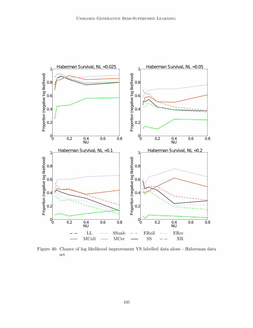
Unbiased Generative Semi-Supervised Learning
0 0.2 0.4 0.6 0.80
0.2
0.4
0.6
0.8
1
NU
Pro
portio
n(n
egative
log
likelih
ood)
Haberman Survival, NL =0.025
0 0.2 0.4 0.6 0.80
0.2
0.4
0.6
0.8
1
NU
Pro
portio
n(n
egative
log
likelih
ood)
Haberman Survival, NL =0.05
0 0.2 0.4 0.6 0.80
0.2
0.4
0.6
0.8
1
NU
Pro
portio
n(n
egative
log
likelih
ood)
Haberman Survival, NL =0.1
0 0.2 0.4 0.6 0.80
0.2
0.4
0.6
0.8
1
NU
Pro
portio
n(n
egative
log
likelih
ood)
Haberman Survival, NL =0.2
LL SSunb ERnll ERerMCnll MCer SS XR
Figure 46: Chance of log likelihood improvement VS labelled data alone - Haberman dataset
435

Fox-Roberts and Rosten
0 0.2 0.4 0.6 0.80
0.2
0.4
0.6
0.8
1
NU
Proportion(error)
Pima IndianDiabetes, NL =0.025
0 0.2 0.4 0.6 0.80
0.2
0.4
0.6
0.8
1
NU
Proportion(error)
Pima IndianDiabetes, NL =0.05
0 0.2 0.4 0.6 0.80
0.2
0.4
0.6
0.8
1
NU
Proportion(error)
Pima IndianDiabetes, NL =0.1
0 0.2 0.4 0.6 0.80
0.2
0.4
0.6
0.8
1
NU
Proportion(error)
Pima IndianDiabetes, NL =0.2
LL SSunb ERnll ERerMCnll MCer SS XR
Figure 47: Chance of error rate improvement VS labelled data alone - Pima Indian dataset
436

Unbiased Generative Semi-Supervised Learning
0 0.2 0.4 0.6 0.80
0.2
0.4
0.6
0.8
1
NU
Pro
portio
n(n
egative
log
likelih
ood)
Pima Indian Diabetes, NL =0.025
0 0.2 0.4 0.6 0.80
0.2
0.4
0.6
0.8
1
NU
Pro
portio
n(n
egative
log
likelih
ood)
Pima Indian Diabetes, NL =0.05
0 0.2 0.4 0.6 0.80
0.2
0.4
0.6
0.8
1
NU
Pro
portio
n(n
egative
log
likelih
ood)
Pima Indian Diabetes, NL =0.1
0 0.2 0.4 0.6 0.80
0.2
0.4
0.6
0.8
1
NU
Pro
portio
n(n
egative
log
likelih
ood)
Pima Indian Diabetes, NL =0.2
LL SSunb ERnll ERerMCnll MCer SS XR
Figure 48: Chance of log likelihood improvement VS labelled data alone - Pima Indian dataset
437

Fox-Roberts and Rosten
0 0.2 0.4 0.6 0.80
0.2
0.4
0.6
0.8
1
NU
Proportion(error)
Fourclass, NL =0.025
0 0.2 0.4 0.6 0.80
0.2
0.4
0.6
0.8
1
NU
Proportion(error)
Fourclass, NL =0.05
0 0.2 0.4 0.6 0.80
0.2
0.4
0.6
0.8
1
NU
Proportion(error)
Fourclass, NL =0.1
0 0.2 0.4 0.6 0.80
0.2
0.4
0.6
0.8
1
NU
Proportion(error)
Fourclass, NL =0.2
LL SSunb ERnll ERerMCnll MCer SS XR
Figure 49: Chance of error rate improvement VS labelled data alone - Fourclass data set
438

Unbiased Generative Semi-Supervised Learning
0 0.2 0.4 0.6 0.80
0.2
0.4
0.6
0.8
1
NU
Proportion(negativeloglikelihood)
Fourclass, NL =0.025
0 0.2 0.4 0.6 0.80
0.2
0.4
0.6
0.8
1
NU
Proportion(negativeloglikelihood)
Fourclass, NL =0.05
0 0.2 0.4 0.6 0.80
0.2
0.4
0.6
0.8
1
NU
Proportion(negativeloglikelihood)
Fourclass, NL =0.1
0 0.2 0.4 0.6 0.80
0.2
0.4
0.6
0.8
1
NU
Proportion(negativeloglikelihood)
Fourclass, NL =0.2
LL SSunb ERnll ERerMCnll MCer SS XR
Figure 50: Chance of log likelihood improvement VS labelled data alone - Fourclass dataset
439

Fox-Roberts and Rosten
References
M. Balcan and A. Blum. An augmented PAC model for semi-supervised learning. In OliverChapelle, B. Scholkopf, and A. Zien, editors, Semi-Supervised Learning, pages 383–404.MIT Press, 2005.
C. Beecks, A. Ivanescu, S. Kirchhoff, and T. Seidl. Modeling image similarity by gaussianmixture models and the signature quadratic form distance. In Computer Vision (ICCV),2011 IEEE International Conference On, pages 1754–1761, 2011.
C. Bishop. Pattern Recognition And Machine Learning. Springer, 2006.
A. Blum and N. Balcan. A discriminative model for semi-supervised learning. In JournalOf The ACM (JACM), volume 57, pages 19:1–19:46, 2010.
A. Blum and T. Mitchell. Combining labeled and unlabeled data with co-training. InProceedings Of The Workshop On Computational Learning Theory, pages 92–100, 1998.
V. Castelli and T. Cover. On the exponential value of labeled samples. Pattern RecognitionLetters, 16(1):105 – 111, 1995.
V. Castelli and T. Cover. The relative value of labeled and unlabeled samples in patternrecognition with an unknown mixing parameter. Information Theory, IEEE Transactionson, 42(6):2102 – 2117, 1996.
F. Cozman and I. Cohen. Unlabeled data can degrade classification performance of gener-ative classifiers. In Fifteenth International Florida Artificial Intelligence Society Confer-ence, pages 327–331, 2002.
F. Cozman and I. Cohen. Risks of semi-supervised learning: How unlabelled data candegrade performance of generative classifiers. In O. Chapelle, B. Scholkopf, and A. Zien,editors, Semi-Supervised Learning, pages 57–72. MIT press, 2006.
F. Cozman, I. Cohen, M. Cirelo, and E. Politecnica. Semi-supervised learning of mixturemodels. In Proceedings Of The 20th International Conference On Machine Learning(ICML), pages 99–106, 2003.
J. Dillon, K. Balasubramanian, and G. Lebanon. Asymptotic analysis of generative semi-supervised learning. In Proceedings Of The 27th International Conference On MachineLearning (ICML), 2010.
G. Druck, C. Pal, A. McCallum, and X. Zhu. Semi-supervised classification with hybridgenerative/discriminative methods. In KDD ’07: Proceedings Of The 13th ACM SIGKDDInternational Conference On Knowledge Discovery And Data Mining, pages 280–289,2007.
A. Frank and A. Asuncion. UCI machine learning repository, 2010. URL http://archive.
ics.uci.edu/ml.
Y. Grandvalet and Y. Bengio. Entropy Regularization. In Semi-Supervised Learning, pages151–168. MIT Press, 2006.
440

Unbiased Generative Semi-Supervised Learning
T. Ho and E. Kleinberg. Building projectable classifiers of arbitrary complexity. In Inter-national Conference On Pattern Recognition (ICPR), volume 2, pages 880–885, 1996.
C. Hsu, C. Chang, and C. Lin. A practical guide to support vector classification. Technicalreport, Department of Computer Science, National Taiwan University, 2003.
G. Hughes. On the mean accuracy of statistical pattern recognizers. Information Theory,IEEE Transactions On, 14(1):55 – 63, 1968.
T. Jaakkola and D. Haussler. Exploiting generative models in discriminative classifiers.In Proceedings Of The 1998 Conference On Advances In Neural Information ProcessingSystems II, pages 487–493, 1999.
E. Jaynes. Probability Theory. Cambridge University Press, 2003.
H. Kang, S. Yoo, and D. Han. Senti-lexicon and improved naıve bayes algorithms forsentiment analysis of restaurant reviews. Expert Systems With Applications, 39(5):6000– 6010, 2012.
B. Krishnapuram, D. Williams, Y. Xue, A. Hartemink, L. Carin, and M. Figueiredo. Onsemi-supervised classification. In Advances In Neural Information Processing Systems(NIPS), pages 721–728, 2005.
J. Lagarias, J. Reeds, M. Wright, and P. Wright. Convergence properties of the Nelder-Mead simplex method in low dimensions. SIAM Journal Of Optimization, 9(1):112–147,1998.
J. Lasserre, C. Bishop, and T. Minka. Principled hybrids of generative and discriminativemodels. In Computer Vision And Pattern Recognition (CVPR), volume 1, pages 87 – 94,2006.
J. Lucke and J. Eggert. Expectation truncation and the benefits of preselection in traininggenerative models. In Journal Of Machine Learning Research (JMLR), pages 2855–2900,October 2010.
D. MacKay. Information Theory, Inference, And Learning Algorithms. Cambridge Univer-sity Press, 2003.
G. Mann and A. McCallum. Simple, robust, scalable semi-supervised learning via Expec-tation Regularization. In Proceedings Of The 24th International Conference On MachineLearning (ICML), pages 593–600, 2007.
A. McCallum, C. Pal, G. Druck, and X. Wang. Multi-conditional learning: Genera-tive/discriminative training for clustering and classification. In National Conference OnArtificial Intelligence, pages 433–439, 2006.
A. Ng and M. Jordan. On discriminative vs. generative classifiers: A comparison of logisticregression and Naive Bayes. Advances In Neural Information Processing Systems (NIPS),2:841–848, 2002.
441

Fox-Roberts and Rosten
K. Nigam, A. McCallum, S. Thrun, and T. Mitchell. Text classification from labeled andunlabeled documents using EM. Machine Learning, 39:103–134, 2000.
J. Nocedal and S. Wright. Numerical Optimization, Springer Series In Operations Research.Springer-Verlag, 1999.
J. Ratsaby and S. Venkatesh. Learning from a mixture of labeled and unlabeled exampleswith parametric side information. In Conference On Learning Theory (COLT), pages412–417, 1995.
I. Rauschert and R. Collins. A generative model for simultaneous estimation of human bodyshape and pixel-level segmentation. In Proceedings Of The 12th European Conference OnComputer Vision - Volume Part V, European Conference On Computer Vision (ECCV),pages 704–717. Springer-Verlag, 2012.
S. Rosset, J. Zhu, H. Zou, and T. Hastie. A method for inferring label sampling mecha-nisms in semi-supervised learning. In Advances In Neural Information Processing Systems(NIPS), volume 17, pages 1161 – 1168, 2005.
B. Shahshahani and D. Landgrebe. The effect of unlabeled samples in reducing the smallsample size problem and mitigating the Hughes phenomenon. Geoscience And RemoteSensing, IEEE Transactions on, 32(5):1087 –1095, 1994.
A. Subramanya and J. Bilmes. Soft-supervised learning for text classification. In ProceedingsOf The Conference On Empirical Methods In Natural Language Processing, pages 1090–1099, 2008.
A. Subramanya and J. Bilmes. Entropic graph regularization in non-parametric semi-supervised classification. In Advances In Neural Information Processing Systems (NIPS),December 2009.
U. Syed and B. Taskar. Semi-supervised learning with adversarially missing label informa-tion. In Advances In Neural Information Processing Systems (NIPS), pages 2244–2252,2010.
M. Szummer and T. Jaakkola. Information Regularization with partially labeled data. InAdvances In Neural Information Processing Systems (NIPS), 2002.
V. Vapnik. Statistical Learning Theory. John Wiley & Sons, Inc, 1998.
J. Wang, X. Shen, and W. Pan. On transductive support vector machines. In PredictionAnd Discovery. American Mathematical Society, 2007.
T. Yang and C. Priebe. The effect of model misspecification on semi-supervised classifica-tion. Pattern Analysis And Machine Intelligence (PAMI), 33:2093–2103, 2011.
I. Yeh, K. Yang, and T. Ting. Knowledge discovery on RFM model using Bernoulli sequence.Expert Systems With Applications, 36(3, Part 2):5866 – 5871, 2009.
T. Zhang. The value of unlabeled data for classification problems. In International Con-ference On Machine Learning (ICML), pages 1191–1198, 2000.
442

Unbiased Generative Semi-Supervised Learning
X. Zhu. Semi-supervised learning literature survey. Technical report, Department of Com-puter Sciences, University of Wisconsin, Madison, 2005.
F. Zhuang, P. Luo, Z. Shen, Q. He, Y. Xiong, Z. Shi, and H. Xiong. Mining distinctionand commonality across multiple domains using generative model for text classification.Knowledge And Data Engineering, IEEE Transactions On, 24(11):2025–2039, 2012.
443
Related Documents