UCLA Electronic Theses and Dissertations - eScholarship.org

UCLAUCLA Electronic Theses and Dissertations

TitleMultiscale and Patient-Specific Cardiovascular Modeling

Permalinkhttps://escholarship.org/uc/item/4431d048

AuthorCanuto, Daniel Joseph

Publication Date2019 Peer reviewed|Thesis/dissertation

eScholarship.org Powered by the California Digital LibraryUniversity of California

https://escholarship.org/uc/item/4431d048

https://escholarship.org

http://www.cdlib.org/

UNIVERSITY OF CALIFORNIA

Los Angeles

Multiscale and Patient-Specific Cardiovascular Modeling

A dissertation submitted in partial satisfaction

of the requirements for the degree

Doctor of Philosophy in Mechanical Engineering

by

Daniel Canuto

2019

c© Copyright by

Daniel Canuto

2019

ABSTRACT OF THE DISSERTATION

Multiscale and Patient-Specific Cardiovascular Modeling

by

Daniel Canuto

Doctor of Philosophy in Mechanical Engineering

University of California, Los Angeles, 2019

Professor Jeffrey D. Eldredge, Chair

Despite continuing advances in computational power, full-body models of the human car-

diovascular system remain a costly task. Two principal reasons for this cost are the total

overall length of the vascular network (spanning O(108) m) and the broad range of length

scales (from 10−2 to 10−6 m) involved. Multiscale modeling can be employed to overcome

these issues; specifically, subsystems of higher spatial dimension representing domains of

interest can be coupled at their boundaries to lower-dimensional subsystems that mimic

relevant inflow/outflow conditions. Though this scheme can increase computational effi-

ciency, the inherent reduction in spatial dimension results in parameterizations that can

be difficult to optimize in patient-specific contexts. This work is divided into two parts:

in the first segment, a closed-loop multiscale model of the entire cardiovascular system is

developed and integrated with a feedback control model for blood pressure regulation. It

is tested against clinical data for cohorts of healthy subjects, and its predictive utility is

demonstrated in a simulation of acute hemorrhage from the upper leg. After validating the

multiscale/reduced-order approach, a parameter optimization technique based on the ensem-

ble Kalman filter (EnKF) is constructed. By assimilating patients’ clinical measurements,

this method is shown to successfully tune parameters in two models: a zero-dimensional

model of the pulmonary circulation, and a multiscale 0D-1D model of the lower leg.

ii

The dissertation of Daniel Canuto is approved.

Kunihiko Taira

Xiaolin Zhong

Joseph M. Teran

Jeffrey D. Eldredge, Committee Chair

University of California, Los Angeles

2019

iii

TABLE OF CONTENTS

1 Introduction . . . . . . . . . . . . . . . . . . . . . . . . . . . . . . . . . . . . . . 1

1.1 Background . . . . . . . . . . . . . . . . . . . . . . . . . . . . . . . . . . . . 1

1.1.1 The cardiovascular system . . . . . . . . . . . . . . . . . . . . . . . . 1

1.1.2 Cardiovascular control . . . . . . . . . . . . . . . . . . . . . . . . . . 7

1.2 Previous modeling efforts . . . . . . . . . . . . . . . . . . . . . . . . . . . . . 10

1.2.1 Zero-dimensional (lumped parameter) modeling . . . . . . . . . . . . 10

1.2.2 Higher-dimensional and multiscale modeling . . . . . . . . . . . . . . 12

1.2.3 Regulatory control modeling . . . . . . . . . . . . . . . . . . . . . . . 13

1.3 Objectives . . . . . . . . . . . . . . . . . . . . . . . . . . . . . . . . . . . . . 15

2 Construction of a Full-Scale Cardiovascular Model . . . . . . . . . . . . . 17

2.1 Systemic arterial submodel . . . . . . . . . . . . . . . . . . . . . . . . . . . . 17

2.1.1 Basic model of a single artery . . . . . . . . . . . . . . . . . . . . . . 17

2.1.2 Arterial numerical solution . . . . . . . . . . . . . . . . . . . . . . . . 23

2.2 Cardiac submodel . . . . . . . . . . . . . . . . . . . . . . . . . . . . . . . . . 26

2.3 Pulmonary submodel . . . . . . . . . . . . . . . . . . . . . . . . . . . . . . . 29

2.4 Peripheral submodel . . . . . . . . . . . . . . . . . . . . . . . . . . . . . . . 30

2.5 0D-1D coupling . . . . . . . . . . . . . . . . . . . . . . . . . . . . . . . . . . 31

2.5.1 Proximal coupling . . . . . . . . . . . . . . . . . . . . . . . . . . . . . 31

2.5.2 Distal coupling . . . . . . . . . . . . . . . . . . . . . . . . . . . . . . 33

2.6 Baroreflex submodel . . . . . . . . . . . . . . . . . . . . . . . . . . . . . . . 33

2.7 Tabulated parameter values by submodel . . . . . . . . . . . . . . . . . . . . 36

3 Full-Scale Model Results and Analysis . . . . . . . . . . . . . . . . . . . . . 45

iv

3.1 Validation under resting conditions . . . . . . . . . . . . . . . . . . . . . . . 45

3.2 Response to global sympathetic stimulation . . . . . . . . . . . . . . . . . . 48

3.3 Response to 10% acute hemorrhage . . . . . . . . . . . . . . . . . . . . . . . 54

3.4 Parameter Sensitivity Analysis . . . . . . . . . . . . . . . . . . . . . . . . . . 58

3.4.1 The Latin-Hypercube/one-at-a-time method . . . . . . . . . . . . . . 58

3.4.2 LH-OAT analysis of the full-scale cardiovascular model . . . . . . . . 60

4 Data Assimilation and Parameter Estimation . . . . . . . . . . . . . . . . . 67

4.1 Overview of the Kalman filter framework . . . . . . . . . . . . . . . . . . . . 67

4.2 The classical Kalman filter . . . . . . . . . . . . . . . . . . . . . . . . . . . . 70

4.3 The ensemble Kalman filter (EnKF) . . . . . . . . . . . . . . . . . . . . . . 72

4.3.1 Evensen’s original method . . . . . . . . . . . . . . . . . . . . . . . . 72

4.3.2 Covariance inflation . . . . . . . . . . . . . . . . . . . . . . . . . . . . 73

4.4 EnKF parameter estimation methods . . . . . . . . . . . . . . . . . . . . . . 75

4.4.1 Joint versus dual estimation . . . . . . . . . . . . . . . . . . . . . . . 75

4.4.2 The complete parameter estimation procedure . . . . . . . . . . . . . 76

4.5 A simple EnKF example implementation . . . . . . . . . . . . . . . . . . . . 77

4.5.1 Model formulation . . . . . . . . . . . . . . . . . . . . . . . . . . . . 77

4.5.2 Results . . . . . . . . . . . . . . . . . . . . . . . . . . . . . . . . . . . 80

5 EnKF Estimation of Submodel Parameters . . . . . . . . . . . . . . . . . . 83

5.1 EnKF implementation for a 0D cardiovascular model . . . . . . . . . . . . . 83


5.1.2 Results . . . . . . . . . . . . . . . . . . . . . . . . . . . . . . . . . . . 85

5.2 EnKF implementation for a coupled 0D-1D cardiovascular model . . . . . . . 89


v

5.2.2 Results . . . . . . . . . . . . . . . . . . . . . . . . . . . . . . . . . . . 95

5.3 Tables of parameter values, distribution characteristics, and model geometry 98

6 Conclusion . . . . . . . . . . . . . . . . . . . . . . . . . . . . . . . . . . . . . . . 104

6.1 Summary and Future Work . . . . . . . . . . . . . . . . . . . . . . . . . . . 104

6.2 Publications and Presentations . . . . . . . . . . . . . . . . . . . . . . . . . 105

References . . . . . . . . . . . . . . . . . . . . . . . . . . . . . . . . . . . . . . . . . 107

vi

LIST OF FIGURES

1.1 Cross-sectional schematic of the human heart [Pie06]. . . . . . . . . . . . . . . . 2

1.2 A Wiggers diagram, illustrating the phases of the cardiac cycle for the left heart

(reproduced from Wikimedia Commons under the GNU Free Documentation Li-

cense). . . . . . . . . . . . . . . . . . . . . . . . . . . . . . . . . . . . . . . . . . 3

1.3 Comparison of blood vessel structure for (a) arteries and (b) veins [TD09]. . . . 5

1.4 Summary of the input-output profile of the cardiovascular center [TD09]. . . . . 7

1.5 Frank’s [Fra99] two-element Windkessel (diagram from [Ker17]). . . . . . . . . . 11

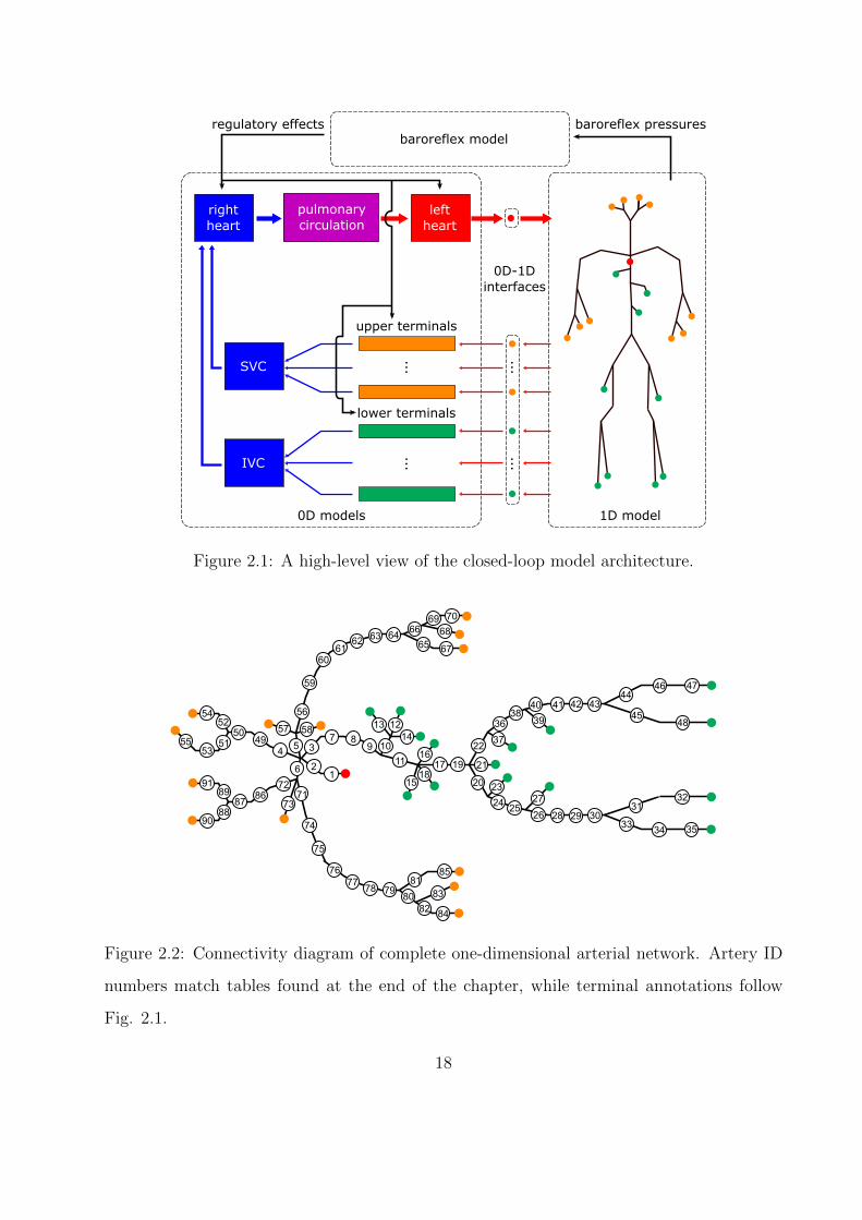
2.1 A high-level view of the closed-loop model architecture. . . . . . . . . . . . . . . 18

2.2 Connectivity diagram of complete one-dimensional arterial network. Artery ID

numbers match tables found at the end of the chapter, while terminal annotations

follow Fig. 2.1. . . . . . . . . . . . . . . . . . . . . . . . . . . . . . . . . . . . . 18

2.3 One-dimensional control volume representation of a single artery (adapted from

[SFP03]). Note the domain boundaries: x ∈ [0, L]. . . . . . . . . . . . . . . . . . 19

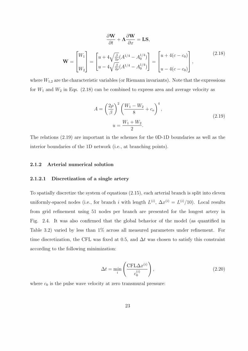
2.4 Selected localized results from a grid refinement study in the one-dimensional

arterial network. . . . . . . . . . . . . . . . . . . . . . . . . . . . . . . . . . . . 24

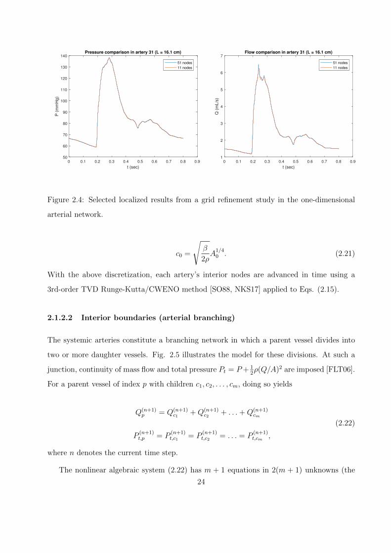
2.5 Schematic of an arterial splitting node. The index i ranges from 1 to m, the

number of children at the split, while the index n denotes the current time step.

In the spatial discretization, the parent’s most distal node coincides with the most

proximal node of each child. . . . . . . . . . . . . . . . . . . . . . . . . . . . . . 25

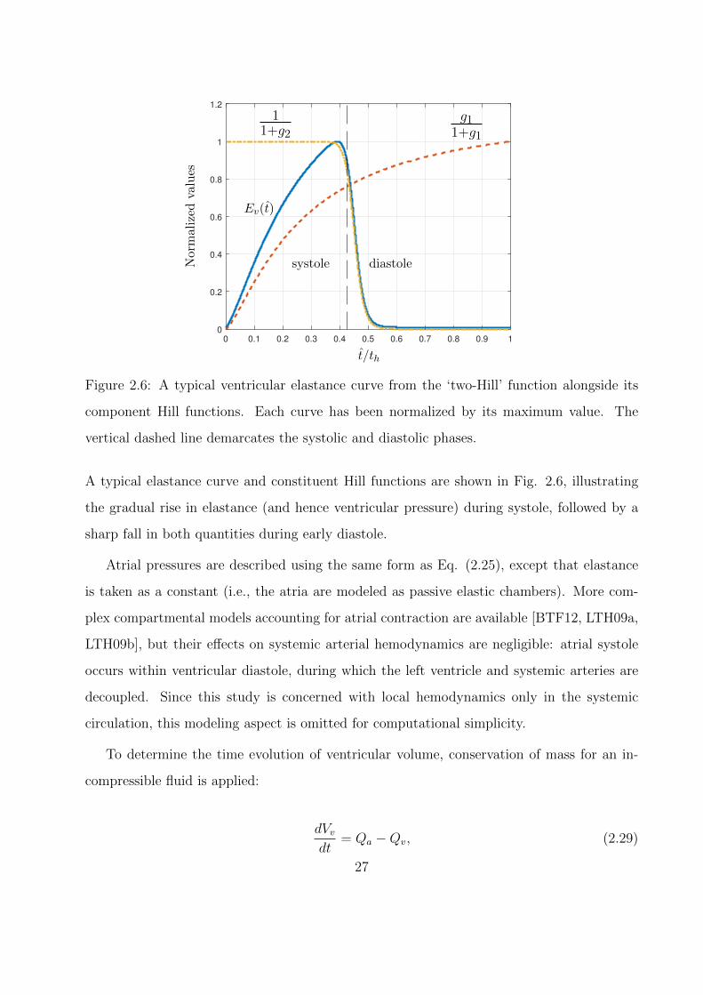
2.6 A typical ventricular elastance curve from the ‘two-Hill’ function alongside its

component Hill functions. Each curve has been normalized by its maximum

value. The vertical dashed line demarcates the systolic and diastolic phases. . . 27

vii

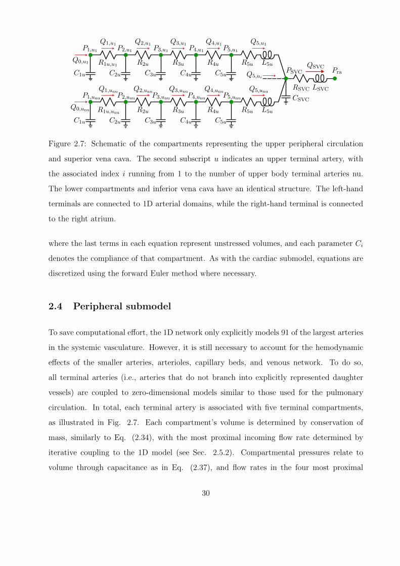
2.7 Schematic of the compartments representing the upper peripheral circulation and

superior vena cava. The second subscript u indicates an upper terminal artery,

with the associated index i running from 1 to the number of upper body terminal

arteries nu. The lower compartments and inferior vena cava have an identical

structure. The left-hand terminals are connected to 1D arterial domains, while

the right-hand terminal is connected to the right atrium. . . . . . . . . . . . . . 30

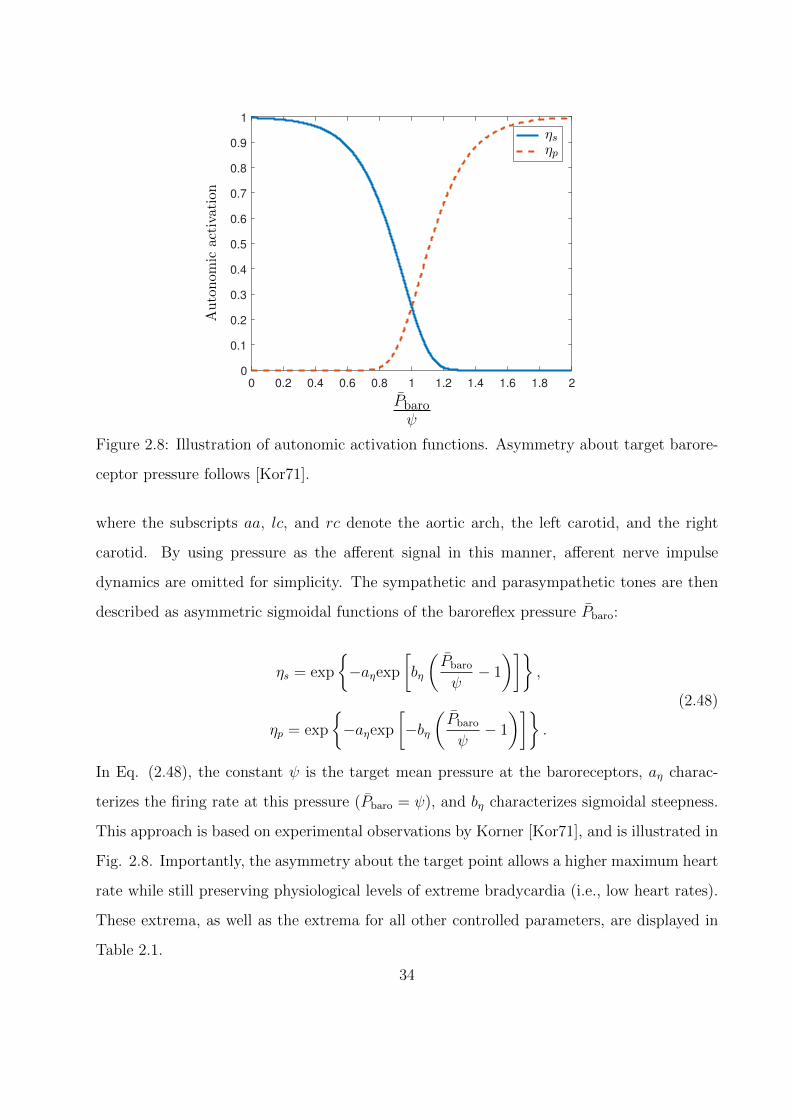
2.8 Illustration of autonomic activation functions. Asymmetry about target barore-

ceptor pressure follows [Kor71]. . . . . . . . . . . . . . . . . . . . . . . . . . . . 34

3.1 Spatio-temporal evolution of the pressure waveform traveling from the aortic root

(D = 0 cm) to the left anteriortibial artery under resting conditions. . . . . . . . 46

3.2 Flow rate measured under resting conditions at varying distances D from the

aortic root. . . . . . . . . . . . . . . . . . . . . . . . . . . . . . . . . . . . . . . 47

3.3 Global clinical parameters of interest at equilibria achieved under varying levels

of sympathetic stimulation/parasympathetic inhibition. Dashed line represents

limit for non-emergency hypertension (systolic BP ≤ 179 mmHg, diastolic BP

≤ 109 mmHg). . . . . . . . . . . . . . . . . . . . . . . . . . . . . . . . . . . . . 51

3.4 Pressure measured across the 1D network at varying levels of sympathetic stim-

ulation/parasympathetic inhibition (note ns = 0.25 is the baseline case). . . . . 53

3.5 Sympathetic activation, baroreceptor pressure, and effector organ responses dur-

ing acute 10% hemorrhage. Pressure and effector responses (excluding heart

rate) normalized by basal values. Region between dashed lines indicates period

of tourniquet application. . . . . . . . . . . . . . . . . . . . . . . . . . . . . . . 55

3.6 Shift in blood distribution during an acute 10% hemorrhage. Volumes normalized

by volume at end-diastole just before hemorrhage (i.e., the healthy condition).

Region between dashed lines indicates period of tourniquet application. . . . . . 57

viii

3.7 Comparison of aortic pressure and equilibrium cardiac pressure-volume loops with

and without intact baroreflex during 10% hemorrhage. Region between dashed

lines indicates period of tourniquet application. . . . . . . . . . . . . . . . . . . 58

3.8 Example of valid Latin Hypercube sampling regions (in blue) for a 2D parameter

space. . . . . . . . . . . . . . . . . . . . . . . . . . . . . . . . . . . . . . . . . . 60

3.9 Normalized LH-OAT parameter sensitivities for various clinical measurement pre-

dictions. Scaling indices are linked to parameters tabulated in Table 3.5. . . . . 66

4.1 Schematic of a resistive flow splitter used for EnKF demonstration. Note that

both outlets are connected to ground pressure. . . . . . . . . . . . . . . . . . . . 78

4.2 Comparison of ensemble mean predictions for varying levels of measurement avail-

ability. Note that all quantities are dimensionless. . . . . . . . . . . . . . . . . . 81

5.1 Schematic of the compartmental cardiovascular model used for EnKF testing. . 83

5.2 Evolution of selected parameter variances (normalized by initial ensemble mean

values) during optimization for the 0D pulmonary model. . . . . . . . . . . . . . 87

5.3 Converged ensemble flow rate comparison against patient MRI data during sys-

tole. Shaded blue area is the middle 95% quantile of the ensembles. . . . . . . . 88

5.4 Comparison of pressure-volume traces during systole for the converged healthy

and hypertensive cases. EF: ejection fraction. . . . . . . . . . . . . . . . . . . . 88

5.5 Input impedance and ventricular elastance comparisons for healthy and hyper-

tensive cases. . . . . . . . . . . . . . . . . . . . . . . . . . . . . . . . . . . . . . 89

5.6 Connectivity diagram of complete one-dimensional arterial network. Inset shows

a representative 0D terminal outlet, present at all green nodes. The red node is

the inflow boundary, while blue nodes represent velocity measurement locations

for the EnKF parameter estimator. Artery ID numbers match Table 5.5. . . . . 91

ix

5.7 Converged ensemble velocity prediction compared against patient measurements

for the coupled 0D-1D lower leg case. Shaded blue region is the middle 95%

quantile. . . . . . . . . . . . . . . . . . . . . . . . . . . . . . . . . . . . . . . . . 96

5.8 Ensemble mean pressure traces at inflow (popliteal) and outflow (all other) ar-

teries for the coupled 0D-1D lower leg case. . . . . . . . . . . . . . . . . . . . . 97

5.9 Evolution of selected parameter variances (normalized by initial ensemble mean

values) during optimization for the coupled 0D-1D lower leg model. . . . . . . . 98

x

LIST OF TABLES

2.1 Ranges of baroreflex-controlled parameters, normalized by parameter values at

basal autonomic activation. . . . . . . . . . . . . . . . . . . . . . . . . . . . . . 35

2.2 Time constants for autonomic effector organs. . . . . . . . . . . . . . . . . . . . 36

2.3 Parameters for the one-dimensional arterial network. . . . . . . . . . . . . . . . 37

2.4 Parameters for the cardiac/pulmonary submodel. Note that Elv,max and Erv,max

are nominal values subject to change in the event of autoregulation. . . . . . . . 40

2.5 Parameters for 0D terminal compartments and vena cavae. Unless otherwise

noted, upper and lower terminal compartments share values. . . . . . . . . . . . 41

2.6 Parameters for liver compartments. . . . . . . . . . . . . . . . . . . . . . . . . . 42

2.7 Parameters for baroreflex submodel. . . . . . . . . . . . . . . . . . . . . . . . . 43

3.1 Comparison of predicted regional blood flow with experimental data. . . . . . . 46

3.2 Clinical parameters of interest under resting conditions with empirically-measured

ranges. SBP: systolic blood pressure; DBP: diastolic blood pressure; LV/RV

EDV/RSV: left/right ventricular end-diastolic/end-systolic volume; LV/RV EF:

left/right ventricular ejection fraction; HR: heart rate; CO: cardiac output; SVR:

systemic vascular resistance; PWV: pulse wave velocity. *PWV estimated by

following the foot of the pressure pulse from the aortic inlet to the outlet of the

left posterior tibial artery. . . . . . . . . . . . . . . . . . . . . . . . . . . . . . . 49

3.3 Comparison of global clinical parameters under sympathetic stimulation/parasympathetic

inhibition against literature data from patients with pheochromocytoma (matched

by mean arterial pressure at 134 mmHg). . . . . . . . . . . . . . . . . . . . . . . 52

3.4 Percentage changes (relative to healthy value) during hemorrhage compared against

numerical [BTF12] and experimental [FRH11, KSS70] data from the literature. . 59

3.5 Listing of parameter scalings associated with indices in Fig. 3.9. . . . . . . . . . 61

xi

4.1 Normal distribution characteristics for flow splitter resistances. . . . . . . . . . . 80

4.2 L2 norm of error for ensemble mean predictions across varying levels of measure-

ment availability. . . . . . . . . . . . . . . . . . . . . . . . . . . . . . . . . . . . 81

5.1 Time-averaged velocity comparisons between model predictions and clinicial data

for the coupled 0D-1D lower leg case. . . . . . . . . . . . . . . . . . . . . . . . . 97

5.2 Normal distribution characteristics for 0D pulmonary model parameters. . . . . 98

5.3 Converged parameter values for the 0D model in the healthy case. . . . . . . . . 99

5.4 Converged parameter values for the 0D model in the hypertensive case. . . . . . 99

5.5 Geometric data for the one-dimensional arterial network. . . . . . . . . . . . . . 100

5.6 Normal distribution characteristics for coupled 0D-1D lower leg model parameters.101

5.7 Converged ensemble mean parameter values for the coupled 0D-1D lower leg model.101

xii

ACKNOWLEDGMENTS

I’m pretty exhausted, so I’m sure this list won’t be exhaustive, but here goes. To Mom, for

always telling me I would do great things. To Dad, for exhorting me to be a leader, not a

follower. To Stephen, for being my jelly preserver since the day I was born. To Julie, for

telling me that I’m amazing on days when I feel quite the opposite. To all my friends back

east, for keeping me humble and sane. To Sam, for introducing a bewildered undergrad to

the weird, wonderful world of research. And finally, to Jeff, for asking the right questions

and nudging me in the right directions. This work would never have been possible without

y’all’s advice and encouragement, and I am deeply grateful.

xiii

CHAPTER 1

Introduction

1.1 Background

In terms of its fluid dynamics, the human cardiovascular system is immensely complex. The

flow is pulsatile, transitions between laminar and turbulent [Ku97], involves fluid-structure

interactions [TOK06], and has characteristic length scales spanning several orders of mag-

nitude [TD09]. The relevant anatomy is no simpler: the heart is a four-chambered, electro-

chemical pump [TD09], delivering blood to a network of vessels whose total length is O(108)

meters [LE04]. Moreover, both the heart and the vasculature can be regulated by local

[LCG03] and global [Kor71] control, incorporating sensors for pressure [Dan98], blood vol-

ume [AHM76], lung inflation [AT84], and chemical concentration [Dam94]. As such, a com-

plete description of the cardiovascular system is well beyond the scope of the present work.

Instead, this chapter outlines only the anatomical and physiological features whose modeling

is attempted, followed by a brief history of relevant modeling work from the literature. With

this context in mind, the chapter closes with the objectives of this work.

1.1.1 The cardiovascular system

1.1.1.1 Heart

The heart is the cornerstone of the cardiovascular system, its contractions creating the

pressure difference required to transport blood through the body. Fig. 1.1 shows a cross-

sectional schematic of the heart and its major connections [Pie06]. The ventricles’ primary

function is to send blood from the heart: the right ventricle pumps deoxygenated blood

1

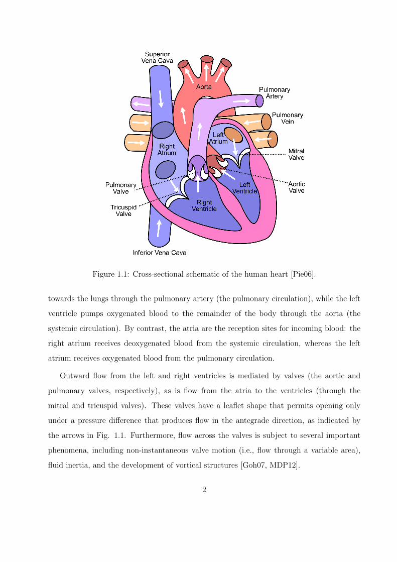
Figure 1.1: Cross-sectional schematic of the human heart [Pie06].

towards the lungs through the pulmonary artery (the pulmonary circulation), while the left

ventricle pumps oxygenated blood to the remainder of the body through the aorta (the

systemic circulation). By contrast, the atria are the reception sites for incoming blood: the

right atrium receives deoxygenated blood from the systemic circulation, whereas the left

atrium receives oxygenated blood from the pulmonary circulation.

Outward flow from the left and right ventricles is mediated by valves (the aortic and

pulmonary valves, respectively), as is flow from the atria to the ventricles (through the

mitral and tricuspid valves). These valves have a leaflet shape that permits opening only

under a pressure difference that produces flow in the antegrade direction, as indicated by

the arrows in Fig. 1.1. Furthermore, flow across the valves is subject to several important

phenomena, including non-instantaneous valve motion (i.e., flow through a variable area),

fluid inertia, and the development of vortical structures [Goh07, MDP12].

2

Isov

olum

ic con

traction

Ejection

Isov

olum

ic re

laxa

tion

Rap

id in

flow

Diastas

is

Atri

al sys

tole

Aortic pressure

Atrial pressure

Ventricular pressure

Ventricular volume

Electrocardiogram

Phonocardiogram

Systole Diastole Systole

1st 2nd 3rd

P

R

T

QS

a c vPre

ssu

re (

mm

Hg)

120

100

80

60

40

20

0

Vo

lum

e (

mL) 130

90

50

Aortic valve

opens

Aortic valve

closes

Mitral valve

closes

Mitral valve

opens

Figure 1.2: A Wiggers diagram, illustrating the phases of the cardiac cycle for the left heart

(reproduced from Wikimedia Commons under the GNU Free Documentation License).

3

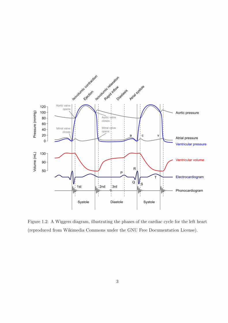
The opening and closing of the cardiac valves, and hence the flow of blood through the

body, happens as a consequence of the rhythmic contraction and relaxation of the heart’s

muscular tissue (the myocardium). This process is the cardiac cycle, and is commonly

visualized by a collection of plots known as the “Wiggers diagram,” as reproduced in Fig. 1.2.

Referring to the diagram, the first portion of the cycle is called systole, and is characterized by

flow from the ventricles into the vasculature. In early systole, the ventricular myocardium

recieves an electrical signal and depolarizes (the so-called “QRS complex” labeled on the

electrocardiogram), causing a muscular contraction that rapidly raises the pressure of the

blood within the ventricle. Once ventricular pressure exceeds aortic pressure, the aortic

valve opens, allowing blood to eject into the aorta and be distributed through the systemic

circulation.

As the ventricle empties and relaxes, its internal pressure falls, eventually dropping below

aortic pressure and leading to the closure of the aortic valve. At the same time, the ventricle

electrically repolarizes to prepare for the next cycle, as shown by the “T wave” on the

electrocardiogram. As this repolarization ends, the heart begins its diastolic phase, in whcih

the ventricles are refilled for the next cycle. This phase begins with a short period of

ventricular relaxation at constant volume, as both the aortic and mitral valves are closed.

Upon complete ventricular relaxation, atrial pressure exceeds ventricular pressure, leading

to the opening of the mitral valve and an initially rapid refilling of the ventricle. However,

as the ventricle fills, its pressure rises, leading to a reduction in its filling rate known as

diastasis. To achieve complete refilling, the atrium depolarizes and contracts, resulting in

the “P wave” on the electrocardiogram, the return of the ventricle to its initial volume, and

the completion of the cycle. As a closing remark, note that despite this discussion’s focus on

the left heart, the right heart undergoes a qualitatively identical cycle at a lower pressure:

normal mean pulmonary artery pressure is less than 20 mmHg in healthy adults [DMG87],

whereas a typical value for mean aortic pressure is 83 mmHg [TD09].

4

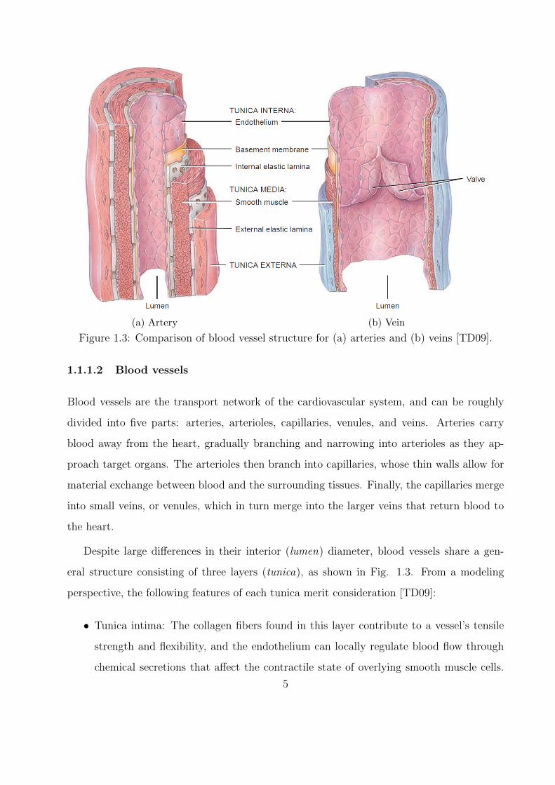
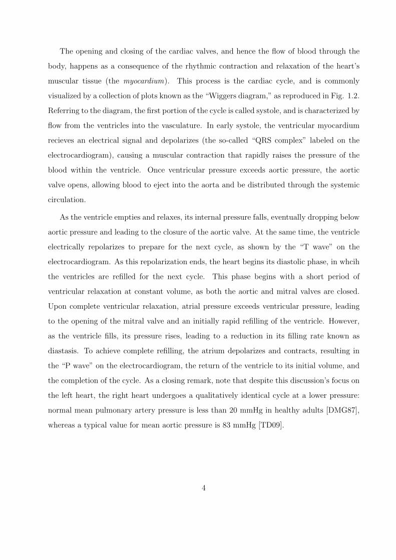
(a) Artery (b) Vein

Figure 1.3: Comparison of blood vessel structure for (a) arteries and (b) veins [TD09].

1.1.1.2 Blood vessels

Blood vessels are the transport network of the cardiovascular system, and can be roughly

divided into five parts: arteries, arterioles, capillaries, venules, and veins. Arteries carry

blood away from the heart, gradually branching and narrowing into arterioles as they ap-

proach target organs. The arterioles then branch into capillaries, whose thin walls allow for

material exchange between blood and the surrounding tissues. Finally, the capillaries merge

into small veins, or venules, which in turn merge into the larger veins that return blood to

the heart.

Despite large differences in their interior (lumen) diameter, blood vessels share a gen-

eral structure consisting of three layers (tunica), as shown in Fig. 1.3. From a modeling

perspective, the following features of each tunica merit consideration [TD09]:

• Tunica intima: The collagen fibers found in this layer contribute to a vessel’s tensile

strength and flexibility, and the endothelium can locally regulate blood flow through

chemical secretions that affect the contractile state of overlying smooth muscle cells.

5

Also, valves composed of endothelial cells in the veins prevent retrograde flow (e.g.,

due to gravity).

• Tunica media: The elastic fibers in this layer allow vessels to flex and recoil in accord

with pressure changes, and the contractile state of its smooth muscle cells are a primary

determinant of lumen diameter.

• Tunica externa: In addition to elastic fibers, this layer also contains nerves that allow

for regulatory action via the central nervous system.

Variations in the specific stucture and relative thicknesses of these three layers (or the ab-

sence of one or more layers) are the source of important functional differences between types

of blood vessels. As sketched in Fig. 1.3, arteries have a much thicker vessel wall compared

to veins of similar overall diameter, principally due to a more extensive tunica media. This

additional smooth muscle allows arteries to withstand the higher pressures found in precap-

illary portions of circulatory routes. On the other hand, capillaries possess only a tunica

intima, and consequently have very thin vessel walls to permit efficient exchange between

blood and external tissues.

Besides differences between arteries, veins, and capillaries, there are also inter-arterial

structural shifts according to size and distance from the heart. In the large arteries nearest

to the heart, the tunica media has a higher concentration of elastic fibers; this property allows

them to first expand and hold blood during systole, then recoil and drive blood towards the

smaller arteries during diastole. For this ability to store and release blood, these arteries

are categorized as “compliance” (or “capacitance”) vessels. In the smaller arteries, and

especially the arterioles, the tunica media is dominated by smooth muscle fibers, meaning

that these vessels can greatly stiffen or relax in response to regulatory stimuli. In the

arterioles, these changes in vascular muscle tone translate to alterations in vessel lumen

diameter, allowing strong mediation of opposition to flow. For this reason, the arterioles are

often called “resistance” vessels. These notions of vascular compliance and resistance are

useful in modeling contexts, as they provide intuitive parameterizations for cardiovascular

elements that are not spatially resolved (see Sec. 1.2.1).

6

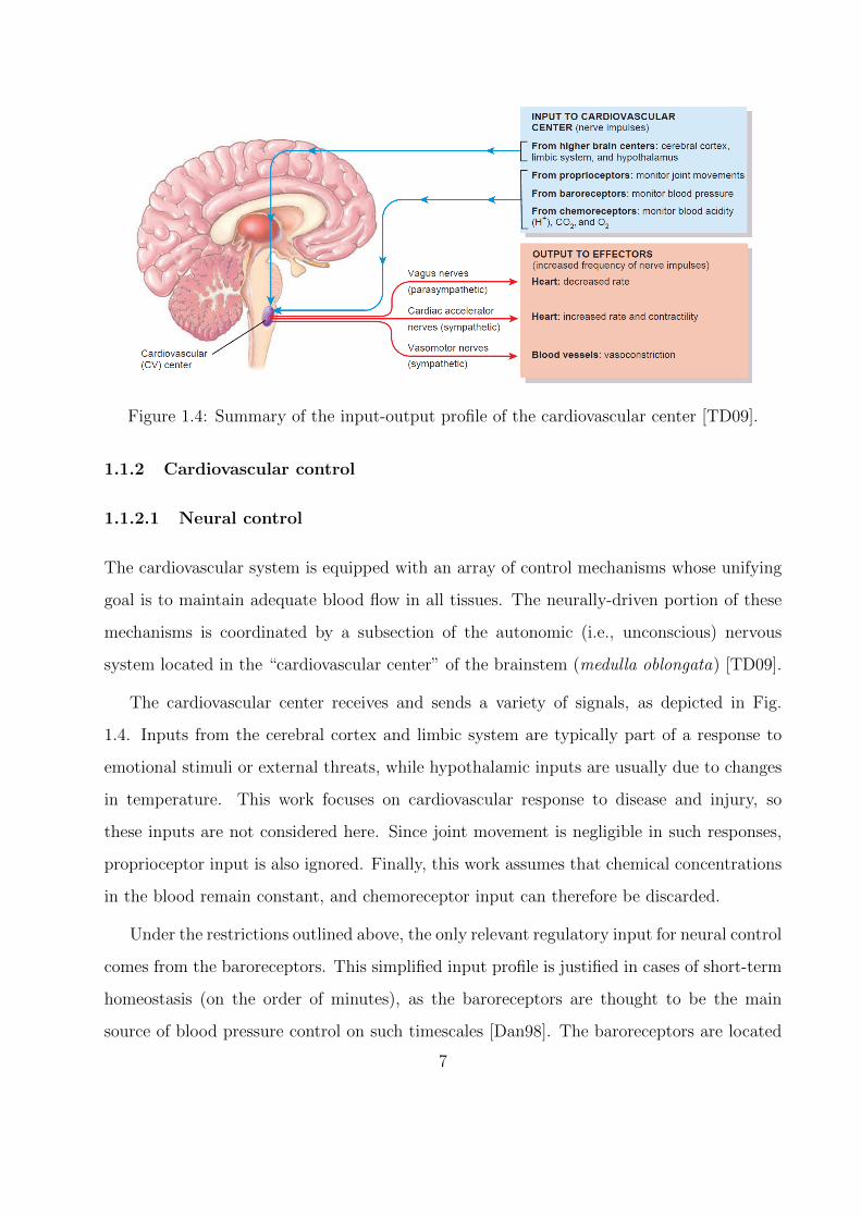
Figure 1.4: Summary of the input-output profile of the cardiovascular center [TD09].

1.1.2 Cardiovascular control

1.1.2.1 Neural control

The cardiovascular system is equipped with an array of control mechanisms whose unifying

goal is to maintain adequate blood flow in all tissues. The neurally-driven portion of these

mechanisms is coordinated by a subsection of the autonomic (i.e., unconscious) nervous

system located in the “cardiovascular center” of the brainstem (medulla oblongata) [TD09].

The cardiovascular center receives and sends a variety of signals, as depicted in Fig.

1.4. Inputs from the cerebral cortex and limbic system are typically part of a response to

emotional stimuli or external threats, while hypothalamic inputs are usually due to changes

in temperature. This work focuses on cardiovascular response to disease and injury, so

these inputs are not considered here. Since joint movement is negligible in such responses,

proprioceptor input is also ignored. Finally, this work assumes that chemical concentrations

in the blood remain constant, and chemoreceptor input can therefore be discarded.

Under the restrictions outlined above, the only relevant regulatory input for neural control

comes from the baroreceptors. This simplified input profile is justified in cases of short-term

homeostasis (on the order of minutes), as the baroreceptors are thought to be the main

source of blood pressure control on such timescales [Dan98]. The baroreceptors are located

7

on both the aortic arch downstream of the aortic valve and on the carotid sinuses, which

are small widenings of the internal carotid arteries leading into the brain. Functionally, they

are mechanical-electrical pressure transducers: blood pressure first causes them to stretch in

tandem with the vessel wall, followed by a conversion of this deformation into a firing rate

of the neurons connected to the receptor sites. This firing rate is the first part of a negative

feedback loop known as the “baroreflex”: if the firing rate deviates from a homeostatic value,

the cardiovascular center sends out signals to the heart and blood vessels (the “effector”

organs in Fig. 1.4) to restore normal blood pressure.

As shown in Fig. 1.4, the cardiovascular center sends signals to the body through

two pathways, known generally as sympathetic and parasympathetic nerves. These types

of nerves are not specific to the cardiovascular center, emerging additionally from other

medullary centers to provide input to (i.e., innervate) a variety of tissues besides those di-

rectly involved in the cardiovascular system (e.g., skeletal muscle or the digestive system).

However, the two classes can be broadly distinguished by response type: sympathetic stim-

ulation is usually excitatory (e.g., the “fight-or-flight” response), whereas parasympathetic

stimulation is mainly inhibitory (e.g., “rest-and-digest”). As might be expected by these

opposing responses, sympathetic and parasympathetic activity occur in a reciprocal fashion

(i.e., increased activity in one system diminishes activity in the other) [Kor71].

In the cardiovascular system, only the heart receives both sympathetic and parasym-

pathetic stimulation. Sympathetic nerves extend into the electrical conduction system of

the heart, as well as the ventricular myocardium; as such, they can increase both heart

rate (known as a “chronotropic” effect) and the force of ventricular contraction (known as

an “inotropic” effect). Taken together, these effects tend to increase the amount of blood

pumped out by the heart (usually called “cardiac output”), and hence increase blood pres-

sure. By contrast, parasympathetic nerves are connected only to the heart’s electrical con-

duction system, and can therefore only influence the heart rate. Under resting conditions,

the parasympathetic system dominates: the uncontrolled rhythm of the heart’s sino-atrial

node (the so-called “pacemaker” of the heart) is roughly 100 beats per minute, so parasym-

pathetic inhibition is required to achieve a normal resting rate around 75 beats per minute

8

[TD09]. This inhibition becomes stronger with increasing blood pressure, as a lower heart

rate translates to reduced cardiac output, and thus a reduction in blood pressure.

Unlike the heart, the systemic vasculature is not innervated by the parasympathetic

nervous system. Instead, sympathetic fibers are embedded in the tunica externa of both ar-

teries and veins, mediating the tone of smooth muscle cells in the underlying tunica media.

Stimulation through these fibers increases vascular muscle tone, which produces different

effects on the arterial and venous halves of the circulation. Owing to their more muscular

structure (see Sec. 1.1.1.2), innervated arteries (and especially arterioles) can significantly

decrease their lumen diameter, resulting in an increase in systemic vascular resistance (SVR)

to flow. Veins have a more compliant structure, leading them to store blood under resting

conditions (this so-called “venous reservoir” contains around half of resting blood volume

[Gan75, Guy91]). Thus, their constriction does not result in a significant increase in vascular

resistance, but instead pushes blood out of the venous reservoir and into the systemic circu-

lation. This mobilized venous blood increases blood pressure once it reaches the arterial side

of the circulation, as its return to the veins is slowed by the heightened arterial resistance.

1.1.2.2 Hormonal and local control

Centralized regulation of the cardiovascular system by the autonomic nervous system is sup-

plemented by hormones, which are signaling molecules that travel through the circulatory

system to reach target organs. In the context of the cardiovascular system, there are sev-

eral hormones that serve a regulatory purpose. For instance, epinephrine (adrenaline) and

norepinephrine (noradrenaline) are released from the adrenal glands above the kidneys in

response to sympathetic stimulation, causing an increase in heart rate and cardiac contractil-

ity, as well as vasoconstriction in the skin and abdominal organs and vasodilation in skeletal

muscle. This type of differentiated vasomotor action is critical to the redirection of blood

flow to muscles during exercise. The other principal regulatory hormones are angiotensin II,

aldosterone, vasopressin, and atrial natriuretic peptide. However, because these additional

hormones act globally in order to restore normal blood pressure [TD09], their effects can be

9

lumped into a model for the baroreflex.

In addition to hormonal control, capillary beds are capable of independent local changes

to vessel lumen diameter, known as “autoregulation”. These changes occur so that tissues

can automatically adjust blood flow according to current metabolic demand. For instance,

increased oxygen requirements during physical activity causes a release of vasodilatory chem-

icals in the vasculature of the heart and skeletal muscles [TD09]. Autoregulatory mechanisms

are also responsible for the maintainance of adequate cerebral blood flow over a wide range

of blood pressures [LCG03, DM08], and is therefore of primary importance when systemic

blood pressure falls (e.g., in cases of hemorrhage).

1.2 Previous modeling efforts

Based on the discussion above, it is evident that any closed-loop cardiovascular model (i.e.,

in which blood completes a closed circuit) must include models for the 1) heart, 2) ar-

teries/arterioles, 3) capillaries, and 4) venules/veins. In addition, if dynamic responses to

disease or injury are desired, then the cardiovascular model must be coupled to models for

regulatory mechanisms. Of course, in developing such models, tradeoffs between model fi-

delity and computational speed must be considered. The following section is a brief literature

review, summarizing the tradeoffs made by other studies that inform the current work.

1.2.1 Zero-dimensional (lumped parameter) modeling

The simplest models for the cardiovascular system are zero-dimensional, compressing the

characteristics of the heart or a group of blood vessels into three parameter types, known as

“lumped parameters”. These parameters are 1) resistance to capture opposition to flow, 2)

compliance/capacitance (or its inverse, known as elastance) to capture vessel distensibility,

and 3) inductance to capture blood inertia. Mathematically, these models produce flows

according to fluid analogs of linear circuit laws (i.e., Ohm’s law and Kirchoff’s current/voltage

laws), with pressure instead of voltage and volumetric blood flow replacing current.

10

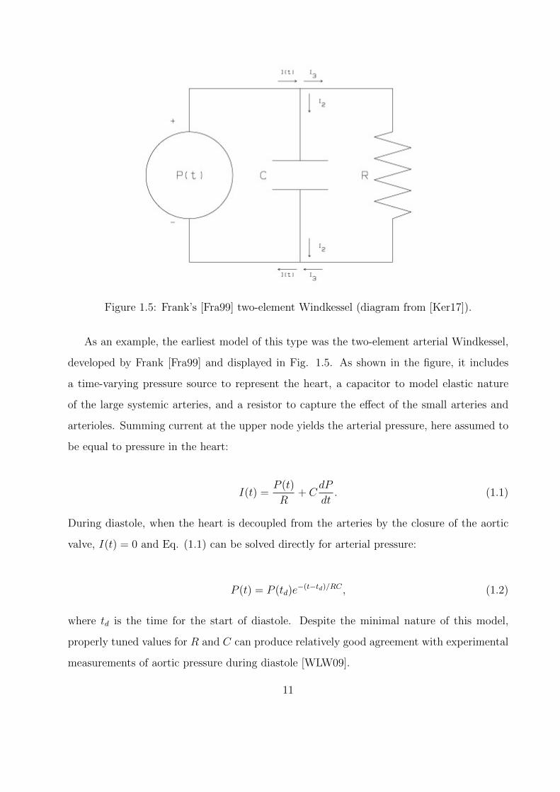
Figure 1.5: Frank’s [Fra99] two-element Windkessel (diagram from [Ker17]).

As an example, the earliest model of this type was the two-element arterial Windkessel,

developed by Frank [Fra99] and displayed in Fig. 1.5. As shown in the figure, it includes

a time-varying pressure source to represent the heart, a capacitor to model elastic nature

of the large systemic arteries, and a resistor to capture the effect of the small arteries and

arterioles. Summing current at the upper node yields the arterial pressure, here assumed to

be equal to pressure in the heart:

I(t) =P (t)

R+ C

dP

dt. (1.1)

During diastole, when the heart is decoupled from the arteries by the closure of the aortic

valve, I(t) = 0 and Eq. (1.1) can be solved directly for arterial pressure:

P (t) = P (td)e−(t−td)/RC , (1.2)

where td is the time for the start of diastole. Despite the minimal nature of this model,

properly tuned values for R and C can produce relatively good agreement with experimental

measurements of aortic pressure during diastole [WLW09].

11

Additions to the two-element Windkessel model have since been designed to incorporate

aortic valve resistance and the inertia of blood in the systemic arteries; a thorough historical

overview of these improvements can be found in Westerhof et al. [WLW09]. While these

modifications allow the behavior of the Windkessel to better match aortic pressure mea-

surements over the entire cardiac cycle, their spatial abstraction renders them insufficient

for providing local detail. In particular, these models cannot capture the wave transport

produced by elastic vessel wall motion [Moe77, Kor78], nor can they independently pro-

vide regional distributions of blood flow and pressure. Nonetheless, they are attractive for

their computational simplicity, and hence often find use as outflow boundary conditions for

higher-dimensional models, as further discussed in Sec. 1.2.2.

1.2.2 Higher-dimensional and multiscale modeling

To capture the wave motion omitted by lumped-parameter models, one-dimensional (or

“distributed”) models represent arterial segments by equations for viscous pulsatile flow in

an elastic tube. The solution to these equations for a single artery was first developed in

linearized form by Womersley [Wom57], who used Fourier series to obtain solutions in the

frequency domain. As computing power improved, this work was extended to the systemic

arterial tree to give localized vascular behavior in subsequent studies [WBD69, RJS74, Avo80,

WP04]. A significant drawback to these frequency-domain approaches is their assumption of

a periodic solution. This assumption is not justifiable when transient phenomena (e.g., those

produced by regulatory mechanisms) occur on timescales close to that of a cardiac cycle, as

is the case with baroreflex-mediated changes to heart rate and cardiac contractility [Dan98].

One-dimensional solutions in the time domain have also been developed based on both

quasilinear [SFP03, Ala06] and nonlinear [SA72, ZM86, SYR92, DNP03, VT04, FLT06,

RMP09] mass and momentum conservation averaged over vessel cross sections. Such solu-

tions necessarily involve numerical solution of systems of partial differential equations, and

are thus more computationally expensive than frequency domain approaches, which produce

algebraic relations between both pressures in different regions and pressure and flow rate at a

12

fixed location. However, time domain formulations do not require a periodic solution, making

them more amenable to coupling with regulatory models. Time-domain numerical solutions

to three-dimensional flows through patient-specific geometries also exist [TF09, BTF12], but

the present work focuses on reduced-order modeling, so this type of fully-resolved modeling

will not be further discussed.

Even in the limited context of one-dimensional models, the finer level of detail pro-

hibits global usage; it would not be feasible to discretize the complete O(108) meters of

systemic vasculature [LE04], and even if it were, flow in capillary beds cannot be mod-

eled through continuum techniques, as the lumen diameter becomes comparable to blood

cell size [TD09]. An efficient approach in this case is to employ multiscale modeling, in

which higher-dimensional subsystems representing domains of interest are coupled to lower-

dimensional subsystems at inflow and/or outflow boundaries. In one common architec-

ture, the major systemic arteries are treated as a one-dimensional network, and are cou-

pled to lumped-parameter models of the microcirculation, systemic veins, and left ventricle

[FLT06, RMP09, SYR92]. This subclass of models is open-loop, meaning that no consider-

ation is given to the return of blood to the heart. More complex extensions exist, including

one-dimensional venous networks [MT14], coupling to three-dimensional models of specific

arteries [QV03, KVF09, LBB11], and closed-loop models of heterogeneous dimensionality

[DNP03, OOT05, Goh07, LTH09a, LTH09b, BTF12, MVF13].

1.2.3 Regulatory control modeling

1.2.3.1 Baroreflex modeling

As discussed in Sec. 1.1.2, the sole neural regulatory mechanism relevant to this work is the

baroreflex, which can be split into three pieces for modeling purposes (see Fig. 1.4):

• The baroreceptors, for which the firing rate of nerve impulses sent to the cardiovascular

center are a function of arterial pressure (the “afferent” part)

13

• The cardiovascular center, which converts baroreceptor impulses into sympathetic and

parasympathetic nerve impulses

• The heart and vasculature, which change their behavior according to sympathetic and

parasympathetic stimulation (the “efferent” part)

Separate modeling of these parts has been extensively conducted over the past half cen-

tury (as reviewed by Danielsen [Dan98]), and is necessary for understanding the dynamics of

nerve impulses in response to different stimuli. Modeling can also be accomplished more sim-

ply by abstraction of the afferent firing rate [Dan98, BKS07]. This reduced implementation is

a two-step process: arterial pressure is converted directly into sympathetic/parasympathetic

activity, which in turn modulates lumped-parameter descriptions of the heart and vascu-

lature. This simplified model is attractive for this study, as it retains the influence of the

baroreflex on cardiovascular dynamics with minimal extraneous detail.

1.2.3.2 Autoregulatory modeling

With respect to cardiovascular autoregulation, a substantial share of modeling work in recent

years has focused on cerebral processes, as these localized processes are necessary to hold

cerebral blood flow constant under changing systemic blood pressure. This characteristic is

of particular interest to this work, as it counteracts the baroreflex; e.g., the baroreflex induces

global vasoconstriction when the baroreceptors detect low blood pressure, which requires an

opposing cerebral vasodilation to avoid reduced brain tissue perfusion. A model of this type

is therefore needed for accurate prediction of cerebrovascular responses to disease and injury.

As noted in the review by David and Moore [DM08], cerebral autoregulatory model-

ing can be broadly split into two categories: physiologically-based models that attempt

to mathematically describe autoregulatory processes, and empirical models that simply at-

tempt to fit experimental measurements of cerebral blood pressure and flow rate. The former

approach has the twin benefits of allowing for a better understanding of the underlying phys-

iology, and also being more readily applicable to lumped-parameter vascular models (i.e.,

the autoregulatory model can follow the baroreflex framework, driving changes in cerebral

14

resistance/compliance). For these reasons, the physiological approach will be pursued in this

work.

Akin to their cardiovascular counterparts, mathematical descriptions of cerebral autoreg-

ulation have been developed at varying levels of complexity. Banaji et al. [BTD05] provide

an example at the most resolved end of the spectrum, directly modeling processes from

the scale of ion transport up to the scale of the entire cerebral vasculature (the latter of

which is represented in lumped parameter form). Though elucidating physiological mecha-

nisms at such small scales can aid in understanding cellular mechanics, it is less crucial for

studying systemic cardiovascular responses. In these cases, cerebral autoregulation can be

modeled with less complexity by allowing changes in cerebral resistance and/or compliance

to be functions of deviations in cerebral pressure or blood flow from their reference values

[UD91]. This type of modeling is advantageous for the present study because it allows for

a direct, natural interaction between the cerebral vasculature’s fluid dynamics and its local

control mechanisms. Furthermore, it can be extended in a straightforward way to include

chemically-mediated responses by making the reference values functions of arterial carbon

dioxide concentration [LCG03].

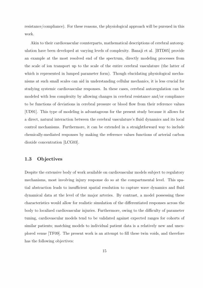
1.3 Objectives

Despite the extensive body of work available on cardiovascular models subject to regulatory

mechanisms, most involving injury response do so at the compartmental level. This spa-

tial abstraction leads to insufficient spatial resolution to capture wave dynamics and fluid

dynamical data at the level of the major arteries. By contrast, a model possessing these

characteristics would allow for realistic simulation of the differentiated responses across the

body to localized cardiovascular injuries. Furthermore, owing to the difficulty of parameter

tuning, cardiovascular models tend to be validated against expected ranges for cohorts of

similar patients; matching models to individual patient data is a relatively new and unex-

plored venue [TF09]. The present work is an attempt to fill these twin voids, and therefore

has the following objectives:

15

1. Develop a closed-loop model of the cardiovascular system with sufficient spatial reso-

lution to provide organ-level fluid dynamical data (i.e., pressure and flow rate in the

major arteries)

2. Couple the cardiovascular model to models of the baroreflex to allow for accurate

representation of dynamic responses to disease and injury

3. Leverage techniques from data assimilation [Eve03] to reduce computational cost and

enable patient-specific modeling

Chapters 2 and 3 focus on the first two objectives by detailing the implementation and

results for a full-body multiscale cardiovascular model with feedback control. Chapters 4

and 5 then address the final objective through construction and testing of a framework for

patient-specific modeling that generalizes across cardiovascular models. Finally, Chapter 6

concludes with a summary of accomplished goals and possible future directions.

16

CHAPTER 2

Construction of a Full-Scale Cardiovascular Model

As currently implemented, the overall model in this study couples zero-dimensional sub-

models of the heart, pulmonary vasculature, peripheral vasculature, and systemic veins with

a one-dimensional submodel of the systemic arteries. The zero-dimensional submodels are

in turn modulated by a baroreflex model. A high-level description of the connections be-

tween models is given in Fig. 2.1, followed by a complete connectivity diagram of the

one-dimensional network in Fig. 5.6. In this chapter, each submodel is described, and the

approach to 0D-1D coupling is outlined. Unless otherwise noted, numerical values for all

model parameters are reported at the end of the chapter.

2.1 Systemic arterial submodel

2.1.1 Basic model of a single artery

One-dimensional modeling of the major arteries essentially follows Sherwin et al. [SFP03],

but the main portions of their argument are reproduced here for clarity. Mass and momentum

conservation statements are derived from first principles using the control volume shown in

Fig. 2.3. In this control volume, quantities of interest are assumed to vary only in the

axial (x) direction, so the three dependent variables are cross-sectional area A = A(x, t),

u = u(x, t) (or equivalently volumetric flow rate Q = Au), and pressure P = P (x, t). The

flow is also assumed to be incompressible and Newtonian (i.e., ρ and µ are constants).

17

......

......

upper terminals

lower terminals

0D models 1D model

0D-1D

interfaces

baroreflex modelbaroreflex pressuresregulatory effects

pulmonary

circulationright

heart

left

heart

SVC

IVC

Figure 2.1: A high-level view of the closed-loop model architecture.

89 10

13 12

14

1116

1518

17 19

20

21

22

2425

27

26 28 29 3033

34 35

31

32

37

36

3839

40 41 42 43

4548

44

46 47

2

35

6

4

57

56

4950

51

5254

53

55

72

8687

89

8890

91

59

60

6162

63 64

65

66 68

69 70

67

1

73

71

7

74

75

76

7778 79

80

8185

82

83

84

23

58

Figure 2.2: Connectivity diagram of complete one-dimensional arterial network. Artery ID

numbers match tables found at the end of the chapter, while terminal annotations follow

Fig. 2.1.

18

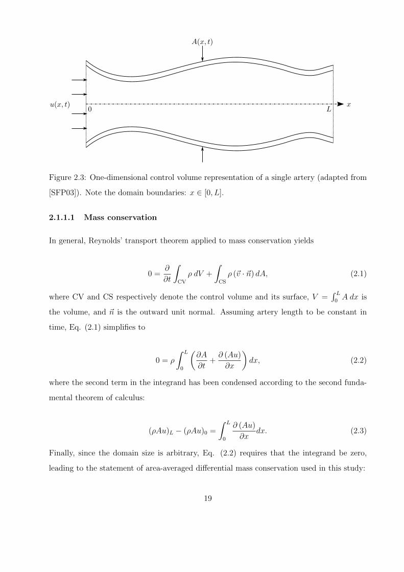
A(x, t)

u(x, t) x0 L

Figure 2.3: One-dimensional control volume representation of a single artery (adapted from

[SFP03]). Note the domain boundaries: x ∈ [0, L].

2.1.1.1 Mass conservation

In general, Reynolds’ transport theorem applied to mass conservation yields

0 =∂

∂t

∫CV

ρ dV +

∫CS

ρ (~v · ~n) dA, (2.1)

where CV and CS respectively denote the control volume and its surface, V =∫ L

0A dx is

the volume, and ~n is the outward unit normal. Assuming artery length to be constant in

time, Eq. (2.1) simplifies to

0 = ρ

∫ L

0

(∂A

∂t+∂ (Au)

∂x

)dx, (2.2)

where the second term in the integrand has been condensed according to the second funda-

mental theorem of calculus:

(ρAu)L − (ρAu)0 =

∫ L

0

∂ (Au)

∂xdx. (2.3)

Finally, since the domain size is arbitrary, Eq. (2.2) requires that the integrand be zero,

leading to the statement of area-averaged differential mass conservation used in this study:

19

∂A

∂t+∂ (Au)

∂x= 0. (2.4)

2.1.1.2 Momentum conservation

Momentum conservation again begins with Reynolds’ transport theorem, this time leading

to a balance between forces and momentum fluxes in the axial direction:

Fx =∂

∂t

∫ L

0

ρAu dx+

∫A(L,t)

ρu2 dA−∫A(0,t)

ρu2 dA (2.5)

The left-hand side is modeled as the sum of pressure forces at the ends of the segment,

integrated sidewall pressure force (projected into the axial direction), and an integrated

friction force per unit length f :

Fx = (PA)0 − (PA)L +

∫ L

0

(P∂A

∂x+ f

)dx. (2.6)

The momentum fluxes on the right-hand side of Eq. (2.5) can be integrated directly due to

the assumption of uniform flow at a fixed cross-section:

∫A(L,t)

ρu2 dA−∫A(0,t)

ρu2 dA = (ρu2A)L − (ρu2A)0. (2.7)

This momentum flux difference, along with the first two terms on the right-hand side of Eq.

(2.6), can be written in integral form akin to Eq. (2.3):

(ρu2A)L − (ρu2A)0 = ρ

∫ L

0

∂ (u2A)

∂xdx, (PA)0 − (PA)L = −

∫ L

0

∂ (PA)

∂xdx. (2.8)

Assuming arterial length to be independent of time, Eqs. (2.1) through (2.8) can be combined

under a single integral:

∫ L

0

[1

ρ

(−∂ (PA)

∂x+ P

∂A

∂x+ f

)−(∂ (uA)

∂t+∂ (u2A)

∂x

)]dx = 0. (2.9)

20

The second group in the integrand is simplified through expansion and application of Eq.

(2.4):

∂ (uA)

∂t+∂ (u2A)

∂x= A

[∂u

∂t+

∂

∂x

(u2

2

)]+ u��

��

�:0(∂A

∂t+∂ (Au)

∂x

). (2.10)

Now, since the integral in Eq. (2.9) must hold for an arbitrary control volume, the integrand

must be zero. Combining this conclusion with the result in Eq. (2.10) leads to the following

expression for differential momentum conservation in the axial direction:

∂u

∂t+

∂

∂x

(u2

2

)= −1

ρ

∂P

∂x+

f

ρA, (2.11)

where the pressure terms have been condensed through the product rule.

2.1.1.3 A constitutive relation, frictional modeling, and the complete system

To form a closed system for the unknowns A, u, and P , a starting point is to supplement

equations (2.4) and (2.11) with a constitutive relation between force perpendicular to the

vessel wall (i.e., pressure) and wall deformation (i.e., area). A common assumption is linear

elastic deformation [SFP03, Ala06, FLT06, LTH09a], from which Laplace’s law yields

P = β(√A−

√A0). (2.12)

In Eq. (2.12), β is a stiffness parameter relating the artery’s geometric and mechanical

properties:

β =

√πhE

(1− ν2)A0

, (2.13)

where h is wall thickness, E is Young’s modulus, A0 is the lumen cross-sectional area at

zero transmural pressure, and ν is Poisson’s ratio (wall incompressibility is assumed in this

study, so ν = 0.5). Lastly, a linear damping model for f is adopted from Alastruey [Ala06]

by assuming a nearly flat velocity profile (shown in vivo to be valid in the large arteries

[STL69]):

21

f = −22µπu. (2.14)

Finally, Eqs. (2.4) and (2.11) can be combined with Eqs. (2.12) through (2.14) to form a

complete system of equations in A and u:

∂U

∂t+∂F(U)

∂x= S,

U =

Au

, F(U) =

Au

β√A/ρ+ u2/2

, S =

0

−22πνu/A

, (2.15)

2.1.1.4 Characteristic form

The system given by Eqs. (2.15) can be placed into so-called “characteristic form” by first

writing it in non-conservative form [SFP03, Ala06]:

∂U

∂t+ H(U)

∂U

∂x= S,

H(U) =

u A

β/2ρ√A u

. (2.16)

The left eigenvectors L and associated matrix of eigenvalues Λ of H(U) (i.e., such that

LH = ΛL) are

L =

c/A 1

−c/A 1

, Λ =

u+ c 0

0 u− c

. (2.17)

Premultiplying Eq. (2.16) by L and defining a change of variables ∂W/∂U = L yields the

characteristic system

22

∂W

∂t+ Λ

∂W

∂x= LS,

W =

W1

W2

=

u+ 4√

β2ρ

(A1/4 − A1/40 )

u− 4√

β2ρ

(A1/4 − A1/40 )

=

u+ 4(c− c0)

u− 4(c− c0)

, (2.18)

whereW1,2 are the characteristic variables (or Riemann invariants). Note that the expressions

for W1 and W2 in Eqs. (2.18) can be combined to express area and average velocity as

A =

(2ρ

β

)2(W1 −W2

8+ co

)4

,

u =W1 +W2

2.

(2.19)

The relations (2.19) are important in the schemes for the 0D-1D boundaries as well as the

interior boundaries of the 1D network (i.e., at branching points).

2.1.2 Arterial numerical solution

2.1.2.1 Discretization of a single artery

To spatially discretize the system of equations (2.15), each arterial branch is split into eleven

uniformly-spaced nodes (i.e., for branch i with length L(i), ∆x(i) = L(i)/10). Local results

from grid refinement using 51 nodes per branch are presented for the longest artery in

Fig. 2.4. It was also confirmed that the global behavior of the model (as quantified in

Table 3.2) varied by less than 1% across all measured parameters under refinement. For

time discretization, the CFL was fixed at 0.5, and ∆t was chosen to satisfy this constraint

according to the following minimization:

∆t = mini

(CFL∆x(i)

c(i)0

), (2.20)

where c0 is the pulse wave velocity at zero transmural pressure:

23

0 0.1 0.2 0.3 0.4 0.5 0.6 0.7 0.8 0.9

t (sec)

50

60

70

80

90

100

110

120

130

140P

(m

mH

g)

Pressure comparison in artery 31 (L = 16.1 cm)

51 nodes

11 nodes

0 0.1 0.2 0.3 0.4 0.5 0.6 0.7 0.8 0.9

t (sec)

1

2

3

4

5

6

7

Q (

mL/s

)

Flow comparison in artery 31 (L = 16.1 cm)

51 nodes

11 nodes

Figure 2.4: Selected localized results from a grid refinement study in the one-dimensional

arterial network.

c0 =

√β

2ρA

1/40 . (2.21)

With the above discretization, each artery’s interior nodes are advanced in time using a

3rd-order TVD Runge-Kutta/CWENO method [SO88, NKS17] applied to Eqs. (2.15).

2.1.2.2 Interior boundaries (arterial branching)

The systemic arteries constitute a branching network in which a parent vessel divides into

two or more daughter vessels. Fig. 2.5 illustrates the model for these divisions. At such a

junction, continuity of mass flow and total pressure Pt = P+ 12ρ(Q/A)2 are imposed [FLT06].

For a parent vessel of index p with children c1, c2, . . . , cm, doing so yields

Q(n+1)p = Q(n+1)

c1+Q(n+1)

c2+ . . .+Q(n+1)

cm

P(n+1)t,p = P

(n+1)t,c1 = P

(n+1)t,c2 = . . . = P

(n+1)t,cm ,

(2.22)

where n denotes the current time step.

The nonlinear algebraic system (2.22) has m + 1 equations in 2(m + 1) unknowns (the

24

Q(n+1)p Q

(n+1)ci

Q(n+1)c1

Q(n+1)cm

W(n+1)1,p W

(n+1)2,ci

W(n+1)2,c1

W(n+1)2,cm

P(n+1)t

Figure 2.5: Schematic of an arterial splitting node. The index i ranges from 1 to m, the

number of children at the split, while the index n denotes the current time step. In the

spatial discretization, the parent’s most distal node coincides with the most proximal node

of each child.

flow rate/area pairs for each vessel). For closure, the characteristic variables W1,2 presented

in Eqs. (2.18) are employed. These characteristic variables travel with velocities

λ1,2 =Q

A±

√β

2ρA1/4 = u± c. (2.23)

Under physiological conditions, u � c, so W1,2 will always travel forwards and backwards,

respectively. As such, W1 can be extrapolated forward from the interior of the parent artery,

and W2 backwards from each of the children. Concretely, assuming the parent artery to have

a length Lp gives

W(n+1)1,p (x = Lp) = W

(n)1 (x = Lp − λ(n)

1 ∆t)− 22πνu(n)(x = Lp − λ(n)

1 ∆t)

A(n)(x = Lp − λ(n)1 ∆t)

W(n+1)2,c (x = 0) = W

(n)2 (x = −λ(n)

2 ∆t)− 22πνu

(n)c (x = −λ(n)

2 ∆t)

A(n)c (x = −λ(n)

2 ∆t),

(2.24)

where W(n)1,2 are calculated by interpolating between the last two nodes of the parent and the

25

first two nodes of each child. Equations (2.22) and (2.24) form a closed nonlinear algebraic

system in 2(m+ 1) unknowns, and are solved iteratively using Newton’s method.

2.2 Cardiac submodel

The heart model implemented in this study belongs to a class of lumped-parameter models

known as “elastance” models, first proposed by Suga et al. [SSS73] and commonly used

in other works [Dan98, OD03, OOT05, FLT06, Goh07, KVF09, LTH09b, LTH09a, RMP09,

MDP12, BTF12, MT14]. In the following description, the subscript v represents either

ventricle, while the subscript a represents either atrium. Also, for some equations it is

necessary to define a time within a heart period t = mod(t, th), where th = 1/f0 is the

heart period. In this model, the left and right ventricles are represented as pressure-volume

relationships of the form

Pv = Ev(t)(Vv − Vv,un), (2.25)

where Vv is ventricular volume, Vv,un is a modeling parameter representing volume at zero di-

astolic pressure (sometimes called unstressed volume), and Ev(t) is a time-varying elastance

intended to model ventricular pumping. Given a minimum diastolic elastance Emin and max-

imum systolic elastance Emax, it is defined using the ‘two-Hill’ function [SMW96, MDP12]

Ev(t) = k

(g1

1 + g1

)(1

1 + g2

)+ Emin, (2.26)

where g1 and g2 describe each ‘hill’

g1 =

(t

τ1

)m1

, g2 =

(t

τ2

)m2

, (2.27)

and k scales their product:

k =Emax − Emin

max[(

g11+g1

)(1

1+g2

)] . (2.28)

26

0 0.1 0.2 0.3 0.4 0.5 0.6 0.7 0.8 0.9 1

0

0.2

0.4

0.6

0.8

1

1.2

Ev(t)

g11+g1

11+g2

t/th

Normalized

values

systole diastole

Figure 2.6: A typical ventricular elastance curve from the ‘two-Hill’ function alongside its

component Hill functions. Each curve has been normalized by its maximum value. The

vertical dashed line demarcates the systolic and diastolic phases.

A typical elastance curve and constituent Hill functions are shown in Fig. 2.6, illustrating

the gradual rise in elastance (and hence ventricular pressure) during systole, followed by a

sharp fall in both quantities during early diastole.

Atrial pressures are described using the same form as Eq. (2.25), except that elastance

is taken as a constant (i.e., the atria are modeled as passive elastic chambers). More com-

plex compartmental models accounting for atrial contraction are available [BTF12, LTH09a,

LTH09b], but their effects on systemic arterial hemodynamics are negligible: atrial systole

occurs within ventricular diastole, during which the left ventricle and systemic arteries are

decoupled. Since this study is concerned with local hemodynamics only in the systemic

circulation, this modeling aspect is omitted for computational simplicity.

To determine the time evolution of ventricular volume, conservation of mass for an in-

compressible fluid is applied:

dVvdt

= Qa −Qv, (2.29)

27

where Qa and Qv denote atrial and ventricular flow rates, respectively. Note that these

flow rates can be nonzero only when the appropriate heart valves are open. To model

atrioventricular valve closure, atrial flow rates are set to zero when Pv exceeds Pa. For the

right ventricle only, the pulmonary valve is closed once Qv becomes negative (aortic valve

modeling is discussed in Sec. 2.5.1). Atrial volumes are determined in a fashion similar to

Eq. (2.29):

dVadt

= Qve −Qa, (2.30)

where Qve indicates the rate of venous return. For the right atrium, this return is determined

from the peripheral vascular model as the sum of the flows through lumped-parameter com-

partments representing the inferior and superior vena cavae. By contrast, the left atrium’s

venous return is taken as the flow rate through the second venous compartment of the pul-

monary vascular model. Atrioventricular flow rates are determined by the following evolution

equation:

dQa

dt=

1

La(Pa − Pv)−

Ra

LaQa, (2.31)

where La represents inductance and Ra is atrial resistance.

For the right ventricle only, the flow rate advances in time as

dQrv

dt=

1

Lrv(Prv − Pe), (2.32)

where Lv is the inductance and Pe is the pulmonary arterial pressure into which the right

ventricle ejects:

Pe = ReQrv + P1, (2.33)

where Re is the pulmonary artery’s resistance and P1 is the pressure in the most proximal

compartment of the pulmonary circulation. Note that the flow rate out of the left ventricle

is not determined in a manner analogous to Eq. (2.32) when the aortic valve is opened.

28

Rather, it is determined by coupling to the systemic 1D model, as described in Sec. 2.5.1.

Finally, all time evolutions described in this section are discretized using the forward Euler

method.

2.3 Pulmonary submodel

The pulmonary circulation is subdivided into five lumped-parameter compartments charac-

terized by linear circuit elements, following the work of Danielsen [Dan98]. In the following

description, subscripts ranging from 1 to 5 indicate movement from the large arteries to the

large veins. In all five compartments, volume changes according to conservation of mass:

dV1

dt= Qv −Q1,

dVidt

= Qi−1 −Qi i = 2, . . . , 5.

(2.34)

In the first and fifth compartments, an inductance is included to model the inertia of blood

within the large arteries and veins. As such, the flow rate in these sections are given by

dQi

dt=

1

Li(Pi − Pi+1)− Ri

LiQi. i = 1, 5, (2.35)

where Ri is compartmental resistance and Li is inductance. The middle compartments

contain only a resistance (i.e., viscous effects are assumed to dominate inertial effects, as is

the case in small vessels and capillaries [TD09]), resulting in simple algebraic relations for

the flow rate:

Qi =Pi − Pi+1

Ri

, i = 2, 3, 4. (2.36)

Finally, each compartment is assumed to deform passively, resulting in the following rela-

tionships for pressure:

Pi =1

Ci(Vi − Vi,un), i = 1, . . . , 5, (2.37)

29

Q0,unu

C1u

R1u,unu

P1,unu

Q1,unu

C2u

R2u

P2,unu

Q2,unu

C3u

R3u

P3,unu

Q3,unu

C4u

R4u

P4,unu

Q4,unu

C5u

R5u

P5,unu

Q5,unu

L5u

Q0,u1

C1u

R1u,u1

P1,u1

Q1,u1

C2u

R2u

P2,u1

Q2,u1

C3u

R3u

P3,u1

Q3,u1

C4u

R4u

P4,u1

Q4,u1

C5u

R5u

P5,u1

Q5,u1

L5u

CSVC

RSVC LSVC

PSVCQSVC

PraQ5,ui

Figure 2.7: Schematic of the compartments representing the upper peripheral circulation

and superior vena cava. The second subscript u indicates an upper terminal artery, with

the associated index i running from 1 to the number of upper body terminal arteries nu.

The lower compartments and inferior vena cava have an identical structure. The left-hand

terminals are connected to 1D arterial domains, while the right-hand terminal is connected

to the right atrium.

where the last terms in each equation represent unstressed volumes, and each parameter Ci

denotes the compliance of that compartment. As with the cardiac submodel, equations are

discretized using the forward Euler method where necessary.

2.4 Peripheral submodel

To save computational effort, the 1D network only explicitly models 91 of the largest arteries

in the systemic vasculature. However, it is still necessary to account for the hemodynamic

effects of the smaller arteries, arterioles, capillary beds, and venous network. To do so,

all terminal arteries (i.e., arteries that do not branch into explicitly represented daughter

vessels) are coupled to zero-dimensional models similar to those used for the pulmonary

circulation. In total, each terminal artery is associated with five terminal compartments,

as illustrated in Fig. 2.7. Each compartment’s volume is determined by conservation of

mass, similarly to Eq. (2.34), with the most proximal incoming flow rate determined by

iterative coupling to the 1D model (see Sec. 2.5.2). Compartmental pressures relate to

volume through capacitance as in Eq. (2.37), and flow rates in the four most proximal

30

compartments relate to pressure differences analogously to Eq. (2.36). The most distal

compartment includes an inductance for the large veins, so its flow rate changes akin to Eq.

(2.35). These distal compartments then connect to appropriate vena caval compartments

(e.g., upper body terminal compartments connect to the superior vena caval compartments),

whose pressures and flow rates are calculated following Eqs. (2.37) and (2.35).

2.5 0D-1D coupling

To couple the 1D model of the major arteries to the compartmental models for the remaining

cardiovascular system, an iterative approach based on the work of Liang et al. [LTH09a] is

employed. This method makes use of Eqs. (2.19), which show that W1,2 completely specify

A and u at a node, and the fact that W1,2 can be extrapolated from interior nodes of the 1D

domain by following characteristic lines [SFP03, Ala06, LTH09a].

2.5.1 Proximal coupling

At the proximal boundary of the 1D network, in the event that the aortic valve is closed

(i.e., during diastole), it is necessary to enforce Qlv = 0. From Eqs. (2.19), this condition

requires W1 = −W2 , leading to the following time advancement scheme:

1. Update W2 at the boundary by extrapolating from interior nodes:

W(n+1)2,ao (x = 0) = W

(n)2,ao(x = −λ(n)

2 ∆t)− 22πνu

(n)ao (x = −λ(n)

2 ∆t)

A(n)ao (x = −λ(n)

2 ∆t). (2.38)

2. Set W1 so that Qlv = 0:

W(n+1)1,ao (x = 0) = −W (n+1)

2,ao (x = 0). (2.39)

3. Update A at the proximal boundary according to Eqs. (2.19):

A(n+1)ao (x = 0) =

(2ρ

βao

)2(W

(n+1)1,ao (x = 0)−W (n+1)

2,ao (x = 0)

8+ c0,ao

)4

(2.40)

31

4. Finally, update the left ventricular state using a forward Euler discretization of Eq.

(2.29) (noting Qlv = 0 during diastole):

V(n+1)lv = V

(n)lv + ∆tQ

(n)la ,

P(n+1)lv = E

(n+1)lv (V

(n+1)lv − Vlv,un).

(2.41)

Note that this process allows decoupling of the left ventricle from the aorta during dias-

tole (i.e., no ventricular outflow) while still allowing for wave reflections from the proximal

boundary within the 1D domain [FLT06].

In contrast to the closed valve condition outlined above, the open valve condition fully

couples the left ventricle and systemic arteries. To do so, a variant of the aortic valve model

proposed by Mynard et al. [MDP12] is employed. In this model, the pressure drop across

the valve accounts for viscous, inertial, and ‘Bernoulli’ losses:

Plv − Pao = BQlv|Qlv|+ LdQlv

dt+RQlv, (2.42)

where B and L depend on the effective orifice area Aeff:

B =ρ

2A2eff

, L =ρleff

Aeff

, (2.43)

and leff is a constant characteristic length scale for flow across the valve. Aeff varies with

time according to a valve state index ζ, 0 ≤ ζ ≤ 1:

Aeff = Aannζ(t), (2.44)

where Aann is the maximum transvalvular area and ζ changes according to its current state

and the transvalvular pressure difference ∆P = Plv − Pao:

dζ

dt= (1− ζ)Kvo∆P, ∆P > 0

dζ

dt= ζKvc∆P, ∆P < 0.

(2.45)

32

In Eq. (2.45), Kvo and Kvc are rate constants for valve opening and closing, respectively. A

backward Euler discretization of Eqs. (2.42) and (2.45), along with a similar discretization

of Eq. (2.29), the constitutive relations in Eqs. (2.12) and (2.25), and the characteristic

relations in Eq. (2.19) are solved simultaneously using Newton-Raphson iteration and the

extrapolated interior characteristic from Eq. (2.38). Coupling in this manner allows for wave

interactions between the left ventricle and the systemic arterial network [FLT06].

2.5.2 Distal coupling

At the distal end of the 1D network, terminal arteries are coupled to the most proximal 0D

compartment outlined in Sec. 2.4. To do so, the process is very similar to the open valve

conditions for the proximal 1D boundary, except that the characteristic variable leaving the

1D domain is W1, rather than W2. In this case, an algebraic system is formed from the

characteristic relations given in Eq. (2.19), the constitutive relations in Eqs. (2.37) and

(2.12), and a semi-implicit discretization of mass conservation:

V(n+1)

1 = V n1 + ∆t(Q

(n+1)1D −Qn

1 ) (2.46)

This algebraic system is solved at each distal coupling point using the Newton-Raphson

method and W1 extrapolated from the 1D domain in a manner analogous to Eq. (2.24).

2.6 Baroreflex submodel

To simulate regulation by the central nervous system in the 0D models, a modified version

of the model developed by Danielsen [Dan98] and extended by Blanco et al. [BTF12] is

implemented. First, an average pressure over all the baroreflex sites is defined as an activation

signal:

Pbaro =1

3th

(∫ th

0

Paa(x = 0) dt+

∫ th

0

Plc(x = 0) dt+

∫ th

0

Prc(x = 0) dt

), (2.47)

33

0 0.2 0.4 0.6 0.8 1 1.2 1.4 1.6 1.8 2

0

0.1

0.2

0.3

0.4

0.5

0.6

0.7

0.8

0.9

1

Pbaroψ

Autonom

icactivation

ηsηp

Figure 2.8: Illustration of autonomic activation functions. Asymmetry about target barore-

ceptor pressure follows [Kor71].

where the subscripts aa, lc, and rc denote the aortic arch, the left carotid, and the right

carotid. By using pressure as the afferent signal in this manner, afferent nerve impulse

dynamics are omitted for simplicity. The sympathetic and parasympathetic tones are then

described as asymmetric sigmoidal functions of the baroreflex pressure Pbaro:

ηs = exp

{−aηexp

[bη

(Pbaro

ψ− 1

)]},

ηp = exp

{−aηexp

[−bη

(Pbaro

ψ− 1

)]}.

(2.48)

In Eq. (2.48), the constant ψ is the target mean pressure at the baroreceptors, aη charac-

terizes the firing rate at this pressure (Pbaro = ψ), and bη characterizes sigmoidal steepness.

This approach is based on experimental observations by Korner [Kor71], and is illustrated in

Fig. 2.8. Importantly, the asymmetry about the target point allows a higher maximum heart

rate while still preserving physiological levels of extreme bradycardia (i.e., low heart rates).

These extrema, as well as the extrema for all other controlled parameters, are displayed in

Table 2.1.

34

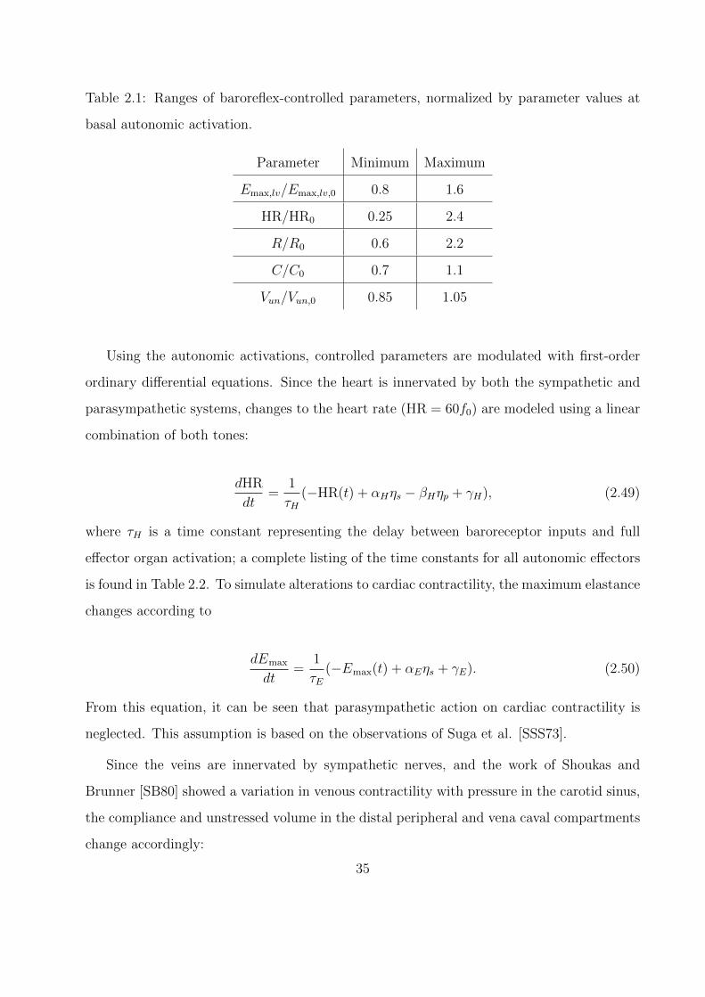
Table 2.1: Ranges of baroreflex-controlled parameters, normalized by parameter values at

basal autonomic activation.

Parameter Minimum Maximum

Emax,lv/Emax,lv,0 0.8 1.6

HR/HR0 0.25 2.4

R/R0 0.6 2.2

C/C0 0.7 1.1

Vun/Vun,0 0.85 1.05

Using the autonomic activations, controlled parameters are modulated with first-order

ordinary differential equations. Since the heart is innervated by both the sympathetic and

parasympathetic systems, changes to the heart rate (HR = 60f0) are modeled using a linear

combination of both tones:

dHR

dt=

1

τH(−HR(t) + αHηs − βHηp + γH), (2.49)

where τH is a time constant representing the delay between baroreceptor inputs and full

effector organ activation; a complete listing of the time constants for all autonomic effectors

is found in Table 2.2. To simulate alterations to cardiac contractility, the maximum elastance

changes according to

dEmax

dt=

1

τE(−Emax(t) + αEηs + γE). (2.50)

From this equation, it can be seen that parasympathetic action on cardiac contractility is

neglected. This assumption is based on the observations of Suga et al. [SSS73].

Since the veins are innervated by sympathetic nerves, and the work of Shoukas and

Brunner [SB80] showed a variation in venous contractility with pressure in the carotid sinus,

the compliance and unstressed volume in the distal peripheral and vena caval compartments

change accordingly:

35

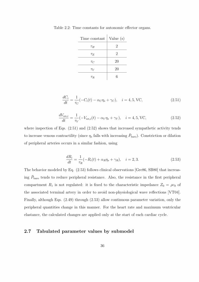
Table 2.2: Time constants for autonomic effector organs.

Time constant Value (s)

τH 2

τE 2

τC 20

τV 20

τR 6

dCidt

=1

τC(−Ci(t)− αCηs + γC), i = 4, 5,VC, (2.51)

dVun,idt

=1

τV(−Vun,i(t)− αV ηs + γV ), i = 4, 5,VC, (2.52)

where inspection of Eqs. (2.51) and (2.52) shows that increased sympathetic activity tends

to increase venous contractility (since ηs falls with increasing Pbaro). Constriction or dilation

of peripheral arteries occurs in a similar fashion, using

dRi

dt=

1

τR(−Ri(t) + αRηs + γR), i = 2, 3. (2.53)

The behavior modeled by Eq. (2.53) follows clinical observations [Gre86, SB80] that increas-

ing Pbaro tends to reduce peripheral resistance. Also, the resistance in the first peripheral

compartment R1 is not regulated: it is fixed to the characteristic impedance Z0 = ρc0 of

the associated terminal artery in order to avoid non-physiological wave reflections [VT04].

Finally, although Eqs. (2.49) through (2.53) allow continuous parameter variation, only the

peripheral quantities change in this manner. For the heart rate and maximum ventricular

elastance, the calculated changes are applied only at the start of each cardiac cycle.

2.7 Tabulated parameter values by submodel

36

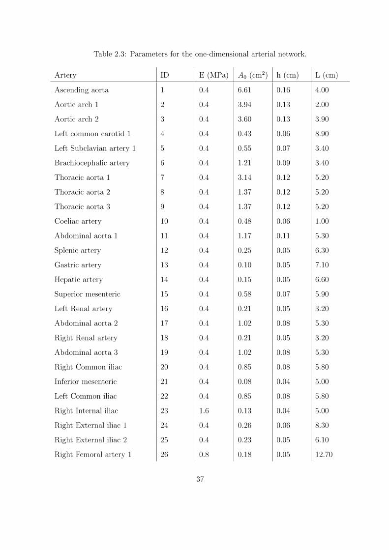
Table 2.3: Parameters for the one-dimensional arterial network.

Artery ID E (MPa) A0 (cm2) h (cm) L (cm)

Ascending aorta 1 0.4 6.61 0.16 4.00

Aortic arch 1 2 0.4 3.94 0.13 2.00

Aortic arch 2 3 0.4 3.60 0.13 3.90

Left common carotid 1 4 0.4 0.43 0.06 8.90

Left Subclavian artery 1 5 0.4 0.55 0.07 3.40

Brachiocephalic artery 6 0.4 1.21 0.09 3.40

Thoracic aorta 1 7 0.4 3.14 0.12 5.20

Thoracic aorta 2 8 0.4 1.37 0.12 5.20

Thoracic aorta 3 9 0.4 1.37 0.12 5.20

Coeliac artery 10 0.4 0.48 0.06 1.00

Abdominal aorta 1 11 0.4 1.17 0.11 5.30

Splenic artery 12 0.4 0.25 0.05 6.30

Gastric artery 13 0.4 0.10 0.05 7.10

Hepatic artery 14 0.4 0.15 0.05 6.60

Superior mesenteric 15 0.4 0.58 0.07 5.90

Left Renal artery 16 0.4 0.21 0.05 3.20

Abdominal aorta 2 17 0.4 1.02 0.08 5.30

Right Renal artery 18 0.4 0.21 0.05 3.20

Abdominal aorta 3 19 0.4 1.02 0.08 5.30

Right Common iliac 20 0.4 0.85 0.08 5.80

Inferior mesenteric 21 0.4 0.08 0.04 5.00

Left Common iliac 22 0.4 0.85 0.08 5.80

Right Internal iliac 23 1.6 0.13 0.04 5.00

Right External iliac 1 24 0.4 0.26 0.06 8.30

Right External iliac 2 25 0.4 0.23 0.05 6.10

Right Femoral artery 1 26 0.8 0.18 0.05 12.70

37

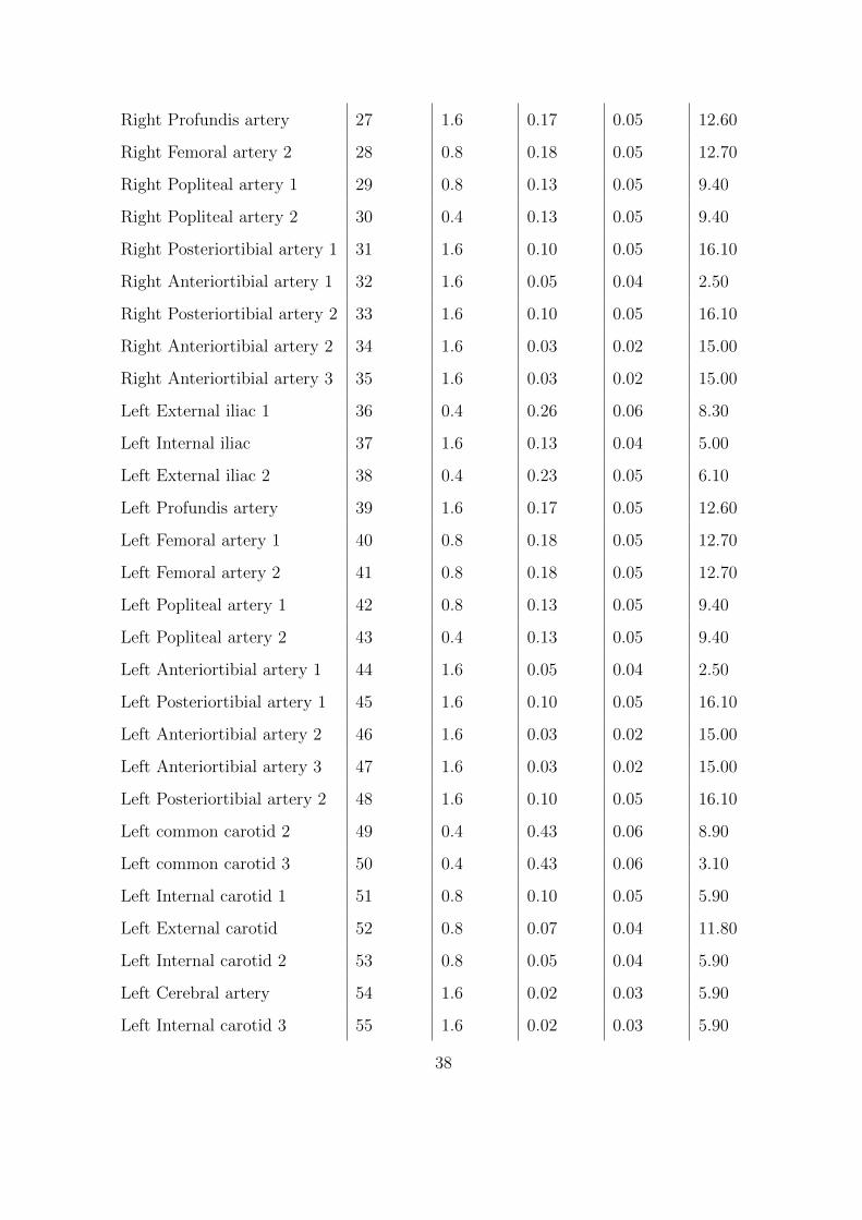
Right Profundis artery 27 1.6 0.17 0.05 12.60

Right Femoral artery 2 28 0.8 0.18 0.05 12.70

Right Popliteal artery 1 29 0.8 0.13 0.05 9.40

Right Popliteal artery 2 30 0.4 0.13 0.05 9.40

Right Posteriortibial artery 1 31 1.6 0.10 0.05 16.10

Right Anteriortibial artery 1 32 1.6 0.05 0.04 2.50

Right Posteriortibial artery 2 33 1.6 0.10 0.05 16.10



Left External iliac 1 36 0.4 0.26 0.06 8.30

Left Internal iliac 37 1.6 0.13 0.04 5.00

Left External iliac 2 38 0.4 0.23 0.05 6.10

Left Profundis artery 39 1.6 0.17 0.05 12.60

Left Femoral artery 1 40 0.8 0.18 0.05 12.70

Left Femoral artery 2 41 0.8 0.18 0.05 12.70

Left Popliteal artery 1 42 0.8 0.13 0.05 9.40

Left Popliteal artery 2 43 0.4 0.13 0.05 9.40

Left Anteriortibial artery 1 44 1.6 0.05 0.04 2.50

Left Posteriortibial artery 1 45 1.6 0.10 0.05 16.10



Left Posteriortibial artery 2 48 1.6 0.10 0.05 16.10



Left Internal carotid 1 51 0.8 0.10 0.05 5.90

Left External carotid 52 0.8 0.07 0.04 11.80


Left Cerebral artery 54 1.6 0.02 0.03 5.90


38

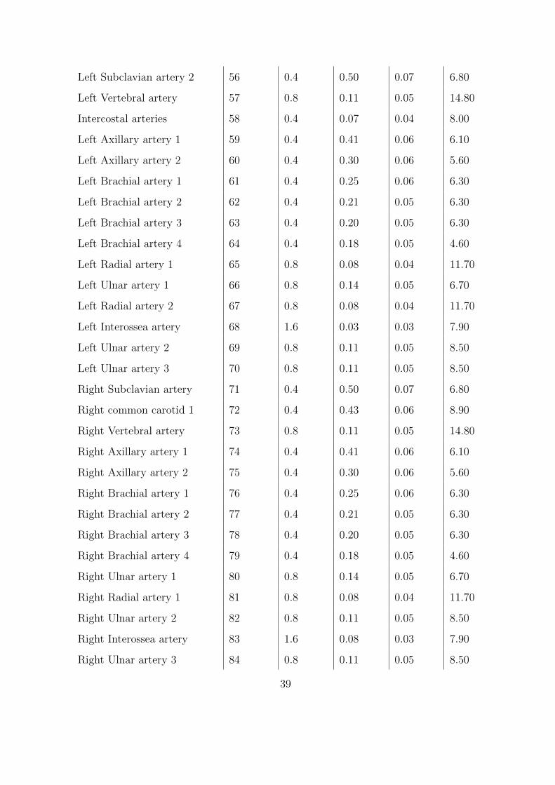
Left Subclavian artery 2 56 0.4 0.50 0.07 6.80

Left Vertebral artery 57 0.8 0.11 0.05 14.80

Intercostal arteries 58 0.4 0.07 0.04 8.00

Left Axillary artery 1 59 0.4 0.41 0.06 6.10

Left Axillary artery 2 60 0.4 0.30 0.06 5.60

Left Brachial artery 1 61 0.4 0.25 0.06 6.30




Left Radial artery 1 65 0.8 0.08 0.04 11.70

Left Ulnar artery 1 66 0.8 0.14 0.05 6.70

Left Radial artery 2 67 0.8 0.08 0.04 11.70

Left Interossea artery 68 1.6 0.03 0.03 7.90



Right Subclavian artery 71 0.4 0.50 0.07 6.80

Right common carotid 1 72 0.4 0.43 0.06 8.90

Right Vertebral artery 73 0.8 0.11 0.05 14.80

Right Axillary artery 1 74 0.4 0.41 0.06 6.10

Right Axillary artery 2 75 0.4 0.30 0.06 5.60

Right Brachial artery 1 76 0.4 0.25 0.06 6.30




Right Ulnar artery 1 80 0.8 0.14 0.05 6.70

Right Radial artery 1 81 0.8 0.08 0.04 11.70


Right Interossea artery 83 1.6 0.08 0.03 7.90


39

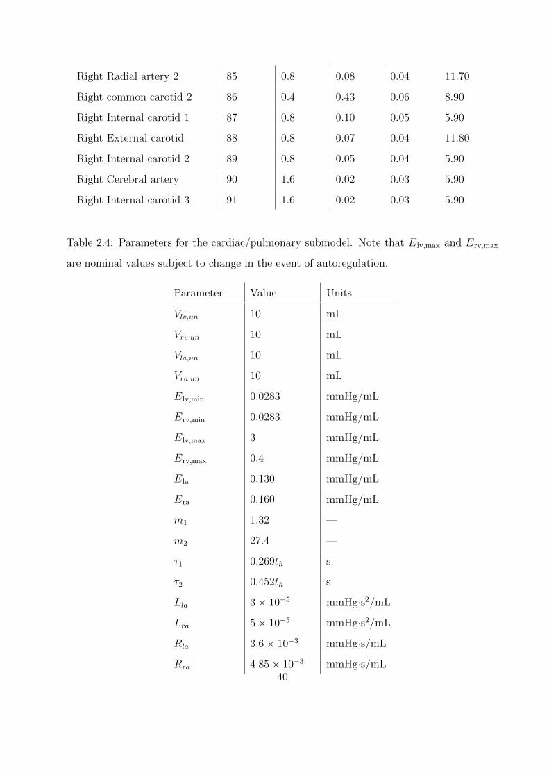
Right Radial artery 2 85 0.8 0.08 0.04 11.70

Right common carotid 2 86 0.4 0.43 0.06 8.90

Right Internal carotid 1 87 0.8 0.10 0.05 5.90

Right External carotid 88 0.8 0.07 0.04 11.80


Right Cerebral artery 90 1.6 0.02 0.03 5.90


Table 2.4: Parameters for the cardiac/pulmonary submodel. Note that Elv,max and Erv,max

are nominal values subject to change in the event of autoregulation.

Parameter Value Units

Vlv,un 10 mL

Vrv,un 10 mL

Vla,un 10 mL

Vra,un 10 mL

Elv,min 0.0283 mmHg/mL

Erv,min 0.0283 mmHg/mL

Elv,max 3 mmHg/mL

Erv,max 0.4 mmHg/mL

Ela 0.130 mmHg/mL

Era 0.160 mmHg/mL

m1 1.32 —

m2 27.4 —

τ1 0.269th s

τ2 0.452th s

Lla 3× 10−5 mmHg·s2/mL

Lra 5× 10−5 mmHg·s2/mL

Rla 3.6× 10−3 mmHg·s/mL

Rra 4.85× 10−3 mmHg·s/mL40

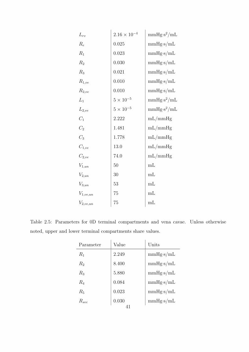
Lrv 2.16× 10−4 mmHg·s2/mL

Re 0.025 mmHg·s/mL

R1 0.023 mmHg·s/mL

R2 0.030 mmHg·s/mL

R3 0.021 mmHg·s/mL

R1,ve 0.010 mmHg·s/mL

R2,ve 0.010 mmHg·s/mL

L1 5× 10−5 mmHg·s2/mL

L2,ve 5× 10−5 mmHg·s2/mL

C1 2.222 mL/mmHg

C2 1.481 mL/mmHg

C3 1.778 mL/mmHg

C1,ve 13.0 mL/mmHg

C2,ve 74.0 mL/mmHg

V1,un 50 mL

V2,un 30 mL

V3,un 53 mL

V1,ve,un 75 mL

V2,ve,un 75 mL

Table 2.5: Parameters for 0D terminal compartments and vena cavae. Unless otherwise

noted, upper and lower terminal compartments share values.


R1 2.249 mmHg·s/mL

R2 8.400 mmHg·s/mL

R3 5.880 mmHg·s/mL

R4 0.084 mmHg·s/mL

R5 0.023 mmHg·s/mL

Rsvc 0.030 mmHg·s/mL41

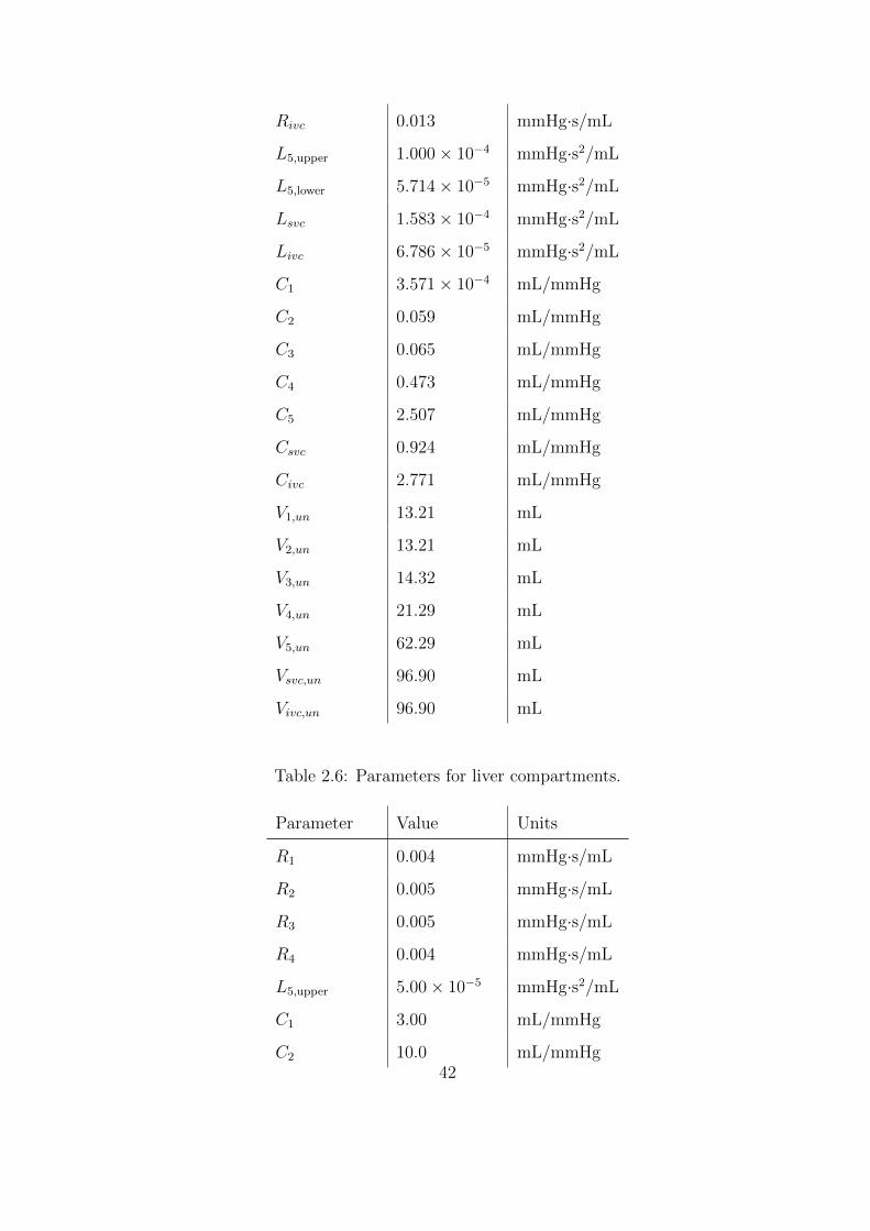
Rivc 0.013 mmHg·s/mL

L5,upper 1.000× 10−4 mmHg·s2/mL

L5,lower 5.714× 10−5 mmHg·s2/mL

Lsvc 1.583× 10−4 mmHg·s2/mL

Livc 6.786× 10−5 mmHg·s2/mL

C1 3.571× 10−4 mL/mmHg

C2 0.059 mL/mmHg

C3 0.065 mL/mmHg

C4 0.473 mL/mmHg

C5 2.507 mL/mmHg

Csvc 0.924 mL/mmHg

Civc 2.771 mL/mmHg

V1,un 13.21 mL

V2,un 13.21 mL

V3,un 14.32 mL

V4,un 21.29 mL

V5,un 62.29 mL

Vsvc,un 96.90 mL

Vivc,un 96.90 mL

Table 2.6: Parameters for liver compartments.


R1 0.004 mmHg·s/mL

R2 0.005 mmHg·s/mL

R3 0.005 mmHg·s/mL

R4 0.004 mmHg·s/mL

L5,upper 5.00× 10−5 mmHg·s2/mL

C1 3.00 mL/mmHg

C2 10.0 mL/mmHg42

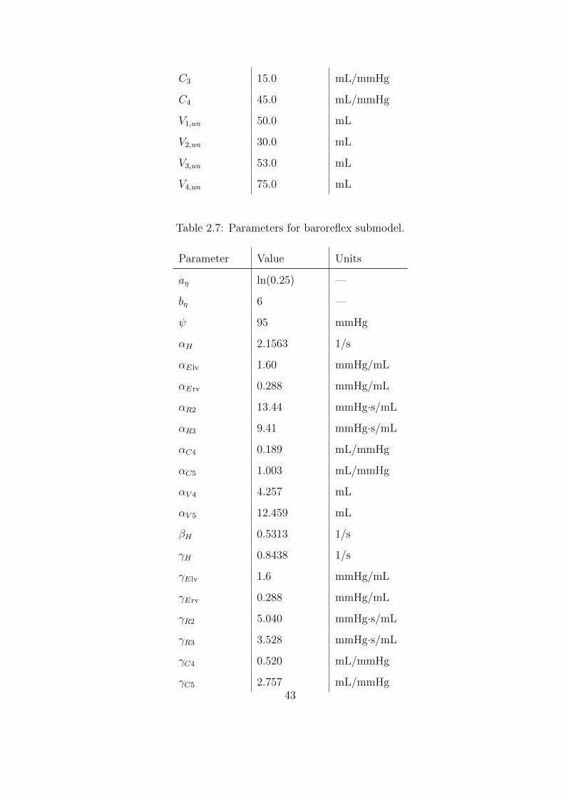
C3 15.0 mL/mmHg

C4 45.0 mL/mmHg

V1,un 50.0 mL

V2,un 30.0 mL

V3,un 53.0 mL

V4,un 75.0 mL

Table 2.7: Parameters for baroreflex submodel.


aη ln(0.25) —

bη 6 —

ψ 95 mmHg

αH 2.1563 1/s

αE lv 1.60 mmHg/mL

αErv 0.288 mmHg/mL

αR2 13.44 mmHg·s/mL

αR3 9.41 mmHg·s/mL

αC4 0.189 mL/mmHg

αC5 1.003 mL/mmHg

αV 4 4.257 mL

αV 5 12.459 mL

βH 0.5313 1/s

γH 0.8438 1/s

γE lv 1.6 mmHg/mL

γErv 0.288 mmHg/mL

γR2 5.040 mmHg·s/mL

γR3 3.528 mmHg·s/mL

γC4 0.520 mL/mmHg

γC5 2.757 mL/mmHg43

γV 4 22.35 mL

γV 5 65.41 mL

44

CHAPTER 3

Full-Scale Model Results and Analysis

3.1 Validation under resting conditions

As validation, selected results from the periodic steady state under resting conditions (i.e.,

with basal levels of autonomic activation) are presented. Table 3.1 compares regional blood

flow predicted by the model to experimental data. This comparison shows that the 1D model

is able to accurately capture the localized distribution of cardiac output. Fig. 3.1 displays the

spatial and temporal evolution of the pressure waveform as it leaves the heart and travels into

the left leg. The amplitude of the pressure wave first decreases, then increases with distance

from the heart, as measured by the widening gap between systolic and diastolic pressures.

The increase in systolic pressure corresponds to the gradual narrowing of the aorta as it

descends the abdomen, with the peak occuring near the aortic bifurcation. This behavior can

be attributed to an increase in reflectivity (or, equivalently, in vascular resistance [WP04]).

Owing to this increased reflectivity, a spatial steepening of the dicrotic notch (the sudden

jump in pressure coincident with the closure of the aortic valve) is also observed. Both of

these trends are well-established in the literature [APP08, Avo80, BTF12, FLT06, Goh07,

LTH09a, LTH09b, MT14, SFP03, SYR92, WP04]. As a final note, intermittent spatial

discontinuities in pressure occur because stagnation pressure, rather than static pressure, is

conserved at arterial junctions.

Fig. 3.2 illustrates changes in the flow rate waveform along the same path taken in Fig.

3.1, with experimental averages from Reymond et al. [RMP09] provided for comparison.

The predicted flows roughly match the measured data in magnitude, though a small discrep-

ancy exists in phase. Still, as expected from arterial branching, both overall blood volume

45

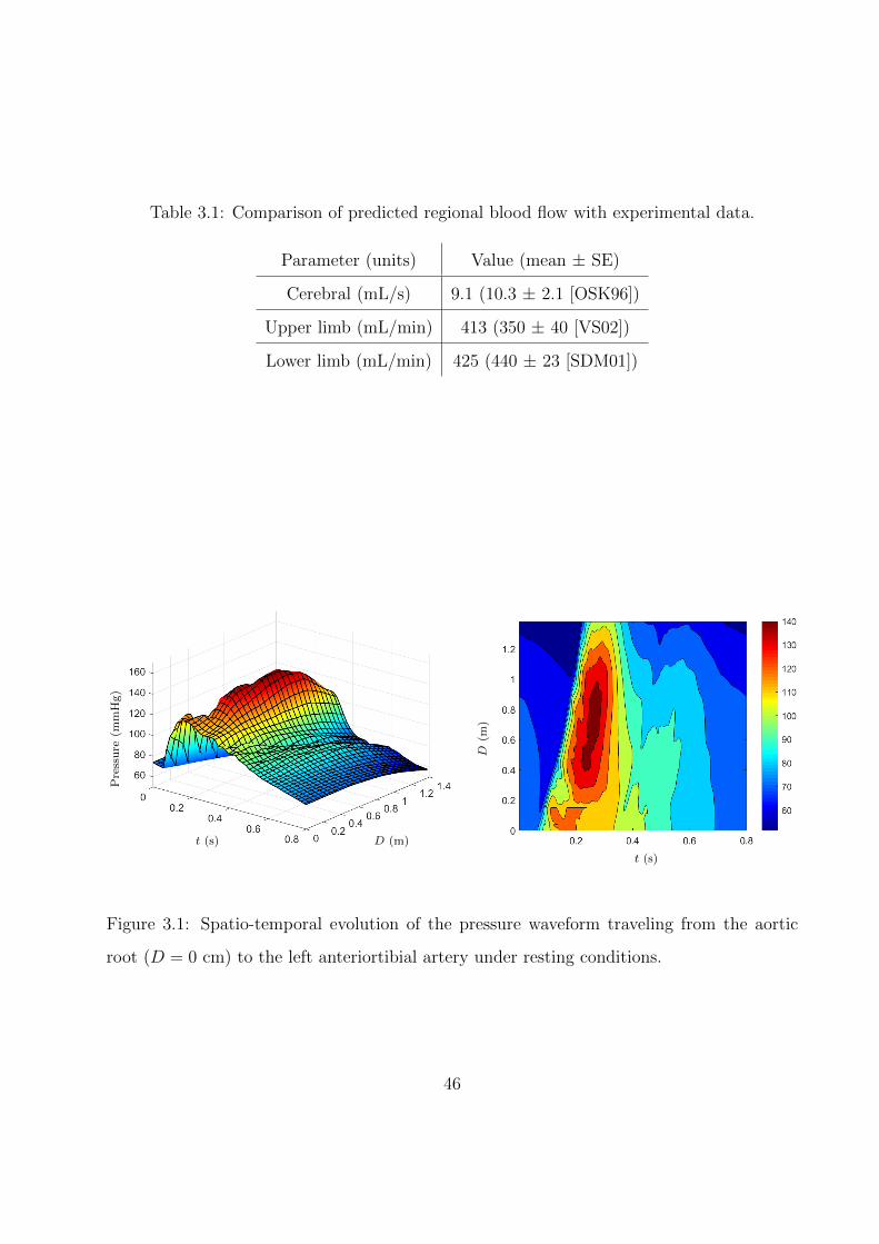
Table 3.1: Comparison of predicted regional blood flow with experimental data.

Parameter (units) Value (mean ± SE)

Cerebral (mL/s) 9.1 (10.3 ± 2.1 [OSK96])

Upper limb (mL/min) 413 (350 ± 40 [VS02])

Lower limb (mL/min) 425 (440 ± 23 [SDM01])

Pre

ssu

re(m

mH

g)

t (s) D (m)

t (s)

D(m

)

Figure 3.1: Spatio-temporal evolution of the pressure waveform traveling from the aortic

root (D = 0 cm) to the left anteriortibial artery under resting conditions.

46

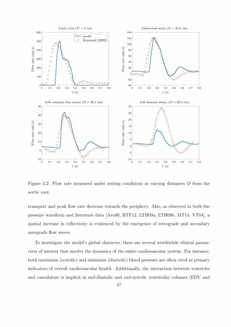
0 0.1 0.2 0.3 0.4 0.5 0.6 0.7 0.8

0

100

200

300

400

500

600

--------------------------

Flo

wra

te(m

L/s)

t (s)

Aortic root (D = 0 cm)

model

Reymond (2009)

0 0.1 0.2 0.3 0.4 0.5 0.6 0.7 0.8

-40

-20

0

20

40

60

80

100

120

140

Flo

wra

te(m

L/s)

t (s)

Abdominal aorta (D = 25.5 cm)

0 0.1 0.2 0.3 0.4 0.5 0.6 0.7 0.8

-10

0

10

20

30

40

50

Flo

wra

te(m

L/s)

t (s)

Left common iliac artery (D = 36.1 cm)

0 0.1 0.2 0.3 0.4 0.5 0.6 0.7 0.8

-10

-5

0

5

10

15

20

25

30

Flo

wra

te(m

L/s)

t (s)

Left femoral artery (D = 50.5 cm)

Figure 3.2: Flow rate measured under resting conditions at varying distances D from the

aortic root.

transport and peak flow rate decrease towards the periphery. Also, as observed in both the

pressure waveform and literature data [Avo80, BTF12, LTH09a, LTH09b, MT14, VT04], a

spatial increase in reflectivity is evidenced by the emergence of retrograde and secondary

antegrade flow waves.

To investigate the model’s global character, there are several worthwhile clinical param-

eters of interest that involve the dynamics of the entire cardiovascular system. For instance,

both maximum (systolic) and minimum (diastolic) blood pressure are often cited as primary

indicators of overall cardiovascular health. Additionally, the interaction between ventricles

and vasculature is implicit in end-diastolic and end-systolic ventricular volumes (EDV and

47

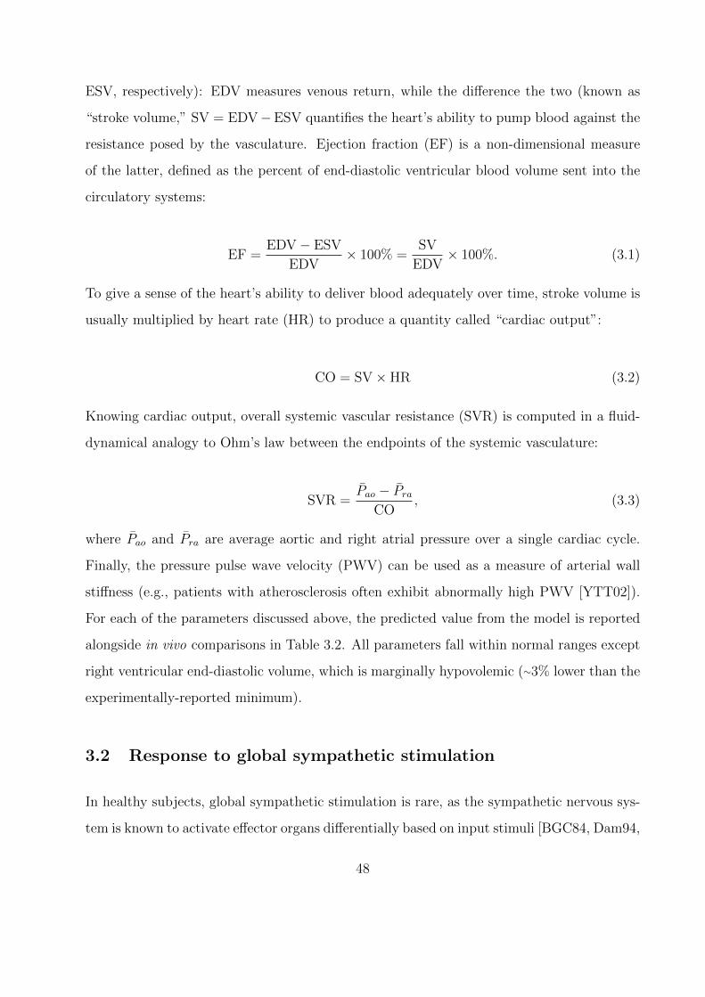
ESV, respectively): EDV measures venous return, while the difference the two (known as

“stroke volume,” SV = EDV−ESV quantifies the heart’s ability to pump blood against the

resistance posed by the vasculature. Ejection fraction (EF) is a non-dimensional measure

of the latter, defined as the percent of end-diastolic ventricular blood volume sent into the

circulatory systems:

EF =EDV− ESV

EDV× 100% =

SV

EDV× 100%. (3.1)

To give a sense of the heart’s ability to deliver blood adequately over time, stroke volume is

usually multiplied by heart rate (HR) to produce a quantity called “cardiac output”:

CO = SV× HR (3.2)

Knowing cardiac output, overall systemic vascular resistance (SVR) is computed in a fluid-

dynamical analogy to Ohm’s law between the endpoints of the systemic vasculature:

SVR =Pao − Pra

CO, (3.3)

where Pao and Pra are average aortic and right atrial pressure over a single cardiac cycle.

Finally, the pressure pulse wave velocity (PWV) can be used as a measure of arterial wall

stiffness (e.g., patients with atherosclerosis often exhibit abnormally high PWV [YTT02]).

For each of the parameters discussed above, the predicted value from the model is reported

alongside in vivo comparisons in Table 3.2. All parameters fall within normal ranges except

right ventricular end-diastolic volume, which is marginally hypovolemic (∼3% lower than the

experimentally-reported minimum).

3.2 Response to global sympathetic stimulation

In healthy subjects, global sympathetic stimulation is rare, as the sympathetic nervous sys-

tem is known to activate effector organs differentially based on input stimuli [BGC84, Dam94,

48

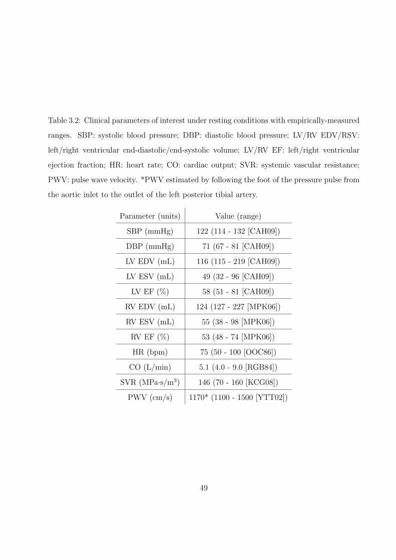
Table 3.2: Clinical parameters of interest under resting conditions with empirically-measured

ranges. SBP: systolic blood pressure; DBP: diastolic blood pressure; LV/RV EDV/RSV:

left/right ventricular end-diastolic/end-systolic volume; LV/RV EF: left/right ventricular

ejection fraction; HR: heart rate; CO: cardiac output; SVR: systemic vascular resistance;

PWV: pulse wave velocity. *PWV estimated by following the foot of the pressure pulse from

the aortic inlet to the outlet of the left posterior tibial artery.

Parameter (units) Value (range)

SBP (mmHg) 122 (114 - 132 [CAH09])

DBP (mmHg) 71 (67 - 81 [CAH09])

LV EDV (mL) 116 (115 - 219 [CAH09])

LV ESV (mL) 49 (32 - 96 [CAH09])

LV EF (%) 58 (51 - 81 [CAH09])

RV EDV (mL) 124 (127 - 227 [MPK06])

RV ESV (mL) 55 (38 - 98 [MPK06])

RV EF (%) 53 (48 - 74 [MPK06])

HR (bpm) 75 (50 - 100 [OOC86])

CO (L/min) 5.1 (4.0 - 9.0 [RGB84])

SVR (MPa·s/m3) 146 (70 - 160 [KCG08])

PWV (cm/s) 1170* (1100 - 1500 [YTT02])

49

FRH11, GJP95, GTA82, JM92, MFH10, Mor01]. However, chronically heightened levels of

sympathetic nervous activity, possibly through a feedback loop of neurotransmitter imbal-

ances [BAP01, BHP69, YML84] and over-active renin-angiontensin and/or sympathoadrenal

systems [Man03], leads to ‘neurogenic’ hypertension. To model this pathological state, the

cardiovascular system was subjected to varying levels of sustained, concurrent sympathetic

stimulation and parasympathetic inhibition (i.e., the values of ns and np in Eq. (2.48) were

set according to a constant, arbitrary pressure, rather than the baroreflex pressure).

The effects of this stimulation on various hemodynamic parameters are displayed in Fig.

3.3. According to established physiological guidelines [CBB03], the systolic and diastolic

limits for hypertension not constituting a medical emergency are 179 and 109 mmHg, respec-

tively. As seen in the figure, these limits correspond to a sympathetic activation of roughly

0.6; this boundary is demarcated by the dashed lines on each plot. Increased sympathetic ac-

tivity results not only in the aforementioned hypertension, but also in tachycardia (elevated

heart rate), as expected from other baroreflex modeling efforts [Dan98, BTF12]. However,

the asymmetric activation function developed in this study permits a higher maximum heart

rate, reaching approximately 180 beats per minute. Though this test was intended to model

hypertension, this maximum is in line with experimental observations during maximal exer-

cise in healthy subjects [HES70, CST87].

Interestingly, Fig. 3.3 also shows that cardiac output exhibits nonlinearity in its re-

sponse to autonomic activity. Prior to the limit for hypertensive emergencies, cardiac out-

put increases, indicating that the induced tachycardia and positive inotropy (as measured

by increasing maximum ventricular elastance) overcomes the reduction in stroke volume

produced by a combination of shorter systolic duration and increased systemic vascular re-

sistance. Indeed, the increase in elastance supports experimental observations of cardiac

hypertrophy (abnormal muscle growth) and wall thickening in response to the augmented

afterload (i.e., SVR) exhibited by hypertensive subjects [MH03]. Furthermore, as displayed

in Table 3.3, the observed elevations in cardiac output and systemic vascular resistance

exhibit close agreement with experimental measurements of patients with hypertension in-

duced by pheochromocytoma (a tumor in the adrenal glands that secretes high levels of

50

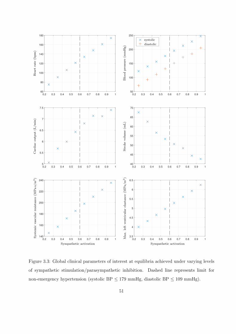
0.2 0.3 0.4 0.5 0.6 0.7 0.8 0.9 1

60

80

100

120

140

160

180H

eart

rate

(bp

m)

0.2 0.3 0.4 0.5 0.6 0.7 0.8 0.9 150

100

150

200

250

systolic----

diastolic

Blo

od

pre

ssu

re(m

mH

g)

systolic

diastolic

0.2 0.3 0.4 0.5 0.6 0.7 0.8 0.9 1

5

5.5

6

6.5

7

7.5

Card

iac

ou

tpu

t(L

/m

in)

0.2 0.3 0.4 0.5 0.6 0.7 0.8 0.9 1

40

45

50

55

60

65

70

Str

oke

volu

me

(mL

)

0.2 0.3 0.4 0.5 0.6 0.7 0.8 0.9 1

140

160

180

200

220

240

Syst

emic

vasc

ula

rre

sist

an

ce(M

Pa·s

/m

3)

Sympathetic activation

0.2 0.3 0.4 0.5 0.6 0.7 0.8 0.9 1

3.5

4

4.5

5

5.5

6

6.5

Max.

left

ven

tric

ula

rel

ast

an

ce(M

Pa/m

3)

Sympathetic activation

Figure 3.3: Global clinical parameters of interest at equilibria achieved under varying levels

of sympathetic stimulation/parasympathetic inhibition. Dashed line represents limit for

non-emergency hypertension (systolic BP ≤ 179 mmHg, diastolic BP ≤ 109 mmHg).

51

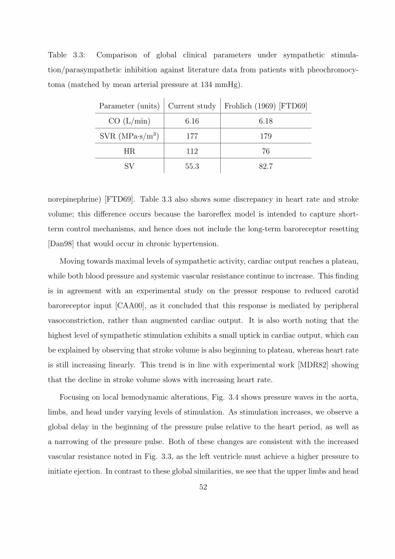
Table 3.3: Comparison of global clinical parameters under sympathetic stimula-

tion/parasympathetic inhibition against literature data from patients with pheochromocy-

toma (matched by mean arterial pressure at 134 mmHg).

Parameter (units) Current study Frohlich (1969) [FTD69]

CO (L/min) 6.16 6.18

SVR (MPa·s/m3) 177 179

HR 112 76

SV 55.3 82.7

norepinephrine) [FTD69]. Table 3.3 also shows some discrepancy in heart rate and stroke

volume; this difference occurs because the baroreflex model is intended to capture short-

term control mechanisms, and hence does not include the long-term baroreceptor resetting

[Dan98] that would occur in chronic hypertension.

Moving towards maximal levels of sympathetic activity, cardiac output reaches a plateau,

while both blood pressure and systemic vascular resistance continue to increase. This finding

is in agreement with an experimental study on the pressor response to reduced carotid

baroreceptor input [CAA00], as it concluded that this response is mediated by peripheral

vasoconstriction, rather than augmented cardiac output. It is also worth noting that the

highest level of sympathetic stimulation exhibits a small uptick in cardiac output, which can

be explained by observing that stroke volume is also beginning to plateau, whereas heart rate

is still increasing linearly. This trend is in line with experimental work [MDR82] showing

that the decline in stroke volume slows with increasing heart rate.

Focusing on local hemodynamic alterations, Fig. 3.4 shows pressure waves in the aorta,

limbs, and head under varying levels of stimulation. As stimulation increases, we observe a

global delay in the beginning of the pressure pulse relative to the heart period, as well as

a narrowing of the pressure pulse. Both of these changes are consistent with the increased

vascular resistance noted in Fig. 3.3, as the left ventricle must achieve a higher pressure to

initiate ejection. In contrast to these global similarities, we see that the upper limbs and head

52

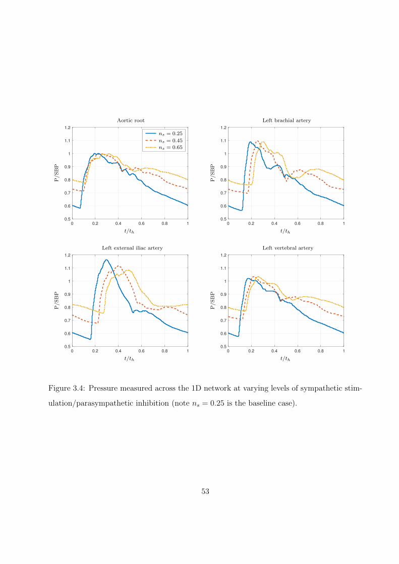
0 0.2 0.4 0.6 0.8 1

0.5

0.6

0.7

0.8

0.9

1

1.1

1.2

aaaaaaaaa

P/S

BP

t/th

Aortic root

ns = 0.25

ns = 0.45

ns = 0.65

0 0.2 0.4 0.6 0.8 1

0.5

0.6

0.7

0.8

0.9

1

1.1

1.2

P/S

BP

t/th

Left brachial artery

0 0.2 0.4 0.6 0.8 1

0.5

0.6

0.7

0.8

0.9

1

1.1

1.2

P/S

BP

t/th

Left external iliac artery

0 0.2 0.4 0.6 0.8 1

0.5

0.6

0.7

0.8

0.9

1

1.1

1.2

P/S

BP

t/th

Left vertebral artery

Figure 3.4: Pressure measured across the 1D network at varying levels of sympathetic stim-

ulation/parasympathetic inhibition (note ns = 0.25 is the baseline case).

53

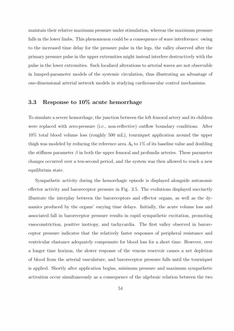
maintain their relative maximum pressure under stimulation, whereas the maximum pressure

falls in the lower limbs. This phenomenon could be a consequence of wave interference: owing

to the increased time delay for the pressure pulse in the legs, the valley observed after the

primary pressure pulse in the upper extremities might instead interfere destructively with the

pulse in the lower extremities. Such localized alterations to arterial waves are not observable

in lumped-parameter models of the systemic circulation, thus illustrating an advantage of

one-dimensional arterial network models in studying cardiovascular control mechanisms.

3.3 Response to 10% acute hemorrhage

To simulate a severe hemorrhage, the junction between the left femoral artery and its children

were replaced with zero-pressure (i.e., non-reflective) outflow boundary conditions. After

10% total blood volume loss (roughly 500 mL), tourniquet application around the upper

thigh was modeled by reducing the reference area A0 to 1% of its baseline value and doubling

the stiffness parameter β in both the upper femoral and profundis arteries. These parameter

changes occurred over a ten-second period, and the system was then allowed to reach a new

equilibrium state.

Sympathetic activity during the hemorrhagic episode is displayed alongside autonomic

effector activity and baroreceptor pressure in Fig. 3.5. The evolutions displayed succinctly

illustrate the interplay between the baroreceptors and effector organs, as well as the dy-

namics produced by the organs’ varying time delays. Initially, the acute volume loss and

associated fall in baroreceptor pressure results in rapid sympathetic excitation, promoting

vasoconstriction, positive inotropy, and tachycardia. The first valley observed in barore-

ceptor pressure indicates that the relatively faster responses of peripheral resistance and

ventricular elastance adequately compensate for blood loss for a short time. However, over

a longer time horizon, the slower response of the venous reservoir causes a net depletion

of blood from the arterial vasculature, and baroreceptor pressure falls until the tourniquet

is applied. Shortly after application begins, minimum pressure and maximum sympathetic

activation occur simultaneously as a consequence of the algebraic relation between the two

54

0 10 20 30 40 50 60 70 80 90

0.2

0.3

0.4

0.5

0.6

0.7

0.8

Sym

path

etic

act

ivati

on

0 10 20 30 40 50 60 70 80 90

0.7

0.75

0.8

0.85

0.9

0.95

1

Pbaro/ψ

0 10 20 30 40 50 60 70 80 90

0.8

1

1.2

1.4

1.6

1.8

2

aaaaaaaaaaaR/R0

C/C0

Elv/Elv,0Vun/Vun,0

Eff

ecto

rre

spon

se

t (s)

0 10 20 30 40 50 60 70 80 90

70

80

90

100

110

120

130

140

150

160

Hea

rtra

te(b

pm

)

t (s)

Figure 3.5: Sympathetic activation, baroreceptor pressure, and effector organ responses dur-

ing acute 10% hemorrhage. Pressure and effector responses (excluding heart rate) normalized

by basal values. Region between dashed lines indicates period of tourniquet application.

55

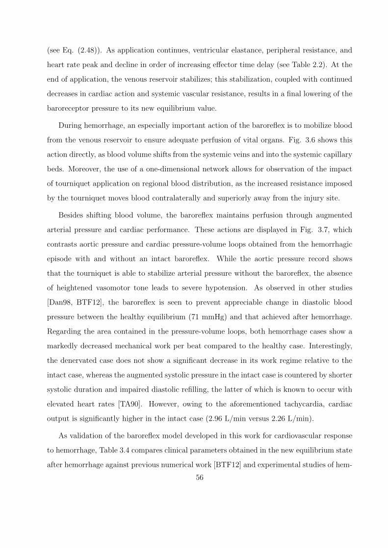
(see Eq. (2.48)). As application continues, ventricular elastance, peripheral resistance, and

heart rate peak and decline in order of increasing effector time delay (see Table 2.2). At the

end of application, the venous reservoir stabilizes; this stabilization, coupled with continued

decreases in cardiac action and systemic vascular resistance, results in a final lowering of the

baroreceptor pressure to its new equilibrium value.

During hemorrhage, an especially important action of the baroreflex is to mobilize blood

from the venous reservoir to ensure adequate perfusion of vital organs. Fig. 3.6 shows this

action directly, as blood volume shifts from the systemic veins and into the systemic capillary

beds. Moreover, the use of a one-dimensional network allows for observation of the impact

of tourniquet application on regional blood distribution, as the increased resistance imposed

by the tourniquet moves blood contralaterally and superiorly away from the injury site.

Besides shifting blood volume, the baroreflex maintains perfusion through augmented

arterial pressure and cardiac performance. These actions are displayed in Fig. 3.7, which

contrasts aortic pressure and cardiac pressure-volume loops obtained from the hemorrhagic

episode with and without an intact baroreflex. While the aortic pressure record shows

that the tourniquet is able to stabilize arterial pressure without the baroreflex, the absence

of heightened vasomotor tone leads to severe hypotension. As observed in other studies

[Dan98, BTF12], the baroreflex is seen to prevent appreciable change in diastolic blood

pressure between the healthy equilibrium (71 mmHg) and that achieved after hemorrhage.

Regarding the area contained in the pressure-volume loops, both hemorrhage cases show a

markedly decreased mechanical work per beat compared to the healthy case. Interestingly,

the denervated case does not show a significant decrease in its work regime relative to the

intact case, whereas the augmented systolic pressure in the intact case is countered by shorter

systolic duration and impaired diastolic refilling, the latter of which is known to occur with

elevated heart rates [TA90]. However, owing to the aforementioned tachycardia, cardiac

output is significantly higher in the intact case (2.96 L/min versus 2.26 L/min).

As validation of the baroreflex model developed in this work for cardiovascular response

to hemorrhage, Table 3.4 compares clinical parameters obtained in the new equilibrium state

after hemorrhage against previous numerical work [BTF12] and experimental studies of hem-

56

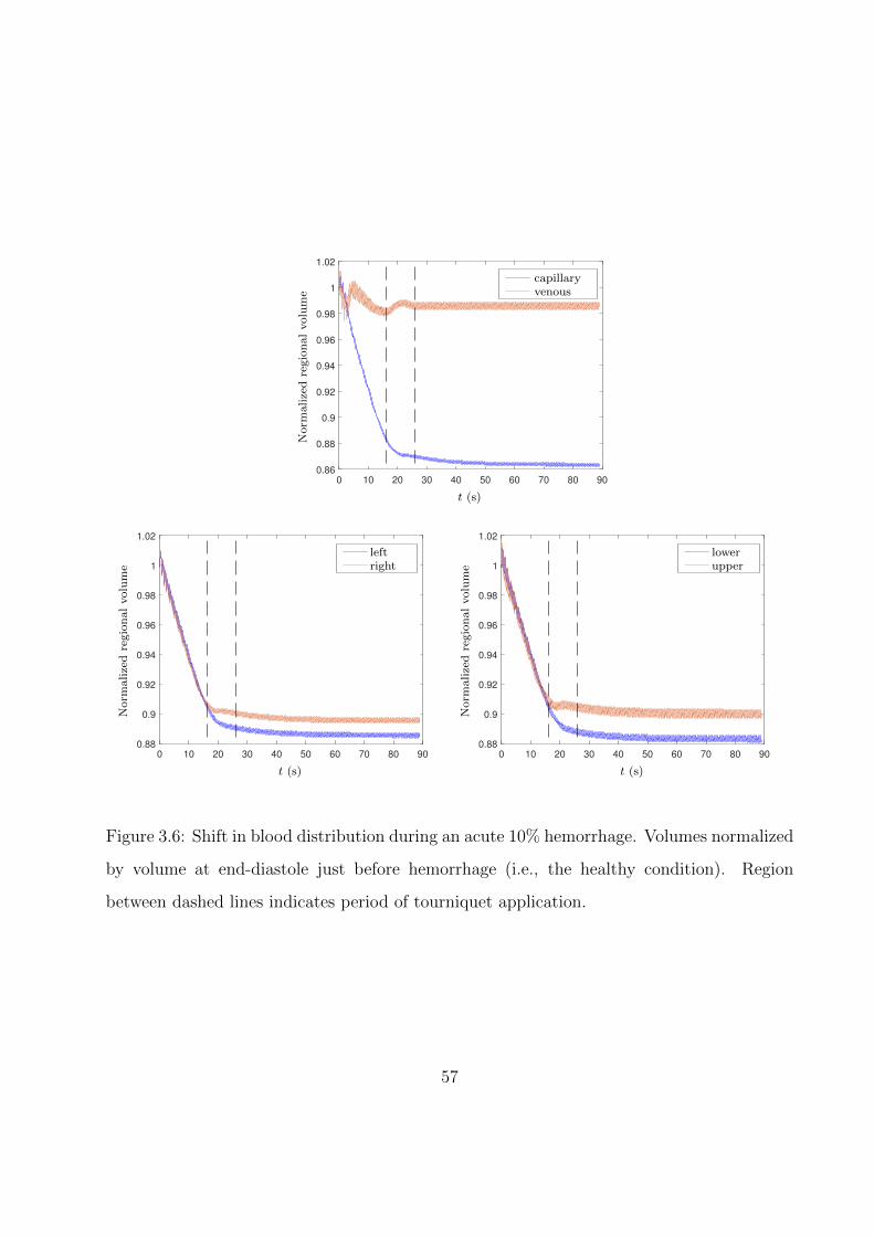
0 10 20 30 40 50 60 70 80 90

0.86

0.88

0.9

0.92

0.94

0.96

0.98

1

1.02

aaaaaaaaaacapillaryvenous

Norm

alize

dre

gio

nal

volu

me

t (s)

0 10 20 30 40 50 60 70 80 90

0.88

0.9

0.92

0.94

0.96

0.98

1

1.02

aaaaaaaleftright

Norm

alize

dre

gio

nal

volu

me

t (s)

0 10 20 30 40 50 60 70 80 90

0.88

0.9

0.92

0.94

0.96

0.98

1

1.02

aaaaaaalowerupper

Norm

alize

dre

gio

nal

volu

me

t (s)

Figure 3.6: Shift in blood distribution during an acute 10% hemorrhage. Volumes normalized

by volume at end-diastole just before hemorrhage (i.e., the healthy condition). Region

between dashed lines indicates period of tourniquet application.

57

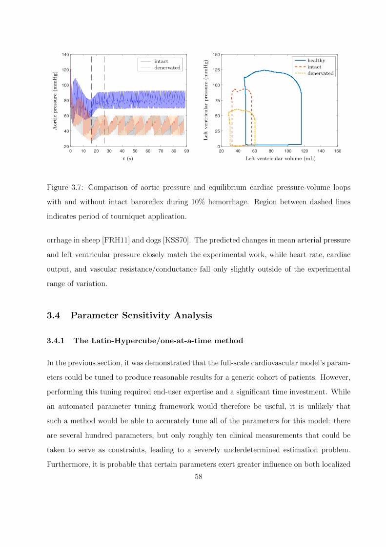
0 10 20 30 40 50 60 70 80 90

20

40

60

80

100

120

140

aaaaaaaaaaaintactdenervated

Aort

icp

ress

ure

(mm

Hg)

t (s)

20 40 60 80 100 120 140 160

0

25

50

75

100

125

150

aaaaaaaaaa

Lef

tven

tric

ula

rp

ress

ure

(mm

Hg)

Left ventricular volume (mL)

healthyintactdenervated

Figure 3.7: Comparison of aortic pressure and equilibrium cardiac pressure-volume loops

with and without intact baroreflex during 10% hemorrhage. Region between dashed lines

indicates period of tourniquet application.

orrhage in sheep [FRH11] and dogs [KSS70]. The predicted changes in mean arterial pressure

and left ventricular pressure closely match the experimental work, while heart rate, cardiac

output, and vascular resistance/conductance fall only slightly outside of the experimental

range of variation.

3.4 Parameter Sensitivity Analysis

3.4.1 The Latin-Hypercube/one-at-a-time method

In the previous section, it was demonstrated that the full-scale cardiovascular model’s param-

eters could be tuned to produce reasonable results for a generic cohort of patients. However,

performing this tuning required end-user expertise and a significant time investment. While

an automated parameter tuning framework would therefore be useful, it is unlikely that

such a method would be able to accurately tune all of the parameters for this model: there

are several hundred parameters, but only roughly ten clinical measurements that could be

taken to serve as constraints, leading to a severely underdetermined estimation problem.

Furthermore, it is probable that certain parameters exert greater influence on both localized

58

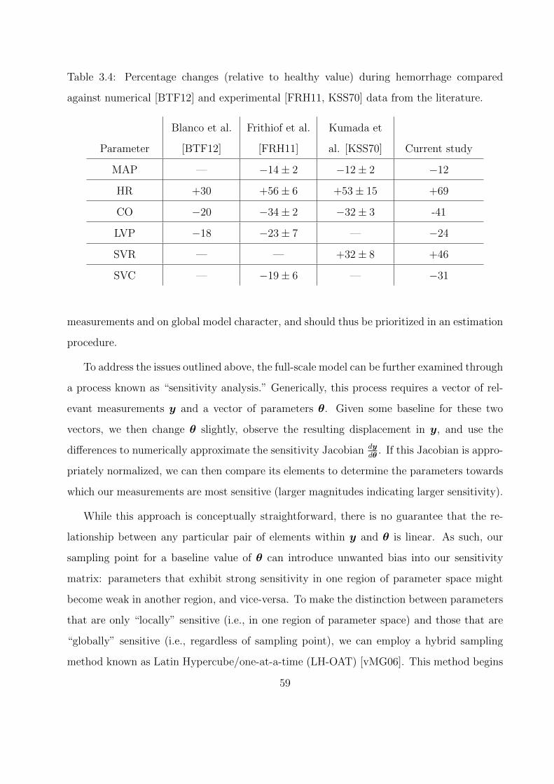
Table 3.4: Percentage changes (relative to healthy value) during hemorrhage compared

against numerical [BTF12] and experimental [FRH11, KSS70] data from the literature.

Parameter

Blanco et al.

[BTF12]

Frithiof et al.

[FRH11]

Kumada et

al. [KSS70] Current study

MAP — −14± 2 −12± 2 −12

HR +30 +56± 6 +53± 15 +69

CO −20 −34± 2 −32± 3 -41

LVP −18 −23± 7 — −24

SVR — — +32± 8 +46

SVC — −19± 6 — −31

measurements and on global model character, and should thus be prioritized in an estimation

procedure.

To address the issues outlined above, the full-scale model can be further examined through

a process known as “sensitivity analysis.” Generically, this process requires a vector of rel-

evant measurements y and a vector of parameters θ. Given some baseline for these two

vectors, we then change θ slightly, observe the resulting displacement in y, and use the

differences to numerically approximate the sensitivity Jacobian dydθ

. If this Jacobian is appro-

priately normalized, we can then compare its elements to determine the parameters towards

which our measurements are most sensitive (larger magnitudes indicating larger sensitivity).

While this approach is conceptually straightforward, there is no guarantee that the re-

lationship between any particular pair of elements within y and θ is linear. As such, our

sampling point for a baseline value of θ can introduce unwanted bias into our sensitivity

matrix: parameters that exhibit strong sensitivity in one region of parameter space might

become weak in another region, and vice-versa. To make the distinction between parameters

that are only “locally” sensitive (i.e., in one region of parameter space) and those that are

“globally” sensitive (i.e., regardless of sampling point), we can employ a hybrid sampling

method known as Latin Hypercube/one-at-a-time (LH-OAT) [vMG06]. This method begins

59

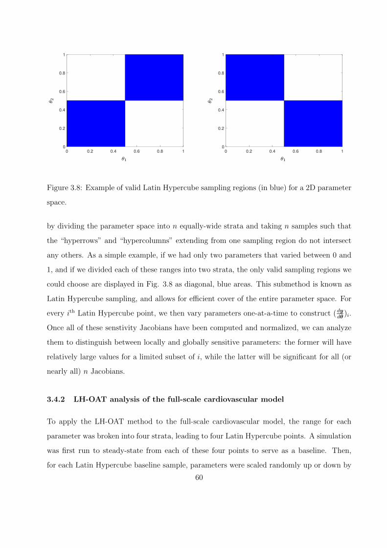
0 0.2 0.4 0.6 0.8 1

0

0.2

0.4

0.6

0.8

1

θ 2

θ1

0 0.2 0.4 0.6 0.8 1

0

0.2

0.4

0.6

0.8

1

θ 2

θ1

Figure 3.8: Example of valid Latin Hypercube sampling regions (in blue) for a 2D parameter

space.

by dividing the parameter space into n equally-wide strata and taking n samples such that

the “hyperrows” and “hypercolumns” extending from one sampling region do not intersect

any others. As a simple example, if we had only two parameters that varied between 0 and

1, and if we divided each of these ranges into two strata, the only valid sampling regions we

could choose are displayed in Fig. 3.8 as diagonal, blue areas. This submethod is known as

Latin Hypercube sampling, and allows for efficient cover of the entire parameter space. For

every ith Latin Hypercube point, we then vary parameters one-at-a-time to construct (dydθ

)i.

Once all of these senstivity Jacobians have been computed and normalized, we can analyze

them to distinguish between locally and globally sensitive parameters: the former will have

relatively large values for a limited subset of i, while the latter will be significant for all (or

nearly all) n Jacobians.

3.4.2 LH-OAT analysis of the full-scale cardiovascular model

To apply the LH-OAT method to the full-scale cardiovascular model, the range for each

parameter was broken into four strata, leading to four Latin Hypercube points. A simulation

was first run to steady-state from each of these four points to serve as a baseline. Then,

for each Latin Hypercube baseline sample, parameters were scaled randomly up or down by

60

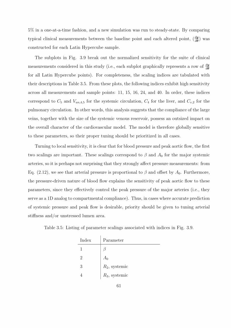
5% in a one-at-a-time fashion, and a new simulation was run to steady-state. By comparing

typical clinical measurements between the baseline point and each altered point, (dydθ

) was

constructed for each Latin Hypercube sample.

The subplots in Fig. 3.9 break out the normalized sensitivity for the suite of clinical

measurements considered in this study (i.e., each subplot graphically represents a row of dydθ

for all Latin Hypercube points). For completeness, the scaling indices are tabulated with

their descriptions in Table 3.5. From these plots, the following indices exhibit high sensitivity

across all measurements and sample points: 11, 15, 16, 24, and 40. In order, these indices

correspond to C5 and Vun,4,5 for the systemic circulation, C4 for the liver, and Cv,2 for the

pulmonary circulation. In other words, this analysis suggests that the compliance of the large

veins, together with the size of the systemic venous reservoir, possess an outsized impact on

the overall character of the cardiovascular model. The model is therefore globally sensitive

to these parameters, so their proper tuning should be prioritized in all cases.

Turning to local sensitivity, it is clear that for blood pressure and peak aortic flow, the first

two scalings are important. These scalings correspond to β and A0 for the major systemic

arteries, so it is perhaps not surprising that they strongly affect pressure measurements: from

Eq. (2.12), we see that arterial pressure is proportional to β and offset by A0. Furthermore,

the pressure-driven nature of blood flow explains the sensitivity of peak aortic flow to these

parameters, since they effectively control the peak pressure of the major arteries (i.e., they

serve as a 1D analog to compartmental compliance). Thus, in cases where accurate prediction

of systemic pressure and peak flow is desirable, priority should be given to tuning arterial

stiffness and/or unstressed lumen area.

Table 3.5: Listing of parameter scalings associated with indices in Fig. 3.9.

Index Parameter

1 β

2 A0

3 R2, systemic

4 R3, systemic

61

5 R4, systemic

6 R5, systemic

7 C1, systemic

8 C2, systemic

9 C3, systemic

10 C4, systemic

11 C5, systemic

12 Vun,1, systemic

13 Vun,2, systemic

14 Vun,3, systemic

15 Vun,4, systemic

16 Vun,5, systemic

17 R1, liver

18 R2, liver

19 R3, liver

20 R4, liver

21 C1, liver

22 C2, liver

23 C3, liver

24 C4, liver

25 Vun,1, liver

26 Vun,2, liver

27 Vun,3, liver

28 Vun,4, liver

29 L4, liver

30 Rp, lungs

31 Ra,1, lungs

32 Ra,2, lungs

33 Ra,3, lungs

62

34 Rv,1, lungs

35 Rv,2, lungs

36 Ca,1, lungs

37 Ca,2, lungs

38 Ca,3, lungs

39 Cv,1, lungs

40 Cv,2, lungs

41 Vun,1, lungs

42 Vun,2, lungs

43 Vun,3, lungs

44 Vun,4, lungs

45 Vun,5, lungs

46 La, lungs

47 Lv, lungs

48 lower/upper body flow split

49 venous resistance fraction

50 venous inductance fraction

51 venous capacitance fraction

52 venous Vun fraction

53 m1, elastance function

54 m2, elastance function

55 τ1, elastance function

56 τ2, elastance function

57 Emax,lv, elastance function

58 Emax,lv, elastance function

59 Vun,lv, heart

60 Vun,rv, heart

61 Vun,la, heart

62 Rla, heart

63

63 Lla, heart

64 Ela, heart

65 Vun,ra, heart

66 Rra, heart

67 Lra, heart

68 Era, heart

69 Lrv, heart

70 L5, systemic

64

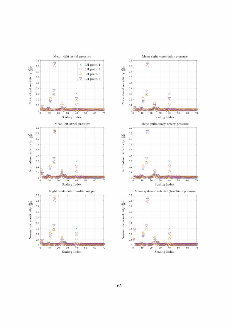
0 10 20 30 40 50 60 70

0

0.1

0.2

0.3

0.4

0.5

0.6

0.7

0.8

0.9

---------------

Norm

alize

dse

nsi

tivit

ydy∗

dθ∗

Scaling Index

Mean right atrial pressure

LH point 1

LH point 2

LH point 3

LH point 4

0 10 20 30 40 50 60 70

0

0.1

0.2

0.3

0.4

0.5

0.6

0.7

0.8

0.9

Norm

alize

dse

nsi

tivit

ydy∗

dθ∗

Scaling Index

Mean right ventricular pressure

0 10 20 30 40 50 60 70

0

0.1

0.2

0.3

0.4

0.5

0.6

0.7

0.8

0.9

Norm

alize

dse

nsi

tivit

ydy∗

dθ∗

Scaling Index

Mean left atrial pressure

0 10 20 30 40 50 60 70

0

0.1

0.2

0.3

0.4

0.5

0.6

0.7

0.8

0.9

Norm

alize

dse

nsi

tivit

ydy∗

dθ∗

Scaling Index

Mean pulmonary artery pressure

0 10 20 30 40 50 60 70

0

0.1

0.2

0.3

0.4

0.5

0.6

0.7

0.8

0.9

Norm

alize

dse

nsi

tivit

ydy∗

dθ∗

Scaling Index

Right ventricular cardiac output

0 10 20 30 40 50 60 70

0

0.1

0.2

0.3

0.4

0.5

0.6

0.7

0.8

0.9

Norm

alize

dse

nsi

tivit

ydy∗

dθ∗

Scaling Index

Mean systemic arterial (brachial) pressure

65

0 10 20 30 40 50 60 70

0

0.1

0.2

0.3

0.4

0.5

0.6

0.7

0.8

Norm

alize

dse

nsi

tivit

ydy∗

dθ∗

Scaling Index

Left ventricular end-diastolic volume

0 10 20 30 40 50 60 70

0

0.1

0.2

0.3

0.4

0.5

0.6

0.7

0.8

Norm

alize

dse

nsi

tivit

ydy∗

dθ∗

Scaling Index

Right ventricular end-diastolic volume

0 10 20 30 40 50 60 70

0

0.1

0.2

0.3

0.4

0.5

0.6

0.7

0.8

0.9

Norm

alize

dse

nsi

tivit

ydy∗

dθ∗

Scaling Index

Left ventricular cardiac output

0 10 20 30 40 50 60 70

0

0.2

0.4

0.6

0.8

1

Norm

alize

dse

nsi

tivit

ydy∗

dθ∗

Scaling Index

Peak aortic flow rate

0 10 20 30 40 50 60 70

0

0.1

0.2

0.3

0.4

0.5

0.6

0.7

0.8

0.9

Norm

alize

dse

nsi

tivit

ydy∗

dθ∗

Scaling Index

Mean vena caval pressure

Figure 3.9: Normalized LH-OAT parameter sensitivities for various clinical measurement

predictions. Scaling indices are linked to parameters tabulated in Table 3.5.

66

CHAPTER 4

Data Assimilation and Parameter Estimation

As seen from the previous chapter, a complete cardiovascular model requires dozens of model

parameters. Furthermore, these parameters are related in a nonlinear fashion to both model

predictions and one another. As such, adjustment of these parameters in an ad-hoc way is

time-consuming and requires significant end-user expertise. To lower this hurdle, develop-

ment of an algorithm for automated parameter estimation based on clinical data would be

ideal. In this work, an ensemble Kalman Filter (EnKF) is developed for this purpose. In

this chapter, a brief overview of Kalman filtering algorithms is given, followed by further

details for particular filters and alterations to improve filter robustness. The chapter closes

with a simple “toy” problem to demonstrate the effectiveness of the EnKF under decreasing

measurement availability.

4.1 Overview of the Kalman filter framework

The ensemble Kalman filter (EnKF) was originally developed by Evensen [Eve03] to assimi-

late measurement data into high-dimensional, nonlinear meteorological models. However, it

is only one instance of a larger framework for Kalman filtering algorithms [JUD95, TAC14].

To describe this framework, we begin with the governing equations for the true state and

measurements of a discrete-time, possibly nonlinear dynamical system with additive noise:

xn = M(xn−1) +wn−1,

yn = h(xn) + vn.

(4.1)

In Eq. (4.1), we never have access to the true state, nor do we know the exact noise

67

levels. Therefore, we will distinguish our model equations with a change in font to indicate

multivariate random variables:

Xn = M(Xn−1) +Wn−1,

Yn = h(Xn) + Vn.

(4.2)

To proceed, we constrain the distributions of the initial state, process noise, and mea-

surement noise to be Gaussian with independent covariances. Furthermore, we require the

noise distributions to be zero mean. More concisely:

X0 ∼ N (x0,P0),

Wn ∼ N (0,Wn),

Vn ∼ N (0,Vn),

(4.3)

where N (µ,C) symbolizes a Gaussian distribution with mean µ and covariance matrix C.

Since the noise is assumed to be zero-mean, we can propogate the mean model state x and

its associated measurement y forward in time using Eq. (4.2):

x−n = M(xn−1),

yn = h(x−n ),

(4.4)

where the “-” superscript indicates that the true measurement has not been incorporated

into this prediction (often called the forecast step). At this point, we would like to improve

our forecast using the true measurement. One intuitive way to do so is to use some linear

combination of the difference between the model’s predicted measurement yn and the true

measurement yn (usually called the innovation). Specifically, we would like to write:

yn = yn − yn,

x+n = x−n +Knyn,

(4.5)

68

where Kn is the Kalman gain matrix and the “+” superscript denotes the assimilation of

measurement data into the prediction (known as the analysis step). Instead of defining Kn

arbitrarily, we can optimize it using the error in the state vector (note omission of the time

step index for brevity):

x = x− x. (4.6)

With the state error defined, we can write the error covariance matrix for the analysis

step in terms of the Kalman gain, the innovation, and the forecast step:

x+ = x− −Ky,

P+ = E[x+x+T ]

= E[x−x−T − x−yTKT −Kyx−T +KyyTKT ]

= P− − cov(x−, y)KT −Kcov(y, x−) +Kcov(y, y)KT ,

(4.7)

where E[·] is the expected value and cov(a, b) is the cross-covariance matrix of a and b.

For convenience, we define Q ≡ cov(x−, y) and R ≡ cov(y, y). Then, under the Gaussian

assumption, we can obtain an expression for the Kalman gain by minimizing the trace of the

analysis error with respect to K (i.e., by seeking to minimize the error in each state variable

after analysis):

∂[tr(P+)]

∂K= 0

−2Q + 2KR = 0

K = QR−1.

(4.8)

Finally, we can also compute the analysis error covariance by combining the final lines of

Eqs. (4.7) and (4.8):

P+ = P− −KQ. (4.9)

69

To summarize, all Kalman filtering algorithms share the following steps:

1. Forecast (advance model in time):

x−n = M(xn−1),

yn = h(x−n ).

(4.10)

2. Compute the Kalman gain (determine strength of model correction):

Kn = QnRn−1. (4.11)

3. Analysis (correct model using measurement):

x+n = x−n +Knyn,

P+n = P−n −KnQn.

(4.12)

Within the steps above, the primary source of differentiation between Kalman methods is

in the computation of the covariance/cross-covariance matrices Qn, Rn, and P−n . In the

following two sections, we will see that the classical Kalman filter is able to compute these

matrices analytically for linear systems. By contrast, to work with nonlinear systems, the

EnKF will develop approximations by using the statistics of an ensemble of simulations.

4.2 The classical Kalman filter

To develop the framework in Sec. 4.1, we assumed:

1. Both process noise w and measurement noise v are additive.

2. The initial state distributionX0, process noise distributionW , and measurement noise

distribution V are Gaussian with independent covariances.

3. The process and measurement noise distributions have zero mean.

70

In the standard Kalman filter [Kal60], we additionally assume that the dynamics and mea-

surement operator are both linear, so the forecast step given in Eq. (4.10) becomes:

x−n = Mx+n−1,

yn = Hx−n .(4.13)

Next, by making frequent use of the independent covariances listed above, we compute the

Kalman gain from Eq. (4.11):

yn = yn − yn = Hxn + vn −Hxn = Hxn + vn,

Qn = E[x−n yTn ] = E[x−n (x−Tn HT + vTn )] = cov(x−n , x

−n )

= P−nHT ,

Rn = E[ynyTn ] = HP−nH

T + Vn,

P−n ≈ E[(Xn − x−n )(Xn − x−n )T ]

= E[(MXn−1 +Wn −Mx+n−1)(MXn−1 +Wn −Mx+

n−1)T ]

= ME[(Xn−1 − x+n−1)(Xn−1 − x+

n−1)T ]MT + Wn

= MP+n−1M

T + Wn,

Kn = QnRn−1 = P−nH

T (HP−nHT + Vn)−1.

(4.14)

Finally, the analysis step:

x+n = x−n +Knyn,

P+n = P−n −KnQn = (I−KnH)P−n .

(4.15)

Thus, we see that the classical Kalman filter is able to analytically evaluate all of the

covariance and cross-covariance matrices necessary for its operation. However, there are

some important points to observe about Eqs. (4.14) and (4.15), specifically with regard to

the state covariance matrix Pn. First, we assume that the forecast state covariance matrix

P−n is an adequate approximation to the forecast error covariance (hence the approximation

sign in the first line of P−n ’s development). Second, P−n is defined recursively from P+n−1. For

71

these two reasons, the specification of the initial state covariance P0 plays a significant part

in the initial performance of our model, though its role may diminish as data is assimilated

through P+n . Finally, while it is possible for P+

n−1 to approach zero at the analysis step,

the following forecast step P−n is always bounded from below by the process noise covariance

Wn. As we will see in the next section, the state covariance in the EnKF does not inherently

possess such a lower bound, and thus requires artificial covariance inflation for robustness.

4.3 The ensemble Kalman filter (EnKF)

4.3.1 Evensen’s original method

In the case that the dynamics and measurement operator are nonlinear, then the matrices

P−n , Qn, and Rn can no longer be evaluated analytically. Instead, the ensemble Kalman

filter (EnKF) makes approximations to these matrices by using statistics from an ensemble

of L models. We begin with the usual forecast step for every ith ensemble member:

x−i,n = M(x+i,n−1),

yi,n = h(x−i,n),for i = 1, 2, . . . , L. (4.16)

Following the ensemble forecast, we approximate the mean of the system state and measure-

ment distributions using their ensemble means:

x−n ≈ x−n ≡1

L− 1

L∑i=1

x−i,n,

yn ≈ yn ≡1

L− 1

L∑i=1

yi,n.

(4.17)

The necessary covariance/cross-covariance matrices are approximated in a similar fashion:

72

P−n = E[(Xn − xn)(Xn − xn)T ] ≈ 1

L− 1

L∑i=1

(x−i,n − x−n )(x−i,n − x−n )T ,

Qn = E[x−n yTn ] ≈ 1

L− 1

L∑i=1

(x−i,n − xn)(yi,n − yn)T ,

Rn = E[ynyTn ] ≈ 1

L− 1

L∑i=1

(yi,n − yn)(yi,n − yn)T + Vn.

(4.18)

The Kalman gain is then computed normally, and is shared across all ensemble members:

Kn = QnRn−1. (4.19)

Finally, to avoid spurious correlations in the ensemble covariance [BLE98], noise is added to

the innovation of each ensemble member during the analysis step:

x+i,n = x−i,n +Kn(yn + εi − yi,n) for i = 1, 2, . . . , L, (4.20)

where each perturbation εi is taken from Vn.

4.3.2 Covariance inflation

By comparing P−n in Eqs. (4.15) and (4.18), we see that only the former possesses a lower

bound (due to the presence of Wn). Thus, in the original EnKF formulation, it is possible

for the state covariance to approach zero (i.e., xi,n → xn for all i). This phenomenon is

known as covariance collapse or filter divergence [WH12], and results in Kn going to zero,

after which point all measurements are ignored. To avoid this behavior, it is necessary to

artificially inflate the state covariance:

xi,n ← xi,n + αn(xi,n − xn) + βi,n, (4.21)

where αn is a multiplicative inflation factor common to all ensemble members [AA99], and

βi,n is an additive inflation factor drawn for each ensemble member from a random distri-

bution [MH00]. For high-dimensional systems, additive inflation is generally undesirable, as

73

it requires individual tuning for each element of the state vector. For multiplicative infla-

tion, there are several different inflation techniques; the one employed in this work is the

relaxation-to-prior-spread (RTPS) method developed by Whitaker and Hamill [WH12]. In

this method, we first compute the standard deviation for the ensemble after forecast and

analysis:

σ−n =

√√√√ 1

L− 1

L∑i=1

(x−i,n − x−n ),

σ+n =

√√√√ 1

L− 1

L∑i=1

(x+i,n − x+

n ).

(4.22)

We then use the normalized difference between the two standard deviations to drive each

ensemble member away from the ensemble mean:

x+i,n − x+

n ← (x+i,n − x+

n )

(cσ−n − σ+

n

σ+n

+ 1

)for i = 1, 2, . . . , L, (4.23)

where the constant c (typically between 0.5 and 1) controls the amount of relaxation. Note

that for implementation, it is more convenient to rewrite the above equation as

x+i,n ← x+

i,n + cσ−n − σ+

n

σ+n

(x+i,n − x+

n ). (4.24)

The RTPS scheme was chosen for this work because of its simplicity (it requires only one

tunable parameter) and its robustness: numerical experiments from weather forecast models

(i.e., chaotic systems) show stable model errors that are relatively insensitive to the value of

the inflation parameter [WH12].

74

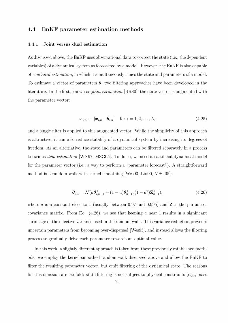
4.4 EnKF parameter estimation methods

4.4.1 Joint versus dual estimation

As discussed above, the EnKF uses observational data to correct the state (i.e., the dependent

variables) of a dynamical system as forecasted by a model. However, the EnKF is also capable

of combined estimation, in which it simultaneously tunes the state and parameters of a model.

To estimate a vector of parameters θ, two filtering approaches have been developed in the

literature. In the first, known as joint estimation [BR80], the state vector is augmented with

the parameter vector:

xi,n ← [xi,n θi,n] for i = 1, 2, . . . , L, (4.25)

and a single filter is applied to this augmented vector. While the simplicity of this approach

is attractive, it can also reduce stability of a dynamical system by increasing its degrees of

freedom. As an alternative, the state and parameters can be filtered separately in a process

known as dual estimation [WN97, MSG05]. To do so, we need an artificial dynamical model

for the parameter vector (i.e., a way to perform a “parameter forecast”). A straightforward

method is a random walk with kernel smoothing [Wes93, Liu00, MSG05]:

θ−i,n = N (aθ+i,n−1 + (1− a)θ+

n−1, (1− a2)Z+n−1), (4.26)

where a is a constant close to 1 (usually between 0.97 and 0.995) and Z is the parameter

covariance matrix. From Eq. (4.26), we see that keeping a near 1 results in a significant

shrinkage of the effective variance used in the random walk. This variance reduction prevents

uncertain parameters from becoming over-dispersed [Wes93], and instead allows the filtering

process to gradually drive each parameter towards an optimal value.

In this work, a slightly different approach is taken from these previously established meth-

ods: we employ the kernel-smoothed random walk discussed above and allow the EnKF to

filter the resulting parameter vector, but omit filtering of the dynamical state. The reasons

for this omission are twofold: state filtering is not subject to physical constraints (e.g., mass

75

conservation), and we would like to study the degree to which a parametrically-optimized

reduced-order model approximates individual patient measurements without artificial alter-

ations to its state.

4.4.2 The complete parameter estimation procedure

Listed below are the complete set of steps used for parameter estimation through the EnKF.

Note that θ has been inserted into the list of arguments for the dynamics M and the mea-

surement h to make their parameter dependence clear.

1. Generate perturbed measurements:

y′n = yn + εi, εi ∼ N (0,Vn) for i = 1, 2, . . . , L. (4.27)

2. Parameter forecast step:

Z+n−1 = var(θ+

n−1),

θ−i,n = N (aθ+i,n−1 + (1− a)θ+

n−1, (1− a2)Z+n−1) for i = 1, 2, . . . , L.

(4.28)

3. State forecast with forecasted parameters:

x−i,n = M(x+i,n−1,θ

−i,n),

yi,n = h(x−i,n,θ−i,n),

for i = 1, 2, . . . , L. (4.29)

4. Compute parameter Kalman gain:

Qθ,n =1

L− 1

L∑i=1

(θ−i,n − θn)(yi,n − yn)T ,

Rθ,n =1

L− 1

L∑i=1

(yi,n − yn)(yi,n − yn)T + Vn,

Kθ,n = Qθ,nR−1θ,n.

(4.30)

5. Parameter analysis step:

θ+i,n = θ−i,n +Kθ,n(y′n − yi,n) for i = 1, 2, . . . , L. (4.31)

76

6. Parameter RTPS covariance inflation:

σ−θ,n =

√√√√ 1

L− 1

L∑i=1

(θ−i,n − θ−n ),

σ+θ,n =

√√√√ 1

L− 1

L∑i=1

(θ+i,n − θ+

n ),

θ+i,n ← θ+

i,n + cσ−θ,n − σ

+θ,n

σ+θ,n

(θ+i,n − θ+

n ).

(4.32)

7. State forecast with analyzed parameters:

x−i,n = M(x+i,n−1,θ

+i,n),

yi,n = h(x−i,n,θ+i,n),

for i = 1, 2, . . . , L. (4.33)

Breaking down the set of procedures above, we see that steps 2 through 5 are the EnKF

process for the parameters. Additionally, step 4 shows that the parameter/state covariance

matrices are not necessary for computing the Kalman gain, as is the case with the traditional

Kalman filter (though they can still be computed to derive uncertainty bounds). Finally,

though we do not need the parameter/state covariance matrices in the filtering process, we

still include covariance inflation to avoid Q, K → 0.

4.5 A simple EnKF example implementation

4.5.1 Model formulation

To illustrate the EnKF’s operation in a parameter estimation context, we consider the ex-

ample of a purely resistive flow splitter, as in Fig. 4.1. Referencing the figure, the model

equations for this example are

77

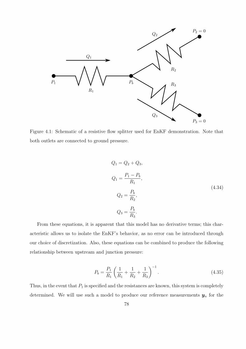
P1 Pb

R1

R2

R3

Q1

Q2

Q3

P2 = 0

P3 = 0

Figure 4.1: Schematic of a resistive flow splitter used for EnKF demonstration. Note that

both outlets are connected to ground pressure.

Q1 = Q2 +Q3,

Q1 =P1 − PbR1

,

Q2 =PbR2

,

Q3 =PbR3

.

(4.34)

From these equations, it is apparent that this model has no derivative terms; this char-

acteristic allows us to isolate the EnKF’s behavior, as no error can be introduced through

our choice of discretization. Also, these equations can be combined to produce the following

relationship between upstream and junction pressure:

Pb =P1

R1

(1

R1

+1

R2

+1

R3

)−1

. (4.35)

Thus, in the event that P1 is specified and the resistances are known, this system is completely

determined. We will use such a model to produce our reference measurements yn for the

78

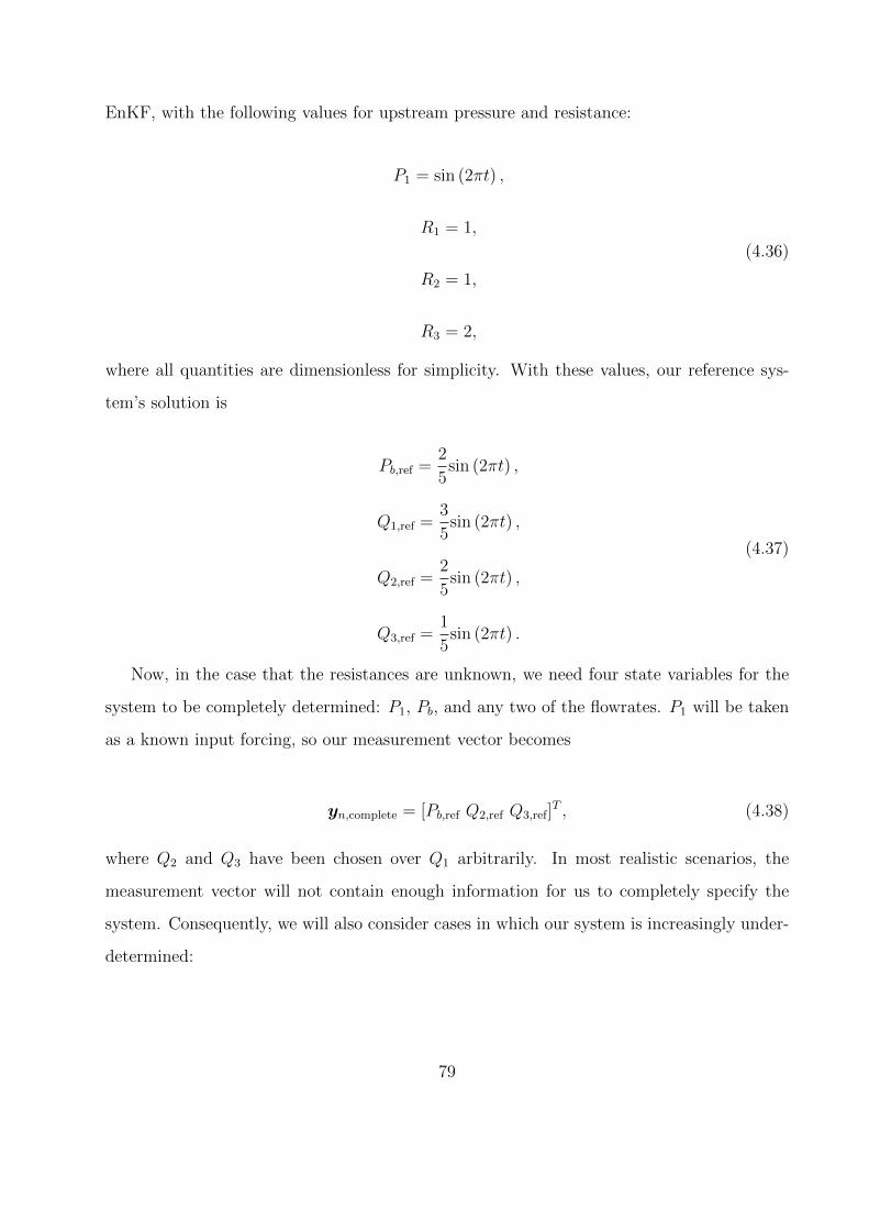
EnKF, with the following values for upstream pressure and resistance:

P1 = sin (2πt) ,

R1 = 1,

R2 = 1,

R3 = 2,

(4.36)

where all quantities are dimensionless for simplicity. With these values, our reference sys-

tem’s solution is

Pb,ref =2

5sin (2πt) ,

Q1,ref =3

5sin (2πt) ,

Q2,ref =2

5sin (2πt) ,

Q3,ref =1

5sin (2πt) .

(4.37)

Now, in the case that the resistances are unknown, we need four state variables for the

system to be completely determined: P1, Pb, and any two of the flowrates. P1 will be taken

as a known input forcing, so our measurement vector becomes

yn,complete = [Pb,ref Q2,ref Q3,ref]T , (4.38)

where Q2 and Q3 have been chosen over Q1 arbitrarily. In most realistic scenarios, the

measurement vector will not contain enough information for us to completely specify the

system. Consequently, we will also consider cases in which our system is increasingly under-

determined:

79

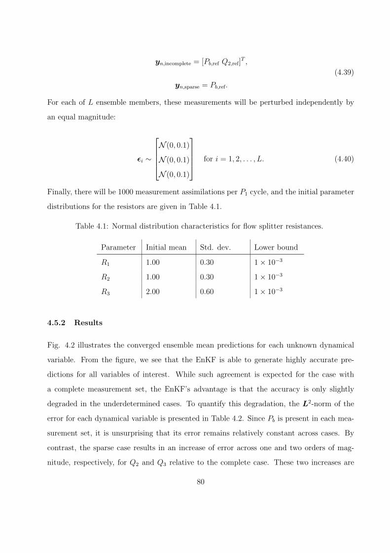
yn,incomplete = [Pb,ref Q2,ref]T ,

yn,sparse = Pb,ref.

(4.39)

For each of L ensemble members, these measurements will be perturbed independently by

an equal magnitude:

εi ∼

N (0, 0.1)

N (0, 0.1)

N (0, 0.1)

for i = 1, 2, . . . , L. (4.40)

Finally, there will be 1000 measurement assimilations per P1 cycle, and the initial parameter

distributions for the resistors are given in Table 4.1.

Table 4.1: Normal distribution characteristics for flow splitter resistances.

Parameter Initial mean Std. dev. Lower bound

R1 1.00 0.30 1× 10−3

R2 1.00 0.30 1× 10−3

R3 2.00 0.60 1× 10−3

4.5.2 Results

Fig. 4.2 illustrates the converged ensemble mean predictions for each unknown dynamical

variable. From the figure, we see that the EnKF is able to generate highly accurate pre-

dictions for all variables of interest. While such agreement is expected for the case with

a complete measurement set, the EnKF’s advantage is that the accuracy is only slightly

degraded in the underdetermined cases. To quantify this degradation, the L2-norm of the

error for each dynamical variable is presented in Table 4.2. Since Pb is present in each mea-

surement set, it is unsurprising that its error remains relatively constant across cases. By

contrast, the sparse case results in an increase of error across one and two orders of mag-

nitude, respectively, for Q2 and Q3 relative to the complete case. These two increases are

80

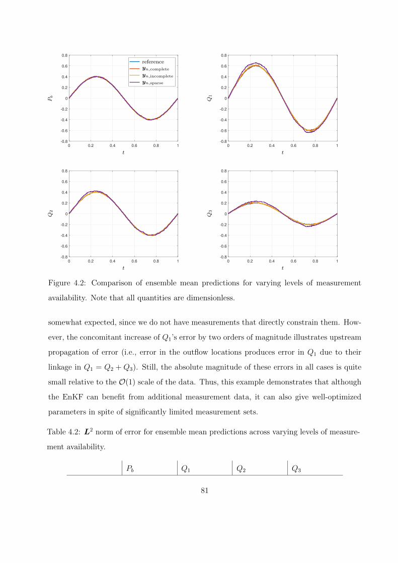
0 0.2 0.4 0.6 0.8 1

-0.8

-0.6

-0.4

-0.2

0

0.2

0.4

0.6

0.8

-------------------

Pb

t

referenceyn,complete

yn,incomplete

yn,sparse

0 0.2 0.4 0.6 0.8 1

-0.8

-0.6

-0.4

-0.2

0

0.2

0.4

0.6

0.8

Q1

t

0 0.2 0.4 0.6 0.8 1

-0.8

-0.6

-0.4

-0.2

0

0.2

0.4

0.6

0.8

Q2

t

0 0.2 0.4 0.6 0.8 1

-0.8

-0.6

-0.4

-0.2

0

0.2

0.4

0.6

0.8

Q3

t

Figure 4.2: Comparison of ensemble mean predictions for varying levels of measurement

availability. Note that all quantities are dimensionless.

somewhat expected, since we do not have measurements that directly constrain them. How-

ever, the concomitant increase of Q1’s error by two orders of magnitude illustrates upstream

propagation of error (i.e., error in the outflow locations produces error in Q1 due to their

linkage in Q1 = Q2 + Q3). Still, the absolute magnitude of these errors in all cases is quite

small relative to the O(1) scale of the data. Thus, this example demonstrates that although

the EnKF can benefit from additional measurement data, it can also give well-optimized

parameters in spite of significantly limited measurement sets.

Table 4.2: L2 norm of error for ensemble mean predictions across varying levels of measure-

ment availability.

Pb Q1 Q2 Q3

81

complete 1.45× 10−5 1.93× 10−5 1.02× 10−5 7.55× 10−6

incomplete 1.16× 10−5 7.39× 10−5 1.24× 10−5 5.51× 10−5

sparse 1.21× 10−5 1.10× 10−3 2.07× 10−4 4.80× 10−4

82

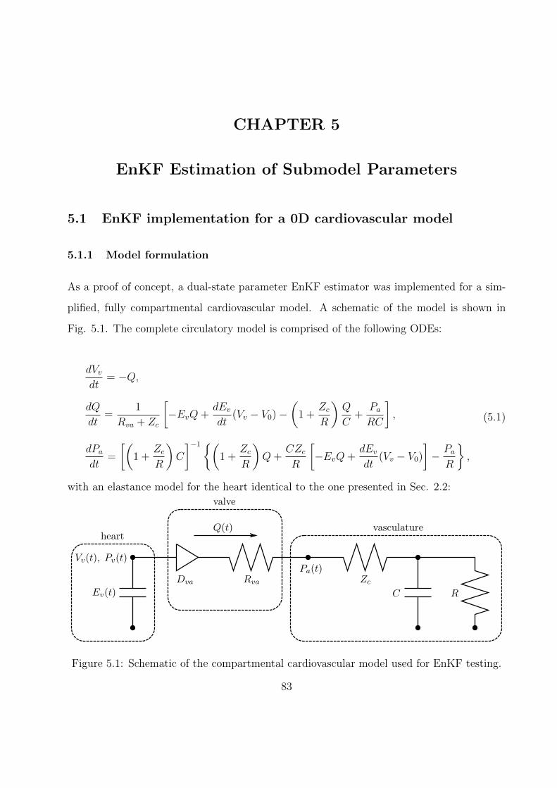
CHAPTER 5

EnKF Estimation of Submodel Parameters

5.1 EnKF implementation for a 0D cardiovascular model


As a proof of concept, a dual-state parameter EnKF estimator was implemented for a sim-

plified, fully compartmental cardiovascular model. A schematic of the model is shown in

Fig. 5.1. The complete circulatory model is comprised of the following ODEs:

dVvdt

= −Q,

dQ

dt=

1

Rva + Zc

[−EvQ+

dEvdt

(Vv − V0)−(

1 +ZcR

)Q

C+

PaRC

],

dPadt

=

[(1 +

ZcR

)C

]−1{(1 +

ZcR

)Q+

CZcR

[−EvQ+

dEvdt

(Vv − V0)

]− PaR

},

(5.1)

with an elastance model for the heart identical to the one presented in Sec. 2.2:

Ev(t)

Vv(t), Pv(t)

Q(t)

Dva Rva ZcC R

Pa(t)

heart

valve

vasculature

Figure 5.1: Schematic of the compartmental cardiovascular model used for EnKF testing.

83

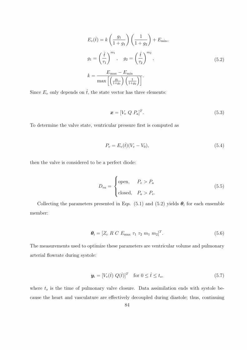
Ev(t) = k

(g1

1 + g1

)(1

1 + g2

)+ Emin,

g1 =

(t

τ1

)m1

, g2 =

(t

τ2

)m2

,

k =Emax − Emin

max[(

g11+g1

)(1

1+g2

)] .(5.2)

Since Ev only depends on t, the state vector has three elements:

x = [Vv Q Pa]T . (5.3)

To determine the valve state, ventricular pressure first is computed as

Pv = Ev(t)(Vv − V0), (5.4)

then the valve is considered to be a perfect diode:

Dva =

open, Pv > Pa

closed, Pa > Pv.

(5.5)

Collecting the parameters presented in Eqs. (5.1) and (5.2) yields θi for each ensemble

member:

θi = [Zc R C Emax τ1 τ2 m1 m2]T . (5.6)

The measurements used to optimize these parameters are ventricular volume and pulmonary

arterial flowrate during systole:

yi = [Vv(t) Q(t)]T for 0 ≤ t ≤ ts, (5.7)

where ts is the time of pulmonary valve closure. Data assimilation ends with systole be-

cause the heart and vasculature are effectively decoupled during diastole; thus, continuing

84

assimilation could introduce spurious correlations between ventricular measurements and

vascular parameters and vice-versa. The measurement vector was predicated upon clinical

availability of measurements: equivalent MRI data was taken from two volunteers, one nor-

motensive and one exhibiting pulmonary arterial hypertension. Based on knowledge of the

MRI measurement system, the perturbations εi added to the clinical measurement yn are

drawn from

εi ∼

N (0 cm3, 2.5 cm3)

N (0 cm3/s, 2.5 cm3/s)

for i = 1, 2, . . . , L. (5.8)

Each ensemble member is integrated forward in time using the 4th/5th-order adaptive

Runge-Kutta Cash Karp method, with clinical measurements sampled for assimilation at

approximately 80 Hz. Finally, since the model is an open-loop circulation (i.e., blood does

not return to the ventricle during diastole), each ensemble member is randomly re-initialzed

at the start of each cardiac cycle:

Vv,i(t = 0) ∼ N (135 mL, 10 mL) for i = 1, 2, . . . , L. (5.9)

The parameters for this submodel are tabulated with their descriptions, distribution prop-

erties, and converged values in Tables 5.2 through 5.4. Due to the availability of clinical

measurements, these parameters were chosen to be characteristic of the right ventricle and

pulmonary circulation. However, if measurement data were available for the systemic circu-

lation, the model could also be used there (with appropriately altered parameters).

5.1.2 Results

As a check on the stability of the estimation procedure, Fig. 5.2 shows the evolution of

the variance for a representative selection of model parameters in both the healthy and

hypertensive cases. The Hill function parameters m2 and τ2 have been omitted from this

subset, but their respective behaviors follow m1 and τ1. All variances have been normalized

by the initial ensemble mean for comparison, and indicate that the ensemble parameter

85

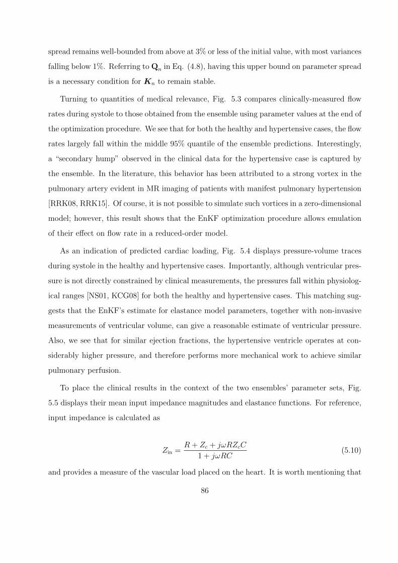
spread remains well-bounded from above at 3% or less of the initial value, with most variances

falling below 1%. Referring to Qn in Eq. (4.8), having this upper bound on parameter spread

is a necessary condition for Kn to remain stable.

Turning to quantities of medical relevance, Fig. 5.3 compares clinically-measured flow

rates during systole to those obtained from the ensemble using parameter values at the end of

the optimization procedure. We see that for both the healthy and hypertensive cases, the flow

rates largely fall within the middle 95% quantile of the ensemble predictions. Interestingly,

a “secondary hump” observed in the clinical data for the hypertensive case is captured by

the ensemble. In the literature, this behavior has been attributed to a strong vortex in the

pulmonary artery evident in MR imaging of patients with manifest pulmonary hypertension

[RRK08, RRK15]. Of course, it is not possible to simulate such vortices in a zero-dimensional

model; however, this result shows that the EnKF optimization procedure allows emulation

of their effect on flow rate in a reduced-order model.

As an indication of predicted cardiac loading, Fig. 5.4 displays pressure-volume traces

during systole in the healthy and hypertensive cases. Importantly, although ventricular pres-

sure is not directly constrained by clinical measurements, the pressures fall within physiolog-

ical ranges [NS01, KCG08] for both the healthy and hypertensive cases. This matching sug-

gests that the EnKF’s estimate for elastance model parameters, together with non-invasive

measurements of ventricular volume, can give a reasonable estimate of ventricular pressure.

Also, we see that for similar ejection fractions, the hypertensive ventricle operates at con-

siderably higher pressure, and therefore performs more mechanical work to achieve similar

pulmonary perfusion.

To place the clinical results in the context of the two ensembles’ parameter sets, Fig.

5.5 displays their mean input impedance magnitudes and elastance functions. For reference,

input impedance is calculated as

Zin =R + Zc + jωRZcC

1 + jωRC(5.10)

and provides a measure of the vascular load placed on the heart. It is worth mentioning that

86

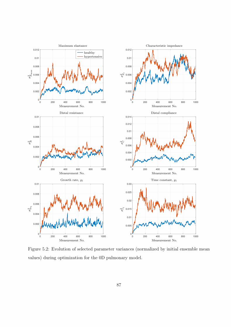
0 200 400 600 800 1000

0

0.002

0.004

0.006

0.008

0.01

0.012

hypertensive

------------

σ2 E

max

Measurement No.

Maximum elastance

healthy

hypertensive

0 200 400 600 800 1000

0

0.002

0.004

0.006

0.008

0.01

0.012

σ2 Zc

Measurement No.

Characteristic impedance

0 200 400 600 800 1000

0

0.002

0.004

0.006

0.008

0.01

σ2 R

Measurement No.

Distal resistance

0 200 400 600 800 1000

0

0.002

0.004

0.006

0.008

0.01

0.012

0.014

σ2 C

Measurement No.

Distal compliance

0 200 400 600 800 1000

0

0.002

0.004

0.006

0.008

0.01

σ2 m

1

Measurement No.

Growth rate, g1

0 200 400 600 800 1000

0

0.005

0.01

0.015

0.02

0.025

0.03

σ2 τ1

Measurement No.

Time constant, g1

Figure 5.2: Evolution of selected parameter variances (normalized by initial ensemble mean

values) during optimization for the 0D pulmonary model.

87

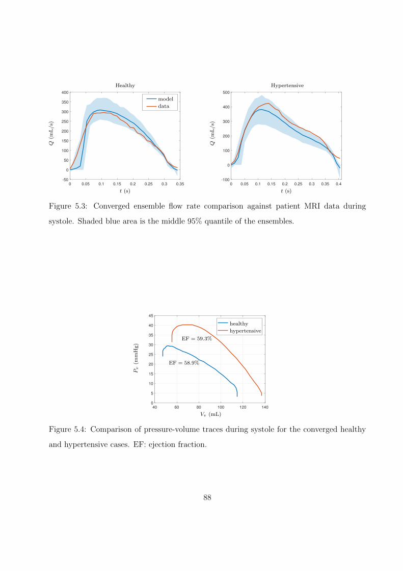
0 0.05 0.1 0.15 0.2 0.25 0.3 0.35

-50

0

50

100

150

200

250

300

350

400

--------

Q(m

L/s)

t (s)

Healthy

model

data

0 0.05 0.1 0.15 0.2 0.25 0.3 0.35 0.4

-100

0

100

200

300

400

500

Q(m

L/s)

t (s)

Hypertensive

Figure 5.3: Converged ensemble flow rate comparison against patient MRI data during

systole. Shaded blue area is the middle 95% quantile of the ensembles.

40 60 80 100 120 140

0

5

10

15

20

25

30

35

40

45

----------------

Pv

(mm

Hg)

Vv (mL)

healthy

hypertensive

EF = 58.9%

EF = 59.3%

Figure 5.4: Comparison of pressure-volume traces during systole for the converged healthy

and hypertensive cases. EF: ejection fraction.

88

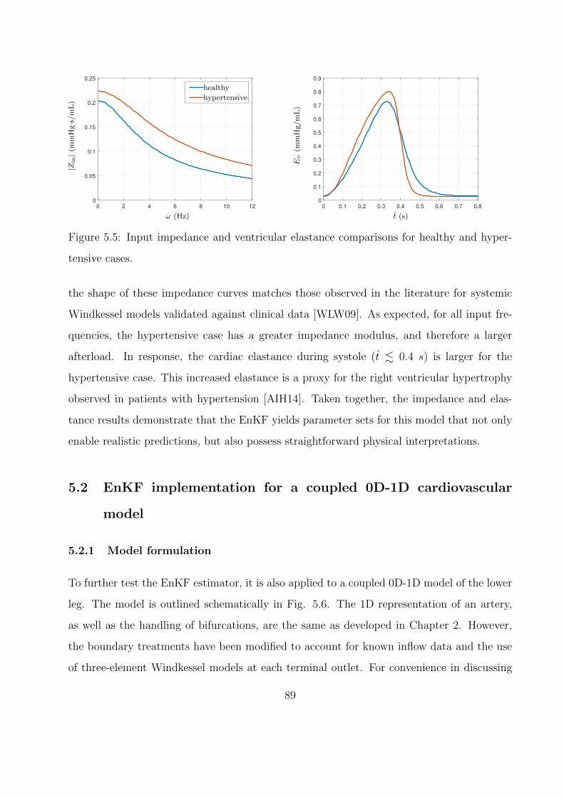
0 2 4 6 8 10 12

0

0.05

0.1

0.15

0.2

0.25

--------------

|Zin|(

mm

Hg·s

/m

L)

ω (Hz)

healthy

hypertensive

0 0.1 0.2 0.3 0.4 0.5 0.6 0.7 0.8

0

0.1

0.2

0.3

0.4

0.5

0.6

0.7

0.8

0.9

Ev

(mm

Hg/m

L)

t (s)

Figure 5.5: Input impedance and ventricular elastance comparisons for healthy and hyper-

tensive cases.

the shape of these impedance curves matches those observed in the literature for systemic

Windkessel models validated against clinical data [WLW09]. As expected, for all input fre-

quencies, the hypertensive case has a greater impedance modulus, and therefore a larger

afterload. In response, the cardiac elastance during systole (t . 0.4 s) is larger for the

hypertensive case. This increased elastance is a proxy for the right ventricular hypertrophy

observed in patients with hypertension [AIH14]. Taken together, the impedance and elas-

tance results demonstrate that the EnKF yields parameter sets for this model that not only

enable realistic predictions, but also possess straightforward physical interpretations.

5.2 EnKF implementation for a coupled 0D-1D cardiovascular

model


To further test the EnKF estimator, it is also applied to a coupled 0D-1D model of the lower

leg. The model is outlined schematically in Fig. 5.6. The 1D representation of an artery,

as well as the handling of bifurcations, are the same as developed in Chapter 2. However,

the boundary treatments have been modified to account for known inflow data and the use

of three-element Windkessel models at each terminal outlet. For convenience in discussing

89

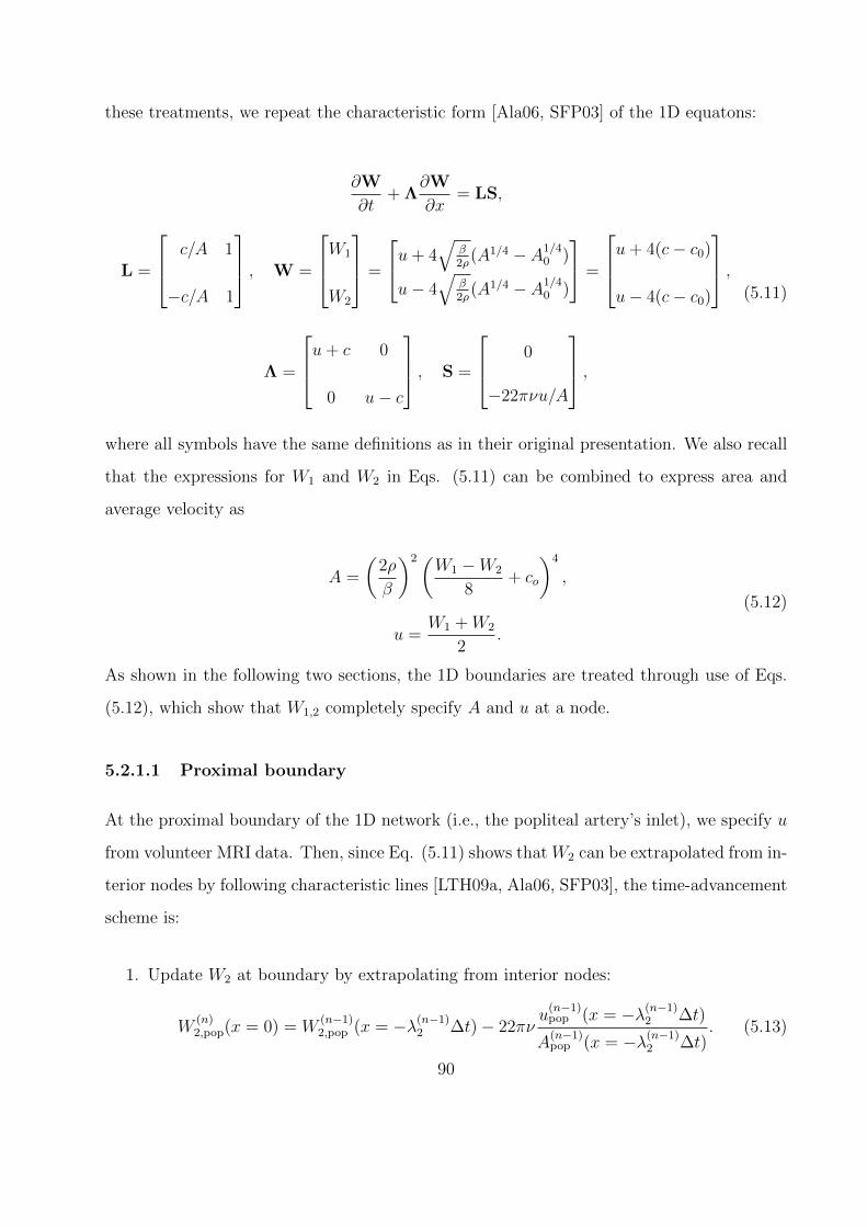
these treatments, we repeat the characteristic form [Ala06, SFP03] of the 1D equatons:

∂W

∂t+ Λ

∂W

∂x= LS,

L =

c/A 1

−c/A 1

, W =

W1

W2

=

u+ 4√

β2ρ

(A1/4 − A1/40 )

u− 4√

β2ρ

(A1/4 − A1/40 )

=

u+ 4(c− c0)

u− 4(c− c0)

,

Λ =

u+ c 0

0 u− c

, S =

0

−22πνu/A

,(5.11)

where all symbols have the same definitions as in their original presentation. We also recall

that the expressions for W1 and W2 in Eqs. (5.11) can be combined to express area and

average velocity as

A =

(2ρ

β

)2(W1 −W2

8+ co

)4

,

u =W1 +W2

2.

(5.12)

As shown in the following two sections, the 1D boundaries are treated through use of Eqs.

(5.12), which show that W1,2 completely specify A and u at a node.

5.2.1.1 Proximal boundary

At the proximal boundary of the 1D network (i.e., the popliteal artery’s inlet), we specify u

from volunteer MRI data. Then, since Eq. (5.11) shows that W2 can be extrapolated from in-

terior nodes by following characteristic lines [LTH09a, Ala06, SFP03], the time-advancement

scheme is:

1. Update W2 at boundary by extrapolating from interior nodes:

W(n)2,pop(x = 0) = W

(n−1)2,pop (x = −λ(n−1)

2 ∆t)− 22πνu

(n−1)pop (x = −λ(n−1)

2 ∆t)

A(n−1)pop (x = −λ(n−1)

2 ∆t). (5.13)

90

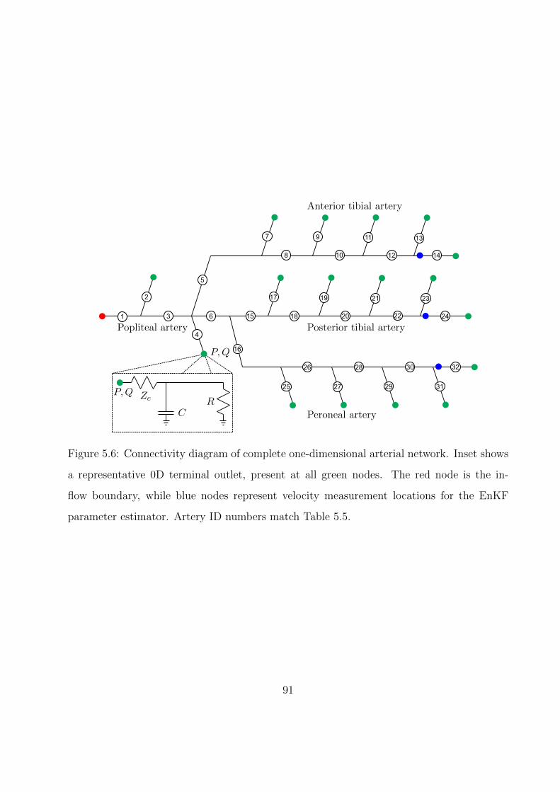
8

1

2

3

4

5

6

7 9

10

11

12

13

14

15

16

17

18

19

20

21

22

23

24

25 27 29 31

26 28 30 32

Popliteal artery

Anterior tibial artery

Posterior tibial artery

Peroneal artery

P,Q

P,Q Zc

CR

Figure 5.6: Connectivity diagram of complete one-dimensional arterial network. Inset shows

a representative 0D terminal outlet, present at all green nodes. The red node is the in-

flow boundary, while blue nodes represent velocity measurement locations for the EnKF

parameter estimator. Artery ID numbers match Table 5.5.

91

2. Set W1 and update A at the proximal boundary according to Eqs. (5.12):

W(n)1,pop(x = 0) = 2u(n)

pop −W(n)2,pop(x = 0),

A(n)pop(x = 0) =

(2ρ

βpop

)2(W

(n)1,pop(x = 0)−W (n)

2,pop(x = 0)

8+ c0,pop

)4

.

(5.14)

5.2.1.2 Distal boundary

At the distal end of the 1D network, we couple terminal arteries to three-element Windkessel

models, as sketched in Fig. 5.6. To do so, we begin with an implicit Euler discretization for

the governing ODE of a three-element Windkessel (all notation follows Fig. 5.6):

P (n) + ZcCP (n) − P (n−1)

∆t= (Zc +R)Q(n) + ZcRC

Q(n) −Q(n−1)

∆t. (5.15)

Coupling between the 0D and 1D domains occurs through the following substitutions into Eq.

(5.15), based on the characteristic relations in Eqs. (5.12) alongside the arterial pressure-area

relationship presented in Chapter 2:

P (n) = β(√A(n) −

√A0),

A(n) =

(2ρ

β

)2(W

(n)1 −W (n)

2

8+ co

)4

,

Q(n) = A(n)u(n) = A(n)W(n)1 +W

(n)2

2.

(5.16)

Since W(n)1 can be extrapolated from interior nodes, Eqs. (5.15) and (5.16) form a single

nonlinear equation for W(n)2 :

92

2ρ

(1 +

RC

∆t

)(W

(n)1 −W (n)

2

8+ co

)2

−

(2ρ

β

)2(Zc +R +

ZcRC

∆t

)(W

(n)1 −W (n)

2

8+ co

)4(W

(n)1 +W

(n)2

2

)+ P (n−1) = 0,

P (n−1) =ZcRC

∆tQ(n−1) − RC

∆tP (n−1) −

(1 +

RC

∆t

)β√A0.

(5.17)

The above equation is solved with Newton-Raphson iteration, using values at the previous

time step as an initial guess.

5.2.1.3 0D-1D parameter estimation

Compared to the 0D pulmonary model, the coupled 0D-1D leg model has a considerably

larger parameter space for optimization. Specifically, there are 17 total terminal Windkessel

models whose R and C require estimation (Zc is fixed to the artery’s characteristic impedance

ρc0/A0 to avoid spurious reflections [APP08]), plus 32 1D segments whose stiffness parameter

β needs estimation. However, the measurement set is of comparable size to the pure 0D test,

consisting of simultaneous planar MRI blood velocity measurements along the anterior tibial,

posterior tibial, and peroneal arteries:

y = [uant upost uper]T . (5.18)

For the data perturbations εi, the distributions were given a standard deviation of 2.5 cm/s:

εi ∼

N (0 cm3, 2.5 cm3/s)

N (0 cm3, 2.5 cm3/s)

N (0 cm3, 2.5 cm3/s)

for i = 1, 2, . . . , L. (5.19)

The clinical measurements above are mapped onto the 1D arterial network at the inlet nodes

to segments 14, 24, and 32 (the blue nodes in Fig. 5.6), i.e.

93

yi = [u14,i(x = 0) u24,i(x = 0) u32,i(x = 0)]T for i = 1, 2, . . . , L. (5.20)

To make the optimization procedure tractable, initial values are first manually assigned

for R, C, and β so that 1) mean arterial pressure falls in a realistic range between 90

and 95 mmHg, and 2) the minimum arterial wave speed c0 is well-matched near 8 m/s

[KKJ07]. To proceed, we recall that the LH-OAT sensitivity analysis in Sec. 3.4 indicated

that Windkessel compliance and arterial stiffness strongly influence arterial measurements of

pressure and peak flow (A0 is excluded to simplify the tuning procedure, as its impact could

not be distinguished from that of β). We also note that the time-mean of a three-element

Windkessel yields

Q =P

Zc +R. (5.21)

However, since Zc is fixed to avoid spurious reflections, the mean component of flow in

this case can only be adjusted through changes to R. Therefore, in each of the segments

onto which the velocity measurements are mapped, we will directly tune C, R, and β, such

that a portion of the parameter vector is

θa = [R14 C14 R24 C24 R32 C32 β14 β24 β32]T . (5.22)

Note the ensemble index i has been dropped for brevity. For the remaining terminals, a

scaling parameter is introduced for all R and C values within a given artery:

θb = [αR,ant αC,ant, αR,post αC,post, αR,per αC,per]T . (5.23)

These parameters are used to uniformly scale all terminals upstream of a measurement site.

For example, the anterior tibial scalings are applied as

Rj ← αR,antRj

Cj ← αC,antCj

for j = 7, 9, 11, 13. (5.24)

94

The posterior tibial, peroneal, and popliteal arteries follow the same procedure, with the

popliteal scalings given by the average value in the remaining three arteries. The complete

parameter vector thus contains only 15 parameters, given by the concatenation of θa and θb:

θ = [θa θb]T . (5.25)

Finally, to ensure the arterial wave speed remains well-matched, β for upstream segments

is scaled by the fractional change in the corresponding measured segment. Again using the

anterior tibial artery for illustration:

βj ←β+

14 − β−14

β−14

βj for j = 7, 9, 11, 13. (5.26)

The posterior tibial and peroneal stiffness parameters are changed similarly, and the popliteal

segments are then altered according to the average fractional change across the three down-

stream arteries.

5.2.2 Results

To demonstrate the converged ensemble’s predictive utility, Fig. 5.7 compares model veloci-

ties at the measurement locations against patient MRI data. For all measurement locations,

it can be seen that the model does reasonably well at capturing waveform shape and peak

velocities. Though some overshoot exists in terms of systolic pulse duration and maximum

backflow rate, Table 5.1 shows that the time-averaged velocity (and hence mean perfusion)

is well-matched, especially for the anterior tibial and peroneal arteries. It is also worth

emphasizing that these results were produced with an extremely limited measurement set:

the measurement vector dimension is O(1), while the overall parameter space dimension is

O(100). Thus, these predictions could likely be improved through additional measurements

with which to constrain the parameter estimation procedure.

As in the fully 0D problem, the ensemble generated for this case is able to output es-

timates of patient pressure. The pressure waveforms are given in Fig. 5.8, and fall within

95

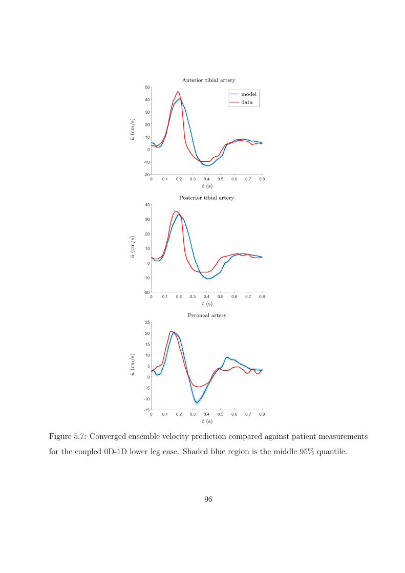
0 0.1 0.2 0.3 0.4 0.5 0.6 0.7 0.8

-20

-10

0

10

20

30

40

50

---------

u(c

m/s)

t (s)

Anterior tibial artery

model

data

0 0.1 0.2 0.3 0.4 0.5 0.6 0.7 0.8

-20

-10

0

10

20

30

40

u(c

m/s)

t (s)

Posterior tibial artery

0 0.1 0.2 0.3 0.4 0.5 0.6 0.7 0.8

-15

-10

-5

0

5

10

15

20

25

u(c

m/s)

t (s)

Peroneal artery

Figure 5.7: Converged ensemble velocity prediction compared against patient measurements

for the coupled 0D-1D lower leg case. Shaded blue region is the middle 95% quantile.

96

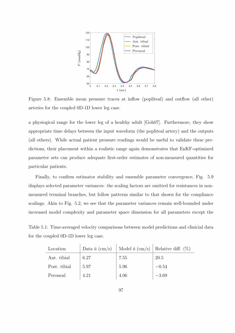
0 0.1 0.2 0.3 0.4 0.5 0.6 0.7 0.8

50

60

70

80

90

100

110

120

------------------

P(m

mH

g)

t (sec)

Popliteal

Ant. tibial

Post. tibial

Peroneal

Figure 5.8: Ensemble mean pressure traces at inflow (popliteal) and outflow (all other)

arteries for the coupled 0D-1D lower leg case.

a physiogical range for the lower leg of a healthy adult [Goh07]. Furthermore, they show

appropriate time delays between the input waveform (the popliteal artery) and the outputs

(all others). While actual patient pressure readings would be useful to validate these pre-

dictions, their placement within a realistic range again demonstrates that EnKF-optimized

parameter sets can produce adequate first-order estimates of non-measured quantities for

particular patients.

Finally, to confirm estimator stability and ensemble parameter convergence, Fig. 5.9

displays selected parameter variances: the scaling factors are omitted for resistances in non-

measured terminal branches, but follow patterns similar to that shown for the compliance

scalings. Akin to Fig. 5.2, we see that the parameter variances remain well-bounded under

increased model complexity and parameter space dimension for all parameters except the

Table 5.1: Time-averaged velocity comparisons between model predictions and clinicial data

for the coupled 0D-1D lower leg case.

Location Data u (cm/s) Model u (cm/s) Relative diff. (%)

Ant. tibial 6.27 7.55 20.5

Post. tibial 5.97 5.96 −0.54

Peroneal 4.21 4.06 −3.69

97

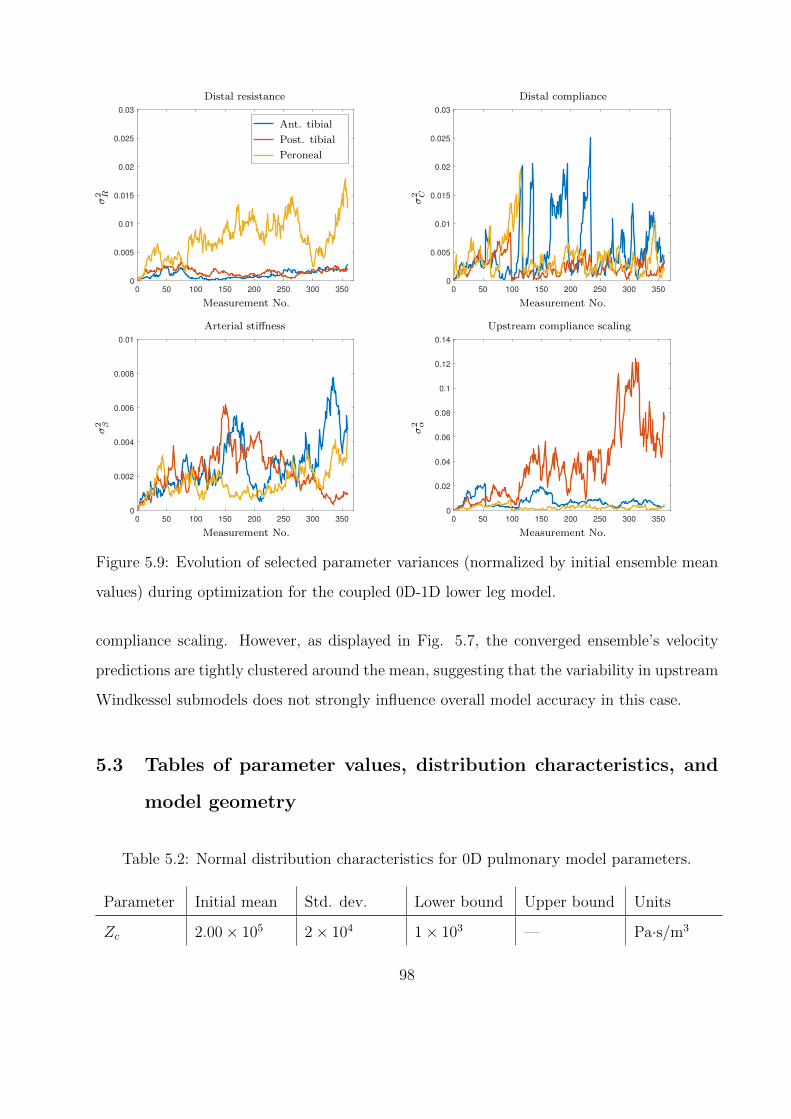
0 50 100 150 200 250 300 350

0

0.005

0.01

0.015

0.02

0.025

0.03

------------------

σ2 R

Measurement No.

Distal resistance

Ant. tibial

Post. tibial

Peroneal

0 50 100 150 200 250 300 350

0

0.005

0.01

0.015

0.02

0.025

0.03

σ2 C

Measurement No.

Distal compliance

0 50 100 150 200 250 300 350

0

0.002

0.004

0.006

0.008

0.01

σ2 β

Measurement No.

Arterial stiffness

0 50 100 150 200 250 300 350

0

0.02

0.04

0.06

0.08

0.1

0.12

0.14

σ2 α

Measurement No.

Upstream compliance scaling

Figure 5.9: Evolution of selected parameter variances (normalized by initial ensemble mean

values) during optimization for the coupled 0D-1D lower leg model.

compliance scaling. However, as displayed in Fig. 5.7, the converged ensemble’s velocity

predictions are tightly clustered around the mean, suggesting that the variability in upstream

Windkessel submodels does not strongly influence overall model accuracy in this case.

5.3 Tables of parameter values, distribution characteristics, and

model geometry

Table 5.2: Normal distribution characteristics for 0D pulmonary model parameters.

Parameter Initial mean Std. dev. Lower bound Upper bound Units

Zc 2.00× 105 2× 104 1× 103 — Pa·s/m3

98

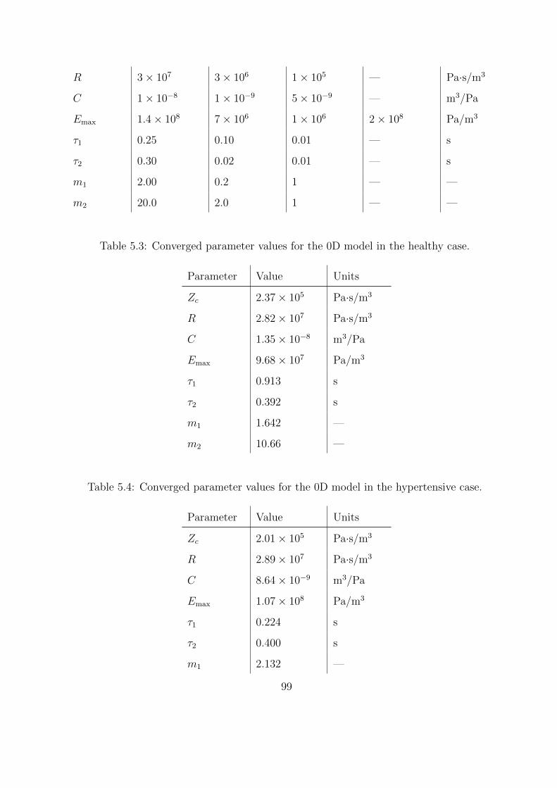
R 3× 107 3× 106 1× 105 — Pa·s/m3

C 1× 10−8 1× 10−9 5× 10−9 — m3/Pa

Emax 1.4× 108 7× 106 1× 106 2× 108 Pa/m3

τ1 0.25 0.10 0.01 — s

τ2 0.30 0.02 0.01 — s

m1 2.00 0.2 1 — —

m2 20.0 2.0 1 — —

Table 5.3: Converged parameter values for the 0D model in the healthy case.


Zc 2.37× 105 Pa·s/m3

R 2.82× 107 Pa·s/m3

C 1.35× 10−8 m3/Pa

Emax 9.68× 107 Pa/m3

τ1 0.913 s

τ2 0.392 s

m1 1.642 —

m2 10.66 —

Table 5.4: Converged parameter values for the 0D model in the hypertensive case.


Zc 2.01× 105 Pa·s/m3

R 2.89× 107 Pa·s/m3

C 8.64× 10−9 m3/Pa

Emax 1.07× 108 Pa/m3

τ1 0.224 s

τ2 0.400 s

m1 2.132 —

99

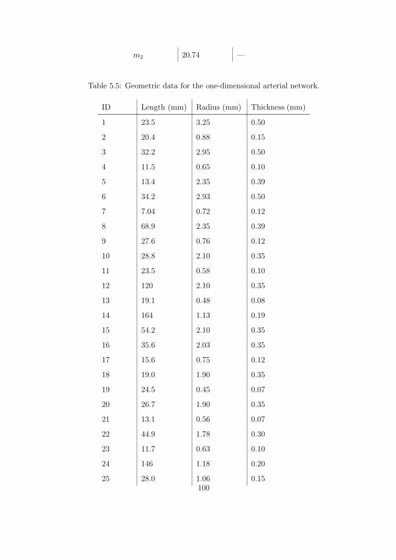
m2 20.74 —

Table 5.5: Geometric data for the one-dimensional arterial network.

ID Length (mm) Radius (mm) Thickness (mm)

1 23.5 3.25 0.50

2 20.4 0.88 0.15

3 32.2 2.95 0.50

4 11.5 0.65 0.10

5 13.4 2.35 0.39

6 34.2 2.93 0.50

7 7.04 0.72 0.12

8 68.9 2.35 0.39

9 27.6 0.76 0.12

10 28.8 2.10 0.35

11 23.5 0.58 0.10

12 120 2.10 0.35

13 19.1 0.48 0.08

14 164 1.13 0.19

15 54.2 2.10 0.35

16 35.6 2.03 0.35

17 15.6 0.75 0.12

18 19.0 1.90 0.35

19 24.5 0.45 0.07

20 26.7 1.90 0.35

21 13.1 0.56 0.07

22 44.9 1.78 0.30

23 11.7 0.63 0.10

24 146 1.18 0.20

25 28.0 1.06 0.15100

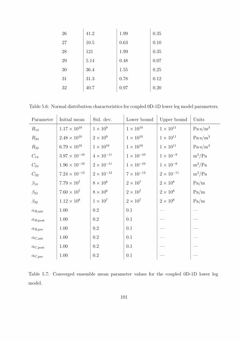
26 41.2 1.99 0.35

27 10.5 0.63 0.10

28 121 1.99 0.35

29 5.14 0.48 0.07

30 36.4 1.55 0.25

31 31.3 0.78 0.12

32 40.7 0.97 0.20

Table 5.6: Normal distribution characteristics for coupled 0D-1D lower leg model parameters.

Parameter Initial mean Std. dev. Lower bound Upper bound Units

R14 1.17× 1010 1× 109 1× 1010 1× 1011 Pa·s/m3

R24 2.48× 1010 2× 109 1× 1010 1× 1011 Pa·s/m3

R32 6.79× 1010 1× 1010 1× 1010 1× 1011 Pa·s/m3

C14 3.97× 10−10 4× 10−11 1× 10−10 1× 10−9 m3/Pa

C24 1.96× 10−10 2× 10−11 1× 10−10 1× 10−9 m3/Pa

C32 7.24× 10−12 2× 10−12 7× 10−12 2× 10−11 m3/Pa

β14 7.79× 107 8× 106 2× 107 2× 108 Pa/m

β24 7.60× 107 8× 106 2× 107 2× 108 Pa/m

β32 1.12× 108 1× 107 2× 107 2× 108 Pa/m

αR,ant 1.00 0.2 0.1 — —

αR,post 1.00 0.2 0.1 — —

αR,per 1.00 0.2 0.1 — —

αC,ant 1.00 0.2 0.1 — —

αC,post 1.00 0.2 0.1 — —

αC,per 1.00 0.2 0.1 — —

Table 5.7: Converged ensemble mean parameter values for the coupled 0D-1D lower leg

model.

101

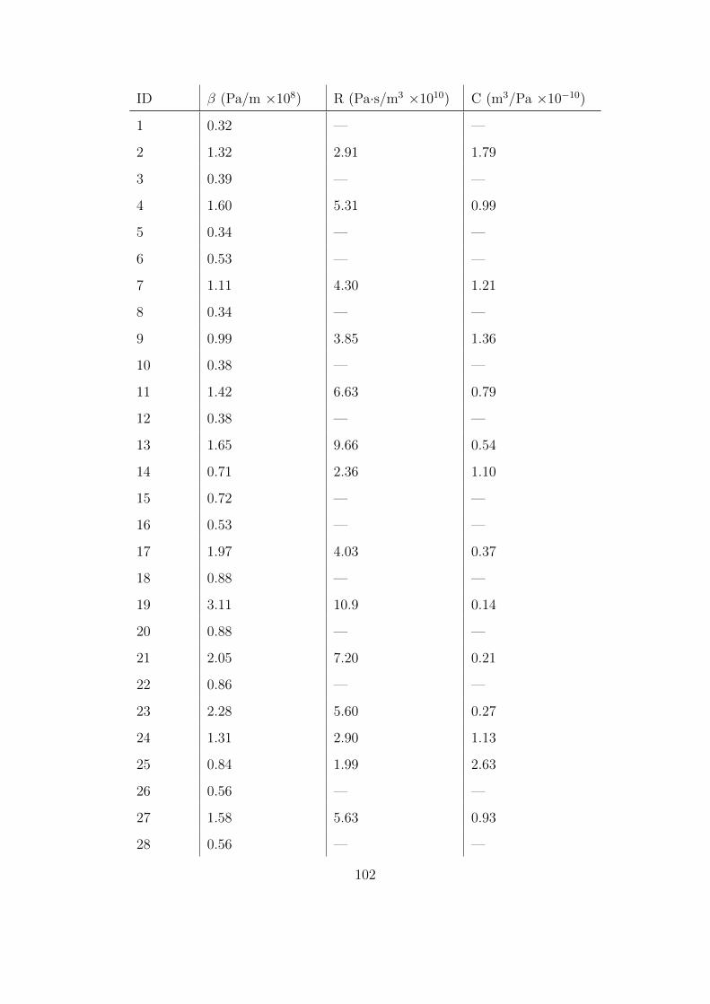
ID β (Pa/m ×108) R (Pa·s/m3 ×1010) C (m3/Pa ×10−10)

1 0.32 — —

2 1.32 2.91 1.79

3 0.39 — —

4 1.60 5.31 0.99

5 0.34 — —

6 0.53 — —

7 1.11 4.30 1.21

8 0.34 — —

9 0.99 3.85 1.36

10 0.38 — —

11 1.42 6.63 0.79

12 0.38 — —

13 1.65 9.66 0.54

14 0.71 2.36 1.10

15 0.72 — —

16 0.53 — —

17 1.97 4.03 0.37

18 0.88 — —

19 3.11 10.9 0.14

20 0.88 — —

21 2.05 7.20 0.21

22 0.86 — —

23 2.28 5.60 0.27

24 1.31 2.90 1.13

25 0.84 1.99 2.63

26 0.56 — —

27 1.58 5.63 0.93

28 0.56 — —

102

29 1.92 9.75 0.54

30 0.66 — —

31 1.24 5.35 0.97

32 1.35 7.17 7.73× 10−2

103

CHAPTER 6

Conclusion

6.1 Summary and Future Work

With reference to the research objectives outlined in Sec. 1.3, the work presented here has

demonstrated significant progress. Specifically, we have achieved the following goals:

• Coupled a one-dimensional submodel of the major arteries to zero-dimensional submod-

els of the peripheral vasculature, heart, and lungs to create a closed-loop cardiovascular

model capable of providing organ-level fluid dynamical data

• Employed a reduced-order baroreflex model to predict cardiovascular behavior due to

neurogenic hypertension and acute hemorrhage

• Implemented the ensemble Kalman filter (EnKF) to enable data-driven parameter

tuning for patient-specific models of the pulmonary vasculature and lower leg

Furthermore, validation of the closed-loop model against literature data showed that it is

capable of reasonably reproducing both global and local (at the spatial resolution of the major

arteries) cardiovascular dynamics measured in vivo. Demonstration of the latter capability

is especially important, as it indicates that this model is suitable for embedding within a

three-dimensional organ model (i.e., it will be able to predict the perfusion of the organ’s

tissue, and react appropriately if the tissue is damaged). No available literature to date has

achieved this type of coupling, making it an important direction for future effort.

In addition to coupling with a higher-order organ model, the current cardiovascular model

could be improved or extended by:

104

• Implementation of a model for cerebral autoregulation to enable the cerebral vascu-

lature to act independently of the baroreflex, as expected from in vivo measurements

[MKF79]

• Usage of machine learning methods (e.g., evolutionary algorithms or artificial neural

networks) as computationally-efficient function approximators [DBN16] to replace the

nonlinear physical models used in the one-dimensional arterial network

The achievement of these additional objectives would allow the model to be more physically

accurate and less costly to compute. These improvements would allow rapid application

to a broad variety of clinical contexts, making it possible to assist medical practicioners in

performing diagnoses and planning treatments.

6.2 Publications and Presentations

The publications and presentations associated with this work are listed below.

1. Canuto, D., Chong, K., Bowles, C., Dutson, E. P., Eldredge, J. D., and Benharash, P.,

“A regulated multiscale closed-loop cardiovascular model, with applications to hemor-

rhage and hypertension, International Journal of Biomedical Engineering, 2018

2. Canuto, D., Pantoja, J. L., Han, J., Dutson, E. P., and Eldredge, J. D., An ensemble

Kalman filter approach to parameter optimization for patient-specific cardiovascular

modeling, 2019, in prep.

3. Canuto, D., Chang, Y., Eldredge, J., Dutson, E. P., and Benharash, P., A Parameter

Ensemble Kalman Filter for Patient-Specific Cardiovascular Modeling, 71st Annual

Meeting of the APS Division of Fluid Dynamics, Atlanta, GA, November 25-27, 2018.

Presentation.

4. Canuto, D., Chong, K., Bowles, C., Dutson, E. P., Eldredge, J. D., and Benharash, P.,

A Multiscale Closed-Loop Cardiovascular Model, with Applications to Hemorrhage and

105

Hypertension, 70th Annual Meeting of the APS Division of Fluid Dynamics, Denver,

CO, November 19-21, 2017. Presentation.

106

REFERENCES

[AA99] J. L. Anderson and S. L. Anderson. “A Monte Carlo implementation of the non-linear filtering problem to produce ensemble assimilations and forecasts.” Mon.Wea. Rev., 127:2741–2758, 1999.

[AHM76] F. M. Abboud, D. D. Heistad, A. L. Mark, and P. G. Schmid. “Reflex control ofthe peripheral circulation.” Prog. Cardio. Diseases, 18(5):371–403, 1976.

[AIH14] J. Aguero, K. Ishikawa, L. Hadri, C. Santos-Gallego, K. Fish, N. Hammoudi,A. Chaanine, S. Torquato, C. Naim, B. Ibanez, D. Pereda, A. Garcia-Alvarez,V. Fuster, P. P. Sengupta, J. A. Leopold, and R. J. Hajjar. “Characterizationof right ventricular remodeling and failure in a chronic pulmonary hypertensionmodel.” Am. J. Physiol. Heart Circ. Physiol., 307(8):H1204–H1215, 2014.

[Ala06] J. Alastruey. Numerical modelling of pulse wave propagation in the cardiovascularsystem: development, validation, and clinical applications. PhD thesis, ImperialCollege London, 2006.

[APP08] J. Alastruey, K. H. Parker, J. Peiro, and S. J. Sherwin. “Lumped parameter out-flow models for 1-D blood flow simulations: effect on pulse waves and parameterestimation.” Commun. Comp. Phys., 4(2):317–336, 2008.

[AT84] F. M. Abboud and M. D. Thames. Handbook of Physiology: Peripheral Circulationand Organ Blood Flow, volume 3, chapter 19, pp. 675–753. Americal PhysiologicalSociety, 1984.

[Avo80] A. P. Avolio. “Multi-branched model of the human arterial system.” Med. Biol.Eng. Comp., 18:709–718, 1980.

[BAP01] P. Boscan, A. M. Allen, and J. F. R. Paton. “Baroreflex inhibition of cardiacsympathetic outflow is attenuated by angiotensin II in the nucleus of the solitarytract.” Neuroscience, 103(1):153–160, 2001.

[BGC84] S. M. Barman, G. L. Gebber, and F. R. Calaresu. “Differential control of sympa-thetic nerve discharge by the brain stem.” Am. J. Physiol., 247, 1984.

[BHP69] J. D. Bristow, A. J. Honour, G. W. Pickering, P. Sleight, and H. S. Smyth.“Diminished baroreflex sensitivity in high blood pressure.” Circulation, 39:48–54, 1969.

[BKS07] J. J. Batzel, F. Kappel, D. Schneditz, and H. T. Tran. Cardiovascular and Res-piratory Systems: Modeling, Analysis, and Control. SIAM, 2007.

[BLE98] G. Burgers, P. Jan van Leeuwen, and G. Evensen. “Analysis scheme in the en-semble Kalman filter.” Mon. Wea. Rev., 126:1719–1724, 1998.

107

[BR80] R. L. Bras and P. Restrepo-Posada. “Real time automatic parameter calibrationin conceptual runoff forecasting models.” In Proceedings of the Third InternationalSymposium on Stochastic Hydraulics, pp. 61–70, 1980.

[BTD05] M. Banaji, A. Tachtsidis, D. Delpy, and S. Baigent. “A physiological model ofcerebral blood flow control.” Mathematical Biosciences, 194:125–173, 2005.

[BTF12] P. J. Blanco, P. R. Trenhago, L. G. Fernandes, and R. A. Feijoo. “On the in-tegration of the baroreflex control mechanism in a heterogeneous model of thecardiovascular system.” Int. J. Num. Meth. Biomed. Eng., 28:412–433, 2012.

[CAA00] H. L. Collins, R. A. Augustyniak, E. J. Ansorge, and D. S. O’Leary. “Carotidbaroreflex pressor responses at rest and during exercise: cardiac output vs. re-gional vasoconstriction.” Am. J. Physiol., 280, 2000.

[CAH09] P. A. Cain, R. Ahl, E. Hedstrom, M. Ugander, A. Allansdotter-Johnsson,P. Friberg, and H. Arheden. “Age and gender specific normal values of left ven-tricular mass, volume and function for gradient echo magnetic resonance imaging:a cross sectional study.” BMC Med. Imag., 9(2), 2009.

[CBB03] A. V. Chobanian, G. L. Bakris, H. R. Black, W. C. Cushman, L. A. Green, J. L.Izzo Jr., D. W. Jones, B. J. Materson, S. Oparil, J. T. Wright Jr., E. J. Roccella,and the National High Blood Pressure Education Program Coordinating Com-mittee. “Seventh report of the joint national committee on prevention, detection,evaluation, and treatment of high blood pressure.” Hypertension, 42:1206–1252,2003.

[CST87] J. Christie, L. M. Sheldahl, F. E. Tristani, K. B. Sagar, M. J. Ptacin, and S. Wann.“Determination of stroke volume and cardiac output during exercise: comparisonof two-dimensional and Doppler echocardiography, Fick oximetry, and thermodi-lution.” Circulation, 76(3):539–547, 1987.

[Dam94] R. A. L. Dampney. “Functional organization of central pathways regulating thecardiovascular system.” Physio. Rev., 74(2):323–364, 1994.

[Dan98] M. Danielsen. Modeling of feedback mechanisms which control the heart functionin view to an implementation in cardiovascular models. PhD thesis, RoskildeUniversity, 1998.

[DBN16] T. Duriez, S. L. Brunton, and B. R. Noack. Machine Learning Control - TamingNonlinear Dynamics and Turbulence. Springer, 2016.

[DM08] T. David and S. Moore. “Modeling perfusion in the cerebral vasculature.” Med.Eng. Phys., 30:1227–1245, 2008.

[DMG87] A. Dabestani, G. Mahan, J M. Gardin, K. Takenaka, C. Burn, A. Allfie, andW. L. Henry. “Evaluation of pulmonary artery pressure and resistance by pulsedDoppler echocardiography.” Am. J. Cardio., 59:662–668, 1987.

108

[DNP03] A. Di Carlo, P. Nardinocchi, G. Pontrelli, and L. Teresi. “A heterogeneous ap-proach for modelling blood flow in an arterial segment.” Trans. Biomed. Health,6:69–78, 2003.

[Eve03] G. Evensen. “The Ensemble Kalman Filter: theoretical formulation and practicalimplementation.” Ocean Dyn., 53:343–367, 2003.

[FLT06] L. Formaggia, D. Lamponi, M. Tuveri, and A. Veneziani. “Numerical modeling of1D arterial networks coupled with a lumped parameters description of the heart.”Comp. Meth. Biomech. and Biomed. Eng., 9(5):273–288, 2006.

[Fra99] O. Frank. “Die grundform des arterielen pulses erste abhandlung: mathematischeanalyse.” Z. Biol., 37:483–526, 1899.

[FRH11] R. Frithiof, R. Ramchandra, S. G. Hood, and C. N. May. “Hypertonic sodiumresuscitation after hemorrhage improves hemodynamic function by stimulatingcardiac, but not renal, sympathetic nerve activity.” Am. J. Physiol., 300, 2011.

[FTD69] E. D. Frohlich, R. C. Tarazi, and H. P. Dustan. “Re-examination of the hemody-namics of hypertension.” Am. J. Med. Sci., 257:9–23, 1969.

[Gan75] W. Ganong. Review of Medical Physiology. LANGE Medical Publications, LosAltos, California, 7th edition, 1975.

[GJP95] P. J. Gatti, T. A. Johnson, P. Phan, I. King Jordan III, W. Coleman, and V. JohnMassari. “The physiological and anatomical demonstration of functionally se-lective parasympathetic ganglia located in discrete fat pads on the feline my-ocardium.” J. Auto. Nerv. Sys., 51:255–259, 1995.

[Goh07] J. R. Gohean. “A closed-loop multi-scale model of the cardiovascular system forevaluation of ventricule assist devices.”. Master’s thesis, The University of Texasat Austin, 2007.

[Gre86] H. D. Greene. “Changes in canine cardiac function and venous return curves bythe carotid sinus baroreflex.” Am. J. Physio., 251:288–296, 1986.

[GTA82] G. B. Guo, M. D. Thames, and F. M. Abboud. “Differential baroreflex control ofheart rate and vascular resistance in rabbits.” Circ. Res., 50:554–565, 1982.

[Guy91] A. C. Guyton. Textbook of Medical Physiology. W.B. Saunders Company, 8thedition, 1991.

[HES70] L. Hermansen, B. Ekblom, and B. Saltin. “Cardiac output during submaximaland maximal treadmill and bicycle exercise.” J. Appl. Physio., 29(1):82–86, 1970.

[JM92] W. Janig and E. M. McLachlan. “Specialized functional pathways are the buildingblocks of the autonomic nervous system.” J. Auto. Nerv. Sys., 41:3–14, 1992.

109

[JUD95] S. J. Julier, J. K. Uhlmann, and H. F. Durrant-Whyte. “A new approach for filter-ing nonlinear systems.” In Proceedings of the 1995 American Control Conference,1995.

[Kal60] R. E. Kalman. “A new approach to linear filtering and prediction problems.”Trans. ASME-J. Basic Eng., 82:35–45, 1960.

[KCG08] M. E. Klingensmith, L. E. Chen, S. C. Glasgow, T. A. Goers, and S. J. Melby, ed-itors. The Washington Manual of Surgery. Wolters Kluwer/Lippincott Williams& Wilkins, 5th edition, 2008.

[Ker17] D. R. Kerner. “Solving windkessel models with MLAB.” Civilized Software, Inc.,2017.

[KKJ07] T. Koivistoinen, T. Koobi, A. Jula, N. Hutri-Kahonen, O. T. Raitakari, S. Ma-jahalme, K. Kukkonen-Harjula, T. Lehtimaki, A. Reunanen, J. Viikari, V. Tur-janmaa, T. Nieminen, and M. Kahonen. “Pulse wave velocity reference values inhealthy adults aged 26-75 years.” Clin. Physiol. Funct. Imaging, 27(3):191–196,2007.

[Kor78] D. J. Korteweg. “Uber die fortpflanzungesgechwindigkeit des schalles in elastis-chen rohern.” Ann. Phys. Chem., 5:525–527, 1878.

[Kor71] P. Korner. “Integrative neural cardiovascular control.” Physio. Rev., 51:312–355,1971.

[KSS70] M. Kumada, R. M. Schmidt, K. Sagawa, and K. S. Tan. “Carotid sinus reflex inresponse to hemorrhage.” Am. J. Physiol., 219(5):1373–1379, 1970.

[Ku97] D. N. Ku. “Blood flow in arteries.” Annu. Rev. Fluid Mech., 29:399–434, 1997.

[KVF09] H. J. Kim, I. E. Vignon-Clementel, C. A. Figueroa, J. F. LaDisa, K. E. Jansen,J. A. Feinstein, and C. A. Taylor. “On coupling a lumped parameter heartmodel and a three-dimensional finite element aorta model.” Annal. Biomed. Eng.,37(11):2153–2169, 2009.

[LBB11] J. S. Leiva, P. J. Blanco, and G. C. Buscaglia. “Partitioned analysis fordimensionally-heterogenous hydraulic networks.” Multiscale Model. Simul.,9(2):872–903, 2011.

[LCG03] K. Lu, J. W. Clark, Jr., F. H. Ghorbel, C. S. Robertson, D. L. Ware, J. B. Zwis-chenberger, and A. Bidani. “Cerebral autoregulation and gas exchange studiedusing a human cardiopulmonary model.” Am. J. Physiol. Heart Circ. Physiol.,286:H584–H601, 2003.

[LE04] M. J. Loe and W. D. Edwards. “A light-hearted look at a lion-hearted organ (or,a perspective from three standard deviations beyond the norm) Part 1 (of twoparts).” Cardiovascular Pathology, 13:282–292, 2004.

110

[Liu00] F. Liu. Bayesian time series: analysis methods using simulation based computa-tions. PhD thesis, Institutes of Statistics and Decision Sciences, Duke University,2000.

[LTH09a] F. Liang, S. Takagi, R. Himeno, and H. Liu. “Multi-scale modeling of the humancardiovascular system with applications to aortic valvular and arterial stenoses.”Med. Biol. Eng. Comp., 47:743–755, 2009.

[LTH09b] F. Y. Liang, S. Takagi, R. Himeno, and H. Liu. “Biomechanical characteriza-tion of ventricular-arterial coupling during aging: a multi-scale model study.” J.Biomech., 42:692–704, 2009.

[Man03] S. J. Mann. “Neurogenic essential hypertension revisited: the case for increasedclinical and research attention.” Am. J. Hypertension, 2003.

[MDP12] J. P. Mynard, M. R. Davidson, D. J. Penny, and J. J. Smolich. “A simple, versa-tile valve model for use in lumped parameter and one-dimensional cardiovascularmodels.” Int. J. Numer. Meth. Biomed. Engng., 28:626–641, 2012.

[MDR82] J. Melbin, D. K. Detweiler, R. A. Riffle, and A. Noordergraaf. “Coherence ofcardiac output with rate changes.” Am. J. Physiol., 243, 1982.

[MFH10] C. N. May, R. Frithiof, S. G. Hood, R. M. McAllen, M. J. McKinley, and R. Ram-chandra. “Specific control of sympathetic nerve activity to the mammalian heartand kidney.” Exp. Physiol., 95(1):34–40, 2010.

[MH00] H. L. Mitchell and P. L. Houtekamer. “An adaptive ensemble Kalman filter.”Mon. Wea. Rev., 128:416–433, 2000.

[MH03] J. Mayet and A. Hughes. “Cardiac and vascular pathophysiology in hypertension.”Heart, 89:1104–1109, 2003.

[MKF79] E. T. MacKenzie, J. Keith Farrar, W. Fitch, D. I. Graham, P. C. Gregory, andA. Murray Harper. “Effects of hemorrhagic hypotension on the cerebral circula-tion. I. Cerebral blood flow and pial arteriolar caliber.” Stroke, 10(6):711–718,1979.

[Moe77] A. I. Moens. “Over de voortplantingssnelheid von den pols (On the speed ofpropagation of the pulse).” Technical report, Leiden University, 1877.

[Mor01] S. F. Morrison. “Differential control of sympathetic outflow.” Am. J. Physiol.,281, 2001.

[MPK06] A. Maceira, S. K. Prasad, M. Khan, and D. J. Pennell. “Reference right ventric-ular systolic and diastolic function normalized to age, gender and body surfacearea from steady-state free precession cardiovascular magnetic resonance.” Eur.Heart J., 27:2879–2888, 2006.

111

[MSG05] H. Moradkhani, S. Sorooshian, H. V. Gupta, and P. R. Houser. “Dual state-parameter estimation of hydrological models using ensemble Kalman filter.” Adv.Wat. Res., 2005.

[MT14] L. Muller and E. Toro. “A global multiscale mathematical model for the humancirculation with emphasis on the venous system.” Int. J. Num. Meth. Biomed.Eng., 30:681–725, 2014.

[MVF13] M. E. Moghadam, I. E. Vignon-Clementel, R. Figliola, and A. L. Marsden. “Amodular numerical method for implicit 0D/3D coupling in cardiovascular finiteelement simulations.” J. Comp. Phys., 244:63–79, 2013.

[NKS17] A. Naumann, O. Kolb, and M. Semplice. “On a third order CWENO boundarytreatment with application to networks of hyperbolic conservation laws.” Appl.Math. Comput., 325:252–270, 2017.

[NS01] T. D. Nauser and S. W. Sittes. “Diagnosis and treatment of pulmonary hyper-tension.” Am. Fam. Physician, 63:1789–1798, 2001.

[OD03] J. T. Ottesen and M. Danielsen. “Modeling ventricule contraction with heart ratechanges.” J. Theo. Biol., 222:337–346, 2003.

[OOC86] I. A. D. O’Brien, P. O’Hare, and R. J. M. Corrall. “Heart rate variability inhealthy subjects: effect of age and the derivation of normal ranges for tests ofautonomic function.” Br. Heart J., 55:348–354, 1986.

[OOT05] M. S. Olufsen, J. T. Ottesen, H. T. Tran, L. M. Ellwein, L. A. Lipsitz, and V. No-vak. “Blood pressure and blood flow variation during postural change from sittingto standing: model development and validation.” J. Appl. Physiol., 99:1523–1537,2005.

[OSK96] T. Obata, F. Shishido, M. Koga, H. Ikehira, F. Kimura, and K. Yoshida. “Three-vessel study of cerebral blood flow using phase-contrast magnetic resonance imag-ing: effect of physical characteristics.” Mag. Res. Imag., 14(10):1143–1148, 1996.

[Pie06] E. Pierce. “Diagram of the human heart.” Wikimedia Commons, 2006. Publishedunder the GNU Free Documentation License.

[QV03] A. Quarteroni and A. Veneziani. “Analysis of a geometerial multiscale modelbased on the coupling of ODEs and PDEs for blood flow simulations.” MultiscaleModel. Simul., 1(2):173–195, 2003.

[RGB84] R. J. Rodeheffer, G. Gerstenblith, L. C. Becker, J. L. Fleg, M. L. Weisfeldt, andE. G. Lakatta. “Exercise cardiac output is maintained with advancing age inhealthy human subjects: cardiac dilatation and increased stroke volume compen-sate for a diminished heart rate.” Circulation, 69(2):203–213, 1984.

[RJS74] J. K. Raines, M. Y. Jaffrin, and A. H. Shapiro. “A computer simulation of arterialdynamics in the human leg.” J. Biomech., 7:77–91, 1974.

112

[RMP09] P. Reymond, F. Merenda, F. Perren, D. Rufenacht, and N. Stergiopulos. “Vali-dation of a one-dimensional model of the systemic arterial tree.” Am. J. Physiol.Heart Circ., 297:208–222, 2009.

[RRK08] G. Reiter, U. Reiter, G. Kovacs, B. Kainz, K. Schmidt, R. Maier, H. Olschewski,and R. Rienmueller. “Magnetic resonance-derived 3-dimensional blood flow pat-terns in the main pulmonary artery as a marker of pulmonary hypertension and ameasure of elevated mean pulmonary arterial pressure.” Circ. Cardiovasc. Imag-ing, 1:23–30, 2008.

[RRK15] G. Reiter, U. Reiter, G. Kovacs, H. Olschewski, and M. Fuchsjager. “Blood flowvortices along the main pulmonary artery measured with MR imaging for diagnosisof pulmonary hypertension.” Radiology, 275(1):71–79, 2015.

[SA72] B. Schaaf and P. Abbrecht. “Digital computer simulation of human systemicarterial pulse wave transmission: a nonlinear model.” J. Biomech., 5:345–364,1972.

[SB80] A. A. Shoukas and M. C. Brunner. “Epinephrine and the carotid sinus barore-ceptor reflex.” Circ. Res., 37:809–818, 1980.

[SDM01] A. W. Sheel, P. A. Derchak, B. J. Morgan, D. F. Pegelow, A. J. Jacques, and J. A.Dempsey. “Fatiguing inspiratory muscle work causes reflex reduction in restingleg blood flow in humans.” J. Physiol., 537:277–289, 2001.

[SFP03] S. J. Sherwin, V. Franke, J. Peiro, and K. Parker. “One-dimensional modellingof a vascular network in space-time variables.” J. Eng. Math., 47:217–250, 2003.

[SMW96] N. Stergiopulos, J. J. Meister, and N. Westerhof. “Determinants of stroke volumeand systolic and diastolic pressure.” Am. J. Physiol. Heart Circ., 270:H2050–H2059, 1996.

[SO88] C. W. Shu and S. Osher. “Efficient implementation of essentially non-oscillatoryshock-capturing schemes.” J. Comp. Phys., 77:439–471, 1988.

[SSS73] H. Suga, H. Sagawa, and A. Shoukas. “Load independence of the instantaneouspressure-volume ratio of the canine left ventricle and effects of epinephrine andheart rate on the ratio.” Circ. Res., 32:314–322, 1973.

[STL69] D. L. Schultz, D. S. Tunstall-Pedoe, G. J. Lee, A. J. Gunning, and B. J. Bel-house. CIBA Foundation Symposium - Circulatory and Respiratory Mass Trans-port, chapter 11. CIBA Foundation, London, 1969.

[SYR92] N. Stergiopulos, D. F. Young, and T. R. Rogge. “Computer simulation of arterialflow with applications to arterial and aortic stenoses.” J. Biomech., 25:1477–1488,1992.

[TA90] G. Tortora and N. Anagnostakos. Principles of Anatomy and Physiology. Harperand Row Publishers, 6th edition, 1990.

113

[TAC14] Y. Tang, J. Ambandan, and D. Chen. “Nonlinear measurement function in theensemble Kalman Filter.” Adv. Atmos. Sci., 31:1–8, 2014.

[TD09] G. J. Tortora and B. Derrickson. Principles of Anatomy and Physiology. JohnWiley & Sons, Inc., 12th edition, 2009.

[TF09] C. A. Taylor and C. A. Figueroa. “Patient-specific modeling of cardiovascularmechanics.” Annu. Rev. Biomed. Eng., 2009.

[TOK06] R. Torii, M. Oshima, T. Kobayashi, K. Takagi, and T. E. Tezduyar. “Computermodeling of cardiovascular fluid-structure interactions with the deforming-spatial-domain/stabilized space-time formulation.” Comput. Methods Appl. Mech. En-grg., 195:1885–1895, 2006.

[UD91] M. Ursino and P. Digiammarco. “A mathematical model of the relationship be-tween cerebral blood volume and intracranial pressure changes—the generation ofplateau waves.” Annal. Biomed. Eng., 19:15–42, 1991.

[vMG06] A. van Griensven, T. Meixner, S. Grunwald, T. Bishop, M. Diluzio, and R. Srini-vasan. “A global sensitivity analysis tool for the parameters of mutli-variablecatchment models.” J. Hydrol., 324:10–23, 2006.

[VS02] S. Volianitis and N. H. Secher. “Arm blood flow and metabolism during arm andcombined arm and leg exercise in humans.” J. Physiol., 544:977–984, 2002.

[VT04] I. E. Vignon and C. A. Taylor. “Outflow boundary conditions for one-dimensionalfinite element modeling of blood flow and pressure waves in arteries.” WaveMotion, 39:361–374, 2004.

[WBD69] N. Westerhof, F. Bosman, C. J. De Vries, and A. Noordergraaf. “Analog studiesof the human systemic arterial tree.” J. Biomech., 2:121–143, 1969.

[Wes93] M. West. “Mixture models, Monte Carlo, Bayesian updating and dynamic mod-els.” Comput. Sci. Statist., 24:325–333, 1993.

[WH12] J. S. Whitaker and T. M. Hamill. “Evaluating methods to account for systemerrors in ensemble data assimilation.” Mon. Wea. Rev., 140:3078–3089, 2012.

[WLW09] N. Westerhof, J. W. Lankhaar, and B. E. Westerhof. “The arterial Windkessel.”Med. Biol. Eng. Comput., 47:131–141, 2009.

[WN97] E. A. Wan and T. A. Nelson. “Dual Kalman filtering methods for nonlinearprediction, estimation and smoothing.” Adv. Neural Info. Process Sys., 9, 1997.

[Wom57] J. R. Womersley. “Oscillatory flow in arteries: the constrained elastic tube as amodel of arterial flow and pulse transmission.” Phys. Med. Biol., 2:178–187, 1957.

[WP04] J. J. Wang and K. H. Parker. “Wave propagation in a model of the arterialcirculation.” J. Biomech., 2004.

114

[YML84] K. A. Yamada, R. M. McAllen, and A. D. Loewy. “GABA antagonists applied tothe ventral surface of the medulla oblongata block the baroreceptor reflex.” BrainRes., 297:175–180, 1984.

[YTT02] A. Yamashina, H. Tomiyama, K. Takeda, H. Tsuda, T. Arai, K. Hirose, Y. Koji,S. Hori, and Y. Yamamoto. “Validity, reproducibility, and clinical significance ofnoninvasive brachial-ankle pulse wave velocity measurement.” Hypertens. Res.,25:359–364, 2002.

[ZM86] M. Zagzoule and J. Marc-Vergnes. “A global mathematical model of the cerebralcirculation in man.” J. Biomech., 19(12):1015–1022, 1986.

115

UCLA Electronic Theses and Dissertations - eScholarship.org

Documents