UC Merced UC Merced Electronic Theses and Dissertations Title Large-Scale Quasi-Newton Trust-Region Methods: High-Accuracy Solvers, Dense Initializations, and Extensions Permalink https://escholarship.org/uc/item/2bv922qk Author Brust, Johannes Joachim Publication Date 2018 Copyright Information This work is made available under the terms of a Creative Commons Attribution License, availalbe at https://creativecommons.org/licenses/by/4.0/ Peer reviewed|Thesis/dissertation eScholarship.org Powered by the California Digital Library University of California

Welcome message from author
This document is posted to help you gain knowledge. Please leave a comment to let me know what you think about it! Share it to your friends and learn new things together.
Transcript

UC MercedUC Merced Electronic Theses and Dissertations
TitleLarge-Scale Quasi-Newton Trust-Region Methods: High-Accuracy Solvers, Dense Initializations, and Extensions
Permalinkhttps://escholarship.org/uc/item/2bv922qk
AuthorBrust, Johannes Joachim
Publication Date2018
Copyright InformationThis work is made available under the terms of a Creative Commons Attribution License, availalbe at https://creativecommons.org/licenses/by/4.0/ Peer reviewed|Thesis/dissertation
eScholarship.org Powered by the California Digital LibraryUniversity of California

UNIVERSITY OF CALIFORNIA, MERCED
LARGE-SCALE QUASI-NEWTON TRUST-REGION METHODS:
HIGH-ACCURACY SOLVERS, DENSE INITIALIZATIONS, AND EXTENSIONS
A dissertation submitted in partial satisfaction of the requirements for the degree
Doctor of Philosophy
in
Applied Mathematics
by
Johannes J. Brust
Committee in charge:
Professor Roummel F. Marcia, Chair
Professor Harish S. Bhat,
Professor Jennifer B. Erway,
Dr. Cosmin G. Petra,
Professor Noemi Petra
2018

Copyright c© 2018 by Johannes J. Brust
All Rights Reserved
ii

The Dissertation of Johannes Joachim Brust is approved, and it is acceptable
in quality and form for publication on microfilm and electronically:
Harish S. Bhat
Jennifer B. Erway
Cosmin G. Petra
Noemi Petra
Roummel F. Marica, Chair
University of California, Merced
2018
iii

ACKNOWLEDGEMENTS
This dissertation describes optimization methods and matrix factorizations that are the
result of multiple years of guided research, alongside the opportunity to collaborate
with highly recognized mathematicians. Therefore, I gratefully acknowledge the excel-
lent oversight of my faculty mentor Professor Roummel F. Marcia, and the invaluable
inputs of Professor Jennifer B. Erway, Dr. Cosmin G. Petra, Professor Oleg P. Bur-
dakov, and Professor Ya-Xiang Yuan.
I am aware of the influence that a set of mathematicians had on the development of
my passion for mathematics. Therefore I want to thank Professor Harish S. Bhat, Dr.
Taras Bileski, Professor Dries Vermeulen, and Professor Noemi Petra, too.
I proudly report that the Graduate Division at UC Merced supported the preparation
of this dissertation in the form of the Graduate Dean’s Dissertation Fellowship.
Johannes J. Brust, Merced, April 2018
iv

Contents
LIST OF TABLES, FIGURES viii
1 INTRODUCTION 1
1.1 MOTIVATION . . . . . . . . . . . . . . . . . . . . . . . . . . . . . . . . 1
1.2 MULTIVARIABLE OPTIMIZATION . . . . . . . . . . . . . . . . . . . 1
1.3 TRUST-REGION METHOD . . . . . . . . . . . . . . . . . . . . . . . . 2
1.4 QUASI-NEWTON MATRICES . . . . . . . . . . . . . . . . . . . . . . . 5
1.4.1 COMPACT REPRESENTATION . . . . . . . . . . . . . . . . . 6
1.4.2 LIMITED-MEMORY COMPACT REPRESENTATIONS . . . . 7
1.4.3 PARTIAL EIGENDECOMPOSITION . . . . . . . . . . . . . . . 8
1.5 EXISTING QUASI-NEWTON TRUST-REGION
METHODS . . . . . . . . . . . . . . . . . . . . . . . . . . . . . . . . . . 9
1.6 CONTRIBUTIONS OF THE DISSERTATION . . . . . . . . . . . . . . 10
1.6.1 CLASSIFYING THE PROPOSED METHODS . . . . . . . . . . 13
2 THE TRUST-REGION SUBPROBLEM SOLVERS 15
2.1 SUBPROBLEM SOLVERS . . . . . . . . . . . . . . . . . . . . . . . . . 15
2.2 L-SR1 MATRICES . . . . . . . . . . . . . . . . . . . . . . . . . . . . . . 16
2.3 THE L-SR1 COMPACT REPRESENTATION . . . . . . . . . . . . . . 17
2.4 THE OBS METHOD . . . . . . . . . . . . . . . . . . . . . . . . . . . . 18
2.4.1 MOTIVATION . . . . . . . . . . . . . . . . . . . . . . . . . . . . 18
2.4.2 PROPOSED METHOD . . . . . . . . . . . . . . . . . . . . . . . 19
2.4.3 NEWTON’S METHOD . . . . . . . . . . . . . . . . . . . . . . . 24
2.4.4 NUMERICAL EXPERIMENTS . . . . . . . . . . . . . . . . . . 28
2.4.5 SUMMARY . . . . . . . . . . . . . . . . . . . . . . . . . . . . . . 35
2.5 THE SC-SR1 METHOD . . . . . . . . . . . . . . . . . . . . . . . . . . . 36
2.5.1 MOTIVATION . . . . . . . . . . . . . . . . . . . . . . . . . . . . 36
2.5.2 PROPOSED METHOD . . . . . . . . . . . . . . . . . . . . . . . 37
2.5.3 TRANSFORMING THE TRUST-REGION SUBPROBLEM . . 37
2.5.4 SHAPE-CHANGING NORMS . . . . . . . . . . . . . . . . . . . 38
2.5.5 SOLVING FOR THE OPTIMAL v∗⊥ . . . . . . . . . . . . . . . . 39
v

2.5.6 SOLVING FOR THE OPTIMAL v∗‖ . . . . . . . . . . . . . . . . 39
2.5.7 COMPUTING s∗ . . . . . . . . . . . . . . . . . . . . . . . . . . . 42
2.5.8 COMPUTATIONAL COMPLEXITY . . . . . . . . . . . . . . . 43
2.5.9 CHARACTERIZATION OF GLOBAL SOLUTIONS . . . . . . 44
2.5.10 NUMERICAL EXPERIMENTS . . . . . . . . . . . . . . . . . . 44
2.6 SUMMARY . . . . . . . . . . . . . . . . . . . . . . . . . . . . . . . . . . 47
3 THE DENSE INITIAL MATRIX TRUST-REGION METHOD 48
3.1 MOTIVATION . . . . . . . . . . . . . . . . . . . . . . . . . . . . . . . . 48
3.2 BACKGROUND . . . . . . . . . . . . . . . . . . . . . . . . . . . . . . . 50
3.2.1 THE L-BFGS COMPACT REPRESENTATION . . . . . . . . . 50
3.2.2 PARTIAL EIGENDECOMPOSITION OF Bk . . . . . . . . . . 50
3.2.3 A SHAPE-CHANGING L-BFGS TRUST-REGION METHOD . 52
3.3 THE PROPOSED METHOD . . . . . . . . . . . . . . . . . . . . . . . . 53
3.3.1 DENSE INITIAL MATRIX B0 . . . . . . . . . . . . . . . . . . . 54
3.3.2 THE TRUST-REGION SUBPROBLEM . . . . . . . . . . . . . . 56
3.3.3 DETERMINING THE PARAMETER γ⊥k−1 . . . . . . . . . . . . 56
3.3.4 THE ALGORITHM AND ITS PROPERTIES . . . . . . . . . . 57
3.3.5 IMPLEMENTATION DETAILS . . . . . . . . . . . . . . . . . . 59
3.4 NUMERICAL EXPERIMENTS . . . . . . . . . . . . . . . . . . . . . . 60
3.5 SUMMARY . . . . . . . . . . . . . . . . . . . . . . . . . . . . . . . . . . 68
4 THE MULTIPOINT SYMMETRIC SECANT METHOD 70
4.1 MOTIVATION . . . . . . . . . . . . . . . . . . . . . . . . . . . . . . . . 70
4.2 THE MSSM QUASI-NEWTON MATRIX . . . . . . . . . . . . . . . . . 70
4.2.1 THE UPDATE FORMULA . . . . . . . . . . . . . . . . . . . . . 72
4.2.2 THE MSSM COMPACT REPRESENTATION . . . . . . . . . . 73
4.3 SOLVING THE MSSM TRUST-REGION SUBPROBLEM . . . . . . . 75
4.4 NUMERICAL EXPERIMENTS . . . . . . . . . . . . . . . . . . . . . . 79
4.4.1 APPROACH I: MSSM SUBPROBLEMS WITH THE `2-NORM 79
4.4.2 APPROACH I: MSSM SUBPROBLEMS WITH THE (P, 2)-NORM 82
4.4.3 APPROACH II: MSSM SUBPROBLEMS WITH THE `2-NORM 85
5 LINEAR EQUALITY CONSTRAINED TRUST-REGION
METHODS 88
5.1 BACKGROUND . . . . . . . . . . . . . . . . . . . . . . . . . . . . . . . 88
5.1.1 PROBLEM FORMULATION . . . . . . . . . . . . . . . . . . . . 88
5.1.2 CONSTRAINED TRUST-REGION METHOD . . . . . . . . . . 89
5.2 LARGE-SCALE QUASI-NEWTON METHODS . . . . . . . . . . . . . 90
5.2.1 THE KARUSH-KUHN-TUCKER (KKT) MATRIX . . . . . . . 90
vi

5.2.2 COMPACT REPRESENTATION OF K−111 . . . . . . . . . . . . 90
5.3 TRUST-REGION APPROACH WITH AN `2 CONSTRAINT . . . . . 91
5.4 TRUST-REGION APPROACH WITH A SHAPE-
CHANGING CONSTRAINT . . . . . . . . . . . . . . . . . . . . . . . . 93
5.4.1 TRANSFORMATION OF THE TRUST-REGION SUBPROBLEM 93
5.4.2 PARTIAL EIGENDECOMPOSITION OF K−111 . . . . . . . . . . 95
5.4.3 SOLVING THE SHAPE-CHANGING SUBPROBLEM . . . . . 97
5.4.4 COMPUTING THE SOLUTION s∗ . . . . . . . . . . . . . . . . 98
5.5 ANALYSIS . . . . . . . . . . . . . . . . . . . . . . . . . . . . . . . . . . 99
5.5.1 SUFFICIENT DECREASE WITH THE ‘UNCONSTRAINED’
MINIMIZER su . . . . . . . . . . . . . . . . . . . . . . . . . . . . 100
5.5.2 SUFFICIENT DECREASE WITH THE `2 CONSTRAINT . . . 100
5.5.3 SUFFICIENT DECREASE WITH THE SHAPE-CHANGING CON-
STRAINT . . . . . . . . . . . . . . . . . . . . . . . . . . . . . . . 101
5.5.4 CONVERGENCE . . . . . . . . . . . . . . . . . . . . . . . . . . 102
5.6 NUMERICAL EXPERIMENTS . . . . . . . . . . . . . . . . . . . . . . 105
5.6.1 EXPERIMENT I . . . . . . . . . . . . . . . . . . . . . . . . . . . 105
5.6.2 EXPERIMENT II . . . . . . . . . . . . . . . . . . . . . . . . . . 106
5.6.3 EXPERIMENT III . . . . . . . . . . . . . . . . . . . . . . . . . . 107
5.7 SUMMARY . . . . . . . . . . . . . . . . . . . . . . . . . . . . . . . . . . 108
6 OBLIQUE PROJECTION MATRICES 109
6.1 MOTIVATION . . . . . . . . . . . . . . . . . . . . . . . . . . . . . . . . 109
6.2 REPRESENTATION OF OBLIQUE PROJECTIONS . . . . . . . . . . 109
6.3 RELATED WORK . . . . . . . . . . . . . . . . . . . . . . . . . . . . . . 110
6.4 EIGENDECOMPOSITION . . . . . . . . . . . . . . . . . . . . . . . . . 110
6.5 SINGULAR VALUES . . . . . . . . . . . . . . . . . . . . . . . . . . . . 112
6.6 ALGORITHM . . . . . . . . . . . . . . . . . . . . . . . . . . . . . . . . 114
6.7 NUMERICAL EXPERIMENTS . . . . . . . . . . . . . . . . . . . . . . 114
6.8 SUMMARY . . . . . . . . . . . . . . . . . . . . . . . . . . . . . . . . . . 115
7 SUMMARY 116
A THE RECURSIVE MSSM UPDATE FORMULA 117
B THE MSSM COMPACT REPRESENTATION 120
C TABLE OF CUTEST PROBLEMS 122
Bibliography 123
vii

TABLES, FIGURES
Tables
1.1 Summary of properties of quasi-Newton matrices. . . . . . . . . . . . . . 6
1.2 Classification of proposed trust-region subproblem solvers. Here the label
NCX means that the method is well suited for non-convex subproblems. . 14
1.3 Classification of proposed minimization methods. Here Dense is the dense
initialization method proposed in Chapter 3, and Constrained represents
the method developed in Chapter 5. . . . . . . . . . . . . . . . . . . . . 14
2.1 Experiment 1: OBS method with Bk is positive definite and ‖su‖2 ≤ ∆k. 30
2.2 Experiment 1: LSTRS method with Bk is positive definite and ‖su‖2 ≤ ∆k. 30
2.3 Experiment 2: OBS method with Bk is positive definite and ‖su‖2 > ∆k. 30
2.4 Experiment 2: LSTRS method with Bk is positive definite and ‖su‖2 > ∆k. 30
2.5 Experiment 3(a): OBS method with Bk is positive semidefinite and sin-
gular with ‖B†gk‖2 > ∆k. . . . . . . . . . . . . . . . . . . . . . . . . . . 31
2.6 Experiment 3(a): LSTRS method with Bk is positive semidefinite and
singular with ‖B†kgk‖2 > ∆k. . . . . . . . . . . . . . . . . . . . . . . . . 31
2.7 Experiment 3(b): OBS method with Bk is positive semidefinite and sin-
gular with ‖B†kgk‖2 ≤ ∆k. . . . . . . . . . . . . . . . . . . . . . . . . . . 31
2.8 Experiment 3(b): LSTRS method with Bk is positive semidefinite and
singular with ‖B†kgk‖2 ≤ ∆k. . . . . . . . . . . . . . . . . . . . . . . . . 32
2.9 Experiment 4(a): OBS method with Bk is indefinite with φ(−λmin) < 0.
The vector gk is randomly generated. . . . . . . . . . . . . . . . . . . . 32
2.10 Experiment 4(a): LSTRS method with Bk is indefinite with φ(−λmin) <
0. The vector gk is randomly generated. . . . . . . . . . . . . . . . . . 32
2.11 Experiment 4(b): OBS method with Bk is indefinite with φ(−λmin) < 0.
The vector gk lies in the orthogonal complement of P‖1. . . . . . . . . 33
2.12 Experiment 4(b): LSTRS method with Bk is indefinite with φ(−λmin) <
0. The vector gk lies in the orthogonal complement of P‖1. . . . . . . . 33
2.13 Experiment 5(a): The OBS method in the hard case (Bk is indefinite)
and λmin = λ1 = λ1 + γk−1 < 0. . . . . . . . . . . . . . . . . . . . . . . . 33
viii

2.14 Experiment 5(a): The LSTRS method in the hard case (Bk is indefinite)
and λmin = λ1 = λ1 + γk−1 < 0. . . . . . . . . . . . . . . . . . . . . . . . 33
2.15 Experiment 5(b): The OBS method in the hard case (Bk is indefinite)
and λmin = γk−1 < 0. . . . . . . . . . . . . . . . . . . . . . . . . . . . . 34
2.16 Experiment 5(b): The LSTRS method in the hard case (Bk is indefinite)
and λmin = γk−1 < 0. . . . . . . . . . . . . . . . . . . . . . . . . . . . . 34
2.17 Experiment 1: B is positive definite with ‖v‖(0)‖2 ≥ ∆k. . . . . . . . . 45
2.18 Experiment 2: B is positive semidefinite and singular and [g‖]i 6= 0 for
some 1 ≤ i ≤ r. . . . . . . . . . . . . . . . . . . . . . . . . . . . . . . . . 45
2.19 Experiment 3: B is positive semidefinite and singular with [g‖]i = 0 for
1 ≤ i ≤ r and ‖Λ†g‖‖2 > ∆k. . . . . . . . . . . . . . . . . . . . . . . . . 46
2.20 Experiment 4: Bk is indefinite and [g‖]i = 0 for 1 ≤ i ≤ r with ‖(Λ −λ1I)†g‖‖2 > ∆k. . . . . . . . . . . . . . . . . . . . . . . . . . . . . . . . 46
2.21 Experiment 5: Bk is indefinite and [g‖]i 6= 0 for some 1 ≤ i ≤ r. . . . . . 46
2.22 Experiment 6: Bk is indefinite and [g‖]i = 0 for 1 ≤ i ≤ r with
‖v‖(−λ1)‖2 ≤ ∆k (the “hard case”). . . . . . . . . . . . . . . . . . . . . 47
3.1 Values for γ⊥k−1 used in Experiment 1. . . . . . . . . . . . . . . . . . . . 62
4.1 Experiment 1: Bk is positive definite and ‖su‖2 ≤ ∆k. . . . . . . . . . . 80
4.2 Experiment 2: Bk is positive definite and ‖su‖2 > ∆k. . . . . . . . . . . 80
4.3 Experiment 3(a): Bk is positive semidefinite and singular with ‖B†kgk‖2 >∆k. . . . . . . . . . . . . . . . . . . . . . . . . . . . . . . . . . . . . . . . 80
4.4 Experiment 3(b): Bk is positive semidefinite and singular with ‖B†kgk‖2 ≤∆k. . . . . . . . . . . . . . . . . . . . . . . . . . . . . . . . . . . . . . . . 81
4.5 Experiment 4(a): Bk is indefinite with ‖(Bk − λ1In)gk)‖2 > ∆k. The
vector gk is randomly generated. . . . . . . . . . . . . . . . . . . . . . . 81
4.6 Experiment 4(b): Bk is indefinite with ‖(Bk − λ1In)gk)‖2 > ∆k. The
vector gk lies in the orthogonal complement of the smallest eigenvector. 81
4.7 Experiment 5(a): The hard case (Bk is indefinite) and λmin = λ1 =
λ1 + γk−1 < 0. . . . . . . . . . . . . . . . . . . . . . . . . . . . . . . . . 82
4.8 Experiment 5(b): The hard case (Bk is indefinite) and λmin = γk−1 < 0. 82
4.9 Experiment 1: Bk is positive definite with ‖v‖(0)‖2 ≥ ∆k. . . . . . . . . 83
4.10 Experiment 2: Bk is positive semidefinite and singular and [g‖]i 6= 0 for
some 1 ≤ i ≤ r. . . . . . . . . . . . . . . . . . . . . . . . . . . . . . . . . 83
4.11 Experiment 3: Bk is positive semidefinite and singular with [g‖]i = 0 for
1 ≤ i ≤ r and ‖Λ†g‖‖2 > ∆k. . . . . . . . . . . . . . . . . . . . . . . . . 84
4.12 Experiment 4: Bk is indefinite and [g‖]i = 0 for 1 ≤ i ≤ r with ‖(Λ −λ1I)†g‖‖2 > ∆k. . . . . . . . . . . . . . . . . . . . . . . . . . . . . . . . 84
4.13 Experiment 5: Bk is indefinite and [g‖]i 6= 0 for some 1 ≤ i ≤ r. . . . . . 84
ix

4.14 Experiment 6: Bk is indefinite and [g‖]i = 0 for 1 ≤ i ≤ r with
‖v‖(−λ1)‖2 ≤ ∆k (the “hard case”). . . . . . . . . . . . . . . . . . . . . 84
4.15 Experiment 1: Bk is positive definite and ‖su‖2 ≤ ∆k. . . . . . . . . . . 85
4.16 Experiment 2: Bk is positive definite and ‖su‖2 > ∆k. . . . . . . . . . . 86
4.17 Experiment 3: Bk is positive semidefinite and singular with ‖B†kgk‖2 > ∆k. 86
4.18 Experiment 4: Bk is indefinite. . . . . . . . . . . . . . . . . . . . . . . . 86
4.19 Experiment 5: The hard case (Bk is indefinite) and λmin = λ1 = λ1 +
γk−1 < 0. . . . . . . . . . . . . . . . . . . . . . . . . . . . . . . . . . . . 86
5.1 CUTEst problems with linear constraints that satisfy 1 ≤ m ≤ 200 and
201 ≤ n < ∞. Here a ‘1’ indicates that the particular constraint type
is present in the problem. For example PRIMAL1 has no equality con-
straints, but it has inequality and bound constraints. Here m is the sum
of the number of constraints from each type, i.e., m = mEq. +mIn. +mBo. 107
5.2 CUTEst problems with linear constraints that satisfy 1 ≤ m ≤ 200 and
201 ≤ n <∞. . . . . . . . . . . . . . . . . . . . . . . . . . . . . . . . . . 107
6.1 Comparison of Algorithm 6.1 with the build-in MATLAB function eig
to compute the singular values of oblique projection matrices (6.2). The
build-in function is only used to compute singular up to n = 5, 000,
because beyond this value it becomes exceedingly slow. . . . . . . . . . . 115
C.1 Unconstrained CUTEst problems used in EXPERIMENT III. . . . . . . 122
Figures
1.1 Trust-region subproblem in two dimensions. The quadratic approxima-
tion Q(s) is not convex, has a saddle point and is unbounded. The
trust-region subproblem has a finite solution represented by sk. . . . . . 3
2.1 Graphs of the function φ(σ). (a) The positive-definite case where the
unconstrained minimizer is within the trust-region radius, i.e., φ(0) ≥0, and σ∗ = 0. (b) The positive-definite case where the unconstrained
minimizer is infeasible, i.e., φ(0) < 0. (c) The singular case where λ1 =
λmin = 0. (d) The indefinite case where λ1 = λmin < 0. (e) When
the coefficients ai corresponding to λmin are all 0, φ(σ) does not have
a singularity at λmin. Note that this case is not the hard case since
φ(−λmin) < 0. (f) The hard case where there does not exist σ∗ > −λmin
such that φ(σ∗) = 0. . . . . . . . . . . . . . . . . . . . . . . . . . . . . . 26
x

2.2 Choice of initial iterate for Newton’s method. (a) If aj 6= 0 in (2.15), then
σ corresponds to the largest root of φ∞(σ) (in red). Here, −λmin > 0,
and therefore σ(0) = σ. (b) If aj = 0 in (2.15), then λmin 6= λ1, and
therefore, φ(σ) is differentiable at −λmin since φ(σ) is differentiable on
(−λ1,∞). Here, −λmin > 0, and thus, σ(0) = σ = −λmin. . . . . . . . . 27
2.3 Semi-log plots of the computational times (in seconds). Each experiment
was run five times; computational time for the LSTRS and OBS method
are shown for each run. In all cases, the OBS method outperforms LSTRS
in terms of computational time. . . . . . . . . . . . . . . . . . . . . . . . 35
3.1 Performance profiles comparing iter (left) and time (right) for the dif-
ferent values of γ⊥k−1 given in Table 3.4. In the legend, B0(c, λ) denotes
the results from using the dense initialization with the given values for
c and λ to define γ⊥k−1. In this experiment, the dense initialization was
used for all aspects of the algorithm. . . . . . . . . . . . . . . . . . . . . 62
3.2 Performance profiles comparing iter (left) and time (right) for the dif-
ferent values of γ⊥k−1 given in Table 3.4. In the legend, B0(c, λ) denotes
the results from using the dense initialization with the given values for
c and λ to define γ⊥k−1. In this experiment, the dense initialization was
only used for the shape-changing component of the algorithm. . . . . . . 63
3.3 Performance profiles of iter (left) and time (right) for Experiment 2. In
the legend, the asterisk after B0(1, 12)∗ signifies that the dense initializa-
tion was used for all aspects of the LMTR algorithm; without the asterisk,
B0(1, 1) signifies the test where the dense initialization is used only for
the shape-changing component of the algorithm. . . . . . . . . . . . . . 64
3.4 Performance profiles of iter (left) and time (right) for Experiment 3
comparing three formulas for computing products with P‖. In the legend,
”QR” denotes results using (3.8), ”SVD I” denotes results using (3.39),
and ”SVD II” denotes results using (3.40). These results used the dense
initialization with γ⊥k−1(1, 12). . . . . . . . . . . . . . . . . . . . . . . . . 65
3.5 Performance profiles of iter (left) and time (right) for Experiment 4
comparing LMTR with the dense initialization with γ⊥k−1(1, 12) to L-BFGS-B. 66
3.6 Performance profiles of iter (left) and time (right) for Experiment 5
comparing LMTR with the dense initialization with γ⊥k−1(1, 12) to L-
BFGS-TR. . . . . . . . . . . . . . . . . . . . . . . . . . . . . . . . . . . . 66
3.7 Performance profiles of iter (left) and time (right) for Experiment 5
comparing LMTR with the dense initialization with γ⊥k−1(1, 12) to L-
BFGS-TR on the subset of 14 problems for which L-BFGS-TR imple-
ments a line search more than 30% of the iterations. . . . . . . . . . . . 67
xi

3.8 Performance profiles of iter (left) and time (right) for Experiment 6
comparing LMTR with the dense initialization with γ⊥k−1(1, 12) to LMTR
with the conventional initialization. . . . . . . . . . . . . . . . . . . . . . 68
3.9 Performance profiles of iter (left) and time (right) for Experiment 6
comparing LMTR with the dense initialization with γ⊥k−1(1, 12) to LMTR
with the conventional initialization on the subset of 14 problems in which
the unconstrained minimizer is rejected at 30% of the iterations. . . . . 68
5.1 Performance profiles comparing iter (left) and time (right) of apply-
ing TR–`2 and TR–(P,∞) on convex quadratic problems with varying
dimension sizes. . . . . . . . . . . . . . . . . . . . . . . . . . . . . . . . . 106
5.2 Performance profiles comparing iter (left) and time (right) of applying
TR–`2 and TR–(P,∞) on large-scale CUTEST problems with randomly
added linear equality constraints. . . . . . . . . . . . . . . . . . . . . . . 108
xii

CHAPTER 1
INTRODUCTION
1.1 MOTIVATION
Optimization algorithms are mathematical methods that are important to solving prob-
lems from diverse disciplines, such as machine learning, quantum chemistry, and finance.
In particular, methods for large-scale and non-convex optimization are relevant to var-
ious real-world problems that aim to minimize cost, error, or risk, or maximize output,
profit or probability. Mathematically, the unconstrained minimization problem is rep-
resented as
minimizex∈Rn
f(x), (1.1)
where f(x) : Rn → R is a nonlinear and possibly non-convex objective function. This
dissertation concentrates on efficient large-scale trust-region quasi-Newton methods be-
cause trust-region methods incorporate a mechanism, which makes them directly appli-
cable to convex and non-convex optimization problems. Furthermore, much influential
progress to effectively solve (1.1) is based on sophisticated ideas from numerical linear
algebra. For this reason, we also emphasize methods from linear algebra and apply
them to concepts in optimization.
1.2 MULTIVARIABLE OPTIMIZATION
Practical methods for the general problem in (1.1) estimate the solution by a sequence
of iterates {xk}, which progressively decrease the objective function
f(xk) ≥ f(xk+1). (1.2)
At a stationary point the gradient of the objective function is zero, which is why the
iterates also need to satisfy ∇f(xk+1)→ 0. The sequence of iterates is typically defined
1

2 CHAPTER 1 INTRODUCTION
by the update formula
xk+1 = xk + sk,
where sk ∈ Rn is the so-called search direction or step. There are two conceptually
different methods for computing sk. The first of the two methods is the so-called line-
search method. This method initially fixes a desirable search-direction, say sk, and
then varies the length of this direction by means of a scalar α > 0, i.e. this method
searches for a minimum along the line αsk. The line-search parameter, α, is typically
determined so that the objective function decreases and the step length is not too short.
The second of the two methods is the so-called trust-region method. This method first
fixes the length of a search-direction, say ∆ > 0, and then computes a desirable vector
such that the objective function decreases and sufficient progress is made. The trust-
region method is regarded as the computationally more costly of the two methods per
iteration, but its search-directions are also regarded to be of higher quality than those
of the line-search methods. Common to both methods is a quadratic approximation of
the objective function, around the current iterate xk:
f(xk + s) ≈ f(xk) +∇f(xk)T s +
1
2sTBks, (1.3)
where Bk ∈ Rn×n is either the Hessian matrix of second derivatives (Bk = ∇2f(xk))
or an approximation to it (Bk ≈ ∇2f(xk)). Both the line-search and the trust-region
methods compute steps based on minimizing the quadratic approximation in (1.3), as
a means of minimizing the nonlinear objective function f(x).
1.3 TRUST-REGION METHOD
The origins of trust-region methods are based on two seminal papers [Lev44, Mar63]
for solving nonlinear least-squares problems (cf. [CGT00]). In the early 1980’s the
name “trust-region method” was coined through the articles [Sor82, MS83], in which
theory and a practical method for small and medium sized problems was developed.
Recent advances in unconstrained trust-region methods are in the context of large-scale
problems [Yua15]. The search directions in trust-region methods are computed as the
solutions to the so-called trust-region subproblems
sk = arg min‖s‖≤∆k
Q(s) = gTk s +1
2sTBks, (1.4)
where gk = ∇f(xk) is the gradient of the objective function, ∆k > 0 is the trust-region
radius, and where ‖ · ‖ represents a given norm. An interpretation of the expression in
(1.4) is that the quadratic approximation, Q(s) ≈ f(xk + s) − f(xk), is only accurate
within the region specified by a given norm – this is the “trust-region”. Trust-region

3 CHAPTER 1 INTRODUCTION
methods are broadly classified into two groups; if a method nearly exactly computes the
solution to the trust-region subproblem, then it is a high accuracy method, alternatively,
if it approximately solves the trust-region subproblem then it is an approximate method
[RSS01, BGYZ16]. Approximate methods were originally intended for large optimiza-
tion problems, and typically do not make additional assumptions on the properties
of the Hessian matrix. A prominent approximate method is the one due to Steihaug
[Ste83]. However, when additional assumptions on the properties of the Hessian are
made, then recently developed methods are able to solve even large-scale trust-regions
subproblems with high accuracy. In particular, when limited memory quasi-Newton
matrices approximate the true Hessian matrix, then the combination of quasi-Newton
matrices with trust-region methods has spanned the development of large-scale quasi-
Newton trust-region methods. Examples of these methods are the ones by Erway and
Marica [EM14], Burke et al. [BWX96], and Burdakov et al. [BGYZ16]. In this dis-
sertation we focus on methods for large-scale problems that compute high accuracy
solutions of trust-region subproblems. Unlike the methods in [EM14, BWX96] and
[BGYZ16], who target convex trust-region subproblems, we analyze the solution of po-
tentially non-convex subproblems, too. Moreover, we address the question of how to
initialize limited-memory quasi-Newton matrices in a trust-region algorithm, and extend
an effective unconstrained trust-region method to linear equality constrained problems.
Because of the constraint ‖s‖ ≤ ∆k in (1.4), the trust-region subproblem always has a
solution, even in the case when the quadratic approximation is not convex. For example,
if the `2 norm is used in (1.4), then solving a non-convex trust-region subproblem in two
dimensions amounts to minimizing the multivariable quadratic function Q(s) within a
disk:
Q(s)
sk
Saddle
s1
s 2
−6 −4 −2 0 2 4 6−6
−4
−2
0
2
4
6
Figure 1.1 Trust-region subproblem in two dimensions. The quadratic approximation Q(s)is not convex, has a saddle point and is unbounded. The trust-region subproblem has a finitesolution represented by sk.

4 CHAPTER 1 INTRODUCTION
At the solution sk one of two conditions may hold. Either it is within the trust-region,
i.e. ‖sk‖ < ∆k, or the solution is at the boundary of the trust-region, i.e. ‖sk‖ = ∆k.
Therefore a strategy to compute the solution to the trust-region subproblem is:
1. If Q(s) is convex, then compute ∇Q(s∗) = gk + Bks∗ = 0. If moreover ‖s∗‖ ≤ ∆k
then set sk = s.
2. Otherwise find the optimal pair (s∗, σ∗) ∈ (Rn,R) such that (Bk + σ∗I)s∗ = −gk,
the boundary condition ‖s∗‖ = ∆k holds, and Bk + σ∗I is postive definite.
In order to measure the accuracy of the quadratic approximation typical trust-region
methods compute a performance ratio, which relates the actual improvements in the ob-
jective function to the predicted improvements of the approximation. The performance
ratio is defined as
ρk =f(xk+1)− f(xk)
Q(sk).
If ρk ≥ 1 then sk resulted in large desirable actual improvements. The other extreme
occurs when ρk ≤ 0, in which case the objective function worsened, as the denominator
of ρk is always non-positive since Q(sk) ≤ Q(0) ≤ 0. Practical techniques specify a
certain threshold 0 < c ≤ 1 such that if ρk > c , then the step is still regarded as a
desirable direction. Otherwise the radius ∆k is decreased, and a new solution to the
subproblem in (1.4) is computed. In a general trust-region algorithm, a lower bound
(c−) and an upper bound (c+) on c will be provided. Moreover, the positive parameters
d− and d+ are used to shrink (∆k ← d−∆k) or enlarge (∆k ← d+∆k) the trust-region
radius. We summarize the trust-region approach in the form of an algorithm.
ALGORITHM 1.1
Initialize: x0,g0,B0,∆0, 0 < c− < c < c+, 0 < d− < 1 < d+, 0 < ε
For k = 1, 2, . . .
1. If ‖gk‖2 > ε go to 2., otherwise terminate;
2. Compute sk = arg min‖s‖≤∆k
Q(s);
3. Compute ρk = (f(xk + sk)− f(xk))/Q(sk);
4. If ρk > c go to 6, otherwise go to 5;
5. Set ∆k = d−∆k, go to 2;
6. If ρk > c+, set ∆k = d+∆k, otherwise set ∆k = ∆k;
7. Set xk+1 = xk + sk, update gk+1,Bk+1 go to 1.;

5 CHAPTER 1 INTRODUCTION
The computationally most intensive component of Algorithm 1.1 is the solution of the
subproblem in Step 2. Chapter 2 analyzes efficient solutions of large-scale trust-region
subproblems. In particular, the matrix Bk will represent so-called quasi-Newton ma-
trices, and solving the trust-region subproblem will exploit the structure of the quasi-
Newton matrices.
1.4 QUASI-NEWTON MATRICES
Because quasi-Newton matrices form an integral part of this dissertation, we review
their basic concepts in this section. The original ideas on quasi-Newton matrices were
developed by Davidon [Dav59, Dav90]. In particular, these methods rely on the insight
from Davidon that properties of the Hessian matrix can be efficiently approximated
using low-rank matrix updates. Specifically, the Hessian matrix can be viewed as a
linear mapping from the space of changes in iterates xk+1 − xk to the space of changes
in gradients gk+1−gk. This property may be understood as a multi-dimensional analog
of the chain rule
d∇f(x) = d
∂2f(x)∂x1...
∂f(x)∂xn
=
∂2f(x)∂x21
dx1 + · · ·+ ∂2f(x)∂x1∂xn
dxn...
∂2f(x)∂xn∂x1
dx1 + · · ·+ ∂2f(x)∂x2n
dxn
= ∇2f(x)dx.
Approximating the continuous changes by d∇f(x) ≈ gk+1 − gk ≡ yk and by dx ≈xk+1 − xk ≡ sk, then desirable estimates of the Hessian matrix, Bk+1 ≈ ∇2f(xk+1),
and its inverse, Hk+1 ≈ (∇2f(xk+1))−1, satisfy
yk = Bk+1sk and Hk+1yk = sk. (1.5)
The conditions in (1.5) are the secant-conditions, which characterize the family of quasi-
Newton matrices. Since the Hessian is symmetric, all quasi-Newton matrices must
be symmetric, too. Moreover, it is desirable that quasi-Newton matrices retain past
information and are easily updated. In order to address the latter requirements, quasi-
Newton matrices are computed via recursive formulas that use low rank matrix updates.
The most common update formulas are those of rank-1 or rank-2 matrices. Thus the
most widespread quasi-Newton matrices, which approximate the inverse Hessian, are
represented as
Hk+1 = Hk + αaaT + βbbT , (1.6)
where both scalars α, β ∈ R and both vectors a,b ∈ Rn are determined such that (1.5)
holds. Another advantage of representing the quasi-Newton formulas in the form of
recursive low-rank updates is that the inverse to Hk+1 is analytically computed using the
Sherman-Morrison-Woodbury formula. A prominent quasi-Newton matrix is obtained

6 CHAPTER 1 INTRODUCTION
if the update is a rank-1 matrix. Therefore, with say β = 0, the secant-condition (1.5)
implies
Hk+1 = Hk +1
yTk (sk −Hkyk)(sk −Hkyk) (sk −Hkyk)
T . (1.7)
This so-called symmetric rank-1 matrix (SR1) is unique, in the sense that it is the only
symmetric rank-1 update that also satisfies the secant-conditions [Fle70, Pow70]. The
rank-2 matrix credited as the original quasi-Newton matrix [FP63, Dav59, Dav90] is
known as the Davidon-Fletcher-Powell (DFP) matrix. The DFP matrix was derived
in [Dav59] by setting either a or b in (1.6) equal to sk, and then by determining the
remaining unknowns from the secant-condition (1.5). Another well know quasi-Newton
formula is the Broyden-Fletcher-Goldfarb-Shanno (BFGS) update. The SR1, DFP and
BFGS matrices are all members of Broyden’s family of quasi-Newton matrices [Bro67].
A quasi-Newton formula, which is less known is the multipoint symmetric secant (MSS)
update [Bur83]. We will devote a chapter to a trust-region method based on the MSS ma-
trix. The quasi-Newton matrices share symmetry, the secant conditions, and recursive
low-rank updates. Quasi-Newton matrices differ in the size of the low-rank update,
and in their definiteness. For instance, as long as sTi yi > 0 for i = 0, 1, · · · , k, then
the BFGS and DFP updates generate positive definite matrices, when the initial matrix,
H0, is positive-definite, too. For reference, we mention the definiteness and rank of the
quasi-Newton matrices from this dissertation:
Name Rank Definiteness
BFGS 2 positive definiteSR-1 1 indefiniteDFP 2 positive definiteMSS 2 indefinite
Table 1.1Summary of properties of quasi-Newton matrices.
From a theoretical point of view, indefinite quasi-Newton matrices are attractive
because they can potentially approximate the true hessian matrix more accurately,
when it is indefinite [BKS96, CGT91]. However for many practical implementations
the BFGS matrix is the method of choice, because it can be easily maintained to stay
positive definite, and for its convincing practical performances [LN89]
1.4.1 COMPACT REPRESENTATION
The compact representation of quasi-Newton matrices is the representation of the re-
cursively defined update formulas from (1.6), in the form of an initial matrix plus a
matrix update. In this sense it can be understood as a particular type of matrix fac-
torization. The compact representation of the BFGS and SR1 matrices was formally
developed by Byrd et al. [BNS94]. Originally Broyden [Bro67] developed the concept

7 CHAPTER 1 INTRODUCTION
of representing the recursive formulas of quasi-Newton matrices in the form of linear
systems. The compact representation of the full Broyden class of quasi-Newton matrices
was recently established in [DEM16]. The matrix Bk = H−1k defines the trust-region
subproblems in (1.4), which is why we will describe the compact representation in terms
of Bk instead of Hk. By describing the compact representation of Bk, we incur no loss of
substance because the inverses of quasi-Newton matrices are computed analytically us-
ing the Sherman-Morrison-Woodbury formula. The compact representation of Bk uses
the following matrices which stores previously computed pairs {si,yi} for 0 ≤ i ≤ k−1:
Sk = [ s0 s1 · · · sk−1 ] and Yk = [ y0 y1 · · · yk−1 ] . (1.8)
Then the compact representation of Bk has the following form:
Bk = B0 + ΨkMkΨTk , (1.9)
where B0 ∈ Rn×n is the initialization, and the square symmetric matrix Mk ∈ R2k×2k
is different for each update formula. For all quasi-Newton matrices in this dissertation
Ψk = [ B0Sk Yk ] ∈ Rn×2k, except for the MSS and SR1 matrices. For the MSS
matrices Ψk = [ Sk (Yk − B0Sk) ] ∈ Rn×2k, while for SR1 matrices Ψk = (Yk −B0Sk) ∈ Rn×k. We assume that Ψk is of full column rank. If k � n, then the matrix
product ΨkMkΨTk resembles a vector outer product
ΨkMkΨTk =
Ψk
[Mk
][ΨTk
],
which enables efficient computations of matrix-vector applies. That is, computing
(ΨkMkΨTk )s for a vector s ∈ Rn can be done in complexity O(4kn), instead of O(n2).
Moreover, by storing only the matrices Ψk and Mk, the compact representation, without
the initial matrix, requires only 2kn+ (2k)2 storage entries, instead of n2 locations.
1.4.2 LIMITED-MEMORY COMPACT REPRESENTATIONS
Among the first limited-memory methods is one developed by Nocedal in 1980 [Noc80]
for the recursion on of the BFGS formula. The main characteristic of limited-memory
methods is that only a small subset of the pairs (si,yi), i = 0, 1, · · · , k − 1 is used to
update the quasi-Newton matrices. The most common application of a limited-memory
strategy is to store a fixed number l with l � n of the most recent pairs, so that the

8 CHAPTER 1 INTRODUCTION
matrices Sk and Yk are tall and rectangular with
Sk = [ sk−l sk−l+1 · · · sk−1 ] and Yk = [ yk−l yk−l+1 · · · yk−1 ] .
When the newest pair (sk,yk) has been computed, then the next matrices Sk+1 and
Yk+1 are obtained from Sk and Yk by shifting their columns to the left by one in-
dex and inserting sk as the last column. That is, the updated matrix Sk+1 becomes
Sk+1 = [ sk−l+1 sk−l+2 · · · sk ], while Yk+1 = [ yk−l+1 yk−l+2 · · · yk ] . In
limited-memory methods the initial matrix B0 is chosen to simplify the computations,
too. Typically, B0 is taken to be a multiple of the identity matrix in the form of
B(k−1)0 = B0 = γk−1In, where γk−1 =
‖yk−1‖2yTk−1sk−1
. Chapter 3 of this dissertation proposes
a large-scale quasi-Newton trust-region method when the initial matrix is not chosen as
a multiple of the identity matrix. As is standard notation, the name of a quasi-Newton
formula prepended with an captial ‘L-’, symbolizes the limited-memory version of that
particular quasi-Newton matrix. For example, L-BFGS represents the limited memory
version of the BFGS matrix. In particular, for L-BFGS, the matrix Ψk is of dimension
Rn×2l instead of Rn×2k. Similarly, the matrix Mk is of dimension (2l × 2l), instead of
(2k×2k). Since our goal is to develop methods for large-scale optimization problems all
quasi-Newton matrices in this dissertation are assumed to be limited-memory matrices.
1.4.3 PARTIAL EIGENDECOMPOSITION
The structure of the compact representation from (1.9) enables an efficient factorization
of the matrix into a partial spectral decomposition. Here, as in [BGYZ16, EM15], an
implicit QR factorization of the rectangular matrix Ψk is used in the process. An alter-
native approach, which was proposed in [Lu96], is to use an implicit SVD factorization
of Ψk, instead. We take Ψk to be of dimensions n× 2l. Now, consider the problem of
computing the eigenvalues of Bk:
Bk = γk−1In + ΨkMkΨTk ,
where B0 = γk−1In. The “thin” QR factorization of Ψk can be written as Ψk = QR
where Q ∈ Rn×2l and R ∈ R2l×2l is invertible because, by assumption, Ψk has full
column rank. Then,
Bk = γk−1In + QRMkRTQT .
The matrix RMRT ∈ R2l×2l is of a relatively small size, and thus, it is computationally
inexpensive to form its spectral decomposition. We define the spectral decomposition
of RMkRT as UΛUT , where U ∈ R2l×2l is an orthogonal matrix whose columns are
made up of eigenvectors of RMkRT and Λ = diag(λ1, . . . , λ2l) is a diagonal matrix
whose entries are the associated eigenvalues.

9 CHAPTER 1 INTRODUCTION
Thus,
Bk = γk−1In + QUΛUTQT .
Since both Q and U have orthonormal columns, P‖4= QU ∈ Rn×2l also has orthonormal
columns. Let P⊥ denote the matrix whose columns form an orthonormal basis for(P‖)⊥
. Thus, the spectral decomposition of Bk is defined as Bk = PΛPT , where
P ≡[
P‖ P⊥
]and Λ ≡
[Λ1 0
0 Λ2
]=
[Λ + γk−1I2l 0
0 γk−1In−2l
], (1.10)
where Λ = diag(λ1, . . . , λn) = diag(λ1 + γk−1, . . . , λ2l + γk−1, γk−1, . . . , γk−1), Λ1 ∈R2l×2l, and Λ2 ∈ R(n−2l)×(n−2l). The remaining eigenvalues, found on the diagonal of
Λ2, are equal to λ2l+1 = γk−1. (For further details, see [BGYZ16, EM15].) In this
dissertation, we assume the first 2l eigenvalues in Λ are ordered in increasing values,
i.e., λ1 ≤ λ2 ≤ . . . ≤ λ2l. Finally, throughout this dissertation we denote the leftmost
eigenvalue of Bk by λmin, which is computed as λmin = min{λ1, γk−1}.
We emphasize three important properties of the eigendecomposition. First, all eigen-
values of Bk are explicitly obtained and represented by Λ. Second, only the first 2l
eigenvectors of Bk are explicitly computed; they are represented by P‖. In particular,
since Ψk = QR, then
P‖ = QU = ΨkR−1U. (1.11)
If P‖ needs to only be available to compute matrix-vector products, then one can avoid
explicitly forming P‖ by storing Ψk, R, and U. Third, the eigenvalues given by the
parameter γk−1 can be interpreted as an estimate of the curvature of f in the space
spanned by the columns of P⊥.
1.5 EXISTING QUASI-NEWTON TRUST-REGION
METHODS
When Bk is a quasi-Newton matrix in the trust-region subproblem (1.4), then the cor-
responding trust-region method is called a quasi-Newton trust-region method. Methods
of this type are proposed in [Ger04, BKS96, Pow70], among others. The approaches
in Powell [Pow70] can be considered as virtually the first quasi-Newton trust-region
methods, while the name of these methods appears to be associated with Gertz [Ger04].
In Byrd et al. [BKS96] an analysis of a SR1 trust-region method is proposed, which
is based on the argument that indefinite SR1 matrices are well suited for trust-region
methods. Their argument is based on the fact that the trust-region subproblem can
produce desirable steps even when the quadratic approximation Q(s) in (1.4) is not
convex (cf. Section 1.3). The previous references all use the recursive formulas of quasi-

10 CHAPTER 1 INTRODUCTION
Newton matrices, instead of limited-memory compact representations. In the context
of large-scale optimization, however, limited-memory methods are the de facto stan-
dard. Large-scale limited-memory quasi-Newton trust-region subproblem solvers were
proposed in [EM14, BWX96, BGYZ16], for the case of L-BFGS matrices. In fact, two
other PhD dissertations include limited-memory quasi-Newton trust-region methods.
In [Lu96] an `2-norm trust-region method based on the L-SR1 matrix is developed.
In [Zik14] a so-called shape-changing L-BFGS trust-region method is described. The
contributions of this dissertation are laid out in the next section, however significant
differences to previous research are that we combine L-SR1 matrices with norms other
than the `2-norm, focus on novel initial matrices in a L-BFGS trust-region method, de-
velop a method based on the less known limited-memory multipoint symmetric secant
(L-MSS) matrix, and propose a limited-memory quasi-Newton trust-region method for
equality constrained problems. A significant component of this dissertation is also de-
voted to the corresponding ideas from numerical linear algebra. Therefore factorizations
of oblique projection matrices, compact representations of quasi-Newton matrices with
linear equality constraints, or compact representations with dense initial matrices, are
also developed.
1.6 CONTRIBUTIONS OF THE DISSERTATION
The contributions of this dissertation are in the context of limited-memory quasi-Newton
trust-region methods. We start with a general overview of our contributions, and specify
more details in a later enumeration.
In Chapter 2, we propose two methods for solving quasi-Newton trust-region sub-
problems using L-SR1 updates, where the Hessian approximations are potentially in-
definite. This is in contrast to existing methods for L-BFGS updates, where the Hes-
sian approximations are guaranteed to be positive definite. The first of these methods
is based on the published paper, “On solving L-SR1 trust-region subproblems,” J. J.
Brust, J. B. Erway, and R. F. Marcia, Computational Optimization and Applications,
66:2, pp. 245-266, 2017. The second method is based on the submitted paper (currently
under first revision), “Shape-changing L-SR1 trust-region methods,” J. J. Brust, O. P.
Burdakov, J. B. Erway, R. F. Marcia, and Y.-x. Yuan.
Next, in Chapter 3, we propose a limited-memory quasi-Newton trust-region method
for unconstrained minimization, which uses a dense initial matrix instead of a standard
multiple of the identity intitial matrix. This method is described in the manuscript,
“Dense Initializations for Limited-Memory Quasi-Newton Methods” J. J. Brust, O. P.
Burdakov, J. B. Erway, and R. F. Marcia, which was submitted to the SIAM Journal
on Optimization.
In Chapter 4 we apply the compact representation of the multipoint symmetric

11 CHAPTER 1 INTRODUCTION
secant quasi-Newton matrix in an trust-region method for unconstrained minimization.
In particular, we develop an novel approach for solving limited memory multipoint
symmetric secant (L-MSS) trust-region subproblems.
In Chapter 5 we develop a large-scale trust-region method for linear equality con-
strained minimization problems. This method extends non-standard trust-region norms
from unconstrained minimization to constrained problems. A manuscript of this method
is currently in preparation.
Finally, in Chapter 6, we propose matrix factorizations of oblique projection matrices
and a practical method to compute their singular values. Oblique projection matrices
often arise in constrained optimization methods.
We now enumerate our contributions in more detail.
1. THE ORTHONORMAL BASIS SR1 (OBS) METHOD: This is a `2-norm trust-
region subproblem solver, which connects two strategies to compute exact sub-
problem solutions. The proposed method combines an approach from [BWX96],
based on the Sherman-Morrison-Woodbury formula, with an approach in [BGYZ16]
that uses an orthonormal basis (OB), in order to compute L-SR1 subproblem solu-
tions. Because L-SR1 matrices are not guaranteed to be positve definite, we analyze
the subproblem solutions on a case-by-case basis, depending on the definiteness
of the quasi-Newton matrix. In particular, we propose a formula to compute the
trust-region subproblem solution, when an eigendecomposition of the L-SR1 ma-
trix is used, and the so-called “hard case” [MS83] occurs. The hard case can
occur under two conditions: (1) the quasi-Newton matrix is indefinite, as is true
for L-SR1 matrices, and (2) the gradient (gk) is orthogonal to the eigenvectors of
the quasi-Newton matrix, which correspond to the smallest eigenvalue. When the
trust-region subproblem solution lies at the boundary, then trust-region methods
use a one dimensional root finding procedure to specify the solution. We propose
an improved initial value for Newton’s one dimensional root finding method, which
uses the eigenvalues of the quasi-Newton matrix and does not require safeguarding,
which is common in many trust-region methods (see e.g., [MS83]).
2. THE SHAPE-CHANGING SR1 (SC-SR1) METHOD: Instead of the `2-norm,
this method is developed for trust-region subproblems defined by shape-changing
norms in combination with L-SR1 matrices. Because the shape-changing norms
were originally developed in the context of positive definite L-BFGS matrices, we
analyze how to compute subproblem solutions with these norms when indefinite
L-SR1 matrices are used. In particular, we characterize the global trust-region
subproblem solution with one of the shape-changing norms in the form of a general
optimality condition.
3. THE DENSE B0 METHOD: This is a large-scale L-BFGS trust-region method for

12 CHAPTER 1 INTRODUCTION
unconstrained minimization. It uses dense initial matrices, instead of multiple of
identity matrices, to initialize the L-BFGS approximations of the algorithm. The
dense initial matrices compute two curvature estimates of the true Hessian matrix,
in order to update the limited-memory quasi-Newton matrices. This is unlike the
most common practice of using only one curvature estimate [BNS94]. In particu-
lar, we develop various alternatives for the two curvature estimates of the dense
initial matrices. Moreover, we propose a general formula of the compact repre-
sentation of quasi-Newton matrices, which make use of the dense initializations.
In other words, we propose the compact representation of limited-memory quasi-
Newton matrices that use two curvature estimates of the true Hessian matrix,
instead of one.
4. THE MULTIPOINT SYMMETRIC SECANT (MSSM) METHOD: This method
uses the indefinite limited-memory multipoint symmetric secant matrix in a trust-
region method for unconstrained minimization. Because L-MSS matrices are not
necessarily positive definite, they may better approximate indefinite Hessian ma-
trices. Since these matrices have a compact representation, they are readily ap-
plicable for large-scale problems. We propose two approaches for a L-MSS trust-
region method: One approach uses an orthonormal basis to compute a partial
eigendecomposition of the L-MSS matrices, and then computes trust-region sub-
problem solutions based on the eigendecomposition. The second approach makes
use of a set of properties of MSS matrices, and proposes a closed-form solution of
`2-norm L-MSSM subproblems.
5. THE EQUALITY CONSTRAINED TRUST-REGION METHOD: This is a large-
scale quasi-Newton trust-region method for linear equality constrained minimiza-
tion. It combines shape-changing norms with equality constrained trust-region
subproblems. In unconstrained optimization, shape-changing norms are used to
obtain an analytic solution of quasi-Newton trust-region subproblems. In order to
also compute analytic solutions when linear equality constraints are imposed, we
develop two novel factorizations, which are based on the compact representation of
quasi-Netwton matrices. First we develop the compact representation of the (1,1)
block of the Karush-Kuhn-Tucker KKT optimality matrix. Secondly, we propose
the partial eigendecomposition of the latter (1,1) block. Combining our matrix
factorizations with the shape-changing norms, yields a method for computing an-
alytic trust-region subproblem solutions even when linear equality constraints are
present. We also develop a method when the `2-norm is applied, and compare the
shape-changing norm method with the `2-norm method.
6. OBLIQUE PROJECTION MATRICES: We analyze and develop factorizations
of oblique projection matrices. These matrices arise in applications such as con-

13 CHAPTER 1 INTRODUCTION
strained optimization and least-squares problems. Since the condition number of
a matrix can be used as an indicator of the reliability of computations with that
particular matrix, computing condition numbers can be of practical interest for
various applications. Unlike orthogonal projection matrices, the singular values of
oblique projection matrices are not trivially inferred. We propose the eigendecom-
position of oblique projection matrices and develop methods to compute singular
values and condition numbers of oblique projections.
The work of this dissertation was done in collaboration with several leading researchers
in the field of trust-region methods and optimization. Prof. Jennifer Erway from Wake
Forest University developed the Interior-Point Sequential Subspace Minimization (IP-
SSM) trust-region method [EG10]. Prof. Oleg Burdakov from Linkoping University in
Sweden and Prof. Ya-Xiang Yuan from the Chinese Academy of Science developed the
shape-changing norm [BGYZ16] that we use in Chapters 2-4. Dr. Cosmin Petra is
a Computational Mathematician at Lawrence Livermore National Laboratory (LLNL),
and the Chapters 5 and 6 are based on research done during my summer internship at
LLNL under his supervision in 2017.
1.6.1 CLASSIFYING THE PROPOSED METHODS
As a point of reference, the optimization methods of this dissertation are classified
according to different problem formulations. Underlying all proposed methods are the
assumptions that the objective function f(x) is at least twice continuously differentiable,
but the Hessian matrix is not explicitly available. The quasi-Newton matrices used to
approximate the Hessian are all represented as a compact matrix factorization, which
means that the proposed methods are for large-scale problems. If the Hessian matrix is
available, then methods that make use of its information may be more desirable. For
notation we define the symbols
L ≡ Large-scale (large n), NCX ≡ Non-convex, l2 ≡ `2-norm,
and SC ≡ Shape-changing norms (cf. Chapter 2, eq. (2.18)).
The proposed solvers for trust-region subproblems in (1.4) are summarized in Table
1.2. These solvers can be viewed as nonlinear programming methods, when the objective
is a multivariable quadratic function defined by quasi-Newton matrices.
Alternatives for the proposed OBS method are the L-BFGS trust-region subproblem
solvers from [BWX96, EM14]. The alternative for the proposed SC-SR1 is the shape-
changing L-BFGS trust-region subproblem solver from [BGYZ16]. The proposed MSSM
method is similar to the OBS and SC-SR1 methods, with the main difference of using
the multipoint symmetric secant quasi-Newton matrix, instead of the L-SR1 matrix. All
proposed subproblem solvers are advantageous in situations when the true Hessian is

14 CHAPTER 1 INTRODUCTION
METHOD QUASI-NEWTON CONSTRAINTS STRENGTHSOBS L-SR1 l2 L,NCX
SC-SR1 L-SR1 SC L,NCX
MSSM L-MSS l2, SC L,NCX
Table 1.2Classification of proposed trust-region subproblem solvers. Here the label NCX means that themethod is well suited for non-convex subproblems.
indefinite, since the L-SR1 and L-MSS matrices are indefinite.
Table 1.3 summarizes the proposed minimization methods for general nonlinear and
potentially non-convex objective functions.
METHOD QUASI-NEWTON CONSTRAINTS STRENGTHSDense Any – L
Constrained Any Am×n
x = bm×1
L, m� n
Table 1.3Classification of proposed minimization methods. Here Dense is the dense initialization methodproposed in Chapter 3, and Constrained represents the method developed in Chapter 5.
The prominent alternative to the dense initialization method is the line-search L-
BFGS approach [ZBN97]. An alternative approach for the constrained method is the
large-scale L-BFGS trust-region algorithm for general equality constraints in [LNP98]. In
numerical comparisons with a benchmark line-search approach, the Dense method does
perform particularly well (cf. Figure 3.5). Moreover, numerical experiments indicate
that Dense method does well on difficult problems (cf. Figure 3.9), whereas for easier
problems a hybrid trust-region line-search method as in [BGYZ16] may be advantageous.
The Constrained method is for general minimization with linear equality constraints.
One of its main advantages are fast computations of iterates, because it uses an analytic
formula for the solutions of trust-region subproblems. The method assumes that m� n,
and full rank equality constraints.

CHAPTER 2
THE TRUST-REGION
SUBPROBLEM SOLVERS
This chapter is based on two manuscripts. The first of these is the published paper, “On
solving L-SR1 trust-region subproblems,” J. J. Brust, J. B. Erway, and R. F. Marcia,
Computational Optimization and Applications, 66:2, pp. 245-266, 2017. The second is
the paper submitted to Transactions on Mathematical Software (currently under first
revision), “Shape-changing L-SR1 trust-region methods,” J. J. Brust, O. P. Burdakov,
J. B. Erway, R. F. Marcia, and Y.-x. Yuan.
2.1 SUBPROBLEM SOLVERS
A computationally demanding component in trust-region methods is the solution of
the subproblems at each iteration (Step 2 in Algorithm 1). Therefore this chapter
proposes two efficient methods to accurately solve large-scale trust-region subproblems.
Specifically, we focus on highly accurate solutions of
minimize‖s‖≤∆k
Q(s) = gTk s +1
2sTBks, (2.1)
where Bk is a limited-memory compact quasi-Newton matrix. Our analysis uses the
limited-memory symmetric rank-1 (L-SR1) matrix because it is a potentially indefinite
quasi-Newton matrix. In other words, the subproblem’s objective function, Q(s), is not
necessarily convex.
High-accuracy L-SR1 subproblem solvers are of interest in large-scale optimization
for two reasons: (1) In previous works, it has been shown that more accurate subproblem
solvers can require fewer overall trust-region iterations, and thus, fewer overall function
and gradient evaluations [EG10, EGG09, EM14]; and (2) it has been shown that under
certain conditions SR1 matrices converge to the true Hessian–a property that has not
been proven for other quasi-Newton updates [CGT91]. While these convergence results
15

16 CHAPTER 2 THE TRUST-REGION SUBPROBLEM SOLVERS
have been proven for SR1 matrices, we are not aware of similar results for L-SR1 matrices.
Solving large trust-region subproblems defined by indefinite matrices are especially
challenging, with optimal solutions lying on the boundary of the trust-region. Since
L-SR1 matrices are not guaranteed to be positive definite, additional care must be taken
to handle indefiniteness and the so-called hard case (see, e.g., [CGT00, MS83]). To our
knowledge, there are only three solvers designed to solve the quasi-Newton subproblems
to high accuracy for large-scale optimization. Specifically, the MSS method [EM14] is
an adaptation of the More-Sorensen method [MS83] to the limited-memory Broyden-
Fletcher-Goldfarb-Shanno (L-BFGS) quasi-Newton setting. Burke et al. [BWX96] pro-
posed a method based on the Sherman-Morrison-Woodbury formula, and more recently,
in [BGYZ16], Burdakov et al. solve a trust-region subproblem where the trust region
is defined using shape-changing norms. All of these methods are based on the posi-
tive definite L-BFGS quasi-Newton matrix. In contrast, the methods in this chapter
are developed for indefinite quasi-Newton matrices by handling three additional non-
trivial cases: (1) the singular case, (2) the so-called hard case, and (3) the general
indefinite case. We know of no high-accuracy solvers designed specifically for L-SR1
trust-region subproblems for large-scale optimization of the form (2.4) that are able to
handle these cases associated with SR1 matrices. It should be noted that large-scale
solvers exist for the general trust-region subproblem that are not designed to exploit
any specific structure of Bk. Examples of these include the Large-Scale Trust-Region
Subproblem (LSTRS) algorithm [RSS01, RSS08] and the Sequential Subspace Method
SSM [Hag01, HP04].
Because the methods, which we propose in this chapter are based on an implicit
eigendecomposition of the L-SR1 matrix we first describe its compact representation.
2.2 L-SR1 MATRICES
The symmetric rank-1 quasi-Newton matrix has been proposed, among others, by
Fletcher [Fle70] and Powell [Pow70]. Specifically, starting from an initial matrix B0,
the recursive SR1 formula is given by
Bk+14= Bk +
(yk −Bksk)(yk −Bksk)T
(yk −Bksk)T sk, (2.2)
provided (yk −Bksk)T sk 6= 0. In practice, B0 is often taken to be a scalar multiple of
the identity matrix; for the duration of this chapter we assume that B0 = γkI, γk ∈ R.
Limited-memory symmetric rank-one matrices (L-SR1) store and make use of only the l
most-recently computed pairs {(si,yi)}, where l� n (for example, Byrd et al. [BNS94]
suggest l ∈ [3, 7]). For simplicity of notation, we assume that the current iteration
number k is less than the number of allowed stored limited-memory pairs l.

17 CHAPTER 2 THE TRUST-REGION SUBPROBLEM SOLVERS
The SR1 update is a member of the Broyden class of updates (see, e.g., [NW06]).
Unlike widely-used updates such as the BFGS and the DFP updates, the SR1 formula can
yield indefinite matrices; that is, SR1 matrices can incorporate negative curvature in-
formation. In fact, the SR1 update has convergence properties superior to other widely-
used positive-definite quasi-Newton matrices such as BFGS; in particular, [CGT91] give
conditions under which the SR1 update formula generates a sequence of matrices that
converge to the true Hessian.
2.3 THE L-SR1 COMPACT REPRESENTATION
The compact representation of SR1 matrices can be used to compute the eigenvalues
and a partial eigenbasis of these matrices. In this section, we describe the compact
formulation of SR1 matrices. To begin, recall the matrices:
Sk = [ sk−l sk−l+1 · · · sk−1 ] and Yk = [ yk−l yk−l+1 · · · yk−1 ] .
With these, the matrix STkYk ∈ Rl×l can be written as the sum of the following
three matrices:
STkYk = Lk + Ek + Tk,
where Lk is strictly lower triangular, Ek is diagonal, and Tk is strictly upper triangular.
Then, Bk can be written as
Bk = γk−1I + ΨkMkΨTk , (2.3)
where Ψk ∈ Rn×l and Mk ∈ Rl×l, and γk−1 ∈ R. In particular, Ψk and Mk are given
by
Ψk = Yk − γk−1Sk and Mk = (Ek + Lk + LTk − γk−1STk Sk)
−1.
This compact representation is due to Byrd et al. [BNS94, Theorem 5.1]. For the
duration of this chapter, we assume that updates are only accepted when both the next
SR1 matrix Bk+1 is well-defined and Mk exists [BNS94, Theorem 5.1]. For notational
simplicity, we assume Ψk has full column rank; when Ψk does not have full column
rank, then modifications proposed in [BGYZ16] can be used instead. Notice that the
computation of Mk is relatively inexpensive, since it is a very small square matrix.
Importantly, since the SR1 matrix is indefinite the scalar ∞ < γk−1 <∞ may take any
sign.

18 CHAPTER 2 THE TRUST-REGION SUBPROBLEM SOLVERS
2.4 THE OBS METHOD
2.4.1 MOTIVATION
We will now describe a method for minimizing the trust-region subproblem defined by a
limited-memory symmetric rank-one (L-SR1) matrix subject to a two-norm constraint,
i.e.,
minimizes∈Rn
Q(s) = gTk s +1
2sTBks subject to ‖s‖2 ≤ ∆k. (2.4)
Methods that solve the trust-region subproblem to high accuracy are often based on
the optimality conditions for a global solution to the trust-region subproblem (see, e.g.,
Gay [Gay81], More and Sorensen [MS83] or Conn, Gould and Toint [CGT00]), given in
the following theorem:
Theorem 2.1. Let ∆k be a positive constant. A vector s∗ is a global solution of the
trust-region subproblem (2.4) if and only if ‖s∗‖2 ≤ ∆k and there exists a unique σ∗ ≥ 0
such that Bk + σ∗In is positive semidefinite and
(Bk + σ∗In)s∗ = −gk and σ∗(∆k − ‖s∗‖2) = 0. (2.5)
Moreover, if Bk + σ∗In is positive definite, then the global minimizer is unique.
The result in Theorem 2.1 is based the Lagrangian objective function defined as
L(s, σ) ≡ Q(s) + σ2 ‖s‖
22 for a Lagrange multiplier σ ≥ 0. Computing the stationary
point of the Lagrangian ∇L(s∗, σ∗) = 0 implies the equation (Bk+σ∗In)s∗ = −gk. The
second equality in (2.5) is a complementarity condition, which states that at a solution
either σ∗ = 0, or s∗ lies on the boundary, i.e., ‖s∗‖2 = ∆k.
A well known method, which seeks a solution pair of the form (s∗, σ∗) that satisfies
both equations in (2.5) is the More-Sorensen method [MS83]. The method alternates
between updating s∗ and σ∗; specifically, the method fixes σ∗, solving for s∗ using
the first equation and then fixes s∗, solving for σ∗ using the second equation. In or-
der to solve for s∗ in the first equation, the More-Sorensen method uses the Cholesky
factorization of Bk+σIn; for this reason, this method is prohibitively expensive for gen-
eral large-scale optimization when Bk does not have a structure that can be exploited.
However, the More-Sorensen method is arguably the best direct method for solving the
trust-region subproblem. While the More-Sorensen direct method uses a safeguarded
Newton method to find σ∗, the method proposed in this section makes use of Newton
method’s together with a judicious initial guess so that safeguarding is not needed to
obtain σ∗. Moreover, unlike the More-Sorensen method, the proposed method computes
s∗ by formula, and in this sense, is an iteration-free method.

19 CHAPTER 2 THE TRUST-REGION SUBPROBLEM SOLVERS
2.4.2 PROPOSED METHOD
The method proposed in this section, called the “Orthonormal Basis L-SR1” (OBS)
method, is able to solve the trust-region subproblem to high accuracy even when the
L-SR1 matrix is indefinite. The method makes use of two separate techniques. One
technique uses (1) a Newton method to find σ∗ that is initialized so its iterates converge
monotonically to σ∗ without any safeguarding when global solutions lie on the boundary
of the trust region, and (2) the compact formulation of SR1 matrices together with the
strategy found in [BWX96] to compute s∗ directly by formula. The other technique is
newly proposed. This technique computes an optimal pair (s∗, σ∗) using an orthonormal
basis for the eigenspace of Bk. The idea of using an orthonormal basis to represent s∗
is not new; this approach is found in [BGYZ16]. Here, we apply this approach to the
cases when Bk is singular and indefinite.
We begin by providing an overview of the OBS method. To solve the trust-region
subproblem, we first attempt to compute an unconstrained minimizer su to (2.4). If the
objective function Q(s) is strictly convex (i.e., Bk � 0 ) and the unconstrained minimizer
lies inside the trust region, the optimal solution for the trust-region subproblem is given
by s∗ = su and σ∗ = 0. This computation is simplified by first finding the eigenvalues of
Bk (see (1.10)); the solution su to the unconstrained problem is found using a strategy
proposed in [BWX96], adapted for L-SR1 matrices. If ‖su‖2 > ∆k or is not well-defined,
a global solution of the trust-region subproblem must lie on the boundary, i.e., it is a
root of the following function, also known as the secular-equation:
φ(σ) =1
‖s(σ)‖2− 1
∆k. (2.6)
When a global solution is on the boundary, we consider three cases separately: (i)
Bk is positive definite and ‖su‖2 > ∆k, (ii) Bk is positive semidefinite, and (iii) Bk is
indefinite. We note that the so-called hard case can only occur in the third case. Details
for each case are provided below; however, we begin by considering the unconstrained
case.
Computing the unconstrained minimizer. The OBS method begins by computing
the eigenvalues of Bk as in Section 1.4.3. If Bk is positive definite, the method computes
‖su‖2 using properties of orthogonal matrices. If ‖su‖2 ≤ ∆k, then (s∗, σ∗) = (su, 0).
We begin by presenting the computation of ‖su‖2, which is only performed when Bk is
positive definite. We include σ in the derivation for completeness even though σ = 0
when finding the unconstrained minimizer.
The unconstrained minimizer su is the solution to the first optimality condition
in (2.5); however, the unconstrained minimizer can also be found by rewriting the
optimality condition using the spectral decomposition of Bk. Specifically, suppose Bk =

20 CHAPTER 2 THE TRUST-REGION SUBPROBLEM SOLVERS
PΛPT is the spectral decomposition of Bk, then
−gk = (Bk + σIn)s = (PΛPT + σIn)s = P(Λ + σIn)v,
where v = PT s. Since P is orthogonal, the first optimality condition expressed in (2.1)
can be written as
(Λ + σIn)v = −PTgk. (2.7)
Note that the spectral decomposition of Bk transforms the first system in (2.5) into a
solve with a diagonal matrix in (2.7). If we express the right hand side as
PTgk = [ P‖ P⊥]Tgk =
[PT‖ gk
PT⊥gk
]4=
[g‖
g⊥
],
then
‖s(σ)‖22 = ‖v(σ)‖22 =
{k+1∑i=1
(g‖)2i
(λi + σ)2
}+
‖g⊥‖22(γk−1 + σ)2
. (2.8)
Thus, the length of the unconstrained minimizer su = s(0) is computed as ‖su‖2 =
‖v(0)‖2, where g‖ = PT‖ gk = (QU)Tgk = (ΨkR
−1U)Tgk and ‖g⊥‖22 = ‖gk‖22 − ‖g‖‖22.
Notice that determining ‖su‖2 does not require forming su explicitly. Moreover, we
are able to compute ‖g⊥‖2 without having to compute g⊥ = PT⊥gk, which requires
computing P⊥, whose columns form a basis orthogonal to P‖.
If ‖su‖2 ≤ ∆k, then s∗ = su and σ∗ = 0. To compute su, we use the Sherman-
Morrison-Woodbury formula for the inverse of Bk as in [BWX96], adapted from the
BFGS setting into the SR1 setting:
s∗ = − 1
τ∗[In −Ψk(τ
∗M−1k + ΨT
kΨk)−1ΨT
k
]gk, (2.9)
where τ∗ = γk−1. Notice that this formula calls for the inversion of (τ∗M−1k + ΨT
kΨk);
however, the size of this matrix is small (l × l), making the computation practical.
On the other hand, if ‖su‖2 > ∆k, then the solution s∗ must lie on the boundary.
We now consider the three cases as mentioned above.
Case (i): Bk is positive definite and ‖su‖2 > ∆k. Since the unconstrained minimizer
lies outside the trust region and ‖su‖2 = ‖s(0)‖2, then φ(σ) given by (2.6) is such that
φ(0) < 0. In this case, the OBS method uses Newton’s method to find σ∗. (Details on
Newton’s method are provided in Subsection 2.4.3.) Finally, setting τ∗ = γk−1 + σ∗,
the global solution of the trust-region subproblem, s∗, is computed using (2.9).
Case (ii): Bk is singular and positive semidefinite. Since γk−1 6= 0 and Bk is
positive semidefinite, the leftmost eigenvalue is λ1 = 0. Let r be the multiplicity of

21 CHAPTER 2 THE TRUST-REGION SUBPROBLEM SOLVERS
the zero eigenvalue; that is, λ1 = λ2 = . . . = λr = 0 < λr+1. For σ > 0, the matrix
(Λ + σIn) is invertible, and thus, ‖s(σ)‖2 in (2.8) is well-defined for σ ∈ (0,∞). If
limσ→0+ φ(σ) < 0, the OBS method uses Newton’s method to find σ∗. (Details on
Newton’s method are provided in Subsection 2.4.3.) Setting τ∗ = γk−1 + σ∗, s∗ is
computed using (2.9).
We now consider the remaining case: limσ→0+ φ(σ) ≥ 0. By [CGT00, Lemma 7.3.1],
φ(σ) is strictly increasing on the interval (0,∞). Thus, φ can only have a root in the
interval [0,∞] at σ = 0. We now show that (s∗, σ∗) is a global solution of the trust-region
subproblem with σ∗ = 0 and
s∗ = −B†kgk = −P(Λ + σ∗In)†PTgk,
where † denotes the Moore-Penrose pseudoinverse. The second optimality condition
holds in (2.5) since σ∗ = 0. It can be shown that the first optimality condition holds by
using the fact that gk must be perpendicular to the eigenspace corresponding to the 0
eigenvalue of Bk, i.e., (PT‖ gk)i = 0 for i = 1, . . . , r (see [MS83]).
In this subcase, the trust-region subproblem solution s∗ can be computed as follows
(here c1 represents the condition σ∗ 6= −γk−1):
s∗ = −P(Λ + σ∗In)†PTgk
=
−P‖(Λ1 + σ∗I)†PT
‖ gk −1
γk−1 + σ∗P⊥PT
⊥gk if c1,
−P‖(Λ1 + σ∗In)−1PT‖ gk otherwise
=
−ΨkR
−1U(Λ1 + σ∗In)†g‖ −1
γk−1 + σ∗(In −ΨkR
−1R−TΨTk )gk if c1,
−ΨkR−1U(Λ1 + σ∗In)−1g‖ otherwise,
(2.10)
which makes use of a chain of equalities:
P⊥PT⊥gk = (In −P‖P
T‖ )gk = (In −ΨkR
−1R−TΨTk )gk.
The actual computation of s∗ in (2.10) requires only matrix-vector products; no ad-
ditional large matrices need to be formed to find a global solution of the trust-region
subproblem.
Case (iii): Bk is indefinite. Since Bk is indefinite, λmin = min{λ1, γk−1} < 0. Let
r be the algebraic multiplicity of the leftmost eigenvalue. For σ > −λmin, (Λ + σIn) is
invertible, and thus, ‖s(σ)‖2 in (2.8) is well defined in the interval (−λmin,∞).
If limσ→−λ+minφ(σ) < 0, then there exists σ∗ ∈ (−λmin,∞) with φ(σ∗) = 0 that can
be obtained as in Case (i) using Newton’s method (see Sec. 2.4.3). The solution s∗ is
computed via (2.9) with τ∗ = γk−1 + σ∗.

22 CHAPTER 2 THE TRUST-REGION SUBPROBLEM SOLVERS
If limσ→−λ+minφ(σ) ≥ 0, then gk must be orthogonal to the eigenspace associated
with the leftmost eigenvalue of Bk [MS83]. In other words, if λmin = λ1, then (g‖)i = 0
for i = 1, . . . , r; otherwise, if λmin = γk−1, then ‖g⊥‖2 = 0. We now consider the cases
of equality and inequality separately.
If limσ→−λ+minφ(σ) = 0, then σ∗ = −λmin > 0, and a global solution of the trust-
region subproblem is given by
s∗ = −(Bk + σ∗In)†gk = −P(Λ + σ∗In)†PTgk.
As in Case (ii), s∗ is obtained from (2.10) and can be shown to satisfy the optimality
conditions (2.5).
Finally, if limσ→−λ+minφ(σ) > 0, then
limσ→−λ+min
‖s(σ)‖2 = limσ→−λ+min
‖ − (Bk + σ∗In)−1 gk‖2 < ∆k.
This corresponds to the so-called hard case. The optimal solution is given by
s∗ = s∗ + z∗, where s∗ = − (Bk + σ∗In)† gk, z∗ = αumin, (2.11)
and where umin is an eigenvector associated with λmin and α is computed so that
‖s∗‖2 = ∆k [MS83]. As in Case (ii), we avoid forming P⊥ using (2.10) to compute s∗.
The computation of umin depends on whether λmin is found in Λ1 or Λ2 in (1.10). If
λmin = λ1 then the first column of P is a leftmost eigenvector of Bk, and thus, umin
is set to the first column of P‖. On the other hand, if λmin = γk−1, then any vector
in the column space of P⊥ will be an eigenvector of Bk corresponding to λmin. Since
Range(P‖)⊥ = Range(P⊥), the projection matrix (In −P‖P
T‖ ) maps onto the column
space of P⊥. For simplicity, we map one canonical basis vector at a time (starting with
e1) into the space spanned by the columns of P⊥ until we obtain a nonzero vector.
Since dim(P‖) = l � n, this process is practical and will result with a vector that lies
in Range(P⊥); that is, umin ≡ (In −P‖PT‖ )ej for at least one j in {1 ≤ j ≤ l+ 1} with
‖umin‖2 6= 0. (We note that both λ1 and γk−1 cannot both be λmin since λ1 = λ1 +γk−1
and λ1 6= 0 (see Section 1.10)).
The following theorem provides details for computing optimal trust-region subprob-
lem solutions characterized by Theorem 2.1 for the case when Bk is indefinite.
Theorem 2.2. Consider the trust-region subproblem given by
minimizes∈Rn
Q(s) = gTk s +1
2sTBks subject to ‖s‖2 ≤ ∆k,
where Bk is indefinite. Suppose Bk = PΛPT is the spectral decomposition of Bk, and

23 CHAPTER 2 THE TRUST-REGION SUBPROBLEM SOLVERS
without loss of generality, assume Λ = diag(λ1, . . . , λn) is such that λmin = λ1 ≤ λ2 ≤. . . ≤ λn. Further, suppose gk is orthogonal to the eigenspace associated with λmin, i.e.,
gTk Pej = 0 for j = 1, . . . , r, where r ≥ 1 is the algebraic multiplicity of λmin. Then, if
the optimal solution of the subproblem is with σ∗ = −λmin, then the global solutions to
the trust-region subproblem are given by s∗ = s∗+ z∗ where s∗ = − (Bk + σ∗In)† gk and
z∗ = ±αumin, where umin is a unit vector in the eigenspace associated with λmin and
α =√
∆2k − ‖s∗‖22. Moreover,
Q(s∗ ± αz∗) =1
2gTk s∗ − 1
2σ∗∆2
k. (2.12)
Proof. By [MS83], a global solution of trust-region subproblem is given by s∗ = s∗ + z∗
where s∗ = − (Bk + σ∗In)† gk, z∗ = αumin, and α is such that ‖s∗‖2 = ∆k. It remains
to show that both roots of the quadratic equation ‖s∗ + αumin‖22 = ∆2k are given by
α = ±√
∆2k − ‖s∗‖22 and that (2.12) holds.
To see this, we begin by showing that (s∗)T z∗ = 0. Let r ≥ 1 be the algebraic multi-
plicity of λmin. Then, s∗ = −(Bk +σ∗In)†gk = −P(Λ +σ∗In)†PTgk = −Pv(σ∗), where
v(σ∗) ≡ (Λ + σ∗In)†PTgk. Notice that by definition of the pseudoinverse, v(σ∗)i = 0
for i = 0, . . . , r. Since umin is in the eigenspace associated with λmin, then it can be
written as a linear combination of the first r columns of P, i.e., umin =∑r
i=1 uiPei for
some {ui} ∈ < where ei denotes the ith canonical basis vector. Then,
(s∗)T z = α (s∗)T umin = α(Pv(σ∗))T
(r∑i=1
uiPei
)= αv(σ∗)T
r∑i=1
uiei = 0,
since the first r entries of v(σ∗) are zero. Since s∗ is orthogonal to z∗, then
α = ±√
∆2k − ‖s∗‖22.
To see (2.12), consider the following:
Q(s∗ ± αumin) = (s∗ ± αumin)Tgk +1
2(s∗ ± αumin)TBk(s
∗ ± αumin)
= (s∗ ± αumin)T (gk −1
2gk −
1
2σ∗(s∗ ± αumin))
=1
2(s∗ ± αumin)Tgk −
1
2σ∗‖s∗ ± αumin‖22
=1
2gTk s∗ − 1
2σ∗∆2
k, (2.13)
since uTmingk = (∑r
i=1 uiPei)T gk =
(∑ri=1 uie
Ti PT
)gk = 0 since gk is orthogonal to
the eigenspace associated with λmin. � �

24 CHAPTER 2 THE TRUST-REGION SUBPROBLEM SOLVERS
The OBS method is summarized in Algorithm 2.1.
ALGORITHM 2.1
Compute Ψk = QR; or ΨTkΨk = RTR;
Compute RMkRT = UΛUT with λ1 ≤ λ2 ≤ · · · ≤ λk+1;
Set Λ1 = Λ + γk−1In;
Set λmin = min(λ1, γk−1);
Define P‖ ≡ ΨkR−1U and g‖ ≡ PT
‖ gk;
Compute aj = (g‖)j , j = 1, . . . , l; al+1 =√‖gk‖22 − ‖g‖‖22;
1. If λmin > 0 and φ(0) ≥ 0, then set σ∗ = 0; compute s∗ by (2.9); terminate;
2. If λmin ≤ 0 and φ(−λmin) ≥ 0, then set σ∗ = −λmin; compute s∗ by (2.10); If
λmin < 0, then compute z∗ by (2.11), update s∗ ← s∗ + z∗; terminate;
3. Otherwise find σ∗ with φ(σ∗) = 0, σ∗ ∈ (max{−λmin, 0},∞) by Newton’s method;
compute s∗ by (2.9) with τ∗ = σ∗ + γk−1; terminate;
2.4.3 NEWTON’S METHOD
Newton’s method is used to find a root of φ(σ) whenever
limσ→−λ+min
φ(σ) = limσ→−λ+min
1
‖s(σ)‖2− 1
∆k< 0.
Since ‖s(σ)‖2 does not exist at the eigenvalues of Bk, we first define the continuous
extension of φ(σ), whose domain is all of R. Let ai = (g‖)i for 1 ≤ i ≤ l, al+1 = ‖g⊥‖2,
and λl+1 = γk−1. Combining the terms in (2.8) that correspond to the same eigenvalues
and eliminating all terms with zero numerators, we have that for σ 6= λi, ‖s(σ)‖22 can
be written as
‖s(σ)‖22 =l+1∑i=1
a2i
(λi + σ)2=
L∑i=1
a2i
(λi + σ)2,
such that for i = 1, . . . , L, ai 6= 0 and λi are distinct eigenvalues of Bk with λ1 < λ2 <
· · · < λL. Note that the last sum is well-defined for σ = λj 6= −λi, for 1 ≤ i ≤ L. Then,

25 CHAPTER 2 THE TRUST-REGION SUBPROBLEM SOLVERS
the continuous extension φ(σ) of φ(σ) is given by:
φ(σ) =
− 1
∆kif σ = −λi, 1 ≤ i ≤ L
1√√√√ L∑i=1
a2i
(λi + σ)2
− 1
∆kotherwise.
A crucial characteristic of φ is that it takes on the value of the limit of φ at σ = −λi,for 1 ≤ i ≤ l + 1. In other words, for each i ∈ {1, . . . , l + 1},
limσ→−λi
φ(σ) = φ(−λi).
The derivative of φ(σ) is used only for Newton’s method and is computed as follows:
φ′(σ) =
(L∑i=1
a2i
(λi + σ)2
)− 32 L∑i=1
a2i
(λi + σ)3if σ 6= −λi, 1 ≤ i ≤ L. (2.14)
Note that φ′(−λj) exists as long as −λj 6= −λi, for 1 ≤ i ≤ L. Furthermore, for
σ > −λ1, φ′(σ) > 0, i.e., φ(σ) is strictly increasing on the interval [−λ1,∞). Finally, it
can be shown that φ′′(σ) < 0 for σ > −λ1, i.e., φ(σ) is concave on the interval [−λ1,∞).
For illustrative purposes, we plot examples of φ(σ) in Fig. 1 for the different cases we
considered in this Section 2.5.2. Note that we use Newton’s method to find σ∗ when
(a) λmin ≥ 0 and φ(0) (see Figs. 1(b) and (c)), or (b) λmin < 0 and φ(−λmin) < 0 (see
Figs. 1(d) and (e)).
We now define an initial iterate such that Newton’s method is guaranteed to converge
to σ∗ monotonically.
Theorem 2.3. Suppose φ(max{0,−λmin}) < 0. Let
σ 4= max1≤i≤k+2
{|ai|∆k− λi
}=|aj |∆k− λj (2.15)
for some 1 ≤ j ≤ k+2. Newton’s method applied to φ(σ) with initial iterate σ(0) 4= max{0, σ}is guaranteed to converge to σ∗ monotonically.
Proof. Since φ(σ) is strictly increasing and concave on [−λmin,∞) and φ(σ∗) = 0, it is
sufficient to show that (i) −λmin ≤ σ(0) ≤ σ∗, and (ii) φ′(σ(0)) exists (see e.g., [KC02]).
We note that σ ≥ −λmin, and thus, σ(0) ≥ max{0,−λmin} ≥ −λmin. To show that
σ(0) ≤ σ∗, we show that φ(σ(0)) ≤ φ(σ∗) = 0.

26 CHAPTER 2 THE TRUST-REGION SUBPROBLEM SOLVERS
σ-3 -2 -1 0 1 2 3
φ(σ)
-0.2
-0.1
0
0.1
0.2
−λ1−λ2
σ-3 -2 -1 0 1 2 3
φ(σ)
-0.4
-0.3
-0.2
-0.1
0
0.1
−λ1−λ2 σ∗
(a) (b)
σ-3 -2 -1 0 1 2 3
φ(σ)
-0.4
-0.3
-0.2
-0.1
0
0.1
−λ1−λ2 σ∗
σ-1 0 1 2 3 4 5
φ(σ)
-0.4
-0.3
-0.2
-0.1
0
0.1
−λ1=−λmin−λ2 σ∗
(c) (d)
σ-1 0 1 2 3 4 5
φ(σ)
-0.4
-0.3
-0.2
-0.1
0
0.1
−λmin−λ1 σ∗
σ-1 0 1 2 3 4 5
φ(σ)
-0.2
-0.1
0
0.1
0.2
−λmin−λ1
(e) (f)
Figure 2.1 Graphs of the function φ(σ). (a) The positive-definite case where the unconstrainedminimizer is within the trust-region radius, i.e., φ(0) ≥ 0, and σ∗ = 0. (b) The positive-definitecase where the unconstrained minimizer is infeasible, i.e., φ(0) < 0. (c) The singular case whereλ1 = λmin = 0. (d) The indefinite case where λ1 = λmin < 0. (e) When the coefficients aicorresponding to λmin are all 0, φ(σ) does not have a singularity at λmin. Note that this case isnot the hard case since φ(−λmin) < 0. (f) The hard case where there does not exist σ∗ > −λmin
such that φ(σ∗) = 0.

27 CHAPTER 2 THE TRUST-REGION SUBPROBLEM SOLVERS
If σ = |aj |/∆k − λj with |aj | 6= 0, then evaluating ‖s(σ)‖2 at σ = σ yields
‖s(σ)‖22 =k+2∑i=1
a2i
(λi + σ)2≥
a2j
(λj + σ)2=
a2j
(λj +|aj |∆k− λj)2
= ∆2k,
and thus, φ(σ) ≤ 0. Since φ(max{0,−λmin}) < 0, then φ(σ(0)) ≤ 0. If |aj | = 0, then
σ = −λj . Since −λi ≤ −λmin for all i, σ = −λmin. Thus, φ(σ(0)) = φ(max{0,−λmin}) <0. Consequently, φ(σ(0)) ≤ 0, and therefore, σ(0) ≤ σ∗ since φ(σ) is monotonically
increasing.
Next, we show that φ′(σ(0)) exists. On the interval (−λmin,∞), φ(σ) is differentiable
(see (2.14)). Therefore, if σ(0) > −λmin, then φ′(σ(0)) exists. If σ(0) = −λmin, then σ =
−λmin, which implies that a1 = · · · = ar = 0 or ak+2 = 0 (see (2.15)). From the definition
of φ(σ), λmin 6= λi for 1 ≤ i ≤ L. Thus, φ(σ) is differentiable at σ = −λmin = σ(0). �
�
We note that when aj 6= 0 in (2.15), σ is the largest σ that solves the secular equation
with the infinity norm:
φ∞(σ) =1
‖v(σ)‖∞− 1
∆k= 0.
We illustrate the choice of initial iterate for Newton’s method in Fig. 2.
σ0 1 2 3 4
φ(σ)
-0.3
-0.2
-0.1
0
0.1
−λmin=−λ1−λ2 σ∗σ
φ∞(σ)φ(σ)
σ-1 0 1 2 3 4 5
φ(σ)
-0.3
-0.2
-0.1
0
0.1
−λmin−λ1 σ∗
Tangent lineφ(σ)
(a) (b)
Figure 2.2 Choice of initial iterate for Newton’s method. (a) If aj 6= 0 in (2.15), then σcorresponds to the largest root of φ∞(σ) (in red). Here, −λmin > 0, and therefore σ(0) = σ. (b)If aj = 0 in (2.15), then λmin 6= λ1, and therefore, φ(σ) is differentiable at −λmin since φ(σ) isdifferentiable on (−λ1,∞). Here, −λmin > 0, and thus, σ(0) = σ = −λmin.
Finally, we present Newton’s method for computing σ∗ in Algorithm 2.2.

28 CHAPTER 2 THE TRUST-REGION SUBPROBLEM SOLVERS
ALGORITHM 2.2
Initialize: Tolerance τ > 0
1. If φ(max{0,−λmin}) < 0, then set σ = max1≤j≤k+2|aj |∆k− λj , σ = max{0, σ} go to
2.;
2. While |φ(σ)| > τ , set σ = σ − φ(σ)/φ′(σ) otherwise set σ∗ = σ, terminate;
3. If λmin < 0, then set σ∗ = −λmin, terminate;
4. Otherwise set σ∗ = 0;
2.4.4 NUMERICAL EXPERIMENTS
In this section, we demonstrate the accuracy of the proposed OBS algorithm imple-
mented in MATLAB to solve limited-memory SR1 trust-region subproblems. We gener-
ated five sets of experiments composed of problems of various sizes using random data.
The Newton method to find a root of φ was terminated when the ith iterate satisfied
‖φ(σ(i))‖ ≤ τ‖φ(σ(0))‖+√τ , where σ(0) denotes the initial iterate for Newton’s method
and τ corresponds to the machine precision. This is the only stopping criteria used by
the OBS method since other aspects of this method compute solutions by formula. The
problem sizes n range from n = 103 to n = 107. The number of limited-memory updates
l was set to 5, and γk−1 = 0.5 unless otherwise specified below. The pairs Sk and Yk,
both n × l matrices, were generated from random data. Finally, gk was generated by
random data unless otherwise stated. The five sets of experiments are intended to be
comprehensive: They include the unconstrained case and the three cases discussed in
Subsection 2.4.2. The five experiments are as follows:
1. The matrix Bk is positive definite with ‖su‖2 ≤ ∆k: We ensure Ψk and Mk are
such that Bk is strictly positive definite by altering the spectral decomposition
of RMkRT . We choose ∆k = µ‖su‖2, where µ = 1.25, to guarantee that the
unconstrained minimizer is feasible. The graph of φ(σ) corresponding to this case
is illustrated in Fig. 1(a).
2. The matrix Bk is positive definite with ‖su‖2 > ∆k: We ensure Ψk and Mk are
such that Bk is strictly positive definite by altering the spectral decomposition of
RMkRT . We choose ∆k = µ‖su‖2, where µ is randomly generated between 0 and
1, to guarantee that the unconstrained minimizer is infeasible. The graph of φ(σ)
corresponding to this case is illustrated in Fig. 1(b).
3. The matrix Bk is positive semidefinite and singular with s = −B†kgk infeasible:
We ensure Ψk and Mk are such that Bk is positive semidefinite and singular
by altering the spectral decomposition of RMkRT . Two cases are tested: (a)

29 CHAPTER 2 THE TRUST-REGION SUBPROBLEM SOLVERS
φ(0) < 0 and (b) φ(0) ≥ 0. Case (a) occurs when ∆k = (1 + µ)‖su‖2, where µ is
randomly generated between 0 and 1; case (b) occurs when ∆k = µ‖su‖2, where µ
is randomly generated between 0 and 1. The graph of φ(σ) in case (a) corresponds
to Fig. 1(c). In case (b), ai = 0 for i = 1, . . . , r, and thus, φ(σ) does not have a
singularity at σ = 0, implying the graph of φ(σ) for this case corresponds to Fig
1(a).
4. The matrix Bk is indefinite with φ(−λmin) < 0: We ensure Ψk and Mk are such
that Bk is indefinite by altering the spectral decomposition of RMkRT . We
test two subcases: (a) the vector gk is generated randomly, and (b) a random
vector gk is projected onto the orthogonal complement of P‖1 ∈ Rn×r so that
ai = 0, i = 1, . . . , r, where r = 2. For case (b), ∆k = µ‖su‖2, where µ is randomly
generated between 0 and 1, so that φ(−λmin) < 0. The graph of φ(σ) in case (a)
corresponds to Fig. 1(d), and φ(σ) in case (b) corresponds to Fig. 1(e).
5. The hard case (Bk is indefinite): We ensure Ψk and Mk are such that Bk is indefi-
nite by altering the spectral decomposition of RMkRT . We test two subcases: (a)
λmin = λ1 = λ1 + γ < 0, and (b) λmin = γ < 0. In both cases, ∆k = (1 + µ)‖su‖2,
where µ is randomly generated between 0 and 1, so that φ(−λmin) > 0. The graph
of φ(σ) for both cases of the hard case corresponds to Fig. 1(f).
We report the following: (1) opt 1 (abs)=‖(Bk+σ∗In)s∗+gk‖2, which corresponds
to the norm of the error in the first optimality conditions; (2) opt 1 (rel) =(‖(Bk +
σ∗In)s∗ + gk‖2)/‖gk‖2, which corresponds to the norm of the relative error in the first
optimality conditions; (3) opt 2=σ∗|s∗ −∆k|, which corresponds to the absolute error
in the second optimality conditions; (4) σ∗; and (5) Time. We ran each experiment five
times and report one representative result for each experiment. We show in Fig. 2.4.4
the computational time for each of the five runs in each experiment.
For comparison, we report results for the OBS method as well as the Large-Scale
Trust-Region Subproblem (LSTRS) method [RSS01, RSS08]. The LSTRS method solves
large trust-region subproblems by converting the subproblems into parametrized eigen-
value problems. This method uses only matrix-vector products. For these tests, we
suppressed all run-time output of the LSTRS method and supplied a routine to compute
matrix-vector products using the factors in the compact formulation, i.e., given a vector
v, the product with Bk is computed as Bkv← γk−1v + Ψk(Mk(ΨTk v)). Note that the
computations of Mk and Ψk are not included in the time counts for LSTRS.
Tables 2.1 and 2.2 shows the results of Experiment 1. In all cases, the OBS method
and the LSTRS method found global solutions of the trust-region subproblems. The
relative error in the OBS method is smaller than the relative error in the LSTRS method.
Moreover, the OBS method solved each subproblem in less time than the LSTRS method.

30 CHAPTER 2 THE TRUST-REGION SUBPROBLEM SOLVERS
Table 2.1Experiment 1: OBS method with Bk is positive definite and ‖su‖2 ≤ ∆k.
n opt 1 (abs) opt 1 (rel) opt 2 σ∗ Time
1.0e+03 3.24e-15 1.03e-16 0.00e+00 0.00e+00 2.12e-02
1.0e+04 1.21e-14 1.21e-16 0.00e+00 0.00e+00 2.76e-02
1.0e+05 4.61e-14 1.46e-16 0.00e+00 0.00e+00 5.46e-02
1.0e+06 1.08e-13 1.08e-16 0.00e+00 0.00e+00 5.34e-01
1.0e+07 5.31e-13 1.68e-16 0.00e+00 0.00e+00 5.34e+00
Table 2.2Experiment 1: LSTRS method with Bk is positive definite and ‖su‖2 ≤ ∆k.
n opt 1 (abs) opt 1 (rel) opt 2 σ∗ Time
1.0e+03 2.11e-05 6.70e-07 0.00e+00 0.00e+00 4.72e-01
1.0e+04 8.27e-07 8.28e-09 0.00e+00 0.00e+00 4.98e-01
1.0e+05 2.64e-07 8.37e-10 0.00e+00 0.00e+00 9.15e-01
1.0e+06 3.54e-09 3.53e-12 0.00e+00 0.00e+00 7.08e+00
1.0e+07 2.79e-09 8.81e-13 0.00e+00 0.00e+00 6.66e+01
Table 2.3Experiment 2: OBS method with Bk is positive definite and ‖su‖2 > ∆k.
n opt 1 (abs) opt 1 (rel) opt 2 σ∗ Time
1.0e+03 3.44e-15 1.06e-16 1.75e-09 4.82e+01 2.83e-02
1.0e+04 1.35e-14 1.35e-16 5.83e-13 1.99e+01 2.70e-02
1.0e+05 3.34e-14 1.06e-16 6.15e-13 1.57e+01 6.39e-02
1.0e+06 9.58e-14 9.58e-17 1.30e-11 7.06e+01 5.38e-01
1.0e+07 4.49e-13 1.42e-16 5.39e-06 1.08e+00 5.37e+00
Table 2.4Experiment 2: LSTRS method with Bk is positive definite and ‖su‖2 > ∆k.
n opt 1 (abs) opt 1 (rel) opt 2 σ∗ Time
1.0e+03 1.32e-14 4.05e-16 6.25e-04 4.82e+01 4.44e-01
1.0e+04 1.20e-13 1.20e-15 1.20e-03 1.99e+01 4.80e-01
1.0e+05 5.45e-11 1.73e-13 4.90e-04 1.57e+01 7.30e-01
1.0e+06 4.68e-10 4.68e-13 1.35e-06 7.06e+01 4.56e+00
1.0e+07 4.15e-05 1.31e-08 4.47e-05 1.08e+00 4.21e+01
Tables 2.3 and 2.4 show the results of Experiment 2. In this case, the unconstrained
minimizer is not inside the trust region, making the value of σ∗ strictly positive. As in
the first experiment, the OBS method appears to obtain solutions to higher accuracy
(columns 1, 2, and 3) and in less time (column 4) than the LSTRS method. Finally, it is
worth noting that as n increases, the accuracy of the solutions obtained by the LSTRS
method appears to degrade.
Tables 2.5 and 2.6 display the results of Experiment 3(a). This experiment is the
first of two in which Bk is highly ill-conditioned. In this experiment, the LSTRS method

31 CHAPTER 2 THE TRUST-REGION SUBPROBLEM SOLVERS
Table 2.5Experiment 3(a): OBS method with Bk is positive semidefinite and singular with ‖B†gk‖2 > ∆k.
n opt 1 (abs) opt 1 (rel) opt 2 σ∗ Time
1.0e+03 2.80e-14 8.89e-16 6.25e-10 3.38e-01 2.70e-02
1.0e+04 1.17e-13 1.16e-15 1.18e-08 1.03e-01 3.36e-02
1.0e+05 3.48e-12 1.10e-14 2.16e-07 8.75e-03 6.43e-02
1.0e+06 1.44e-11 1.44e-14 1.48e-09 3.62e-03 5.44e-01
1.0e+07 5.52e-10 1.74e-13 8.96e-09 2.88e-03 5.39e+00
Table 2.6Experiment 3(a): LSTRS method with Bk is positive semidefinite and singular with ‖B†kgk‖2 >∆k.
n opt 1 (abs) opt 1 (rel) opt 2 σ∗ Time
1.0e+03 9.75e-03 3.10e-04 1.51e-16 3.41e-01 4.78e-01
1.0e+04 7.93e-02 7.91e-04 2.65e-15 1.07e-01 5.69e-01
1.0e+05 1.85e-01 5.84e-04 8.16e-16 9.57e-03 1.56e+00
1.0e+06 1.29e-01 1.29e-04 6.04e-16 1.70e-03 1.28e+01
1.0e+07 2.24e+03 7.09e-01 1.05e-10 1.30e-06 6.39e+01
appears unable to obtain solutions to high absolute accuracy (see column 2 in Table
6). Moreover, the time required by the LSTRS to obtain solutions is, in some cases,
significantly more than the time required by the OBS method. In contrast, the OBS
method is able to obtain high accuracy solutions. Notice that the optimal values σ∗
found by both methods appear to differ. Global solutions to the subproblems solved in
Experiment 3(a) lie on the boundary of the trust region. Because LSTRS was able to
satisfy the second optimality condition to high accuracy but not the first, this suggests
LSTRS’s solution s∗ lies on the boundary but there is some error in this solution. As n
increases, the solution quality of the LSTRS method appears to decline with significant
error in the case of n = 107. In this experiment, the OBS method appears to find
solutions to high accuracy in comparable time to other experiments; in contrast, the
LSTRS method appears to have difficulty finding global solutions.
Table 2.7Experiment 3(b): OBS method with Bk is positive semidefinite and singular with ‖B†kgk‖2 ≤ ∆k.
n opt 1 (abs) opt 1 (rel) opt 2 σ∗ Time
1.0e+03 4.10e-15 1.34e-16 9.05e-10 4.85e+01 3.01e-02
1.0e+04 1.01e-14 1.02e-16 1.34e-11 6.98e+00 4.36e-02
1.0e+05 3.03e-14 9.55e-17 7.99e-14 2.25e+01 6.70e-02
1.0e+06 1.39e-13 1.39e-16 4.18e-12 3.42e+00 5.41e-01
1.0e+07 3.46e-13 1.09e-16 1.28e-11 1.08e+00 5.37e+00
The results for Experiment 3(b) are shown in Tables 2.7 and 2.8. This is the sec-
ond experiment involving ill-conditioned matrices. As with Experiment 3(a), the OBS
method is able to obtain high-accuracy solutions in generally less time than the LSTRS

32 CHAPTER 2 THE TRUST-REGION SUBPROBLEM SOLVERS
Table 2.8Experiment 3(b): LSTRS method with Bk is positive semidefinite and singular with ‖B†kgk‖2 ≤∆k.
n opt 1 (abs) opt 1 (rel) opt 2 σ∗ Time
1.0e+03 9.40e-15 2.97e-16 8.19e-04 4.85e+01 4.42e-01
1.0e+04 2.06e-12 2.07e-14 6.59e-04 6.98e+00 4.79e-01
1.0e+05 1.69e-11 5.34e-14 4.27e-05 2.25e+01 7.43e-01
1.0e+06 6.27e-08 6.28e-11 6.19e-05 3.42e+00 4.60e+00
1.0e+07 4.28e-05 1.35e-08 2.59e-05 1.08e+00 6.29e+01
method. The accuracy obtained by the LSTRS method appears to degrade as the size
of the problem increases. In this experiment, the global solution always lies on the
boundary, but the larger residuals associated the second optimality condition in Table
8 indicate that the computed solutions by LSTRS do not lie on the boundary.
Table 2.9Experiment 4(a): OBS method with Bk is indefinite with φ(−λmin) < 0. The vector gk israndomly generated.
n opt 1 (abs) opt 1 (rel) opt 2 σ∗ Time
1.0e+03 2.83e-15 9.04e-17 3.57e-12 1.89e+02 3.05e-02
1.0e+04 1.27e-14 1.27e-16 1.53e-09 1.18e+02 3.99e-02
1.0e+05 3.42e-14 1.08e-16 9.15e-13 3.92e+02 6.40e-02
1.0e+06 1.19e-13 1.20e-16 4.79e-12 5.39e+03 5.43e-01
1.0e+07 3.46e-13 1.09e-16 8.18e-11 1.94e+04 5.35e+00
Table 2.10Experiment 4(a): LSTRS method with Bk is indefinite with φ(−λmin) < 0. The vector gk israndomly generated.
n opt 1 (abs) opt 1 (rel) opt 2 σ∗ Time
1.0e+03 4.92e-14 1.57e-15 5.40e-04 1.89e+02 4.40e-01
1.0e+04 2.82e-14 2.79e-16 1.03e-03 1.18e+02 4.80e-01
1.0e+05 2.11e-13 6.69e-16 2.68e-06 3.92e+02 7.24e-01
1.0e+06 2.93e-11 2.94e-14 1.38e-07 5.39e+03 4.49e+00
1.0e+07 1.81e-10 5.74e-14 3.19e-10 1.94e+04 4.12e+01
The results for Experiment 4(a) are displayed in Tables 2.9 and 2.10. Both methods
found solutions that satisfied the first optimality conditions to high accuracy. The
overall solution quality from the OBS method appears better in the sense that the
residuals for both optimality conditions in Table 2.9 are smaller than the residuals for
both optimality conditions in Table 2.10. Finally, the OBS method took less time to
solve the subproblem than the LSTRS method.
The results of Experiment 4(b) are in Tables 2.11 and 2.12. Both methods solved
the subproblem to high accuracy as measured by the first optimality condition; however,
the OBS method solved the subproblem to significantly better accuracy as measured by

33 CHAPTER 2 THE TRUST-REGION SUBPROBLEM SOLVERS
Table 2.11Experiment 4(b): OBS method with Bk is indefinite with φ(−λmin) < 0. The vector gk lies inthe orthogonal complement of P‖1.
n opt 1 (abs) opt 1 (rel) opt 2 σ∗ Time
1.0e+03 3.42e-15 1.07e-16 1.17e-09 1.31e+01 2.91e-02
1.0e+04 1.38e-14 1.38e-16 1.50e-14 2.81e+00 3.16e-02
1.0e+05 3.17e-14 1.00e-16 3.55e-13 1.82e+01 6.66e-02
1.0e+06 1.30e-13 1.30e-16 1.76e-12 4.76e+00 5.46e-01
1.0e+07 3.14e-13 9.94e-17 4.36e-11 7.58e+01 5.36e+00
Table 2.12Experiment 4(b): LSTRS method with Bk is indefinite with φ(−λmin) < 0. The vector gk liesin the orthogonal complement of P‖1.
n opt 1 (abs) opt 1 (rel) opt 2 σ∗ Time
1.0e+03 1.16e-14 3.64e-16 1.24e-03 1.31e+01 4.42e-01
1.0e+04 2.48e-12 2.49e-14 1.02e-04 2.81e+00 4.70e-01
1.0e+05 1.50e-10 4.75e-13 2.82e-04 1.82e+01 7.30e-01
1.0e+06 1.65e-08 1.65e-11 9.70e-05 4.76e+00 4.65e+00
1.0e+07 2.08e-07 6.58e-11 1.06e-05 7.58e+01 4.21e+01
the second optimality condition than the LSTRS method. All residuals associated with
the first and second optimality condition are less for the solution obtained by the OBS
method. Moreover, the time required to find solutions was less for the OBS method.
Table 2.13Experiment 5(a): The OBS method in the hard case (Bk is indefinite) and λmin = λ1 = λ1 +γk−1 < 0.
n opt 1 (abs) opt 1 (rel) opt 2 σ∗ Time
1.0e+03 1.29e-14 4.34e-16 1.93e-16 4.35e-01 3.38e-02
1.0e+04 5.87e-14 5.86e-16 2.59e-14 6.08e-01 2.73e-02
1.0e+05 2.34e-12 7.43e-15 5.79e-14 8.15e+00 8.08e-02
1.0e+06 1.33e-11 1.33e-14 1.19e-12 3.97e+00 6.72e-01
1.0e+07 1.67e-10 5.28e-14 4.43e-12 5.27e-01 6.71e+00
Table 2.14Experiment 5(a): The LSTRS method in the hard case (Bk is indefinite) and λmin = λ1 =
λ1 + γk−1 < 0.
n opt 1 (abs) opt 1 (rel) opt 2 σ∗ Time
1.0e+03 2.10e-05 7.07e-07 1.16e-15 4.35e-01 4.70e-01
1.0e+04 3.88e+00 3.87e-02 1.50e-03 6.08e-01 4.71e-01
1.0e+05 1.27e+02 4.01e-01 5.72e-04 8.15e+00 7.65e-01
1.0e+06 2.04e+02 2.04e-01 1.45e-04 3.97e+00 4.59e+00
1.0e+07 1.64e+03 5.17e-01 2.30e-05 5.27e-01 4.23e+01

34 CHAPTER 2 THE TRUST-REGION SUBPROBLEM SOLVERS
In the hard case with λmin being a nontrivial eigenvalue, the OBS method obtains
global solutions to the subproblems; however, the LSTRS method had difficulty finding
high-accuracy solutions for all problem sizes. In particular, as n increases, the solution
quality of the LSTRS method appears to decline with significant error in the case of
n = 107. In all cases, the time required by the OBS method to find a solution was less
than that of the time required by the LSTRS method.
Table 2.15Experiment 5(b): The OBS method in the hard case (Bk is indefinite) and λmin = γk−1 < 0.
n opt 1 (abs) opt 1 (rel) opt 2 σ∗ Time
1.0e+03 3.52e-15 1.11e-16 3.53e-09 6.35e+01 2.93e-02
1.0e+04 9.50e-15 9.48e-17 1.16e-14 2.10e+02 3.82e-02
1.0e+05 3.01e-14 9.50e-17 4.49e-13 4.49e+02 6.71e-02
1.0e+06 9.48e-14 9.47e-17 6.86e-12 1.34e+04 5.32e-01
1.0e+07 3.40e-13 1.07e-16 2.97e-12 8.91e+03 5.36e+00
Table 2.16Experiment 5(b): The LSTRS method in the hard case (Bk is indefinite) and λmin = γk−1 < 0.
n opt 1 (abs) opt 1 (rel) opt 2 σ∗ Time
1.0e+03 2.24e-14 7.12e-16 7.36e-04 6.35e+01 4.41e-01
1.0e+04 6.35e-14 6.33e-16 1.92e-06 2.10e+02 5.02e-01
1.0e+05 2.26e-13 7.14e-16 5.09e-08 4.49e+02 7.49e-01
1.0e+06 6.61e-12 6.61e-15 4.76e-08 1.34e+04 4.32e+00
1.0e+07 8.77e-11 2.77e-14 1.05e-08 8.91e+03 4.09e+01
The results of Experiment 5(b) are in Tables 2.15 and 2.16. Unlike in Experiment
5(a), the LSTRS method was able to find solutions to high accuracy. In all cases, the
OBS method was able to find solutions with higher accuracy than the LSTRS method
and in less time.

35 CHAPTER 2 THE TRUST-REGION SUBPROBLEM SOLVERS
Matrix size (n) 1,000 10,000 100,000 1,000,000 10,000,000
Tim
e (s
econ
ds)
10-2
10-1
100
101
102
103
LSTRSOBS
Matrix size (n) 1,000 10,000 100,000 1,000,000 10,000,000
Tim
e (s
econ
ds)
10-2
10-1
100
101
102
LSTRSOBS
Experiment 1 Experiment 2
Matrix size (n) 1,000 10,000 100,000 1,000,000 10,000,000
Tim
e (s
econ
ds)
10-2
10-1
100
101
102
103
LSTRSOBS
Matrix size (n) 1,000 10,000 100,000 1,000,000 10,000,000
Tim
e (s
econ
ds)
10-2
10-1
100
101
102
LSTRSOBS
Experiment 3(a) Experiment 3(b)
Matrix size (n) 1,000 10,000 100,000 1,000,000 10,000,000
Tim
e (s
econ
ds)
10-2
10-1
100
101
102
LSTRSOBS
Matrix size (n) 1,000 10,000 100,000 1,000,000 10,000,000
Tim
e (s
econ
ds)
10-2
10-1
100
101
102
LSTRSOBS
Experiment 4(a) Experiment 4(b)
Matrix size (n) 1,000 10,000 100,000 1,000,000 10,000,000
Tim
e (s
econ
ds)
10-2
10-1
100
101
102
LSTRSOBS
Matrix size (n) 1,000 10,000 100,000 1,000,000 10,000,000
Tim
e (s
econ
ds)
10-2
10-1
100
101
102
LSTRSOBS
Experiment 5(a) Experiment 5(b)
Figure 2.3 Semi-log plots of the computational times (in seconds). Each experiment was runfive times; computational time for the LSTRS and OBS method are shown for each run. In allcases, the OBS method outperforms LSTRS in terms of computational time.
2.4.5 SUMMARY
In this section we presented the OBS method, which solves trust-region subproblems
of the form (2.4) where Bk is a large L-SR1 matrix. The OBS method uses two main

36 CHAPTER 2 THE TRUST-REGION SUBPROBLEM SOLVERS
strategies. In one strategy, σ∗ is computed from Newton’s method and initialized at
a point where Newton’s method is guaranteed to converge monotonically to σ∗. With
σ∗ in hand, s∗ is computed directly by formula. For the other strategy, we propose a
method that relies on an orthonormal basis to directly compute s∗. (In this case, σ∗ can
be determined from the spectral decomposition of Bk.) Numerical experiments suggest
that the OBS method is able to solve large L-SR1 trust-region subproblems to high
accuracy. Moreover, the method appears to be more robust than the LSTRS method,
which does not exploit the specific structure of Bk. In particular, the proposed OBS
method achieves high accuracy in less time in all of the experiments and in all measures
of optimality when compared to the LSTRS method. Future research will consider the
best implementation of the OBS method in a trust-region method (see, for example,
[BKS96]), including initialization of γk−1 and rules for updating the matrices Sk and
Yk containing the quasi-Newton pairs.
2.5 THE SC-SR1 METHOD
2.5.1 MOTIVATION
In this section we propose a method that is very similar to the method from the previous
section, except for one major difference. Instead of `2-norm trust-region subproblems,
we analyze subproblems defined by shape-changing norms, which were originally de-
scribed in [BY02]. Shape-changing norms are norms that depend on Bk; thus, in the
quasi-Newton setting where the quasi-Newton matrix Bk is updated each iteration,
the shape of the trust region changes each iteration. One of the earliest references to
shape-changing norms is found in [Gol80] where a norm is implicitly defined by the
product of a permutation matrix and a unit lower triangular matrix that arise from a
symmetric indefinite factorization of Bk. Perhaps the most widely-used shape-changing
norm is the so-called “elliptic norm” given by ‖x‖A 4= xTAx, where A is a positive-
definite matrix (see, e.g., [CGT00]). A well-known use of this norm is found in the Stei-
haug method [Ste83], and, more generally, truncated preconditioned conjugate-gradients
(CG) [CGT00]; these methods reformulate a two-norm trust-region subproblem using
an elliptic norm to maintain the property that the iterates from preconditioned CG are
increasing in norm.
The shape-changing norms proposed in [BY02] have the advantage of breaking the
trust-region subproblem into two separate subproblems. Using one of the proposed
shape-changing norms, the solution of the subproblem then has a closed-form expression.
In the other proposed norm, one of the subproblems has a closed-form solution while
the other is easily solvable. The recently-published LMTR algorithm [BGYZ16] solves
trust-region subproblems defined using these shape-changing norms when Bk in (2.1) is
produced using L-BFGS updates. In this section, we propose solving the shape-changing

37 CHAPTER 2 THE TRUST-REGION SUBPROBLEM SOLVERS
trust-region subproblem where Bk is obtained from L-SR1 updates. As in the previous
section, we compute the subproblem solution on a case-by-case basis. In particular, we
analyze the situations when Bk is postive definite, when Bk is singular, or when Bk
is indefinite. What is different from the previous section, is that we apply the shape-
changing norms instead of the `2-norm, when the trust-region subproblem solution lies
at the boundary.
2.5.2 PROPOSED METHOD
The proposed method is able to solve the L-SR1 trust-region subproblem to high accu-
racy, even when Bk is indefinite. The method makes use of the eigenvalues of Bk and the
factors of P‖. To describe the method, we first transform the trust-region subproblem
(2.1) so that the quadratic objective function becomes separable. Then, we describe
the shape-changing norms proposed in [BY02, BGYZ16] that decouple the separable
problem into two minimization problems, one of which has a closed-form solution while
the other can be solved very efficiently. Finally, we show how these solutions can be
used to construct a solution to the original trust-region subproblem.
2.5.3 TRANSFORMING THE TRUST-REGION SUBPROBLEM
Let Bk = PΛPT be the eigendecomposition of Bk described in Section 1.4.3. Letting
v = PT s and gP = PTgk, the objective function Q(s) in (2.1) can be written as a
function of v:
Q (s) = gTk s +1
2sTBks = gTPv +
1
2vTΛv ≡ q (v) .
With P =[
P‖ P⊥], we partition v and gP as follows:
v = PT s =
[PT‖ s
PT⊥s
]=
[v‖
v⊥
]and gP =
[PT‖ gk
PT⊥gk
]=
[g‖
g⊥
],
where v‖,g‖ ∈ Rl and v⊥,g⊥ ∈ Rn−l. Then,
q (v) =[gT‖ gT⊥
] [v‖
v⊥
]+
1
2
[vT‖ vT⊥
] [Λ1
γk−1In−l
][v‖
v⊥
]= gT‖ v‖ + gT⊥v⊥ +
1
2
(vT‖ Λ1v‖ + γk−1 ‖v⊥‖22
)= q‖
(v‖)
+ q⊥ (v⊥) , (2.16)
where
q‖(v‖)≡ gT‖ v‖ +
1
2vT‖ Λ1v‖ and q⊥ (v⊥) ≡ gT⊥v⊥ +
γk−1
2‖v⊥‖22 .

38 CHAPTER 2 THE TRUST-REGION SUBPROBLEM SOLVERS
Thus, the trust-region subproblem (2.1) can be expressed as
minimize‖Pv‖≤∆k
q (v) = q‖(v‖)
+ q⊥ (v⊥) . (2.17)
Note that the function q(v) is now separable in v‖ and v⊥. To completely decouple
(2.17) into two minimization problems, we use a shape-changing norm so that the norm
constraint ‖Pv‖ ≤ ∆k decouples into separate constraints, one involving v‖ and the
other involving v⊥.
2.5.4 SHAPE-CHANGING NORMS
Consider the following shape-changing norms proposed in [BY02, BGYZ16]:
‖s‖P,2 4= max(‖PT‖ s‖2, ‖PT
⊥s‖2)
= max(‖v‖‖2, ‖v⊥‖2
), (2.18)
‖s‖P,∞ 4= max
(‖PT‖ s‖∞, ‖PT
⊥s‖2)
= max(‖v‖‖∞, ‖v⊥‖2
). (2.19)
We refer to them as the (P, 2) and the (P,∞) norms, respectively. Since s = Pv, the
trust-region constraint in (2.17) can be expressed in these norms as
‖Pv‖P,2 ≤ ∆k if and only if ‖v‖‖2 ≤ ∆k and ‖v⊥‖2 ≤ ∆k,
‖Pv‖P,∞ ≤ ∆k if and only if ‖v‖‖∞ ≤ ∆k and ‖v⊥‖2 ≤ ∆k.
Thus, from (2.17), the trust-region subproblem is given for the (P, 2) norm by
minimize‖Pv‖P,2≤∆k
q (v) = minimize‖v‖‖2≤∆k
q‖(v‖)
+ minimize‖v⊥‖2≤∆k
q⊥ (v⊥) , (2.20)
and using the (P,∞) norm it is given by
minimize‖Pv‖P,∞≤∆k
q (v) = minimize‖v‖‖∞≤∆k
q‖(v‖)
+ minimize‖v⊥‖2≤∆k
q⊥ (v⊥) . (2.21)
As shown in [BGYZ16], these norms are equivalent to the two-norm, i.e.,
1√2‖s‖2 ≤ ‖s‖P,2 ≤ ‖s‖2
1√l‖s‖2 ≤ ‖s‖P,∞ ≤ ‖s‖2.
Note that the latter equivalence factor depends on the number of stored quasi-Newton
pairs l and not on the number of variables (n).
Notice that the shape-changing norms do not place equal value on the two subspaces
since the region defined by the subspaces is of different size and shape in each of them.
However, because of norm equivalence, the shape-changing region insignificantly differs

39 CHAPTER 2 THE TRUST-REGION SUBPROBLEM SOLVERS
from the region defined by the two-norm, the most commonly-used choice of norm.
We now show how to solve the decoupled subproblems.
2.5.5 SOLVING FOR THE OPTIMAL v∗⊥
The subproblem
minimize‖v⊥‖2≤∆k
q⊥ (v⊥) ≡ gT⊥v⊥ +γk−1
2‖v⊥‖22 (2.22)
appears in both (2.20) and (2.21); its optimal solution can be computed by formula. For
the quadratic subproblem (2.22) the solution v∗⊥ must satisfy the following optimality
conditions adapted from [Gay81, MS83, Sor82] associated with (2.22): For some σ∗⊥ ∈R+,
(γk−1 + σ∗⊥) v∗⊥ = −g⊥, (2.23a)
σ∗⊥ (‖v∗⊥‖2 −∆k) = 0, (2.23b)
‖v∗⊥‖2 ≤ ∆k, (2.23c)
γk−1 + σ∗⊥ ≥ 0. (2.23d)
Note that the optimality conditions are satisfied by (v∗⊥, σ∗⊥) given by
v∗⊥ =
− 1γk−1
g⊥ if γk−1 > 0 and ‖g⊥‖2 ≤ ∆k|γk−1|,
∆ku if γk−1 ≤ 0 and ‖g⊥‖2 = 0,
− ∆k‖g⊥‖2 g⊥ otherwise,
(2.24)
and
σ∗⊥ =
0 if γk−1 > 0 and ‖g⊥‖2 ≤ ∆k|γk−1|,‖g⊥‖2
∆k− γk−1 otherwise,
(2.25)
where u ∈ Rn−l is any unit vector with respect to the two-norm.
2.5.6 SOLVING FOR THE OPTIMAL v∗‖
In this subsection, we detail how to solve for the optimal v∗‖ when either the (P,∞)-norm
or the (P, 2)-norm is used to define the trust-region subproblem.
(P,∞)-norm solution. If the shape-changing (P,∞)-norm is used in (2.17), then the
subproblem in v‖ is
minimize‖v‖‖∞≤∆k
q‖(v‖)
= gT‖ v‖ +1
2vT‖ Λ1v‖. (2.26)
The solution to this problem is computed by separately minimizing l scalar quadratic

40 CHAPTER 2 THE TRUST-REGION SUBPROBLEM SOLVERS
problems of the form
minimize|[v‖]i|≤∆k
q‖,i([v‖]i) =[g‖]i
[v‖]i+λi2
([v‖]i
)2, 1 ≤ i ≤ l. (2.27)
The minimizer depends on the convexity of q‖,i, i.e., the sign of λi. The solution to
(2.27) is given as follows:
[v∗||]i =
− [g||]iλi
if
∣∣∣∣ [g||]iλi
∣∣∣∣ ≤ ∆k and λi > 0,
c if[g‖]i
= 0, λi = 0,
−sgn([g‖]i)∆k if
[g‖]i6= 0, λi = 0,
±∆k if[g‖]i
= 0, λi < 0,
− ∆k
|[g||]i|[g||]i
otherwise,
(2.28)
where c is any real number in [−∆k,∆k] and “sgn” denotes the signum function (see [BGYZ16]
for details).
(P, 2)-norm solution: If the shape-changing (P, 2)-norm is used in (2.17), then the
subproblem in v‖ is
minimize‖v‖‖2≤∆k
q‖(v‖)
= gT‖ v‖ +1
2vT‖ Λ1v‖. (2.29)
The solution v∗‖ must satisfy the following optimality conditions [Gay81, MS83, Sor82]
associated with (2.29): For some σ∗‖ ∈ R+,
(Λ1 + σ∗‖I)v∗|| = −g||, (2.30a)
σ∗‖
(‖v∗||‖2 −∆k
)= 0, (2.30b)
‖v∗||‖2 ≤ ∆k, (2.30c)
λi + σ∗‖ ≥ 0 for 1 ≤ i ≤ l. (2.30d)
A solution to the optimality conditions (2.30a)-(2.30d) can be computed using the
method found in [BEM17]. For completeness, we outline the method here; this method
depends on the sign of λ1. Throughout these cases, we make use of the expression of
v‖ as a function of σ‖. That is, from the first optimality condition (2.30a), we write
v‖(σ‖)
= −(Λ1 + σ‖I
)−1g‖, (2.31)
with σ‖ 6= −λi for 1 ≤ i ≤ l.

41 CHAPTER 2 THE TRUST-REGION SUBPROBLEM SOLVERS
Case 1 (λ1 > 0). When λ1 > 0, the unconstrained minimizer is computed (setting
σ∗‖ = 0):
v‖ (0) = −Λ−11 g‖. (2.32)
If v‖(0) is feasible, i.e., ‖v‖ (0) ‖2 ≤ ∆k then v∗‖ = v‖(0) is the global minimizer;
otherwise, σ∗‖ is the solution to the secular equation (2.36) (discussed below). The
minimizer to the problem (2.29) is then given by
v∗‖ = −(
Λ1 + σ∗‖I)−1
g‖. (2.33)
Case 2 (λ1 = 0). If g‖ is in the range of Λ1, i.e., [g‖]i = 0 for 1 ≤ i ≤ r, then set σ‖ = 0
and let
v‖ (0) = −Λ†1g‖,
where † denotes the pseudo-inverse. If ‖v‖(0)‖2 ≤ ∆k, then
v∗‖ = v‖ (0) = −Λ†1g‖
satisfies all optimality conditions (with σ∗‖ = 0). Otherwise, i.e., if either [g‖]i 6= 0 for
some 1 ≤ i ≤ r or ‖Λ†1g‖‖2 > ∆k, then v∗‖ is computed using (2.33), where σ∗‖ solves
the secular equation in (2.36) (discussed below).
Case 3 (λ1 < 0): If g‖ is in the range of Λ1 − λ1I, i.e., [g‖]i = 0 for 1 ≤ i ≤ r, then we
set σ‖ = −λ1 and
v‖ (−λ1) = − (Λ1 − λ1I)† g‖.
If ‖v‖(−λ1)‖2 ≤ ∆k, then the solution is given by
v∗‖ = v‖ (−λ1) + αe1, (2.34)
where α =√
∆2k −
∥∥v‖ (−λ1)∥∥2
2. (This case is referred to as the “hard case” [CGT00,
MS83].) Note that v∗‖ satisfies the first optimality condition (2.30a):
(Λ1 − λ1I) v∗‖ = (Λ1 − λ1I)(v‖ (−λ1) + αe1
)= −g‖.
The second optimality condition (2.30b) is satisfied by observing that
‖v∗‖‖22 = ‖v‖(−λ1)‖22 + α2 = ∆2
k.
Finally, since σ∗‖ = −λ1 > 0 the other optimality conditions are also satisfied.
On the other hand, if [g‖]i 6= 0 for some 1 ≤ i ≤ r or ‖(Λ1 − λ1I)†g‖‖2 > ∆k, then
v∗‖ is computed using (2.33), where σ∗‖ solves the secular equation (2.36).

42 CHAPTER 2 THE TRUST-REGION SUBPROBLEM SOLVERS
The secular equation. We now summarize how to find a solution of the so-called
secular equation. Note that from (2.31),
‖v‖(σ‖)‖22 =l∑
i=1
(g‖)2i
(λi + σ‖)2.
If we combine the terms above that correspond to the same eigenvalues and remove the
terms with zero numerators, then for σ‖ 6= −λi, we have
‖v‖(σ‖)‖22 =L∑i=1
a2i
(λi + σ‖)2,
where ai 6= 0 for i = 1, . . . , L and λi are distinct eigenvalues of Bk with λ1 < λ2 < · · · <λL. Next, we define the function
φ‖(σ‖)
=
1√√√√ L∑i=1
a2i
(λi + σ‖)2
− 1
∆kif σ‖ 6= −λi where 1 ≤ i ≤ L
− 1
∆kotherwise.
(2.35)
From the optimality conditions (2.30b) and (2.30d), if σ∗‖ 6= 0, then σ∗‖ solves the secular
equation
φ‖
(σ∗‖
)= 0, (2.36)
with σ∗‖ ≥ max{0,−λ1}. Note that φ‖ is monotonically increasing and concave on the
interval [−λ1,∞); thus, with a judicious choice of initial σ0‖, Newton’s method can be
used to efficiently compute σ∗‖ in (2.36) (see [BEM17]).
The details on the solution method for subproblem (2.29) are as described in Sub-
section 2.4.2 from the previous Section 2.4.
2.5.7 COMPUTING s∗
Given v∗ = [ v∗‖ v∗⊥ ]T , the solution to the trust-region subproblem (2.1) using either
the (P, 2) or the (P,∞) norms is
s∗ = Pv∗ = P‖v∗‖ + P⊥v∗⊥. (2.37)
(Recall that using either of the two norms generates the same v∗⊥ but different v∗‖.) It
remains to show how to form s∗ in (2.37). Matrix-vector products involving P‖ are
possible using (1.11), and thus, P‖v∗‖ can be computed; however, an explicit formula to
compute products with P⊥ is not available. To compute the second term, P⊥v∗⊥, we

43 CHAPTER 2 THE TRUST-REGION SUBPROBLEM SOLVERS
observe that v∗⊥, as given in (2.24), is a multiple of either g⊥ = PT⊥gk or a vector u with
unit length, depending on the sign of γk−1 and the magnitude of g⊥. In the latter case,
define u =PT⊥ei
‖PT⊥ei‖2
, where i ∈ {1, 2, . . . , l + 1} is the first index such that∥∥PT⊥ei∥∥
26= 0.
(Such an ei exists since rank(P⊥) = n− l.) Thus, we obtain
s∗ = P‖v∗‖ +
(I−P‖P
T‖
)w∗, (2.38)
where
w∗ =
− 1γk−1
gk if γk−1 > 0 and ‖g⊥‖2 ≤ ∆k|γk−1|,∆k
‖PT⊥ei‖2
ei if γk−1 ≤ 0 and ‖g⊥‖2 = 0,
− ∆k‖g⊥‖2 gk otherwise.
(2.39)
The quantities ‖g⊥‖2 and∥∥PT⊥ei∥∥
2are computed using the orthogonality of P, which
implies ∥∥g‖∥∥2
2+ ‖g⊥‖22 = ‖gk‖22, and ‖PT
‖ ei‖22 + ‖PT⊥ei‖22 = 1. (2.40)
Then ‖g⊥‖2 =√‖gk‖22 − ‖g‖‖22 and ‖PT
⊥ei‖2 =√
1− ‖PT‖ ei‖22. Note that v∗⊥ is never
explicitly computed.
2.5.8 COMPUTATIONAL COMPLEXITY
We estimate the cost of one iteration using the proposed method to solve the trust-
region subproblem defined by shape-changing norms (2.18) and (2.19). We make the
practical assumption that γk−1 > 0.
Theorem 2.4. The dominant computational cost of solving one trust-region subproblem
for the proposed method is 4ln floating point operations.
Proof. Computational savings can be achieved by reusing previously computed ma-
trices and not forming certain matrices explicitly. We begin by highlighting these cases.
First, we do not form Ψk = Yk − γk−1Sk of dimensions Ψk ∈ Rn×l explicitly. Rather,
we compute matrix-vector products with Ψk by computing matrix-vector products with
Yk and Sk. Second, to form ΨTkΨk, we only store and update the small l × l matrices
YTk Yk, STkYk, and STk Sk. This update involves 3ln vector inner products. Third, as-
suming we have already obtained the Cholesky factorization of ΨTkΨk associated with
the previously-stored limited-memory pairs, it is possible to update the Cholesky fac-
torization of the new ΨTkΨk at a cost of O(l2) [Ben65, GGMS74].
We now consider the dominant cost for a single subproblem solve. The eigendecom-
position RMkRT = UΛUT costs O(l3) =
(l2
n
)(ln), where l � n. To compute s∗ in
(2.38), one needs to compute v∗ from Subsection 2.5.6 and w∗ from (2.39). The dom-
inant cost for computing v∗ and w∗ is forming ΨTgk, which requires 2ln operations.
(In practice, this quantity is computed while solving the previous trust-region subprob-

44 CHAPTER 2 THE TRUST-REGION SUBPROBLEM SOLVERS
lem and can be stored to avoid recomputing when solving the current subproblem–
see [BGYZ16] for details.) Note that given PT‖ gk, the computation of s∗ in (2.38)
costs 2ln + 2ln = 4ln. Thus, the dominant term in the total number of floating point
operations is 4ln.
We note that the floating point operation count of O(4ln) is the same cost as for
L-BFGS [Noc80].
2.5.9 CHARACTERIZATION OF GLOBAL SOLUTIONS
We provide a result on how to characterize global solutions to the trust-region subprob-
lem defined by shape-changing norm (P, 2)-norm. The following theorem is adapted
from well-known optimality conditions for the two-norm trust-region subproblem [Gay81,
MS83].
Theorem 2.5. A vector s∗ ∈ Rn such that∥∥∥PT‖ s∗∥∥∥
2≤ ∆k and
∥∥PT⊥s∗∥∥
2≤ ∆k, is
a global solution of (2.1) defined by the (P, 2)-norm if and only if there exists unique
σ∗‖ ≥ 0 and σ∗⊥ ≥ 0 such that
(Bk + C‖
)s∗ + gk = 0, σ∗‖
(∥∥∥PT‖ s∗∥∥∥
2−∆k
)= 0, σ∗⊥
(∥∥PT⊥s∗∥∥
2−∆k
)= 0,
where C‖ ≡ σ∗⊥I +(σ∗‖ − σ
∗⊥
)P‖P
T‖ , the matrix Bk + C‖ is positive semi-definite, and
P = [ P‖ P⊥ ] and Λ1 = diag(λ1, . . . , λk+1) = Λ + γk−1I are as in (1.10).
2.5.10 NUMERICAL EXPERIMENTS
In this subsection, we report numerical experiments with the proposed shape-changing
SR1 (SC-SR1) algorithm implemented in MATLAB to solve limited-memory SR1 trust-
region subproblems. The SC-SR1 algorithm was tested on randomly-generated problems
of size n = 103 to n = 106. We report five experiments when there is no closed-form
solution to the shape-changing trust-region subproblem and one experiment designed to
test the SC-SR1 method in the so-called “hard case”. These six cases only occur using
the (P, 2)-norm trust region. (In the case of the (P,∞) norm, v∗‖ has the closed-form
solution given by (2.28).) The six experiments are outlined as follows:
(E1) Bk is positive definite with ‖v‖(0)‖2 ≥ ∆k.
(E2) Bk is positive semidefinite and singular with [g‖]i 6= 0 for some 1 ≤ i ≤ r.
(E3) Bk is positive semidefinite and singular with [g‖]i = 0 for 1 ≤ i ≤ r and ‖Λ†g‖‖2 >∆k.
(E4) Bk is indefinite and [g‖]i = 0 for 1 ≤ i ≤ r with ‖(Λ− λ1I)†g‖‖2 > ∆k.

45 CHAPTER 2 THE TRUST-REGION SUBPROBLEM SOLVERS
(E5) Bk is indefinite and [g‖]i 6= 0 for some 1 ≤ i ≤ r .
(E6) Bk is indefinite and [g‖]i = 0 for 1 ≤ i ≤ r with ‖v‖(−λ1)‖2 ≤ ∆k (the “hard
case”).
For these experiments, Sk, Yk, and gk were randomly generated and then altered to
satisfy the requirements described above by each experiment. All randomly-generated
vectors and matrices were formed using the MATLAB randn command, which draws
from the standard normal distribution. The initial SR1 matrix was set to B0 = γk−1I,
where γk−1 = |10 ∗ randn(1)|. Finally, the number of limited-memory updates l was
set to 5, and r was set to 2. In the five cases when there is no closed-form solution,
SC-SR1 uses Newton’s method to find a root of φ‖. We use the same procedure as
in [BEM17, Algorithm 2] to initialize Newton’s method since it guarantees monotonic
and quadratic convergence to σ∗. The Newton iteration was terminated when the ith
iterate satisfied |φ‖(σi)| ≤ eps · |φ‖(σ0)|+√eps, where σ0 denotes the initial iterate for
Newton’s method and eps is machine precision. This stopping criteria is both a relative
and absolute criteria, and it is the only stopping criteria used by SC-SR1.
In order to report on the accuracy of the subproblem solves, we make use of the
optimality conditions found in Theorem 2.5. For each experiment, we report the fol-
lowing: (i) the norm of the residual of the first optimality condition, opt 1 4= ‖(Bk +
C‖)s∗+gk‖2, (ii) the combined complementarity condition, opt 2 4= |σ∗‖(‖P
T‖ s∗‖2−∆k)|
+ |σ∗⊥(‖PT⊥s∗‖2 −∆k)|, (iii) σ∗‖ + λ1, (iv) σ∗⊥ + γk−1, (v) σ∗‖, (vi) σ∗⊥, (vii) the number
of Newton iterations (“itns”), and (viii) time. The quantities (iii) and (iv) are reported
since the optimality condition that Bk + C‖ is a positive semidefinite matrix is equiva-
lent to γk−1 + σ∗⊥ ≥ 0 and λi + σ∗‖ ≥ 0, for 1 ≤ i ≤ l. Finally, we ran each experiment
five times and report one representative result for each experiment.
n opt 1 opt 2 σ∗‖ + λ1 σ∗⊥ + γk−1 σ∗‖ σ∗⊥ itns time
1.0e+03 3.09e-14 2.74e-12 4.50e+00 4.86e+01 1.14e+00 4.72e+01 2 6.99e-04
1.0e+04 4.64e-14 3.59e-11 5.78e+00 3.07e+02 1.58e+00 3.07e+02 2 1.51e-03
1.0e+05 4.05e-13 9.99e-14 4.09e+00 9.01e+02 1.03e+00 9.00e+02 2 1.39e-02
1.0e+06 8.69e-12 1.35e-09 9.73e+00 4.08e+03 2.43e+00 4.08e+03 1 1.87e-01
Table 2.17Experiment 1: B is positive definite with ‖v‖(0)‖2 ≥ ∆k.
n opt 1 opt 2 σ∗‖ + λ1 σ∗⊥ + γk−1 σ∗‖ σ∗⊥ itns time
1.0e+03 1.60e-14 8.21e-15 1.01e+02 1.14e+03 1.01e+02 1.13e+03 3 8.62e-04
1.0e+04 1.92e-13 5.10e-09 2.22e+00 1.87e+02 2.22e+00 1.85e+02 3 1.45e-03
1.0e+05 1.83e-12 1.55e-11 5.41e+00 1.04e+03 5.41e+00 1.00e+03 2 1.44e-02
1.0e+06 5.06e-12 3.74e-12 4.75e+02 2.26e+05 4.75e+02 2.26e+05 2 1.88e-01
Table 2.18Experiment 2: B is positive semidefinite and singular and [g‖]i 6= 0 for some 1 ≤ i ≤ r.

46 CHAPTER 2 THE TRUST-REGION SUBPROBLEM SOLVERS
n opt 1 opt 2 σ∗‖ + λ1 σ∗⊥ + γk−1 σ∗‖ σ∗⊥ itns time
1.0e+03 4.88e-14 1.46e-14 3.87e+00 3.51e+02 3.87e+00 3.45e+02 2 5.82e-04
1.0e+04 1.91e-13 5.05e-11 3.71e+00 6.29e+02 3.71e+00 6.24e+02 1 1.33e-03
1.0e+05 1.94e-12 7.18e-13 5.06e+00 3.24e+03 5.06e+00 3.23e+03 2 1.38e-02
1.0e+06 1.99e-11 1.88e-11 4.88e+00 1.40e+04 4.88e+00 1.40e+04 1 1.90e-01
Table 2.19Experiment 3: B is positive semidefinite and singular with [g‖]i = 0 for 1 ≤ i ≤ r and ‖Λ†g‖‖2 >∆k.
n opt 1 opt 2 σ∗‖ + λ1 σ∗⊥ + γk−1 σ∗‖ σ∗⊥ itns time
1.0e+03 2.81e-14 8.28e-15 6.29e+00 1.19e+03 7.13e+00 1.18e+03 2 6.53e-04
1.0e+04 1.25e-13 6.94e-14 3.70e+00 1.67e+03 4.52e+00 1.66e+03 2 1.89e-03
1.0e+05 2.99e-12 2.67e-12 7.77e+00 6.66e+03 8.41e+00 6.65e+03 1 1.40e-02
1.0e+06 1.92e-11 1.73e-11 7.06e+00 1.75e+04 7.19e+00 1.75e+04 1 1.88e-01
Table 2.20Experiment 4: Bk is indefinite and [g‖]i = 0 for 1 ≤ i ≤ r with ‖(Λ− λ1I)†g‖‖2 > ∆k.
Tables 2.17-2.22 show the results of the experiments. In all tables, the residual of
the two optimality conditions opt 1 and opt 2 are on the order of 1×10⁻¹⁰ or smaller.
Columns 4 and 5 in all the tables show that σ∗‖ + λ1 and σ∗⊥ + γk−1 are nonnegative
with σ‖ ≥ 0 and σ⊥ ≥ 0 (Columns 6 and 7, respectively). Thus, the solutions obtained
by SC-SR1 for these experiments satisfy the optimality conditions to high accuracy.
Also reported in each table are the number of Newton iterations. In the first five
experiments no more than four Newton iterations were required to obtain σ‖ to high
accuracy (Column 8). In the hard case, no Newton iterations are required since σ∗‖ =
−λ1. This is reflected in Table 2.22, where Column 4 shows that σ∗‖ = −λ1 and Column
8 reports no Newton iterations.)
The final column reports the time required by SC-SR1 to solve each subproblem.
Consistent with the best limited-memory methods, the time required to solve each
subproblem appears to grow linearly with n, as predicted in Section 2.5.8.
Additional experiments were run with g‖ → 0. In particular, the experiments were
rerun with g scaled by factors of 10−2, 10−4, 10−6, 10−8, and 10−10. All experiments
resulted in tables similar to those in Tables 2.17-2.22: the optimality conditions were
satisfied to high accuracy, no more than three Newton iterations were required in any
experiment to find σ∗‖, and the CPU times are similar to those found in the tables.
n opt 1 opt 2 σ∗‖ + λ1 σ∗⊥ + γk−1 σ∗‖ σ∗⊥ itns time
1.0e+03 9.49e-15 3.10e-12 4.94e-01 7.49e+01 1.38e+00 6.71e+01 2 6.39e-04
1.0e+04 1.07e-13 1.19e-14 1.22e+01 8.54e+02 1.23e+01 8.43e+02 4 1.63e-03
1.0e+05 7.77e-13 2.27e-13 3.98e-01 3.45e+02 9.45e-01 3.40e+02 3 1.38e-02
1.0e+06 9.75e-12 1.50e-10 3.27e-01 1.23e+03 1.26e+00 1.23e+03 2 1.91e-01
Table 2.21Experiment 5: Bk is indefinite and [g‖]i 6= 0 for some 1 ≤ i ≤ r.

47 CHAPTER 2 THE TRUST-REGION SUBPROBLEM SOLVERS
n opt 1 opt 2 σ∗‖ + λ1 σ∗⊥ + γk−1 σ∗‖ σ∗⊥ itns time
1.0e+03 1.62e-14 6.37e-15 0.00e+00 9.37e+02 6.08e-01 9.17e+02 0 1.33e-03
1.0e+04 1.00e-13 8.04e-14 0.00e+00 3.66e+02 9.19e-01 3.62e+02 0 1.39e-03
1.0e+05 1.52e-12 4.25e-13 0.00e+00 1.28e+03 5.59e-01 1.28e+03 0 1.54e-02
1.0e+06 1.38e-11 1.07e-11 0.00e+00 9.50e+03 9.93e-01 9.49e+03 0 2.05e-01
Table 2.22Experiment 6: Bk is indefinite and [g‖]i = 0 for 1 ≤ i ≤ r with ‖v‖(−λ1)‖2 ≤ ∆k (the “hardcase”).
2.6 SUMMARY
In this chapter we proposed two methods to solve large-scale trust-region subproblems
(2.1), when the quadratic objective function, Q(s), is not convex. In particular, we
use the compact representation of the indefinite SR1 quasi-Newton matrix to define the
trust-region subproblems. SR1 matrices have desirable convergence properties, as they
tend to approximate the true hessian matrix comparatively well. However since the
SR1 matrix is not guaranteed to be positive definite, the solution of the trust-region
subproblems requires a case-by-case analysis.
The first method we proposed is the Orthonormal Basis SR1 method (OBS), which
solves the trust-region subproblem when the constraint norm is the `2 norm. This
approach first computes the unconstrained minimizer of the L-SR1 matrix. If the L-SR1
matrix is positive definite and the unconstrained minimizer is feasible, then the OBS
method terminates. Otherwise, it calculates a suitable Lagrange multiplier σ∗ using the
partial eigendecomposition and a one-dimensional Newton’s method (Algorithm 2.2)
and then calculates the global solution s∗ accordingly. We also address the so-called
hard case, where we define the solution by formula.
Secondly, we proposed the SC-SR1 method. In this method the trust-region subprob-
lem is defined by so-called shape-changing norms. Based on the partial eigendecomposi-
tion of L-SR1 matrices, the shape-changing norms decouple the trust-region subproblem
into two simpler problems. With one of the shape-changing norms analytic subproblem
solutions are computed, while with the other norm only a small `2 trust-region subprob-
lem needs to be solved. We also propose formulas for the solution of the hard-case, and
derive the subproblem optimality conditions of the shape-changing norm that does not
compute analytic solutions.

CHAPTER 3
THE DENSE INITIAL MATRIX
TRUST-REGION METHOD
This chapter is based on the manuscript “Dense Initializations for Limited-Memory
Quasi-Newton Methods”, J. J. Brust, O. P. Burdakov, J. B. Erway, and R. F. Marcia,
which is submitted to the SIAM Journal on Optimization.
3.1 MOTIVATION
In this chapter we propose a new dense initialization for quasi-Newton methods to solve
problems of the form
minimizex∈Rn
f(x),
where f(x) : Rn → R is a general nonconvex function that is at least continuously dif-
ferentiable. The dense initialization matrix is designed to be updated each time a new
quasi-Newton pair is computed (i.e., as often as once an iteration); however, in order to
retain the efficiency of limited-memory quasi-Newton methods, the dense initialization
matrix and the generated sequence of quasi-Newton matrices are not explicitly formed.
This proposed initialization makes use of an eigendecomposition-based separation of Rn
into two orthogonal subspaces – one for which there is approximate curvature infor-
mation and the other for which there is no reliable curvature information. A different
scaling parameter may then be used for each subspace. This initialization has broad
applications for general quasi-Newton trust-region and line search methods. In fact,
this work can be applied to any quasi-Newton method that uses an update with a com-
pact representation, which includes any member of the Broyden class of updates. In this
chapter, we explore its use in one specific application; in particular we consider a limited-
memory Broyden-Fletcher-Goldfarb-Shanno (L-BFGS) trust-region method where each
subproblem is defined using a shape-changing norm [BGYZ16]. The reason for this
choice is that the dense initialization is naturally well-suited for solving L-BFGS trust-
48

49 CHAPTER 3 THE DENSE INITIAL MATRIX TRUST-REGION METHOD
region subproblems defined by this norm. Numerical results on the CUTEst test set
suggest that the dense initialization outperforms other L-BFGS methods.
The L-BFGS update is the most widely-used quasi-Newton update for large-scale
optimization; it is defined by the recursion formula
Bk+1 = Bk −1
sTkBkskBksks
TkBk +
1
sTk ykyky
Tk , (3.1)
where
sk ≡ xk+1 − xk and yk ≡ ∇f(xk+1)−∇f(xk), (3.2)
and B0 ∈ Rn×n is a suitably-chosen initial matrix. This rank-two update to Bk preserves
positive definiteness when sTk yk > 0. For large-scale problems only l � n of the most
recent updates {si,yi} with k− l ≤ i ≤ k−1 are stored in L-BFGS methods. (Typically,
l ∈ [3, 7] (see, e.g., [BNS94]).)
There are several desirable properties for picking the initial matrix B0. First, in
order for the sequence {Bk} generated by (3.1) to be symmetric and positive definite,
it is necessary that B0 is symmetric and positive definite. Second, it is desirable for B0
to be easily invertible so that solving linear systems with any matrix in the sequence is
computable using the so-called “two-loop recursion” [BNS94] or other recursive formulas
for B−1k (for an overview of other available methods see [EM17]). For these reasons, B0
is often chosen to be a scalar multiple of the identity matrix, i.e.,
B0 = γkIn, with γk > 0. (3.3)
For BFGS matrices, the conventional choice for γk is
γk =yTk yk
sTk yk, (3.4)
which can be viewed as a spectral estimate for of ∇2f(xk) [NW06]. (This choice was
originally proposed in [SP78] using a derivation based on optimal conditioning.) It is
worth noting that this choice of γk can also be derived as the minimizer of the scalar
minimization problem
γk = argminγ
∥∥B−10 yk − sk
∥∥2
2, (3.5)
where B−10 = γ−1In. For numerical studies on this choice of initialization, see, e.g., the
references listed within [BWX96].
In the next sections, we consider a specific dense initialization in lieu of the usual
diagonal initialization. The aforementioned separation of Rn into two complementary
subspaces allows us to use different parameters in order to estimate the curvature of the
underlying Hessian in these subspaces. An alternative view of this initialization is that it

50 CHAPTER 3 THE DENSE INITIAL MATRIX TRUST-REGION METHOD
makes use of two spectral estimates of ∇2f(xk). Finally, the proposed initialization also
allows for efficiently solving and computing products with the resulting quasi-Newton
matrices.
3.2 BACKGROUND
The method described in this chapter solves a sequence of L-BFGS trust-region subprob-
lems defined by a shape-changing norm. Therefore we will first describe the compact
representation of L-BFGS matrices, and then review their partial eigendecomposition.
As in Section 2.5 from Chapter 2, the partial eigendecomposition enables the definition
of the shape-changing norm.
3.2.1 THE L-BFGS COMPACT REPRESENTATION
The special structure of the recursion formula for L-BFGS matrices admits the limited-
memory compact representation from Subsections 1.4.1 and 1.4.2.
Using the l most recently computed pairs {sj} and {yj} given in (3.2), we recall the
following matrices
Sk ≡ [ sk−l sk−l+1 · · · sk−1 ] and Yk ≡ [ yk−l yk−l+1 · · · yk−1 ] .
With Lk taken to be the strictly lower triangular part of the matrix of STkYk, and Dk
defined as the diagonal of STkYk, the compact representation of an L-BFGS matrix is
Bk = B0 + ΨkMkΨTk , (3.6)
where
Ψk4= [ B0Sk Yk ] and Mk
4= −
[STkB0Sk Lk
LTk −Dk
]−1
(3.7)
(see [BNS94] for details). Note that Ψk ∈ Rn×2l, and Mk ∈ R2l×2l is invertible provided
sTi yi > 0 for all i [BNS94, Theorem 2.3]. An advantage of the compact representation is
that if B0 is appropriately chosen, then computing products with Bk or solving linear
systems with Bk can be done efficiently [EM17].
3.2.2 PARTIAL EIGENDECOMPOSITION OF Bk
The partial eigendecomposition of the compact representation of any quasi-Newton
matrix that is defined by the initial matrix B0 = γk−1In is described in Chapter 1,
Subsection 1.4.3. Therefore, the L-BFGS compact representation from (3.6) can be
efficiently eigendecomposed, using either a partial QR decomposition [BGYZ16]or a
partial singular value decomposition (SVD) [Lu96] (cf. Section 1.4.3). The approach

51 CHAPTER 3 THE DENSE INITIAL MATRIX TRUST-REGION METHOD
that uses the QR decomposition, based on the assumption that Ψk has rank r = 2l (For
the rank-deficient case, see the techniques found in [BGYZ16].), lets
Ψk = QR,
be the so-called “thin” QR factorization of Ψk, where Q ∈ Rn×r and R ∈ Rr×r. Since
the matrix RMkRT is a small (r × r) matrix with r � n (recall that r = 2l, where l
is typically between 3 and 7), it is computationally feasible to calculate its eigendecom-
position; thus, suppose UΛUT is the eigendecomposition of RMkRT . Then,
ΨkMkΨTk = QRMkR
TQT = QUΛUTQT = ΨkR−1UΛUTR−TΨT
k .
Defining
P‖ = ΨkR−1U, (3.8)
gives that
ΨkMkΨTk = P‖ΛPT
‖ . (3.9)
Thus, for B0 = γk−1In, the eigendecomposition of Bk can be written as
Bk = γk−1I + ΨkMkΨTk = PΛPT , (3.10)
where
P ≡[
P‖ P⊥], Λ 4
=
[Λ + γk−1Ir
γk−1In−r
], (3.11)
and P⊥ ∈ Rn×(n−r) is defined as the orthogonal complement of P‖, i.e., PT⊥P⊥ = In−r
and PT‖P⊥ = 0r×(n−r) . Hence, Bk has r eigenvalues given by the diagonal elements of
Λ + γk−1Ir and the remaining eigenvalues are γk−1 with multiplicity n− r.
PRACTICAL COMPUTATIONS
Using the above method yields the eigenvalues of Bk as well as the ability to compute
products with P‖. Formula (3.8) indicates that Q is not required to be explicitly formed
in order to compute products with P‖. For this reason, it is desirable to avoid forming
Q by computing only R via the Cholesky factorization of ΨTkΨk, i.e., ΨT
kΨk = RTR
(see [BGYZ16]).
At an additional expense, the eigenvectors stored in the columns of P‖ may be
formed and stored. For the shape-changing trust-region method used in this chapter,
it is not required to store P‖. In contrast, the matrix P⊥ is prohibitively expensive
to form. It turns out that for this work it is only necessary to be able to compute

52 CHAPTER 3 THE DENSE INITIAL MATRIX TRUST-REGION METHOD
projections into the subspace P⊥PT⊥, which can be done using the identity
P⊥PT⊥ = I−P‖P
T‖ . (3.12)
3.2.3 A SHAPE-CHANGING L-BFGS TRUST-REGION METHOD
We now consider the trust-region subproblem defined by the shape-changing infinity
norm (2.19) from Section 2.5.4:
minimize‖s‖P,∞≤∆k
Q(s) = gTk s +1
2sTBks, (3.13)
where
‖s‖P,∞4= max
(‖PT‖ s‖∞, ‖PT
⊥s‖2)
(3.14)
and P‖ and P⊥ are given in (3.11). Note that the ratio ‖s‖2/‖s‖P,∞ does not depend
on n, but only moderately depends on r. (In particular, 1 ≤ ‖s‖2/‖s‖P,∞ ≤√r + 1.)
Because this norm depends on the eigenvectors of Bk, the shape of the trust region
changes each time the quasi-Newton matrix is updated, which is possibly every iteration
of a trust-region method. (See [BGYZ16] for more details and other properties of this
norm.) The motivation for this choice of norm is that the the trust-region subproblem
(3.13) decouples into two separate problems for which closed-form solutions exist.
We now review the closed-form solution to (3.13), as detailed in [BGYZ16]. Let
v = PT s =
[PT‖ s
PT⊥s
]4=
[v‖
v⊥
]and PTgk =
[PT‖ gk
PT⊥gk
]4=
[g‖
g⊥
]. (3.15)
With this change of variables, the objective function of (3.13) becomes
Q (Pv) = gTk Pv +1
2vT(Λ + γk−1In
)v
= gT‖ v‖ + gT⊥v⊥ +1
2
(vT‖
(Λ + γk−1Ir
)v‖ + γk−1 ‖v⊥‖22
)= gT‖ v‖ +
1
2vT‖
(Λ + γk−1Ir
)v‖ + gT⊥v⊥ +
1
2γk−1 ‖v⊥‖22 .
The trust-region constraint ‖s‖P,∞ ≤ ∆k implies∥∥v‖∥∥∞ ≤ ∆k and ‖v⊥‖2 ≤ ∆k, which
decouples (3.13) into the following two trust-region subproblems:
minimize‖v‖‖∞≤∆k
q‖(v‖) 4
= gT‖ v‖ +1
2vT‖
(Λ + γk−1Ir
)v‖ (3.16)
minimize‖v⊥‖2≤∆k
q⊥ (v⊥) 4= gT⊥v⊥ +
1
2γk−1 ‖v⊥‖22 . (3.17)
Observe that the resulting minimization problems are considerably simpler than the

53 CHAPTER 3 THE DENSE INITIAL MATRIX TRUST-REGION METHOD
original problem since in both cases the Hessian of the new objective functions are di-
agonal matrices. The solutions to these decoupled problems have closed-form analytical
solutions [BGYZ16, BBE+16]. Specifically, letting λi4= λi+γk−1, the solution to (3.16)
is given coordinate-wise by
[v∗||]i =
− [g||]iλi
if
∣∣∣∣ [g||]iλi
∣∣∣∣ ≤ ∆k and λi > 0,
c if[g‖]i
= 0 and λi = 0,
−sgn([g‖]i)∆k if
[g‖]i6= 0 and λi = 0,
±∆k if[g‖]i
= 0 and λi < 0,
− ∆k
|[g||]i|[g||]i
otherwise,
, (3.18)
where c is any real number in [−∆k,∆k] and ‘sgn’ denotes the signum function. Mean-
while, the minimizer of (3.17) is given by
v∗⊥ = βg⊥, (3.19)
where
β =
− 1γk−1
if γk−1 > 0 and ‖g⊥‖2 ≤ ∆k|γk−1|,
− ∆k‖g⊥‖2 otherwise.
(3.20)
Note that the solution to (3.13) is then
s∗ = Pv∗ = P‖v∗‖ + P⊥v∗⊥ = P‖v
∗‖ + βP⊥g⊥ = P‖v
∗‖ + βP⊥PT
⊥gk, (3.21)
where the latter term is computed using (3.12). Additional simplifications yield the
following expression for s∗:
s∗ = βgk + P‖(v∗‖ − βg‖). (3.22)
The overall cost of computing the solution to (3.13) is comparable to that of using the
Euclidean norm (see [BGYZ16]). The main advantage of using the shape-changing norm
(3.14) is that the solution s∗ in (3.22) has a closed-form expression.
3.3 THE PROPOSED METHOD
In this section, we present a new dense initialization and demonstrate how it is naturally
well-suited for trust-region methods defined by the shape-changing infinity norm. Fi-
nally, we present a full trust-region algorithm that uses the dense initialization, consider
its computational cost, and prove global convergence.

54 CHAPTER 3 THE DENSE INITIAL MATRIX TRUST-REGION METHOD
3.3.1 DENSE INITIAL MATRIX B0
In this section, we propose a new dense initialization for quasi-Newton methods. Impor-
tantly, in order to retain the efficiency of quasi-Newton methods the dense initialization
matrix and subsequently updated quasi-Newton matrices are never explicitly formed.
This initialization can be used with any quasi-Newton update for which there is a com-
pact representation; however, for simplicity, we continue to refer to the BFGS update
throughout this section. For notational purposes, we use the initial matrix B0 to repre-
sent the multiple of identity matrix, and B0 to denote the proposed dense initialization.
Similarly, {Bk} and {Bk} will be used to denote the sequences of matrices obtained
using the initializations B0 and B0, respectively.
Our goal in choosing an alternative initialization is four-fold: (i) to be able to treat
subspaces differently depending on whether curvature information is available or not,
(ii) to preserve properties of symmetry and positive-definiteness, (iii) to be able to
efficiently compute products with the resulting quasi-Newton matrices, and (iv) to be
able to efficiently solve linear systems involving the resulting quasi-Newton matrices.
The initialization proposed in this paper leans upon two different parameter choices
that can be viewed as an estimate of the curvature of ∇2f(xk) in two subspaces: one
spanned by the columns of P‖ and another spanned by the columns of P⊥.
The usual initialization for a BFGS matrix Bk is B0 = γk−1In, where γk−1 > 0.
Note that this initialization is equivalent to
B0 = γk−1PPT = γk−1P‖PT‖ + γk−1P⊥PT
⊥.
In contrast, for fixed γk−1, γ⊥k−1 ∈ R, consider the following symmetric, and in general,
dense initialization matrix:
B0 = γk−1P‖PT‖ + γ⊥k−1P⊥PT
⊥, (3.23)
where P‖ and P⊥ are the matrices of eigenvectors defined in Section 3.2.2. We now
derive the eigendecomposition of Bk.
Theorem 3.1. Let B0 be defined as in (3.23). Then Bk generated using (3.1) has the
eigendecomposition
Bk =[
P‖ ,P⊥] [ Λ + γk−1Ir
γ⊥k−1In−r
] [P‖ P⊥
]T, (3.24)
where P‖,P⊥, and Λ are given in (3.8), (3.11), and (3.9), respectively.
Proof. First note that the columns of Sk are in Range(Ψk), where Ψk is defined in (3.7).
From (3.8), Range(Ψk) = Range(P‖); thus, P‖PT‖ Sk = Sk and PT
⊥Sk = 0(n−r)×r. This

55 CHAPTER 3 THE DENSE INITIAL MATRIX TRUST-REGION METHOD
gives that
B0Sk = γk−1P‖PT‖ Sk + γ⊥k−1P⊥PT
⊥Sk = γk−1Sk = B0Sk. (3.25)
Combining the compact representation of Bk ((3.6) and (3.7)) together with (3.25)
yields
Bk = B0 −[B0Sk Yk
] [ STk B0Sk Lk
LTk −Dk
]−1 [STk B0
YTk
]
= B0 − [B0Sk Yk]
[STkB0Sk Lk
LTk −Dk
]−1 [STkB0
YTk
]= γk−1P‖P
T‖ + γ⊥k−1P⊥PT
⊥ + P‖ΛPT‖
= P‖
(Λ + γk−1Ir
)PT‖ + γ⊥k−1P⊥PT
⊥,
which is equivalent to (3.24). �
It can be easily verified that (3.24) holds also for P‖ defined in [BGYZ16] for possibly
rank-deficient Ψk. applies only to the special case when Ψk is full-rank.)
Theorem 3.1 shows that the matrix Bk that results from using the initialization
(3.23) shares the same eigenvectors as Bk, generated using B0 = γk−1In. Moreover,
the eigenvalues corresponding to the eigenvectors stored in the columns of P‖ are the
same for Bk and Bk. The only difference in the eigendecompositions of Bk and Bk is
in the eigenvalues corresponding to the eigenvectors stored in the columns of P⊥. This
is summarized in the following corollary.
Corollary 3.2. Suppose Bk is a BFGS matrix initialized with B0 = γk−1In and Bk is
a BFGS matrix initialized with (3.23). Then Bk and Bk have the same eigenvectors;
moreover, these matrices have r eigenvalues in common given by λi4= λi + γk−1 where
Λ = diag(λ1, . . . , λr).
Proof. The corollary follows immediately by comparing (3.10) with (3.24).
The results of Theorem 3.1 and Corollary 3.2 may seem surprising at first since
every term in the compact representation ((3.6) and (3.7)) depends on the initialization;
moreover, B0 is, generally speaking, a dense matrix while B0 is a diagonal matrix.
However, viewed from the perspective of (3.23), the parameter γ⊥k−1 only plays a role in
scaling the subspace spanned by the columns of P⊥.
The initialization B0 allows for two separate curvature approximations for the BFGS
matrix: one in the space spanned by columns of P‖ and another in the space spanned by
the columns of P⊥. In the next subsection, we show that this initialization is naturally
well-suited for solving trust-region subproblems defined by the shape-changing infinity
norm.

56 CHAPTER 3 THE DENSE INITIAL MATRIX TRUST-REGION METHOD
3.3.2 THE TRUST-REGION SUBPROBLEM
Here we will show that the use of B0 provides the same subproblem separability as B0
does in the case of the shape-changing infinity norm.
For B0 given by (3.23), consider the objective function of the trust-region subprob-
lem (3.13) resulting from the change of variables (3.15):
Q(Pv) = gTk Pv +1
2vTPT BkPv
= gT‖ v‖ +1
2vT‖
(Λ + γk−1Ir
)v‖ + gT⊥v⊥ +
1
2γ⊥k−1 ‖v⊥‖
22 .
Thus, (3.13) decouples into two subproblems: The corresponding subproblem for q‖(v‖)
remains (3.16) and the subproblem for q⊥(v⊥) becomes
minimize‖v⊥‖2≤∆k
q⊥ (v⊥) 4= gT⊥v⊥ +1
2γ⊥k−1 ‖v⊥‖
22 . (3.26)
The solution to (3.26) is now given by
v∗⊥ = βg⊥, (3.27)
where
β =
−1
γ⊥k−1
if γ⊥k−1 > 0 and ‖g⊥‖2 ≤ ∆k|γ⊥k−1|,
− ∆k‖g⊥‖2 otherwise.
(3.28)
Thus, the solution s∗ can be expressed as
s∗ = βgk + P‖(v∗‖ − βg‖), (3.29)
which can computed as efficiently as the solution in (3.22) for conventional initial ma-
trices since they differ only by the scalar (β in (3.29) versus β in (3.22)).
3.3.3 DETERMINING THE PARAMETER γ⊥k−1
The values γk−1 and γ⊥k−1 can be updated at each iteration. Since we have little in-
formation about the underlying function f in the subspace spanned by the columns
of P⊥, it is reasonable to make conservative choices for γ⊥k−1. Note that in the case
that γ⊥k−1 > 0 and ‖g⊥‖2 ≤ ∆k|γ⊥k−1|, the parameter γ⊥k−1 scales the solution v∗⊥ (see
3.28); large values of γ⊥k−1 will reduce these step lengths in the space spanned by P⊥.
Since the space P⊥ does not explicitly use information produced by past iterations, it
seems desirable to choose γ⊥k−1 to be large. However, the larger that γ⊥k−1 is chosen, the
closer v∗⊥ will be to the zero vector. Also note that if γ⊥k−1 < 0 then the solution to the
subproblem (3.26) will always lie on the boundary, and thus, the actual value of γ⊥k−1

57 CHAPTER 3 THE DENSE INITIAL MATRIX TRUST-REGION METHOD
becomes irrelevant. Moreover, for values γ⊥k−1 < 0, Bk is not guaranteed to be positive
definite. For these reasons, we suggest sufficiently large and positive values for γ⊥k−1
related to the curvature information gathered in γ1, . . . , γk−1. Specific choices for γ⊥k−1
are presented in the numerical results section.
3.3.4 THE ALGORITHM AND ITS PROPERTIES
In Algorithm 3., we present a basic trust-region method that uses the proposed dense ini-
tialization. In this setting, we consider the computational cost of the proposed method,
and we prove global convergence of the overall trust-region method. Since P may
change every iteration, the corresponding norm ‖ · ‖P,∞ may change each iteration.
Note that initially there are no stored quasi-Newton pairs {sj ,yj}. In this case, we
assume P⊥ = In and P‖ does not exist, i.e., B0 = γ⊥0 In.
ALGORITHM 3.1
Set x0 ∈ Rn, ∆0 > 0, ε > 0, γ⊥0 > 0 , 0 ≤ τ1 < τ2 < 0.5 < τ3 < 1, 0 < η1 < η2 ≤0.5 < η3 < 1 < η4; Compute g0;
For k = 1, 2, . . .
1. If ‖gk‖ ≤ ε terminate;
2. Compute Ψk,R−1,Mk,U, Λ and Λ from Section 3.2; Compute s∗ from (3.21),
compute ρk = f(xk+s∗)−f(xk)Q(s∗) ;
3. If ρk ≥ τ1, then set xk+1 = xk + s∗, update gk+1, sk, yk, γk and γ⊥k ; If ρk < τ1 set
xk+1 = xk ;
4. If ρk ≤ τ2, then set ∆k+1 = min (η1∆k, η2‖sk‖P,∞) go to 1.;
5. If ρk ≥ τ3 and ‖sk‖P,∞ ≥ η3∆k, then set ∆k+1 = η4∆k; Otherwise set ∆k+1 = ∆k;
The only difference between Algorithm 3.1 and the proposed LMTR algorithm in
[BGYZ16] is the initialization matrix. Computationally speaking, the use of a dense
initialization in lieu of a diagonal initialization plays out only in the computation of s∗
by (3.21). However, there is no computational cost difference: The cost of computing
the value for β using (3.28) in Algorithm 3.1 instead of (3.20) in the LMTR algorithm
is the same. Thus, the dominant cost per iteration for both Algorithm 3.1 and the
LMTR algorithm is 4ln operations (see [BGYZ16] for details). Note that this is the
same cost-per-iteration as the line search L-BFGS algorithm [BNS94].
In the next result, we provide the global convergence theory for Algorithm 3.1. This
result is based on the convergence analysis presented in [BGYZ16].

58 CHAPTER 3 THE DENSE INITIAL MATRIX TRUST-REGION METHOD
Theorem 3.3. Let f : Rn → R be twice-continuously differentiable and bounded below
on Rn. Suppose that there exists a scalar c1 > 0 such that
‖∇2f(x)‖ ≤ c1, ∀x ∈ Rn. (3.30)
Furthermore, suppose for B0 defined by (3.23), that there exists a positive scalar c2 such
that
γk−1, γ⊥k−1 ∈ (0, c2], ∀k ≥ 0, (3.31)
and there exists a scalar c3 ∈ (0, 1) such that the inequality
sTj yj ≥ c3‖sj‖‖yj‖ (3.32)
holds for each quasi-Newton pair {sj ,yj}. Then, if the stopping criteria is suppressed,
the infinite sequence {xk} generated by Algorithm 3.1 satisfies
limk→∞
‖∇f(xk)‖ = 0. (3.33)
Proof. From (3.31), we have ‖B0‖ ≤ c2, which holds for each k ≥ 0. Then, by
[[BGYZ16], Lemma 3], there exists c4 > 0 such that
‖B0‖ ≤ c4.
Then, (3.33) follows from [[BGYZ16], Theorem 1]. �
In the following section, we consider γ⊥k−1 parameterized by two scalars, c and λ:
γ⊥k−1(c, λ) = λcγmaxk−1 + (1− λ)γk−1, (3.34)
where c ≥ 1, λ ∈ [0, 1], and
γmaxk−1
4= max γi
1≤i≤k−1,
where γk−1 is taken to be the conventional initialization given by (3.4). (This choice
for γ⊥k−1 will be further discussed in Section 3.4.) We now show that Algorithm 3.1
converges for these choices of γ⊥k−1. Assuming that (3.30) and (3.32) hold, it remains to
show that (3.31) holds for these choices of γ⊥k−1. To see that (3.31) holds, notice that
in this case,
γk−1 =yTk−1yk−1
sTk−1yk−1≤
yTk−1yk−1
c3‖sk−1‖‖yk−1‖≤ ‖yk−1‖c3‖sk−1‖
.

59 CHAPTER 3 THE DENSE INITIAL MATRIX TRUST-REGION METHOD
Substituting in for the definitions of yk−1 and sk−1 yields that
γk−1 ≤‖∇f(xk)−∇f(xk−1)‖
c3‖xk − xk−1‖,
implying that (3.31) holds. Thus, Algorithm 3.1 converges for these choices for γ⊥k−1.
3.3.5 IMPLEMENTATION DETAILS
In this section, we describe how we incorporate the dense initialization within the exist-
ing LMTR algorithm [BGYZ16]. At the beginning of each iteration, the LMTR algorithm
with dense initialization checks if the unconstrained minimizer (also known as the full
quasi-Newton trial step),
s∗u = −B−1k gk (3.35)
lies inside the trust region defined by the two-norm. Because our proposed method uses a
dense initialization, the so-called “two-loop recursion” [6] is not applicable for computing
the unconstrained minimizer s∗u in (3.35). However, products with B−1k can be performed
using the compact representation without involving a partial eigendecomposition, i.e.,
B−1k =
1
γ⊥k−1
In + ΨkMkΨTk , (3.36)
where Ψk = [ Sk Yk ],
Mk =
[T−Tk (Ek + γ−1
k−1YTk Yk)T
−1k −γ−1
k−1T−Tk
−γ−1k−1T
−1k 0m
]+ αk−1(ΨT
kΨk)−1,
αk−1 =
(1
γk−1− 1
γ⊥k−1
), Tk is the upper triangular part of the matrix STkYk, and Ek
is its diagonal. Thus, the inequality
‖s∗u‖2 ≤ ∆k (3.37)
is easily verified without explicitly forming s∗u using the identity
‖s∗u‖22 = gTk B−2k gk = γ−2
k−1‖gk‖2 + 2γ−1
k−1uTk Mkuk + uTk Mk(Ψ
TkΨk)Mkuk. (3.38)
Here, as in the LMTR algorithm, the vector uk = ΨTk gk is computed at each iteration
when updating the matrix ΨTkΨk. Thus, the computational cost of ‖s∗u‖2 is low because
the matrices ΨTkΨk and Mk are small in size. The norm equivalence for the shape-
changing infinity norm studied in [BGYZ16] guarantees that (3.37) implies that the
inequality ‖s∗u‖P,∞ ≤ ∆k is satisfied; in this case, p∗u is the exact solution of the trust-
region subproblem defined by the shape-changing infinity norm.

60 CHAPTER 3 THE DENSE INITIAL MATRIX TRUST-REGION METHOD
If (3.37) holds, the algorithm computes s∗u for generating the trial point xk + s∗u. It
can be easily seen that the cost of computing s∗u is 4ln operations, i.e. it is the same as
for computing search direction in the line search L-BFGS algorithm [6].
On the other hand, if (3.37) does not hold, then for producing a trial point, the
partial eigendecomposition is computed, and the trust-region subproblem is decoupled
and solved exactly as described in Section 3.3.2.
3.4 NUMERICAL EXPERIMENTS
We perform numerical experiments on 65 large-scale (1000 ≤ n ≤ 10000) CUTEst [GOT03]
test problems, made up of all the test problems in [BGYZ16] plus an additional three
(FMINSURF, PENALTY2, and TESTQUAD [GOT03]) since at least one of the methods
in the experiments detailed below converged on one of these three problems. The same
trust-region method and default parameters as in [BGYZ16, Algorithm 1] were used for
the outer iteration. At most five quasi-Newton pairs {sk,yk} were stored, i.e., l = 5.
The relative stopping criterion was
‖gk‖2 ≤ εmax (1, ‖xk‖2) ,
with ε = 10−10. The initial step, s0, was determined by a backtracking line-search
along the normalized steepest descent direction. The rank of Ψk was estimated by the
number of positive diagonal elements in the diagonal matrix of the LDLT decomposition
(or eigendecomposition of ΨTkΨk) that are larger than the threshold εr = (10−7)2. (Note
that the columns of Ψk are normalized.)
We provide performance profiles (see [DM02]) for the number of iterations (iter)
where the trust-region step is accepted and the average time (time) for each solver on
the test set of problems. The performance metric, ρ, for the 65 problems is defined by
ρs(τ) =card {p : πp,s ≤ τ}
65and πp,s =
tp,smin tp,i1≤i≤S
,
where tp,s is the “output” (i.e., time or iterations) of “solver” s on problem p. Here S
denotes the total number of solvers for a given comparison. This metric measures the
proportion of how close a given solver is to the best result. We observe as in [BGYZ16]
that the first runs significantly differ in time from the remaining runs, and thus, we ran
each algorithm ten times on each problem, reporting the average of the final eight runs.
In this section, we present the following six types of experiments involving LMTR:
1. A comparison of results for different values of γ⊥k−1(c, λ).

61 CHAPTER 3 THE DENSE INITIAL MATRIX TRUST-REGION METHOD
2. Two versions of computing full quasi-Newton trial step (see Section 3.5) are com-
pared. One version uses the dense initialization to compute s∗u as described in
Section 3.5; the other uses the conventional initialization, i.e., s∗u is computed as
s∗u = B−1k gk. In the both cases, the dense initialization is used for computing trial
steps obtained from explicitly solving the trust-region subproblem (Section 3.2)
when the full quasi-Newton trial step is not accepted.
3. A comparison of alternative ways of computing the partial eigendecomposition
(Section 2.2), namely, those based on QR and SVD factorizations.
4. A comparison of LMTR together with a dense initialization and the line search
L-BFGS method with the conventional initialization.
5. A comparison of LMTR with a dense initialization and L-BFGS-TR [BGYZ16],
which computes a scaled quasi-Newton direction that lies inside a trust region.
This method can be viewed as a hybrid line search and trust-region algorithm.
6. A comparison of the dense and conventional initializations.
In the experiments below, the dense initial matrix B0 corresponding to γ⊥k−1(c, λ)
given in (3.34) will be denoted by
B0(c, λ) ≡ γk−1P‖PT‖ + γ⊥k−1(c, λ)P⊥PT
⊥.
Using this notation, the conventional initialization B0(γk−1) can be written as B0(1, 0).
Experiment 1. In this experiment, we consider various scalings of a proposed γ⊥k−1
using LMTR. As argued in Section 3.3.3, it is reasonable to choose γ⊥k−1 to be large
and positive; in particular, γ⊥k−1 ≥ γk−1. Thus, we consider the parametrized family
of choices γ⊥k−14= γ⊥k−1(c, λ) given in (3.34). These choices correspond to conservative
strategies for computing steps in the space spanned by P⊥ (see the discussion in Section
3.3.3). Moreover, these can also be viewed as conservative strategies since the trial step
computed using B0 will always be larger in Euclidean norm than the trial step computed
using B0 using (3.34). To see this, note that in the parallel subspace the solutions will
be identical using both initializations since the solution v∗‖ does not depend on γ⊥k−1
(see (3.18)); in contrast, in the orthogonal subspace, ‖v∗⊥‖ inversely depends on γ⊥k−1
(see (3.27) and (3.28)).
We report results using different values of c and λ for γ⊥k (c, λ) on two sets of tests.
On the first set of tests, the dense initialization was used for the entire LMTR algoirthm.
However, for the second set of tests, the dense initialization was not used for the compu-
tation of the unconstrained minimizer s∗u; that is, LMTR was run using Bk (initialized
with B0 = γk−1I where γk−1 is given in (3.4)) for the computation of the unconstrained

62 CHAPTER 3 THE DENSE INITIAL MATRIX TRUST-REGION METHOD
Parameters
c λ γ⊥k−1
1 1 γmaxk−1
2 1 2γmaxk−1
1 12
12γ
maxk−1 + 1
2γk−1
1 14
14γ
maxk−1 + 3
4γk−1
Table 3.1Values for γ⊥k−1 used in Experiment 1.
minimizer s∗u = −B−1k gk. However, if the unconstrained minimizer was not taken to be
the approximate solution of the subproblem, Bk with the dense initialization was used
for the shape-changing component of the algorithm with γ⊥k−1 defined as in (3.34). The
values of c and λ chosen for Experiment 1 are found in Table 3.4. (See Section 3.3.5 for
details on the LMTR algorithm.)
Figure 3.1 displays the performance profiles using the chosen values of c and λ to
define γ⊥k−1 in the case when the dense initialization was used for both the computation
of the unconstrained minimizer p∗u as well as for the shape-changing component of the
algorithm, which is denoted in the legend of plots in Figure 3.1 by the use of an asterisk
(∗). The results of Figure 3.1 suggest the choice of c = 1 and λ = 12 outperform the other
chosen combinations for c and λ. In experiments not reported here, larger values of c
did not appear to improve performance; for c < 1, performance deteriorated. Moreover,
other choices for λ, such as λ = 34 , did not improve results beyond the choice of λ = 1
2 .
1 1.1 1.2 1.3 1.4 1.5
τ
0.5
0.6
0.7
0.8
0.9
1
ρs(τ
)
B0(1, 1)∗
B0(2, 1)∗
B0(1,12 )
∗
B0(1,14 )
∗
1 1.1 1.2 1.3 1.4 1.5
τ
0.2
0.4
0.6
0.8
1
ρs(τ
)
B0(1, 1)∗
B0(2, 1)∗
B0(1,12 )
∗
B0(1,14 )
∗
Figure 3.1 Performance profiles comparing iter (left) and time (right) for the different values
of γ⊥k−1 given in Table 3.4. In the legend, B0(c, λ) denotes the results from using the dense
initialization with the given values for c and λ to define γ⊥k−1. In this experiment, the denseinitialization was used for all aspects of the algorithm.
Figure 3.2 reports the performance profiles for using the chosen values of c and λ
to define γ⊥k−1 in the case when the dense initialization was only used for the shape-
changing component of the LMTR algorithm–denoted in the legend of plots in Figure 3.2

63 CHAPTER 3 THE DENSE INITIAL MATRIX TRUST-REGION METHOD
by the absence of an asterisk (∗). In this test, the combination of c = 1 and λ = 1 as
well as c = 1 and λ = 12 appear to slightly outperform the other two choices for γ⊥k in
terms of both then number of iterations and the total computational time. Based on
the results in Figure 3.2, we do not see a reason to prefer either combination c = 1 and
λ = 1 or c = 1 and λ = 12 over the other.
Note that for the CUTEst problems, the full quasi-Newton trial step is accepted as
the solution to the subproblem on the overwhelming majority of problems. Thus, if the
scaling γ⊥k−1 is used only when the full trial step is rejected, it has less of an affect on the
overall performance of the algorithm; i.e., the algorithm is less sensitive to the choice
of γ⊥k−1. For this reason, it is not surprising that the performance profiles in Figure 3.2
for the different values of γ⊥k−1 are more indistinguishable than those in Figure 3.1.
Finally, similar to the results in the case when the dense initialization was used for
the entire algorithm (Figure 3.1), other values of c and λ did not significantly improve
the performance provided by c = 1 and λ = 12 .
1 1.2 1.4 1.6 1.8
τ
0.5
0.6
0.7
0.8
0.9
1
ρs(τ
)
B0(1, 1)
B0(2, 1)
B0(1,12 )
B0(1,14 )
1 1.2 1.4 1.6 1.8
τ
0.2
0.4
0.6
0.8
1
ρs(τ
)
B0(1, 1)
B0(2, 1)
B0(1,12 )
B0(1,14 )
Figure 3.2 Performance profiles comparing iter (left) and time (right) for the different values
of γ⊥k−1 given in Table 3.4. In the legend, B0(c, λ) denotes the results from using the dense
initialization with the given values for c and λ to define γ⊥k−1. In this experiment, the denseinitialization was only used for the shape-changing component of the algorithm.
Experiment 2. This experiment was designed to test whether it is advantageous to
use the dense initialization for all aspects of the LMTR algorithm or just for the shape-
changing component of algorithm. For any given trust-region subproblem, using the
dense initialization for computing the unconstrained minimizer is computationally more
expensive than using a diagonal initialization; however, it is possible that extra compu-
tational time associated with using the dense initialization for all aspects of the LMTR
algorithm may yield a more overall efficient solver. For these tests, we compare the top
performer in the case when the dense initialization is used for all aspects of LMTR, i.e.,
(γ⊥k−1(1, 12)), to one of the top performers in the case when the dense initialization is
used only for the shape-changing component of the algorithm, i.e., (γ⊥k−1(1, 1)).

64 CHAPTER 3 THE DENSE INITIAL MATRIX TRUST-REGION METHOD
1 1.1 1.2 1.3 1.4
τ
0.6
0.7
0.8
0.9
1
ρs(τ
)
B0(1,12 )
∗
B0(1, 1)
1 1.1 1.2 1.3 1.4
τ
0.4
0.5
0.6
0.7
0.8
0.9
1
ρs(τ
)
B0(1,12 )
∗
B0(1, 1)
Figure 3.3 Performance profiles of iter (left) and time (right) for Experiment 2. In the legend,
the asterisk after B0(1, 12 )∗ signifies that the dense initialization was used for all aspects of the
LMTR algorithm; without the asterisk, B0(1, 1) signifies the test where the dense initializationis used only for the shape-changing component of the algorithm.
The performance profiles comparing the results of this experiment are presented in
Figure 3.3. These results suggest that using the dense initialization with γ⊥k−1(1, 12) for
all aspects of the LMTR algorithm is more efficient than using dense initializations only
for the shape-changing component of the algorithm. In other words, even though using
dense initial matrices for the computation of the unconstrained minimizer imposes an
additional computational burden, it generates steps that expedite the convergence of
the overall trust-region method.
Experiment 3. As noted in Section 3.2.2, a partial SVD may be used in place of a
partial QR decomposition to derive alternative formulas for computing products with P‖.
Specifically, if the SVD of ΨTkΨk is given by WΣ2WT and the SVD of ΣWTM−1
k WΣ
is given by GΛGT , then P‖ can be written as follows:
P‖ = ΨkWΣ−1G. (3.39)
Alternatively, in [Lu96], P‖ is written as
P‖ = ΨkM−1k WΣGΛ−1. (3.40)
Note that both of the required SVD computations for this approach involve r×r matrices,
where r ≤ 2l� n.
For this experiment, we consider LMTR with the dense initialization B0(1, 12)∗ used
for all aspects of the algorithm (i.e., the top performer in Experiment 2). We compare
an implementation of this method using the QR decomposition to compute products
with P‖ to the two SVD-based methods. The results of this experiment given in Figure
3.4 suggest that the QR decomposition outperforms the two SVD decompositions in

65 CHAPTER 3 THE DENSE INITIAL MATRIX TRUST-REGION METHOD
terms of both the number of iterations and time. (Note that the QR factorization was
used for both Experiments 1 and 2.)
1 1.2 1.4 1.6
τ
0.5
0.6
0.7
0.8
0.9
1ρ
s(τ
)
B0(1,12 )
∗-QR
B0(1,12 )
∗-SVD I
B0(1,12 )
∗-SVD II
1 1.2 1.4 1.6
τ
0.2
0.3
0.4
0.5
0.6
0.7
0.8
0.9
1
ρs(τ
)
B0(1,12 )
∗-QR
B0(1,12 )
∗-SVD I
B0(1,12 )
∗-SVD II
Figure 3.4 Performance profiles of iter (left) and time (right) for Experiment 3 comparingthree formulas for computing products with P‖. In the legend, ”QR” denotes results using (3.8),”SVD I” denotes results using (3.39), and ”SVD II” denotes results using (3.40). These resultsused the dense initialization with γ⊥k−1(1, 12 ).
Experiment 4. In this experiment, we compare the performance of the dense initial-
ization γ⊥k−1(1, 0.5) to that of the line-search L-BFGS algorithm. For this comparison, we
used the publicly-available MATLAB wrapper [Bec15] for the FORTRAN L-BFGS-B code
developed by Nocedal et al. [ZBN97]. The initialization for L-BFGS-B is B0 = γk−1I
where γk−1 is given by (3.4). To make the stopping criterion equivalent to that of
L-BFGS-B, we modified the stopping criterion of our solver to [ZBN97]:
‖gk‖∞ ≤ ε.
The dense initialization was used for all aspects of LMTR.
The performance profiles for this experiment is given in Figure 3.5. On this test set,
the dense initialization outperforms L-BFGS-B in terms of both the number of iterations
and the total computational time.
Experiment 5. In this experiment, we compare LMTR with a dense initialization to
L-BFGS-TR [BGYZ16], which computes an L-BFGS trial step whose length is bounded
by a trust-region radius. This method can be viewed as a hybrid L-BFGS line search
and trust-region algorithm because it uses a standard trust-region framework (as LMTR)
but computes a trial point by minimizing the quadratic model in the trust region along
the L-BFGS direction. In [BGYZ16], it was determined that this algorithm outper-
forms two other versions of L-BFGS that use a Wolfe line search. (For further details,
see [BGYZ16].)
Figure 3.6 displays the performance profiles associated with this experiment on the

66 CHAPTER 3 THE DENSE INITIAL MATRIX TRUST-REGION METHOD
1 2 3 4 5
τ
0.4
0.5
0.6
0.7
0.8
0.9
1
ρs(τ
)
B0(1,12 )
∗
L-BFGS-B
1 1.5 2 2.5 3 3.5
τ
0.4
0.5
0.6
0.7
0.8
0.9
1
ρs(τ
)
B0(1,12 )
∗
L-BFGS-B
Figure 3.5 Performance profiles of iter (left) and time (right) for Experiment 4 comparingLMTR with the dense initialization with γ⊥k−1(1, 12 ) to L-BFGS-B.
1 2 3 4 5 6
τ
0.5
0.6
0.7
0.8
0.9
1
ρs(τ
)
B0(1,12 )
∗
L-BFGS-TR
1 1.5 2 2.5 3
τ
0.3
0.4
0.5
0.6
0.7
0.8
0.9
1
ρs(τ
)
B0(1,12 )
∗
L-BFGS-TR
Figure 3.6 Performance profiles of iter (left) and time (right) for Experiment 5 comparingLMTR with the dense initialization with γ⊥k−1(1, 12 ) to L-BFGS-TR.
entire set of test problems. For this experiment, the dense initialization with γ⊥k−1(1, 12)
was used in all aspects of the LMTR algorithm. In terms of total number of iterations,
LMTR with the dense initialization outperformed L-BFGS-TR; however, L-BFGS-TR ap-
pears to have outperformed LMTR with the dense initialization in computational time.
Figure 3.6 (left) indicates that the quality of the trial points produced by solving the
trust-region subproblem exactly using LMTR with the dense initialization is generally
better than in the case of the line search applied to the L-BFGS direction. However,
Figure 3.6 (right) shows that LMTR with the dense initialization requires more com-
putational effort than L-BFGS-TR. For the CUTEst set of test problems, L-BFGS-TR
does not need to perform a line search for the majority of iterations; that is, the full
quasi-Newton trial step is accepted in a majority of the iterations. Therefore, we also
compared the two algorithms on a subset of the most difficult test problems–namely,
those for which an active line search is needed to be performed by L-BFGS-TR. To this
end, we select, as in [BGYZ16], those of the CUTEst problems in which the full L-BFGS

67 CHAPTER 3 THE DENSE INITIAL MATRIX TRUST-REGION METHOD
(i.e., the step size of one) was rejected in at least 30% of the iterations. The number
of problems in this subset is 14. The performance profiles associated with this reduced
test set are in Figure 3.7. On this smaller test set, LMTR outperforms L-BFGS-TR both
in terms of total number of iterations and computational time.
Finally, Figures 3.6 and 3.7 suggest that when function and gradient evaluations are
expensive (e.g., simulation-based applications), LMTR together with the dense initial-
ization is expected to be more efficient than L-BFGS-TR since both on both test sets
LMTR with the dense initialization requires fewer overall iterations. Moreover, Fig-
ure 3.7 suggests that on problems where the L-BFGS search direction often does not
provide sufficient decrease of the objective function, LMTR with the dense initialization
is expected to perform better.
1 2 3 4 5 6
τ
0.2
0.4
0.6
0.8
1
ρs(τ
)
B0(1,12 )
∗
L-BFGS-TR
1 1.5 2 2.5 3
τ
0.3
0.4
0.5
0.6
0.7
0.8
0.9
1
ρs(τ
)
B0(1,12 )
∗
L-BFGS-TR
Figure 3.7 Performance profiles of iter (left) and time (right) for Experiment 5 comparingLMTR with the dense initialization with γ⊥k−1(1, 12 ) to L-BFGS-TR on the subset of 14 problemsfor which L-BFGS-TR implements a line search more than 30% of the iterations.
Experiment 6. In this experiment, we compare the results of LMTR using the dense
initialization to that of LMTR using the conventional diagonal initialization B0 = γk−1In
where γk−1 is given by (3.3). The dense initialization selected was chosen to be the top
performer from Experiment 2 (i.e., γ⊥k−1(1, 12)), and the QR factorization was used to
compute products with P‖.
From Figure 3.8, the dense initialization with γ⊥k−1(1, 12) outperforms the conven-
tional initialization for LMTR in terms of iteration count; however, it is unclear whether
the algorithm benefits from the dense initialization in terms of computational time.
The reason for this is that the dense initialization is being used for all aspects of the
LMTR algorithm; in particular, it is being used to compute the full quasi-Newton step
p∗u (see the discussion in Experiment 1), which is typically accepted most iterations on
the CUTEst test set. Therefore, as in Experiment 5, we compared LMTR with the dense
initialization and the conventional initialization on the subset of 14 problems in which
the unconstrained minimizer is rejected at least 30% of the iterations. The performance

68 CHAPTER 3 THE DENSE INITIAL MATRIX TRUST-REGION METHOD
1 1.2 1.4 1.6
τ
0.6
0.7
0.8
0.9
1
ρs(τ
)
B0(1,12 )
∗
B0(γk)
1 1.2 1.4 1.6
τ
0.4
0.5
0.6
0.7
0.8
0.9
1
ρs(τ
)
B0(1,12 )
∗
B0(γk)
Figure 3.8 Performance profiles of iter (left) and time (right) for Experiment 6 comparingLMTR with the dense initialization with γ⊥k−1(1, 12 ) to LMTR with the conventional initialization.
1 1.2 1.4 1.6
τ
0.5
0.6
0.7
0.8
0.9
1
ρs(τ
)
B0(1,12 )
∗
B0(γk)
1 1.2 1.4 1.6
τ
0.5
0.6
0.7
0.8
0.9
1
ρs(τ
)
B0(1,12 )
∗
B0(γk)
Figure 3.9 Performance profiles of iter (left) and time (right) for Experiment 6 comparingLMTR with the dense initialization with γ⊥k−1(1, 12 ) to LMTR with the conventional initializationon the subset of 14 problems in which the unconstrained minimizer is rejected at 30% of theiterations.
profiles associated with this reduced set of problems are found in Figure 3.9. The re-
sults from this experiment clearly indicate that on these more difficult problems the
dense initialization outperforms the conventional initialization in both iteration count
and computational time.
3.5 SUMMARY
In this chapter we propose a large-scale quasi-Newton trust-region method, that uses
novel initial matrices to update the quasi-Newton matrix. When the trust-region sub-
problems are defined by shape-changing norm, the computational costs per iteration
with the proposed initial matrices are the same as with conventional multiple-of-identity
initial matrices. However, unlike multiple-of-identity initial matrices, the proposed
dense initial matrices distinguish two subspaces. One of these subspaces corresponds to

69 CHAPTER 3 THE DENSE INITIAL MATRIX TRUST-REGION METHOD
information generated by the quasi-Newton approximation, while in the other subspace
not much is known about the objective function. By deemphasizing the significance of
search directions that lie in the subspace with little information, the proposed initial ma-
trices improve the performance of a benchmark trust-region quasi-Newton algorithm. In
particular, we propose various alternatives for choices of two curvature estimates, which
correspond to the two subspaces of the dense initial matrices. Finally, we develop the
compact representation of quasi-Newton matrices with the proposed initial matrices.
This means that the novel initializations are generally applicable to any optimization
method that uses compact quasi-Newton matrices.

CHAPTER 4
THE MULTIPOINT
SYMMETRIC SECANT
METHOD
4.1 MOTIVATION
In this chapter we develop a large-scale quasi-Newton trust-region method, in which
the quasi-Newton matrix is defined by an indefinite rank-2 update. The formula that
we will analyze was independently developed in [DM77] and in [Bur83]. We will use
the interpretation from [Bur83], in which a collection of secant equations –the so-called
multipoint or multiple secant conditions– motivate the development of a different quasi-
Newton formula. The multiple secant conditions are the generalization of the secant-
condition (1.5) from Chapter 1. Instead of enforcing one equation of the form Bk+1sk =
yk, the multiple secant equations specify the system of conditions
Bk+1 [ sk sk−1 · · · s0 ] = [ yk yk−1 · · · y0 ] . (4.1)
Therefore the quasi-Newton matrix that is based on the equations (4.1) will be denoted
by multipoint symmetric secant matrix (MSSM).
4.2 THE MSSM QUASI-NEWTON MATRIX
In this section we apply the convention from [Bur83], in which the matrices Sk and Yk
are defined as
Sk = [ sk−1 sk−2 · · · s0 ] and Yk = [ yk−1 yk−2 · · · y0 ] .
70

71 CHAPTER 4 THE MULTIPOINT SYMMETRIC SECANT METHOD
Moreover, we assume that Sk ∈ Rn×k and Yk ∈ Rn×k are both of full column rank. Until
otherwise noted, suppose that k = n, which means that Sk and Yk are both invertible.
The idea that a quasi-Newton matrix should satisfy multiple-secant-conditions of the
form BkSk = Yk is desirable, but typically not possible. A practical difficulty is that
the multiple-secant-conditions and the requirement of symmetry of the quasi-Newton
matrix are under normal circumstances inconsistent. In fact, the necessary condition for
the existence of a symmetric matrix Bk, which satisfies the multiple-secant-conditions
is that the product STkYk is symmetric [Sch83], i.e.,
STk (BkSk) = STk (Yk) . (4.2)
However, typically STkYk is not symmetric. Therefore an approach was developed in
[Bur83], which proposes a compromise between these opposing conditions. In par-
ticular, a symmetrization transformation is applied to STkYk, in order to guarantee
symmetry. The symmetrization transformation, however, comes at the cost of only ap-
proximately satisfying the multiple-secant-conditions. We now review the approach of
the MSSM matrix.
Let STkYk be decomposed as
STkYk = Lk + Ek + Tk, (4.3)
where Lk is the strictly lower triangular matrix, Ek is the diagonal matrix, and Tk is the
strictly upper triangular matrix of STkYk. The three matrices Lk,Ek and Tk are each
of dimension Rk×k. With this, the symmetrization transformation applied to STkYk is
defined as
sym(STkYk
)= sym (Lk + Ek + Tk) ≡ Lk + Ek + LTk = Γk, (4.4)
where Lk + Ek + LTk = Γk, is used for notation only. The effect of the symmetrization
transformation is that the elements below the main diagonal of STkYk are copied into
the elements above the main diagonal. Based on the symmetrization, the MSS matrix
is determined as the quasi-Newton matrix, Bk, which satisfies the system
STk (BkSk) = sym(STkYk
)= Γk. (4.5)
Subsequently, the unique matrix Bk, is represented from (4.5) as
Bk = S−Tk ΓkS−1k . (4.6)

72 CHAPTER 4 THE MULTIPOINT SYMMETRIC SECANT METHOD
4.2.1 THE UPDATE FORMULA
In the previous section it was assumed that k = n, which resulted in the formula (4.6)
to compute Bk = Bn. The recursive update formula of the MSSM is obtained by
analyzing the transition from k = n to the next iterate k+ 1 = n+ 1. In particular, let
Sk+1 ∈ Rn×n and Yk+1 ∈ Rn×n be represented as
Sk+1 = [ sk sk−1 · · · s1 ] and Yk+1 = [ yk yk−1 · · · y1 ] .
A matrix factorization is used to express Sk+1 and Yk+1 in terms of Sk,Yk, sk and
yk. In particular, with the permutation matrix P = [ en e1 e2 · · · en−1 ] (here ei
represents the ith column of In), which inserts the last column into the first, and shifts
all other columns one index to the right, then Sk+1 is represented as
Sk+1 = [ sk−1 sk−2 · · · s1 sk ] P =(Sk − s0e
Tn + ske
Tn
)P =
(Sk + (sk − Sken)eTn
)P.
This expression is a consequence of the observation that the rank-1 matrix (sk−Sken)eTn
only has one non-zero column, i.e.,
(sk − Sken)eTn =
0n×(n−1) (sk − s0)
.In an analogous way, the matrix Yk+1 is obtained as an update of Yk
Yk+1 =(Yk + (yk −Yken)eTn
)P.
Since Sk+1 and Yk+1 are represented in terms of rank-1 modifications, their inverses
are analytically computed by the Sherman-Morrison-Woodbury formula. The recursive
update formula of the MSS matrix is subsequently based on substituting Sk+1 and Yk+1
into the right hand side of (4.6), that is
Bk+1 =((
Sk + (sk − Sken)eTn)P)−T
Γk+1
((Sk + (sk − Sken)eTn
)P)−1
,
where Γk+1 = sym(STk+1Yk+1
). We describe the derivation of the recursive MSSM
update formula in the Appendix (see Section A). Here we state that for a vector ck,
which satisfies cTk Sk = 0 and cTk sk 6= 0, the recursive formula of the MSS matrix is
defined by the rank-2 update
Bk+1 = Bk+1
sTk ck
(ck(yk −Bksk)
T + (yk −Bksk)cTk
)− 1
(sTk ck)2((yk−Bksk)
T sk)ckcTk .
(4.7)

73 CHAPTER 4 THE MULTIPOINT SYMMETRIC SECANT METHOD
The MSSM is closely related to the symmetric rank-1 matrix (SR1). In fact, it can be
interpreted as a generalization of the SR1. Namely, if the vector ck = yk−Bksk, satisfies
cTk Sk = 0 and cTk sk 6= 0 then the formula in (4.7) with ck = ck reduces to the formula
of the SR1 update Bk+1 = Bk + 1sTk (yk−Bksk)
(yk − Bksk)(yk − Bksk)T . Similar to the
SR1 update, the MSS formula also results in indefinite quasi-Newton matrices.
4.2.2 THE MSSM COMPACT REPRESENTATION
The compact representation of the MSS matrix was originally developed in [BMP02],
based on an approach that is different from the ones found in the literature [BNS94,
DEM16]. First, we suppose that k < n, and that the subsequent MSS matrices are
generated by the formula (4.7). Next let the orthogonal complement of Sk take the
representation
S⊥k ≡ Ck =[
ck(1) · · · ck
(n−k)]∈ Rn×(n−k),
where ck(1) = ck/‖ck‖2. Since Ck is the orthogonal complement of Sk it satisfies the
equations
STkCk = 0k×(n−k) and CTkCk = In−k.
Moreover, since sTk ck 6= 0 by the definition of (4.7), then
STk+1ck = [ sk Sk ]T ck =
sTk ck
0...
0
= (sTk ck)e1.
Thus, at the previous iteration (k− 1), the equality STk ck−1 = (sTk−1ck−1)e1 held. With
these definitions, the MSS matrices from (4.7) satisfy a set of matrix identities. We
will briefly review the properties of MSS matrices because they are the basis to the
compact representation. Additionally, we will use the properties of the MSS matrices
in order to develop a novel method of solving multipoint symmetric secant trust-region
subproblems. The first matrix identities satisfied by Bk are
STkBkSk = Γk, 0 < k < n.

74 CHAPTER 4 THE MULTIPOINT SYMMETRIC SECANT METHOD
This identity is the result of applying STk and Sk to the recursive formula in (4.7), i.e.,
STkBkSk = STkBk−1Sk + e1(yk−1 −Bk−1sk−1)TSk + STk (yk−1 −Bk−1sk−1)eT1
− (yk−1 −Bk−1sk−1)T sk−1e1eT1
=
sTk−1yk−1 yTk−1Sk−1
STk−1yk−1
[STk−1Bk−1Sk−1
]
= Γk.
The third equality is obtained by observing that STk−1yk−1 = Lke1 and that sTk−1yk−1 =
eT1 Eke1. Then by recursively unwinding the block [STk−1Bk−1Sk−1], the process is re-
peated so that STkBkSk = Lk + Ek + LTk = Γk. A second set of equations that define
the MSS matrix are
STkBkCk = YTk Ck, 0 < k < n.
These equations are obtained by similar recursive arguments as before, i.e. STk and Ck
are applied to the recursive formula in (4.7), so that
STkBkCk = STk
(Bk−1Ck +
1
sTk−1ck−1ck−1(yk−1 −Bk−1sk−1)TCk
)= STkBk−1Ck + e1(yk−1 −Bk−1sk−1)TCk
=
[yTk−1Ck
STk−1Bk−1Ck
]= YT
k Ck.
The last equality is the result of an induction on STk−1Bk−1Ck. Finally, applying CTk
and Ck to the recursive formula in (4.7) and using an induction, then the identity
CTkBkCk = CT
kB0Ck = γkIn−k is established. Collecting the properties of the MSSM ,
then the multipoint symmetric secant matrix satisfies the system of matrix equations
[ Sk Ck ]T Bk [ Sk Ck ] =
[Γk YT
k Ck
CTkYk CT
kB0Ck
]. (4.8)
The application of the inverse [ Sk Ck ]−T = [ Sk(STk Sk)
−1 Ck ] to the system in
(4.8) is a key step in deriving the MSS compact representation. We describe the details
of the derivation in the Appendix (see Section B). Here we report that the compact

75 CHAPTER 4 THE MULTIPOINT SYMMETRIC SECANT METHOD
representation of the MSSM is given by
Bk = B0 + ΨkMkΨTk , (4.9)
where we define (STk Sk)−1 ≡ Ξk and
Ψk ≡ [ Sk (Yk −B0Sk) ] , Mk ≡
[Ξk(S
TkB0Sk − (Tk + Ek + TT
k ))Ξk Ξk
Ξk 0k×k
].
(4.10)
We will use the limited-memory version of the MSS matrix, so that Ψk is of dimension
Rn×2l and Mk is of dimension R2l×2l.
4.3 SOLVING THEMSSM TRUST-REGION SUBPROB-
LEM
The MSS matrix, such as the SR1 matrix, is indefinite. Therefore a reasonable approach
is to extend the two methods from Chapter 2, i.e., the OBS method, and the SC-
SR1 method, to the L-MSS matrix. In particular the MSSM method uses a rank-
2 quasi-Newton update formula, instead of the rank-1 formula of the SR1. We will
develop two approaches to solve trust-region subproblems of the form (1.4), where Bk
is the multipoint-symmetric-secant matrix. In the first approach, we use a partial
eigendecomposition of the compact representation of the MSSM. This approach has
the advantage that subproblems defined by the shape-changing norms are solved as in
Chapter 2. Alternatively, if the trust-region subproblems are defined by the `2-norm,
then the properties of the MSS matrix, cf. (4.8), can be used to solve the trust-region
subproblem by only computing one eigenvalue. This second approach may be more
attractive, when computing the partial eigendecomposition is difficult to do. This may
be the case when the number of stored limited memory pairs {sk−i,yk−i}li=1 grows large.
Approach I. In this approach we factor the compact representation of the L-MSSM,
using an implicit spectral decomposition (cf. Subsection 1.4.3), so that
Bk = B0 + ΨkMkΨTk = PΛPT , (4.11)
where the initial matrix, B0, is either a multiple of the identity matrix, or a dense
initialization as proposed in Chapter 3. We will use an initial matrix of the form
B0 = γkI, in this section. By the change of variables v = PT s, the trust-region
subproblem is transformed into a subproblem that is easier to solve, i.e.,
minimize‖s‖≤∆k
gTk s +1
2sTBks = minimize
‖Pv‖≤∆k
gTk (Pv) +1
2vTΛv.

76 CHAPTER 4 THE MULTIPOINT SYMMETRIC SECANT METHOD
Depending on the choice of norm, then the solutions s∗ to the trust-region subproblems
are either as described in Algorithm 2.2 (cf. Section 2.4.2), when the `2-norm is used, or
as described in Section 2.5.7, when the shape-changing norms are used. This approach
to solve the subproblem is very effective, as long as the implicit spectral decomposition
of Bk can be computed efficiently.
Approach II. An alternative solution method to the `2 L-MSSM trust-region sub-
problem is based on the change of variables
s = [ Sk Ck ] w. (4.12)
Here Sk ∈ Rn×l and Ck ∈ Rn×(n−l) represents the orthogonal complement of Sk, i.e.
Ck = S⊥k . The vector w ∈ Rn is a vector of new variables. We will use the large
orthonormal matrix Ck in the derivation of the solution, however it is not necessary to
explicitly compute this matrix. Moreover, this approach does not compute the partial
eigendecomposition of the L-MSSM. Instead, observe from the properties of the MSS ma-
trix (4.8), that the trust-region objective function, has the equivalent representation
Q(s) = gTk s+1
2sTBks = gTk [ Sk Ck ] w+
1
2wT
[Γk YT
k Ck
CTkYk γkIn−l
]w ≡ q(w), (4.13)
where the initial matrix is taken to be a multiple of the identity matrix. Next we
separate w into two components, and define [ Sk Ck ]T gk also in terms of two blocks,
namely we use
w ≡
[w‖
w⊥
], and [ Sk Ck ]T gk =
[STk gk
CTk gk
]≡
[g‖
g⊥
].
Here the vectors w‖ and g‖ are of dimension Rl, respectively, whereas the vectors w⊥
and g⊥ are of dimension Rn−l, respectively. With these separations, the subproblem
objective function becomes
q(w) = gT‖w‖ + gT⊥w⊥ +1
2
(wT‖ Γkw‖ + 2wT
‖YTk Ckw⊥ + γk ‖w⊥‖22
)≡ q(w‖,w⊥).
(4.14)
Moreover the square of the constraint is also expressed in terms of w‖ and w⊥, i.e.,
‖s‖22 = ‖[ Sk Ck ]w‖22 =∥∥Skw‖∥∥2
2+ ‖w⊥‖22 ,
where we use the orthogonality conditions STkCk = 0l×(n−l). Similar as in Chapter
2, the global solution of the trust-region subproblem is characterized as the stationary

77 CHAPTER 4 THE MULTIPOINT SYMMETRIC SECANT METHOD
point of the Lagrangian function
L(w‖,w⊥, σ) ≡ q(w‖,w⊥) +σ
2
(∥∥Skw‖∥∥2
2+ ‖w⊥‖22
),
where σ ≥ 0 is a lagrange multiplier. Setting the gradient of the Lagrangian at the
solution equal to zero, that is, ∇L(w∗‖,w∗⊥, σ
∗) = 0, yields the nonlinear system of
equations [ (Γk + σ∗STk Sk
)YTk Ck
CTkYk (γk + σ∗)In−l
][w∗‖w∗⊥
]= −
[g‖
g⊥
]. (4.15)
The solutions to the system in (4.15) are
w∗⊥ =−1
γk + σ∗CTk
(gk + Ykw
∗‖
), (4.16)
and
w∗‖ =
(Γk + σ∗STk Sk +
1
γk + σ∗YTk CkC
TkYk
)−1(−g‖ +
1
γk + σ∗YTk CkC
Tk gk
).
(4.17)
The matrix CkCTk is the orthogonal projection onto the nullspace of Sk, and has the
expression CkCTk = In − Sk(S
Tk Sk)
−1STk . Therefore, once σ∗ is known then w∗‖ is
computed explicitly. Moreover, s∗ is also obtained by an analytic formula
s∗ = [ Sk Ck ] w∗
= Skw∗‖ + Ckw
∗⊥
= Skw∗‖ −
1
γk + σ∗
(In − Sk
(STk Sk
)−1STk
)(gk + Ykw
∗‖
). (4.18)
Computing σ∗.
In order to describe our approach to compute σ∗ note from equations (4.17), and (4.18)
that the optimal vectors w∗⊥ and w∗‖ are functions of the optimal scalar σ∗ ≥ 0. At any
other nonnegative value σ ≥ 0 we use the representations
w⊥ = w⊥(σ) =−1
γk + σCTk
(gk + Ykw‖
),
and
w‖ = w‖(σ) =
(Γk + σSTk Sk +
1
γk + σYTk CkC
TkYk
)−1(−g‖ +
1
γk + σYTk CkC
Tk gk
).
Moreover we define
G‖ = G‖(σ) ≡ (γk + σ)Γk + σ(γk + σ)STk Sk + YTk CkC
TkYk,

78 CHAPTER 4 THE MULTIPOINT SYMMETRIC SECANT METHOD
and
g‖ = g‖(σ) ≡(−(γk + σ)g‖ + YT
k CkCTk gk
),
so that G‖(σ)w‖(σ) = g‖(σ). Now let the secular equation be expressed as
φ (σ) =1√ψ (σ)
− 1
∆k,
where
ψ = ψ (σ) ≡ ‖s‖22 =∥∥Skw‖∥∥2
2+ ‖w⊥‖22 .
Then the optimal σ∗ will be a root of ψ (σ), i.e., ψ (σ∗) = 0. Observe that
dψ(σ)
dσ= 2wT
‖ STk Skw′‖ + 2wT
⊥w′⊥,
where w′‖ =dw‖(σ)
dσ and w′⊥ = dw⊥(σ)dσ . Taking derivatives of G‖w‖ = g‖, then
G′‖w‖ + G‖w′‖ = −g′‖ implies w′‖ = −G−1
‖
(g′‖ + G′‖w‖
),
where G′‖ and g′‖ represent the derivatives of G‖ and g‖ with respect to σ,
G′‖ = γkΓk + (γk + 2σ)STk Sk, and g′‖ = −γkg‖.
In other words, after computing w‖, then w′‖ can be found. Similarly we compute
w′⊥ =1
(γk + σ)2CTk
((1− (γk + σ))gk + Yk
(w‖ − (γk + σ)w′‖
)).
Note that wT⊥w′⊥ is explicitly computable, since CkC
Tk is available. With this we find
thatdφ(σ)
dσ=
−1
2(√ψ)3 dψ(σ)
dσ= −
wT‖ STk Skw
′‖ + wT
⊥w′⊥(√wT‖ STk Skw‖ + wT
⊥w⊥
)3 ,
is given explicitly. Using the expressions for φ (σ) and dφ(σ)dσ , we can apply Newton’s
method to solve for an optimal σ∗ such that φ (σ∗) = 0. Therefore our alternative
trust-region solution strategy for the trust-region subproblem (1.4) with the `2-norm
constraint is summarized in Algorithm 4.1
ALGORITHM 4.1
1. Compute λmin, the smallest eigenvalue;
2. If 0 ≤ λmin set σ∗ = 0, compute s∗ from (4.18). If ‖s∗‖2 ≤ ∆k terminate; otherwise
go to 3;

79 CHAPTER 4 THE MULTIPOINT SYMMETRIC SECANT METHOD
3. Solve for σ∗ + λmin ≥ 0, φ(σ∗) = 0 by Newton’s method; compute s∗ from (4.18),
terminate;
In step 1 of Algorithm 4.1 the smallest eigenvalue λmin is computed. This eigenvalue
can be obtained by a technique similar to that described in Section 1.4.3. Based on
the implicit QR factorization of Ψk, we use the identity ΨkMkΨTk = QRMkR
TQT .
The matrix RMkRT is a small 2l × 2l matrix, and its smallest eigenvalue λmin can
be computed at complexity O(l2) (computing l eigenvalues is of complexity O(l3)).
Subsequently, the smallest eigenvalue of Bk is given by λmin = γk−1 + λmin.
4.4 NUMERICAL EXPERIMENTS
This section reports the results of implementations of Approach I and Approach II
(cf. Section 4.3). Because Approach I is applicable with both, the `2-norm, and the
shape-changing norms, we carried out experiments based on both of these norms. For
Approach II we applied the `2-norm.
4.4.1 APPROACH I: MSSM SUBPROBLEMSWITH THE `2-NORM
Similar as in Section 2.4.4 we generated five sets of experiments composed of problems
ranging from n = 103 to n = 107. The number of limited-memory updates l was
set to 5, and thus 2l = 10. The initial matrix is a multiple of identity matrix B0 =
γk−1In with γk−1 = 0.5. The pairs Sk and Yk, both n × l matrices, were generated
from random data. Finally, gk was generated by random data and the ‘unconstrained’
minimizer is computed from the compact representation in (4.10) by the Sherman-
Morrison-Woodbury formula as su = −(γk−1In + ΨkMkΨ
Tk
)−1gk.
1. The matrix Bk is positive definite with ‖su‖2 ≤ ∆k.
2. The matrix Bk is positive definite with ‖su‖2 > ∆k.
3. The matrix Bk is positive semidefinite and singular with s = −B†kgk infeasible.
4. The matrix Bk is indefinite with ‖(Bk − λ1In)gk)‖2 > ∆k (a) the vector gk is
generated randomly, and (b) a random vector gk is projected onto the orthogonal
complement of the space spanned by the smallest eigenvalue of Bk.
5. The hard case (Bk is indefinite): We ensure Ψk and Mk are such that Bk is
indefinite. We test two subcases: (a) λmin = λ1 = λ1 + γk−1 < 0, and (b)
λmin = γk−1 < 0. In both cases, ∆k = (1 + µ)‖su‖2, where µ is randomly
generated between 0 and 1, so that ‖(Bk − λ1In)gk)‖2 > ∆k.
We report the following: (1) opt 1 (abs)=‖(Bk+σ∗In)s∗+gk‖2, which corresponds
to the norm of the error in the first optimality conditions; (2) opt 1 (rel) =(‖(Bk +

80 CHAPTER 4 THE MULTIPOINT SYMMETRIC SECANT METHOD
σ∗In)s∗ + gk‖2)/‖gk‖2, which corresponds to the norm of the relative error in the first
optimality conditions; (3) opt 2=σ∗|s∗ −∆k|, which corresponds to the absolute error
in the second optimality conditions; (4) σ∗, and (5) Time. We ran each experiment five
times and report one representative result for each experiment.
Table 4.1Experiment 1: Bk is positive definite and ‖su‖2 ≤ ∆k.
n opt 1 (abs) opt 1 (rel) opt 2 σ∗ Time
1.0e+03 3.65e-15 1.21e-16 0.00e+00 0.00e+00 7.44e-04
1.0e+04 1.03e-14 1.04e-16 0.00e+00 0.00e+00 2.36e-03
1.0e+05 3.64e-14 1.14e-16 0.00e+00 0.00e+00 2.70e-02
1.0e+06 1.00e-13 1.00e-16 0.00e+00 0.00e+00 3.94e-01
1.0e+07 4.13e-13 1.31e-16 0.00e+00 0.00e+00 3.85e+00
Table 4.1 shows the results of Experiment 1. In all cases, the method found global
solutions of the trust-region subproblems.
Table 4.2Experiment 2: Bk is positive definite and ‖su‖2 > ∆k.
n opt 1 (abs) opt 1 (rel) opt 2 σ∗ Time
1.0e+03 4.58e-15 1.43e-16 4.14e-15 4.66e+00 1.07e-03
1.0e+04 1.06e-14 1.05e-16 1.72e-14 1.93e+00 2.90e-03
1.0e+05 3.83e-14 1.21e-16 9.75e-13 8.16e-01 2.93e-02
1.0e+06 1.13e-13 1.13e-16 2.19e-13 3.08e+00 3.78e-01
1.0e+07 3.12e-13 9.87e-17 1.16e-11 6.94e+00 1.35e+01
Table 4.2 shows the results of Experiment 2. In this case, the unconstrained mini-
mizer is not inside the trust region, making the value of σ∗ strictly positive.
Table 4.3Experiment 3(a): Bk is positive semidefinite and singular with ‖B†kgk‖2 > ∆k.
n opt 1 (abs) opt 1 (rel) opt 2 σ∗ Time
1.0e+03 4.02e-15 1.34e-16 3.59e-15 2.70e+00 1.31e-03
1.0e+04 1.04e-14 1.05e-16 1.82e-13 5.85e+01 2.38e-03
1.0e+05 4.51e-14 1.42e-16 1.75e-13 1.76e+00 2.70e-02
1.0e+06 9.40e-14 9.39e-17 5.39e-12 5.67e+00 3.66e-01
1.0e+07 3.23e-13 1.02e-16 2.59e-10 8.70e+00 3.61e+00
Table 4.3 displays the results of Experiment 3(a). This experiment is the first of
two in which Bk is highly ill-conditioned. The proposed method is able to obtain high
accuracy solutions. Global solutions to the subproblems solved in Experiment 3(a) lie
on the boundary of the trust region.
The results for Experiment 3(b) are shown in Table 4.4. This is the second exper-
iment involving ill-conditioned matrices. As with Experiment 3(a), the method is able

81 CHAPTER 4 THE MULTIPOINT SYMMETRIC SECANT METHOD
Table 4.4Experiment 3(b): Bk is positive semidefinite and singular with ‖B†kgk‖2 ≤ ∆k.
n opt 1 (abs) opt 1 (rel) opt 2 σ∗ Time
1.0e+03 4.41e-15 1.38e-16 0.00e+00 0.00e+00 9.72e-04
1.0e+04 1.51e-14 1.50e-16 0.00e+00 0.00e+00 3.15e-03
1.0e+05 3.55e-14 1.12e-16 0.00e+00 0.00e+00 3.13e-02
1.0e+06 1.68e-13 1.68e-16 0.00e+00 0.00e+00 4.10e-01
1.0e+07 3.98e-13 1.26e-16 0.00e+00 0.00e+00 4.29e+00
to obtain high-accuracy solutions. In this experiment, the global solution always lies on
the boundary.
Table 4.5Experiment 4(a): Bk is indefinite with ‖(Bk − λ1In)gk)‖2 > ∆k. The vector gk is randomlygenerated.
n opt 1 (abs) opt 1 (rel) opt 2 σ∗ Time
1.0e+03 3.14e-15 1.01e-16 0.00e+00 2.44e+01 8.82e-04
1.0e+04 9.08e-15 9.17e-17 9.89e-15 8.91e+01 3.03e-03
1.0e+05 4.02e-14 1.27e-16 6.83e-14 3.07e+02 3.02e-02
1.0e+06 1.03e-13 1.03e-16 2.73e-11 9.95e+02 3.78e-01
1.0e+07 3.00e-13 9.48e-17 1.10e-10 3.16e+03 3.61e+00
The results for Experiment 4(a) are displayed in Table 4.5. The method found
solutions that satisfies the first optimality condition high accuracy.
Table 4.6Experiment 4(b): Bk is indefinite with ‖(Bk − λ1In)gk)‖2 > ∆k. The vector gk lies in theorthogonal complement of the smallest eigenvector.
n opt 1 (abs) opt 1 (rel) opt 2 σ∗ Time
1.0e+03 2.97e-15 9.35e-17 1.01e-14 6.07e+01 8.05e-04
1.0e+04 1.19e-14 1.20e-16 2.66e-15 4.98e-01 2.30e-03
1.0e+05 3.85e-14 1.22e-16 1.46e-12 1.84e+00 2.94e-02
1.0e+06 9.63e-14 9.62e-17 2.81e-11 3.91e+01 4.01e-01
1.0e+07 2.94e-13 9.28e-17 3.64e-11 2.35e+01 3.62e+00
The results of Experiment 4(b) are in Table 4.6 . The method solved the subproblem
to high accuracy as measured by the optimality conditions.
In the hard case with λmin being a nontrivial eigenvalue, the method obtains a global
solution as measured by the optimality conditions.
The results of Experiment 5(b) are in Table 4.8. The method was able to find
solutions in the two instances of the hard-case.

82 CHAPTER 4 THE MULTIPOINT SYMMETRIC SECANT METHOD
Table 4.7Experiment 5(a): The hard case (Bk is indefinite) and λmin = λ1 = λ1 + γk−1 < 0.
n opt 1 (abs) opt 1 (rel) opt 2 σ∗ Time
1.0e+03 4.88e-15 1.54e-16 1.58e-15 8.88e-01 7.67e-04
1.0e+04 2.48e-13 2.51e-15 2.20e-15 6.19e-01 2.61e-03
1.0e+05 1.01e-12 3.18e-15 1.40e-13 5.17e-01 3.42e-02
1.0e+06 1.58e-11 1.58e-14 2.28e-12 4.72e-01 4.19e-01
1.0e+07 1.09e-10 3.45e-14 1.57e-10 5.89e-01 4.38e+00
Table 4.8Experiment 5(b): The hard case (Bk is indefinite) and λmin = γk−1 < 0.
n opt 1 (abs) opt 1 (rel) opt 2 σ∗ Time
1.0e+03 5.68e-14 2.93e-14 1.24e-13 8.71e+00 8.84e-04
1.0e+04 4.40e-14 1.61e-14 4.04e-14 5.69e+00 2.79e-03
1.0e+05 1.04e-13 3.36e-14 1.37e-12 1.21e+01 3.35e-02
1.0e+06 1.32e-13 5.34e-14 1.00e-13 3.13e+00 4.40e-01
1.0e+07 1.70e-13 7.89e-14 9.61e-12 1.89e+00 4.41e+00
4.4.2 APPROACH I: MSSM SUBPROBLEMS WITH THE (P, 2)-
NORM
In this section, we report numerical experiments with shape-changing (P, 2)-norm (cf.
eq. (2.18)) implemented in MATLAB. The algorithm was used on randomly-generated
problems of size n = 103 to n = 107. We report five experiments when there is no
closed-form solution to the shape-changing trust-region subproblem and one experiment
designed to test the method in the so-called “hard case”. These six cases only occur
using the shape-changing (P, 2)-norm, since the alternative (P,∞)-norm yields analytic
solutions. To compute subproblem solutions with MSS matrices we apply the procedures
as proposed in 2.5.2. The difference is that instead of the L-SR1 matrix Bk from (2.3)
we apply the compact representation of the L-MSSM matrix Bk as defined by (4.10).
The six experiments are outlined as follows:
(E1) Bk is positive definite with ‖v‖(0)‖2 ≥ ∆k.
(E2) Bk is positive semidefinite and singular with [g‖]i 6= 0 for some 1 ≤ i ≤ r.
(E3) Bk is positive semidefinite and singular with [g‖]i = 0 for 1 ≤ i ≤ r and ‖Λ†g‖‖2 >∆k.
(E4) Bk is indefinite and [g‖]i = 0 for 1 ≤ i ≤ r with ‖(Λ− λ1I)†g‖‖2 > ∆k.
(E5) Bk is indefinite and [g‖]i 6= 0 for some 1 ≤ i ≤ r .
(E6) Bk is indefinite and [g‖]i = 0 for 1 ≤ i ≤ r with ‖v‖(−λ1)‖2 ≤ ∆k (the “hard
case”).

83 CHAPTER 4 THE MULTIPOINT SYMMETRIC SECANT METHOD
For these experiments, Sk, Yk, and gk were randomly generated and then altered to
satisfy the requirements described above by each experiment. All randomly-generated
vectors and matrices were formed using the MATLAB randn command, which draws
from the standard normal distribution. The initial MSS matrix was set to B0 = γk−1I,
where γk−1 = |10 ∗ randn(1)|. Finally, the number of limited-memory updates l was
set to 5 (2l = 10), and r was set to 2. In the five cases when there is no closed-form
solution, the method uses Newton’s 1D zero solver to find a root of φ‖. We use the same
procedure as in [BEM17, Algorithm 2] to initialize Newton’s method since it guarantees
monotonic and quadratic convergence to σ∗. The Newton iteration was terminated
when the ith iterate satisfied |φ‖(σi)| ≤ eps · |φ‖(σ0)| + √eps, where σ0 denotes the
initial iterate for Newton’s method and eps is machine precision. This stopping criteria
is both a relative and absolute criteria, and it is the only stopping criteria used.
In order to report on the accuracy of the subproblem solves, we make use of the
optimality conditions found in Theorem 2.5. For each experiment, we report the fol-
lowing: (i) the norm of the residual of the first optimality condition, opt 1 4= ‖(Bk +
C‖)s∗+gk‖2, (ii) the combined complementarity condition, opt 2 4= |σ∗‖(‖P
T‖ s∗‖2−∆k)|
+ |σ∗⊥(‖PT⊥s∗‖2 −∆k)|, (iii) σ∗‖ + λ1, (iv) σ∗⊥ + γk−1, (v) σ∗‖, (vi) σ∗⊥, (vii) the number
of Newton iterations (“itns”), and (viii) time. The quantities (iii) and (iv) are reported
since the optimality condition that Bk + C‖ is a positive semidefinite matrix is equiva-
lent to γk−1 + σ∗⊥ ≥ 0 and λi + σ∗‖ ≥ 0, for 1 ≤ i ≤ 2l. Finally, we ran each experiment
five times and report one representative result for each experiment.
n opt 1 opt 2 σ∗‖ + λ1 σ∗⊥ + γk−1 σ∗‖ σ∗⊥ itns time
1.0e+03 2.49e-14 1.66e-14 2.98e+01 4.10e+02 1.10e+01 3.91e+02 3 8.71e-04
1.0e+04 8.80e-14 1.44e-13 1.84e+01 7.52e+02 2.88e+00 7.37e+02 3 3.88e-03
1.0e+05 8.98e-13 4.25e-13 1.19e+01 9.47e+02 8.29e+00 9.44e+02 3 2.72e-02
1.0e+06 1.01e-11 0.00e+00 2.63e+01 1.21e+04 1.32e+01 1.21e+04 4 2.87e-01
1.0e+07 1.14e-10 6.40e-11 4.00e+00 5.29e+03 3.34e-01 5.29e+03 3 2.83e+00
Table 4.9Experiment 1: Bk is positive definite with ‖v‖(0)‖2 ≥ ∆k.
n opt 1 opt 2 σ∗‖ + λ1 σ∗⊥ + γk−1 σ∗‖ σ∗⊥ itns time
1.0e+03 1.41e-13 1.67e-13 5.52e-01 8.94e+00 5.52e-01 0.00e+00 2 6.06e-04
1.0e+04 2.38e-13 2.72e-15 1.18e-01 8.60e+00 1.18e-01 0.00e+00 2 1.95e-03
1.0e+05 3.32e-12 1.40e-15 2.82e-02 9.05e+00 2.82e-02 0.00e+00 2 2.77e-02
1.0e+06 2.30e-12 2.64e-15 1.55e-02 9.20e+00 1.55e-02 0.00e+00 2 2.87e-01
1.0e+07 1.59e-10 1.48e-10 2.64e-04 5.46e-01 2.64e-04 0.00e+00 1 2.93e+00
Table 4.10Experiment 2: Bk is positive semidefinite and singular and [g‖]i 6= 0 for some 1 ≤ i ≤ r.
Tables 4.9–4.14 show the results of the experiments. In all tables, the residual of
the two optimality conditions opt 1 and opt 2 are on the order of 1×10⁻¹⁰ or smaller.
Columns 4 and 5 in all the tables show that σ∗‖ + λ1 and σ∗⊥ + γk−1 are nonnegative
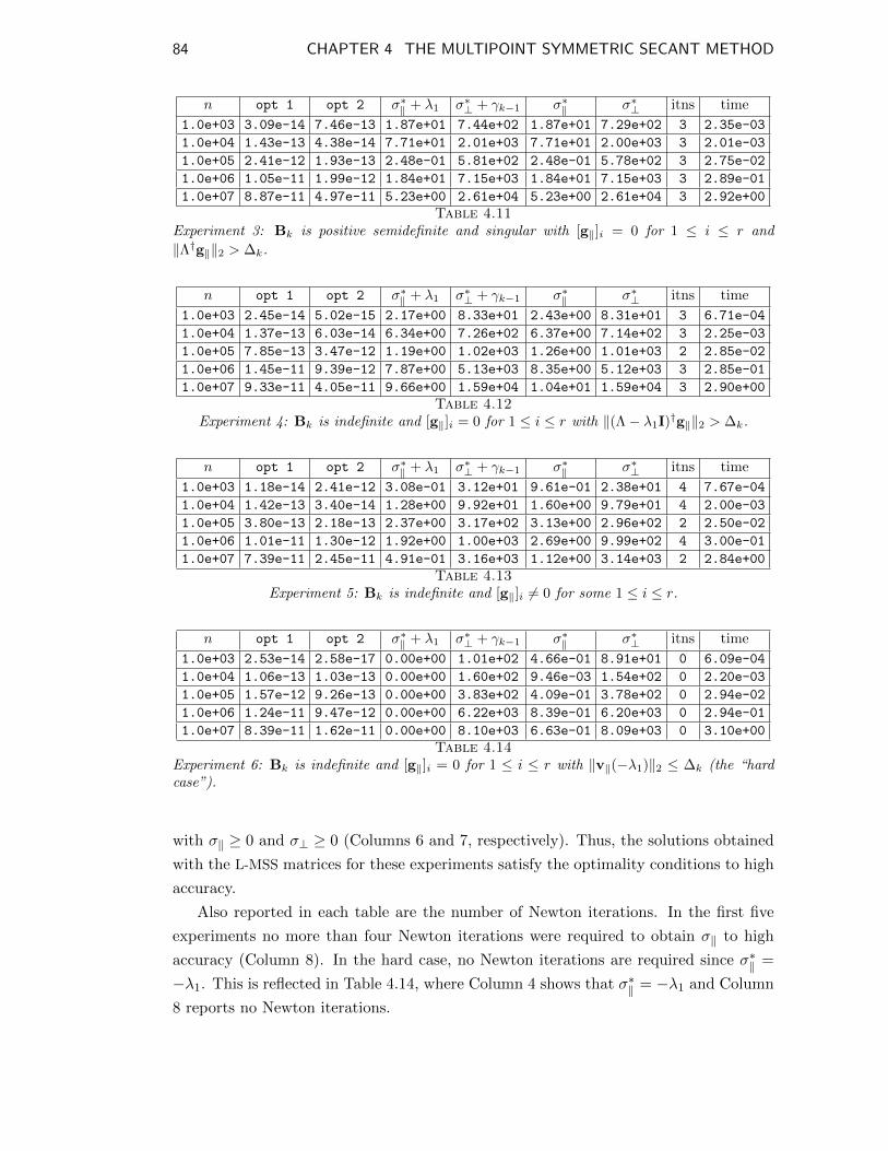
84 CHAPTER 4 THE MULTIPOINT SYMMETRIC SECANT METHOD
n opt 1 opt 2 σ∗‖ + λ1 σ∗⊥ + γk−1 σ∗‖ σ∗⊥ itns time
1.0e+03 3.09e-14 7.46e-13 1.87e+01 7.44e+02 1.87e+01 7.29e+02 3 2.35e-03
1.0e+04 1.43e-13 4.38e-14 7.71e+01 2.01e+03 7.71e+01 2.00e+03 3 2.01e-03
1.0e+05 2.41e-12 1.93e-13 2.48e-01 5.81e+02 2.48e-01 5.78e+02 3 2.75e-02
1.0e+06 1.05e-11 1.99e-12 1.84e+01 7.15e+03 1.84e+01 7.15e+03 3 2.89e-01
1.0e+07 8.87e-11 4.97e-11 5.23e+00 2.61e+04 5.23e+00 2.61e+04 3 2.92e+00
Table 4.11Experiment 3: Bk is positive semidefinite and singular with [g‖]i = 0 for 1 ≤ i ≤ r and
‖Λ†g‖‖2 > ∆k.
n opt 1 opt 2 σ∗‖ + λ1 σ∗⊥ + γk−1 σ∗‖ σ∗⊥ itns time
1.0e+03 2.45e-14 5.02e-15 2.17e+00 8.33e+01 2.43e+00 8.31e+01 3 6.71e-04
1.0e+04 1.37e-13 6.03e-14 6.34e+00 7.26e+02 6.37e+00 7.14e+02 3 2.25e-03
1.0e+05 7.85e-13 3.47e-12 1.19e+00 1.02e+03 1.26e+00 1.01e+03 2 2.85e-02
1.0e+06 1.45e-11 9.39e-12 7.87e+00 5.13e+03 8.35e+00 5.12e+03 3 2.85e-01
1.0e+07 9.33e-11 4.05e-11 9.66e+00 1.59e+04 1.04e+01 1.59e+04 3 2.90e+00
Table 4.12Experiment 4: Bk is indefinite and [g‖]i = 0 for 1 ≤ i ≤ r with ‖(Λ− λ1I)†g‖‖2 > ∆k.
n opt 1 opt 2 σ∗‖ + λ1 σ∗⊥ + γk−1 σ∗‖ σ∗⊥ itns time
1.0e+03 1.18e-14 2.41e-12 3.08e-01 3.12e+01 9.61e-01 2.38e+01 4 7.67e-04
1.0e+04 1.42e-13 3.40e-14 1.28e+00 9.92e+01 1.60e+00 9.79e+01 4 2.00e-03
1.0e+05 3.80e-13 2.18e-13 2.37e+00 3.17e+02 3.13e+00 2.96e+02 2 2.50e-02
1.0e+06 1.01e-11 1.30e-12 1.92e+00 1.00e+03 2.69e+00 9.99e+02 4 3.00e-01
1.0e+07 7.39e-11 2.45e-11 4.91e-01 3.16e+03 1.12e+00 3.14e+03 2 2.84e+00
Table 4.13Experiment 5: Bk is indefinite and [g‖]i 6= 0 for some 1 ≤ i ≤ r.
n opt 1 opt 2 σ∗‖ + λ1 σ∗⊥ + γk−1 σ∗‖ σ∗⊥ itns time
1.0e+03 2.53e-14 2.58e-17 0.00e+00 1.01e+02 4.66e-01 8.91e+01 0 6.09e-04
1.0e+04 1.06e-13 1.03e-13 0.00e+00 1.60e+02 9.46e-03 1.54e+02 0 2.20e-03
1.0e+05 1.57e-12 9.26e-13 0.00e+00 3.83e+02 4.09e-01 3.78e+02 0 2.94e-02
1.0e+06 1.24e-11 9.47e-12 0.00e+00 6.22e+03 8.39e-01 6.20e+03 0 2.94e-01
1.0e+07 8.39e-11 1.62e-11 0.00e+00 8.10e+03 6.63e-01 8.09e+03 0 3.10e+00
Table 4.14Experiment 6: Bk is indefinite and [g‖]i = 0 for 1 ≤ i ≤ r with ‖v‖(−λ1)‖2 ≤ ∆k (the “hardcase”).
with σ‖ ≥ 0 and σ⊥ ≥ 0 (Columns 6 and 7, respectively). Thus, the solutions obtained
with the L-MSS matrices for these experiments satisfy the optimality conditions to high
accuracy.
Also reported in each table are the number of Newton iterations. In the first five
experiments no more than four Newton iterations were required to obtain σ‖ to high
accuracy (Column 8). In the hard case, no Newton iterations are required since σ∗‖ =
−λ1. This is reflected in Table 4.14, where Column 4 shows that σ∗‖ = −λ1 and Column
8 reports no Newton iterations.

85 CHAPTER 4 THE MULTIPOINT SYMMETRIC SECANT METHOD
The final column reports the time required by the method to solve each subproblem.
Consistent with the best limited-memory methods, the time required to solve each
subproblem appears to grow linearly with n.
4.4.3 APPROACH II: MSSM SUBPROBLEMSWITH THE `2-NORM
Similar as in Section 4.4.3 we generated five sets of experiments composed of problems
ranging from n = 103 to n = 107. The number of limited-memory updates l was
set to 5, and thus 2l = 10. The initial matrix is a multiple of identity matrix B0 =
γk−1In with γk−1 = 0.5. The pairs Sk and Yk, both n × l matrices, were generated
from random data. Finally, gk was generated by random data and the ‘unconstrained’
minimizer is computed from the compact representation in (4.10) by the Sherman-
Morrison-Woodbury formula as su = −(γk−1In + ΨkMkΨ
Tk
)−1gk.
1. The matrix Bk is positive definite with ‖su‖2 ≤ ∆k.
2. The matrix Bk is positive definite with ‖su‖2 > ∆k.
3. The matrix Bk is positive semidefinite and singular with s = −B†kgk infeasible.
4. The matrix Bk is indefinite.
5. The hard case (Bk is indefinite): λmin = λ1 = λ1 + γk−1 < 0 and ‖(Bk −λ1In)gk)‖2 > ∆k.
We report the following: (1) opt 1 (abs)=‖(Bk+σ∗In)s∗+gk‖2, which corresponds
to the norm of the error in the first optimality conditions; (2) opt 1 (rel) =(‖(Bk +
σ∗In)s∗ + gk‖2)/‖gk‖2, which corresponds to the norm of the relative error in the first
optimality conditions; (3) opt 2=σ∗|s∗ −∆k|, which corresponds to the absolute error
in the second optimality conditions; (4) σ∗, and (5) Time. We ran each experiment five
times and report one representative result for each experiment.
Table 4.15Experiment 1: Bk is positive definite and ‖su‖2 ≤ ∆k.
n opt 1 (abs) opt 1 (rel) opt 2 σ∗ Time
1.0e+03 4.24e-15 1.34e-16 0.00e+00 0.00e+00 1.97e-03
1.0e+04 1.35e-14 1.34e-16 0.00e+00 0.00e+00 3.30e-03
1.0e+05 3.63e-14 1.15e-16 0.00e+00 0.00e+00 2.11e-02
1.0e+06 1.28e-13 1.28e-16 0.00e+00 0.00e+00 2.19e-01
1.0e+07 3.57e-13 1.13e-16 0.00e+00 0.00e+00 2.21e+00
Table 4.15 shows the results of Experiment 1. In all cases, the method found global
solutions of the trust-region subproblems.
Table 4.16 shows the results of Experiment 2. In this case, the unconstrained mini-
mizer is not inside the trust region, making the value of σ∗ strictly positive.

86 CHAPTER 4 THE MULTIPOINT SYMMETRIC SECANT METHOD
Table 4.16Experiment 2: Bk is positive definite and ‖su‖2 > ∆k.
n opt 1 (abs) opt 1 (rel) opt 2 σ∗ Time
1.0e+03 4.02e-15 1.30e-16 4.98e-15 2.99e+01 2.31e-03
1.0e+04 1.37e-14 1.35e-16 1.20e-10 1.60e+01 3.61e-03
1.0e+05 3.52e-14 1.11e-16 1.35e-12 1.65e+02 2.16e-02
1.0e+06 1.44e-13 1.44e-16 2.71e-12 1.73e+01 2.23e-01
1.0e+07 4.15e-13 1.31e-16 2.67e-11 3.69e+01 2.21e+00
Table 4.17Experiment 3: Bk is positive semidefinite and singular with ‖B†kgk‖2 > ∆k.
n opt 1 (abs) opt 1 (rel) opt 2 σ∗ Time
1.0e+03 9.88e-14 3.13e-15 6.28e-16 2.21e-02 2.26e-03
1.0e+04 3.44e-13 3.39e-15 2.45e-15 3.83e-02 3.89e-03
1.0e+05 4.10e-12 1.30e-14 5.65e-13 7.21e-03 2.13e-02
1.0e+06 1.63e-13 1.63e-16 1.91e-11 3.70e-01 2.20e-01
1.0e+07 1.14e-10 3.60e-14 6.42e-14 5.24e-04 2.20e+00
Table 4.17 displays the results of Experiment 3. In this experiment Bk is singular,
and therefore not well conditioned. The proposed method is able to obtain high accu-
racy solutions. Global solutions to the subproblems solved in Experiment 3 lie on the
boundary of the trust region.
Table 4.18Experiment 4: Bk is indefinite.
n opt 1 (abs) opt 1 (rel) opt 2 σ∗ Time
1.0e+03 1.66e-14 5.29e-16 3.72e-15 4.19e-01 2.32e-03
1.0e+04 5.33e-13 5.35e-15 8.36e-12 9.49e-01 3.76e-03
1.0e+05 4.26e-14 1.35e-16 1.77e-09 4.59e+00 2.19e-02
1.0e+06 6.64e-13 6.64e-16 1.43e-12 9.26e-01 2.25e-01
1.0e+07 4.09e-13 1.29e-16 4.52e-10 2.70e+00 2.21e+00
The results for Experiment 4 are displayed in Table 4.18. The method found solu-
tions that satisfies the first optimality condition high accuracy.
Table 4.19Experiment 5: The hard case (Bk is indefinite) and λmin = λ1 = λ1 + γk−1 < 0.
n opt 1 (abs) opt 1 (rel) opt 2 σ∗ Time
1.0e+03 9.80e-14 3.13e-15 1.16e-14 8.18e-01 2.53e-03
1.0e+04 1.66e-12 1.66e-14 1.31e-14 1.54e-01 5.25e-03
1.0e+05 1.74e-11 5.50e-14 1.66e-13 1.01e-01 4.05e-02
1.0e+06 2.76e-10 2.76e-13 2.09e-12 1.39e-01 4.64e-01
1.0e+07 1.82e-10 5.76e-14 2.34e-10 5.00e-01 4.59e+00

87 CHAPTER 4 THE MULTIPOINT SYMMETRIC SECANT METHOD
In the hard case with λmin being a nontrivial eigenvalue, the method obtains a global
solution as measured by the optimality conditions.

CHAPTER 5
LINEAR EQUALITY
CONSTRAINED
TRUST-REGION
METHODS
This chapter is based on the manuscript “Large-Scale Quasi-Newton Shape-Changing
Trust-Region Method with Low Dimensional Linear Equality Constraints” J. B. Brust,
R. F. Marcia, and C. G. Petra, which is currently in preparation.
5.1 BACKGROUND
5.1.1 PROBLEM FORMULATION
In this chapter we focus on the linear equality constraint minimization problem
minimizex∈Rn
f(x) subject to Ax = b, (5.1)
where the objective function f : Rn → R is continuously differentiable and the con-
straints are defined by A ∈ Rm×n and b ∈ Rm. We assume that m � n and that the
rectangular matrix A is of full row rank. Because it has been shown that trust-region
methods are effective for solving constrained optimization problems [CDJT84, Var85,
LNP98], we propose solving the problem in (5.1) using trust-region methods. In par-
ticular, we concentrate on trust-region methods that use limited-memory quasi-Newton
matrices, and exploit the structure of these matrices to compute the trust-region sub-
problem solutions.
88

89 CHAPTER 5 LINEAR EQUALITY CONSTRAINED TRUST-REGIONMETHODS
5.1.2 CONSTRAINED TRUST-REGION METHOD
The constrained trust-region method is obtained as an extension of the unconstrained
method described in Chapter 1, Section 1.3. Recall the quadratic subproblems of the
form
sk = arg min‖s‖≤∆k
Q(s) = sTgk +1
2sTBks (5.2)
where the solution sk is used to compute the next iterate xk+1 = xk + sk.
In order to use trust-region methods to solve (5.1), we note that if the current iterate
xk is feasible, i.e., Axk = b, then the next iterate xk+1 is also feasible, i.e., Axk+1 = b,
only if Ask = 0. Thus, the trust-region subproblem corresponding to (5.1) is given by
minimize‖s‖≤∆k
Q(s) = sTgk +1
2sTBks subject to As = 0. (5.3)
Without the equality constraint in (5.3), the trust-region subproblem can be solved
to high accuracy with the methods from Chapter 2 or using e.g. [BWX96, EM14,
BGYZ16]. However, these methods cannot be used directly to solve (5.3) with the
equality constraint.
For this chapter, the matrix Bk represents the limited-memory Broyden-Fletcher-
Goldfarb-Shanno (L-BFGS) matrix. Furthermore, we propose solving (5.3) with two
norms. Specifically, we use the shape-changing (P,∞)-norm in (2.19) from Subsec-
tion 2.5.4, as well as the `2-norm. Unlike in the previous chapters, we compute the
compact representation of part of the Hessian of the Lagrangian function (without the
norm constraint) rather than the Hessian of the objective function Q(s). This compact
representation allows Q(s) to be decomposed into two subproblems. And by using a
shape-changing norm, closed-form solutions can then be computed. We use the com-
pact representation of the inverse L-BFGS matrix Hk = B−1k in this chapter, because it
simplifies the development of our methods. In particular, let δk =yTk−1sk−1
yTk−1yk−1
, and let the
matrices Lk,Dk and Tk be as defined in Section 3.2, then the compact representation
of Hk is
Hk = δkI + ΨkMkΨTk , (5.4)
where
Mk ≡
[T−Tk (Dk + δkY
Tk Yk)T
−1k −δkT−Tk
−δkT−1k 0
],
Ψk = [ Sk Yk ] ∈ Rn×2l and with Mk ∈ R2l×2l (see [BNS94] for details). Note that
the methods that will be described in this chapter are applicable to any quasi-Newton
matrix with a compact representation, not only the L-BFGS matrix.

90 CHAPTER 5 LINEAR EQUALITY CONSTRAINED TRUST-REGIONMETHODS
5.2 LARGE-SCALE QUASI-NEWTON METHODS
5.2.1 THE KARUSH-KUHN-TUCKER (KKT) MATRIX
When the norm constraint ‖s‖ ≤ ∆k in (5.3) is not present, then the solution of this
‘unconstrained’ problem can be characterized as a stationary point of the Lagrangian
objective function
L(s, ρ) = Q(s) + ρTAs,
where ρ ∈ Rm is a vector of Lagrange multipliers. The stationary point (su, ρu) is
obtained by setting the gradient of the Lagrangian equal to zero, i.e., ∇L(su, ρu) = 0.
This gives rise to the Karush-Kuhn-Tucker (KKT) system[Bk AT
A 0
][su
ρu
]=
[−gk
0
]. (5.5)
Let K denote the KKT matrix in (5.5). Note that K can be explicitly inverted as
K−1 =
[Hk −HkA
T (AHkA)−1AHk HkAT (AHkA)−1
(HkAT (AHkA)−1)T (AHkA)−1
]≡
[K−1
11 K−112
K−121 K−1
22
].
The block-wise notation reveals that the stationary vector su = −K−111 gk depends only
on the upper left hand block, i.e. block K−111 . In the next section we will compute the
compact representation of
K−111 = Hk −HkA
T (AHkA)−1 AHk ≡ HkWk, (5.6)
where Wk = I −AT (AHkA)−1 AHk. The compact representation in (5.6) facilitates
computing the solutions to the trust-region subproblems in (5.3). Furthermore, the
compact representation enables us to develop the partial eigendecomposition of (5.6),
which we will combine with a shape-changing norm in order to compute an analytic
solution to (5.3).
5.2.2 COMPACT REPRESENTATION OF K−111
We now describe the compact representation of (5.6) with a lemma:
Lemma 5.1. The (1,1) block of the inverse KKT matrix in (5.6) has the compact
representation
K−111 = δkI + ΨkMkΨ
Tk , (5.7)
where
Ψk ≡ [AT Ψk], Mk ≡ −
[M11 M12
MT12 M22
], Kk = AΨkMk,

91 CHAPTER 5 LINEAR EQUALITY CONSTRAINED TRUST-REGIONMETHODS
and where
M11 = δ2k(AHkA
T )−1, M12 = δ−1k M11Kk, M22 = δ−2
k KTkM11Kk − Mk.
Proof. Define Kk ≡ AΨkMk, and observe that
AHk = δkA + AΨkMkΨTk ≡ δkA + KkΨ
Tk = [δkIm Kk]
[A
ΨTk
].
Now let M11 ≡ δ2k(AHkA
T )−1, so that
HkAT (AHkA
T )−1AHk = [AT Ψk]
[M11 δ−1
k M11Kk
δ−1k KT
kM11 δ−2k KT
kM11Kk
][A
ΨTk
].
Next, expressing Hk, from (5.4), as
Hk = δkI + ΨkMkΨTk = δkI + [AT Ψk]
[0m
Mk
][An
ΨTk
],
and combining the previous identities, yields
K−111 = Hk −HkA
T (AHkA)−1 AHk
= δkI− [AT Ψk]
[M11 M12
MT12 M22
][An
ΨTk
]≡ δkI + ΨkMkΨ
Tk ,
where M12 ≡ δ−1k M11Kk, M22 ≡ δ−2
k KTkM11Kk − Mk, and where Ψk and Mk are
defined so that the last equivalence holds. �
5.3 TRUST-REGION APPROACH WITH AN `2 CON-
STRAINT
If the `2-norm is used in (5.3), that is, ‖s‖2 ≤ ∆k is used, then the solution, defined by
the optimal Lagrange multiplier σ∗ ≥ 0 and a vector of Lagrange multipliers ρ∗, is the
vector s∗ that satisfies the system[(Bk + σ∗I) AT
A 0
][s∗
ρ∗
]=
[−gk
0
]. (5.8)

92 CHAPTER 5 LINEAR EQUALITY CONSTRAINED TRUST-REGIONMETHODS
In solving this latter system, we express the optimal vectors s∗ ≡ s∗(σ∗) as:
s∗(σ∗) = −(Bk + σ∗I)−1(I−AT
(A(Bk + σ∗I)−1AT
)−1A(Bk + σ∗I)−1
)gk
= −H∗kW∗kgk, (5.9)
where H∗k = (Bk + σ∗I)−1, and W∗k = I −AT
(A(Bk + σ∗I)−1AT
)−1A(Bk + σ∗I)−1.
When an arbitrary σ is used, instead of the optimal σ∗, we use the expression s(σ) =
HkWkgk to represent (5.9). Now, if ‖s(0)‖2 ≤ ∆k, then the expression in (5.9) with
σ∗ = 0, yields the subproblem solution. Otherwise we use Newton’s method to solve for
σ∗ > 0 in the so-called secular-equation [CGT00]
φ(σ∗) =1
‖s∗(σ∗)‖2− 1
∆k= 0. (5.10)
The solution of the latter scalar equation corresponds to ‖s∗(σ∗)‖2 = ∆k. First note
thatd
dσ(φ(σ)) = φ′(σ) = − s(σ)T s′(σ)
‖s(σ)‖32,
where s′(σ) represents the derivative of s(σ). The vector s′(σ) is computed by differen-
tiating both sides of the system in (5.8), i.e.,
d
dσ
([(Bk + σI) AT
A 0
][s
ρ
])=
d
dσ
([−gk
0
]),
and subsequently solving the resulting equations for s′:[(Bk + σI) AT
A 0
][s′
ρ′
]=
[−s(σ)
0
].
The expression for s′ ≡ s′(σ) is
s′(σ) = −(Bk + σI)−1(I−AT
(A(Bk + σI)−1AT
)−1A(Bk + σI)−1
)s(σ)
= −HkWks(σ).
Now observe that the matrix HkWk is symmetric positive semidefinite for positive
values of σ, so that
−s(σ)T s′(σ) = s(σ)T HkWks(σ) ≥ 0
for σ ≥ 0. This implies that φ′(σ) ≥ 0 for σ ≥ 0. In other words, φ(σ) is monotonically
increasing for positive σ. Because Newton’s method is applied in the case that ‖s(0)‖2 =
‖s(0)‖2 ≥ ∆k, corresponding to φ(0) < 0, a unique σ∗ > 0 can be computed that solves
the secular-equation in (5.10).

93 CHAPTER 5 LINEAR EQUALITY CONSTRAINED TRUST-REGIONMETHODS
The algorithms developed in this article assume that a feasible initial point x0 ∈ Rn
is given. The approach with a `2 norm is summarized in Algorithm 5.1
ALGORITHM 5.1:
1. Initialization: ∆0 > 0,0 ≤ d− ≤ 1 ≤ d+, δ0 = 1/‖Wg0‖2, Ψ0 = AT , M0 =
δ0(AAT )−1, B0 = In, k = 0;
2. Set: sk = −(δkI−ΨkMkΨ
Tk
)gk;
3. If ‖sk‖2 ≤ ∆k and f(xk + sk) < f(xk) then go to 6. otherwise go to 4.;
4. Set sk = s∗(eq.(5.9));
5. If f(xk + sk) < f(xk) then go to 6., otherwise ∆k = d−∆k go to 4.;
6. Set ∆k = d+∆k, xk = xk + sk, update Ψk,Mk,Bk,gk, δk, k = k + 1 go to 2.;
5.4 TRUST-REGION APPROACH WITH A SHAPE-
CHANGING CONSTRAINT
Instead of the `2-norm, we will next describe how to apply a shape-changing norm
in the context of a constrained trust-region method. First, we use a transformation
based on the eigenvectors of the (1,1) block of the inverse KKT matrix from (5.6), in
order to simplify the trust-region subproblem. Then we propose an effective method
to obtain the eigendecomposition of the relevant KKT block. Finally, we decouple the
transformed trust-region subproblem by applying a shape-changing norm, and compute
analytic solutions.
5.4.1 TRANSFORMATION OF THE TRUST-REGION SUBPROB-
LEM
In this subsection we transform the quadratic objective function from (5.3), by a change
of variables. The transformed objective can then be combined with a shape-changing-
norm, to effectively solve the subproblem. Observe that the nullspace of K−111 is spanned
by the columns of AT , i.e. K−111 AT = 0. Therefore, the eigendecomposition of K−1
11 can
be represented as
K−111 = PΛPT = [P‖1 P2]
[0m
Λ−12
][P‖1 P2]T , (5.11)
where the orthonormal eigenvectors are contained in the matrix P = [P‖1 P2] ∈ Rn×n
(I = PPT = PTP ), and where Λ−12 ∈ R(n−m)×(n−m) symbolizes a diagonal matrix

94 CHAPTER 5 LINEAR EQUALITY CONSTRAINED TRUST-REGIONMETHODS
of eigenvalues. In this notation the rectangular matrix P‖1 ∈ Rn×m represents the
eigenvectors corresponding to the zero eigenvalues of K−111 . With this, we deduce, since
AT ∈ Range(P‖1
), the following identity: PT
2 AT = 0(n−m)×m. In order to diagonalize
and to decouple the subproblem in (5.3), we first propose Lemma 1 that describes the
relation between the eigenvectors in the rectangular matrix P2 ∈ Rn×(n−m) and the
quasi-Newton matrix Bk.
Lemma 5.2. The identity PT2 BkP2 = Λ2 holds for the eigenvectors and eigenvalues
from (5.11).
Proof. Multiply the (1,1) block of KK−1 by PT2 from the left and by P2 from the right,
so that:
PT2 [In 0n×m]KK−1
[In
0m×n
]P2 = PT
2
(BkK
−111 + ATK−1
21
)P2
= PT2
(BkPΛPT + ATK−1
21
)P2
= PT2 BkP2Λ
−12 .
Now, since KK−1 = In+m, and since the matrix P2 has orthonormal columns, it holds
that
PT2 BkP2Λ
−12 = In−m.
Therefore we conclude that PT2 BkP2 = Λ2. �
To diagonalize the constrained subproblem we apply the change of variables v =[v‖1v2
]=
[PT‖1s
PT2 s
]= PT s. First, we analyze the effect of this change on the linear
constraints:
As = APv = [AP‖1 0m×(n−m)]v = AP‖1v‖1 = 0.
Since AT is in the range of P‖1, we may represent AT as AT = P‖1R1 with an m×minvertible matrix R1. Thus the constraint
AP‖1v‖1 =(RT
1 PT‖1
)P‖1v‖1 = RT
1 v‖1 = 0,
implies that v‖1 = 0. Second, we examine the effect of the change of variables on the
quadratic approximation Q(s):
Q(s) = Q(Pv) = gTk (Pv) +1
2vTPTBkPv
= gTk (P2v2) +1
2vT2 PT
2 BkP2v2
= gTk (P2v2) +1
2vT2 Λ2v2
≡ q(v2),

95 CHAPTER 5 LINEAR EQUALITY CONSTRAINED TRUST-REGIONMETHODS
where we apply Lemma 5.2 to obtain the last equality. Observe that Q(Pv) ≡ q(v2) is
an quadratic objective function defined by the diagonal matrix of eigenvalues Λ2 and by
the n −m unknowns denoted as v2. Because the matrix in the transformed quadratic
objective function is diagonal, it will be straightforward to later separate it into different
subspaces. Since the change of variables relies on the eigendecomposition of the matrix
K−111 , we first develop an effective partial eigenfactorization of K−1
11 .
5.4.2 PARTIAL EIGENDECOMPOSITION OF K−111
Our approach to computing the eidendecomposition of (5.7) is based on factoring the
low rank matrix Uk ≡ ΨkMkΨTk . Note that since Rank(Uk) = 2l +m, the matrix Uk
has only 2l+m non-zero eigenvalues. We denote the orthonormal basis that corresponds
to the nullspace of Uk as P⊥ ∈ Rn×(n−(2l+m)). In other words, the matrix P⊥ satisfies
UkP⊥ = 0. However, since the matrix P⊥ would be prohibitively expensive to compute
when n becomes large, we do not explicitly compute it in our approach. Next observe,
from e.g. (5.6), that K−111 AT = (δkI−Uk)A
T = 0 so that UkAT = δkA
T . Therefore the
set of eigenvectors of Uk, corresponding to the repeated eigenvalue δk, can be expressed
as P‖1 = AT (AAT )−1/2. We thus represent the factorization of Uk as
Uk = [AT Ψk]Mk
[A
ΨTk
]= [P‖1 P‖2 P⊥]
δkIm
D−12
0
PT‖1
PT‖2
PT⊥
, (5.12)
where D−12 ∈ R2l×2l is a diagonal matrix of eigenvalues, and the columns of the rect-
angular matrices P‖1 ∈ Rn×m, P‖2 ∈ Rn×2l, P⊥ ∈ Rn×(n−(2l+m)) represent mutually
orthogonal eigenvectors. Next we describe how to compute the non-zero eigenvalues in
the matrix D−12 and its corresponding eigenvectors in P‖2. Subsequently, we combine
the results to arrive at the implicit eigendecomposition of (5.7). First, deflate the right
hand side in (5.12), by substituting P‖1 = AT (AAT )−1/2, and by suppressing the zero
eigenvalues. In this way we obtain an identity for the eigenvectors P‖2 and eigenvalues
D−12 :
[AT Ψk]
[M11 −
(AAT
)−1M12
MT12 M22
][A
ΨTk
]= P‖2D
−12 PT
‖2. (5.13)
Since 0 = PT‖1P‖2 = (AAT )−1/2AP‖2, which means that AP‖2 = 0, then we apply the
orthogonal projection W = I −AT (AAT )−1A from the left and from the right to the
expression in (5.13), so that
WΨkM22ΨTkWT = P‖2D
−12 PT
‖2.

96 CHAPTER 5 LINEAR EQUALITY CONSTRAINED TRUST-REGIONMETHODS
Next compute the non-zero eigenvalues of WΨkM22ΨTkWT using an implicit QR fac-
torization of the matrix WΨk ∈ Rn×2l. In particular, let WΨk = QR where we do not
explicitly compute the orthogonal matrix Q ∈ Rn×2l, and where R ∈ R2l×2l is an up-
per triangular matrix. Then we explicitly compute the eigendecomposition of the small
matrix RM22RT = VD−1
2 VT , where V ∈ R2l×2l is orthogonal and D−12 is a diagonal
matrix of eigenvalues. With this
WΨkM22ΨTkWT = QRM22R
TQT = QVD−12 RTVT .
Now, since QV is a matrix of orthonormal columns, and D−12 is diagonal we find that
QV = P‖2 and D−12 = D−1
2 . Note that Q is not explicitly computed, instead we
represent it with the identity QR = WΨk as Q = WΨkR−1. Thus P‖2 has the
explicit form
P‖2 = QV = WΨkR−1V =
(Ψk −AT (AAT )−1AΨk
)R−1V.
To compute the upper triangular matrix R we set R = LD1/2, where we compute the
LDLT factorization (WΨk)TWΨk = (QR)TQR = LDLT . Based on the previous
analysis we now obtain the implicit eigendecomposition of K−111 from (5.7). Since the
columns of P = [P‖1 P‖2 P⊥] ∈ Rn×n are mutually orthogonal, we obtain the factor-
ization
K−111 = δkI− [AT Ψk]
[M11 M12
MT12 M22
][A
ΨTk
]
= δkI− [P‖1 P‖2 P⊥]
δkIm
D−12
0
PT‖1
PT‖2
PT⊥
= [P‖1 P‖2 P⊥]
0m
δkI2l −D−12
δkIn−(2l+m)
PT‖1
PT‖2
PT⊥
, (5.14)
where
P‖1 = AT (AAT )−1/2, P‖2 =(Ψk −AT (AAT )−1AΨk
)R−1V, D−1
2 = D−12 .
Observe that the eigendecomposition only requires the computation of a few eigenvalues
(2l), corresponding to (δkI2l−D−12 ) explicitly. Moreover, we do not compute the columns
of the matrix P⊥ explicitly.

97 CHAPTER 5 LINEAR EQUALITY CONSTRAINED TRUST-REGIONMETHODS
5.4.3 SOLVING THE SHAPE-CHANGING SUBPROBLEM
This subsection describes the solution to the subproblem in (5.3), with the shape-
changing (P,∞)-norm:
‖s‖P,∞ ≡ max(∥∥v‖∥∥∞ , ‖v⊥‖2) . (5.15)
Here we define v‖ = PT‖ s =
[PT‖1s
PT‖2s
]=
[v‖1v‖2
], and v⊥ = PT
⊥s. Then, using the change
of variable s = Pv, the original minimization has an equivalent expression
minimize‖s‖P,∞ ≤ ∆k
As = 0
Q(s) = minimize‖Pv‖P,∞ ≤ ∆k
v‖1 = 0
Q(Pv).
The objective function Q(Pv) and the shape-changing norm now further decouple. First
recall, from Subsection 5.4.1, that Q(Pv) = q(v2). Then, denoting P2 = [P‖1 P‖2],
we define the vectors PT2 gk ≡
[PT‖2gk
PT⊥gk
]=
[g‖2g⊥
], and v2 ≡
[ v‖2v⊥
]. With the notation
Λ2 =
[(δkI−D−1
2 )−1
γkI
]≡[
Λ2γkI
], and the result of Lemma 5.2, then Q(Pv) separates
once more:
Q(Pv) = q(v2) = gTk (P2v2) +1
2vT2 PT
2 BkP2v2
= gT‖2v‖2 + gT⊥v⊥ +1
2
(vT‖2Λ2v‖2 + γk ‖v⊥‖22
).
In other words, the objective function can be further decoupled into the variables v‖2
and v⊥. Simultaneously, the shape-changing constraint also decouples into v‖2 and v⊥.
Since v‖1 = 0, then the norm constraint satisfies the equivalence relation:
max(∥∥v‖∥∥∞ , ‖v⊥‖2) ≤ ∆k is equivalent to max
(∥∥v‖2∥∥∞ , ‖v⊥‖2) ≤ ∆k.
Using our analysis, the minimization of the subproblem (5.3) with the shape-changing
norm as defined in (5.15), is equivalent to the minimization of two decoupled diagonal-
ized problems
minimize‖v‖2‖∞≤∆k
gT‖2v‖2 +1
2vT‖2Λ2v‖2 + minimize
‖v⊥‖2≤∆k
gT⊥v⊥ +γk2‖v⊥‖22 .

98 CHAPTER 5 LINEAR EQUALITY CONSTRAINED TRUST-REGIONMETHODS
The two separated minimization problems can be solved analytically. Specifically, letting
λi ≡ [Λ2]ii = [(δkI− D−12 )−1]ii, then the solution of v∗‖2 is given, coordinate-wise, by
[v∗‖2]i =
− [g‖2]iλi
if
∣∣∣∣ [g‖2]iλi
∣∣∣∣ ≤ ∆k and λi > 0,
c if[g‖2]i
= 0 and λi = 0,
−sgn([g‖2]i)∆k if
[g‖2]i6= 0 and λi = 0,
±∆k if[g‖2]i
= 0 and λi < 0,
− ∆k
|[g‖2]i|[g‖2]i
otherwise,
, (5.16)
where c is any real number in [−∆k,∆k] and ‘sgn’ denotes the signum function. The
minimizer v∗⊥ is given by
v∗⊥ = βg⊥, (5.17)
where
β =
−δk if δk > 0 and ‖δkg⊥‖2 ≤ ∆k,
− ∆k‖g⊥‖2 otherwise.
(5.18)
Thus, v∗ =
0
v∗‖2v∗⊥
, yields the solution s∗, by using the transformation s∗ = Pv∗. Since
our method does not compute the large orthonormal matrix P⊥, the next subsection
describes a direct formula to compute s∗.
5.4.4 COMPUTING THE SOLUTION s∗
Observe that since P = [P‖1 P‖2 P⊥] is orthogonal, then PPT = P‖1PT‖1 + P‖2P
T‖2 +
P⊥PT⊥ = In. Therefore, P⊥PT
⊥ = In−P‖1PT‖1−P‖2P
T‖2 and the previous computations,
yield
s∗ = Pv∗
= [P‖1 P‖2 P⊥]
0
v∗‖2v∗⊥
= P‖2v
∗‖2 + P⊥v∗⊥
= P‖2v∗‖2 + βP⊥PT
⊥gk
= P‖2
(v∗‖2 − βg‖2
)+ β
(In −AT
(AAT
)−1A)
gk. (5.19)
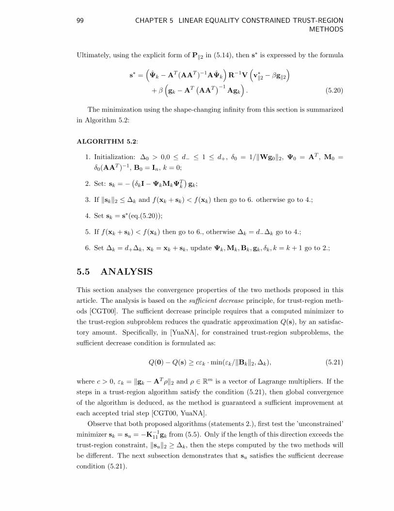
99 CHAPTER 5 LINEAR EQUALITY CONSTRAINED TRUST-REGIONMETHODS
Ultimately, using the explicit form of P‖2 in (5.14), then s∗ is expressed by the formula
s∗ =(Ψk −AT (AAT )−1AΨk
)R−1V
(v∗‖2 − βg‖2
)+ β
(gk −AT
(AAT
)−1Agk
). (5.20)
The minimization using the shape-changing infinity from this section is summarized
in Algorithm 5.2:
ALGORITHM 5.2:
1. Initialization: ∆0 > 0,0 ≤ d− ≤ 1 ≤ d+, δ0 = 1/‖Wg0‖2, Ψ0 = AT , M0 =
δ0(AAT )−1, B0 = In, k = 0;
2. Set: sk = −(δkI−ΨkMkΨ
Tk
)gk;
3. If ‖sk‖2 ≤ ∆k and f(xk + sk) < f(xk) then go to 6. otherwise go to 4.;
4. Set sk = s∗(eq.(5.20));
5. If f(xk + sk) < f(xk) then go to 6., otherwise ∆k = d−∆k go to 4.;
6. Set ∆k = d+∆k, xk = xk + sk, update Ψk,Mk,Bk,gk, δk, k = k + 1 go to 2.;
5.5 ANALYSIS
This section analyses the convergence properties of the two methods proposed in this
article. The analysis is based on the sufficient decrease principle, for trust-region meth-
ods [CGT00]. The sufficient decrease principle requires that a computed minimizer to
the trust-region subproblem reduces the quadratic approximation Q(s), by an satisfac-
tory amount. Specifically, in [YuaNA], for constrained trust-region subproblems, the
sufficient decrease condition is formulated as:
Q(0)−Q(s) ≥ cεk ·min(εk/‖Bk‖2,∆k), (5.21)
where c > 0, εk = ‖gk −ATρ‖2 and ρ ∈ Rm is a vector of Lagrange multipliers. If the
steps in a trust-region algorithm satisfy the condition (5.21), then global convergence
of the algorithm is deduced, as the method is guaranteed a sufficient improvement at
each accepted trial step [CGT00, YuaNA].
Observe that both proposed algorithms (statements 2.), first test the ’unconstrained’
minimizer sk = su = −K−111 gk from (5.5). Only if the length of this direction exceeds the
trust-region constraint, ‖su‖2 ≥ ∆k, then the steps computed by the two methods will
be different. The next subsection demonstrates that su satisfies the sufficient decrease
condition (5.21).

100 CHAPTER 5 LINEAR EQUALITY CONSTRAINED TRUST-REGIONMETHODS
5.5.1 SUFFICIENT DECREASE WITH THE ‘UNCONSTRAINED’
MINIMIZER su
First observe, from the definition of Wk in (5.6), that WTk HkWk = HkWk. Then
substitute the unconstrained minimizer, sk = su = −K−111 gk = −HkWkgk into the left
hand side of (5.21), to obtain
Q(0)−Q(sk) = gTk HkWkgk − 1/2gTk WTk HkWkgk
= 1/2gTk WTk HkWkgk
≥ 1
2λmax
gTk WTk Wkgk
≡ 1/2(εuk)2
‖Bk‖2= 1/2εuk ·min(εuk/‖Bk‖2,∆k), (5.22)
where εuk = ‖Wkgk‖2 = ‖gk −ATρu‖2 and where ρu is specified by the system in (5.5).
Comparing the last equality from (5.22) with (5.21), we conclude that the unconstrained
minimizer satisfies the sufficient decrease condition.
5.5.2 SUFFICIENT DECREASE WITH THE `2 CONSTRAINT
In Algorithm 5.1, with the `2 constraint the search direction is computed as
s∗k = −H∗kW∗kgk = −(Bk + σ∗I)−1W∗
kgk,
where W∗k is as defined below (5.9). Next it is demonstrated that s∗k satisfies the
sufficient decrease condition. In particular, we propose
Lemma 5.3. The solution
s∗k = −(Bk + σ∗In)−1(I−AT
(A(Bk + σ∗In)−1AT
)−1A(Bk + σ∗In)−1
)gk
where σ∗ ≥ 0, of the trust-region subproblem in (5.2) defined by the `2-norm satisfies
the sufficient decrease condition from (5.21).
Proof. First, when σ∗ = 0 then s∗k = su, so that the sufficient decrease condition is as
in (5.22). If σ∗ > 0, then s∗k lies on the boundary, i.e. ‖s∗k‖2 = ∆k. In this case, observe
that
(s∗k)T (Bk + σ∗I)s∗k = (s∗k)
TBksk + σ∗∆2k = −(s∗k)
TW∗kgk = gTk (W∗
k)T H∗kW
∗kgk.

101 CHAPTER 5 LINEAR EQUALITY CONSTRAINED TRUST-REGIONMETHODS
Moreover, from the definition of W∗k, it holds that (W∗
k)T H∗kW
∗k = H∗kW
∗k. Therefore
Q(0)−Q(s∗k) = −(gTk s∗k + 1/2(s∗k)TBks
∗k)
= −(gTk s∗k + 1/2(gTk (W∗
k)T H∗kW
∗kgk − 1/2σ∗∆2
k))
= −(−gTk H∗kW
∗kgk + 1/2(gTk (W∗
k)T H∗kW
∗kgk − 1/2σ∗∆2
k))
= 1/2gTk (W∗k)T H∗kW
∗kgk + 1/2σ∗∆2
k.
Since H∗k = (Bk + σ∗I)−1 we deduce that‖W∗
kgk‖22λmax+σ∗
≤ gTk (W∗k)T H∗kW
∗kgk. Moreover
since
∆2k = (s∗k)
T s∗k = gTk (W∗k)T (H∗k)
2W∗kgk ≤
‖W∗kgk‖22
(λmin + σ∗)2,
an upper bound on σ∗ is: σ∗ ≤ ‖W∗kgk‖2∆k
. Letting εlk = ‖W∗kgk‖2 = ‖gk − AT ρ∗‖2,
where ρ∗ is specified by the system in (5.8), then the inequalities hold
Q(0)−Q(sk) = 1/2gTk (W∗k)T H∗kW
∗kgk + 1/2σ∗∆2
k
≥ 1/2gTk (W∗k)T H∗kW
∗kgk
≥ 1/2
((εlk)
2
λmax + σ∗
)≥ 1/2
((εlk)
2
‖Bk‖2 + εlk∆−1k
).
Now consider two cases. Case 1 is defined by the condition ‖Bk‖2 > εlk∆−1k , which
means that Q(0)−Q(sk) ≥ 1/4 · (εlk)2/‖Bk‖2. Case 2 is defined when ‖Bk‖2 < εlk∆−1k ,
which means that Q(0)−Q(sk) ≥ 1/4 · εlk∆k. Therefore we conclude that the sufficient
decrease condition of (5.21), with the `2 constraint, holds as:
Q(0)−Q(sk) ≥ 1/4εlk ·min(εlk/‖Bk‖2,∆k),
where εlk = ‖gk −AT ρ∗‖2. �
5.5.3 SUFFICIENT DECREASE WITH THE SHAPE-CHANGING
CONSTRAINT
Note from Section 5.4.1 that the quadratic objective function has an equivalent repre-
sentation in a transformed space, i.e. Q(s) = q(v2). This relation connects the sufficient
decrease condition in the transformed space to the same condition in the original space.
Lemma 5.4. The solution
s∗ = Pv∗ = P
[0
v∗2
],

102 CHAPTER 5 LINEAR EQUALITY CONSTRAINED TRUST-REGIONMETHODS
in (5.19) to the trust-region subproblem in (5.3) defined by the shape-changing norm
(5.15), satisfies the sufficient decrease condition (5.21).
Proof. Represent
v∗2 = −
θ1,1
. . .
θ2l,2l
βIn−(m+2l)
g2 ≡ −Θ2g2,
where
θi,i =
1λi
if
∣∣∣∣ [g‖2]iλi
∣∣∣∣ ≤ ∆k
−∆k[g‖2]i|[g‖2]i|
otherwise,
and where β is as defined in (5.18). Observe that the component-wise inequality Θ2Λ2 ≤I holds. Thus
Q(0)−Q(s∗) = −q(v∗2) = −(
gT2 v∗2 +1
2(v∗2)TΛ2v
∗2
)= −
(−gT2 Θ2g2 +
1
2gT2 Θ2Λ2Θ2g2
)≥ 1
2gT2 Θ2g2
≥ 1
2gT2 g2min (1/λmax,∆k/‖g2‖2)
=1
2‖g2‖2min (‖g2‖2/‖Λ2‖2,∆k) .
Moreover,
‖g2‖22 = gTk P2PT2 gk = ‖(I−AT (AAT )−1A)gk‖22 ≡ ‖gk −ATρPk ‖22,
where ρPk ≡ (AAT )−1Agk. Since PT2 BkP2 = Λ2 and therefore ‖Bk‖2 ≥ ‖Λ2‖2, the
sufficient decrease condition from (5.21) holds as
Q(0)−Q(s∗) = −q(v∗2) ≥ 1/2‖g2‖2min (‖g2‖2/‖Λ2‖2,∆k)
≥ 1/2εPk ·min(εPk /‖Bk‖2,∆k
),
where εPk = ‖gk −ATρPk ‖2. �
5.5.4 CONVERGENCE
The convergence of algorithms 5.1 and 5.2 will be established in a theorem, which invokes
the theory developed by Conn et al. [CGT00]. To be consistent with [CGT00], our

103 CHAPTER 5 LINEAR EQUALITY CONSTRAINED TRUST-REGIONMETHODS
result is based on the assumptions: A. The objective function f(x) is twice continuously
differentiable, it is bounded from below (f(x) ≥ k−), and the Hessian is bounded from
above (∇2f(x) ≤ k+). B. The constraints are twice continuously differentiable, and they
are consistent. C. A first order constraint qualification holds at a stationary point x∗.
D. The quadratic approximation Q(s) is twice continuously differentiable, and E. The
quasi-Newton matrix Bk is invertible for all k, i.e., the lowest eigenvalue λmin is bounded
from 0, and the largest eigenvalue λmax is bounded from infinity. These properties are
shown for the L-BFGS matrix in [BGYZ16]. Finally we note that
1√l +m
‖s‖2 ≤ ‖s‖P,∞ ≤√l +m‖s‖2,
which relates the shape-changing norm to the `2-norm (cf. Section 2.5.4), and ensures
a measure of ‘closeness’ to the `2-norm . We thus propose
Theorem 5.5. Suppose that the eigenvalues of Bk are bounded, i.e., 0 < cl ≤ λmin ≤λmax < cu for some constants cl and cu. Then every limit point of the sequence of iterates
xk,xk+1, . . . generated by algorithm 5.1, or by algorithm 5.2, is first order critical.
Proof. The algorithms proposed in this section have the same form as Algorithm 12.2.1
p. 452 [CGT00], which is included here for completeness. Note that the algorithm is
reproduced almost literally, except for slight adaptations in order to be consistent with
the problem formulation of this chapter.
ALGORITHM 5.3 (Algorithm 12.2.1 in [CGT00])
Step 0: Initialization. An initial feasible point x0 and an initial trust-region radius
∆0 are given. The constants 0 < ε1 ≤ ε2 < 1 and 0 < γ1 ≤ γ2 < 1 are also given.
Compute f(x0) and set k = 0.
Step 1: Model definition. Define a model Q(s) subject to As = 0, ‖s‖ ≤ ∆k.
Step 2: Step calculation. Compute a step sk that sufficiently reduces the modelQ(s)
in the sense of (5.23) and (5.24), while sk satisfies the constraints from Step 1;
Step 3: Acceptance of the trial point. Compute f(xk + sk) and define the ratio
ρk =f(xk)− f(xk + sk)
Q(0)−Q(sk).
If ρk ≥ ε1, then define xk+1 = xk + sk; otherwise define xk+1 = xk.

104 CHAPTER 5 LINEAR EQUALITY CONSTRAINED TRUST-REGIONMETHODS
Step 4: Trust-region radius update. Set
∆k+1 ∈
[∆k,∞) if ρk ≥ ε2,
[γ2∆k,∆k] if ρk ∈ [ε1, ε2),
[γ1∆k, γ2∆k] if ρk < ε1.
Increment k by 1 and go to Step 1.
Algorithm 12.2.1 converges to a first order critical point, as long as the steps sk
satisfy the sufficient-decrease condition
Q(0)−Q(sk) ≥ cπkmin (πk/‖Bk‖2,∆k) , (5.23)
where 0 < c < 1, and
πk =
∣∣∣∣ minimize‖s‖2≤1
gTk s
∣∣∣∣ subject to As = 0. (5.24)
Observe that by solving the minimization in (5.24) that πk is expressed as
πk =∥∥(In −AT (AAT )−1A)gk
∥∥2
= εPk ,
where εPk is as specified in the proof of lemma 5.4. Therefore we conclude that algorithm
5.2 satisfies the sufficient decrease condition (5.23), and consequently converges to a
critical point. In the `2-norm algorithm we have
εlk =∥∥gk −AT ρ∗
∥∥2
=∥∥(In −AT (A(Bk + σ∗In)−1AT )−1(A(Bk + σ∗In)−1)gk
∥∥2
≥ λmin + σ∗
λmax + σ∗
∥∥(In −AT (AAT )−1A)gk∥∥
2
=λmin + σ∗
λmax + σ∗πk.
By assumption there exist two positive constants cl and cu, so that 0 < cl ≤ λmin ≤λmax < cu and thus
εlk ≥ cl/cuπk,
where cl/cu ≥ 1. Therefore we conclude that algorithm 5.1 also satisfies (5.23), and
thus converges to a critical point. �

105 CHAPTER 5 LINEAR EQUALITY CONSTRAINED TRUST-REGIONMETHODS
5.6 NUMERICAL EXPERIMENTS
This section describes numerical experiments of comparing the two methods that we
developed in this article, namely Algorithms 1 and 2, which we label as TR–`2 and
TR–(P,∞), respectively. We perform four sets of experiments. In Experiment I, we
generated synthetic convex quadratic problems with linear equality constraints as test
problems. In Experiment II, we considered problems from CUTEst with linear con-
straints. Among the selected linear problems we filter for the ones that have fewer con-
straints than unknowns. Even though many of the problems selected in this way include
inequality and bound constraints, the test is are carried out as if all constraints were
equality constraints. In Experiment III, we use 62 large-scale unconstrained CUTEst
problems, and impose synthetically generated linear equality constraints on the un-
constrained problems. The fourth part applies extensions of our methods in order to
solve a nonlinearly constraint problem. Performance profiles (see [DM02]) are provided,
when they yield additional insights. In particular, we compare the number of iterations
(iter) (when the trust-region step is accepted) and the average time (time) for each
solver on the test set of problems. The performance metric, ρ, with a given number of
test problems, np, is
ρs(τ) =card {p : πp,s ≤ τ}
npand πp,s =
tp,smin tp,i1≤i≤S
,
where tp,s is the “output” (i.e., time or iterations) of “solver” s on problem p. Here S
denotes the total number of solvers for a given comparison. This metric measures the
proportion of how close a given solver is to the best result. Throughout this section,
the two proposed algorithms are regarded to have converged when two conditions are
simultaneously satisfied:
∥∥gk −AT (AAT )−1Agk∥∥
2≤ ε1max (1, ‖xk‖2) and ‖Axk − b‖2 ≤ ε2.
Typically we set ε1 = 1 × 10⁻³ and ε2 = 1 × 10⁻⁵. Other parameters in the algorithm
are d− = 1/4, d+ = 2 and l = 5. The implementations and tests are carried out in
MATLAB.
5.6.1 EXPERIMENT I
The purpose of this experiment is to test the convergence properties of the algorithms,
and to compare their performances as the problem dimension n varies. In particular,
we randomly generate the problem data
Q ∈ Rn×n, g ∈ Rn, A ∈ Rm×n, b ∈ Rm,

106 CHAPTER 5 LINEAR EQUALITY CONSTRAINED TRUST-REGIONMETHODS
where the matrix Q is positive semidefinite, and where we define the objective functions
as f(x) = gTx+1/2xTQx. We setm = 10 and vary n ∈ {20, 50, 100, 1000, 5000, 7000, 10000}.The results of running the two methods are summarized in Fig. 5.1:
1 1.05 1.1 1.15 1.2
0.6
0.7
0.8
0.9
1
τ
ρs(τ
)
TR-(P,∞)TR-ℓ2
1 1.05 1.1 1.15 1.2 1.25
0.4
0.5
0.6
0.7
0.8
0.9
1
τ
ρs(τ
)
TR-(P,∞)TR-ℓ2
Figure 5.1 Performance profiles comparing iter (left) and time (right) of applying TR–`2 andTR–(P,∞) on convex quadratic problems with varying dimension sizes.
We observe that both solvers converge on all test problems, and that TR–(P,∞)
performs well in terms of time and iterations.
5.6.2 EXPERIMENT II
The purpose of this experiment is to apply our algorithms to a set of standard test
problems that are of the form (5.1). In this context, we filter the CUTEst library
for problems with linear constraints, and dimensions of the form 1 ≤ m ≤ 200 and
201 ≤ n < ∞. Among the problems that are selected, using the above search criteria,
many include linear inequality constraints, or bounds on the variables. In our tests we
treat all inequalities as equality constraints, and do not attempt to satisfy the bounds.
The selected problems are
We report whether a algorithm converged on a particular problem (conv), the num-
ber of function evaluation it required (fval) and times (time).
We observe that for this set of problems, the number of function evaluations for both
solvers exactly coincide. A reason for this is that the algorithms, on the problems with-
out an error, stopped quickly within only two iterations. We reiterate that even though
Table 5.2 indicates that an algorithm converged, this only means that the stopping
criteria were met, when all constraints are treated as linear equality constraints. The
computed solutions may be very different from the solutions to the original problems.

107 CHAPTER 5 LINEAR EQUALITY CONSTRAINED TRUST-REGIONMETHODS
Problem Equalities Inequalities BoundsPRIMAL1 0 1 1PRIMAL2 0 1 1PRIMAL3 0 1 1PRIMAL4 0 1 1PRIMALC1 0 1 1PRIMALC2 0 1 1PRIMALC5 0 1 1PRIMALC8 0 1 1STATIC3 1 0 0TABLE7 1 0 1TABLE8 1 0 1
Table 5.1CUTEst problems with linear constraints that satisfy 1 ≤ m ≤ 200 and 201 ≤ n <∞. Here a ‘1’indicates that the particular constraint type is present in the problem. For example PRIMAL1has no equality constraints, but it has inequality and bound constraints. Here m is the sum ofthe number of constraints from each type, i.e., m = mEq. +mIn. +mBo.
Problem conv `-2 fval `-2 time `-2 conv (P,∞) fval (P,∞) time (P,∞)PRIMAL1 1 8 2.7 ×10⁻³ 1 8 3.0 ×10⁻³
PRIMAL2 1 7 4.6 ×10⁻³ 1 7 4.8 ×10⁻³
PRIMAL3 1 6 6.1 ×10⁻³ 1 6 6.3 ×10⁻³
PRIMAL4 1 5 6.4 ×10⁻³ 1 5 7.9 ×10⁻³
PRIMALC1 1 33 1.6 ×10⁻³ 1 33 1.6 ×10⁻³
PRIMALC2 1 33 1.5 ×10⁻³ 1 33 1.5 ×10⁻³
PRIMALC5 1 30 1.7 ×10⁻³ 1 30 1.8 ×10⁻³
PRIMALC8 1 34 1.9 ×10⁻³ 1 34 2.0 ×10⁻³
STATIC3 0 77 5.6 ×10⁻³ 0 77 5.9 ×10⁻³
TABLE7 1 1 6.0 ×10⁻³ 1 1 8.3 ×10⁻³
TABLE8 1 1 3.1 ×10⁻³ 1 1 2.4 ×10⁻³
Table 5.2CUTEst problems with linear constraints that satisfy 1 ≤ m ≤ 200 and 201 ≤ n <∞.
5.6.3 EXPERIMENT III
This experiment is to benchmark our algorithms on a set of large-scale problems. In
this test we use 62 large-scale unconstrained CUTEst problems, and add randomly gen-
erated linear equality constraints to the objective functions. The number of equality
constraints is fixed to m = 10. To set up the test problems, first we fix a seed to
the random number generator using the command rng(090317);. Then we invoke the
unconstrained CUTEst objective function. The linear constraints are generated using
the command A = randn(m,n)/norm(x0); where x0 is the initial vector formed by the
initialization of the CUTEst problem. We provide a list of the CUTEst objective func-
tions from this experiment in the Appendix.The results of running the two methods are
summarized in Fig. 5.2:
We observe that TR–(P,∞) performs well in terms of time, which may be con-
tributed to the fact that this method computes a trust-region step using a formula.

108 CHAPTER 5 LINEAR EQUALITY CONSTRAINED TRUST-REGIONMETHODS
1 2 3 4
0.6
0.7
0.8
0.9
1
τ
ρs(τ
)
TR-(P,∞)TR-ℓ2
1 1.5 2 2.5 3 3.5
0.4
0.5
0.6
0.7
0.8
0.9
1
τ
ρs(τ
)
TR-(P,∞)TR-ℓ2
Figure 5.2 Performance profiles comparing iter (left) and time (right) of applying TR–`2 andTR–(P,∞) on large-scale CUTEST problems with randomly added linear equality constraints.
5.7 SUMMARY
In this chapter we develop two limited memory quasi-Newton trust-region methods,
when linear equality constraints are present. The methods differ by the use of the norm
that defines the trust-region subproblem. The advantage of the novel method based on
the so-called shape-changing norm is that a search direction step can be computed using
an analytic formula. Numerical experiments indeed indicate that the proposed method
yields savings in computational times, when compared with the `2-norm trust-region
solver implementation.

CHAPTER 6
OBLIQUE PROJECTION
MATRICES
This chapter is based on the manuscript “On the Eigendecomposition and Singular
Values of Oblique Projection Matrices”, J. J. Brust, R. F. Marcia and C. G. Petra
which is currently in preparation.
6.1 MOTIVATION
We present the eigendecomposition of oblique (non-symmetric) reduced-rank projec-
tion matrices, and develop an efficient algorithm to compute their singular values. The
eigendecomposition can be used in computing pseudo-inverses in applications of oblique
projection matrices, while the singular values define the spectral norm of these matri-
ces. Oblique projection matrices arise in contexts such as systems of linear inequali-
ties, constrained optimization and signal processing [CE02, BS94]. In previous research
[Ste89, O’L90, FS01], bounds on the spectral norm of oblique projections are proposed.
However, instead of computing bounds on the spectral norm of oblique projections, we
compute the spectral norm directly based on an analysis of the form of the singular
values.
6.2 REPRESENTATION OF OBLIQUE PROJECTIONS
The oblique projection matrix W ∈ Rn×n is defined by the properties
WW = W and W 6= WT , (6.1)
where Rank(W) = n − m. Based on the first property, W itself spans the space of
eigenvectors that have associated eigenvalues of repeated ones. Since the matrix is
also of low-rank, the remaining eigenvalues are zeros. Thus any diagonalizable oblique
109

110 CHAPTER 6 OBLIQUE PROJECTION MATRICES
projection matrix can be represented as:
W = In −XMYT , (6.2)
where the matrices X ∈ Rn×m, and Y ∈ Rn×m are full column rank matrices, and where
M = (YTX)−1. Because of the first property in (6.1), the matrix XMYT = In −W is
an oblique projection matrix itself. We assume that m� n.
6.3 RELATED WORK
In Steward [Ste89] and O’Leary [O’L90] an analysis of the spectral norm of oblique
projections is proposed. In particular, the matrices are defined by In −W where Y =
XD, and where D ∈ Rn×n is a positive definite diagonal matrix. The main result of
the two articles is that
∥∥X(XTDX)−1XTD∥∥
2≤(
minI
inf+ (UI)
)−1
,
where inf+ (UI) symbolizes the smallest non-zero singular value of any submatrix UI of
an orthonormal basis U ∈ Rn×m to X. In this chapter, we analyze the eigendecompo-
sition of oblique projections by expressing them in the form W = In −X(XTY)−1YT ,
and explicitly compute their singular values. As a corollary, the spectral norm is then
inferred as the largest singular value.
6.4 EIGENDECOMPOSITION
Begin with the observation (XMYT )X = X, so that
WX = (In −XMYT )X = 0.
Morover, since X is of full column rank this also means that the columns of X span the
nullspace of W. Denote an orthonormal basis of Range(X) by Q ∈ Rn×m. Then define
the orthogonal complement of Q by Q⊥ ∈ Rn×(n−m), so that
In = [ Q Q⊥ ][ Q Q⊥ ]T = [ Q Q⊥ ]T [ Q Q⊥ ]. (6.3)
Then observe that XQ⊥ = 0n×(n−m), and therefore
W(WQ⊥) = WQ⊥.

111 CHAPTER 6 OBLIQUE PROJECTION MATRICES
This implies that, since Q⊥ is the orthogonal complement of the nullspace of W, the
matrix
WQ⊥ = Q⊥ −XMYTQ⊥ ≡ Z (6.4)
corresponds to the eigenvectors with eigenvalue 1. Using the columns of Z we form the
matrix S = [ XM Z ] ∈ Rn×n, which allows us to eigendecompose W. In particular,
S and its inverse S−1 are key in the diagonalization of W. The inverse of S is described
next.
Lemma 6.1. The square matrix
S = [ XM Z ] , (6.5)
has the explicit inverse
S−1 =
[YT
QT⊥
]. (6.6)
Proof. The proof is based on showing that S−1 is the right, and the left inverse of S,
respectively. First observe from (6.3) that
Q⊥QT⊥ = In −QQT ,
and thus W(Q⊥QT⊥) = W(In −QQT ) = W. Thus, for the right inverse
SS−1 = [ XM Z ]
[YT
QT⊥
]= XMYT + ZQT
⊥
= XMYT + (Q⊥ −XMYTQ⊥)QT⊥
= XMYT + (In −XMYT )(In −QQT )
= XMYT + (In −XMYT )
= In.
For the left inverse, since QT⊥X = 0, then QT
⊥W = QT⊥. Moreover, from (6.1) YTW =

112 CHAPTER 6 OBLIQUE PROJECTION MATRICES
0, so that
S−1S =
[YT
QT⊥
][ XM Z ]
=
[YTXM YTZ
QT⊥XM QT
⊥Z
]
=
[Im YTWQ⊥
QT⊥XM QT
⊥Q⊥
]
=
[Im
In−m
].
�
Based on Lemma 6.1, we propose the eigendecomposition of W in the next theorem.
Theorem 6.2. The oblique projection matrix W from (6.2), is eigendecomposed as
W = SΛS−1, (6.7)
where the left eigenvectors are the columns of S−1 from (6.6) and the right eigenvec-
tors are the columns of S from (6.5), respectively. The diagonal matrix Λ ∈ Rn×n of
eigenvalues is given by
Λ =
[0m
In−m
].
Proof. Observe the fundamental identity
SΛS−1 = [ XM Z ]
[0m
In−m
][YT
QT⊥
]= ZQT
⊥
= (In −XMYT )Q⊥QT⊥
= (In −XMYT )(In −QQT )
= (In −XMYT )
= W.
�
6.5 SINGULAR VALUES
To compute the singular values of W we compute the eigenvalues of WWT . Specifically,
we proceed by applying three similarity transformations, which yield

113 CHAPTER 6 OBLIQUE PROJECTION MATRICES
Theorem 6.3. The singular values of the oblique projection matrix W from (6.2) are
the diagonal elements of the matrix
Θ =
Im + ΣTΣ
In−2m
0m×m
. (6.8)
Proof. The singular values of W are equivalent to the eigenvalues of WWT . Therefore
we apply similarity transformations to WWT , which reduce the matrix to a triangular
form. First let P = [ Q⊥ Q ] so that
PTWWTP =
[In−m QT
⊥WTQ
QTWQ⊥ QTWWTQ
].
Then let upper triangular matrices be given by
R =
[In−m −QT
⊥WTQ
Im
],
and
R−1 =
[In−m QT
⊥WTQ
Im
].
The second similarity transformation is computed as
R−1PTWWTPR =
[I QT
⊥WTQ
I
][I QT
⊥WTQ
QTWQ⊥ QTWWTQ
][I −QT
⊥WTQ
I
]
=
[In−m QT
⊥WTQ
Im
][In−m 0(n−m)×m
QTWQ⊥ 0m×m
]
=
[In−m + (QT
⊥WTQ)(QT⊥WTQ)T 0(n−m)×m
QTWQ⊥ 0m×m
].
Therefore m eigenvalues of WWT are 0, while the remaining eigenvalues are the
eigenvalues of the matrix In−m + (QT⊥WTQ)(QT
⊥WTQ)T ≡ I + ΨΨT , where Ψ ≡QT⊥WTQ. A key observation is that the dimensions of Ψ are (n − m) × m. Since
m� n, then m� (n−m). Denote the SVD of Ψ by
Ψ = UΣVT ,
where U ∈ R(n−m)×(n−m), Σ ∈ R(n−m)×m with σ1 ≥ σ2 ≥ . . . ≥ σm ≥ 0, and V ∈Rm×m. Then I + ΨΨT = U(I + ΣΣT )UT . Applying the similarity transformation

114 CHAPTER 6 OBLIQUE PROJECTION MATRICES
K =
[U
Im
], yields the lower triangular matrix
KTR−1PTWWTPRK =
[U
I
]T [I + (QT
⊥WTQ)(QT⊥WTQ)T 0
QTWQ⊥ 0
][U
I
]
=
[UT (In−m + ΨΨT )U 0
QWTQT⊥ 0
]
=
[In−m + ΣΣT 0(n−m)×m
QWTQT⊥ 0m×m
]. (6.9)
Therefore the non-zero eigenvalues of WWT are the non-zeros elements of the diagonal
matrix In−m+ΣΣT , and the matrix Θ from (6.8) combines all eigenvalues of WWT . �
6.6 ALGORITHM
The non-zero singular values σi can be efficiently computed as the eigenvalues of the
small (m×m) matrix ΨTΨ , i.e.,
ΨTΨ = (Q⊥WTQ)TQ⊥WTQ = QTWWTQ = VΣTΣVT .
The algorithm to compute the eigenvalues of WWT is:
ALGORITHM 6.1:
1. Compute Q, the orthonormal basis of X;
2. Compute the eigenvalues of(QTWWTQ
)= Σ2 with σ1 ≥ σ2 ≥ . . . ≥ σm;
3. Form
eig(WWT
)=
Im + Σ2
In−2m
0m×m
;
Corollary 6.4. The spectral norm is computed by
‖W‖2 =√
1 + σ21.
6.7 NUMERICAL EXPERIMENTS
We demonstrate the effectiveness of Algorithm 6.1 when the oblique projections in
(6.2) become large. In particular, we randomly generate the matrices X ∈ Rn×m and
Y ∈ Rn×m, with M = (YTX)−1. Throughout the experiments m is fixed to the

115 CHAPTER 6 OBLIQUE PROJECTION MATRICES
value of m = 4 while n varies between 101 ≤ n ≤ 106. For comparison we com-
pute the singular values of (6.2) also using a standard build-in MATLAB function.
For dimensions of n > 5, 000, MATLAB exceeded our computational time budget of
30 seconds, which is why we omit to report its results beyond n = 5, 000. To com-
pare the accuracy of Algorithm 6.1 with the build-in function, we define the quantity
error ≡√∑n
i=1((σ2i )
ALG.6.1 − (σ2i )
MTLB.)2/n. Here (σ2
i )ALG.6.1
and (σ2i )
MTLB.rep-
resent singular values, computed by the two respective methods. We also display the
scaled spectral norm of ‖W‖2/n and report the time (in seconds) to compute all singular
values with the two methods.
n ‖W‖2/n (ALG.6.1) ‖W‖2/n (MTLB.) time (ALG.6.1) time (MTLB.) error
10 0.5866 0.5866 0.0003 0.0001 1.0× 10⁻¹⁵
100 0.9168 0.9168 0.0001 0.0026 9.0× 10⁻¹⁴
1000 0.4712 0.4712 0.0001 0.3036 5.3× 10⁻⁹
3000 0.6829 0.6829 0.0002 6.6539 1.3× 10⁻¹¹
5000 0.6845 0.6845 0.0002 28.6290 2.6× 10⁻¹¹
10000 0.1938 N/A 0.0003 N/A N/A100000 0.5508 N/A 0.0044 N/A N/A1000000 0.6409 N/A 0.0382 N/A N/A
Table 6.1Comparison of Algorithm 6.1 with the build-in MATLAB function eig to compute the singularvalues of oblique projection matrices (6.2). The build-in function is only used to compute singularup to n = 5, 000, because beyond this value it becomes exceedingly slow.
6.8 SUMMARY
In this chapter we describe the eigendecomposition of oblique projection matrices, which
may be used in the computation of pseudo-inverses. We derive expressions for the sin-
gular values of oblique projection matrices, which enabled us to develop an effective
algorithm to compute the singular values of large-scale oblique projections. The pro-
posed method may be potentially used to assess the reliability of computations with
large-scale oblique projection matrices, because it can be used to compute the spectral
norm efficiently.

CHAPTER 7
SUMMARY
In this dissertation, I have focused on the development of novel methods for large-scale
quasi-Newton trust-region methods. A significant component of the dissertation is in
the realm of applying and inventing approaches from numerical linear algebra. For
large-scale quasi-Newton trust-region subproblems, two high-accuracy solvers are pro-
posed; the OBS method, and the SC-SR1 method, which use partial eigendecompositions
of L-SR1 quasi-Newton compact factorizations. In Chapter 3 we develop a trust-region
method for large-scale unconstrained minimization. The novelty introduced by this
method is that instead of a standard multiple of identity initial quasi-Newton matrix
a more sophisticated dense initial matrix is used. Chapter 4 proposes a trust-region
method when the less known indefinite limited-memory multipoint symmetric secant
(L-MSS) matrix approximates the Hessian. Based on L-MSS matrices two approaches
to solve trust-region subproblems are developed. One approach is based on an par-
tial eigendecomposition of the quasi-Newton matrix, while the other approach exploits
properties of MSS matrices to derive a formula for the `2-norm trust-region subprob-
lem solution. The final two chapters propose methods in the context of large-scale
equality constrained optimization. Specifically, we develop a matrix factorization of the
(1,1) block of the inverse Karush-Kuhn-Tucker matrix, which in combination with non
standard norms, yields analytic solutions of linear equality constrained trust-region sub-
problems. In addition, we find the eigendecomposition of oblique projection matrices
and develop an algorithm to efficiently compute the singular values of these matrices.
Overall, I envision my future efforts to focus on the development of novel mathe-
matical methods that are available in the form of software tools. I am highly motivated
to continue any established collaborations, and will actively seek new opportunities in
order to pursue my goals.
116

Appendix A
THE RECURSIVE MSSM
UPDATE FORMULA
This appendix spells out the details of deriving the recursive update formula in (4.7).
Here we define s = sk − s0 and y = yk − y0, so that Sk+1 and Yk+1 are written as
Sk+1 =(Sk + seTn
)P and Yk+1 =
(Yk + yeTn
)P.
The product STk+1Yk+1 is computed as
STk+1Yk+1 = PT(STkYk + SkyeTn + ens
TYk + ensT yeTn
)P ≡ PTΘP,
where we define Θ ≡ STkYk + SkyeTn + ensTYk + ens
T yeTn in order to simplify the
notation. The symmetrization transformation has a special property when it is applied
to a matrix that is permuted by PT and P. In [Bur83] eq. (2.4) it is established that
for any square matrix B ∈ Rn×n
sym(PTBP
)= PT
(sym(B) +
(B−BT
)ene
Tn + ene
Tn
(BT −B
))P.
In the same reference, it is also noted that the symmetrization transformation is a
linear operation in terms of its arguments, i.e., sym (B + C) = sym (B) + sym (C) for
117

118 CHAPTER A THE RECURSIVE MSSM UPDATE FORMULA
any square matrices B,C ∈ Rn×n. Therefore
Γk+1 = sym(STk+1Yk+1
)= sym
(PTΘP
)= PT
(sym (Θ) +
(Θ−ΘT
)ene
Tn + ene
Tn
(ΘT −Θ
))P
= PT
(sym
(STkYk
)+(STk yk −YT
k s0
)eTn
+ en(yTk Sk − sT0 Yk
)+ sT yene
Tn
)P.
Since Sk+1 is assumed to be a square invertible matrix, its inverse can be computed by
the Sherman-Morrison-Woodbury formula
S−1k+1 = PT
(S−1k +
1
sTk S−Tk en
(en − S−1
k sk) (
S−Tk en
)T)≡ PT
(S−1k + α
(en − S−1
k sk)cTk),
where ck ≡ S−Tk en and α ≡ 1/sTk ck. Our goal now is to separate the expression
Bk+1 = S−Tk+1Γk+1S−1k+1
= S−Tk+1
(PT(sym
(STkYk
)+(STk yk −YT
k s0
)eTn
+ en(yTk Sk − sT0 Yk
)+ sT yene
Tn
)P
)S−1k+1,
into simpler components in order to reveal the recursive relation. Therefore we start
with the term S−Tk+1PT sym
(STkYk
)PS−1
k+1. Since sym(STkYk
)= Γk and Γken =(
Lk + Ek + LTk)en = YT
k s0, then
S−Tk+1PT sym
(STkYk
)PS−1
k+1 = Bk + α
((S−Tk YT
k s0 −Bksk
)cTk
+ ck
(S−Tk YT
k s0 −Bksk
)T )+ α2ck
(en − S−1
k sk)T
Γk(en − S−1
k sk)cTk .
Next we note that
S−Tk+1PT((
STk yk −YTk s0
)eTn)PS−1
k+1 = α
(yk + S−Tk YT
k s0
+ αck(en − S−1
k sk)T (
STk yk −YTk s0
))cTk ,

119 CHAPTER A THE RECURSIVE MSSM UPDATE FORMULA
and observe that
sT yS−Tk+1PTene
Tn PS−1
k+1 = α2sT yckcTk .
Now, combining the previous expressions results in
Bk+1 = S−Tk+1Γk+1S−1k+1
= Bk + α(S−Tk YT
k s0 −Bksk
)cTk + αck
(S−Tk YT
k s0 −Bksk
)T+ α
(yk + S−Tk YT
k s0 + αck(en − S−1
k sk)T (
STk yk −Yks0
))cTk
+ α2ck
(sT y + 2
(en − S−1
k sk)T (
STk yk −Yks0
)+(en − S−1
k sk)T
Γk(en − S−1
k sk))
cTk
= Bk + α(
(yk −Bksk) cTk + ck (yk −Bksk)T)
+ α2ck
(sT y + 2
(en − S−1
k sk)T (
STk yk −Yks0
)+(en − S−1
k sk)T
Γk(en − S−1
k sk))
cTk
= Bk + α(
(yk −Bksk) cTk + ck (yk −Bksk)T)− α2sTk (yk −Bksk)ckc
Tk . (A.1)
By substituting α = 1/sTk ck into (A.1), we verify that this equation is the same as the one
from (4.7). In [Bur83] it is observed that the recursive MSSM formula remains unchanged
if instead of ck = S−Tk en any multiple of this vector is chosen, e.g., dk = βck = βS−Tk en
for β ∈ R. Based on this observation, it is deduced that if k < n, (the matrix Sk ∈ Rn×k
does not have a square inverse), that any vector ck can be used to define (A.1) as long
as cTk [ sk−1 · · · s0 ] = 01×(k−1). In other words, cTk shares the properties of a column
in the inverse matrix, if this matrix were to exist.

Appendix B
THE MSSM COMPACT
REPRESENTATION
In this appendix the details of deriving the compact representation from (4.9) are de-
scribed. In particular, we start from the expression
Bk = ([ Sk Ck ]T )−1
[Γk YT
k Ck
CTkYk CT
kB0Ck
]([ Sk Ck ])−1
=[
Sk(STk Sk)
−1 Ck
] [ Γk YTk Ck
CTkYk CT
kB0Ck
] [Sk(S
Tk Sk)
−1 Ck
]T. (B.1)
Expanding the representation in (B.1) we obtain
Bk = Sk(STk Sk)
−1Γk(STk Sk)
−1STk +
CkCTkYk(S
Tk Sk)
−1STk + Sk(STk Sk)
−1YTk CkC
Tk + CkC
TkB0CkC
Tk . (B.2)
From the definition of Ck, the matrix CkCTk is the orthogonal projection onto the
nullspace of Sk, and it has the expression
CkCTk = In − Sk(S
Tk Sk)
−1STk .
First compute
CkCTkYk(S
Tk Sk)
−1STk = Yk(STk Sk)
−1STk − Sk(STk Sk)
−1STkYk(STk Sk)
−1STk
≡ YkΞkSTk − SkΞkS
TkYkΞkS
Tk ,
120

121 CHAPTER B THE MSSM COMPACT REPRESENTATION
where (STk Sk)−1 ≡ Ξk. Secondly compute
CkCTkB0CkC
Tk = B0 −B0Sk(S
Tk Sk)
−1STk − Sk(STk Sk)
−1STkB0
+ Sk(STk Sk)
−1STkB0Sk(STk Sk)
−1STk
≡ B0 −B0SkΞkSTk − SkΞkS
TkB0 + SkΞkS
TkB0SkΞkS
Tk .
With the latter two terms the expression in (B.2) becomes
Bk = B0 + SkΞk(Γk − STkYk −YTk Sk + STkB0Sk)ΞkS
Tk +
(Yk −B0Sk)ΞkSTk + SkΞk(Y
Tk − STkB0).
With equations (4.3) and (4.4) from Section 4.2, then
Γk − STkYk −YTk Sk = Lk + Ek + LTk − (Lk + Ek + Tk)− (LTk + Ek + TT
k )
= −(Tk + Ek + TTk ).
By combining the previous two terms, we obtain
Bk = B0 + SkΞk
(STkB0Sk − (LTk + Ek + TT
k ))ΞkS
Tk
+ (Yk −B0Sk)ΞkSTk + SkΞk(Y
Tk − STkB0)
= B0 + ΨkMkΨTk ,
where
Ψk ≡ [Sk (Yk −B0Sk)] , Mk ≡
[Ξk
(STkB0Sk − (LTk + Ek + TT
k ))Ξk Ξk
Ξk 0
].
This is the compact representation of the MSSM matrix as in (4.9).

Appendix C
TABLE OF CUTEST
PROBLEMS
Problem n Problem nARWHEAD 5000 GENHUMPS 5000BDQRTIC 5000 LIARWHD 5000BOX 10000 MOREBV 5000BROYDN7D 5000 MSQRTALS 1024BRYBND 5000 NCB20 5010COSINE 10000 NONCVXU2 5000CRAGGLVY 5000 NONCVXUN 5000CURLY10 10000 NONDIA 5000CURLY20 10000 NONDQUAR 5000CURLY30 10000 PENALTY1 1000DIXMAANA 3000 POWELLSG 5000DIXMAANB 3000 POWER 10000DIXMAANC 3000 TESTQUAD 5000DIXMAAND 3000 JIMACK 3549DIXMAANE 3000 NCB20B 5000DIXMAANF 3000 EIGENALS 2550DIXMAANG 3000 EIGENBLS 2550DIXMAANH 3000 QUARTC 5000DIXMAANI 3000 SCHMVETT 5000DIXMAANJ 3000 SINQUAD 5000DIXMAANK 3000 SPARSQUR 10000DIXMAANL 3000 SPMSRTLS 4999DIXON3DQ 10000 SROSENBR 5000DQDRTIC 5000 TOINTGSS 5000DQRTIC 5000 TQUARTIC 5000EDENSCH 2000 TRIDIA 5000EG2 1000 VAREIGVL 50ENGVAL1 5000 WOODS 4000EXTROSNB 1000 SPARSINE 5000FLETCHCR 1000FMINSRF2 5625FREUROTH 5000
Table C.1Unconstrained CUTEst problems used in EXPERIMENT III.
122

Bibliography
[BBE+16] J. Brust, O. Burdakov, J. B. Erway, R. F. Marcia, and Yuan Ya-xiang.
Shape-changing L-SR1 trust-region methods. Technical Report 2016-2,
Wake Forest University, 2016.
[Bec15] S. Becker. LBFGSB (L-BFGS-B) mex wrapper.
https://www.mathworks.com/
matlabcentral/fileexchange/35104-lbfgsb–l-bfgs-b–mex-wrapper, 2012–
2015.
[BEM17] J. Brust, J. B. Erway, and R. F. Marcia. On solving L-SR1 trust-region
subproblems. Computational Optimization and Applications, 66(2):245–266,
2017.
[Ben65] J. M. Bennett. Triangular factors of modified matrices. Numerische Math-
ematik, 7(3):217–221, 1965.
[BGYZ16] O. Burdakov, L. Gong, Y.-X. Yuan, and S. Zikrin. On efficiently combining
limited memory and trust-region techniques. Mathematical Programming
Computation, 9:101–134, 2016.
[BKS96] R. H. Byrd, H. F. Khalfan, and R. B. Schnabel. Analysis of a symmetric
rank-one trust region method. SIAM Journal on Optimization, 6(4):1025–
1039, 1996.
[BMP02] O. Burdakov, J. Martinez, and E. Pilotta. A limited-memory multipoint
symmetric secant method for bound constrained optimization. Annals Of
Operations Research, 117:51–70, 2002.
[BNS94] R. H. Byrd, J. Nocedal, and R. B. Schnabel. Representations of quasi-
Newton matrices and their use in limited-memory methods. Math. Program.,
63:129–156, 1994.
[Bro67] C. G Broyden. Quasi-newton methods and their application to function
minimisation. Mathematics of Computation, 21:368–381, 1967.
123

124 Bibliography
[BS94] R. T. Behrens and L. L. Scharf. Signal processing applications of oblique
projection operators. IEEE Transactions on Signal Processing, 42, 1994.
[Bur83] O. Burdakov. Methods of the secant type for systems of equations with sym-
metric Jacobian matrices. Numerical Functional Analysis and Optimization,
6(117):183–195, 1983.
[BWX96] J. V. Burke, A. Wiegmann, and L. Xu. Limited memory BFGS updating
in a trust-region framework. Technical Report, University of Washington,
1996.
[BY02] O. Burdakov and Y.-X. Yuan. On limited-memory methods with shape
changing trust region. In Proceedings of the First International Conference
on Optimization Methods and Software, page p. 21, 2002.
[CDJT84] M. R. Celis, J. E. Dennis Jr., and R. A. Tapia. A trust region strategy for
equality constrained optimization. Technical Report 84-1, Rice University,
1984.
[CE02] Y. Censor and T. Elfving. Block-iterative algorithms with diagonally scaled
oblique projections for the linear feasibility problem. SIAM J. Matrix Anal.
Appl., 24(1):40–58, 2002.
[CGT91] A. R. Conn, N. I. M. Gould, and Ph. L. Toint. Convergence of quasi-Newton
matrices generated by the symmetric rank one update. Math. Program.,
50(2):177–195, March 1991.
[CGT00] A. R. Conn, N. I. M. Gould, and P. L. Toint. Trust-Region Methods. Society
for Industrial and Applied Mathematics (SIAM), Philadelphia, PA, 2000.
[Dav59] W. C. Davidon. Variable metric method for minimization. Technical Report
ANL-5990, Argonne National Laboratory, 1959.
[Dav90] W. C. Davidon. Variable metric method for minimization. SIAM J. Optim.,
1(1), 1990.
[DEM16] O. DeGuchy, J. B. Erway, and R. F. Marcia. Compact representation of the
full Broyden class of quasi-Newton updates. Technical Report 2016-4, Wake
Forest University, 2016.
[DM77] J. E. Dennis and J. J. More. Quasi-newton methods, motivation and theory.
SIAM Rev., 19(1):46–89, 1977.
[DM02] E. Dolan and J.J More. Benchmarking optimization software with perfor-
mance profiles. Mathematical Programming, 91:201–213, 2002.

125 Bibliography
[EG10] J. B. Erway and P. E. Gill. A subspace minimization method for the trust-
region step. SIAM Journal on Optimization, 20(3):1439–1461, 2010.
[EGG09] J. B. Erway, P. E. Gill, and J. D. Griffin. Iterative methods for finding a
trust-region step. SIAM Journal on Optimization, 20(2):1110–1131, 2009.
[EM14] J. B. Erway and R. F. Marcia. Algorithm 943: MSS: MATLAB software
for L-BFGS trust-region subproblems for large-scale optimization. ACM
Transactions on Mathematical Software, 40(4):28:1–28:12, June 2014.
[EM15] J. B. Erway and R. F. Marcia. On efficiently computing the eigenvalues of
limited-memory quasi-Newton matrices. SIAM Journal on Matrix Analysis
and Applications, 36(3):1338–1359, 2015.
[EM17] J. B. Erway and R. F. Marcia. On solving large-scale limited-memory quasi-
Newton equations. Linear Algebra and its Applications, 515:196–225, 2017.
[Fle70] R. Fletcher. A new approach to variable metric algorithms. The Computer
Journal, 13(3), 1970.
[FP63] R. Fletcher and M. J. D. Powell. A rapidly convergent descent method for
minimization. The Computer Journal, 6:163–168, 1963.
[FS01] A. Forsgren and G. Sporre. On weighted linear least-squares problems re-
lated to interior methods for convex quadratic programming. SIAM J. Ma-
trix Anal. Appl., 23:42–56, 2001.
[Gay81] D. M. Gay. Computing optimal locally constrained steps. SIAM J. Sci.
Statist. Comput., 2(2):186–197, 1981.
[Ger04] E. M. Gertz. A quasi-newton trust-region method. Math. Program., Ser. A
100:447–470, 2004.
[GGMS74] P. E. Gill, G. H. Golub, W. Murray, and M. A. Saunders. Methods for
modifying matrix factorizations. Mathematics of Computation, 28(126):505–
535, 1974.
[GL01] P. E. Gill and M. W. Leonard. Reduced-hessian quasi-newton methods for
unconstrained optimization. SIAM J. Optim., 12:209–237, 2001.
[GL03] P. E. Gill and M. W. Leonard. Limited-memory reduced-hessian methods
for large-scale unconstrained optimization. SIAM J. Optim., 14:380–401,
2003.
[Gol80] D. Goldfarb. The use of negative curvature in minimization algorithms.
Technical Report 80-412, Cornell University, 1980.
126 Bibliography
[GOT03] N. I. M. Gould, D. Orban, and P. L. Toint. CUTEr and SifDec: A con-
strained and unconstrained testing environment, revisited. ACM Trans.
Math. Software, 29(4):373–394, 2003.
[Hag01] W. W. Hager. Minimizing a quadratic over a sphere. SIAM J. Optim.,
12(1):188–208, 2001.
[HP04] W. W. Hager and S. Park. Global convergence of SSM for minimizing a
quadratic over a sphere. Math. Comp., 74(74):1413–1423, 2004.
[KC02] D. R. Kincaid and E. W. Cheney. Numerical analysis: mathematics of
scientific computing, volume 2. American Mathematical Soc., 2002.
[Lev44] K. Levenberg. A method for the solution of certain non-linear propblems in
least squares. Quarterly of Applied Mathematics, 2(2):164–168, 1944.
[LN89] D. C. Liu and J. Nocedal. On the limited memory BFGS method for large
scale optimization. Math. Program., 45:503–528, 1989.
[LNP98] M. Lalee, J. Nocedal, and T. Plantenga. On the implementation of an
algorithm for large-scale equality constrained optimization. SIAM J. Optim.,
8(3):682–706, 1998.
[Lu96] X. Lu. A study of the limited memory SR1 method in practice. PhD thesis,
University of Colorado, 1996.
[Mar63] D.W. Marquardt. An algorithm for least-squares estimation of nonlinear
parameters. J. Soc. Indust. Appl. Math., 11(2):431–441, 1963.
[MS83] J. J. More and D. C. Sorensen. Computing a trust region step. SIAM J.
Sci. and Statist. Comput., 4:553–572, 1983.
[Noc80] J. Nocedal. Updating quasi-Newton matrices with limited storage. Math.
Comput., 35:773–782, 1980.
[NW06] J. Nocedal and S. J. Wright. Numerical Optimization. Springer, New York,
2nd edition, 2006.
[O’L90] P. O’Leary. On bounds for scaled projections and pseudoinverses. Linear
Algebra and its Applications, 132:115–117, 1990.
[Pow70] M.J.D. Powell. A new algorithm for unconstrained optimization. In Non-
linear Programming, pages 31–65, May 1970.
[RSS01] Marielba Rojas, Sandra A Santos, and Danny C Sorensen. A new matrix-
free algorithm for the large-scale trust-region subproblem. SIAM Journal
on Optimization, 11(3):611–646, 2001.

127 Bibliography
[RSS08] M. Rojas, S. A. Santos, and D. C. Sorensen. Algorithm 873: LSTRS: MAT-
LAB software for large-scale trust-region subproblems and regularization.
ACM Trans. Math. Softw., 34(2):11:1–11:28, March 2008.
[Sch83] R. B. Schnabel. Quasi-newton methods using multiple secant equations;
cu-cs-247-83. Technical Report 244, Computer Science Technical Reports,
1983.
[Sor82] D. C. Sorensen. Newton’s method with a model trust region modification.
SIAM J. Numer. Anal., 19(2):409–426, 1982.
[SP78] D. F. Shanno and K. H. Phua. Matrix conditioning and nonlinear optimiza-
tion. Mathematical Programming, 14(1):149–160, 1978.
[Ste83] T. Steihaug. The conjugate gradient method and trust regions in large scale
optimization. SIAM J. Numer. Anal., 20:626–637, 1983.
[Ste89] G.W. Stewart. On scaled projections and pseudoinverses. Linear Algebra
and its Applications, 112:189–193, 1989.
[Var85] A. Vardi. A trust region algorithm for equality constrained minimization:
Convergence properties and implementation. SIAM J. Numer. Anal., 22(3),
1985.
[Yua15] Y.X. Yuan. Recent advances in trust region algorithm. Math. Program.,
Ser. B, pages 249–281, 2015.
[YuaNA] Y.-X. Yuan. Trust region algorithms for constrained optimization. Technical
report, State Key Laboratory of Scientific and Engineering Computing, NA.
[ZBN97] C. Zhu, R.H Byrd, and J. Nocedal. Algorithm 778: L-BFGS-B: Fortran sub-
routines for large-scale bound-constrained optimization. ACM Transactions
on Mathematical Software, 23:550–560, 1997.
[Zik14] S. Zikrin. Large-Scale Optimization Methods with Application to Design of
Filter Networks. PhD thesis, Linkoping University, 2014.
Related Documents