\u003ctitle\u003eSpatiotemporal imaging of vascular reactivity\u003c/title\u003e

Spatio–Temporal Imaging of Vascular Reactivity

Harry L. Graber1, Christoph H. Schmitz1, Yaling Pei2, Sheng Zhong3, San–Lian S. Barbour2, Seth Blattman4, Thomas Panetta4, and Randall L. Barbour1,3

Departments of 1Pathology and 4Surgery,

SUNY Downstate Medical Center, 450 Clarkson Ave., Box 25, Brooklyn, NY 11203

3Department of Electrical Engineering, 6 Metrotech Center, Polytechnic University, Brooklyn, NY 11201

2NIRx Medical Technologies Corp.

15 Cherry Lane, Glen Head, NY 11545

Abstract Representative results from simulated, laboratory and physiological studies are presented, demonstrating the ability to extract important features of dynamic behavior from dense scattering media. These results were obtained by analyzing a time series of image data. Investigations on the human forearm clearly reveal the ability to identify and correctly locate principal features of the vasculature. Characterization of these features using linear and nonlinear time–series analysis methods can produce a wealth of information regarding the spatio–temporal features of the dynamics of vascular reactivity.

Introduction The vascular system is responsible for maintaining adequate perfusion of tissue. Perfusion states are modulated in response to local metabolic demands and central factors [1]. While various techniques have been developed to assess vascular perfusion, imaging methods increasingly are the preferred modality. Often assessment of perfusion is based either on measures that are sensitive to flow (e.g., as determined by acoustic or optical Doppler measurements) or on anatomical evidence (e.g., imaging studies that reveal the presence of stenosis). Certainly such measures have proven useful in many clinical situations. These, however, represent only a small faction of the information available regarding vascular dynamics. For instance, it is clear that various vascular beat frequencies exist and that these are attributable to different structures of the vascular tree (e.g., a cardiac beat is restricted to the arteries, while a respiratory beat frequency occurs mainly in the microvessels). Presently, it is not possible to differentiate these signatures in a cross–sectional spatial map. Should this capability become available, it could prove especially useful for the early detection of disease processes that are known to compromise these responses (e.g., onset of peripheral neuropathy in diabetes). Other measures of vascular dynamics might also prove useful for diagnostic or monitoring purposes. For instance, blood flow within the arterial or venous structures is basically unidirectional. Within a selected cross section, it may be expected that the pulsatile activity of the vasculature at a given frequency should be in phase. The presence of stenoses proximal to the measuring site could be indicated by either out–of–phase responses or significantly damped amplitudes. Spatial maps revealing temporal correlation or the amplitude of a selected beat frequency could serve to identify lesions associated with inadequate perfusion. Information at an even more fundamental level would be obtained if it were possible to identify the complexity of the time–varying response associated with vascular reactivity. For example, many studies have shown that the time–varying behavior of the vasculature is probably chaotic. Chaotic time signatures have been identified in a number of critical physiological functions. For instance, it is known that heart rate variability is chaotic. Significantly, loss of this signature, with the appearance of periodic oscillations, is among the strongest known predictors of sudden cardiac death [2]. Other studies have also shown that, generally speaking, chaotic time signatures is a sign of health, and their absence is a sign of disease. For example, during epileptic seizures, brainwave activity switches from chaotic to periodic [3]. A similar phenomenology has been observed in infants who succumb to sudden infant death syndrome [4]. In this case the normally chaotic response in respiratory rates reverts to periodic behavior prior to the fatal incident. Presently, measures of the complexity of the vascular response are limited to near–surface investigations involving laser Doppler

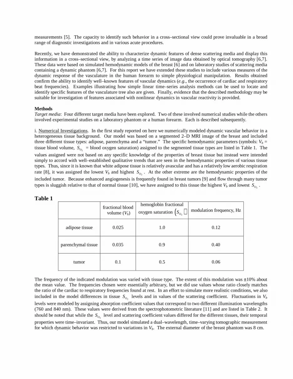
measurements [5]. The capacity to identify such behavior in a cross–sectional view could prove invaluable in a broad range of diagnostic investigations and in various acute procedures. Recently, we have demonstrated the ability to characterize dynamic features of dense scattering media and display this information in a cross–sectional view, by analyzing a time series of image data obtained by optical tomography [6,7]. These data were based on simulated hemodynamic models of the breast [6] and on laboratory studies of scattering media containing a dynamic phantom [6,7]. For this report we have extended these studies to include various measures of the dynamic response of the vasculature in the human forearm to simple physiological manipulation. Results obtained confirm the ability to identify well–known features of vascular dynamics (e.g., the occurrence of cardiac and respiratory beat frequencies). Examples illustrating how simple linear time–series analysis methods can be used to locate and identify specific features of the vasculature tree also are given. Finally, evidence that the described methodology may be suitable for investigation of features associated with nonlinear dynamics in vascular reactivity is provided. Methods Target media: Four different target media have been explored. Two of these involved numerical studies while the others involved experimental studies on a laboratory phantom or a human forearm. Each is described subsequently. i. Numerical Investigations. In the first study reported on here we numerically modeled dynamic vascular behavior in a heterogeneous tissue background. Our model was based on a segmented 2–D MRI image of the breast and included three different tissue types: adipose, parenchyma and a “tumor.” The specific hemodynamic parameters (symbols: Vb = tissue blood volume,

2OS = blood oxygen saturation) assigned to the segmented tissue types are listed in Table 1. The

values assigned were not based on any specific knowledge of the properties of breast tissue but instead were intended simply to accord with well–established qualitative trends that are seen in the hemodynamic properties of various tissue types. Thus, since it is known that white adipose tissue is relatively avascular and has a relatively low aerobic respiration rate [8], it was assigned the lowest Vb and highest

2OS . At the other extreme are the hemodynamic properties of the

included tumor. Because enhanced angiogenesis is frequently found in breast tumors [9] and flow through many tumor types is sluggish relative to that of normal tissue [10], we have assigned to this tissue the highest Vb and lowest

2OS .

Table 1

fractional blood

volume (Vb)

hemoglobin fractional

oxygen saturation ( )2OS modulation frequency, Hz

adipose tissue 0.025 1.0 0.12

parenchymal tissue 0.035 0.9 0.40

tumor 0.1 0.5 0.06

The frequency of the indicated modulation was varied with tissue type. The extent of this modulation was ±10% about the mean value. The frequencies chosen were essentially arbitrary, but we did use values whose ratio closely matches the ratio of the cardiac to respiratory frequencies found at rest. In an effort to simulate more realistic conditions, we also included in the model differences in tissue

2OS levels and in values of the scattering coefficient. Fluctuations in Vb

levels were modeled by assigning absorption coefficient values that correspond to two different illumination wavelengths (760 and 840 nm). These values were derived from the spectrophotometric literature [11] and are listed in Table 2. It should be noted that while the

2OS level and scattering coefficient values differed for the different tissues, their temporal

properties were time–invariant. Thus, our model simulated a dual–wavelength, time–varying tomographic measurement for which dynamic behavior was restricted to variations in Vb. The external diameter of the breast phantom was 8 cm.

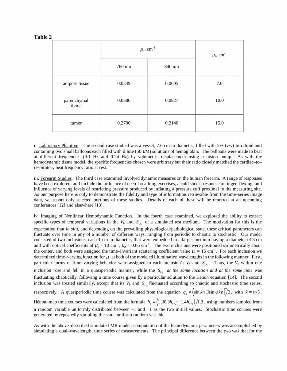
Table 2

Pa, cm-1

760 nm 840 nm

Ps, cm-1

adipose tissue 0.0349 0.0605 7.0

parenchymal tissue

0.0580 0.0827 10.0

tumor 0.2700 0.2140 15.0

ii. Laboratory Phantom. The second case studied was a vessel, 7.6 cm in diameter, filled with 2% (v/v) Intralipid and containing two small balloons each filled with dilute (50 µM) solutions of hemoglobin. The balloons were made to beat at different frequencies (0.1 Hz and 0.24 Hz) by volumetric displacement using a piston pump. As with the hemodynamic tissue model, the specific frequencies chosen were arbitrary but their ratio closely matched the cardiac–to–respiratory beat frequency ratio at rest. iii. Forearm Studies. The third case examined involved dynamic measures on the human forearm. A range of responses have been explored, and include the influence of deep–breathing exercises, a cold shock, response to finger–flexing, and influence of varying levels of restricting pressure produced by inflating a pressure cuff proximal to the measuring site. As our purpose here is only to demonstrate the fidelity and type of information retrievable from the time–series image data, we report only selected portions of these studies. Details of each of these will be reported at an upcoming conferences [12] and elsewhere [13]. iv. Imaging of Nonlinear Hemodynamic Function. In the fourth case examined, we explored the ability to extract specific types of temporal variations in the Vb and

2OS of a simulated test medium. The motivation for this is the

expectation that in situ, and depending on the prevailing physiological/pathological state, these critical parameters can fluctuate over time in any of a number of different ways, ranging from periodic to chaotic to stochastic. Our model consisted of two inclusions, each 1 cm in diameter, that were embedded in a larger medium having a diameter of 8 cm and with optical coefficients of µs = 10 cm-1, µa = 0.06 cm-1. The two inclusions were positioned symmetrically about the center, and both were assigned the time–invariant scattering coefficient value µs = 15 cm-1. For each inclusion we determined time–varying function for µa at both of the modeled illumination wavelengths in the following manner. First, particular forms of time–varying behavior were assigned to each inclusion’s Vb and

2OS . Thus, the Vb within one

inclusion rose and fell in a quasiperiodic manner, while the 2OS at the same location and at the same time was

fluctuating chaotically, following a time course given by a particular solution to the Hénon equation [14]. The second inclusion was treated similarly, except that its Vb and

2OS fluctuated according to chaotic and stochastic time series,

respectively. A quasiperiodic time course was calculated from the equation ( )sin sin 2,nq kn kn= + with 5k π= .

Hénon–map time courses were calculated from the formula ( )22 11 0.3 1.4 1.3,n n nh h h− −= + − using numbers sampled from

a random variable uniformly distributed between –1 and +1 as the two initial values. Stochastic time courses were generated by repeatedly sampling the same uniform random variable. As with the above–described simulated MR model, computation of the hemodynamic parameters was accomplished by simulating a dual–wavelength, time series of measurements. The principal difference between the two was that for the

present case, more complex time–series functions were assigned to Vb and 2OS , and the latter was made time–varying in

the present case while it had been constant in the previous one. The time series for Vb and 2OS were generated by

applying ( ) ( )0.05 1 0.2 ,b n nV t x= + ( ) ( )2O 0.7 1 0.2 ,n nS t y= + where xn and yn are any two of the preceding types of time

courses, thereby modeling 20% modulation about mean values of 5% Vb, 70% 2OS . [We are aware that in the case of the

Hénon map, the mean value is > zero when the extreme values are set equal to �1, as is the case here. Therefore, our chaotic Vb and

2OS time series actually have mean values somewhat greater than 5% and 70%, respectively. This

numerical detail is completely inconsequential for our purposes here.] According to the hemodynamic model described previously, the tissue absorption coefficients at the two measurement wavelengths must be

( ) ( ) ( ) ( )2Ored ox reda n b n a a a nt V t S tλ λ λλµ µ µ µ = + − ,

where the superscript O is the wavelength of the illumination, and oxaλµ and

oxaλµ are the absorption coefficients of

hemoglobin at the average concentrations that they have in whole blood, in the oxygenated and reduced (i.e., deoxygenated) states, respectively. Collection of Time–Series Detector Data: Tomographic data for the tissue model was acquired by using the finite element method to solve the diffusion equation with Dirichlet boundary conditions. The source/detector configuration used match those adopted in the experimental studies. In all cases, image formation was based on use of six source positions and eighteen detectors per source. Each source sequentially illuminated the target, while data were collected in parallel. Sources were positioned uniformly about the target at 60° intervals while detectors were positioned at 20° intervals. The sampling rate (simulated or real) varied depending on the experiment but in most cases was 2–4 Hz. In cases i–iii (as described above under Methods: Target Media), a total of 240–300 data points were collected for each time series, while for case iv the number was increased to 1000. Instrumentation: Time–series detector data from experimental studies were collected using a recently described optical imager [7]. The instrument functions as a serial–source, multi–channel, parallel–detection device. Figure 1 show a photograph of the iris imaging head used in these studies. By adjusting the pass–through diameter, optical fibers can be brought into gentle contact with the target medium. Depending on the study, measurements were performed at 2–4 Hz in either a single– (810 nm) or dual–wavelength (780 and 810 nm) mode.

Figure 1. Photograph of iris imaging head.

Preimage Analysis and Reconstruction: For each detector channel, optical data at each time point were normalized to a mean value of the recorded signal. For most studies, the mean value was computed from the data points corresponding to the initial 30 s of measurement. The normalized values were then used as the input data vectors for image recovery. Images were computed by simultaneously solving for the diffusion and absorption coefficients using a recently described

Rotating Cam

Probing Volume Bifurcated

Fiber Bundles

algorithm [15]. Computed solutions were limited to the first–order Born approximation using a CGD solver. Also, while both coefficients were computed, reported results here are restricted to estimates of the absorption coefficient. Computation of images revealing simulated hemodynamic function. To derive an image series revealing hemodynamic function required an additional post–processing step to merge information obtained at the two simulated measuring

wavelengths. Accordingly, estimates of Vb and 2OS were calculated from the reconstructed values of 760

tisaµ and 840

tisaµ in

each pixel and at each value of the time index, using the equations

( ) ( )840 840 760 760 760 840

red ox tis red ox tis

840 760 760 840

red ox red ox

,a a a a a a

b

a a a a

Vµ µ µ µ µ µ

µ µ µ µ

− − −=

− ( ) ( )2

840 760 760 840

red tis red tisO 840 840 760 760 760 840

red ox tis red ox tis

.a a a a

a a a a a a

Sµ µ µ µ

µ µ µ µ µ µ

−=

− − −

These equations were used to derive the hemodynamic time series for both the MR–derived model and for the simulated nonlinear studies. Image analysis. i. Linear time–series analysis. Where indicated, standard linear time–series analysis methods were employed to evaluate the image series [16]. For example, the frequency spectrum of the image time series was derived by computing the Fourier transform for each pixel. Other measures involved computing inter–pixel and detector–to–pixel cross–spectral density and coherence functions. ii. Nonlinear time–series analysis. Two forms of analysis were performed. The first involved computing the (pseudo–) state–space attractor using the method of delays [17]. The second measure involved computing a map of the correlation dimension for each using the method of Grassberger and Proccacia [18]. The correlation dimension Q is a measure of the complexity of the system being investigated. It is computed by analyzing the trajectory formed in an n–dimensional hyperspace plot. This trajectory fills a subspace of the state space and is called the system’s attractor. In general, the larger the value of Q, the more complicated is the behavior of the system under investigation; additionally, a non–integer value of Q is potentially diagnostic of chaotic dynamics. We are aware that the approaches adopted here to do not constitute a comprehensive characterization of the data, in particular with regard to the issue of distinguishing a truly nonlinear function from some other functional form. Other parameters have been computed (e.g., the effect of replacing an original data set with one or more surrogates [19]), but results of these studies will be reported elsewhere. Our purpose here is more demonstrational, so as to gain a sense of the distinguishability of different time–varying functions, and the accuracy with which they can be recovered. Results Enhanced Image Contrast of Dynamic Features. Improvement in image contrast and resolution is important for any imaging method. Thus far, optical imaging methods have produced only images having relatively low contrast and resolution from tissue studies. While refinements in data processing and instrument performance may improve this situation, at this point it would seem that these contrast and resolution levels might represent basic features of optical imaging. Recently we have shown [6,7] that images that identify dynamic behavior in the optical coefficients (e.g., amplitude of time–harmonic oscillations in µa) can produce spatial maps that have greatly improved quality compared to images of the spatial contrast in the optical coefficients per se. These can include amplitude and phase maps of the Fourier spectrum, and maps of temporal correlations and their frequency composition. As an example, in Figure 2 we show an original image of a complex target medium (a), a reconstructed map of its time–averaged Vb levels (b), and a map of the computed coherence at a selected frequency (c) computed from the same data shown in (b) and derived from analysis of a time series. The original is a 2–D coronal section of a MR mammogram, for which various optical properties (0.04 < µa < 0.3, 5 < µs < 15 cm-1) were assigned to the different tissue types [adipose (dark), parenchyma (gray) and tumor (light)] (see legend for description). Comparison shows the resolution and contrast of the time–averaged map is relatively low and the tumor is not evident. In contrast, the tumor is clearly revealed in the coherence image. Significantly, this result was obtained without any prior knowledge of the tumor’s presence, and instead is dependent solely on the tumor having a temporal response different from that of the surrounding tissue. Clinically, such behavior may exist naturally [20], or it could be induced in response to a simple manipulation of the vascular perfusion state. These findings thus demonstrate that high–

quality image data revealing the presence of dynamic behavior in a dense scattering medium can be derived from analysis of time series of images of a complex simulated phantom. Next we show results demonstrating that images of similar quality can be obtained from a laboratory phantom exhibiting dynamic behavior.

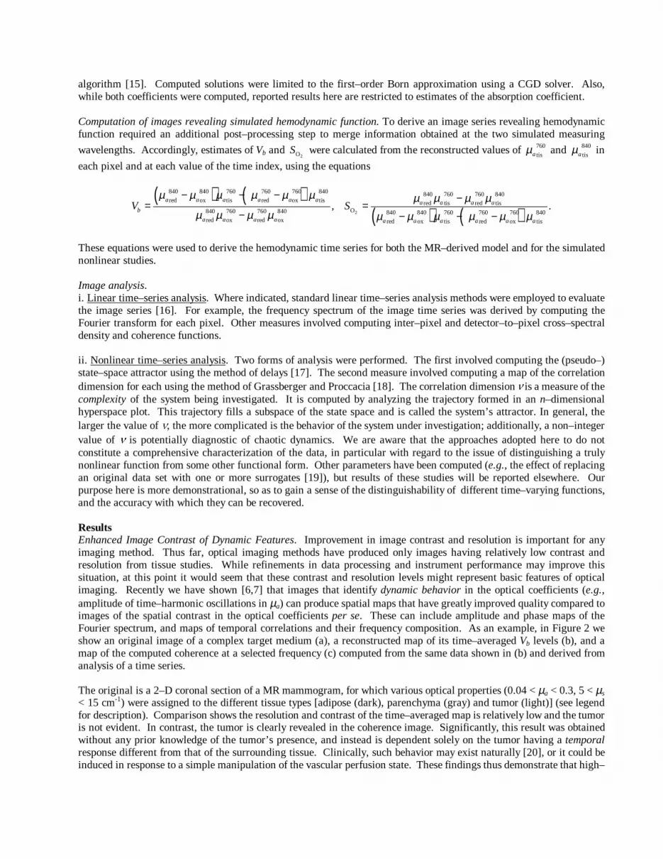
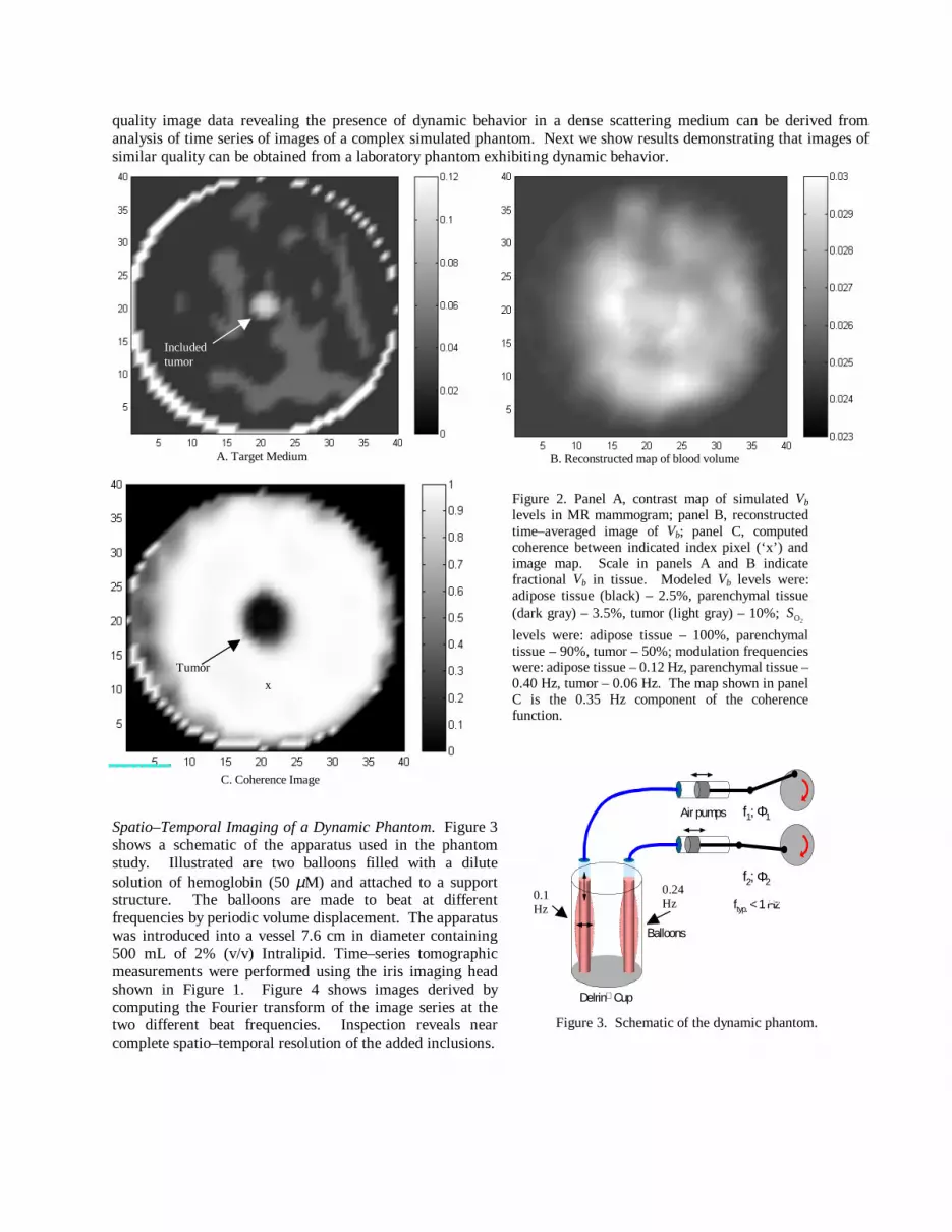
Spatio–Temporal Imaging of a Dynamic Phantom. Figure 3 shows a schematic of the apparatus used in the phantom study. Illustrated are two balloons filled with a dilute solution of hemoglobin (50 µM) and attached to a support structure. The balloons are made to beat at different frequencies by periodic volume displacement. The apparatus was introduced into a vessel 7.6 cm in diameter containing 500 mL of 2% (v/v) Intralipid. Time–series tomographic measurements were performed using the iris imaging head shown in Figure 1. Figure 4 shows images derived by computing the Fourier transform of the image series at the two different beat frequencies. Inspection reveals near complete spatio–temporal resolution of the added inclusions.

Figure 2. Panel A, contrast map of simulated Vb levels in MR mammogram; panel B, reconstructed time–averaged image of Vb; panel C, computed coherence between indicated index pixel (‘x’) and image map. Scale in panels A and B indicate fractional Vb in tissue. Modeled Vb levels were: adipose tissue (black) – 2.5%, parenchymal tissue (dark gray) – 3.5%, tumor (light gray) – 10%;

2OS

levels were: adipose tissue – 100%, parenchymal tissue – 90%, tumor – 50%; modulation frequencies were: adipose tissue – 0.12 Hz, parenchymal tissue – 0.40 Hz, tumor – 0.06 Hz. The map shown in panel C is the 0.35 Hz component of the coherence function.

Included tumor

C. Coherence Image

Tumor

x

B. Reconstructed map of blood volume A. Target Medium

f1; Φ1

f2; Φ2

ftyp. < 1 Hz

Balloons

Air pumps

Delrin Cup

0.24 Hz

0.1 Hz

0.1 Hz

Figure 3. Schematic of the dynamic phantom.

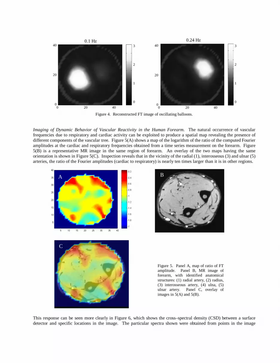
Figure 4. Reconstructed FT image of oscillating balloons. Imaging of Dynamic Behavior of Vascular Reactivity in the Human Forearm. The natural occurrence of vascular frequencies due to respiratory and cardiac activity can be exploited to produce a spatial map revealing the presence of different components of the vascular tree. Figure 5(A) shows a map of the logarithm of the ratio of the computed Fourier amplitudes at the cardiac and respiratory frequencies obtained from a time series measurement on the forearm. Figure 5(B) is a representative MR image in the same region of forearm. An overlay of the two maps having the same orientation is shown in Figure 5(C). Inspection reveals that in the vicinity of the radial (1), interosseous (3) and ulnar (5) arteries, the ratio of the Fourier amplitudes (cardiac to respiratory) is nearly ten times larger than it is in other regions.

This response can be seen more clearly in Figure 6, which shows the cross–spectral density (CSD) between a surface detector and specific locations in the image. The particular spectra shown were obtained from points in the image

3 2 1 0

40

20

0 0 20 40

40

20

0 0 20 40

3 2 1 0

0.1 Hz 0.24 Hz

Figure 5. Panel A, map of ratio of FT amplitude. Panel B, MR image of forearm, with identified anatomical structures: (1) radial artery, (2) radius, (3) interosseous artery, (4) ulna, (5) ulnar artery. Panel C, overlay of images in 5(A) and 5(B).

A B

C

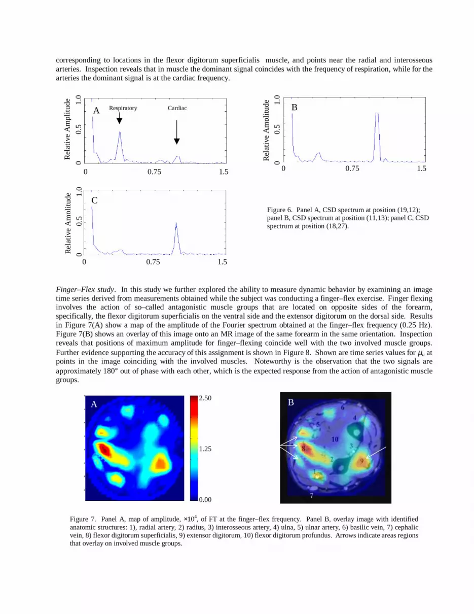
corresponding to locations in the flexor digitorum superficialis muscle, and points near the radial and interosseous arteries. Inspection reveals that in muscle the dominant signal coincides with the frequency of respiration, while for the arteries the dominant signal is at the cardiac frequency.

Finger–Flex study. In this study we further explored the ability to measure dynamic behavior by examining an image time series derived from measurements obtained while the subject was conducting a finger–flex exercise. Finger flexing involves the action of so–called antagonistic muscle groups that are located on opposite sides of the forearm, specifically, the flexor digitorum superficialis on the ventral side and the extensor digitorum on the dorsal side. Results in Figure 7(A) show a map of the amplitude of the Fourier spectrum obtained at the finger–flex frequency (0.25 Hz). Figure 7(B) shows an overlay of this image onto an MR image of the same forearm in the same orientation. Inspection reveals that positions of maximum amplitude for finger–flexing coincide well with the two involved muscle groups. Further evidence supporting the accuracy of this assignment is shown in Figure 8. Shown are time series values for µa at points in the image coinciding with the involved muscles. Noteworthy is the observation that the two signals are approximately 180° out of phase with each other, which is the expected response from the action of antagonistic muscle groups.

Figure 7. Panel A, map of amplitude, ×104, of FT at the finger–flex frequency. Panel B, overlay image with identified anatomic structures: 1), radial artery, 2) radius, 3) interosseous artery, 4) ulna, 5) ulnar artery, 6) basilic vein, 7) cephalic vein, 8) flexor digitorum superficialis, 9) extensor digitorum, 10) flexor digitorum profundus. Arrows indicate areas regions that overlay on involved muscle groups.

0 0.75 1.5

Rel

ativ

e A

mplit

ude

0

0.

5

1.0

0 0.75 1.5

Rel

ativ

e A

mplit

ude

0

0.

5

1.0

0 0.75 1.5

Rel

ativ

e A

mplit

ude

0

0.5

1.0

Respiratory Cardiac

Figure 6. Panel A, CSD spectrum at position (19,12); panel B, CSD spectrum at position (11,13); panel C, CSD spectrum at position (18,27).

A B

C

2.50 1.25 0.00

A B

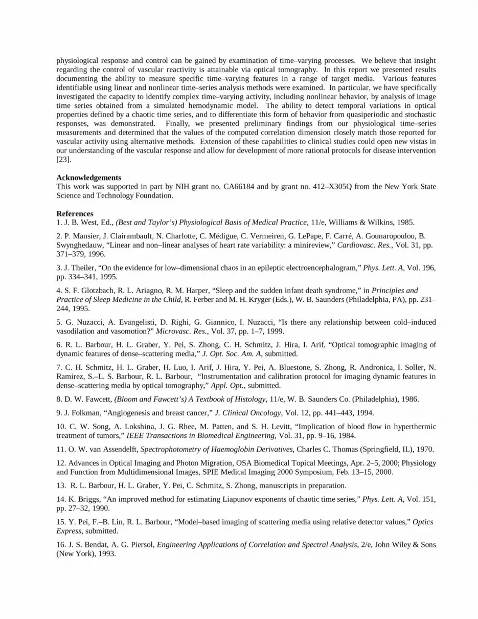
Figure 8. Time variations in µa for pixel locations in involved muscle groups. Imaging of Nonlinear Hemodynamic Function. Figure 9 shows the dependence of the computed pseudo–state–space attractor on the functional form of the time series introduced for the two measures of hemodynamic function. Recall, that in this study Vb and

2OS fluctuated in time according to different mathematical functions at the same time and

location. In each panel we also show the time function derived from the computed image series (upper left) at a designated index pixel shown by ‘x’ in the figure in the upper right. The latter is a representative image obtained from the time series. Results in Panel A show the attractor computed for a quasiperiodic time function in Vb for the left–hand–side inclusion. Panel C shows the corresponding results, at the same site, for variations in

2OS . Here a chaotic (Hénon

map) time series was introduced. Similarly, results in Panel B shows the attractor computed according to chaotic time series in Vb for the right–hand–side inclusion. Panel D shows the corresponding results, at the same site, for a stochastic time variability in

2OS . In each case inspection reveals markedly different forms of the attractor. These results further

demonstrate the remarkable accuracy with which the spatio–temporal features of vascular reactivity (simulated or real) can be recovered. Figure 9

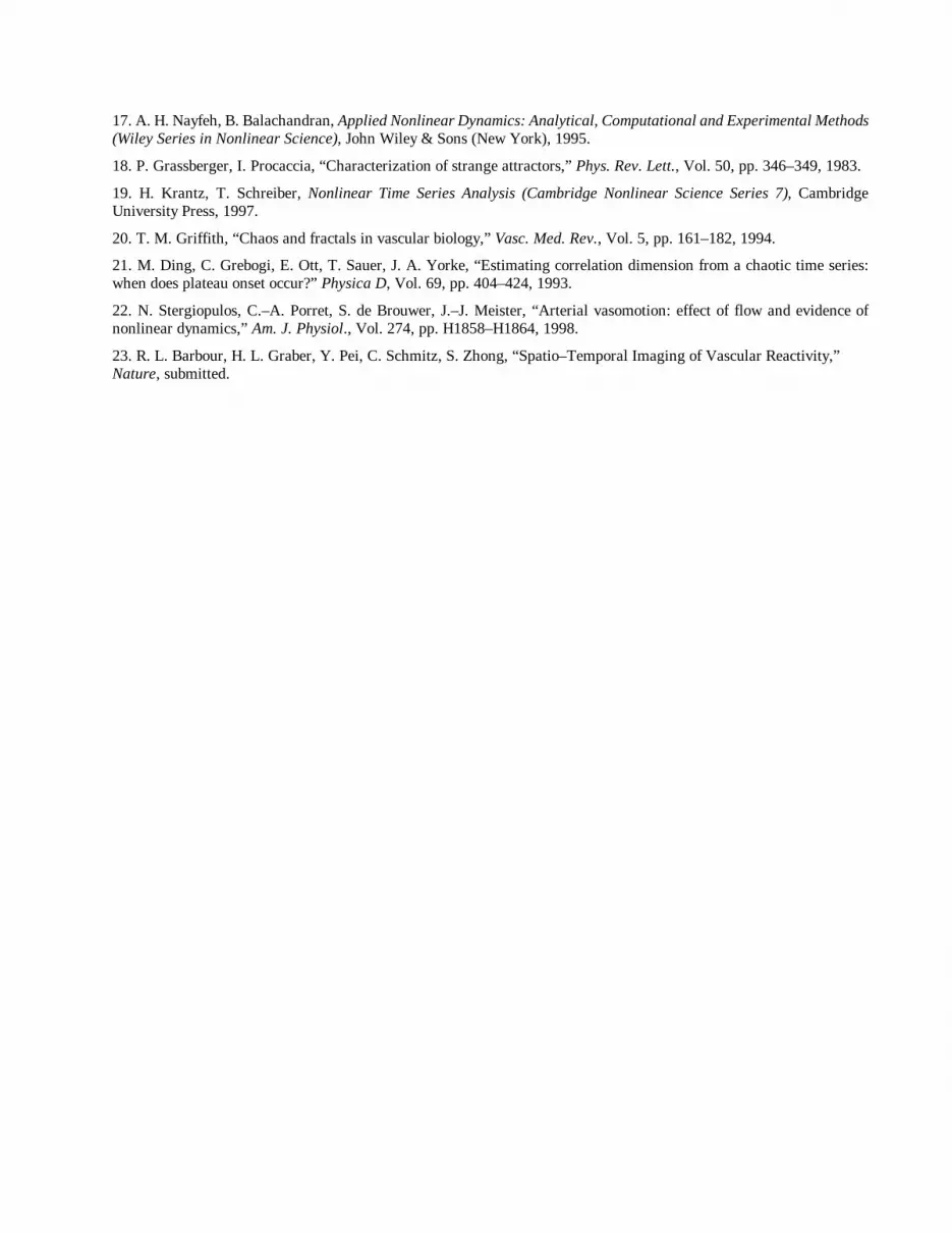
Finally, in Figure 10 we show results obtained from a physiological time series (a series of deep breathing exercises) for which we computed a spatial map of the correlation dimension at each pixel location. Recall that the correlation dimension is a measure of the complexity of a time series. Here we selected a frequency passband that included both the vasomotor and respiratory frequencies (0.05–0.5 Hz). We are aware that such filtering colors the noise and can lead to spurious low correlation dimension values [21]. For this reason we also treated data obtained from a stochastic time

0 7.5 15 Time (sec)

Row 14, column 31

2 4 6 8 0 2 4 6

0

0

0 row 19 Column 9 Row 19, column 9

0

0

.5

1.0

Rel

ativ

e A

mpl

itude

0 7.5 15 Time (sec)

A

B

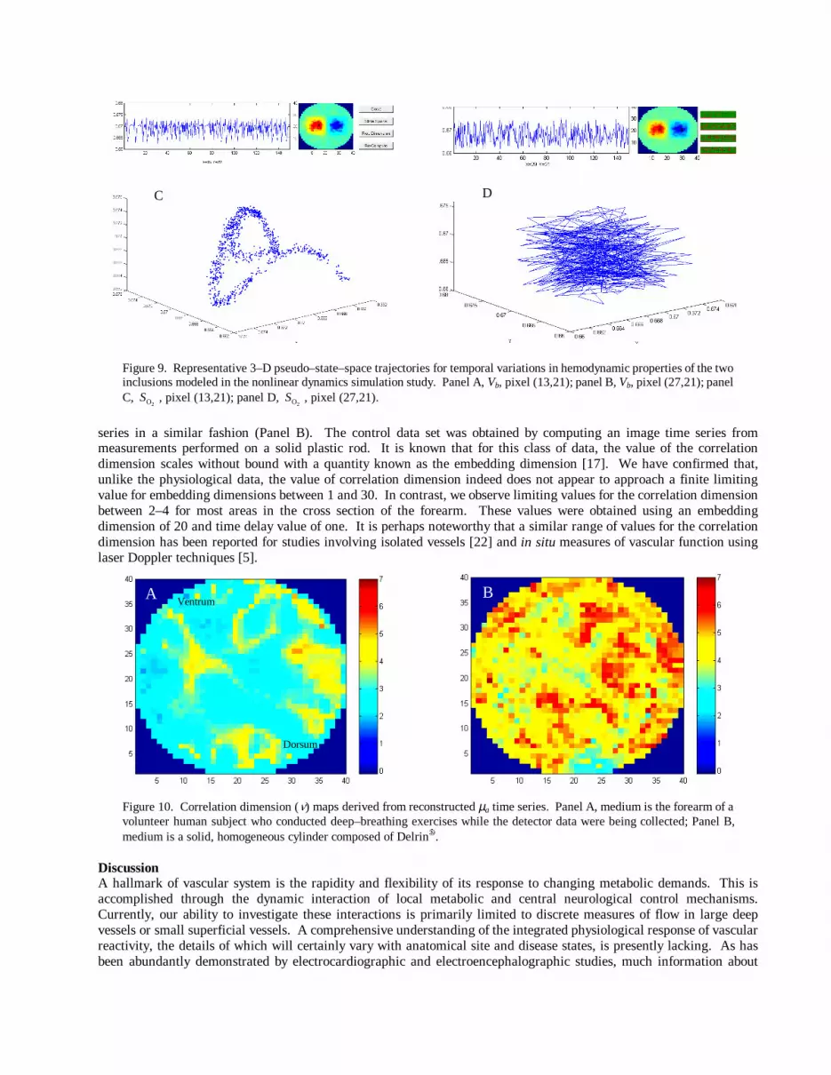
Figure 9. Representative 3–D pseudo–state–space trajectories for temporal variations in hemodynamic properties of the two inclusions modeled in the nonlinear dynamics simulation study. Panel A, Vb, pixel (13,21); panel B, Vb, pixel (27,21); panel C,

2OS , pixel (13,21); panel D, 2OS , pixel (27,21).

series in a similar fashion (Panel B). The control data set was obtained by computing an image time series from measurements performed on a solid plastic rod. It is known that for this class of data, the value of the correlation dimension scales without bound with a quantity known as the embedding dimension [17]. We have confirmed that, unlike the physiological data, the value of correlation dimension indeed does not appear to approach a finite limiting value for embedding dimensions between 1 and 30. In contrast, we observe limiting values for the correlation dimension between 2–4 for most areas in the cross section of the forearm. These values were obtained using an embedding dimension of 20 and time delay value of one. It is perhaps noteworthy that a similar range of values for the correlation dimension has been reported for studies involving isolated vessels [22] and in situ measures of vascular function using laser Doppler techniques [5].

Figure 10. Correlation dimension (Q) maps derived from reconstructed µa time series. Panel A, medium is the forearm of a volunteer human subject who conducted deep–breathing exercises while the detector data were being collected; Panel B, medium is a solid, homogeneous cylinder composed of Delrin´.

Discussion A hallmark of vascular system is the rapidity and flexibility of its response to changing metabolic demands. This is accomplished through the dynamic interaction of local metabolic and central neurological control mechanisms. Currently, our ability to investigate these interactions is primarily limited to discrete measures of flow in large deep vessels or small superficial vessels. A comprehensive understanding of the integrated physiological response of vascular reactivity, the details of which will certainly vary with anatomical site and disease states, is presently lacking. As has been abundantly demonstrated by electrocardiographic and electroencephalographic studies, much information about

D

Ventrum

Dorsum

A B

C

physiological response and control can be gained by examination of time–varying processes. We believe that insight regarding the control of vascular reactivity is attainable via optical tomography. In this report we presented results documenting the ability to measure specific time–varying features in a range of target media. Various features identifiable using linear and nonlinear time–series analysis methods were examined. In particular, we have specifically investigated the capacity to identify complex time–varying activity, including nonlinear behavior, by analysis of image time series obtained from a simulated hemodynamic model. The ability to detect temporal variations in optical properties defined by a chaotic time series, and to differentiate this form of behavior from quasiperiodic and stochastic responses, was demonstrated. Finally, we presented preliminary findings from our physiological time–series measurements and determined that the values of the computed correlation dimension closely match those reported for vascular activity using alternative methods. Extension of these capabilities to clinical studies could open new vistas in our understanding of the vascular response and allow for development of more rational protocols for disease intervention [23]. Acknowledgements This work was supported in part by NIH grant no. CA66184 and by grant no. 412–X305Q from the New York State Science and Technology Foundation. References 1. J. B. West, Ed., (Best and Taylor’s) Physiological Basis of Medical Practice, 11/e, Williams & Wilkins, 1985.

2. P. Mansier, J. Clairambault, N. Charlotte, C. Médigue, C. Vermeiren, G. LePape, F. Carré, A. Gounaropoulou, B. Swynghedauw, “Linear and non–linear analyses of heart rate variability: a minireview,” Cardiovasc. Res., Vol. 31, pp. 371–379, 1996.

3. J. Theiler, “On the evidence for low–dimensional chaos in an epileptic electroencephalogram,” Phys. Lett. A, Vol. 196, pp. 334–341, 1995.

4. S. F. Glotzbach, R. L. Ariagno, R. M. Harper, “Sleep and the sudden infant death syndrome,” in Principles and Practice of Sleep Medicine in the Child, R. Ferber and M. H. Kryger (Eds.), W. B. Saunders (Philadelphia, PA), pp. 231–244, 1995.

5. G. Nuzacci, A. Evangelisti, D. Righi, G. Giannico, I. Nuzacci, “Is there any relationship between cold–induced vasodilation and vasomotion?” Microvasc. Res., Vol. 37, pp. 1–7, 1999.

6. R. L. Barbour, H. L. Graber, Y. Pei, S. Zhong, C. H. Schmitz, J. Hira, I. Arif, “Optical tomographic imaging of dynamic features of dense–scattering media,” J. Opt. Soc. Am. A, submitted.

7. C. H. Schmitz, H. L. Graber, H. Luo, I. Arif, J. Hira, Y. Pei, A. Bluestone, S. Zhong, R. Andronica, I. Soller, N. Ramirez, S.–L. S. Barbour, R. L. Barbour, “Instrumentation and calibration protocol for imaging dynamic features in dense–scattering media by optical tomography,” Appl. Opt., submitted.

8. D. W. Fawcett, (Bloom and Fawcett’s) A Textbook of Histology, 11/e, W. B. Saunders Co. (Philadelphia), 1986.

9. J. Folkman, “Angiogenesis and breast cancer,” J. Clinical Oncology, Vol. 12, pp. 441–443, 1994.

10. C. W. Song, A. Lokshina, J. G. Rhee, M. Patten, and S. H. Levitt, “Implication of blood flow in hyperthermic treatment of tumors,” IEEE Transactions in Biomedical Engineering, Vol. 31, pp. 9–16, 1984.

11. O. W. van Assendelft, Spectrophotometry of Haemoglobin Derivatives, Charles C. Thomas (Springfield, IL), 1970.

12. Advances in Optical Imaging and Photon Migration, OSA Biomedical Topical Meetings, Apr. 2–5, 2000; Physiology and Function from Multidimensional Images, SPIE Medical Imaging 2000 Symposium, Feb. 13–15, 2000.

13. R. L. Barbour, H. L. Graber, Y. Pei, C. Schmitz, S. Zhong, manuscripts in preparation.

14. K. Briggs, “An improved method for estimating Liapunov exponents of chaotic time series,” Phys. Lett. A, Vol. 151, pp. 27–32, 1990.

15. Y. Pei, F.–B. Lin, R. L. Barbour, “Model–based imaging of scattering media using relative detector values,” Optics Express, submitted.

16. J. S. Bendat, A. G. Piersol, Engineering Applications of Correlation and Spectral Analysis, 2/e, John Wiley & Sons (New York), 1993.

17. A. H. Nayfeh, B. Balachandran, Applied Nonlinear Dynamics: Analytical, Computational and Experimental Methods (Wiley Series in Nonlinear Science), John Wiley & Sons (New York), 1995.

18. P. Grassberger, I. Procaccia, “Characterization of strange attractors,” Phys. Rev. Lett., Vol. 50, pp. 346–349, 1983.

19. H. Krantz, T. Schreiber, Nonlinear Time Series Analysis (Cambridge Nonlinear Science Series 7), Cambridge University Press, 1997.

20. T. M. Griffith, “Chaos and fractals in vascular biology,” Vasc. Med. Rev., Vol. 5, pp. 161–182, 1994.

21. M. Ding, C. Grebogi, E. Ott, T. Sauer, J. A. Yorke, “Estimating correlation dimension from a chaotic time series: when does plateau onset occur?” Physica D, Vol. 69, pp. 404–424, 1993.

22. N. Stergiopulos, C.–A. Porret, S. de Brouwer, J.–J. Meister, “Arterial vasomotion: effect of flow and evidence of nonlinear dynamics,” Am. J. Physiol., Vol. 274, pp. H1858–H1864, 1998.

23. R. L. Barbour, H. L. Graber, Y. Pei, C. Schmitz, S. Zhong, “Spatio–Temporal Imaging of Vascular Reactivity,” Nature, submitted.