TWO STATISTICAL PROBLEMS IN THE PRINCETON PROJECT …aida.wss.yale.edu/growth_pdf/cdp869.pdf · The Princeton Project on the Decline of Fertility in Europe (or European Fertility

ECONOMIC GROWTH CENTER

YALE UNIVERSITY

P.O. Box 208269New Haven, CT 06520-8269

http://www.econ.yale.edu/~egcenter/

CENTER DISCUSSION PAPER NO. 869

TWO STATISTICAL PROBLEMS IN THE PRINCETON PROJECT ONTHE EUROPEAN FERTILITY TRANSITION

John C. BrownClark University

and

Timothy W. GuinnaneYale University

September 2003

Notes: Center Discussion Papers are preliminary materials circulated to stimulate discussions and criticalcomments.

An earlier version of this paper was circulated under a slightly different title, and was revised whileGuinnane was visiting the Faculty of Economics at the University of Cambridge. The paper is partof a larger project; see Brown, Guinnane, and Lupprian (1993) and Brown and Guinnane (2002) foradditional discussion. For comments and suggestions we are grateful to Jan van Bavel, TheoEngelen, Avery Guest, Sriya Iyer, Christopher Meissner, Carolyn Moehling, Mary MacKinnon,Sheilagh Ogilvie, Cormac Ó Gráda, Barbara Okun, Matthias Schuendeln, and seminar participantsat the Cambridge Group for the History of Population and Social Structure and the N.W. PosthumusInstitute. This research was supported by the National Institute of Child Health and HumanDevelopment. We are especially grateful to Patrick Galloway for his comments and for helping usto construct extracts from his Prussian data.

This paper can be downloaded without charge from the Social Science Research Network electroniclibrary at: http://ssrn.com/abstract=445901

An index to papers in the Economic Growth Center Discussion Paper Series is located at: http://www.econ.yale.edu/~egcenter/research.htm

Two Statistical Problems in the Princeton Project

On the European Fertility Transition

John C. BrownDepartment of Economics, Clark University

Worcester, MA [email protected]

Timothy W. GuinnaneDepartment of Economics, Yale University

New Haven, CT [email protected]

Abstract

The Princeton Project on the Decline of Fertility in Europe (or European Fertility Project, hereafterEFP) was carried out at Princeton University’s Office of Population Research in the 1960s and 1970s. This project aimed to characterize the decline of fertility that took place in Europe during the nineteenthand early twentieth centuries. The project’s summary statements argued that social and economicforces played little role in bringing about the fertility transition. The statement stresses instead a processof innovation and diffusion. A central feature of the EFP argument is a series of statistical exercises thatpurport to show that changes in economic and social conditions exerted little influence on fertility. Tworecent papers on Germany for this period have used similar data and methods to draw differentconclusions. These findings echo those of researchers working in other contexts, who increasingly findthat economic and social factors play a strong role in fertility. We show that one reason for the newfindings is some general statistical problems in the Princeton methodology. These are reason to temperacceptance of the Princeton project’s larger message.

Keyword: fertility transition

JEL codes: J13, N33, O15

The Princeton Project on the Decline of Fertility in Europe was alarge-scale research project undertaken by the late Ansley Coale and his col-laborators at Princeton’s Office of Population Research in the 1960s and1970s. The project compiled measures defined at the level of administrativeareas for most western European countries and used this data to study thepatterns of fertility decline and its correlation with possible explanatory fac-tors. This research has been extremely influential,because of the project’sscope and the skill and ingenuity of the individual studies. The project’soverall conclusion, often called the “Princeton view,” downplayed the im-portance of economic and social change in causing the fertility transition inEurope, and instead stressed a process of innovation and diffusion, driven bysimilar attitudes and communication networks.Two recent studies of Germany in the late nineteenth and early twenti-

eth centuries come to quite different conclusions. Patrick Galloway, EugeneHammel, and Ronald Lee (hereafter GHL) studied Prussia, the largest of theGerman states, while our own research (hereafter BG) focused on Bavaria,which was the next-largest state. Both projects find a clear role for theeconomic and social forces that the Princeton project (hereafter “EFP” )downplayed. These new results for Germany build on a much earlier paperby Toni Richards, who used the data underlying John Knodel’s EFP mono-graph on Germany to come to conclusions at variance with his own. Thedifference in results is surprising because both of the more recent studiesbear strong similarities to the EFP approach, while Richards’ study is baseddirectly on the EFP data.This paper argues that much of the difference can be attributed to two

problems in the statistical methods used by the Princeton authors. Theseproblems are quite general and would affect studies other than those for Ger-many.1 Our argument suggests caution in accepting the EFP conclusions.But our critique should not be exaggerated; we cannot show that the otherEFP studies were wrong, we can only demonstrate the problems in the Ger-man case and note that related problems might affect other studies. On asimilar note, we want to stress at the outset that the weaknesses we identifyhere reflect in a real way the EFP’s strengths. The first problem we dis-

1 Galloway et al (1998b, pp.195-208) surveys the methods used in recent research onthe fertility transition. A recent paper by Potter et al (2002) uses methods similar tothose advocated here, and also comes to the conclusion that social and economic forceshave not been given due weight in explaining the fertility transition. The context for thatpaper is modern Brazil.

3

cuss is a natural consequence of the EFP’s scope, and the second reflects itspioneering status.We focus on two distinct issues.

• The use of aggregate data necessarily leads to a loss of efficiency inestimation. The GHL and BG studies both use aggregate data, butthe administrative areas used in these studies are much smaller thanthose in the EFP, reducing the problem considerably.

• Coale’s vision of the fertility transition focused very much on changeover time. He argued that cross-area, pre-transition fertility levelsmight be interesting in their own right, but that these levels were notinformative about the transition itself. Much of the statistical analysisactually undertaken by the EFP authors was, however, cross-sectional.Some of its analysis that was not cross-sectional still does not dealwith important issues that arise in analysis of change over time. As wedemonstrate, some of the differences between the Richards, GHL, andBG studies on the one hand, and the original Knodel monograph onGermany on the other, reflect the use of statistical models that moreaccurately differentiate cross-sectional from time-series changes.

The paper is not intended as an omnibus discussion of the Europeanfertility transition or even the methods of the Princeton project. We focuson our two points and the interpretative issues they raise, and leave to otherworks (including our own) larger issues of interpretation and explanation.

1 The EFP and its vision

The project, it should be noted, was not originally conceived to address thequestions we raise here. Coale and his collaborators originally designed theEFP to test the validity of the classical demographic transition theory in theEuropean historical context. Coale noted as early as 1967 that the EFP datadid not support transition theory, and a conference held in 1968 focused onwhat appeared to be the futility of any unified theory of the fertility transi-tion. Subsequent work by the EFP scholars moved increasingly towards theregional and cultural arguments found in the summary statements.2 Thus

2 For discussion of the EFP’s history, see Friedlander, Okun, and Segal (1999, pp.497-500). This exceptionally clear and comprehensive review warrants reading by anyone

4

the project’s original conception, which is to say its original goals and theintellectual atmosphere in which it was initiated, played a strong role in cre-ating the problems we identify here. The large administrative areas usedin the project were probably sufficient to determine the inadequacy of theclassic demographic transition model, as Coale argued. Only from the van-tage of hindsight can one see, as we argue, that the statistical tools usedby the project were not consistent with Coale’s ultimate view of the fertilitytransition.The EFP studies all took a slightly different approach to their country,

reflecting data availability and the judgments of the individual author. Wewill not discuss any single work in detail, and by focusing on the statisticalwork we are overlooking thoughtful discussions of the fertility transition.In our characterization of the statistical methods used in the EFP we arethinking primarily of three monographs because these three contain the mostextensive statistical analysis: Germany [Knodel (1974)], Belgium [Lesthaeghe(1977)], and Italy [Livi-Bacci (1977)].3 Each of these studies shaped itself tothe available information, the interests and concerns of the author, and thespecifics of the country under study. There was a common EFP methodologyin the following sense:

Units of analysis: All Princeton studies were based on aggregate datadefined over administrative areas. The primary effort of the project wasto compute a common series of fertility indices for each of these provinces,starting before the fertility transition. The EFP studies then examined thepace of change in the several provinces.

Measuring rods: The EFP authors relied on a set of four inter-relatedindices that in effect compare fertility in the population under study tothe fertility of the Hutterites, a North American Anabaptist sect with well-documented, very high fertility. These indices were devised specially for usewith the project. The index of marital fertility (Ig) can be thought of as theratio of legitimate births in the population to the number of births one wouldexpect in a Hutterite population with the same number of married womenof the same ages. The index of proportions married (Im) weights the pro-

interested in these issues.3 The Office of Population Research’s website (www.opr.princeton.edu) has a list of all

publications associated with the project. Our bibliography lists those most relevant to ourdiscussion.

5

portions married at each age by the age-specific Hutterite fertility schedules.The index of non-marital fertility (Ih) is defined analogously to (Ig).4 Overallfertility (If) is thus defined as the weighted sum of marital and non-maritalfertility, where the weights are the index of proportions married:

If = Im ∗ Ig + (1− Im) ∗ Ih (1)

Measures of social and economic change: Most EFP studies use publishedinformation defined over the administrative areas to study the correlationbetween change in fertility on the one hand and social and economic de-velopment on the other. These measures include measures of urbanization,literacy, religion, and workforce allocation between agricultural and otherpursuits, and other variables.

Statistical methods: All of the monographs estimate correlation or re-gression models intended to ask whether some variables or combination ofvariables can explain the patterns of fertility decline.

None of the monographs confined themselves to this methodology alone.All of them introduce other information and follow-up on issues suggested bythe subject-matter or the author’s own interests, and several of them makesubtle use of data that did not fit into the common EFP methodology.

1.1 Conceptions of the fertility transition

Many discussions of the EFP turn on stated or unstated disagreements aboutwhat the fertility transition was, rather than what caused it. We have somereservations about the EFP image of a fertility transition. But to maintainour focus in this paper we set them aside in favor of asking how well the var-ious studies applied Coale’s notion to the concrete historical circumstance.Coale (1986) describes the major elements. Prior to the fertility transitionall populations were characterized by natural fertility, Coale argued, so thefertility transition is the point at which some significant part of the popula-tion has adopted fertility-control measures. Coale, like Louis Henry beforehim, defined natural fertility as the absence of parity-specific fertility con-trol. Parity-specific control means that the probability that a woman has her

4 The indices lie between 0 and 1, but many authors find it convenient to multiplythem by 1000. Appendix A provides definitions.

6

N + 1st birth t months after the last birth depends on N . Natural fertilityis consistent with a wide array of completed families sizes or fertility levels.The EFP found that most provinces in Europe experienced a plateau in

the level of marital fertility for some years prior to the transition. The levelof this plateau varied widely; the mean of Ig was about .72, but ranged from.5 to nearly 1. Why did the level of marital fertility vary so much, evenin populations that were (by assumption) not controlling fertility? As Coaleexplained it, “Marital fertility varied from one population to another becauseof differences in the prevalence and average duration of breast-feeding, peri-odic separation of spouses, etc.” (Coale 1986, p.35). Coale argued that suchvariations are consistent with natural fertility.These variations are not inconsistent with natural fertility. Rather, vari-

ations in the level of natural fertility were driven by local differences in be-haviors that affected fertility but that did not, in Coale’s vision, constituteconscious fertility control. The fertility transition itself is simpler:

In the typical history of marital fertility in Europe, the plateauof Ig was interrupted by a decline that began at the time of theinitiation of contraception or abortion (or both) among a largeenough segment of the population to affect aggregate marital fer-tility; Ig then continued to fall, reaching a minimum in almost allinstances ... of at least 50 percent below the plateau. An impor-tant feature of the history of Ig within each province is the dateat which the sustained decline began. The decline is character-ized as sustained because it was generally monotonic, except forpostwar reversals, and continued to fall until a greatly reducedlevel was reached (Coale 1986, p.37).

Coale suggested that a convenient operational definition of the fertilitytransition was the date at which Ig had first fallen by 10 percent. This cut-off was selected on the grounds that once marital fertility declined this muchit never rose again, so a 10-percent decline was safely irreversible. SeveralEFP monographs experiment with different (operational) definitions of thetransition, but most focus on a ten-percent decline in Ig.Coale’s vision of the fertility transition, then, is that different administra-

tive areas had very different pre-transition levels of natural fertility, depend-ing on breast-feeding, spousal separation, etc. But he focused on changes infertility.

7

1.2 Findings and interpretations

The EFP view on the relative unimportance of social and economic change isbest understood within the context of a distinction laid out in a paper thatwas not part of the project itself. Carlsson (1966)’s two alternatives motivatemany studies of the fertility transition. He put explanations of the fertilitytransition into one of two categories – innovation/diffusion or adaptation.5

The innovation/diffusion view claims that the adoption of fertility controlwithin a population represents a new behavior. The underlying reasons forthe new behavior could be new medical knowledge, or new ways of commu-nicating old knowledge, or changes in notions about the role of women infamilies or the moral acceptability of contraception. The adaptation view,on the other hand, claims that fertility control reflects couples’ adaptation tochanging economic and social circumstances. This distinction may not be asuseful today as it was when Carlsson published his paper, but it is importantto understanding the framework used by the Princeton studies.The approach taken in the EFP monographs, and the broader interpreta-

tion advanced in the summary statements, are consistent with the followingoperational approach, which is a basic strategy in all empirical social sci-ence.6 The project uses as its null hypothesis “changes in an indicator or setof indicators that proxy for social and economic change cannot explain thechange in fertility.” The alternative is “they can.” The point of the empiricalwork is to construct statistical tests of the null; we see if the data can rejectthe null hypothesis that changes in some X have no effect on fertility. TheEFP summary statements say that the studies could not reject the null.This view that the proxies for social and economic change do not explain

variations in the fertility transition is sometimes stated directly. A more com-mon way to state the EFP conclusions is to say that the fertility transitionoccurred at virtually the same time across the provinces of Europe. Coale(1986) notes that for Europe as a whole, 53 percent of all administrative areasexperienced their fertility transition between 1890 and 1920. For an event tohave a common cause across European societies, the logic goes, there must

5 Bean et al (1991) is an important study by historical demographers who stress theadaptation hypothesis. We are following their use of the term “adaptation” rather thanCarlsson’s term, “adjustment.”

6One can ask serious questions about what the two different types of fertility transitionwould look like in practice, and what kind of data one would need to distinguish the two.But devising perfect tests is not our aim here. What is important is the relationshipbetween the ideas and the empirical work.

8

be common features of those societies at the time of the fertility transition.But the project says there was not, or at least not enough to account forthis apparent simultaneity in transitions. Knodel and van de Walle (1986)draw this inference from the information they summarize in their Table 10.1.This kind of observation is probably the source of the scholarly shorthandthat says the EFP concluded that the only variable that explains the fertilitytransition is “date.” In their more general criticism of “demand theories” ofthe fertility transition, Cleland and Wilson make a similar point: “clearly thesimultaneity and speed of the European transition makes it highly doubtfulthat any economic force could be found which was powerful enough to offera reasonable explanation” (Cleland and Wilson 1987, p. 18).The EFP and its individual authors brought to bear a common set of

techniques and evidence, along with many original contributions. But thestatistical work about which we have reservations was central to the rejec-tion of the adaptation view of the transition. As one of the more influentialparticipants in the project put it, “Given the rough coincidence of modern-ization and the demographic transition, and the persuasiveness of the storiesthat were told to explain their relation, it is surprising that in country af-ter country, the tests of the hypotheses embedded in demographic transitiontheory produced no certain confirmation of the theory” (Watkins, 1986, pp.436-437). The repeated finding of the same, negative result for country aftercountry played an important role in convincing the EFP participants, andothers, of the validity of their view.Are these conclusions warranted? In our view they must be tempered by

an appreciation of the methodological problems we describe here. Our twopoints suggest that the EFP studies all reached similar conclusions in partbecause they all used methods that suffer from serious flaws. To provide con-creteness we will use two historical data sets and some very simple statisticalmodels in an effort to replicate the main tools of the Princeton project. Ifwe could, we would estimate what we think are the right statistical modelsusing the EFP data, and compare our new results to what was reported inthe monographs. This is unfortunately not possible, for two different reasons.To address our first point we would need completely different datasets thanthose assembled by the Princeton project. We only have the “right” data forPrussia and Bavaria, that is, from the GHL and BG projects. Addressingour second point would be possible if the Princeton project had made all itsdata publicly available, but it did not.The data are unavailable not becausethe project researchers are uncooperative, but because the various studies

9

were handled individually and at a time that predates widespread sharingof data in this form. With one exception, the project has made availablethe fertility indices but not the right-hand side variables required to estimatethe explanatory models.7 The exception is Germany, and for that exceptionthe models we think are correct have been estimated and published by ToniRichards. We discuss her paper below.

1.3 Illustrative examples

Our datasets are from the German kingdoms of Prussia (1875-1910) andBavaria (1880-1910). Galloway, Hammel and Lee have used the Prussiandata in their published work, while we have used the Bavarian data for asubstantive paper and use it here to provide concrete examples.8 Both Ger-man datasets are based on units of observation that are much smaller thanin Knodel’s study. His data set is based on published information from 71administrative areas in Germany, 30 of which are in Prussia. The Prussiandataset is based on the Kreis, the smallest administrative unit for which mostdata is available. The GHL team created 407 constant-territory Kreise, withobservations every 5 years for the period 1875-1910. Bavaria in the latenineteenth century had eight provinces, and in Knodel’s dataset Bavariacontributed eight observations. Our dataset is based on the Bezirksamt, thesmallest administrative unit in the seven Bavarian provinces right of theRhine.9 We focus on the 138 rural districts, for which we have observationson 1880, 1885, 1895, 1900, and 1910. A full description of the source andmore detailed variable definitions can be found in the published papers. Forconvenience we will refer to the small units (whether Kreise or Bezirksämter)as “districts.” In both Prussia and Bavaria the larger unit that correspondsto Knodel’s unit of analysis was called a Regierungsbezirk, which we will calla “province.” We have and will continue to use the term “administrativearea” in a neutral sense.The differences in degrees of aggregation here are very large. In Knodel’s

dataset, the average Prussian province has a population of more than 900

7 All available data have been posted at: http://opr.princeton.edu/archive/eufert.8The Prussia data were kindly provided by Patrick Galloway. An earlier version of

this paper also used simulated datasets. The results of those exercises are available uponrequest.

9 Bavaria had an eighth province, the Palatinate, whose districts are not comparableto those in the rest of Bavaria. Descriptive statistics can be found in Appendix B.

10

thousand. In the GHL data the average district in 1900 has a population ofabout one-twelfth that figure. In the BG data the average Bavarian districtis one-twentieth the size of the counterpart provinces in the Knodel dataset.Our examples take a simple form: we regress the general marital fertility

rate (GMFR) on the proportion of the district that is Catholic and the pro-portion that is urban.10 This serves as a sort of “ideal type” of regressionfrom this literature. Catholicism was expected to have a positive impact onfertility levels, and a negative impact on its decline, and in our examplescan be thought of as the “cultural” or “ideational” variable. Urbanization’sexpected impact is just the opposite, and can be viewed here as the “so-cial structure” or “economic” variable. No participant in debates about thefertility transition will find this an adequate model. There are many othervariables to consider, and both the GHL and BG papers demonstrate the im-portance of richer economic information. But this simple model works nicelyto illustrate the purely statistical points at issue here. The problems we il-lustrate here would affec both a richer model and a very simple model withdifferent right-hand side variables. The model we use has the great virtue ofhaving variables with the same definitions in Prussia and in Bavaria.11

2 The effects of aggregation

The EFP was based, perforce, on analysis of aggregate data. The project’sscope made use of individual-level data impractical. There are some draw-backs to ecological analysis that cannot be surmounted with any type of ag-gregate data, but when aggregate data are all that is available (or, in the caseof the Princeton project, all that is really compatible with the project’s aims)

10 The GMFR is defined as the number of legitimate births per married woman aged15-49. Some of the EFP studies use the framework of partial correlation instead of linearregression. The two approaches are very similar, and what we say here would also applyto models of partial correlation.11There is one difference. The Prussian districts comprise all of Prussia. Some districts,

in fact, are 100 percent urban (such as the city-Kreis of Berlin). The Bavarian districts,on the other hand, are the rural administrative units of the kingdom. “Rural” for Bavariameant “not having the legal status of a city” and in some cases our Bavarian districtsare quite urban. This would be a serious problem if our aim were to make historicalstatements about Prussia and Bavaria, but that has been done already elsewhere. In allthe examples given below, dropping the most urban Prussian districts did not materiallyaffect the results.

11

those drawbacks must be accepted as the price of scope. The monograph au-thors were all aware of one statistical problem implicit in using aggregatedata. Suppose we regress Ig on the proportion Catholic and the propor-tion urban. The estimates would tell us nothing about whether Catholiccity-dwellers have higher or lower fertility than Protestant city-dwellers. Wecannot claim that the regression coefficients from the aggregate data canrecover individual effects. Claiming otherwise is to commit the “ecologicalfallacy,” which none of the Princeton studies do.12

There is a different, serious problem caused by the large size and inter-nal heterogeneity of the districts used. (Size is actually not the issue, butin many circumstances large size implies internal heterogeneity.) In someEFP studies, the administrative areas that are the units of analysis could bequite large. Some if not most of these provinces were quite heterogeneousinternally. For example, one of Knodel’s German provinces is Oberbayern,in Bavaria. This province covers 16,700 square miles and contains both thecity of Munich and some of the most agricultural areas of Germany at thetime. We can use our Bavarian district-level data to examine the heterogene-ity missed with the larger units. The proportion Catholic is fairly uniformacross Oberbayern’s districts (ranging from 91 percent to almost 100 per-cent), but the proportion urban varies widely, from 0 percent to 62 percent.In Knodel’s dataset Oberbayern’s internal heterogeneity is all lost.The EFP monographs, along with the summary volume, do address the

question of aggregation. Watkins (1986, p.441) argued that the units used bythe Princeton studies were sufficiently homogenous in their patterns of fertil-ity decline that most of the variation in the decline was between provinces,not within provinces. Our examples show this not to be the case for Prussiaand Bavaria. Others noted the possible benefits of aggregation. Livi-Bacci(1977, pp.137-142) noted that with very large units of observation, it is likelythat short-term migration takes place within, rather than across, the units.Thus one possible benefit of high levels of aggregation is that it avoids prob-lems caused by migration, problems we note below. Whether this small ben-efit is worth the larger problems we demonstrate is an empirical question.The examples we provide suggest not.

12 There have been several advances in the statistical methods for use of ecological datasince the EFP completed its work. These new methods are not addressed to an issue thatis our concern. The main reference is King (1997). Historical Methods 34(3), 2001, is aspecial issue on the topic.

12

2.1 Aggregation and efficiency

Aggregation into internally heterogeneous units poses a serious potentialtrap. Suppose we wanted to estimate the relationship between an individualwoman’s fertility and some independent variable X. Assume first that wehave individual-level data on N women. We could estimate a regression ofthe following form:

Fert = α+ βX + ε (2)

Ignoring the impact of other influences, β could be estimated by ordinaryleast-squares (OLS). Suppose instead we take all of the individual women inthe sample used to estimate (2), and assign them to the district in which theylive. We then take means by district for both the right- and the left-handsides and use the districts as the units of analysis. This is very much likewhat the EFP did, by necessity, although in their case the aggregation wasdone by the statistical authorities. If there are M districts, then our newregression will have M observations:

Fert = α0 + β0X + ε0 (3)

where the bars now denote that the observation is the mean value for adistrict. The naughts on α, β and ε will help us to remember that (2) and(3) are different equations.What is the relationship between (2) and (3), especially between β and

β0? Many econometrics textbooks include a discussion that shows that anOLS estimate of β0 is an unbiased estimator for the ungrouped case.

13 Butβ0 is a less efficient estimator than β; the standard errors for β0 will be largerthan for β. Consider the expression for the standard error of the j th OLSregression coefficient:

SE(βj) =

·e0e

n−K(X 0X)−1j

¸ 12

(4)

where e is the vector of OLS residuals, n is the number of observations, Kis the number of parameters estimated, and X is the matrix of independent

13 In Johnston (1963) the discussion is on p.228-238. Cramer (1964) is a very cleardiscussion of the implications of aggregation in an applied context. There is a furthercomplication that is not our point. Suppose the error term in (2) is homoscedastic. Evenso, the error term in (3) is almost certainly heteroscedastic.

13

variables, and the subscripts j indicate the appropriate elements of the coeffi-cient vector and the X’X matrix. Part of the loss of efficiency in aggregationresults from the reduction in the degrees of freedom, n-K. More complicatedchanges result from changes in the regression’s fit (e’e) and in the variationin the Xs (X’X).Given the way the EFP authors set up their statistical tests, this point

is crucial. A larger standard error means that it is harder to reject anyparticular null hypothesis. And this means that by using large units, theEFP pre-disposed itself to concluding that any given variable on the right-hand side would not affect fertility. That is, if we estimated equation (2), wemight well conclude that X had a statistically significant effect on Fert, butif we estimated equation (3) we could conclude that X did not.In addition, the R2 goodness-of-fit measure from (3) will often (but not

necessarily) be larger than the R2 for (2). Intuitively, this happens becauseby aggregating we may be disposing of variation in the independent variablesthat is not strongly correlated with the dependent variable. Estimating equa-tion (3) in preference to (2) could well lead to the conclusion that even inan equation that apparently explains the data well, X did not affect fertil-ity. Usually we only estimate (3) when we cannot estimate (2), but it isimportant to bear this point in mind when thinking of (3) as a proxy for (2).

2.2 An example of the effects of aggregation

We can illustrate this problem using simple examples from the Prussian andthe Bavarian data. For each German state, we estimate a regression using thedistrict-level data, and then the parallel regression using the provincial-leveldata. The latter is analogous to what we would obtain using the EFP data.Table 1 reports results. The regressions are cross-sectional, to keep matterssimple. The point at issue here does not depend on whether the regressionis cross-sectional. Notice first that the point estimates for the district-levelregression are similar to those for the province-level regression, with theexception of the urbanization variable for Bavaria. This just confirms whatwe noted before, that OLS estimates are unbiased for the grouped case. Nowlook at the effect of the grouping on standard errors. In both Prussia andBavaria, moving to the larger units increases the standard errors considerably.(Recall that the Bavarian province regressions have seven observations.) InPrussia the standard error on proportion urban increases by nearly four-fold, and in Bavaria, by a factor greater than 40. In neither case does the

14

aggregation affect in 1880 alter a substantive conclusion (proportion Catholicmatters either way, proportion urban does not) but the very large effect onthe standard errors warns that in other circumstances we could be failing toreject a null hypothesis for the wrong reasons. The R2 measures show, inmost cases, increases from aggregation.Aggregation will tend to produce this problem in any circumstance. There

are two separate forces at work. First, the provincial-level regressions havefar fewer observations than their district-level counterparts. In the Prussiancase, moving from 407 districts to 35 provinces increases the standard errorby a factor of about 3.5 just because of the loss of degrees of freedom. Sec-ond, the loss of efficiency and the increase in R2 both reflect the way thedistricts have been grouped into provinces. An old literature in econometricsstudied the consequences of deliberately grouping individual observations toreduce computational burdens, a common practice prior to the the adventof cheap computing power. Cramer (1964) is a convenient summary of themain results. We can draw on those results to understand the implicationsof aggregation here. If the observations are grouped such that similar Xsare within a group, then there is a relatively small loss of efficiency and arelatively large increase in R2 relative to the ungrouped case. This is be-cause aggregation that puts observations with similar Xs in the same grouppreserves relatively more of the variation in that X.Simple experiments with the Prussia data illustrate the point. We start

with the cross-sectional regression for the Prussian districts in 1910, as re-ported in Table 1. Next, we sort the data by the value of Catholic andconstruct 25 groups. These 25 groups preserve as much the variation inCatholic as possible, because similar values of Catholic are assigned to asingle group. Running a regression on the grouped data, we find Cramer’sresult: the standard error for Catholic is virtually unchanged from that re-ported in Table 1, while the standard error for Urban more than doubles (to.016). The R2 for this regression rises to .93. Then we reverse the procedure:we sort the data by the value of Urban and construct 25 groups of districts.This time the standard error for Urban rises only slightly (to .009) whilethat for Catholic more than doubles (to.015). R2, as we expect, increases to.97 An aggregation scheme that preserves relatively more of the variation inCatholic, we find, will affect the standard errors of that variable relativelyless.In the Princeton project, the grouping was not deliberate, it was produced

by the historical processes that led to the regional distribution of religion,

15

urbanization, and other potential explanatory variables. The spatial orga-nization of German society implies that the high degree of aggregation inthe Princeton project is relatively more likely to downplay factors such asurbanization. German provinces were generally either Catholic or not, forhistorical reasons. The same was not true of urbanization. Put statistically,in a one-way analysis of variance for 1880, province “explains” 69 percent ofthe variation in proportion Catholic in Prussia and 67 percent in Bavaria.The analogous ANOVAs for proportion urban explain 25 percent in Prussiaand less than 1 percent in Bavaria. Thus when we aggregate up to the provin-cial level, we lose little of the variation in Catholicism, because that variationis mostly at the province level. The same is not true for urbanization, andwe lose most of that variation via aggregation. Put differently, and referringback to Cramer (1964), the grouping of the Princeton project’s provinceswas, because of the historical record, less harmful for efforts to estimate theimpact of Catholicism than of Urbanization.Our results pertain, strictly speaking, to Prussia and Bavaria alone. But

we suspect that a similar problem affects virtually all of the EFP studies. Theproblem we identify is inherent in the nature of city formation, in Germanyand elsewhere in Europe. The centripetal forces of economies of scale atthe level of firms and cities, and increasing specialization driven by declinesin transportation prices, promoted increased differentiation at a local level.Some areas were increasingly urban, while others, quite near by, remainedentirely rural and relied on the urban centers for the products and servicesof the city.14

The only way to know how much this aggregation problem affects resultsfrom other countries would be to replicate the sort of studies now availablefor Prussia and Bavaria. The efficiency losses depend on the amount ofaggregation and the losses in variation between observations, and that isa strictly empirical question. Where data is available at a lower level ofaggregation, it can be used to check on the results reported in the EFP.

3 Change over time

The other statistical problem in the EFP was the way it modeled change overtime, that is, the fertility transition. Modelling change is difficult, and no

14This argument, which is hardly controversial in economic history, is stated forcefullyby Hohenberg (Forthcoming).

16

single approach is uncontroversial. We cannot propose the single “correct”way, but we can note the drawbacks in the approach taken by the EFP.Today most approaches to modelling change are a variant on panel-data

techniques. The EFP data are all panel datasets, but the project itself neverused these tools. Again, it is fair to note that the approach we suggest wasnot in widespread use when the EFP was conducting its research. Richards(1977) marks one of the first uses of panel models in demography.

3.1 How the EFP modelled change

The EFP monographs took four different approaches to the statistical prob-lem of modelling change. First, many studies relied heavily on bivariatecorrelations. These correlations suffer from the problem of omitted variablesbias. One may conclude incorrectly that X and Y are or are not correlatedsimply because of the correlation of X and Y with some omitted variableZ. This, of course, is also true of the illustrative models we report here,but presumably less so of the more complex models reported in the GHLor BG papers. Second, many of the exercises the Princeton project reportsare purely cross-sectional; they regress fertility on some other variables ata point in time. This approach, which Thornton (2001) has called “readinghistory sideways,” is not consistent with Coale’s vision of the fertility transi-tion, as is clear in light of our earlier discussion. These first two approacheswere if anything more widely used than the third and fourth. Since they areinherently incorrect, reliance on them calls into question most of the tests ofthe causes of the fertility transition reported in the project volumes.A third approach regresses the percentage change in fertility over a given

period on the levels of several variables at the outset of the period:15

Y0 − Y1Y0

= α+ βX0 + ε (5)

where Y0 is the fertility measure in the first period, etc.16 Here the Xs areall defined as of the first period. If we are examining the change in fertilitybetween 1880 and 1900, then, the left-hand side would be the percentage

15Some studies distinguish percentage change from percentage decline. The distinctionamounts to truncating the variable at zero; thus if fertility rose between the first and seconddates, the value for its “decline” is entered as 0. Here we will ignore that distinction.16Most EFP monographs used Ig as the fertility measure. Our point does not depend

on the precise definition of Y.

17

change in fertility over the twenty-year period, while the right-hand sidevariables would be the level of cultural, social, and economic variables in1880. This type of specification is consistent with testing certain types ofmodels of fertility change, but it is not a meaningful test of the adaptationhypothesis. The adaptation hypothesis says that couples reduce the numberof children they have as result of changes in their environment. Equation (5)asks whether fertility declines when, say urbanization reaches a certain level.Results based on this kind of model may be interesting, but cannot be usedto address the ideas Carlsson (1966) laid out in his seminal paper.The fourth approach used in the EFP studies is a variant on the following:

Y0 − Y1Y0

= α+ βX0 −X1

X0+ ε (6)

Equation (6) asks whether a change in a right-hand side variable is as-sociated with a change in fertility. (In some specification, the dependentand independent variables are multiplied by 100 to make them percentagechanges; in others, as in (6), they are estimated as proportionate changes.The difference is irrelevant to our point.) The percentage-change specifica-tion probably has two origins. On the one hand, it might be motivated bythe criterion for the onset of the fertility transition (a 10-percent decline inIg); on the other, it appears to remove the effect of initial levels by convert-ing X and Y to percentage changes. At a general level this specification isentirely consistent with Coale’s vision, and in principle is a direct test ofthe adaptation hypothesis. Unfortunately, there is an additional statisticalcomplication that arises in modeling change. This complication was, in fact,implicit in the way Coale described the fertility transition. In the exampleswe show below, this problem is severe enough to call the results into seriousquestion. Whether the same problems are present in all the EFP results wecould not say without actually estimating newmodels with the other datasets

3.2 Panel approaches to modelling change

To see the problem it helps to step back to consider the data and the questionwe want to address. The datasets collected for the EFP studies all consist ofrepeated observations on the same districts. Suppose we have N districts andT years of data, so there are N x T observations in the dataset. A generalway to study the relationship between an X and Y in such data would be torun the following equation:

18

Yit = α+Xitβ + εit (7)

where i subscripts the district and t the time period. We could estimatethis model by OLS and, subject to the usual concerns, the results would beinformative. But there are two, related reasons to estimate a different model.First, equation (7) uses both the cross-sectional and the time-series vari-

ation. That is, the coefficients are estimated by taking account of the differ-ences between districts at a point in time, and the changes in districts overtime. But as Coale noted, we are primarily interested in the changes overtime. We want to remove, as much as possible, the effect of cross-sectionaldifferences at a point in time. Our examples below show that in at leastour applications, models such as equation (7) can be driven mostly by cross-sectional variation, producing results that are misleading when interpretedin terms of change.The second reason to estimate a different model is that it offers an oppor-

tunity to deal with a serious problem that Coale implicitly noted in callingattention to the differences in pre-transition fertility levels. We never haveall the information we would like about any historical situation. If there isa variable that is missing but important, it can bias our results. Becausewe have repeated observations on these districts, however, there are ways toremove the influence of some forms of unobserved heterogeneity.Suppose there is some variable D that is not in our dataset, but which

influences fertility, as follows:

Yit = α+Xitβ +Diδ + εit (8)

If D is correlated with both Y and any X, then if we leave out D (that is,if we estimate (7) instead of (8)) our estimates of β will be biased. Supposefor the moment that D is what causes those large differences in pre-transitionfertility levels across districts. If D is fixed over time for each district, we canin effect remove D by subtracting each value of X and Y from the within-district mean. This amounts to estimating:

Yit =Pi=1

ηi +Xitβ + εit (9)

where we have replaced D with a different constant term for each district(the η terms). This is called a fixed-effects estimator. The fixed-effects esti-

19

mator is one of several different “panel” models.17 Estimating some versionof (8) is, in our view, both preferable on purely statistical grounds, and moretrue to Coale’s idea of the fertility transition. Equation (9) strips out theinitial differences across the districts, and focuses on changes in both X andfertility. The approach abstracts from whether fertility was high or low inthe first period, and from whether the district was urban or not in the firstperiod. It asks instead whether districts where urbanization increased alsowitnessed a decline in fertility.How is this approach different from equation (6)? At first glance it might

seem that the approach many EFP studies use pulls out the differences be-tween districts, as well. The percentage changes used in (6) in effect stan-dardize all variables in terms of percentage deviations from their initial levels.But that is the problem. There are three intuitive ways to think about thedrawback to (6). First, consider the role of the constant term in equation(6) The specification forces it be to the same for all districts. This meansthat the baseline rate of change in fertility is the same for all districts. (Tosee that, consider a district where X did not change between the first andsecond period.) Second, the equation requires the relationship between Yand X to approximate that of a constant-elasticity function. Now considertwo hypothetical districts. District one has a very high level of pre-transitionfertility, while district two has a low level of pre-transition fertility. Supposeboth experience an identical percentage change in the X variable. Can onemodel fit both cases? Only if district one has a much larger absolute declinein fertility, to produce a percentage decline equal to that of district two. Thatis, the same change in these two districts will not fit a simple model like this,because the initial fertility levels are used to scale those changes. This is justanother way of saying that equation (6) does not pull out the effects of theinitial fertility levels.A third way to see this is to re-write (5) by multiplying through by Y0:

Y0 − Y1 = αY0 + βY0X0(X0 −X1) + εY0 (10)

Inspection of (10) shows that the equation requires that the change infertility be a fixed proportion of the initial level of fertility. In addition, even

17One excellent introduction to panel models is contained in Greene (2000, Chapter 14).To simplify exposition here we do not discuss random-effects or other panel models. In ourother work we found that the fixed-effects estimator was the best model for the Bavariandata.

20

if the estimated bα is zero, so that bαY0 =0 for all values of Y0, the secondterm on the right-hand side makes the change proportional to the ratio ofthe initial Y and X. (The regression would also be heteroskedastic, but thatproblem has straightforward solutions.) The approach taken in the EFPstudies does not abstract from the initial levels to study change, as Coaleargued; it conceals the effects of those initial levels.18

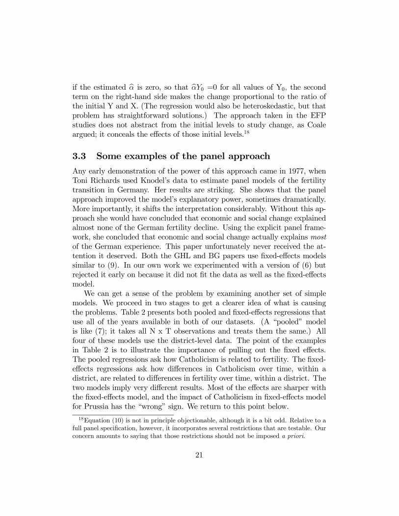
3.3 Some examples of the panel approach

Any early demonstration of the power of this approach came in 1977, whenToni Richards used Knodel’s data to estimate panel models of the fertilitytransition in Germany. Her results are striking. She shows that the panelapproach improved the model’s explanatory power, sometimes dramatically.More importantly, it shifts the interpretation considerably. Without this ap-proach she would have concluded that economic and social change explainedalmost none of the German fertility decline. Using the explicit panel frame-work, she concluded that economic and social change actually explains mostof the German experience. This paper unfortunately never received the at-tention it deserved. Both the GHL and BG papers use fixed-effects modelssimilar to (9). In our own work we experimented with a version of (6) butrejected it early on because it did not fit the data as well as the fixed-effectsmodel.We can get a sense of the problem by examining another set of simple

models. We proceed in two stages to get a clearer idea of what is causingthe problems. Table 2 presents both pooled and fixed-effects regressions thatuse all of the years available in both of our datasets. (A “pooled” modelis like (7); it takes all N x T observations and treats them the same.) Allfour of these models use the district-level data. The point of the examplesin Table 2 is to illustrate the importance of pulling out the fixed effects.The pooled regressions ask how Catholicism is related to fertility. The fixed-effects regressions ask how differences in Catholicism over time, within adistrict, are related to differences in fertility over time, within a district. Thetwo models imply very different results. Most of the effects are sharper withthe fixed-effects model, and the impact of Catholicism in fixed-effects modelfor Prussia has the “wrong” sign. We return to this point below.18Equation (10) is not in principle objectionable, although it is a bit odd. Relative to a

full panel specification, however, it incorporates several restrictions that are testable. Ourconcern amounts to saying that those restrictions should not be imposed a priori.

21

Table 2 also reports three different versions of the R2 goodness-of-fit sta-tistic for the fixed-effects models. The “within” measure is what we obtainif we estimate (8) by OLS. This highlights the model’s ability to explainwithin-district change over time, which is our primary interest. The “be-tween” version of the R2 essentially discards all variation that is within adistrict over time, and runs OLS on the district means. This measure high-lights the model’s ability to explain the differences between the districts. The“overall” R2 is obtained by running OLS on (7), the pooled model. This mea-sure makes no distinction between explanation of variation within districtsas opposed to between districts. Note that in Bavaria, most of the model’s fitarises from its ability to explain cross-sectional differences; the model does arelatively poor job of explaining change over time. Again, the goodness-of-fitstatistic here is not telling us much about what Coale emphasized, which ishow changes in Xs explain changes in fertility.Table 3 reports some examples that are a direct comparison of the EFP

approach, equation (6), to a fixed-effects estimator. Here we have limited thesample for the fixed-effects estimator to the first and last years, to make theresults directly comparable to the EFP approach. (Table 2 reports the samemodel with the full sample). For both Prussia and Bavaria the fixed-effectsestimator fits the data much, much better. This should not be surprising; thefixed-effects estimator places much less structure on the data. Note that thefixed-effects specification noticeably sharpens the impact of urbanization.Our fixed-effects estimators all produce results quite different from those

that come out of either pooled models or simple cross-sections. This im-plies that the fixed-effects, which try to sweep out the effect of unobservedheterogeneity, are playing an important role. What are they? We cannotreally say, because they are proxies for something unobservable. But at amechanical level we can say that in the Prussian data the correlation be-tween the estimated fixed effects and proportions Catholic is about .6. Inthe Bavarian data the correlation is reversed, about -.8. Correlations withproportion urban are much smaller. One way to think of this is to say thatCatholicism is correlated with other factors that in Prussia imply initiallyhigher fertility, and in Bavaria, initially lower fertility than one would expectgiven the observables. Whatever the interpretation, it is clear that failing toaccount for the unobservables yields a model that places misleading weighton Catholicism or any other variable that would be correlated with the un-observables.

22

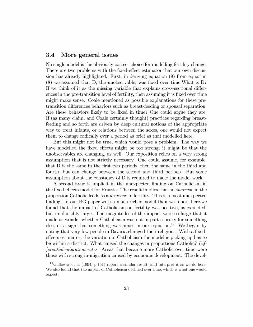
3.4 More general issues

No single model is the obviously correct choice for modelling fertility change.There are two problems with the fixed-effect estimator that our own discus-sion has already highlighted. First, in deriving equation (9) from equation(8) we assumed that D, the unobservable, was fixed over time.What is D?If we think of it as the missing variable that explains cross-sectional differ-ences in the pre-transition level of fertility, then assuming it is fixed over timemight make sense. Coale mentioned as possible explanations for these pre-transition differences behaviors such as breast-feeding or spousal separation.Are these behaviors likely to be fixed in time? One could argue they are.If (as many claim, and Coale certainly thought) practices regarding breast-feeding and so forth are driven by deep cultural notions of the appropriateway to treat infants, or relations between the sexes, one would not expectthem to change radically over a period as brief as that modelled here.But this might not be true, which would pose a problem. The way we

have modelled the fixed effects might be too strong; it might be that theunobservables are changing, as well. Our exposition relies on a very strongassumption that is not strictly necessary. One could assume, for example,that D is the same in the first two periods, then the same in the third andfourth, but can change between the second and third periods. But someassumption about the constancy of D is required to make the model work.A second issue is implicit in the unexpected finding on Catholicism in

the fixed-effects model for Prussia. The result implies that an increase in theproportion Catholic leads to a decrease in fertility. This is a most unexpectedfinding! In our BG paper with a much richer model than we report here,wefound that the impact of Catholicism on fertility was positive, as expected,but implausibly large. The magnitudes of the impact were so large that itmade us wonder whether Catholicism was not in part a proxy for somethingelse, or a sign that something was amiss in our equation.19 We began bynoting that very few people in Bavaria changed their religions. With a fixed-effects estimator, the variation in Catholicism the model is picking up has tobe within a district. What caused the changes in proportions Catholic? Dif-ferential migration rates. Areas that became more Catholic over time werethose with strong in-migration caused by economic development. The devel-

19Galloway et al (1994, p.151) report a similar result, and interpret it as we do here.We also found that the impact of Catholicism declined over time, which is what one wouldexpect.

23

oping areas had initially been mostly Protestant. After including measuresof net migration we found that Catholicism still had the expected positiveimpact on fertility, but the magnitude was less. (We also used proxies forreligiosity, which vary more over time and address the cultural hypothesismore directly.) More generally, results such as these are a warning for themethods we use, and would also be a problem with the approach the EFPused. We always have to ask where the variation over time is coming from.If people do not change their religions, then the variation in the proportionCatholic within a district over time has to be caused by religious differencesin migration, fertility, or mortality. This would be true of any attempt toestimate the impact of a variable that does not change rapidly over time.Using smaller districts may in some cases exacerbate the problem, but thatneed not be the case.Two smaller points are worth noting for their role in the literature. First,

we have treated both of our explanatory variables as exogenous. Some vari-ables important in fertility studies are arguably endogenous and should beapproached as such. In both our study of Bavaria (Brown and Guinnane2002) and one of the GHL team’s works on Prussia (1998a) this issue wasexplored in detail. Second, one sometimes sees the claim that aggregateddata are important because they are the only way to study the impact ofphenomena that are in themselves aggregative. This is simply not true; thebest way to study the effect of, say, a local religious ethos on fertility is touse data at the lowest possible level of aggregation, and to include in thestatistical models variables that measure the religious ethos. This is whatmulti-level modelling is all about. If there is variation across individualsin that environmental variable, this effect be identified with individual-leveldata without the loss of efficiency that comes with aggregation.

4 Conclusions

The Princeton studies have been justly famous since their completion overtwenty years ago. We can thank the Princeton authors, and especially Coale,for setting out an ambitious agenda and devising a methodology that wouldleave us with a broad vision of the fertility transition in Europe. Sincetheir publication the individual monographs, and especially the summarystatement, have been the subject of detailed discussion, praise, and criticism.This paper emphasizes two general statistical problems that affect all of

24

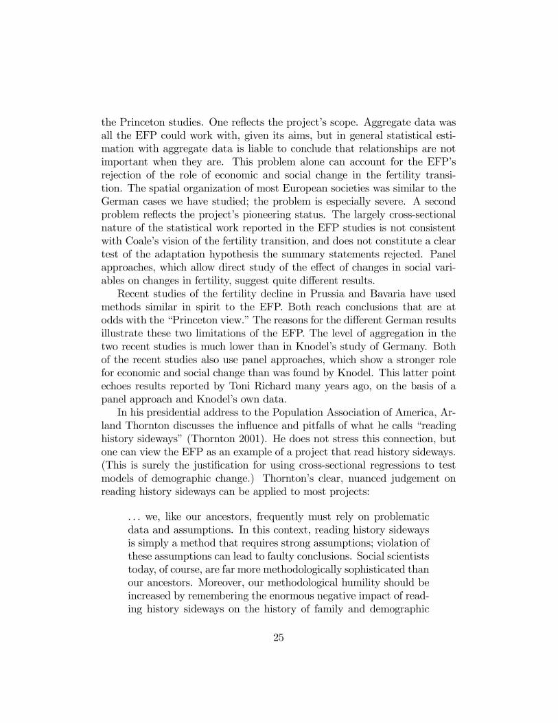
the Princeton studies. One reflects the project’s scope. Aggregate data wasall the EFP could work with, given its aims, but in general statistical esti-mation with aggregate data is liable to conclude that relationships are notimportant when they are. This problem alone can account for the EFP’srejection of the role of economic and social change in the fertility transi-tion. The spatial organization of most European societies was similar to theGerman cases we have studied; the problem is especially severe. A secondproblem reflects the project’s pioneering status. The largely cross-sectionalnature of the statistical work reported in the EFP studies is not consistentwith Coale’s vision of the fertility transition, and does not constitute a cleartest of the adaptation hypothesis the summary statements rejected. Panelapproaches, which allow direct study of the effect of changes in social vari-ables on changes in fertility, suggest quite different results.Recent studies of the fertility decline in Prussia and Bavaria have used

methods similar in spirit to the EFP. Both reach conclusions that are atodds with the “Princeton view.” The reasons for the different German resultsillustrate these two limitations of the EFP. The level of aggregation in thetwo recent studies is much lower than in Knodel’s study of Germany. Bothof the recent studies also use panel approaches, which show a stronger rolefor economic and social change than was found by Knodel. This latter pointechoes results reported by Toni Richard many years ago, on the basis of apanel approach and Knodel’s own data.In his presidential address to the Population Association of America, Ar-

land Thornton discusses the influence and pitfalls of what he calls “readinghistory sideways” (Thornton 2001). He does not stress this connection, butone can view the EFP as an example of a project that read history sideways.(This is surely the justification for using cross-sectional regressions to testmodels of demographic change.) Thornton’s clear, nuanced judgement onreading history sideways can be applied to most projects:

. . . we, like our ancestors, frequently must rely on problematicdata and assumptions. In this context, reading history sidewaysis simply a method that requires strong assumptions; violation ofthese assumptions can lead to faulty conclusions. Social scientiststoday, of course, are far more methodologically sophisticated thanour ancestors. Moreover, our methodological humility should beincreased by remembering the enormous negative impact of read-ing history sideways on the history of family and demographic

25

studies. Thus I can conclude that cross-sectional approaches maybe acceptable for exploratory purposes if we are clear about theassumptions and exceptionally cautious about the results (p.461).

As an exploratory project the EFP was unusually fruitful, ambitious, andinfluential. But if we are “clear about the assumptions and exceptionallycautious about the results,” we will recognize that the summary statementsrely in part on statistical analysis we should no longer trust. This is reasonenough to press on with new sources and new methods.

26

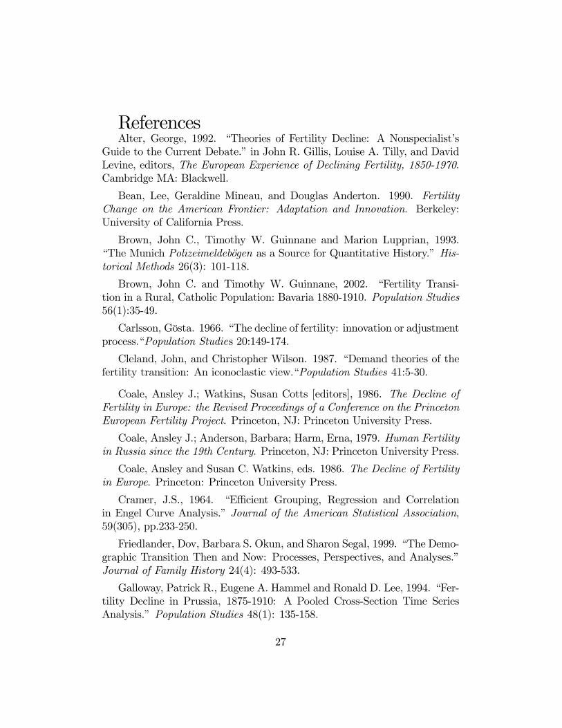
ReferencesAlter, George, 1992. “Theories of Fertility Decline: A Nonspecialist’s

Guide to the Current Debate.” in John R. Gillis, Louise A. Tilly, and DavidLevine, editors, The European Experience of Declining Fertility, 1850-1970.Cambridge MA: Blackwell.

Bean, Lee, Geraldine Mineau, and Douglas Anderton. 1990. FertilityChange on the American Frontier: Adaptation and Innovation. Berkeley:University of California Press.

Brown, John C., Timothy W. Guinnane and Marion Lupprian, 1993.“The Munich Polizeimeldebögen as a Source for Quantitative History.” His-torical Methods 26(3): 101-118.

Brown, John C. and Timothy W. Guinnane, 2002. “Fertility Transi-tion in a Rural, Catholic Population: Bavaria 1880-1910. Population Studies56(1):35-49.

Carlsson, Gösta. 1966. “The decline of fertility: innovation or adjustmentprocess.“Population Studies 20:149-174.

Cleland, John, and Christopher Wilson. 1987. “Demand theories of thefertility transition: An iconoclastic view.“Population Studies 41:5-30.

Coale, Ansley J.; Watkins, Susan Cotts [editors], 1986. The Decline ofFertility in Europe: the Revised Proceedings of a Conference on the PrincetonEuropean Fertility Project. Princeton, NJ: Princeton University Press.

Coale, Ansley J.; Anderson, Barbara; Harm, Erna, 1979. Human Fertilityin Russia since the 19th Century. Princeton, NJ: Princeton University Press.

Coale, Ansley and Susan C. Watkins, eds. 1986. The Decline of Fertilityin Europe. Princeton: Princeton University Press.

Cramer, J.S., 1964. “Efficient Grouping, Regression and Correlationin Engel Curve Analysis.” Journal of the American Statistical Association,59(305), pp.233-250.

Friedlander, Dov, Barbara S. Okun, and Sharon Segal, 1999. “The Demo-graphic Transition Then and Now: Processes, Perspectives, and Analyses.”Journal of Family History 24(4): 493-533.

Galloway, Patrick R., Eugene A. Hammel and Ronald D. Lee, 1994. “Fer-tility Decline in Prussia, 1875-1910: A Pooled Cross-Section Time SeriesAnalysis.” Population Studies 48(1): 135-158.

27

Galloway, Patrick R., Ronald D. Lee, and Eugene A. Hammel 1998a.“Urban versus Rural: Fertility Decline in the Cities and Rural Districts ofPrussa, 1875 to 1910.” European Journal of Population 14:209-264.

Galloway, Patrick R., Ronald D. Lee, and Eugene Hammel, 1998b. "In-fant mortality and the fertility transition: macro evidence from Europe andnew findings for Prussia," in From Death to Births: Mortality Decline andReproductive Change, Washington D.C.: National Academy of Sciences, eds.Cohen, B. and Montgomery, M., Chapter 6, pp. 182-226.

Guinnane, Timothy W., Barbara S. Okun, and James Trussell, 1994.“What do We Know about the Timing of the European Fertility Transi-tion¿‘ Demography 41(1).Knodel, John E, 1974. The Decline of Fertility inGermany, 1871-1939. Princeton, NJ: Princeton, University Press.

Hohenberg, Paul M., Forthcoming, “The Historical Geography of Eu-ropean Cities: An Interpretive Essay,” in V. Henderson and J.F. Thisse,Handbook of Regional and Urban Economics, vol. 4. Amsterdam: ElsevierScience.

King, Gregory, 1977. A solution to the ecological inference problem: Re-covering individual behavior from aggregate data. Princeton: Princeton Uni-versity Press.

Knodel, John, 1988. Demographic behavior in the past: A study of four-teen German village populations in the eighteenth and nineteenth centuries.New York: Cambridge University Press.

Knodel, John and Etienne van de Walle. 1986. “Lessons from the past:Policy implications of historical fertility studies.“in Ansley J. Coale and Su-san C. Watkins, eds. The Decline of Fertility in Europe. Princeton: Prince-ton University Press.

Lesthaeghe, Ron J, 1977. The Decline of Belgian Fertility, 1800-1970.Princeton, NJ: Princeton, University Press.

Lesthaeghe, Ron and Chris Wilson. 1986. “Modes of production, secu-larization, and the pace of fertility decline in western Europe, 1870-1930.“inAnsley J. Coale and Susan C. Watkins, eds. 1986. The Decline of Fertilityin Europe. Princeton: Princeton University Press.

Livi Bacci, Massimo, 1971. A Century of Portuguese Fertility. Princeton,NJ: Princeton University Press.

28

Livi Bacci, Massimo, 1977. A History of Italian Fertility during the LastTwo Centuries. Princeton, NJ: Princeton University Press.

Potter, J. E., C. Schmertmann, and S. M. Cavenaghi. 2003. “Fertilityand Development: Evidence from Brazil.” Demography39(4): 739-762.

Richards, Toni, 1977. “Fertility Decline in Germany: An EconometricAppraisal.” Population Studies 31(3): 537-553.

Teitelbaum, Michael S., 1984. The British Fertility Decline: Demo-graphic Transition in the Crucible of the Industrial Revolution. Princeton,NJ: Princeton University Press.

Thornton, Arland, 2001. “The Developmental Paradigm, Reading His-tory Sideways, and Family Change.” Demography 38(4):449-465.

Van der Walle, Etienne, 1974. The Female Population of France in theNineteenth Century. Princeton, NJ: Princeton University Press.

Watkins, Susan C. 1986. “Conclusions.“in Ansley J. Coale and Susan C.Watkins, eds. 1986. The Decline of Fertility in Europe. Princeton: PrincetonUniversity Press.

29

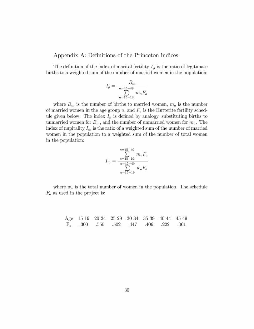
Appendix A: Definitions of the Princeton indices

The definition of the index of marital fertility I g is the ratio of legitimatebirths to a weighted sum of the number of married women in the population:

Ig =Bm

a=45−49Pa=15−19

maFa

where Bm is the number of births to married women, ma is the numberof married women in the age group a, and Fa is the Hutterite fertility sched-ule given below. The index Ih is defined by analogy, substituting births tounmarried women for Bm, and the number of unmarried women for ma. Theindex of nupitality Im is the ratio of a weighted sum of the number of marriedwomen in the population to a weighted sum of the number of total womenin the population:

Im =

a=45−49Pa=15−19

maFa

a=45−49Pa=15−19

waFa

where wa is the total number of women in the population. The scheduleFa as used in the project is:

Age 15-19 20-24 25-29 30-34 35-39 40-44 45-49Fa .300 .550 .502 .447 .406 .222 .061

30

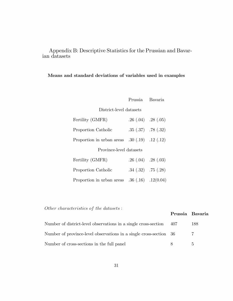
Appendix B: Descriptive Statistics for the Prussian and Bavar-ian datasets

Means and standard deviations of variables used in examples

Prussia Bavaria

District-level datasets

Fertility (GMFR) .26 (.04) .28 (.05)

Proportion Catholic .35 (.37) .78 (.32)

Proportion in urban areas .30 (.19) .12 (.12)

Province-level datasets

Fertility (GMFR) .26 (.04) .28 (.03)

Proportion Catholic .34 (.32) .75 (.28)

Proportion in urban areas .36 (.16) .12(0.04)

Other characteristics of the datasets :Prussia Bavaria

Number of district-level observations in a single cross-section 407 188

Number of province-level observations in a single cross-section 36 7

Number of cross-sections in the full panel 8 5

31

TABLE 1

The effects of aggregation

Sample ConstantProportionCatholic

ProportionUrban

AdjustedR-square

Prussia,1880districts

.256(.003)

.062(.003)

-.007(.007)

.44

Prussia,1880,provinces

.254(.011)

.072(.012)

-.015(.026)

.53

Bavaria,1880,districts

.226(.009)

.081(.009)

-.011(-.39)

.36

Bavaria,1880,provinces

.261(.045)

.083(.031)

-.390(.399)

.50

Prussia,1910,districts

.229(.003)

.093(.004)

-.103(.008)

.66

Prussia,1910,provinces

.252(.016)

.089(.016)

-.152(.032)

.66

Bavaria,1910,districts

.189(.008)

.102(.009)

-.084(.021)

.50

Bavaria,1910,provinces

.193(.034)

.122(.037)

-.214(.223)

.60

Note: OLS estimates, standard errors in parentheses.

Source: Estimated from Prussian and Bavarian datasets described in thetext.

32

TABLE 2

Fixed-effects and Pooled Regressions of Panel Fertility Data

Type of regression Constant Catholic Urban R2

(1)Prussia, districtswith fixed effects1875-1910

.506(.009)

-.478(.027)

-.265(.010)

.308.401.285

(2)Prussia, districts,pooled regression1875-1910

.252(.001)

.070(.002)

-.053(.003)

.440

(3)Bavaria, districtswith fixed effects1880-1910

.119(.094)

.216(.121)

-.062(.015)

.033

.444

.380

(4)Bavaria, districts,pooled regression1880-1910

.215(.004)

.088(.004)

-.035(.011)

.381

Note: Standard errors in parentheses. The three values of R2 in models(1) and (3) are the within, between, and overall measures discussed in thetext.

Source: Estimated from the Prussian and Bavarian datasets described inthe text.

33

TABLE 3

Modelling changes in fertility

State and type of regression Constant Catholic Urban R2

(1)Pr ussia, percent changes1875 to 1910 N=394

20.333(.893)

-.003(.002)

0.034(.019)

.015

(2)Bavaria, percent changes1880 to 1910 N=135

17.47(1.534)

.020(.020)

.009(.002)

.153

(3)Pr ussia: fixed effects estimator1875 and 1910 N=814

.546(.023)

-.513(.067)

-.379(.027)

.440

.345

.193

(4)Bavaria, fixed effects estimator1880 and 1910 N=138

.215(.162)

.104(.207)

-.201(.029)

.263

.410

.378

Note: Standard errors in parentheses.The three values of R2 in models (3)and (4) are the within, between, and overall measures discussed in the text.

Source: Estimated from the Prussian and Bavaria datasets discussed inthe text.

34