TWISTOR CR MANIFOLD BY NON-RIEMANNIAN CONNECTIONS by Ho Chi Low B. Sc. in Mathematics, Hong Kong, 2011 M. Phil. in Mathematics, Hong Kong, 2013 Submitted to the Graduate Faculty of the Dietrich School of Arts and Sciences in partial fulfillment of the requirements for the degree of Doctor of Philosophy University of Pittsburgh 2020

Welcome message from author
This document is posted to help you gain knowledge. Please leave a comment to let me know what you think about it! Share it to your friends and learn new things together.
Transcript

TWISTOR CR MANIFOLD BY
NON-RIEMANNIAN CONNECTIONS
by
Ho Chi Low
B. Sc. in Mathematics, Hong Kong, 2011
M. Phil. in Mathematics, Hong Kong, 2013
Submitted to the Graduate Faculty of
the Dietrich School of Arts and Sciences in partial fulfillment
of the requirements for the degree of
Doctor of Philosophy
University of Pittsburgh
2020

UNIVERSITY OF PITTSBURGH
DIETRICH SCHOOL OF ARTS AND SCIENCES
This dissertation was presented
by
Ho Chi Low
It was defended on
3/19/2020
and approved by
G. A. J. Sparling, Ph. D., Associate Professor
J. DeBlois, Ph. D., Associate Professor
P. Hajlasz, Ph. D., Professor
C. LeBrun, Ph. D., Professor
Dissertation Director: G. A. J. Sparling, Ph. D., Associate Professor
ii

TWISTOR CR MANIFOLD BY NON-RIEMANNIAN CONNECTIONS
Ho Chi Low, PhD
University of Pittsburgh, 2020
Developed by LeBrun, twistor CR manifold is a 5-dimensional CR manifold foliated by
Riemann spheres. The CR structure is determined by both the complex structure on the
Riemann sphere and the geometric information of the space of leaves, which is a 3-manifold
endowed with a conformal class and a trace-free symmetric(1,1)-tensor.
When the (1,1)-tensor is zero, the twistor CR structure of zero torsion, named as the rival
CR structure on LeBrun’s paper “Foliated CR Manifolds”, is obtained. These CR structures
are embeddable to a complex 3-manifold if and only if the metric tensor is conformal to a
real analytic metric.
We try to understand twistor CR structures through the corresponding Fefferman metric
defined on the canonical circle-bundle of the given CR manifold. The conformal class of the
Fefferman metric is preserved over the choice of contact forms of the CR structure, so it
makes possible to classify CR structures by the confomal curvature tensor of the Fefferman
metric.
Our main results include representing the Weyl tensor of the Fefferman metric in terms
of the Cotton tensor on the 3-manifold when the twistor CR structure is of zero torsion.
Moreover, we obtain conditions for vanishing Weyl tensor when the space of leaves is under
a flat metric.
iii
TABLE OF CONTENTS
PREFACE . . . . . . . . . . . . . . . . . . . . . . . . . . . . . . . . . . . . . . . . . vi
1.0 INTRODUCTION . . . . . . . . . . . . . . . . . . . . . . . . . . . . . . . . 1
1.1 Overview . . . . . . . . . . . . . . . . . . . . . . . . . . . . . . . . . . . . 1
1.2 Cauchy-Riemann geometry . . . . . . . . . . . . . . . . . . . . . . . . . . 4
1.3 Embeddable CR manifolds . . . . . . . . . . . . . . . . . . . . . . . . . . . 6
1.4 Tanaka-Webster connection . . . . . . . . . . . . . . . . . . . . . . . . . . 8
1.5 The Fefferman bundle and the Fefferman metric . . . . . . . . . . . . . . . 12
2.0 TWISTOR CR MANIFOLD OF HAMILTONIAN DISTRIBUTION 16
2.1 The twistor CR manifold N of (M , g) . . . . . . . . . . . . . . . . . . . . 16
2.2 The rational parametrization of N and N . . . . . . . . . . . . . . . . . . 18
2.3 The Levi form of (N ,D) and (N,D) . . . . . . . . . . . . . . . . . . . . . 21
2.4 CR structure on the sphere bundle of M . . . . . . . . . . . . . . . . . . . 24
2.5 Embedding into complex 3-manifold . . . . . . . . . . . . . . . . . . . . . 26
3.0 CR STRUCTURE BY AFFINE CONNECTIONS . . . . . . . . . . . . 29
3.1 Weyl connection on (M, g) . . . . . . . . . . . . . . . . . . . . . . . . . . . 29
3.2 Metric connection with torsion . . . . . . . . . . . . . . . . . . . . . . . . 32
3.3 The trace-free second fundamental form . . . . . . . . . . . . . . . . . . . 38
4.0 FEFFERMAN METRIC (I) . . . . . . . . . . . . . . . . . . . . . . . . . . 42
4.1 The local model of D(w) . . . . . . . . . . . . . . . . . . . . . . . . . . . . 42
4.2 Fefferman bundle and Fefferman metric . . . . . . . . . . . . . . . . . . . . 50
4.3 Further results when M is flat . . . . . . . . . . . . . . . . . . . . . . . . . 54
5.0 FEFFERMAN METRIC (II) . . . . . . . . . . . . . . . . . . . . . . . . . 62
iv

5.1 Change of coordinates on N . . . . . . . . . . . . . . . . . . . . . . . . . . 62
5.2 The local model of D(w): general case . . . . . . . . . . . . . . . . . . . . 68
5.3 The scalar curvature formula . . . . . . . . . . . . . . . . . . . . . . . . . 76
5.4 The Chern-Moser curvature tensor . . . . . . . . . . . . . . . . . . . . . . 82
5.5 Fefferman metric in the general setting . . . . . . . . . . . . . . . . . . . . 86
6.0 WEYL CURVATURE TENSOR (I) . . . . . . . . . . . . . . . . . . . . . 90
6.1 Properties of the Weyl tensor . . . . . . . . . . . . . . . . . . . . . . . . . 90
6.2 Components of the Weyl tensor involving T . . . . . . . . . . . . . . . . . 92
6.3 The twistor CR manifold of zero torsion . . . . . . . . . . . . . . . . . . . 97
7.0 WEYL CURVATURE TENSOR (II) . . . . . . . . . . . . . . . . . . . . . 101
7.1 The almost w-linear components . . . . . . . . . . . . . . . . . . . . . . . 101
7.2 The vanishing of the Weyl tensor . . . . . . . . . . . . . . . . . . . . . . . 108
7.3 The general solution . . . . . . . . . . . . . . . . . . . . . . . . . . . . . . 120
APPENDIX A. SOLUTION TO EQUATION (7.31) . . . . . . . . . . . . . . 125
APPENDIX B. PROOF OF THEOREM 6.2 . . . . . . . . . . . . . . . . . . . 137
APPENDIX C. COMPUTATIONAL MODEL IN MATLAB . . . . . . . . . 162
BIBLIOGRAPHY . . . . . . . . . . . . . . . . . . . . . . . . . . . . . . . . . . . . 189
v

PREFACE
I would like to express my deepest gratitude to every professor in the dissertation committee.
In particular, thank you very much to Professor LeBrun for his wonderful work on the subject
of the twistor CR manifold, combined with his advice and suggestions on our research. Last
but not least, special thanks to Professor Sparling as this article would have never appeared
without his help.
vi

1.0 INTRODUCTION
We would begin with an overview of the thesis, followed by background knowledge in CR
geometry which are essential to the research. The background materials are adopted mainly
from early chapters of [3] and [4]. Meanwhile, the books [7] and [19] provides fundamental
concepts in differential geometry.
1.1 OVERVIEW
The concept of twistor CR manifold originates from Penrose’s work on the twistor theory
[14]. The twistor space (T) of the four dimensional Minkowski space (M) is defined to be a
4-dimensional complex vector space such that every null twistor inside T could represent a
null geodesic on M. The space of null geodesics would then form a hypersurface inside the
projective twistor space (P (T)), which is diffeomorphic to CP 3.
A natural CR structure is then introduced to the space of null geodesics by Penrose on [15].
On that article, the incident correspondence is defined to relate points of M to null twistors
on T. In this approach, every equivalence class [W ] of null twistors on P (T), outside an
exceptional set I , could be identified with a unique null geodesic on the Minkowski space.
The space of null geodesics, denoted by P (T0)\I , carries a natural CR structure from P (T).
1

As a generalization, over a globally hyperbolic Lorentzian 4-manifold, the space of null
geodesics could be equipped with a CR structure depending on the choice of a hypersurface
which meets every null geodesic on the manifold [15].
LeBrun developed the concept of twistor CR manifold much in his work: [8], [9] and [10].
On [10], LeBrun proves that a twistor CR manifold in 5 dimension, is exactly a foliation
of Riemann spheres equipped with a non-degenerate CR structure. The space of leaves is
a real 3-manifold M . Moreover, the CR structure itself can be characterized by the first
and second fundamental forms of M , which represent a prescribed conformal class and a
prescribed trace-free symmetric (1, 1)-tensor respectively.
When M is a hypersurface of the twistor space of a self-dual Riemannian 4-manifold, which
happens to be a complex 3-manifold, the above first and second fundamental forms become
the conformal part of the first and second fundamental forms of M in their usual definitions
correspondingly under the twistor construction.
A particular class of twistor CR manifolds can be obtained if the second fundamental form
vanishes. It is named the rival CR structure on [10] and elaborated in details on [9]. LeBrun
also shows that this special twistor CR manifold of a smooth 3-manifold M equipped with the
metric g, is embeddable to a complex 3-manifold if and only if its conformal class [g] contains
a real analytic metric on M . This property doesn’t hold in general for a twistor CR manifold.
The rival CR structure is also named as the twistor CR manifold of Hamiltonian distribution
or that of zero torsion in this article.
Our research initiates from LeBrun’s work on the twistor CR manifold and borrow many of
his definitions and results as foundations. We try to develop from his work and classify these
CR structures by investigating the Fefferman metric on the Fefferman bundle. Since the
conformal class of the Fefferman metric of a CR structure is a CR invariant, the conformal
curvature of the Fefferman metric conveys information of the geometry of the CR structure.
2

The theoretical tools we adopt, come from the theory of CR geometry and that of differential
geometry. We build the local model of the twistor CR structure, with or without torsion,
and analyze the CR structure in local variables in order to capture properties of the Weyl
tensor. This process would demand a lot of computational work, so computer programming
in Matlab [12] is also an essential part in our research.
The remaining part of the beginning chapter is a summary of definitions and theorems in CR
geometry. Then, in Chapter 2, we will elaborate LeBrun’s work on the twistor CR manifold
of Hamiltonian distribution extensively and try to translate his concepts and results to our
local model of twistor CR structures. The second fundamental form, which is equivalent to
the trace-free torsion tensor of a metric connection on the 3-manifold [8], is introduced in
Chapter 3, where we also complete the construction of the local model of the twistor CR
structure (with torsion).
Chapter 4 and 5, combined as one unit, contains the theoretical picture of both the Tanaka-
Webster connection and the Fefferman metric to support the computational model. The
Weyl curvature tensor of the twistor CR structure, as the key subject in our research, will
be discussed in Chapter 6 and 7, followed by the main findings.
By characterizing the coefficients of the Weyl tensor, we could obtain important results such
as representing the Weyl tensor of the Fefferman metric in terms of the Cotton tensor on the
3-manifold when the twistor CR structure is of zero torsion. Moreover, we obtain conditions
for vanishing Weyl tensor when the space of leaves is under a flat metric.
3

1.2 CAUCHY-RIEMANN GEOMETRY
Let N be a smooth manifold and L be a smooth complex distribution on N . We define L
to be the complex conjugation of L in CTN .
Definition. L is a CR structure on N if both conditions (1) and (2) are satisfied.
(1) L ∩ L = 0.
(2) L is integrable: for any open set U on N , smooth sections of L over U
are involutive. That is,[Γ∞(U,L), Γ∞(U,L)
]⊆ Γ∞(U,L).
We specify that L is the holomorphic bundle and L is the antiholomorphic bundle of the CR
structure. If L is of complex rank ν and N is a manifold of real dimension 2ν + d, then we
say L is of type (ν, d). ν is called the CR dimension, and d the CR codimension of L. When
d = 1, L is of hypersurface type.
The pair (N,L) is then called a CR manifold (of type (n, d)). Given that N ′ is another CR
manifold equipped with the CR structure L′, a smooth function f from N to N ′ is a CR
map whenever df(L) ⊆ L′. Moreover, we say that N is CR equivalent (or CR isomorphic)
to N ′ when there is a diffeomorphism f : N → N ′ such that df(L) = L′.
The real subbundle of rank 2ν, H(N), consists of tangent vectors to N in the form of X+X,
where X is on L. H(N) is named the Levi distribution of the CR structure.
There is a natural almost complex structure (J) defined on H(N). We first impose that
J(X) = iX and J(X) = −iX when X is a holomorphic vector. Then J is characterized by
J(X +X
)= i(X −X
)for X ∈ L.
Assume that the CR manifold N is always of hypersurface type (d = 1) from here.
4
Definition. A pseudo-hermitian structure of N is a smooth real 1-form α annihilating
H(N). The Levi form L associated with α is a complex bilinear map defined by
L : L× L→ C, L(X, Y ) = − idα(X, Y )
for X on L and Y on L.
The 1-form α could be replaced by fα for any non-vanishing function f on N . In this case,
we let L1 be the Levi form associated with fα. It makes
L1(X, Y ) = f · L(X, Y ) for any X ∈ L, Y ∈ L.
We say that the Levi form L is non-degenerate, if for any v on L, there is a vector w on L
such that L(v, w) 6= 0. Moreover, we say that L is positive definite when L(v, v) > 0 for any
nonzero vector v on L.
If L is non-degenerate, then any other Levi form of L is also non-degenerate. So we could
say that the CR structure L is non-degenerate when any of its Levi forms is non-degenerate.
In this case, we also say α is a contact form on N since α ∧ (dα)n 6= 0 at every point of N .
Definition. Let N be a CR manifold of hypersurface type. Suppose L is the CR structure
of N and L is non-degenerate.
(1) N is strictly pseudoconvex, if for some choice of pseudo-hermitian form α,
its associated Levi form is positively definite.
(2) N is anticlastic if the Levi form, associated to any pseudo-hermitian form,
consists of eigenvalues of opposite signs.
5

1.3 EMBEDDABLE CR MANIFOLDS
A huge class of CR manifolds is the collection of CR submanifolds of Cm. It means that
the manifold N is a submanifold of Cm and it inherits a CR structure from the standard
complex structure (J0) of Cm. The Levi distribution is the J0-invariant subspace of TN , i.e.
H(N) = TN ∩ J0(TN).
We define the holomorphic bundle and the antiholomorphic bundle of the CR structure by
T 1,0N = T 1,0Cm ∩ CTN and T 0,1N = T 0,1Cm ∩ CTN
In general, an embedded manifolds in Cm obtains a natural CR structure from Cm as long as
the real dimension of H(N) keeps constant. We would mainly look at the real hypersurface
in Cm since they correspond to the case that CR codimension is 1.
An example of real hypersurface is the graph of function.
Let z = x + iy be the first coordinate of Cm and let w = (w1, · · · , wm−1) be the remaining
complex coordinates. We define a smooth function h : R × Cm−1 → R by h = h(x,w). Its
graph is a hypersurface M =
(x+ iy, w) ∈ Cm | y = h(x,w)
. Furthermore, we assume
h(0, 0) = 0,∂h
∂x=
∂h
∂wj=
∂h
∂wj= 0
at (0, 0) for j = 1, · · · ,m− 1.
Since the direct sum of TM and J0(TM) spans the entire Cm, we get
dimR(H(M)) = dimR(TM) + dimR(J0(TM))− dimR(Cm) = 2m− 2.
So the CR codimension of M is 1, equal to its geometric codimension. In general, we say that
a CR submanifold of Cm is generic if its geometric codimension equal to its CR codimension.
6

The holomorphic bundle T 1,0M of the real hypersurface M is spanned by the vectors
Tj =∂
∂wj+
2i
(1− ihx)∂h
∂wj
∂
∂z
at (x+ iy, w) for j = 1, · · · ,m− 1. The antiholomorphic bundle is spanned by
Tj =∂
∂wj− 2i
(1 + ihx)
∂h
∂wj
∂
∂z.
A pseudo-hermitian structure of M could be found by
θ =(1− ihx)
2dz +
(1 + ihx)
2dz − i ∂h
∂wjdwj + i
∂h
∂wjdwj.
All real analytic CR manifolds are locally embeddable to Cm for some m. We quote the real
analytic embedding theorem (Theorem 1.1) here. Readers may refer to Chapter 11 of [3] for
its proof and more details.
Definition. A CR manifold N is real analytic if N is a real analytic manifold, and the CR
structure L is a real analytic subbundle of the complex tangent bundle of N .
Theorem 1.1. Suppose N is a real analytic CR manifold of real dimension 2m− d. Let L
be its CR structure, and the CR codimension of L be d ≥ 1. Then, given any point p on
N , there is a neighborhood U of p such that the CR structure (U,L) is CR equivalent to a
generic real analytic CR submanifold of Cm with CR codimension equal to d.
If φ = (z1, · · · , zm) defines such a local embedding from N to Cm, then all the component
functions zj’s of φ must be CR functions (complex-valued CR maps). That is, Y (zj) = 0 for
any vector field Y in L.
7
1.4 TANAKA-WEBSTER CONNECTION
Let N be a CR manifold of dimension 5. The CR structure of N is denoted by D, which also
represents its antiholomorphic bundle. Over the course of the thesis, we would like to reserve
any capital letter D (or D) to represent the T 0,1-part of the CR structure. The holomorphic
bundle would be denoted by D or D.
Suppose α is a pseudo-hermitian structure on N . When dα is non-degenerate, there exists
a unique tangent vector field T , such that α(T ) = 1 and ιTdα = 0 at every point. We may
call T the characteristic vector field associated with α. If α is also a contact form, then T is
the Reeb vector field associated with α.
Also, we let T1, T2 be a basis for D. So T1 = T 1 and T2 = T 2 is a basis for D. The collection
of T1, T2, T1, T2 and T form a moving frame for CTN .
Under our notation, the Levi form L of α maps from D×D to C. Let hαβ = L(Tα, Tβ). We
let h =[hαβ]
be a 2× 2 matrix and denote its inverse by h−1 =[hαβ], i.e.∑
β
hαβ · hβσ = δασ.
h is hermitian so that hαβ = hβα and hβα = hαβ.
Definition. The Webster metric g associated with the pseudo-hermitian structure α, is a
pseudo-Riemannian metric on N defined by
g(T, T ) = 1, g(Tα, Tβ) = hαβ and g(Tα, Tβ) = g(Tα, Tβ) = g(Tα, T ) = g(Tβ, T ) = 0,
for α, β = 1, 2.
8
The Webster metric is Riemannian if the CR structure is strictly pseudo-convex and the
metric itself is defined by a positive definite Levi form. However, since our work is on
anticlastic CR manifolds, the signature of g would be (+ + +−−).
Rather than the Levi-Civita connection, we study the Tanaka-Webster connection of g
referring to Webster’s paper [20] or in Chapter 1 of [4].
Definition. The Tanaka-Webster connection ∇ associated with α, is an affine connection
on N uniquely defined by the following properties.
(1) ∇ is a metric connection with respect to g.
(2) ∇XTα belongs to T 1,0N , and ∇XTβ belongs to T 0,1N , for any X on CTN .
(3) ∇XT = 0 for any X on CTN .
(4) Let tor be the torsion tensor of ∇, tor(X, Y ) = ∇XY −∇YX − [X, Y ].
Then, tor(Tα, Tβ) belongs to the linear span of T .
(5) Let τ be the operator τ(X) = tor(T,X). Then, τ sends T 1,0N to T 0,1N
and vice versa.
By the definition above, for m,n = 1, 2, we let
∇TmTn = ΓkmnTk, ∇TmTn = ΓkmnTk and ∇TTn = Γk0nTk.
The coefficients of the Tanaka-Webster connection are then given by
Γkmn = hlk
(dhnl(Tm)− g
(Tn, [Tm, Tl]
)),
Γkmn = hlk · g([Tm, Tn], Tl
),
Γk0n = hlk · g([T, Tn], Tl
).
(1.1)
9
Let R be the curvature tensor field of the Tanaka-Webster connection ∇. We follow the
usual definition that R(Y, Z)X = ∇Y∇ZX −∇Z∇YX −∇[Y,Z]X. In our study, we assume
that Y lies on D and Z lies on D. In particular,
R(Tk, Tl)Tm = ∇Tk∇TlTm −∇Tl
∇TkTm −∇[Tk,Tl]Tm.
Let R(Tk, Tl)Tm = Rmnkl Tn. Explicitly,
Rmnkl = dΓnlm(Tk)− dΓnkm(Tl)− ΓpkmΓnlp + Γp
lmΓnkp + Γp
lkΓnpm − Γp
klΓnpm + 2ihklΓ
n0m. (1.2)
As a remark, the Christoffel symbol Γpkl
equals (Γpkl
).
The lower index of R is defined by Rmnkl = g(R(Tk, Tl)Tm, Tn
)= Rm
pkl hpn.
We also define the Ricci tensor (ric) and the scalar curvature (ρ) specific to the Tanaka-
Webster connection on N . These two variables are more often named as the pseudo-hermitian
Ricci tensor and the pseudo-hermitian scalar curvature respectively. To keep everything
simple, we would call them by the shorter names. They are defined by
ric(Tλ, Tµ) = Rλµ = Rλααµ and ρ = hµλ ·Rλµ. (1.3)
The raise-index of ric becomes an operator from D to itself. We would call it by ric].
ric](Tm) = RnmTn with Rn
m = Rmp · hpn.
The Chern-Moser curvature tensor field (C) is the analogue of the Weyl curvature tensor in
Riemannian geometry. We would introduce it briefly here, and for more details, readers may
refer to [2] and [20]. Let ν be the CR dimension of D. We have
C(Tk, Tl)Tm = R(Tk, Tl)Tm −1
ν + 2
(hkl ric](Tm) + hml ric](Tk) +Rkl Tm +Rml Tk
)+
ρ
(ν + 1)(ν + 2)
(hkl Tm + hml Tk
).
10

Writing C(Tk, Tl)Tm = Cmnkl Tn and ν = 2, we have
Cmnkl = Rm
nkl−
1
4
(Rnm hkl+Rn
k hml+Rkl δmn+Rml δkn
)+ρ
12
(hkl δmn+hml δkn
). (1.4)
The lower-index of C is then given by Cmnkl = g(C(Tk, Tl)Tm, Tn
). Explicitly,
Cmnkl = Rmnkl −1
4
(Rmnhkl +Rklhmn +Rmlhkn +Rknhml
)+
ρ
12
(hmnhkl + hmlhkn
). (1.5)
The Chern tensor behaves similarly to the Weyl tensor in the way that if it remains
unchanged when the pseudo-hermitian form α is replaced by another pseudo-hermitian form.
Proposition 1.2. Let α be a pseudo-hermitian form of D, and C be the (1,3)-Chern
tensor of the Tanaka-Webster connection of α. Suppose α = e2fα for some smooth real-
valued function f on N , and C is the (1,3)-Chern tensor of the Tanaka-Webster connection
of α. Then, C = C on N .
If we fix the basis of T1, T2, T1, T2 for the Levi distribution D⊕D, then the above theorem
means C(Tk, Tl)Tm = C(Tk, Tl)Tm. Explicitly, Cmn
kl = Cmnkl and Cmnkl = e2f Cmnkl for
every m, n, k and l.
11
1.5 THE FEFFERMAN BUNDLE AND THE FEFFERMAN METRIC
The approach from [11] is adopted to construct the Fefferman bundle and the Fefferman
metric of the CR manifold N . We are in the case that the CR dimension ν is 2, so the
Fefferman bundle is of real dimension 2ν + 2 = 6. For better understanding on the subject
of Fefferman metrics, especially when ν = 1, readers may also refer to [13].
A pseudo-hermitian structure α on N is fixed in the following so that the Levi-form (L, hαβ)
and the Tanaka-Webster connection (∇) are well-defined.
Consider the moving frameT1, T2, T1, T2, T
for TN . Let
θ1, θ2, θ1, θ2, α
be the dual
coframe. It means that θi(Tj) = θi(Tj) = δij, θi(Tj) = θi(Tj) = α(Tj) = α(Tj) = 0 and
α(T ) = 1. We say that a 1-form η on N is of type (0, 1) if
η(T ) = η(Tj) = 0 for j = 1, 2.
As the complement, we say that η is of type (1, 0) if
η(Tj) = 0 for j = 1, 2.
Our notation of differential forms of type (0, 1) and type (1, 0), is adopted from [3]. Note
that the pseudo-hermitian structure α is of type (1, 0) by default.
The connection forms of the Tanaka-Webster connection, are the 1-forms ωnm on N with
m,n = 1, 2, defined by ∇Tm = ωnm ⊗ Tn. In terms of the Christoffel symbols,
ωnm = Γnkm θk + Γnkm θ
k + Γn0m α. (1.6)
We then define the canonical bundle K(N) = Λ3,0(N) to be the complex line bundle of
differential forms of type (3, 0) on N . For example, K(N) is locally spanned by α∧ θ1 ∧ θ2.
We then let C(N) be the quotient space,
C(N) =(K(N)− 0
)/R+.
It means that we exclude the zero section of K(N), and then every nonzero element ε1 in
K(N) is identified with k ε1 for any positive real number k.
12
C(N) defines a principal S1-bundle over N and it is called the Fefferman bundle of N . Let
π : C(N)→ N be the projection map. Also, we introduce γ to be the real parameter of S1
on C(N), which represents the equivalence class of eiγ α ∧ θ1 ∧ θ2.
The collectionT1, T2, T1, T2, T,
∂∂γ
forms a basis for the complex tangent bundle of C(N).
Corresponding to this basis, we define a 1-form σ on C(N) by (ν = 2)
σ =1
ν + 2
[dγ + π∗
(iωmm −
i
2hnmdhmn −
1
4(ν + 1)ρ α)].
The Fefferman metric (associated with α) of the CR manifold N , is a pseudo-Riemannian
metric on C(N) given by
F = π∗(g|D⊕D
)+ 2(π∗α σ
). (1.7)
The tensor g|D⊕D is restriction of the Webster metric, 2hαβ θα θβ. Here the symmetric
product between two (0, 1)-tensors A and B is obtained by
AB =1
2
(A⊗B +B ⊗ A
).
The conformal class of the Fefferman metric is a CR invariant.
Theorem 1.3. [11] Let N be a CR manifold and Fα be the Fefferman metric on C(N)
associated with the pseudo-hermitian structure α. Suppose that the Levi form of N is
non-degenerate. Let α = e2fα be another pseudo-hermitian structure, for some real function
f on N . Let Fα be the corresponding Fefferman metric. Then, Fα = e2fπFα.
Denote the Levi-Civita connection of F on C(N) by ∇. We use the notation that u1 = T1,
u2 = T1, u3 = T2, u4 = T2, u5 = T and u6 = ∂∂γ
for simplicity.
Let ∇uiuj = Γkijuk and [ui, uj] = Akijuk. The Koszul formula gives,
2F(∇uiuj, uk
)= ui
(F (uj, uk)
)+ uj
(F (ui, uk)
)− uk
(F (ui, uj)
)−F([ui, uk], uj
)− F
([uj, uk], ui
)+ F
([ui, uj], uk
).
.
13
So, we have
Γij,k = F(∇uiuj, uk
)=
1
2
[dFjk(ui) + dFik(uj)− dFij(uk)−AlikFjl −AljkFil +AlijFkl
]and also
Γkij =1
2F kl[dFjl(ui) + dFil(uj)− dFij(ul)−ApilFjp −A
pjlFip +ApijFlp
]. (1.8)
Let R be the Riemann curvature tensor of ∇ on C(N).
R(ui, uj)uk = ∇ui∇ujuk − ∇uj∇uiuk − ∇[ui,uj ]uk
=(dΓljk(ui)− dΓlik(uj) + ΓpjkΓ
lip − ΓpikΓ
ljp −A
pijΓ
lpk
)ul
We write R(ui, uj)uk = Rlijkul, and it means
Rlijk = dΓljk(ui)− dΓlik(uj) + ΓpjkΓ
lip − ΓpikΓ
ljp −A
pijΓ
lpk. (1.9)
Contracting with the metric F , we also have
Rijkl = F(R(ui, uj)uk, ul
)= Fml
(dΓmjk(ui)− dΓmik(uj) + ΓpjkΓ
mip − ΓpikΓ
mjp −A
pijΓ
mpk
). (1.10)
Accordingly, the Ricci tensor are defined by
Rij = Ric(ui, uj) = Rkkij = F klRkijl. (1.11)
And the scalar curvature is given by
S = F npRnp = F npFmqRmnpq. (1.12)
Let Ric] be the raise-index of Ric. We let Ric](ui) = Rjiuj so Rj
i = RikFkj.
Using J. M. Lee’s theorem, the term S could be found easily by the scalar curvature of the
Tanaka-Webster connection.
Theorem 1.4. [11] The scalar curvature of the Fefferman metric F is given by
S =2ν + 1
ν + 1ρ,
where ρ is the scalar curvature of the Tanaka-Webster connection, and ν is the CR dimension
of the underlying CR structure.
14

In terms of the connection forms of ∇ on C(N), we have
∇ui = ωji ⊗ uj for any i, j = 1, · · · , 6. (1.13)
We may also find out the coefficients of R using the connection forms above. We obtain
R(ui, uj
)um = 2Ωn
m(ui, uj)un with Ωnm = dωnm − ωkm ∧ ωlk. In other words,
Rlijk = 2
(dωlk − ω
pk ∧ ω
lp
)(ui, uj
). (1.14)
As a remark, we will always use the convention that φ ∧ ψ =1
2
(φ ⊗ ψ − ψ ⊗ φ
)and
dφ(u, v) =1
2
[u(φ(v)
)− v(φ(u)
)− φ([u, v]
)]for any 1-forms φ and ψ.
The Weyl curvature tensor of ∇ in terms of a (1, 3)-tensor, is defined by
W(ui, uj)uk = R(ui, uj)uk +1
4F (ui, uk)Ric](uj)−
1
4F (uj, uk)Ric](ui)
+1
4Ric(ui, uk)uj −
1
4Ric(uj, uk)ui +
S
20
(F (uj, uk)ui − F (ui, uk)uj
).
for every ui, uj and uk. Let W(ui, uj)uk =W lijkul. We have
W lijk = Rl
ijk +1
4RljFik −
1
4RliFjk +
1
4Rikδjl −
1
4Rjkδil +
S
20
(Fjkδil − Fikδjl
). (1.15)
The lower-index of W is then defined by Wijkl = F(W(ui, uj)uk, ul
), with
Wijkl = Rijkl −1
4RilFjk −
1
4RjkFil +
1
4RikFjl +
1
4RjlFik +
S
20
(FilFjk − FikFjl
). (1.16)
The Weyl tensor shares the same symmetries with the Riemann tensor R, including
Wijkl = −Wjikl = −Wijlk, Wijkl =Wklij, and Wijkl +Wjkil +Wkijl = 0.
Moreover, W is trace-free because WijklFil = 0.
As a remark. W is conformally invariant with respect to the metric. That is, if the metric
F is replaced by e2λF , then the (1,3)-Weyl tensor remains the same, and the (0,4)-Weyl
tensor of e2λF becomes e2λW . Moreover, F is conformally flat if and only if the Weyl tensor
vanishes.
15

2.0 TWISTOR CR MANIFOLD OF HAMILTONIAN DISTRIBUTION
On LeBrun’s paper [9], for every 3-dimensional Riemannian manifold M equipped with the
metric g, the twistor CR manifold of (M, g) is constructed by the Hamiltonian distribution
on the complex cotangent bundle of M . This definition of a 5-dimensional twistor CR
manifold is invariant over the conformal class of g.
The twistor CR manifold mentioned in this chapter, refers to the twistor CR structures of
zero torsion in later context.
2.1 THE TWISTOR CR MANIFOLD N OF (M , g)
Let M be a 3-dimensional real manifold. Let CT ∗M be the complex cotangent bundle of M .
Suppose g is a Riemannian metric on M . Let (x1, x2, x3) be a coordinate system on M . Lete1, e2, e3
be an orthonormal frame on M over the local chart. We can define a coordinate
system (x, µ) =(x1, x2, x3, µ1, µ2, µ3
)on CT ∗M to represent the covector µ = µie
i at the
point x = (x1, x2, x3).
Let g−1 be the cometric of g. If µ = µiei is at the point x, then g−1(µ, µ) =
∑3i=1 µ
2i . The
7-dimensional submanifold N of CT ∗M consists of all null covectors,
N =
(x, µ) ∈ CT ∗M | g−1x (µ, µ) = 0, µ 6= 0
.
Let π be the projection map from N to M .
16
Let θ be the canonical 1-form on CT ∗M . At (x, µ), θ = µiei. The Hamiltonian form on
CT ∗M is the derivative of θ, ω = dθ. Denote the Riemannian connection of g by ∇ and
its connection form by ωij. We write ∇eiej = Gkijek and ωjk = Gk
ijei. Therefore, the
Hamiltonian form is ω = Dµi ∧ ei, where Dµi = dµi + µjωji is the covariant differential of
µi on CT ∗M .
Define the Hamiltonian distribution D by the kernel of ω restricted on CTN . It is an
involutive distribution of complex 3-planes on N . At the point (x, µ), D is spanned by the
horizontal vector field µh with
µh = µj ej − µmGlmk µk
∂
∂µl− µmGl
mk µk∂
∂µl(2.1)
and other vertical vectors3∑i=1
ci∂
∂µisuch that
3∑i=1
ciµi = 0.
Proposition 2.1. [9] D is a CR structure on N of type (3, 1).
Let (x, µ) be a point on the 7-manifold N . The covector µ is on the fibre Nx, so cµ is also
on Nx for any c ∈ C∗. We may define a 5-manifold N = N/C∗ in this way. With respect to
the orthonormal frame coordinates (x, µ), we let [µ] = [µ1 : µ2 : µ3]. Therefore,
N =
(x, [µ]) ∈ PT ∗M | µ21 + µ2
2 + µ23 = 0 and µ 6= 0
.
Every fibre Nx is biholomorphic to a Riemann sphere.
Let P : N → N be the quotient map. Given x ∈ M and c ∈ C∗, the left multiplication
on Nx is defined by mc(µ) = cµ. We have Dcµ = dmc(Dµ) and so dPcµ(Dcµ) = dPµ(Dµ).
Therefore, the Hamiltonian distribution D descends to a complex 2-plane distribution D on
N . Namely, D[µ] = dPµ(Dµ) at every (x, [µ]) ∈ N .
Proposition 2.2. [9] D is a CR structure on N of type (2, 1).
17

The above CR 5-manifold (N,D) is called the twistor CR manifold of (M, g). Note that D
only depends on the conformal structure [g] of g. The set of null covectors remain the same
for all metrics conformal to g, so N and N are uniquely defined by [g]. The fact that D
remains unchanged will be discussed in Section 5.1.
2.2 THE RATIONAL PARAMETRIZATION OF N AND N
Let (x, µ) be a covector on N under the coordinate system corresponding to the framee1, e2, e3
on M . On this coordinate neighborhood, we define the rational parametrization,
which is also found in [8], of N through the map f : C2\0→ Nx,
µ = f(s, t) : (µ1, µ2, µ3) =(s2 − t2, 2st, i(s2 + t2)
), (2.2)
on every fibre Nx. Similarly the rational parametrization of N is the map f : CP 1 → Nx,
[µ] = f([s : t]) : [µ1 : µ2 : µ3] =[s2 − t2 : 2st : i(s2 + t2)
]. (2.3)
Proposition 2.3.
The map f : (s, t) 7→(s2 − t2, 2st, i(s2 + t2)
)is a 2:1 covering map on every fibre.
The map f : [s : t] 7→[s2 − t2 : 2st : i(s2 + t2)
]is a biholomorphism on every fibre.
Consider the covector v = iµ× µ on RT ∗M . Explicitly,
v = i(µ2µ3 − µ3µ2
)e1 + i
(µ3µ1 − µ1µ3
)e2 + i
(µ1µ2 − µ2µ1
)e3.
By equation (2.2),
v = 2(|s|2 + |t|2)(
(st+ st)e1 + (|t|2 − |s|2)e2 + i(st− st)e3).
18
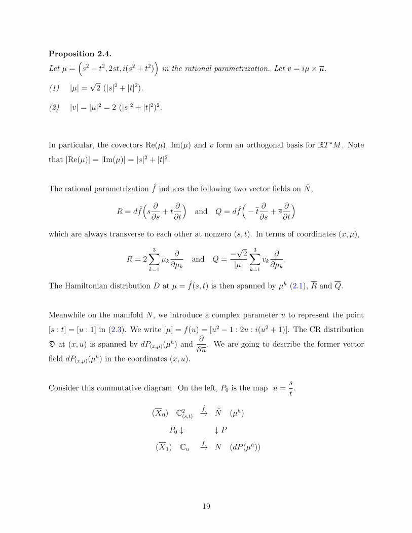
Proposition 2.4.
Let µ =(s2 − t2, 2st, i(s2 + t2)
)in the rational parametrization. Let v = iµ× µ.
(1) |µ| =√
2 (|s|2 + |t|2).
(2) |v| = |µ|2 = 2 (|s|2 + |t|2)2.
In particular, the covectors Re(µ), Im(µ) and v form an orthogonal basis for RT ∗M . Note
that |Re(µ)| = |Im(µ)| = |s|2 + |t|2.
The rational parametrization f induces the following two vector fields on N ,
R = df(s∂
∂s+ t
∂
∂t
)and Q = df
(− t ∂
∂s+ s
∂
∂t
)which are always transverse to each other at nonzero (s, t). In terms of coordinates (x, µ),
R = 23∑
k=1
µk∂
∂µkand Q =
−√
2
|µ|
3∑k=1
vk∂
∂µk.
The Hamiltonian distribution D at µ = f(s, t) is then spanned by µh (2.1), R and Q.
Meanwhile on the manifold N , we introduce a complex parameter u to represent the point
[s : t] = [u : 1] in (2.3). We write [µ] = f(u) = [u2 − 1 : 2u : i(u2 + 1)]. The CR distribution
D at (x, u) is spanned by dP(x,µ)(µh) and
∂
∂u. We are going to describe the former vector
field dP(x,µ)(µh) in the coordinates (x, u).
Consider this commutative diagram. On the left, P0 is the map u =s
t.
(X0) C2(s,t)
f−→ N (µh)
P0 ↓ ↓ P
(X1) Cuf−→ N (dP (µh))
19
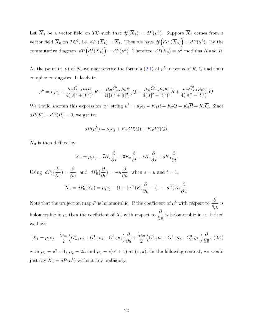
Let X1 be a vector field on TC such that df(X1) = dP (µh). Suppose X1 comes from a
vector field X0 on TC2, i.e. dP0(X0) = X1. Then we have df(dP0(X0)
)= dP (µh). By the
commutative diagram, dP(df(X0)
)= dP (µh). Therefore, df(X0) ≡ µh modulus R and R.
At the point (x, µ) of N , we may rewrite the formula (2.1) of µh in terms of R, Q and their
complex conjugates. It leads to
µh = µjej −µmG
lmkµkµl
4(|s|2 + |t|2)2R +
µmGlmkµkvl
4(|s|2 + |t|2)3Q− µmG
lmkµkµl
4(|s|2 + |t|2)2R +
µmGlmkµkvl
4(|s|2 + |t|2)3Q.
We would shorten this expression by letting µh = µjej −K1R +K2Q−K3R +K4Q. Since
dP (R) = dP (R) = 0, we get to
dP (µh) = µjej +K2dP (Q) +K4dP (Q).
X0 is then defined by
X0 = µjej − tK2∂
∂s+ sK2
∂
∂t− tK4
∂
∂s+ sK4
∂
∂t.
Using dP0
( ∂∂s
)=
∂
∂uand dP0
( ∂∂t
)= −u ∂
∂uwhen s = u and t = 1,
X1 = dP0(X0) = µjej − (1 + |u|2)K2∂
∂u− (1 + |u|2)K4
∂
∂u.
Note that the projection map P is holomorphic. If the coefficient of µh with respect to∂
∂µlis
holomorphic in µ, then the coefficient of X1 with respect to∂
∂uis holomorphic in u. Indeed
we have
X1 = µjej−iµm
2
(G2m1µ3 +G1
m3µ2 +G3m2µ1
) ∂∂u
+iµm
2
(G2m1µ3 +G1
m3µ2 +G3m2µ1
) ∂∂u. (2.4)
with µ1 = u2 − 1, µ2 = 2u and µ3 = i(u2 + 1) at (x, u). In the following context, we would
just say X1 = dP (µh) without any ambiguity.
20

2.3 THE LEVI FORM OF (N ,D) AND (N,D)
A pseudo-hermitian structure of the CR structure D is given by
α =v
|v|=vk|v|ek.
By the identity dei = ωij ∧ ej for every i, its exterior derivative is
dα = D( vk|v|
)∧ ek =
(d( vk|v|
)+vj|v|ωjk
)∧ ek.
Let L be the Levi form of D associated with α, so L = −i dα. We may show that L is a
degenerate bilinear form.
Recall that vk = i(µ × µ)k for every k. We define the horizontal vector field vh at a point
(x, µ) of N , just as the way µh being defined. Explicitly,
vh = vj ej − vmGlmk µk
∂
∂µl− vmGl
mk µk∂
∂µl. (2.5)
Important properties of the differential dvk are listed as follows.
Proposition 2.5. For every j = 1, 2, 3,
(1) dvj(µl
∂
∂µl
)= vj,
(2) dvj(µl
∂
∂µl
)= 0,
(3) dvj(µh) = µmG
kmj vk,
(4) dvj(vh) = vmG
kmj vk.
Proof. Let εjkl be the sign of the permutation (j, k, l), where j, k, l = 1, 2, 3. We say εjkl = 0
when (j, k, l) is not any permutation of numbers 1, 2 and 3. For example ε123 = 1 and
ε213 = −1. We may then write vj = i(εjkl µk µl
)and so
dvj = i εjkl(µl dµk + µk dµl
).
21
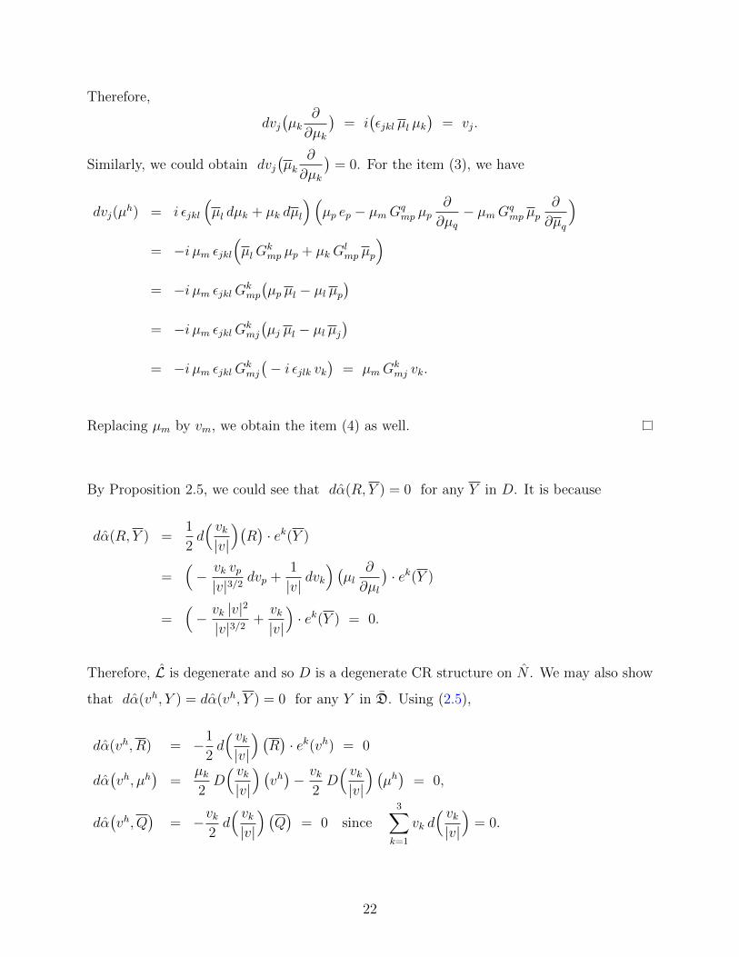
Therefore,
dvj(µk
∂
∂µk
)= i
(εjkl µl µk
)= vj.
Similarly, we could obtain dvj(µk
∂
∂µk
)= 0. For the item (3), we have
dvj(µh) = i εjkl
(µl dµk + µk dµl
)(µp ep − µmGq
mp µp∂
∂µq− µmGq
mp µp∂
∂µq
)= −i µm εjkl
(µlG
kmp µp + µkG
lmp µp
)= −i µm εjklGk
mp
(µp µl − µl µp
)= −i µm εjklGk
mj
(µj µl − µl µj
)= −i µm εjklGk
mj
(− i εjlk vk
)= µmG
kmj vk.
Replacing µm by vm, we obtain the item (4) as well.
By Proposition 2.5, we could see that dα(R, Y ) = 0 for any Y in D. It is because
dα(R, Y ) =1
2d( vk|v|
)(R)· ek(Y )
=(− vk vp|v|3/2
dvp +1
|v|dvk
) (µl
∂
∂µl
)· ek(Y )
=(− vk |v|2
|v|3/2+vk|v|
)· ek(Y ) = 0.
Therefore, L is degenerate and so D is a degenerate CR structure on N . We may also show
that dα(vh, Y ) = dα(vh, Y ) = 0 for any Y in D. Using (2.5),
dα(vh, R) = −1
2d( vk|v|
) (R)· ek(vh) = 0
dα(vh, µh
)=
µk2D( vk|v|
) (vh)− vk
2D( vk|v|
) (µh)
= 0,
dα(vh, Q
)= −vk
2d( vk|v|
) (Q)
= 0 since3∑
k=1
vk d( vk|v|
)= 0.
22
Since both α and vh are real-valued, we could consider the complex conjugation of the above
formulas. As a result, ιvhdα = 0. Moreover, we have the fact that α(vh) = 1.
On the other hand, a pseudo-hermitian structure of the CR manifold (N,D) is given by
α =u+ u
1 + |u|2e1 +
1− |u|2
1 + |u|2e2 +
i(u− u)
1 + |u|2e3 (2.6)
in (x, u). Note that P ∗α = α. Its exterior derivative dα is given by
dα =1
(1 + |u|2)2
(1− u2) du ∧ e1 + (1− u2) du ∧ e1 − 2u du ∧ e2
−2u du ∧ e2 + i(1 + u2) du ∧ e3 − i(1 + u2) du ∧ e3
+
1
1 + |u|2(
(u+ u) de1 + (1− |u|2) de2 + i(u− u) de3).
The associated Levi form LN : D×D→ C is non-degenerate, for
LN( ∂∂u,X1
)= − idα
( ∂∂u,X1
)=
i
2(1 + |u|2)2· 2(1 + |u|2)2 = i
at every (x, u) in N . Here X1 follows from the equation (2.4)
Proposition 2.6. [9] The CR structure (N,D) is non-degenerate and anticlastic.
α is then a contact form of the Levi distribution D⊕D. Indeed, we have
α ∧ (dα)2 =−4i
(1 + |u|2)2du ∧ du ∧ e1 ∧ e2 ∧ e3.
The Reeb vector field T associated with α is given by
T = dP( vh|v|
)=
vj|v|
ej −1
2
vm|v|
(Glmk µk
vl|v|
) ∂
∂u− 1
2
vm|v|
(Glmk µk
vl|v|
) ∂
∂u(2.7)
at any point (x, u). For any Y = dP (Y 0) in D with Y 0 in D,
dα(T, Y ) = P ∗dα( vh|v|, Y 0
)= dα
( vh|v|, Y 0
)= 0.
23
2.4 CR STRUCTURE ON THE SPHERE BUNDLE OF M
The twistor CR manifold N of (M, g) is diffeomorphic to the sphere bundle (S) of M . We
may construct a CR structure Π on S such that D is CR equivalent to Π. This process will
make use of the horizontal and vertical spaces of the tangent bundle of M [16].
Corresponding to the orthonormal framee1, e2, e3
, a unit tangent vector λ = λiei at x ∈M
is represented by (x, λ) =(x1, x2, x3, λ1, λ2, λ3
)with
∑3i=1 λ
2i = 1. Let X = ξiei be a tangent
vector on TxM . The horizontal lift of X at (x, λ) on TS is
Xh = ξi ei − ξj Gljk λk
∂
∂λl, (2.8)
The horizontal bundle H of S is defined by
H(x,λ) =Xh ∈ T(x,λ)S | g(X,λ) = 0
at every point (x, λ). On the other hand, the vertical lift of X at (x, λ) is
Xv = ξi∂
∂λi. (2.9)
We define the vertical bundle V of S by
V(x,λ) =Xv ∈ T(x,λ)S | g(X,λ) = 0
.
at every point (x, λ) on S.
An almost complex structure J is defined on the 4-dimensional distribution V ⊕ H. Given
λ = λiei and η = ηiei on TxM , the cross product λ× w is given by
λ× η =(λ2η3 − λ3η2
)e1 +
(λ3η1 − λ1η3
)e2 +
(λ1η2 − λ2η1
)e3.
At the point (x, λ), for every Xh ∈ H and Xv ∈ V , we let
JXh = (λ×X)h and JXv = (λ×X)v.
24

Explicitly, if X is on TxM with g(X,λ) = 0, then by (2.8) and (2.9)
JXh = (λ×X)i ei − (λ×X)j Gljk λk
∂
∂λland JXv = (λ×X)i
∂
∂λi
at (x, λ).
Let Π be the antiholomorphic bundle over S corresponding to V ⊕H and J . At every (x, λ),
the complex 2-plane Π is spanned by the vectors in the form of Xh + iJXh and Xv + iJXv,
given that g(X,λ) = 0.
Π is integrable and therefore Π defines a CR structure on the sphere bundle S.
This CR manifold (S,Π) can be identified with the twistor CR manifold (N,D) of M . The
identification Φ : N → S is defined as follows. At any point x ∈ M , Φ maps from the fibre
Nx to the fibre Sx such that
Φ([µ]) =v
|v|=iµ× µ|µ|2
,
where µ is any representative in the equivalence class [µ]. In terms of (x, u), we have
Φ(u) =u+ u
1 + |u|2e1 +
1− |u|2
1 + |u|2e2 +
i(u− u)
1 + |u|2e3. (2.10)
We also let the composite function Φ : N → S be defined by Φ = Φ P .
Proposition 2.7. [9] Φ : N → S is a CR isomorphism between D and Π.
Proof. The differential map dΦ at (x, u) is described as follows. First of all, we have
dΦ( ∂∂u
)= d
( vk|v|)( ∂∂u
) ∂
∂λk
=1
(1 + |u|2)2
((1− u2)
∂
∂λ1
− 2u∂
∂λ2
+ i(1 + u2)∂
∂λ3
)=
−1
(1 + |u|2)2
(µl
∂
∂λl
).
25
By taking the complex conjugate, we have dΦ( ∂∂u
)=
−1
(1 + |u|2)2· µl
∂
∂λl. Moreover,
dΦ(X1
)= dΦ
(µh)
= µjej + d( vk|v|)(µh) ∂
∂λk
= µjej +( 1
|v|dvk −
vk|v|3
vjdvj
)(µh) ∂
∂λk
= µjej +1
|v|µmG
lmkvl
∂
∂λk− vk|v|3
vj · µmGlmjvl
∂
∂λk
= µjej − µmGkml
vl|v|
∂
∂λk.
Therefore, dΦ(x,u) sends D(x,u) isomorphically to Π(x,Φ(u)).
2.5 EMBEDDING INTO COMPLEX 3-MANIFOLD
If M is a real analytic 3-manifold, then D is a real analytic CR structure on N . By
Theorem 1.1, N is locally embeddable to C3 and it could be globally embedded to a complex
3-manifold. LeBrun showed that the converse also holds in [9].
Theorem 2.8. [9] Let M be a smooth 3-manifold equipped with the conformal structure [g].
Let N be the twistor CR manifold of M equipped with the CR structure D. Then, (N,D) is
embeddable into a complex 3-manifold if and only if M admits a real analytic atlas on which
there is a real analytic metric g in class [g].
When M is equipped with a flat metric, and (x, u) are coordinates on N , D is spanned by
X1 = (u2 − 1)∂
∂x1
+ 2u∂
∂x2
+ i(u2 + 1)∂
∂x3
and X2 =∂
∂u.
Let f : N → C be a CR function on N . Then we must have fu = 0 and
(u2 − 1)fx1 + 2u fx2 + i(u2 + 1)fx3 = 0 (2.11)
26

We may first let γ(t) =(x1(t), x2(t), x3(t), u(t)
)be a characteristic curve of (2.11), i.e.
x′1 = u2 − 1, x′2 = 2u, x′3 = i(u2 + 1) and u′ = 0.
Immediately we have u = u0 for some constant u0, and so x′1 = u20 − 1.
dx2
dx1
=x′2(t)
x′1(t)=
2u
u2 − 1=⇒ x2 =
2ux1
u2 − 1+ c0
for some constant c0. It could be written as (u2 − 1)x2 − 2ux1 = c0(u20 − 1). Similarly,
dx3
dx1
=x′3(t)
x′1(t)=i(u2 + 1)
u2 − 1=⇒ x3 =
i(u2 + 1)x1
(u2 − 1)+ c1
for some constant c1. Therefore, (u2 − 1)x3 − i(u2 + 1)x1 = (u20 − 1)c1.
Hence, the solution f to equation (2.11) is a function of
u, 2ux1 − (u2 − 1)x2 and i(u2 + 1)x1 − (u2 − 1)x3.
We make use of these three basic solutions and letw1 = u,
w2 = 2ux1 − (u2 − 1)x2,
w3 = i(u2 + 1)x1 − (u2 − 1)x3.
In order to obtain an algebraic relation between w1, w2 and w3, we note that
(u2 − 1)w3 − (u2 − 1)w3 = 2i x1
(|u|4 − 1
),
(u2 − 1)w2 − (u2 − 1)w2 = 2x1(u− u)(1 + |u|2).
This implies
(w21 − 1)w3 − (w2
1 − 1)w3
2i(|w1|4 − 1)= x1 =
(w21 − 1)w2 − (w2
1 − 1)w2
2(w1 − w)(1 + |w1|2).
As a result, (w1, w2, w3) satisfies the relation
(|w1|2 − 1)(
(w21 − 1)w2 − (w2
1 − 1)w2
)= i(w1 − w1)
((w2
1 − 1)w3 − (w21 − 1)w3
).
27

We could then simplify the relation by setting
y1 = w1 = u,
y2 =−w2 − i w1w3
w21 − 1
= ux1 + x2 + i u x3,
y3 =w3 − i w1w2
w21 − 1
= −i x1 + i u x2 − x3.
The relation between y1, y2 and y3 defines a hyperquadric Q in C3,
Q =(y1, y2, y3
)| y2 − y2 = −i
(y1 y3 + y3 y1
).
Let [ξ] = [ξ0 : ξ1 : ξ2 : ξ3] be the homogeneous coordinates on CP 3. C3 is embedded to CP 3
in the way that (y1, y2, y3) is mapped to [1 : y1 : y2 : y3]. That means, yj = ξj/ξ0 for ξ0 6= 0.
Then, Q is embedded to a hyperquadric Q′ (in CP 3),
Q′ =[ξ0 : ξ1 : ξ2 : ξ3
]| ξ2 ξ0 − ξ2 ξ0 = −i
(ξ1 ξ3 + ξ1 ξ3
).
Let N0 be the coordinate chart of (x, u) on N . We may identify N0 with Q, and map the
CR manifold N to an open subset of Q′.
Proposition 2.9. Let φ(x, u) = (y1, y2, y3) be defined as above.
(1) φ defines a CR isomorphism from N0 to Q.
(2) φ could be extended to a CR isomorphism Φ from N to an open subset of Q′,
U ′ = Q′ ∩
[ξ] ∈ CP 3 | ξ0 6= 0 or ξ1 6= 0
.
28

3.0 CR STRUCTURE BY AFFINE CONNECTIONS
Fix N to be the twistor CR manifold of (M, [g]). In Chapter 2, we mentioned that the CR
structure D depends on the conformal class of g only. It means that we may replace the
Riemannian connection of g by that of e2λg to obtain the same CR structure. This idea
would be generalized to any Weyl connection of g.
Moreover, we may consider any metric connections with nonzero torsion on M . If M is
embedded to a 4-manifold, then we could define such a connection by the second fundamental
form of M . In this case, we could get to different CR structures than D on N .
3.1 WEYL CONNECTION ON (M, g)
Definition. [1] Suppose [g] is a conformal structure on M . A Weyl structure on a manifold
M is a map F : [g] → Ω1(M), satisfying the condition F (eλg) = F (g) − dλ for all λ in
C∞(M).
Given a metric g and a 1-form α on M , a Weyl structure is determined by the equations
F (g) = −α and F (eλg) = −α − dλ. For this Weyl structure, there is a unique torsion-free
affine connection ∇ on M , characterized by (1) ∇g = α⊗ g and (2) ∇ is torsion free. It is
called the Weyl connection of the Weyl structure determined by g and α.
29
Lete1, e2, e3
be an orthonormal frame on (M, g). Write α = αke
k. The Christoffel symbols
of the Weyl connection ∇ on M are given by Gkij = g(∇eiej, ek).
To distinguish ∇ from the Riemannian connection of (M, g), we denote the later by ∇ and
write Gkij = g(∇eiej, ek). The relation between ∇ and ∇ is given by the identity,
∇eiej = ∇eiej − Skijek.
Here Skij =1
2
(αiδjk + αjδik − αkδij
). In terms of the Christoffel symbols of ∇ and ∇,
Gkij = Gkij − Skij.
Suppose X = ξiei is a tangent vector on TxM . Let (x, λ) be a point on N , regarded as the
sphere bundle of M here, with λ = λiei being a unit vector on TxM . Assume g(X,λ) = 0.
Similar to (2.8), the horizontal lift of X by ∇ at (x, λ) is
XH = ξj ej − ξj Gljk λk∂
∂λl
= ξj ej − ξj Gljk λk
∂
∂λl+ ξj S ljk λk
∂
∂λl
= Xh + ξj
(1
2(αj δkl + αk δjl − αl δjk)
)λk
∂
∂λl
= Xh +1
2α(X)λv +
1
2α(λ)Xv.
Here Xh is the horizontal lift of X by ∇ at (x, λ). Since λv is in the radial direction to the
sphere bundle, we omit this term and define the horizontal lift of X at (x, λ) by
XH = Xh +1
2α(λ)Xv. (3.1)
The horizontal bundle H(x,λ) is then the space of all horizontal vectors XH at (x, λ) with
g(X,λ) = 0. The vertical lift of X at (x, λ) is again defined by (2.9),
Xv = ξj∂
∂λj,
30
and the vertical bundle V(x,λ) consists of vertical vectors Xv at (x, λ) given g(X,λ) = 0.
Note that the rank-4 bundle V ⊕H is exactly the one we get from ∇. We define an almost
complex structure J on V ⊕H by
JXH = (λ×X)H and JXv = (λ×X)v
at (x, λ). The almost complex structure J on V ⊕ H is the same almost complex structure
we define in Section 2.4 on V ⊕H, for
JXh = J(XH − 1
2α(λ)Xv
)= (λ×X)h +
1
2α(λ)(λ×X)v − 1
2α(λ)(λ×X)v
= (λ×X)h.
Therefore, by any Weyl connection ∇ on M with respect to g and α, we define the same CR
structure D on N .
Proposition 3.1. Let g be a metric and α be a 1-form on the 3-manifold M . Let ∇ be
the Weyl connection on M determined by g and α. Then, the CR structure defined on the
5-manifold N by ∇ coincides with D.
As a remark, α could be a complex 1-form on M , and we define the horizontal lift of vector
X at (x, λ) by (3.1). The almost complex structure is also defined by JXH = (λ×X)H and
JXv = (λ × X)v. We may see that the linear span of XH and Xv with g(X,λ) = 0 is a
subspace of the complexified V ⊕ H. The corresponding antiholomorphic bundle coincides
with D.
Therefore, we get to the same CR structure D on N when α is complex-valued.
31
3.2 METRIC CONNECTION WITH TORSION
The description of the torsion tensor in this section is quoted from [17], where readers may
find out more details and applications of the torsion tensor.
Let ∇ be a metric connection with nonzero torsion tensor on the 3-manifold (M, g). For
any vector field X and Y on M , we have T (X, Y ) = ∇XY − ∇YX − [X, Y ]. Given an
orthonormal framee1, e2, e3
on M , we let T kij’s be the coefficients of T , i.e.
T (ei, ej) = T kijek.
We denote the Riemannian connection of g by ∇ and its Christoffel symbols by Gkij as in
Section 3.1. The Christoffel symbols of ∇ are defined by Gkij = g(∇eiej, ek
)with
Gkij = Gkij +
1
2
(T kij − T
jik − T
ijk
). (3.2)
The torsion tensor T can be decomposed to three components in a sum,
T kij =1
2
(Tiδkj − Tjδki
)+τ
6εijk + qijk. (3.3)
The terms Ti, τ and qijk are defined in the below context. The term εijk is the same as in
Proposition 2.5. We would introduce these three components of (3.3) separately.
(I) The trace component of T :1
2
(Tiδkj − Tjδki
)Let Ti =
3∑k=1
T kik be the trace of T acting on ei. If we write P kij =
1
2
(Tiδkj − Tjδki
), then
we have Pijk = −Pjik and Pijk + Pjki + Pkij = 0 for every i, j, k.
(II) The scalar function τ on M :τ
6εijk
We may say that εijk = 6 e1 ∧ e2 ∧ e3. So ε123 = 1, ε213 = −1 and so on. We define
τ =3∑
i,j,k=1
εijk · T kij
τ is independent of the choice of the positively oriented orthonormal frame.
32

(III) The trace-free cocyclic component of T : qijk
The term qijk is defined by the difference,
qijk = T kij −1
2
(Ti δkj − Tj δki
)− τ
6εijk.
We have the following properties about qijk’s.
Proposition 3.2.
(1) qijk = −qjik
(2)3∑j=1
qijj = 0
(3)3∑
i,j,k=1
εijk qijk = 0
The item (2) comes from the contraction of the torsion tensor T .
3∑j=1
qijj =3∑j=1
T jij −1
2
3∑j=1
(Ti − Tj δji
)= Ti −
1
2
(3Ti − Ti
)= 0
For the item (3), we multiply εijk by qijk and obtain∑i,j,k
εijk qijk = τ −(∑i,j,k
εijk Pijk
)− τ
6
∑i,j,k
ε2ijk = τ − 0− τ = 0.
Let q be a (1, 1)-tensor on M using the coefficients qijk’s. Namely,
q(ek) = qlkel and qijk =3∑l=1
εijl qlk.
The second identity means that qlk =1
2
3∑i,j=1
εijl qijk. Note tr(q) = qkk = 0. When k 6= l,
qlk =1
2
∑i,j
εijl qijk = qmkk = −qmll = qkl
for (k, l,m) being a positive permutation within 1, 2, 3. So qlk = qkl for every k, l.
33

We then turn to the horizontal lift of vector fields from M to N by ∇. Let (x, λ) be a point
on N which represents the unit vector λiei at x. Let X = ξiei be a vector on TxM orthogonal
to λ. By (3.2), the horizontal lift of X at (x, λ) by ∇ is given as
XH = Xh − 1
2ξj(T ljk − T kjl − T
jkl
)λk
∂
∂λl. (3.4)
We would then examine the effect of each linear component in (3.4) to XH . To begin with,
we set T kij =1
2
(Ti δkj − Tj δki
), τ = 0 and qijk = 0. That is,
T ljk − T kjl − Tjkl = −Tk δjl + Tl δjk.
It leads to
XH = Xh − 1
2ξj
(− Tk δjl + Tl δjk
)λk
∂
∂λl
= Xh +1
2(Tkλk) ξl
∂
∂λl− 1
2(ξjλj)Tl
∂
∂λl
= Xh +1
2(trT)(λ)Xv.
Next, we set T kij =τ
6εijk with τ 6= 0.
T ljk − T kjl − Tjkl =
τ
6
(εjkl − εjlk − εklj
)=
τ
6εjkl
It implies that
XH = Xh − 1
2ξj
(τ6εjkl
)λk
∂
∂λl
= Xh − τ
12
(ξj εjkl λk
) ∂
∂λl
= Xh +τ
12
(λ×X
)v.
Both the first and second components of T would result in the same CR structure D on N ,
under the construction from (3.4). We skip the details here.
34
For the third component, we set T kij = qijk = εijl qlk. From Proposition 3.2, we have
T ljk − T kjl − Tjkl = qjkl − qjlk − qklj = − 2 qklj.
By (3.4), we have
XH = Xh −(λ× q(X)
)v= Xh − λk εkml
(qmj ξj
) ∂∂λl
. (3.5)
The almost complex structure J on the horizontal and vertical bundles is given by
JXH = (λ×X)H = (λ×X)h −(λ× q(λ×X)
)vand JXv = (λ×X)v. (3.6)
at (x, λ) with X ⊥ λ. Let D(q) be the antiholomorphic bundle regarding (3.5) and (3.6). In
general, D(q) is different from D.
Proposition 3.3. The complex distribution D(q) is a CR structure on N .
The vector field XH (3.5) is pulled back to the local chart of (x, u) on N . Let Φ be the
identification map in (2.10) from N to the sphere bundle S. When λ = Φ(u), we get
λ1 =u+ u
1 + |u|2, λ2 =
1− |u|2
1 + |u|2and λ3 =
i(u− u)
1 + |u|2.
Recall that [µ] = f([u : 1]) in (2.3), and we have µ =(u2 − 1, 2u, i(u2 + 1)
). We know that
dΦ( ∂∂u
)=
−1
(1 + |u|2)2
(µl
∂
∂λl
)and dΦ
(X1
)= µjej − µmGk
mlλl∂
∂λk,
where X1 is the vector in D from (2.4). From (3.5) and (3.6), the complex distribution D(q)
at (x, λ) is spanned by the vectors Y 1 and Y 2.
Y 1 = µjej − µmGlmkλk
∂
∂λl− λk εkml
(qmj µj
) ∂∂λl
Y 2 = µl∂
∂λl
Note that dΦ(− (1 + |u|2)2 ∂
∂u
)= Y 2.
35

Let Y 0 be the third component of Y2. That is,
Y 0 = −λk εkml(qmj µj
) ∂
∂λl
= −µj[(λ2 q
j3 − λ3 q
j2
) ∂
∂λ1
+(λ3 q
j1 − λ1 q
j3
) ∂
∂λ2
+(λ1 q
j2 − λ2 q
j1
) ∂
∂λ3
].
Let Y 0 = c1 µl∂
∂λl+ c2 , µl
∂
∂λl. So we have,
Y 0 ·(µl
∂
∂λl
)= c2|µ|2 = 2(1 + |u|2)2c2
under the Sasaki metric on TM .
c2 =−µj
2(1 + |u|2)2
[(λ2 q
j3 − λ3 q
j2
)µ1 +
(λ3 q
j1 − λ1 q
j3
)µ2 +
(λ1 q
j2 − λ2 q
j1
)µ3
]=
1
2(1 + |u|2)2
[q1
1
(− µ1 µ2 λ3 + µ1 µ3 λ2
)+ q2
2
(µ1 µ2 λ3 − µ2 µ3 λ1
)+ q3
3
(− µ1 µ3 λ2 + µ2 µ3 λ1
)+ q2
1
(µ2
1 λ3 − µ22 λ3 − µ1 µ3 λ1 + µ2 µ3 λ2
)+ q3
1
(− µ2
1 λ2 + µ23 λ2 − µ2 µ3 λ3 + µ1 µ2 λ1
)+ q3
2
(µ2
2 λ1 − µ23 λ1 + µ1 µ3 λ3 − µ1 µ2 λ2
)].
By the fact that λ× µ = −i µ, λ× µ = i µ, we may simplify c2 to get
c2 =1
2(1 + |u|2)2
[i (µ2
3 − µ21) q1
1 + i (µ23 − µ2
2) q22 − 2 i µ1 µ2 q
21 − 2 i µ1 µ3 q
31 − 2 i µ2 µ3 q
32
].
Therefore,
dΦ−1(Y 1) = dΦ−1(µjej − µmGl
mkλk∂
∂λl
)+ dΦ−1(Y 0)
= X1 + dΦ−1(c1µl
∂
∂λl+ c2µl
∂
∂λl
)= X1 − c1(1 + |u|2)2 ∂
∂u− c2(1 + |u|2)2 ∂
∂u
36

dΦ−1(Y 1) = µj ej −i
2µm
(G2m1 µ3 +G1
m3 µ2 +G3m2 µ1
) ∂
∂u
+[ i
2(µ2
1 − µ23) q1
1 +i
2(µ2
2 − µ23) q2
2 + i µ1 µ2 q21 + i µ1 µ3 q
31 + µ2 µ3 q
32
] ∂
∂u
− c1 (1 + |u|2)2 ∂
∂u.
As a result, the CR structure D(q) at the point (x, u), is spanned by X2 =∂
∂uand
X1 = µj ej −i
2µm
(G2m1 µ3 +G1
m3 µ2 +G3m2 µ1
) ∂
∂u+ uT ·C · q ∂
∂u. (3.7)
Here we define
uT ·C · q = ( 1 u u2 u3 u4 )
i 0 1 i2
0
0 −2i 0 0 −2
0 0 0 3i 0
0 2i 0 0 −2
i 0 −1 i2
0
q11
q21
q31
q22
q32
correspondingly.
In general, for every trace-free and symmetric (1,1)-tensor q on M , we may define a
corresponding CR structure D(q) on N by (3.7). We would say that q is the trace-free
torsion tensor on M . The complex function w = uT ·C ·q is holomorphic in u, and we would
call it by the torsion function of D(q) in the following context.
37

3.3 THE TRACE-FREE SECOND FUNDAMENTAL FORM
When M is embedded to a 4-manifold M , the trace-free second fundamental form of M
would become the trace-free torsion tensor q. Suppose g is the metric on M and ∇ is its
Levi-Civita connection. Lete1, e2, e3
be an orthonormal frame on M and let n be the unit
normal vector to M . The second fundamental form on M is then defined by
II(u, v) = −g(∇un, v
)for u, v on TM.
Following from LeBrun’s paper [10], we would define a metric connection with torsion (∇′ )
on M by letting ∇′uv = ∇uv −(v × ∇un
)for any u, v on TM . Through our discussion in
Section 3.2, the trace-free torsion tensor q is given by
q(u) = − ∇un−1
3tr(II) · Id for u ∈ TM. (3.8)
When M is a Riemannian manifold, we let
∇eiej = Gkij ek + G0ij n, ∇ein = Gki0 ek and ∇nej = Gk0j ek + G0
0j n. (3.9)
We have the symmetries Gkij = −Gjik and G0ij = G0
ji = −Gji0. Note that Gkij’s are also the
Christoffel symbols of the Riemannian connection on M . We then get to II(em, en) = G0mn
and tr(II) =∑3
k=1 G0kk. The components of q could be found by
qlk = G0kl −
1
3
( 3∑m=1
G0mm
)δkl.
Putting q to (3.7), the torsion function w = uT ·C · q becomes
w =( i
2G0
11 −i
2G0
33 + G013
)−(2iG0
12 + 2G023
)u+
(2iG0
22 − iG011 − iG0
33
)u2
+(2iG0
12 − 2G023
)u3 +
( i2G0
11 −i
2G0
33 − G013
)u4.
(3.10)
The same definition of q in (3.8) by the trace-free second fundamental form could also be
carried out naturally when M is Lorentzian. The torsion function w obtained would then
be identical to (3.10) but with a minus sign to every G0ij on the right.
38

When M is a Lorentzian 4-manifold and M is a space-like submanifold of M , we could also
define a corresponding CR structure D(q) on M by the trace-free second fundamental form
but in an alternative way. It results in using i times q (3.8) to construct the CR structure
by (3.7) on the twistor CR manifold N of M .
We keep the orthonormal frame of n, e1, e2 and e3 on M but with g(n,n) = −1. Following
the definition in (3.9), we have II(em, en) = −Gnm0 = −G0mn and tr(II) = −
∑3k=1 G0
kk. Since
g is a Lorentzian metric, the null cones on M form a 6-dimensional manifold
N =
(x, v) ∈ TM | x ∈M, v ∈ TxM, g(v, v) = 0 with v 6= 0.
The parallel transport of null vectors along tangential vectors on M , would define a CR
structure on the sphere bundle S of M .
For a point (x, v) on N , we let v = v0 n +∑3
j=1 vjej. Let u = ujej be a tangent vector on
TxM . The horizontal lift of u by ∇ at (x, v) is
uH = ui ei − uj Gljk vk∂
∂vl− uj Glj0 v0
∂
∂vl− uj G0
jk vk∂
∂v0
.
uH is a vector on TN since
(− v0 dv0 + vi dvi
)(uH) = uj G0
jk vk v0 − uj Gijk vk vi − uj Gij0 v0 vi = 0.
Suppose (x, λ) are the coordinates on S corresponding toe1, e2, e3
. We would define a
projection map Φ from N to S, Φ(v) =(vjv0
)ej. Through the differential map dΦ at (x, v),
dΦ(uH) = uj ej − uj Gljk λk∂
∂λl− uj Glj0
∂
∂λl+ uj Gkj0 λk λl
∂
∂λl(3.11)
at λ = Φ(v). From here we denote dΦ(uH) by uH directly. (3.11) is equivalent to
uH = uh −(∇un− g(∇un, λ)λ
)v. (3.12)
Here uh is the horizontal lift of u at (x, λ) by the Riemannian connection on M , defined by
the first two terms of (3.11).
39

The vertical lift of u at (x, λ) remains as uv = uj∂∂λj
. The horizontal and vertical bundles
of S at (x, λ) consist of all horizontal and vertical lifts of tangent vectors u at x respectively,
given that g(u, λ) = 0. The almost complex structure J on TS is defined by JuH = (λ×u)H
and Juv = (λ× u)v.
Therefore, the corresponding antiholomorphic bundle D defines a CR structure on S. By
Proposition 2.7, it is equivalent to say that D is on the twistor CR manifold N of (M, g).
Proposition 3.4. D coincides with the CR structure D(q) on N , where the trace-free torsion
tensor q is defined by the trace-free second fundamental form of M multiplied by i, i.e.,
q = − i ∇n− i
3tr(II) · Id.
Proof. By (3.6), the CR distribution D(q) at (x, λ) is spanned by
uH + i(λ× u)H = uh + i(λ× u)h −(λ× q(u)
)v − i(λ× q(λ× u))v
and uv + i(λ× u)v given that g(u, λ) = 0. Put q(u) = −i ∇un−i
3tr(II)u. First of all we
assume that u is a unit vector orthogonal to λ. So we get
tr(II) = − g(∇un, u)− g(∇λ×un, λ× u)− g(∇λn, λ).
We compute for
λ× q(u) = λ×(− i ∇un−
i
3tr(II)u
)= −i
(g(∇un, u
)λ× u− g
(∇un, λ× u
)u)− i
3tr(II)λ× u
= i g(∇λ×un, u
)u− i g
(∇un, u
)λ× u− i
3tr(II)λ× u
= i g(∇λ×un, u
)u+ i g
(∇λ×un, λ× u
)λ× u
+i g(∇λn, λ
)λ× u+ i tr(II)λ× u− i
3tr(II)λ× u.
= i(∇λ×un− g
(∇λ×un, λ
)λ)
+ i g(∇λn, λ
)λ× u+
2i
3tr(II)λ× u.
40

Then we compute for
i λ× q(λ× u) = i λ×(− i ∇λ×un−
i
3tr(II)λ× u
)= λ× ∇λ×un−
1
3tr(II)u
= λ×(g(∇λ×un, u
)u+ g
(∇λ×un, λ× u
)λ× u
)− 1
3tr(II)u
= g(∇λ×un, u
)λ× u− g
(∇λ×un, λ× u
)u− 1
3tr(II)u
= g(∇un, λ× u
)λ× u+ g
(∇un, u
)u+ g
(∇λn, λ
)u+
2
3tr(II)u
=(∇un− g
(∇un, λ
)λ)
+ g(∇λn, λ
)u+
2
3tr(II)u.
Therefore,
uH + i (λ× u)H
=(uh + i (λ× u)h
)−[(∇un− g
(∇un, λ
)λ)v
+ i(∇λ×un− g
(∇λ×un, λ
)λ)v]
−g(∇λn, λ
) (uv + i (λ× u)v
)− 2
3tr(II)
(uv + i(λ× u)v
).
The assumption g(u, u) = 1 is redundant since u is linear on every component of the sum
in λ× q(u) and i λ× q(λ× u). Compare the last equation with (3.12), it is clear that D(q)
coincides with D on N .
Proposition 3.4 suggests that the trace-free torsion tensor q could be complex-valued in
general. When we go back to (3.7), we may replace every qlk’s by
qlk = − iG0kl +
i
3
( 3∑m=1
G0mm
)δkl.
Therefore the torsion function w = uT ·C · q is
w =(1
2G0
11 −1
2G0
33 − iG013
)+(− 2G0
12 + 2 iG023
)u+
(2G0
22 − G011 − G0
33
)u2
+(2G0
12 + 2iG023
)u3 +
(1
2G0
11 −1
2G0
33 + iG013
)u4.
(3.13)
41
4.0 FEFFERMAN METRIC (I)
Given a 3-manifold M , we could define CR structures on its twistor CR manifold N by a
trace-free torsion tensor q. In general we may choose a complex-valued function w on N
holomorphic in the vertical parameter to replace uT ·C · q in (3.7). The corresponding CR
structure would be named D(w). In this chapter, we assume that M is equipped with a flat
metric.
4.1 THE LOCAL MODEL OF D(w)
Suppose M is a flat space of coordinates x = (x1, x2, x3) and N is the twistor CR manifold
(sphere bundle) of M . The local model of the CR structure D(w) on N is described by
X1 = (u2 − 1)∂
∂x1
+ 2u∂
∂x2
+ i(u2 + 1)∂
∂x3
+ w(x, u)∂
∂u
X1 = (u2 − 1)∂
∂x1
+ 2u∂
∂x2
− i(u2 + 1)∂
∂x3
+ w(x, u)∂
∂u
X2 =∂
∂u
X2 =∂
∂u
T =u+ u
1 + |u|2∂
∂x1
+1− |u|2
1 + |u|2∂
∂x2
+i(u− u)
1 + |u|2∂
∂x3
(4.1)
at (x, u), where w is an arbitrary complex function holomorphic in u. The contact form of
D(w) is always chosen by (2.6), i.e.
α =u+ u
1 + |u|2dx1 +
1− |u|2
1 + |u|2dx2 +
i(u− u)
1 + |u|2dx3. (4.2)
42

The vector field T in (4.1) is the Reeb vector field of α. Also, we letθ1, θ2, θ1, θ2, α
be the
dual coframe ofX1, X2, X1, X2, T
.
Let L be the Levi form of α, then it components are given by hαβ = L(Xα, Xβ) with
h =
h11 h12
h21 h22
=
0 −i
i 0
(4.3)
In particular, we have h−1 = h and so hαβ = hαβ for α, β = 1, 2. Moreover, the eigenvalues
of h is ±1, so D(w) is anticlastic.
Let g be the Webster metric associated with α, and let ∇ be the Tanaka Webster-connection
of α. Following our notation in Section 1.4, we let
∇XmXn = ΓkmnXk, ∇XmXn = ΓkmnXk and ∇TXn = Γk0nXk
accordingly. The Christoffel symbols Γkmn, Γkmn and Γk0n could be found by (1.1), replacing Tn
by Xn and Tn by Xn. In this process, we will have to compute for the Lie brackets between
X1, X1, X2, X2 and T .
Let µ = µj∂∂xj
and µ = µj∂∂xj
, in which µ1 = u2 − 1, µ2 = 2u and µ3 = i(u2 + 1). We denote
the directional derivative of w along µ (or µ) by Dµw (or Dµw). So,
Dµw = (u2 − 1)wx + 2uwy + i(u2 + 1)wz and Dµw = (u2 − 1)wx + 2uwy − i(u2 + 1)wz.
The vector v|v| in (2.10) coincides with T when M is flat but not in general. We also denote
the directional derivative of w along v|v| by D v
|v|w. Moreover, the symbol DuDµw would mean
the second derivative of w first by µ and then by u. Other symbols of second derivatives are
similarly defined.
43
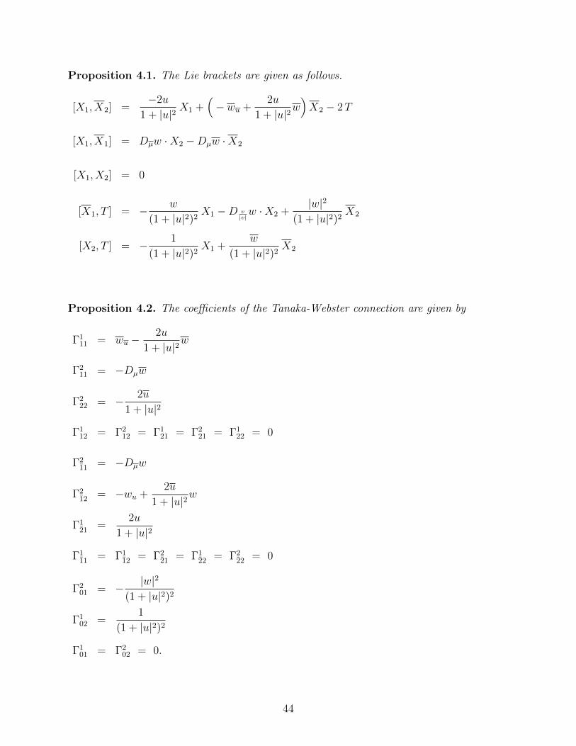
Proposition 4.1. The Lie brackets are given as follows.
[X1, X2] =−2u
1 + |u|2X1 +
(− wu +
2u
1 + |u|2w)X2 − 2T
[X1, X1] = Dµw ·X2 −Dµw ·X2
[X1, X2] = 0
[X1, T ] = − w
(1 + |u|2)2X1 −D v
|v|w ·X2 +
|w|2
(1 + |u|2)2X2
[X2, T ] = − 1
(1 + |u|2)2X1 +
w
(1 + |u|2)2X2
Proposition 4.2. The coefficients of the Tanaka-Webster connection are given by
Γ111 = wu −
2u
1 + |u|2w
Γ211 = −Dµw
Γ222 = − 2u
1 + |u|2
Γ112 = Γ2
12 = Γ121 = Γ2
21 = Γ122 = 0
Γ211 = −Dµw
Γ212 = −wu +
2u
1 + |u|2w
Γ121 =
2u
1 + |u|2
Γ111 = Γ1
12 = Γ221 = Γ1
22 = Γ222 = 0
Γ201 = − |w|2
(1 + |u|2)2
Γ102 =
1
(1 + |u|2)2
Γ101 = Γ2
02 = 0.
44

The curvature tensor of ∇ is denoted by R. According to (1.2), we may find out Rmnkl,
which represents the coefficient of Xn in the vector R(Xk, X l)Xm. The Ricci tensor (ric)
and the scalar curvature (ρ) of ∇ follow from (1.3).
Many of our equations and statements are found and justified by computer programming. In
this simplified model that M is flat, however, we may also justify results by direct argument.
Proposition 4.3. The Ricci tensor of the Tanaka-Webster connection is given by
ric(X1, X1) =4|w|2
(1 + |u|2)2−DuDµw −DuDµw +
4u
1 + |u|2Dµw +
4u
1 + |u|2Dµw,
ric(X1, X2) = −(wuu −
6u
1 + |u|2wu +
12u2
(1 + |u|2)2w),
ric(X2, X1) = −(wuu −
6u
1 + |u|2wu +
12u2
(1 + |u|2)2w),
ric(X2, X2) =4
(1 + |u|2)2.
Proof. The first coefficient is R11 = R11
11 +R12
21. We have
R11
11 = dΓ111(X1)− dΓ1
11(X1)− Γp11Γ11p + Γp
11Γ1
1p + Γp11
Γ1p1 − Γp
11Γ1p1 + 2iΓ1
01h11
= 0− dΓ111(X1)− 0 + 0 + 0− Γ2
11Γ121 + 0
= −(DuDµw −
2u
1 + |u|2Dµw −
2|w|2
(1 + |u|2)2
)+
2u
1 + |u|2Dµw
= −DuDµw +4u
1 + |u|2Dµw +
2|w|2
(1 + |u|2)2,
R12
21 = dΓ211(X2)− dΓ2
21(X1)− Γp21Γ21p + Γp
11Γ2
2p + Γp12
Γ2p1 − Γp
21Γ2p1 + 2iΓ2
01h21
= dΓ211(X2)− 0− 0 + Γ2
11Γ222 + 0− Γ1
21Γ211 − 2Γ2
01
= (−DuDµw) +2u
1 + |u|2Dµw +
2u
1 + |u|2Dµw +
2|w|2
(1 + |u|2)2
= −DuDµw +4u
1 + |u|2Dµw +
2|w|2
(1 + |u|2)2.
45

So R11 is obtained. Next we consider R12 = R11
12 +R12
22.
R11
12 = dΓ121(X1)− dΓ1
11(X2)− Γp11Γ12p + Γp
21Γ1
1p + Γp21
Γ1p1 − Γp
12Γ1p1 + 2iΓ1
01h12
= d( 2u
1 + |u|2)
(X1)− d(wu −
2u
1 + |u|2w)
(X2) + Γ121Γ1
11 − Γ212Γ1
21
= − 2u2
(1 + |u|2)2w −
(wuu −
2u
1 + |u|2wu +
2u2
(1 + |u|2)2w)
+2u
1 + |u|2(wu −
2u
1 + |u|2w)− 2u
1 + |u|2(− wu +
2u
1 + |u|2w)
= −wuu +6u
1 + |u|2wu −
12u2
(1 + |u|2)2w
R12
22 = dΓ221(X2)− dΓ2
21(X2)− Γp21Γ22p + Γp
21Γ2
2p + Γp22
Γ2p1 − Γp
22Γ2p1 + 2iΓ2
01h22
= 0
Therefore, R12 = −wuu +6u
1 + |u|2wu −
12u2
(1 + |u|2)2w. Similarly, we get
R21
11 = dΓ112(X1)− dΓ1
12(X1)− Γp12Γ11p + Γp
12Γ1
1p + Γp11
Γ1p2 − Γp
11Γ1p2 + 2iΓ1
02h11
= 0
R22
21 = dΓ212(X2)− dΓ2
22(X1)− Γp22Γ21p + Γp
12Γ2
2p + Γp12
Γ2p2 − Γp
21Γ2p2 + 2iΓ2
02h21
= d(− wu +
2u
1 + |u|2w)
(X2)− d(− 2u
1 + |u|2)
(X1) + Γ212Γ2
22 − Γ121Γ2
12
=(− wuu +
2u
1 + |u|2wu −
2u2
(1 + |u|2)2w)− 2u2
(1 + |u|2)2w
− 2u
1 + |u|2(− wu +
2u
1 + |u|2w)− 2u
1 + |u|2(− wu +
2u
1 + |u|2w)
= −wuu +6u
1 + |u|2wu −
12u2
(1 + |u|2)2w.
So we obtain the identity for R21.
46

Finally, R22 = R21
12 +R22
22.
R21
12 = dΓ122(X1)− dΓ1
12(X2)− Γp12Γ12p + Γp
22Γ1
1p + Γp21
Γ1p2 − Γp
12Γ1p2 + 2iΓ1
02h12
= 2Γ102 =
2
(1 + |u|2)2
R22
22 = dΓ222(X2)− dΓ2
22(X2)− Γp22Γ22p + Γp
22Γ2
2p + Γp22
Γ2p2 − Γp
22Γ2p2 + 2iΓ2
02h22
= −d(− 2u
1 + |u|2)
(X2) =2
(1 + |u|2)2
So we obtain R22 =4
(1 + |u|2)2.
For any function w on N which is holomorphic in u, we let
φw =( ∂∂u− 3u
1 + |u|2)2
(w) = wuu −6u
1 + |u|2wu +
12u2
(1 + |u|2)2w. (4.4)
By Proposition 4.3 and (1.3), we have the next result.
Proposition 4.4. The scalar curvature is given by ρ = i(φw − (φw)
).
As a remark, Proposition 4.4 and the formula (4.4) depend on the choice of contact form α.
By [11], given another contact form α = e2fα with f being a real-valued function on N , the
scalar curvature of α is found by
ρ = e−2f(ρ− 6 ∆bf − 24 fγ fδ h
δγ). (4.5)
Here, fγ = Xγ(f) and fγ = Xγ(f). The second covariant derivatives of f are defined by
fαβ = XβXα(f)− Γγβαfγ and fαβ = XβXα(f)− Γγβαfγ.
Then, the sub-Laplacian operator ∆b (of f) is defined by ∆bf = fαβ hβα + fαβ h
αβ.
47

Back to our model of D(w), we obtain that
f12 = DµDuf + 2D v|v|f + wfuu +
(wu −
2uw
1 + |u|2)fu,
f21 = DµDuf + wfuu +(wu −
2uw
1 + |u|2)fu.
Also, f12 = f12 and f21 = f21 since f is real-valued. Therefore,
∆bf = 2i(DµDuf−DµDuf+wfuu−wfuu+
(wu−
2uw
1 + |u|2)fu−
(wu−
2uw
1 + |u|2)fu
). (4.6)
By (4.5) and (4.6), if f is independent of u, then the scalar curvature of α could be found
by ρ = e−2fρ. However, this result doesn’t hold for a general function f on N .
Back to Proposition 4.3, we have found 8 out of 16 components of the curvature tensor R.
The other 8 coefficients are listed below.
R11
21 = 0
R12
11 = DµDµw −DµDµw − wuDµw + wuDµw − 2wD v|v|w + 2wD v
|v|w
− 4u
1 + |u|2wDµw +
4u
1 + |u|2wDµw
R11
22 =2
(1 + |u|2)2
R12
12 = DµDuw −4u
1 + |u|2Dµw −
2|w|2
(1 + |u|2)2
R21
21 = − 2
(1 + |u|2)2
R22
11 = −DµDuw +4u
1 + |u|2Dµw +
2|w|2
(1 + |u|2)2
R21
22 = 0
R22
12 = 0
48

Let C be the Chern-Moser curvature tensor of ∇ defined in (1.4) and (1.5). That means
Cmnkl = θn
(C(Xk, X l)Xm
)and Cmnkl = g
(C(Xk, X l)Xm, Xn
). (4.7)
The coefficients of the (1,3)-Chern tensor of D(w) are given by
C11
11 = R11
11 −1
2R11, C1
211 = R1
211, C1
121 = − i
6ρ, C1
221 = R1
221 −
1
2R11,
C21
11 = − i6ρ, C2
211 = R2
211 −
1
2R11, C2
121 = 0, C2
221 =
i
6ρ,
C11
12 = − i6ρ, C1
212 = R1
212 +
1
2R11 C1
122 = 0, C1
222 =
i
6ρ,
C21
12 = 0, C22
12 =i
6ρ, C2
122 = 0 C2
222 = 0.
It leads to the following results about Cmnkl’s.
Proposition 4.5.
(1) Cmnkl = −ρ6
= − i
6(φw − φw) for C1122, C1212, C1221, C2112, C2121 and C2211.
(2) Cmnkl = 0 for C1222, C2221, C2122, C2212 and C2222.
(3) C1111 = − i(DµDµw + wuDµw + 2wD v
|v|w +
4uw
1 + |u|2Dµw
)+ i(DµDµw + wuDµw + 2wD v
|v|w +
4uw
1 + |u|2Dµw
).
(4) Cmnkl = − i2DµDuw +
i
2DµDuw +
2iu
1 + |u|2Dµw −
2iu
1 + |u|2Dµw
for C1112, C1121, C1211 and C2111.
49
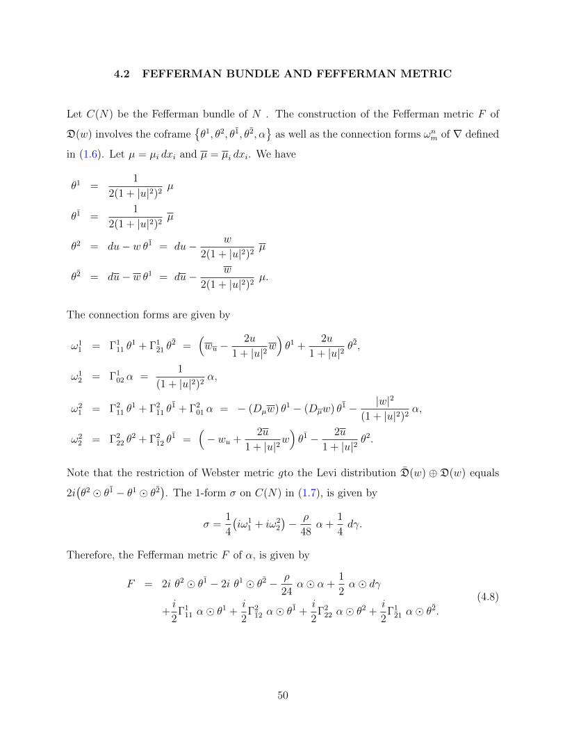
4.2 FEFFERMAN BUNDLE AND FEFFERMAN METRIC
Let C(N) be the Fefferman bundle of N . The construction of the Fefferman metric F of
D(w) involves the coframeθ1, θ2, θ1, θ2, α
as well as the connection forms ωnm of ∇ defined
in (1.6). Let µ = µi dxi and µ = µi dxi. We have
θ1 =1
2(1 + |u|2)2µ
θ1 =1
2(1 + |u|2)2µ
θ2 = du− w θ1 = du− w
2(1 + |u|2)2µ
θ2 = du− w θ1 = du− w
2(1 + |u|2)2µ.
The connection forms are given by
ω11 = Γ1
11 θ1 + Γ1
21 θ2 =
(wu −
2u
1 + |u|2w)θ1 +
2u
1 + |u|2θ2,
ω12 = Γ1
02 α =1
(1 + |u|2)2α,
ω21 = Γ2
11 θ1 + Γ2
11 θ1 + Γ2
01 α = − (Dµw) θ1 − (Dµw) θ1 − |w|2
(1 + |u|2)2α,
ω22 = Γ2
22 θ2 + Γ2
12 θ1 =
(− wu +
2u
1 + |u|2w)θ1 − 2u
1 + |u|2θ2.
Note that the restriction of Webster metric gto the Levi distribution D(w) ⊕ D(w) equals
2i(θ2 θ1 − θ1 θ2
). The 1-form σ on C(N) in (1.7), is given by
σ =1
4
(iω1
1 + iω22
)− ρ
48α +
1
4dγ.
Therefore, the Fefferman metric F of α, is given by
F = 2i θ2 θ1 − 2i θ1 θ2 − ρ
24α α +
1
2α dγ
+i
2Γ1
11 α θ1 +i
2Γ2
12 α θ1 +
i
2Γ2
22 α θ2 +i
2Γ1
21 α θ2.
(4.8)
50

Note that Γ212 = −(Γ1
11) and Γ222 = −(Γ1
21). The matrix representation of F corresponding
to the basis θ1, θ1, θ2, θ2, α, dγ is
[F ] =
0 0 0 −i i4Γ1
11 0
0 0 i 0 − i4(Γ1
11) 0
0 i 0 0 − i4(Γ1
21) 0
−i 0 0 0 i4Γ1
21 0
i4Γ1
11 − i4(Γ1
11) − i4(Γ1
21) i
4Γ1
21 − 124ρ 1
4
0 0 0 0 14
0
.
The entry Fij equals F (ui, uj), where the vectors uj’s are:
u1 = X1, u2 = X1, u3 = X2, u4 = X2, u5 = T and u6 =∂
∂γ. (4.9)
To be more specific, we have
F (X1, T ) =i
4Γ1
11 =i
4
(wu −
2u
1 + |u|2w),
F (X2, T ) =i
4Γ1
21 =iu
2(1 + |u|2),
F (T, T ) = − ρ
24and F
(T,
∂
∂γ
)=
1
4.
Moreover, the inverse of [F ] is:
[F−1] =
0 0 0 i 0 Γ121
0 0 −i 0 0 (Γ121
)
0 −i 0 0 0 (Γ111)
i 0 0 0 0 Γ111
0 0 0 0 0 4
Γ121 (Γ1
21) (Γ1
11) Γ111 4
23ρ− 2iΓ1
11Γ121
+2i(Γ111) (Γ1
21)
.
Since the signature of g on N is (+ + +−−), the signature of F is (+ + +−−−).
51

We proceed to consider the Levi-Civita connection ∇ of F on C(N). Let ∇uiuj = Γkij uk.
The Christoffel symbol Γkij is obtained by (1.8). In terms of the connection forms ωji ,
∇ui = ωji ⊗ uj with ωji (uk) = Γjki.
To obtain the Riemann tensor of ∇, we have to find most of the connection forms defined
by (1.13). In the following, we set
y = 1 + |u|2, Γ111 = wu −
2u
yw, Γ2
11 = −Dµw, Γ201 = −|w|
2
y2, (4.10)
Moreover, Γ111 and Γ2
11 satisfy the identities
DX1Γ1
11 = DµΓ111 + 2Γ2
01 and DuΓ211 =
2u
yΓ2
11 − 2D v|v|w (4.11)
respectively. The exterior derivatives, dθ1, dθ1, dθ2, dθ2 and dα are given by
dθ1 =2u
yθ1 ∧ θ2 +
1
y2θ2 ∧ α +
w
y2θ1 ∧ α,
dθ1 =2u
yθ1 ∧ θ2 +
1
y2θ2 ∧ α +
w
y2θ1 ∧ α,
dθ2 = Γ211 θ
1 ∧ θ1 − Γ212 θ
1 ∧ θ2 + Γ201 θ
1 ∧ α + (D v|v|w) θ1 ∧ α− w
y2θ2 ∧ α,
dθ2 = −Γ211 θ
1 ∧ θ1 + Γ111 θ
1 ∧ θ2 + (D v|v|w) θ1 ∧ α + Γ2
01 θ1 ∧ α− w
y2θ2 ∧ α,
dα = 2 θ1 ∧ θ2 + 2 θ1 ∧ θ2.
List of the connection forms ωnm of ∇:
ω11 =
1
2Γ1
11 θ1 − 1
4Γ2
12 θ1 +
u
2yθ2 +
3u
2yθ2 +
(φw8
+iρ
12
)α +
i
4dγ
ω21 =
1
4Γ1
11 θ1
ω31 = Γ2
11 θ1 + Γ2
11 θ1 − 1
4Γ1
11 θ2 −
(1
8DX1
Γ111 +
1
8DX1Γ1
11 +u
4y2Γ2
11 +u
4y2Γ2
11
)α
ω41 =
1
4Γ1
11 θ2
ω51 = θ2
52

ω61 =
(iDX1Γ1
11 − 4iD v|v|w − i
2(Γ1
11)2 +2iu
yΓ2
11
)θ1
+( i
2DX1
Γ111 −
i
2DX1Γ1
11 +iu
yΓ2
11 −iu
yΓ2
11
)θ1 +
(2iw
y2− iu
yΓ1
11
)θ2
+( i
2wuu −
iu
ywu
)θ2 + Γ6
51 α +1
4Γ1
11 dγ
ω13 =
u
2yθ1 +
1
2y2α
ω23 = − u
2yθ1
ω33 = −1
4Γ1
11 θ1 +
3
4Γ2
12 θ1 − u
yθ2 − u
2yθ2 −
( iρ24
+φw8
)α +
i
4dγ
ω43 = − u
2yθ2
ω53 = −θ1
ω63 =
(2iw
y2− iu
yΓ1
11
)θ1 +
(− i
2wuu +
iu
ywu
)θ1 + Γ6
53 α−u
2ydγ
ω15 =
( iρ12
+φw8
)θ1 − w
y2θ1 − 1
2y2θ2 +
( i
48Duρ+
1
4y2Γ2
12 +uw
2y3
)α
ω35 = −
(1
8DX1Γ1
11 +1
8DX1
Γ111 +
u
4yΓ2
11 +u
4yΓ2
11 −1
4Γ2
01
)θ1 − (D v
|v|w) θ1
−( iρ
24+φw8
)θ2 +
w
y2θ2 −
( i
48DX1
ρ+1
4D v
|v|Duw +
w
4y2Γ1
11 +u
2yΓ2
01
)α
ω55 = 0
ω65 = Γ6
15 θ1 + Γ6
25 θ1 + Γ6
35 θ2 + Γ6
45 θ2 + Γ6
55 α
ω16 =
i
4θ1
ω26 = − i
4θ1
ω36 =
i
4θ2
ω46 = − i
4θ2
ω56 = 0
ω66 =
1
4Γ1
11 θ1 − 1
4Γ2
12 θ1 − u
2yθ2 − u
2yθ2
53

We skip some of the most complicated Christoffel symbols here, e.g. Γ651. Other unlisted
connection 1-forms can be obtained by the complex conjugation of a 1-form above.
Let R be the curvature tensor of ∇ according to (1.9) and (1.10). It means
R(ui, uj)uk = Rlijkul and Rijkl = F
(R(ui, uj)uk, ul
).
Also, we let Ric be the Ricci tensor and S be the scalar curvature of ∇ as in (1.11) and
(1.12). The raise-index of Ric is denoted by Ric] with Ric](ui) = Rji uj. From Theorem 1.4,
we immediately have
S =5
3ρ =
5i
3
(φw − (φw)
),
where φw is defined in (4.4). The curvature forms of R are denoted by Ωnm, which are given
in (1.14) with Ωnm = dωnm − ωkm ∧ ωlk.
Following (1.14) and (1.15), we let W be the Weyl curvature tensor of ∇. In particular
W(ui, uj)uk = W lijk ul and Wijkl = F
(W(ui, uj)uk, ul
).
4.3 FURTHER RESULTS WHEN M IS FLAT
Theorem 4.6. Suppose D(w) is a CR structure on the twistor CR manifold N over a flat
space M . Associated with the contact form α (4.2), let F be the Fefferman metric of D(w)
on C(N) and S the scalar curvature of F .
Suppose w is holomorphic in u at the point u = 0. Then, S = 0 if and only if
w(x, u) = λ0(x) + λ1(x)u+K(x)u2 − λ1(x)u3 + λ0(x)u4 (4.12)
for λ0, λ1 ∈ C∞(M,C) and K ∈ C∞(M,R).
54
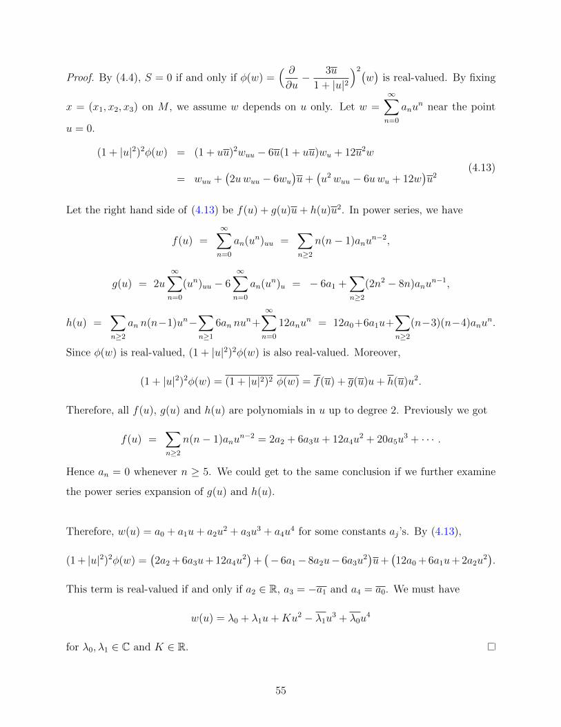
Proof. By (4.4), S = 0 if and only if φ(w) =( ∂∂u− 3u
1 + |u|2)2(
w)
is real-valued. By fixing
x = (x1, x2, x3) on M , we assume w depends on u only. Let w =∞∑n=0
anun near the point
u = 0.
(1 + |u|2)2φ(w) = (1 + uu)2wuu − 6u(1 + uu)wu + 12u2w
= wuu +(2uwuu − 6wu
)u+
(u2wuu − 6uwu + 12w
)u2
(4.13)
Let the right hand side of (4.13) be f(u) + g(u)u+ h(u)u2. In power series, we have
f(u) =∞∑n=0
an(un)uu =∑n≥2
n(n− 1)anun−2,
g(u) = 2u∞∑n=0
(un)uu − 6∞∑n=0
an(un)u = − 6a1 +∑n≥2
(2n2 − 8n)anun−1,
h(u) =∑n≥2
an n(n−1)un−∑n≥1
6an nun+
∞∑n=0
12anun = 12a0+6a1u+
∑n≥2
(n−3)(n−4)anun.
Since φ(w) is real-valued, (1 + |u|2)2φ(w) is also real-valued. Moreover,
(1 + |u|2)2φ(w) = (1 + |u|2)2 φ(w) = f(u) + g(u)u+ h(u)u2.
Therefore, all f(u), g(u) and h(u) are polynomials in u up to degree 2. Previously we got
f(u) =∑n≥2
n(n− 1)anun−2 = 2a2 + 6a3u+ 12a4u
2 + 20a5u3 + · · · .
Hence an = 0 whenever n ≥ 5. We could get to the same conclusion if we further examine
the power series expansion of g(u) and h(u).
Therefore, w(u) = a0 + a1u+ a2u2 + a3u
3 + a4u4 for some constants aj’s. By (4.13),
(1 + |u|2)2φ(w) =(2a2 + 6a3u+ 12a4u
2)
+(− 6a1− 8a2u− 6a3u
2)u+
(12a0 + 6a1u+ 2a2u
2).
This term is real-valued if and only if a2 ∈ R, a3 = −a1 and a4 = a0. We must have
w(u) = λ0 + λ1u+Ku2 − λ1u3 + λ0u
4
for λ0, λ1 ∈ C and K ∈ R.
55

As a remark, the torsion function w in (3.13) satisfies the condition (4.11). In fact, if both
λ0, λ1 and K are constant functions in (4.11), we obtain a further result that the Weyl tensor
W vanishes. (Theorem 7.3)
In our exploration for the properties of D(w), computational work shows that the Chern
tensor (4.7) coincides with the Weyl tensor on D ⊕D, when M is a flat space or a general
3-manifold. However, the statement that ‘C =W ’ is a rather general result in CR geometry.
We include a direct proof of this statement when M is flat for an extra reference.
As a preliminary, we find out the components of Ric]. We follow the notation in (4.10).
R11 =
7ρ
12− iφw
2, R2
1 = −4iw
y2, R3
1 =i
2DX1
Γ111 +
i
2DX1(Γ1
11) +iu
yΓ2
11 +iu
yΓ2
11,
R41 = −4iD v
|v|w, R5
1 = iΓ111, R1
3 =2i
y2, R2
3 = 0, R33 =
i
2φw +
ρ
12,
R43 =
4iw
y2, R5
3 = −2iu
y, R6
3 =6
y2Γ1
11+i
3Duρ−
u
yφw−
iu
3yρ, R1
5 =1
12Duρ+
i
y2(Γ1
11)− 2iu
y3w,
R55 =
ρ
12, R1
6 = R26 = R3
6 = R46 = 0, R5
6 = 1, R66 =
ρ
4.
The terms R61, R3
5 and R65 are skipped here because of their complexity. Other components
of Rji could be found by complex conjugation, e.g. R1
2 = R21.
Theorem 4.7. Let W(X, Y, Z,W ) = F(W(X, Y )Z,W
)for any tangent vectors X, Y, Z,W
on C(N). Let C is the (0,4)-Chern tensor of D(w) given by (4.7). Then,
Cmnkl = W(Xm, Xn, Xk, X l
)for every m,n, k, l = 1, 2.
56

Under the indexing of Wijkl’s with respect to the basis of uj’s (4.9), we have
W1212 =W(X1, X1, X1, X1), W1234 =W(X1, X1, X2, X2), W1515 =W(X1, T,X1, T )
and so on. We would follow the items in Proposition 4.5 to prove Theorem 4.7.
Proof. Step 1: Show that W(X1,X2,Z1,Z2) = 0 for any Z1,Z2 ∈ D⊕D.
It suffices to show that W1313, W1312, W1314, W1323, W1324 and W1334 are zero. We quote the
Sparling condition [6] [18] that ι ∂∂γW = 0, which implies W5
ijk =Wijk6 F65 = 0.
R2131 = 2
(dω2
1 − ωk1 ∧ ω2k
)(X1, X2) = 0
R3131 = 2
(dω3
1 − ωk1 ∧ ω3k
)(X1, X2)
= −DuΓ211 +
2u
yΓ2
11 +1
16(Γ1
11)2 −D v|v|w
= D v|v|w +
1
16(Γ1
11)2
R1131 = 2
(dω1
1 − ωk1 ∧ ω1k
)(X1, X2) =
w
y2+
u
8yΓ1
11
R4132 = 2
(dω4
2 − ωk2 ∧ ω4k
)(X1, X2) = −DuΓ
211 +
2u
yΓ2
11 −D v|v|w = D v
|v|w
R3132 = 2
(dω3
2 − ωk2 ∧ ω3k
)(X1, X2)
=1
4DX1(Γ1
11)− 1
16|Γ1
11|2 −1
2Γ2
01 −1
4Dµ(Γ1
11)
= − 1
16|Γ1
11|2
R3133 = 2
(dω3
3 − ωk3 ∧ ω3k
)= − w
y2− u
8yΓ1
11
57

Therefore, we have the following W lijk’s:
W2131 = R2
131 = 0
W3131 = R3
131 +1
4R11 = D v
|v|w +
1
16(Γ1
11)2 +1
4
(− 4D v
|v|w − 1
4(Γ1
11)2)
= 0
W1131 = R1
131 −1
4R13 =
w
y2+
u
8yΓ1
11 −1
4
( u2ywu −
w
y+
5w
y2
)=
w
y2+
w
4y2− 5w
4y2= 0
W4132 = R4
132 −i
4R4
1 = D v|v|w − i
4
(− 4iD v
|v|w)
= 0
W3132 = R3
132 −i
4R3
1 +1
4R12
= − 1
16|Γ1
11|2 −i
4
( i2DX1
Γ111 +
i
2DX1(Γ1
11) +iu
yΓ2
11 +iu
yΓ2
11
)+
1
4
(− 1
2DX1
Γ111 −
1
2DX1(Γ1
11)− u
yΓ2
11 −u
yΓ2
11 +1
4|Γ1
11|2)
= 0
W3133 = R3
133 +1
4R13 = − w
y2− u
8yΓ1
11 +1
4
( u2y
Γ111 +
4w
y2
)= 0
As a result, W1313 = W1312 = W1314 = W1323 = W1324 = W1334 = 0. It implies that
W(X1, X2, Z1, Z2) or W(X1, X2, Z1, Z2) is zero whenever Z1, Z2 are on D⊕D.
Step 2: Show that W1434 and W3434 are zero.
R1143 = 2
(dω1
3 − ωk3 ∧ ω1k
)(X1, X2) =
1
2y2+|u|2
4y2
R1343 = 2
(dω1
3 − ωk3 ∧ ω1k
)(X2, X2) = 0
So we have
W1143 = R1
143 −1
4R34 =
1
2y2+|u|2
4y2− 1
4
(2 + |u|2
y2
)= 0,
W1343 = R1
343 = 0.
58

Therefore,W1434 =W3434 = 0 are zero. Note thatW2334 = −W1434 = 0. All ofW1434,W3234,
W3414, W3432 and W3434 become zero, and they correspond to C1222, C2122, C2212, C2221 and
C2222 respectively.
Step 3: Show that W1234 = −ρ6
.
We first use the fact that tr(W) = 0, so∑
j,kW1jk4Fjk = 0. Since W1144 =W1324 = 0, we
have W1234 =W1414. Moreover, we may consider the Bianchi identity
W1234 +W2314 +W3124 = 0.
It gives W1432 = W1234. Once we establish that W1234 = −ρ6
, the coefficients W1414, W1432,
W3214,W3232 andW3412 are of the same value, which correspond to C1122, C1212, C1221, C2112,
C2121 and C2211 respectively.
R1123 = 2
(dω1
3 − ωk3 ∧ ω1k
)(X1, X1)
= −DX1
( u2y
)− u
8y(Γ1
11)− u
8y(Γ1
11)− 3u
8y(Γ1
11)− 1
8φw
− iρ12− u2w
2y2+
1
8φw +
u
2y(Γ1
11)
=(u2w
2y2
)− 5u
8y(Γ1
11)− iρ
12− u2w
2y2+
u
2y(Γ1
11) = − iρ
12− u
8y(Γ1
11)
Therefore,
W1123 = R1
123 −i
4R1
1 −1
4R23 +
i
20S
=(− iρ
12− u
8yΓ1
11
)− i
4
(7ρ
12− i
2φw
)− 1
4
(− 1
12wuu −
1
2φw +
1
12φw
)+iρ
12
= − 7i
48ρ− 1
48φw +
1
48wuu −
u
8y
(wu −
2u
yw)
=7
48
(φw − φw
)− 1
48φw +
1
48φw =
1
6
(φw − φw
).
It implies that W1234 = W1123F14 = − ρ
6.
59

Step 4: Show that W1214 equals C1112.
Note that for any vectors Z1, Z2 on D⊕D, W(X1, X1, Z1, Z2
)= −W
(X1, X1, Z1, Z2
). It
implies that W1214 = −W1223. Hence, W1214, W1232, W1412 and W3212 equal C1112, C1121,
C1211 and C2111 respectively. From Proposition 4.5, these coefficients of the Chern tensor
equal C1112, which could be written as
C1112 =i
2
(DX1
Γ111 +
2u
yΓ2
11 −DX1(Γ111)− 2u
yΓ2
11
).
R1121 = 2
(dω1
1 − ωk1 ∧ ω1k
)(X1, X1)
=(− 1
2DX1
Γ111 +
1
4DX1(Γ1
11) +u
2yΓ2
11 −3u
2yΓ2
11
)+
1
16|Γ1
11|2 +u
2yΓ2
11
+(− 1
8DX1
Γ111 +
1
8DX1(Γ1
11)− u
4yΓ2
11 +u
4yΓ2
11
)= −5
8DX1
Γ111 +
3
8DX1(Γ1
11) +1
16|Γ1
11|2 +3u
4yΓ2
11 −5u
4yΓ2
11
So we have
W1121 = R1
121 −1
4R12
= −5
8DX1
Γ111 +
3
8DX1(Γ1
11) +1
16|Γ1
11|2 +3u
4yΓ2
11 −5u
4yΓ2
11
−1
4
(− 1
2DX1
Γ111 −
1
2DX1(Γ1
11)− u
yΓ2
11 −u
yΓ2
11 +1
4|Γ1
11|2)
= −1
2DX1
Γ111 +
1
2DX1(Γ1
11)− u
yΓ2
11 +u
yΓ2
11.
Therefore,
W1214 =i
2
(DX1
Γ111 −DX1(Γ1
11) +2u
yΓ2
11 −2u
yΓ2
11
)= C1112.
60

Step 5: Show that W1212 = C1111.
Recall that C1111 = iDX1Γ211 − iDX1
Γ211 + iΓ2
11 (Γ111)− iΓ2
11Γ111.
R3121 = 2
(dω3
1 − ωk1 ∧ ω3l
)(X1, X1)
= −DX1Γ2
11 +DX1Γ211 −
1
4Γ1
11 Γ211 +
(− 1
2Γ1
11 Γ211 +
1
4(Γ1
11) Γ211
)+(3
4Γ2
11 (Γ111)− 1
4Γ2
11 Γ111
)= −DX1
Γ211 +DX1Γ2
11 − Γ111 Γ2
11 + (Γ111) Γ2
11
Therefore, W3121 = R3
121. Also,
W1212 = − iDX1Γ2
11 + iDX1Γ211 − iΓ1
11 Γ211 + i (Γ1
11) Γ211 = C1111.
61
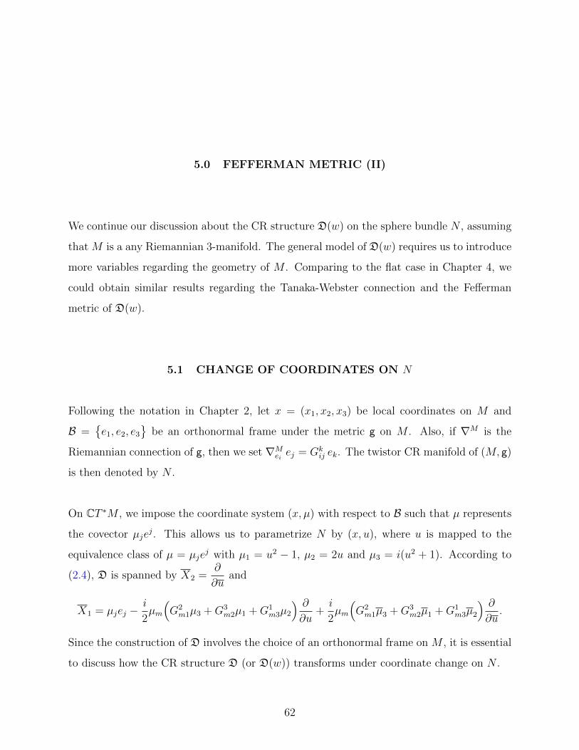
5.0 FEFFERMAN METRIC (II)
We continue our discussion about the CR structure D(w) on the sphere bundle N , assuming
that M is a any Riemannian 3-manifold. The general model of D(w) requires us to introduce
more variables regarding the geometry of M . Comparing to the flat case in Chapter 4, we
could obtain similar results regarding the Tanaka-Webster connection and the Fefferman
metric of D(w).
5.1 CHANGE OF COORDINATES ON N
Following the notation in Chapter 2, let x = (x1, x2, x3) be local coordinates on M and
B =e1, e2, e3
be an orthonormal frame under the metric g on M . Also, if ∇M is the
Riemannian connection of g, then we set ∇Meiej = Gk
ij ek. The twistor CR manifold of (M, g)
is then denoted by N .
On CT ∗M , we impose the coordinate system (x, µ) with respect to B such that µ represents
the covector µjej. This allows us to parametrize N by (x, u), where u is mapped to the
equivalence class of µ = µjej with µ1 = u2 − 1, µ2 = 2u and µ3 = i(u2 + 1). According to
(2.4), D is spanned by X2 =∂
∂uand
X1 = µjej −i
2µm
(G2m1µ3 +G3
m2µ1 +G1m3µ2
) ∂∂u
+i
2µm
(G2m1µ3 +G3
m2µ1 +G1m3µ2
) ∂∂u.
Since the construction of D involves the choice of an orthonormal frame on M , it is essential
to discuss how the CR structure D (or D(w)) transforms under coordinate change on N .
62

Let B′ =f1, f2, f3
be another orthonormal frame on M . We have fj = akj(x) ek with
[akj(x)] in SO(3,R) for every x. It also means that ek = ajk fj = akj fj, and for the
coframe of B′, fm = alm el.
Let (x, γ) be the coordinate system on T ∗M with respect to the frame B′. Define Φ to be the
transition map from (x, µ) to (x, γ). If we assume γm fm = µl e
l = γm alm el, then
µl = alm γm and γm = alm µl.
Suppose T kij = g(∇Mfifj, fk
). The horizontal vector field µh (2.1) is defined by
µh = µj ej − µmGlmk µk
∂
∂µl− µmGl
mk µk∂
∂µl
at (x, µ). If γ = Φ(µ), then γh = dΦ(µh) with
γh = γj fj − γm T lmk γk∂
∂γl− γm T lmk γk
∂
∂γl
at the point (x, γ) under the coordinate system with respect to B′.
The space of null covectors N can be parametrized by the rational parametrization f ,
f : C2\0→ Nx,(µ1, µ2, µ3
)= f(s, t) =
(s2 − t2, 2st, i(s2 + t2)
)at the point x in M . Let Sx be the complex plane of (s, t) defined above at x. S =
⋃x∈M Sx
is a complex vector bundle of rank 2 over M , called the spinor bundle of M [5]. With respect
to B′, we construct another rational parametrization
h : C2\0→ Nx,(γ1, γ2, γ3
)= h(s′, t′) =
(s′2 − t′2, 2s′t′, i(s′2 + t′2)
).
The transition map φ from (s, t) to (s′, t′) is defined in a way that this diagram commutes.
(Sx, (s, t)
)φ−→
(Sx, (s′, t′)
)f ↓ ↓ h(
Nx, (µ1, µ2, µ3)
)Φ−→
(Nx, (γ
1, γ2, γ3))
63

For any matrix P in SU(2), P is in the form of
P =
b −c
c b
for complex numbers b and c such that |b|2 + |c|2 = 1. We may consider the 2:1 covering
map q from SU(2) to SO(3,R) defined by
q(P ) =
1
2(b2 − c2 + b2 − c2) −bc− bc − i
2(b2 − c2 − b2 + c2)
bc+ bc |b|2 − |c|2 −i(bc− bc)
i
2(b2 + c2 − b2 − c2) i(−bc+ bc)
1
2(b2 + c2 + b2 + c2)
.
Proposition 5.1. Let (s′, t′) and (s, t) be two coordinate systems on S such that on Sx, s′
t′
=
b −c
c b
s
t
.
Let P =
[b −c
c b
]in SU(2). Then, on the fibre Nx, we have
s′2 − t′2
2s′t′
i(s′2 + t′2)
=
[q(P )
] s2 − t2
2st
i(s2 + t2)
.for every (s, t) on Sx.
Under the coordinate transformation γj = akj(x)µk on T ∗M , we let A = [aij(x)] and then
find a matrix function P ,
P (x) =
b(x) −c(x)
c(x) b(x)
such that |b|2 + |c|2 = 1 and q(P ) = AT at every x. If φ is defined by s′ = bs − ct and
t′ = cs+ bt on Sx, then we obtain (h φ)(s, t) = Φ f(s, t) for every (s, t).
64

Back to the manifold N , with respect to the rational parametrization h given by B′, we
define a complex parameter v on N such that s′ = v and t′ = 1. The parameter v represents
the equivalence class of the covector (v2 − 1)f 1 + 2vf 2 + i(v2 + 1)f 3.
Let v = φ(u) be the transition map from (x, u) to (x, v). Indeed,
v =s′
t′=
bu− ccu+ b
.
Using Proposition 5.1, we get to the equation
t′2
v2 − 1
2v
i(v2 + 1)
=
s′2 − t′2
2s′t′
i(s′2 + t′2)
=
a11 a21 a31
a12 a22 a32
a13 a23 a33
u2 − 1
2u
i(u2 + 1)
.Let v1 = v2 − 1, v2 = 2v and v3 = i(v2 + 1). The differential map dφ at (x, u)is given by
dφ( ∂∂u
)=
1
(cu+ b)2
∂
∂v,
dφ(X1
)= t′2
[vjfj−
ivm2
(T 2m1v3+T 3
m2v1+T 1m3v2
) ∂∂v
+ivm
2
(T 2m1v3+T 3
m2v1+T 1m3v2
) ∂∂v
].
Therefore, in the coordinates (x, v), the CR structure D is spanned by Y 2 =∂
∂vand
Y 1 = vjfj −ivm
2
(T 2m1v3 + T 3
m2v1 + T 1m3v2
) ∂∂v.
In the next step, we introduce the torsion function w(x, u) to the model and consider the
CR structure D(w). At the point (x, u), D(w) is spanned by∂
∂uand
X = µjej −i
2µm(G2m1µ3 +G1
m3µ2 +G3m2µ1
) ∂∂u
+ w∂
∂u+ w
∂
∂u.
The image of X by dφ is the vector
dφ(X1 + w(x, u)
∂
∂u
)= Y1 + w
(x, φ−1(v)
) 1
t′2∂
∂v.
65

Note that u = φ−1(v) =−bv − ccv − b
. In the coordinate system (x, v) with respect to B′, D(w)
is spanned by∂
∂vand
Y 1 = vjfj −ivm
2
(T 2m1v3 + T 3
m2v1 + T 1m3v2
) ∂∂v
+ (cv − b)4w(x,−bv − ccv − b
) ∂∂v. (5.1)
The equation (5.1) allows us to keep the rational parametrization on N in the same style
while using different orthonormal frames on M to analyze D(w).
For example, the complex parameter u could not cover every point on Nx, so we need to set
v =1
uto cover the missing point. By Proposition 5.1, we may let b = 0 and c = i, which
also means to consider the orthonormal frame f1 = e1, f2 = −e2 and f3 = −e3. In the
coordinates (x, v), v = 0 refers to the missing covector −e1 − i e3. The transition map from
(x, u) to (x, v) sends D(w) under B to the CR structure D(w′) under B′ with
w′(x, v) = v4 w(x,
1
v
).
In this way, our results from the local model can be applied to the coordinate chart of (x, v).
In addition to transitions between orthonormal frames, change of coordinates on N can be
realized by a transition between conformal moving frames. Suppose g = λ2 g for a positive
function λ on M . Since [g] = [g], N (equipped with D) is also the twistor CR manifold of
(M, g).
Let ej = 1λej (ej = λ ej) and so B′′ =
e1, e2, e3
is an orthonormal frame on M under g.
We also let ∇ be the Riemannian connection of g with ∇ei ej = Gkij ek.
B′′ defines a coordinate system (γ1, γ2, γ2) on CT ∗M . The change of coordinates from γ to
µ is given by µj = λ γj. The rational parametrization on N with respect to B′′ maps the
complex parameter v to [γj ej] = [µje
j]. It means that v = u.
66

Suppose we begin with the CR structure D(w, g) on N which is described by
Y 1 = µj ej −i
2µm
(G2m1 µ3 + G3
m2 µ1 + G1m3 µ2
) ∂∂u
+ w∂
∂u
Y 2 =∂
∂u
α =u+ u
1 + |u|2e1 +
1− |u|2
1 + |u|2e2 +
i(u− u)
1 + |u|2e3
(5.2)
in the coordinates (x, u). Here µ1 = u2 − 1, µ2 = 2u, µ3 = i(u2 + 1).
If we let [ei, ej] = Akij ek and [ei, ej] = Bkij ek, then
[ei, ej] =λjλ2ei −
λiλ2ej +
1
λ2[ei, ej] =⇒ Bk
ij =δik λj − δjk λi
λ2+
1
λAkij.
We denote ej(λ) by λj above. By Koszul formula,
Gkij =
1
2
(−Bj
ik −Bijk +Bk
ij
)=
1
λ2
(δik λj − δij λk
)+
1
λGkij.
Therefore, in the local model (5.2), we get
f = − i
2
(G2m1 µ3 + G3
m2 µ1 + G1m3 µ2
)= − i
2λ
(G2m1 µ3 +G3
m2 µ1 +G1m3 µ2
)=
1
λf.
It allows us to rewrite Y 1 (5.2) by Y 1 =1
λ
(µj ej + (f + λw)
∂
∂u
). Therefore, the model of
D(w, g) is equivalent to the model of D(λw, g), described by
X1 = µj ej −i
2µm
(G2m1 µ3 +G3
m2 µ1 +G1m3 µ2
) ∂∂u
+ λw∂
∂u
X2 =∂
∂u
α =u+ u
1 + |u|2e1 +
1− |u|2
1 + |u|2e2 +
i(u− u)
1 + |u|2e3
(5.3)
Note that the contact forms in (5.2) and (5.3) differ by a factor of λ.
67

5.2 THE LOCAL MODEL OF D(w): GENERAL CASE
On the sphere bundle N of M , we define the CR structure D(w) by substituting the torsion
function w for the term uT ·C · q in (3.7). D(w) is then spanned by X2 =∂
∂uand
X1 = µj ej −i
2µm
(G2m1 µ3 +G3
m2 µ1 +G1m3 µ2
) ∂∂u
+ w∂
∂u
at (x, u) with µ1 = u2 − 1, µ2 = 2u and µ3 = i(u2 + 1). We let
f(x, u) = − i2µm
(G2m1 µ3 +G3
m2 µ1 +G1m3 µ2
). (5.4)
Since f is holomorphic in u, we can combine the coefficients of∂
∂uin X1.
On N , the local model of D(w) is described by
X1 = (u2 − 1) e1 + 2u e2 + i(u2 + 1) e3 + w(x, u)∂
∂u
X1 = (u2 − 1) e1 + 2u e2 − i(u2 + 1) e3 + w(x, u)∂
∂u
X2 =∂
∂u
X2 =∂
∂u
T =u+ u
1 + |u|2e1 +
1− |u|2
1 + |u|2e2 +
i(u− u)
1 + |u|2e3 + T4
∂
∂u+ T 4
∂
∂u.
(5.5)
Note that the actual torsion function is (w−f) under our setting. By the notation v = i µ×µ
and |v| = 2(1 + |u|2)2, we have
v1
|v|=
u+ u
1 + |u|2,
v2
|v|=
1− |u|2
1 + |u|2and
v3
|v|=i(u− u)
1 + |u|2.
So T =v
|v|+ T4
∂
∂u+ T 4
∂
∂u. The contact form of D(w) is chosen to be
α =v1
|v|e1 +
v2
|v|e2 +
v3
|v|e3. (5.6)
68

The exterior derivative of α is given by,
dα = − 1
(1 + |u|2)2
((µ1 du+ µ1 du) ∧ e1 + (µ2 du+ µ2 du) ∧ e2 + (µ3 du+ µ3 du) ∧ e3
)+( v1
|v|G2
11 −v2
|v|G1
22 −v3
|v|(G1
23 +G312))e1 ∧ e2
+(− v1
|v|(G1
23 +G231) +
v2
|v|G3
22 −v3
|v|G2
33
)e2 ∧ e3
+(− v1
|v|G3
11 −v2
|v|(G2
31 +G312) +
v3
|v|G1
33
)e3 ∧ e1.
Being the Reeb vector field corresponding to α, T is characterized by dα(T, ·) = 0, where
T4 = − 1
2
vm|v|
(Glmk µk
vl|v|
)= − i
2
vm|v|
(G2m1 µ3 +G1
m3 µ2 +G3m2 µ1
). (5.7)
The Levi-form of α is defined by L = −i dα. Its components are hαβ = L(Xα, Xβ). We have
h12 = −i, h21 = i and h22 = 0. The remaining coefficient is,
h11 = −|µ1|2G312 − |µ2|2G1
23 − |µ3|2G231
+1
2|v|
(G2
11 v1 v3 −G311 v1 v2 −G1
22 v3 v2 +G322 v2 v1 +G1
33 v2 v3 −G233 v1 v3
).
(5.8)
The inverse of h is given by h11 = 0, h12 = −i, h21 = i and h22 = −h11.
The coframe toX1, X1, X2, X2, T
consists of
θ1 =1
2(1 + |u|2)2
(µj e
j), θ1 =
1
2(1 + |u|2)2
(µj e
j),
θ2 = du− w θ1 − T4 α, θ2 = du− w θ1 − T 4 α,
together with the contact form α. Let g be the Webster metric associated with α, where
g = 2h11 θ1 θ1 + 2i θ2 θ1 − 2i θ1 θ2 + α α.
69
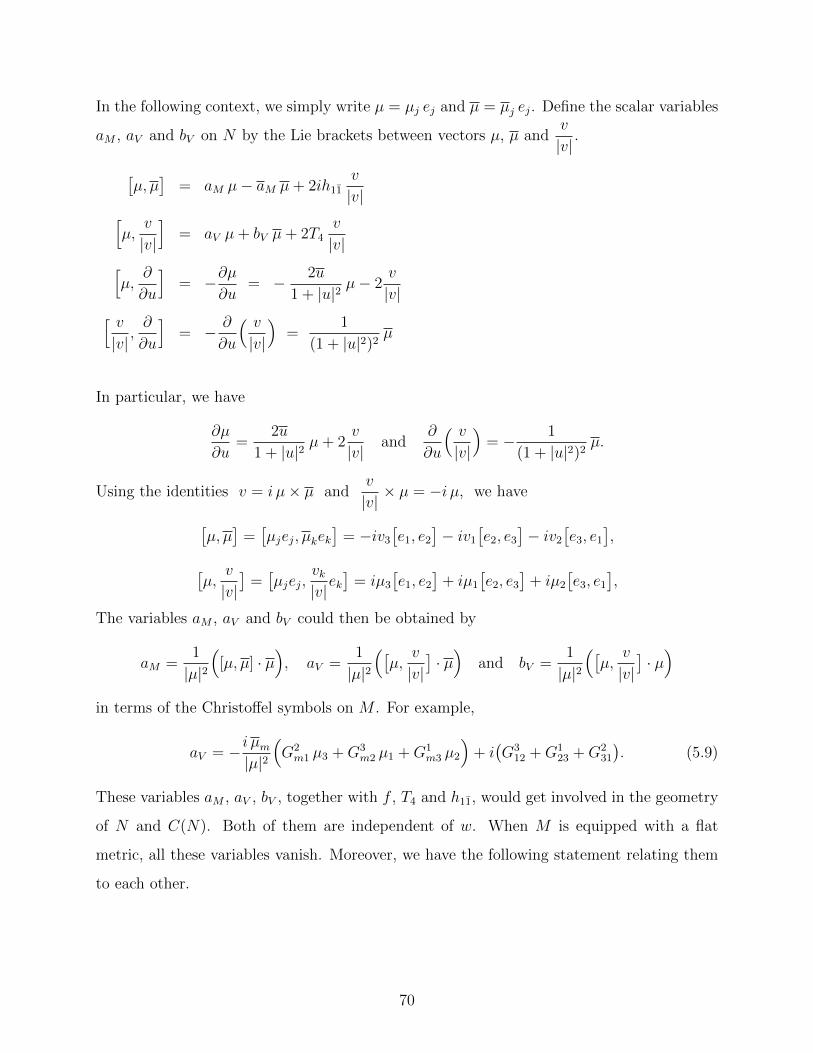
In the following context, we simply write µ = µj ej and µ = µj ej. Define the scalar variables
aM , aV and bV on N by the Lie brackets between vectors µ, µ andv
|v|.
[µ, µ
]= aM µ− aM µ+ 2ih11
v
|v|[µ,
v
|v|
]= aV µ+ bV µ+ 2T4
v
|v|[µ,
∂
∂u
]= −∂µ
∂u= − 2u
1 + |u|2µ− 2
v
|v|[ v|v|,∂
∂u
]= − ∂
∂u
( v|v|
)=
1
(1 + |u|2)2µ
In particular, we have
∂µ
∂u=
2u
1 + |u|2µ+ 2
v
|v|and
∂
∂u
( v|v|
)= − 1
(1 + |u|2)2µ.
Using the identities v = i µ× µ andv
|v|× µ = −i µ, we have
[µ, µ
]=[µjej, µkek
]= −iv3
[e1, e2
]− iv1
[e2, e3
]− iv2
[e3, e1
],
[µ,
v
|v|]
=[µjej,
vk|v|ek]
= iµ3
[e1, e2
]+ iµ1
[e2, e3
]+ iµ2
[e3, e1
],
The variables aM , aV and bV could then be obtained by
aM =1
|µ|2(
[µ, µ] · µ), aV =
1
|µ|2([µ,
v
|v|]· µ)
and bV =1
|µ|2([µ,
v
|v|]· µ)
in terms of the Christoffel symbols on M . For example,
aV = −i µm|µ|2
(G2m1 µ3 +G3
m2 µ1 +G1m3 µ2
)+ i(G3
12 +G123 +G2
31
). (5.9)
These variables aM , aV , bV , together with f , T4 and h11, would get involved in the geometry
of N and C(N). Both of them are independent of w. When M is equipped with a flat
metric, all these variables vanish. Moreover, we have the following statement relating them
to each other.
70
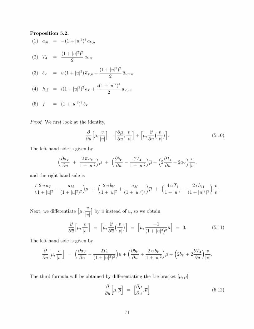
Proposition 5.2.
(1) aM = −(1 + |u|2)2 aV,u
(2) T4 =(1 + |u|2)2
2aV,u
(3) bV = u (1 + |u|2) aV,u +(1 + |u|2)2
2aV,u u
(4) h11 = i(1 + |u|2)2 aV +i(1 + |u|2)4
2aV,uu
(5) f = (1 + |u|2)2 bV
Proof. We first look at the identity,
∂
∂u
[µ,
v
|v|
]=[∂µ∂u,v
|v|
]+[µ,
∂
∂u
( v|v|)]. (5.10)
The left hand side is given by(∂aV∂u
+2u aV
1 + |u|2)µ +
(∂bV∂u− 2T4
1 + |u|2)µ+
(2∂T4
∂u+ 2aV
) v|v|,
and the right hand side is( 2u aV1 + |u|2
− aM(1 + |u|2)2
)µ +
( 2u bV1 + |u|2
+aM
(1 + |u|2)2
)µ +
( 4uT4
1 + |u|2− 2 i h11
(1 + |u|2)2
) v|v|.
Next, we differentiate[µ,
v
|v|]
by u instead of u, so we obtain
∂
∂u
[µ,
v
|v|
]=[µ,
∂
∂u
( v|v|)]
=[µ,
−1
(1 + |u|2)2µ]
= 0. (5.11)
The left hand side is given by
∂
∂u
[µ,
v
|v|
]=(∂aV∂u− 2T4
(1 + |u|2)2
)µ+
(∂bV∂u
+2u bV
1 + |u|2)µ+
(2bV + 2
∂T4
∂u
) v|v|.
The third formula will be obtained by differentiating the Lie bracket [µ, µ].
∂
∂u
[µ, µ
]=[∂µ∂u, µ]
(5.12)
71

By expansion, the left hand side is(∂aM∂u
+2u aM1 + |u|2
)µ −
(∂aM∂u
+2 i h11
(1 + |u|2)2
)µ +
(2aM + 2i
∂h11
∂u
) v|v|.
And the right hand side is( 2u aM1 + |u|2
− 2bV
)µ −
( 2u aM1 + |u|2
+ 2aV
)µ +
(4 i u h11
1 + |u|2− 4T 4
) v|v|.
We would apply equations (5.10), (5.11) and (5.12) to justify Proposition 5.2. For example,
the µ-coefficients of (5.10) give
aM = −(1 + |u|2)2 aV,u,
and the µ-coefficients of (5.9) implies that
T4 =(1 + |u|2)2
2aV,u.
Considering the µ-coefficients of (5.12), we get
bV = −1
2aM,u = − 1
2
∂
∂u
(− (1 + |u|2)2 aV,u
)= u (1 + |u|2) aV,u +
(1 + |u|2)2
2aV,u u.
For the last item, the v|v| -components of (5.10) gives
T4,u + 2aV =4uT4
1 + |u|2− 2 i h11
(1 + |u|2)2
(1 + |u|2)2 aV,uu + 2aV = − 2 i h11
(1 + |u|2)2
h11 = i (1 + |u|2)2 aV +i
2(1 + |u|2)4 aV,uu.
As a remark, h11 = L(X1, X1) is real-valued, so h11 = h11. By item (4), we have
aV + aV +1
2(1 + |u|2)2
(aV,uu + aV,uu
)= 0. (5.13)
72

We also derive relations between the u- or u-derivatives of aV by (5.10), (5.11) and (5.12).
Proposition 5.3.
(1) aV,uu =2
(1 + |u|2)2
(2i(G3
12 +G123 +G2
31) + aV − 2aV
)(2) aV,u u =
−2u
1 + |u|2(aV,u + aV,u
)− aV,u u
(3) aV,uuu = − 6u2
(1 + |u|2)2aV,u −
6u
1 + |u|2aV,uu
Proof. For the item(2), thev
|v|-component of (5.11) gives bV = −T4,u. By expansion,
u (1 + |u|2) aV,u +(1 + |u|2)2
2aV,u u = − u (1 + |u|2) aV,u −
(1 + |u|2)2
2aV,u u
aV,u u =−2u
1 + |u|2(aV,u + aV,u
)− aV,u u.
To prove the item (3), we look at the µ-coefficients of (5.11).
bV,u +2u
1 + |u|2bV = 3u2 aV,u + 3u (1 + |u|2) aV,u u +
(1 + |u|2)2
2aV,u uu = 0
=⇒ aV,uuu = − 6u2
(1 + |u|2)2aV,u −
6u
1 + |u|2aV,uu
Finally, We compare the µ-terms on both sides of (5.10).
bV,u −2T4
(1 + |u|2)2=
2ubV1 + |u|2
+aM
(1 + |u|2)2.
In terms of aV and its derivatives,
bV,u −2T4
(1 + |u|2)2=
(1 + 2|u|2
)aV,u + u (1 + |u|2) aV,uu + u (1 + |u|2) aV,u u
+(1 + |u|2)2
2aV,uuu − aV,u
2u bV1 + |u|2
+aM
(1 + |u|2)2=
(2|u|2 − 1
)aV,u + u (1 + |u|2) aV,u u.
73

Therefore,(1 + |u|2)2
2aV,uuu + u (1 + |u|2) aV,uu + 2aV,u − aV,u = 0
∂
∂u
(2aV − aV +
(1 + |u|2)2
2aV,uu
)= 0
=⇒ ∂
∂u
(2aV − aV +
(1 + |u|2)2
2aV,uu
)= 0.
By (5.13), we may substitute aV,uu with −aV,uu −2
(1 + |u|2)2(aV + aV ). So,
∂
∂u
(2aV − aV +
(1 + |u|2)2
2aV,uu
)= 0.
Hence we know that the expression 2aV − aV +(1 + |u|2)2
2aV,uu is independent of u or u.
At the point u = 0, which refers to µ1 = −1, µ2 = 0 and µ3 = i, we obtain
aV =i
2
(G3
12 +G231
)+ i G1
23 −1
2
(G2
11 +G233
),
aV = − i2
(G3
12 +G231
)− i G1
23 −1
2
(G2
11 +G233
),
aV,uu = −2i G123 + i G3
12 + i G231 +G2
11 +G233.
Therefore,
2aV − aV +(1 + |u|2)2
2aV,uu
=(
2aV − aV +(1 + |u|2)2
2aV,uu
)∣∣∣u=0
=(i G3
12 + i G231 + 2i G1
23 −G211 −G2
33
)+( i
2G3
12 +i
2G2
31 + i G123 +
1
2G2
11 +1
2G2
33
)+(− i G1
23 +i
2G3
12 +i
2G2
31 +1
2G2
11 +1
2G2
33
)= 2 i
(G3
12 +G123 +G2
31
),
which justifies the item (1) of Proposition 5.3.
74

The function f in (5.4) could be rewritten as
f = (1 + |u|2)2 bV = − u (1 + |u|2)3 aV,u −(1 + |u|2)4
2aV,u u. (5.14)
By Proposition 5.2 and 5.3, we would make use of the variables aM , aV , bV , h11, T4 to
express important variables on N . Moreover, we could replace these variables by aV and its
derivatives if need be.
In the following context, we follow the same notation (right before Proposition 4.1) about
directional derivatives of functions. If q = q(x, u, u) is a function on N , then Dµq, Dµq and
D v|v|q are the directional derivatives of q by µ, µ and v
|v| respectively.
We are ready the find the Lie brackets between X1, X2, X1, X2 and T of D(w) in (5.5).
Proposition 5.4.
[X1, X2] = − 2u
1 + |u|2X1 + 2T4X2 +
( 2uw
1 + |u|2+ 2T 4 − wu
)X2 − 2T
[X1, X1] = aM X1 − aM X1 +(Dµw + aM w + 2i h11 T4
)X2
+(−Dµw − aM w + 2i h11 T 4
)X2 − 2i h11 T
[X1, T ] =(bV −
w
(1 + |u|2)2
)X1 +
(aV −
2uT4
1 + |u|2)X1
+
(−D v
|v|w − T4wu +
(T4,u +
2uT4
1 + |u|2− aV
)w +DµT4
)X2
+(T 4,uw − bV w +
|w|2
(1 + |u|2)2+DµT 4
)X2
[X2, T ] = − 1
(1 + |u|2)2X1 + T4,uX2 +
( w
(1 + |u|2)2+ T 4,u
)X2
Also, [X1, X2] = [X2, X2] = 0.
75

5.3 THE SCALAR CURVATURE FORMULA
We denote the Tanaka-Webster connection of g by ∇, and define its Christoffel symbols in
the same style: ∇XmXn = ΓkmnXk, ∇XmXn = ΓkmnXk and ∇TXn = Γk0nXk. See equation
(1.1) for their formulas.
Proposition 5.5.
Γ111 = wu −
2uw
1 + |u|2− 2T 4
Γ211 = −Dµw + i h11wu −
(i∂h11
∂u+
2 i u h11
1 + |u|2+ aM
)w − iDµh11 − i aM h11
Γ212 = aM
Γ221 = −i ∂h11
∂u+
2 i u h11
1 + |u|2− 2T 4
Γ222 = − 2u
1 + |u|2
Γ112 = Γ1
21 = Γ122 = 0
Γ111 = −aM
Γ211 = −Dµw − aM w − 2 i h11 T4
Γ212 = −wu +
2uw
1 + |u|2+ 2T4
Γ121 =
2u
1 + |u|2
Γ221 = −2T4
Γ112 = Γ1
22 = Γ222 = 0
Γ101 = −aV +
2uT 4
1 + |u|2
Γ201 = − |w|2
(1 + |u|2)2+ bV w −DµT4 − w
∂T4
∂u
Γ102 =
1
(1 + |u|2)2
Γ202 = −∂T4
∂u
76

Note that we could express aM , T4 and aV in terms of the Christoffel symbols,
aM = Γ212, T4 = −1
2Γ2
21 and aV =1
2Γ2
21 Γ222 − Γ1
01.
Let R be the Riemann tensor of the Tanaka-Webster connection on N . Let
Rmnkl = θn
(R(Xk, X l)Xm
)according to (1.2). Also, we let ric be the Ricci tensor and ρ be the scalar curvature of ∇
defined by (1.3). Extending the result in Proposition 4.4, we may obtain a general formula
for the scalar curvature ρ.
Proposition 5.6. For Rmn = ric(Xm, Xn), we have the following.
R11 = −DµDuw −DµDuw +4u
1 + |u|2Dµw +
4u
1 + |u|2Dµw +
4|w|2
(1 + |u|2)2
+(1 + |u|2)2(wu aV,u + wu aV,u
)− 4(1 + |u|2)
(uw aV,u − uw aV,u
)+12i(1 + |u|2)2(aV − aV )
(G3
12 +G123 +G2
31
)− 8(1 + |u|2)2
(G3
12 +G123 +G2
31
)2
+(1 + |u|2)2(
4(aV − aV )2 +DµDuaV +DµDuaV +DµDuaV +DµDuaV
)−(1 + |u|2)4
(aV,u aV,u + aV,u aV,u − 2|aV,u|2
)R12 = −φw − 4i(G3
12 +G123 +G2
31) + 2aV − 6aV
R21 = −φw + 4i(G312 +G1
23 +G231)− 6aV + 2aV
R22 =4
(1 + |u|2)2
The term φw above is defined by (4.4). The scalar curvature ρ can be found by (1.3).
ρ = h11R11 + h12R21 + h21R12 + h22R22 = i(R12 −R21
)− h11R22
77
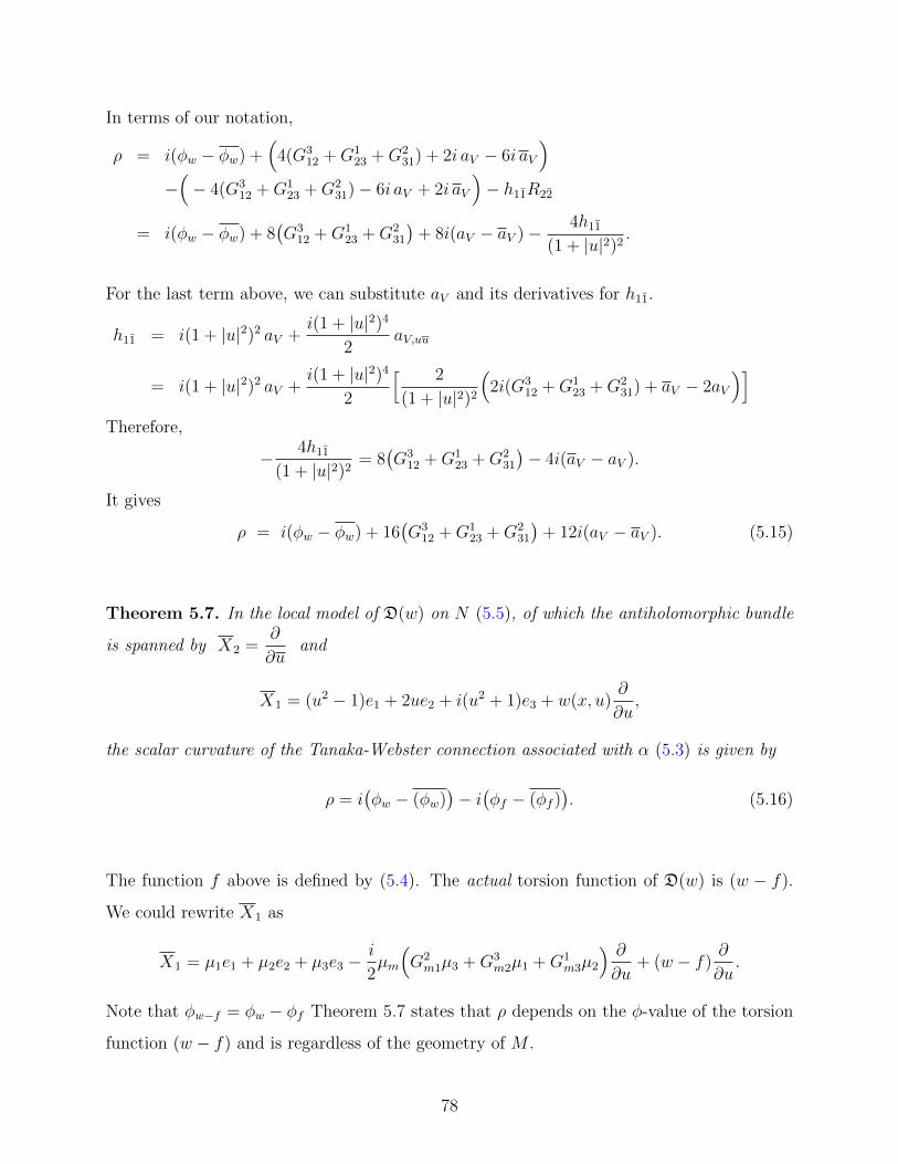
In terms of our notation,
ρ = i(φw − φw) +(
4(G312 +G1
23 +G231) + 2i aV − 6i aV
)−(− 4(G3
12 +G123 +G2
31)− 6i aV + 2i aV
)− h11R22
= i(φw − φw) + 8(G3
12 +G123 +G2
31
)+ 8i(aV − aV )− 4h11
(1 + |u|2)2.
For the last term above, we can substitute aV and its derivatives for h11.
h11 = i(1 + |u|2)2 aV +i(1 + |u|2)4
2aV,uu
= i(1 + |u|2)2 aV +i(1 + |u|2)4
2
[ 2
(1 + |u|2)2
(2i(G3
12 +G123 +G2
31) + aV − 2aV
)]Therefore,
− 4h11
(1 + |u|2)2= 8(G3
12 +G123 +G2
31
)− 4i(aV − aV ).
It gives
ρ = i(φw − φw) + 16(G3
12 +G123 +G2
31
)+ 12i(aV − aV ). (5.15)
Theorem 5.7. In the local model of D(w) on N (5.5), of which the antiholomorphic bundle
is spanned by X2 =∂
∂uand
X1 = (u2 − 1)e1 + 2ue2 + i(u2 + 1)e3 + w(x, u)∂
∂u,
the scalar curvature of the Tanaka-Webster connection associated with α (5.3) is given by
ρ = i(φw − (φw)
)− i(φf − (φf )
). (5.16)
The function f above is defined by (5.4). The actual torsion function of D(w) is (w − f).
We could rewrite X1 as
X1 = µ1e1 + µ2e2 + µ3e3 −i
2µm
(G2m1µ3 +G3
m2µ1 +G1m3µ2
) ∂∂u
+ (w − f)∂
∂u.
Note that φw−f = φw − φf Theorem 5.7 states that ρ depends on the φ-value of the torsion
function (w − f) and is regardless of the geometry of M .
78

Proof. We have to show that (5.15) implies (5.16). By comparison, it suffices to show
φf = 8i(G3
12 +G123 +G2
31
)− 6aV + 6aV .
We try to express f , fu and fuu in terms of lower derivatives of aV , which are aV,u, aV,u, aV,uu
and their complex conjugates. On the left hand side,
φf = fuu −6u fu
1 + |u|2+
12u2 f
(1 + |u|2)2.
We start from simplifying f .
f = −u (1 + |u|2)3 aV,u −(1 + |u|2)4
2aV,u u
= −u (1 + |u|2)3 aV,u −(1 + |u|2)4
2
[ −2u
1 + |u|2(aV,u + aV,u
)− aV,u u
]= u(1 + |u|2)3 aV,u +
(1 + |u|2)4
2aV,u u
The u-derivative of f is
∂f
∂u=
((1 + |u|2)3 + 3uu (1 + |u|2)2
)aV,u + u (1 + |u|2)3 aV,uu
+2u (1 + |u|2)3 aV,u u +(1 + |u|2)4
2aV,uuu
= (1 + |u|2)2(1 + 4|u|2) aV,u + 2u (1 + |u|2)3 aV,u u
+u (1 + |u|2)3 · 2
(1 + |u|2)2
(− 2i
(G3
12 +G123 +G2
31
)+ aV − 2aV
)+
(1 + |u|2)4
2· ∂∂u
[ 2
(1 + |u|2)2
(− 2i(G3
12 +G123 +G2
31) + aV − 2aV)]
= (1 + |u|2)2 (1 + 4|u|2) aV,u + 2u (1 + |u|2)3 aV,u u
+2u (1 + |u|2)(− 2i(G3
12 +G123 +G2
31) + aV − 2aV)
+(1 + |u|2)4
2
−4u
(1 + |u|2)3
(− 2i(G3
12 +G123 +G2
31) + aV − 2aV)
+2
(1 + |u|2)2
(aV,u − 2aV,u
)
= (1 + |u|2)2(1 + 4|u|2)aV,u + 2u(1 + |u|2)3aV,u u + (1 + |u|2)2aV,u − 2(1 + |u|2)2aV,u.
79

Therefore,
∂f
∂u= (1 + |u|2)2 (4|u|2 − 1) aV,u + (1 + |u|2)2 aV,u + 2u (1 + |u|2)3 aV,u u.
The second derivative of f by u is
∂2f
∂u2=(
2u(1 + |u|2)(4|u|2 − 1) + 4u(1 + |u|2)2)aV,u + (1 + |u|2)2(4|u|2 − 1)aV,uu
+2u(1 + |u|2)aV,u + (1 + |u|2)2aV,uu + 6u2(1 + |u|2)2aV,u u + 2u(1 + |u|2)3aV,uuu
= 2u(1 + |u|2)(6|u|2 + 1)aV,u + 2u(1 + |u|2)aV,u + 6u2(1 + |u|2)2aV,u u
+(1 + |u|2)2(4|u|2 − 1) · 2
(1 + |u|2)2
[− 2i(G3
12 +G123 +G2
31) + aV − 2aV
]+(1 + |u|2)2 · 2
(1 + |u|2)2
[2i(G3
12 +G123 +G2
31) + aV − 2aV
]+2u(1 + |u|2)3 · ∂
∂u
[ 2
(1 + |u|2)2
(− 2i(G3
12 +G123 +G2
31) + aV − 2aV
)]= 2u(1 + |u|2)(6|u|2 + 1)aV,u + 2u(1 + |u|2)aV,u + 6u2(1 + |u|2)2aV,u u
+2(4|u|2 − 1)(− 2i(G3
12 +G123 +G2
31) + aV − 2aV
)+2(
2i(G312 +G1
23 +G231) + aV − 2aV
)+ 2u(1 + |u|2)3 · 2
(1 + |u|2)2
(aV,u − 2aV,u
)+2u(1 + |u|2)3 · −4u
(1 + |u|2)3
(− 2i(G3
12 +G123 +G2
31) + aV − 2aV
)= (1 + |u|2)
(12uu2 + 2u− 8u
)aV,u + (1 + |u|2)
(2u+ 4u
)aV,u + 6u2(1 + |u|2)2aV,u u
+(− 4i(4|u|2 − 1) + 4i+ 16i|u|2
)(G3
12 +G123 +G2
31
)+(
(8|u|2 − 2)− 4− 8|u|2)aV +
(− 4(4|u|2 − 1) + 2 + 16|u|2
)aV
= (1 + |u|2)(12uu2 − 6u)aV,u + 6u(1 + |u|2)aV,u + 6u2(1 + |u|2)2aV,u u
+8i(G3
12 +G123 +G2
31
)− 6aV + 6aV .
80

Combining what we get on f , fu and fuu,
∂2f
∂u2− 6u
1 + |u|2∂f
∂u+
12u2
(1 + |u|2)2f
= 8i(G3
12 +G123 +G2
31
)− 6aV + 6aV
+6u (1 + |u|2) (2|u|2 − 1) aV,u + 6u (1 + |u|2) aV,u + 6u2 (1 + |u|2)2 aV,u u
− 6u
1 + |u|2[(1 + |u|2)2 (4|u|2 − 1) aV,u + (1 + |u|2)2 aV,u + 2u (1 + |u|2)3 aV,u u
]+
12u2
(1 + |u|2)2
[u (1 + |u|2)3 aV,u +
(1 + |u|2)4
2aV,u u
]
= 8i(G3
12 +G123 +G2
31
)− 6aV + 6aV
+6u (1 + |u|2)(
(2|u|2 − 1)− (4|u|2 − 1) + 2|u|2)aV,u
+(
6u (1 + |u|2)− 6u (1 + |u|2))aV,u + (1 + |u|2)2
(6u2 − 12u2 + 6u2
)aV,u u
= 8i(G3
12 +G123 +G2
31
)− 6aV + 6aV .
Therefore, φf = 8i(G3
12 +G123 +G2
31
)− 6aV + 6aV .
As a remark, if the contact form α is replaced by α = e2λα for λ ∈ C∞(N,R), then the
scalar curvature associated with α could be found by (4.5):
ρ = e−2λ(ρ− 6 ∆bλ− 24λγ λδ h
δγ).
We assume λ is independent of u or u. So λ2 = DX2λ = 0 and λ2 = DX2λ = 0. Also,
λ12 = 2D v|v|λ, λ21 = 0 and λ22 = 0.
=⇒ ∆bλ = λαβ hβα + λαβ h
αβ = i λ12 + (i λ12) = 0.
Therefore, ρ = e−2λρ when λ is in fact a function on M .
81
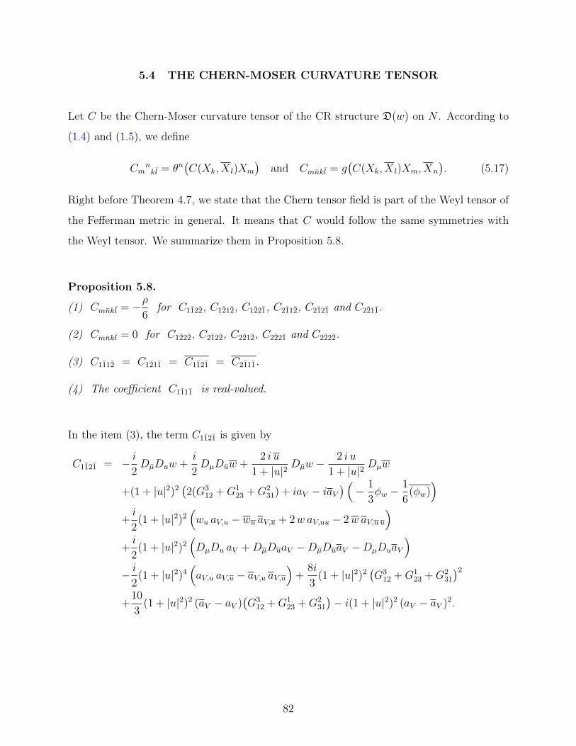
5.4 THE CHERN-MOSER CURVATURE TENSOR
Let C be the Chern-Moser curvature tensor of the CR structure D(w) on N . According to
(1.4) and (1.5), we define
Cmnkl = θn
(C(Xk, X l)Xm
)and Cmnkl = g
(C(Xk, X l)Xm, Xn
). (5.17)
Right before Theorem 4.7, we state that the Chern tensor field is part of the Weyl tensor of
the Fefferman metric in general. It means that C would follow the same symmetries with
the Weyl tensor. We summarize them in Proposition 5.8.
Proposition 5.8.
(1) Cmnkl = −ρ6
for C1122, C1212, C1221, C2112, C2121 and C2211.
(2) Cmnkl = 0 for C1222, C2122, C2212, C2221 and C2222.
(3) C1112 = C1211 = C1121 = C2111.
(4) The coefficient C1111 is real-valued.
In the item (3), the term C1121 is given by
C1121 = − i2DµDuw +
i
2DµDuw +
2 i u
1 + |u|2Dµw −
2 i u
1 + |u|2Dµw
+(1 + |u|2)2(2(G3
12 +G123 +G2
31) + iaV − iaV) (− 1
3φw −
1
6(φw)
)+i
2(1 + |u|2)2
(wu aV,u − wu aV,u + 2w aV,uu − 2w aV,u u
)+i
2(1 + |u|2)2
(DµDu aV +DµDuaV −DµDuaV −DµDuaV
)− i
2(1 + |u|2)4
(aV,u aV,u − aV,u aV,u
)+
8i
3(1 + |u|2)2
(G3
12 +G123 +G2
31
)2
+10
3(1 + |u|2)2 (aV − aV )
(G3
12 +G123 +G2
31
)− i(1 + |u|2)2 (aV − aV )2.
82

In the item (4), before the result ‘C = W ’ is proven, it is not obvious that C1111 is real-
valued. We may justify this fact directly. In the following, we let θ = G312 + G1
23 + G231 and
y = 1 + |u|2. C1111 can be broken down to two terms:
C1111 = Term1 + Term2.
Term1 contains all terms involving w and its derivatives, and Term2 contains the rest.
Term1 = −i(DµDµw + wuDµw + 2wD v
|v|w +
4uw
yDµw
)+i(DµDµw + wuDµw + 2wD v
|v|w +
4uw
yDµw
)+iy2
6
(2θ + iaV − iaV
)2(φw − (φw)
)−y2
(2θ + iaV − iaV
)(DµDuw +DµDuw
)+iy2
[Dµw
(4aV,u − aV,u
)−Dµw
(4aV,u − aV,u
)]+4y
(2θ + iaV − iaV
)(uDµw + uDµw − uwwu − uwwu + 4|w|2
)+y2
(2θ + iaV − iaV
)|wu|2
+iy2[− wwu
(aV,u − 2aV,u
)+ wwu
(aV,u − 2aV,u
)]−y2
[wu
(2Dµθ + iDµaV − iDµaV
)+ wu
(2Dµθ + iDµaV − iDµaV
)]+y4
(2θ + iaV − iaV
)(2wu aV,u + w aV,uu + 2wu aV,u + w aV,u u
)+y |w|2
(8i u aV,u − 8i u aV,u + 4i u aV,u − 4i u aV,u
)+iy2
[w(2DµDuaV −DµDuaV
)− w
(2DµDuaV −DµDuaV
)]+y[4uw
(2Dµθ + iDµaV − iDµaV
)+ 4uw
(2Dµθ + iDµaV − iDµaV
)]−y3
(2θ + iaV − iaV
)(6uw aV,u + 6uw aV,u
)+2iy4
[w(aV,u aV,u − 2
(aV,u
)2)− w
(aV,u aV,u − 2
(aV,u
)2)]
−|w|2(
40θ + 24iaV − 24iaV
)
83
Term1 is real-valued by observation. Moreover, we have
Term2 = (1 + |u|2)2(
2DµDµθ + iDµDµaV − iDµDµaV
)−(1 + |u|2)4
(2θ + iaV − iaV
)(4iD v
|v|θ +DµDuaV − 2D v
|v|aV
)−(1 + |u|2)4
(4(Dµθ) aV,u + 2(Dµθ) aV,u
)−i(1 + |u|2)4
[(2DµaV −DµaV
)aV,u −
(2DµaV −DµaV
)aV,u
]+(1 + |u|2)6
(2θ + iaV − iaV
)(aV,u aV,u + aV,u aV,u
)
+(1 + |u|2)4
−16
3θ3 − 8i
3θ2(5aV − 2aV
)+
4
3θ(7aV − aV
)(aV − aV
)+ 2iaV
(aV − aV
)2
.Term2 can be divided into three parts, each of them being a real component. The first
component is called σ1.
σ1 = y2(iDµDµaV − iDµDµaV
)− y4
(2 (Dµθ) aV,u + 2 (Dµθ) aV,u
)−iy4
[(2DµaV −DµaV
)aV,u −
(2DµaV −DµaV
)aV,u
]+y6
(2θ + iaV − iaV
)aV,u aV,u
+y4(− 16
3θ3 − 16i
3θ2(aV − aV
)+
4
3θ(aV − aV
)2).
σ1 is naturally a real-valued term. Next, we let
σ2 =(2θ + iaV − iaV
)(y6 aV,u aV,u − y4
(2iD v
|v|θ +DµDuaV − 2D v
|v|aV))
+y4(− 8i θ2 aV + 8 θ aV (aV − aV ) + 2i aV
(aV − aV
)2),
σ3 = 2y2 (DµDµθ)− y4(2θ + iaV − iaV
)(2iD v
|v|θ)− 2y4 (Dµθ) aV,u.
.
The last part of σ2 can be simplified as
−8i θ2 aV + 8 θ aV (aV − aV ) + 2i aV(aV − aV
)2
= (2θ + iaV − iaV )(− 2a2
V − 4i θ aV)− 8i θ2 (aV − aV ) + 8 θ (a2
V + a2V )− 12 θ |aV |2
+2i (aV − aV )(a2V + a2
V − |aV |2).
84

So, we have
σ2 = y4(2θ + iaV − iaV )(y2 aV,u aV,u −DµDuaV + 2D v
|v|aV − 2iD v
|v|θ − 2a2
V − 4iθ aV
)+y4
(− 8iθ2(aV − aV ) + 8θ(a2
V + a2V )− 12θ |aV |2 + 2i(aV − aV )
(a2V + a2
V − |aV |2)).
We may show that the expression
DµDuaV − y2 aV,u aV,u − 2D v|v|aV + 2iD v
|v|θ + 4i θ aV + 2a2
V (5.18)
is of real values later in this chapter. So σ2 is real-valued. We then consider the term σ3 in
the way that
σ3 = Re(2y2DµDµθ
)+ i Im
(2y2DµDµθ
)− 2i y4
(2θ + iaV − iaV
)D v
|v|θ − 2 y4 (Dµθ) aV,u.
The imaginary part of 2y2DµDµθ multiplied by i is:
i Im(2y2DµDµθ
)= y2
(DµDµθ −DµDµθ
)= y2 dθ
([µ, µ]
)= y2 dθ
(− aM µ+ aM µ− 2i h11
v
|v|
)= −y2 aM Dµθ + y2 aM Dµθ − 2i y2 h11D v
|v|θ
= y4 aV,uDµθ − y4 aV,uDµθ + 2i y4(2θ + iaV − iaV
)D v
|v|θ.
Therefore, σ3 = Re(2y2DµDµθ
)− y4
(aV,uDµθ + aV,uDµθ
), which is also of real values.
Our discussion above justifies that C1111 is real-valued.
85

5.5 FEFFERMAN METRIC IN THE GENERAL SETTING
Let F be the Fefferman metric of the CR structure D(w) on C(N). The connection forms
ω11 and ω2
2 of the Tanaka-Webster connection are given by:
ω11 = Γ1
11 θ1 + Γ1
11 θ1 + Γ1
21 θ2 + Γ1
01 α
=(wu −
2uw
1 + |u|2− 2T 4
)θ1 − aM θ1 +
( 2u
1 + |u|2)θ2 +
(− aV +
2uT 4
1 + |u|2)α;
ω22 = Γ2
12 θ1 + Γ2
22 θ2 + Γ2
12 θ1 + Γ2
02 α
= aM θ1 − 2u
1 + |u|2θ2 +
( 2uw
1 + |u|2+ 2T4 − wu
)θ1 − ∂T4
∂uα.
By (1.7), we have
F = 2h11 θ1 θ1 + 2 i θ2 θ1 − 2 i θ1 θ2 +
1
2α dγ
+
[− ρ
24+i
2
(− aV +
2uT 4
1 + |u|2− ∂T4
∂u
)]α α− i u
1 + |u|2α θ2 +
i u
1 + |u|2α θ2
+i
2
(wu −
2uw
1 + |u|2− 2T 4 + aM
)α θ1 − i
2
(wu −
2uw
1 + |u|2− 2T4 + aM
)α θ1.
The metric coefficients of F are then found by:
F (X1, X1) = h11
F (X1, X2) = −i
F (X1, T ) =i
4
(Γ1
11 + Γ212
)=
i
4
(wu −
2uw
1 + |u|2− 2T 4 + aM
)F (X2, T ) =
i
4Γ2
22 = − i u
2(1 + |u|2)
F (T, T ) = − ρ
24+i
2
(Γ1
01 + Γ202
)= − ρ
24+i
2
(− aV +
2uT 4
1 + |u|2− ∂T4
∂u
)F (T, ∂
∂γ) =
1
4
Similar to (4.9), we let u1 = X1, u2 = X1, u3 = X2, u4 = X2, u5 = T and u6 =∂
∂γ.
86
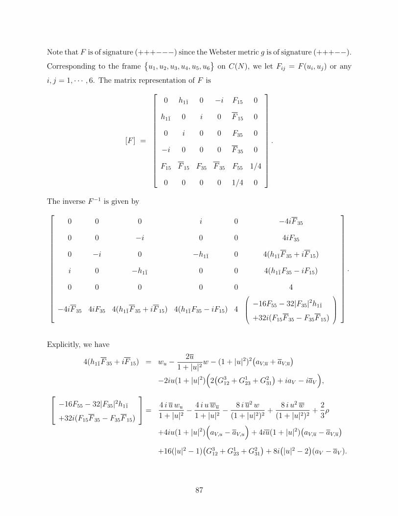
Note that F is of signature (+++−−−) since the Webster metric g is of signature (+++−−).
Corresponding to the frameu1, u2, u3, u4, u5, u6
on C(N), we let Fij = F (ui, uj) or any
i, j = 1, · · · , 6. The matrix representation of F is
[F ] =
0 h11 0 −i F15 0
h11 0 i 0 F 15 0
0 i 0 0 F35 0
−i 0 0 0 F 35 0
F15 F 15 F35 F 35 F55 1/4
0 0 0 0 1/4 0
.
The inverse F−1 is given by
0 0 0 i 0 −4iF 35
0 0 −i 0 0 4iF35
0 −i 0 −h11 0 4(h11F 35 + iF 15)
i 0 −h11 0 0 4(h11F35 − iF15)
0 0 0 0 0 4
−4iF 35 4iF35 4(h11F 35 + iF 15) 4(h11F35 − iF15) 4
−16F55 − 32|F35|2h11
+32i(F15F 35 − F35F 15)
.
Explicitly, we have
4(h11F 35 + iF 15) = wu −2u
1 + |u|2w − (1 + |u|2)2
(aV,u + aV,u
)−2iu(1 + |u|2)
(2(G3
12 +G123 +G2
31
)+ iaV − iaV
), −16F55 − 32|F35|2h11
+32i(F15F 35 − F35F 15)
=4 i uwu1 + |u|2
− 4 i uwu1 + |u|2
− 8 i u2w
(1 + |u|2)2+
8 i u2w
(1 + |u|2)2+
2
3ρ
+4iu(1 + |u|2)(aV,u − aV,u
)+ 4iu(1 + |u|2)
(aV,u − aV,u
)+16(|u|2 − 1)
(G3
12 +G123 +G2
31
)+ 8i
(|u|2 − 2
)(aV − aV ).
87

Let ∇ be the Levi-Civita connection of F and define ∇uiuj = Γkijuk. The Christoffel symbols
Γkij could be found by the Koszul formula (1.8). We also define R to be the Riemann tensor
of ∇ with
R(ui, uj)uk = Rlijk ul and Rijkl = F
(R(ui, uj)uk, ul
).
See (1.9) and (1.10). Moreover, Ric denotes the Ricci tensor of R with Rij (1.11), and S
denotes the scalar curvature of ∇ (1.12). The raise-index of Ric is Ric] (Rji = RikF
kj).
Let W be the Weyl curvature tensor of ∇ on C(N). From (1.15) and (1.16), we define
W(ui, uj)uk = W lijk ul and Wijkl = W
(ui, uj, uk, ul
)= F
(W(ui, uj)uk, ul
). (5.19)
The discussion of the Weyl tensor will be delayed to the next chapter. By Theorem 1.4
(J.M.Lee), the scalar curvature S can be found by
S =5
3ρ =
5i
3
(φw − (φw)
)− 5i
3
(φf − (φf )
). (5.20)
See Theorem 5.7. We mentioned before that the expression (5.18) is real-valued. Observe
that R12 = Ric(X1, X1), is real-valued by default. Using the notation θ = G312 + G1
23 + G231
and y = 1 + |u|2, we have
R12 =−1
2DµDuw −
1
2DµDuw +
2u
yDµw +
2u
yDµw −
iy2
12
(2θ + iaV − iaV
)(wuu − wuu
)+
1
4|wu|2 −
1
2y
(uwwu + uwwu
)+y2
4
(aV,u − aV,u
)wu +
y2
4
(aV,u − aV,u
)wu
+iy
2
(2θ + iaV − iaV
)(uwu − uwu
)− i(2θ + iaV − iaV
)(u2w − u2w
)+u y
(− 3
2aV,u +
1
2aV,u
)w + u y
(− 3
2aV,u +
1
2aV,u
)w +
y + 1
y2|w|2
+y4
4
(∣∣aV,u∣∣2 − 3∣∣aV,u∣∣2 − 3 aV,u aV,u + aV,u aV,u
)+y2
(1
2DµDuaV +
1
2DµDuaV +DµDuaV −D v
|v|aV +D v
|v|aV
)+y2
(2iD v
|v|θ − 20
3θ2 − 22i
3θ aV +
34i
3θ aV − 6|aV |2 + 2a2
V + 4a2V
)
88
R12 consists of a real term added by
−y4 aV,u aV,u + y2DµDuaV − 2 y2D v|v|aV + y2
(2iD v
|v|θ + 4i θ aV + 2a2
V
)= y2
(DµDuaV − y2 aV,u aV,u − 2D v
|v|aV + 2iD v
|v|θ + 4i θ aV + 2a2
V
),
which must be also a real term. Therefore, the expression (5.18) is real.
89

6.0 WEYL CURVATURE TENSOR (I)
Based on the local model of D(w) in (5.5), we are going to analyze the Weyl curvature tensor
of the Fefferman metric on C(N). As a remark, the CR distribution D(w) is spanned by
X2 =∂
∂uand
X1 = (u2 − 1) e1 + 2u e2 + i(u2 + 1) e3 + w(x, u)∂
∂u
at (x, u) on N . The associated contact form of D(w) is chosen as α in (5.6).
6.1 PROPERTIES OF THE WEYL TENSOR
The Weyl tensor (5.19) obeys the symmetries that
W[ij]kl =Wij[kl] = 0, Wijkl =Wklij, W[ijk]l =1
3
(Wijkl +Wjkil +Wkijl
)= 0.
By first two symmetries, we have 120 components of Wijkl’s in the collectionWijkl | i < j, k < l, i ≤ k and j ≤ l
.
These coefficients are divided into different categories according to their properties.
Class 1: Wijkl’s with at least one of i ,j, k, l being ‘6’
The is a number of 65 Wijkl’s with one or more of the indices being ‘6’. The Sparling
condition [6] [18] implies that ι ∂∂γW = 0 and so these coefficients are zero.
90

Theorem 6.1. W(∂∂γ, Z1, Z2, Z3
)= 0 for any tangent vectors Z1, Z2 and Z3 on C(N).
Class 2: Wijkl’s evaluated on the Levi distribution
We consider the values of W on D(w) ⊕D(w) in Class 2. In other words, all i, j, k and l
are from 1, 2, 3, 4. There are 21 components of Wijkl’s in this class:
W1212, W1213, W1214, W1223, W1224, W1234, W1313, W1314, W1323, W1324, W1334,
W1414, W1423, W1424, W1434, W2323, W2324, W2334, W2424, W2434, W3434.
As a general fact, the coefficients in Class 2 coincide with that of the Chern curvature tensor
in equation (5.17).
Theorem 6.2. For the CR structure D(w) on N , let C be the Chern curvature tensor (5.17)
associated with the contact form α. Also let F be the Fefferman metric associated with α on
C(N) and W (5.19) be its Weyl tensor. Then,
(1) : Cmnkl =W(Xm, Xn, Xk, X l) for every m, n, k, l.
(2) : W(Xm, Xn, Z1, Z2) = 0 for any Z1, Z2 are tangent vectors on C(N).
We include a proof of Theorem 6.2 in the Appendix B. The assertion (1) implies
W1212 = C1111, W1214 = C1112, W1223 = −C1121, W1234 = C1122, W1414 = C1212.
W1423 = −C1221, W1434 = C1222, W2323 = C2121, W2334 = −C2122, W3434 = C2222.
The above terms can be found by Proposition 5.8. Moreover, we have
W1213 =W1224 =W1313 =W1314 =W1323 =W1324 = 0,
W1334 =W1424 =W2324 =W2424 =W2434 = 0.
91

Class 3: Other coefficients of the form W13kl, W24kl, Wij13 or Wij24.
We may use the assertion (2) of Theorem 6.2 to show that these coefficients are zero. They
include: W1315, W1325, W1335, W1345, W1524, W2425, W2435, W2445.
6.2 COMPONENTS OF THE WEYL TENSOR INVOLVING T
Class 4: Wijkl’s related to the scalar curvature ρ
The components of Wijkl’s in Class 4 contain two indices selected from ‘3’ or ‘4’, and the
other two from ‘1’, ‘2’, or ‘5’. They include
W1435, W1445, W1534, W2335, W2345, W2534, W3535, W3545, W4545.
All of these terms could be expressed by the scalar curvature ρ and its u- or u-derivatives.
If ρ vanishes, then every one of them vanishes.
Proposition 6.3. Referring to the model (5.5) of D(w), we have the following.
(1) W1435 = W1534 = −W2335 = − 1
24
∂ρ
∂u
(2) W1445 = −W2345 = W2534 =1
24
∂ρ
∂u
(3) W3535 = − 1
48
∂2ρ
∂u2− u
24(1 + |u|2)
∂ρ
∂u
(4) W3545 = − ρ
24(1 + |u|2)2
(5) W4545 = − 1
48
∂2ρ
∂u2 −u
24(1 + |u|2)
∂ρ
∂u
We include formulas for ρ, ρu and ρuu here. Write θ = G312 +G1
23 +G231 and y = 1 + |u|2.
92

ρ = i(φw − (φw)
)+ 16 θ + 12i aV − 12i aV
ρu = i wuuu −6iu
ywuu +
18iu2
y2wu −
24 i u3
y3w +
6i
y2wu −
24 i u
y3w + 12i aV,u − 12i aV,u
ρuu = i wuuuu −6 i u
ywuuu +
24 i u2
y2wuu −
60 i u3
y3wu +
72 i u4
y4w
−12 i u
y3wu +
72 i |u|2
y4w − 24i
y3w + 24i aV,uu +
24 i u
y
(aV,u + aV,u
)As a remark, in our computation, we find that
W3435 = W3445 = 0.
We would put these two terms to Class 4 for convenience.
Class 5: The coefficients of Wijkl’s almost linear in w
There are 15 (out of 120) coefficients of the Weyl tensor left on our list. If we collect the
values of
W(X1, X1, η1, η2
), W
(X1, T, η1, η2
)and W
(X1, T, η1, η2
),
where the pair of vectors (η1, η2) is either (X1, X2), (X1, X2), (X2, T ) or (X2, T ), then we
obtain the Class 5 of 10 Weyl tensor coefficients:
W1235, W1245, W1415, W1425, W1523, W1535, W1545, W2325, W2535, W2545.
We may apply the symmetries of W to these 10 terms. First of all, W1235 = −W1245. By
the identity W1jk5Fjk = 0,
W1145F14 +W1235F
23 +W1325F32 +W1415F
41 = 0.
It leads toW1415 =W1235. Using the Bianchi identity toW1245, we also haveW1425 =W1245.
In summary, we have
W1235 = −W1245 = W1415 = W2325 = −W1425 = −W1523.
93

Moreover, W1535 =W2545 and W1545 =W2535. Therefore, it suffices to studyW1235,W1535
and W1545. We may also put W1214 (or W1223) to this category of Wijkl’s since it shares the
main properties with the above 10 coefficients.
Proposition 6.4.
Assume w = f , where f is defined by (5.4), and so the CR structure D(w) is of zero torsion.
Then, W1214 =W1235 =W1535 =W1545 = 0.
In Proposition 5.8, we include an explicit formula for C1121, which is as same as W1214.
Proposition 6.4 helps us rewrite W1214 as
W1214 = − i2DµDu(w − f) +
i
2DµDu(w − f) +
2 i u
yDµ(w − f)− 2 i u
yDµ(w − f)
+y2(2 θ + i aV − i aV
) (− 1
3φw −
1
6(φw) +
1
3φf +
1
6(φf )
)+iy2
2
((wu − fu) aV,u − (wu − fu) aV,u + 2(w − f) aV,uu − 2(w − f) aV,u u
)We include the results for W1235, W1535 and W1545 here.
W1235 =1
24w ρu −
i
12DµDuDu(w − f)− i
24DµDuDu(w − f) +
i
4D v
|v|Du(w − f)
−y2
24
(2 θ + i aV − i aV
)(wuuu − fuuu) +
iu
4yDµDu(w − f) +
iu
2yDµDu(w − f)
−iuyD v
|v|(w − f) +
iy2
8(wuu − fuu) aV,u +
u y
4
(2 θ + i aV − i aV
)(wuu − fuu)
− i
2y2Dµ(w − f)− iu2
2y2Dµ(w − f)− iu2
y2Dµ(w − f)
+(3 i y2
8aV,uu +
3 i u y
4aV,u −
3u2
4
(2 θ + i aV − i aV
))(wu − fu)
+(1
2θ +
i
4aV −
3 i u y
4aV,u
)(wu − fu)
+(u3
y
(2 θ + i aV − i aV
)− 3 i u y
2aV,uu − 3i u2 aV,u
)(w − f)
+(3 i u2
2aV,u + i aV,u −
i
2aV,u −
u
y
(2 θ + i aV
))(w − f)
94

W1535 =− 1
12y2w ρ− i
48DµDuDuDu(w − f) +
iu
8yDµDuDu(w − f)− iy2
48(wuuu − fuuu)aV,u
−3i u2
8y2DµDu(w − f) +
i
8y2DµDu(w − f) +
(5i y2
48aV,uu +
i u y
3aV,u
)(wuu − fuu)
+(iy2
48aV,uu +
i u y
24aV,u
)(wuu − fuu) +
iu3
2y3Dµ(w − f)− iu
2y3Dµ(w − f)
− i
y2D v
|v|(w − f)−
(5i u y
8aV,uu +
13i u2
8aV,u
)(wu − fu)
+(3i
8aV,u −
i
2aV,u −
i u y
8aV,uu −
iy
4aV,u
)(wu − fu)
+(5i u2
4aV,uu +
3i u3
yaV,u
)(w − f)
+(iu2
4aV,uu +
iu
2aV,u −
iu
yaV,u +
2i u
yaV,u +
1
y2
(θ + i aV − 2i aV
))(w − f)
W1545 =− 1
96
(w ρuu+w ρuu
)− 1
96
(wu−
2u
yw)ρu −
1
96
(wu−
2u
yw)ρu +
ρ
192
(φw+(φw)
)− i
96DµDuDuDu(w − f) +
i
96DµDuDuDu(w − f) +
iu
16yDµDuDu(w − f)
− iu
16yDµDuDu(w − f) +
i
24D v
|v|DuDu(w − f)− i
24D v
|v|DuDu(w − f)
+iy2
32aV,u(wuuu − fuuu)−
iy2
32aV,u(wuuu − fuuu)
−( θ
12+
i
16aV −
i
16aV
)(φw + (φw)− φf − (φf )
)+i
4y
(uD v
|v|Du(w−f)− uD v
|v|Du(w−f)
)+
i
16y2
(DµDu(w−f)−DµDu(w−f)
)+
3i
16y2
(u2DµDu(w − f)− u2DµDu(w − f)
)+(iaV
24− 3i u y
16aV,u
)(wuu − fuu)
+(3i u y
16aV,u −
iaV24− θ
12
)(wuu − fuu) +
iu2
2y2D v
|v|(w − f)− iu2
2y2D v
|v|(w − f)
+i
4y3
(uDµ(w − f)− uDµ(w − f) + u3Dµ(w − f)− u3Dµ(w − f)
)+( i
8aV,u −
3i
16aV,u +
9i u2
16aV,u −
i u aV4y
)(wu − fu)
+( 3i
16aV,u −
i
8aV,u −
9i u2
16aV,u +
u
4y
(2θ + iaV
))(wu − fu)
+( i
8aV,uu −
i
8aV,uu −
iu
4yaV,u +
iu
2yaV,u −
3i u3
4yaV,u +
i u2 aV2y2
)(w − f)
+( i
8aV,u u −
i
8aV,u u +
3i u3
4yaV,u −
iu
2yaV,u +
iu
4yaV,u −
u2
2y2
(2θ + iaV
))(w − f)
95

By observation, as long as ρ = 0, W1214, W1235, W1535 and W1545 would be linear in w,
its derivatives and their respective complex conjugations over the ring of complex-valued
functions in u, Gkij’s and Gk
ij,m’s. In other words, should ρ = 0, these four terms would be in
the form of
∑k
(akD
kuw + bkDµ(Dk
uw) + ckDµ(Dkuw) + dkD v
|v|(Dk
uw)
+ akDkuw + bkDµ(Dk
uw) + ckDµ(Dkuw) + dkD v
|v|(Dk
uw)) (6.1)
Here Dkuw is the k-th order u-derivative of w. ak, bk, ck, dk and other coefficients are complex-
valued functions in u, Gkij’s and Gk
ij,m’s. As a remark, we say that the coefficients in Class 5
are almost linear in w because they all satisfy the property (6.1).
Proposition 6.5.
Under the assumption that ρ = 0, the following coefficients of the Weyl tensor,
W1214, W1223, W1235, W1245, W1415, W1425, W1523, W1535, W1545, W2325, W2535, W2545,
are linear in w, its derivatives and their respective complex conjugations over the ring of
complex-valued functions in u, Gkij’s and Gk
ij,m’s.
96
6.3 THE TWISTOR CR MANIFOLD OF ZERO TORSION
The Class 6 of coefficients of the Weyl tensor consists of the remaining terms. Combining
W1212 to them, we have the terms
W1212, W1215, W1225, W1515, W1525 and W2525.
By complex conjugation, it suffices to consider W1212, W1215, W1515 and W1525.
They are the most complicated components in the Weyl tensor since they involve the second
derivatives of Gkij’s on the 3-manifold M . Much work is still required to study these terms
in the general case. However, when the CR structure is of zero torsion (w = f), we would
understand them fully by the Schouten tensor P (and hence the Cotton tensor) on M .
From our notation in Chapter 2, e1, e2, e3 is an orthonormal frame on M . ∇M represents
the Riemannian connection of the metric g on M . Let Gkij = g
(∇Meiej, ek
)be the Christoffel
symbols. We then denote the Riemann tensor on M by RM .
Rijkl = g(RM(ei, ej)ek, el
).
The Ricci tensor is named by RicM with Rij = RicM(ei, ej). Also we set the scalar curvature
to be R. The Schouten tensor P in 3-dimension is a symmetric (0,2) tensor such that
P = RicM −R
4g with Pij = P(ei, ej) = Rij −
R
4gij. (6.2)
If we write ∇iPjk = (∇MeiP)(ej, ek), then
∇iPjk = ei(Rjk)−ei(R)
4δjk −Gm
ij Pmk −Gmik Pmj. (6.3)
It is a fact that in three dimension, the metric g is conformally flat if and only if the Schouten
tensor is a Codazzi tensor: (∇MeiP)(ej, ek) = (∇M
ejP)(ei, ek) for every i, j, k = 1, 2, 3.
97
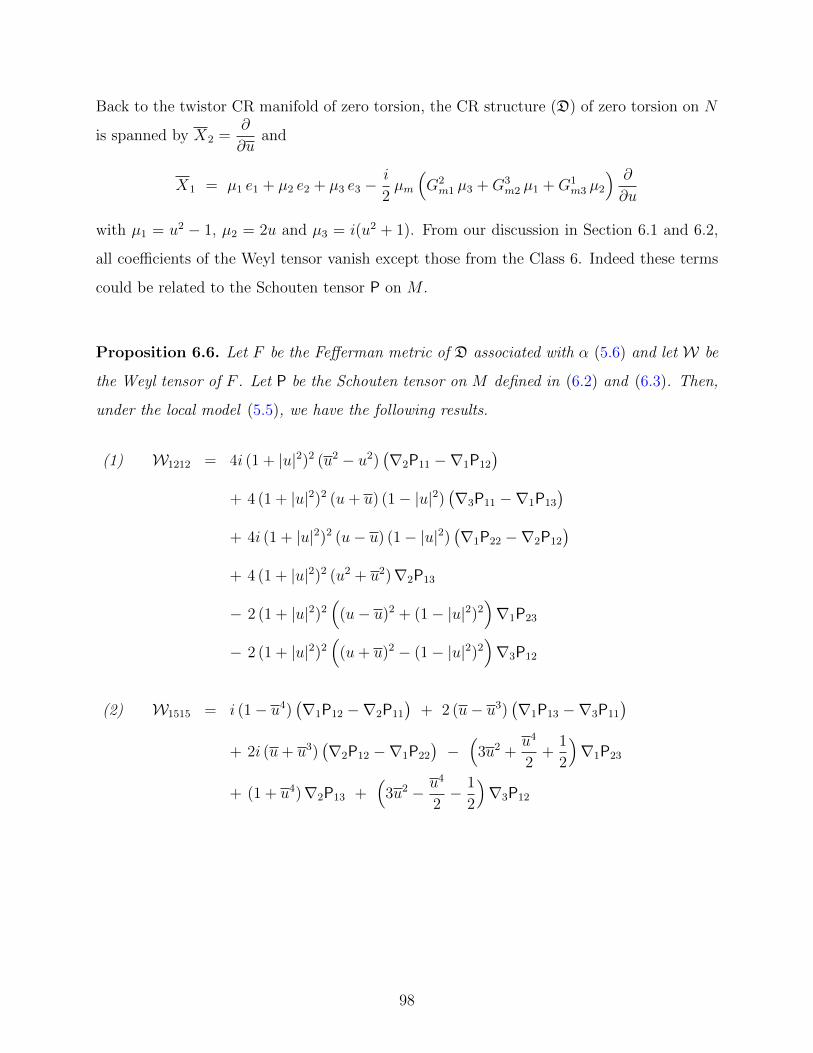
Back to the twistor CR manifold of zero torsion, the CR structure (D) of zero torsion on N
is spanned by X2 =∂
∂uand
X1 = µ1 e1 + µ2 e2 + µ3 e3 −i
2µm
(G2m1 µ3 +G3
m2 µ1 +G1m3 µ2
) ∂
∂u
with µ1 = u2 − 1, µ2 = 2u and µ3 = i(u2 + 1). From our discussion in Section 6.1 and 6.2,
all coefficients of the Weyl tensor vanish except those from the Class 6. Indeed these terms
could be related to the Schouten tensor P on M .
Proposition 6.6. Let F be the Fefferman metric of D associated with α (5.6) and let W be
the Weyl tensor of F . Let P be the Schouten tensor on M defined in (6.2) and (6.3). Then,
under the local model (5.5), we have the following results.
(1) W1212 = 4i (1 + |u|2)2 (u2 − u2)(∇2P11 −∇1P12
)+ 4 (1 + |u|2)2 (u+ u) (1− |u|2)
(∇3P11 −∇1P13
)+ 4i (1 + |u|2)2 (u− u) (1− |u|2)
(∇1P22 −∇2P12
)+ 4 (1 + |u|2)2 (u2 + u2)∇2P13
− 2 (1 + |u|2)2(
(u− u)2 + (1− |u|2)2)∇1P23
− 2 (1 + |u|2)2(
(u+ u)2 − (1− |u|2)2)∇3P12
(2) W1515 = i (1− u4)(∇1P12 −∇2P11
)+ 2 (u− u3)
(∇1P13 −∇3P11
)+ 2i (u+ u3)
(∇2P12 −∇1P22
)−(
3u2 +u4
2+
1
2
)∇1P23
+ (1 + u4)∇2P13 +(
3u2 − u4
2− 1
2
)∇3P12
98

(3) W1215 = 2i (1 + |u|2) (u+ u3)(∇1P12 −∇2P11
)+ i (1 + |u|2)
(uu3 − 3u2 + 3|u|2 − 1
) (∇2P12 −∇1P22
)+ (1 + |u|2)
(uu3 − 3u2 − 3|u|2 + 1
) (∇3P11 −∇1P13
)− (1 + |u|2)
(u− 3u+ 3uu2 − u3
)∇1P23
+ 2 (1 + |u|2) (u− u3)∇2P13
− (1 + |u|2)(u+ 3u− 3uu2 − u3
)∇3P12
(4) W1525 = i (u2 − u2)(∇1P12 −∇2P11
)+(uu2 + u2 u− u− u
) (∇1P13 −∇3P11
)+ i
(uu2 − u2 u+ u− u
) (∇1P22 −∇2P12
)+
1
2
(4|u|2 − |u|4 − u2 − u2 − 1
)∇1P23 + (u2 + u2)∇2P13
+1
2
(|u|4 − 4|u|2 − u2 − u2 + 1
)∇3P12
Proposition 6.6 is justified by computer programming in Matlab. We replace the variable
aV and its derivatives by the Christoffel symbols Gkij and their derivatives. In the process,
the second derivatives, Gkij,pl = el ep
(Gkij
), can be substituted with ∇iPjk’s. So we get the
formulas regarding W1212, W1515, W1215 and W1525. A detailed explanation regarding the
computational model is included in Appendix C.
Theorem 6.7. Let M be a 3-manifold equipped with the metric g, and let (N,D) be the
twistor CR manifold of (M, g). Let F be the Fefferman metric of D associated with any
contact form θ on N . Then, g is conformally flat if and only if F is conformally flat (which
is equivalent to the vanishing of the Weyl tensor).
99

Proof. If g is conformally flat, then Theorem 7.3 implies that w = 0 is a sufficient condition
for the Weyl tensor to vanish. Therefore, F is conformally flat. On the other hand, if we
assume that the Weyl tensor is zero, then it suffices to prove that the Cotton tensor of (M, g)
vanishes.
Let Cijk be the component of the Cotton tensor with Cijk = ∇kPij − ∇jPik. Note that
Cijk = −Cikj and Cijk + Cjki + Ckij = 0. Moreover, in 3 dimension, we have the result:
C121 = C332, C221 = C313, C131 = C223. (6.4)
Therefore, we obtain the following symmetries.
C112 = −C121 = −C332 = C323
C113 = −C131 = −C223 = C232
C212 = −C221 = −C313 = C331
C123 = −C132, C231 = −C213, C312 = −C321
C123 + C231 + C312 = 0
(6.5)
When W = 0, in particular, W1212 = 0. We could write
1
4(1 + |u|2)2W1212 =
(i u2 − i u2
)C112 +
(u+ u− uu2 − u2 u
)C113
+(i u− i u+ i u u2 − i u2 u
)C221
+1
2
(4|u|2 − |u|4 − 1− u2 − u2
)C321
+1
2
(|u|4 − 4|u|2 + 1− u2 − u2
)C123.
WhenW1212 = 0, by comparing the coefficients of |u|4, we get C321 = C123. Also, considering
the terms of u2 u, −C113 − iC221 = 0. So C221 = iC113. As a result,
(iu2 − iu2
)C112 +
(2u− 2uu2
)C113 −
(u2 + u2
)C123 = 0
Immediately, we have C113 = 0, iC112 − C123 = 0 and −iC112 − C123 = 0. Therefore,
C113 = C112 = C123 = 0.
100

7.0 WEYL CURVATURE TENSOR (II)
When M is equipped with the Euclidean metric, the model of the twistor CR structure (4.1)
becomes much simpler. So we can obtain specific results for the Weyl tensor of the Fefferman
metric. Especially, we may solve for non-trivial torsion function w such that the Weyl tensor
vanishes completely for D(w).
7.1 THE ALMOST w-LINEAR COMPONENTS
Suppose M is a flat 3-manifold and x = (x1, x2, x3) is the coordinate system on M . The CR
structure D(w) on the sphere bundle N (of M) is described byX1 = (u2 − 1)
∂
∂x1
+ 2u∂
∂x2
+ i(u2 + 1)∂
∂x3
+ w(x, u)∂
∂u
X2 =∂
∂u
See (4.1). Moreover, by Theorem 4.6, the scalar curvature S (or ρ) of the Fefferman metric
F is zero if and only if w is in the form of (4.12):
w = λ0 + λ1 u+K u2 − λ1 u3 + λ0 u
4.
λ0, λ1 are complex-valued functions on M , and K is a real-valued function on M .
From our discussion in Chapter 6, if w satisfies the condition (4.12), then all the coefficients
of the Weyl tensor would vanish except those from Class 5 and Class 6.
101

The remaining terms could be reduced to 8 terms:
W1214, W1235, W1535, W1545, (from Class 5)
W1212, W1215, W1515, W1525. (from Class 6)
We first compute for the Class 5 coefficients, which are linear in w when ρ = 0. Let
A =∂λ1
∂x3
− i∂λ1
∂x1
+∂λ1
∂x3
+ i∂λ1
∂x1
,
B =∂K
∂x3
+ i∂K
∂x1
+ 2i∂λ0
∂x1
− 2∂λ0
∂x3
+ i∂λ1
∂x2
,
C =∂λ1
∂x3
+ i∂λ1
∂x1
+ 4i∂λ0
∂x2
.
We then have the following results.
W1214 = −A2
(1− 4|u|2 + |u|4
)−(Bu+Bu
)(1− |u|2) +
(Cu2 + Cu2
)W1235 = − 1
1 + |u|2(u2
4
(|u|2 − 3
)B +
1
4
(1− 3|u|2
)B +
3u
4
(|u|2 − 1
)A+
u3
2C − u
2C)
W1535 =1
(1 + |u|2)2
(− 3u2
4A− u3
2B +
u
2B +
u4
4C +
1
4C)
W1545 = − 1
(1 + |u|2)2
(1
8
(|u|4 − 4|u|2 + 1
)A+ (1− |u|2)
(u4B +
u
4B)− 1
4
(u2C + u2C
))
Proposition 7.1.
W1214, W1235, W1535 and W1545 are zero if and only if λ0, λ1 and K satisfy both of the
following equalities.
(1)∂λ1
∂x3
− i∂λ1
∂x1
+∂λ1
∂x3
+ i∂λ1
∂x1
= 0
(2)∂K
∂x3
+ i∂K
∂x1
+ 2i∂λ0
∂x1
− 2∂λ0
∂x3
+ i∂λ1
∂x2
= 0
(3)∂λ1
∂x3
+ i∂λ1
∂x1
+ 4i∂λ0
∂x2
= 0
102

Define the complex variable p = x1 + ix3. The above equations could be translated to
(1)∂λ1
∂p=∂λ1
∂p, (2)
∂K
∂p+ 2
∂λ0
∂p+
1
2
∂λ1
∂x2
= 0, (3)∂λ1
∂p+ 2
∂λ0
∂x2
= 0. (7.1)
We let λ1 = αpx2 + i βpx2 for two real-valued functions α(p, p, x2) and β(p, p, x2). The
equation (1) holds whenever βppx2 = 0. It means that β is decomposed to β = f + f + g,
where f = f(p, p, x2) is a complex-valued function holomorphic in p, and g = g(p, p) is
real-valued. As a result, we have
λ1 = αpx2 + i βpx2 = αpx2 + i fpx2 . (7.2)
The equation (3) means that∂λ0
∂x2
= −1
2
∂λ1
∂p= −1
2αppx2 + i βppx2 . Integrating by x2,
λ0 = − 1
2(αpp + i βpp) + τpp(p, p), (7.3)
where τ is a complex-valued function depending on p and p only. Finally, (2) implies that
∂K
∂p= − 2
∂λ0
∂p− 1
2
∂λ1
∂x2
=(αppp + i βppp − 2 τppp
)− 1
2
(αpx2x2 + i βpx2x2
).
Integrating by p, we have
K =(αpp −
1
2αx2x2
)+ i(βpp −
1
2βx2x2
)− 2 τpp + h(p, p, x2). (7.4)
Here h(p, p, x2) is a complex-valued function such that hp = 0. Moreover, since K is real-
valued, we obtain the identitiesK = Re(K) = αpp −
1
2αx2x2 − (τpp + τ pp) +
1
2(h+ h)
Im(K) = βpp −1
2βx2x2 + i(τpp − τ pp)−
i
2(h− h) = 0.
(7.5)
from (7.4). Substituting f + f + g for β in the second equation of (7.5), we get
gpp −1
2
(fx2x2 + fx2x2
)+ i(τpp − τ pp
)− i
2(h− h) = 0 (7.6)
103

When we differentiate (7.6) by x2,
−1
2
(fx2x2x2 + fx2x2x2
)− i
2(hx2 − hx2) = 0
(fx2x2x2 − i hx2
)+(fx2x2x2
+ i hx2
)= 0.
Since fx2x2x2−i hx2 is holomorphic in p and fx2x2x2+i hx2 is antiholomorphic in p, fx2x2x2−i hx2
is then a function depending only on x2. Integrating it by x2,
fx2x2 − i h = r(x2) + s(p, p)
for two complex-valued functions r(x2) and s(p, p) with sp = 0. Moreover,
h(p, p, x2) = i(fx2x2
− r(x2)− s(p, p)),
h(p, p, x2) = i(− fx2x2 + r(x2) + s(p, p)
).
(7.7)
To solve for r and s, note that from (7.6)
gpp + i(τpp − τ pp
)− 1
2
(fx2x2 − i h
)− 1
2
(fx2x2
+ i h)
= 0
gpp + i(τpp − τ pp
)− 1
2
(r + r
)− 1
2
(s+ s
)= 0
gpp − 2 Im(τ)pp − 12
(s+ s
)= 1
2
(r + r
).
(7.8)
The LHS of (7.8) depends on p and p only, while the RHS depends on x2 only. Therefore,
there exists a constant C0 such that
1
2(r + r) = C0 = gpp − 2 Im(τ)pp −
1
2
(s+ s
). (7.9)
Accordingly, we may write
r(x2) = C0 + iρ(x2) (7.10)
for a real-valued function ρ. In addition, by (7.8),
(gpp − 2 Im(τ)pp
)pp
=(C0 +
1
2(s+ s)
)pp
= 0.
So gpp − 2 Im(τ)pp = θpp for a real-valued function θ(p, p) such that θppp p = 0.
104
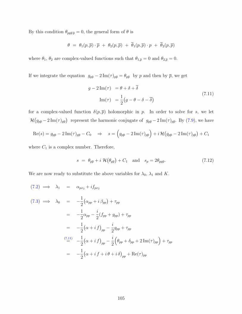
By this condition θppp p = 0, the general form of θ is
θ = θ1(p, p) · p + θ2(p, p) + θ1(p, p) · p + θ2(p, p)
where θ1, θ2 are complex-valued functions such that θ1,p = 0 and θ2,p = 0.
If we integrate the equation gpp − 2 Im(τ)pp = θpp by p and then by p, we get
g − 2 Im(τ) = θ + δ + δ
Im(τ) =1
2
(g − θ − δ − δ
) (7.11)
for a complex-valued function δ(p, p) holomorphic in p. In order to solve for s, we let
H(gpp− 2 Im(τ)pp
)represent the harmonic conjugate of gpp− 2 Im(τ)pp. By (7.9), we have
Re(s) = gpp − 2 Im(τ)pp − C0 ⇒ s =(gpp − 2 Im(τ)pp
)+ iH
(gpp − 2 Im(τ)pp
)+ C1
where C1 is a complex number. Therefore,
s = θpp + i H(θpp)
+ C1 and sp = 2θppp. (7.12)
We are now ready to substitute the above variables for λ0, λ1 and K.
(7.2) =⇒ λ1 = αpx2 + ifpx2
(7.3) =⇒ λ0 = −1
2
(αpp + i βpp
)+ τpp
= −1
2αpp −
i
2(fpp + gpp) + τpp
= −1
2
(α + i f
)pp− i
2gpp + τpp
(7.11)= −1
2
(α + i f
)pp− i
2
(θpp + δpp + 2 Im(τ)pp
)+ τpp
= −1
2
(α + i f + i θ + i δ
)pp
+ Re(τ)pp
105

(7.4) =⇒ K = αpp −1
2αx2x2 −
(τpp + τ pp
)+
1
2(h+ h)
(7.7)= αpp −
1
2αx2x2 − 2 Re(τ)pp +
i
2
(fx2x2
− r − s− fx2x2 + r + s)
= αpp −1
2αx2x2 −
i
2
(fx2x2 − fx2x2
)− 2 Re(τ)pp +
i
2
(r − r + s− s
)(7.10), (7.12)
= αpp −1
2αx2x2 −
i
2
(fx2x2 − fx2x2
)− 2 Re(τ)pp − ρ(x2)−H(θpp)
We could eliminate f , Re(τ) and δ by letting
α′ = α− 2 Re(τ) + i(f − f) and θ′ = θ + δ + δ.
First of all, we have α′px2= αpx2 + i fpx2 , so λ1 = α′px2
. Then, we note that
α′pp = αpp − 2 Re(τ)pp + i fpp and θ′pp = θpp + δpp.
Therefore, λ0 = −1
2
(α′ + i θ′
)pp
. Lastly, we have
α′pp −1
2α′x2x2
= αpp −1
2αx2x2 − 2 Re(τ)pp + i(f − f)pp −
i
2
(fx2x2 − fx2x2
)= αpp −
1
2αx2x2 −
i
2
(fx2x2 − fx2x2
)− 2 Re(τ)pp,
θ′pp = θpp + δpp + δpp = θpp.
Therefore, K = α′pp −1
2α′x2x2
− ρ(x2)−H(θ′pp).
We may also put θ′ = θ1 p+ θ2 + θ1 p+ θ2, then we get
θ′pp = θ1,pp p+ θ2,pp and H(θ′pp) = H(2 Re(θ1,p) = 2 Im(θ1,p) = −i(θ1,p − θ1,p).
By substitution,
λ0 = −1
2
(α′ + i θ′
)pp
= − 1
2α′ − i
2
(θ1,pp p+ θ2,pp
),
K = α′pp −1
2α′x2x2
− ρ(x2)−H(θ′pp) = α′pp −1
2α′x2x2
− ρ(x2) + i(θ1,p − θ1,p
).
106

Proposition 7.2. The general solution to the linear system of differential equations in
Proposition 7.1 (or (7.1)) is given by
λ1 = αpx2
λ0 = −1
2αpp −
i
2
(θ1,pp p+ θ2,pp
)K = αpp −
1
2αx2x2 − ρ(x2) + i
(θ1,p − θ1,p
)(7.13)
for arbitrary real-valued functions α(p, p, x2), ρ(x2), and complex-valued functions θ1(p, p),
θ2(p, p) which are holomorphic in p.
It is possible to further reduce the system (7.13) if we let
φ = α + i(θ1 p+ θ2 − θ1 p− θ2
)+R(x2).
Here R(x2) is a real-valued function such that Rx2x2 = 2ρ. (7.13) is then equivalent to,
λ1 = αpx2 = φpx2
λ0 = −1
2αpp −
i
2
(θ1,pp p+ θ2,pp
)= − 1
2φpp
K = αpp −1
2αx2x2 − ρ(x2) + i
(θ1,p − θ1,p
)= φpp −
1
2φx2x2
(7.14)
for an arbitrary real-valued functions φ(p, p, x2).
107

7.2 THE VANISHING OF THE WEYL TENSOR
In this section we will investigate under what kind of conditions on w, the Weyl tensor
vanishes completely. Suppose w = λ0 +λ1u+Ku2−λ1u3 +λ0u
4 satisfies (7.13). We would
discuss a very special case that the real-valued function α in (7.13) is in the form
α = x2(Ψ + Ψ). (7.15)
for a holomorphic function Ψ = Ψ(p). We also let ψ(p) = Ψ′(p).
(7.15) is a strict condition imposed on (7.13). It makes λ1 = ψ(p) be holomorphic in p
and eliminate the term αpp − (1/2)αx2x2 in the third equation. In the following, we also let
K0(x2) = −ρ(x2), θ1,p = ζ1 and θ2,pp = ζ2. Therefore, (7.13) becomes
λ1 = ψ(p)
λ0 = −x2
2ψ′(p)− i
2
(ζ ′1 p+ ζ2
)K = K0(x2) + i(ζ1 − ζ1)
(7.16)
where both ψ, ζ1 and ζ2 are holomorphic in p and independent of x2.
The Weyl tensor of D(w) vanishes if and only if W1212, W1215, W1515 and W1525 are all zero.
Both of these four coefficients of W are polynomials in u and u. More precisely,
W1212
(1 + |u|2)2= −F1(p, p)
(u2 u2 − 4uu+ 1
)−(F21 x
22 + F22 x2 + F23(p, p, x2)
)(u2 u− u)
−(F 21 x
22 + F 22 x2 + F 23(p, p, x2)
)(u2 u− u)
−(F31(p, p, x2)x2 + F32(p, p, x2)
)u2
−(F 31(p, p, x2)x2 + F 32(p, p, x2)
)u2.
108

The coefficient functions of W1212 are defined as follows.
F1 = ψ ζ′1 + ζ ′1 ψ +
1
2ψ′(ζ′1 p+ ζ2
)+
1
2ψ′(ζ ′1 p+ ζ2
)F21 = i ψ′ ψ
′′
F22 = ψ′(ζ′′1 p+ ζ
′2
)− ψ′′
(ζ ′1 p+ ζ2
)− ζ ′1 ψ
′
F23 = −2 ζ′1
(K0(x2) + i(ζ1 − ζ1)
)+ i(ζ′′1 p+ ζ
′2
)(ζ ′1 p+ ζ2
)+ iζ ′1
(ζ′1 p+ ζ2
)F31 = i
(ψ ψ
′′ −K ′0(x2)ψ′)
F32 = −K ′0(x2)(ζ′1 p+ ζ2
)− i ψ′
(K0(x2) + i(ζ1 − ζ1)
)+ ψ
(ζ′′1 p+ ζ
′2
)− ψ ζ ′1
In terms of F1, F21, F22, F23, F31 and F32, we also get other coefficients.
W1215
1 + |u|2= −3
2F1(uu2 − u)− 1
4
(F21 x
22 + F22 x2 + F23
)(3uu− 1)
−1
4
(F 21 x
22 + F 22 x2 + F 23
)(3u2 − uu3)− 1
2
(F31 x2 + F32
)u
+1
2
(F 31 x2 + F 32
)u3
W1515 = −3
2F1 u
2 − 1
2
(F21 x
22 + F22 x2 + F23
)u+
1
2
(F 21 x
22 + F 22 x2 + F 23
)u3
−1
4
(F31 x2 + F32
)− 1
4
(F 31 x2 + F 32
)u4
W1525 = −1
4F1
(u2 u2 − 4uu+ 1
)− 1
4
(F21 x
22 + F22 x2 + F23
)(u2 u− u)
−1
4
(F 21 x
22 + F 22 x2 + F 23
)(uu2 − u)− 1
4
(F31 x2 + F32
)u2
−1
4
(F 31 x2 + F 32
)u2
Therefore, the Weyl tensor vanishes if and only ifF1(p, p) = 0,
F21 x22 + F22 x2 + F23(p, p, x2) = 0,
F31(p, p, x2)x2 + F32(p, p, x2) = 0.
109
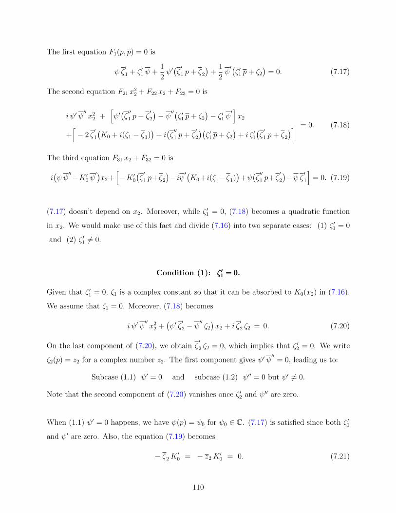
The first equation F1(p, p) = 0 is
ψ ζ′1 + ζ ′1 ψ +
1
2ψ′(ζ′1 p+ ζ2
)+
1
2ψ′(ζ ′1 p+ ζ2
)= 0. (7.17)
The second equation F21 x22 + F22 x2 + F23 = 0 is
i ψ′ ψ′′x2
2 +[ψ′(ζ′′1 p+ ζ
′2
)− ψ′′
(ζ ′1 p+ ζ2
)− ζ ′1 ψ
′]x2
+[− 2 ζ
′1
(K0 + i(ζ1 − ζ1)
)+ i(ζ′′1 p+ ζ
′2
)(ζ ′1 p+ ζ2
)+ i ζ ′1
(ζ′1 p+ ζ2
)] = 0. (7.18)
The third equation F31 x2 + F32 = 0 is
i(ψ ψ
′′−K ′0 ψ′)x2 +
[−K ′0
(ζ′1 p+ζ2
)−iψ′
(K0 +i(ζ1−ζ1)
)+ψ(ζ′′1 p+ζ
′2
)−ψ ζ ′1
]= 0. (7.19)
(7.17) doesn’t depend on x2. Moreover, while ζ ′1 = 0, (7.18) becomes a quadratic function
in x2. We would make use of this fact and divide (7.16) into two separate cases: (1) ζ ′1 = 0
and (2) ζ ′1 6= 0.
Condition (1): ζ ′1 = 0ζ ′1 = 0ζ ′1 = 0.
Given that ζ ′1 = 0, ζ1 is a complex constant so that it can be absorbed to K0(x2) in (7.16).
We assume that ζ1 = 0. Moreover, (7.18) becomes
i ψ′ ψ′′x2
2 +(ψ′ ζ
′2 − ψ
′′ζ2
)x2 + i ζ
′2 ζ2 = 0. (7.20)
On the last component of (7.20), we obtain ζ′2 ζ2 = 0, which implies that ζ ′2 = 0. We write
ζ2(p) = z2 for a complex number z2. The first component gives ψ′ ψ′′
= 0, leading us to:
Subcase (1.1) ψ′ = 0 and subcase (1.2) ψ′′ = 0 but ψ′ 6= 0.
Note that the second component of (7.20) vanishes once ζ ′2 and ψ′′ are zero.
When (1.1) ψ′ = 0 happens, we have ψ(p) = ψ0 for ψ0 ∈ C. (7.17) is satisfied since both ζ ′1
and ψ′ are zero. Also, the equation (7.19) becomes
− ζ2K′0 = − z2K
′0 = 0. (7.21)
110

If z2 = 0 in (7.21), we don’t have any restriction on K ′0(x2), so the Weyl tensor is zero when
(1.11)
λ1 = ψ(p) = ψ0
λ0 = −x2
2ψ′(p)− i
2
(ζ ′1 p+ ζ2
)= 0
K = K0(x2) + i(ζ1 − ζ1) = K0(x2)
for an arbitrary real-valued function K0(x2) and a complex constant ψ0.
On the other hand, if z2 6= 0 in (7.21), we require that K ′0(x2) = 0. Therefore,W is zero when
(1.12)
λ1 = ψ(p) = ψ0
λ0 = −x2
2ψ′(p)− i
2
(ζ ′1 p+ ζ2
)= −i z2
2
K = K0(x2) + i(ζ1 − ζ1) = K0
for arbitrary complex constants ψ0, z2 and a real constant K0.
When (1.2) ψ′′ = 0 but ψ′ 6= 0 happens, we let ψ(p) = α1 p+α2 with α1 6= 0. (7.17) becomes
1
2ψ′ ζ2 +
1
2ψ′ζ2 = 0 =⇒ α1 z2 + α1 z2 = 0. (7.22)
Moreover, (7.19) implies that:(− iK ′0 ψ
′)x2 +
(−K ′0 ζ2 − i ψ
′K0
)= 0
−i α1K′0 x2 − z2K
′0 − i α1K0 = 0.
(7.23)
If z2 = 0 in (7.22), then we don’t have any restriction on α1. In addition, x2K′0 + K0 = 0
from (7.23). So K0(x) =b
x2
for a real constant b. Hence, the Weyl tensor vanishes when
(1.21)
λ1 = ψ(p) = α1 p+ α2
λ0 = −x2
2ψ′(p)− i
2
(ζ ′1 p+ ζ2
)= −α1
2x2
K = K0(x2) + i(ζ1 − ζ1) =b
x2
for arbitrary complex numbers α1(6= 0), α2 and a real number b.
111

Suppose z2 6= 0 in (7.22). (7.22) becomes z2 = r · i α1 for some r ∈ R and r 6= 0.
−i α1K′0 x2 − z2K
′0 − i α1K0 = 0
−i α1K′0 x2 + i r α1K
′0 − i α1K0 = 0
K ′0 x2 − r K ′0 +K0 = 0
(x2 − r)K ′0 +K0 = 0
K ′0K0
= − 1
x2 − r
K0(x2) =b
x2 − r
for two real numbers b and r. Therefore, the Weyl tensor is zero when
(1.22)
λ1 = ψ(p) = α1 p+ α2
λ0 = −x2
2ψ′(p)− i
2
(ζ ′1 p+ ζ2
)= −α1
2(x2 − r)
K = K0(x2) + i(ζ1 − ζ1) =b
x2 − r
whenever α1(6= 0), α2 ∈ C and r, b ∈ R with r 6= 0.
Note that the solution (1.21) is a special case (r = 0) for the solution (1.22). The solution
sets in (1.11), (1.12) and (1.22) provide us with all choices of λ1, λ0 and K such that W is
zero when ζ ′1 = 0.
112

Condition (2): ζ ′1 6= 0ζ ′1 6= 0ζ ′1 6= 0.
We differentiate (7.18) and (7.19) by x2. The first derivative of (7.18) by x2 is
2i ψ′ ψ′′x2 +
[ψ′(ζ′′1 p+ ζ
′2
)− ψ′′
(ζ ′1 p+ ζ2
)− ζ ′1 ψ
′]− 2 ζ
′1K
′0 = 0. (7.24)
The second derivative of (7.18) by x2 is
2i ψ′ ψ′′ − 2 ζ
′1K
′′0 = 0. (7.25)
The first derivative of (7.19) by x2 is
i ψ ψ′′ − i ψ′K ′0 − i ψ
′K ′′0 x2 − (ζ
′1 p+ ζ2)K ′′0 − i ψ
′K ′0 = 0
−(i ψ′x2 + ζ
′1 p+ ζ2
)K ′′0 − 2i ψ
′K ′0 + i ψ ψ
′′= 0.
(7.26)
The second derivative of (7.19) by x2 is
−i ψ′K ′′0 −(i ψ′x2 + ζ
′1 p+ ζ2
)K ′′′0 − 2i ψ
′K ′′0 = 0(
i ψ′x2 + ζ
′1 p+ ζ2
)K ′′′0 + 3i ψ
′K ′′0 = 0.
(7.27)
Since ζ ′1 6= 0, (7.25) becomes
K ′′0 =i ψ′ ψ
′′
ζ′1
.
K0 depends on x2 only, but the RHS above depends exclusively on p and p. Therefore,
K ′′0 = C =i ψ′ ψ
′′
ζ′1
(7.28)
for a constant C. On the right of (7.28), we have i ψ′ ψ′′
= C ζ′1. Differentiating it by p,
i ψ′′ ψ′′
= 0 which implies ψ′′ = 0.
So C = 0. Since ψ′′ = 0, we are going to consider three subcases separately:
(2.1): ψ(p) = 0 for any p, (2.2): ψ′ = 0 but ψ 6= 0, and (2.3): ψ′′ = 0 but ψ′ 6= 0.
113

Condition (2.1): ζ ′1 6= 0 and ψ = 0 .
Assuming ψ = 0, (7.17) is simultaneously satisfied. (7.19) becomes
−K ′0 (ζ′1 p+ ζ2) = 0. (7.29)
(7.29) leads to K ′0 = 0. We may further assume that K0 = 0 since K0 could be absorbed to
the term i(ζ1 − ζ1). Under the condition (2.1), (7.18) becomes
− 2i ζ′1(ζ1 − ζ1) + i(ζ
′′1 p+ ζ
′2)(ζ ′1 p+ ζ2) + i ζ ′1(ζ
′1 p+ ζ2) = 0. (7.30)
We may put λ1 = 0, λ0 = − i2
(ζ ′1 p+ ζ2) and K = i(ζ1 − ζ1) to (7.30).
−2(i∂K
∂p
)K + i
(− 2i
∂λ0
∂p
)(2i λ0) + i
(2i∂λ0
∂p
)(−2i λ0) = 0
−2iK∂K
∂p+ 4i λ0
∂λ0
∂p+ 4i λ0
∂λ0
∂p= 0
∂K2
∂p= 4
∂(λ0 λ0)
∂p
Therefore, K2 = 4λ0λ0 + C0 for some real number C0. In terms of ζ1 and ζ2,
− (ζ1 − ζ1)2 = (ζ ′1 p+ ζ2)(ζ′1 p+ ζ2) + C0. (7.31)
The general solution to (7.31) is included in the appendix of this article. The result is
ζ1(p) = α1 p+ α2 and ζ2(p) = −α21
α1
p− 2α1 α2
α1
+ r α21 (7.32)
for any complex numbers α1 6= 0, α2 and any real number r. Let b = −2α1 α2
α1
+ r α21.
Put (7.32) back to (7.16). We have
λ0 = −x2
2ψ′(p)− i
2
(ζ ′1 p+ ζ2
)= − i
2
(α1 p−
α21
α1
p+ b)
=i α1
2α1
(− α1 p+ α1 p
)− i
2b.
114
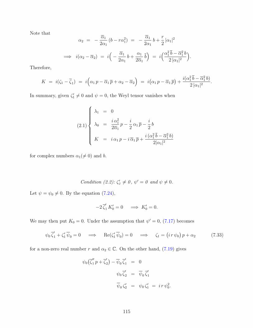
Note that
α2 = − α1
2α1
(b− rα21) = − α1
2α1
b+r
2|α1|2
=⇒ i(α2 − α2) = i(− α1
2α1
b+α1
2α1
b)
= i(α2
1 b− α21 b
2 |α1|2).
Therefore,
K = i(ζ1 − ζ1) = i(α1 p− α1 p+ α2 − α2
)= i
(α1 p− α1 p
)+i(α2
1 b− α21 b)
2 |α1|2.
In summary, given ζ ′1 6= 0 and ψ = 0, the Weyl tensor vanishes when
(2.1)
λ1 = 0
λ0 =i α2
1
2α1
p− i
2α1 p−
i
2b
K = i α1 p− i α1 p+i (α2
1 b− α21 b)
2|α1|2
for complex numbers α1(6= 0) and b.
Condition (2.2): ζ ′1 6= 0 , ψ′ = 0 and ψ 6= 0.
Let ψ = ψ0 6= 0. By the equation (7.24),
−2 ζ′1K
′0 = 0 =⇒ K ′0 = 0.
We may then put K0 = 0. Under the assumption that ψ′ = 0, (7.17) becomes
ψ0 ζ′1 + ζ ′1 ψ0 = 0 =⇒ Re(ζ ′1 ψ0) = 0 =⇒ ζ1 =
(i r ψ0
)p+ α2 (7.33)
for a non-zero real number r and α2 ∈ C. On the other hand, (7.19) gives
ψ0
(ζ′′1 p+ ζ
′2
)− ψ0 ζ
′1 = 0
ψ0 ζ′2 = ψ0 ζ
′1
ψ0 ζ′2 = ψ0 ζ
′1 = i r ψ2
0.
115

It implies that ζ ′2 =i r ψ2
0
ψ0
. Hence, ζ2 =(i r ψ2
0
ψ0
)p+ b for a complex constant b.
Since both ψ and K0 are constant functions, (7.18) becomes
− 2i ζ′1(ζ1 − ζ1) + i(ζ
′′1 p+ ζ
′2)(ζ ′1 p+ ζ2) + i ζ ′1(ζ
′1 p+ ζ2) = 0. (7.34)
By the formulas of ζ1 and ζ2, the left hand side of (7.34) becomes
−2i ζ′1(ζ1 − ζ1) + i(ζ
′′1 p+ ζ
′2)(ζ ′1 p+ ζ2) + i ζ ′1(ζ
′1 p+ ζ2)
= −2i(−i r ψ0)(i r ψ0 p+ α2 + i r ψ0 p− α2
)+ i(−i r ψ2
0
ψ0
)(i r ψ0 p+
i r ψ20
ψ0
p+ b)
+i(i r ψ0)[− i r ψ0 p+
(−i r ψ2
0
ψ0
)p+ b
]= −2 r ψ0
(i r ψ0 p+ i r ψ0 p+ α2 − α2
)+[i r2 ψ
2
0 p+ i r2 ψ0 ψ0 p+r ψ
2
0
ψ0
b]
−[− i r2 ψ0 ψ0 p− i r2 ψ
2
0 p+ r ψ0 b]
=(− 2i r2 |ψ0|2 + i r2 |ψ0|2 + i r2 |ψ0|2
)p+
(− 2i r2 ψ
2
0 + i r2 ψ2
0 + i r2 ψ2
0
)p
−2 r ψ0(α2 − α2) +r ψ
2
0
ψ0
b− r ψ0 b
=r
ψ0
(− 2 |ψ0|2(α2 − α2) + ψ
2
0 b− ψ20 b).
Therefore, (7.18) is satisfied when
− 2 |ψ0|2 (α2 − α2) + ψ2
0 b− ψ20 b = 0. (7.35)
When λ1 = ψ0, we have
λ0 = − x2
2ψ′(p)− i
2
(ζ ′1 p+ ζ2
)= − i
2
((i r ψ0
)p+
(i r ψ20
ψ0
)p+ b
).
Let α0 = i r ψ0. Noteψ0
ψ0
= −α0
α0
. The term λ0 becomes
λ0 = − i
2
(α0 p−
α20
α0
p)p− i
2b =
i α0
2α0
(α0 p− α0 p
)− i
2b. (7.36)
116
On the other hand, the function K is given by
K = i(ζ1 − ζ1) = i((i r ψ0
)p+ α2 −
(− i r ψ0
)p+ α2
)= i
(α0 p− α0 p
)+ i(α2 − α2).
(7.37)
Note that (7.35) is equivalent to
α2 − α2 =ψ
2
0 b− ψ20 b
2 |ψ0|2= − α0
2α0
b+α0
2α0
b =α2
0 b− α20 b
2|α0|2. (7.38)
Therefore, under the condition (2.2), the Weyl tensor vanishes when
(2.2)
λ1 =−i α0
r
λ0 =i α2
0
2α0
p− i
2α0 p−
i
2b
K = i α0 p− i α0 p+i (α2
0 b− α20 b)
2|α0|2
for complex numbers α0, b, and a real number r with α0 6= 0 and r 6= 0. Note that system
(2.1) is a special case to system (2.2) if we put r =∞ (λ1 = 0).
Condition (2.3): ζ ′1 6= 0 , ψ′′ = 0 and ψ′ 6= 0 .
Let ψ(p) = α1 p+ α2 with α1 6= 0. First of all, since K ′′0 = C = 0, (7.26) becomes
−2i ψ′K ′0 = −2i α1K
′0 = 0.
It implies that K ′0 = 0 and K0 is a constant function. Then, (7.24) gives
ψ′(ζ′′1 p+ ζ
′2
)− ζ ′1 ψ
′= 0 =⇒ α1
(ζ′′1 p+ ζ
′2
)= α1 ζ
′1. (7.39)
Differentiate (7.39) by p, and we have
α1 ζ′′1 = α1 ζ
′1 =⇒ Im(α1 ζ
′′1 ) = 0 =⇒ ζ ′′1 = r α1
for some r ∈ R. We may write ζ ′1(p) = r α1 p+ b for b ∈ C.
117

Back to (7.39),
α1
(r α1 p+ ζ
′2
)= α1
(r α1 p+ b
)=⇒ α1 ζ
′2 = α1 b =⇒ ζ ′2 =
α1 b
α1
Therefore, we may write ζ2(p) =(α1 b
α1
)p+ c for c ∈ C.
From our analysis on ψ, ζ1 and ζ2, (7.17) implies that
ψ ζ′1 + ζ ′1 ψ +
1
2ψ′(ζ′1 p+ ζ2
)+
1
2ψ′(ζ ′1 p+ ζ2
)= 0 (α1 p+ α2)(r α1 p+ b) + (r α1 p+ b)(α1 p+ α2)
+1
2α1
((r α1 p+ b) p+
α1 b
α1
p+ c)
+1
2α1
((r α1 p+ b) p+
α1 b
α1
p+ c) = 0.
(7.40)
The pp-terms of the left hand side of (7.40) gives
(r α1 α1
)p p+
(r α1 α1
)p p+
(1
2r α1 α1
)p+
(1
2r α1 α1
)p p = 3 |α1|2 r = 0.
Therefore, r = 0 and so ζ ′1 = b 6= 0. We put r = 0 to (7.40).
(α1 p+ α2) b+ (α1 p+ α2) b+1
2α1
(b p+
α1 b
α1
p+ c)
+1
2α1
(b p+
α1 b
α1
p+ c)
= 0
2α1 b p + 2α1 b p + α2 b + α2 b +1
2α1 c +
1
2α1c = 0.
So α1 b = 0. Under the condition (2.3), ψ′ = α1 6= 0, so we must have b = 0, which leads to
a contradiction. Hence, when ζ ′1 6= 0, ψ′′ = 0 and ψ 6= 0 occur, there is no solution set of λ1,
λ0 and K so that the Weyl tensor vanishes.
118
Theorem 7.3. Suppose in the local model (4.1) of D(w), the torsion function is defined by
w = λ0 + λ1 u+K u2 − λ1 u3 + λ0 u
4,
where λ0, λ1 and K satisfies the system (7.16). Then, the Weyl tensor W of D(w) vanishes
if and only if one of the following cases occurs.
Case(1.11) : λ1 ∈ C, λ0 = 0 and K = K(x2) for an arbitrary real-valued function.
Case(1.12) : λ1 ∈ C, λ0 ∈ C and K ∈ R for arbitrary constants.
Case(1.2) : λ1 = α1 p+ α2, λ0 = −α1
2(x2 − r) and K =
b
x2 − r
for arbitrary constants α1 (6= 0), α2 ∈ C and b, r ∈ R.
Case(2) : λ1 =i α
ror 0, λ0 =
i α2
2αp− i
2α p− i
2β
and K = i α p− i α p+i (α2 β − α2 β)
2|α|2
for arbitrary constants α (6= 0), β ∈ C and r ( 6= 0) ∈ R
As a remark to Theorem 7.3, if we express the solutions of λ1, λ0 and K above in terms of
(7.14), then we could obtain the respective φ functions, which are unique up to a R-linear
combination between |p|2 + x2, c1 p+ c1 p (c1 ∈ C), x2 and 1.
(1.11) : φ = x2
(λ1 p+ λ1 p
)− 2
∫ ∫K dx2 dx2
(1.12) : φ = x2
(λ1 p+ λ1 p
)− λ0 p
2 − λ0 p2 −K0 x
22
(1.2) : φ = x2
(α1
2p2 + α2 p+
α1
2p2 + α2 p
)− r α1
2p2 − r α1
2p2 − 2 b
∫ln(x2 − r) dx2
(2) : φ =i x2
r
(α p− α p
)+i
2|p|2(α p− α p
)− i
6|α|2(α3 p3 − α3 p3
)+i (α2 β − α2 β)
2|α|2|p|2 +
i
2
(β p2 − β p2
)
119

7.3 THE GENERAL SOLUTION
In addition to (7.13), the system (7.14) also gives a general form of λ0, λ1 and K solving
(7.1) in terms of an arbitrary real-valued function φ(p, p, x2):
λ1 = φpx2 , λ0 = −1
2φpp and K = φpp −
1
2φx2x2 .
We imposed an extra condition (7.15) to system (7.13) to solve for coefficients λ0, λ1 and
K so that W = 0. If we refer to the system (7.14), then the assumption on (7.15) is that
both φppy and φppp p0 are zero. If λ0, λ1 and K satisfies the format in (7.16),
λ1 = ψ, λ0 = −x2
2ψ′ − i
2
(ζ ′1 p+ ζ2
)and K = K0(x2) + i(ζ1 − ζ1),
then we have λ1,x2 = λ0,p p = 0. It implies that φppy = φppp p = 0.
On the other hand, if φppy = 0, then we get αppy = 0 by the definition of φ right before
(7.14). So there is a real-valued function σ of p and p such that α = x2(Ψ + Ψ) + σ. The
other condition φppp p = 0 is equivalent to σppp p = 0. It means that
σpp = γ(p) p+ γ1(p)
for two holomorphic functions γ and γ1. If Γ is a holomorphic antiderivative of γ, then we
get σpp = Γ + Γ up to a real constant. Therefore,
λ1 = ψ,
λ0 = −x2
2ψ′ − 1
2
(γ p+ γ1
)− i
2
(θ′′1 p+ θ′′2
)= − x2
2ψ′ − i
2
((θ′′1 − i γ)p+ (θ′′2 − i γ1)
),
K = (Γ + Γ) + i(θ′1 − θ1)− ρ(x2) = i(
(θ′1 − iΓ)− (θ′1 + iΓ)
)− ρ(x2).
We can now set ζ1 = θ′′1 − iΓ and ζ2 = θ′′2 − i γ1 to express λ0, λ1 and K in the format of
system (7.16).
120
Back to our main concern, we are going to extract a general condition on φ such that the
remaining terms in the Weyl tensor, W1212, W1215, W1515 and W1525 vanish.
Let F1, F2 and F3 be the following terns.
F1 =i
2
(φpp φpx2
)p− i
2
(φpx2 φpp
)p
+i
2
(φpp φpx2
)p− i
2
(φp p φpx2
)p
F2 = i(φ2px2
)p− i(φx2x2 φp p
)p
+ i(φ2pp
)p− i(|φpp|2
)p
F3 = i(φpp φpx2
)p− i(φpx2 φp p
)p
+i
2
(φ2px2
)x2− i
2
(φx2x2 φp p
)x2
(7.41)
Here,(φ2pp
)p
means((φpp)
2)p, and
(φ2px2
)p
means((φpx2)2
)p.
The termsW1212, W1215, W1515 andW1525 are polynomials of u and u with coefficients being
F1, F2, F3 or their complex conjugates.
Proposition 7.4.
W1212 = F1
(|u|8 − 2|u|6 − 6|u|4 − 2|u|2 + 1
)+F2
(u4 u3 + u3 u2 − u2 u− u
)+ F2
(u3 u4 + u2 u3 − uu2 − u
)+F3
(u4 u2 + 2u3 u+ u2
)+ F3
(u2 u4 + 2uu3 + u2
)W1215 =
3
2F1
(u2 u3 − u
)+
1
4F2
(3|u|4 + 2|u|2 − 1
)+
1
4F2
(3u2 + 2uu3 − u2 u4
)+
1
2F3
(u2 u+ u
)− 1
2F3
(uu4 + u3
)W1515 =
3
2F1 u
2 +1
2F2 u−
1
2F2 u
3 +1
4F3 +
1
4F3 u
4
W1525 =1
4F1
(|u|4 − 4|u|2 + 1
)+
1
4F2
(u2 u− u
)+
1
4F2
(uu2 − u
)+
1
4F3 u
2 +1
4F3 u
2
121

Therefore, these terms are zero when both of F1, F2 and F3 are zero. By Theorem 7.3, we
know that the system of (Fj = 0, j = 1, 2, 3) is consistent with non-trivial solution. The
formulas of Fj’s in (7.41) can be simplified using the Hessian of φ. We let
d2φ =
φpp φpp φpx2
φpp φp p φpx2
φpx2 φpx2 φx2x2
.
Let C be the cofactor matrix of d2φ. We have
C11 = φp p φx2x2 − φ2px2, C12 = |φpx2|2 − φpp φx2x2 , C22 = φpp φx2x2 − φ2
px2,
C13 = φpp φpx2 − φp p φpx2 , C23 = φpp φpx2 − φpp φpx2 , C33 = |φpp|2 − φ2pp.
Under this notation, we get to the following expression.F1 =
i
2
((C13
)p−(C23
)p
),
F2 = −i((
C11
)p
+(C33
)p
)F3 = i
(C13
)p− i
2
(C11
)x2
(7.42)
As an application of (7.41) and (7.42), we may consider an embedding of a 3-manifold to
a 4-manifold. The torsion function w is determined by the trace-free second fundamental
form. In particular, let M be R3 with coordinates (x1, x2, x3) and let f : R3 → R. We could
define an embedding from R3 to R4 by the graph of f :
F : R3 → R4, F (x1, x2, x3) =(x1, x2, x3, f(x1, x2, x3)
).
The fourth coordinate of R4 is labeled by t. For simplicity we assume that f depends on x1
only. An orthonormal frame for the image of F is given by e1, e2, e3 with
e1 =1√
1 + (f ′)2
( ∂
∂x1
+ f ′∂
∂t
), e2 =
∂
∂x2
and e3 =∂
∂x3
.
122
Moreover, let n be the unit normal to the image of F in the outward direction.
n =1√
1 + (f ′)2
( ∂∂t− f ′ ∂
∂x1
)The second fundamental form is given by
G0ij = II(ei, ej) = − gE
(∇ein, ej
),
where ∇ is the Riemannian connection of the Euclidean metric gE on R4. Explicitly, all G0ij’s
vanish except G011, where
G011 =
f ′′
(1 + (f ′)2)3/2.
Let q be the trace-free second fundamental form. We call the twistor CR structure of the
torsion tensor i q by Df . By (3.7) and (3.10), the torsion function w is obtained by
w = iuT ·C · q = − 1
2G0
11
(1− u2
)2.
We have already know that w is in the form of (4.12), where
λ1 = 0, λ0 = − f ′′
2(1 + (f ′)2)3/2and K =
f ′′
(1 + (f ′)2)3/2.
Moreover, λ0, λ1 and K solve the system (7.1) because we could find out a real-valued
function φ so that (7.14) is satisfied. Indeed, we can take
φ(x1) = 4
∫f ′√
1 + (f ′)2dx1.
It is then obvious that both F1, F2 and F3 are zero since φpp = φpp = (1/4)φ′′. There-
fore, the Weyl tensor of D(q) vanishes everywhere on the Fefferman bundle whenever f is
determined by x1 only.
In general, we have the following results when φ depends on a single variable only.
123

Theorem 7.5. Under the following choices of φ from (7.14), which defines the function
w = λ0 + λ1 u+K u2 − λ1 u3 + λ0 u
4,
the Weyl tensor of the respective CR structure D(w) on a flat space M vanishes.
(φ = φ(x1)) : λ1 = 0, λ0 = −1
8φx1x1 and K =
1
4φx1x1
(φ = φ(x2)) : λ1 = 0, λ0 = 0 and K = −1
2φx2x2
(φ = φ(x3)) : λ1 = 0, λ0 =1
8φx3x3 and K =
1
4φx3x3
As a remark, the case that φ = φ(x2) has been included in the case (1.11) of Theorem 7.3.
However, for φ = φ(x1) or φ = φ(x3), the conclusion in Theorem 7.5 is not covered since we
don’t necessarily have φppp p = 0 under the new hypothesis.
124
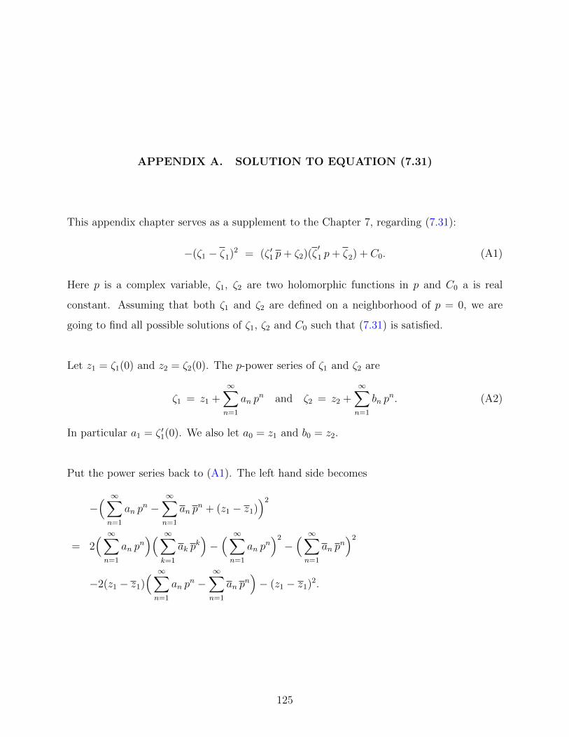
APPENDIX A. SOLUTION TO EQUATION (7.31)
This appendix chapter serves as a supplement to the Chapter 7, regarding (7.31):
−(ζ1 − ζ1)2 = (ζ ′1 p+ ζ2)(ζ′1 p+ ζ2) + C0. (A1)
Here p is a complex variable, ζ1, ζ2 are two holomorphic functions in p and C0 a is real
constant. Assuming that both ζ1 and ζ2 are defined on a neighborhood of p = 0, we are
going to find all possible solutions of ζ1, ζ2 and C0 such that (7.31) is satisfied.
Let z1 = ζ1(0) and z2 = ζ2(0). The p-power series of ζ1 and ζ2 are
ζ1 = z1 +∞∑n=1
an pn and ζ2 = z2 +
∞∑n=1
bn pn. (A2)
In particular a1 = ζ ′1(0). We also let a0 = z1 and b0 = z2.
Put the power series back to (A1). The left hand side becomes
−( ∞∑n=1
an pn −
∞∑n=1
an pn + (z1 − z1)
)2
= 2( ∞∑n=1
an pn)( ∞∑
k=1
ak pk)−( ∞∑n=1
an pn)2
−( ∞∑n=1
an pn)2
−2(z1 − z1)( ∞∑n=1
an pn −
∞∑n=1
an pn)− (z1 − z1)2.
125

And the right hand side becomes[( ∞∑n=1
n an pn−1)p+
∞∑n=1
bn pn + z2
] [( ∞∑n=1
n an pn−1)p+
∞∑n=1
bn pn + z2
]+ C1
= p p( ∞∑n=1
n an pn−1)( ∞∑
k=1
k ak pk−1)
+ p( ∞∑n=1
n an pn−1)( ∞∑
k=1
bk pk + z2
)+p( ∞∑n=1
n an pn−1)( ∞∑
k=1
bk pk + z2
)+( ∞∑k=1
bk pk + z2
)( ∞∑k=1
bk pk + z2
)+ C0
In genera, for k ≥ 1 and n ≥ 1, the pk pn-terms follow the formula:
2ak an = k ak · n an + (k + 1) ak+1 bn−1 + (n+ 1) an+1 bk−1 + bk bn. (A3)
Multiply both sides of (A3) by pn for n ≥ 1 and then take the sum over n from 1 to infinity.
2ak
∞∑n=1
an pn = k ak
( ∞∑n=1
n an pn)
+ (k + 1) ak+1
( ∞∑n=1
bn−1 pn)
+bk−1
( ∞∑n=1
(n+ 1) an+1 pn)
+ bk
( ∞∑n=1
bn pn)
2ak(ζ1 − z1) = k ak · p ζ′1 + (k + 1) ak+1 · p ζ2 + bk−1(ζ
′1 − a1) + bk(ζ2 − z2)
Take complex conjugate over the equation.
2(ζ1 − z1)ak = p ζ ′1 · k ak + p ζ2 · (k + 1) ak+1 + (ζ ′1 − a1)bk−1 + (ζ2 − z2)bk
Let q be another complex variable. For q ≥ 1, multiply qk and sum over k from 1 to infinity.
2(ζ1(p)− z1
)( ∞∑k=1
ak qk)
= p ζ ′1(p)( ∞∑k=1
k ak qk)
+ ζ ′1(p)( ∞∑k=1
bk−1 qk)
+p ζ2(p)( ∞∑k=1
(k + 1) ak+1 qk)
+ζ2(p)( ∞∑k=1
bk qk)− a1
( ∞∑k=1
bk−1 qk)− z2
( ∞∑k=1
bk qk)
2(ζ1(p)− z1
)(ζ1(q)− z1
)= p ζ ′1(p) · q ζ ′1(q) + ζ ′1(p) · q ζ2(q) + p ζ2(p)
(ζ′1(q)− a1
)+ ζ2(p)
(ζ2(q)− z2
)− a1 q ζ2(q)− z2
(ζ2(q)− z2
)
126
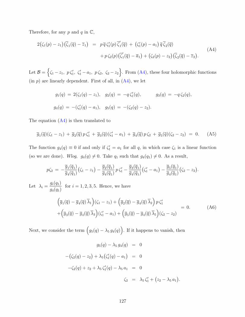
Therefore, for any p and q in C,
2(ζ1(p)− z1
)(ζ1(q)− z1
)= p q ζ ′1(p) ζ
′1(q) +
(ζ ′1(p)− a1
)q ζ2(q)
+ p ζ2(p)(ζ′1(q)− a1
)+(ζ2(p)− z2
)(ζ2(q)− z2
).
(A4)
Let B =ζ1− z1, p ζ
′1, ζ
′1−a1, p ζ2, ζ2− z2
. From (A4), these four holomorphic functions
(in p) are linearly dependent. First of all, in (A4), we let
g1(q) = 2(ζ1(q)− z1), g2(q) = −q ζ ′1(q), g3(q) = −q ζ2(q),
g4(q) = −(ζ ′1(q)− a1), g5(q) = −(ζ2(q)− z2).
The equation (A4) is then translated to
g1(q)(ζ1 − z1) + g2(q) p ζ ′1 + g3(q)(ζ ′1 − a1) + g4(q) p ζ2 + g5(q)(ζ2 − z2) = 0. (A5)
The function g4(q) ≡ 0 if and only if ζ ′1 = a1 for all q, in which case ζ1 is a linear function
(so we are done). Wlog, g4(q) 6= 0. Take q1 such that g4(q1) 6= 0. As a result,
pζ2 = −g1(q1)
g4(q1)
(ζ1 − z1
)− g2(q1)
g4(q1)p ζ ′1 −
g3(q1)
g4(q1)
(ζ ′1 − a1
)− g5(q1)
g4(q1)
(ζ2 − z2
).
Let λi =gi(q1)
g4(q1)for i = 1, 2, 3, 5. Hence, we have
(g1(q)− g4(q)λ1
)(ζ1 − z1) +
(g2(q)− g4(q)λ2
)p ζ ′1
+(g3(q)− g4(q)λ3
)(ζ ′1 − a1) +
(g5(q)− g4(q)λ5
)(ζ2 − z2)
= 0. (A6)
Next, we consider the term(g5(q)− λ5 g4(q)
). If it happens to vanish, then
g5(q)− λ5 g4(q) = 0
−(ζ2(q)− z2
)+ λ5
(ζ ′1(q)− a1
)= 0
−ζ2(q) + z2 + λ5 ζ′1(q)− λ5 a1 = 0
ζ2 = λ5 ζ′1 +
(z2 − λ5 a1
).
127
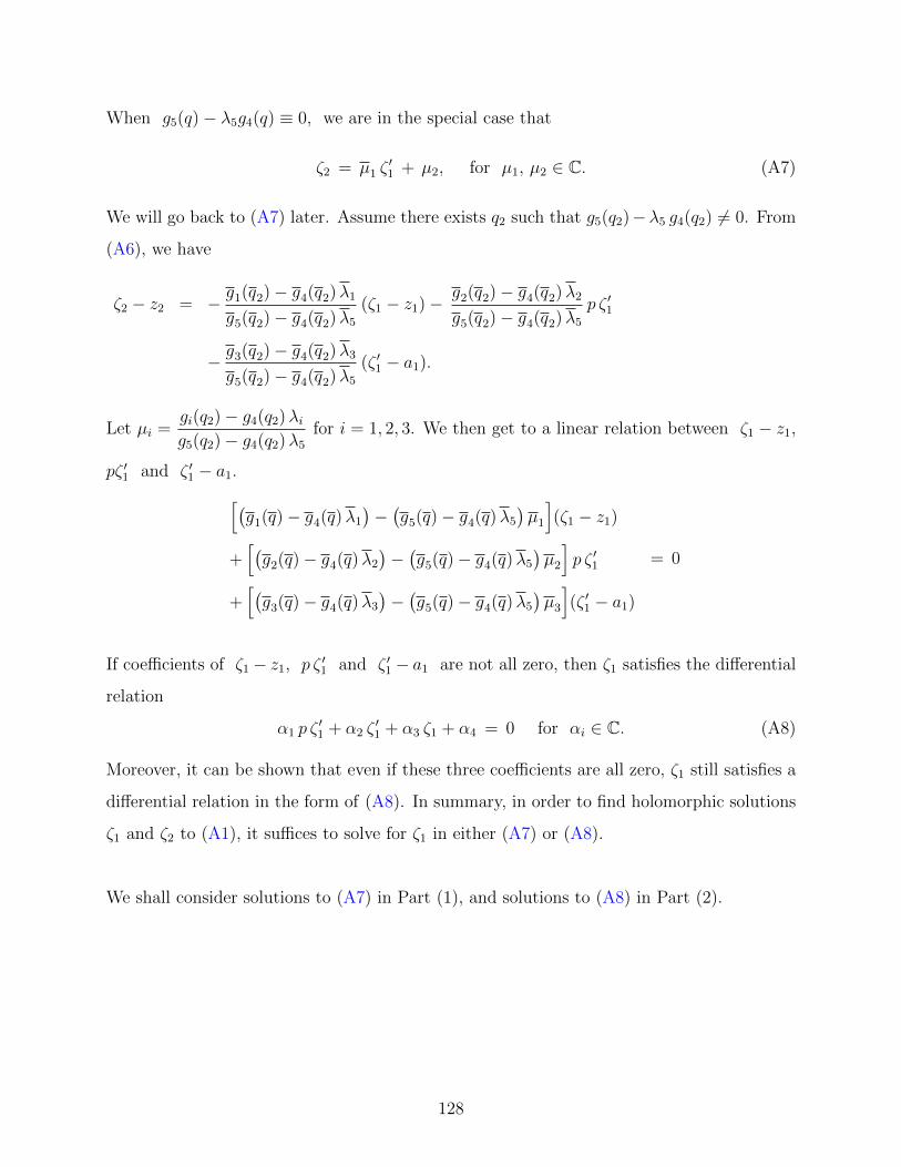
When g5(q)− λ5g4(q) ≡ 0, we are in the special case that
ζ2 = µ1 ζ′1 + µ2, for µ1, µ2 ∈ C. (A7)
We will go back to (A7) later. Assume there exists q2 such that g5(q2)−λ5 g4(q2) 6= 0. From
(A6), we have
ζ2 − z2 = − g1(q2)− g4(q2)λ1
g5(q2)− g4(q2)λ5
(ζ1 − z1)− g2(q2)− g4(q2)λ2
g5(q2)− g4(q2)λ5
p ζ ′1
− g3(q2)− g4(q2)λ3
g5(q2)− g4(q2)λ5
(ζ ′1 − a1).
Let µi =gi(q2)− g4(q2)λig5(q2)− g4(q2)λ5
for i = 1, 2, 3. We then get to a linear relation between ζ1 − z1,
pζ ′1 and ζ ′1 − a1.[(g1(q)− g4(q)λ1
)−(g5(q)− g4(q)λ5
)µ1
](ζ1 − z1)
+[(g2(q)− g4(q)λ2
)−(g5(q)− g4(q)λ5
)µ2
]p ζ ′1
+[(g3(q)− g4(q)λ3
)−(g5(q)− g4(q)λ5
)µ3
](ζ ′1 − a1)
= 0
If coefficients of ζ1 − z1, p ζ ′1 and ζ ′1 − a1 are not all zero, then ζ1 satisfies the differential
relation
α1 p ζ′1 + α2 ζ
′1 + α3 ζ1 + α4 = 0 for αi ∈ C. (A8)
Moreover, it can be shown that even if these three coefficients are all zero, ζ1 still satisfies a
differential relation in the form of (A8). In summary, in order to find holomorphic solutions
ζ1 and ζ2 to (A1), it suffices to solve for ζ1 in either (A7) or (A8).
We shall consider solutions to (A7) in Part (1), and solutions to (A8) in Part (2).
128
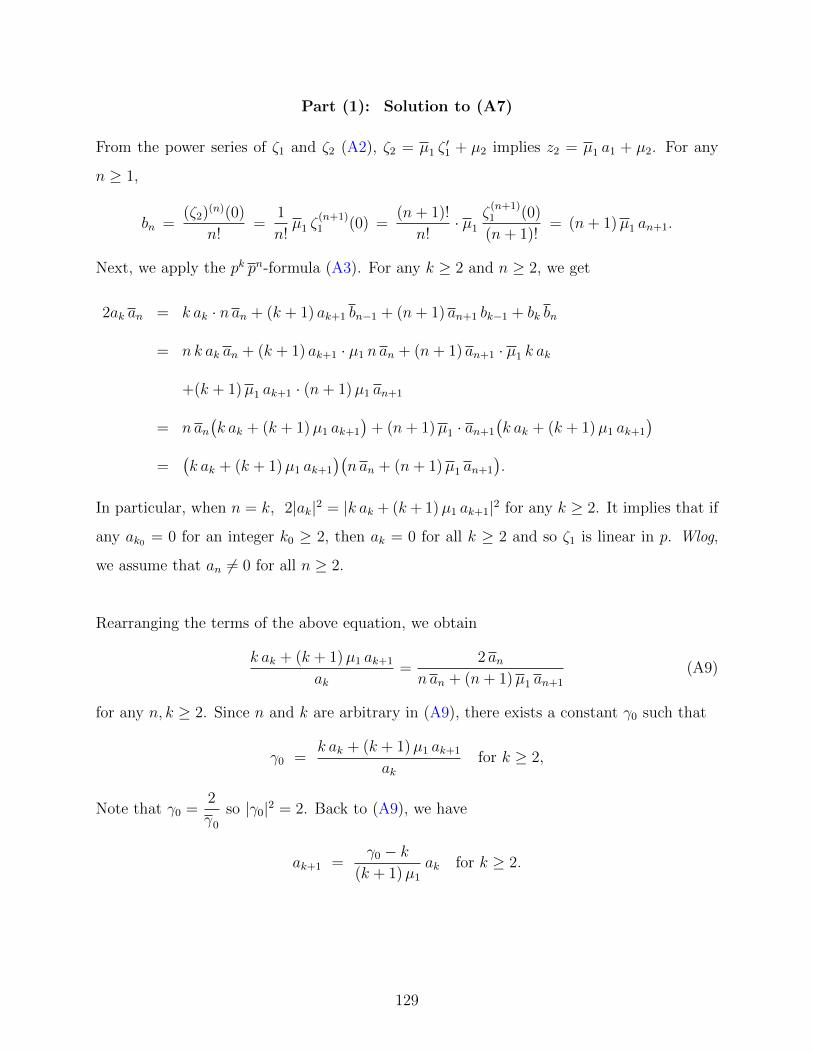
Part (1): Solution to (A7)
From the power series of ζ1 and ζ2 (A2), ζ2 = µ1 ζ′1 + µ2 implies z2 = µ1 a1 + µ2. For any
n ≥ 1,
bn =(ζ2)(n)(0)
n!=
1
n!µ1 ζ
(n+1)1 (0) =
(n+ 1)!
n!· µ1
ζ(n+1)1 (0)
(n+ 1)!= (n+ 1)µ1 an+1.
Next, we apply the pk pn-formula (A3). For any k ≥ 2 and n ≥ 2, we get
2ak an = k ak · n an + (k + 1) ak+1 bn−1 + (n+ 1) an+1 bk−1 + bk bn
= n k ak an + (k + 1) ak+1 · µ1 n an + (n+ 1) an+1 · µ1 k ak
+(k + 1)µ1 ak+1 · (n+ 1)µ1 an+1
= n an(k ak + (k + 1)µ1 ak+1
)+ (n+ 1)µ1 · an+1
(k ak + (k + 1)µ1 ak+1
)=
(k ak + (k + 1)µ1 ak+1
)(n an + (n+ 1)µ1 an+1
).
In particular, when n = k, 2|ak|2 = |k ak + (k+ 1)µ1 ak+1|2 for any k ≥ 2. It implies that if
any ak0 = 0 for an integer k0 ≥ 2, then ak = 0 for all k ≥ 2 and so ζ1 is linear in p. Wlog,
we assume that an 6= 0 for all n ≥ 2.
Rearranging the terms of the above equation, we obtain
k ak + (k + 1)µ1 ak+1
ak=
2 ann an + (n+ 1)µ1 an+1
(A9)
for any n, k ≥ 2. Since n and k are arbitrary in (A9), there exists a constant γ0 such that
γ0 =k ak + (k + 1)µ1 ak+1
akfor k ≥ 2,
Note that γ0 =2
γ0
so |γ0|2 = 2. Back to (A9), we have
ak+1 =γ0 − k
(k + 1)µ1
ak for k ≥ 2.
129

Recursively,
ak+1 =γ0 − k
(k + 1)µ1
ak =
(γ0 − k
)(γ0 − (k − 1)
)(k + 1) k µ2
1
ak−1
=(γ0 − k)(γ0 − k + 1) · · · (γ0 − 2)
(k + 1) k · · · 3µk−11
a2
=(γ0 − k)(γ0 − k + 1) · · · (γ0 − 2)(γ0 − 1)γ0
(k + 1)!µk+11
· 2 a2 µ21
γ0(γ0 − 1).
We are to find f(p) = c0 +∑∞
n=1 cn pn such that cn = an for all n ≥ 2. Indeed,
f(p) =2 a2 µ
21
γ0(γ0 − 1)
( pµ1
+ 1)γ0
implies that f (n)(0)/(n!) = an for all n ≥ 2. Therefore, for some d1, d2 ∈ C,
ζ1 =2a2µ
21
γ0(γ0 − 1)
( pµ1
+ 1)γ0
+ d1 p+ d2. (A10)
Differentiate (A10) by p to get
ζ ′1 =2 a2 µ1
γ0 − 1
( pµ1
+ 1)γ0−1
+ d1.
By the relation ζ2 = µ1 ζ′1 + µ2,
ζ2 =2a2 |µ1|2
γ0 − 1
( pµ1
+ 1)γ0−1
+ µ1 d1 + µ2. (A11)
For the moment, we go back to the main equation (A1). The holomorphic part of (A1) gives
2ζ1 ζ1 − ζ21 − ζ
2
1 = p p ζ ′1 ζ′1 + p ζ
′1 ζ2 + p ζ ′1 ζ2 + ζ2 ζ2 + C0
=⇒ 2ζ1 ζ1(0)− ζ21 − ζ
2
1(0) = p ζ′1(0) ζ2 + ζ2 ζ2(0) + C0
−(ζ1 − z1
)2=(a1 p+ z2
)ζ2 + C0.
Therefore,
ζ2 =−(ζ1 − z1)2 + (z1 − z1)2 + z2 z2
a1 p+ z2
. (A12)
130
We can equalize (A11) and (A12).
2a2 |µ1|2
γ0 − 1
( pµ1
+ 1)γ0−1
+ µ1 d1 + µ2 =−(
2a2 µ21
γ0(γ0−1)
(pµ1
+ 1)γ0 + d1 p+ d2 − z1
)2
− C0
a1 p+ z2
(a1 p+z2
)[2a2 |µ1|2
γ0 − 1
( pµ1
+1)γ0−1
+µ1 d1+µ2
]= −
( 2a2 µ21
γ0(γ0 − 1)
( pµ1
+1)γ0+d1 p+d2−z1
)2
−C0.
Let y =p
µ1
+ 1. The above equation becomes
(a1µ1(y−1)+z2
)[2a2|µ1|2
γ0 − 1yγ0−1+µ1d1+µ2
]= −
( 2a2µ21
γ0(γ0 − 1)yγ0 +d1µ1(y−1)+d2−z1
)2
−C0.
On left hand side, powers of y are: yγ0 , yγ0−1, y, 1.
On right hand side, powers of y are: y2γ0 , yγ0+1, yγ0 , y2, y, 1.
The coefficient of y2γ0 on the right hand side is −(
2a2µ21
γ0(γ0−1)
)2
6= 0. So we may have
2γ0 = γ0, 2γ0 = γ0 − 1, 2γ0 = 1, or 2γ0 = 0.
Hence, γ0 = 0, − 1 or 1/2. None of them gives |γ0|2 = 2. We arrive at a contradiction to
such a constant γ0 exists. The only possible case in (A7) is that an = 0 for all n ≥ 2. So ζ1
is linear in p.
131

Part (2): Solution to (A8)
The equation (A8): α1 p ζ′1 + α2 ζ
′1 + α3 ζ1 + α4 = 0 for αi ∈ C, is an ordinary differential
equation which could be solved to different solutions.
(I) Both α1 6= 0 and α3 6= 0 : ζ1(p) = c1
(p+ α
)γ+ c2 for c1, c2, α, γ ∈ C.
(II) α1 = 0 and α3 6= 0 (α2 6= 0) : ζ1(p) = c1 eγp + c2 for c1, c2, γ ∈ C.
(III) α3 = 0 and α1 6= 0 (α4 6= 0) : ζ1(p) = c1 log(α1 p+ α2
)+ c2 for cj, αj ∈ C
(IV) Both α1 = 0 and α3 = 0 : ζ1 is a linear function in p.
We would work on the case (I) while a similar method is applied to show that there is no
solution from case (II) or case (III) satisfying (A1).
Let ζ1(p) = c1(p+ α)γ + c2. We have
ζ ′1 = c1 γ(p+ α)γ−1, z1 = ζ1(0) = c1 αγ + c2, and a1 = ζ ′1(0) = c1 γ α
γ−1. (A13)
Denote y = p+ α. The LHS of (A1) becomes
−(ζ1 − ζ1)2 = −(c1(p+ α)γ − c1(p+ α)γ + c2 − c2
)2
= −(c1(p+ α)γ − c1(p+ α)γ
)2
−2(c2 − c2)(c1(p+ α)γ − c1(p+ α)γ
)− (c2 − c2)2
= −c21 (p+ α)2γ − c2
1 (p+ α)2γ + 2|c1|2 (p+ α)γ(p+ α)γ
−2c1(c2 − c2)(p+ α)γ + 2c1(c2 − c2)(p+ α)γ − (c2 − c2)2
−(ζ1 − ζ1)2 = −c21 y
2γ − c21 y
2γ + 2|c1|2 yγ yγ − 2c1(c2 − c2) yγ
+2c1(c2 − c2) yγ − (c2 − c2)2.
Moreover, we have
C0 = −(z1 − z1)2 − |z2|2 = −(c1 α
γ − c1 αγ + c2 − c2
)2 − |z2|2
= 2|c1|2 αγ αγ − c21 α
2γ − c21 α
2γ − (c2 − c2)2 − 2c1(c2 − c2)αγ + 2c1(c2 − c2)αγ − |z2|2.
132

From the formula in (A12),
ζ2 =−(ζ1(p)− z1)2 − C0
w1p+ z2
=−(c1(p+ α)γ + c2 − c2 − c1α
γ)2 − C0
a1p+ z2
=
−c21 (p+ α)2γ − 2c1
(c2 − c2 − c1α
γ)(p+ α)γ + c2
1 α2γ
+2c1αγ(c2 − c2 − c1α
γ) + |z2|2
a1p+ z2
.
Note that
a1p+ z2 = a1(p+ α) + (z2 − a1α) = a1y + (z2 − a1α),
a1p+ z2 = a1(p+ α) + (z2 − a1α) = a1y + (z2 − a1α).
As a result,
ζ2 =
(− c2
1 y2γ − 2c1(c2 − c2 − c1α
γ)yγ + c21 α
2γ + 2c1αγ(c2 − c2 − c1α
γ) + |z2|2)
a1y + (z2 − a1α).
We then rewrite (A1) in the form of
−|a1p+z2|2(ζ1− ζ1)2 =(
(a1p+z2)(ζ ′1p+ ζ2))(
(a1p+z2)(ζ′1p+ ζ2)
)+C0|a1p+z2|2. (A14)
On the left of (A14), we get
−|a1p+ z2|2(ζ1 − ζ1
)2=
(|a1|2yy + (z2 − a1α)a1y + (z2 − a1α)a1y + |z2 − a1α|2
)·
−c21y
2γ − c21y
2γ + 2|c1|2yγyγ
−2c1(c2 − c2)yγ + 2c1(c2 − c2)yγ − (c2 − c2)2
.
Regarding the right hand side of (A14), we first find out
ζ ′1p+ ζ2 = ζ ′1(p+ α)− αζ ′1 + ζ2 = c1γ(p+ α)γ−1(p+ α)− αc1γ(p+ α)γ−1
+1
w1p+ z2
−c21(p+ α)2γ − 2c1(c2 − c2 − c1α
γ)(p+ α)γ
+c21α
2γ + 2c1αγ(c2 − c2 − c1α
γ) + |z2|2
.
133
It leads to the expression of (a1p+ z2)(ζ ′1p+ ζ2).
(a1p+ z2)(ζ ′1p+ ζ2)
=(a1(p+ α) + (z2 − a1α)
)·(c1γ(p+ α)γ−1(p+ α)− αc1γ(p+ α)γ−1
)+(− c2
1(p+ α)2γ − 2c1(c2 − c2 − c1αγ)(p+ α)γ + c2
1α2γ
+ 2c1αγ(c2 − c2 − c1α
γ) + |z2|2)
= a1c1γ(p+ α)γ(p+ α) + (z2 − a1α)c1γ(p+ α)γ−1(p+ α) − a1αc1γ(p+ α)γ
− (z2 − a1α)αc1γ(p+ α)γ−1 − c21(p+ α)2γ − 2c1(c2 − c2 − c1α
γ)(p+ α)γ
+ c21α
2γ + 2c1αγ(c2 − c2 − c1α
γ) + |z2|2
= a1c1γyγy + (z2 − a1α)c1γy
γ−1y − a1αc1γyγ − (z2 − a1α)αc1γy
γ−1 − c21y
2γ
− 2c1(c2 − c2 − c1αγ)yγ + c2
1α2γ + 2c1α
γ(c2 − c2 − c1αγ) + |z2|2
Overall, the right hand side of (A14) is as follows.((a1p+ z2)(ζ ′1p+ ζ2)
)((a1p+ z2)(ζ
′1p+ ζ2)
)+ C0|a1p+ z2|2
=
a1c1γyγy + (z2 − a1α)c1γy
γ−1y − a1αc1γyγ − (z2 − a1α)αc1γy
γ−1 − c21y
2γ
− 2c1(c2 − c2 − c1αγ)yγ + c2
1α2γ + 2c1α
γ(c2 − c2 − c1αγ) + |z2|2
·
a1c1γyyγ + (z2 − a1α)c1γyy
γ−1 − a1αc1γyγ − (z2 − a1α)αc1γy
γ−1 − c21y
2γ
− 2c1(c2 − c2 − c1αγ)yγ + c2
1α2γ + 2c1α
γ(c2 − c2 − c1αγ) + |z2|2
−(
(c1αγ − c1α
γ + c2 − c2)2 + |z2|2)
·(|a1|2|y|2 + (z2 − a1α)a1y + (z2 − a1α)a1y + |z2 − a1α|2
)We are ready to compare the exponents of y and y on two sides of (A14). On the left, there
are 24 different exponents of y or y:
y2γ+1y, yy2γ+1, y2γ+1, y2γ+1, y2γy, yy2γ, y2γ, y2γ,
yγ+1yγ+1, yγ+1yγ, yγyγ+1, yγ+1y, yyγ+1, yγ+1, yγ+1,
yγyγ, yγy, yyγ, yγ, yγ, yy, y, y, 1.
134

On the right hand side of (A14), there 32 different kind of exponents of y or y:
y2γ+1yγ, yγy2γ+1, y2γ+1yγ−1, yγ−1y2γ+1,
y2γy2γ, y2γyγ, yγy2γ, y2γyγ−1, yγ−1y2γ, y2γ, y2γ,
yγ+1yγ+1, yγ+1yγ, yγyγ+1, yγ+1yγ−1, yγ−1yγ+1,
yγyγ, yγyγ−1, yγ−1yγ, yγy, yyγ, yγ, yγ,
yγ−1yγ−1, yγ−1y, yyγ−1, yγ−1, yγ−1, yy, y, y, 1.
From the right of (A14), the coefficient of y2γ y2γ is |c1|4 6= 0. This term must belong to an
exponent of y and y on the left hand side. If it is represented by a real monomial yδ yδ on
the left, then we have
2γ = γ + 1, 2γ = γ, 2γ = 1 or 2γ = 0.
So γ = 0, 1/2 or 1 in this situation.
On the other hand, it may happen that y2γ y2γ is represented by a complex monomial yδ1 yδ2
on the left, which happens to be real-valued with a particular γ. We may have
2γ = 2γ + 1 = 1, 2γ = 2γ + 1 = 0, 2γ = 2γ = 1, 2γ = 2γ = 0,
2γ = 2γ + 1 = γ, 2γ = γ + 1 = 1, 2γ = γ + 1 = 0, 2γ = γ = 1
2γ = γ = 0, 2γ = 1 = 0, or 2γ = 0.
From any one of the above equalities, we must have γ = 0 or 1/2. When γ = 1/2, note that
the coefficient of y2γ+1 yγ on the right is −|c1|2c1a1γ with
a1 = c1 γ αγ−1 =
c1
2α−1/2 6= 0.
So y2γ+1 yγ is a non-zero term when γ = 1/2. On the left, we have exponents of y or y from:
y2y, yy2, y2, y2, yy, yy, y, y, y3/2y3/2, y3/2y1/2, y1/2y3/2, y3/2y,
yy3/2, y3/2, y3/2, y1/2y1/2, y1/2y, yy1/2, y1/2, y1/2, yy, y, y, 1.
135
There is no y2 y1/2 term on the left hand side, so we arrive at a contradiction. γ 6= 1/2. It
means that γ = 0 or 1. γ = 0 is a trivial case, and when γ = 1, ζ1 is linear in p. We have
shown that the possible solutions of ζ1 to (A8), is either a constant or a linear function in p.
At the end of our analysis, we explore what happens when ζ1 is exactly a linear function in
p. Let ζ1(p) = a0 + a1 p with a1 6= 0. Consider (A3) with n = 1 and k ≥ 1, we get
2 a1 ak = k a1 ak + (k + 1) ak+1 b0 + 2 a2 bk−1 + b1 bk = k a1 ak + b1 bk.
It means (2−k) a1 ak = b1 bk for any k ≥ 1. Put k = 1, we have |a1|2 = |b1|2 6= 0. So, b1 6= 0.
Whenever k ≥ 2, the left hand side is zero, so bk = 0 for all k ≥ 2. In other words, we may
let ζ2 = b0 + b1 p with b0, b1 ∈ C.
Here we may apply the formula for ζ2 in (A12). We have
ζ2 =−(ζ1 − a0)2 + (a0 − a0)2 + |b0|2
a1 p+ b0
=−a2
1 p2 − 2a1(a0 − a0) p+ |b0|2
a1 p+ b0
.
It implies that (a1 p+ b0)(b1 p+ b0) = −a21 p
2− 2a1(a0− a0) p+ |b0|2. By comparison, we get
a1 b1 = −a21 and b0 b1 + a1 b0 = −2a1(a0 − a0).
On solving, the first equation gives b1 = −a21
a1
. The second equation is equivalent to
i(a2
1 b0 − a21 b0
)= − 2i |a1|2
(a0 − a0
).
A general solution to the above equation is
b0 = − 2 a1 a0
a1
+ k a21 for any k ∈ R.
Therefore, ζ2 = − a21
a1
p− 2 a1 a0
a1
+ k a21 for any real number k.
136
APPENDIX B. PROOF OF THEOREM 6.2
This appendix is to justify Theorem 6.2 in order to complete our logical argument. We will
mainly follow the notations from J. M. Lee’s paper [11] on Fefferman metric (but with the
Levi form multiplied by a factor of 2) and also refer to [4]. Moreover, since we are proving a
general result in CR geometry, notations and variables defined in the following will be used
exclusively to the current chapter.
The statement of Theorem 6.2 is as follows. The definition of the Chern tensor follows from
(1.5), and that of the Weyl tensor from (1.15) and (1.16).
Theorem. Let N be a CR manifold of hypersurface type on which the CR structure L is
non-degenerate. Let ν be the CR dimension of L. Associated with the contact form θ, let C
be the Chern curvature tensor and F be the Fefferman metric on C(N). Suppose W is the
Weyl tensor of F . Then,
(1) : Cmnkl = W(Tm, Tn, Tk, Tl) for every m, n, k, l.
(2) : W(Tm, Tn, Z1, Z2) = 0 for any m,n. Z1, Z2 are tangent vectors on C(N).
To begin with, let B =T1, T2, · · · , Tν
be the basis for the holomorphic bundle T 1,0N and
T1, T2, · · · , Tν
be the basis for the antiholomorphic bundle T 0,1N . With respect to the
contact form θ, let Lθ be the Levi form and T0 (= T ) be the Reeb vector field.
137

The derivative of θ is
dθ = 2i hαβ θα ∧ θβ for hαβ = Lθ(Tα, Tβ). (B1)
Define g to be the Webster metric associated with θ. ∇ is the Tanaka-Webster connection
on N such that its Christoffel symbols are given by
∇TαTβ = Γγαβ Tγ, ∇TαTβ = Γγαβ Tγ and ∇T0Tβ = Γγ0β Tγ. (B2)
Letθ1, θ2, · · · , θν
be the dual coframe of B and so θα = θα is the dual 1-form of Tα. The
connection forms of ∇ are then defined by
ωγβ = Γγαβ θα + Γγαβ θ
α + Γγ0β θ. (B3)
Here we write Γγαβ
= (Γγαβ), Γγαβ
= (Γγαβ) and Γγ0β
= (Γγ0β). Also, we have
dhαβ = hαγ ωγ
β+ hγβ ω
αγ , (B4)
with ωγβ
= ωγβ . Similar to the Cartan first structural equation, we have
dθα = θβ ∧ ωαβ + θ ∧ τα and dθα = θβ ∧ ωαβ + θ ∧ τ α. (B5)
In this way, the Lie brackets between Tα, Tβ and T0 are found by[Tα, Tβ] = −2i hαβ T0 − Γγ
βαTγ + Γγ
αβTγ
[Tα, Tβ] =(Γγαβ − Γγβα
)Tγ
[Tα, T0] = −Γγ0α Tγ + Aγα Tγ
(B6)
The τ -operator in (B5) is defined by: for any X on TN ,
τ(X) = tor(T0, X) = ∇T0X − [T0, X].
It allows us to write
τ = τα ⊗ Tα + τ α ⊗ Tα with τα = Aαβ θβ and τ α = Aαβ θ
β. (B7)
138

The coefficients Aβα’s appear both in (B6) and (B7). We can find them by the formula
Aβα = −hβγ g([T0, Tα], Tγ
).
The lower-index of Aβα by g is defined by Aαγ = Aβα hγβ. Taking the complex conjugation,
Aβα = (Aβα) and Aαγ = (Aαγ).
Correspondingly, the lower-index of the (1,1)-tensor τ is denoted by A, which is a (0,2)-tensor
given by A(u, v) = g(τ(u), v
)for any u, v on TN . Note that τ is self-adjoint with respect
to g, so Aαγ = Aγα. It implies that
Aγα = hγβ Aδβ hαδ and Aγα = hβγ Aδβ hδα. (B8)
We would also compute for the covariant derivative of A by ∇. Let
∇σAαλ =(∇TσA
)(Tα, Tλ
)= Tσ(Aαλ)− Aδλ Γδσα − Aαδ Γδσλ
Let V βαλ = hσβ∇σAαλ and V β
αµ = hσβ∇αAµσ. We also have
Vλ∆=
ν∑α=1
V ααλ =
ν∑α=1
V ααλ. (B9)
Following by τ , we look into the Ricci tensor of ∇. Let R be the Riemann tensor.
R(u, v)Tα = 2(dωβα − ωγα ∧ ωβγ
)(u, v)⊗ Tα (B10)
The curvature form on the RHS of (B10) is found by
dωβα − ωγα ∧ ωβγ = Rαβλµ θ
λ ∧ θµ + V βαλ θ
λ ∧ θ − V β
αλθλ ∧ θ
+2i hαγ θγ ∧ τβ + 2i hαγ θ
β ∧ τ γ
= Rαβλµ θ
λ ∧ θµ + V βαλ θ
λ ∧ θ − V β
αλθλ ∧ θ
+2i Aδα θβ ∧ θδ + 2i hαγA
β
δθγ ∧ θδ.
(B11)
139
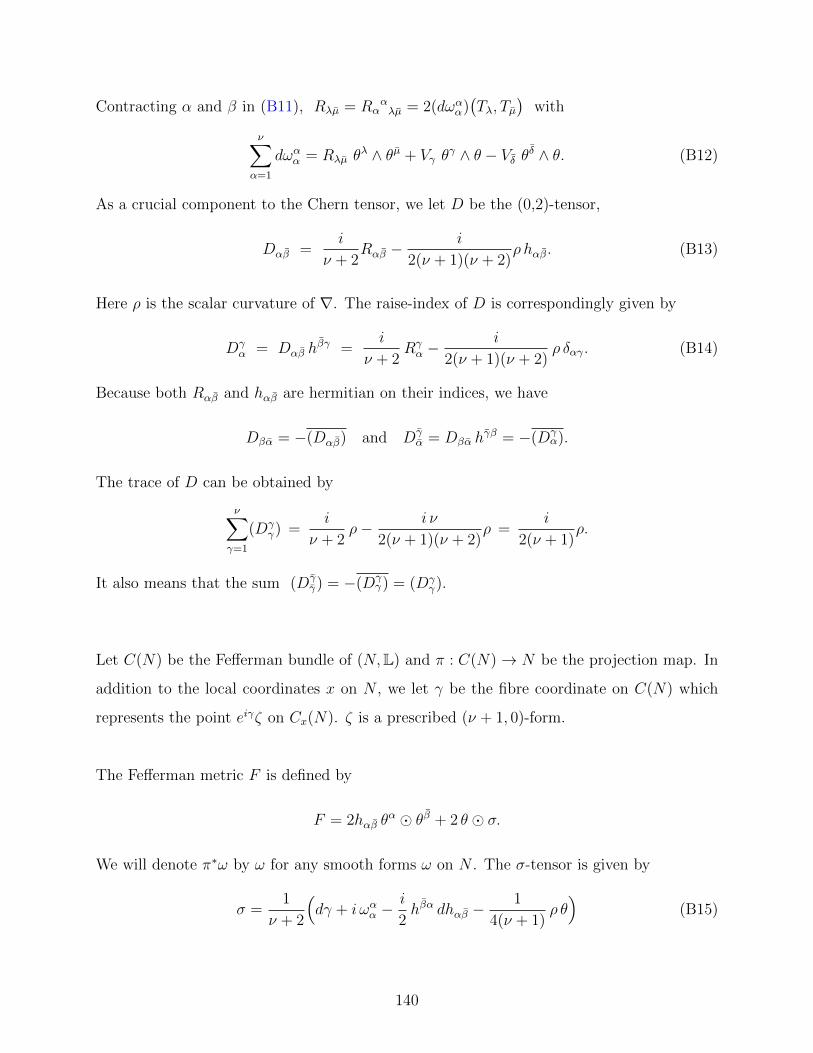
Contracting α and β in (B11), Rλµ = Rααλµ = 2(dωαα)
(Tλ, Tµ
)with
ν∑α=1
dωαα = Rλµ θλ ∧ θµ + Vγ θ
γ ∧ θ − Vδ θδ ∧ θ. (B12)
As a crucial component to the Chern tensor, we let D be the (0,2)-tensor,
Dαβ =i
ν + 2Rαβ −
i
2(ν + 1)(ν + 2)ρ hαβ. (B13)
Here ρ is the scalar curvature of ∇. The raise-index of D is correspondingly given by
Dγα = Dαβ h
βγ =i
ν + 2Rγα −
i
2(ν + 1)(ν + 2)ρ δαγ. (B14)
Because both Rαβ and hαβ are hermitian on their indices, we have
Dβα = −(Dαβ) and Dγα = Dβα h
γβ = −(Dγα).
The trace of D can be obtained by
ν∑γ=1
(Dγγ) =
i
ν + 2ρ− i ν
2(ν + 1)(ν + 2)ρ =
i
2(ν + 1)ρ.
It also means that the sum (Dγγ) = −(Dγ
γ) = (Dγγ).
Let C(N) be the Fefferman bundle of (N,L) and π : C(N)→ N be the projection map. In
addition to the local coordinates x on N , we let γ be the fibre coordinate on C(N) which
represents the point eiγζ on Cx(N). ζ is a prescribed (ν + 1, 0)-form.
The Fefferman metric F is defined by
F = 2hαβ θα θβ + 2 θ σ.
We will denote π∗ω by ω for any smooth forms ω on N . The σ-tensor is given by
σ =1
ν + 2
(dγ + i ωαα −
i
2hβα dhαβ −
1
4(ν + 1)ρ θ)
(B15)
140

Let Z be a moving frame on C(N) which consists of vectors Zα, Zα, Z0 and Zc. (1 ≤ α ≤ ν).
Zα = Tα −i
2
(Γγαγ − Γγαγ
) ∂∂γ
Zα = Tα −i
2
(Γγαγ − Γγαγ
) ∂∂γ
Z0 = T0 −( i
2
(Γα0α − Γα0α
)− ρ
4(ν + 1)
) ∂∂γ
Zc = (ν + 2)∂
∂γ
The matrix representation of F corresponding to Z =Z0, Z1, · · · , Zν , Z1, · · ·Zν , Zc
, is
[F ] =
0 0 0 1
0 0ν[hαβ]
0
0[hβα]
0ν 0
1 0 0 0
and [F−1] =
0 0 0 1
0 0ν[hβα]
0
0[hαβ]
0ν 0
1 0 0 0
.
Here α and β are the respective row and column indices.
The Lie brackets between vectors in Z are described by
[Zα, Zβ] =(Γγαβ − Γγβα
)Zγ,
[Zα, Zβ] = −2i hαβ Z0 − ΓγβαZγ + Γγ
αβZγ −Dαβ Zc,
[Zα, Z0] = −Γγ0α Zγ + Aγα Zγ +( 1
4(ν + 1)(ν + 2)Tα(ρ)− i
(ν + 2)Vα
)Zc.
(B16)
In the following context, an index of capital letters runs within the set
0, 1, · · · , ν, 1, · · · ν, c
.
For example, if X = ξP ZP is a vector field on C(N). then it means
X = ξ0 Z0 + ξ1 Z1 + · · ·+ ξν Zν + ξ1 Z1 + · · ·+ ξν Zν + ξc Zc.
Meanwhile, an index of Greek or small letters runs from 1 to ν only, or from 1 to ν.
141
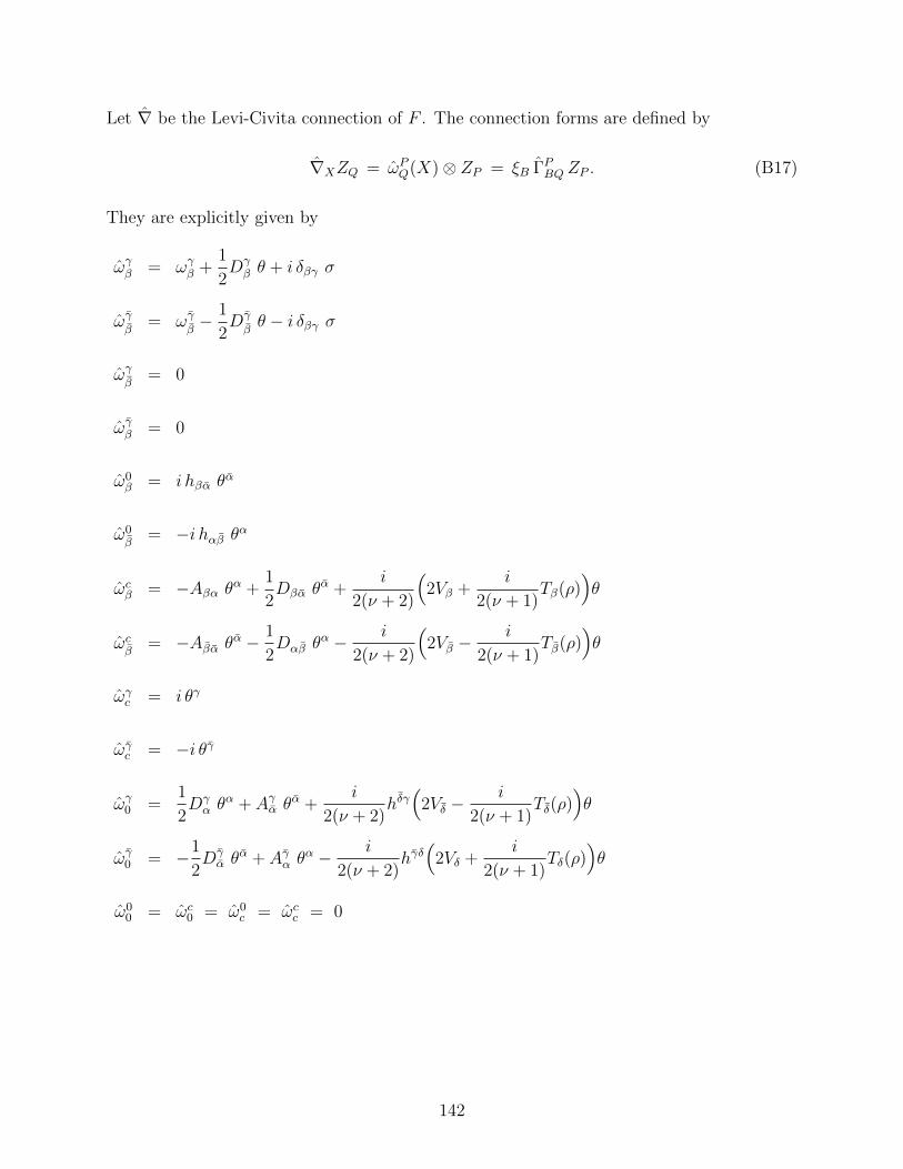
Let ∇ be the Levi-Civita connection of F . The connection forms are defined by
∇XZQ = ωPQ(X)⊗ ZP = ξB ΓPBQ ZP . (B17)
They are explicitly given by
ωγβ = ωγβ +1
2Dγβ θ + i δβγ σ
ωγβ
= ωγβ− 1
2Dγ
βθ − i δβγ σ
ωγβ
= 0
ωγβ = 0
ω0β = i hβα θ
α
ω0β
= −i hαβ θα
ωcβ = −Aβα θα +1
2Dβα θ
α +i
2(ν + 2)
(2Vβ +
i
2(ν + 1)Tβ(ρ)
)θ
ωcβ
= −Aβα θα −1
2Dαβ θ
α − i
2(ν + 2)
(2Vβ −
i
2(ν + 1)Tβ(ρ)
)θ
ωγc = i θγ
ωγc = −i θγ
ωγ0 =1
2Dγα θ
α + Aγα θα +
i
2(ν + 2)hδγ(
2Vδ −i
2(ν + 1)Tδ(ρ)
)θ
ωγ0 = −1
2Dγα θ
α + Aγα θα − i
2(ν + 2)hγδ(
2Vδ +i
2(ν + 1)Tδ(ρ)
)θ
ω00 = ωc0 = ω0
c = ωcc = 0
142

Part (1): Proof of Wmnkl = Cmnkl
We assume R to be the Riemann tensor and Ric to be the Ricci tensor of ∇. We set up the
notation that
R(ZP , ZQ)ZJ = RKPQJ ZK = 2 ΩK
J (ZP , ZQ)⊗ ZK ,
RPQJK = RAPQJ fAK and RPQ = Ric(ZP , ZQ).
(B18)
The symbol fAK means the metric coefficient F (ZA, ZK). Let S be the scalar curvature.
The Weyl tensor (1.15) of ∇, restricted to T 1,0N ⊕ T 0,1N , is represented by
Wmnkl = W(Zm, Zn, Zk, Zl)
= Rmnkl −1
2ν
(Rml fkn + Rkn fml − Rmk fnl − Rnl fmk
)+
S
(2ν)(2ν + 1)
(fml fkn − fmk fnl
)= Rmnkl −
1
2ν
(Rml fkn + Rkn fml
)+
S
(2ν)(2ν + 1)fml fkn
(B19)
and so on. Note that ι ∂∂γW = 0. So
Wmnkl = W(Zm, Zn, Zk, Zl) = W(Tm, Tn, Tk, Tl).
Together with the symmetry that Wmnkl =Wklmn, we are going to show that
Wmnkl = Cklmn
for any m, n, k and l. To begin with, we find out Rmnkl by
Rpmnk = 2 Ωp
k(Zm, Zn) = 2(dωpk − ω
Qk ∧ ω
pQ
)(Zm, Zn) (B20)
143
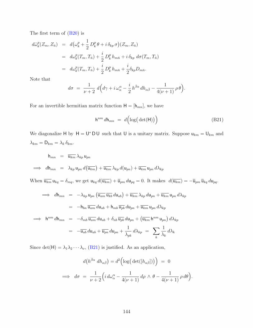
The first term of (B20) is
dωpk(Zm, Zn) = d(ωpk +
1
2Dpk θ + i δkp σ
)(Zm, Zn)
= dωpk(Tm, Tn) +i
2Dpk hmn + i δkp dσ(Tm, Tn)
= dωpk(Tm, Tn) +i
2Dpk hmn +
i
2δkpDmn.
Note that
dσ =1
ν + 2d(dγ + i ωαα −
i
2hβα dhαβ −
1
4(ν + 1)ρ θ).
For an invertible hermitian matrix function H = [hmn], we have
hnm dhmn = d(
log(
det(H)))
(B21)
We diagonalize H by H = U∗DU such that U is a unitary matrix. Suppose ukm = Ukm and
λkm = Dkm = λk δkm.
hmn = ukm λkp upn
=⇒ dhmn = λkp upn d(ukm)
+ ukm λkp d(upn) + ukm upn dλkp
When ukm ukq = δmq, we get ukq d(ukm) + upm dupq = 0. It makes d(ukm) = −upm ukq dupq.
=⇒ dhmn = −λkp upn(uam ukb duab
)+ ukm λkp dupn + ukm upn dλkp
= −hbn uam duab + hmb upb dupn + ukm upn dλkp
=⇒ hnm dhmn = −δmb uam duab + δnb upb dupn +(ukm hnm upn
)dλkp
= −uab duab + upn dupn +1
λpkdλkp =
∑k
1
λkdλk
Since det(H) = λ1λ2 · · ·λν , (B21) is justified. As an application,
d(hβα dhαβ
)= d2
(log(
det([hαβ])))
= 0
=⇒ dσ =1
ν + 2
(i dωαα −
1
4(ν + 1)dρ ∧ θ − 1
4(ν + 1)ρ dθ
).
144
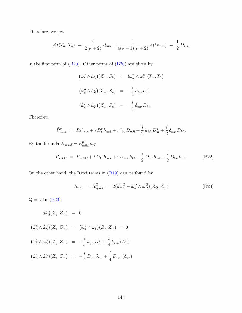
Therefore, we get
dσ(Tm, Tn) =i
2(ν + 2)Rmn −
1
4(ν + 1)(ν + 2)ρ (i hmn) =
1
2Dmn
in the first term of (B20). Other terms of (B20) are given by(ωγk ∧ ωpγ
)(Zm, Zn) =
(ωγk ∧ ω
pγ
)(Tm, Tn)
(ω0k ∧ ω
p0
)(Zm, Zn) = − i
4hknD
pm
(ωck ∧ ωpc
)(Zm, Zn) = − i
4δmpDkn
Therefore,
Rpmnk = Rk
pmn + iDp
k hmn + i δkpDmn +i
2hknD
pm +
i
2δmpDkn.
By the formula Rmnkl = Rpmnk hpl,
Rmnkl = Rmnkl + iDkl hmn + iDmn hkl +i
2Dml hkn +
i
2Dkn hml. (B22)
On the other hand, the Ricci terms in (B19) can be found by
Rmn = RQQmn = 2
(dωQn − ωPn ∧ ω
QP
)(ZQ, Zm) (B23)
Q = γ in (B23):
dωγn(Zγ, Zm) = 0
(ωkn ∧ ω
γk
)(Zγ, Zm) =
(ωkn ∧ ω
γ
k
)(Zγ, Zm) = 0
(ω0n ∧ ω
γ0
)(Zγ, Zm) = − i
4hγnD
γm +
i
4hmn (Dγ
γ)
(ωcn ∧ ωγc
)(Zγ, Zm) = − i
4Dγn δmγ +
i
4Dmn (δγγ)
145

Therefore,(dωγn − ωPn ∧ ω
γP
)(Zγ, Zm) =
i
4hγnD
γm −
i
4hmn (Dγ
γ) +i
4Dmn −
i
4ν Dmn.
Q = γ in (B23):
dωγn(Zγ, Zm) = dωγn(Tγ, Tm) +i
2hmγD
γn + iδnγ ·
1
(ν + 2)
( i2Rmγ −
i
4(ν + 1)ρhmγ
)= dωγn(Tγ, Tm) +
i
2hmγ D
γn +
i
2Dmn
(ωkn ∧ ω
γ
k
)(Zγ, Zm) =
(ωkn ∧ ω
γ
k
)(Tγ, Tm)(
ω0n ∧ ω
γ0
)(Zγ, Zm) = − i
4hmn (Dγ
γ)(ωcn ∧ ωγc
)(Zγ, Zm) = − i
4Dmn (δγγ)
Therefore,(dωγn − ωPn ∧ ω
γP
)(Zγ, Zm) =
1
2Rmn +
i
2hmγ D
γn +
i
2Dmn +
i
4hmn (Dγ
γ) +i
4ν Dmn.
Q = 0 in (B23):
dω0β = d
(i hβα θ
α)
= i hβγ ωγα ∧ θα + i hγα ω
γβ ∧ θ
α + i hβα θγ ∧ ωαγ + i hβα θ ∧ τ α
dω0β
= d(− i hαβ θα
)= − i hγβ ωγα ∧ θα − i hαγ ω
γ
β∧ θα − i hαβ θγ ∧ ωαγ − i hαβ θ ∧ τα
It implies that
dω0n(Z0, Zm) = − i
2Γγ0m hγn −
i
2Γγ0n hmγ +
i
2Γα0m hαn = − i
2Γγ0n hmγ.
Moreover, we have(ωPn ∧ ω0
P
)(Z0, Zm) =
(ωγn ∧ ω0
γ
)(Z0, Zm) = − i
2Γγ0n hmγ +
i
4Dγn hmγ.
Therefore,(dω0
β − ωPn ∧ ω0P
)(Z0, Zm) = − i
4Dγn hmγ.
146

Q = c in (B23):
dωcn(Zc, Zm) = 0(ωPn ∧ ωcP
)(Zc, Zm) =
(ωγn ∧ ωcγ
)(Zc, Zm) =
i
4Dmn
Therefore,(dωcβ − ωPn ∧ ωcP
)(Zc, Zm) = − i
4Dmn.
Combining everything, we get
Rmn = 2( i
4Dmn −
i
4hmn (Dγ
γ) +i
4Dmn −
i
4ν Dmn
)+2(1
2Rmn +
i
2Dmn +
i
2Dmn +
i
4hmn (Dγ
γ) +i
4ν Dmn
)− i
2Dmn −
i
2Dmn
= Rmn + 2iDmn.
As a result,
Rmn = Rmn + 2iDmn = Rmn + 2i( i
ν + 2Rmn −
i
2(ν + 1)(ν + 2)ρ hmn
)=⇒ Rmn =
ν
ν + 2Rmn +
1
(ν + 1)(ν + 2)ρ hmn
(B24)
The Chern tensor (assoicated with θ on N) is defined by C(Tm, Tn)Tk = Ckpmn Tp, where
Ckpmn = Rk
pmn −
1
ν + 2
(Rpk hmn +Rp
m hkn + δkp Rmn + δmp Rkn
)+
ρ
(ν + 1)(ν + 2)
(δkp hmn + δmp hkn
)=⇒ Cklmn = Rklmn −
1
ν + 2
(Rkl hmn +Rml hkn +Rmn hkl +Rkn hml
)+
ρ
(ν + 1)(ν + 2)
(hkl hmn + hml hkn
).
The D-tensor defined above plays a similar role to the Schouten tensor in Riemannian
geometry. We can express Cklmn in terms of the coefficients of the D-tensor.
147

Cklmn = Rklmn + i( i
ν + 2Rkl −
i
2(ν + 1)(ν + 2)ρ hkl
)hmn
+ i( i
ν + 2Rml −
i
2(ν + 1)(ν + 2)ρ hml
)hkn
+ i( i
ν + 2Rmn −
i
2(ν + 1)(ν + 2)ρ hmn
)hkl
+ i( i
ν + 2Rkn −
i
2(ν + 1)(ν + 2)ρ hkn
)hml
=⇒ Cklmn = Rklmn + i(Dkl hmn +Dml hkn +Dmn hkl +Dkn hml
)Show that Wmnkl = Cklmn
We will apply the statement of Theorem 1.4, S =2ν + 1
ν + 1ρ, in the work-out.
Wmnkl = Rklmn + iDkl hmn + iDmn hkl +i
2Dml hkn +
i
2Dkn hml (Rmnkl)
− hkn2ν
( ν
ν + 2Rml +
1
(ν + 1)(ν + 2)ρ hml
)(Rml)
− hml2ν
( ν
ν + 2Rkn +
1
(ν + 1)(ν + 2)ρ hkn
)(Rkn)
+1
(2ν)(2ν + 1)
(2ν + 1
ν + 1
)ρ hml hkn (S)
= Rklmn + iDkl hmn + iDmn hkl +i
2Dml hkn +
i
2Dkn hml
+i hkn
2
( i
ν + 2Rml −
i
2(ν + 1)(ν + 2)ρ hml
)+i hml
2
( i
ν + 2Rkn −
i
2(ν + 1)(ν + 2)ρ hkn
)− hkn hml
2ν(ν + 1)(ν + 2)ρ− hkn hml
2ν(ν + 1)(ν + 2)ρ
− hkn hml4(ν + 1)(ν + 2)
ρ− hkn hml4(ν + 1)(ν + 2)
ρ+1
2ν(ν + 1)ρ hml hkn
= Rklmn + iDkl hmn + iDmn hkl +i
2Dml hkn +
i
2Dkn hml
+i
2hknDml +
i
2hmlDkn
= Rklmn + iDkl hmn + iDmn hkl + iDml hkn + iDkn hml
= Cklmn
148

Therefore, we justify that Wklmn =Wmnkl = Cmnkl for every m, n, k, l.
Part (2): W(Tm, Tn, u1, u2
)= 0 when u1, u2 are on T 1,0N ⊕ T 0,1N
(2.1) Show Wmnkl = 0. Note that Wmnkl = Rmnkl = Rpmnk hlp and
Rpmnk = 2
(dωpk − ω
Qk ∧ ω
pQ
)(Zm, Zn).
The first term dωpk = 0 and
(ωQk ∧ ω
pQ
)(Zm, Zn) =
(ω0k ∧ ω
p0 + ωck ∧ ωpc
)(Zm, Zn) = 0.
Therefore, Wmnkl = Rmnkl = 0.
(2.2) Show Wmnkl = 0. By definition,
Wmnkl = Rmnkl −1
2νRnk hml +
1
2νRmk hnl. (B25)
The first term of (B25) is Rmnkl = Rpmnk hpl with Rp
mnk = 2(dωpk − ω
Qk ∧ ω
pQ
)(Zm, Zn).
dωpk(Zm, Zn) = dωpk(Tm, Tn) + iδkp dσ(Zm, Zn) = dωpk(Tm, Tn)
(ωQk ∧ ω
pQ
)(Zm, Zn) = (ωγk ∧ ωpγ)(Zm, Zn) + (ωck ∧ ωpc )(Zm, Zn)
= (ωγk ∧ ωpγ)(Tm, Tn) +
i
2
(Akn δmp − Akm δnp
)Therefore,
Rpmnk = 2
(dωpk − ω
γk ∧ ω
pγ
)(Tm, Tn)− i
(Akn δmp − Akm δnp
)= Rk
pmn − i
(Akn δmp − Akm δnp
)= 2i
(Ank δmp − Amk δnp
)− i(Akn δmp − Akm , δnp
)= i
(Ank δmp − Amk δnp
).
149

In the third step above, we apply the formula regarding Rkpmn:
Rkpmn = 2
(dωpk − ω
γk ∧ ω
pγ
)(Tm, Tn) =
(2i δmpAkn − 2i δnpAkm
). (B26)
(B26) will be justify later in Part (3).
On the other hand, Rmk = 2∑P,Q
(dωQk − ω
Pk ∧ ω
QP
)(ZQ, Zm).
(Q = γ)(dωγk − ωPk ∧ ω
γP
)(Zγ, Zm) =
1
2Rγγmk
=1
2
ν∑γ=1
(i Amk δγγ − i Aγk δmγ
)=
i ν
2Amk −
i
2Amk
(Q = γ)(dωγk − ωPk ∧ ω
γP
)(Zγ, Zm) = −
(ω0k ∧ ω
γ0
)(Zγ, Zm)−
(ωck ∧ ωγc
)(Zγ, Zm)
= −1
2(i hkl)(A
γm) +
1
2(−Akm)(−i δγγ)
= − i2Akm +
i ν
2Akm
(Q = 0)(dω0
k − ωPk ∧ ω0P
)(Z0, Zm) = i hkα dθ
α(T0, Tm)− (ωγk ∧ ω0γ)(Z0, Zm)
= i hkα
(1
2Aαm
)=
i
2Akm
(Q = c)(dωck − ωPk ∧ ωcP
)(Zc, Zm) = −(ωγk ∧ ω
cγ)(Zc, Zm)
= −1
2(i δkγ)(−Aγm) =
i
2Akm
As a result, Rmk = 2i (ν − 1)Amk + 2i Amk = 2i ν Amk. Hence,
Wmnkl = i(Ank δmp − Amk δnp
)hpl −
1
2νhml(2i ν Ank
)+
1
2νhnl(2i νAmk
)= i Ank hml − i Amk hnl − i Ank hml + i Amk hnl
= 0.
150

(2.3) Show Wmnk l = 0. We would need the formula :
Wmnkl = Rmnkl −1
2ν
(Rml hnk + Rnk hml − Rmk hnl − Rnl hmk
)+
S
(2ν)(2ν + 1)
(hml hnk − hmk hnl
)Note that Rmnkl = Rp
mnkhpl.
Rp
mnk= 2
(dωp
k− ωPk ∧ ω
pP
)(Zm, Zn) = − 2
(ω0k ∧ ω
p0
)(Zm, Zn)− 2
(ωck ∧ ω
pc
)(Zm, Zn)
= −2(− i
4hmkD
pn +
i
4hnkD
pm
)− 2(− i
4Dmk δnp +
i
4Dnk δmp
)=
i
2
(hmkD
pn − hnkDp
m +Dmk δnp −Dnk δmp
)Therefore, Rmnkl =
i
2
(hmkDnl − hnkDml +Dmk hnl −Dnk hml
).
Wmnkl
=i
2
(hmkDnl − hnkDml +Dmk hnl −Dnk hml
)− 1
2ν
(hnk(Rml + 2iDml) + hml(Rnk + 2iDnk)− hnl(Rmk + 2iDmk)− hmk(Rnl + 2iDnl)
)+
S
(2ν)(2ν + 1)
(hml hnk − hmk hnl
)=
i
2·( i
ν + 2
)(hmk Rnl − hnk Rml + hnlRmk − hmlRnk
)[first line]
+ρ
4(ν + 1)(ν + 2)
(hmk hnl − hnk hml + hmk hnl − hnk hml
)[first line]
− 1
2ν·(
1− 2
ν + 2
)(hnk Rml + hmlRnk − hnlRmk − hmk Rnl
)[2nd line]
− 1
2ν·( ρ
(ν + 1)(ν + 2)
)(2hnk hml − 2hnl hmk
)[2nd line]
+ρ
(2ν)(ν + 1)
(hml hnk − hmk hnl
)[3rd line]
= hmk Rnl
(− 1
2(ν + 2)+
1
2ν
( ν
ν + 2
))+ hnk Rml
(1
2(ν + 2)− 1
2ν
( ν
ν + 2
))+hnlRmk
(− 1
2(ν + 2)+
1
2ν
( ν
ν + 2
))+ hmlRnk
(1
2(ν + 2)− 1
2ν
( ν
ν + 2
))+hmk hnl ρ
( 2
4(ν + 1)(ν + 2)+
2
2ν(ν + 1)(ν + 2)− 1
2ν(ν + 1)
)+hnk hml ρ
(− 2
4(ν + 1)(ν + 2)− 2
2ν(ν + 1)(ν + 2)+
1
2ν(ν + 1)
)= 0
151

Part (3): W(Tm, Tn, u1, u2
)= 0 for any u1, u2 on C(N)
Recall that g is the Webster metric associated with θ. Let ∇ be the Levi-Civita connection
of g. Define Let ∇ be the Levi-Civita connection of g. Define (T = T0)∇TαTβ = Γγαβ Tγ + Γγαβ Tγ + Γ0
αβ T,
∇TαTβ = Γγαβ Tγ + Γγαβ Tγ + Γ0αβ T,
∇TTβ = Γγ0β Tγ + Γγ0β Tγ + Γ00β T
(B27)
We could obtain the Christoffel symbols in (B27) from the identities below.
∇TmTn = ∇TmTn − Amn T ∇TmTn = ∇TmTn − Amn T
∇TmTn = ∇TmTn + i hnm T ∇TmTn = ∇TmTn − i hmn T
∇TTm = ∇TTm + i Tm ∇TTm = ∇TTm − i Tm
∇TmT = i Tm + Akm Tk ∇TmT = −i Tm + Akm Tk ∇TT = 0
Let R be the Riemann tensor of ∇. We will find R(Tm, Tn)Tk.
R(Tm, Tn)Tk = ∇Tm∇TnTk − ∇Tn∇TmTk − ∇[Tm,Tn]Tk
∇Tm∇TnTk = ∇Tm
(∇TnTk − Akn T
)= Tm(Γγnk) + Γγnk ∇TmTγ − Tm(Akn)T − Akn ∇TmT
= Tm(Γγnk) + Γγnk∇TmTγ − Γγnk Amγ T − Tm(Akn)T − Akn(i Tm + Aγm Tγ
)= ∇Tm∇TnTk − i Akn Tm − AknAγm Tγ −
(Tm(Akn) + Γγnk Amγ
)T
∇Tn∇TmTk = ∇Tn∇TmTk − i Akm Tn − AkmAγn Tγ −(Tn(Akm) + Γγmk Anγ
)T
∇[Tm,Tn]Tk = (Γγmn − Γγnm)(∇TγTk − Aγk T
)= ∇[Tm,Tn]Tk − Aγk
(Γγmn − Γγnm
)T
152

Therefore,
R(Tm, Tn)Tk = R(Tm, Tn)Tk + i Akm Tn − i Akn Tm +(AkmA
γn − AknAγm
)Tγ
+(Tn(Akm)− Tm(Akn) + Γγmk Anγ − Γγnk Amγ + Aγk
(Γγmn − Γγnm
))T.
(B28)
Next we find R(Tk, T )Tm.
R(Tk, T )Tm = ∇Tk∇TTm − ∇T ∇TkTm − ∇[Tk,T ]Tm
∇Tk∇TTm = ∇Tk
(∇TTm + i Tm
)= Tk(Γ
γ0m)Tγ + Γγ0m
(∇TkTγ − Akγ T
)+ iΓγkm Tγ − i Amk T
= ∇Tk∇TTm + iΓγkm Tγ −(i Amk + Akγ Γγ0m
)T
∇T ∇TkTm = ∇T
(∇TkTm − Amk T
)= T (Γγkm)Tγ + Γγkm
(∇TTγ + i Tγ
)− T (Amk)T
= ∇T∇TkTm + iΓγkm Tγ − T (Amk)T
∇[Tk,T ]Tm = −Γγ0k ∇TγTm + Aγk ∇TγTm
= −Γγ0k(∇TγTm − Amγ T
)+ Aγk
(∇TγTm + i hmγ T
)= ∇[Tk,T ]Tm +
(Γγ0k Amγ + i Amk
)T
Therefore,
R(Tk, T )Tm = R(Tk, T )Tm +(T (Amk)− Akγ Γγ0m − Amγ Γγ0k − 2i Amk
)T. (B29)
153

(B28), (B29): Show that Wmnk0 = 0.
Wmnk0 = Rmnk0 = Rcmnk = 2
(dωck − ωPk ∧ ωcP
)(Zm, Zn)
dωck(Zm, Zn) = −(dAkα ∧ θα + Akα dθ
α)(Zm, Zn)
= −(dAkα ∧ θα + Akα θ
β ∧ ωαβ)(Zm, Zn)
= −1
2
(Tm(Akn)− Tn(Akm)
)− 1
2Akα
(Γαnm − Γαmn
)=
1
2
(Tn(Akm)− Tm(Akn) + Akα Γαmn − Akα Γαnm
)(ωPk ∧ ωcP )(Zm, Zn) = (ωγk ∧ ω
cγ)(Zm, Zn)
=1
2
((Γγmk)(−Aγn)− (Γγnk)(−Aγm)
)=
1
2
(Aγm Γγnk − Aγn Γγmk
)Therefore,
Rcmnk =
1
2
(Tn(Akm)− Tm(Akn) + Akα Γαmn − Akα Γαnm + Aγn Γγmk − Aγm Γγnk
).
We know that Rk0mn = g(R(Tm, Tn)Tk, T
)= 0. From (B28),
Rcmnk = 0 ⇐⇒ R(Tm, Tn, Tk, T ) = g
(R(Tm, Tn)Tk, T
)= 0.
From (B29), we have R(Tm, Tn, Tk, T ) = R(Tk, T, Tm, Tn) = 0. It justifies that Wmnk0 = 0.
As another application of the Levi-Civita connection of g, we compute for R(Tk, Tl)Tm.
R(Tk, Tl)Tm = ∇Tk∇TlTm − ∇Tl
∇TkTm − ∇[Tk,Tl]Tm
∇Tk∇TlTm = ∇Tk
(∇Tl
Tm + i hml T)
= Tk(Γγ
lm)Tγ + Γγ
lm
(∇TkTγ − Akγ T
)+ i Tk(hml)T + i hml
(i Tk + Aγk Tγ
)= ∇Tk∇Tl
Tm − hml Tk + i hmlAγk Tγ +
(i hmδ Γδ
kl+ i hδl Γ
δkm − Γγ
lmAkγ)T
154

∇Tl∇TkTm = ∇Tl
(∇TkTm − Akm T
)= Tl(Γ
γkm)Tγ + Γγkm
(∇Tl
Tγ + i hγl T)− Tl(Akm)T − Akm
(− i Tl + Aγ
lTγ)
= ∇Tl∇TkTm − AkmA
γ
lTγ + i Akm Tl +
(− Tl(Akm) + i hγl Γ
γkm
)T
∇[Tk,Tl]Tm = −2i hkl
(∇TTm + i Tm
)− Γγ
lk
(∇TγTm − Amγ T
)+ Γγ
kl
(∇TγTm + i hmγ T
)= ∇[Tk,Tl]
Tm + 2hkl Tm +(i hmγ Γγ
kl+ Γγ
lkAmγ
)T
Therefore,
R(Tk, Tl)Tm = R(Tk, Tl)Tm − hml Tk + i hmlAγk Tγ
+(i hmδ Γδkl + i hδl Γ
δkm − Γγ
lmAkγ)T
+AkmAγ
lTγ − i Akm Tl +
(Tl(Akm)− i hγl Γ
γkm
)T
−2hkl Tm −(i hmγ Γγ
kl+ Γγ
lkAmγ
)T
= R(Tk, Tl)Tm + AkmAγ
lTγ − hml Tk − 2hkl Tm
+i hmlAγk Tγ − i Akm Tl +
(Tl(Akm)− Γγ
lmAkγ − Γγ
lkAmγ
)T
(B30)
(B28), (B30): Find Rkp
mn in (B26).
Rklmn = g(R(Tm, Tn)Tk, Tl
)= g
(R(Tm, Tn)Tk − i Akm Tn + i Akn Tm , Tl
)(B28)
= Rmnkl − i Akm hnl + i Akn hml
= Rklmn − i Akm hnl + i Akn hml
=(i hmlA
γk hnγ − i Akm hnl
)− i Akm hnl + i Akn hml (B30)
= 2i hmlAkn − 2i Akm hnl
Therefore, Rkpmn = Rklmn h
lp = 2i δmpAkn − 2i δnpAkm.
155
Show that Wmnk0 = 0.
It is the final part to prove Theorem 6.2. We first recall the equation (B12):
ν∑m=1
dωmm = Rλµ θλ ∧ θµ + Vλ θ
λ ∧ θ − Vµ θµ ∧ θ.
Differentiate both sides of (B12).
0 = d2ωmm = dRλµ ∧ θλ ∧ θµ +Rλµ
(dθλ ∧ θµ − θλ ∧ dθµ
)+d(Vλ) ∧ θλ ∧ θ + Vλ
(dθλ ∧ θ − θλ ∧ dθ
)−d(Vµ) ∧ θµ ∧ θ − Vµ
(dθµ ∧ θ − θµ ∧ dθ
)Acting on (Tm, Tn, Tk), we have
(dRλµ ∧ θλ ∧ θµ
)(Tm, Tn, Tk) =
1
6
(Tm(Rnk)− Tn(Rmk)
)(Rλµ dθ
λ ∧ θµ)(Tm, Tn, Tk) =
1
6Rλk
(Γλnm − Γλmn
)(Rλµ θ
λ ∧ dθµ)(Tm, Tn, Tk) =
1
6
(−Rmµ Γµ
nk+Rnµ Γµ
mk
)(Vλ θ
λ ∧ dθ)
=1
3
(Vm · ihnk − Vn · ihmk
).
Putting all together, for fixed m, n and k,
Tm(Rnk)− Tn(Rmk) +Rλk(Γλnm − Γλmn) +RmµΓµ
nk−RnµΓµ
mk+ 2iVn hmk − 2iVm hnk = 0.
Note that
Tm(Rnk) = Tm(Rpn hpk) = Tm(Rp
n)hpk +Rpn Tm(hpk)
=⇒ Tm(Rpn)hpk = Tm(Rnk)−Rq
n Tm(hqk).
As a result,
Tm(Rpn) = Tm(Rnk)h
kp −Rqn Γδmk hqδ h
kp −Rqn Γpmq for fixed m, n, p. (B31)
(1) Set p = m in (B31):
Tm(Rmn ) = Tm(Rnk)h
km −Rnδ Γδmk hkm −Rq
n Γmmq.
156

(2) Set p = m and switch n and m in (B31):
Tn(Rmm) = Tn(Rmk)h
km −Rmδ Γδnk hkm −Rq
m Γmnq
Therefore, for particular m and n,
Tm(Rmn )− Tn(Rm
m)
= hkm(Tm(Rnk)− Tn(Rmk)
)+Rmγ Γγ
nkhkm −Rnγ Γγ
mkhkm +Rq
m Γmnq −Rqn (Γmmq)
= hkm[Rλk(Γ
λmn − Γλnm) +Rnµ Γµ
mk−Rmµ Γµ
nk+ 2i Vm hnk − 2i Vn hmk
]+Rmγ Γγ
nkhkm −Rnγ Γγ
mkhkm +Rq
m Γmnq −Rqn (Γmmq).
Summing on m, we get to( ν∑m=1
Tm(Rmn ))− Tn(ρ) = − 2i (ν − 1)Vn +Rm
λ Γλmn −Rqn (Γmmq).
We could now obtain the divergence formula of the D-tensor.
Tγ(Dγm)−Dγ
α Γαγm +Dpm (Γγγp)
=i
ν + 2Tγ(R
γm)− i
2(ν + 1)(ν + 2)
(Tγ(ρ) δγm
)−( i
ν + 2Rγα −
i
2(ν + 1)(ν + 2)ρ δαγ
)Γαγm +
( i
ν + 2Rpm −
i
2(ν + 1)(ν + 2)ρ δpm
)Γγγp
=i
ν + 2
[Tm(ρ)− 2i(ν − 1)Vm +Rp
λ Γλpm −Rqm (Γppq)
]− i
2(ν + 1)(ν + 2)Tm(ρ)− i
ν + 2Rγα Γαγm +
i
ν + 2Rpm (Γγγp)
=i (2ν + 1)
2(ν + 1)(ν + 2)Tm(ρ) +
2(ν − 1)
(ν + 2)Vm
We conclude that
Tγ(Dγm)−Dγ
α Γαγm +Dpm (Γγγp) =
i (2ν + 1)
2(ν + 1)(ν + 2)Tm(ρ) +
2(ν − 1)
(ν + 2)Vm (B32)
157

As an important step, we have to find out Rm0.
Rm0 = 2(dωQ0 − ωP0 ∧ ω
QP
)(ZQ, Zm)
(1) (Q = γ)
dωγ0 (Zγ, Zm) =(1
2d(Dγ
α) ∧ θα +1
2Dγα dθ
α)
(Zγ, Zm)
=1
4
(Tγ(D
γm)− Tm(Dγ
γ))
+1
4Dγα
(Γαmγ − Γαγm
)(ωP0 ∧ ω
γP )(Zγ, Zm) = (ωp0 ∧ ωγp )(Zγ, Zm) =
1
4Dpγ Γγmp −
1
4Dpm (Γγγp)
Therefore,(dωγ0 − ωP0 ∧ ω
γP
)(Zγ, Zm) =
1
4
(Tγ(D
γm)− Tm(Dγ
γ) +Dγα(Γαmγ − Γαγm)−Dp
γ Γγmp +Dpm(Γγγp)
).
(2) (Q = γ)
dωγ0 (Zγ, Zm)
=(− 1
2d(Dγ
α) ∧ θα − 1
2Dγα dθ
α + dAγα ∧ θα + Aγα dθα)
(Zγ, Zm)
− i
2(ν + 2)hγδ(
2Vδ +i
2(ν + 1)Tδ(ρ)
)dθ(Zγ, Zm)
=1
4Tm(Dγ
γ)− 1
4Dγα(Γαmγ) +
1
2Tγ(A
γm) +
1
2Aγα(−Γαγm)
+i
2(ν + 2)hγδ(
2Vδ +i
2(ν + 1)Tδ(ρ)
)i hmγ
(ωP0 ∧ ωγP )(Zγ, Zm) = (ωp0 ∧ ω
γp )(Zγ, Zm) = − 1
4Dpγ Γγmp −
1
2Apm (Γγγp)
Therefore,(dωγ0 − ωP0 ∧ ω
γP
)(Zγ, Zm)
=1
4Tm(Dγ
γ) +1
2
(Tγ(A
γm)− Aγα Γαγm + Apm Γγγp
)− 1
2(ν + 2)
(2Vm +
i
2(ν + 1)Tm(ρ)
).
158

(3) (Q = 0)(dω0
0 − ωP0 ∧ ω0P
)(Z0, Zm) = −(ωp0 ∧ ω0
p)(Z0, Zm)− (ωp0 ∧ ω0p)(Z0, Zm)
= −(ωp0 ∧ ω0p)(Z0, Zm)
=1
4(ν + 2)
(Vm +
i
2(ν + 1)Tm(ρ)
)(4) (Q = c)(
dωc0 − ωP0 ∧ ωcP)(Zc, Zm) = − (ωp0 ∧ ωcp)(Zc, Zm)− (ωp0 ∧ ωcp)(Zc, Zm) = 0
Combining all results from (1)-(4), we compute for Rm0.
Rm0 =1
2
(Tγ(D
γm)− Tm(Dγ
γ) +Dγα(Γαmγ − Γαγm)−Dp
γ Γγmp +Dpm(Γγγp)
)(Q = γ)
+(Tγ(A
γm)− Aγα Γαγm + Apm Γγγp
)(Q = γ)
+1
2Tm(Dγ
γ)− 1
(ν + 2)
(2Vm +
i
2(ν + 1)Tm(ρ)
)(Q = γ)
+1
2(ν + 2)
(Vm +
i
2(ν + 1)Tm(ρ)
)(Q = 0)
=1
2
(Tγ(D
γm)−Dγ
α Γαγm +Dpm (Γγγp)
)+(Tγ(A
γm)− Aγα Γαγm + Apm Γγγp
)− 1
2(ν + 2)
(Vm +
i
2(ν + 1)Tm(ρ)
)
According to (B7), note that
(∇Tγτ
)(Tm) = ∇Tγ
(τ(Tm)
)− τ(∇TγTm
)= Tγ(A
km)Tk + Akm Γδγk Tδ − A
kδ Γδγm Tk
=(Tγ(A
km) + Apm Γkγp − Akp Γpγm
)Tk.
159

Since(∇TγA
)(Tm, Tk) = g
((∇Tγτ)(Tm), Tk
),
∇γAmk =(Tγ(A
lm) + Apm Γlγp − Alp Γpγm
)hkl
=⇒ν∑γ=1
(Tγ(A
γm) + Apm Γγγp − Aγp Γpγm
)=∑γ,k
(hγk∇γAmk
)= (V k
km) = Vm.
Therefore, with the help of (B32),
Rm0 =1
2
( i (2ν + 1)
2(ν + 1)(ν + 2)Tm(ρ) +
2(ν − 1)
(ν + 2)Vm
)+Vm −
1
(ν + 2)Vm −
i
4(ν + 1)(ν + 2)Tm(ρ)
=i ν
2(ν + 1)(ν + 2)Tm(ρ) +
2ν
(ν + 2)Vm.
Our goal is to show that Wmnk0 = 0.
Wmnk0 = Rmnk0 −1
2νRm0 hnk +
1
2νRn0 hmk (B33)
We have Rmnk0 = Rcmnk
= 2(dωc
k− ωP
k∧ ωcP
)(Zm, Zn)
dωck(Zm, Zn) =
(− 1
2d(Dαk) ∧ θα −
1
2Dαk dθ
α)
(Zm, Zn)
= −1
4
(Tm(Dnk)− Tn(Dmk)
)− 1
4Dαk(Γ
αnm − Γαmn)
=1
4
(Tn(Dmk)− Tm(Dnk) +Dpk Γpmn −Dpk Γpnm
)(ωPk∧ ωcP
)(Zm, Zn) =
(ωγk∧ ωcγ
)(Zm, Zn) =
1
4
(Dmγ Γγ
nk−Dnγ Γγ
mk
)Therefore,
Rmnk0 =1
2
(Tn(Dmk)− Tm(Dnk) +Dpk Γpmn −Dpk Γpnm +Dnγ Γγ
mk−Dmγ Γγ
nk
).
160

From the definition of the D-tensor (B13),
Tn(Dmk)− Tm(Dnk)
=[ i
(ν + 2)Tn(Rmk)−
i
2(ν + 1)(ν + 2)Tn(ρ)hmk −
i
2(ν + 1)(ν + 2)ρ(hmγΓ
γ
nk+ hγkΓ
knm
)]−[ i
(ν + 2)Tm(Rnk)−
i
2(ν + 1)(ν + 2)Tm(ρ)hnk −
i
2(ν + 1)(ν + 2)ρ(hnγΓ
γ
mk+ hγkΓ
kmn
)]=
i
(ν + 2)
(Rλk(Γ
λnm − Γλmn) +RmµΓµ
nk−RnµΓµ
mk+ 2iVnhmk − 2iVmhnk
)+
i
2(ν + 1)(ν + 2)
[Tm(ρ)hnk − Tn(ρ)hmk + ρ
(hnγΓ
γ
mk+ hγkΓ
γmn − hmγΓ
γ
nk− hγkΓγnm
)].
On the other hand,
Dpk Γpmn −Dpk Γpnm +Dnγ Γγmk−Dmγ Γγ
nk
=i
(ν + 2)
(Rpk Γpmn −Rpk Γpnm +Rnγ Γγ
mk−Rmγ Γγ
nk
)− i
2(ν + 1)(ν + 2)ρ(hpk Γpmn − hpk Γpnm + hnγ Γγ
mk− hmγ Γγ
nk
).
Therefore,
Rmnk0 =1
(ν + 2)
(Vm hnk − Vn hmk
)+
i
4(ν + 1)(ν + 2)
(Tm(ρ)hnk − Tn(ρ)hmk
).
Finally, we are ready to find Wmnk0.
Wmnk0 = Rmnk0 −1
2νRm0 hnk +
1
2νRn0 hmk
=1
(ν + 2)
(Vm hnk − Vn hmk
)+
i
4(ν + 1)(ν + 2)
(Tm(ρ)hnk − Tn(ρ)hmk
)− 1
2ν
( i ν
2(ν + 1)(ν + 2)Tm(ρ) +
2ν
(ν + 2)Vm
)hnk
+1
2ν
( iν
2(ν + 1)(ν + 2)Tn(ρ) +
2ν
(ν + 2)Vn
)hmk
= 0
161
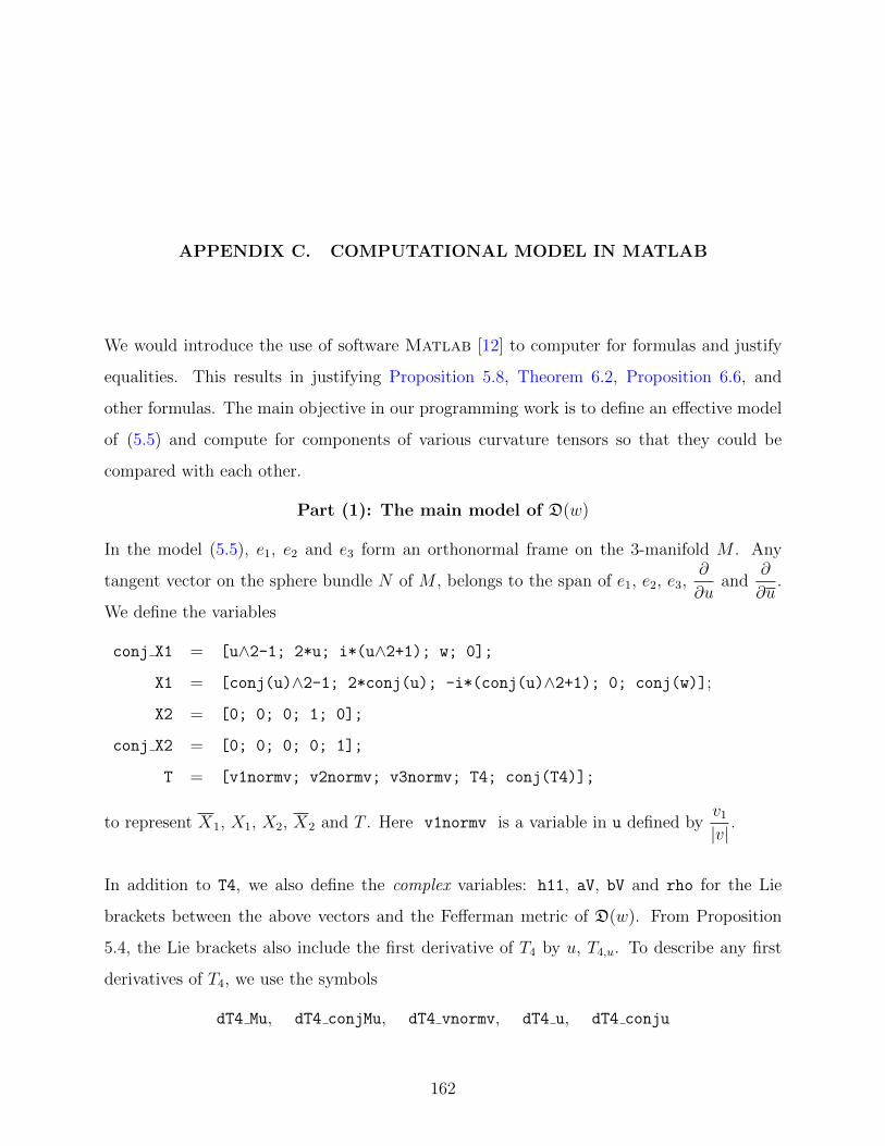
APPENDIX C. COMPUTATIONAL MODEL IN MATLAB
We would introduce the use of software Matlab [12] to computer for formulas and justify
equalities. This results in justifying Proposition 5.8, Theorem 6.2, Proposition 6.6, and
other formulas. The main objective in our programming work is to define an effective model
of (5.5) and compute for components of various curvature tensors so that they could be
compared with each other.
Part (1): The main model of D(w)
In the model (5.5), e1, e2 and e3 form an orthonormal frame on the 3-manifold M . Any
tangent vector on the sphere bundle N of M , belongs to the span of e1, e2, e3,∂
∂uand
∂
∂u.
We define the variables
conj X1 = [u∧2-1; 2*u; i*(u∧2+1); w; 0];
X1 = [conj(u)∧2-1; 2*conj(u); -i*(conj(u)∧2+1); 0; conj(w)];
X2 = [0; 0; 0; 1; 0];
conj X2 = [0; 0; 0; 0; 1];
T = [v1normv; v2normv; v3normv; T4; conj(T4)];
to represent X1, X1, X2, X2 and T . Here v1normv is a variable in u defined byv1
|v|.
In addition to T4, we also define the complex variables: h11, aV, bV and rho for the Lie
brackets between the above vectors and the Fefferman metric of D(w). From Proposition
5.4, the Lie brackets also include the first derivative of T4 by u, T4,u. To describe any first
derivatives of T4, we use the symbols
dT4 Mu, dT4 conjMu, dT4 vnormv, dT4 u, dT4 conju
162

to represent DµT4, DµT4, D v|v|T4, T4,u and T4,u respectively. Similar definition holds
for the first derivatives of h11, aV, bV and rho. Regarding the second derivatives of T4, we
create the following representation:
DµDµT4 : d2T4 MuMu, DµDµT4 : d2T4 MuconjMu, D v|v|DµT4 : d2T4 Muvnormv,
DµDµT4 : d2T4 conjMuconjMu, D v|v|DµT4 : d2T4 conjMuvnormv,
D v|v|D v
|v|T4 : d2T4 vnormvvnormv, DµDuT4 : d2T4 uMu,
DµDuT4 : d2T4 uconjMu, D v|v|DuT4 : d2T4 uvnormv,
DµDuT4 : d2T4 uMu, DµDuT4 : d2T4 uconjMu, D v|v|DuT4 : d2T4 uvnormv,
DuDuT4 : d2T4 uu, DuDuT4 : d2T4 uconju, DuDuT4 : d2T4 conjuconju.
Note that DYDX(f) = DXDY (f) + [Y,X](f), so we have
DµDµT4 = DµDµT4 +[µ, µ
](T4) = DµDµT4 + aM DµT4 − aMDµT4 + 2i h11D v
|v|T4.
In order to obtain the rest of the second derivatives of T4, we describe the vectors
[µ, µ
],[µ,
v
|v|
],[µ,
∂
∂u
]and
[ v|v|,∂
∂u
](Chapter 5) under the basis
µ, µ,
v
|v|
.
lie Mu conjMu = [aM; -conj(aM); 2*i*h11];
lie Mu vnormv = [aV; bV; 2*T4];
lie Mu ddu = [-2*conj(u)/(1+u*conj(u)); 0; -2];
lie conjMu vnormv = [conj(bV); conj(aV); 2*conj(T4)];
lie conjMu ddconju = [0; -2*u/(1+u*conj(u)); -2];
lie vnormv ddu = [0; 1/(1+u*conj(u))∧2; 0];
lie vnormv ddconju = [1/(1+u*conj(u))∧2; 0; 0];
163

Moreover, we let dT4row = [dT4 Mu, dT4 conjMu, dT4 vnormv]. Therefore, we get to
d2T4 conjMuMu = d2T4 MuconjMu + dT4row*lie Mu conjMu;
d2T4 vnormvMu = d2T4 Muvnormv + dT4row*lie Mu vnormv;
d2T4 vnormvconjMu = d2T4 conjMuvnormv + dT4row*lie conjMu vnormv;
d2T4 Muu = d2T4 uMu - dT4row*lie Mu ddu;
d2T4 conjMuu = d2T4 uconjMu;
d2T4 vnormvu = d2T4 uvnormv - dT4row*lie vnormv ddu;
d2T4 Muconju = d2T4 conjuMu;
d2T4 conjMuconju = d2T4 conjuconjMu - dT4row*lie conjMu ddconju;
d2T4 vnormvconju = d2T4 conjuvnormv - dT4row*lie vnormv ddconju;
d2T4 conjuu = d2T4 uconju;
The Fefferman metric F on C(N) (Section 5.5) is represented by the matrix F0, which
corresponds to the basisX1, X1, X2, X2, T,
∂∂γ
. We set:
F T T = -1/24*rho + i/2*(-conj(aV)+2*u*conj(T4)/(1+u*conj(u))-dT4 u);
F X1 T = i/4*(conj(dw u)- 2*u/(1+u*conj(u))*conj(w)-2*conj(T4)+aM);
F X2 T = -i*conj(u)/(2*(1+u*conj(u))); ,
F0 = [ 0, h11, 0, -i, F X1 T, 0;
h11, 0, i, 0, conj(F X1 T), 0;
0, i, 0, 0, F X2 T, 0;
-i, 0, 0, 0, conj(F X2 T), 0;
F X1 T, conj(F X1 T), F X2 T, conj(F X2 T), F T T, 1/4;
0, 0, 0, 0, 1/4, 0 ]; .
Under our convention that u1 = X1, u2 = X1, u3 = X2, u4 = X2, u5 = T and u6 = ∂∂γ
, the
Lie brackets between uj’s are expressed in the same basis of F0. We let
lieTwo = cell(6,6);
such that lieTwoj,k represents the vector [uj, uk]. For example, [u1, u2] is denoted by
164

lieTwo1,2 = [conj(aM); -aM; aM*w + 2*i*h11*T4 + dw conjMu;
-conj(aM)*conj(w) + 2*i*h11*conj(T4) - conj(dw conjMu);
-2*i*h11; 0];
according to Proposition 5.4.
The Christoffel symbols Γkij, defined by ∇uiuj = Γkij uk and found by (1.8), are the very first
things to compute for. In particular, we differentiate every Fij = F (ui, uj) by some uk. The
matrix F0 consists of variables in
CVarMain2 = [u, w, h11, T4, aM, aV, rho, dw u, dT4 u].
A particular function in Matlab is created to help finding DµFij, DµFij, D v|v|Fij, DuFij
and DuFij. The main tool is to use the chain rule, for example
DµF =
n1∑i=j
(∂F∂zj
Dµzj
)+
n1∑i=j
(∂F∂zj
(Dµzj)), (C1)
where z1, z2, · · · , zn1 are elements in CVarMain2. For the first term, Fzj or Fzj , we modify
the default function diff so that complex differentiation is executed properly.
function g = complexdiff3(f, z, s)
if isreal(z)==1
g = diff(f,z);
end
if isreal(z)==0
syms a
f1 = subs(f, abs(z), (a*z)∧(0.5));f1 = subs(f1, conj(z), a);
g1 = diff(f1, z); g1 = subs(g1, a, conj(z));
g2 = diff(f1, a); g2 = subs(g2, a, conj(z));
if s==0
g = g1;
else
g = g2;
end
end
165
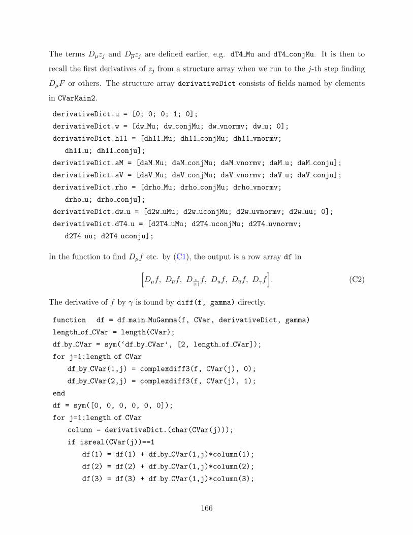
The terms Dµzj and Dµzj are defined earlier, e.g. dT4 Mu and dT4 conjMu. It is then to
recall the first derivatives of zj from a structure array when we run to the j-th step finding
DµF or others. The structure array derivativeDict consists of fields named by elements
in CVarMain2.
derivativeDict.u = [0; 0; 0; 1; 0];
derivativeDict.w = [dw Mu; dw conjMu; dw vnormv; dw u; 0];
derivativeDict.h11 = [dh11 Mu; dh11 conjMu; dh11 vnormv;
dh11 u; dh11 conju];
derivativeDict.aM = [daM Mu; daM conjMu; daM vnormv; daM u; daM conju];
derivativeDict.aV = [daV Mu; daV conjMu; daV vnormv; daV u; daV conju];
derivativeDict.rho = [drho Mu; drho conjMu; drho vnormv;
drho u; drho conju];
derivativeDict.dw u = [d2w uMu; d2w uconjMu; d2w uvnormv; d2w uu; 0];
derivativeDict.dT4 u = [d2T4 uMu; d2T4 uconjMu; d2T4 uvnormv;
d2T4 uu; d2T4 uconju];
In the function to find Dµf etc. by (C1), the output is a row array df in[Dµf, Dµf, D v
|v|f, Duf, Duf, Dγf
]. (C2)
The derivative of f by γ is found by diff(f, gamma) directly.
function df = df main MuGamma(f, CVar, derivativeDict, gamma)
length of CVar = length(CVar);
df by CVar = sym(‘df by CVar’, [2, length of CVar]);
for j=1:length of CVar
df by CVar(1,j) = complexdiff3(f, CVar(j), 0);
df by CVar(2,j) = complexdiff3(f, CVar(j), 1);
end
df = sym([0, 0, 0, 0, 0, 0]);
for j=1:length of CVar
column = derivativeDict.(char(CVar(j)));
if isreal(CVar(j))==1
df(1) = df(1) + df by CVar(1,j)*column(1);
df(2) = df(2) + df by CVar(1,j)*column(2);
df(3) = df(3) + df by CVar(1,j)*column(3);
166

df(4) = df(4) + df by CVar(1,j)*column(4);
df(5) = df(5) + df by CVar(1,j)*column(5);
else
df(1) = df(1) + df by CVar(1,j)*column(1)...
+ df by CVar(2,j)*conj(column(2));
df(2) = df(2) + df by CVar(1,j)*column(2)...
+ df by CVar(2,j)*conj(column(1));
df(1) = df(3) + df by CVar(1,j)*column(3)...
+ df by CVar(2,j)*conj(column(3));
df(1) = df(4) + df by CVar(1,j)*column(4)...
+ df by CVar(2,j)*conj(column(5));
df(1) = df(5) + df by CVar(1,j)*column(5)...
+ df by CVar(2,j)*conj(column(4));
end
end
df(6) = diff(f, gamma);
To find the values of df(uj), we also define a matrix Uvector of column vectors being uj’s.
Uvector = [0, 1, 0, 0, 0, 0;
1, 0, 0, 0, 0, 0;
0, 0, 0, 0, 1, 0;
0, w, 1, 0, T4, 0;
conj(w), 0, 0, 1, conj(T4), 0;
0, 0, 0, 0, 0, 1];
Let RGamma be a symbolic array such that RGamma(m,n,k) represents Γkmn. We first find out
Γmn,k denoted by RGamma0(m,n,k). Then, we apply Γkmn = Γmn,l Fkl.
for m=1:6
for n=1:6
for k=1:6
part1 = dF0n,k*Uvector(:,m) - dF0m,n*Uvector(:,k) ...
+ dF0m,k*Uvector(:,n);part2 = 0;
167

for ll=1:6
part2 = part2 - F0(m,ll)*lieTwon,k(ll) ...
+ F0(k,ll)*lieTwom,n(ll) + F0(n,ll)*lieTwok,m(ll);end
RGamma0(m,n,k) = 1/2*(part1+ part2);
end
end
end
The next step will be to compute for the Riemann tensor of ∇. We will follow the same
approach but now it involves more complex variables in the CVar-array. By (1.9) and (1.10),
we need to differentiate Γkij’s. The Christoffel symbols contain the following variables in
CVarMain3.
CVarMain3 = [u, w, h11, T4, aM, aV, bV, rho, ...
dw u, dw Mu, dw conjMu, dw vnormv, dh11 u, dh11 conju, dh11 Mu, ...
dh11 conjMu, dh11 vnormv, dT4 u, dT4 conju, dT4 Mu, dT4 conjMu, ...
dT4 vnormv, daM u, daM conju, daM Mu, daM conjMu, daM vnormv, ...
daV u, daV conju, daV Mu, daV conjMu, daV vnormv, ...
drho u, drho conju, drho Mu, drho conjMu, drho vnormv, ...
d2w uu, d2w uMu, d2w uconjMu, d2w uvnormv, ...
d2T4 uu, d2T4 uconju, d2T4 uMu, d2T4 uconjMu, d2T4 uvnormv];
Therefore, we have to define the second and third derivatives of variables, and expand the
structure array derivativeDict. For example, the second derivatives of T4,u include
d3T4 uMuMu, d3T4 uMuconjMu, d3T4 uMuvnormv, d3T4 uconjMuconjMu,
d3T4 uconjMuvnormv, d3T4 uvnormvvnormv, d3T4 uuMu, d3T4 uuconjMu,
d3T4 uuvnormv, d3T4 uconjuMu, d3T4 uconjuconjMu, d3T4 uconjuvnormv,
d3T4 uuu, d3T4 uuconju, d3T4 uconjuconju.
168

Other third derivatives of T4 in the form of T4,uxx can be found by the identity
DYDX(T4,u) = DXDY (T4,u) + [Y,X](T4,u).
We denote Rlmnk (1.9) by RiemCurv0(m,n,k,ll) and Rmnkl (1.10) by RiemCurv(m,n,k,ll).
The main code to find RiemCurv0(m,n,k,ll) is:
...
part1 = dRGamman,k,ll*Uvector(:,m) - dRGammam,k,ll*Uvector(:,n);part2 = 0;
for p = 1:6
part2 = part2 + RGamma(n,k,p)*RGamma(m,p,ll) ...
-RGamma(m,k,p)*RGamma(n,p,ll) -lieTwom,n(p)*RGamma(p,k,ll);end
RiemCurv0(m,n,k,ll) = part1 + part2;
...
.
Here, dRGamman,k,ll consists of the directional derivatives of Γlnk in the format of (C2).
Both the Ricci tensor, the scalar curvature and the Weyl tensor can be found directly from
RiemCurv, according to (1.11), (1.12) and (1.16) respectively.
Rij = Ric(ui, uj) : RicCurv(ii,j)
S = Rij Fij : S
Wijkl = W(ui, uj, uk, ul) : Weyl(ii,j,k,ll)
At the end of our main program, we try simplifying the components of curvature tensors
based on the Matlab function simplify. We would use an original function in order to get
rid of any ‘abs(VARIABLE)’ in the simplified expression.
function g = complex simple3(f, MVar)
MVar1=[ ];
for j=1:length(MVar)
count = has(f, MVar(j)) + has( f, conj(MVar(j)) );
if count>0
MVar1=cat(2,MVar1,MVar(j));
end
end
169
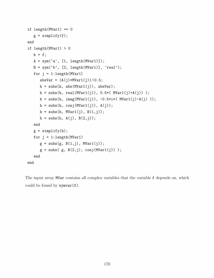
if length(MVar1) == 0
g = simplify(f);
end
if length(MVar1) > 0
h = f;
A = sym(‘a’, [1, length(MVar1)]);
B = sym(‘b’, [2, length(MVar1)], ‘real’);
for j = 1:length(MVar1)
absVar = (A(j)*MVar1(j))∧0.5;h = subs(h, abs(MVar1(j)), absVar);
h = subs(h, real(MVar1(j)), 0.5*( MVar1(j)+A(j)) );
h = subs(h, imag(MVar1(j)), -0.5*i*( MVar1(j)-A(j) ));
h = subs(h, conj(MVar1(j)), A(j));
h = subs(h, MVar1(j), B(1,j));
h = subs(h, A(j), B(2,j));
end
g = simplify(h);
for j = 1:length(MVar1)
g = subs(g, B(1,j), MVar1(j));
g = subs( g, B(2,j), conj(MVar1(j)) );
end
end
The input array MVar contains all complex variables that the variable f depends on, which
could be found by symvar(f).
170
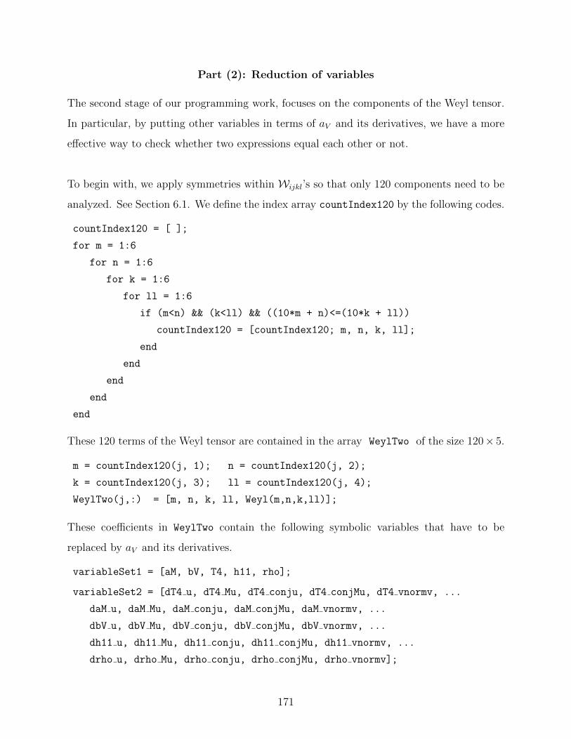
Part (2): Reduction of variables
The second stage of our programming work, focuses on the components of the Weyl tensor.
In particular, by putting other variables in terms of aV and its derivatives, we have a more
effective way to check whether two expressions equal each other or not.
To begin with, we apply symmetries within Wijkl’s so that only 120 components need to be
analyzed. See Section 6.1. We define the index array countIndex120 by the following codes.
countIndex120 = [ ];
for m = 1:6
for n = 1:6
for k = 1:6
for ll = 1:6
if (m<n) && (k<ll) && ((10*m + n)<=(10*k + ll))
countIndex120 = [countIndex120; m, n, k, ll];
end
end
end
end
end
These 120 terms of the Weyl tensor are contained in the array WeylTwo of the size 120× 5.
m = countIndex120(j, 1); n = countIndex120(j, 2);
k = countIndex120(j, 3); ll = countIndex120(j, 4);
WeylTwo(j,:) = [m, n, k, ll, Weyl(m,n,k,ll)];
These coefficients in WeylTwo contain the following symbolic variables that have to be
replaced by aV and its derivatives.
variableSet1 = [aM, bV, T4, h11, rho];
variableSet2 = [dT4 u, dT4 Mu, dT4 conju, dT4 conjMu, dT4 vnormv, ...
daM u, daM Mu, daM conju, daM conjMu, daM vnormv, ...
dbV u, dbV Mu, dbV conju, dbV conjMu, dbV vnormv, ...
dh11 u, dh11 Mu, dh11 conju, dh11 conjMu, dh11 vnormv, ...
drho u, drho Mu, drho conju, drho conjMu, drho vnormv];
171

variableSet3 = [d2T4 uu, d2T4 uMu, d2T4 MuMu, d2T4 uconju, ...
d2T4 conjuMu, d2T4 uconjMu, d2T4 uvnormv, d2T4 MuconjMu, ...
d2T4 Muvnormv, d2T4 conjuconju, d2T4 conjuconjMu, d2T4 conjuvnormv, ...
d2T4 conjMuconjMu, d2T4 conjMuvnormv, d2aM uu, d2aM uMu, d2aM MuMu, ...
d2aM uconju, d2aM conjuMu, d2aM uconjMu, d2aM uvnormv, ...
d2aM MuconjMu, d2aM Muvnormv, d2aM conjuconju, ...
d2aM conjuconjMu, d2aM conjuvnormv, d2aM conjMuvnormv, ...
d2h11 uu, d2h11 uMu, d2h11 uconju, d2h11 conjuMu, d2h11 uconjMu, ...
d2h11 uvnormv, d2h11 MuconjMu, d2h11 Muvnormv, d2h11 conjuconju, ...
d2h11 conjuconjMu, d2h11 conjuvnormv, d2h11 conjMuvnormv, ...
d2h11 vnormvvnormv, d2rho uu, d2rho uMu, d2rho MuMu, d2rho uconju, ...
d2rho conjuMu, d2rho uconjMu, d2rho MuconjMu, d2rho conjuconju, ...
d2rho conjuconjMu, d2rho conjMuconjMu];
variableSet4 = [d3T4 uuu, d3T4 uuMu, d3T4 uMuMu, d3T4 uuconju, ...
d3T4 uconjuMu, d3T4 uuconjMu, d3T4 uMuconjMu, d3T4 uconjuconju, ...
d3T4 uconjuconjMu, d3T4 uconjMuconjMu];
We would first replace the simplest variables aM , T4, bV , h11, ρ by aV and its derivatives.
aMSub = -(1+u*conj(u))∧2*daV u;
T4Sub = ((1+u*conj(u))∧2/2)*daV conju;
bVSub = u*(1+u*conj(u))*conj(daV u) + (1+u*conj(u))∧2/2*conj(d2aV uu);
h11Sub = i*(1+u*conj(u))∧2*aV + (i/2)*(1+u*conj(u))∧4*d2aV uconju;
phiW = d2w uu - 6*conj(u)/(1+u*conj(u))*dw u
+ 12*conj(u)∧2/(1+u*conj(u))∧2*w;
rhoSub = i*(phiW-conj(phiW)) + 16*theta + 12*i*(aV-conj(aV));
For the substitution of derivatives of aM , T4, bV , h11 and ρ, we find their values in terms of
aV and its derivatives by the function df main MuGamma . The CVar-set is taken to be:
172
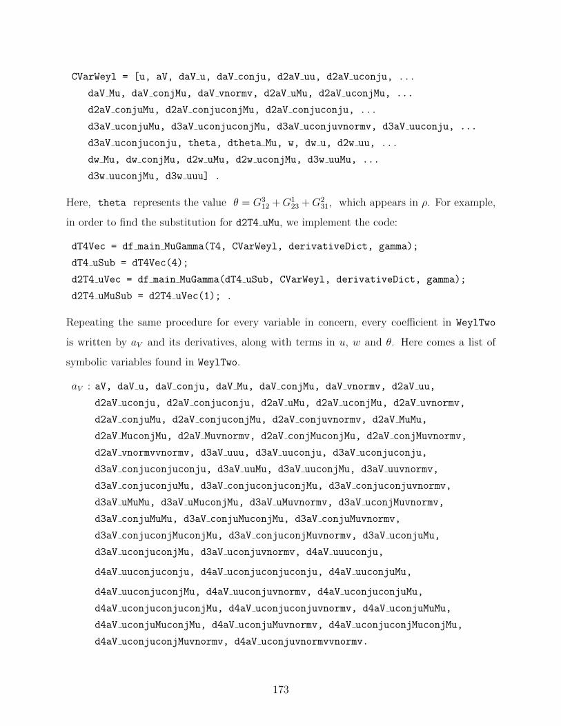
CVarWeyl = [u, aV, daV u, daV conju, d2aV uu, d2aV uconju, ...
daV Mu, daV conjMu, daV vnormv, d2aV uMu, d2aV uconjMu, ...
d2aV conjuMu, d2aV conjuconjMu, d2aV conjuconju, ...
d3aV uconjuMu, d3aV uconjuconjMu, d3aV uconjuvnormv, d3aV uuconju, ...
d3aV uconjuconju, theta, dtheta Mu, w, dw u, d2w uu, ...
dw Mu, dw conjMu, d2w uMu, d2w uconjMu, d3w uuMu, ...
d3w uuconjMu, d3w uuu] .
Here, theta represents the value θ = G312 +G1
23 +G231, which appears in ρ. For example,
in order to find the substitution for d2T4 uMu, we implement the code:
dT4Vec = df main MuGamma(T4, CVarWeyl, derivativeDict, gamma);
dT4 uSub = dT4Vec(4);
d2T4 uVec = df main MuGamma(dT4 uSub, CVarWeyl, derivativeDict, gamma);
d2T4 uMuSub = d2T4 uVec(1); .
Repeating the same procedure for every variable in concern, every coefficient in WeylTwo
is written by aV and its derivatives, along with terms in u, w and θ. Here comes a list of
symbolic variables found in WeylTwo.
aV : aV, daV u, daV conju, daV Mu, daV conjMu, daV vnormv, d2aV uu,
d2aV uconju, d2aV conjuconju, d2aV uMu, d2aV uconjMu, d2aV uvnormv,
d2aV conjuMu, d2aV conjuconjMu, d2aV conjuvnormv, d2aV MuMu,
d2aV MuconjMu, d2aV Muvnormv, d2aV conjMuconjMu, d2aV conjMuvnormv,
d2aV vnormvvnormv, d3aV uuu, d3aV uuconju, d3aV uconjuconju,
d3aV conjuconjuconju, d3aV uuMu, d3aV uuconjMu, d3aV uuvnormv,
d3aV conjuconjuMu, d3aV conjuconjuconjMu, d3aV conjuconjuvnormv,
d3aV uMuMu, d3aV uMuconjMu, d3aV uMuvnormv, d3aV uconjMuvnormv,
d3aV conjuMuMu, d3aV conjuMuconjMu, d3aV conjuMuvnormv,
d3aV conjuconjMuconjMu, d3aV conjuconjMuvnormv, d3aV uconjuMu,
d3aV uconjuconjMu, d3aV uconjuvnormv, d4aV uuuconju,
d4aV uuconjuconju, d4aV uconjuconjuconju, d4aV uuconjuMu,
d4aV uuconjuconjMu, d4aV uuconjuvnormv, d4aV uconjuconjuMu,
d4aV uconjuconjuconjMu, d4aV uconjuconjuvnormv, d4aV uconjuMuMu,
d4aV uconjuMuconjMu, d4aV uconjuMuvnormv, d4aV uconjuconjMuconjMu,
d4aV uconjuconjMuvnormv, d4aV uconjuvnormvvnormv.
173

w: u, w, dw u, dw Mu, dw conjMu, dw vnormv, d2w uu, d2w uMu, d2w uconjMu,
d2w uvnormv, d2w MuMu, d2w MuconjMu, d2w Muvnormv, d2w conjMuconjMu,
d2w conjMuvnormv, d2w vnormvvnormv, d3w uuu, d3w uuMu, d3w uuconjMu,
d3w uuvnormv, d3w uMuMu, d3w uMuconjMu, d3w uMuvnormv,
d3w uconjMuconjMu, d3w uconjMuvnormv, d4w uuuu, d4w uuuMu,
d4w uuuconjMu, d4w uuMuMu, d4w uuMuconjMu, d4w uuconjMuconjMu.
θ : theta, dtheta Mu, dtheta vnormv, d2theta MuMu, d2theta MuconjMu.
It is possible to reduce the amount of variables in WeylTwo further using differential relations
among aV and its u- or u-derivatives. Proposition 5.3 provides us with the reduction formulas
of aV,uu, aV,u u and aV,uuu. Therefore, we set
d2aV conjuconjuR = - (2*u/(1+u*conj(u)))*(daV conju +conj(daV u)) ...
- conj(d2aV uu);
d2aV uconjuR = (2/(1+u*conj(u))∧2)*(2*i*theta+conj(aV)-2*aV);
d3aV uuuR = (-6*conj(u)∧2/(1+u*conj(u))∧2)*daV u ...
- (6*conj(u)/(1+u*conj(u)))*d2aV uu;
d3aV uuconjuR = - 4*conj(u)/(1+u*conj(u))∧3*(2*i*theta+conj(aV)-2*aV) ...
+ 2/(1+u*conj(u))∧2*(-2*daV u + conj(daV conju)); .
All derivatives of aV with a u-u-derivative, two u-derivatives, or three u-derivatives, can be
substituted with other aV -terms. They are:
d2aV conjuconju, d2aV uconju, d3aV uuu, d3aV uuconju,
d3aV conjuconjuMu, d3aV conjuconjuconjMu, d3aV conjuconjuvnormv,
d3aV conjuconjuconju, d3aV uconjuMu, d3aV uconjuconjMu, d3aV uconjuvnormv,
d3aV uconjuconju, d4aV uuconjuMu, d4aV uuconjuconjMu,
d4aV uuconjuvnormv, d4aV uuconjuconju, d4aV uuuconju, d4aV uconjuMuMu,
d4aV uconjuMuconjMu, d4aV uconjuMuvnormv, d4aV uconjuconjMuconjMu,
d4aV uconjuconjMuvnormv, d4aV uconjuconjuMu, d4aV uconjuconjuconjMu,
d4aV uconjuconjuconju, d4aV uconjuconjuvnormv, d4aV uconjuvnormvvnormv.
174

We would make use of the function df main MuGamma again to replace the above variables.
The CVar-array in use is defined by
CVarWeylTwo = [u, theta, aV, daV u, daV conju, d2aV uu, daV Mu, ...
daV conjMu, daV vnormv, dtheta Mu, dtheta vnormv];
derivativeDict has already contained the fields of daV u and daV conju. We have to
modify these existing fields as well as to add fields to derivativeDict. For example,
derivativeDict.daV u = [d2aV uMu; d2aV uconjMu; d2aV uvnormv;
d2aV uu; d2aV uconjuR];
derivativeDict.daV conju = [d2aV conjuMu; d2aV conjuconjMu;
d2aV conjuvnormv; d2aV uconjuR; d2aV conjuconjuR];
derivariveDict.d2aV uu = [d3aV uuMu; d3aV uuconjMu; d3aV uuvnormv;
d3aV uuuR; d3aV uuconjuR];
If we want to replace d4aV uconjuMuMu by the new variable d4aV uconjuMuMuR, we may
implement the code:
d3aV uconjuVec = df main MuGamma(d2aV uconjuR, ...
CVarWeylTwo, derivativeDict, gamma);
d3aV uconjuMuR = d3aV uconjuVec(1);
d4aV uconjuMuVec = df main MuGamma(d3aV uconjuMuR, ...
CVarWeylTwo, derivativeDict, gamma);
d4aV uconjuMuMuR = d4aV uconjuMuVec(1); .
We mentioned in (5.18) that the following expression is real-valued:
DµDuaV − (1 + |u|2)2 aV,u aV,u − 2D v|v|aV + 2iD v
|v|θ + 4i θ aV + 2a2
V .
In some cases, we may also need to substitute (DµDuaV ) accordingly to reduce the running
time of the Matlab program.
conj d2aV conjuconjMuSub = d2aV conjuconjMu ...
- (1+u*conj(u))∧2*(daV u*daV conju) ...
+ (1+u*conj(u))∧2*conj(daV u)*conj(daV conju) - 2*daV vnormv ...
+ 2*conj(daV vnormv) + 4*i*dtheta vnormv + 4*i*theta*(aV+conj(aV)) ...
+ 2*conj(aV)∧2 - 2*aV∧2;
175
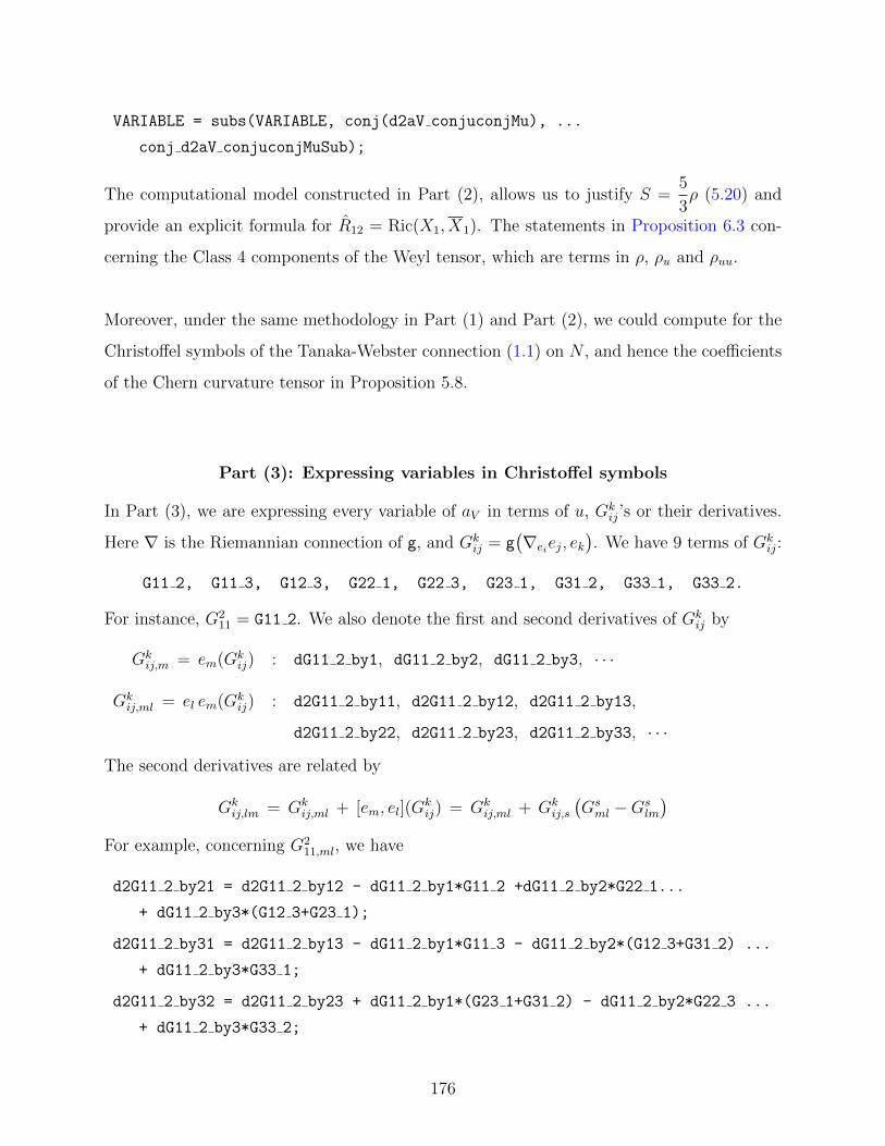
VARIABLE = subs(VARIABLE, conj(d2aV conjuconjMu), ...
conj d2aV conjuconjMuSub);
The computational model constructed in Part (2), allows us to justify S =5
3ρ (5.20) and
provide an explicit formula for R12 = Ric(X1, X1). The statements in Proposition 6.3 con-
cerning the Class 4 components of the Weyl tensor, which are terms in ρ, ρu and ρuu.
Moreover, under the same methodology in Part (1) and Part (2), we could compute for the
Christoffel symbols of the Tanaka-Webster connection (1.1) on N , and hence the coefficients
of the Chern curvature tensor in Proposition 5.8.
Part (3): Expressing variables in Christoffel symbols
In Part (3), we are expressing every variable of aV in terms of u, Gkij’s or their derivatives.
Here ∇ is the Riemannian connection of g, and Gkij = g
(∇eiej, ek
). We have 9 terms of Gk
ij:
G11 2, G11 3, G12 3, G22 1, G22 3, G23 1, G31 2, G33 1, G33 2.
For instance, G211 = G11 2. We also denote the first and second derivatives of Gk
ij by
Gkij,m = em(Gk
ij) : dG11 2 by1, dG11 2 by2, dG11 2 by3, · · ·
Gkij,ml = el em(Gk
ij) : d2G11 2 by11, d2G11 2 by12, d2G11 2 by13,
d2G11 2 by22, d2G11 2 by23, d2G11 2 by33, · · ·
The second derivatives are related by
Gkij,lm = Gk
ij,ml + [em, el](Gkij) = Gk
ij,ml + Gkij,s
(Gsml −Gs
lm
)For example, concerning G2
11,ml, we have
d2G11 2 by21 = d2G11 2 by12 - dG11 2 by1*G11 2 +dG11 2 by2*G22 1...
+ dG11 2 by3*(G12 3+G23 1);
d2G11 2 by31 = d2G11 2 by13 - dG11 2 by1*G11 3 - dG11 2 by2*(G12 3+G31 2) ...
+ dG11 2 by3*G33 1;
d2G11 2 by32 = d2G11 2 by23 + dG11 2 by1*(G23 1+G31 2) - dG11 2 by2*G22 3 ...
+ dG11 2 by3*G33 2;
176

Let RM be the Riemann tensor of ∇ with Rijkl = g(RM(ei, ej)ek, el
). So we obtain six terms
of Rijkl’s: R1212, R1213, R1223, R1313, R1323 and R2323. By definition,
R1212 = −G122,1 −G2
11,2 +G312G
123 +G3
11G322 −G1
23G231 −G3
12G231 + (G1
22)2 + (G211)2,
R1213 = −G123,1 −G3
11,2 −G122G
312 −G2
11G322 +G1
22G123 +G1
23G133 +G2
11G311 +G3
12G133,
R1223 = G322,1 −G3
12,2 +G122G
311 +G1
23G233 +G2
11G312 +G3
12G233 −G2
11G123 −G1
22G322,
R1313 = −G133,1 −G3
11,3 +G231G
312 +G2
11G233 −G2
31G123 −G3
12G123 + (G3
11)2 + (G133)2,
R1323 = −G233,1 −G3
12,3 +G231G
322 +G1
33G233 +G3
11G312 +G3
12G322 −G2
31G311 −G2
11G133,
R2323 = −G233,2 −G3
22,3 +G231G
123 +G1
22G133 −G2
31G312 −G1
23G312 + (G3
22)2 + (G233)2.
In three dimension, the first Bianchi identity of RM is equivalent to the symmetries
Rijkl = −Rjikl and Rijkl = Rklij,
while the second Bianchi identity is trivial. As a result, we obtain a set of identities.
R1213 = R1312 = G231,1 −G2
11,3 +G133G
312 +G3
11G211 −G3
11G233 −G2
31G122 −G1
33G231 −G3
12G122
R1223 = R2312 = G231,2 +G1
22,3 +G133G
322 +G1
23G233 −G2
31G211 −G2
33G231 −G1
23G211 −G3
22G122
R1323 = R2313 = G123,3 −G1
33,2 +G231G
322 +G2
33G133 −G1
22G233 −G2
31G311 −G1
23G311 −G3
22G123
We may then replace some Gkij,l’s by others as follows.
G211,3 = G1
23,1 +G311,2 +G2
31,1 −G311G
233 +G2
11G322 −
(G1
22 +G133
)(G2
31 +G123
)G3
22,1 = G312,2 +G2
31,2 +G122,3 +G1
33G322 −G1
22G311 −
(G2
11 +G233
)(G2
31 +G312
)G1
23,3 = G133,2 −G2
33,1 −G312,3 −G2
11G133 +G1
22G233 +
(G3
11 +G322
)(G3
12 +G123
) (C3)
By (C3), we substitute G211,3, G3
22,1, G123,3 and the corresponding second derivatives with
other values. The following lines of code are implemented for the substitution.
dG11 2 by3Sub = dG23 1 by1 + dG11 3 by2 + dG31 2 by1 ...
- G11 3*G33 2 + G11 2*G22 3 - (G22 1+G33 1)*(G31 2+G23 1);
177

d2G11 2 by31Sub = d2G23 1 by11 + d2G11 3 by21 + d2G31 2 by11 ...
- dG11 3 by1*G33 2 - G11 3*dG33 2 by1 + dG11 2 by1*G22 3 ...
+ G11 2*dG22 3 by1 - (dG22 1 by1+dG33 1 by1)*(G31 2+G23 1) ...
- (G22 1+G33 1)*(dG31 2 by1+dG23 1 by1);
d2G11 2 by13Sub = d2G11 2 by31Sub + G11 3*dG11 2 by1 - G33 1*dG11 2 by3 ...
+ dG11 2 by2*(G12 3 + G31 2);
d2G11 2 by32Sub = d2G23 1 by12 + d2G11 3 by22 + d2G31 2 by12 ...
- dG11 3 by2*G33 2 - G11 3*dG33 2 by2 + dG11 2 by2*G22 3 ...
+ G11 2*dG22 3 by2 - (dG22 1 by2+dG33 1 by2)*(G31 2+G23 1) ...
- (G22 1+G33 1)*(dG31 2 by2+dG23 1 by2);
d2G11 2 by23Sub = d2G11 2 by32Sub + G22 3*dG11 2 by2 - G33 2*dG11 2 by3 ...
- dG11 2 by1*(G23 1 + G31 2);
d2G11 2 by33Sub = d2G23 1 by13 + d2G11 3 by23 + d2G31 2 by13 ...
- dG11 3 by3*G33 2 - G11 3*dG33 2 by3 + dG11 2 by3*G22 3 ...
+ G11 2*dG22 3 by3 - (dG22 1 by3+dG33 1 by3)*(G31 2+G23 1)
- (G22 1+G33 1)*(dG31 2 by3+dG23 1 by3);
dG22 3 by1Sub = dG12 3 by2 + dG31 2 by2 + dG22 1 by3 ...
+ G33 1*G22 3 - G22 1*G11 3 - (G11 2+G33 2)*(G31 2+G12 3);
d2G22 3 by11Sub = d2G12 3 by21 + d2G31 2 by21 + d2G22 1 by31 ...
+ dG33 1 by1*G22 3 + G33 1*dG22 3 by1 - dG22 1 by1*G11 3 ...
- G22 1*dG11 3 by1 - (dG11 2 by1+dG33 2 by1)*(G31 2+G12 3) ...
- (G11 2+G33 2)*(dG31 2 by1+dG12 3 by1);
d2G22 3 by12Sub = d2G12 3 by22 + d2G31 2 by22 + d2G22 1 by32 ...
+ dG33 1 by2*G22 3 + G33 1*dG22 3 by2 - dG22 1 by2*G11 3 ...
- G22 1*dG11 3 by2 - (dG11 2 by2+dG33 2 by2)*(G31 2+G12 3)
- (G11 2+G33 2)*(dG31 2 by2+dG12 3 by2);
d2G22 3 by13Sub = d2G12 3 by23 + d2G31 2 by23 + d2G22 1 by33 ...
+ dG33 1 by3*G22 3 + G33 1*dG22 3 by3 - dG22 1 by3*G11 3 ...
- G22 1*dG11 3 by3 - (dG11 2 by3+dG33 2 by3)*(G31 2+G12 3)
- (G11 2+G33 2)*(dG31 2 by3+dG12 3 by3);
178

dG23 1 by3Sub = dG33 1 by2 - dG33 2 by1 - dG12 3 by3 ...
- G11 2*G33 1 + G22 1*G33 2 + (G11 3+G22 3)*(G12 3+G23 1);
d2G23 1 by31Sub = d2G33 1 by21 - d2G33 2 by11 - d2G12 3 by31 ...
- dG11 2 by1*G33 1 - G11 2*dG33 1 by1 + dG22 1 by1*G33 2 ...
+ G22 1*dG33 2 by1 + (dG11 3 by1+dG22 3 by1)*(G12 3+G23 1) ...
+ (G11 3+G22 3)*(dG12 3 by1+dG23 1 by1);
d2G23 1 by13Sub = d2G23 1 by31Sub + G11 3*dG23 1 by1 - G33 1*dG23 1 by3 ...
+ dG23 1 by2*(G12 3 + G31 2);
d2G23 1 by32Sub = d2G33 1 by22 - d2G33 2 by12 - d2G12 3 by32 ...
- dG11 2 by2*G33 1 - G11 2*dG33 1 by2 + dG22 1 by2*G33 2 ...
+ G22 1*dG33 2 by2 + (dG11 3 by2+dG22 3 by2)*(G12 3+G23 1) ...
+ (G11 3+G22 3)*(dG12 3 by2+dG23 1 by2);
d2G23 1 by23Sub = d2G23 1 by32Sub + G22 3*dG23 1 by2 - G33 2*dG23 1 by3 ...
- dG23 1 by1*(G23 1 + G31 2);
d2G23 1 by33Sub = d2G33 1 by23 - d2G33 2 by13 - d2G12 3 by33 ...
- dG11 2 by3*G33 1 - G11 2*dG33 1 by3 + dG22 1 by3*G33 2 ...
+ G22 1*dG33 2 by3 + (dG11 3 by3+dG22 3 by3)*(G12 3+G23 1) ...
+ (G11 3+G22 3)*(dG12 3 by3+dG23 1 by3);
In practice, we substitute dG11 2 by3Sub for dG11 2 by3 and so on for the first derivative
terms, and d2G11 2 by13Sub for d2G11 2 by13 etc. for the second derivative terms. In
total, we are left with 24 free coefficients of Gkij,m’s and 45 of Gk
ij,ml’s. Back to aV and its
derivatives, we begin with the following substitution for aV , θ and f .
aVSub = 1/(2*(1+u*conj(u))∧2)*( i*(mu1*conj(mu1)+mu3*conj(mu3))*G23 1 ...
+ i*(mu1*conj(mu1)+mu2*conj(mu2))*G31 2 ...
+ i*(mu2*conj(mu2)+mu3*conj(mu3))*G12 3 ...
- i*conj(mu1)*mu3*G11 2 + i*conj(mu1)*mu2*G11 3 ...
+ i*conj(mu2)*mu3*G22 1 - i*conj(mu2)*mu1*G22 3 ...
+ i*conj(mu3)*mu1*G33 2 - i*conj(mu3)*mu2*G33 1 );
thetaSub = G12 3 + G23 1 + G31 2;
Here, mu1 equals u2 − 1 , mu2 equals 2u and mu3 equals i(u2 + 1) .
179
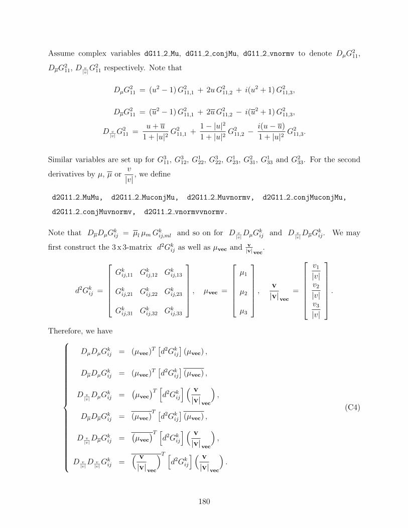
Assume complex variables dG11 2 Mu, dG11 2 conjMu, dG11 2 vnormv to denote DµG211,
DµG211, D v
|v|G2
11 respectively. Note that
DµG211 = (u2 − 1)G2
11,1 + 2uG211,2 + i(u2 + 1)G2
11,3,
DµG211 = (u2 − 1)G2
11,1 + 2uG211,2 − i(u2 + 1)G2
11,3,
D v|v|G2
11 =u+ u
1 + |u|2G2
11,1 +1− |u|2
1 + |u|2G2
11,2 −i(u− u)
1 + |u|2G2
11,3.
Similar variables are set up for G311, G3
12, G122, G3
22, G123, G2
31, G133 and G2
33. For the second
derivatives by µ, µ orv
|v|, we define
d2G11 2 MuMu, d2G11 2 MuconjMu, d2G11 2 Muvnormv, d2G11 2 conjMuconjMu,
d2G11 2 conjMuvnormv, d2G11 2 vnormvvnormv.
Note that DµDµGkij = µl µmG
kij,ml and so on for D v
|v|DµG
kij and D v
|v|DµG
kij. We may
first construct the 3 x 3-matrix d2Gkij as well as µvec and v
|v|vec.
d2Gkij =
Gkij,11 Gk
ij,12 Gkij,13
Gkij,21 Gk
ij,22 Gkij,23
Gkij,31 Gk
ij,32 Gkij,33
, µvec =
µ1
µ2
µ3
,v
|v|vec
=
v1
|v|v2
|v|v3
|v|
.
Therefore, we have
DµDµGkij = (µvec)T
[d2Gk
ij
](µvec) ,
DµDµGkij = (µvec)T
[d2Gk
ij
](µvec) ,
D v|v|DµG
kij =
(µvec
)T [d2Gk
ij
] ( v
|v|vec
),
DµDµGkij = (µvec)
T [d2Gk
ij
](µvec) ,
D v|v|DµG
kij =
(µvec
)T [d2Gk
ij
] ( v
|v|vec
),
D v|v|D v
|v|Gkij =
( v
|v|vec
)T [d2Gk
ij
] ( v
|v|vec
).
(C4)
180

To replace derivatives of aV or θ, we compute their values through the self-created Matlab
function df main MuGamma. The procedures involved include two steps: replace these terms
by directional derivatives of Gkij along µ, µ and v
|v| . Then, we replace every DµGkij, DµG
kij,
D v|v|Gkij and so on, by Gk
ij,m’s (dGij k byM) and Gkij,ml’s (d2Gij k byML).
In the first step of Part (3), he CVar-array is chosen as
CVarW72 = [ u, G12 3, G23 1, G31 2, G11 2, G11 3, G22 1, G22 3, ...
G33 1, G33 2, dG11 2 Mu, dG11 3 Mu, dG12 3 Mu, dG22 1 Mu, dG22 3 Mu, ...
dG23 1 Mu, dG31 2 Mu, dG33 1 Mu, dG33 2 Mu, ...
dG11 2 conjMu, dG11 3 conjMu, dG12 3 conjMu, dG22 1 conjMu, ...
dG22 3 conjMu, dG23 1 conjMu, dG31 2 conjMu, dG33 1 conjMu, ...
dG33 2 conjMu, dG11 2 vnormv, dG11 3 vnormv, dG12 3 vnormv, ...
dG22 1 vnormv, dG22 3 vnormv, dG23 1 vnormv, dG31 2 vnormv, ...
dG33 1 vnormv, dG33 2 vnormv];
Inside derivativeDict, for example, we create the fields:
derivativeDict.G11 2 = [dG11 2 Mu; dG11 2 conjMu; dG11 2 vnormv; 0; 0];
derivativeDict.dG11 2 Mu = [d2G11 2 MuMu; d2G11 2 MuconjMu;
d2G11 2 Muvnormv; d2G11 2 Muu; 0];
derivativeDict.dG11 2 conjMu = [d2G11 2 conjMuMu; d2G11 2 conjMuconjMu;
d2G11 2 conjMuvnormv; 0; d2G11 2 conjMuconju];
derivativeDict.dG11 2 vnormv = [d2G11 2 vnormvMu; d2G11 2 vnormvconjMu;
d2G11 2 vnormvvnormv; d2G11 2 vnormvu; d2G11 2 vnormvconju]; .
We have to replace elements of the arrays below by Gkij’s and their µ, µ or v
|v| -derivatives.
variableSetG1 = [theta, aV, daV u, daV conju, d2aV uu];
variableSetG2 = [daV Mu, daV conjMu, daV vnormv, d2aV uMu, ...
d2aV uconjMu, d2aV uvnormv, d2aV conjuMu, d2aV conjuconjMu, ...
d2aV conjuvnormv, d3aV uuMu, d3aV uuconjMu, d3aV uuvnormv, ...
dtheta Mu, dtheta vnormv];
181

variableSetG3 = [d2aV MuMu, d2aV MuconjMu, d2aV Muvnormv, ...
d2aV conjMuconjMu, d2aV conjMuvnormv, d2aV vnormvvnormv, ...
d3aV uMuMu, d3aV uMuconjMu, d3aV uMuvnormv, d3aV uconjMuconjMu, ...
d3aV uconjMuvnormv, d3aV uvnormvvnormv, d3aV conjuMuMu, ...
d3aV conjuMuconjMu, d3aV conjuMuvnormv, d3aV conjuconjMuconjMu, ...
d3aV conjuconjMuvnormv];
variableSetG4 = [d4aV uuMuMu, d4aV uuMuconjMu, d4aV uuMuvnormv, ...
d4aV uuvnormvvnormv, d4aV uuconjMuconjMu, d4aV uuconjMuvnormv, ...
d2theta MuMu, d2theta MuconjMu, d2theta Muvnormv, d2theta vnormvvnormv];
For instance, to substitute DµDµDuDuaV , we can implement these lines of code:
daVVec = df main MuGamma(aVSub, CVarW72, derivativeDict, gamma);
daV uSub = daVVec(4);
d2aV uVec = df main MuGamma(daV uSub, CVarW72, derivativeDict, gamma);
d2aV uuSub = d2aV uVec(4);
d3aV uuVec = df main MuGamma(d2aV uuSub, CVarW72, derivativeDict, gamma);
d3aV uuMuSub = d3aV uuVec(1);
d4aV uuMuVec = df main MuGamma(d3aV uuMuSub, CVarW72, ...
derivativeDict, gamma);
d4aV uuMuMuSub = d4aV uuMuVec(1);
The second step of Part (3) is a rather straightforward replacement following (C3) and (C4).
(1) Replace DµDµGkij’s and other 2nd derivatives by Gk
ij,ml’s and Gkij,m’s.
(2) Replace DµGkij, DµG
kij and D v
|v|Gkij by Gk
ij,m’s.
(3) Replace G211,13, G2
11,23, G211,33, G3
22,11, G322,12, G3
22,13, G123,13, G1
23,23 and G123,33.
(4) Replace G211,3, G3
22,1 and G123,3.
As a final remark to Part (3), it is reasonable for us to define Gkij,m and Gk
ij,ml to be real
variables. Alternatively, we may have to insert extra code, for example
VARIABLE = subs(VARIABLE, conj(dG11 2 by2), dG11 2 by2); .
182

As a primary application, we would justify the first item of Theorem 6.2 in the case of twistor
CR manifolds. The crucial step here is to showW1212 = C1111 andW1214 = C1112. We denote
W1212, W1214 by W1212, W1214, and C1111, C1112 by C1111, C1112.
temp = W1212 - C1111;
temp = subs(temp, conj(d2aV conjuconjMu), conj d2aV conjuconjMuSub);
temp = complex simple3(temp, MVAR);
...
for j = 1:length(variableSetG3)
char01 = char(variableSetG3(j));
char02 = [char01, ‘Sub’];
eval( [‘temp=subs(temp,’ , char01, ‘,’ , char02 , ’);’ ]);
end
% ( also for variableSetG2 and then variableSetG1. )
...
temp = subs(temp, d2G11 2 MuMu, transpose(muVec)*d2G11 2*muVec);
temp = subs(temp, d2G11 2 MuconjMu, ...
transpose(muVec)*d2G11 2*conj(muVec));
temp = subs(temp, d2G11 2 Muvnormv, transpose(muVec)*d2G11 2*vnormvVec);
temp = subs(temp, d2G11 2 conjMuconjMu, ...
transpose(conj(muVec))*d2G11 2*conj(muVec));
temp = subs(temp, d2G11 2 conjMuvnormv, ...
transpose(conj(muVec))*d2G11 2*vnormvVec);
temp = subs(temp, d2G11 2 vnormvvnormv, ...
transpose(vnormvVec)*d2G11 2*vnormvVec);
% ( also for other d2Gij k’s. )
...
temp = subs(temp, dG11 2 Mu, ...
mu1*dG11 2 by1 + mu2*dG11 2 by2 + mu3*dG11 2 by3);
temp = subs(temp, dG11 2 conjMu, conj(mu1)*dG11 2 by1 ...
+ conj(mu2)*dG11 2 by2 + conj(mu3)*dG11 2 by3);
temp = subs(temp, dG11 2 vnormv, ...
v1normv*dG11 2 by1 + v2normv*dG11 2 by2 + v3normv*dG11 2 by3);
% ( also for other dGij k’s. )
...
183

...
variableSetBianchi1 = [dG11 2 by3, dG22 3 by1, dG23 1 by3];
variableSetBianchi2 = [d2G11 2 by13, d2G11 2 by23, d2G11 2 by33, ...
d2G22 3 by11, d2G22 3 by12, d2G22 3 by13, ...
d2G23 1 by13, d2G23 1 by23, d2G23 1 by33];
for j=1:length(variableSetBianchi2)
char03 = char(variableSetBianchi2);
char04 = [char03, ‘Sub’];
eval( [‘temp=subs(temp,’ , char03, ‘,’ , char04 , ’);’ ]);
end
% ( also for variableSetBianchi1. )
...
Finally, we apply the function complex simple3 with MVar containing u and w-terms.
Part (4): Application to verify Proposition 6.6
As an important application of our computer model of the twistor CR structure D (of zero
torsion), we will describe how to justify Proposition 6.6 in details. At the beginning, we
have to put w = f , i.e. substitute f for w.
f = u*(1+u*conj(u))∧3*conj(daV u) + (1+u*conj(u))∧4/2*conj(d2aV uu);
Every derivative of w will be replaced by the corresponding derivative of f , including
wSet = [w, dw Mu, dw conjMu, dw vnormv, dw u, d2w uMu, d2w uconjMu, ...
d2w uvnormv, d2w uu, d2w MuMu, d2w MuconjMu, d2w Muvnormv, ...
d2w conjMuconjMu, d2w conjMuvnormv, d2w vnormvvnormv, d3w uMuMu. ...
d3w uMuconjMu, d3w uMuvnormv, d3w uconjMuconjMu, d3w uconjMuvnormv, ...
d3w uuMu, d3w uuconjMu, d3w uuvnormv, d3w uuu, d4w uuMuMu, ...
d4w uuMuconjMu, d4w uuconjMuconjMu, d4w uuuMu, d4w uuuconjMu, d4w uuuu];
The derivatives of f are found by the function df main MuGamma. The CVar array is set as
CVarW7 = [u, aV, daV u, daV conju, d2aV uu, theta, d2aV uMu, ...
d2aV uconjMu, d2aV uvnormv, d3aV uuMu, d3aV uuconjMu, d3aV uuvnormv, ...
d2aV conjuMu, d2aV conjuconjMu, daV Mu, daV conjMu, dtheta Mu]; .
184

The next step is to define variables to represent components of the Schouten tensor (P),
which are found by (6.2) and (6.3). We let P and covP be the Schouten tensor and its
covariant derivative respectively.
Pij : P(ii,j) and ∇iPjk : covP(ii,j,k)
Both P(ii,j) and covP(ii,j,k) are in terms of Gkij’s , Gk
ij,m’s and Gkij,ml’s. On the other
hand, we define another set of real variables:
covP112, covP113, covP122, covP123, covP133,
covP211, covP212, covP213, covP223, covP233,
covP311, covP312, covP313, covP322, covP323.
Let dGset be the array of every Gij k and dGij k byM, and d2Gset be that of all variables
in the form of ‘d2Gij k byML’ (Gkij,ml). Moreover, we let
covPset = [covP112, covP113, covP122, covP123, covP133, ...
covP211, covP212, covP213, covP223, covP233, ...
covP311, covP312, covP313, covP322, covP323]; .
We would replace some Gkij,ml’s by ∇iPjk, following the lines of code below.
...
indexArray = [‘‘112’’, ‘‘113’’, ‘‘122’’, ‘‘123’’, ‘‘133’’, ...
‘‘211’’, ‘‘212’’, ‘‘213’’, ‘‘223’’, ‘‘233’’, ‘‘311’’, ...
‘‘312’’, ‘‘313’’, ‘‘322’’, ‘‘323’’];
for j=1:15
char01 = char(indexArray(j));
m = str2num(char01(1));
n = str2num(char01(2));
k = str2num(char01(3));
[termVec, gVec] = coeffs(covP(m,n,k),d2Gset);
eval([‘term’ , char01 , ‘=termVec(end);’]);
end
...
185

d2G33 2 by11Sub = covP112 - d2G12 3 by13 - term112;
d2G33 2 by22Sub = d2G11 2 by22 + d2G11 3 by23 + d2G22 1 by12 ...
- d2G22 3 by23 + d2G33 1 by12 - 2*covP211 + 2*term211;
d2G31 2 by12Sub = covP113 - d2G22 1 by13 - term113;
d2G33 2 by23Sub = d2G11 2 by23Sub + d2G11 3 by33 + d2G22 1 by13 ...
- d2G22 3 by33 + d2G33 1 by13 - 2*covP311 + 2*term311;
d2G33 2 by12Sub = 2*covP122 - d2G11 2 by12 + d2G11 3 by13 ...
- d2G22 1 by11 - d2G22 3 by13Sub ...
+ d2G33 1 by11 - 2*term122;
d2G12 3 by23Sub = covP212 - d2G33 2 by12 - term212;
d2G33 1 by11Sub = covP133 + d2G11 2 by12 - d2G11 3 by13 + d2G22 1 by11 ...
-covP122 - term133 + term122;
d2G31 2 by23Sub = covP313 - d2G22 1 by33 - term313;
d2G23 1 by12Sub = covP223 - d2G11 3 by22 - term223;
d2G22 1 by13Sub = covP322 + covP311 - term311- term322- d2G11 2 by23Sub;
d2G11 3 by23Sub = covP323 - d2G23 1 by13Sub - term323;
d2G33 1 by12Sub = covP233 + covP211 - term233 - term211 - d2G11 3 by23;
d2G23 1 by11Sub = covP123 - d2G11 3 by12 - term123;
d2G31 2 by22Sub = covP213 - d2G22 1 by23 - term213;
d2G33 2 by13Sub = covP312 -d2G12 3 by33 - term312;
...
In Proposition 6.6, we interpret W1212, W1215, W1515 and W1525 as a polynomial in u and u
with coefficients being components of the Cotton tensor:
Cijk = ∇kPij −∇jPik.
Take W1212 as an example. We first find an approximation A1212 such that (W1212 −A1212)
is without any second derivatives of Gkij’s.
186
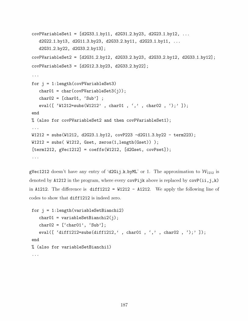
covPVariableSet1 = [d2G33 1 by11, d2G31 2 by23, d2G23 1 by12, ...
d2G22 1 by13, d2G11 3 by23, d2G33 2 by11, d2G23 1 by11, ...
d2G31 2 by22, d2G33 2 by13];
covPVariableSet2 = [d2G31 2 by12, d2G33 2 by23, d2G33 2 by12, d2G33 1 by12];
covPVariableSet3 = [d2G12 3 by23, d2G33 2 by22];
...
for j = 1:length(covPVariableSet3)
char01 = char(covPVariableSet3(j));
char02 = [char01, ‘Sub’] ;
eval([ ‘W1212=subs(W1212’ , char01 , ‘,’ , char02 , ‘);’ ]);
end
% (also for covPVariableSet2 and then covPVariableSet1);
...
W1212 = subs(W1212, d2G23 1 by12, covP223 -d2G11 3 by22 - term223);
W1212 = subs( W1212, Gset, zeros(1,length(Gset)) );
[term1212, gVec1212] = coeffs(W1212, [d2Gset, covPset]);
...
gVec1212 doesn’t have any entry of ‘d2Gij k byML’ or 1. The approximation to W1212 is
denoted by A1212 in the program, where every covPijk above is replaced by covP(ii,j,k)
in A1212. The difference is diff1212 = W1212 - A1212. We apply the following line of
codes to show that diff1212 is indeed zero.
for j = 1:length(variableSetBianchi2)
char01 = variableSetBianchi2(j);
char02 = [‘char01’, ‘Sub’];
eval([ ‘diff1212=subs(diff1212,’ , char01 , ‘,’ , char02 , ‘);’ ]);
end
% (also for variableSetBianchi1)
...
187
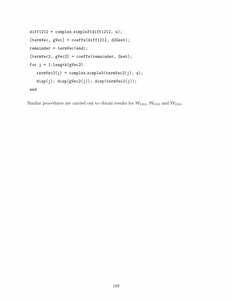
diff1212 = complex simple3(diff1212, u);
[termVec, gVec] = coeffs(diff1212, d2Gset);
remainder = termVec(end);
[termVec2, gVec2] = coeffs(remainder, Gset);
for j = 1:length(gVec2)
termVec2(j) = complex simple3(termVec2(j), u);
disp(j); disp(gVec2(j)); disp(termVec2(j));
end
Similar procedures are carried out to obtain results for W1215, W1515 and W1525.
188
BIBLIOGRAPHY
[1] B. Alexandrov & S. Ivanov, “Weyl structures with positive Ricci tensor,” Diff. Geom.Appl., vol. 18, no. 3, pp. 343-350, May 2003
[2] S. S. Chern & J. K. Moser, “Real Hypersurfaces in Complex Manifolds,” Acta Mathe-matica, vol. 133, pp. 219271, 1974.
[3] A. Boggess, CR Manifolds and the Tangential Cauchy-Riemann Complex. Boca Raton,FL: CRC Press, 1991.
[4] S. Dragomir & G. Tomassini, Differential Geometry and Analysis on CR Manifolds.Boston: Birkhauser, 2006.
[5] T. Friedrich, Dirac Operators in Riemannian Geometry. A. M. S., 2000.
[6] C. R. Graham, “On Sparling’s Characterization of Fefferman Metrics,” American J.Mathematics, vol. 109, no. 5, pp. 853-874, Oct. 1987.
[7] W. Kuhnel, Differential Geometry: Curves-Surfaces-Manifolds, 2nd ed. A.M.S., 2006.
[8] C. R. LeBrun, “Spaces of Complex Geodesics & Related Structures,” Ph.D. disserta-tion, Hertford College, Univ. of Oxford, Oxford, 1980.
[9] C. R. LeBrun, “Twistor CR Manifolds and Three-Dimensional Conformal Geometry,”Trans. A.M.S., vol. 284, no. 2, pp. 601616, 1984.
189
[10] C. R. LeBrun, “Foliated CR Manifolds,” J.Differential Geom., vol. 22, no. 1, pp. 81-96,Feb. 1985.
[11] J. M. Lee, “The Fefferman Metric and Pseudohermitian Invariants,” Trans. A.M.S.,vol. 296, no. 1, pp. 411-429, 1986.
[12] MATLAB version 9.3.0. (R2017b). Natick, Massachusetts: The MathWorks Inc., 2017.
[13] P. Nurowski & G. A. J. Sparling, “3-dimensional Cauchy-Riemann structures and 2ndorder ordinary differential equations,” Classical and Quantum Gravity, vol. 20, no.23,pp. 4995-5016, 2003.
[14] R. Penrose & M. A. H. MacCallum, “Twistor Theory: An Approach to the Quan-tization of Fields and Space-Time,” Physics Reports, vol. 6, no. 4, pp. 241-316, Jun. 1972.
[15] R. Penrose, “Physical space-time and nonrealizable CR-structures,” Bull. Amer. Math.Soc. (N.S.), vol. 8, no. 3, pp. 427-448, 1983.
[16] S. Sasaki, “On the differential geometry of tangent bundles of Riemannian manifolds,”Tohoku. Math. J. (2), vol. 10, no.3, pp. 338-354, 1958.
[17] I. L. Shapiro, “Physical Aspect of the Space-Time Torsion,” Physics Reports, vol. 357,no. 2, pp. 113-214, Jan. 2002.
[18] G. A. J. Sparling, “Twistor theory and the characterization of Fefferman’s conformalstructure,” preprint.
[19] F. W. Warner, Foundations of Differentiable Manifolds and Lie Groups. New York,NY, USA: Springer-Verlag, 1983.
[20] S. M. Webster, “Pseudo-Hermitian Structures on a Real Hypersurface,” J.DifferentialGeom., vol. 13, no. 1, pp. 25-41, 1978.
190
Related Documents