Geometry of SU(3) Manifolds · ples, I study the twistor spaces of Riemannian 4-manifolds. It turns out that twistor spaces over self-dual Einstein 4-manifolds provide admissible

Geometry of SU(3) Manifolds

by

Feng Xu

Department of MathematicsDuke University

Date:

Approved:

Robert L. Bryant, Advisor

William Allard

Hubert Bray

Mark Stern

Dissertation submitted in partial fulfillment of the requirements for the degree ofDoctor of Philosophy in the Department of Mathematics

in the Graduate School of Duke University2008

Abstract(Differential Geometry)

Geometry of SU(3) Manifolds

by

Feng Xu

Department of MathematicsDuke University

Date:

Approved:

Robert L. Bryant, Advisor

William Allard

Hubert Bray

Mark Stern

An abstract of a dissertation submitted in partial fulfillment of the requirements forthe degree of Doctor of Philosophy in the Department of Mathematics

in the Graduate School of Duke University2008

Copyright c© 2008 by Feng XuAll rights reserved

Abstract

I study the differential geometry of 6-manifolds endowed with various SU(3) struc-

tures from three perspectives. The first is special Lagrangian geometry; The second

is pseudo-Hermitian-Yang-Mills connections or, more generally, ω-anti-self dual in-

stantons; The third is pseudo-holomorphic curves.

For the first perspective, I am interested in the interplay between SU(3)-structures

and their special Lagrangian submanifolds. More precisely, I study SU(3)-structures

which locally support as ‘nice’ special Lagrangian geometry as Calabi-Yau 3-folds

do. Roughly speaking, this means that there should be a local special Lagrangian

submanifold tangent to any special Lagrangian 3-plane. I call these SU(3)-structures

admissible. By employing Cartan-Kahler machinery, I show that locally such admis-

sible SU(3)-structures are abundant and much more general than local Calabi-Yau

structures. However, the moduli space of the compact special Lagrangian subman-

ifolds is not so well-behaved in an admissible SU(3)-manifold as in the Calabi-Yau

case. For this reason, I narrow attention to nearly Calabi-Yau manifolds, for which

the special Lagrangian moduli space is smooth. I compute the local generality of

nearly Calabi-Yau structures and find that they are still much more general than

Calabi-Yau structures. I also discuss the relationship between nearly Calabi-Yau

and half-flat SU(3)-structures. To construct complete or compact admissible exam-

ples, I study the twistor spaces of Riemannian 4-manifolds. It turns out that twistor

spaces over self-dual Einstein 4-manifolds provide admissible and nearly Calabi-Yau

manifolds. I also construct some explicit special Lagrangian examples in nearly

Kahler CP3 and the twistor space of H4.

For the second perspective, we are mainly interested in pseudo-Hermitian-Yang-

iv

Mills connections on nearly Kahler six manifolds. Pseudo-Hermitian-Yang-Mills con-

nections were introduced by R. Bryant in [4] to generalize Hermitian-Yang-Mills

concept in Kahler geometry to almost complex geometry. If the SU(3)-structure is

nearly Kahler, I show that pseudo-Hermitian-Yang-Mills connections (or, more gen-

erally, ω-anti-self-dual instantons) enjoy many nice properties. For example, they

satisfy the Yang-Mills equation and thus removable singularity results hold for such

connections. Moreover, they are critical points of a Chern-Simons functional. I de-

rive a Weitzenbock formula for the deformation and discuss some of its application.

I construct some explicit examples that display interesting singularities.

For the third perspective, I study pseudo-holomorphic curves in nearly Kahler

CP3. I construct a one-to-one correspondence between null torsion curves in the

nearly Kahler CP3 and contact curves in the Kahler CP3 (considered as a complex

contact manifold). From this, I derive a Weierstrass formula for all null torsion

curves by employing a result of R. Bryant in [9]. In this way, I classify all pseudo-

holomorphic curves of genus 0.

v

Contents

Abstract iv

Acknowledgements viii

Introduction 1

0.1 SU(3)-structure on vector spaces . . . . . . . . . . . . . . . . . . . . 1

0.2 SU(3)-structures on 6-manifolds . . . . . . . . . . . . . . . . . . . . . 3

0.2.1 G-structure . . . . . . . . . . . . . . . . . . . . . . . . . . . . 3

0.2.2 SU(3)-structures . . . . . . . . . . . . . . . . . . . . . . . . . 5

1 Special Lagrangian and SU(3)-Structures 9

1.1 Special Lagrangian geometry and admissible SU(3) structures . . . . 9

1.1.1 Admissible SU(3)-structures . . . . . . . . . . . . . . . . . . . 10

1.1.2 First examples . . . . . . . . . . . . . . . . . . . . . . . . . . 12

1.1.3 Generalities . . . . . . . . . . . . . . . . . . . . . . . . . . . . 14

1.2 Examples from twistor spaces of Riemannian four-manifolds . . . . . 22

1.2.1 Four dimensional Riemannian geometry . . . . . . . . . . . . 23

1.2.2 Twistor spaces of self-dual Einstein 4-manifolds . . . . . . . . 26

1.3 Complete special Lagrangian examples . . . . . . . . . . . . . . . . . 27

1.3.1 An example in J (S4) = CP3 . . . . . . . . . . . . . . . . . . 28

1.3.2 An example in J (H4) . . . . . . . . . . . . . . . . . . . . . . 32

1.4 Compact special Lagrangian submanifolds in nearly Calabi-Yau man-ifolds . . . . . . . . . . . . . . . . . . . . . . . . . . . . . . . . . . . . 36

1.4.1 Deformations of compact special Lagrangian 3-folds . . . . . . 37

1.4.2 Obstructions to the existence of compact SL 3-folds . . . . . . 39

vi

2 Instantons on Nearly Kahler 6-Manifolds 42

2.1 Some linear algebra in 6 and 7 dimensions . . . . . . . . . . . . . . . 44

2.1.1 Dimension 6 . . . . . . . . . . . . . . . . . . . . . . . . . . . . 45

2.1.2 Dimension 7 . . . . . . . . . . . . . . . . . . . . . . . . . . . . 57

2.2 Anti-self-dual instantons on nearly Kahler 6-manifolds and G2-cones . 58

2.2.1 Nearly Kahler 6-manifolds . . . . . . . . . . . . . . . . . . . . 59

2.2.2 G2-cones over a nearly Kahler 6-manifold . . . . . . . . . . . . 61

2.2.3 ω anti-self-dual instantons . . . . . . . . . . . . . . . . . . . . 62

2.2.4 Ω-anti-self-dual instantons on the G2-cone . . . . . . . . . . . 69

2.3 A Weitzenbock formula . . . . . . . . . . . . . . . . . . . . . . . . . . 71

2.3.1 The general formula . . . . . . . . . . . . . . . . . . . . . . . 71

2.3.2 Deformation of ω-anti-self-dual instantons . . . . . . . . . . . 74

2.4 SO(4)-invariant examples . . . . . . . . . . . . . . . . . . . . . . . . 81

2.4.1 A dense open subset U of S6 . . . . . . . . . . . . . . . . . . . 82

2.4.2 Bundle constructions and SO(4)-invariant connections . . . . 83

2.4.3 SO(4)-invariant instantons . . . . . . . . . . . . . . . . . . . . 88

3 Pseudo-Holomorphic Curves in Nearly Kahler CP3 93

3.1 Structure equations, projective spaces, and the flag manifold . . . . . 93

3.2 Pseudo-holomorphic curves in CP3 . . . . . . . . . . . . . . . . . . . 98

4 Summary 106

Bibliography 107

Biography 110

vii

Acknowledgements

It is a great pleasure to thank my advisor, Robert Bryant. for spending numer-

ous hours sharing his knowledge of Differential Geometry with me. Without his

encouragements, this thesis would never have been.

I thank Mark Stern, Chad Schoen, Les Saper and many other professors at Duke

who taught me various mathematical courses. I have gained useful knowledge from

these courses toward this thesis.

I enjoyed many conversations with Shu Dai. I thank him for this and for his

help with mailing my stuffs when I was away from Duke. I thank my mathematical

brothers, Abe Smith and Conrad Hengebach for many interesting discussions both

on mathematics and on life.

I am grateful for the hospitality of MSRI and Berkeley where I have worked

during the academic year 2007-2008. Berkeley is also a great place to know many

new friends, Jia Yu and Xinwen Zhu, Liyan Lin and Guoliang Wu, Jing Xiong and

Haijian Shi and above all, my girl friend, Yun Long.

It is never forgettable that so many friends back at Duke have made Durham

life fascinating. I enjoyed many nice dinners and poker games with Shuyi Wanng,

Junjie Zhang, Huiyan Sang, Ping Zhou and Jianwei Li. I also thank Chenghui Cai

and Tingting Chen for help and encouragements to overcome much difficulty in life.

I thank Yun Long for her love and encouragement especially when I was so frus-

trated in job hunting. She has made Berkeley a home for me.

Finally, this thesis would not be possible were it not for the love and encourage-

ment provided by my parents, Shusheng Xu and Kai Zhang, and my brother Jian

Xu.

viii

Introduction

0.1 SU(3)-structure on vector spaces

Let V be a 6-dimensional vector space. Let (Ω, φ) ∈ Λ2V ∗⊕Λ3V ∗ be a pair of forms

with Ω nondegenerate. Clearly the full linear group GL(V ) acts on such pairs by

pullback. It is interesting to ask what the orbits and stabilizer groups are like. This

problem was solved first by Banos in [3]. Later on, Bryant gave a simplified proof in

[4].

There are two ways to this problem in the literature. One is to normalize Ω first

and then consider the orbits of φ under the symplectic group Sp(Ω). Note that under

the action of Sp(Ω), Λ3V ∗ decomposes into two irreducible pieces: Ω∧V ∗ and Λ30V∗

of effective forms annihilated by wedge product by Ω. Since Sp(V ) acts transitively

on V ∗ \ 0, Ω ∧ V ∗ has only two obvious orbits. The difficult part is the orbits in

Λ30V∗. This approach was adopted in [3].

The other is just the opposite, namely to classify φ orbits under GL(V ) and then

to normalize Ω under different stabilizer groups of φ. The second turns out to be

simpler and was adopted in [4]. We cite the result as follows

Proposition 0.1.1 ([3],[4]). Suppose (ω,Ψ) ∈ Λ2V ∗ ⊕ Λ3V ∗. Assume ω is nonde-

generate and Ψ is primitive (i.e., ω ∧Ψ = 0). Then under the action of GL(V ), the

pair (ω, φ) can be normalized to one of the following with the corresponding stabilizer

group G(Ω, φ):

1

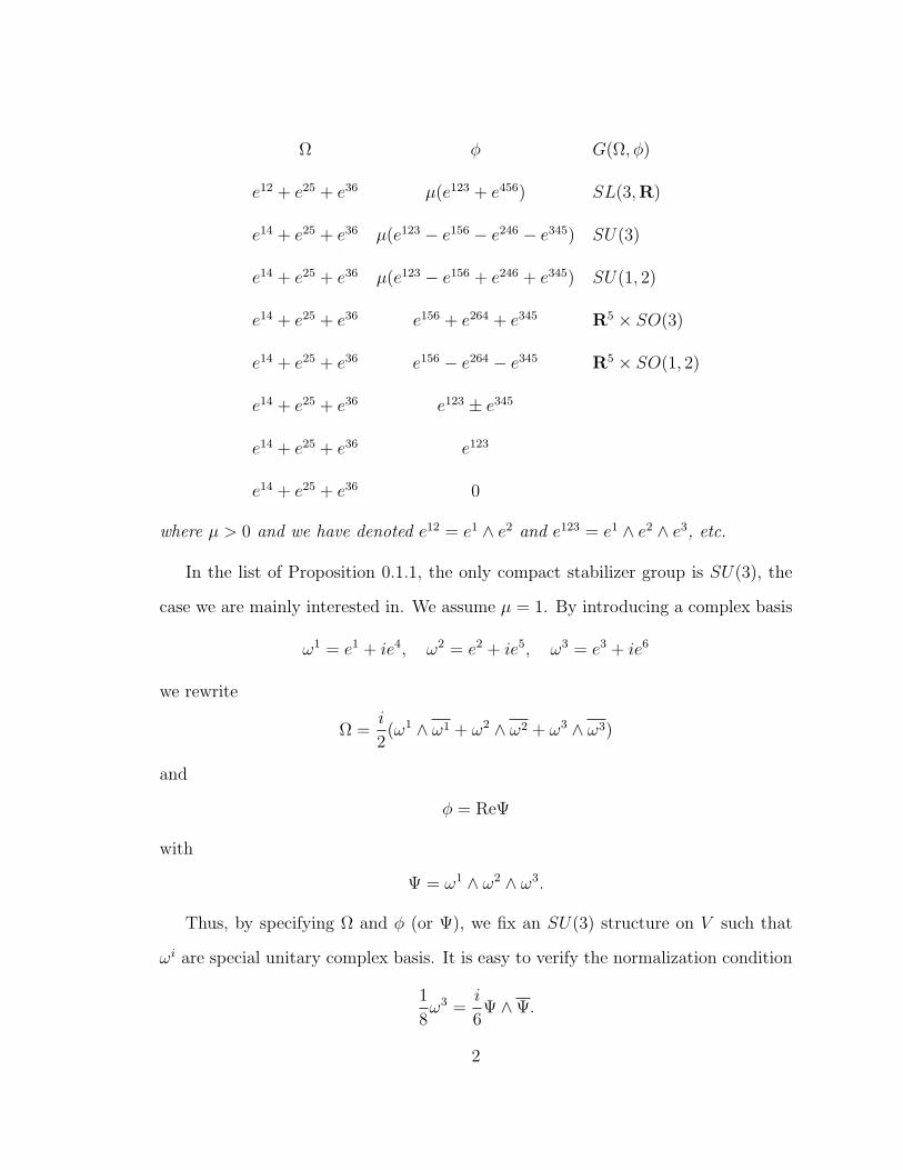
Ω φ G(Ω, φ)

e12 + e25 + e36 µ(e123 + e456) SL(3,R)

e14 + e25 + e36 µ(e123 − e156 − e246 − e345) SU(3)

e14 + e25 + e36 µ(e123 − e156 + e246 + e345) SU(1, 2)

e14 + e25 + e36 e156 + e264 + e345 R5 × SO(3)

e14 + e25 + e36 e156 − e264 − e345 R5 × SO(1, 2)

e14 + e25 + e36 e123 ± e345

e14 + e25 + e36 e123

e14 + e25 + e36 0

where µ > 0 and we have denoted e12 = e1 ∧ e2 and e123 = e1 ∧ e2 ∧ e3, etc.

In the list of Proposition 0.1.1, the only compact stabilizer group is SU(3), the

case we are mainly interested in. We assume µ = 1. By introducing a complex basis

ω1 = e1 + ie4, ω2 = e2 + ie5, ω3 = e3 + ie6

we rewrite

Ω =i

2(ω1 ∧ ω1 + ω2 ∧ ω2 + ω3 ∧ ω3)

and

φ = ReΨ

with

Ψ = ω1 ∧ ω2 ∧ ω3.

Thus, by specifying Ω and φ (or Ψ), we fix an SU(3) structure on V such that

ωi are special unitary complex basis. It is easy to verify the normalization condition

1

8ω3 =

i

6Ψ ∧Ψ.

2

0.2 SU(3)-structures on 6-manifolds

We briefly review G-structures and then focus on SU(3)-structures. A good reference

for general theory of G-structures is [5].

0.2.1 G-structure

Let V = Rn be the n-dimensional vector space of column vectors. The linear trans-

formation group GL(V ) may be considered as invertible n × n matrices acting by

multiplication on vectors. Suppose that M is an n-dimensional smooth manifold.

Let x : F →M be the total coframe bundle of M . Explicitly,

F = (x, u) : u : TxM'−→ V .

It is a principal GL(V )-bundle over M with the right action

(x, u) g = (x, g−1u)

for g ∈ GL(V ).

On F , there is a tautological 1-form ω defined by

ω(x,u)(V ) = u(x∗(V ))

for any V ∈ T(x,u)F . Clearly, ω vanishes on all vertical vectors, so the n components

of ω form a basis for the semi-basic 1-forms. It also satisfies the GL(V )-equivariance

property,

g∗ω = g−1ω

for all g ∈ GL(V ). Moreover, it has an interesting reproducing property: For any

local section s of F , s∗ω = s. This follows from the definition.

Let G be a Lie subgroup of GL(V ).

Definition 0.2.1. A G-structure on M is a reduction of the total coframe bundle F

to a principal G-subbundle F.

3

We still denote by ω the tautological 1-form restricted to F. Then ω is G-

equivariant. Pick a connection θ on F (by the general theory of principal bundles,

one always exists). From the equivariance of ω, we have the first structure equation

dω = −θ ∧ ω +1

2T (ω ∧ ω) (1)

where ω ∧ ω is a Λ2V -valued 2-form and T is Λ2V ∗ ⊗ V -valued. Due to the G-

equivariance of both ω and θ, T is also G-equivariant. In other words, T defines

a section of the vector bundle F ×G (Λ2V ∗ ⊗ V ). We usually call T the apparent

torsion.

Now any other connection θ on F differs from θ by a G-equivariant semibasic

g = Lie(G)-valued 1-form, i.e., a section a of F ×G (V ∗ × g). The tensor T in (1)

with θ replaced by θ changes from T to

T (ω ∧ ω) = T (ω ∧ ω) + 2a ∧ ω. (2)

The discussion so far is illustrated by the following sequence of G-modules

0→ g(1) → g⊗ V ∗ δ−→ V ⊗ Λ2V ∗ → H(0,2)(g)→ 0. (3)

Here, g is regarded as a subspace of gl(V ) = V ⊗ V ∗. The map δ skew-symmetrizes

the two V ∗ factors in g ⊗ V ∗ ⊂ V ⊗ V ∗ ⊗ V ∗. The kernel g(1) of δ is called the

first prolongation of g and the cokernel is denoted by H(0,2)(g). By associating the

various spaces in the sequence with the principal bundle F, we get an exact sequence

of vector bundles. We see that a is a section of F×G (g⊗ V ∗) and T , T are sections

of F ×G (Λ2V ∗ ⊗ V ). The equation (2) says that a different choice of connection

only changes T by the δ image of a ∈ F ⊗G (g ⊗ V ∗). Thus, its equivalence class

[T ] ∈ F×GH0,2(g) is independent of the connection chosen. The tensor [T ] is called

the intrinsic torsion of the G-structure F. For this reason, H(0,2)(g) is sometimes

4

called the essential torsion space. The first prolongation g(1) measures the freedom

we have in choosing the connections θ once we fix a representative T of the torsion

[T ].

If all finite-dimensional representations of G are completely reducible, we can

identify H(0,2)(g) as a (not necessarily unique) subspace of V ⊗ Λ2V ∗. Then we can

always modify θ so that the apparent torsion T falls in H(0,2)(g). This is called

absorbing non-essential torsion. If, further, g(1) = 0, e.g., when G is a subgroup of

O(g) for some nondegenerate symmetric bi-linear form g, then the connection θ will

be unique once we require the torsion is fixed inside V ⊗ Λ2V ∗. The connection is

canonical in the sense that it is preserved by diffeomorphisms.

Example 0.2.2. Let g be a Riemannian metric on M and let F be the orthogonal

coframe bundle of g. Then F is an O(n)-structure on M . In the sequence (3), when

G is replaced by O(n), both g(1) and H(0,2)(g) vanish. Thus the sequence degenerates

to δo : o(n)⊗V ∗ '−→ V ⊗Λ2V ∗. It follows that there exists on F a unique connection

θ such that T = 0. The connection is usually called the Levi-Civita connection.

0.2.2 SU(3)-structures

From now on, let us assume n = 6 and G = SU(3). An SU(3) structure on a 6-

manifold M is equivalent to specifying a pair of forms (Ω, φ) ∈ Λ2T ∗M ⊕ Λ3T ∗M

such that, at each point x ∈M , there exists a basis of 1-forms ei6i=1 so that

Ωx = e14 + e25 + e36, φx = e123 − e156 − e246 − e345.

To see this, suppose first π : F → M is an SU(3)-structure. For any (x, u) ∈ F,

let

Ωx = u∗(Ω0), φx = u∗(φ0)

5

with Ω0 =√−12

(dz1 ∧ dz1 + dz2 ∧ dz2 + dz3 ∧ dz3) and φ0 = Re(dz1 ∧ dz2 ∧ dz3) are

forms on R6 ' C3. Since (x, u) g = (x, g−1u) for all g ∈ SU(3), Ωx and φx are

independent of u. Conversely, suppose such Ω and φ exist. Let

F = (x, u) ∈ F : u∗Ω0 = Ωx, u∗φ0 = φx.

By Proposition 0.1.1, F is an SU(3) principal bundle, i.e., an SU(3)-structure on M .

Specially adapted for SU(3) structures, we will use complex tautological 1-forms.

Define

ωi|(x,u) = u∗(dzi), i = 1, 2, 3

where dzi is the standard i-th complex coordinate on C3. Then it follows from the

above discussion that

π∗Ω =

√−1

2(ω1 ∧ ω1 + ω2 ∧ ω2 + ω3 ∧ ω3), π∗φ = Re(ω1 ∧ ω2 ∧ ω3).

Zeroth order invariants: complex volume form, metric, and almost complex structure

The existence of an SU(3)-structure on M usually requires topological conditions,

e.g., certain characteristic classes vanish. We do not pursue this but are more inter-

ested in the geometric consequences of an SU(3)-structure. We first discuss invariants

of zeroth order, i.e., without differentiating the defining forms Ω and φ.

Besides Ω and φ themselves, another obvious one is the complex 3-form Ψ which,

when pulled back to F by π, has the form ω1 ∧ ω2 ∧ ω3.

Since SU(3) is compact, an SU(3) structure determines a metric g on M , with

the property

π∗g = ω1 ω1 + ω2 ω2 + ω3 ω3.

Since SU(3) is a subgroup of GL(3,C), an SU(3)-structure determines an almost

complex structure J on M . At each point x, J = u−1 J0 u : TxM → TxM where

J0 is the standard complex structure on C3. It is clearly independent of the coframe

6

(x, u) ∈ Fx chosen. With respect to J , Ψ is of type (3, 0). We call it the complex

volume form.

First order invariants: connection and torsion

Zeroth order invariants do not distinguish SU(3) structures. To go further, we need

study the first structure equations. First let us take a closer look at the sequence

(3). As mentioned before, su(3)(1) = 0. Moreover,

0 → su(3)⊗ V ∗ δ−→ V ⊗ Λ2V ∗ → H(0,2)(su(3)) → 0‖ ↑ δo δo

0 → su(3)⊗ V ∗ → so(6)⊗ V ∗ → so(6)/su(3)⊗ V ∗ → 0

is a commutative diagram where δo is introduced in Example 0.2.2 and δo is induced

from it. Since δo is an SU(3) isomorphism, so is δo. The second exact sequence has

an obvious splitting by identifying so(6)/su(3) as the orthogonal complement su(3)⊥

in so(6) with respect to the Killing metric. In this way, we obtain a splitting of the

first exact sequence by identifying H(0,2)(su(3)) as δo-image of su(3)⊥ ⊗ V ∗. This

splitting uniquely determines an su(3) connection θ on F by requiring its apparent

torsion lie entirely in δo(su(3)⊥ ⊗ V ∗).

One way to think about θ is to relate it to the Levi-Civita connection θ0 on the

orthogonal coframe bundle F ·O(n). Restricting θ0 to F,

θ0 = θ ⊕ (−τ)

according to so(6) = su(3)⊕ su(3)⊥. The su(3)⊥ component −τ is clearly semibasic

and hence takes values in su(3)⊥⊗V ∗. Since the Levi-Civita connection θ0 is torsion

free, the apparent torsion of θ is δo(τ).

For later use, we need to write the components of torsion more explicitly. First

for complexified tautological 1-form ω, the first structure equation reads

d

(ωω

)= −θ0 ∧

(ωω

),

7

θ0 =

(θ +

√−13µ β

β θ −√−13µ

)

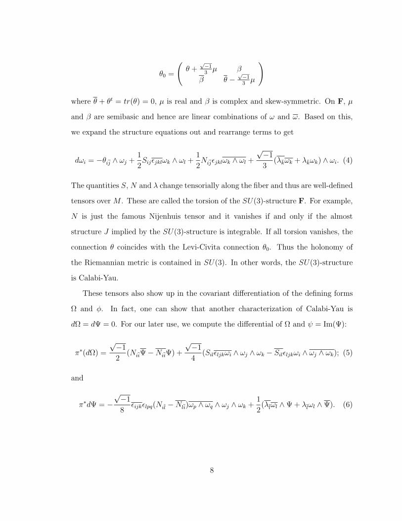
where θ + θt = tr(θ) = 0, µ is real and β is complex and skew-symmetric. On F, µ

and β are semibasic and hence are linear combinations of ω and ω. Based on this,

we expand the structure equations out and rearrange terms to get

dωi = −θij ∧ ωj +1

2Sijεjklωk ∧ ωl +

1

2Nijεjklωk ∧ ωl +

√−1

3(λkωk + λkωk) ∧ ωi. (4)

The quantities S, N and λ change tensorially along the fiber and thus are well-defined

tensors over M . These are called the torsion of the SU(3)-structure F. For example,

N is just the famous Nijenhuis tensor and it vanishes if and only if the almost

structure J implied by the SU(3)-structure is integrable. If all torsion vanishes, the

connection θ coincides with the Levi-Civita connection θ0. Thus the holonomy of

the Riemannian metric is contained in SU(3). In other words, the SU(3)-structure

is Calabi-Yau.

These tensors also show up in the covariant differentiation of the defining forms

Ω and φ. In fact, one can show that another characterization of Calabi-Yau is

dΩ = dΨ = 0. For our later use, we compute the differential of Ω and ψ = Im(Ψ):

π∗(dΩ) =

√−1

2(NiiΨ−NiiΨ) +

√−1

4(Silεljkωi ∧ ωj ∧ ωk − Silεljkωi ∧ ωj ∧ ωk); (5)

and

π∗dΨ = −√−1

8εijkεlpq(Nil −Nli)ωp ∧ ωq ∧ ωj ∧ ωk +

1

2(λlωl ∧Ψ + λlωl ∧Ψ). (6)

8

1

Special Lagrangian and SU(3)-Structures

1.1 Special Lagrangian geometry and admissible SU(3) structures

A submanifold L3 ⊂ M is called special Lagrangian if it is φ = ReΨ calibrated, i.e.,

if L∗(φ) is the volume form. The form φ is a calibration if it is closed. In this case

L is minimal. Assume L is orientable. Then L is special Lagrangian with one of its

orientations if and only if Ω|L = ψ|L = 0 where ψ = ImΨ. In other words it is an

integral manifold of the differential ideal I generated algebraically by Ω and ψ.

A generic SU(3)-structure will not admit any special Lagrangian submanifolds

at all, even locally. For example, if

dΩ ≡ aφ mod (Ω, ψ)

for some non-vanishing function a, then any special Lagrangian submanifold has to

annihilate dΩ and hence φ. Thus no special Lagrangian submanifold exists. We are

interested to know which SU(3)-structures support as many local special Lagrangian

submanifolds as the flat C3 does. If the SU(3)-structure is real analytic, so is the

ideal I. Now if dΩ ∈ I, then we may invoke the Cartan-Kahler theorem to show

9

that I is involutive and has the same Cartan characters as the ideal in C3. Here we

need not care about whether or not d(ImΨ) is in I because d(ImΨ) is of degree 3 + 1

and hence vanishes automatically on any 3-dimensional submanifold.

1.1.1 Admissible SU(3)-structures

We make the following definition.

Definition 1.1.1. (Admissible SU(3)-structures) An SU(3)-structure (Ω,Ψ) on M

is called admissible if there exist a 1-form θ and a real function a such that

dΩ = θ ∧ Ω + aψ. (1.1)

Suppose condition (1.1) is satisfied with

θ = uiωi + uiωi.

Then it also holds that

dΩ =

√−1

4(uiδjk − ujδik)ωi ∧ ωj ∧ ωk −

√−1

4(uiδkj − ujδki)ωi ∧ ωj ∧ ωk + aψ.

Comparing with (5), we get

εljkSil = ujδik − ukδij

and a = Nii. We summarize the discussion so far as follows:

Lemma 1.1.2. Suppose (M,Ω,Ψ) is analytic. The ideal I is involutive and every

Ω-Lagrangian analytic 2-submanifold in M6 can be thickened uniquely to a special

Lagrangian submanifold if there exists a (necessarily unique) connection α so that

dωi = −αij ∧ ωj + β ∧ ωi +1

2Nijεjklωk ∧ ωl (1.2)

where β is a complex 1-form and the trace of the Nijenhuis tensor, Nii, is real.

10

Remark 1.1.3. It is easy to see that the condition (1.2) in Lemma 1.1.2 essentially

gives an equivalent definition of admissible SU(3)-structures. For this reason, we

will also call an SU(3)-structure satisfying (1.2)admissible.

Remark 1.1.4. The same result for C3 was shown by Harvey and Lawson in [21].

Lemma 1.1.2 says an admissible SU(3)-manifold supports as nice a local special

Lagrangian geometry as C3 does. This is the best situation one can hope.

Out of these we pick a class of special interest and call it nearly Calabi-Yau.

Definition 1.1.5 (Nearly Calabi-Yau). An SU(3)-structure (M6,Ω,Ψ) is called

nearly Calabi-Yau if for some real function U ,

dΩ = d(eU ImΨ) = 0.

From (6), nearly Calabi-Yau condition amounts to Nij−Nji = 0 and√−1λl = Ul

where we have denoted π∗(dU) = Ulωl + Ulωl.

In terms of structure equations we have

Proposition 1.1.6. An SU(3)-structure is nearly Calabi-Yau for a real funciton U

if and only if there exists a (necessarily unique) connection α so that

dωi = −αij ∧ ωj +1

2Nijεjklωk ∧ ωl +

1

3(Ukωk − Ukωk) ∧ ωi, (1.3)

where dU = Ukωk + Ukωk, Nij −Nji = 0 and tr(N) = Nii = 0.

In other words, the Nijenhuis tensor is Hermitian symmetric and trace free.

Remark 1.1.7. This definition is motivated by two reasons. First, as we will see

shortly, it generalizes the concept of almost Calabi-Yau in that the underlying al-

most complex structure may not be integrable. Second, the moduli space of special

Lagrangian submanifolds of a nearly Calabi-Yau manifold is well-behaved. We will

prove this in §1.4.

11

Remark 1.1.8 (The case U = 0). When the defining function vanishes identically,

a nearly Calabi-Yau structure is also half-flat. A half-flat SU(3)-structure is defined

so that Ω ∧ dΩ = dImΨ = 0. This is in general not admissible. However, it has

been used by string physicists to study heterotic string compactifications for a long

time. In this context, half-flat manifolds are as important as Calabi-Yau structures.

Mathematically, it has been studied by S. Chiossi and S. Salamon in its relation with

G2-structures. They showed that this structure behaves well under Hitchin’s flow

equation [22]. Half-flat structures were also studied in [28].

In spite of much interest, few non-Calabi-Yau examples are known. In the next

subsection, we will analyze the local existence of half-flat nearly Calabi-Yau. We

will see that local half-flat nearly Calabi-Yau structures are much more general than

Calabi-Yau. In §1.2 we will construct a class of complete or even compact half-flat

nearly Calabi-Yau but non-Calabi-Yau examples.

1.1.2 First examples

Calabi-Yau

Calabi-Yau is clearly nearly Calabi-Yau. It is the case of most interest so far.

Almost Calabi-Yau

A more general SU(3)-structure is called almost Calabi-Yau in [23]. It is also con-

sidered by R. Bryant [10] and E. Goldstein [17]. An almost Calabi-Yau manifold is

a Kahler manifold with a nowhere vanishing holomorphic 3-form Φ specified. Let B

be the unique function such that

1

8

√−1Ψ ∧Ψ =

1

6B2Ω3.

It is clear that (Ω, ΦB, B) defines a nearly Calabi-Yau structure on M . Thus, an

almost Calabi-Yau structures is nearly Calabi-Yau.

12

Many interesting almost Calabi-Yau examples are provided by degree 5 smooth

varieties in CP 4. It is well-known that the canonical line bundle of such a variety is

trivial. Thus a nowhere vanishing holomorphic 3-form exists. However, the induced

Fubini-Study metric is not Calabi-Yau in general. These provide many almost Calabi-

Yau but non-Calabi-Yau examples.

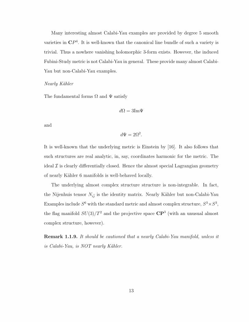
Nearly Kahler

The fundamental forms Ω and Ψ satisfy

dΩ = 3ImΨ

and

dΨ = 2Ω2.

It is well-known that the underlying metric is Einstein by [16]. It also follows that

such structures are real analytic, in, say, coordinates harmonic for the metric. The

ideal I is clearly differentially closed. Hence the almost special Lagrangian geometry

of nearly Kahler 6 manifolds is well-behaved locally.

The underlying almost complex structure structure is non-integrable. In fact,

the Nijenhuis tensor Nij is the identity matrix. Nearly Kahler but non-Calabi-Yau

Examples include S6 with the standard metric and almost complex structure, S3×S3,

the flag manifold SU(3)/T 2 and the projective space CP3 (with an unusual almost

complex structure, however).

Remark 1.1.9. It should be cautioned that a nearly Calabi-Yau manifold, unless it

is Calabi-Yau, is NOT nearly Kahler.

13

1.1.3 Generalities

Calabi-Yau and nearly Kahler provide first examples of admissible SU(3)-structures.

However, we are about to show that they are only a ‘closed’ subset of the moduli of

local admissible SU(3)-structures. For this, we need to study the local generality of

admissible SU(3)-structures.

Let p : F → M6 be the total coframe bundle of M6. Thus F is a principal

GL(6,R)-bundle over M6. The fiber Fx over x consists of the linear isomorphisms

u : TxM → R6. We consider the quotient F/SU(3) which is 34(= 6 + 62 − 8)

dimensional and projects onto M with fibers diffeomorphic to GL(6,R)/SU(3). An

SU(3)-structure over M may be regarded as a section of p : F/SU(3)→M6. In fact,

if P is an SU(3)-structure, then P is a subbundle of F and every fiber Px determines

a unique SU(3) orbit of Fx and thus a section of F/SU(3) → M6. Conversely, if

σ : M → F/SU(3) is such a section, let P be the preimage of σ(M) under the

projection F → F/SU(3). Then P is the needed SU(3)-structure.

Remark 1.1.10. There is a more concrete realization of F/SU(3). Let Λ2+M⊕Λ3

+M

be the subbundle of Λ2M ⊕ Λ3M consiting of the pairs of positive forms (ρ2, ρ3) in

the sense that there exists a linear isomorphism u : TxM → R6 such that ρ2 = u∗Ω0

and ρ3 = u∗Re(Ψ0). We clearly have a projection F → Λ2+M ⊕ Λ3

+M . Since the

isotropy group of (Ω0,ReΨ0) is SU(3) ⊂ GL(6,R), this is indeed a principal SU(3)-

bundle. For similar discussions concerning G2-structures and Spin(7)-structures,

consult Bryant’s work [7]. In fact, the work directly inspired the discussion in this

section.

We will write structures equations for F . For notational conventions on linear

algebra see Introduction. Let (ω1, ω2, ω3, ω1, ω2, ω3) denote complexified tautological

1-forms. Thus, for example, ω1u = u∗(dz1) p∗. We fix a gl(6,R)-valued connection

14

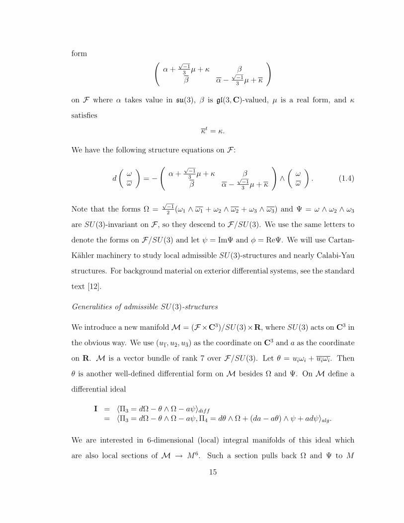
form (α +

√−13µ+ κ β

β α−√−13µ+ κ

)

on F where α takes value in su(3), β is gl(3,C)-valued, µ is a real form, and κ

satisfies

κt = κ.

We have the following structure equations on F :

d

(ωω

)= −

(α +

√−13µ+ κ β

β α−√−13µ+ κ

)∧(ωω

). (1.4)

Note that the forms Ω =√−12

(ω1 ∧ ω1 + ω2 ∧ ω2 + ω3 ∧ ω3) and Ψ = ω ∧ ω2 ∧ ω3

are SU(3)-invariant on F , so they descend to F/SU(3). We use the same letters to

denote the forms on F/SU(3) and let ψ = ImΨ and φ = ReΨ. We will use Cartan-

Kahler machinery to study local admissible SU(3)-structures and nearly Calabi-Yau

structures. For background material on exterior differential systems, see the standard

text [12].

Generalities of admissible SU(3)-structures

We introduce a new manifoldM = (F×C3)/SU(3)×R, where SU(3) acts on C3 in

the obvious way. We use (u1, u2, u3) as the coordinate on C3 and a as the coordinate

on R. M is a vector bundle of rank 7 over F/SU(3). Let θ = uiωi + uiωi. Then

θ is another well-defined differential form on M besides Ω and Ψ. On M define a

differential ideal

I = 〈Π3 = dΩ− θ ∧ Ω− aψ〉diff= 〈Π3 = dΩ− θ ∧ Ω− aψ,Π4 = dθ ∧ Ω + (da− aθ) ∧ ψ + adψ〉alg.

We are interested in 6-dimensional (local) integral manifolds of this ideal which

are also local sections of M → M6. Such a section pulls back Ω and Ψ to M

15

which satisfies the condition (1.1) and thus defines an admissible SU(3)-structure.

A section satisfies√−1Ψ ∧ Ψ 6= 0. Conversely a 6-dimensional submanifold of M

on which√−1Ψ ∧ Ψ 6= 0 is locally a section. Hence we will consider the integral

manifolds of I with the independence condition√−1Ψ ∧Ψ 6= 0.

Theorem 1.1.11. The differential system (I,√−1Ψ∧Ψ 6= 0) on the dense open set

M\ a = 0 is involutive with Cartan characters

(s0, s1, s2, s3, s4, s5, s6) = (0, 0, 1, 3, 6, 10, 15).

Proof. Since the system contains no forms of degree 2 or less, we have c0 = c1 = 0.

On the other hand, c1 = 1 and c6 = 35. We need to compute the remaining three

characters c3, c4 and c5. For this we pass up to F×C3×R. For effective computations

we set

Da = da− aθ,

and

Dui = dui − ujαji − ujκji −√−1

3uiµ− ujβji.

Relative to the projection F × C3 × R → M, the forms ω, κ, β, µ,Da,Du form a

basis for semibasic 1-forms. In terms of these forms we have

Π3 = −√−12κij ∧ ωj ∧ ωi +

√−12κij ∧ ωj ∧ ωi

−√−14

(βij − βji) ∧ ωj ∧ ωi +√−14

(βij − βji) ∧ ωj ∧ ωi

−√−12

(uiωi + uiωi) ∧ ωj ∧ ωj

−√−12a(ω1 ∧ ω2 ∧ ω3 − ω1 ∧ ω2 ∧ ω3)

16

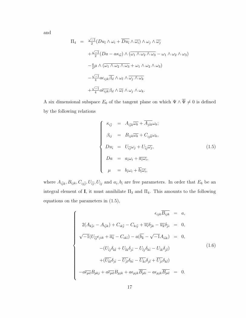
and

Π4 =√−12

(Dui ∧ ωi +Dui ∧ ωi) ∧ ωj ∧ ωj

+√−12

(Da− aκii) ∧ (ω1 ∧ ω2 ∧ ω3 − ω1 ∧ ω2 ∧ ω3)

−a2µ ∧ (ω1 ∧ ω2 ∧ ω3 + ω1 ∧ ω2 ∧ ω3)

−√−14aεijkβil ∧ ωl ∧ ωj ∧ ωk

+√−14aεijkβil ∧ ωl ∧ ωj ∧ ωk.

A six dimensional subspace E6 of the tangent plane on which Ψ ∧ Ψ 6= 0 is defined

by the following relations

κij = Aijkωk + Ajikωk;

βij = Bijkωk + Cijkωk,

Dui = Uijωj + Uijωj,

Da = aiωi + aiωi,

µ = biωi + biωi,

(1.5)

where Aijk, Bijk, Cijj, Uij, Uij and ai, bi are free parameters. In order that E6 be an

integral element of I, it must annihilate Π3 and Π4. This amounts to the following

equations on the parameters in (1.5),

εijkBijk = a,

2(Akji − Aijk) + Cikj − Ckij + uiδjk − ukδji = 0,

√−1(Uijεjik + ak − Ciki)− a(bk −

√−1Aiik) = 0,

−(Uijδkl + Ulkδji − Uljδki − Uikδjl)

+(Uklδji − Ujlδki − Ukiδjl + Ujiδkl)

−aεpilBpkj + aεpilBpjk + aεpjkBpli − aεpjkBpil = 0.

(1.6)

17

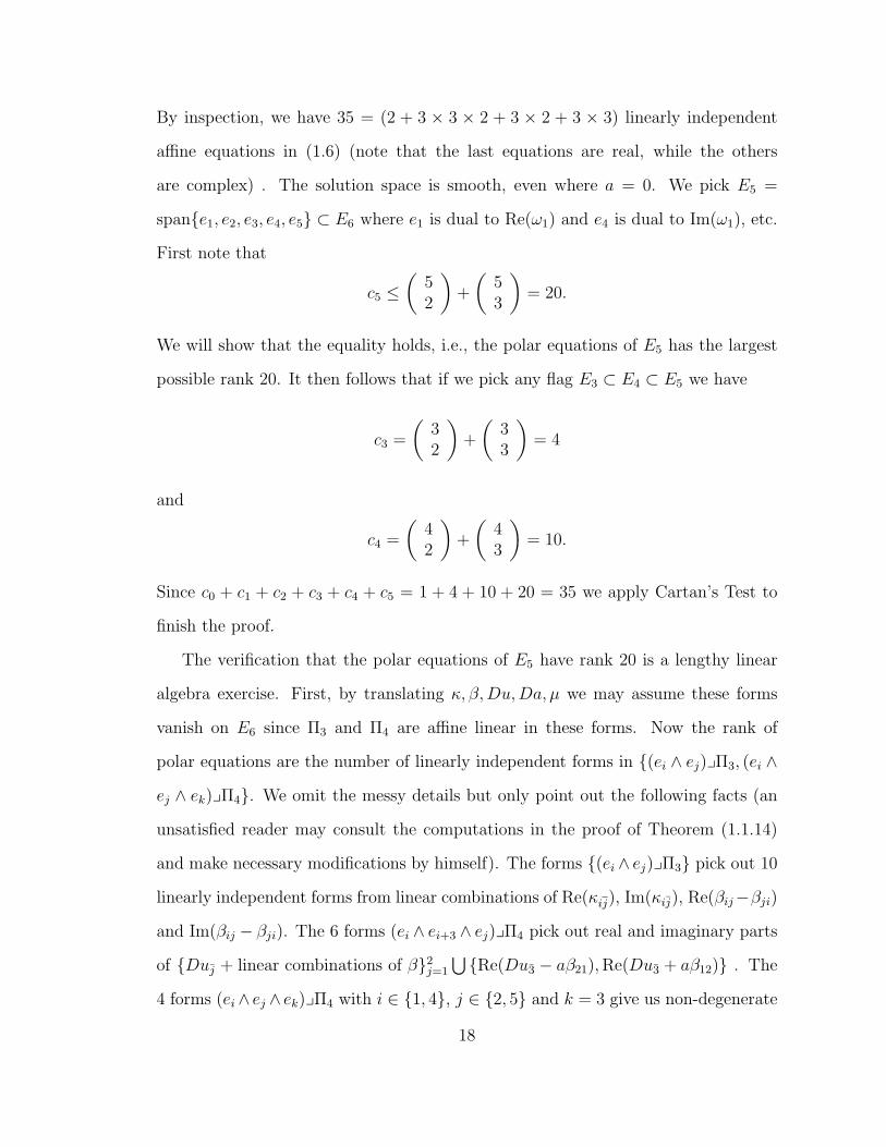
By inspection, we have 35 = (2 + 3 × 3 × 2 + 3 × 2 + 3 × 3) linearly independent

affine equations in (1.6) (note that the last equations are real, while the others

are complex) . The solution space is smooth, even where a = 0. We pick E5 =

spane1, e2, e3, e4, e5 ⊂ E6 where e1 is dual to Re(ω1) and e4 is dual to Im(ω1), etc.

First note that

c5 ≤(

52

)+

(53

)= 20.

We will show that the equality holds, i.e., the polar equations of E5 has the largest

possible rank 20. It then follows that if we pick any flag E3 ⊂ E4 ⊂ E5 we have

c3 =

(32

)+

(33

)= 4

and

c4 =

(42

)+

(43

)= 10.

Since c0 + c1 + c2 + c3 + c4 + c5 = 1 + 4 + 10 + 20 = 35 we apply Cartan’s Test to

finish the proof.

The verification that the polar equations of E5 have rank 20 is a lengthy linear

algebra exercise. First, by translating κ, β,Du,Da, µ we may assume these forms

vanish on E6 since Π3 and Π4 are affine linear in these forms. Now the rank of

polar equations are the number of linearly independent forms in (ei ∧ ej)yΠ3, (ei ∧

ej ∧ ek)yΠ4. We omit the messy details but only point out the following facts (an

unsatisfied reader may consult the computations in the proof of Theorem (1.1.14)

and make necessary modifications by himself). The forms (ei ∧ ej)yΠ3 pick out 10

linearly independent forms from linear combinations of Re(κij), Im(κij), Re(βij−βji)

and Im(βij − βji). The 6 forms (ei ∧ ei+3 ∧ ej)yΠ4 pick out real and imaginary parts

of Duj + linear combinations of β2j=1

⋃Re(Du3 − aβ21),Re(Du3 + aβ12) . The

4 forms (ei∧ ej ∧ ek)yΠ4 with i ∈ 1, 4, j ∈ 2, 5 and k = 3 give us non-degenerate

18

linear combinations of the forms Da−a∑κii, aµ, aRe(βii) and aIm(βii). These three

classes of equations are clearly independent from each other if we assume a 6= 0.

Remark 1.1.12. There does not exist any regular flag over the locus a = 0 for

simple reasons. When a = 0, only 7 independent forms Dui and Da in Π4 could

contribute to the polar equations. Thus c5 ≤ 17.

Remark 1.1.13. The last nonzero character is s6 = 15. Modulo diffeomorphisms,

which depend on 6 functions of 6 variables, we still have 9 functions of 6 variables

of local generality of admissible SU(3)-structures. Both local Calabi-Yau and nearly

Kahler structures depend on 2 functions of 5 variables. Thus local admissible SU(3)-

structures are much more general than Calabi-Yau and nearly Kahler.

Generality of nearly Calabi-Yau

Nearly Calabi-Yau is a subclass of admissible SU(3)-structures. One would expect

nearly Calabi-Yau to be less general than an admissible SU(3)-structure. We will

show this is indeed the case. Now the differential system I is defined on F/SU(3)×R

and generated algebraically by the 3-form dΩ and the 4-form Υ = dψ+ dU ∧ψ with

the independence condition√−1Ψ ∧ Ψ. This system is better-behaved than I for

admissible SU(3)-structures in that it is involutive on the whole F/SU(3)×R.

Theorem 1.1.14. The differential system I on F/SU(3) × R is involutive with

Cartan characters (s0, s1, s2, s3, s4, s5, s6) = (0, 0, 1, 3, 6, 9, 10).

Proof. Since the system contains no forms of degree 2 or less, we have c0 = c1 = 0.

Moreover, it is easy to see c2 = 1. To use Cartan’s Test, we need compute the other

3 characters c3, c4 and c5 and the codimension of the space of 6-dimensional integral

elements. For this we pass up to F where

dΩ = −√−12κijωj ∧ ωi +

√−12κijωj ∧ ωi

−√−12βij ∧ ωj ∧ ωi +

√−12βij ∧ ωj ∧ ωi,

19

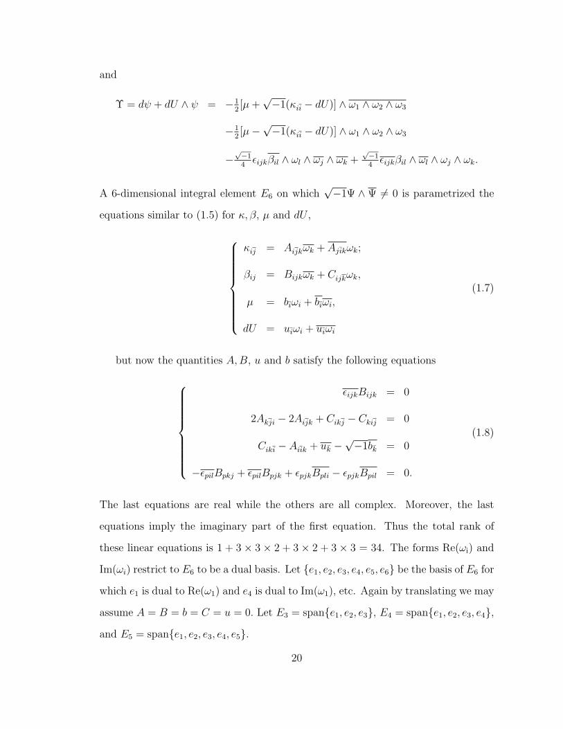
and

Υ = dψ + dU ∧ ψ = −12[µ+

√−1(κii − dU)] ∧ ω1 ∧ ω2 ∧ ω3

−12[µ−

√−1(κii − dU)] ∧ ω1 ∧ ω2 ∧ ω3

−√−14εijkβil ∧ ωl ∧ ωj ∧ ωk +

√−14εijkβil ∧ ωl ∧ ωj ∧ ωk.

A 6-dimensional integral element E6 on which√−1Ψ ∧ Ψ 6= 0 is parametrized the

equations similar to (1.5) for κ, β, µ and dU ,

κij = Aijkωk + Ajikωk;

βij = Bijkωk + Cijkωk,

µ = biωi + biωi,

dU = uiωi + uiωi

(1.7)

but now the quantities A,B, u and b satisfy the following equations

εijkBijk = 0

2Akji − 2Aijk + Cikj − Ckij = 0

Ciki − Aiik + uk −√−1bk = 0

−εpilBpkj + εpilBpjk + εpjkBpli − εpjkBpil = 0.

(1.8)

The last equations are real while the others are all complex. Moreover, the last

equations imply the imaginary part of the first equation. Thus the total rank of

these linear equations is 1 + 3 × 3 × 2 + 3 × 2 + 3 × 3 = 34. The forms Re(ωi) and

Im(ωi) restrict to E6 to be a dual basis. Let e1, e2, e3, e4, e5, e6 be the basis of E6 for

which e1 is dual to Re(ω1) and e4 is dual to Im(ω1), etc. Again by translating we may

assume A = B = b = C = u = 0. Let E3 = spane1, e2, e3, E4 = spane1, e2, e3, e4,

and E5 = spane1, e2, e3, e4, e5.

20

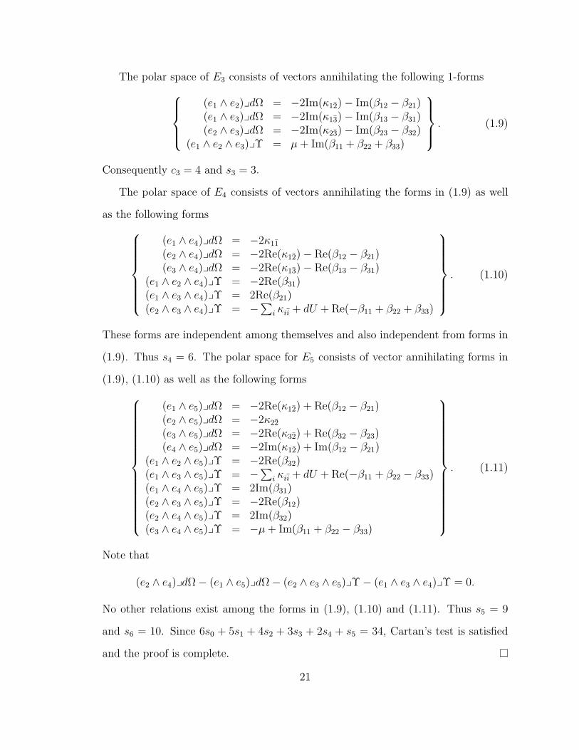
The polar space of E3 consists of vectors annihilating the following 1-forms(e1 ∧ e2)ydΩ = −2Im(κ12)− Im(β12 − β21)(e1 ∧ e3)ydΩ = −2Im(κ13)− Im(β13 − β31)(e2 ∧ e3)ydΩ = −2Im(κ23)− Im(β23 − β32)

(e1 ∧ e2 ∧ e3)yΥ = µ+ Im(β11 + β22 + β33)

. (1.9)

Consequently c3 = 4 and s3 = 3.

The polar space of E4 consists of vectors annihilating the forms in (1.9) as well

as the following forms

(e1 ∧ e4)ydΩ = −2κ11

(e2 ∧ e4)ydΩ = −2Re(κ12)− Re(β12 − β21)(e3 ∧ e4)ydΩ = −2Re(κ13)− Re(β13 − β31)

(e1 ∧ e2 ∧ e4)yΥ = −2Re(β31)(e1 ∧ e3 ∧ e4)yΥ = 2Re(β21)(e2 ∧ e3 ∧ e4)yΥ = −

∑i κii + dU + Re(−β11 + β22 + β33)

. (1.10)

These forms are independent among themselves and also independent from forms in

(1.9). Thus s4 = 6. The polar space for E5 consists of vector annihilating forms in

(1.9), (1.10) as well as the following forms

(e1 ∧ e5)ydΩ = −2Re(κ12) + Re(β12 − β21)(e2 ∧ e5)ydΩ = −2κ22

(e3 ∧ e5)ydΩ = −2Re(κ32) + Re(β32 − β23)(e4 ∧ e5)ydΩ = −2Im(κ12) + Im(β12 − β21)

(e1 ∧ e2 ∧ e5)yΥ = −2Re(β32)(e1 ∧ e3 ∧ e5)yΥ = −

∑i κii + dU + Re(−β11 + β22 − β33)

(e1 ∧ e4 ∧ e5)yΥ = 2Im(β31)(e2 ∧ e3 ∧ e5)yΥ = −2Re(β12)(e2 ∧ e4 ∧ e5)yΥ = 2Im(β32)(e3 ∧ e4 ∧ e5)yΥ = −µ+ Im(β11 + β22 − β33)

. (1.11)

Note that

(e2 ∧ e4)ydΩ− (e1 ∧ e5)ydΩ− (e2 ∧ e3 ∧ e5)yΥ− (e1 ∧ e3 ∧ e4)yΥ = 0.

No other relations exist among the forms in (1.9), (1.10) and (1.11). Thus s5 = 9

and s6 = 10. Since 6s0 + 5s1 + 4s2 + 3s3 + 2s4 + s5 = 34, Cartan’s test is satisfied

and the proof is complete.

21

Thus, modulo diffeomorphisms, local nearly Calabi-Yau structures depend on 4

functions of 6 variables.

Remark 1.1.15 (Generality of half-flat nearly Calabi-Yau structures). The EDS

for half-flat nearly Calabi-Yau structures is defined on F/SU(3) and algebraically

generated by dΩ and dImΨ. Similar analysis shows that this system is also involutive

with Cartan characters

(s0, s1, s2, s3, s4, s5, s6) = (0, 0, 1, 3, 6, 9, 9).

Thus, modulo diffeomorphisms, these structures depend on 3 functions of 6 vari-

ables locally. They are much more general than Calabi-Yau structures. It would be

interesting to also analyze the half flat system generated by Ω ∧ dΩ and dImΨ.

Remark 1.1.16 (Generality of almost Calabi-Yau structues). The EDS for almost

Calabi-Yau structures is defined on F/SU(3)×R and generated algebraically by dΩ

and dΨ + dU ∧ Ψ. We conjecture this system is involutive with the last non-zero

Cartan character to be s6 = 7. We leave this for the interested reader to investigate.

1.2 Examples from twistor spaces of Riemannian four-manifolds

There has been an extensive literature on twistor theory. Suppose (M4, ds2) is a

Riemannian 4-manifold. A twistor at x ∈ M is an orthogonal complex structure

j : TxM → TxM , j2 = −1 and j∗(ds2x) = ds2

x. The space of twistors at points of M

forms a smooth manifold J called twistor space of M . It is well-known that J has

an almost complex structure. It is moreover complex if M has constant sectional

curvatures. However, we will not use this usual almost complex structure in this

paper. Instead, we will ‘reverse’ the almost complex structure on the fibers and

obtain an SU(3)-structure on J . By doing so, we will lose the possible integrability

of the almost complex structures in some cases.

22

1.2.1 Four dimensional Riemannian geometry

We formulate Riemannian geometry of four-manifolds in moving frames. Let π :

F → M be the oriented orthonormal coframe bundle over M . Thus Fx consists of

orientation preserving isometries u : TxM → R4. Let η be the R4-valued tautological

form on F . By the fundamental theorem of Riemannian geometry, there exists a

unique so(4,R)-valued one-form θ so that

dη = −θ ∧ η.

Denote ω1 = η1 +√−1η3 and ω2 = η2 +

√−1η4. We write the structrure equation as

d

ω1

ω2

ω1

ω2

= −(αij βijβij αij

)∧

ω1

ω2

ω1

ω2

(1.12)

where αt + α = 0 and βt + β = 0. The Riemannian curvature is of course

R = d

(α ββ α

)+

(α ββ α

)∧(α ββ α

).

This is a so(4,R)-valued 2-form. Corresponding to the decomposition so(4,R) =

su(2)+ ⊕ su(2)− we decompose R = R+ +R−, where

R+ = d

(α0 00 α0

)+

(α0 00 α0

)∧(α0 00 α0

)and

R− = d

(12tr(α)I β

β 12tr(α)I

)+

(12tr(α)I β

β 12tr(α)I

)∧(

12tr(α)I β

β 12tr(α)I

).

for which α0 = α− 12tr(α)I takes value in su(2). We are mainly interested in R− so

we examine this part more carefully. Write

β =

(0 ω3

−ω3 0

),

23

(R−)1 =1

2dtr(α) + ω3 ∧ ω3,

and

(R−)2 = dω3 − tr(α) ∧ ω3.

The forms

Θ1 = ω1 ∧ ω2, Θ2 = ω1 ∧ ω2, Θ3 =

√−1

2(ω1 ∧ ω1 + ω2 ∧ ω2)

give a basis for anti-self dual complex forms at x, while

Σ1 = ω1 ∧ ω2, Σ2 = ω1 ∧ ω2, Σ3 =

√−1

2(ω1 ∧ ω1 − ω2 ∧ ω2)

form a basis for self dual forms at x. Since R− is semibasic,

(R−)1 = AΘ1 − AΘ2 +√−1aΘ3 +BΣ1 −BΣ2 +

√−1bΣ3,

and

(R−)2 = C1Θ1 + C2Θ2 + C3Θ3 +D1Σ1 +D2Σ2 +D3Σ3

where A,B,Ci, Di are complex and a, b are real. For our purposes, we view R− as a

(2, 2) tensor. Using ds2, we write R as

R− = 2(R−)1 ⊗ (E1 ∧ E1 + E2 ∧ E2) + 2(R−)2 ⊗ E1 ∧ E2 + 2(R−)2 ⊗ E1 ∧ E2

= 2√−1(R−)1 ⊗Θ∗3 + 2(R−)2 ⊗Θ∗2 + 2(R−)2 ⊗Θ∗1

where, by abuse of notation, we use Ei to denote the tangent vector dual to ωi. In

this way we may regard R− as a linear map R− : Λ2− → Λ2 = Λ2

− ⊕ Λ2+. Relative to

the basis Θ and Σ we write the matrix representation

R−(Θ1,Θ2,Θ3) = 2(Θ1,Θ2,Θ3,Σ1,Σ2,Σ3)

C2 C1

√−1A

C1 C2 −√−1A

C3 C3 −aD2 D1

√−1B

D1 D2 −√−1B

D3 D3 −b

.

24

It is well-known that R− decomposes as Z + W− + s12Id (see [6], p. 51) where Z

is the traceless Ricci curvature, W− is the anti-self-dual part of the Weyl curvature

and s is the scalar curvature. In our notation, Z is represented by the matrix

2

D2 D1

√−1B

D1 D2 −√−1B

D3 D3 −b

,

s = 8(C2 + C2 − a),

and W− is represented by

2

C2 C1

√−1A

C1 C2 −√−1A

C3 C3 −a

− 2

3(C2 + C2 − a)I.

The metric with W− = 0 is called self-dual. If in addition, ds2 is Einstein, then

s is necessarily constant. In our notations,

Proposition 1.2.1. The metric ds2 is self-dual and Einstein if and only if b = A =

B = C1 = C3 = D1 = D2 = D3 = 0 and C2 = C2 = −a = s24

. In this case, a part of

the structure equation simplifies greatly

d

ω1

ω2

ω3

= −(α 00 −tr(α)

)∧

ω1

ω2

ω3

+

ω2 ∧ ω3

ω3 ∧ ω1s24ω1 ∧ ω2

. (1.13)

Self-dual Einstein metrics will play important roles in our following constructions.

There are not many compact examples with s ≥ 0 due to the classification by Hitchin

(see [6], p 376):

Theorem 1.2.2. Let M be be self-dual Einstein manifold. Then

(1) If s > 0, M is isometric to S4 or CP 2 with their canonical metrics.

(2) If s = 0, M is either flat or its universal covering is a K3 surface with the

Calabi-Yau metric.

25

The proof uses Bochner Technique, which, however does not work well when

s < 0. No similar results are available for self-dual Einstein metrics with negative

scalar curvature.

1.2.2 Twistor spaces of self-dual Einstein 4-manifolds

We fix a complex structure J0 on R4 by requiring dz1 = dx1 +√−1dx3 and dz2 =

dx2 +√−1dx4 be complex linear. We define a map j : F → J as follows

j(u) = u−1 J0 u.

Since SO(4) acts transitively on the orthogonal complex structures on R4 and the

isotropy group of J0 is U(2), j makes F a principal U(2)-bundle over J . This

defines a U(2)-structure on J . It in turn determines an SU(3)-structure on J by

the standard embedding of U(2) into SU(3). Relative to j, β becomes semi-basic.

The almost structure on J determined by this SU(3)-strucure is such that ω1, ω2

and ω3 are complex linear.

Let us now concentrate on self-dual Einstein manifolds. The equations in (1.13)

are the first structure equations on J . It clearly satisfies the condition of Lemma

1.1.2.

Lemma 1.2.3. The twistor space of a self-dual Einstein 4-manifold carries an ad-

missible SU(3)-structure.

s > 0

In this case, we scale the metric so that s = 24. Now the structure equation (1.13)

indicates that the twistor space is actually nearly Kahler. By the aforementioned

Hitchin’s result, the only two possibilities are M = S4 and M = CP2. The corre-

sponding twistor spaces are two familiar nearly Kahler examples, CP3 and the flag

manifold SU(3)/T 2.

26

s = 0

Again, by Hitchin’s result we have two examples: one is the flat case, the other is

K3 surfaces.

s < 0

This is the most interesting case in many respects. We scale the metric to make

s = −48. Now the structure equation (1.13) reads

d

ω1

ω2

ω3

= −(α 00 −tr(α)

)∧

ω1

ω2

ω3

+

ω2 ∧ ω3

ω3 ∧ ω1

−2ω1 ∧ ω2

. (1.14)

The only torsion is the Nijenhuis tensor, in local unitary basis,

N =

1 0 00 1 00 0 −2

.

Comparing with (1.3) (with U = 0 being understood), we have

Theorem 1.2.4. The twistor space of a self-dual Einstein manifold of negative scalar

curvature is half-flat nearly Calabi-Yau but non-Calabi-Yau.

The simplest example of this category is, of course, the twistor space of the

hyperbolic space H4. Compact examples can be obtained from the quotients of

H4 by certain discrete isometry groups. It remains open to construct complete or

compact nearly Calabi-Yau manifolds that are not half-flat.

1.3 Complete special Lagrangian examples

In this section we will construct some complete special Lagrangian submanifolds in

the twistor spaces J (S4) = CP3 and J (H4) considered in the previous section. Our

27

method is based on the following observation due to Robert Bryant [8]. Suppose on

an SU(3) manifold (M,Ω,Ψ), there is a real structure, i.e., an involution c such that

c∗Ω = −Ω, c∗Ψ = Ψ,

and the set Nc of points fixed under c is a smooth submanifold. Then it is easy to see

that Nc, with one of its two possible orientations, is a special Lagrangian submanifold

of M . Thus our major task is to construct such involutions for J (S4) = CP3 and

J (H4).

1.3.1 An example in J (S4) = CP3

We need a more explicit description of the twistor fibration T : CP3 → S4. We

follow the discussion in [9]. However, as aforementioned, we will use a different

almost complex structure on CP3.

Let H denote the real division algebra of quaternions. An element of H can be

written uniquely as q = z + jw where z, w ∈ C and j ∈ H satisfies

j2 = −1, zj = jz

for all z ∈ C. The quaternion multiplication is thus given by

(z1 + jz2)(z3 + jz4) = z1z3 − z2z4 + j(z2z3 + z1z4). (1.15)

We define an involution C : H → H by C(z1 + jz2) = z1 + jz2. It can be easily

checked via the product rule (1.15) that this is in fact an algebra automorphism, i.e.,

C(pq) = C(p)C(q) for p, q ∈ H.

We regard C as subalgebra of H and give H the structure of a complex vector

space by letting C act on the right. We let H2 denote the space of pairs (q1, q2)

where qi ∈ H. We will make H2 into a quaternion vector space by letting H act on

the right

(q1, q2)q = (q1q, q2q).

28

This automatically makes H2 into a complex vector space of dimension 4. In fact,

regarding C4 as the space of 4-tuples (z1, z2, z3, z4), we make the explicit identification

(z1, z2, z3, z4) ∼ (z1 + jz2, z3 + jz4). (1.16)

This specific isomorphism is the one we will always mean when we write C4 = H2.

If v ∈ H2\(0, 0) is given, let vC and vH denote, respectively, the complex line and

the quaternion line spanned by v. As is well-known, HP1, the space of quaternion

lines in H2, is isometric to S4. For this reason, we will speak interchangeably of S4 and

HP1. The assignment vC → vH is exactly the twistor mapping T : CP3 → HP1.

The fibres of T are CP1’s. Thus, we have a fibration

CP1 → CP3

↓HP1

(1.17)

This is the famous twistor fibration. In order to study its geometry more thoroughly,

we will now introduce the structure equations of H2. First we endow H2 with a

quaternion inner product 〈, 〉 : H2 ×H2 → H defined by

〈(q1, q2), (p1, p2)〉 = q1p1 + q2p2.

We have identities

〈v, wq〉 = 〈v, w〉 q, 〈v, w〉 = 〈w, v〉 , 〈vq, w〉 = q 〈v, w〉 .

Via the identification (1.16),

〈(q1, q2), (p1, p2)〉 = z1w1 + z2w2 + z3w3 + z4w4

+j(z1w2 − z2w1 + z3w4 − z4w3)(1.18)

for q1 = z1 + jz2, q2 = z3 + jz4, p1 = w1 + jw2, p2 = w3 + jw4. In other words,

〈, 〉 essentially consists of two parts: one is the standard Hermitian product dz1dz1+

· · ·+dz4dz4; the other is the standard complex symplectic form dz1∧dz2 +dz3∧dz4.

29

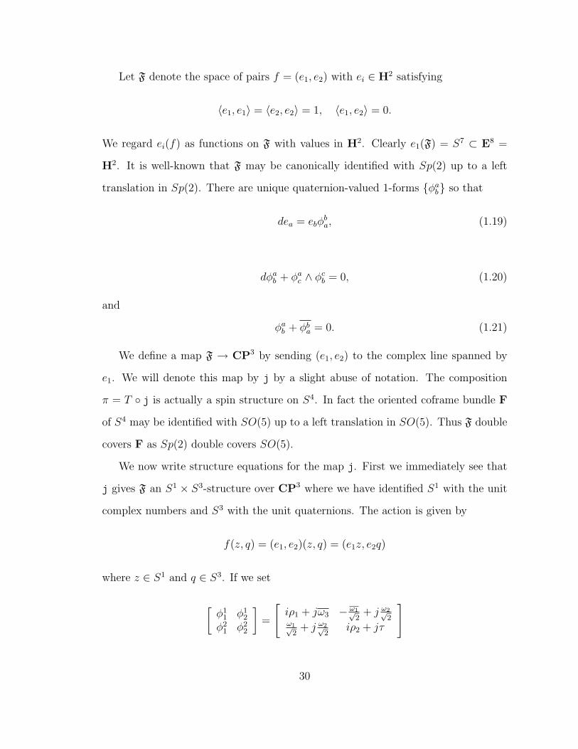
Let F denote the space of pairs f = (e1, e2) with ei ∈ H2 satisfying

〈e1, e1〉 = 〈e2, e2〉 = 1, 〈e1, e2〉 = 0.

We regard ei(f) as functions on F with values in H2. Clearly e1(F) = S7 ⊂ E8 =

H2. It is well-known that F may be canonically identified with Sp(2) up to a left

translation in Sp(2). There are unique quaternion-valued 1-forms φab so that

dea = ebφba, (1.19)

dφab + φac ∧ φcb = 0, (1.20)

and

φab + φba = 0. (1.21)

We define a map F → CP3 by sending (e1, e2) to the complex line spanned by

e1. We will denote this map by j by a slight abuse of notation. The composition

π = T j is actually a spin structure on S4. In fact the oriented coframe bundle F

of S4 may be identified with SO(5) up to a left translation in SO(5). Thus F double

covers F as Sp(2) double covers SO(5).

We now write structure equations for the map j. First we immediately see that

j gives F an S1 × S3-structure over CP3 where we have identified S1 with the unit

complex numbers and S3 with the unit quaternions. The action is given by

f(z, q) = (e1, e2)(z, q) = (e1z, e2q)

where z ∈ S1 and q ∈ S3. If we set

[φ1

1 φ12

φ21 φ2

2

]=

[iρ1 + jω3 − ω1√

2+ j ω2√

2ω1√

2+ j ω2√

2iρ2 + jτ

]

30

where ρ1 and ρ2 are real 1-forms while ω1, ω2, ω3 and τ are complex valued, we may

rewrite one part of the structure equation (3.3) relative to the S1 × S3-structure on

CP3 as

d

ω1

ω2

ω3

= −

i(ρ2 − ρ1) −τ 0τ −i(ρ1 + ρ2) 00 0 2iρ1

∧ ω1

ω2

ω3

+

ω2 ∧ ω3

ω3 ∧ ω1

ω1 ∧ ω2

.

(1.22)

The nearly Kahler structure on CP3 is defined by setting ω1, ω2 and ω3 to be complex

linear.

Via the algebra automorphism C we define an involution on H2 by (p, q) 7→

(C(p), C(q)). We denote this map still by C. This map in turn induces an involution

on F, still denoted C, by C(e1, e2) = (C(e1), C(e2)). From (1.18) we see that the

defining equations for F are preserved and the involution is well-defined. The map

C further descends to an involution c on CP3 as well as an involution c on S4 by

e1C 7→ C(e1)C and e1H 7→ C(e1)H respectively. We have the following commutative

diagram

FC−→ F

↓ ↓CP3 c−→ CP3

↓ ↓HP1 c−→ HP1

.

Apply the automorphism to the structure equations (3.2) and we get

dC(ea) = C(eb)C(φba).

Thus in particular we have on F

C∗ωi = ωi

for i = 1, 2, 3. Consequently

C∗j∗Ω = −j∗Ω, C∗j∗Ψ = j∗Ψ.

31

Since jC = cj and j∗ is injective, we have on CP3

c∗Ω = −Ω, c∗Ψ = Ψ.

Thus by the general principle the fixed set of c is a special Lagrangian submanifold

of CP3. Moreover it is easy to see that this locus is just the usual RP3.

Theorem 1.3.1. The real projective space RP3 = [x1 : x2 : x3 : x4] : xi ∈ R ⊂

CP3 is a special Lagrangian submanifold of the nearly Kahler CP3.

The twistor map T : CP3 → HP1 restricted to the real projective space RP3

now looks like

[x1 : x2 : x3 : x4] 7→ [x1 + jx2 : x3 + jx4].

Thus the image is a CP1 ⊂ HP1 and T is the Hopf fibration

S1 → RP3

↓CP1

.

A dual construction for J (H4) will follow.

1.3.2 An example in J (H4)

Let H2 and the involution C be as before. But now we endow H2 with a (1, 1)

quaternion inner product 〈, 〉 : H2 ×H2 → H defined by

〈(q1, q2), (p1, p2)〉 = q1p1 − q2p2.

We still have the identities

〈v, wq〉 = 〈v, w〉 q, 〈v, w〉 = 〈w, v〉 , 〈vq, w〉 = q 〈v, w〉 .

Via the identification (1.16),

〈(q1, q2), (p1, p2)〉 = z1w1 + z2w2 − z3w3 − z4w4

+j(z1w2 + z2w1 − z3w4 − z4w3)(1.23)

32

for q1 = z1+jz2, q2 = z3+jz4, p1 = w1+jw2, p2 = w3+jw4. In other words, 〈, 〉

essentially consists of two parts: one is the (2, 2)-Hermitian product dz1 dz1 + dz2

dz2−dz3dz3−dz4dz4; the other is a complex symplectic form dz1∧dz2−dz3∧dz4.

Denote the pseudo-sphere in H2 by

ΨS7 = (p, q) ∈ H2 : pp− qq = 1.

This is a connected non-compact smooth hypersurface in H2. The group S3 acts on

ΨS7 by

(p, q) · r = (pr, qr)

where r ∈ S3 is a unit quaternion number. This action is clearly free. Thus the

quotient space ΨHP1 = ΨS7/S3 is smooth. Indeed ΨHP1 = H4. Similarly if we

regard S1 as a subgroup of S3 consisting of unit complex numbers, the quotient

space ΨCP3 = ΨS7/S1 is smooth. The clearly well-defined map T : ΨCP3 → H4 is

exactly the twistor fibration of H4. We have the following commutative diagram of

fibrations

S1 → ΨS7

↓CP1 → ΨCP3

↓ΨHP1

.

Let F denote the space of pairs f = (e1, e2) with ei ∈ H2 satisfying

〈e1, e1〉 = 1, 〈e2, e2〉 = −1, 〈e1, e2〉 = 0.

We regard ei(f) as functions on F with values in H2. Clearly e1(F) = ΨS7 ⊂E(4,4) =

H2. It is well-known that F maybe canonically identified with Sp(1, 1) up to a left

translation in Sp(1, 1), where

Sp(1, 1) = A ∈ gl(2,H) : A

(1 00 −1

)At =

(1 00 −1

).

33

There are unique quaternion-valued 1-forms φab so that

dea = ebφba, (1.24)

dφab + φac ∧ φcb = 0, (1.25)

and

φ

(1 00 −1

)+

(1 00 −1

)φt = 0. (1.26)

We have a canonical map F→ ΨCP3 by sending (e1, e2) to the coset e1 · S1. We

will denote this map by j by a slight abuse of notation. The composition π = T j

is actually a spin structure on H4. In fact, the oriented coframe bundle F of H4

may be identified with SO0(4, 1), the identity component of SO(4, 1), up to a left

translation in SO0(4, 1). Thus F double covers F as Sp(1, 1) double covers SO0(4, 1)

(see Harvey [20], p. 272 for the isomorphism Sp(1, 1) ∼= Spin0(4, 1) where he used

the notation HU(1, 1) for Sp(1, 1)).

We now write structure equations for the map j. First we immediately see that

j gives F an S1×S3-structure over ΨCP3 where we have identified S1 with the unit

complex numbers and S3 with the unit quaternions. The action is given by

f(z, q) = (e1, e2) · (z, q) = (e1z, e2q)

where z ∈ S1 and q ∈ S3. If we set

[φ1

1 φ12

φ21 φ2

2

]=

[iρ1 + jω3 ω1 − jω2

ω1 + jω2 iρ2 + jτ

]

where ρ1 and ρ2 are real 1-forms while ω1, ω2, ω3 and τ are complex valued, we may

rewrite one part of the structure equation (3.3) relative to the nearly Calabi-Yau

34

structure on ΨCP3 as

d

ω1

ω2

ω3

= −

i(ρ2 − ρ1) −τ 0τ −i(ρ1 + ρ2) 00 0 2iρ1

∧ ω1

ω2

ω3

+

ω2 ∧ ω3

ω3 ∧ ω1

−2ω1 ∧ ω2

.

(1.27)

The nearly Calabi-Yau structure on ΨCP3 is defined by taking ω1, ω2 and ω3 to be

complex linear.

This involution C on H2 induces an involution on F, still denoted by C, by

C(e1, e2) = (C(e1), C(e2)). From (1.23), we see that the defining equations for F

are preserved and the involution is well-defined. The map C further descends to an

involution c on ΨCP3 as well as an involution c on H4 by e1 · S1 7→ C(e1) · S1 and

e1 · S3 7→ C(e1) · S3 repectively. We have the following commutative diagram

FC−→ F

↓ ↓ΨCP3 c−→ ΨCP3

↓ ↓H4 c−→ H4

.

Apply the automorphism to the structure equations (1.24) and we get

dC(ea) = C(eb)C(φba).

Thus in particular we have on F

C∗ωi = ωi

for i = 1, 2, 3. Consequently

C∗j∗Ω = −j∗Ω, C∗j∗Ψ = j∗Ψ.

Since jC = cj and j∗ is injective, we have on ΨCP3

c∗Ω = −Ω, c∗Ψ = Ψ.

35

Thus by the general principle the fixed set of c is a special Lagrangian submanifold

of ΨCP3. It is easy to see that this manifold is the pseudo-projective 3-space ΨRP3,

defined as the quotient of the pseudo 3-sphere ΨS3 = (x1, x2, x3, x4) ∈ R4 : x21 +

x22 − x2

3 − x24 = 1 by Z2.

Theorem 1.3.2. The real pseudo-projective space ΨRP3 ⊂ ΨCP3 is a special La-

grangian submanifold of the nearly Calabi-Yau ΨCP3.

The image under T of this pseudo-sphere is easily seen to be the hyperbolic

2-space H2 ⊂ H4. Thus we have the following fibration

S1 → ΨRP3

↓H2

.

1.4 Compact special Lagrangian submanifolds in nearly Calabi-Yaumanifolds

We discuss compact special Lagrangian submanifolds in nearly Calabi-Yau manifolds.

We answer two questions:

1. Let N be a compact special Lagrangian 3-fold in a fixed nearly Calabi-Yau

manifold (M,Ω,Ψ, U). Let MN be the moduli space of special Lagrangian

deformations of N , that is, the connected component of the set of special

Lagrangian 3-folds containing N . What can we say aboutMN? Is it a smooth

manifold? What is its dimension?

2. Let (M,Ωt,Ψt, Ut) : t ∈ (−ε, ε) be a smooth 1-parameter family of nearly

Calabi-Yau manifolds. Suppose N0 is an SL-3−fold. Under what conditions

can we extend N0 to a smooth family of special Lagrangian 3-folds Nt in

(M,Ωt,Ψt, Ut)?

36

These questions concern the deformations of special Lagrangian 3-folds and obstruc-

tions to their existence respectively. In the Calabi-Yau case, the first question is

answered by R. McLean in [24], and the second is answered by D. Joyce in [23].

Moreover, [23] also answers these questions for almost Calabi-Yau manifolds. We

show that their proofs generalize to nearly Calabi-Yau manifolds. The argument

uses a rescaling trick, communicated to me by R. Bryant. I would like to thank him

for this.

1.4.1 Deformations of compact special Lagrangian 3-folds

We have the following result similar to one in [24]

Theorem 1.4.1. Let (M,Ω,Ψ, U) be a nearly Calabi-Yau 3-fold, and N a compact

special Lagrangian 3-fold in M . Then the moduli space MN of special Lagrangian

deformations of N is a smooth manifold of dimension b1(N), the first Betti number

of N .

Proof. We emphasize the difference from the arguments in [24]. Let νN be the normal

bundle of N . Nearby submanifolds of M can be viewed as small sections of νN . Thus

we consider the following map between Banach spaces

F : C1,α(νN)→ dC1,α(Λ1(N))× dC1,α(Λ2(N))

defined by

V 7→ (exp∗V (Ω), exp∗V (eU ImΨ)).

As in [24], it is easy to see from standard Hodge theory and elliptic regularity that

this map is well-defined. The kernel of F consists of sections V on whose exp-image

Ω and eU ImΨ vanishes. Thus exp(V ) is a special Lagrangian submanifold.

37

Now the differential F∗ of F at 0 may computed in a way similar to [24],

F∗(V ) = (LV Ω|N ,LV (eU ImΨ)|N)

= (d(V yΩ), d(eUV yImΨ)).

Note that the map V 7→ v = V yΩ gives a bundle isomorphism between νN and T ∗N .

Via this correspondence V yImΨ = − ∗ v, where it should be cautioned that ∗ is

defined by the induced metric on N . Thus F∗ may be equivalently viewed as a map

C1,α(Λ1(N)→ dC1,α(Λ1(N))× dC1,α(Λ2(N))

by

v 7→ (dv,−d ∗ (eUv)).

Here we see the major difference. The second term is no longer −d ∗ v as in the

Calabi-Yau situation. To overcome this difficulty, we rescale the induced metric by

a proper factor (in terms of U) so that the new Hodge star operator ∗ = eU∗. This

is clearly possible. Then the map is

v 7→ (dv,−d∗v).

By Hodge Theory, the map F∗ is surjective and the kernel consists of harmonic

1-forms (with the rescaled metric being understood). The proof is finished as in

[24] by employing the Implicit Function Theorem for smooth maps between Banach

spaces .

Remark 1.4.2 (S. Salur’s result). A similar deformation theorem was proved in

[25] for slightly differently defined special Lagrangian submanifolds in a more general

class of sympletic manifolds.

38

1.4.2 Obstructions to the existence of compact SL 3-folds

We address Question 2 above. Let (M,Ωt,Ψt, Ut) be a smooth 1-parameter fam-

ily of nearly Calabi-Yau manifolds. Suppose N0 is a special Lagrangian 3-fold of

(M,Ω0,Ψ0, U0) and Nt is an extension. Then we can view Nt as a family of em-

beddings of it : N0 → M such that i∗t (Ωt) = i∗t (eUtImΨt) = 0. Since the coho-

mology classes [i∗s(Ωt)] and [i∗s(eUtImΨt)] do not vary with s, we have [i∗0(Ωt)] =

[i∗0(eUtImΨt)] = 0. Thus, a necessary condition for such an extension of N0 to exist

is

[Ωt|N0 ] = [eUtImΨt|N0 ] = 0.

Actually this is also sufficient:

Theorem 1.4.3. Let (M,Ωt,Ψt, Ut) : t ∈ (−ε, ε) be a smooth 1-parameter family of

nearly Calabi-Yau 3-folds. Let N0 be a compact SL 3-fold in (M,Ω0,Ψ0), and suppose

[Ωt|N0 ] = 0 in H2(N0,R) and [eUtImΨt|N0 ] = 0 in H3(N0,R) for all t ∈ (−ε, ε). Then

N0 extends to a smooth 1-parameter family Nt : t ∈ (−δ, δ) for some 0 < δ ≤ ε

and Nt is a compact SL 3-fold in (M,Ωt,Ψt).

Again, the proof combines the rescaling trick and the argument for the Calabi-

Yau case as in [23]. However, since the details are not readily available, we write

them down.

Proof. Let νN0 be the normal bundle of N0 in (M,Ω0,Ψ0). Denote by exp the

exponential map of (M,Ω0,Ψ0). For a vector bundle E over N0, we use C1,α(E) and

C0,α(E) to denote the sections of E of class C1,α and C0,α respectively. We define a

map

F : C1,α(νN0)× (−ε, ε)→ dC1,α(Λ1(N0))× dC1,α(Λ2(N0))

by

F (V, t) = (exp∗V (Ωt), exp∗V (eUtImΨt)).

39

We need show this is well-defined. The maps F (sV, t)(0 ≤ s ≤ 1) provide a homotopy

between F (0, t) = (Ωt|N0 , eUtImΨ|N0) and F (V, t). Since [Ωt|N0 ] = 0, [exp∗V (Ωt)] = 0.

Thus, exp∗V (Ωt) = dτ for some τ . Moreover, by the standard Hodge theory the

form τ can be chosen to be in C2,α because V is C1,α and so is exp∗V (Ωt). A similar

argument shows that exp∗V (eUtImΨt) lies in dC1,α(Λ2(N0)).

Now we compute the tangent map of F at the point (0, 0),

F∗ : R× C1,α(νN0)→ dC1,α(Λ1(N0))× dC1,α(Λ2(N0)).

First

F∗(∂∂t, 0) = d

dt|t=0,V=0(exp∗V Ωt, exp

∗V ImΨt)

= (Ω′|N0 , Im(eUΨ)′|N0).

where

Ω′ =d

dt|t=0Ωt, (eUΨ)′ =

d

dt|t=0(eUtΨt).

Second

F∗(0, V ) = dds|s=0(exp∗sV Ω0, exp

∗sV (eU0ImΨ))

= (LV Ω0|N0 ,LV (eU0ImΨ0|N0))

= ((V ydΩ0 + d(V yΩ0))|N0 , (V yd(eU0ImΨ0) + d(eU0V yImΨ0))|N0)

= (d(V yΩ0)|N0 , d(eU0V yImΨ0)|N0)

where LV is the Lie derivative in the V direction and the Cartan formula is used.

Actually, in order to take the Lie derivative, one must extend the normal vector field

V to an open neighborhood first. It is easy to see the result is independent of this

extension.

Note that the mapping V 7→ v = V yΩ0 gives a bundle isomorphism between

T ∗N0 and νN0 . Translated via this correspondence V yImΨ0 = − ∗ v as is shown in

[24], where the Hodge star ∗ is defined by the induced metric. As before, we rescale

40

the metric by a conformal factor so that ∗ = eU0∗. By Hodge theory, F∗(0, V ) runs

over every element in dC1,α(Λ1(N0))×dC1,α(Λ2)(N0). Thus F∗ is surjective. We can

also compute the kernel

F−1∗ (0, 0) = (r ∂

∂t, V ) : rΩ|N0 = −dv, rIm(Ψ)|N0 = d∗v, r ∈ R,

where v relates to V as above. Since [Ωt|N0 ] = 0 and [eUtIm(Ψt)|N0 ] = 0 we have

[Ω|N0 ] = 0 and [Im(Ψ)|N0 ] = 0. Thus, Ω|N0 and Im(Ψ)|N0 are exact. Again, by

Hodge theory, F−1∗ (0, 0) is nonempty and finite-dimensional, with dimension b1(N0)+

1. By the Implicit Function Theorem for smooth maps between Banach spaces,

F−1(0, 0) is a smooth manifold with its tangent space at (0, 0) equal to F−1∗ (0, 0).

The C1,α(νN0) components of elements of F−1(0, 0) are in fact smooth sections by the

elliptic regularity theorem. Note that the projection map t restricted to F−1(0, 0)

is nondegenerate at (0, 0). Thus the manifold F−1(0, 0) is a local smooth fibration

over (−ε, ε). Pick a local section (t, Vt) of such a local fibration where −δ ≤ t ≤ δ for

some 0 < δ ≤ ε. Then Nt = expVt(N0) are the desired 1-parameter family of smooth

special Lagrangian manifolds.

Remark 1.4.4 (on the proof). Strictly speaking, the domain of F is not a Banach

space because of the (−ε, ε) part. This minor difficulty can be overcome by either using

a cut-off function of t or reparametrizing t by a diffeomorphism between (−ε, ε) and

R preserving 0.

41

2

Instantons on Nearly Kahler 6-Manifolds

The notion of anti-self-dual instantons plays an important role in Donaldson’s theory

of 4-manifolds ([14]). This concept has been generalized to higher dimensions (e.g.,

[15] and [27]). To motivate the generalization, we first recall the 4-dimensional theory.

Suppose M is an oriented 4-dimensional Riemannian 4-manifold. It is well known

that the space of 2-forms splits into self-dual and anti-self-dual parts, corresponding

respectively to ±1-eigenspaces of Hodge ∗ operator. A connection A on a certain

principal bundle over M is said to be an anti-self-dual instanton if its curvature F ,

when viewed as a vector-bundle valued two-form, satisfies ∗F = −F . Of course,

this definition does not generalize directly to higher dimensions. If, moreover, M is

almost Hermitian, i.e., endowed with an almost complex structure compatible with

the Riemannian structure, we can formulate the notion in another way. This is based

on the observation that anti-self-dual 2-forms are exactly ω-trace free (1, 1)-forms.

Thus, in the almost Hermitian case, we can equally define anti-self-dual instantons

to be those connections A satisfying

F 2,0 = trωF = 0. (2.1)

42

The latter description obviously allows generalizations to higher dimensional al-

most Hermitian manifolds. We will also call connections satisfying (2.1) pseudo-

Hermitian-Yang-Mills by slight abuse of terminology (compare [4], for example).

When the dimension is 6, we can formulate (2.1) in yet another way. Notice that

the operator ∗(ω ∧ ·) maps the space of two forms into itself. It can also be shown

that the space of ω-trace free (1, 1)-forms is exactly the −1 eigenspace of ∗(ω ∧ ·).

Thus, we can rewrite the equation (2.1) as

ω ∧ F = − ∗ F. (2.2)

For this reason, we also call pseudo-Hermitian-Yang-Mills connections ω-anti-self-

dual instantons.

Now, (2.2) makes sense in even more general contexts. Suppose that M is en-

dowed with an n− 4 form Ω. Then the operator ∗(Ω∧ ·) maps 2-forms into 2-forms.

We can define Ω-anti-self-dual instantons to be those connections A whose curvatures

F satisfies

Ω ∧ F = − ∗ F. (2.3)

This definition behaves the best when M has a special structure such as SU(3), G2

or Spin(7). In this situation, Ω is naturally defined, i.e., Ω is the Kahler form for an

SU(3)-structure, the defining 3-form for a G2-structure, or the defining 4-form for a

Spin(7)-structure.

However, even when Ω is parallel, (2.3) is in general overdetermined. It is nat-

ural to ask when (2.3) has solutions, even locally, and how general they are. In

dimension 6, R. Bryant showed in [4] that there is a large class of almost Hermi-

tian structures, called quasi-integrable, for which the differential system for pseudo-

Hermitian-Yang-Mills SU(n)-connections is involutive. Thus the theory behaves well

in quasi-integrable case. It is interesting to ask under what conditions other instanton

differential systems will be involutive.

43

In this chapter, we are mainly interested in ω-anti-self-dual instantons on a nearly

Kahler 6-manifold and Ω-anti-self-dual instantons on its G2-cone. We first show that

ω-anti-self-dual instantons are automatically Yang-Mills, i.e., are critical points of

the Yang-Mills functional. We prove the involutivity of the ω-anti-self-dual instanton

system. We construct a Chern-Simons type functional on nearly Kahler 6-manifold.

This is an R-valued functional, rather than R/Z-valued as in 3-manifold case. We

show that its critical connections are exactly the ω-anti-self-dual instantons. We

compute its gradient flow and discuss its relation with Ω-instantons on the G2-cone.

Second, we derive a Weitzenbock formula for an elliptic operator on nearly Kahler

manifolds and apply it to study deformations of ω-anti-self-dual instantons. Finally,

we construct a class of instantons on S6 and R7 that display interesting singularities.

2.1 Some linear algebra in 6 and 7 dimensions

In this section, we clarify notational convention of inner product spaces in 6 and 7

dimensions with emphasis on representation theory of SU(3) and G2. The interplay

between Hodge star operations will be important in later discussions.

Suppose V is an n-dimensional oriented inner product space and let eini=1 be

a oriented orthonormal basis. The inner product on V induces an inner product 〈, 〉

on its dual V ∗ with the dual basis denoted by dxi. By taking the convention that

dxi1 ∧· · ·∧dxik be orthonormal, we make Λ∗V ∗ an inner product space. We define

Hodge star ∗ on Λ∗V ∗ by the following rule. Let φ ∈ Λ∗V ∗ and its Hodge star ∗φ is

determined by

∗ φ ∧ ψ = 〈φ, ψ〉volV . (2.4)

for any ψ ∈ Λ∗V ∗ where volV = dx1 ∧ · · · ∧ dxn is the volume form on V .

44

Remark 2.1.1. Through the inner product, we identify vectors and 1-forms. We

will not distinguish between them. Thus for example, an linear operator defined on

vectors may be thought of as an operator on 1-forms. No confusion should be caused.

2.1.1 Dimension 6

In dimension 6, we suppose further that V is endowed with a complex structure and

a complex volume form Ψ. The complex structure coupled with the inner product

determines a symplectic form ω on V . We normalize these quantities so that 16ω3 =

i8Ψ ∧ Ψ = volV . It is now natural to complexify V ∗ and its various exterior powers.

Denote V ∗C the space of complex linear forms on V . Then V ∗ ⊗C = V ∗C ⊕ V ∗C. We

extend the inner product and Hodge star operation complex linearly to V ⊗C.

We pick an orthonormal basis dxi, dyi3i=1 for V ∗ such that dzi = dxi +

√−1dyi

is complex linear and that

ω =

√−1

2(dz1 ∧ dz1 + dz2 ∧ dz2 + dz3 ∧ dz3), Ψ = dz1 ∧ dz2 ∧ dz3.

SU(3)-representations

The subgroup of SO(6) preserving both ω and ψ is the special unitary group SU(3).

Under the action of SU(3), Λ∗V ∗ ⊗C may be decomposed into irreducible pieces

V ∗ ⊗C = V ∗C ⊕ V ∗C

Λ2V ∗ ⊗C = ∧2V ∗C ⊕ ∧2V ∗C ⊕C · ω ⊕ V (1,1)

Λ3V ∗ ⊗C = C ·Ψ⊕C ·Ψ⊕ V (2,0) ⊕ V (0,2) ⊕ V ∗C ∧ ω ⊕ V ∗C ∧ ω

Λ4V ∗ ⊗C = V ∗C ∧Ψ⊕ V ∗C ∧Ψ⊕Cω2 ⊕ V (1,1)C ∧ ω

Λ5V ⊗C = V ∗C ∧ ω2 ⊕ V ∗C ∧ ω2,

where V (1,1) denotes the representation of the highest weight (1, 1), which consists of

(1, 1)-forms whose inner product with ω is zero, V (0,2) ' sym2V ∗C is the representation

45

of the highest weight (0, 2) and V (0,2) ' V (2,0). The decomposition of 2-forms and 4-

forms will be the most important for us. Note that the wedge product with ω gives an

isomorphism between the irreducible pieces in Λ2 and Λ4 as outlined above. Another

isomorphism is given by Hodge star. These two isomorphisms will be fundamental in

the definition of anti-self-dual instantons later, so we examine their relation carefully

below.

Hodge star

It is easy to compute that

∗(dz1 ∧ dz2) =

√−1

2dz1 ∧ dz2 ∧ dz3 ∧ dz3

∗(dz2 ∧ dz3) =

√−1

2dz1 ∧ dz2 ∧ dz3 ∧ dz1

and

∗(dz3 ∧ dz1) =

√−1

2dz1 ∧ dz2 ∧ dz3 ∧ dz2.

Also

ω ∧ dz1 ∧ dz2 =i

2dz1 ∧ dz2 ∧ dz3 ∧ dz3

and similarly for dz2 ∧ dz3, dz3 ∧ dz1. Thus we have

∗ α = ω ∧ α (2.5)

for any α ∈ ∧2V ∗C ⊕ ∧2V ∗C.

Moreover,

∗ ω =1

2ω2. (2.6)

On the other hand,

∗(dz1 ∧ dz2) = −√−1

2dz1 ∧ dz2 ∧ dz3 ∧ dz3 = −ω ∧ (dz1 ∧ dz2).

46

More generally, we have

∗ α = −ω ∧ α (2.7)

for any α ∈ V (1,1).

To conclude, the irreducible (real) SU(3)-modules in Λ2V ∗ are indexed by the

eigenvalues of the operator ∗(ω∧) (note ∗2 = 1 on 2-forms).

The other chain of isomorphic SU(3)-representations consists of V ∗C, ∧2V ∗C and

various Hodge star images. Again, there are many isomorphisms among these spaces

given by compositions of Hodge star, wedge product with the Ψ and with ω. We

exploit some of them.

First, we compute that

∗(dz3) =

√−1

4dz1 ∧ dz2 ∧ dz3 ∧ dz1 ∧ dz2,

and thus,√−1

4∗ (dz1 ∧ dz2 ∧ dz3 ∧ dz1 ∧ dz2) = −dz3.

On the other hand

ImΨ ∧ dz1 ∧ dz2 =

√−1

2(dz1 ∧ dz2 ∧ dz3 ∧ dz1 ∧ dz2).

Thus we have

ImΨ ∧ ∗(ImΨ ∧ dz1 ∧ dz2) = −√−1dz1 ∧ dz2 ∧ dz3 ∧ dz3.

It is easy to see

ω ∧ dz1 ∧ dz2 = −√−1

2dz1 ∧ dz2 ∧ dz3 ∧ dz3

and thus

ImΨ ∧ ∗(ImΨ ∧ dz1 ∧ dz2) = 2ω ∧ dz1 ∧ dz2.

47

Because ∧2V ∗C is an irreducible SU(3)-representation, it must hold that

ImΨ ∧ ∗(ImΨ ∧ α) = 2ω ∧ α. (2.8)

Some linear operators

We use the SU(3)-representation theory to describe several useful linear operators.

Some of them are standard, but we hope to fix notation.

First, we describe y. For any 1-form v ∈ V ∗, vy : ΛkV ∗ → Λk−1V ∗ is defined as

vy(α1 ∧ · · ·αk) =∑i

(−1)i−1〈v, αi〉α1 ∧ · · · αi ∧ · · · ∧ αk

where 〈〉 is the inner product. Note that this is adjoint to the wedge product in the

sense that

〈vyα, β〉 = 〈α, v ∧ β〉.

We extend y complex linearly to V ∗⊗C and Λ∗C. Something must be cautioned.

For instance

dz1ydz1 = 0.

Next, we use y to identify Λ∗V ∗ inside so(V ∗) by

β : α 7→ αyβ.

The inverse map is given by for any A ∈ so(V ∗)

A : 7→ 1

2

∑ωi ∧ A(ωi)

where ωi is an orthonormal basis.

Now, if a linear map commutes with the complex structure on V ∗, i.e., maps V ∗C

to itself, then it is easy to see that viewed as a 2-form, A lies in the space Λ1,1. In

fact, the corresponding 2-form is given by

1

2dzi ∧ A(dzi).

48

Since Ψ is SU(3)-invariant, any linear combination r of maps v 7→ vyRe(Ψ) and

v 7→ vyImΨ gives an SU(3)-equivariant map V ∗ → ∧2V ∗. The image r(v) may be

viewed as a map V ∗ → V ∗. Skewsymmetrizing r(v) gives a map ∧2V ∗ → ∧2V ∗

r(v) : α ∧ β 7→ r(v)(α) ∧ β + α ∧ r(v)(β).

We still denote the map by r(v). From SU(3)-equivariance of r, we see that

r(g(v))(α) = g(r(v)(g−1α)), (2.9)

for any g ∈ SU(3), v ∈ V and α ∈ ∧2V ∗. We define

π(2,0)(β) = 14〈β, dz1 ∧ dz2〉dz1 ∧ dz2 + 1

4〈β, dz1 ∧ dz2〉dz1 ∧ dz2

+14〈β, dz1 ∧ dz3〉dz1 ∧ dz3 + 1

4〈β, dz1 ∧ dz3〉dz1 ∧ dz3

+14〈β, dz2 ∧ dz3〉dz2 ∧ dz3 + 1

4〈β, dz2 ∧ dz3〉dz2 ∧ dz3,

(2.10)

dually

−√−1π(0,2)(β) = 1

4〈β, dz1 ∧ dz2〉dz1 ∧ dz2 − 1

4〈β, dz1 ∧ dz2〉dz1 ∧ dz2

+14〈β, dz1 ∧ dz3〉dz1 ∧ dz3 − 1

4〈β, dz1 ∧ dz3〉dz1 ∧ dz3

+14〈β, dz2 ∧ dz3〉dz2 ∧ dz3 − 1

4〈β, dz2 ∧ dz3〉dz2 ∧ dz3.

(2.11)

and

πω(β) =1

3〈β, ω〉ω (2.12)

where the bracket is the complex extension of the inner product. Note that both π(2,0)

and π(0,2) are real operators. Also define the projection onto ω-trace free 2-forms

π1,10 = I − π(2,0) − πω. (2.13)

49

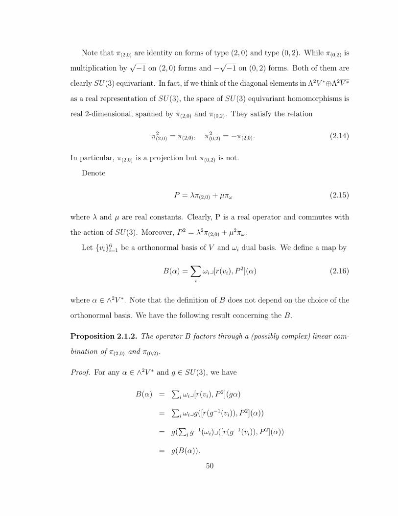
Note that π(2,0) are identity on forms of type (2, 0) and type (0, 2). While π(0,2) is

multiplication by√−1 on (2, 0) forms and −

√−1 on (0, 2) forms. Both of them are

clearly SU(3) equivariant. In fact, if we think of the diagonal elements in Λ2V ∗⊕Λ2V ∗

as a real representation of SU(3), the space of SU(3) equivariant homomorphisms is

real 2-dimensional, spanned by π(2,0) and π(0,2). They satisfy the relation

π2(2,0) = π(2,0), π2

(0,2) = −π(2,0). (2.14)

In particular, π(2,0) is a projection but π(0,2) is not.

Denote

P = λπ(2,0) + µπω (2.15)

where λ and µ are real constants. Clearly, P is a real operator and commutes with

the action of SU(3). Moreover, P 2 = λ2π(2,0) + µ2πω.

Let vi6i=1 be a orthonormal basis of V and ωi dual basis. We define a map by

B(α) =∑i

ωiy[r(vi), P2](α) (2.16)

where α ∈ ∧2V ∗. Note that the definition of B does not depend on the choice of the

orthonormal basis. We have the following result concerning the B.

Proposition 2.1.2. The operator B factors through a (possibly complex) linear com-

bination of π(2,0) and π(0,2).

Proof. For any α ∈ ∧2V ∗ and g ∈ SU(3), we have

B(α) =∑

i ωiy[r(vi), P2](gα)

=∑

i ωiyg([r(g−1(vi)), P2](α))

= g(∑

i g−1(ωi)y([r(g−1(vi)), P

2](α))

= g(B(α)).

50

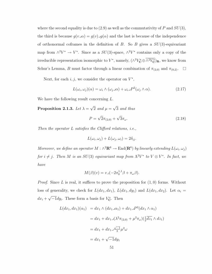
where the second equality is due to (2.9) as well as the commutativity of P and SU(3),

the third is because g(vyα) = g(v)yg(α) and the last is because of the independence

of orthonormal coframes in the definition of B. So B gives a SU(3)-equivariant

map from ∧2V ∗ → V ∗. Since as a SU(3)-space, ∧2V ∗ contains only a copy of the

irreducible representation isomorphic to V ∗, namely, (∧2V ∗C⊕∧2V ∗C)R, we know from

Schur’s Lemma, B must factor through a linear combination of π(2,0) and π(0,2).

Next, for each i, j, we consider the operator on V ∗,

L(ωi, ωj)(α) = ωi ∧ (ωjyα) + ωiyP2(ωj ∧ α). (2.17)

We have the following result concerning L.

Proposition 2.1.3. Let λ =√

2 and µ =√

3 and thus

P =√

2π(2,0) +√

3πω. (2.18)

Then the operator L satisfies the Clifford relations, i.e.,

L(ωi, ωj) + L(ωj, ωi) = 2δij.

Moreover, we define an operator M : ∧2R6 → End(R6) by linearly extending L(ωi, ωj)

for i 6= j. Then M is an SU(3) equivariant map from Λ2V ∗ to V ⊗ V ∗. In fact, we

have

M(β)(v) = vy(−2π1,10 β + πωβ).

Proof. Since L is real, it suffices to prove the proposition for (1, 0) forms. Without

loss of generality, we check for L(dx1, dx1), L(dx1, dy1) and L(dx1, dx2). Let αi =

dxi +√−1dyi. These form a basis for V ∗C. Then

L(dx1, dx1)(α1) = dx1 ∧ (dx1yα1) + dx1yP 2(dx1 ∧ α1)

= dx1 + dx1y(λ2π(2,0) + µ2πω)(12dz1 ∧ dz1)

= dx1 + dx1y√−13µ2ω

= dx1 +√−1dy1

51

because µ2 = 3.

For i = 2, 3

L(dx1, dx1)(αi) = dx1 ∧ (dx1yαi) + dx1yP 2(dx1 ∧ αi)

= 0 + dx1y(λ2π(2,0) + µ2πω)(12(dz1 + dz1) ∧ dzi)

= dx1yλ2 12dz1 ∧ dzi

= λ2

2dzi

= αi

because λ2 = 2. This proves the first equality.

Now consider L(dx1, dy1). We compute

L(dx1, dy1)(α1) = dx1 ∧ (dy1yα1) + dx1yP 2(dy1 ∧ α1)

=√−1dx1 + dy1y(λ2π(2,0) + µ2πω)( −1

2√−1dz1 ∧ dz1)

=√−1dx1 + dx1y

µ2

3

√−1ω

=√−1dx1 − 1

3µ2dx1yω

=√−1dx1 − dy1

=√−1(dz1)

and

L(dy1, dx1)(α1) = dy1 ∧ (dx1ydz1) + dy1yP 2(dx1 ∧ dz1)

= dy1 + dy1y(λ2π(2,0) + µ2πω)(12dz1 ∧ dz1)

= dy1 + dy1yµ2πω(12dz1 ∧ dz1)

= dy1 + dy1yµ2√−13ω

= dy1 −√−1dx1

= −√−1(dx1 +

√−1dy1).

52

Thus

L(dx1, dy1)(α1) + L(dy1, dx1)(α1) = 0.

Also,

L(dx1, dy1)(α2) = dx1 ∧ (dy1ydz2) + dx1yP 2(dy1 ∧ α2)

= 0 + dx1y(λ2π(2,0) + µ2πω)( 12√−1

(dz1 ∧ dz2 − dz1 ∧ dz2))

= −√−1dx1y(dz1 ∧ dz2)

= −√−1dz2

and

L(dy1, dx1)(α2) = dy1 ∧ (dx1ydz2) + dy1yP 2(dx1 ∧ dz2)

= dy1y(λ2π2,0)(12dz1 ∧ dz2)

=√−1dz2.

Thus

L(dx1, dy1)(α2) + L(dy1, dx1)(α2) = 0.

Similarly

L(dx1, dy1)(α3) + L(dy1, dx1)(α3) = 0.

Next we consider L(dx1, dx2).

L(dx1, dx2)(dz1) = dx1 ∧ (dx2ydz1) + dx1yP 2(dx2 ∧ dz1)

= 0 + dx1y(λ2π(2,0) + µ2πω)(12dz2 ∧ dz1 + 1

2dz2 ∧ dz1)

= dx1yλ2π(2,0)(12dz2 ∧ dz1)

= dx1y(dz2 ∧ dz1)

= −dz2

53

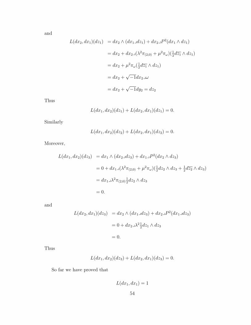
and

L(dx2, dx1)(dz1) = dx2 ∧ (dx1ydz1) + dx2yP 2(dx1 ∧ dz1)

= dx2 + dx2y(λ2π(2,0) + µ2πω)(12dz1 ∧ dz1)

= dx2 + µ2πω(12dz1 ∧ dz1)

= dx2 +√−1dx2yω

= dx2 +√−1dy2 = dz2

Thus

L(dx1, dx2)(dz1) + L(dx2, dx1)(dz1) = 0.

Similarly

L(dx1, dx2)(dz2) + L(dx2, dx1)(dz2) = 0.

Moreover,

L(dx1, dx2)(dz3) = dx1 ∧ (dx2ydz3) + dx1yP 2(dx2 ∧ dz3)

= 0 + dx1y(λ2π(2,0) + µ2πω)(12dz2 ∧ dz3 + 1

2dz2 ∧ dz3)

= dx1yλ2π(2,0)12dz2 ∧ dz3

= 0.

and

L(dx2, dx1)(dz3) = dx2 ∧ (dx1ydz3) + dx2yP 2(dx1ydz3)

= 0 + dx2yλ2 12dz1 ∧ dz3

= 0.

Thus

L(dx1, dx2)(dz3) + L(dx2, dx1)(dz3) = 0.

So far we have proved that

L(dx1, dx1) = 1

54

and

L(dx1, dy1) + L(dy1, dx1) = L(dx1, dx2) + L(dx2, dx1) = 0

. By symmetry and the linearity of L we see that

L(dxi, dxi) = L(dyi, dyi) = 1

,

L(dxi, dxj) + L(dxj, dxi) = 0, i 6= j

and

L(dxi, dyj) + L(dyj, dxi) = 0

. For instance, in order to show

L(dx1, dy2) + L(dy2, dx1) = 0

we replace dx2 by dy2 and dy2 by −dx2. Then it follows from the calculation on

L(dx1, dx2).

Now for arbitray orthonormal basis ωi, the Clifford relations follow from the fact

that the orthogonal transformations act transitively on coframes. If they hold for a

particular coframe, they hold for all.

Suppose g ∈ SU(3). We have for any 1-form α,

L(ωi, ωj)(gα) = ωi ∧ ωjyg(α) + ωiyP 2(ωj ∧ g(α))

= g[(g−1ωi) ∧ (g−1ωj)yα + (g−1ωi)yP 2(g−1(ωj) ∧ α)]

= gL(g−1ωi, g−1ωj)(α).

Now by the definition of M we have for any α = aiωi and β = bjωj,

M(α, β) =1

2(aibj − ajbi)L(ωi, ωj).

55

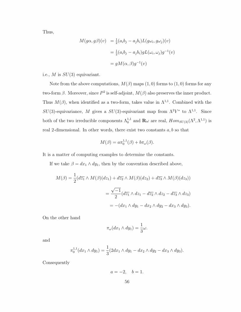
Thus,

M(gα, gβ)(v) = 12(aibj − ajbi)L(gωi, gωj)(v)

= 12(aibj − ajbi)gL(ωi, ωj)g

−1(v)

= gM(α, β)g−1(v)

i.e., M is SU(3) equivariant.

Note from the above computations, M(β) maps (1, 0) forms to (1, 0) forms for any

two-form β. Moreover, since P 2 is self-adjoint, M(β) also preserves the inner product.

Thus M(β), when identified as a two-form, takes value in Λ1,1. Combined with the

SU(3)-equivariance, M gives a SU(3)-equivariant map from Λ2V ∗ to Λ1,1. Since

both of the two irreducible components Λ1,10 and Rω are real, HomSU(3)(Λ

2,Λ1,1) is

real 2-dimensional. In other words, there exist two constants a, b so that

M(β) = aπ1,10 (β) + bπω(β).

It is a matter of computing examples to determine the constants.

If we take β = dx1 ∧ dy1, then by the convention described above,

M(β) =1

2(dz1 ∧M(β)(dz1) + dz2 ∧M(β)(dz2) + dz3 ∧M(β)(dz3))

=

√−1

2(dz1 ∧ dz1 − dz2 ∧ dz2 − dz3 ∧ dz3)

= −(dx1 ∧ dy1 − dx2 ∧ dy2 − dx3 ∧ dy3).

On the other hand

πω(dx1 ∧ dy1) =1

3ω.

and

π1,10 (dx1 ∧ dy1) =

1

3(2dx1 ∧ dy1 − dx2 ∧ dy2 − dx3 ∧ dy3).

Consequently

a = −2, b = 1.

56

Thus M is of the desired form.

2.1.2 Dimension 7

Now we assume that dimV = 7 and we pick an oriented orthonormal basis for V ∗

denoted by dx1, dy1, dx2, dy2, dx3, dy3, du. For later use, let

dzi = dxi +√−1dyi

and define ω and Ψ as in §2.1. We introduce a special three form

Ω = du ∧ ω + ImΨ= du ∧ (dx1 ∧ dy1 + dx2 ∧ dy2 + dx3 ∧ dy3)

+dx1 ∧ dx2 ∧ dy3 − dy1 ∧ dy2 ∧ dy3

+dy1 ∧ dx2 ∧ dx3 + dx1 ∧ dy2 ∧ dx3.

(2.19)

Due to [7], it is now well-known that the exceptional Lie group G2 may be defined

as the stabilizers of Ω. For this reason, we call Ω the fundamental 3-form. We embed

R6 considered in the last section into V to be the hyperplane du = 0. We also let

SU(3) act on V by identity on the line dxi = dyi = 0 and the standard action on

du = 0. Clearly, SU(3) preserves Ω, so it embeds into G2 as a Lie subgroup.

G2-representations

A good resource on this part is [11]. We recall some basic facts. The standard V ∗ is

irreducible with the highest weight (1, 0). The most important part for us is Λ2V ∗.

It decomposes as the sum of two irreducible pieces V (1,0) ⊕ V (1,1) where V (a,b) is the

irreducible representation of G2 with the highest weight (a, b). The subspace V (1,0)

is 7-dimensional, consisting of 2-forms vyΩ for any v ∈ V ∗. The other one V (1,1) is

isomorphic to the Lie algebra g2.

The space Λ5V ∗ is isomorphic to Λ2 as G2-modules either by wedge product

with Ω or by the Hodge star operation. Again the interplay between these two

isomorphisms will be important in defining anti-self-dual instantons in dimesion 7.

57

Hodge star

We only consider the Hodge star on Λ2. Now we may compute that

∗ (α) =1

2Ω ∧ (α) (2.20)

for all α ∈ V (1,0) ⊂ Λ2 and that

∗ α = −Ω ∧ α (2.21)

for α ∈ g2. These may be checked for special forms (e. g., α = duyΩ ∈ V (1,0) and

α = dz1∧dz2 ∈ su(3) ⊂ g2). Then, since these spaces are irreducible and both * and

Ω∧ commutes with G2 action, we know these relations must be true for the whole

spaces. Thus, these irreducible subspaces are indexed by the eigenvalues of ∗(Ω∧).

2.2 Anti-self-dual instantons on nearly Kahler 6-manifolds and G2-cones

Let G be a compact Lie group. Suppose Xn is a smooth manifold endowed with an

(n-4)-form Υ (for our purposes, X = M is nearly Kahler and Υ is the (1, 1)-form ω,

or X = N has G2 holonomy and Υ is the fundamental 3-form Ω). Suppose also Υ is

a (n-4)-form on M and P is a principal G-bundle over X. A connection A on P is

called Υ-instanton if its curvature FA satisfies

Υ ∧ FA = − ∗X FA. (2.22)

Remark 2.2.1. When G is a unitary group, our definition is different from the one

used in [27] (see Remark 1 in its §1.2, however). When G is a special unitary group,

these two definitions coincide. This is the group we will use mostly.

58

Note that if Υ is closed, an Υ-instanton A is Yang-Mills, i.e., it satisfies the

Euler-Lagrange equation of the Yang-Mills functional, since

dA ∗X F = −dΥ ∧ F ±Υ ∧ dAF = 0

because of the Bianchi identity. Thus, an Ω-instanton on a manifold with holonomy

in G2 is Yang-Mills since Ω is closed. Remarkably, as we will show later, when

X = M is nearly Kahler, although ω is not closed, an ω-anti-self-dual instanton is

still Yang-Mills.

2.2.1 Nearly Kahler 6-manifolds

In this subsection, we collect basic facts about nearly Kahler 6-manifolds. The

concept was first introduced and studied by A. Gray in [18]. Later on, N. Hitchin

[22] found that it is a critical point of a diffeomorphism invariant functional and thus

put it in a more natural context.

An SU(3) structure on a 6-manifold M is a reduction of the total coframe bundle

to an SU(3) subbundle. It may be specified by a real two-form ω of type (1, 1) and

a (3, 0)-form Ψ normalized so that 16ω3 = i

8Ψ ∧ Ψ. A nearly Kahler structure is an

SU(3)-structure for which

dω = 3cImΨ, dΨ = 2cω2. (2.23)

for some real constant c.

When c = 0, the underlying almost complex structure is integrable. In fact, M

is Calabi-Yau. When c 6= 0, by scaling the metric, we can always assume c = 1. In

this situation, M is usually called strictly nearly Kahler. In this chapter, we assume

from now on that c = 1 and we speak of this as nearly Kahler without danger of

confusion.

59

Structure equations

Let αi, i = 1, · · · , 3 be a local special unitary coframe, i.e., αi is complex linear and

ω =

√−1

2(α1 ∧ α1 + α2 ∧ α2 + α3 ∧ α3), Ψ = α1 ∧ α2 ∧ α3.

There exists a unique su(3)-valued 1-form (κij) so that

dαi = −κij ∧ αj + εijkαj ∧ αk (2.24)

where summation is understood when repeated barred and unbarred indices appear.

Differentiate this and we get the curvature of κ:

dκij + κik ∧ κkj =1

4(3αi ∧ αj − δijαl ∧ αl) +Kijpqαq ∧ αp, (2.25)

where Kijpq = Kpjiq = Kiqpj = Kjiqp and Kiipq = 0.

It follows from the structure equations that κ is a pseudo-Hermitian-Yang-Mills

connection on the complex tangent bundle of M .

Compact nearly Kahler examples include the standard S6, the flag manifold

SU(3)/T 2, S3 × S3, and CP3 (with an unusual almost complex structure). All

these examples are homogeneous. On the other hand, it remains open to find non-

homogeneous compact examples.

Example 2.2.2 (G2-invariant S6). The standard G2 invariant almost complex struc-

ture on S6 is perhaps the best known non-integrable almost complex structure. As

a subgroup of SO(7), G2 acts transitively on S6 and the stabilizer of any point is

isomorphic to SU(3) ⊂ G2. Thus, G2 preserves an SU(3)-structure on S6. This

SU(3) structure is in fact nearly Kahler. Using Maurer-Cartan forms on G2, we

write the nearly Kahler structure equations

dαi = −κij ∧ αj + εijkαj ∧ αk (2.26)

dκij + κik ∧ κkj =1

4(3αi ∧ αj − δijαl ∧ αl). (2.27)

60

2.2.2 G2-cones over a nearly Kahler 6-manifold

A G2-structure on a 7-manifold N7 is a reduction of the total coframe bundle to

a G2-subbundle. Suppose N7 has such a G2 structure. Then, on N , there exists

a fundamental 3-form Ω characterized by the property that at each point x, there

exists a linear isomorphism u : TxN → R7 so that Ωx = u∗(Ω0). Conversely, given

such a fundamental 3-form Ω on N , the set of such linear isomorphisms forms a G2

subbundle of the total coframe bundle and thus defines a G2-structure on N .

Associated with any G2-structure, N has a metric g. The Levi-Civita connection

of g has its holonomy group contained in G2 if and only if dΩ = d(∗Ω) = 0. R.

Bryant constructed the first metric with holonomy G2 [7]. It was the cone metric

over R+ × SU(3)/T 2. It is now well-known that if M5 is nearly Kahler with the

metric gM , the cone metric on N = R+ ×M6 defined as

gN = dt2 + t2gM

has holonomy in G2. The fundamental 3-form is

Ω = t2dt ∧ ω + t3ImΨ.

Such conical G2-singularities were used by string physicists recently to construct

string models with chiral matter fields (see [2], [1]). For us, the case M = S6 is

especially important. Then the cone has a removable singularity and in fact N = R7.

When studying anti-self-dual instantons on manifolds with G2 holonomy, R7 plays

the natural role of an infinitesimal model.

Hodge star on 2-forms

Suppose ωi(i = 1, · · · , 6) is an oriented local orthonormal coframe for M . Then,

dt, tωi(i = 1, · · · , 6) form an oriented local orthonormal coframe for the cone N .

61

Denote ∗M and ∗N Hodge star operations on M and N respectively. It is easy to

show that

t2dt ∧ ∗M(ωi ∧ ωj) = ∗N(ωi ∧ ωj)

and

∗N(dt ∧ ωi) = t4 ∗M (ωi).

Consequently, if a 2-form α on N satisfies ∂∂tyα = 0, its Hodge star may be computed

by

∗N α = t2dt ∧ ∗M(α), (2.28)

and if α = dt ∧ β with ∂∂tyβ = 0,

∗N (dt ∧ β) = t4 ∗M (β), (2.29)

where we extend ∗M linearly across functions on N . The formula (2.28), (2.29) will

be important below.

2.2.3 ω anti-self-dual instantons

If the underlying manifold is almost Hermitian with the Kahler form ω, we may

decompose the curvature as

F = F 2,0 + F 2,0 + (F )1,1 +Hω,

where F 2,0 is of type (2, 0) and (F )1,1 is of type (1, 1) but with zero ω-trace. Now

the ω-anti-self-dual instanton condition (2.22) implies F 2,0 = H = 0.

Remark 2.2.3. In the case G is a special unitary group, the above argument implies

that an ω-instanton is the same as a pseudo-Hermitian-Yang-Mills connection on the

canonically associated complex vector bundle.

If, moreover, we are working on a nearly Kahler manifold, this condition may be

simplified.

62

Lemma 2.2.4. Suppose A is a connection on nearly Kahler M6 and F is its curva-

ture. The following are equivalent:

a. F ∧ ImΨ = 0.

b. F ∧Ψ = 0.

c. F ∧ ReΨ = 0.

d. A is an ω-anti-self-dual instanton.

Consequently, if F is of type (1, 1), A is an ω-anti-self-dual instanton.

Proof. 1. a=⇒b. We write F = F 2,0 + F 2,0 + (F )1,1 + Hω. Then F ∧ ImΨ = 0

gives

F ∧ (Ψ−Ψ) = 0,

i.e.,

F 2,0 ∧Ψ = 0.

It follows then that

F ∧Ψ = 0

and hence F ∧Ψ = 0.

2. b=⇒c is obvious.

3. c=⇒d. As mentioned before, A is ω-anti-self-dual if and only if F 2,0 = 0 and

H = 0 in the above decomposition. Now

F ∧ ReΨ =1

2F ∧ (Ψ + Ψ) =

1

2F 2,0 ∧Ψ + F 2,0 ∧Ψ.

63

Thus c gives F 2,0 = 0. Differentiating c gives

0 = dA(F ∧ ReΨ)

= dAF ∧ ReΨ + F ∧ dReΨ

= 0 + 2F ∧ ω2

= 2Hω3

where the last equality uses (2.23) and the Bianchi identity. Hence

H = 0.

4. d=⇒a is obvious.

This lemma says that we could have defined an ω-anti-self-dual as F 2,0 = 0.

This reduces the indeterminacy and will be useful later when we construct concrete

examples.

Remark 2.2.5. The same result holds for a more general class of almost complex

manifolds, called strictly quasi-integrable in [4]. We leave it for the reader to carry

out the details. In fact, this has already been observed in [4] for unitary instantons.

Generality

We now address the problem of the involutivity problem of the instanton equations.

First, the instanton equations may be rephrased as

F ∧Ψ = 0 (2.30)

and

F ∧ ω2 = 0. (2.31)

64

Since the problem is local, we assume that the bundle is trivial, and the connection

is simply a g-valued 1-form A. The differential system we need to analyze is

I = 〈F ∧Ψ, F ∧ ω2〉,

defined on M × g where F = dA+ 12[A,A]. We have

Lemma 2.2.6. The system I is involutive with Cartan characters

(s0, s1, s2, s3, s4, s5, s6) = (0, 0, 0, 0, 2d, 3d, d).

where d = dimG.

Proof. Note that

d(F ∧Ψ) = [A,F ] ∧Ψ + F ∧ dΨ ≡ 0, mod I.

because of Bianchi identity and the nearly Kahler condition dΨ = 2ω2. It is now

routine to check the system is involutive with displayed characters.

Some remarks are in order.

Remark 2.2.7. More generally, Lemma 2.2.6 holds for similarly defined ω-instantons

on a quasi-integrable U(3)-structure (see [4] for the definition). We leave the details

for the interested readers. When G = U(r) is a unitary group, it is treated in [4] .

Remark 2.2.8. For nearly Kahler M , we could have used the differential system

〈F ∧ ImΨ〉 by Lemma 2.2.4. The reader can check that this is involutive with the

last Cartan character also equal to d. The advantage of the original system is that it

applies to more general almost complex manifolds.

Remark 2.2.9. The last character is d, due to the fact that gauge transformations

depend on d functions of 6 variables and that instanton equations are gauge-invariant.

We leave for the interested reader to impose a symmetry breaking condition.

65

Instantons are Yang-Mills

Now we compute

dA ∗M F = −dω ∧ F − ω ∧ dAF = −3ImΨ ∧ F = 0

because F is of type (1, 1).

Proposition 2.2.10. An ω-instanton on a nearly Kahler 6-manifold is Yang-Mills.

A consequence is some removable singularity results for instantons on nearly

Kahler 6-manifolds.

Corollary 2.2.11. Suppose that all representations of π1(M) → G are trivial and

that E is a trivial smooth bundle over M . Assume that A is a ω-instanton on E with

a closed singular set S whose n − 4 Hausdorff measure is locally finite. Then there

exists ε = ε(G,M) such that if

‖ FA ‖∞≤ ε,

then the singularity of A is removable.

Corollary 2.2.12. Suppose that all representations of π1(M) → G are trivial and

that E is a trivial smooth G bundle over M . Assume that A is a ω-instanton on E

whose singular set is a closed smooth submanifold of codimension at least 4. Then

there exists ε = ε(G,M) such that if

‖ FA ‖L 62 (M)≤ ε,

then the singularity of A is removable.

Both are proved by employing the results in [29].

66

Instantons as critical points of a Chern-Simons functional

Consider the functional

CS(A) =

∫M

tr(F 2A) ∧ ω. (2.32)

On a Kahler manifold, since ω is closed, CS is a topological constant. However, on

a nearly Kahler manifold, this gives more interesting information.

It is easy to compute that the first variation of CS is

δCS = 2

∫M

tr(FA ∧ dAδA) ∧ ω.

Integration by parts gives

δCS = 2

∫M

tr[dA(FA ∧ ω) ∧ δA].

Thus the Euler-Lagrange equation for CS is

dA(FA ∧ ω) = 0.

Using Bianchi Identity, we see this is equivalent to

F ∧ ImΨ = 0. (2.33)

It follows from Lemma 2.2.4 that

Proposition 2.2.13. An ω-anti-self-dual instanton is equivalent to a critical con-

nection of the Chern-Simons functional CS.

This makes it possible to use variational methods to study ω-anti-self-dual in-

stantons on nearly Kahler 6-manifolds.

It also follows that the gradient flow of CS takes the form

d

dtA = ∗M(F ∧ ImΨ). (2.34)

67

Remark 2.2.14. To illustrate, we assume that the principal bundle under consider-

ation is topologically trivial. Using dω = 3ImΨ and transgression formula, it can be

shown that up to a constant

CS(A) =

∫M

tr(F ∧ A− 1

3A ∧ A ∧ A) ∧ ImΨ. (2.35)

Here we regard G as a matrix Lie group. This formulation is more similar to the

Chern-Simons functional on 3-manifolds.

Next we compute the second variation Q of CS. Suppose that A(s, t) (for small

s, t) are a two parameter family of connections such that A = A(0, 0) is an instanton.

Let a = ∂A∂s|s=0,t=0, b = ∂A

∂t|s=0,t=0.Then by definition

Q(a, b) =∂2

∂s∂t|s=0,t=0CS(A)

We have essentially computed that

∂

∂tCS(A) = −6

∫M

tr(FA ∧ ImΨ ∧ ∂

∂tA(s, t)).

Thus the second derivative is (remember FA ∧ ImΨ = 0)

Q(a, b) = −6

∫M

tr(dA(∂A

∂s|s=0,t=0) ∧ ImΨ ∧ ∂A

∂t|s=0,t=0) (2.36)

= −6

∫M

tr(dAa ∧ ImΨ ∧ b) (2.37)

Clearly, this is a symmetric bilinear form.

The null space of Q consists of a so that

dAa ∧ ImΨ = 0.

This implies dAa is of type (1, 1) and hence

dAa ∧Ψ = 0.

68

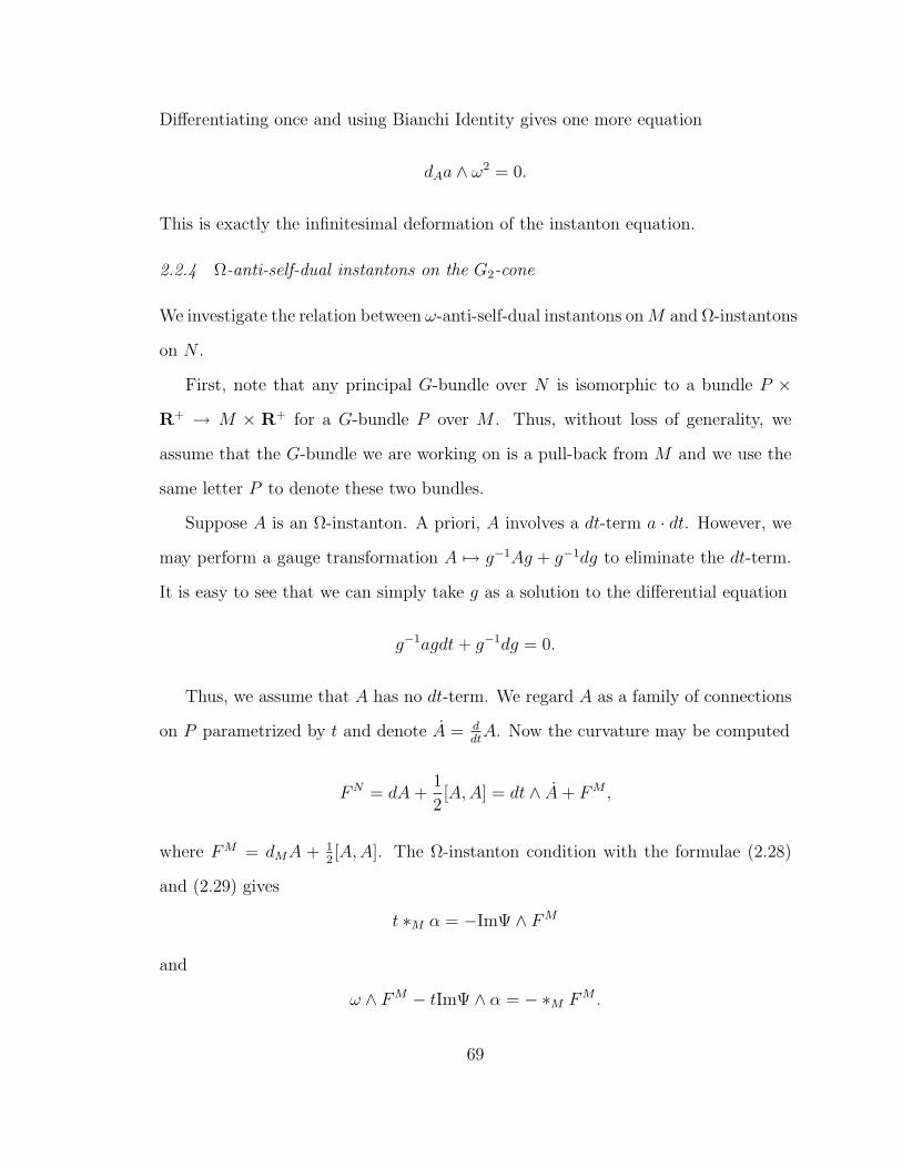
Differentiating once and using Bianchi Identity gives one more equation

dAa ∧ ω2 = 0.

This is exactly the infinitesimal deformation of the instanton equation.

2.2.4 Ω-anti-self-dual instantons on the G2-cone

We investigate the relation between ω-anti-self-dual instantons onM and Ω-instantons

on N .

First, note that any principal G-bundle over N is isomorphic to a bundle P ×

R+ → M × R+ for a G-bundle P over M . Thus, without loss of generality, we

assume that the G-bundle we are working on is a pull-back from M and we use the

same letter P to denote these two bundles.

Suppose A is an Ω-instanton. A priori, A involves a dt-term a · dt. However, we

may perform a gauge transformation A 7→ g−1Ag + g−1dg to eliminate the dt-term.

It is easy to see that we can simply take g as a solution to the differential equation

g−1agdt+ g−1dg = 0.

Thus, we assume that A has no dt-term. We regard A as a family of connections

on P parametrized by t and denote A = ddtA. Now the curvature may be computed

FN = dA+1

2[A,A] = dt ∧ A+ FM ,

where FM = dMA + 12[A,A]. The Ω-instanton condition with the formulae (2.28)

and (2.29) gives

t ∗M α = −ImΨ ∧ FM

and

ω ∧ FM − tImΨ ∧ α = − ∗M FM .

69

We denote the (1, 1)-part (with coefficients depending on t) of FM by FM0 and FM

1 =

FM − FM0 . By type decomposition in the above two equations we have

t ∗M A = −ImΨ ∧ FM1 ,

ω ∧ FM0 = − ∗M FM

0 , (2.38)

and

ω ∧ FM1 − tImΨ ∧ A = − ∗M FM

1 .

By taking Hodge star of both sides, we see that the first equation is equivalent to

tA = ∗(ImΨ ∧ FM1 ). (2.39)

Combining (2.8) and (2.5) we see that the last equation is implied by (2.39).

The equation (2.38) looks very much like the ω-anti-self-dual instanton equation

on M . The only problem is that FM0 is not necessarily the curvature of a well-defined

connection.

The equation (2.39) is exactly the gradient flow of the Chern-Simons functional

CS. It would be interesting to analyze this equation coupled with (2.38). The first

natural question is whether we could evolve through (2.39) in the class of ω-anti-

self-dual instantons on M to get a Ω-anti-self-dual instanton on N . Unfortunately,

this is impossible. An ω-instanton has its curvature of type (1, 1). If A(t) stays

ω-anti-self-dual for all t, the evolution equation (2.39) will imply that ddtA = 0, i.e.,

A is constant in t. On the other hand, if A is constant in t and ω-anti-self-dual,

it is Ω-anti-self-dual when pulled back to the cone N . These give a class of special

solutions.

Lemma 2.2.15. Suppose A is an ω-anti-self-dual connection on the nearly Kahler

6-manifold M and extend it to the G2-cone N by constant in t. Then A is a Ω-anti-

self-dual connection on N .

70

Remark 2.2.16. When M = S6, in order that the principal bundle extend through

the origin in R7, P has to be trivial over M . Even when this is true, the extended

Ω-anti-self-dual connection on R7 \ 0 described in the above Lemma does not nec-

essarily extend through origin. It is interesting to ask under what condition this

singularity is removable after a gauge transformation.

2.3 A Weitzenbock formula

In this section, we derive a Weitzenbock formula for nearly Kahler 6-manifolds and

describe its application to the deformation of ω-anti-self-dual instantons.

2.3.1 The general formula

Let E be a vector bundle over M . Suppose E is equipped with a metric and a metric-

compatible connection A. Suppose also that the curvature FA is an ω-instanton.

Consider the following complex

0→ Γ(E)dA−→ Γ(E ⊗ T ∗M)

PdA−→ Γ(E ⊗ (Λ(2,0)T ∗M)R ⊕Rω),

where the operator dA is induced from d and the connection A and P is defined in

§2.1.1 the projection onto the orthogonal complement of ω-trace free (1, 1)-forms.

This complex is elliptic at the middle term. It could be extended to an elliptic

complex, but we will not need the full sequence.

The 0th cohomology group consists of parallel sections of E. We are mainly

interested in the 1st cohomology group. A well-known result in Hodge Theory states

that this group can be represented by harmonic sections, i.e., the kernel of the elliptic

operator

∆A = (d∗A + PdA)∗(d∗A + PdA) = dAd∗A + d∗AP

2dA

71

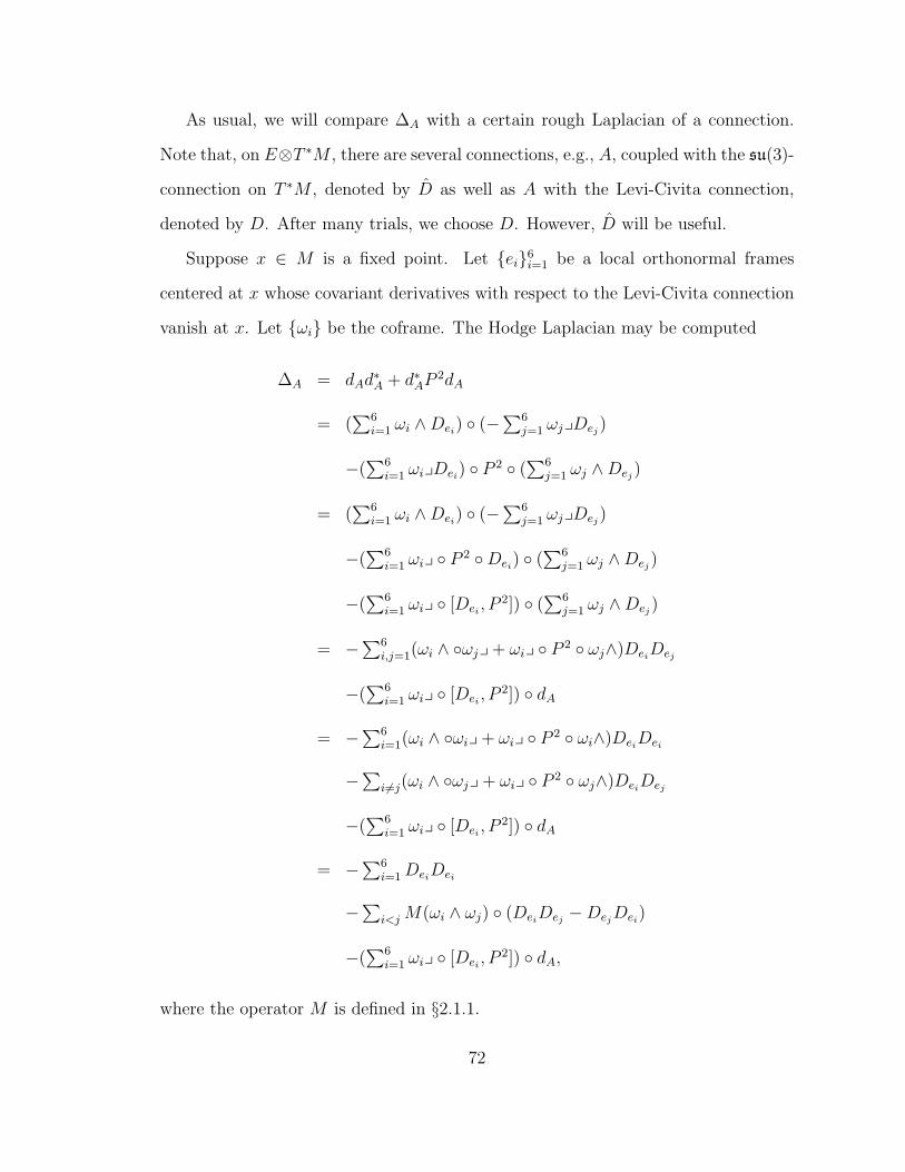
As usual, we will compare ∆A with a certain rough Laplacian of a connection.

Note that, on E⊗T ∗M , there are several connections, e.g., A, coupled with the su(3)-

connection on T ∗M , denoted by D as well as A with the Levi-Civita connection,

denoted by D. After many trials, we choose D. However, D will be useful.

Suppose x ∈ M is a fixed point. Let ei6i=1 be a local orthonormal frames

centered at x whose covariant derivatives with respect to the Levi-Civita connection

vanish at x. Let ωi be the coframe. The Hodge Laplacian may be computed

∆A = dAd∗A + d∗AP

2dA

= (∑6

i=1 ωi ∧Dei) (−

∑6j=1 ωjyDej

)

−(∑6

i=1 ωiyDei) P 2 (

∑6j=1 ωj ∧Dej

)

= (∑6

i=1 ωi ∧Dei) (−

∑6j=1 ωjyDej

)

−(∑6

i=1 ωiy P 2 Dei) (

∑6j=1 ωj ∧Dej

)

−(∑6

i=1 ωiy [Dei, P 2]) (

∑6j=1 ωj ∧Dej

)

= −∑6

i,j=1(ωi ∧ ωjy+ ωiy P 2 ωj∧)DeiDej

−(∑6

i=1 ωiy [Dei, P 2]) dA

= −∑6

i=1(ωi ∧ ωiy+ ωiy P 2 ωi∧)DeiDei

−∑

i 6=j(ωi ∧ ωjy+ ωiy P 2 ωj∧)DeiDej

−(∑6

i=1 ωiy [Dei, P 2]) dA

= −∑6

i=1DeiDei

−∑

i<jM(ωi ∧ ωj) (DeiDej−Dej

Dei)

−(∑6

i=1 ωiy [Dei, P 2]) dA,

where the operator M is defined in §2.1.1.

72

Recall Dei|x = 0. Thus at x,

−6∑i=1

DeiDei

= D∗D

the rough Laplacian. For the same reason, DeiDej− Dej

Deiis the curvature on

T ∗M ⊗ E. The curvature has two parts R ⊗ IdE + IdT ∗M ⊗ FE where R is the

Riemannian curvature of M . We write R = 14Rklijωl ∧ ωk ⊗ ωi ∧ ωj. Given a 1-form

α and two vectors X and Y

DXDY α−DYDXα−D[X,Y ]α =1

4Rklijωi ∧ ωj(X, Y )αy(ωl ∧ ωk).

Now consider the term in the formula∑6

i=1 ωiy [Dei, P 2]. Note that the su(3)-

connection D commutes with P 2, i.e., [Dei, P 2] = 0 for any ei. Moreover, the dif-

ference r(ei) = Dei− Dei

is exactly the su(3)-torsion up to a constant. Here, the

nearly Kahler structure plays the central role. By definition, this torsion r is covari-

antly constant with respect to the su(3)-connection. Hence, r satisfies (2.9) and the

operator

6∑i=1

ωiy [Dei, P 2] =

6∑i=1

ωiy [r(ei), P2] = B

factors through a linear combination of π(2,0) and π(0,2) according to (2.1.2).

In summary, we have the following Weitzenbock formula.

∆A = ∇∗A∇A (2.40)

−B dA (2.41)

−1

2

∑i,j

M(ωi ∧ ωj) Rij ⊗ IdE −1

2

∑ij

M(ωi ∧ ωj)⊗ Fij. (2.42)

A routine consequence of this formula is the following:

73

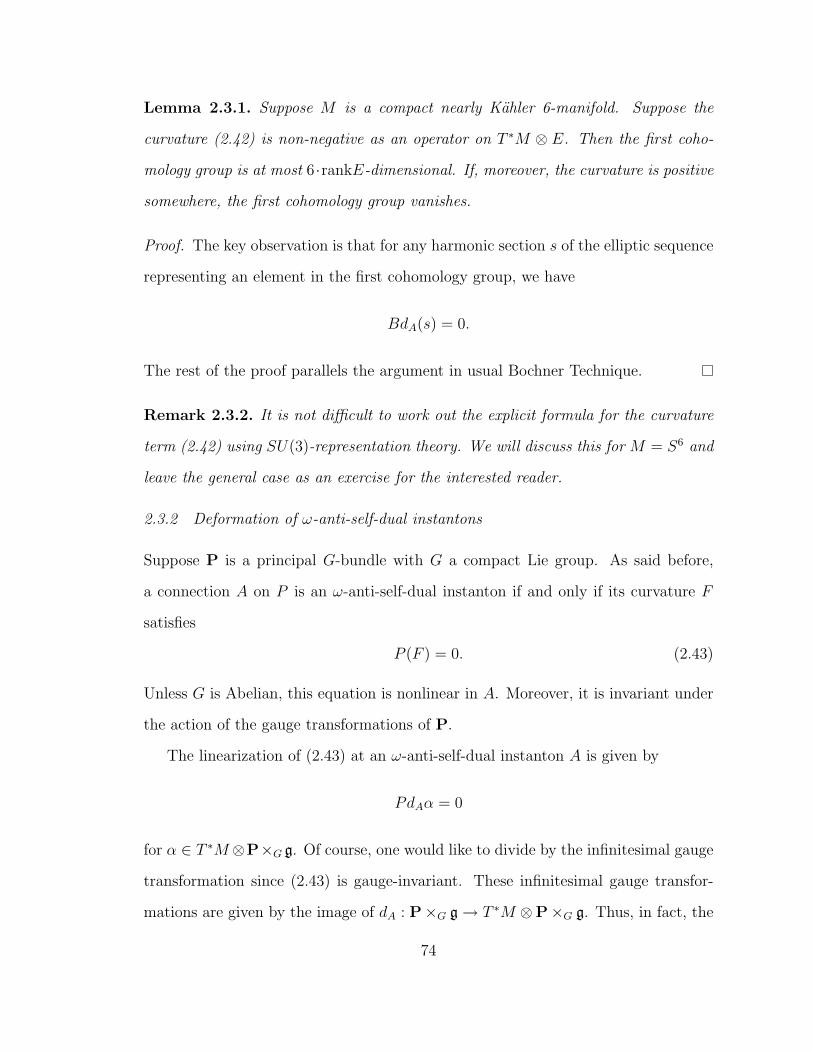
Lemma 2.3.1. Suppose M is a compact nearly Kahler 6-manifold. Suppose the

curvature (2.42) is non-negative as an operator on T ∗M ⊗ E. Then the first coho-

mology group is at most 6·rankE-dimensional. If, moreover, the curvature is positive

somewhere, the first cohomology group vanishes.

Proof. The key observation is that for any harmonic section s of the elliptic sequence

representing an element in the first cohomology group, we have

BdA(s) = 0.

The rest of the proof parallels the argument in usual Bochner Technique.

Remark 2.3.2. It is not difficult to work out the explicit formula for the curvature

term (2.42) using SU(3)-representation theory. We will discuss this for M = S6 and

leave the general case as an exercise for the interested reader.

2.3.2 Deformation of ω-anti-self-dual instantons

Suppose P is a principal G-bundle with G a compact Lie group. As said before,

a connection A on P is an ω-anti-self-dual instanton if and only if its curvature F

satisfies

P (F ) = 0. (2.43)

Unless G is Abelian, this equation is nonlinear in A. Moreover, it is invariant under

the action of the gauge transformations of P.

The linearization of (2.43) at an ω-anti-self-dual instanton A is given by

PdAα = 0

for α ∈ T ∗M⊗P×G g. Of course, one would like to divide by the infinitesimal gauge

transformation since (2.43) is gauge-invariant. These infinitesimal gauge transfor-

mations are given by the image of dA : P×G g→ T ∗M ⊗P×G g. Thus, in fact, the

74

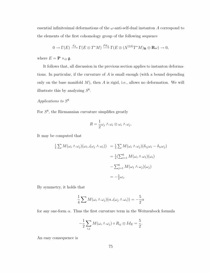
essential infinitesimal deformations of the ω-anti-self-dual instanton A correspond to

the elements of the first cohomology group of the following sequence

0→ Γ(E)dA−→ Γ(E ⊗ T ∗M)

PdA−→ Γ(E ⊗ (Λ(2,0)T ∗M)R ⊕Rω)→ 0,

where E = P×G g.

It follows that, all discussion in the previous section applies to instanton deforma-

tions. In particular, if the curvature of A is small enough (with a bound depending

only on the base manifold M), then A is rigid, i.e., allows no deformation. We will

illustrate this by analyzing S6.

Applications to S6

For S6, the Riemannian curvature simplifies greatly

R =1

2ωj ∧ ωi ⊗ ωi ∧ ωj.

It may be computed that

14

∑M(ωi ∧ ωj)(ω1y(ωj ∧ ωi)) = 1

4

∑M(ωi ∧ ωj)(δ1jωi − δ1iωj)

= 14(∑6

i=1M(ωi ∧ ω1)(ωi)

−∑6

j=1M(ω1 ∧ ωj)(ωj)

= −52ω1.

By symmetry, it holds that

1

4

∑M(ωi ∧ ωj)(αy(ωj ∧ ωi)) = −5

2α

for any one-form α. Thus the first curvature term in the Weitzenbock formula

−1

2

∑i,j

M(ωi ∧ ωj) Rij ⊗ IdE =5

2.

An easy consequence is

75

Theorem 2.3.3. A flat ω-instanton on S6 is rigid.

As another application, we consider the su(3)-connection on the standard struc-

ture bundle G2 → S6. We need to describe the su(3) connection a bit. Recall the

connection 1-form κij in (2.26). Through this, the connection on (1, 0)-forms is

DXαi = −αjκij(X)

for any vector field X. Correspondingly the curvature is give by

DXDY −DYDX −D[X,Y ](αi) = −αj(dκij + κik ∧ κkj)(X, Y ).

Thus the action of F on (1, 0) forms is given by

αi 7→ −αj ⊗ (dκij + κik ∧ κkj).

More generally,

F : α 7→ αy− 1

2(αi ∧ αj)⊗ (dκij + κik ∧ κkj).

Denote Ωij = dκij + κik ∧ κkj = 14(3αi ∧ αj − δijαl ∧ αl). For each k, l, Fkl in the

curvature term is

Fkl : α 7→ αy− 1

2(αi ∧ αj)Ωij(ek, el).

Then the second curvature term in this context when E = T 1,0 is

−1

2M(ωk ∧ ωl)(v)⊗ Fkl(α)

= −1

2M(ωk ∧ ωl)(v)⊗ αy(−1

2)(αi ∧ αj)Ωij(ek, el)

=1

4M(Ωij)(v)⊗ αy(αi ∧ αj)

= −1

2vyΩij ⊗ αy(αi ∧ αj)

76

because Ωij is in Λ1,10 . This is not exactly what we want when we study the deforma-

tion of su(3) connection on G2. However, all we need is to replace α by a section of

adG2 ' Λ1,10 where the identification has been defined before. The action of αi ∧ αj

will be the Lie bracket whose meaning should be clear via the aforementioned iden-

tification.

Denote

B(s, t) = 〈−1

2M(ωi, ωj)⊗ Fij(s), t〉

where s, t are sections of T ∗ ⊗ adG2 . Note that if s = φ⊗X and t = ψ ⊗ Y we have

B(s, t) = −1

2〈M(ωi ∧ ωj)(φ)⊗ [Fij, X], ψ ⊗ Y 〉

= −1

2〈M(ωi ∧ ωj)(φ), ψ〉〈[Fij, X], Y 〉

= −1

2〈M(ωi ∧ ωj), φ ∧ ψ〉〈Fij, [X, Y ]]〉

= 〈−1

2M(ωi ∧ ωj)⊗ Fij, [s, t]〉.

where we view M(ωi ∧ ωj) as a 2-form.

Then since F is SU(3)-invariant, B is a SU(3)-invariant symmetric bilinear form

on R6 ⊗ su(3). We study the space of SU(3) invariant symmetric bilinear forms on

R6 ⊗ u(3). One candidate is obvious, the SU(3) invariant inner product, denoted

by B0. For others we apply representation theory of SU(3). Then complexified

representation (R6 ⊗ su(3))⊗C ∼= (C3 ⊕C3)⊗C sl3(C) decomposes as

(V (1,0) ⊕ V (1,0))⊕ V (2,0) ⊕ V (2,0) ⊕ V (2,1) ⊕ V (2,1),

where V (a,b) denotes the irreducible complex representation of SU(3) with the highest

weight (a, b). The representation V (a,b) is real (i.e., V (a,b) ∼= V (a,b)) if and only if a = b.

Thus the original R6 ⊗ u(3) decomposes as

(V (1,0))R ⊕ (V (2,0))R ⊕ (V (2,1))R,

77

where VR means the real representation by forgetting the complex structure of V .

The irreducible pieces are 6, 12, 30 dimensional respectively. One of them is known

as V (1,0) = C3. Coupled with the standard inner product, every SU(3)-invariant

bilinear form on R6 ⊗ u(3) will give rise to a SU(3)-invariant endomorphism. The

space of such endomorphisms is 6 dimensional, 2 for each irreducible component.

Of the two independent bilinear forms on every irreducible component, one can be

taken as the SU(3)-invariant inner product and the other is symplectic. Thus the

space of SU(3)-invariant symmetric bilinear forms is 3-dimensional, represented by

linear combinations of inner products of various components.

We will construct a basis for this 3-dimensional space. We already have one–

the inner product of the whole space B0. To construct two more, we need more

information about the irreducible components.

First consider the map

T1 : R6 ⊗ su(3)→ R6

defined by v ⊗ α 7→ vyα. This map is clearly SU(3)-equivariant so B1(u, v) =

〈T1u, T1v〉 is clearly SU(3)-invariant. Moreover, since R6 ⊗ su(3) contains only one

copy of R6 and T1 is nonzero, by Schur’s Lemma, T1 and thus B1 is zero on (V (2,0))R⊕

(V (2,1))R.

For later estimate, we need the right inverse of T1. Define the operatore

S1 : R6 → R6 ⊗ su(3)

by

v → 3

16

∑i

αi ⊗ π1,10 (αi ∧ v) +

3

16

∑i

αi ⊗ π1,10 (αi ∧ v).

It is clearly SU(3) equivariant. Since R6 is irreducible, S1 maps onto the irreducible

components V(1,0)R ∈ R6 ⊗ su(3).

78

Then the composition T1S1 must be a linear combination of Id and J(the almost

complex structure). However, it may be computed that

S1(α1) =3

16(α1 ⊗ π1,1

0 (α1 ∧ α1) + α2 ⊗ π1,10 (α2 ∧ α1) + α3 ⊗ π1,1

0 (α3 ∧ α1)

=3

16(α1 ⊗

1

3(2α1 ∧ α1 + α2 ∧ α2 + α3 ∧ α3) + α2 ⊗ α2 ∧ α1 + α3 ⊗ α3 ∧ α1)

Thus T1S1(α1) = α1 and hence T1S1 = Id.

Meanwhile, it is easy to compute that

B0(S1(α), S1(α)) =3

4B1(S1(α), S1(α)). (2.44)

Second consider the map

T2 : R6 ⊗ su(3)→ ∧3R6 → (R6 ∧ ω)⊥.

defined by v⊗α 7→ v∧α followed by the projection onto the orghogonal complement

of R6 ∧ ω. Define B2(u, v) = 〈T2u, T2v〉. Then T2 is SU(3) equivariant and B2 is

SU(3) invariant. The image of T2 lies in the space of type (2, 1) + (1, 2) forms.

We also need the partial inverse of T2. Define

S2 : ψ 7→ 1

4(αi ⊗ π1,1

0 (αiyψ) + αi ⊗ π1,10 (αiyψ)).

It is clearly SU(3) equivariant. The image under S2 of (2, 1)+(1, 2) forms orthogonal

to R6 ∧ ω is V (2,0). It is easy to compute

S2(α1 ∧ α2 ∧ α3) =1

4(2α1 ⊗ α2 ∧ α3 − 2α2 ⊗ α1 ∧ α3).

Consequently, T2S2(α1 ∧ α2 ∧ α3) = α1 ∧ α2 ∧ α3. Thus T2S2 = 1.

It is also easy to verify that

B0(S2(ψ), S2(ψ)) =1

2B2(S2(ψ), S2(ψ)). (2.45)

79

On the other hand, it may be computed that

T2S1 = 0, T1S2 = 0. (2.46)

The 3 symmetric bilinear forms B0, B1, B2 are clearly linearly independent. Thus

there exist constants λi such that B = λ0B0 + λ1B1 + λ2B2. We will compute

examples to determine these constants.

Set

u1 = α1 ⊗√−1(2α1 ∧ α1 − α2 ∧ α2 − α3 ∧ α3),

u2 = α1 ⊗ (α2 ∧ α3 + α2 ∧ α3).

and

u3 = α1 ⊗ α1 ∧ α2.

It is easy to see that [u1, u1] = [u2, u2] = 0. Thus

0 = B(u1, u1) = λ0B0(u1, u1) + λ1B1(u1, u1) = (λ0 +4

3λ1)B0(u1, u1),

0 = B(u2, u2) = λ0B0(u2, u2) + λ2B2(u2, u2) = (λ0 + 2λ2)B0(u2, u2),

and

B(u3, u3) = λ0B0(u3, u3).

Hence

λ1 = −3

4λ0, λ2 = −1

2λ0

and

λ0 =B(u3, u3)

B0(u3, u3).

The curvature F = −18(3αi ∧ αj − δijαl ∧ αl)⊗C αi ∧ αj. Thus

B(u3, u3) = 〈F, [u3, u3]〉= 〈F, α1 ∧ α1 ⊗ (−2α1 ∧ α1 + 2α2 ∧ α2)〉= 12.

80

Thus λ0 = 32. Consequently,

B =3

2(B0 −

3

4B1 −

1

2B2).

Lemma 2.3.4.

B ≥ 0.

Proof. Let ψ ∈ R6 ⊗ su(3) be real. Write ψ = S1T1(ψ) + S2T2(ψ) + ψ. Note that

ψ ∈ kerT1 ∩ kerT2. Thus, in fact ψ ∈ V (2,1)R . These three different components are

thus pairwise perpendicular, since they lie in different irreducible pieces. It follows

that

2

3B(ψ, ψ) = B0(ψ, ψ).

The contribution from the second curvature term is nonnegative. All together

the curvature part is strictly positive.

To summarize, we have the following result.

Theorem 2.3.5. The su(3)-connection on G2 → S6 in (2.26) is a rigid SU(3)

instanton.

2.4 SO(4)-invariant examples

We construct cohomogeneity one SU(2)(S3) anti-self-dual instantons (equivalent to

pseudo-Hermitian-Yang-Mills here) on S6. The idea is to impose symmetries to

reduce the instanton equations to ODEs. We regard SU(2) = S3 as the set of

unit quaternions whose Lie algebra is the tangent space at 1 consisting of imaginary

quaternions for which we use I, J,K to denote the standard basis for imaginary

quaternions. A remark on the notation is necessary. Throughout this section, we

use√−1 to represent complex numbers to avoid confusion with quaternions. It

81

should be cautioned that when complex numbers are regarded as coefficients in the

complexified Lie algebra, they commute with I, J,K rather than following the usual

rule of multiplication with quaternions. Hopefully, this will be clear from context.

2.4.1 A dense open subset U of S6

More precisely, U = S6 \ (S2 ∪ S3) is parametrized by S2 × S3 × (0, π2) as

(x, y, t) 7→ v = (x cos t, y sin t))

where we think of x ∈ S3 ⊂ R4 as a unit 4-vector and y ∈ S2 ⊂ R3 as a unit 3-vector.

Actually, if we extend the map to the closed interval [0, π2], we cover the whole S6.

Reverse the picture and we get a map t : S6 → [0, π2] which is roughly the distance

function from the totally geodesic pseudo-holomorphic S2 = t = 0. A generic level

set is a scaled S2 × S3 and t = π2 is a totally geodesic, special Lagrangian S3.

For later use,

S3 × S2 = S3 × S3/S1

as a homogeneous space via (p, q) ∼ (pz, qz) for (p, q) ∈ S3 × S3 and z ∈ S1.

Composing this quotient with the map (x, y, t) 7→ v, we have a map S3×S3×(0, π2)→

U ⊂ S6 by

(p, q) 7→ (pIp cos t, qp−1 sin t).

Denote by ω = ω1I + ω2J + ω3K and ψ = ψ1I + ψ2J + ψ3K the left-invariant

Maurer-Cartan forms on the two copies of S3, respectively. Then, dt, ω2, ω3, ψ2, ψ3

and τ = ω1−ψ1 form a basis of semibasic 1-forms for the projection S3×S3×(0, π2)→

U . We use this to describe the nearly Kahler structures on U induced from S6.

Recall that the G2-invariant almost complex structure J on TvS6 is given by the

left Cayley multiplication by v when we we regard both v and tangent vectors as

Cayley numbers in R8 = O. In other words,

J : dv 7→ v · dv. (2.47)

82

The standard metric and J determines the Kahler 2-form ω = 〈Jdv, dv〉.

Using (2.47) and Cayley-Dickson rule of Cayley multiplication, we can establish

the following

J(dt) = sin tτ,

J(2 cos tω3) = (2 cos2 t− sin2 t)ω2 + sin2 tψ2,

J(−2 cos tω2) = (2 cos2 t− sin2 t)ω3 + sin2 tψ3.

The Kahler form ω is determined by

−ω = 〈v, Jv〉 = 2 sin tψ1 ∧ dt− 2 sin tω1 ∧ dt

+2 cos t(9 cos2 t− 5)ω3 ∧ ω2 + 6 sin2 t cos tω3 ∧ ψ2

−6 cos t sin2 tω2 ∧ ψ3 + 2 sin2 t cos tψ2 ∧ ψ3.

2.4.2 Bundle constructions and SO(4)-invariant connections

S3-bundles

We now describe the principal S3-bundles on which to construct instantons. First,

note that S3 × S3 × (0, π2) → S3 × S2 × (0, π

2) in §2.4.1 is a principal S1-bundle.

The principal S3-bundles are obtained by extending the structure group through the

group homomorphisms

z 7→ zl

for z ∈ S1. More explicitly, denote

Bl = S3 × S3 × S3 × (0,π

2)/ ∼

where

(p, q, r, t) ∼ (pz, qz, rz−l, t)

83

for any (p, q, r, t) ∈ S3×S3×S3× (0, π2), t ∈ (0, π

2) and z ∈ S1. The structure group

S3 acts on Bl by

[p, q, r, t] 7→ [p, q, rg, t]

for any g ∈ S3. Clearly this is well-defined. Then the projection

[p, q, r, t] 7→ (pIp−1 cos t, qp−1 sin t)

makes Bl a principal S3-bundle over U .

Remark 2.4.1 (on the symmetry of Bl). Note that if we let [g1, g2] ∈ SO(4) =

S3 × S3/Z2 act on Bl by

[p, q, r, t]→ [g1p, g2q, r, t]

and on S6 by

(x, y) 7→ (pap−1, qbp−1),

this action commutes with the bundle projection. In other words, the principal bundle

Bl over U has an SO(4)-symmetry. It is well-known that the action on S6 is induced

from the embedding of SO(4) into G2 and has cohomogeneity 1. We will construct

SO(4)-invariant instantons, i.e., instantons of cohomogeneity one.

Remark 2.4.2 (on the topology of Bl). A priori, Bl is only defined on U . However,

note that Bl is actually the pullback of a S3-bundle from S2 obtained by extending

the structure group of a Hopf circle bundle. Since π1(S3) is trivial, every S3-bundle

over S2 must be trivial. As a consequence, Bl is also trivial. In other words, it is

possible to make gauge transformations so that Bl ∼ U × S3. Thus this bundle has

natural extension to the whole S6, and, for later use, to the whole R7. The former

description has the advantage that it makes the SO(4)-symmetry clear.

Remark 2.4.3 (on the numbers l). A priori, this construction only makes sense for

integer l. However, we will see that it is more interesting if we think of l as real

valued.

84

We will carry out computations on S3×S3×S3×(0, π2). We will continue with the

notation in §2.4.1 on the left-invariant forms on the first two copies of S3. However,

for the last S3, we need use the right- invariant Maurer-Cartan form drr−1 = β =

β1I + β2J + β3K. The left invariant Maurer-Cartan form is r−1dr = r−1βr. Of

course, the following Maurer-Cartan equations hold

dω = −ω ∧ ω,

dψ = −ψ ∧ ψ,

and

dβ = β ∧ β.

More explicitly

dω1 = −2ω2 ∧ ω3, dω2 = −2ω3 ∧ ω1, dω3 = −2ω1 ∧ ω2,

similarly for ψi and

dβ1 = 2β2 ∧ β3, dβ2 = 2β3 ∧ β1, dβ3 = 2β1 ∧ β2.

The space of semibasic 1-forms for the projection S3 × S3 × S3 × (0, π2) is spanned

by dt, ω2, ω3, ψ2, ψ3, β2, β3, ω1 − ψ1 and lψ1 + β1.

Invariant connections

Now suppose A is an SO(4)-invariant connection on Bl. We pull back A to S3 ×

S3 × S3 × (0, π2) and denote it by the same letter. Then, since A is semibasic with

respect to the projection S3 × S3 × S3 × (0, π2)→ Bl, we can write

A = A0τ + A1(lψ1 + β1) + A2ω2 + A3ω3 +B2ψ2 +B3ψ3 + C2β2 + C3β3 +B0dt

with Ai, Bi, Ci valued in Lie(S3). Since A is SO(4)-invariant and the 1-forms listed

are also SO(4)-invariant, the coefficients do not depend on (p, q), i.e., they are func-

tions only in t and r. Moreover, A has to satisfy the following properties:

85

1. A must be right S3-equivariant where we let S3 act on S3 × S3 × S3 × (0, π2)

and Bl by right multiplication on the last S3 factor.

2. A restricts to the last S3 factor to be the Maurer-Cartan left invariant form

r−1βr.

3. The differential dA must be semibasic.

We investigate the consequences of these conditions.

1. Since all the forms listed in A are S3 right-invariant, this condition is equivalent

to

Ai(t, r) = r−1A(t, 1)r, Bi(t, r) = r−1Bi(t, 1)r, Ci = r−1Ci(t, 1)r.

To save notation, we will, from now on, write

A = r−1(A0τ+A1(lψ1+β1)+A2ω2+A3ω3+B2ψ2+B3ψ3+C2β2+C3β3+B0dt)r

where Ai, Bi, Ci are functions of t.

2. This condition says that

A1 = I, C2 = J, C3 = K.

Thus we may further reduce A to

A = r−1(A0τ + Ilψ1 + A2ω2 + A3ω3 +B2ψ2 +B3ψ3 +B0dt)r + r−1βr

3. It can be computed from Maurer-Cartan equations that

rdAr−1 ≡ −l[B0, I]ψ1 ∧ dt− l[A0, I]ψ1 ∧ τ−(l[A2, I] + 2A3)ψ1 ∧ ω2 − (l[A3, I] + 2A2)ψ ∧ ω3

−(l[B2, I] + 2B3)ψ1 ∧ ψ2 − (l[B3, I] + 2B2)ψ1 ∧ ψ3

86

mod semibasic 2-forms. Thus this condition is equivalent to the following

algebraic equations

l[A0, I] = 0, l[B0, I] = 0,

l[B2, I] + 2B3 = 0, l[B3, I] + 2B2 = 0,

l[A2, I] + 2A3 = 0, l[A3, I] + 2A2 = 0.

(2.48)

Hence, we solve the algebraic equations (2.48). We divide the solutions into

several cases according to different values of l.

1. Case l = 0. We have B2 = B3 = A2 = A3 = 0 but (2.48) puts no restrictions

on A0 and B0. Therefore A is reduced to

A = r−1(A0τ +B0dt)r + r−1βr.

2. Case l = 1. We have

A0 = a0I, B0 = b0I,

A2 = u1J + u2K, A3 = −u2J + u1K,

B2 = v1J + v2K, B3 = −v2J + v1K,

for a0, b0, ui, vi functions of t.

3. Case l = −1. We have

A0 = a0I, B0 = b0I,

A2 = u1J + u2K, A3 = u2J − u1K,

B2 = v1J + v2K, B3 = v2J − v1K,

for a0, b0, ui, vi functions of t.

4. Case l 6= 0,±1. We have

A0 = a0I, B0 = b0I,

A2 = A3 = B2 = B3 = 0.

87

2.4.3 SO(4)-invariant instantons

Now we take instanton conditions into consideration. As mentioned before, A is an

ω-anti-self-dual instanton if and only if its curvature F satisfies

F 2,0 = trωF = 0.

It is easily seen that, restricted to U , this equivalent to

F ∧ σ0 ∧ σ1 ∧ σ2 = 0, (2.49)

and

F ∧ ω2 = 0. (2.50)

According to Lemma 2.2.4, (2.50) is implied by (2.49), so we only care about (2.49).

This simplifies the problem greatly. We consider four different cases according to the

four different values of l in the last section.

l = 0

It may be computed that

F = r−1(A0 + [B0, A0])dt ∧ τ − 2A0(ω2 ∧ ω3 − ψ2 ∧ ψ3)r,

where A0 = ddtA0. The equation (2.49) gives

32√

2A cos2 t sin tω3 ∧ ω2 ∧ ψ2 ∧ ψ3 ∧ (dt−√−1 sin tτ) = 0.

The only solution is A0 = 0, which is the trivial connection

A = r−1dr.

This is a case of little interest.

88

l 6= 0,±1

It may be computed that

F = a0dt ∧ τ − 2a0(ω2 ∧ ω3 − ψ2 ∧ ψ3)− 2lψ2 ∧ ψ3r−1Ir.

The equation (2.49) gives

8a0 cos2 t+ l − 9l cos2 t = 0.

It is solved by

a0 =l

8

9 cos2 t− 1

cos2 t.

For safety, one can check that, in fact, a0 also satisfies the equation (2.50) which, in

this case, is

−4a0 + 5l + 8 cos2 ta0 − 9 cos2 tl + 2 sin t cos ta0.

We arrive at the corresponding instanton, pulled back to S3 × S3 × S3 × (0, π2),

A = r−1lIr

(1

8

9 cos2 t− 1

cos2 tτ + ψ1 + bdt

)+ r−1dr. (2.51)

Theorem 2.4.4. (2.51) defines for each l ∈ Z a singular Hermitian-Yang-Mill con-

nection on S6.

Remark 2.4.5 (on singularity). The coordinate system is not extendable through

the submanifolds S2 = t = 0 and S3 = t = π2. However, the connection A has

different behavior when t approaches 0 and π2. When t → π

2, the curvature F blows

up. However, for t = 0, the connection is bounded. It might be possible to remove

the singularity by (2.2.11), we can extend the connection to the locus t = 0. In other

words, this might be a singularity due to unwise choice of coordinates, rather than a

singularity of the instanton A itself.

89

Remark 2.4.6 (on reducibility). A cautious reader may have noticed that, A has its

holonomy in S1, so it is reducible. If we restrict the connection to the generic level

sets of t, we obtain the standard Hopf connection up to a constant.

Remark 2.4.7 (on b). Note that b is not essential. We could have applied a gauge

transformation in the t direction to A at the beginning to remove the dt component.

The same remark applies to the next subsection.

l = ±1

We only deal with the case l = 1. The other case is similar.

According to Case 2 in §5.2.2, the curvature is computed to be

rFr−1 = a0Idt ∧ τ − 2Iψ2 ∧ ψ3

+(u1J + u2K)dt ∧ ω2 + (−u2J + u1K)dt ∧ ω3

+(v1J + v2K)dt ∧ ψ2 + (−v2J + v1K)dt ∧ ψ3

−2a0I(ω2 ∧ ω3 − ψ2 ∧ ψ3)−2(u1J + u2K)ω3 ∧ τ − 2(−u2J + u1K)τ ∧ ω2

+2a0(u1K − u2J)τ ∧ ω2 + 2a0(−u2K − u1J)τ ∧ ω3

+2a0(v1K − v2J)τ ∧ ψ2 + 2a0(−v2K − v1J)τ ∧ ψ3

+2(u21 + u2

2)Iω2 ∧ ω3 + 2(v21 + v2

2)Iψ2 ∧ ψ3

+2(u1v2 − u2v1)I(ω2 ∧ ψ2 + ω3 ∧ ψ3)+2(u1v1 + u2v2)I(ω2 ∧ ψ3 − ω3 ∧ ψ2)

where, again, ˙ means ddt

.

A tedious computation shows that the equation (2.49) amounts to the following

sin t(1− 3 cos2 t)v1 − sin3 tu1 + 4a cos tv1 = 0,

sin t(1− 3 cos2 t)v2 − sin3 tu2 + 4a cos tv2 = 0,

sin t cos tv1 + u1(1− a) sin2 t+ a(3 cos2 t− 1)v1 = 0,

sin t cos tv2 + u2(1− a) sin2 t+ a(3 cos2 t− 1)v2 = 0,

u1v2 = u2v1

90

−9 cos2 t+ 1 + 8a cos2 t− sin2 t(u21 + u2

2)

+(9 cos2 t− 1)(v21 + v2

2) + (6 cos2 t− 2)(u1v1 + u2v2) = 0.

We may assume that

u2 = λu1, v2 = λv1

with λ necessarily constant. It can be shown that by a substitution like (u1, v1) 7→√

1 + λ2(u1, v1), we may simply assume that v2 = u2 = 0.

The system reduces to

sin t(1− 3 cos2 t)v1 − sin3 tu1 + 4a cos tv1 = 0,

sin t cos tv1 + u1(1− a) sin2 t+ a(3 cos2 t− 1)v1 = 0,

−9 cos2 t+ 1 + 8a cos2 t− sin2 tu21 + (9 cos2 t− 1)v2

1 + (6 cos2 t− 2)u1v1 = 0

which is now determined and thus solvable.

It is easy to see that any solution must be of the form

u1 = U(sin t), v1 = V (sin t), a = W (sin t),

where the functions U(x), V (x) and W (x) defined on [0, 1] satisfy

x(−2 + 3x2)d

dxV − x3 d

dxU + 4WV = 0

x(1− x2)d

dxV + x2U(1−W ) + (2− 3x2)WV = 0

−8 + 9x2 + 8(1− x2)W − x2U2 + (8− 9x2)V 2 + (4− 6x2)UV = 0.

We rewrite the ODEs as

x(1− x2)d

dxV = −x2U(1−W )− (2− 3x2)WV (2.52)

x3(1− x2)d

dxU = x2(2− 3x2)U(1−W ) + (8− 16x2 + 9x4) (2.53)

−8 + 9x2 + 8(1− x2)W − x2U2 + (8− 9x2)V 2 + (4− 6x2)UV = 0. (2.54)

91

It is clear that the system (2.52), (2.53), (2.54) has many solutions which have

possible singularities along x = 0 and x = 1.

Theorem 2.4.8. Each solution of the ode system (2.52), (2.53), (2.54) and a real

number λ determine a unique Hermitian-Yang-Mills connection on the trivial SU(2)

bundle over S6, with possible singularities along submanifolds S2 and S3.

Remark 2.4.9. It is interesting to ask whether we could apply Corollary (2.2.11)

or (2.2.12) to remove the possible singularities along S2. This is doable by analyzing

the singular behavior of the above ODE system along x = 0.

92

3

Pseudo-Holomorphic Curves in Nearly Kahler CP3

3.1 Structure equations, projective spaces, and the flag manifold

In this section we collect some facts needed in the next section and formulate them

in terms of the moving frame. Let H denote the real division algebra of quaternions.

An element of H can be written uniquely as q = z + jw where z, w ∈ C and j ∈ H

satisfies

j2 = −1, zj = jz

for all z ∈ C. In this way we regard C as subalgebra of H and give H the structure

of a complex vector space by letting C act on the right. We let H2 denote the space

of pairs (q1, q2) where qi ∈ H. We will make H2 into a quarternion vector space by

letting H act on the right

(q1, q2)q = (q1q, q2q).

This automatically makes H2 into a complex vector space of dimension 4. In fact,

regarding C4 as the space of 4-tuples (z1, z2, z3, z4) we make the explicit identification

(z1, z2, z3, z4) ∼ (z1 + jz2, z3 + jz4).

93

This specific isomorphism is the one we will always mean when we write C4 = H2.

If v ∈ H2\(0, 0) is given, let vC and vH denote respectively the complex line and the

quaternion line spanned by v. The assignment vC→ vH is a well-defined mapping

T : CP3 → HP1. The fibers of T are CP1’s. So we have a fibration

CP1 → CP3

↓HP1

(3.1)

This is the famous twistor fibration. In order to study its geometry more thoroughly,

we will now introduce the structure equations of H2. First, we endow H2 with a

quaternion inner product 〈, 〉 : H2 ×H2 → H defined by

〈(q1, q2), (p1, p2)〉 = q1p1 + q2p2.

We have identities

〈v, wq〉 = 〈v, w〉 q, 〈v, w〉 = 〈w, v〉 , 〈vq, w〉 = q 〈v, w〉 .

Moreover, Re 〈, 〉 is a positive definite inner product that gives H2 the structure of

a Euclidean space E8. Let F denote the space of pairs f = (e1, e2) with ei ∈ H2

satisfying

〈e1, e1〉 = 〈e2, e2〉 = 1, 〈e1, e2〉 = 0.

We regard ei(f) as functions on F with values in H2. Clearly, e1(F) = S7 ⊂ E8 = H2.

It is well known that F maybe canonically identified with Sp(2) up to a left translation

in Sp(2). There are unique quaternion-valued 1-forms φab so that

dea = ebφba, (3.2)

dφab + φac ∧ φcb = 0, (3.3)

94

and

φab + φba = 0. (3.4)

We define two canonical maps C1 : F → CP3 and C2 : F → CP3 by sending f ∈ F

to the complex lines spanned by e1(f) and e2(f) respectively. Recall that we have

denoted the Kahler projective space by CP3 and the nearly Kahler one by CP3

whose structure will be explicitly described below. We are mainly interested in CP3.

However, CP3 will play an important role. We now write structure equations for C1

and C2. First, we immediately see that C1 gives F the structure of an S1×S3 bundle

over CP3, where we have identified S1 with the unit complex numbers and S3 with

the unit quaternions. The action is given by

f(z, q) = (e1, e2)(z, q) = (e1z, e2q),

where z ∈ S1 and q ∈ S3. If we set

[φ1

1 φ12

φ21 φ2

2

]=

[iρ1 + jω3 − ω1√

2+ j ω2√

2ω1√

2+ j ω2√

2iρ2 + jτ

]

where ρ1 and ρ2 are real 1-forms while ω1, ω2, ω3 and τ are complex-valued, we may

rewrite one part of the structure equation (3.3) relative to the S1 × S3 structure on

CP3 as

d

ω1

ω2

ω3

= −

i(ρ2 − ρ1) −τ 0τ −i(ρ1 + ρ2) 00 0 2iρ1

∧ ω1

ω2

ω3

+

ω2 ∧ ω3

ω3 ∧ ω1

ω1 ∧ ω2

. (3.5)

This in particular defines a nearly Kahler structure on CP3 by requiring ω1, ω2 and

ω3 to be of type (1, 0) (note that this almost complex structure is nonintegrable, thus

different from the usual integrable one). We denote

(κ11 κ12

κ21 κ22

)=

(i(ρ2 − ρ1) −τ

τ −i(ρ1 + ρ2)

)95

and κ33 = 2iρ1 in the usual notation of a connection. Then the other part of the

structure equation (3.3) may be written as the curvature of this nearly Kahler struc-

ture

d

(κ11 κ12

κ21 κ22

)+

(κ11 κ12

κ21 κ22

)∧(κ11 κ12

κ21 κ22

)

=

(ω1 ∧ ω1 − ω3 ∧ ω3 ω1 ∧ ω2

ω2 ∧ ω1 ω2 ∧ ω2 − ω3 ∧ ω3

),

as well as

dκ33 = −(ω1 ∧ ω1 + ω2 ∧ ω2 − 2ω3 ∧ ω3). (3.6)

In an exactly analogous fashion, C2 gives F a structure of an S1×S3 bundle over

CP3 with the action now given by

(e1, e2)(q, z) = (e1q, e2z),

where z ∈ S1 and q ∈ S3. However, ω1, ω2, κ12 and their complex conjugates become

semibasic and ω3 is not. The usual Kahler structure on CP3 is defined by requiring

ω1√2, ω2√

2and κ21 to be of type (1, 0) and unitary. Relative to this Kahler structure,

we may rewrite part of the structure equations as

d

ω1√2

ω2√2

κ21

= −

−κ11 ω3 − ω2√2

−ω3 κ22ω1√

2ω2√

2− ω1√

2κ22 − κ11

ω1√

2ω2√

2

κ21

. (3.7)

We will also need some properties of the flag manifold Fl = F/(U(1)×U(1)). Equiv-

alently, Fl consists of pairs of complex lines ([e1], [e2]) with 〈e1, e2〉 = 0. Of course

F defines a natural S1 × S1 structure on Fl for which the forms ω1, ω2, ω3, κ21 and

their complex conjugates are semibasic. Moreover, we have a double fibration of Fl

96

over the two projective spaces:

F

↓Fl

CP3 CP3

(3.8)

We denote the first fibration by Π1 and the second fibration by Π2. Explicitly Πa

(a = 1, 2) sends ([e1], [e2]) ∈ Fl to the complex line [ea]. By requiring ω1, ω2, ω3, κ21

to be complex linear we define an almost complex structure on Fl. It is easy to check

from the structure equations that this almost complex structure is integrable and Π2

is thus a holomorphic projection.

Finally, there are various complex vector bundles associated with F that will be

important. First, on CP3, there are two obvious complex bundles, the tautological

bundle ε and the trivial rank 4 bundle C4. We view ε as the subbundle of C4 spanned

by e1 and denote the quotient bundle by Q. Using the obvious Hermitian product,

we identify Q as a subbundle of C4 locally spanned by e1j, e2 and e2j. Note that e1j

itself spans a well-defined line bundle, which is isomorphic to ε∗. Denote the quotient

Q/ε∗ by Q which, again, may be regarded as a subbunle of C4 locally spanned by

e2, e2j. We write TCP3 the complex tangent bundle of CP3. The S1×S3 determines

a splitting

TCP3 = H⊕ V ,

where H has rank 2 and V has rank 1. We call H the horizontal part and V the

vertical part relative to the fibration 3.1. One can show V is isomorphic to ε2 as

a Hermitian line bundle by locally identifying 1√2e1 ⊗ e1 with the complex tangent

vector dual to the (1, 0) form ω1, denoted by f1. Similarly H is isomorphic to ε∗⊗ Q

with 1√2e∗1⊗e2 identified with the tangent vector f2 dual to ω2 and 1√

2e∗1⊗e2j identified

97

with f3 dual to ω3. Pulled back to Fl by Π1, the bundles Q splits as

Π∗1Q = ε⊕ ε∗,

where ε is locally spanned by e2 and ε∗ denotes its dual, locally spanned by e2j. Of

course Π∗1H splits correspondingly as

Π∗1H = ε∗ ⊗ ε⊕ ε∗ ⊗ ε∗.

Similar constructions apply to CP3. We will only point out differences and some

relations. The tautological bundle on CP3 becomes ε when pulled back to Fl. The

complex tangent bundle also splits as a sum of a vertical part V and a horizontal

part H. The vertical part is isomorphic to (ε∗)2 compared with the CP3 case because

of the reversed almost complex structure. The horizontal part, when pulled back by

Π2 to Fl, is isomorphic to ε∗⊗ ε∗⊕ ε∗⊗ ε. Note this splitting shares a common factor

with Π∗1H, which will become important later. In the various isomorphisms, we no

longer need the 1√2

to make them Hermitian. Moreover, since the almost complex

structure on CP3 is integrable, many of these bundles have holomorphic structures.

Among them, the dual of the vertical tangent bundle of CP3, which we denote by

V∗, is particularly important. Locally, V∗ is spanned by κ21 as a subbundle of the

complex cotangent bundle of CP3. We have the following result due to Bryant [9]

Lemma 3.1.1. The bundle V∗ is isomorphic to ε2 as a Hermitian holomorphic line

bundle. Moreover, it induces a holomorphic contact structure on CP3.

The integrals of this holomorphic contact system were thoroughly investigated in

[9] (see Section 3).

3.2 Pseudo-holomorphic curves in CP3

Let M2 be a connected Riemann surface. A map X : M2 → CP3 is called a pseudo-

holomorphic curve if X is nonconstant and the differential of X commutes with the

98

almost complex structures. We let x : FX → M2, VX → M2 and HX → M2 be the

pullback bundles of F → CP3, V → CP3, and H → CP3 respectively. Thus, for

instance, we have

FX = (x, f) ∈M2 × F|X(x) = C1(f).

Of course, FX is an S1×S3 bundle over M2 and VX and HX are Hermitian complex

bundles of rank 1 and 2 respectively. Moreover, the natural map FX → F pulls back

various quantities on F, which we still denote by the same letters. For example, f1, f2

now denote functions on FX valued in HX . The structure equations (3.5), (3.6) and

(3.6) still hold, on FX now. Also for functions and sections with domains in M2, we

will pull these back up via x∗ to FX . For example, any section s : M2 → HX can be

written in the form s = f1s1 +f2s2 where si are complex functions on FX . Using this

convention, the pullback of κ induces connections on HX and VX compatible with

the Hermitian structures. Namely ∇ : Γ(HX)→ Γ(HX ⊗ T ∗M2) is given by

∇(fisi) = fi ⊗ (dsi + κijsj).

Since we are working over a Riemann surface, it is well-known that there are unique

holomorphic structures on HX and VX compatible with these connections. From

now on we will regard these two bundles as holomorphic Hermitian vector bundles

over M2.

Another thing to notice is that ωi are semi-basic with respect to x : FX → M2.

Moreover, they are of type (1, 0) since dX is complex linear. Set

I1 = f1 ⊗ ω1 + f2 ⊗ ω2, I2 = f3 ⊗ ω3.

It is clear that I1 and I2 are well defined sections of HX ⊗ T ∗M2 and V ⊗ T ∗M2

respectively where T ∗M2 is the holomorphic line bundle of (1, 0) forms on M2.

Lemma 3.2.1. The sections I1 and I2 are holomorphic. Moreover, I1 and I2 only

vanish at isolated points unless X(M2) is horizontal ( when I2 vanishes identically)

99

or vertical (when I1 vanishes identically and thus X(M2) is an open set of a fiber

CP1 in (3.1)).

Proof. We only show I1 is holomorphic and leave I2 for the reader. Choose a uni-

formizing parameter z on a neighborhood of x0 ∈M . In a neighborhood of x−1(x0),

there exist functions ai so that ωi = aidz. It follows that ωi ∧ ωj = 0, so we have

dωi = −κij ∧ ωj. This translates to (dai + κijaj) ∧ dz = 0 so there exist bi so that

dai + κijaj = bidz.

Thus, when we compute ∂I1 we have

∂I1 = (∇(fiai)⊗ dz)0,1

= fi ⊗ dz ⊗ (dai + κijaj)0,1

= fi ⊗ dz ⊗ (bidz)0,1

= 0,

so I1 is holomorphic. Moreover, by complex analysis, if I1 or I2 vanishes at a sequence

of points with an accumulation, the section has to be identically 0 since M2 is

connected.

Remark 3.2.2. It is clear that I1 and I2 are just horizontal and vertical parts of the

evaluation map X∗(TM)→ TX .

We will call a curve with I1 = 0 (I2 = 0) vertical (horizontal). Of course vertical

curves are just the fibers CP1 of T . To study horizontal curves it does no harm to

reverse the almost complex structure on the fiber of T . This new complex structure is

integrable and actually equivalent to the usual complex structure on the 3 projective

space. The horizontal bundle H turns out to be a holomorphic contact structure

under the usual complex structure. The integral curves of this contact system are

100

thoroughly described in [9]. We therefore have a good understanding of horizontal

pseudo-holomorphic curves in CP3.

We now assume I1 is not identically 0. There exists a holomorphic line bundle

L ⊂ HX so that I1 is a nonzero section of L⊗ T ∗M . We let R1 be the ramification

divisor of I1. That is,

R1 =∑

p:I1(p)=0

ordp(I1)p.

R1 is obviously effective, and we have

L = TM ⊗ [R1].

Similarly if I2 does not vanish identically let R2 be the ramification divisor of I2.

Then R2 is effective and

VX = TM ⊗ [R2].

Now we adapt frames in accordance with the general theory. We let F(1)X be the

subbundle of pairs (x, f) with f2 ∈ Lx. Then F(1)X is a U(1) × U(1) bundle over M .

The canonical connection on L is described as follows: If s : M → L is a section,

then s = f2s2 for some function s2 on F(1)X . Then

∇s = f2 ⊗ (ds2 + κ22s2).

Similarly the quotient bundle NX = HX/L has a natural holomorphic Hermitian

structure. Let (f1) : F(1)X → NX be the function f1 followed by the projection

HX → NX . If s : M → NX is any section, then s = (f1)s1 for s1 on F(1)X and we have

∇s = (f1)⊗ (ds1 + κ11s1).

Note since I1 has values in L⊗T ∗M , we must have ω1 = 0 on F(1)X . If we differentiate

this using structure equations (3.5) we have

dω1 = −κ12 ∧ ω2 = 0.

101

It follows that κ12 is of type (1, 0).

Lemma 3.2.3. Let II = (f1) ⊗ f2 ⊗ κ12 where f2 is the dual of f2. Then II is a

holomorphic section of NX ⊗ L∗ ⊗ T ∗M .

Proof. Since κ12 is of type (1, 0), there exists b locally such that κ12 = bdz. The

structure equations (3.6) pulled back to F(1) gives dκ12 = −κ11 ∧ κ12 − κ12 ∧ κ22 +

ω1 ∧ ω2 = −(κ11 − κ22) ∧ κ12. This translates into

(db+ (κ11 − κ22)b) ∧ dz = 0.

The rest follows exactly as in Lemma 3.2.1.

We say a curve has null-torsion if II = 0. Since ∧2H⊗ V ∼= C we have

NX ⊗ L⊗ V ∼= C.

If II is not identically 0, we define the planar divisor by

P =∑

p:II(p)=0

ordp(II)p.

In this case, we have

NX = [P ]⊗ L⊗ TM.

Theorem 3.2.4. Let M = CP1. Then any complex curve X : M → CP3 either is

one of the vertical fibers or horizontal or has null-torsion.

Proof. Assume both I1 and I2 are not identically 0. We must show that II vanishes

identically. If not, we have, for R1, R2, P ≥ 0,

VX = [R2]⊗ TM,L = [R1]⊗ TM,NX = [P ]⊗ L⊗ TM,

which implies, since NX ⊗ L⊗ V ∼= C, that

(TM)3 ⊗ [2R1 + P +R2] ∼= C,

thus degTM ≤ 0, but degTM = 2 when M = CP1.

102

Remark 3.2.5. The computation in this theorem actually shows that if M2 has

genus g, then any pseudo-holomorphic curve X : M → CP3 with none of I1, I2 and

II vanishing identically must satisfy

6(g − 1) = 2deg(R1) + deg(R2) + deg(P ).

This puts severe restrictions on the bundles L, VX and NX . For example, if g = 1,

so that M is elliptic, then a pseudo-holomorphic curve X : M → CP3 must satisfy

R1 = R2 = P = 0, so that VX = TM , L = TM and NX = (TM)2.

If the pseudo-holomorphic curve X : M2 → CP3 has I1 6= 0, we have a lift of X

to a map X : M2 → Fl defined by x 7→ (X(x), NX(x) ⊗ X(x)). Some clarification

may be necessary. The bundle NX can be viewed canonically as a subbundle of

X∗(Q ⊗ ε∗) ⊂ C4 ⊗ X∗(ε∗). By tensoring with X∗ε and canonically identifying

ε⊗ ε∗ = C we see that NX(x)⊗X∗(ε)(x) = NX(x)⊗X(x) is a complex line in C4.

It is easy to see that this line is Hermitian orthogonal to X(x) ⊂ ε and X(x)j ⊂ ε∗

and thus X is well-defined. Moreover, X has null torsion iff X∗(κ21) = 0. Composed

with Π2 : Fl→ CP3, X induces a map Y = Π2 X : M2 → CP3.

Theorem 3.2.6. The assignment X 7→ Y establishes a 1 − 1 correspondence be-

tween null-torsion pseudo-holomorphic curves in CP3 and nonconstant holomorphic

integrals of the holomorphic contact system V∗ on CP3.

Proof. It is clear from the structure equations (3.7) that Y is an integral of V∗ if

X has null torsion. Conversely, if Y : M2 → CP3 is a nonconstant holomorphic

integral of V∗, there exists a unique line bundle L ⊂ H ⊂ TCP3 which contains

Y∗TM . We lift Y to a map Y : M2 → Fl by x 7→ ((H/L)(x) ⊗ Y (x), Y (x)).

We define the corresponding map X = Π1 Y : M → CP3. It is clear from the

structure equations(3.5) that such an X has null-torsion. We next show that if

we start with null-torsion curve X : M2 → CP3 and run through the procedure

103

X → Y → X of the above constructions, we arrive at the original curve. In fact the

frame adaptations we made before show that we can arrange ea so that Π∗1LX(x)

is spanned by 1√2e2j ⊗ e∗1 and Π∗1NX(x) is spanned by 1√

2e2 ⊗ e∗1. Thus by definition

Y (x) = [e2]. Since ω1 = 0, Π∗2L is spanned by e1j by the structure equations.

Therefore Π∗2(H/L) = [e1] from which we see Π1(Y (x)) = X(x). We omit the proof

that if we start with Y and run the procedure of constructions Y → X → Y we get

Y back.

As mentioned before, a powerful construction the integrals of the holomorphic

contact system V∗ was provided in [9] (see Section 3). Of course, there are corre-

sponding results about null-torsion pseudo-holomorphic curves in CP3. We omit the

details for most of translation work and only mention some consequences.

Theorem 3.2.7. Let M be a compact Riemann surface. There always exists a

pseudo-holomorphic embedding M → CP3 with null torsion.

This is the translation of Theorem G in [9].

A horizontal pseudo-holomorphic curve X : M2 → CP3 with null torsion cor-

responds to Y : M2 → CP3 which is simply a projective line CP1 (see the remark

in [9] following Theorem F). In particular, if M 6= S2 and let X : M → CP3 be

null-torsion, X is neither vertical or horizontal. On the other hand, it is easy to

construct a horizontal rational curve Y : S2 → CP3 which is not a complex line

using the “Weierstrass formula” in Theorem F in [9]. The corresponding X will be

neither vertical nor horizontal. We state these as the following

Corollary 3.2.8. For any Riemann surface M , there exists a pseudo-holomorphic

curve X : M → CP3 which is neither vertical nor horizontal.

104

A rational pseudo-holomorphic curve is either vertical or horizontal or has null

torsion. Both horizontal and null-torsion curves are reduced to integrals of the holo-

morphic contact system V∗ by Theorem 2.2. By the result in [9], Section 2, such an

integral represents a lift of a minimal 2-sphere in S4. Thus the space of nonvertical

rational curves in CP3 can be regarded as the union of 2 copies of the space of mini-

mal 2-spheres in S4. These two copies have a nonempty intersection, corresponding

to geodesic 2-spheres.

105

4

Summary

In this summary, we discuss further research directions.

It is an open problem to construct nonhomogeneous nearly Kahler 6-manifolds.

One way might be to consider the submanifolds in a G2 manifold. Since Joyce has

constructed many compact manifolds with G2 holonomy, it is natural to ask what

kind of SU(3) structures their submanifolds could have. Note that the normal bundle

essentially gives the almost complex structure. So conditions on Nijenhaus tensor

translates into conditions on normal bundle. Thus the question is largely on sub-

manifolds with special normal bundle, a subject studied extensively from integrable

system point of view.

Anti-self-dual connections on nearly Kahler manifolds have much left to explore.

It is natural to ask whether the Chern-Simons functional is Morse-Smale. If this is

true, it is natural to ask what kind of invariants can be built out of the study of

Morse theory on the moduli. The discussion in this thesis may provide some hint.

106

Bibliography

[1] B. Acharya and E. Witten, Chiral fermions from manifolds of G2 holonomy, hep-th/0109152.

[2] M. Atiyah and E. Witten, M-Theory dynamics on a manifold of G2 holonomy,Adv. Theor. Math. Phys. 6 (2003), 1-106.

[3] B. Banos, On the classification of effective 3-forms and Monge-Ampere equations,Diff. Geometry and its Applications 19 (2003), 147166.

[4] R. Bryant, On the geometry of almost complex 6-manifolds, The Asian Journalof Mathematics, vol. 10, no. 3 (September, 2006), 561–606

[5] R. Bryant, P. Griffiths, and D. Grossman, Exterior Differential Systems and EulerLagrange Partial Differential Equations, The University of Chicago Press, 2003

[6] A. Besse, Einstein Manifolds, Springer-Verlag Berlin Heidelberg 1987

[7] R. Bryant, Metrics with exceptional holonomy, Ann. Math. 2, vol 126 (1987),525-576

[8] R. Bryant, Minimal Lagrangian submanifolds of Kahler-Einstein Manifolds, Lec-ture Notes in Mathematics 1255, 1985

[9] R. Bryant, Conformal and minimal immersions of compact surfaces into the 4-sphere, J. Differential Geometry 17 (1982), 455-473

[10] R. Bryant, Second order families of special Lagrangian 3-folds, Centre deRecherches Mathematiques Proceedings and Lecture Notes, vol 40 (2006), 63-98

[11] R. Bryant, Some remarks on G2 structures, in Proceeding of GAkova Geometry-Topology Conference 2005, edited by S. Akbulut, Tonder, and R. J. Stern (2006),International Press.

[12] R. L. Bryant, S. S. Chern, R. B. Gardner, H. L. Goldschmidt, and P. A. Griffiths,Exterior Differential Systems, Springer-Verlag, New York, 1991

107

[13] S. Chiossi and S. Salamon, The intrinsic torsion of SU(3) and G2 structures,Differential geometry, Valencia, 2001, 115-133, Word Sci. Publishing, River Edge,NJ, 2002

[14] S. Donaldson and P. B. Kronheimer, The Geometry of Four-Manifolds, OxfordUniversity Press (1990).

[15] S. Donaldson and R. Thomas, Gauge theory in higher dimensions, in The Geo-metric Universe (Oxford, 1996), Oxford Univ. Press, Oxford, 1998, 3147.

[16] D. DeTurck and J. Kazdan, Some regularity theorems in Riemannian geometry,Ann. Scient. Ec. Norm. Sup. 4 serie, 14 (1981), 249-260

[17] E. Goldstein, Calibrated fibrations, math. DG/9911093, 1999

[18] A. Gray, Nearly Kahler manifolds, J. Diff. Geom. 4 (1970), 283-309.

[19] P. Griffiths and J. Harris, Principles of Algebraic Geometry, Wiley-Interscience,New York, 1978.

[20] R. Harvey, Spinors and Calibrations, Academic Press, Inc., 1990

[21] R. Harvey and H. B. Lawson, Calibrated geometries, Acta Mathematica 148(1982), 47-157

[22] N. J. Hitchin, Stable forms and special metrics, Global differential geometry:the mathematical legacy of Alfred Gray (Bibao, 2000), 70-89, Contemp. Math.,288, Amer. Math. Soc., Providence, RI, 2001

[23] D. Joyce, Lectures on Calabi-Yau and special Lagrangian geometry,math.DG/0108088, 2002

[24] R. McLean, Deformations of calibrated submanifolds, Communications in Anal-ysis and Geometry 6 (1998), 705-747

[25] S. Salur, Deformations of Special Lagrangian Submanifolds, Commun. Contemp.Math. 2 (2000), no. 3, 365–372

[26] A. Strominger, Shing-Tung Yau, and E. Zaslow, Mirror symmetry is T-duality,Nuclear Phys. B 479 (1996), no. 1-2, 243-259

[27] G. Tian, Gauge theory and calibrated geometry I, Ann. of Math. 151 (2000),193-268.

108

[28] A. Tomassini and L. Vezzoni, On special calibrated almost complex structuresand moduli space, arXiv: math/0606759v3 [math.SG], 2007

[29] B. Yang, Removable singularities for Yang-Mills connections in higher dimen-sions, Pacific Journal of Mathematics, Vol. 209, No. 2, 2003, 381-398

109

Biography

Feng Xu was born in JiangSu, China. He spent his undergraduate time in Zhejiang

University, HangZhou. After that, he spent 3 years in Tsinghua University, Beijing

to get a Master’s degree in Mathematics. From 2003 to 2008, he was a Ph. D

candidate at Duke University. He will get his Ph. D in Mathematics in May, 2008.

110