Turkey financial stress risk index and econometric modeling using garch and markov regime switch

TURKEY FINANCIAL STRESS RISK INDEX AND

ECONOMETRIC MODELING USING GARCH AND MARKOV

REGIME SWITCH

Prof. Veysel Ulusoy, Özgür Ünal Onbirler and Yunus Emre

Özcan

Department of Financial Economics, Yeditepe University

Istanbul,Turkey

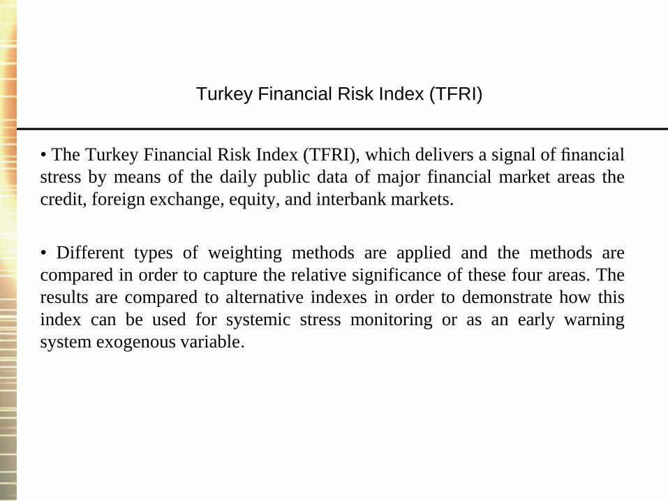
Turkey Financial Risk Index (TFRI)

• The Turkey Financial Risk Index (TFRI), which delivers a signal of financial

stress by means of the daily public data of major financial market areas the

credit, foreign exchange, equity, and interbank markets.

• Different types of weighting methods are applied and the methods are

compared in order to capture the relative significance of these four areas. The

results are compared to alternative indexes in order to demonstrate how this

index can be used for systemic stress monitoring or as an early warning

system exogenous variable.

Data & Methodology

• Four financial markets: interbank, credit, equity, and foreign exchange are

utilized to structure the index

• In order to provide continuous data market factors are selected according to

their availability. Continuous and reliable constructive data considerations

compensate index depth restrictions due to unavailable and missing data.

• The data set consists of daily values starting from 1 January 2004 until 24

January 2014

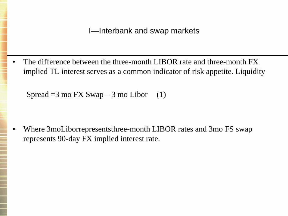
I—Interbank and swap markets

• The difference between the three-month LIBOR rate and three-month FX

implied TL interest serves as a common indicator of risk appetite. Liquidity

Spread =3 mo FX Swap – 3 mo Libor (1)

• Where 3moLiborrepresentsthree-month LIBOR rates and 3mo FS swap

represents 90-day FX implied interest rate.

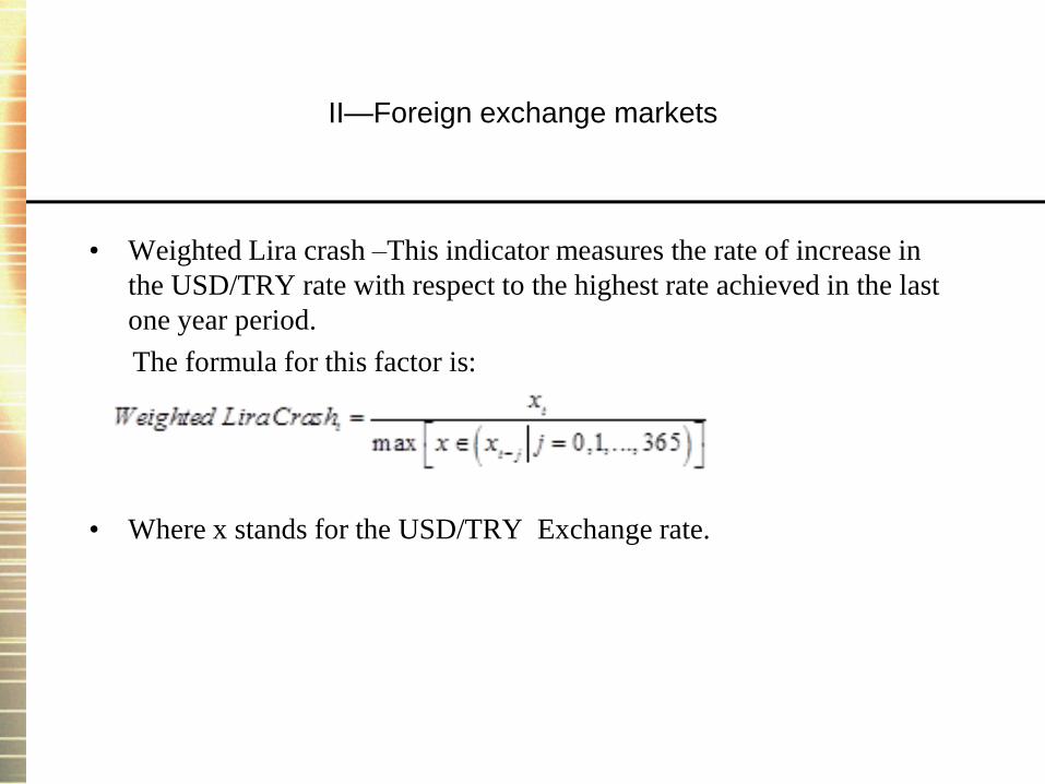
II—Foreign exchange markets

• Weighted Lira crash –This indicator measures the rate of increase in

the USD/TRY rate with respect to the highest rate achieved in the last

one year period.

The formula for this factor is:

• Where x stands for the USD/TRY Exchange rate.

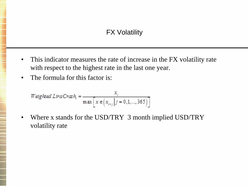
FX Volatility

• This indicator measures the rate of increase in the FX volatility rate

with respect to the highest rate in the last one year.

• The formula for this factor is:

• Where x stands for the USD/TRY 3 month implied USD/TRY

volatility rate

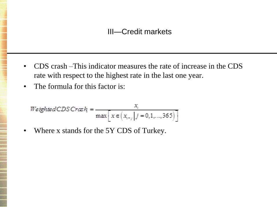
III—Credit markets

• CDS crash –This indicator measures the rate of increase in the CDS

rate with respect to the highest rate in the last one year.

• The formula for this factor is:

• Where x stands for the 5Y CDS of Turkey.

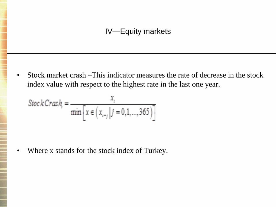
IV—Equity markets

• Stock market crash –This indicator measures the rate of decrease in the stock

index value with respect to the highest rate in the last one year.

• Where x stands for the stock index of Turkey.

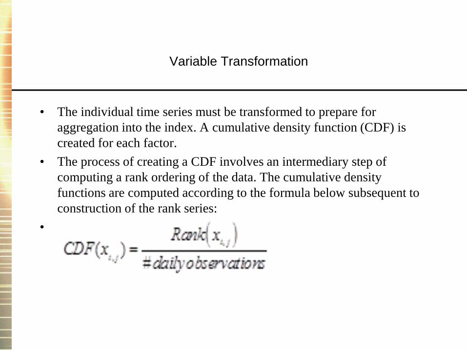
Variable Transformation

• The individual time series must be transformed to prepare for

aggregation into the index. A cumulative density function (CDF) is

created for each factor.

• The process of creating a CDF involves an intermediary step of

computing a rank ordering of the data. The cumulative density

functions are computed according to the formula below subsequent to

construction of the rank series:

•

Variable Weighting

• Once the CDF’s are calculated the contribution of each factor to the overall index has to

be determined according a weighting scheme. There are different ways of weighting in

the literature; this study has compared two alternative weighting schemes:

• (i) Equal weights – In this methodology equal importance is given to all factors

according to the common weighting scheme. The apparent problem is this methodology

is arbitrary and has no economic explanation to give all factors same weight.

• (ii) Principal component – Orthogonal eigenvectors of the variance–covariance matrix

of the data is a common approach for detection of the interaction among factors. Every

eigenvector reveals a certain proportion of the variability in the data. Mainly a single

factor is responsible for the greater part of the overall variability. An examination of the

variance–covariance matrix of the 5 series in this study reveals that there is more than a

single eigenvector specifically four eigenvectors, which together add up for about 95

percent of variability. Ultimately the weighting vector is shaped by taking the weighted

sum of the stated four eigenvectors. This methodology is not justified by any a priori

analysis which is one of the main drawbacks; consequently, the quality of results is

related to the features of the data.

Descriptive statistics

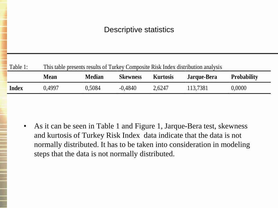
• As it can be seen in Table 1 and Figure 1, Jarque-Bera test, skewness

and kurtosis of Turkey Risk Index data indicate that the data is not

normally distributed. It has to be taken into consideration in modeling

steps that the data is not normally distributed.

Table 1: This table presents results of Turkey Composite Risk Index distribution analysis

Mean Median Skewness Kurtosis Jarque-Bera Probability

Index 0,4997 0,5084 -0,4840 2,6247 113,7381 0,0000

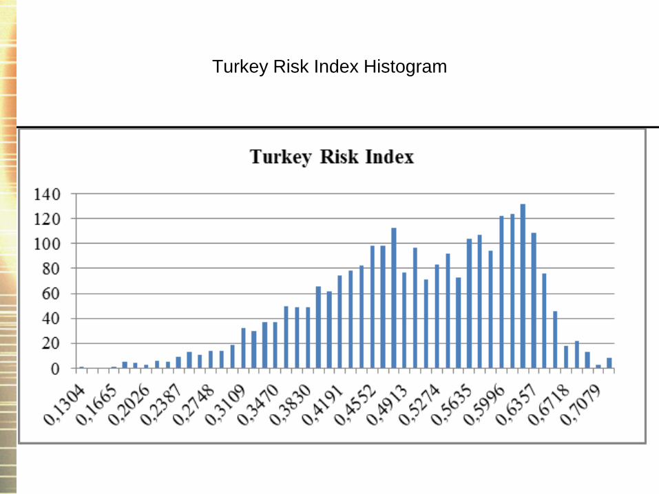
Turkey Risk Index Histogram

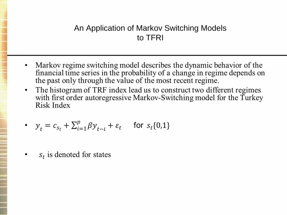
An Application of Markov Switching Models

to TFRI

Results

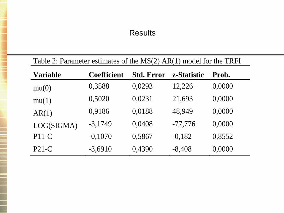
Table 2: Parameter estimates of the MS(2) AR(1) model for the TRFI

Variable Coefficient Std. Error z-Statistic Prob.

mu(0) 0,3588 0,0293 12,226 0,0000

mu(1) 0,5020 0,0231 21,693 0,0000

AR(1) 0,9186 0,0188 48,949 0,0000

LOG(SIGMA) -3,1749 0,0408 -77,776 0,0000

P11-C -0,1070 0,5867 -0,182 0,8552

P21-C -3,6910 0,4390 -8,408 0,0000

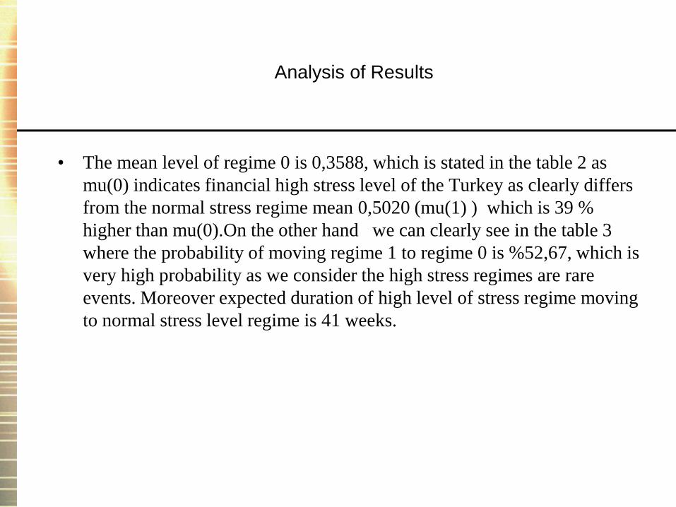
Analysis of Results

• The mean level of regime 0 is 0,3588, which is stated in the table 2 as

mu(0) indicates financial high stress level of the Turkey as clearly differs

from the normal stress regime mean 0,5020 (mu(1) ) which is 39 %

higher than mu(0).On the other hand we can clearly see in the table 3

where the probability of moving regime 1 to regime 0 is %52,67, which is

very high probability as we consider the high stress regimes are rare

events. Moreover expected duration of high level of stress regime moving

to normal stress level regime is 41 weeks.

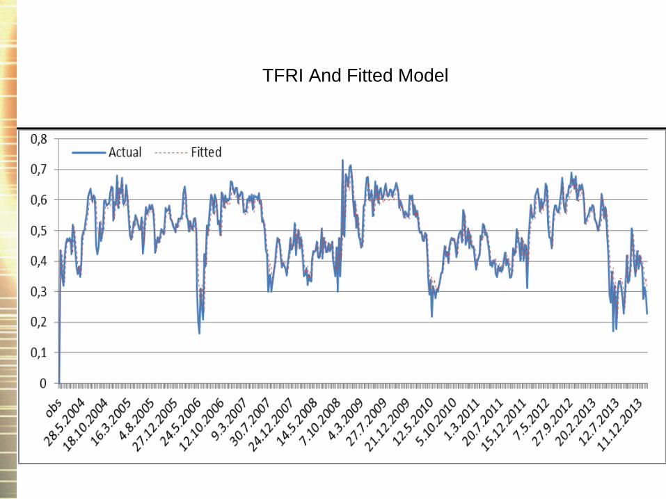
TFRI And Fitted Model

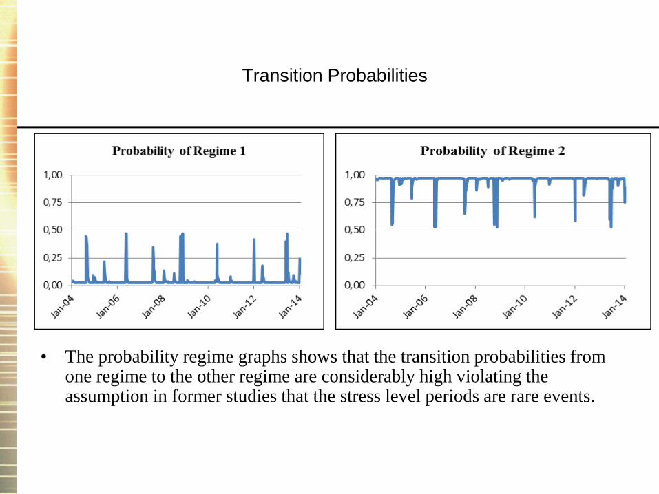
Transition Probabilities

• The probability regime graphs shows that the transition probabilities from one regime to the other regime are considerably high violating the assumption in former studies that the stress level periods are rare events.

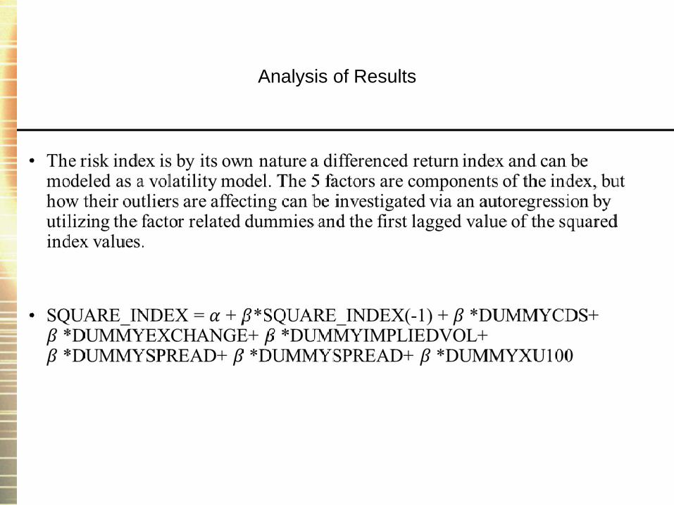
Garch Model

• The five factors are modeled separately by GARCH and the residuals

are calculated accordingly. The outlier residuals above two standard

deviations are flagged as one and the remainders are set to zero which

provides 5 new dummy variable endogenous time series as factors for

modeling the risk index.

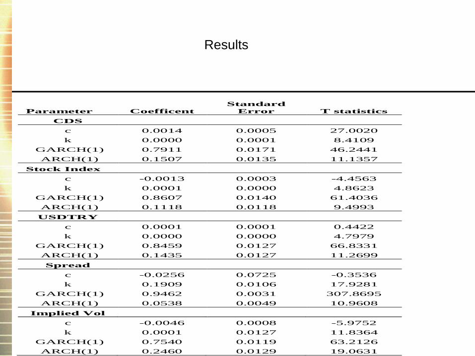
Results

Parameter Coefficent

Standard

Error T statistics

CDS

c 0.0014 0.0005 27.0020

k 0.0000 0.0001 8.4109

GARCH(1) 0.7911 0.0171 46.2441

ARCH(1) 0.1507 0.0135 11.1357

Stock Index

c -0.0013 0.0003 -4.4563

k 0.0001 0.0000 4.8623

GARCH(1) 0.8607 0.0140 61.4036

ARCH(1) 0.1118 0.0118 9.4993

USDTRY

c 0.0001 0.0001 0.4422

k 0.0000 0.0000 4.7979

GARCH(1) 0.8459 0.0127 66.8331

ARCH(1) 0.1435 0.0127 11.2699

Spread

c -0.0256 0.0725 -0.3536

k 0.1909 0.0106 17.9281

GARCH(1) 0.9462 0.0031 307.8695

ARCH(1) 0.0538 0.0049 10.9608

Implied Vol

c -0.0046 0.0008 -5.9752

k 0.0001 0.0127 11.8364

GARCH(1) 0.7540 0.0119 63.2126

ARCH(1) 0.2460 0.0129 19.0631

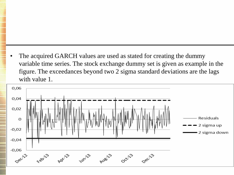
• The acquired GARCH values are used as stated for creating the dummy

variable time series. The stock exchange dummy set is given as example in the

figure. The exceedances beyond two 2 sigma standard deviations are the lags

with value 1.

Analysis of Results

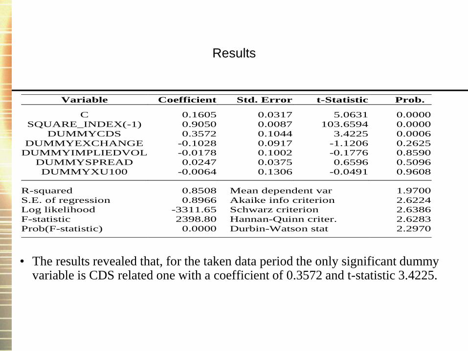
Results

• The results revealed that, for the taken data period the only significant dummy variable is CDS related one with a coefficient of 0.3572 and t-statistic 3.4225.

Variable Coefficient Std. Error t-Statistic Prob.

C 0.1605 0.0317 5.0631 0.0000

SQUARE_INDEX(-1) 0.9050 0.0087 103.6594 0.0000

DUMMYCDS 0.3572 0.1044 3.4225 0.0006

DUMMYEXCHANGE -0.1028 0.0917 -1.1206 0.2625

DUMMYIMPLIEDVOL -0.0178 0.1002 -0.1776 0.8590

DUMMYSPREAD 0.0247 0.0375 0.6596 0.5096

DUMMYXU100 -0.0064 0.1306 -0.0491 0.9608

R-squared 0.8508 Mean dependent var 1.9700

S.E. of regression 0.8966 Akaike info criterion 2.6224

Log likelihood -3311.65 Schwarz criterion 2.6386

F-statistic 2398.80 Hannan-Quinn criter. 2.6283

Prob(F-statistic) 0.0000 Durbin-Watson stat 2.2970

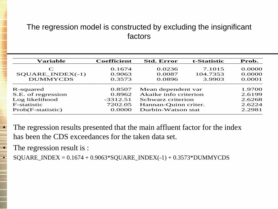
The regression model is constructed by excluding the insignificant

factors

• The regression results presented that the main affluent factor for the index

has been the CDS exceedances for the taken data set.

• The regression result is :

• SQUARE_INDEX = 0.1674 + 0.9063*SQUARE_INDEX(-1) + 0.3573*DUMMYCDS

Variable Coefficient Std. Error t-Statistic Prob.

C 0.1674 0.0236 7.1015 0.0000

SQUARE_INDEX(-1) 0.9063 0.0087 104.7353 0.0000

DUMMYCDS 0.3573 0.0896 3.9903 0.0001

R-squared 0.8507 Mean dependent var 1.9700

S.E. of regression 0.8962 Akaike info criterion 2.6199

Log likelihood -3312.51 Schwarz criterion 2.6268

F-statistic 7202.05 Hannan-Quinn criter. 2.6224

Prob(F-statistic) 0.0000 Durbin-Watson stat 2.2981

Conclusion

• A new composite index is proposed by combining different parameters like FX Implied Volatilities, CDS and Interest Rates levels. This new risk index that is modeled by GARCH and Markov autoregressive based models for forecasting and identifying thresholds to be better and efficient in comparison to single indicators

• As it can be seen many indicators can be used for estimating market tension levels and a common composite index could be used as a general indicator for market players. Eventually this index can be modeled by using appropriate econometric forecasting procedures. The established index can also be used as an exogenous input for modeling other variables in the market.